Irina Ginzburg and Dominique d’Humières -...
46
www.cemagref.fr Irina Ginzburg and Dominique d’Humières Cemagref, Antony, France, Water and Environmental Engineering École Normale Supérieure, Paris, France Laboratory of Statistical Physics Some elements of Lattice Boltzmann method for hydrodynamic and anisotropic advection-diffusion problems Paris, 20 December, 2006 Slide 1
Transcript of Irina Ginzburg and Dominique d’Humières -...
www.cemagref.fr
Irina Ginzburg and Dominique d’Humières
Cemagref, Antony, France,Water and Environmental Engineering
École Normale Supérieure, Paris, FranceLaboratory of Statistical Physics
Some elements of Lattice Boltzmann methodfor hydrodynamicand anisotropic advection-diffusion problems
Paris, 20 December, 2006
Slide 1

– U. Frisch, D. d’Humières, B. Hasslacher, P. Lallemand,Y. Pomeau, and J.P. Rivet, Lattice gas hydrodynamics in twoand three dimensions., Complex Sys., 1, 1987
– F. J. Higuera and J. Jiménez, Boltzmann approach to latticegas simulations. Europhys. Lett., 9, 1989
– D. d’Humières, Generalized Lattice-Boltzmann Equations,AIAA Rarefied Gas Dynamics: Theory and Simulations, 59,1992
– D. d’Humières, I. Ginzburg, M. Krafczyk, P. Lallemand andL.-S. Luo, Multiple-relaxation-time lattice Boltzmann modelsin three dimensions, Phil. Trans. R. Soc. Lond. A 360, 2005
– I. Ginzburg, Equilibrium-type and Link-type LatticeBoltzmann models for generic advection andanisotropic-dispersion equation, Adv Water Resour, 28, 2005
Slide 2
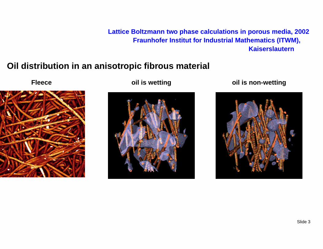
Lattice Boltzmann two phase calculations in porous media, 2002Fraunhofer Institut for Industrial Mathematics (ITWM),
Kaiserslautern
Oil distribution in an anisotropic fibrous material
oil is wetting oil is non-wettingFleece
Slide 3
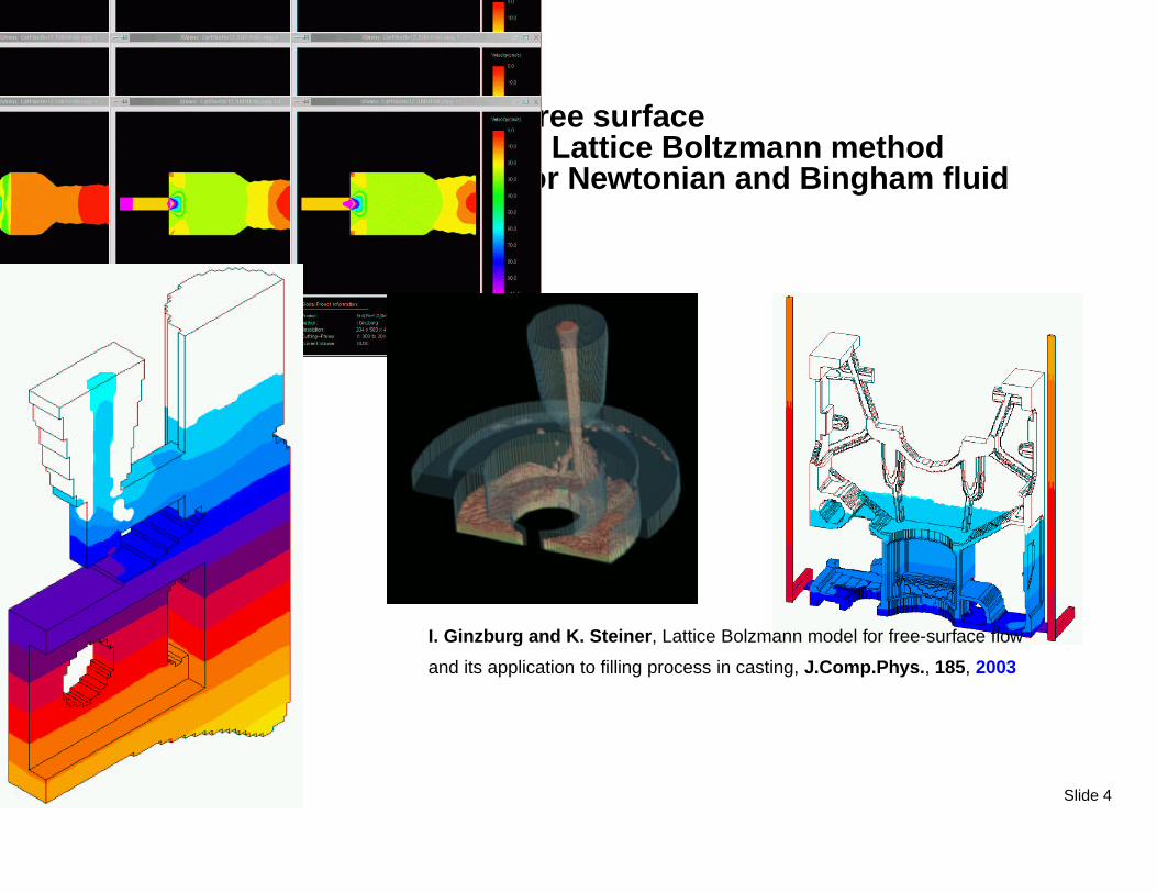
Free surfaceLattice Boltzmann method
for Newtonian and Bingham fluid
I. Ginzburg and K. Steiner, Lattice Bolzmann model for free-surface flow
and its application to filling process in casting, J.Comp.Phys., 185, 2003
Slide 4
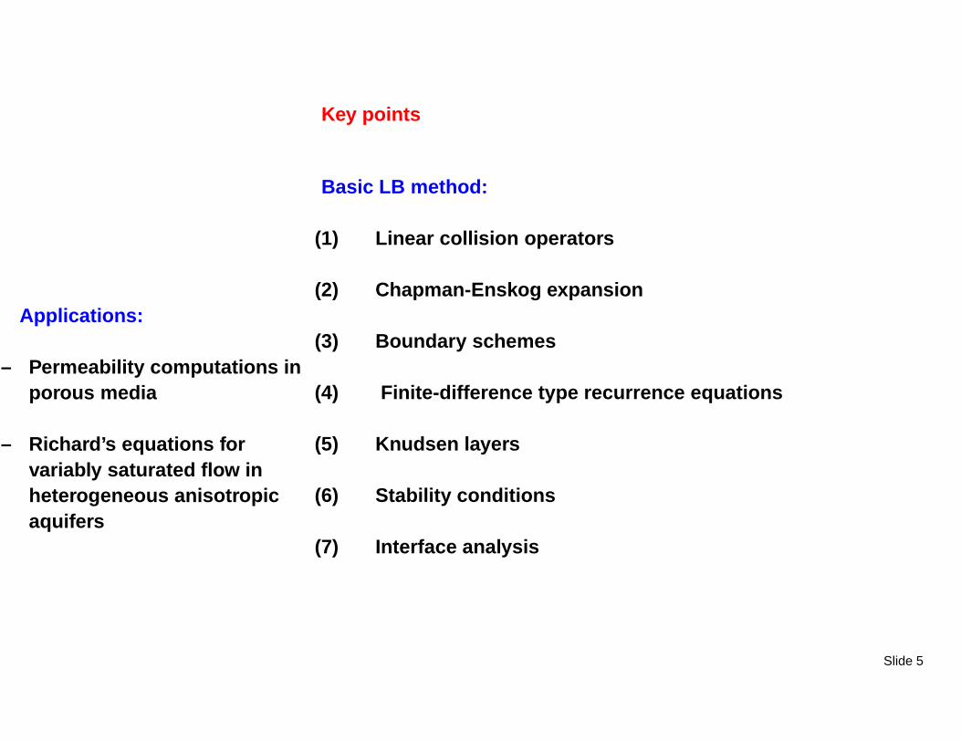
Key points
Basic LB method:
(1) Linear collision operators
(2) Chapman-Enskog expansion
(3) Boundary schemes
(4) Finite-difference type recurrence equations
(5) Knudsen layers
(6) Stability conditions
(7) Interface analysis
Applications:
– Permeability computations inporous media
– Richard’s equations forvariably saturated flow inheterogeneous anisotropicaquifers
Slide 5
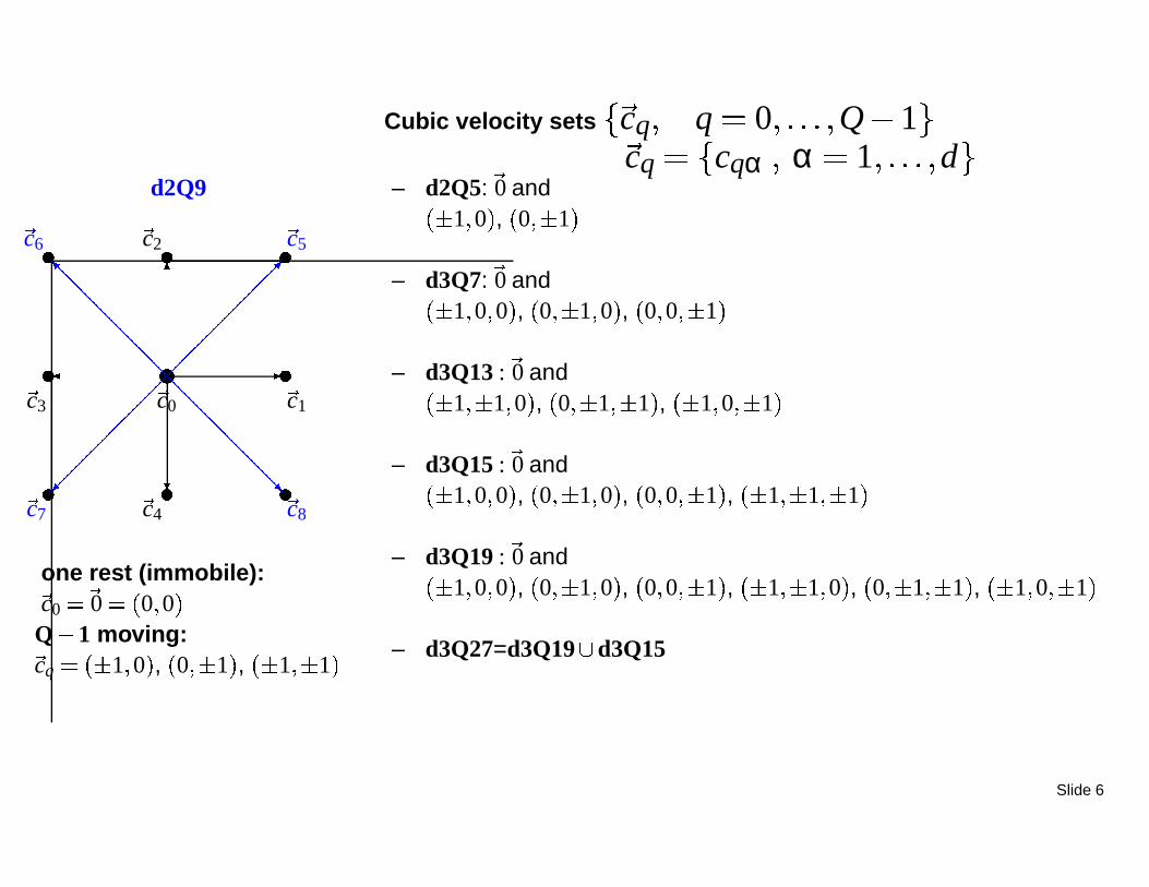
Cubic velocity sets cq q 0 Q 1 cq cqα α 1 d
d2Q9
c0
c1
c2
c4
c3
c5
c6
c7
c8
one rest (immobile):c0
0 0 0
Q 1 moving:cq 1 0 , 0 1 , 1 1
– d2Q5:
0 and
1 0 , 0 1
– d3Q7:
0 and
1 0 0 , 0 1 0 , 0 0 1
– d3Q13 :
0 and
1 1 0 , 0 1 1 , 1 0 1
– d3Q15 :
0 and
1 0 0 , 0 1 0 , 0 0 1 , 1 1 1
– d3Q19 :
0 and
1 0 0 , 0 1 0 , 0 0 1 , 1 1 0 , 0 1 1 , 1 0 1
– d3Q27=d3Q19 d3Q15
Slide 6
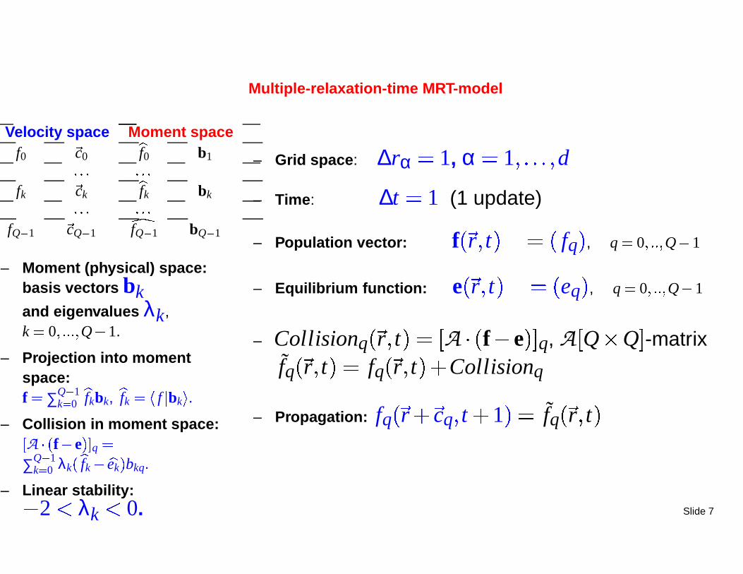
Multiple-relaxation-time MRT-model
Velocity space Moment spacef0
c0
f0 b1
fk
ck
fk bk
fQ 1
cQ 1
fQ 1 bQ 1
– Moment (physical) space:basis vectors bkand eigenvalues λk,k 0 Q 1.
– Projection into momentspace:f ∑Q 1
k 0
fkbk,
fk f bk .– Collision in moment space:
A f e q
∑Q 1k 0 λk
fk
ek bkq.
– Linear stability: 2 λk 0.
– Grid space: ∆rα 1, α 1 d
– Time: ∆t 1 (1 update)
– Population vector: f r t fq , q 0 Q 1
– Equilibrium function: e r t eq , q 0 Q 1
– Collisionq r t A f e q, A Q Q -matrixfq r t fq r t Collisionq
– Propagation: fq r cq t 1 fq r t
Slide 7

MRT basis of d2Q9 modeld2Q9 : bk k 1 9
b1 q 1
b2 q cqx
b3 q cqy
b4 q 3c2q
4 c2q c2
qx c2qy
b5 q 2c2qx
c2q
b6 q cqxcqy
b7 q cqx 3c2q
5
b8 q cqy 3c2q
5
b9 q 12 9c4
q
21c2q 8
b1 b2 b3 b4 b5 b6 b7 b8 b9
1 0 0 4 0 0 0 0 41 1 0 1 1 0 2 0 21 1 1 2 0 1 1 1 11 0 1 1 1 0 0 2 21 1 1 2 0 1 1 1 11 1 0 1 1 0 2 0 21 1 1 2 0 1 1 1 11 0 1 1 1 0 0 2 21 1 1 2 0 1 1 1 1
Eigenvaluesλ 0 λ 1 λ 2 λ 1 λ 2 λ 3 λ 3 λ 4 λ 4
λ
0 0, λ 1 0, λ 2 0,
λ
1 νξ, λ 2 ν, λ
3 ν.
Slide 8

Link-model LM, (2005)
c1
c2
c4
c3
c5
c6
c7
c8
f0f1
f2
f2
f1
f5f6
f5 f6
– Decomposition:
fq f
q f
q
– Symmetric part:
f
q 12 fq fq
– Antisymmetric
part: f
q 12 fq fq
– Link: cq cq , cq cq
– Collisionq=pq mq
– Symmetric collision part: pq λ
q f
q
e
q
– Antisymmetric collision part: mq λ q f
q
e
q
– Local equilibrium: eq e
q e
q , eq eq f
Slide 9

Microscopic conservation laws with Link Model
– Conserved mass quantity ρ r t :
Let ρ r t ∑Q 1q 0 fq ∑Q 1
q 0 f
q
∑Q 1q 0 eq ∑Q 1
q 0 e
q , then
∑Q 1q 0 λ
q f
q
e
q 0 if λ
q λ .
– Conserved d dimensional momentum quantity
j r t :
Let
j r t ∑Q 1q 1 fq
cq ∑Q 1q 1 f
q
cq
∑Q 1q 1 eq
cq ∑Q 1q 1 e
q
cq, then
∑Q 1q 1 λ q f
q
e
q cq 0 if λ q λ .
– Mass+momentum with LM:two-relaxation-time operator,TRT only !!!
– BGK: λ λ λ(Qian, d’Humières &
Lallemand, 1992)
A f e q λ fq eq
BGK TRT MRT
BGK TRT LM
Slide 10

Following idea of Chapman-Enskog (1916-1917)
– Let ε 1L
with L as a characteristiclength
– Let x εx
– Let t1 εt, t2 ε2t,
∂t ε∂t1 ε2∂t2
– Population expansion around the equilibrium:
fq eq ε f 1
q ε2 f 2
q
– Collision components :
p n
q A f n
q ,
m n
q A f n
q .
– Macroscopic laws:
∑Q 1q 0 p 1
q p 2
q 0,
∑Q 1q 0 m 1
q m 2
q cq 0.
Slide 11
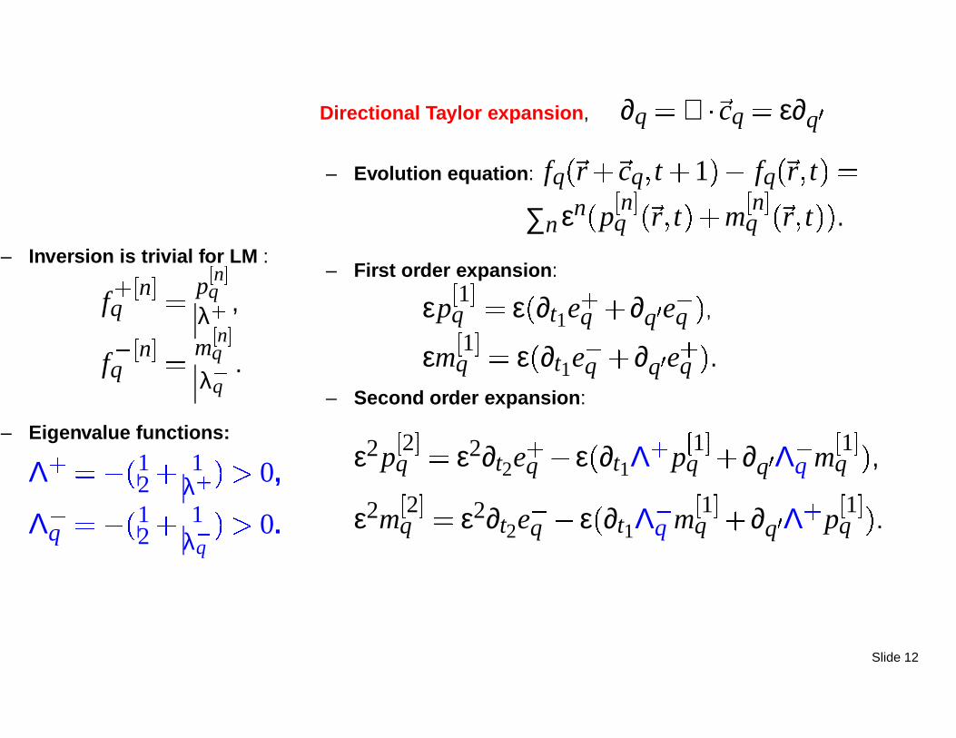
Directional Taylor expansion, ∂q ∇ cq ε∂q
– Inversion is trivial for LM :
f n
q p n
qλ ,
f
n
q m n
q
λ q.
– Eigenvalue functions:
Λ 12 1
λ 0,
Λ
q 12 1
λ q
0.
– Evolution equation: fq r cq t 1 fq r t
∑n εn p n
q r t m n
q r t .– First order expansion:
εp 1
q ε ∂t1e
q ∂q e
q ,
εm 1
q ε ∂t1e
q ∂q e
q .– Second order expansion:
ε2p 2
q ε2∂t2e q
ε ∂t1Λ p 1
q ∂q Λ
q m 1
q ,ε2m 2
q ε2∂t2e
q ε ∂t1Λ
q m 1
q ∂q Λ p 1
q .
Slide 12
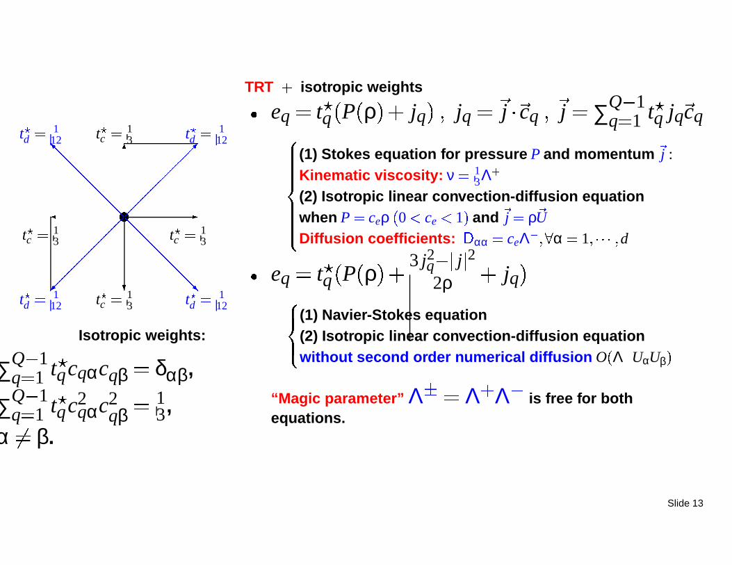
TRT isotropic weights
t c 13
t c 13
t c 13
t c 13
t d
112t d
112
t d
112 t d
112
Isotropic weights:
∑Q 1q 1 t
qcqαcqβ δαβ,
∑Q 1q 1 t
qc2qαc2
qβ
13,
α β.
eq t
q P ρ jq jq
j cq
j ∑Q 1q 1 t
q jq
cq
(1) Stokes equation for pressure P and momentum
j :Kinematic viscosity: ν 1
3Λ
(2) Isotropic linear convection-diffusion equationwhen P ceρ 0 ce 1 and
j ρ
U
Diffusion coefficients: αα ceΛ
α 1 d eq t
q P ρ 3 j2q j
2
2ρ jq
(1) Navier-Stokes equation(2) Isotropic linear convection-diffusion equationwithout second order numerical diffusion O Λ UαUβ
“Magic parameter” Λ Λ Λ
is free for bothequations.
Slide 13

Incompressible Navier-Stokes equation
Let P c2s ρ
Mach number:Ma U
cs,
U is characteristicvelocity.
Sound velocity:0 c2
s 1best : c2
s 13
(Lallemand & Luo, 2000)
– MRT TRT BGK with forcing S
q :
fq r cq t 1 fq r t pq mq S
q .
Incompressible limit, Ma 0:
ρ ρ0 1 Ma2P P P ρ P ρ0
ρ0U2 ,
∇ u O Ma2∂tP O ε3 if U O ε
ρ0∂tu ρ0∇ u
u
∇P ∇ ρ0ν∇ u
F O ε3 O Ma2
Force:
F ∑Q 1q 1 S
q
cq
j ∑Q 1q 1 fq
cq 12
F , u
jρ0
Slide 14
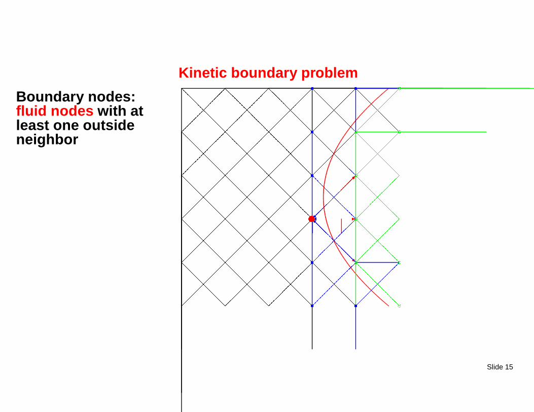
Kinetic boundary problem
Boundary nodes:fluid nodes with atleast one outsideneighbor
Slide 15

Dirichlet velocity conditionvia the bounce-back
fq rb fq rb 2e
q rb δqcq
Dirichlet pressure conditionvia the anti-bounce-back
fq rb fq rb
2e
q rb δq
cq
h
B∆=0.5 ?
Bounce-back:H = h + 2 ∆
Η − ?
effective channel width H -
B
Boundary conditions
No slip
B
Free slip SpecularReflection
Bounce-back
Periodic
Slide 16

No-slip condition via bounce-back reflectionI. Ginzburg & P. M. Adler, J.Phys.II France, 1994
Cqδq
Cqδq
fq
fq
h H ?
H h if Λ 316
H h if Λ 316
H h if Λ
316
H ∞ if Λ Λ
and ν ∞ (BGK)
– First order closure relation:
jq rb 12∂q jq rb O ε2 , δq 1
2
– Second order closure relation:
jq rb 12∂q jq rb 1
243Λ ∂2
q jq rb O ε3
– For Poiseuille flow, effective width H of the channel is
H2 h2 163 Λ 1
Slide 17

Permeability measurements with the bounce-back reflection
k Λ
k Λ 12
k Λ 12
, ν 13Λ
– Darcy law:
ν
j K
F ∇P
– Permeability is viscositydependent for BGK,
Λ 9ν2
– Permeability is absolutelyviscosity independent forTRT
if Λ Λ Λ
and Λ is fixed
– WHY ??
Λ 203, φ 0 965 903, φ 0 941TRT BGK TRT BGK
1 8 10 13 0 077 10 13 0 08315 2 2 8 10 12 4 699 10 13 2 236
Slide 18
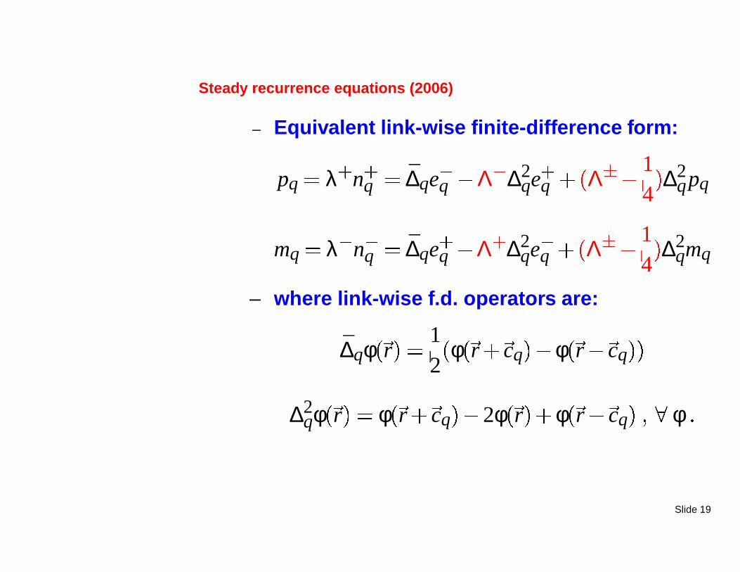
Steady recurrence equations (2006)
– Equivalent link-wise finite-difference form:
pq λ n
q ∆qe
q
Λ ∆2qe
q Λ 14 ∆2
qpq
mq λ n
q ∆qe
q
Λ ∆2qe
q Λ 14 ∆2
qmq
– where link-wise f.d. operators are:
∆qφ r 12 φ r cq φ r cq
∆2qφ r φ r cq 2φ r φ r cq φ
Slide 19
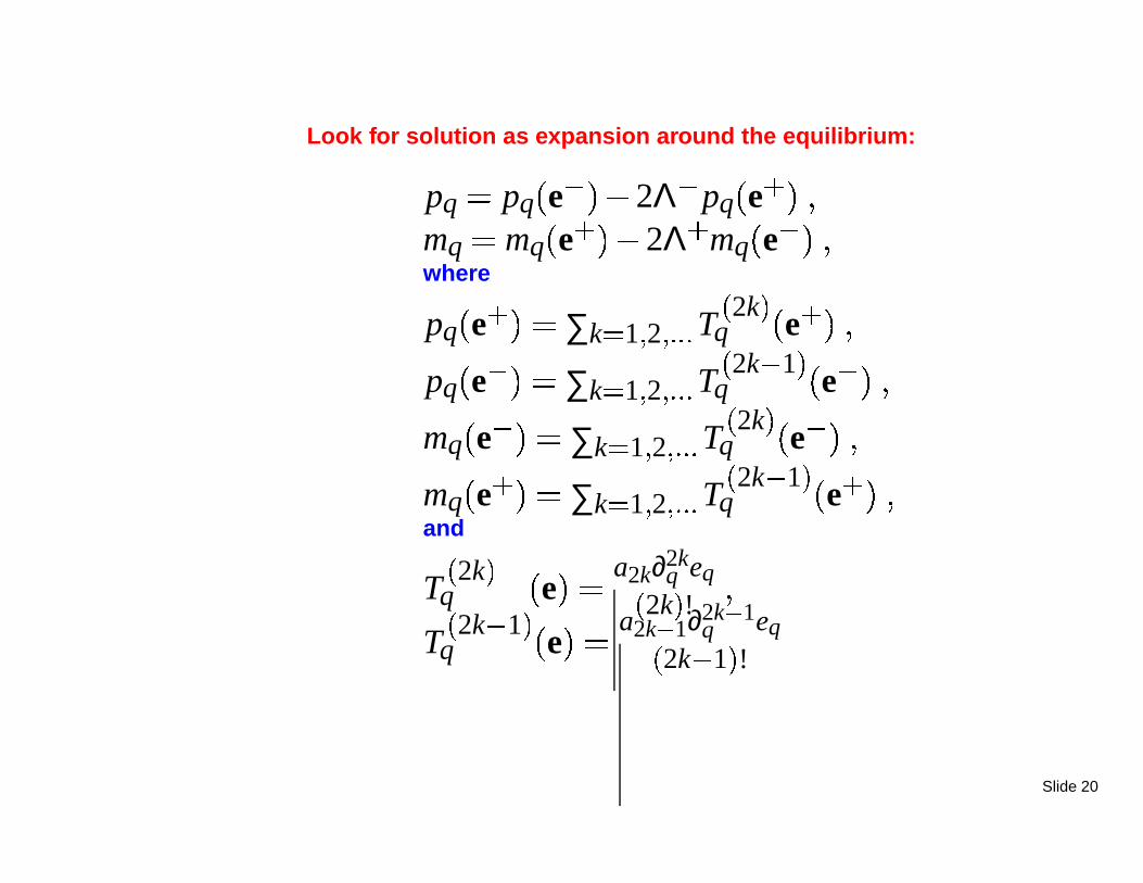
Look for solution as expansion around the equilibrium:
pq pq e 2Λ
pq e
mq mq e 2Λ mq e
where
pq e ∑k 1
2
T 2k
q e
pq e ∑k 1
2
T 2k 1
q e
mq e ∑k 1
2
T 2k
q e
mq e ∑k 1
2
T 2k 1
q e
and
T 2k
q e a2k∂2kq eq
2k !
T 2k 1
q e a2k 1∂2k 1q eq
2k 1 !
Slide 20

Solution for the coefficients of the series, k 1:
a2k 1 1
2 Λ 14 ∑1 n k a2n 1
2k 1 !
2n 1 ! 2 k n !
a2k 1 2 Λ 14 ∑1 n k a2n
2k !
2n ! 2 k n !
– Non-dimensional steady solutions on the fixed grid
j
jρ0U P P P0
ρ0U2 are the same if
Ma Ucs
, Fr U2
gL , Re ULν and Λ are fixed
– Provided that this property is shared by the microscopicboundary schemes,
the permeability is the same if Λ is fixed !!!
Slide 21
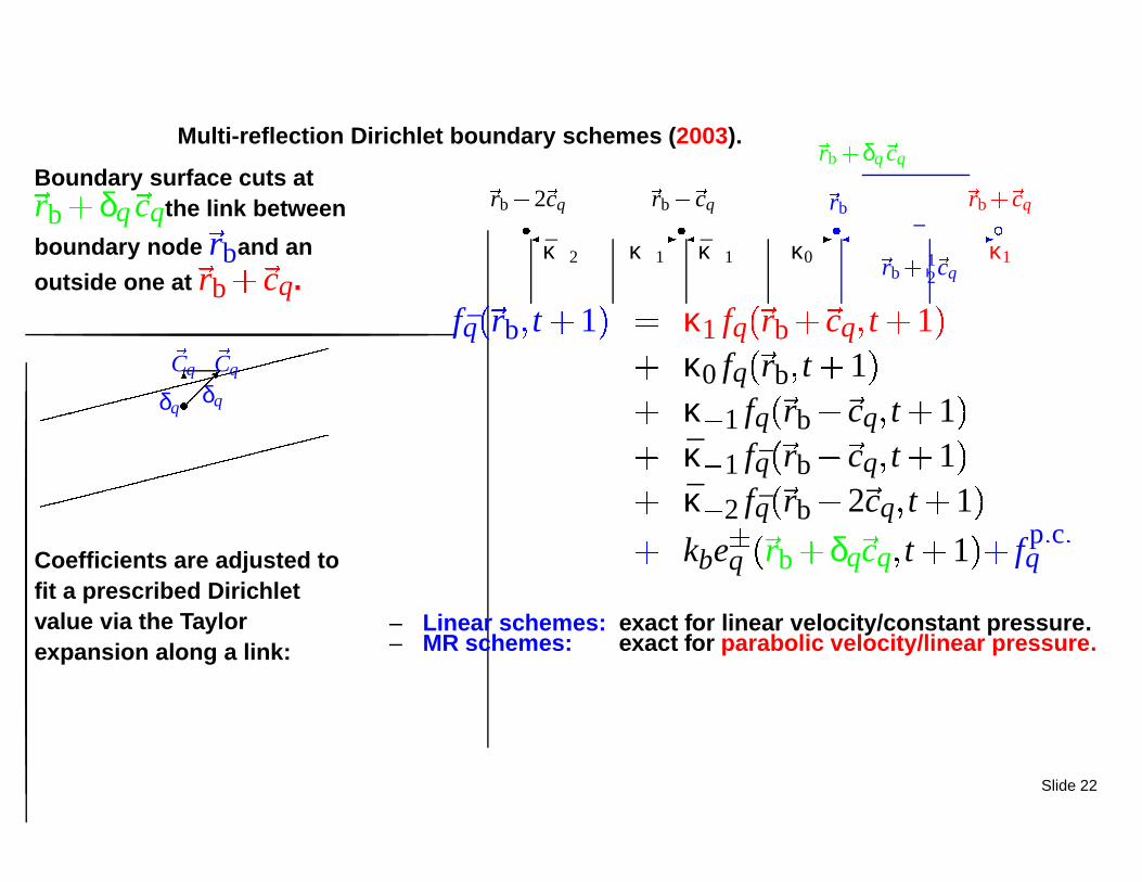
Multi-reflection Dirichlet boundary schemes (2003).
Boundary surface cuts atrb δq
cqthe link between
boundary node
rband an
outside one at
rb cq.
Cq
δq
Cq
δq
Coefficients are adjusted tofit a prescribed Dirichletvalue via the Taylorexpansion along a link:
rb 2 cq
rb cq
rb
rb cq
κ1rb
12
cq
rb δq
cq
κ 2
κ 1
κ 1
κ0
fq rb t 1 κ1 fq rb cq t 1
κ0 fq rb t 1
κ 1 fq rb cq t 1
κ 1 fq rb cq t 1
κ 2 fq rb 2 cq t 1
kbe
q rb δq
cq t 1 f p c
q
– Linear schemes: exact for linear velocity/constant pressure.– MR schemes: exact for parabolic velocity/linear pressure.
Slide 22
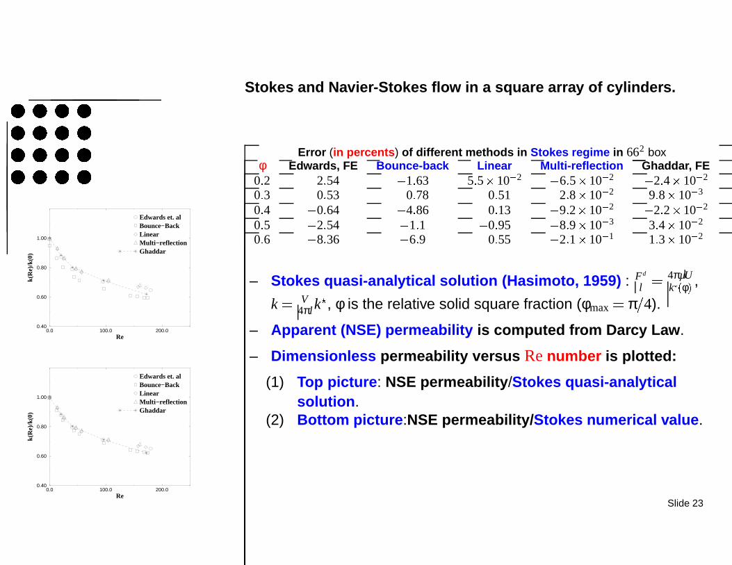
Stokes and Navier-Stokes flow in a square array of cylinders.
0.0 100.0 200.0Re
0.40
0.60
0.80
1.00
k(R
e)/k
(0)
Edwards et. alBounce−BackLinearMulti−reflectionGhaddar
0.0 100.0 200.0Re
0.40
0.60
0.80
1.00
k(R
e)/k
(0)
Edwards et. alBounce−BackLinearMulti−reflectionGhaddar
Error (in percents) of different methods in Stokes regime in 662 boxφ Edwards, FE Bounce-back Linear Multi-reflection Ghaddar, FE
0 2 2 54 1 63 5 5 10 2 6 5 10 2 2 4 10 2
0 3 0 53 0 78 0 51 2 8 10 2 9 8 10 3
0 4 0 64 4 86 0 13 9 2 10 2 2 2 10 2
0 5 2 54 1 1 0 95 8 9 10 3 3 4 10 2
0 6 8 36 6 9 0 55 2 1 10 1 1 3 10 2
– Stokes quasi-analytical solution (Hasimoto, 1959) : Fd
l
4πµUk φ ,
k V4πlk
, φ is the relative solid square fraction (φmax π 4).
– Apparent (NSE) permeability is computed from Darcy Law.
– Dimensionless permeability versus Re number is plotted:
(1) Top picture: NSE permeability/Stokes quasi-analyticalsolution.
(2) Bottom picture:NSE permeability/Stokes numerical value.
Slide 23

Application of multi-reflections for moving boundaries
Pressure distribution around three spheres moving in a circular tube
Slide 24

Solutions beyond the Chapman-Enskog expansion
-1
-0.8
-0.6
-0.4
-0.2
0
0.2
0.4
0.6
0.8
0 1 2 3 4 5 6 7 8
Nor
mal
ized
Knu
dsen
laye
r
y, [l.u]
Symmetric part, L=8
-1
-0.8
-0.6
-0.4
-0.2
0
0.2
0.4
0.6
0.8
0 2 4 6 8 10 12 14 16 18
Nor
mal
ized
Knu
dsen
laye
r
y, [l.u]
Symmetric part, L=17
Λ 14: accommodation
oscillates, (Λ 3256, Λ 3
16)
Λ 14: it decreases
exponentially (Λ 32)
pq pchq g
q , mq mchq g
q
g
q Λ 14 ∆2
qg
q ∑Q 1q 0 g
q 0
g
q Λ 14 ∆2
qg
q ∑Q 1q 1 g
q
cq 0
Example of Knudsen layer in horizontal channel:e.g.,exact Poiseuille flow using non-linear equilibrium
g q 3c2
qx
1 t
qK y c2qy
g
q 3c2qx
1 t
qK
y cqy
K y k 1 ry
0 k
2 r
y0 , r0 2 Λ 1
2 Λ 1r0 and 1 r0 obey: r 1 2 4Λ r 1 2
Λ 14: accommodation in boundary node
Slide 25
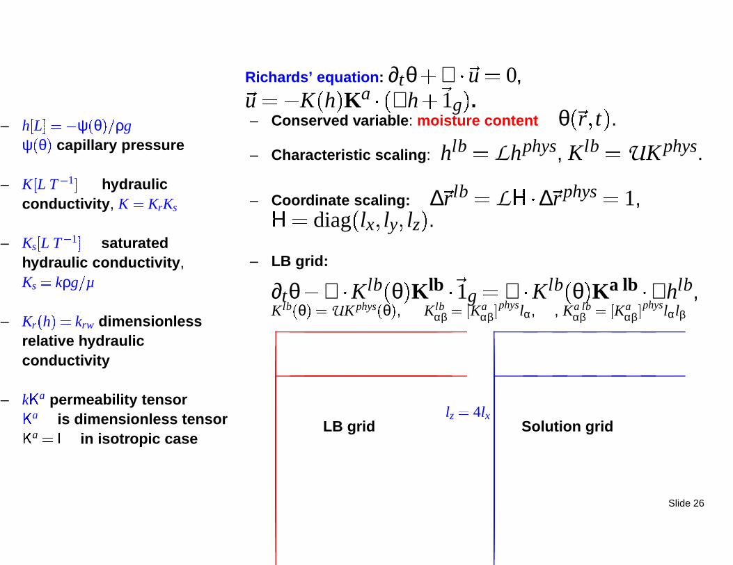
Richards’ equation: ∂tθ ∇ u 0,u K h Ka ∇h
1g .– h L ψ θ ρg
ψ θ capillary pressure
– K L T 1 hydraulicconductivity, K KrKs
– Ks L T 1 saturatedhydraulic conductivity,Ks kρg µ
– Kr h krw dimensionlessrelative hydraulicconductivity
– k a permeability tensor
a is dimensionless tensor
a in isotropic case
– Conserved variable: moisture content θ r t .– Characteristic scaling: hlb Lhphys, Klb UK phys.
– Coordinate scaling: ∆ rlb L ∆ rphys 1,
diag lx ly lz .– LB grid:
∂tθ ∇ Klb θ Klb
1g ∇ Klb θ Ka lb ∇hlb,Klb θ UK phys θ , Klb
αβ Kaαβ physlα, , Ka lb
αβ Kaαβ physlαlβ
LB gridlz 4lx
Solution grid
Slide 26
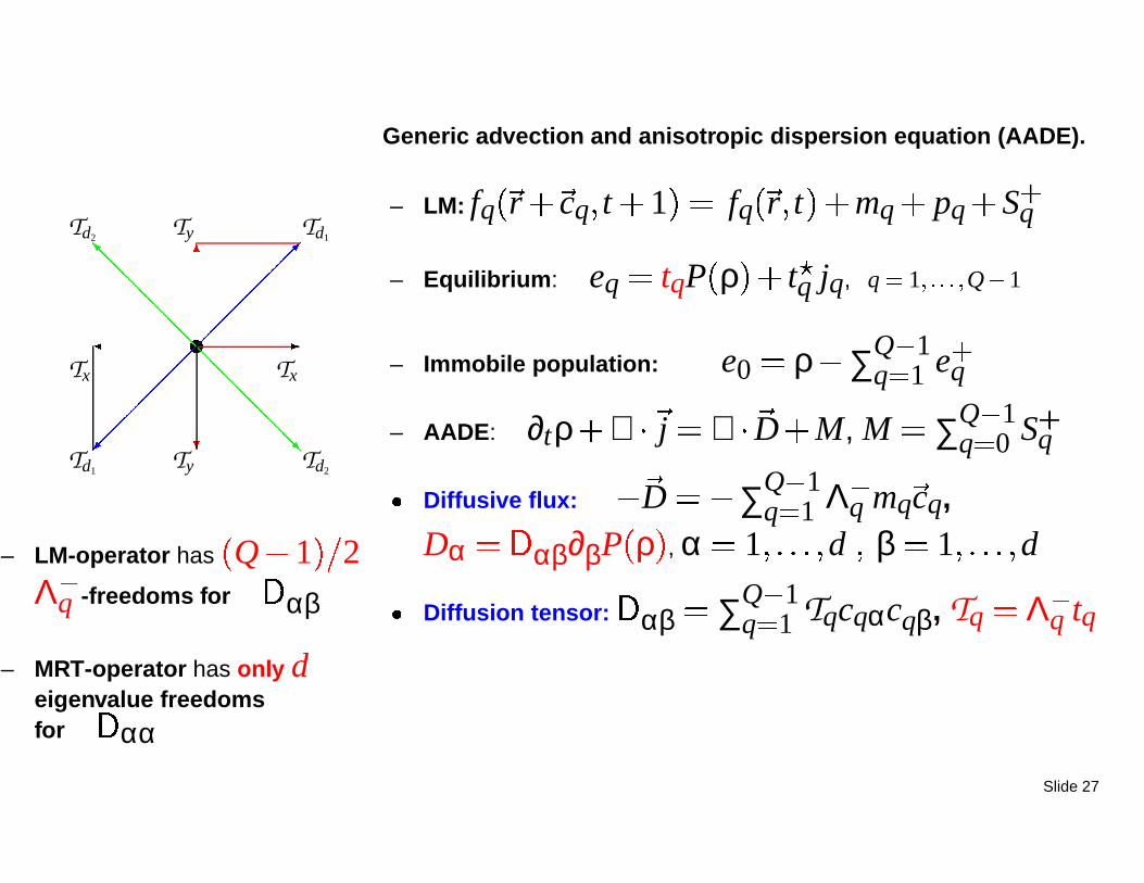
Generic advection and anisotropic dispersion equation (AADE).
Tx
Ty
Ty
Tx
Td1Td2
Td1Td2
– LM-operator has Q 1 2Λ
q -freedoms for αβ
– MRT-operator has only deigenvalue freedomsfor αα
– LM: fq r cq t 1 fq r t mq pq S
q
– Equilibrium: eq tqP ρ t
q jq, q 1 Q 1
– Immobile population: e0 ρ ∑Q 1q 1 e
q
– AADE: ∂tρ ∇
j ∇
D M, M ∑Q 1q 0 S
q
Diffusive flux:
D ∑Q 1q 1 Λ
q mq
cq,
Dα αβ∂βP ρ , α 1 d β 1 d
Diffusion tensor: αβ ∑Q 1q 1 Tqcqαcqβ, Tq Λ
q tq
Slide 27
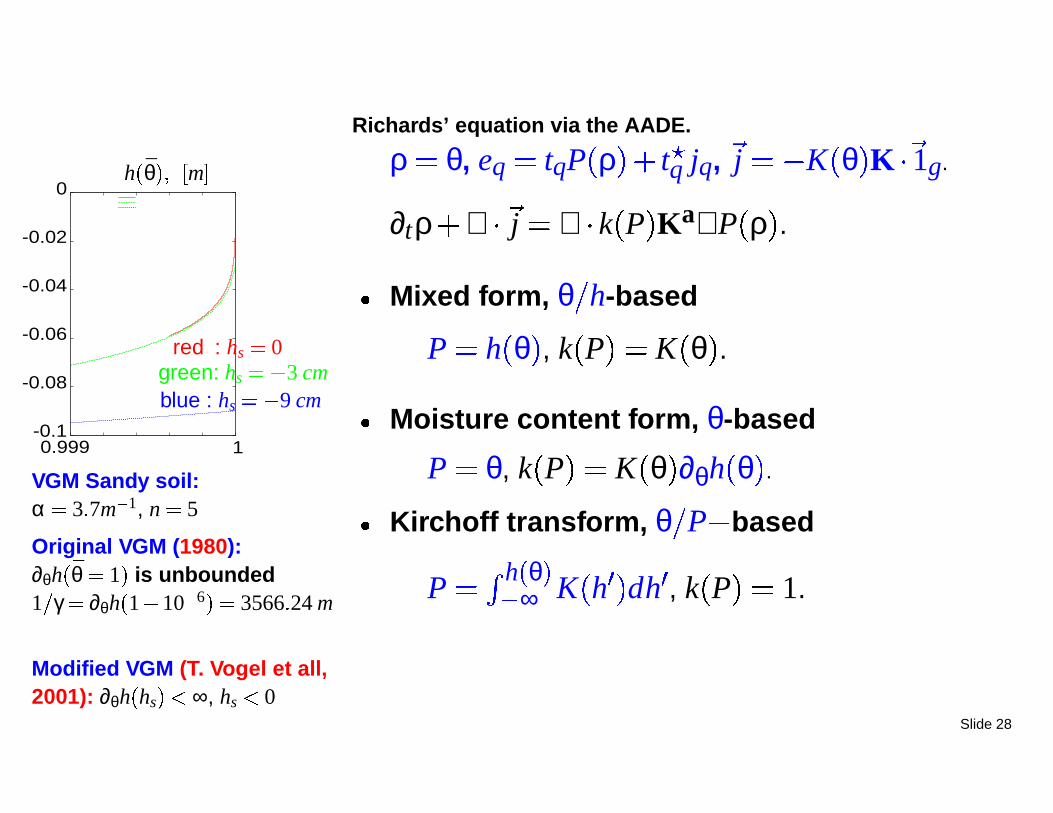
Richards’ equation via the AADE.
ρ θ, eq tqP ρ t
q jq,
j K θ K
1g.
∂tρ ∇
j ∇ k P Ka∇P ρ .
Mixed form, θ h-based
P h θ , k P K θ . Moisture content form, θ-based
P θ, k P K θ ∂θh θ .
Kirchoff transform, θ P based
P
h θ ∞ K h dh , k P 1.
h θ m
-0.1
-0.08
-0.06
-0.04
-0.02
0
0.999
1
red : hs 0green: hs 3 cmblue : hs 9 cm
VGM Sandy soil:α 3 7m 1, n 5
Original VGM (1980):∂θh θ 1 is unbounded1 γ ∂θh 1 10 6 3566 24 m
Modified VGM (T. Vogel et all,2001): ∂θh hs ∞, hs 0
Slide 28
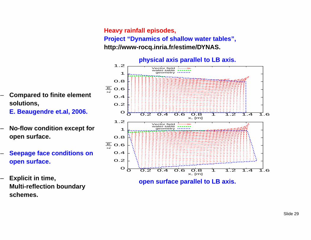
Heavy rainfall episodes,Project “Dynamics of shallow water tables”,http://www-rocq.inria.fr/estime/DYNAS.
physical axis parallel to LB axis.
0
0.2
0.4
0.6
0.8
1
1.2
0 0.2 0.4 0.6 0.8 1 1.2 1.4 1.6
z, [m]
x, [m]
Vector fieldwater-table
geometry
0
0.2
0.4
0.6
0.8
1
1.2
0 0.2 0.4 0.6 0.8 1 1.2 1.4 1.6
z, [m]
x, [m]
Vector fieldwater-table
geometry
open surface parallel to LB axis.
– Compared to finite elementsolutions,E. Beaugendre et.al, 2006.
– No-flow condition except foropen surface.
– Seepage face conditions onopen surface.
– Explicit in time,Multi-reflection boundaryschemes.
Slide 29

Reduced vertical velocity on open surface, uz Ks.
SAND on non-aligned grid
-0.2
-0.1
0
0.1
0.2
0.3
0.4
0.5
0.6
0 0.2 0.4 0.6 0.8 1 1.2 1.4
u_z/
Ks
x, [m]
hs=0, FE hs=-9cm, LB, Nodehs=-9cm, LB, Wall
YLC and SAND, on aligned grid
-0.2
-0.1
0
0.1
0.2
0.3
0.4
0.5
0.6
0 0.2 0.4 0.6 0.8 1 1.2 1.4
u_z/
Ks
x, [m]
YLC, hs=-2cm, FEYLC, hs=-2cm, LB
SAND, hs=0, FESAND, hs=0, LB
Relative ex-filtration fluxes
SCL on non-aligned grid
0
0.1
0.2
0.3
0.4
0.5
0 2 4 6 8 10 12 14 16 18
Rel
ativ
e E
xfilt
ratio
n
time, [h]
FE, hs=0 LB: hs=0, it=80LB, hs=0, it=20
YLC on aligned grid
0
0.1
0.2
0.3
0.4
0.5
0 1 2 3 4 5 6 7 8R
elat
ive
Exf
iltra
tion
time, [h]
FE, hs=-2cmLB, hs=-2cm
Compared to finite elementsolutions,E. Beaugendre et.al, 2006.
Rainfall intensity isqin 0 1Ks for all soils.
FE grid with 280 nodes onthe open surface.
LB grid with 70 nodes on theopen surface.
Slide 30

Solution for Tq Λ
q tq, αβ ∑Q 1q 1 Tqcqαcqβ.
– Coordinate links: Tα 12 αα sα α 1 d
– Free parameters: sα 2∑q diag
Tqc2qα
– Diagonal links:
d2Q9 : Tq 14 sα xycqxcqy sα sx sy
d3Q19 :Tq 14 sαβ αβcqαcqβ sαβ sα sβ sγ
2
– Positivity of the equilibrium weights tq 0 ( Tq Λ q tq 0):
αβ sαβ sα sαβ sαγ αα αα 0 may restrict therange of the off-diagonal coefficients:
– d2Q9 : Dxy min Dxx Dyy positive definite
– d3Q19: αβ αγ αα positive definite
– d2Q4 : 2 links for Dxx, Dyy
– d3Q7 : 3 links for Dxx, Dyy, Dzz
Tx
Ty
Ty
Tx
Td1Td2
Td1Td2
– d2Q9 : 4 links for Dxx, Dyy, Dxy
– d3Q13 : 6 links for 6 diff. coeff.
– d3Q15 : 7 links for 6 diff. coeff.
– d3Q19 : 9 links for 6 diff. coeff.
Slide 31
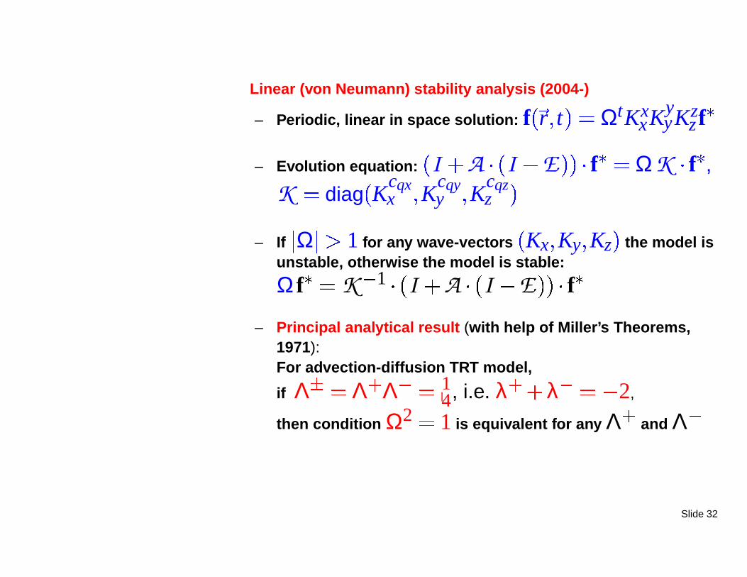
Linear (von Neumann) stability analysis (2004-)
– Periodic, linear in space solution: f r t ΩtKxxKy
yKzz f
– Evolution equation: I A I E f ΩK f ,
K diag Kcqxx K
cqyy K
cqzz
– If
Ω
1 for any wave-vectors Kx Ky Kz the model isunstable, otherwise the model is stable:
Ω f K 1 I A I E f
– Principal analytical result (with help of Miller’s Theorems,1971):For advection-diffusion TRT model,
if Λ Λ Λ 14, i.e. λ λ 2,
then condition Ω2 1 is equivalent for any Λ and Λ
Slide 32

Diffusion dominant criteria for LB:
tx
tz
tz
tx
ty
ty
minimal stencils
– If e
q
tqρ 1 3U2q
U
2
2 , then
αα αα U2α∆t2
LB with Λ Λ 12
MFTCS or Lax-Wendroff
– Positivity of immobile weight: 0 e0ρ 1
– Minimal stencils:e0ρ 1 ∑Q 1
q 1 tq,∆t∆2
x∑d
α 1 αα Λ ∑Q 1q 1 tq
– ∆t and ∆x the model is stable if
Λ
∆t ∑dα 1 αα∆2
x,
– or, ∆t Λ ∆2x
∑dα 1 αα
, Λ
is arbitrary.
– Stability/accuracy is adjusted with Λ Λ 14 .
– LB with Λ Λ 12
Forward-time central scheme (FTCS)
Slide 33
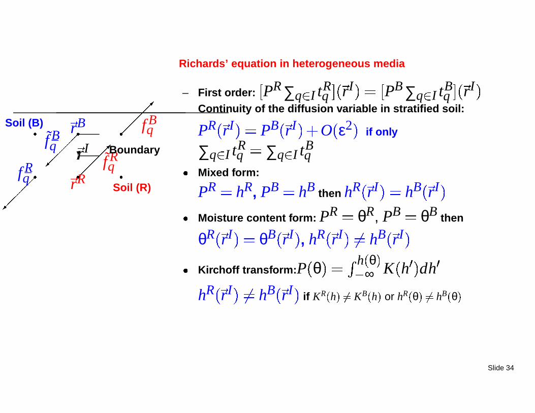
Richards’ equation in heterogeneous media
– First order: PR ∑q I tRq rI PB ∑q I tB
q rI
Continuity of the diffusion variable in stratified soil:
PR rI PB rI O ε2 if only
∑q I tRq ∑q I tB
q
Mixed form:
PR hR, PB hB then hR rI hB rI
Moisture content form: PR θR, PB θB then
θR rI θB rI , hR rI hB rI
Kirchoff transform:P θ
h θ ∞ K h dh
hR rI hB rI if KR h KB h or hR θ hB θ
rR
rB
rIf Rq
f Bq
f Bq
f Rq
Soil (B)
Soil (R)
Boundary
Slide 34

Drainage tube from Marinelli &Durnford (1998)
– Pressure head at the base(z 0) is reduced from thehydrostatic to theatmospheric value
– medium-grained sand is inthe middle betweenfine-grained sands:
Kmiddles Ktop
s 100
– Mixed LB formulation with∆x 1 150 m, ∆t 1 150h
– Minimum ∆x of the adaptiveimplicit RK method is∆x 10 8 10 7m, ∆t 3h
Pressure, [m] Effective θ Velocity/Ks
t 15 h
0
0.5
1
1.5
2
z, [m
]t 57 h
0
0.5
1
1.5
2
z, [m
]
t 75 h
0
0.5
1
1.5
2
z, [m
] 0 8 0 0 6 0 1 2 0
Slide 35

Anisotropic weights (TRT-A) or Anisotropic eigenvalues (LM-I)
– TRT-A :isotropic Λ
q Λ, q
anisotropic weights tq
PR rI PB rI if only
Λ B
Λ R
Bzz
Rzz
– LM-I :isotropic weights:
tRq tB
q cet
q , qanisotropic Λ
q
Exact only if
Λ qB
Λ qR
Bzz
Rzz
– No interface layers if only TqR∂qPR Tq
B∂qPB, Tq Λ q tqVertical flow, necessary: Tq
B
T Rq tqΛ q B
tqΛ q R Bzz R
zz
0 0,5 1 1,5 2
Pressure head h, [m]0
0,5
1
1,5
2
2,5
3
Ele
vati
on
Z,
[m]
TRT-A: discontinuous
e.g, Λ B Λ R
hR rI hB rI
Bzz
Rzz 5
0 0,005 0,01 0,015 0,02 0,025 0,03
Interface layer, [m]0
0,5
1
1,5
2
2,5
3
Ele
vati
on
Z,
[m]
LM-I: correction to solutione.g., diagonal links: T B
q T Rq T R
,
vertical links:T B
T R
7
Slide 36

Anisotropic heterogeneous stratified 3D boxfollowing M. Bakker & K. Hemker, Adv. Water. Res. 2004
Anisotropic principalxy axis:
K i
xx K i
xy 0
K i
xy K i
yy 0
0 0 K i
zz
qx 0qx 0
qz 0
qz 0∂yh σ
– Problem: ∇ KR∇hR 0, z 0, ∇ KB∇hB 0, z 0
– Interface conditions: hR 0 hB 0 , KRzz∂zhR 0 KB
zz∂zhB 0
– Boundary conditions:qx Kxx∂xh Kxy∂yh X 0, ∂yh Y σ, qz Kzz∂zh Z 0
– From 3D to 2D: h x y z φ x z σy hr, hr h 0 0 0 ,∂xφ i X g i , g i K i
xy K i
xx σ
– Three solutions can be distinguished for 2 layered system:Invariant along x and z: φ x z 0, if gB gR 0Linear along x, invariant along z: φ x z gB gR
2 x, if gB gR
Non-linear: φ x z gB gR
2 x gB gR φ x z , if gB gR,∂xφ X z 1
2sign z
Slide 37

Ground water whirls:
u x z K i
xx ∂xφ K i
zz ∂zφ
Isotropic tensors
-1
-0.75
-0.5
-0.25
0
0.25
0.5
0.75
1
-3 -2 -1 0 1 2 3
Ver
tical
coo
rdin
ate
Z
Horizontal coordinate X
Proportional, KBαα KR
αα 5
-1
-0.75
-0.5
-0.25
0
0.25
0.5
0.75
1
-3 -2 -1 0 1 2 3
Ver
tical
coo
rdin
ate
Z
Horizontal coordinate X
Horizontal, KBxx KR
xx 5
-1
-0.75
-0.5
-0.25
0
0.25
0.5
0.75
1
-3 -2 -1 0 1 2 3
Ver
tical
coo
rdin
ate
Z
Horizontal coordinate X
Vertical, KBzz KR
zz 5
-1
-0.75
-0.5
-0.25
0
0.25
0.5
0.75
1
-3 -2 -1 0 1 2 3V
ertic
al c
oord
inat
e Z
Horizontal coordinate X
– Analytical solution (2005) viaFourier series for φ x z KR
xx∂xxφ KRzz∂zzφ 0, z 0
KBxx∂xxφ KB
zz∂zzφ 0, z 0
KRxx KB
xx and KRzz KB
zz
– Boundary:
∂xφ X z
12sign z
∂zφ x Z 0
– Interface:
φ x 0 φ x 0
KBzz∂zφ x 0
KRzz∂zφ x 0
Slide 38
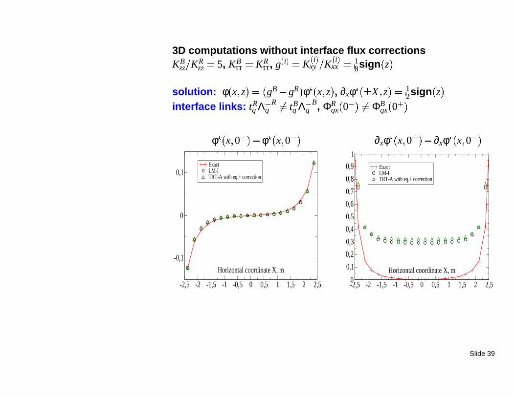
3D computations without interface flux correctionsKB
zz KRzz 5, KB
ττ KRττ, g i K i
xy K i
xx 18sign z
solution: φ x z gB gR φ x z , ∂xφ X z 12sign z
interface links: tRq Λ q
R
tBq Λ q
B, ΦRqx 0 ΦB
qx 0
-2,5 -2 -1,5 -1 -0,5 0 0,5 1 1,5 2 2,5
Horizontal coordinate X, m
-0,1
0
0,1ExactLM-I TRT-A with eq.+ correction
φ x 0 φ x 0 -2,5 -2 -1,5 -1 -0,5 0 0,5 1 1,5 2 2,5
Horizontal coordinate X, m0
0,1
0,2
0,3
0,4
0,5
0,6
0,7
0,8
0,9
1
ExactLM-I TRT-A with eq.+ correction
∂xφ x 0 ∂xφ x 0
Slide 39
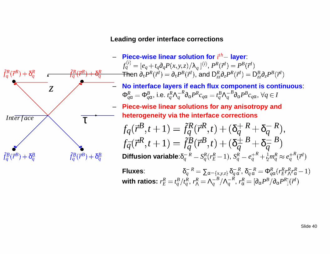
Leading order interface corrections
f Rq rR δR
q
f Bq rB δB
q
f Rq rR δR
q
f Bq rB δB
q
τ
z
Inter f ace
– Piece-wise linear solution for ith layer:f i
q eq tq∂qP x y z λ q i , PR rI PB rI
Then ∂τPR rI ∂τPB rI , and Rzz∂zPR rI B
zz∂zPB rI
– No interface layers if each flux component is continuous:ΦR
qα ΦBqα, i.e. tR
q Λ qR∂αPRcqα tB
q Λ qB∂αPBcqα, q I
– Piece-wise linear solutions for any anisotropy andheterogeneity via the interface corrections
fq rB t 1 f Rq rR t δ R
q δ Rq ,
fq rR t 1 f Bq rB t δ B
q δ Bq
Diffusion variable:δ Rq SR
q rRE
1 , SRq e
qR
12mR
q e
qR rI
Fluxes: δ Rq ∑α x y z
δ Rq α , δ R
q α ΦRqα rR
ErRΛrR
α 1
with ratios: rRE tB
q tRq , rR
Λ Λ qB
Λ qR, rR
α ∂αPB
∂αPR rI
Slide 40

LM-I-model with interface correctionsComparison with exact and “multi-layer” solutions for
∂xφ B x 0 and ∂xφ R x 0
, K i
xy K i
xx sign z 2– Neumann conditions via the
modified bounce-back:fq rb t 1
fq rb t δn rb t δτ rb t
– Prescribed normal derivative:δn 2Tq∂nP rw t Cqn
– Relaxed tangentialderivatives:δτ 2Tq ∑τ ∂τP rb t Cqτ,∂τP is derived from thecurrent population solution
-2,5 -2 -1,5 -1 -0,5 0 0,5 1 1,5 2 2,5Horizontal coordinate X
-0,5
-0,25
0
0,25
0,5
Exact2D multi-layer2D LM-I3D LM-I
KBzz KR
zz 500, KBττ KR
ττdiagonal links:
T Bd1 T R
d1
T Rd2 T B
d2
7vertical links: T B
T R
1498
-2,5 -2 -1,5 -1 -0,5 0 0,5 1 1,5 2 2,5Horizontal coordinate X
-0,5
-0,25
0
0,25
0,5
Exact2D multi-layer2D LM-I3D LM-I
KBzz KR
zz 500, KBττ KR
ττ 100diagonal links:
T Bd1 T R
d1
T Rd2 T B
d2
100vertical links: T B
T R
1300
Slide 41
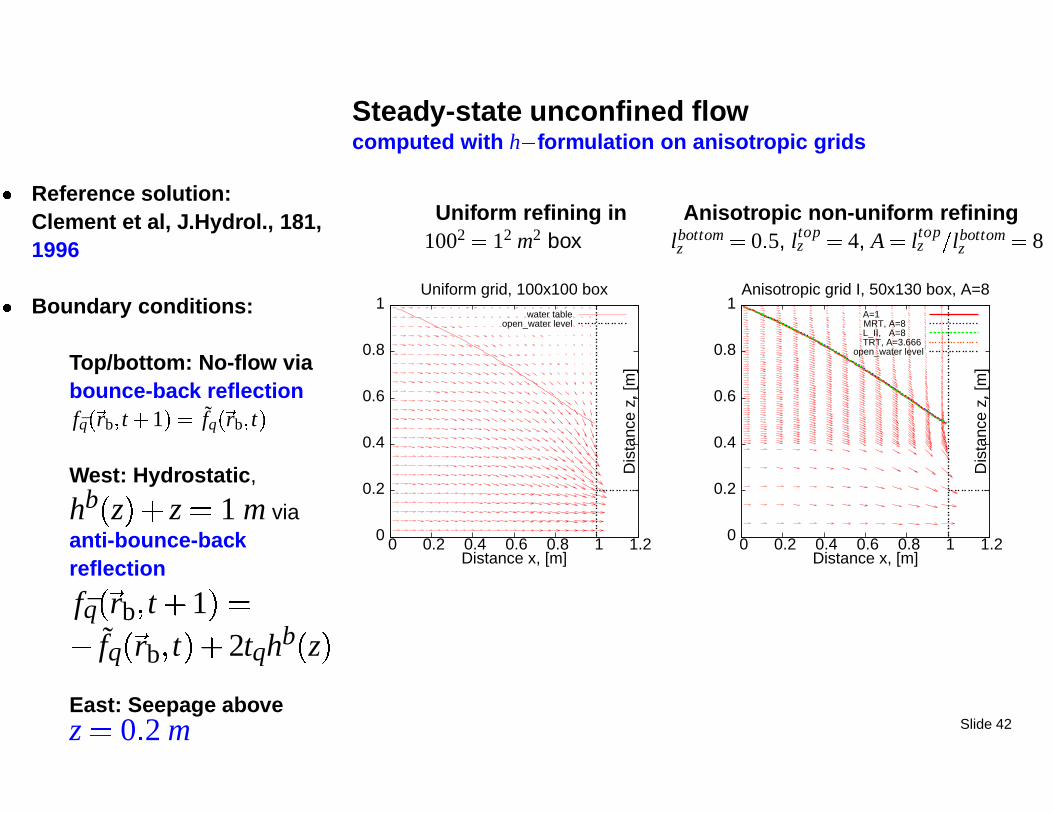
Steady-state unconfined flowcomputed with h formulation on anisotropic grids
Uniform refining in1002 12 m2 box
0
0.2
0.4
0.6
0.8
1
0 0.2 0.4 0.6 0.8 1 1.2
Dis
tanc
e z,
[m]
Distance x, [m]
Uniform grid, 100x100 boxwater table
open_water level
Anisotropic non-uniform refininglbottomz 0 5, ltop
z 4, A ltopz lbottom
z 8
0
0.2
0.4
0.6
0.8
1
0 0.2 0.4 0.6 0.8 1 1.2
Dis
tanc
e z,
[m]
Distance x, [m]
Anisotropic grid I, 50x130 box, A=8A=1 MRT, A=8 L_II, A=8 TRT, A=3.666
open_water level
Reference solution:Clement et al, J.Hydrol., 181,1996
Boundary conditions:
Top/bottom: No-flow viabounce-back reflectionfq rb t 1 fq rb t
West: Hydrostatic,
hb z z 1 m viaanti-bounce-backreflection
fq rb t 1
fq rb t 2tqhb z
East: Seepage abovez 0 2 m Slide 42
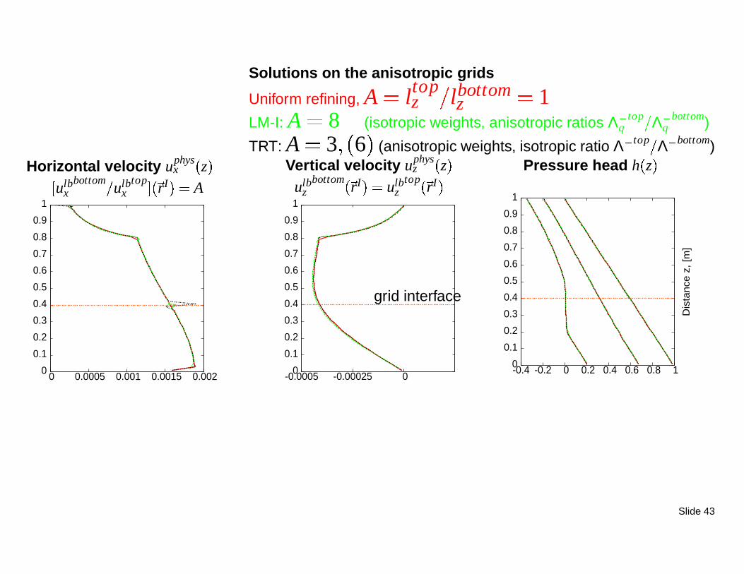
Solutions on the anisotropic grids
Uniform refining, A ltopz lbottom
z 1LM-I: A 8 (isotropic weights, anisotropic ratios Λ q
top
Λ qbottom)
TRT: A 3 6 (anisotropic weights, isotropic ratio Λ top
Λ bottom)Vertical velocity uphys
z z
ulbz
bottom rI ulbz
top rI
0
0.1
0.2
0.3
0.4
0.5
0.6
0.7
0.8
0.9
1
-0.0005 -0.00025 0
grid interface
Pressure head h z
0
0.1
0.2
0.3
0.4
0.5
0.6
0.7
0.8
0.9
1
-0.4 -0.2 0 0.2 0.4 0.6 0.8 1
Dis
tan
ce z
, [m
]
Horizontal velocity uphysx z ulb
xbottom
ulbx
top rI A
0
0.1
0.2
0.3
0.4
0.5
0.6
0.7
0.8
0.9
1
0 0.0005 0.001 0.0015 0.002
Slide 43

AADE: interface collision operator (2005)
– Prescribed continuity conditions:
Diffusion variable: e Rq rI e B
q rI O ε2
Advective-diffusive flux components:e R
q
Λ qRmR
q e Bq
Λ qBmB
q
– Interface collision components:
(1) e Iq 1
2 e Rq e B
q
Harmonic means:
LM-I : Λ Iq 2Λ q
BΛ qR
Λ qB Λ q
R if Λ qR
Λ qB mB
q mRq
TRT-A: Λ I 2Λ BΛ R
Λ B Λ R if Λ R
Λ B ∑q I mBq ∑q I mR
q
(2) pIq 1
2 pRq pB
q (3) Mass source: Q I
q 12 Q R
q Q Bq
(4) Deficiency: PI 12 P R P B ∆P, ∆P 1
4 ∂zP B ∂zP R
-1 -0,8 -0,6 -0,4 -0,2 0 0,2 0,4 0,6 0,8 1Channel width, m
0
2
4
6
8
10
12
h z h 0
Harmonic mean:
KIzz 2KR
zzKBzz
KRzz KB
zzifΛ q
R
Λ qB Λ R
Λ B KRzz KB
zz
With or without convection:∇ K∇ h
1g 0 or∇ K∇h 0 Slide 44
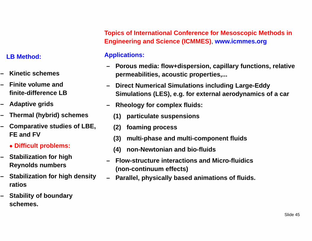
Topics of International Conference for Mesoscopic Methods inEngineering and Science (ICMMES), www.icmmes.org
LB Method:
– Kinetic schemes
– Finite volume andfinite-difference LB
– Adaptive grids
– Thermal (hybrid) schemes
– Comparative studies of LBE,FE and FV
Difficult problems:
– Stabilization for highReynolds numbers
– Stabilization for high densityratios
– Stability of boundaryschemes.
Applications:
– Porous media: flow+dispersion, capillary functions, relativepermeabilities, acoustic properties,...
– Direct Numerical Simulations including Large-EddySimulations (LES), e.g. for external aerodynamics of a car
– Rheology for complex fluids:
(1) particulate suspensions
(2) foaming process
(3) multi-phase and multi-component fluids
(4) non-Newtonian and bio-fluids
– Flow-structure interactions and Micro-fluidics(non-continuum effects)
– Parallel, physically based animations of fluids.
Slide 45
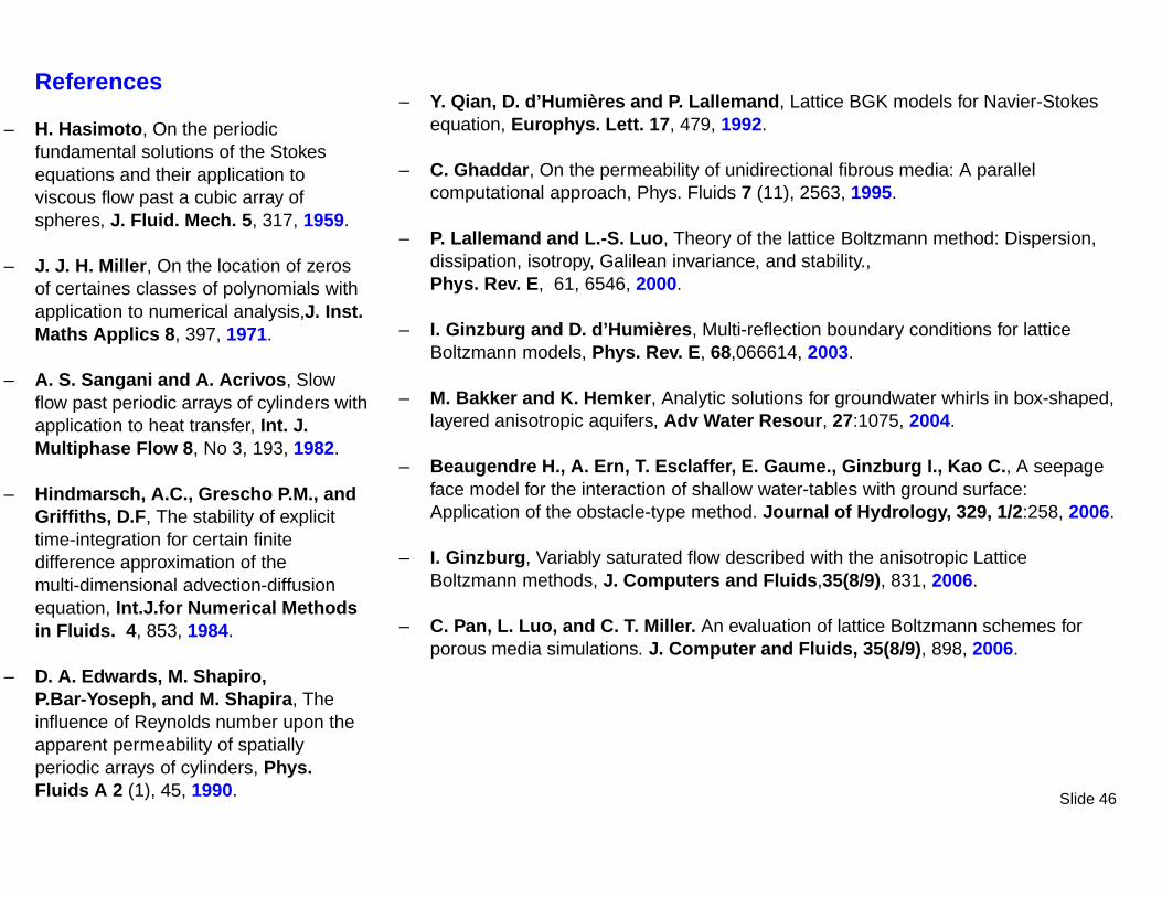
References
– H. Hasimoto, On the periodicfundamental solutions of the Stokesequations and their application toviscous flow past a cubic array ofspheres, J. Fluid. Mech. 5, 317, 1959.
– J. J. H. Miller, On the location of zerosof certaines classes of polynomials withapplication to numerical analysis,J. Inst.Maths Applics 8, 397, 1971.
– A. S. Sangani and A. Acrivos, Slowflow past periodic arrays of cylinders withapplication to heat transfer, Int. J.Multiphase Flow 8, No 3, 193, 1982.
– Hindmarsch, A.C., Grescho P.M., andGriffiths, D.F, The stability of explicittime-integration for certain finitedifference approximation of themulti-dimensional advection-diffusionequation, Int.J.for Numerical Methodsin Fluids. 4, 853, 1984.
– D. A. Edwards, M. Shapiro,P.Bar-Yoseph, and M. Shapira, Theinfluence of Reynolds number upon theapparent permeability of spatiallyperiodic arrays of cylinders, Phys.Fluids A 2 (1), 45, 1990.
– Y. Qian, D. d’Humières and P. Lallemand, Lattice BGK models for Navier-Stokesequation, Europhys. Lett. 17, 479, 1992.
– C. Ghaddar, On the permeability of unidirectional fibrous media: A parallelcomputational approach, Phys. Fluids 7 (11), 2563, 1995.
– P. Lallemand and L.-S. Luo, Theory of the lattice Boltzmann method: Dispersion,dissipation, isotropy, Galilean invariance, and stability.,Phys. Rev. E, 61, 6546, 2000.
– I. Ginzburg and D. d’Humières, Multi-reflection boundary conditions for latticeBoltzmann models, Phys. Rev. E, 68,066614, 2003.
– M. Bakker and K. Hemker, Analytic solutions for groundwater whirls in box-shaped,layered anisotropic aquifers, Adv Water Resour, 27:1075, 2004.
– Beaugendre H., A. Ern, T. Esclaffer, E. Gaume., Ginzburg I., Kao C., A seepageface model for the interaction of shallow water-tables with ground surface:Application of the obstacle-type method. Journal of Hydrology, 329, 1/2:258, 2006.
– I. Ginzburg, Variably saturated flow described with the anisotropic LatticeBoltzmann methods, J. Computers and Fluids,35(8/9), 831, 2006.
– C. Pan, L. Luo, and C. T. Miller. An evaluation of lattice Boltzmann schemes forporous media simulations. J. Computer and Fluids, 35(8/9), 898, 2006.
Slide 46
![DYNAMICS OF THE GINZBURG-LANDAU EQUATIONS OF/67531/metadc...1.1 Ginzburg-Landau Model of Superconductivity In the Ginzburg-Landau theory of phase transitions [3], the state of a super-](https://static.fdocuments.in/doc/165x107/60a17031f8ca2108311ab385/dynamics-of-the-ginzburg-landau-equations-of-67531metadc-11-ginzburg-landau.jpg)