1

Invitation to the 2015 “Blind test 4” Workshop Combined power output of two in-line turbines at different inflow conditions

Lars Sætran and Jan Bartl

Department of Energy and Process Engineering, NTNU, Trondheim, Norway

Contact: lars.satran@ntnu.no, jan.bartl@ntnu.no

Abstract:

This note describes a 4th blind test case organized by NOWITECH and NORCOWE. We invite you to submit predictions for the described test cases and participate in a two-day workshop to be held in Trondheim, scheduled for October 2015. Here, the results from the predictions will be discussed and a comparison with measurements will be presented. Schedule: • March 27th, 2015: Blind test invitation sent out • Oct. 1st, 2015: Deadline for submission of simulation results • End of Oct, 2015: Blind test workshop in Trondheim (you will be informed about the exact

dates later)

Background: BT1: The first blind test, BT1, was organized in Bergen, in October 2011, and attracted

around 40 participants with 11 sets of predictions being submitted. For that blind test the geometry of a model turbine was made available and the participants were asked to predict its performance and the wake development from the turbine down to 5 diameters. The results from BT1 have been reported in [1].

BT2: For the next blind test, held in Trondheim, in October 2012, the test complexity was

increased by adding a downstream turbine behind the upstream turbine. The main task in BT2 was to predict the performance of the downstream turbine, which is affected by the wake developing behind the upstream turbine. The participants were also asked to predict the flow in the wake behind the downstream turbine. Obviously, this was a more complicated test case than BT1 and required more computer resources to be performed properly. Despite this, results were submitted by 9 different participants. The results were reported in [2].

BT3: For the third blind test, BT3, the complexity was slightly increased again. The same

turbines were used, positioned with the same streamwise separation, but shifted slightly sideways so that the wake from the upstream turbine only hit a part of the rotor plane of the downstream turbine. In this way the downstream turbine experienced an asymmetric load. Also, the wake development behind the downstream turbine was no longer axisymmetric. The tests were performed in a virtually turbulence free, uniform flow environment, as well as in a turbulent flow. In the latter case a grid was installed at the wind tunnel inlet producing a uniform inflow with about 10% turbulence intensity at the location of the upstream turbine. The results from the BT3 were reported in [3].

Motivation:

Given the constraints of transmission and installation costs, the available area for offshore wind farm installations is fairly limited. Under these circumstances, the wake effect plays a key role when evaluating the energy production since the energy captured by a wind turbine leads to a

2

decrease of the wind speed downstream. As a result, wind turbines located downstream produce less energy than if they were in the unobstructed free stream. In the case of onshore wind farms, the energy losses due to the wake effect constitute about 5 - 10% of the production [4], while in offshore wind farms, the wake effect losses can reach higher values; approximately 15% [5]. During the design stage of a wind farm, and in order to increase the wind farm production (by reducing wind speed deficits or wake effect losses), it would be desirable to separate the wind turbines as far as possible. However, due to constraints such as space availability and cost of electrical connections and the total cost of electrical losses over the lifespan of the installation the maximum distance between the individual wind turbines is limited [6].

The concept of individual power control of wind turbines was initially suggested by Steinbuch et al. [7] by selecting the tip speed ratio of each wind turbine by means of trial and error. In 2004, Corten and Schaak [8] presented experimental results showing the possibility of increasing the power generated and of reducing the loads by individually selecting the tip speed ratio of each wind turbine. In early 2011, Larsen et al. [9] presented the technical report corresponding to the TOPFARM project which deals with optimal topology design and control of wind farms. That study showed that it is possible to increase the overall efficiency of a wind farm through the individual control of the generated power by each wind turbine. In 2012 Lee et al. [10] presented a strategy of individual control of each of the wind turbines by optimizing the pitch angle of each turbine by means of a genetic algorithm, and used a wake model based on the eddy viscosity model. In that study, the authors considered the case of a row of wind turbines and achieved an improvement in the aerodynamic power of 4.5% with regard to the conventional operating strategy.

1 The BT4 test case definitions BT4: In this fourth blind test we are focusing on the total power output from two in-line turbines. We use the same turbines as used in the previous BTs and study the influence of inlet conditions and turbine separation distance on the combined power performance of the two turbines.

The axial separation distance between the turbines is set x/D = 2.77, x/D = 5.18 and x/D = 9.00. Furthermore, we are able to provide three different inflow conditions at the inlet to the test section: • Low turbulence uniform inflow: No grid at the inlet to the test section. At the

position of the upstream turbine the turbulence intensity measured is TI= 0.23%. The mean wind speed is uniform across the test section, apart from small wall boundary layer effects.

• High turbulence uniform inflow: An evenly spaced turbulence gird at the tunnel inlet generates a higher turbulence intensity level of TI= 10.0% at the location of the upstream turbine. The mean wind speed is uniform across the test section.

• High turbulence shear inflow: A turbulence grid with increasing vertical distance between the horizontal bars is installed at the inlet of the test section. This is creating a non-uniform shear flow with a mean turbulence intensity of TI=10.1% over the rotor swept area of the upstream turbine.

In the following we provide detailed information about the setup of the different test

cases. Depending on whether your computational model assumes axisymmetric flow and uses a rotating frame of reference, or computes a rotating rotor in a fixed environment, you may want to use the exact tunnel dimensions or convert the cross section to an equivalent circular cylinder in order to account for possible blockage effects and wall boundary layers. Furthermore, we provide full details of the model geometry. A CAD file that describes one blade mounted on one third of the nacelle is available. Alternatively, it is possible to build your own geometry from tables containing definitions of the airfoil, as

3

well as the chord length and twist as function of the radius. All information needed is described in the following sections.

1.1 The models

A picture of the turbine models installed in the wind tunnel is shown in Figure 1. Both turbines have three bladed upstream rotors with exactly the same blade geometry, but a slightly different total rotor diameter, due to different nacelle geometries. The blades were machined in aluminum and have a NREL S826 airfoil section from root to tip. (See: Somers [11] for the full airfoil documentation.)

Figure 1: Model wind turbines in the wind tunnel (x/D=9.00)

In Figure 2 the dimensions of the two turbines are defined indicating that the models

have slightly different tower and nacelle layouts. Note that the tower heights given in the figure show their physical dimensions to the fixing points below the wind tunnel floor and not their actual height as operated in the wind tunnel. These heights will be specified further down.

The upstream turbine will in the following be referred to as T1, while T2 is defined to be the downstream turbine. The two turbines are positioned at three streamwise separation distances of 2.77D, 5.18D and 9.00D, where D is defined as D = D T 2 = 0.894m. This is the diameter of the rotor of the downstream turbine T2.

The tower of turbine T1 is a cylinder with a constant diameter of DT o w, T 1= 0.11m, while for T2 the rotor sits on top of a stepped tower consisting of 4 cylinders of different diameters. T2 is the same turbine that was used in BT1 [1]. The nacelle of turbine T1 is a circular cylinder of DNac,T1

= 0.130m diameter. The nacelle of T2 is also circular but with a diameter of DNac,T1

= 0.130m. The rotor diameter of T1 is DT1 = 0.944m, while DT2 = 0.894m. The individual blades have a total length of lBlade = 0.413m and are directly mounted on the hubs with the diameters Dhub,T1

= 0.118m and Dhub,T2 = 0.068m.

Both turbines are driven by a belt transmission connected to a 0.37kW asynchronous motor located under the tunnel floor. Turbine T1 has the belt mounted inside the tower, while for T2 the tower is too slender to allow this, so the belt runs behind the turbine tower.

Turbine T2 has an almost semi- spherical hub cover at the front. Its deviation from a sphere is small but if the exact geometry is deemed necessary, it may be obtained from the organizers as a table in an Excel file. In the CAD file mentioned above, the correct shape is of course included. At the rear, the cap is again formed from a sphere, slightly offset and with a somewhat larger diameter, as indicated in the figure. Turbine T1 has a slightly pointed hub cover. The dimensions are documented in Figure 2(a); a CAD file and an excel file are available for download for this turbine, too. Both turbines rotate in the counter-clockwise direction with the observer standing upstream and looking in flow direction.

4

Figure 2 (a): Tower and nacelle dimensions of the upstream turbine T1

Figure 2 (b): Tower and nacelle dimensions of the downstream turbine T2

5

Figure 3: Turbine positions in the wind tunnel and reference coordinate system

Figure 4: Wind tunnel test section from above and reference coordinate system

6

1.2 The blade geometry

The NREL S826 airfoil is used along the entire blade span. The normalized coordinates for the profile are given in Section 2. We also include a table of chord length and twist angle as function of the radius, which you will find in Section 3. Combined, this information allows you to define the blade geometry.

Furthermore, we supply a CAD file containing a 120 degrees segment of the nacelle of turbine T2 with one blade mounted in the correct position as well as the complete 3D CAD files of both model turbines.

The CAD files may be downloaded from: http://www.ivt.ntnu.no/ept/downloads/workshop2015 The login details are: User: Workshop2015 Password: Turbine

1.3 The test environment

The model turbines were tested in a closed- return wind tunnel. It has a test section which is 2.71m wide and 11.15m long. The tunnel has a flexible roof which has been adjusted for zero pressure gradient at 10m/s. The tunnel heights are given in Table 1.

X (m) Height (m) 0.000 2.810 5.621 8.435

11.150

1.801 1.801 1.813 1.842 1.851

Table 1: Height of test section as function of distance from the inlet

Both turbines were installed such that they have the same rotor axis height above the wind tunnel floor, hhub = 0.827m (see Figure 3). All measurements were taken with a bulk velocity at the test section inlet equal to U∞ = 11.5m/s. In the turbulent shear inflow case, the reference velocity at the rotor axis height hhub = 0.827m was set to Uref,hub = 11.5m/s. The design tip speed ratio for both the upstream and downstream turbine is λ = ΩR/U∞ = 6. At the design condition this gives a Reynolds number of Rec = λ Uctip/ν ≈ 105 , where ctip is the chord length at the blade tip and ν the kinematic viscosity of air.

At the inlet to the empty test section the flow is uniform across the cross section to within ±1%, except for the thin region of wall boundary layers, and the turbulence intensity was been measured to be 0.23%. The conventional model which relates the dissipation rate of turbulent kinetic energy, E, to the streamwise velocity fluctuation, u, and the streamwise integral length scale, Luu, is given by

3

E = A 2

u3

Luu

(1)

7

2

Using 3 A ≈ 1 (taken from Krogstad and Davidson, [12]) the integral length in the streamwise direction at the test section inlet was calculated from measurements of u and E to be Luu = 0.035m when no grid was set up at the inlet. (Note that this length is virtually identical to the length scale obtained by integrating the streamwise auto-correlation function normally specified. However, this integral quantity is experimentally much harder to measure correctly and was therefore not used here.)

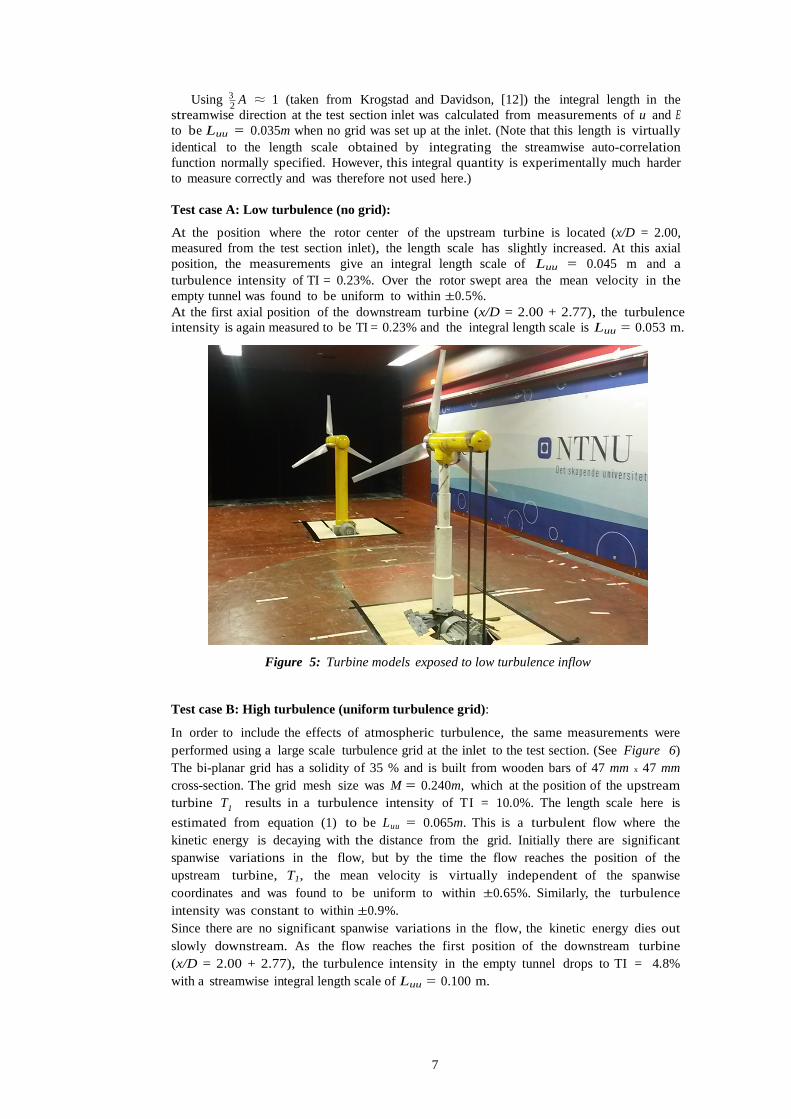
Test case A: Low turbulence (no grid): At the position where the rotor center of the upstream turbine is located (x/D = 2.00, measured from the test section inlet), the length scale has slightly increased. At this axial position, the measurements give an integral length scale of Luu = 0.045 m and a turbulence intensity of TI = 0.23%. Over the rotor swept area the mean velocity in the empty tunnel was found to be uniform to within ±0.5%. At the first axial position of the downstream turbine (x/D = 2.00 + 2.77), the turbulence intensity is again measured to be TI = 0.23% and the integral length scale is Luu = 0.053 m.

Figure 5: Turbine models exposed to low turbulence inflow

Test case B: High turbulence (uniform turbulence grid): In order to include the effects of atmospheric turbulence, the same measurements were performed using a large scale turbulence grid at the inlet to the test section. (See Figure 6) The bi-planar grid has a solidity of 35 % and is built from wooden bars of 47 mm x 47 mm cross-section. The grid mesh size was M = 0.240m, which at the position of the upstream turbine T1 results in a turbulence intensity of TI = 10.0%. The length scale here is estimated from equation (1) to be Luu = 0.065m. This is a turbulent flow where the kinetic energy is decaying with the distance from the grid. Initially there are significant spanwise variations in the flow, but by the time the flow reaches the position of the upstream turbine, T1, the mean velocity is virtually independent of the spanwise coordinates and was found to be uniform to within ±0.65%. Similarly, the turbulence intensity was constant to within ±0.9%. Since there are no significant spanwise variations in the flow, the kinetic energy dies out slowly downstream. As the flow reaches the first position of the downstream turbine (x/D = 2.00 + 2.77), the turbulence intensity in the empty tunnel drops to TI = 4.8% with a streamwise integral length scale of Luu = 0.100 m.

8

Figure 6: Turbine models exposed to high turbulence inflow generated by an evenly spaced

grid

Test case C: High turbulence shear flow (shear flow turbulence grid): In a third test case the effect of shear flow in an atmospheric boundary layer combined with atmospheric turbulence is investigated. The same measurement series, as for the other test cases, were performed using a large scale shear flow turbulence grid at the inlet to the test section. (See Figure 7)

Figure 7: Turbine models exposed to highly turbulent shear flow

The horizontal mesh width is 0.240m, while the vertical mesh heights vary between 0.0165m near the floor and 0.300 m underneath the roof. The grid is bi-planar and has a solidity of 38%. As for the evenly spaced turbulence grid, it is built from wooden bars of 47 mm x 47 mm cross-section. The exact positions of the horizontal bars are documented in Table 2:

9

Table 2: Positions of the horizontal bars in the shear grid, measured at the bar center.

At the position of the upstream turbine, T1 , a turbulence intensity of 10.1% is measured ta the hub height. The turbulent length scale at the height of the nacelle h=0.827m is estimated to be Luu = 0.097m. The kinetic energy in the flow is decaying with the distance from the grid. At the first position of the downstream turbine (x/D = 2.00 + 2.77) the turbulence intensity has decayed to TI = 5.2% and the length scale grown to Luu = 0.167m. At the second downstream position (x/D = 2.00 + 5.18) a turbulence intensity of 4.1% and a Luu = 0.271m is measured. At the third downstream position (x/D = 2.00 + 9.00) the turbulence intensity has decayed to TI = 3.7% while the length scale has grown to Luu = 0.318m. As wind shear and turbulence are generated only at the grid position at the tunnel inlet, their development throughout the tunnel is measured at all four turbine positions. A common way to describe atmospheric wind shear is the power law, which expresses the wind speed, U, as function of height, z, provided that the wind speed at an arbitrary reference height, zref, is known:

U(z) = (

z )α U(zref) zref

(2)

The power law coefficient α describes the strength of shear in the wind profile. A wind profile based on a shear coefficient of α=0.11 was chosen as a reference for this study, and the shear generating grid was designed to imitate this specific wind profile. Figure 8 shows the mean wind speed, U, as function of the height z, as well as the turbulence intensity measured in the empty tunnel at the positions of the upstream turbine T1 (xT1 = 2.00D) and the downstream turbine (xT2,5D = 2.00D + 2.77D ≈ 5D // xT2,7D = 2.00D + 5.18D ≈ 7D // xT2,11D = 2.00D + 9.00D ≈ 11D).

Figure 8: Measured mean wind speed and turbulence intensity at all measurement locations for turbulent shear inflow

Bar no. Height of bar center above the wind tunnel floor [mm]

8 1600 7 1300 6 1015 5 795 4 575 3 385 2 203 1 40

10

2 Definition of the NREL S826 airfoil

The definitions of the NREL S826 airfoil used for the blade can be found in Somers [11] and the airfoil is shown in Figure 9. Table 3 contains a list of the normalized coordinates for the airfoil. Somers specifies the geometry, as well as estimated performance characteristics, such as lift and drag coefficients, for a range of full scale operating Reynolds numbers. Unfortunately, these are computed for much higher Re than the ones applicable in the model tests.

Figure 9: Shape of the NREL S628 airfoil

For the first two blind tests, the participants were asked to estimate the performance

data for S826 themselves. When the predictions were analyzed and compared, we have seen that part of the scatter in the results may be traced back to the fact that different groups have generated quite different estimates for the lift and drag coefficients. We have decided to reduce the uncertainty of different airfoil coefficients and therefore provide a standard set of CL and CD coefficients that the participants should use for all operating conditions. Thus, some scatter in the predictions may disappear, possibly at the expense of introducing some systematic differences between the predictions and the measurements.

The data to be used is presented in Table 4. Note that this set is given for one Reynolds number only (Rec = 105). This corresponds to the Rec obtained at the blade tip at the design operating condition, i.e. at a tip speed ratio of 6. Obviously, this will be somewhat incorrect for the inner part of the blade, but the effects on the performance data at the design condition have been seen to be small. In Figure 10 the data from Table 4 are compared with 2D measurements on the S826 performed at DTU, Denmark, [13] and at METUWIND, Turkey. The XFOIL data in Table 4 are seen to fall between the measurements, capturing the trends from the METUWIND at the normal operating modes, but being closer to the DTU data at extremely high angles of attack. Measurements for Rec = 105 are shown, but more data are available from both DTU’s and the METUWIND’s measurement campaigns.

Figure 10: Comparison of CL/CD datasets [13]

11

If you are insisting on using lift and drag data at the correct Re as it varies with radial position and turbine operating conditions, you will need to generate your own data tables. You can do this by using the program package called XFOIL ( see Drela [14]) or obtain the complete measurement data sets directly from DTU or METUWIND. (Contact information can be provided upon request.) It is important that you inform us about how the information is obtained if you do not use the data provided here.

x/c y/c (upper surface) x/c y/c (lower surface)

0.0000 0.00018000 0.0025500 0.0095400 0.020880 0.036510 0.056360 0.080260 0.10801 0.13934 0.17395 0.21146 0.25149 0.29361 0.33736 0.38228 0.42820 0.47526 0.52324 0.57161 0.61980 0.66724 0.71333 0.75749 0.79915 0.83778 0.87287 0.90391 0.93072 0.95355 0.97251 0.98719 0.99668 1.0000

0.0000 0.0015900 0.0074800 0.016380 0.025960 0.035800 0.045620 0.055190 0.064340 0.072880 0.080680 0.087580 0.093430 0.098070 0.10133 0.10294 0.10249 0.10005

0.096070 0.090940 0.084890 0.078160 0.070950 0.063410 0.055720 0.047980 0.040290 0.032620 0.024790 0.016950

0.0098200 0.0043100 0.0010300

0.0000

0.0000 0.00021000 0.00093000 0.0021600 0.0036700 0.013670 0.029200 0.049980 0.075800 0.10637 0.14133 0.17965 0.21987 0.26153 0.30497 0.35027 0.39779 0.44785 0.50032 0.55484 0.61055 0.66644 0.72142 0.77434 0.82409 0.86953 0.90945 0.94257 0.96813 0.98604 0.99655 1.0000

0.0000 -0.0014600 -0.0027400 -0.0040300 -0.0052500 -0.010350 -0.015180 -0.019600 -0.023620 -0.027290 -0.030910 -0.034860 -0.038550 -0.040640 -0.040510 -0.037940 -0.032800 -0.025630 -0.017200

-0.0084100 -0.0001500 0.0069900 0.012540 0.016210 0.017840 0.017410 0.014980 0.011130

0.0068900 0.0032400 0.0008400

0.0000

Table 3: Coordinates for the NREL S826 airfoil

α CL CD CL /CD α CL CD CL /CD -40.0 -35.0 -30.0 -25.0 -20.0 -18.0 -16.0 -14.0 -12.0 -11.0 -10.0 -9.00 -8.00 -7.00 -6.00 -5.00 -4.00 -3.00 -2.00 -1.00 0.00 1.00 2.00

-0.96710 -0.87580 -0.75170 -0.60080 -0.43470 -0.36800 -0.30430 -0.24910 -0.20180 -0.18650 -0.18110 -0.19240 -0.25200 -0.23440 -0.14360

-0.049500 0.071400 0.18800 0.30260 0.41360 0.52200 0.62690 0.72880

0.39968 0.36549 0.32383 0.27557 0.22170 0.19869 0.17474 0.14843 0.12244 0.10792

0.091970 0.073190 0.054460 0.038600 0.029050 0.023940 0.021820 0.021090 0.020730 0.020770 0.021040 0.021530 0.022220

-2.4197 -2.3962 -2.3213 -2.1802 -1.9608 -1.8521 -1.7414 -1.6782 -1.6482 -1.7281 -1.9691 -2.6288 -4.6272 -6.0725 -4.9432 -2.0677 3.2722 8.9142 14.597 19.913 24.810 29.118 32.799

3.00 4.00 5.00 6.00 7.00 8.00 9.00 10.0 11.0 12.0 13.0 14.0 15.0 16.0 18.0 20.0 22.0 25.0 30.0 34.0 40.0 50.0

0.82540 0.91800 1.0019 1.0783 1.1469 1.2060 1.2550 1.2929 1.3320 1.3509 1.3718 1.3784 1.3638 1.3431 1.2563 1.1940 1.2493 1.3379 1.4702 1.5519

0.96620 0.84970

0.023250 0.024420 0.025880 0.027800 0.030290 0.033540 0.037850 0.043660 0.049960 0.059220 0.069050 0.081720 0.098800 0.11883 0.17904 0.26157 0.29458 0.33390 0.38800 0.42331 0.63129 0.73405

35.501 37.592 38.713 38.788 37.864 35.957 33.157 29.613 26.661 22.812 19.867 16.867 13.804 11.303 7.0169 4.5647 4.2410 4.0069 3.7892 3.6661 1.5305 1.1576

Table 4: Lift and drag coefficients calculated for Re = 1.0 × 105 using XFOIL.

12

3 Chord and twist data

Table 5 contains a list of the airfoil chord length and twist angle as function of the radius. (The twist angle is measured with respect to the rotor plane.) Please note that for the first 3 coordinate sets the geometry consists of a circular cylinder used to fix the blade to the hub. Therefore a major part of this section is located inside the hub when defining the rotor geometry. This section has been identified in the table by setting the twist angle to 120 degrees. Between the last circular section and the first NREL profile, a linear transition region is giving a smooth change of shape. The blade is shown in Figure 11.

(a)

(b)

Figure 11: Blade (a) seen in the plane of rotation and (b) in the axial direction

Figure 11

c (m) φ (deg) 0.0075000 0.022500 0.049000 0.055000 0.067500 0.082500 0.097500 0.11250 0.12750 0.14250 0.15750 0.17250 0.18750 0.20250 0.21750 0.23250 0.24750 0.26250 0.27750 0.29250 0.30750 0.32250 0.33750 0.35250 0.36750 0.38250 0.39750 0.41250 0.42750 0.44250

0.013500 0.013500 0.013500 0.049500 0.081433 0.080111 0.077012 0.073126 0.069008 0.064952 0.061102 0.057520 0.054223 0.051204 0.048447 0.045931 0.043632 0.041529 0.039601 0.037831 0.036201 0.034697 0.033306 0.032017 0.030819 0.029704 0.028664 0.027691 0.026780 0.025926

120.00 120.00 120.00 38.000 37.055 32.544 28.677 25.262 22.430 19.988 18.034 16.349 14.663 13.067 11.829 10.753 9.8177 8.8827 7.9877 7.2527 6.5650 5.9187 5.3045 4.7185 4.1316 3.5439 2.9433 2.2185 1.0970 -0.7167

Table 5: Definitions of chord length and twist angle as function of blade radius.

13

4 Operating conditions

This section describes the operating configurations for which the computational output may be submitted. For all cases the upstream turbine T1 is located at x = 1788mm measured from the inlet to the test section, which corresponds to a distance of 2.00D. For the test cases A, B and C the downstream turbine T2 is positioned at Δx = 4630mm behind the upstream turbine, which corresponds to 5.18D separation distance. The inflow conditions are varied from low turbulence (A), to high turbulence (B) and high turbulence shear flow (C). For the test cases B1, B2, B3, the inflow condition is set to high turbulence (B) and is not varied. However, here the streamwise separation distance between the turbines is varied from Δx = 2480mm (2.77D, B1) through Δx = 4630mm (5.18D, B2) to Δx = 8046mm (9.00D, B3). This comparison should illustrate the influence of the separation distance on the total efficiency. This makes up a total number of 5 test cases as test case B and B2 are identical. For all test cases the inflow velocity is set to U∞ = 11.5m/s; for the non-uniform shear inflow (test case C) this is the reference inflow velocity at hub height hhub = 0,827m. The blade pitch angle is set to β = 0° for all test cases. The density of air can be assumed to be ρ = 1.20kg/m3.

4.1 Test cases A, B, C: varying inflow conditions

For these test cases the downstream turbine’s position is fixed at Δx = 4630mm (5.18D) behind the upstream turbine. The inflow conditions are varied from low turbulence (A), to high turbulence (B) and high turbulence shear flow (C). A detailed description of the inflow conditions is given in section 3. 4.1.1 Turbine performance CP and thrust CT: The upstream turbine T1 is operated at a tip speed ratio of λT1 = ΩR/U∞= 6.0, whereas the downstream turbine T2 is run at λT2 = ΩR/U∞ = 4.5. Note, that the same reference velocity U∞ is used for both turbines. For each inlet condition A, B and C,

1. the power coefficients CP,T1 and CP,T2 as well as 2. the thrust coefficients CT,T1 and CT,T2

should be presented at these operating points. The thrust coefficients should be calculated for the rotor only, i.e. the contribution of the tower to the thrust must not be taken into account.

4.1.2 Horizontal wake profiles Furthermore, the horizontal wake profile at Δx = 2480mm (2.77D) behind the upstream turbine T1 should be documented at λT1 = 6.0 for the three inlet conditions A, B and C. This is an axial position in between the two turbines. A profile of the

1. normalized mean velocity U/U∞ as well as the 2. normalized turbulent kinetic energy k* = k/U∞

should be presented. Profiles along a horizontal line at the elevation of the center of the turbine hub (hhub = 0.827 m) should be extracted covering the horizontal span width from z = -944mm (-2 RT1) to z = +944mm (+2 RT1). For the reference coordinate system, see Figure 3 and Figure 4.

14

4.2 Test cases B1, B2, B3: varying turbine separation distance

For this test case comparison the large scale turbulence grid is placed at the inlet to the test section (Inlet condition B). In these calculations the turbulence intensity at the position of the upstream turbine T1 should be adjusted to be TI = 10.0%. See section 1.3 for integral length scales as well as the axial development of the turbulence intensity through the tunnel. In this comparison the streamwise separation distance between the two turbines is varied from Δx = 2480mm (2.77D, test case B1) to Δx = 4630mm (5.18D, test case B2) and up to Δx = 8046mm (9.00D, test case B3). Thus, the influence of the separation distance on the total efficiency will be illustrated. 4.2.1 Turbine performance CP and thrust CT The upstream turbine T1 is operated at a tip speed ratio of λT1 = 6.0, whereas the tip speed ratio of the downstream turbine T2 is fixed to λT2 = 4.5. For each axial separation distance 2.77D, 5.18D and 9.00D

3. the power coefficient CP,T2 as well as 4. the thrust coefficient CT,T2

should be presented at the given operating points. The coefficients CP,T1 and CT,T1 for T1 have already been calculated previously in test case B. 4.2.2 Horizontal wake profiles Also for this test series, three horizontal wake profiles behind the upstream turbine T1 run at λT1 = 6.0 at Δx = 2480mm (2.77D) to Δx = 4630mm (5.18D) and up to Δx = 7600mm (8.50D) should be extracted from test case B3 (separation distance x/D = 9.00). A profile of the

1. normalized mean velocity U/U∞ as well as the 2. normalized turbulent kinetic energy k* = k/U∞

should be presented. Profiles along a horizontal line at the elevation of the center of the turbine hub (hhub = 0.827 m) should be extracted covering the horizontal span width from z = -944mm (-2 RT1) to z = +944mm (+2 RT1).

5 Computation output

The main aim of this blind test is to find out how well the performance of a turbine operated at different inlet conditions and different separation distances are predicted. Therefore the most important outputs are the CP and CT values of the downstream turbine. The operating conditions for the turbines should be set to a free stream velocity of U∞ = 11.5m/s. The same reference velocity should be used for both turbines when scaling the output, even though the downstream turbine will experience a different reference velocity than the upstream turbine due to the reduced velocity in the wake of the upstream turbine. A data template is provided to ensure that data from all participants can be presented in the same way.

15

Test cases A, B, C and B1, B2, B3: The participants are requested to provide the following output: 1. The power coefficient CP = 2P/ρU∞

3A and the thrust coefficient CT = 2T/ρU∞2A at λT1 =

6.0 for the upstream turbine. Here P is the power extracted from the wind, T is the force acting on the rotor plane in the direction of the wind and A is the rotor swept area (A = πD2/4). Please note that the drag of the tower and the nacelle must NOT be included in CT.

2. The power coefficient CP = 2P/ρU∞

3A and the thrust coefficient CT = 2T/ρU∞2A for the

downstream turbine. For test cases A, B and C the downstream turbine tip speed ratio is set to λT2 = 4.5. For the test cases B1, B2 and B3 λT2 varies with increasing turbine separation distance: λT2,B1 = 4.0, λT2,B2 = 4.5, λT2,B3 = 5.0. Test case B and test case B2 are identical. Again, the drag of the tower and nacelle must NOT be included in CT.

3. The non-dimensional streamwise mean velocity U/U∞ along a horizontal line in z-

direction at hub height y = hhub = 0.827m. For test cases A, B and C the mean velocity profile should be extracted at Δx = 2480mm (2.77D) behind the upstream turbine rotor when T1 is operated at λT1 = 6.0. Additionally, the mean velocity profile should be extracted from test case B3 at Δx = 2480mm (2.77D), Δx = 4630mm (5.18D) as well as Δx = 7600mm (8.50D) downstream of the upstream turbine rotor. The profiles should cover the horizontal span width from z = -944mm (-2 RT1) to z = +944mm (+2 RT1). For a reference coordinate system, see Figure 3 and Figure 4.

4. The normalized turbulent kinetic energy k* = k/U∞

2 along the same horizontal lines. For test case A, B and C at Δx = 2480mm (2.77D) downstream of T1, for the test case B3 at Δx = 2480mm/4630mm/7600mm behind the upstream turbine rotor. The turbulent kinetic energy is defined as k = ½(ux

2 + ur2 + uθ

2) in a cylindrical coordinate system, or you might use a corresponding approximation.

5. A detailed description of the computational method you are using. This should give us all important information to allow us to classify your method and group the results according to the methods used. We require the name and type of the numerical code or software you are using and the turbulence model that is used. It should be described how the rotor is modelled (fully resolved rotor, Blade Element Momentum method, actuator disc method, actuator line method,…). Important parameters describing the computational mesh, such as resolution, number of cells and frame of reference should be provided. Moreover, it should be clarified how the inflow condition is modelled, i.e. if you resolve the turbulence grids or set specific initial conditions to the daomain. Furthermore, it is important that you state the source for the lift and drag coefficients you used for the calculation of the lift and drag forces on the rotors. Finally, it is important to mention which structures and boundaries (wind tunnel walls, turbine towers and nacelles,…) have been taken into account for in the simulations.

16

References

[1] Krogstad P.-Å., Eriksen P.E.; "Blind test" calculations of the performance and wake development for a model wind turbine. Renewable Energy. vol. 50., 2013

[2] Pierella F., Krogstad P.-Å., Sætran L.R.; Blind Test 2 calculations for two in-line model

wind turbines where the downstream turbine operates at various rotational speeds. Renewable Energy. vol. 70., 2014

[3] Krogstad P.-Å., Sætran L.R., Adaramola M.S.; "Blind Test 3" calculations of the

performance and wake development behind two in-line and offset model wind turbines. Journal of Fluids and Structures. vol. 52., 2014

[4] Krohn S., Morthorst P.E.; Awerbuch S.;. The economics of wind energy. European Wind

Energy Assosiaction, 2009. Available at: http://www.ewea.org/fileadmin/files/library/ publications/reports/Economics_of_Wind_Energy.pdf [accessed on 10.03.2015].

[5] Barthelmie R., Larsen G., Frandsen S., Folkerts L., Rados K., Pryor S., Lange B.;

Schepers G.; Comparison of wake model simulations with offshore wind turbine wake profiles measured by SODAR, J.Atmos.Ocean.Technol., 2006

[6] Serrano González J., Burgos Payán M., Riquelme Santos J.; Optimum design of trans-missions systems for offshore wind farms including decision making under risk, Renewable Energy, 2013

[7] Steinbuch M., de Boer W., Bosgra O., Peters S., Ploeg J.; Optimal control of wind power plants, J. Wind Eng. Ind. Aerodyn. 1988

[8] Corten G., Schaak P., Bot E., More Power and Less Loads in Wind Farms: ‘Heat and Flux’; European Wind Energy Conference & Exhibition, 2004

[9] Larsen G.C., Aagaard Madsen H., Troldborg N., Larsen T.J., Réthoré P., Fuglsang P.; TOPFARM-next generation design tool for optimisation of wind farm topology and operation, 2011

[10] Lee J., Son E., Hwang B., Lee S.; Blade pitch angle control for aerodynamic performance optimization of a wind farm, Renewable Energy, 2012

[11] Somers D.M.; The S825 and S826 Airfoils. National Renewable Energy Laboratory; NREL/SR-500-36344, 2005

[12] Krogstad P.-Å., Davidson P.A.; Is grid turbulence Saffman turbulence? J. Fluid Mech.

642, 2010 [13] Sarmast S., Mikkelsen R.F.; The experimental results of the NREL S826 Airfoil at

low Reynolds numbers DTU, Lyngby, Denmark, 2013 [14] Drela M.; XFOIL Subsonic Airfoil Development System;

available at: http://web.mit.edu/drela/Public/web/xfoil/ [accessed on 20.03.2015]