Investing EU ETS auction revenues into energy savings · ECN-E--13-033 Introduction and policy...
74
Investing EU ETS auction revenues into energy savings J.P.M. Sijm (ECN) P.G.M. Boonekamp (ECN) P. Summerton (CE) H. Pollitt (CE) S. Billington (CE) May 2013 ECN-E--13-033
Transcript of Investing EU ETS auction revenues into energy savings · ECN-E--13-033 Introduction and policy...
Investing EU ETS auction revenues into energy savings
J.P.M. Sijm (ECN)
P.G.M. Boonekamp (ECN)
P. Summerton (CE)
H. Pollitt (CE)
S. Billington (CE)
May 2013
ECN-E--13-033

Acknowledgement
This study has been commissioned by the Regulatory Assistance Project (RAP). We
would like to thank some staff and advisors of RAP for their useful feedback on the
study, in particular Stephen Benians, Richard Cowart, Mike Hogan, Sarah Keay-Bright,
Eoin Lees, and Edith Pike-Biegunska.
At ECN, this study is registered under project number 51444. For further information
you can contact the project leader, Jos Sijm ([email protected]; tel.: +31 88 568255).
Abstract
The overall objective of this study is to analyse the effects of using EU ETS auction
revenues to stimulate investments in energy savings in three key target sectors, i.e.
Households, Tertiary and Industry (including both ETS and non-ETS industrial
installations). The scenarios used refer basically to the situation before the recent
agreement on the Energy Efficiency Directive (EED) and include (a mixture of) different
policy options to enhance energy savings in the target sectors, in particular (i) reducing
the ETS cap, (ii) introducing an Energy Efficiency Obligation (EEO) for energy suppliers or
distributors, and/or (iii) using ETS auction revenues to support additional (private)
investments in raising energy efficiency.
In order to meet this objective a variety of different policy scenarios have been defined
and analysed by means of the ‘Energy-Environment-Economy Model for Europe (E3ME)’.
The study presents and discusses a large variety of scenario modelling results by the
year 2020 at the EU27 level. These results refer to, among others, energy savings, GHG
emissions, the ETS carbon price, household electricity bills and to changes in some
macro- or socio-economic outcomes such as GDP, inflation, employment or
international trade. Finally, the study discusses some policy findings and implications,
including options to enhance the effectiveness of some EE policies, in particular those
having a potential adverse effect on the ETS carbon price.
ECN-E--13-033 Introduction and policy context 3
Contents
Summary 5
S1. Objective and research questions 5
S2. Main policy findings and implications 6
S2.1 Effects of lowering the ETS cap from 21% to 34% 6
S2.2 Effects of greater end-use energy efficiency 7
S2.3 Combining a tighter carbon cap with greater efficiency 7
S2.4 Carbon revenue recycling adds substantial benefits 8
S2.5 Where should efficiency investments be targeted? 8
S2.6 Results in the context of lower carbon prices 9
S2.7 Summary 10
1 Introduction and policy context 11
2 Methodology 13
2.1 The intermediate scenarios 14
2.2 Energy saving potentials, investment needs and public funding 17
2.3 The energy efficiency investment scenarios 19
2.4 The additional policy scenarios 19
2.5 The E3ME model 20
3 Major results at EU27 level 24
3.1 Intermediate scenarios 24
3.2 Energy savings potentials, investment needs and public funding 30
3.3 Investment scenarios 32
3.4 Additional policy scenarios 41
4 Summary of EU27 results across all scenarios 51

References 57
Appendix A. Policies included in the baseline scenario 59
Appendix B. Estimation of energy savings potentials, investment needs and
public funding 61
Appendix C. Energy savings potentials, investment needs and public funding for
buildings 69
ECN-E--13-033 Introduction and policy context 5
Summary
S1. Objective and research questions
The overall objective of the present study is to analyse the effects of using EU ETS
auction revenues to stimulate investments in energy savings in three key target
sectors1, i.e. Households, Tertiary and Industry.2 More specifically, the major research
questions of the present study include:
What are the energy savings potentials in the target sectors up to 2020 under
different policy scenarios?
What are the investment needs and the required public support funding to meet
these potentials?
Are ETS auction revenues up to 2020 sufficient to cover the required public support
funding?
And, above all:
What are the socioeconomic and environmental effects of the investments in
additional energy savings under different policy scenarios at the EU27 and EU
Member State levels?
To address the above, a slightly adjusted version of the ‘Energy-Environment-Economy
Model for Europe (E3ME)’, has been used to run and calculate different scenarios. In
addition to the baseline scenario, three core policy scenarios3 were developed as
follows: (i) reducing the ETS cap, (ii) implementing an Energy Efficiency Obligation (EEO)
for energy suppliers or distributors, and (iii) reducing the ETS cap combined with
implementing an EEO. Model runs for these baseline and core scenarios were carried
out to compare the environmental, macro- and socio-economic effects of the scenarios.
Then, for each of these scenarios, estimations were made of the remaining energy
xxxxxxxxxxxxssssssssxxxxxxxxxxxxxx
1 Direct primary energy savings only, such that energy savings related to use of electricity in any sector are attributed to the power sector which is categorised under ‘other sectors’.
2 The industry sector includes both ETS and non-ETS industrial installations.
3 These core scenarios - labelled ‘intermediate’ scenarios in the report - refer to the situation before the agreement on the Energy Efficiency Directive in 2012.

saving potential to 2020, the public and private investment that would be necessary to
achieve it4 and the auction revenues which would be available to provide this public
funding. Model runs were also completed for four parallel ‘investment’ scenarios,
identical to the baseline and core policy scenarios, but with the added assumption that
investment potential identified in the baseline and core scenarios is actually achieved.A further four ‘alternative policy’ scenarios, variants of the above scenarios, were
designed and modelled to analyse the effects of energy efficiency investments on ETS
versus non-ETS related fuels and the effects of setting aside EUAs to neutralise the
impact of reduced energy demand on the ETS carbon price.
S2. Main policy findings and implications
S2.1 Effects of lowering the ETS cap from 21% to 34%
Reducing the ETS cap from 21% to a 34% GHG reduction by 2020 relative to 2005 results
in a higher ETS carbon price which, in turn, leads to slightly lower power demand by
electricity end-users (as a result of higher power prices), lower fossil fuel use in the ETS
sectors (including both industry and power generation) and, hence, to less energy
related GHG emissions in these sectors. Moreover, it results in higher ETS auction
revenues which can be used to support additional EE policies to realise cost-effective
energy savings (those that pay for themselves over time) or to fund other socially
beneficial measures. On the other hand, the pass-through of the carbon price leads to,
on balance, higher household electricity bills, lower real incomes, less consumer
spending, reduced industrial competitiveness, less employment and a lower GDP
(although most of these impacts are relatively small in terms of percentage changes,
monetary values can be significant).
For example, lowering the ETS GHG cap from 21% to 34% by 2020, results in an
increase in the electricity price across the EU from, on average, 107 to 119 €/MWh.
While power use is hardly affected by the higher electricity price (due to a relatively low
price elasticity of power demand), the power bill increases by € 61 per annum for an
average household and by € 34 billion for all power consumers across the EU27. On the
other hand, the more stringent ETS cap and the resulting higher ETS carbon price do
have an impact on power sector emissions, which decline by 71 MtCO2. Combining the
two effects, we can calculate that, when moving from the baseline to this lower cap
scenario, the total power bill for energy end-users increases, on average, by € 487 per
tonne CO2 reduced in the power sector, which is several times more expensive than the
ETS carbon price paid by power providers – or the marginal costs of CO2 reduction –
which increases from approximately 17 to 80 €/tCO2.5 It should be observed, however,
that total ETS emissions in this scenario decline by 165 MtCO2, while auction revenues
from the power sector increase from approximately € 19 billion to € 88 billion in 2020 xxxxxxxxxxxxssssssssxxxxxxxxxxxxxx
4 It is assumed that implementation of the policies or regulation defining each scenario (e.g. EEO) do not require public funding.
5 The high carbon price of 80€/tCO2 in 2020 for this particular scenario reflect the particular modelling assumptions used in that the ETS target is adjusted with no accompanying policy; in addition this modelling was carried out before the full extent of the recession was known. More recent analysis using the E3ME model has found that the tighter ETS cap would result in a carbon price of €40-45/t CO2, lower than found here, taking account of recent policy developments, lower projections for fuel prices and the overhang of allowances from Phase II. The effects of the high carbon prices are discussed in Section 6.

ECN-E--13-033 Introduction and policy context 7
from which energy end-users may benefit through higher government expenditures
and/or lower taxes.
S2.2 Effects of greater end-use energy efficiency
While raising carbon prices will result in some decrease in energy demand, there are
many non-price barriers to energy efficiency that prevent greater uptake of energy
savings measures – even those that are cost-effective (i.e. pay for themselves over
time). Alternative, more direct policy options can help overcome these barriers and
realise greater energy savings. These include measures such as introducing an Energy
Efficiency Obligation (EEO) and/or using public funding to support efficiency
programmes, as illustrated by scenarios in this study. ETS auction revenues could be
used to support (private) investments in enhancing energy efficiency. Direct measures
such as these are not exclusive, and can be implemented in tandem to support strong
EE programmes. Besides reducing energy related emissions, another advantage of such
measures is that they reduce household energy bills – and, hence, enhance real
incomes, notably of less privileged households. Clearing prices are lowered for two
reasons: first, lower demand enables the market to clear lower in the generators’ bid
stack, and second, lower demand lowers the ETS carbon price, which also lowers power
clearing prices in competitive markets. Moreover, such measures usually have some
beneficial macro- or socio-economic outcomes, such as reducing dependency on fuel
imports, enhancing employment, mitigating inflation or stimulating (cleaner) economic
growth. On the other hand, such measures reduce government revenues from ETS
auctioning while a lower carbon price implies a lower incentive (or a higher public
subsidy need) for investing in low-carbon technologies such as CCS or renewables.
For the scenario which introduces a 1% p.a. energy efficiency obligation (EEO)6 to the
baseline, the power bill is reduced by € 40 per annum for an average household and by
€ 16 billion for all power users across the EU27. This, along with the decline in power
sector emissions of 21 MtCO2, gives an average benefit in terms of lower power bills of
€ 754 per tonne CO2 reduction in the power sector. These benefits are very significant
despite the fact they are accompanied by a 1% increase in the average carbon intensity
of power generation, a halved ETS carbon price and, hence, a corresponding decrease in
ETS auction revenues.
S2.3 Combining a tighter carbon cap with greater efficiency
When an EEO is combined with a tighter carbon cap (of 34% by 2020)7, the additional
energy savings due to the EEO abate some of the strong impacts of lowering the ETS cap
only, i.e. it reduces the increase in the ETS carbon price from 80 €/tCO2 to 65 €/tCO2 in
2020, and it reduces the total power bill from € 34 billion to € 14 billion and the
increase in the average household bill from € 61 to € 10 per annum (through both lower
power prices and lower electricity use).
xxxxxxxxxxxxssssssssxxxxxxxxxxxxxx
6 Scenario 2Ai
7 Scenario 2Bi

S2.4 Carbon revenue recycling adds substantial benefits
In cumulative terms, the required public funding for aggressive energy efficiency
investments in the three target sectors varies between € 47 billion in the baseline
scenario to € 23 billion in scenario 2Bi (34% cap, plus 1% p.a. EEO and sufficient
investment to meet full EE potential). In annual terms, these figures amount to € 5.9
billion and € 2.9 billion, respectively. For the modelled period 2013-2020, the total ETS
auction revenues at the EU27 level are generally more than sufficient to cover the
public support needs to realise the remaining energy savings potentials in the target
sectors up to 2020. Even for the EEO scenarios which result in a lower carbon price and,
hence, lower auction revenues – there is still a significant surplus of these revenues
which could cover further investment in remaining potential.
The modelling in this study clearly shows that additional EE policy measures that reduce
the use of ETS related fuels and emissions consequently reduce the ETS carbon price.
This mitigates electricity price impacts for end-users. Of course, if the cap remains
unchanged, a lower ETS price resulting from energy efficiency investments will result in
added emissions or additional energy use elsewhere under the scheme, or at least add
to the total of banked, unused allowances. Other exogenous factors -- e.g. recession or
new renewable energy capacity coming on stream -- can reduce the ETS price too.
While some of them (e.g., a deeper recession) are obviously undesirable, a lower
carbon price resulting from increased efficiency in the use of energy clearly is a positive
outcome.
A lower carbon price will also lower national ETS auction revenues and, hence, lower
public funding available to support renewables, EE policies, or to mitigate impacts on
industry and low-income households. In some respects this is not a real problem – if
carbon prices and power prices are lower, then the need for ETS mitigation support in
industry and households is also lower. In other cases, lower carbon revenues would
require adjustments to programs that were going to be dependent upon them.
S2.5 Where should efficiency investments be targeted?
Modelling that compared the effects of EE investments in the ETS sector to EE
investments in the non-ETS sector, showed that it makes little difference in which
sector the investments are made (at least at a level of additional EE investments of € 10
billion per annum over the years 2013-2020) . As regards impact on total primary
energy savings, total GHG emissions or total CO2 emissions, the results are quite similar.
The macro- and socio-economic effects, including GDP, consumption, investments,
exports, imports, employment and real household incomes, are also positive and very
similar. In terms of ETS carbon prices and ETS auction revenues, however, there is a
significant difference between the two options. Focusing all of the additional efficiency
investments on the ETS sectors reduces carbon emissions (by 54 Mtoe) and carbon
prices and auction revenues towards zero. Focusing additional efficiency investments
on the non-ETS sector fuels reduces emissions (by 52 Mtoe) but not carbon prices or
revenues. The best approach seems to be focusing public efficiency investments on
both ETS and non-ETS related fuel savings.
Finally, comparison of energy efficiency investments in the ETS sector versus reliance on
the carbon price alone to drive carbon reductions in the ETS sector, reveals that the
ECN-E--13-033 Introduction and policy context 9
effects of carbon pricing on energy savings and CO2 emissions reduction are
substantially enhanced if (i) the revenues of carbon pricing are used to support extra
energy savings investments, and (ii) the resulting decline in the ETS carbon price – i.e.
due to the additional EE investments – is nullified by setting aside a certain amount of
emission allowances. This will, of course, also accelerate progress towards the long-
term objective of lowering GHG emissions in line with Europe’s 2050 goals.
S2.6 Results in the context of lower carbon prices
This analysis is based on carbon prices that in early 2013 would be considered very high.
The baseline EU ETS price of €20-25/tCO2 now looks unlikely to occur, and the
estimated price of 80€/tCO2 for a 30% target very unlikely to occur. The reasons for the
high carbon prices in the scenarios are:
Timing of the analysis – the modelling was carried out in 2011, based on data sets
and a baseline that were formed in 2009, before the full extent of the crisis and
subsequent recession were known.
Assumptions about other policy – although the EU’s renewable targets are met, it is
assumed that the ETS alone must meet the carbon targets. The Energy Efficiency
Directive and more recent Member State policies are not included in the scenarios.
The overhang of allowances from Phase II was not included in the analysis and there
was only limited scope for CDM use.
High baseline fossil fuel prices meant that a high carbon price was required to have a
significant relative effect on total fuel costs.
Analysis with the E3ME model carried out in 2012 showed a carbon price around
40€/tCO2 was required to meet the 30% GHG reduction target in 2020. More recent
developments suggest that this reduction could be achieved at an even lower price .
This raises the question of how relevant the model results are to the current policy
position. Clearly if there is an EUA price of zero, there will not be revenues to pay for
investment in energy efficiency. Indeed, any scenario in which the allowance price
becomes zero is of questionable benefit to the EU.
However, assuming that the EUA price is greater than zero (meaning that the cap on
emissions is lower than what can be achieved through energy efficiency alone), then the
important interactions between energy efficiency policy, the ETS and the wider
economy remain unchanged, and the qualitative conclusions from the modelling are
also unchanged. Under present conditions we would expect a reduction in magnitude of
all impacts and, the available funding from auctioned ETS allowances would also be
reduced.
As there will clearly be further uncertainty in future carbon prices, this issue illustrates
the importance of determining an integrated policy approach to achieving the best
outcome, both in economic terms and in providing a long-term investment signal
through a stable EUA price. Both the ETS cap and the contribution of energy efficiency
to meeting this cap would need to be reviewed periodically.

S2.7 Summary
In summary, the scenarios in this study illustrate the dynamics of the ETS - with
interplay between key variables such as the carbon price, energy demand, ETS
emissions and power bills – and suggest that an optimal policy mix will be needed to
achieve the policy objective of delivering carbon emissions reductions at least cost to
society, including maximising positive co-benefits such as growth in GDP and
employment while minimising increases to end-user power bills. This study
demonstrates the benefits of complementing the ETS with targeted investment in
energy efficiency, and leveraging carbon revenues to achieve carbon reductions, which
could add significant efficiency gains with revenues of just 2 or 3 EUR per ton. Such
efficiency investments would lower energy bills for households and businesses,
moderating concerns over fuel poverty and competitiveness related to high energy
prices. In turn, this would give , policy-makers further options to deepen CO2
reductions through lower caps, and to maintain predictable and positive carbon prices
through additional tools such as price floors and set-asides of EUAs.

ECN-E--13-033 Introduction and policy context 11
1Introduction and policy
context
The Emissions Trading Scheme (ETS) is a cornerstone instrument of the EU to achieve
the objective of reducing its GHG emissions by 20% in 2020, compared to 1990. In
addition to reducing GHG emissions, the EU ETS is also one of the instruments providing
some incentives to saving energy, both directly by raising the costs of using fossil fuels
by ETS participants (i.e. power generators and energy-intensive industries) and
indirectly by passing through the emissions trading costs to end-users’ electricity prices.
Although the mix of EU and Member State policies – including the EU ETS – seems at
present to be able to reach the EU’s GHG mitigation objective by 2020, it seems to fail
achieving one of its other central energy and climate policy objectives, i.e. reaching 20%
energy savings by 2020 through end use energy efficiency, compared to 2007 baseline
projections.
By early 2011, it was expected that with the policies and measures then in place, the EU
was on track to achieve only half of its 20% energy efficiency objective for 2020. In
response, the European Commission (EC) proposed a new Energy Efficiency Directive
(EED) with policies that would close about three quarters of the energy savings gap, and
a Transport White Paper with measures that would account for the remaining part to
close the gap towards 20% energy savings by 2020 (EC, 2011d and EC, 2012).
At the time when the EC proposal for a new EED was launched, June 2011, it was
expected that only about half of this (non-binding) target would be achieved (EC,
2011d). The overall purpose of the draft EED was to close this gap between expected
and targeted energy savings.
After a heavy debate, the EU politicians finally reached an agreement on the EED in
June 2012. Due to the compromises that were needed to reach this agreement, the
expected impact of the EED has been reduced to achieve 17% rather than the 20%
energy savings targeted for 2020 (Voogt and Dubbeld, 2012).

Starting from 2013, a large and rising share of EU ETS allowances (EUAs) will be
auctioned, resulting in auction revenues of billions of Euros to MS governments. One of
the options to use (part of) these revenues is to invest them in policy programmes to
stimulate investments in energy savings and, hence, to reach the EU 2020 target in this
respect. Besides encouraging energy savings, this option may also have a variety of
other effects such as reducing EUA prices, carbon abatement costs and consumers’
energy bills, thereby enhancing both energy end-users benefits and social welfare.
Against this background, the overall objective of the present study is to analyse the
effects of using EU ETS auction revenues to stimulate investments in energy savings in
three key target sectors, Households, Tertiary and Industry (including both ETS and non-
ETS industrial installations). These scenarios refer basically to the situation before the
recent agreement on the EED and include (a mixture of) different policy options to
enhance energy savings in the target sectors, in particular (i) reducing the ETS cap, (ii)
introducing an Energy Efficiency Obligation (EEO) for energy suppliers or distributors,
and/or (iii) using ETS auction revenues to support additional (private) investments in
raising energy efficiency.
More specifically, the major research questions of the present study include:
What are the energy savings potentials in the target sectors up to 2020 under
different policy scenarios?
What are the investment needs and the required public support funding to meet
these potentials?
Are ETS auction revenues up to 2020 sufficient to cover the required public support
funding? And, above all:
What are the socioeconomic and environmental effects of investment in additional
energy savings under different policy scenarios at the EU and Member State levels?
The structure of the present report is as follows. Chapter 2 outlines the methodology of
the study by defining and explaining the different scenarios analysed as well as the
E3ME model to assess these scenarios. Chapter 3 presents and analyses the results at
the EU level. Finally, Chapter 4 provides a summary and comparison of the major
results, mainly by means of presenting and analysing some comparative graphs of the
scenarios considered in this study.
ECN-E--13-033 Methodology 13
2Methodology
In order to address the objective and research questions outlined in the previous
chapter, the following steps and activities have been undertaken:
Defining four so-called ‘Intermediate Scenarios’ or ‘Pre-EE-Investment Scenarios’, i.e.
four different policy scenarios - including the baseline scenario – which result in
different levels of energy use, GHG emissions and other, socioeconomic outcomes
up to 2020;
Estimating energy savings potentials, investment needs and public funding. For each
intermediate scenario, we have estimated the remaining or updated, cost-effective
energy savings potentials in 2020 for the three target sectors (Industry, Households
and Tertiary), as well as the (private) investment needs and the required public
support to achieve these potentials;
Defining four ‘Energy Efficiency Investment Scenarios’, i.e. the four policy scenarios
defined under step 1 including the assumption that the additional EE investments,
estimated under step 2, will be realised in the period up to 2020;
Defining four ‘Additional Policy Scenarios’. In order to address some specific policy
research questions we have defined four additional scenarios which are all variants
of the scenarios indicated above;
Applying the model E3ME. In order to assess the above-mentioned scenarios and,
hence, to address our research questions, we have used a slightly adjusted version
of the ‘Energy-Environment-Economy Model for Europe (E3ME)’ and, subsequently,
analysed the results of the model scenarios.
These steps are further explained briefly below.
2.1 The intermediate scenarios
As noted, we have defined four intermediate scenarios, including:
The baseline scenario (1Ai);
The EU GHG stretch scenario (1Bi);
The Energy Efficiency Obligation scenario (2Ai);
The EU GHG stretch and Energy Efficiency Obligation scenario (2Bi).
The distinguishing features of these scenarios include:
Whether the EU GHG emissions reduction target is set at 20% (option A) or 30%
(option B) in 2020, compared to 1990;
Whether the implementation of a so-called ‘Energy Efficiency Obligation’ (EEO) in all
EU Member States is excluded from the scenarios (Option 1) or included in the
scenarios (option 2). We have ignored, however, all other policy options proposed
or recently agreed as part of the EED (for an assessment of the proposed options,
see EC, 2011e and 2011f).
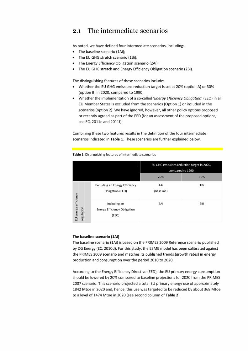
Combining these two features results in the definition of the four intermediate
scenarios indicated in Table 1. These scenarios are further explained below.
Table 1: Distinguishing features of intermediate scenarios
EU GHG emissions reduction target in 2020,
compared to 1990
20% 30%
EU e
ner
gy e
ffic
ien
cy
regu
lati
on
Excluding an Energy Efficiency
Obligation (EEO)
1Ai
(baseline)
1Bi
Including an
Energy Efficiency Obligation
(EEO)
2Ai 2Bi
The baseline scenario (1Ai)
The baseline scenario (1Ai) is based on the PRIMES 2009 Reference scenario published
by DG Energy (EC, 2010d). For this study, the E3ME model has been calibrated against
the PRIMES 2009 scenario and matches its published trends (growth rates) in energy
production and consumption over the period 2010 to 2020.
According to the Energy Efficiency Directive (EED), the EU primary energy consumption
should be lowered by 20% compared to baseline projections for 2020 from the PRIMES
2007 scenario. This scenario projected a total EU primary energy use of approximately
1842 Mtoe in 2020 and, hence, this use was targeted to be reduced by about 368 Mtoe
to a level of 1474 Mtoe in 2020 (see second column of Table 2).
ECN-E--13-033 Methodology 15
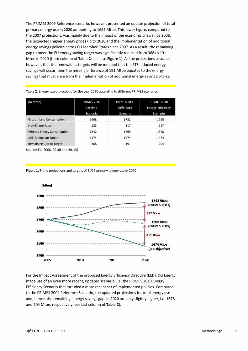
The PRIMES 2009 Reference scenario, however, presented an update projection of total
primary energy use in 2020 amounting to 1665 Mtoe. This lower figure, compared to
the 2007 projections, was mainly due to the impact of the economic crisis since 2008,
the (expected) higher energy prices up to 2020 and the implementation of additional
energy savings policies across EU Member States since 2007. As a result, the remaining
gap to meet the EU energy saving target was significantly reduced from 368 to 191
Mtoe in 2020 (third column of Table 2; see also Figure 1). As the projections assume,
however, that the renewables targets will be met and that the ETS induced energy
savings will occur, then the missing difference of 191 Mtoe equates to the energy
savings that must arise from the implementation of additional energy saving policies.
Table 2: Energy use projections for the year 2020 according to different PRIMES scenarios
[in Mtoe] PRIMES 2007
Baseline
Scenario
PRIMES 2009
Reference
Scenario
PRIMES 2010
Energy Efficiency
Scenario
Gross Inland Consumption 1968 1782 1795
Non-Energy Uses 125 117 117
Primary Energy Consumption 1842 1665 1678
20% Reduction Target 1474 1474 1474
Remaining Gap to Target 368 191 204
Source: EC (2008, 2010d and 2011b)
Figure 1: Trend projections and targets of EU27 primary energy use in 2020
For the Impact Assessment of the proposed Energy Efficiency Directive (EED), DG Energy
made use of an even more recent, updated scenario, i.e. the PRIMES 2010 Energy
Efficiency Scenario that included a more recent set of implemented policies. Compared
to the PRIMES 2009 Reference Scenario, the updated projections for total energy use
and, hence, the remaining ‘energy savings gap’ in 2020 are only slightly higher, i.e. 1678
and 204 Mtoe, respectively (see last column of Table 2).

However, as the PRIMES 2010 Energy Efficiency Scenario has not been made publicly
available for use in this project, we have used the PRIMES 2009 Reference Scenario as
the basis for constructing our baseline scenario (1Ai). The major policy features of this
baseline scenario include:8
It meets the 20% GHG emissions reduction target for the EU27 in 2020;
It meets the 20% renewable energy target for the EU27 in 2020;
It does not include an Energy Efficiency Obligation or any other additional policy
measure proposed by the EED;
It fails to meet the primary energy consumption target proposed by the EED by
about 191 Mtoe in 2020, i.e. more than half of the original target based on the
PRIMES 2007 scenario.
The EU GHG stretch scenario (1Bi)
Scenario 1Bi builds on the baseline scenario 1Ai. The distinguishing feature of scenario
1Bi is that the EU GHG emissions reduction target is enhanced from 20 to 30% in 2020.
In order to reach this target, the EU ETS cap is reduced more or less proportionally by
34% below 2005 ETS emission levels, compared to -21% for the ETS cap in scenario 1Ai
(following EC, 2010a). Given the ambition of this scenario, extra CDM credits are
introduced in the ETS carbon market to account for half of the additional reduction in
ETS emissions. It is important to note, however, that all other policies remain as in the
PRIMES 2009 reference case. It is also left open whether and how the more ambitious
GHG target will be reached in the non-ETS sectors. Therefore, compared to the
baseline, the main difference of scenario 1Bi is that the ETS cap is significantly reduced
(including additional CDM credits), resulting in a proportionally large increase of the ETS
carbon price.
The Energy Efficiency Obligation scenario (2Ai)
Scenario 2Ai also builds on the baseline scenario 1Ai, but this time the distinguishing
feature is that an Energy Efficiency Obligation (EEO) for energy suppliers or distributors
to the sectors Households and Tertiary is introduced in all EU27 Member States. The
EEO obliges MSs to require energy suppliers or distributors to realise savings each year
in all end-use sectors at an amount of 1.5% per annum of their deliveries to customers
or to introduce other policies which will have an equivalent effect. This target includes
the energy savings effects of other, already existing measures which continue to have
an impact in the 2014 to 2020 period and, hence, that the additional impact of the EEO
is likely be less than 1.5% per annum and will vary across EU Member States, depending
on the rate of the energy savings effects of these existing measures. We also make the
assumption that energy suppliers or distributors in each MS contribute 1.0% towards
the 1.5% per annum objective, and that there can be no trading of energy savings
between energy suppliers or distributors in different Member States. In addition, we
assume that the EEO is introduced in January 2014.
The EU GHG stretch and Energy Efficiency Obligation scenario (2Bi)
Scenario 2Bi is a mixture of the scenarios 1Bi and 2Ai in the sense that it is characterised
by both an EU GHG emissions reduction target of 30% in 2020, similar to scenario 1Bi –
with similar implications for the ETS cap and CDM offsets – and the implementation of
an Energy Efficiency Obligation identical to the EEO in scenario 2Ai.
xxxxxxxxxxxxssssssssxxxxxxxxxxxxxx
8 See Appendix A for a more detailed overview of the policies included in the PRIMES 2009 Reference scenario.

ECN-E--13-033 Methodology 17
2.2 Energy saving potentials, investment needs
and public funding
For each of the intermediate scenarios outlined above, the following input variables
have been estimated at both the EU27 level and the individual Member State level:
The currently remaining energy savings potentials up to 2020 for the three target
sectors of this study (Households, Industry and Tertiary);
The (private) investment needs to achieve these potentials;
The public funding or support assumed to be needed in order to induce these
(private) investments.
The methodology to achieve these input variables is explained briefly below, while
more extensive explanations are provided in Appendix B and Appendix C.
Energy saving potentials
The estimation of the energy savings potentials for the present study builds on the so-
called ‘Fraunhofer study’ for the European Commission (EC) on the energy savings
potentials in EU Member States (Eichhammer et al., 2009). The Fraunhofer study
provides estimates of energy savings potentials for the period 2005-2020 for three
types or cases of potentials, i.e. the so-called Low Policy Intensity (LPI) case, the High
Policy Intensity (HPI) case and the Technical Potentials case. These potentials are
detailed for end-use sectors, for fuel and electricity use, and for different applications.
In addition, we have used the more recent ‘Ecofys study’ for the European Climate
Foundation (ECF) on “Energy Savings 2020: How to triple the impact of energy savings
policies in Europe” (Wesselink et al., 2010) and the Regulatory Assistance Project (RAP)
study on “The upfront investments required to double energy savings in the European
Union in 2020” (Wesselink et al., 2011). In the Ecofys study (Wesselink et al., 2010),
which is based on the Fraunhofer study, potentials have been defined with regard to
the HPI case most of the time, but sometimes resemble the Technical Potentials case.
The Ecofys figures are not as detailed as those provided by the Fraunhofer study. For
this study, it has been assumed that the missing Ecofys figures are generally in line with
those for the HPI case.
The Fraunhofer/Ecofys potentials are defined against the Primes 2007 Baseline scenario
for the period 2005-2020. As explained in Section 2.1, however, an updated Primes
2009 Reference scenario was published in 2009 which includes early impacts of the
economic crisis, the implementation of more recent EU and MS energy savings policies,
and the (expected) higher energy prices up to 2020. Compared to the PRIMES 2007
scenario, this leads to a lower trend for energy consumption up to 2020. As a result,
part of the savings potentials identified by Fraunhofer/Ecofys is already used in the
Primes 2009 scenarios due to the higher energy prices and the extra policy measures.
Therefore, the estimates for the energy savings potentials have been updated, using the
increase in energy-intensity per sector as a proxy for the extra savings.
For the purposes of this study it is assumed that only part of the updated and available
energy savings potentials can actually be realised in the time frame to 2020. For
example, if policy makers use the ETS auction revenues to realize the savings potentials
this is only possible from about 2013 onwards, firstly because the revenues start
streaming in that year and, secondly, because it takes some time to set up measures to
stimulate extra savings. As a result, only part of the energy savings potentials can
actually be realised in scenarios with EE measures such as an EEO. The part not
realisable was estimated per category of potentials, based on saving options not applied
over the past years and lost permanently (e.g., new dwellings built but not in
accordance with the Fraunhofer/Ecofys standards up to 2013) and options for which the
period up to 2020 is too short to realize the potential (e.g. new industrial processes; for
more details, see Appendix C).
Per category of energy savings potentials, an effective starting year was assumed that
defined the part to be realized up to 2020. After this second correction, the remaining
energy savings potentials in the baseline scenario 1Ai equal 40-50% of the original
potentials estimated by Fraunhofer/Ecofys. For the other three intermediate scenarios,
estimates of the updated energy savings potentials are even lower since a part of the
potentials available in the baseline scenario is already realised due to the introduction
of the Energy Efficiency Obligation and/or the increase in the EU GHG mitigation target
from 20 to 30% in 2020 and the resulting increase in the ETS carbon price (for further
details, see Section 3.2 and Appendix B). It is assumed that the latter do not need public
support and nor do existing regulations in the baseline which are yet to be implemented
by 2020. Only additional energy saving potential that is achievable before 2020 and that
needs public support is included in these potential estimates. Beyond 2020 there
remains further energy saving potential but the scope of this study is restricted to a
2020 timeframe
Investment needs
In order to estimate the additional investment needs to achieve the updated energy
savings potentials up to 2020, it must first be specified whether investments are really
needed to realize the potential. For instance, for good housekeeping measures or
behavioural changes no, or few, investments are needed. In the Ecofys study and
underlying Fraunhofer study no good housekeeping savings without investments are
specified. In the Ecofys/Fraunhofer study of 2011, dedicated to investment needs for
reaching the savings target of 20%, it is not mentioned whether part of the savings are
realized without investments (Wesselink et al., 2011). In the present study it has been
assumed that for the sectors Households and Tertiary investments are always needed
to achieve energy savings; for Industry it is assumed that part of the savings (10-20%)
are realised through good housekeeping.
The total investments to realize the updated savings potentials are calculated using an
amount of Euros per Ktoe saved. Average figures per sector were taken from the
Ecofys/Fraunhofer 2011 study, taking the mean value from the range specified. The
figures have been differentiated for different categories of savings potentials, keeping
the average figures in line with those of Fraunhofer/Ecofys (for further details, see
Section 3.2 and Appendix B).
ECN-E--13-033 Methodology 19
Public funding requirements
The Fraunhofer/Ecofys potentials are claimed to be cost-effective, meaning that over
the life time of savings measures the annual energy cost savings compensate for the
investment costs annualised by means of a (social) discount rate. This rate, however, is
often lower that the (market) rate usually applied by private energy users. This
difference in social versus private discount rates – or other barriers to private energy
savings investments – may justify some public funding of these investments (assuming
that no other measures to address these barriers and to stimulate these investments
have already been implemented).
In order to estimate the public funding or support assumed to be necessary to induce
the (private) investments to realise the updated energy savings potentials in the target
sectors up to 2020, a default rate of 20% of gross investments has been assumed. For
some parts of energy savings, however, no or less funding has been assumed, e.g. for
good housekeeping in industry. Therefore, the average subsidy rate may vary across the
target sector analysed (see Section 3.2 and Appendix B for further details).
2.3 The energy efficiency investment scenarios
In addition to the four intermediate scenarios (1Ai, 1Bi, 2Ai and 2Bi), four corresponding
‘Investment Scenarios’ have been defined (labelled 1Av, 1Bv, 2Av and 2Bv, respectively,
where the letter ‘i’ refers to ‘intermediate’ and the letter ‘v’ to ‘investment). The
investment scenarios are characterised by the same policy features as their respective
intermediate scenarios (as outlined in Section 2.1). The only difference between the
respective intermediate and investment scenarios is that for the investment scenarios
we assume that the estimated investments required to achieve the updated energy
savings potentials in the target sectors are realised over the period up to 2020 with the
help of carbon revenues, which provide the 20% public funding requirement to
stimulate these savings. In contrast, in the intermediate scenarios these investments
are not realised. Therefore, the difference in outcomes between the investment
scenarios and the respective intermediate scenarios is solely due to including these
investments in the investments scenarios.
2.4 The additional policy scenarios
Finally, in order to address some specific policy issues, we have defined four ‘Additional
Policy Scenarios’. One of these issues is the question of whether there is a difference in
outcomes between stimulating additional energy savings investments in the ETS versus
the non-ETS sectors – and whether stimulating such investments in ETS sectors makes
sense at all - given the interaction effects of these investments with the fixed ETS cap
and the resulting impact on the ETS carbon price.
Therefore, we have defined two policy scenarios, one in which a fixed amount of public
funding to stimulate additional energy savings investments (€ 10 billion per annum, in

current prices, over the period 2013-2020) is focussed solely on the ETS sectors (called
scenario 1Ae) versus one in which a similar amount of public support is concentrated
only on stimulating such investments in the non-ETS sectors (called scenario 1An). In all
other respects these two scenarios are similar to the baseline scenario 1Ai, so – in terms
of the impact of the investments mentioned – they can not only be compared to each
other but also to the baseline scenario.
Other, related issues which are presently discussed – among others in the European
Parliament – include the potential impact on the ETS carbon price of additional energy
savings measures, including the Energy Efficiency Directive (EED) and the Energy
Efficiency Obligation (EEO) in particular, and notably whether this impact could or
should be compensated by a so-called ‘set aside’ of EU ETS allowances (EUAs) and, if
yes, by how much? Therefore, we have defined two other additional policy scenarios:
Scenario 1As. This scenario is similar to the scenario 1Ae mentioned above, i.e. the
baseline scenario including annually € 10 billion of public funding focussed on
stimulating additional energy savings investments in the ETS sectors. The only
difference in this scenarios is that we have set aside an estimated amount of EUAs
(i.e. actually reducing the ETS cap by a similar amount) in order to neutralise the
potential impact of these investments on the ETS carbon price. By comparing the
results of scenario 1As to those of 1Ai, we are able to analyse the effects of such a
set aside on a variety of socioeconomic and environmental outcomes.
Scenario 2At. This scenario is similar to the Energy Efficiency Obligation scenarios
(2Ai), i.e. the baseline scenario including an EEO, as outlined in Section 2.1. The only
difference in this scenario is that we have set aside an estimated amount of EUAs in
order to neutralise the potential impact of this EEO on the ETS carbon price. By
comparing the results of scenario 2At to those of 2Ai, we are able to analyse the
effects of such a set aside on a variety of socioeconomic and environmental
outcomes.
Table 3 provides a summary overview of the distinguishing features of the scenarios
analysed in the present study.
2.5 The E3ME model
In order to assess the scenarios defined above, we have used the Energy-
Environmental-Economy Model for Europe (E3ME), developed by Cambridge
Econometrics (CE). E3ME is a computer-based model of Europe’s economic and energy
systems and the environment. It was originally developed through the European
Commission’s research framework programmes and is now widely used in Europe for
policy assessment, forecasting and research purposes.

ECN-E--13-033 Methodology 21
Table 3: Summary overview of distinguishing features of scenarios analysed
Scenario
acronym
Main features
EU GHG reduction
target in 2020,
compared to 1990
Energy Efficiency
Obligation in all EU27
Member States by
2014?
Additional energy
savings investments in
target sectors?
Set-aside of EU
ETS allowances?
Intermediate scenarios
1Ai 20% No No No
1Bi 30% No No No
2Ai 20% Yes No No
2Bi 30% Yes No No
Investment scenarios
1Av 20% No Yes No
1Bv 30% No Yes No
2Av 20% Yes Yes No
2Bv 30% Yes Yes No
Additional policy scenarios
1Ae 20% No Yes, but only ETS
related sectors
No
1An 20% No Yes, but only
non-ETS related
sectors
No
1As 20% No Yes, but only ETS
related sectors
Yes
2At 20% Yes Yes, both ETS and non-
ETS related sectors
Yes
The structure of E3ME is based on the system of national accounts, as defined by
ESA95, i.e. the Eurostat System of Accounts 1995 (EC, 1996), with further linkages to
energy demand and environmental emissions. The labour market is also covered in
detail, with estimated sets of equations for labour demand, supply, wages and working
hours. In total there are 33 sets of econometrically estimated equations, also including
the components of GDP (consumption, investment, and international trade), prices,
energy demand and materials demand. Each equation set is disaggregated by country
and by sector.
The version of E3ME used in this project includes a historical database that covers the
period 1970-2009 and the model projects forward annually to 2050 (Chewpreecha and
Pollitt, 2009). The main data sources are Eurostat, DG ECFIN’s AMECO database and the
IEA, supplemented by the OECD’s STAN database and other sources where appropriate.
Gaps in the data are estimated using customised software algorithms.
The other main dimensions in this version of the model are:
29 countries (the EU27 member states plus Norway and Switzerland);
42 economic sectors, including disaggregation of the energy sectors and 16 service
sectors;
43 categories of household expenditure;
19 different users of 12 different fuel types;
14 types of air-borne emission (where data are available) including the six
greenhouse gases monitored under the Kyoto protocol;
13 types of household, including income quintiles and socio-economic groups such
as the unemployed, inactive and retired, plus an urban/rural split.
Typical outputs from the model include GDP and sectoral output, household
expenditure, investment, international trade, inflation, employment and
unemployment, energy demand and CO2 emissions. Each of these is available at
national and EU level, and most are also defined by economic sector.
The econometric specification of E3ME gives the model a strong empirical grounding
and means it is not reliant on the assumptions common to Computable General
Equilibrium (CGE) models, such as perfect competition or rational expectations. E3ME
uses a system of error correction, allowing short-term dynamic (or transition)
outcomes, moving towards a long-term trend. The dynamic specification is important
when considering short and medium-term analysis (e.g. up to 2020) and rebound
effects, which are included as standard in the model’s results.9
Figure 2 illustrates the linkages within the E3ME model with regard to the effects of
energy efficiency investments in Households (upper chart) and Industry covered by the
ETS (lower chart). In order to avoid, however, that these charts become too
complicated they show only the main linkages and effects, notably in the Households
diagram. For instance, this diagram does not specify the effects of EE investments on
electricity use which – similar to the effects of EE investments in the Industry diagram –
would have subsequent impacts on the ETS carbon price.
In summary the key strengths of E3ME lie in three different areas:10
The close integration of the economy, energy systems and the environment, with
two-way linkages between each component;
The detailed sectoral disaggregation in the model’s classifications, allowing for the
analysis of similarly detailed scenarios;
The econometric specification of the model, making it suitable for short and
medium-term assessment, as well as longer-term trends;
This makes E3ME a suitable tool to use for running and assessing the scenarios
described in the previous sections. The results from this exercise are presented and
analysed in the following chapter.
xxxxxxxxxxxxssssssssxxxxxxxxxxxxxx
9 Rebound effects occur where an initial increase in efficiency reduces demand, but this is negated in the long run as greater efficiency lowers the relative cost and increases consumption. See Barker et al. (2009).
10 For further details on the model, see Pollitt (2010) and other information included in the E3ME website: http://www.e3me.com

ECN-E--13-033 Methodology 23
Figure 2: E3ME linkages regarding effects of EE investments in Households (upper chart) and in
Industry covered by the EU ETS (lower chart)

3Major results at EU27 level
This chapter presents and discusses the major results at the EU27 level of the scenarios
outlined in the previous chapter. These results refer in particular to (i) energy use and
savings at the sectoral level, (ii) GHG emissions and the ETS carbon price, (iii) scenario
outcomes of the power sector, and (iv) other socio-economic results such as the effects
of the various scenarios on GDP, employment, incomes and international trade.
The results are mainly presented in summary tables and analysed in some detail, first of
all for the intermediate scenarios (Section 3.1). Subsequently, we present our estimates
of the energy savings potentials up to 2020, the investment needs and the public
support to achieve these potentials (Section 3.2). Next, we analyse our results for the
EE investment scenarios (Section 3.3), and finally for the additional policy scenarios
(Section 3.4).
Unless stated otherwise, all results in this chapter refer to the EU27 level in 2020.
3.1 Intermediate scenarios
The baseline scenario (1Ai)
As noted, our baseline scenario has been calibrated and matched to the PRIMES 2009
Reference scenario. Consequently, our baseline scenario shows similar results with
regard to the projected total primary energy use in 2020 (1665 Mtoe) and the
remaining ‘energy savings gap’ (191 Mtoe), given the overall EU target to reduce total
primary energy use to 1474 Mtoe in 2020 (Table 4). In 2020, our baseline scenario
includes an ETS carbon price of 16.5 €/tCO2, total EU GHG emissions of 4309 MtCO2e, a
power price of 107 €/MWh and an average house-hold power bill of € 678 per annum
(Table 5 and Table 6).

ECN-E--13-033 Major results at EU27 level 25
Table 4: Intermediate scenarios (EU27): Primary energy use and energy savings by sectors in 2020 (in
Mtoe)
1Ai 1Bi 2Ai 2Bi
Industry 181 161 186 165
Households 212 210 195 193
Tertiary 94 93 85 84
Sub-total target sectors 487 464 466 442
Other sectors 1178 1155 1170 1149
Total EU27 1665 1620 1636 1592
Target 2020 1474 1474 1474 1474
Energy savings gap 191 146 162 118
Additional energy savings, compared to baseline scenario 1Ai
Industry 0 20 -5 16
Households 0 2 17 19
Tertiary 0 1 9 10
Sub-total target sectors 0 23 22 45
Other sectors 0 23 8 29
Total EU27 0 45 29 73
The EU GHG stretch scenario (1Bi)
In scenario 1Bi the EU GHG mitigation target is increased to 30% in 2020. As explained
in Section 2.1, this is translated in a proportional reduction of the ETS cap – by 30 % in
2020, compared to 2009 ETS emissions – and an increase in offset credits by half of the
resulting additional ETS emissions reduction, while all other policies are assumed to
remain similar to those of the baseline scenario. As a result, the (endogenous) ETS
carbon price (where the model incorporates carbon price dynamics, particularly vis-à-
vis energy demand and explained in more detail below) increases from 16.5 €/tCO2 in
the baseline to 80.0 €/tCO2 in scenario 1Bi, while CO2 emissions in the ETS decline from
2002 to 1837 MtCO2 and total EU GHG emissions from 4309 to 4121 MtCO2 (Table 5).
It should be stressed that the carbon price of €80/t CO2 does not represent our current
assessment of the cost of meeting the 30% target but is designed to illustrate the
potential of extra investment, described below. More recent and detailed analysis of
ETS prices and revenues, using the E3ME model, suggests that a carbon price in the
range of €40-45/t CO2 would be sufficient to meet the target (Vivid Economics, 2012).
The main reasons for the difference are:
the more recent analysis includes more recent (and more negative) data on
Europe’s economies and energy consumption;
recent data and projections of energy prices are lower than previously, meaning
that any increase in EU ETS price has a larger proportional impact on total energy
costs and therefore also on behavioural response;
the recent analysis also includes additional policies that have been implemented;
EUA’s carried over from Phase II have been included in the recent calculations.
While there clearly remains considerable uncertainty about the outcome for the carbon
price, lower carbon prices in the scenarios with a 30% GHG reduction target would not
alter the main conclusions from this analysis, namely that there are sufficient revenues
for investment in energy efficiency and that the economic impacts will generally be
small.
The additional emission reductions are partly accomplished by extra energy savings, in
particular in the industrial ETS sectors. The higher carbon price raises the energy costs
relatively the most in Industry because the base energy prices are relatively low
compared to other sectors. Therefore, most of the extra savings are found for Industry
(about 20 Mtoe in 2020). For the sectors Households and Tertiary only the electricity
price increases – due to the pass-through of the higher ETS carbon prices – and extra
saving are much lower (about 2 and 1 Mtoe, respectively; see Table 4).
Overall, in scenario 1Bi, the additional energy savings in 2020 amount to 23 Mtoe for
the three target sectors as a whole, while the other sectors contribute to extra energy
savings of 23 Mtoe. Therefore, total energy savings amount to 45 Mtoe, resulting in a
remaining energy savings gap of 146 Mtoe in 2020 (Table 4).
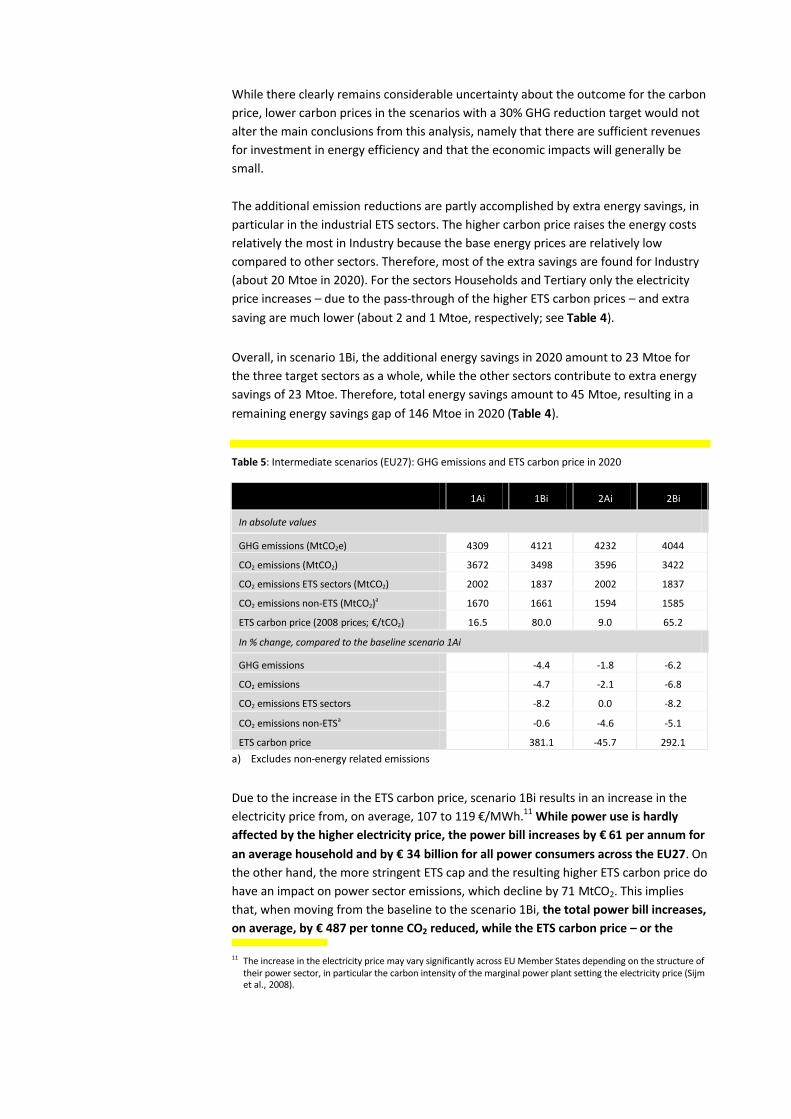
Table 5: Intermediate scenarios (EU27): GHG emissions and ETS carbon price in 2020
1Ai 1Bi 2Ai 2Bi
In absolute values
GHG emissions (MtCO2e) 4309 4121 4232 4044
CO2 emissions (MtCO2) 3672 3498 3596 3422
CO2 emissions ETS sectors (MtCO2) 2002 1837 2002 1837
CO2 emissions non-ETS (MtCO2)a 1670 1661 1594 1585
ETS carbon price (2008 prices; €/tCO2) 16.5 80.0 9.0 65.2
In % change, compared to the baseline scenario 1Ai
GHG emissions -4.4 -1.8 -6.2
CO2 emissions -4.7 -2.1 -6.8
CO2 emissions ETS sectors -8.2 0.0 -8.2
CO2 emissions non-ETSa -0.6 -4.6 -5.1
ETS carbon price 381.1 -45.7 292.1
a) Excludes non-energy related emissions
Due to the increase in the ETS carbon price, scenario 1Bi results in an increase in the
electricity price from, on average, 107 to 119 €/MWh.11 While power use is hardly
affected by the higher electricity price, the power bill increases by € 61 per annum for
an average household and by € 34 billion for all power consumers across the EU27. On
the other hand, the more stringent ETS cap and the resulting higher ETS carbon price do
have an impact on power sector emissions, which decline by 71 MtCO2. This implies
that, when moving from the baseline to the scenario 1Bi, the total power bill increases,
on average, by € 487 per tonne CO2 reduced, while the ETS carbon price – or the xxxxxxxxxxxxssssssssxxxxxxxxxxxxxx
11 The increase in the electricity price may vary significantly across EU Member States depending on the structure of their power sector, in particular the carbon intensity of the marginal power plant setting the electricity price (Sijm et al., 2008).

ECN-E--13-033 Major results at EU27 level 27
marginal costs of CO2 reduction – increases from approximately 17 to 80 €/tCO2 (Table
5 and Table 6). It should be observed, however, that total ETS emissions in this scenario
decline by 165 MtCO2, while auction revenues from the power sector increase from
approximately € 19 billion to € 88 billion in 2020 from which energy end-users may
benefit through higher government expenditures and/or lower taxes.
In scenario 1Bi, as well as in all other following scenarios, almost all of the energy
savings and emission reductions in the so-called ‘other sectors’ originate from the
power sector, with the exception of the ‘B’ scenarios where, in order to meet the lower
ETS cap, a major part of the energy savings also comes from the aviation sector (which
is part of the ETS).
Table 6: Intermediate scenarios (EU27): Power sector results in 2020
1Ai 1Bi 2Ai 2Bi
Power price (in €/MWh)a 107 119 105 116
Total power use (in TWh) 3198 3153 3108 3071
Total power bill (in billion €) 341 376 326 356
Average household power use (in MWh) 4.0 4.0 3.8 3.8
Average household power bill (in €) 678 739 638 689
Power sector emissions (in MtCO2e) 1179 1108 1158 1091
Carbon intensity of power production (in KgCO2/MWh) 369 351 373 355
Changes compared to baseline scenario 1Ai
Change in average household power bill (in €) 61 -40 10
Change in total power bill (in billion €) 34 -16 14
Reduction in power sector emissions (in MtCO2e) 71 21 87
Change in total power bill per tonne CO2e reduced
(in €/tCO2)
487 -754 162
a) Average power price for households and industry. For households only, the average power price is almost 60 per cent higher. Household electricity prices increase comparatively less than other sectors due to the fact that tax makes up a larger proportion of the household electricity price.
The Energy Efficiency Obligation scenario (2Ai)
In scenario 2Ai an Energy Efficiency Obligation is introduced, which refers only to the
consumption of gas and electricity in the sectors Households and Tertiary. As a result,
the energy use in these sectors declines by some 26 Mtoe in 2020. The implementation
of the EEO, however, reduces the ETS carbon price from 16.5 €/tCO2 to 9.0 €/tCO2 in
scenario 2Ai. This is due to the fact that the EEO results in a reduction in power use in
the sectors Households and Tertiary and, hence, to less energy use and less related
emissions in the ETS covered power sector (although less significant than in the
previous scenario, i.e. strengthening the EU ETS cap).
Due to the lower ETS carbon price, however, energy use in Industry becomes cheaper
and, therefore, increases by 5 Mtoe. Overall, due to the EEO, energy use declines, on
balance, by almost 22 Mtoe in the three target sectors, by nearly 8 Mtoe in the other
sectors – i.e. predominantly in the power sector – resulting in a remaining energy
savings gap of about 162 Mtoe up to 2020 (Table 4).

Due to the EEO, CO2 emissions in the non-ETS sector are significantly lower in this
scenario, compared to the baseline as well as to the previous scenario (i.e.
strengthening the EU ETS cap). Compared to the latter scenario, however, emissions in
the EEO scenario are higher in terms of both CO2 emissions in the ETS sector, total EU27
CO emissions and total EU27 GHG emissions (Table 5)
As mentioned above, the EEO leads to a reduction in power use and related emissions.
Note, however, that the decrease in total power sector emissions is slightly less
significant than the decrease in total power use, implying that – due to the lower ETS
carbon price and the resulting switch to more carbon intensive power generation – the
average carbon intensity of power generation in 2020 increases slightly from 369
KgCO2/MWh in the baseline scenario to 373 KgCO2/MWh (Table 6).
In addition to the induced lower power use, the EEO also results in a lower power price
(due to the pass through of a lower ETS carbon price). Overall, in scenario 2Ai, the
power bill is reduced by € 40 per annum for an average household and by € 16 billion
for all power users across the EU27. As power sector emissions decline by 21 MtCO2,
scenario 2Ai leads to a decrease of the EU27 power bill implying on average a benefit
in terms of lower power bills of € 754 per tonne CO2 reduction. Therefore, on the one
hand, the EEO scenario 2Ai results in less energy use and lower energy bills at the EU27
and household levels. On the other hand, however, it results in a 1% increase in the
average carbon intensity of power generation, a halved ETS carbon price and, hence, a
corresponding decrease in ETS auction revenues.
The EU GHG stretch and EEO scenario (2Bi)
As scenario 2Bi combines the distinguishing features of the two previous scenario (i.e.
both a 30% GHG mitigation target and an EEO), it provides a cumulative mix of the
outcomes of these scenarios. Overall, it results in significant energy savings in Industry,
Households and Tertiary totalling about 45 Mtoe for these three target sectors as a
whole. In addition, it leads to substantial energy savings in the other sectors of the EU,
thereby reducing in total the energy savings gap by 73 Mtoe to a remaining target level
of 118 Mtoe in 2020 (Table 4).
In addition it results in a reduction of GHG emissions, including power sector emissions,
by some 6% - relative to the baseline – and an ETS carbon price between the two
‘extremes’ of the two previous scenarios, i.e. about 65 €/tCO2 (again likely to be an
over-estimate given more recent developments). Compared to the baseline, this higher
carbon price results in an increase in the power price by approximately 8%. However, as
power use decreases by some 5%, the power bill is increased by €10 per annum for an
average household and by € 14 billion for all power users across the EU27. (Table 5
and Table 6).
Other socioeconomic outcomes
Table 7 presents some other, socioeconomic outcomes of the baseline scenario (in
absolute terms) and the three other intermediate scenarios (in % change compared to
the baseline). In scenario 1Bi, the tightening of the ETS cap to a 34% reduction
compared to 2005 CO2 emissions levels, as opposed to 21% in the baseline, causes the
EU allowance price to increase almost five-fold to 80 €/tCO2 in 2008 real terms which
has some negative economic consequences. More specifically, the increase in the EU
ECN-E--13-033 Major results at EU27 level 29
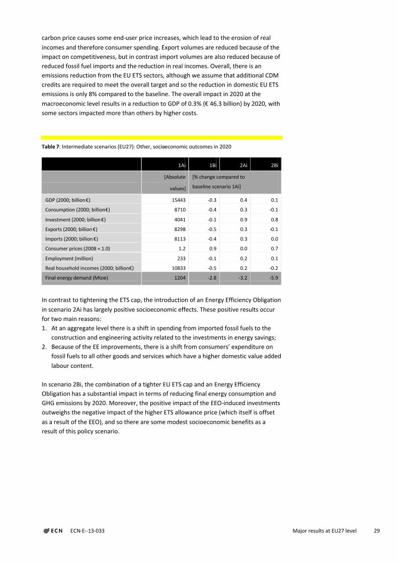
carbon price causes some end-user price increases, which lead to the erosion of real
incomes and therefore consumer spending. Export volumes are reduced because of the
impact on competitiveness, but in contrast import volumes are also reduced because of
reduced fossil fuel imports and the reduction in real incomes. Overall, there is an
emissions reduction from the EU ETS sectors, although we assume that additional CDM
credits are required to meet the overall target and so the reduction in domestic EU ETS
emissions is only 8% compared to the baseline. The overall impact in 2020 at the
macroeconomic level results in a reduction to GDP of 0.3% (€ 46.3 billion) by 2020, with
some sectors impacted more than others by higher costs.
Table 7: Intermediate scenarios (EU27): Other, socio-economic outcomes in 2020
1Ai 1Bi 2Ai 2Bi
[Absolute
values]
[% change compared to
baseline scenario 1Ai]
GDP (2000; billion €) 15443 -0.3 0.4 0.1
Consumption (2000; billion €) 8710 -0.4 0.3 -0.1
Investment (2000; billion €) 4041 -0.1 0.9 0.8
Exports (2000; billion €) 8298 -0.5 0.3 -0.1
Imports (2000; billion €) 8113 -0.4 0.3 0.0
Consumer prices (2008 = 1.0) 1.2 0.9 0.0 0.7
Employment (million) 233 -0.1 0.2 0.1
Real household incomes (2000; billion €) 10833 -0.5 0.2 -0.2
Final energy demand (Mtoe) 1204 -2.8 -3.2 -5.9
In contrast to tightening the ETS cap, the introduction of an Energy Efficiency Obligation
in scenario 2Ai has largely positive socioeconomic effects. These positive results occur
for two main reasons:
1. At an aggregate level there is a shift in spending from imported fossil fuels to the
construction and engineering activity related to the investments in energy savings;
2. Because of the EE improvements, there is a shift from consumers’ expenditure on
fossil fuels to all other goods and services which have a higher domestic value added
labour content.
In scenario 2Bi, the combination of a tighter EU ETS cap and an Energy Efficiency
Obligation has a substantial impact in terms of reducing final energy consumption and
GHG emissions by 2020. Moreover, the positive impact of the EEO-induced investments
outweighs the negative impact of the higher ETS allowance price (which itself is offset
as a result of the EEO), and so there are some modest socioeconomic benefits as a
result of this policy scenario.
3.2 Energy savings potentials, investment needs
and public funding
For each intermediate scenario in 2020, we have estimated remaining energy savings
potentials in the sectors Households, Tertiary and Industry at the EU27 level, as well as
the investment needs and required public funding to realise these potentials (as
outlined briefly in Section 2.2, with further details in Appendix B and Appendix C).
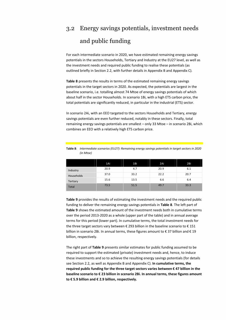
Table 8 presents the results in terms of the estimated remaining energy savings
potentials in the target sectors in 2020. As expected, the potentials are largest in the
baseline scenario, i.e. totalling almost 74 Mtoe of energy savings potentials of which
about half in the sector Households. In scenario 1Bi, with a high ETS carbon price, the
total potentials are significantly reduced, in particular in the industrial (ETS) sector.
In scenario 2Ai, with an EEO targeted to the sectors Households and Tertiary, energy
savings potentials are even further reduced, notably in these sectors. Finally, total
remaining energy savings potentials are smallest – only 33 Mtoe – in scenario 2Bi, which
combines an EEO with a relatively high ETS carbon price.
Table 8: Intermediate scenarios (EU27): Remaining energy savings potentials in target sectors in 2020
(in Mtoe)
1Ai 1Bi 2Ai 2Bi
Industry20.9 4.7 20.9 6.1
Households37.0 33.2 22.2 20.7
Tertiary15.6 13.5 6.6 6.4
Total73.5 51.5 49.7 33.3
Table 9 provides the results of estimating the investment needs and the required public
funding to deliver the remaining energy savings potentials in Table 8. The left part of
Table 9 shows the estimated amount of the investment needs both in cumulative terms
over the period 2013-2020 as a whole (upper part of the table) and in annual average
terms for this period (lower part). In cumulative terms, the total investment needs for
the three target sectors vary between € 293 billion in the baseline scenario to € 151
billion in scenario 2Bi. In annual terms, these figures amount to € 37 billion and € 19
billion, respectively.
The right part of Table 9 presents similar estimates for public funding assumed to be
required to support the estimated (private) investment needs and, hence, to induce
these investments and so to achieve the resulting energy savings potentials (for details
see Section 2.2, as well as Appendix B and Appendix C). In cumulative terms, the
required public funding for the three target sectors varies between € 47 billion in the
baseline scenario to € 23 billion in scenario 2Bi. In annual terms, these figures amount
to € 5.9 billion and € 2.9 billion, respectively.

ECN-E--13-033 Major results at EU27 level 31
Table 9: Intermediate scenarios (EU27): Investment needs to achieve energy savings potentials in
target sectors in 2020 (in billion €)
Investment needs Required public funding
1Ai 1Bi 2Ai 2Bi 1Ai 1Bi 2Ai 2Bi
Cumulative needs over the period 2013-2020
Households180 163 111 104 28.8 26.1 17.7 16.5
Tertiary68 61 33 32 12.5 11.6 6.6 6.4
Industry45 12 45 15 5.9 0.1 5.9 0.4
Total293 236 189 151 47.3 37.9 30.2 23.4
Average annual needs over the period 2013-2020
Households 22.5 20.4 13.9 13.0 3.6 3.3 2.2 2.1
Tertiary 8.5 7.6 4.1 4.0 1.6 1.5 0.8 0.8
Industry 5.6 1.5 5.6 1.9 0.7 0.0 0.7 0.1
Total 36.6 29.5 23.6 18.9 5.9 4.7 3.8 2.9
Finally, Table 10 compares the estimates of the ETS auction revenues in the
intermediate scenarios to the estimates of the public funding requirements to meet the
energy savings potentials in the target sectors up to 2020. ETS auction revenues have
been estimated by multiplying the annual ETS carbon price by the annual amount of EU
allowances (EUAs) that the power sector needs to cover its emissions over the third
trading period, 2013-2020. Hence, it is assumed that:
In all EU27 Member States the power sector has to cover all its emissions by
surrendering EUAs bought at a public auction, thereby abstaining from the fact that
(i) the power sector in Central and Eastern Europe will continue to receive a
significant but declining share of its necessary allowances for free (i.e. 70% in 2013,
declining to zero in 2020), and (ii) the power sector may also buy an eventual
surplus of allowances allocated for free to the industrial sectors on the secondary
EUA market.
In all EU27 Member States the full amount of EUAs destined for the industrial
sectors will continued to be allocated for free up to 2020.
Table 10 shows that over the period 2013-2020 as a whole total ETS auction revenues
at the EU27 level are generally more than sufficient to cover the public support needs
to realise the remaining energy savings potentials in the target sector up to 2020. In
the baseline scenario, for instance, auction revenues are estimated at, on average, € 18
billion per annum and the public funding needs at € 6 billion, resulting in a ‘surplus’ or
balance of ETS auction revenues of € 12 billion per annum. This surplus is substantially
higher in scenario 1Bi (i.e. € 81 billion per annum), predominantly due to the higher ETS
carbon price in this scenario. But even in scenario 2Ai – where the implementation of
the EEO leads to a lower carbon price and, hence, to lower auction revenues – there is
still a significant surplus of these revenues, partly because of the lower remaining
energy savings potentials in the target sectors and, therefore, the lower public funding
needs to realise these potentials.
It should be emphasized that the estimated auction revenues in Table 10 refer to the
intermediate scenarios. Realising additional energy savings in the ETS sectors, however,

reduces the ETS carbon price and, hence, the auction revenues as will be outlined in the
next section when discussing the results of the investment scenarios. In addition, this
section will also make some other qualifications to the estimates of both the auction
revenues and the public support needs presented in Table 10.
Table 10: Intermediate scenarios (EU27): Comparison of ETS auction revenues and public support
needs to meet energy savings potentials in target sectors up to 2020 (in billion €)
ETS auction revenues Public support needs Balance
Cumulative
2013-2020
Annual
average
Cumulative
2013-2020
Annual
average
Cumulative
2013-2020
Annual
average
1Av 144.4 18.1 47.3 5.9 97.1 12.1
1Bv 685.9 85.7 37.9 4.7 648.0 81.0
2Av 114.0 14.3 30.2 3.8 83.8 10.5
2Bv 615.6 76.9 23.4 2.9 592.2 74.0
3.3 Investment scenarios
As explained in Chapter 2, including the estimated amounts of public funding and the
resulting additional energy savings investments in the four intermediate scenarios (1Ai,
1Bi, 2Ai and 2Bi) leads to the respective investment scenarios (1Av, 1Bv, 2Av and 2Bv).
The performance of these investment scenarios is summarised in Table 11 up to Table
16 and is briefly discussed below.
For each investment scenario, Table 11 presents the additional energy savings due to
the extra energy efficiency investments, compared to the respective intermediate
scenarios. For the three target sectors as a whole, these savings vary from 19 Mtoe in
scenario 2Bv to 51 Mtoe in 1Av. Moreover, scenario 2Bv results in additional energy
savings in the other sectors amounting to 24 Mtoe (see bottom part of, Table 11).
In addition, Table 11 shows the combined energy saving effects for each investment
scenario compared to the baseline scenario, i.e. the total energy saving effects of the
extra EE investments and raising the ETS cap/introducing the EEO. For the three
relevant scenarios (1Bv, 2Av and 2Bv), these effects vary from 53 to 64 Mtoe for the
three target sectors as a whole, and from 22 to 37 Mtoe for the other sectors.

ECN-E--13-033 Major results at EU27 level 33
Table 11: Investment scenarios (EU27): Primary energy use and energy savings by sectors in 2020 (in
Mtoe)
1Av 1Bv 2Av 2Bv
Industry 175 170 175 169
Households 177 179 174 174
Tertiary 83 85 81 80
Sub-total target sectors 436 434 430 424
Other sectors 1153 1141 1155 1141
Total EU27 1590 1576 1587 1566
Target 2020 (baseline) 1474 1474 1474 1474
Energy savings gap 116 102 113 92
Additional energy savings, compared to baseline scenario 1Ai
Industry 6 11 6 11
Households 35 33 38 38
Tertiary 11 10 14 14
Sub-total target sectors 51 53 57 64
Other sectors 24 37 22 37
Total EU27 75 89 78 99
Additional energy savings, compared to each respective intermediate scenarioa
Industry 6 -9 10 -4
Households 35 32 21 19
Tertiary 11 8 5 4
Sub-total target sectors 51 31 36 19
Other sectors 24 14 14 8
Total EU27 75 43 49 26
a) That is scenario 1Av to scenario 1Ai, scenario 1Bv to scenario 1Bi, etc.
In order to assess the net effectiveness of the additional EE investments, Table 12
provides a comparison of the estimated energy savings potentials in the four
intermediate scenarios and the realised energy savings in the respective investment
scenarios. The left part of the table provides data on energy savings realised with an
endogenous carbon price, i.e. determined within the model by input variables such as
the level of EE investments. The right part shows similar data with an exogenous carbon
price, i.e. fixed at a level before the additional EE investments are made.
The first or upper part of Table 12 presents data on the energy savings potentials up to
2020 before additional EE investments are made to achieve these potentials. The
second part provides the energy savings realised after the investments have been
implemented. The third part gives the balance or difference between the savings
potentials and the savings realised, while the fourth part expresses the savings realised
as a percentage of the potentials. Subsequently, the table shows the endogenous
carbon price on the left and the exogenous carbon price on the right. The endogenous
price takes into account the effect of EE investment on the carbon price. The exogenous
carbon price is fixed at the level before extra investments are made. Finally, the bottom
line indicates the % change in GDP for each respective scenario.
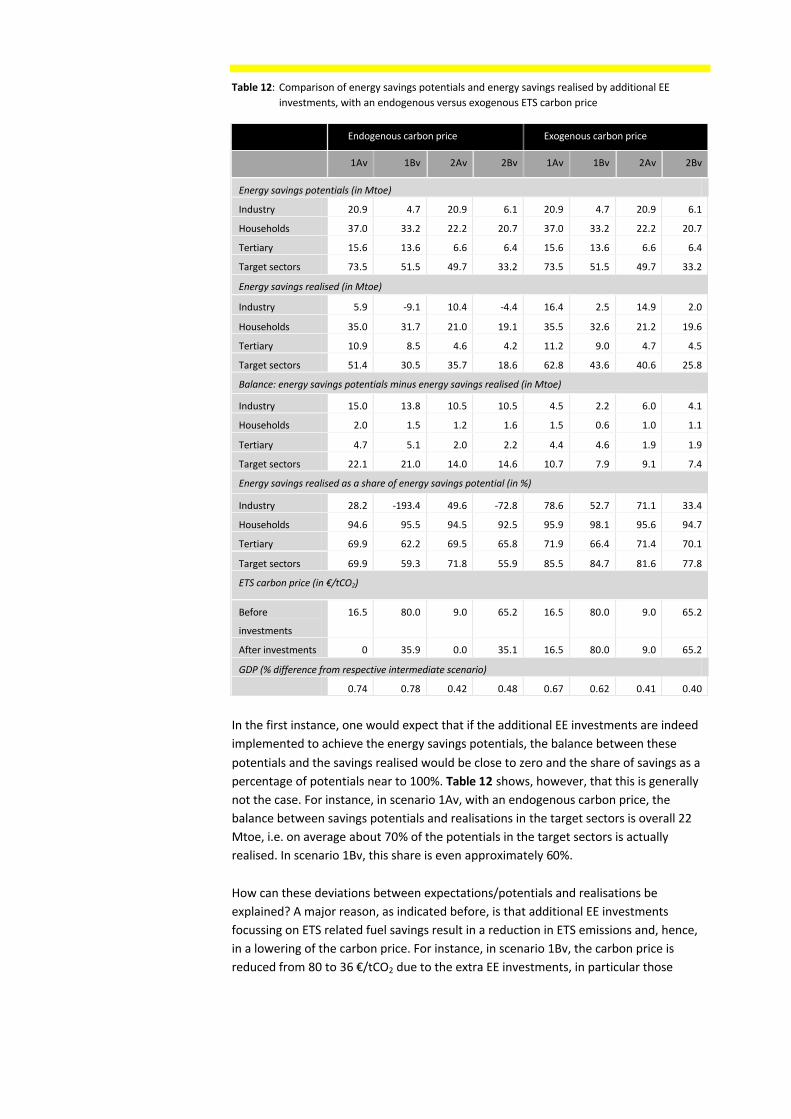
Table 12: Comparison of energy savings potentials and energy savings realised by additional EE
investments, with an endogenous versus exogenous ETS carbon price
Endogenous carbon price Exogenous carbon price
1Av 1Bv 2Av 2Bv 1Av 1Bv 2Av 2Bv
Energy savings potentials (in Mtoe)
Industry 20.9 4.7 20.9 6.1 20.9 4.7 20.9 6.1
Households 37.0 33.2 22.2 20.7 37.0 33.2 22.2 20.7
Tertiary 15.6 13.6 6.6 6.4 15.6 13.6 6.6 6.4
Target sectors 73.5 51.5 49.7 33.2 73.5 51.5 49.7 33.2
Energy savings realised (in Mtoe)
Industry 5.9 -9.1 10.4 -4.4 16.4 2.5 14.9 2.0
Households 35.0 31.7 21.0 19.1 35.5 32.6 21.2 19.6
Tertiary 10.9 8.5 4.6 4.2 11.2 9.0 4.7 4.5
Target sectors 51.4 30.5 35.7 18.6 62.8 43.6 40.6 25.8
Balance: energy savings potentials minus energy savings realised (in Mtoe)
Industry 15.0 13.8 10.5 10.5 4.5 2.2 6.0 4.1
Households 2.0 1.5 1.2 1.6 1.5 0.6 1.0 1.1
Tertiary 4.7 5.1 2.0 2.2 4.4 4.6 1.9 1.9
Target sectors 22.1 21.0 14.0 14.6 10.7 7.9 9.1 7.4
Energy savings realised as a share of energy savings potential (in %)
Industry 28.2 -193.4 49.6 -72.8 78.6 52.7 71.1 33.4
Households 94.6 95.5 94.5 92.5 95.9 98.1 95.6 94.7
Tertiary 69.9 62.2 69.5 65.8 71.9 66.4 71.4 70.1
Target sectors 69.9 59.3 71.8 55.9 85.5 84.7 81.6 77.8
ETS carbon price (in €/tCO2)
Before
investments
16.5 80.0 9.0 65.2 16.5 80.0 9.0 65.2
After investments 0 35.9 0.0 35.1 16.5 80.0 9.0 65.2
GDP (% difference from respective intermediate scenario)
0.74 0.78 0.42 0.48 0.67 0.62 0.41 0.40
In the first instance, one would expect that if the additional EE investments are indeed
implemented to achieve the energy savings potentials, the balance between these
potentials and the savings realised would be close to zero and the share of savings as a
percentage of potentials near to 100%. Table 12 shows, however, that this is generally
not the case. For instance, in scenario 1Av, with an endogenous carbon price, the
balance between savings potentials and realisations in the target sectors is overall 22
Mtoe, i.e. on average about 70% of the potentials in the target sectors is actually
realised. In scenario 1Bv, this share is even approximately 60%.
How can these deviations between expectations/potentials and realisations be
explained? A major reason, as indicated before, is that additional EE investments
focussing on ETS related fuel savings result in a reduction in ETS emissions and, hence,
in a lowering of the carbon price. For instance, in scenario 1Bv, the carbon price is
reduced from 80 to 36 €/tCO2 due to the extra EE investments, in particular those
ECN-E--13-033 Major results at EU27 level 35
investments resulting in a reduction of direct energy use and related emissions in the
power and industrial ETS sectors.
Due to the lower carbon price and, hence, a pass-through of lower carbon costs to the
electricity price, energy use in ETS sectors and electricity consumption by end-users
actually becomes cheaper and, therefore, energy demand increases. This increase in
energy use partly nullifies the initial energy savings due to the extra EE investments. In
scenario 1Bv, energy use in Industry even increases on balance by 69.1 Mtoe,
predominantly due to the substantial fall in the carbon price before and after the
additional EE investments.
The impact of the induced lower carbon price can be illustrated by fixing the carbon
price exogenously at the level before the extra investments are made (see right part of
Table 12). For instance, in scenario 1Bv, by fixing the carbon price at a level of 80
€/tCO2, energy savings in Households increase from 32 to 33 Mtoe, while in Industry
energy use shifts from an increase of 9.1 Mtoe to a decrease of 2.5 Mtoe. Overall, by
fixing the carbon price, the balance between energy savings potentials and realisations
in scenario 1Bv declines from 21 to 8 Mtoe for the three target sectors as a whole, while
the rate of realisations as a share of potentials increases from 59% to 85%. More
generally, across the four scenarios, Table 12 shows that this rate increases from
some 60-70% in case of an endogenous carbon price to about 75-85% in case of an
exogenous carbon price.
Another reason why the actually realised energy savings are, on balance, lower than the
EE investment related potentials is that the extra EE investments result in a higher GDP
and a lower energy bill, and some of these savings are spent on other, energy-using
activities (‘rebound effects’). For instance, the bottom line of Table 12 shows that GDP
is about 0.5-0.8% higher in the investment scenarios, compared to the respective
intermediate scenarios.12 As total primary energy use in the target sectors amount to
almost 500 Mtoe in 2020, this implies that the impact of a higher GDP amounts to some
2-4 Mtoe, assuming a linear relationship between GDP and energy use in the target
sectors (see also Table 14 below, which illustrates the impact of additional EE
investments on lowering electricity bills).
Table 13 provides the impact of the investment scenarios on GHG emissions in 2020.
Compared to the respective intermediate scenarios, this impact ranges from 0.0% for
CO2 emissions of the ETS sectors in scenarios 1Bv and 2Bv to -6.6% for CO2 emissions of
the non-ETS sectors in scenarios 1Av. It should be noted, however, that the impact of
the extra EE investments on particularly the CO2 emissions in the ETS sectors has been
significantly reduced in scenarios 1Av and 2Av – and even nullified in scenarios 1Bv and
2Bv – due to the existence of a fixed ETS cap and the resulting decrease in the ETS
carbon price. Compared to the respective intermediate scenarios, the decrease of the
ETS carbon price due to the extra EE investments amounts to 55% and 46% in scenarios
1Bv and 2Bv, respectively, and even 100% in scenarios 1Av and 2Av. Therefore,
additional EE investment which reduces ETS related emissions has a decreasing
impact on the ETS carbon price that, in turn, partly or even fully nullifies the impact
on total ETS emissions but also, as noted above, on related energy use.
xxxxxxxxxxxxssssssssxxxxxxxxxxxxxx
12 Note that the increase in GDP is generally higher under an endogenous carbon price, i.e. when the carbon price is lower due to the extra EE investments.

Table 13: Investment scenarios (EU27): GHG emissions and ETS carbon price in 2020
1Av 1Bv 2Av 2Bv
In absolute values
GHG emissions (MtCO2e) 4096 4008 4088 3977
CO2 emissions (MtCO2) 3489 3410 3471 3370
CO2 emissions ETS sectors (MtCO2) 1929 1837 1941 1837
CO2 emissions non-ETS (MtCO2)a 1560 1572 1530 1533
ETS carbon price (2008; €/tCO2) 0.0 35.9 0.0 35.1
In % change, compared to the baseline scenario 1Ai
GHG emissions -4.9 -7.0 -5.1 -7.7
CO2 emissions -5.0 -7.1 -5.5 -8.2
CO2 emissions ETS sectors -3.6 -8.2 -3.0 -8.2
CO2 emissions non-ETSa -6.6 -5.8 -8.4 -8.2
ETS carbon price -100.0 116.0 -100.0 111.0
In % change, compared to each respective intermediate scenariob
GHG emissions -4.9 -2.8 -3.4 -1.7
CO2 emissions -5.0 -2.5 -3.5 -1.5
CO2 emissions ETS sectors -3.6 0.0 -3.0 0.0
CO2 emissions non-ETSa -6.6 -5.3 -4.0 -3.3
ETS carbon price -100.0 -55.1 -100.0 -46.2
a) Excludes non-energy related emissions. b) That is scenario 1Av to scenario 1Ai, scenario 1Bv to scenario 1Bi, etc.
Table 14 presents the results of the investment scenarios for the power sector in 2020.
Compared to the respective intermediate scenarios, the extra EE investments lead to, in
general, lower power use and lower power prices. As a result, the power bill in 2020 is
significantly reduced, ranging at the EU27 level from € 28 billion in scenario 2Av to € 54
billion in 1Bv and, at the average household level, from € 68 in 2Av to € 140 in 1Bv.
Moreover, due to the extra EE investments and the resulting lower power use, GHG
emissions in the power sector are reduced by 31 MtCO2e in scenario 2Bv to 92 MtCO2e
in 1Av. This implies that the EU27 power bill decreased by, on average, € 505 per tonne
CO2 reduction in scenario 1Av and by € 1125 per tonne in 2Bv (see bottom part of Table
14).

ECN-E--13-033 Major results at EU27 level 37
Table 14: Investment scenarios (EU27): Power sector results in 2020
1Av 1Bv 2Av 2Bv
Power price (in €/MWh)a 101 108 102 108
Total power use (in TWh) 2916 2987 2921 2967
Total power bill (in billion €) 295 322 298 321
Average household power use (in MWh) 3.5 3.5 3.5 3.5
Average household power bill (in €) 563 599 570 602
Power sector emissions (in MtCO2e) 1087 1060 1099 1061
Carbon intensity of power production (in KgCO2/MWh) 373 355 376 357
Changes compared to baseline scenario 1Ai
Change in average household power bill (in €) -115 -79 -108 -76
Change in total power bill (in billion €) -46 -20 -44 -20
Reduction in power sector emissions (in MtCO2e) 92 119 80 118
Change in total power bill per tonne CO2e reduced
(in €/tCO2)
-505 -165 -549 -171
Changes compared to each respective intermediate scenariob
Change in average household power bill (in €) -115 -140 -68 -86
Change in total power bill (in billion €) -46 -54 -28 -34
Reduction in power sector emissions (in MtCO2e) 92 48 59 31
Change in total power bill per tonne CO2e reduced
(in €/tCO2)
-505 -
1125
-477 -
1125
a) Average power price for households and industry. For households only, the average power price is almost 60 per cent higher.
b) That is scenario 1Av to scenario 1Ai, scenario 1Bv to scenario 1Bi, etc.
Hence, from a power bill perspective, reducing power sector emissions through
stimulating EE investments seems to be a more attractive strategy than by means of
reducing the ETS cap and, thereby, increasing the ETS carbon price. As noted, however,
promoting EE investments that reduce ETS/power sector related emissions has a
decreasing impact on the ETS carbon price that, in turn, nullifies the impact on total ETS
emissions but also reduces the impact on related energy use. That is, as long as the ETS
cap is fixed – and the ETS carbon price is higher than zero – such investments result in
shifting GHG emissions (and related energy use) across ETS sectors rather than reducing
overall ETS emissions.
Therefore, a more useful approach in the long run might be a mixed package of both
increasing the ETS carbon price (by lowering the ETS cap) and using part of the ETS
auction revenues to stimulate investments in energy savings, including electricity
savings. This mitigates the effects of a tighter ETS cap on the ETS carbon price and, both
directly and indirectly, on the household power bill. This is actually the approach
implemented in scenario 1Bv, compared to the baseline scenario 1Ai.
More specifically, these model results suggest that reducing the ETS cap only (i.e.
scenario 1Bi) increases the ETS carbon price from 17 €/tCO2 to 80 €/tCO2, the average
power price from 107 €/MWh to 119 €/MWh, the average household power bill from €
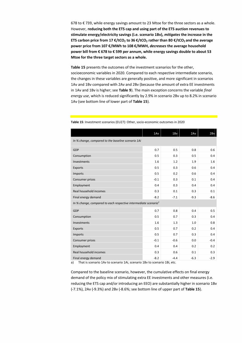
678 to € 739, while energy savings amount to 23 Mtoe for the three sectors as a whole.
However, reducing both the ETS cap and using part of the ETS auction revenues to
stimulate energy/electricity savings (i.e. scenario 1Bv), mitigates the increase in the
ETS carbon price from 17 €/tCO2 to 36 €/tCO2 rather than 80 €/tCO2 and the average
power price from 107 €/MWh to 108 €/MWH, decreases the average household
power bill from € 678 to € 599 per annum, while energy savings double to about 53
Mtoe for the three target sectors as a whole.
Table 15 presents the outcomes of the investment scenarios for the other,
socioeconomic variables in 2020. Compared to each respective intermediate scenario,
the changes in these variables are generally positive, and more significant in scenarios
1Av and 1Bv compared with 2Av and 2Bv (because the amount of extra EE investments
in 1Av and 1Bv is higher; see Table 9). The main exception concerns the variable final
energy use, which is reduced significantly by 2.9% in scenario 2Bv up to 8.2% in scenario
1Av (see bottom line of lower part of Table 15).
Table 15: Investment scenarios (EU27): Other, socio-economic outcomes in 2020
1Av 1Bv 2Av 2Bv
In % change, compared to the baseline scenario 1Ai
GDP 0.7 0.5 0.8 0.6
Consumption 0.5 0.3 0.5 0.4
Investments 1.6 1.2 1.9 1.6
Exports 0.5 0.3 0.6 0.4
Imports 0.5 0.2 0.6 0.4
Consumer prices -0.1 0.3 0.1 0.4
Employment 0.4 0.3 0.4 0.4
Real household incomes 0.3 0.1 0.3 0.1
Final energy demand -8.2 -7.1 -9.3 -8.6
In % change, compared to each respective intermediate scenarioa
GDP 0.7 0.8 0.4 0.5
Consumption 0.5 0.7 0.3 0.4
Investments 1.6 1.3 1.0 0.8
Exports 0.5 0.7 0.2 0.4
Imports 0.5 0.7 0.3 0.4
Consumer prices -0.1 -0.6 0.0 -0.4
Employment 0.4 0.4 0.2 0.2
Real household incomes 0.3 0.6 0.1 0.3
Final energy demand -8.2 -4.4 -6.3 -2.9
a) That is scenario 1Av to scenario 1Ai, scenario 1Bv to scenario 1Bi, etc.
Compared to the baseline scenario, however, the cumulative effects on final energy
demand of the policy mix of stimulating extra EE investments and other measures (i.e.
reducing the ETS cap and/or introducing an EEO) are substantially higher in scenario 1Bv
(-7.1%), 2Av (-9.3%) and 2Bv (-8.6%; see bottom line of upper part of Table 15).
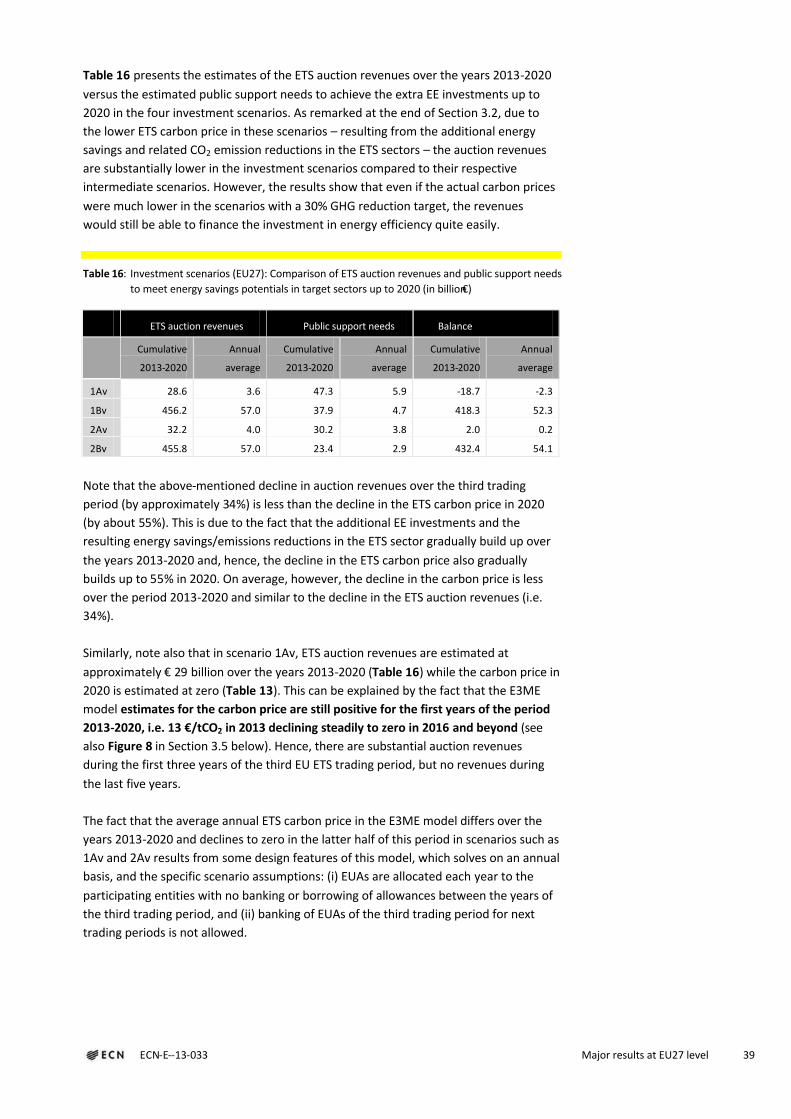
ECN-E--13-033 Major results at EU27 level 39
Table 16 presents the estimates of the ETS auction revenues over the years 2013-2020
versus the estimated public support needs to achieve the extra EE investments up to
2020 in the four investment scenarios. As remarked at the end of Section 3.2, due to
the lower ETS carbon price in these scenarios – resulting from the additional energy
savings and related CO2 emission reductions in the ETS sectors – the auction revenues
are substantially lower in the investment scenarios compared to their respective
intermediate scenarios. However, the results show that even if the actual carbon prices
were much lower in the scenarios with a 30% GHG reduction target, the revenues
would still be able to finance the investment in energy efficiency quite easily.
Table 16: Investment scenarios (EU27): Comparison of ETS auction revenues and public support needs
to meet energy savings potentials in target sectors up to 2020 (in billion €)
ETS auction revenues Public support needs Balance
Cumulative
2013-2020
Annual
average
Cumulative
2013-2020
Annual
average
Cumulative
2013-2020
Annual
average
1Av 28.6 3.6 47.3 5.9 -18.7 -2.3
1Bv 456.2 57.0 37.9 4.7 418.3 52.3
2Av 32.2 4.0 30.2 3.8 2.0 0.2
2Bv 455.8 57.0 23.4 2.9 432.4 54.1
Note that the above-mentioned decline in auction revenues over the third trading
period (by approximately 34%) is less than the decline in the ETS carbon price in 2020
(by about 55%). This is due to the fact that the additional EE investments and the
resulting energy savings/emissions reductions in the ETS sector gradually build up over
the years 2013-2020 and, hence, the decline in the ETS carbon price also gradually
builds up to 55% in 2020. On average, however, the decline in the carbon price is less
over the period 2013-2020 and similar to the decline in the ETS auction revenues (i.e.
34%).
Similarly, note also that in scenario 1Av, ETS auction revenues are estimated at
approximately € 29 billion over the years 2013-2020 (Table 16) while the carbon price in
2020 is estimated at zero (Table 13). This can be explained by the fact that the E3ME
model estimates for the carbon price are still positive for the first years of the period
2013-2020, i.e. 13 €/tCO2 in 2013 declining steadily to zero in 2016 and beyond (see
also Figure 8 in Section 3.5 below). Hence, there are substantial auction revenues
during the first three years of the third EU ETS trading period, but no revenues during
the last five years.
The fact that the average annual ETS carbon price in the E3ME model differs over the
years 2013-2020 and declines to zero in the latter half of this period in scenarios such as
1Av and 2Av results from some design features of this model, which solves on an annual
basis, and the specific scenario assumptions: (i) EUAs are allocated each year to the
participating entities with no banking or borrowing of allowances between the years of
the third trading period, and (ii) banking of EUAs of the third trading period for next
trading periods is not allowed.

Nevertheless, despite the decline in the ETS auction revenues resulting from the extra
EE investments, Table 16 shows that, in principle, these revenues are still adequate to
cover the public funding needs to support these investments in three out of four of
the investment scenarios. The exception is scenario 1Av, in which the auction revenues
are estimated at, on average, € 3.6 billion per annum over the period 2013-220 and the
public EE support needs at € 5.9 billion, resulting in a funding deficit of € 2.3 billion per
annum.
Some qualification, however, can be added to the above-mentioned findings on the
balance between ETS auction revenues and public EE funding needs:
The observations made above assume that the ETS auction revenues will be
available for funding public support of additional energy savings investments. The
EU ETS Directive, however, recommends that 50% of the auction revenues ought to
be spent on climate policy issues, but this share is not binding. Moreover, this
percentage refers to all climate policy spending, both existing and new/additional,
including other climate policy expenditures beyond stimulating EE investments, such
as promoting renewables or other climate friendly technologies, financing climate
adaptation measures, providing climate finance support to non-Annex I countries, or
compensating end-users for ETS induced higher electricity prices. Hence, in practice,
the amount of ETS auction revenues available for supporting additional EE
investments may be substantially less than actually needed. On the other hand, if
deemed either socially desirable or necessary, extra EE investments may also be
supported from other government resources beyond – or rather than – ETS auction
revenues.
In some Member States, such as the Netherlands or the UK, earmarking of ETS
revenues to funding of climate policy measures is not accepted. That is, government
revenues and government expenditures are considered separately and, hence, ETS
revenues become part of total government revenues used to finance government
expenditures, including recycling ETS revenues to firms and households through
lower taxes or social premiums. As indicated above, however, in such countries
extra EE investments may be supported through funding from public revenues in
general rather than from earmarking to specific ETS auction revenues.
Table 16 presents an aggregated picture for the EU27 as a whole. For individual
Member States, however, the balance between ETS auction revenues and public
support needs may look quite differently. For instance, auction revenues may be
relatively low, notably in countries such as France or Sweden which have a relatively
low share of fossil-fuelled power generation. On the other hand, public EE support
needs may be relatively high in some Member States because there is a relatively
large potential of energy savings potentials in the target sectors or because these
savings need a relatively high level of support to be realised.
The estimates of the auction revenues are based on the projection of a certain ETS
carbon price. For instance, in the baseline – which is calibrated to the 2009 PRIMES
scenario – the ETS carbon price is projected to become 17 €/tCO2 in 2020. Due to
the lasting economic crisis, however, the current (2012) ETS price is about 6-8
€/tCO2 while price expectations for the coming years are similarly low. Hence, actual
ETS carbon prices over the years 2013-2020 may be significantly lower than the
model projected carbon prices underlying the estimates of the auction revenues
presented in Table 16.
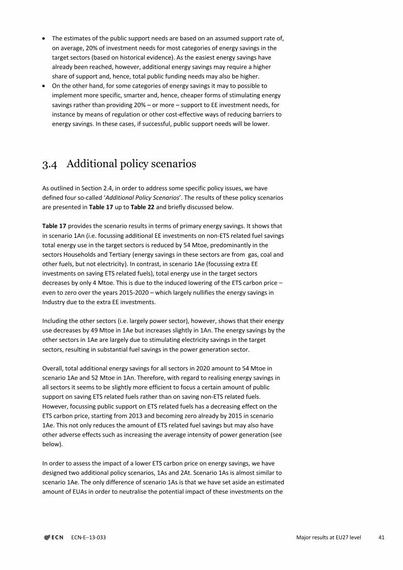
ECN-E--13-033 Major results at EU27 level 41
The estimates of the public support needs are based on an assumed support rate of,
on average, 20% of investment needs for most categories of energy savings in the
target sectors (based on historical evidence). As the easiest energy savings have
already been reached, however, additional energy savings may require a higher
share of support and, hence, total public funding needs may also be higher.
On the other hand, for some categories of energy savings it may to possible to
implement more specific, smarter and, hence, cheaper forms of stimulating energy
savings rather than providing 20% – or more – support to EE investment needs, for
instance by means of regulation or other cost-effective ways of reducing barriers to
energy savings. In these cases, if successful, public support needs will be lower.
3.4 Additional policy scenarios
As outlined in Section 2.4, in order to address some specific policy issues, we have
defined four so-called ‘Additional Policy Scenarios’. The results of these policy scenarios
are presented in Table 17 up to Table 22 and briefly discussed below.
Table 17 provides the scenario results in terms of primary energy savings. It shows that
in scenario 1An (i.e. focussing additional EE investments on non-ETS related fuel savings
total energy use in the target sectors is reduced by 54 Mtoe, predominantly in the
sectors Households and Tertiary (energy savings in these sectors are from gas, coal and
other fuels, but not electricity). In contrast, in scenario 1Ae (focussing extra EE
investments on saving ETS related fuels), total energy use in the target sectors
decreases by only 4 Mtoe. This is due to the induced lowering of the ETS carbon price –
even to zero over the years 2015-2020 – which largely nullifies the energy savings in
Industry due to the extra EE investments.
Including the other sectors (i.e. largely power sector), however, shows that their energy
use decreases by 49 Mtoe in 1Ae but increases slightly in 1An. The energy savings by the
other sectors in 1Ae are largely due to stimulating electricity savings in the target
sectors, resulting in substantial fuel savings in the power generation sector.
Overall, total additional energy savings for all sectors in 2020 amount to 54 Mtoe in
scenario 1Ae and 52 Mtoe in 1An. Therefore, with regard to realising energy savings in
all sectors it seems to be slightly more efficient to focus a certain amount of public
support on saving ETS related fuels rather than on saving non-ETS related fuels.
However, focussing public support on ETS related fuels has a decreasing effect on the
ETS carbon price, starting from 2013 and becoming zero already by 2015 in scenario
1Ae. This not only reduces the amount of ETS related fuel savings but may also have
other adverse effects such as increasing the average intensity of power generation (see
below).
In order to assess the impact of a lower ETS carbon price on energy savings, we have
designed two additional policy scenarios, 1As and 2At. Scenario 1As is almost similar to
scenario 1Ae. The only difference of scenario 1As is that we have set aside an estimated
amount of EUAs in order to neutralise the potential impact of these investments on the
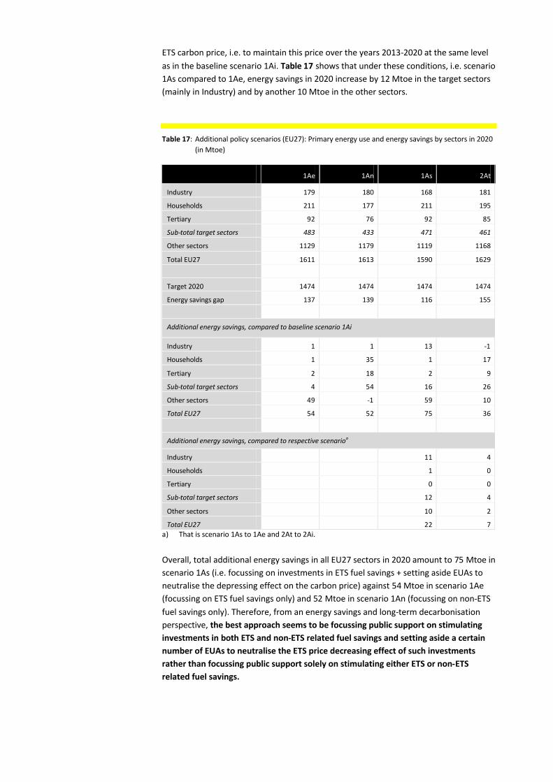
ETS carbon price, i.e. to maintain this price over the years 2013-2020 at the same level
as in the baseline scenario 1Ai. Table 17 shows that under these conditions, i.e. scenario
1As compared to 1Ae, energy savings in 2020 increase by 12 Mtoe in the target sectors
(mainly in Industry) and by another 10 Mtoe in the other sectors.
Table 17: Additional policy scenarios (EU27): Primary energy use and energy savings by sectors in 2020
(in Mtoe)
1Ae 1An 1As 2At
Industry 179 180 168 181
Households 211 177 211 195
Tertiary 92 76 92 85
Sub-total target sectors 483 433 471 461
Other sectors 1129 1179 1119 1168
Total EU27 1611 1613 1590 1629
Target 2020 1474 1474 1474 1474
Energy savings gap 137 139 116 155
Additional energy savings, compared to baseline scenario 1Ai
Industry 1 1 13 -1
Households 1 35 1 17
Tertiary 2 18 2 9
Sub-total target sectors 4 54 16 26
Other sectors 49 -1 59 10
Total EU27 54 52 75 36
Additional energy savings, compared to respective scenarioa
Industry 11 4
Households 1 0
Tertiary 0 0
Sub-total target sectors 12 4
Other sectors 10 2
Total EU27 22 7
a) That is scenario 1As to 1Ae and 2At to 2Ai.
Overall, total additional energy savings in all EU27 sectors in 2020 amount to 75 Mtoe in
scenario 1As (i.e. focussing on investments in ETS fuel savings + setting aside EUAs to
neutralise the depressing effect on the carbon price) against 54 Mtoe in scenario 1Ae
(focussing on ETS fuel savings only) and 52 Mtoe in scenario 1An (focussing on non-ETS
fuel savings only). Therefore, from an energy savings and long-term decarbonisation
perspective, the best approach seems to be focussing public support on stimulating
investments in both ETS and non-ETS related fuel savings and setting aside a certain
number of EUAs to neutralise the ETS price decreasing effect of such investments
rather than focussing public support solely on stimulating either ETS or non-ETS
related fuel savings.
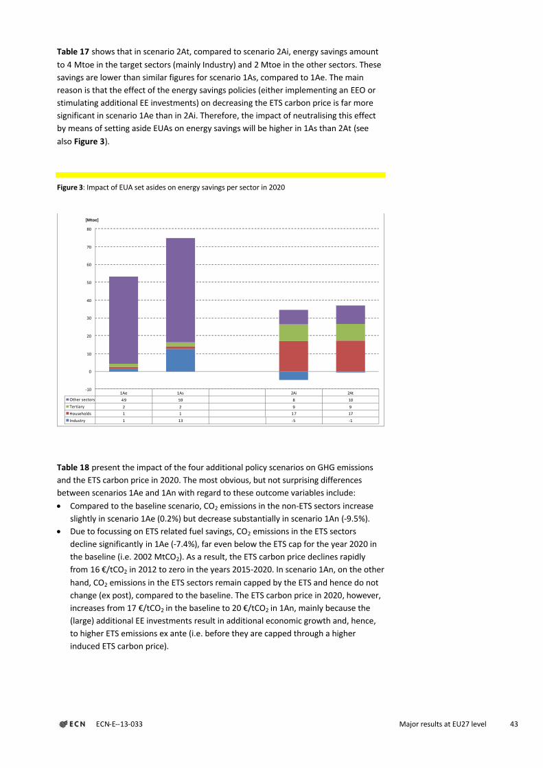
ECN-E--13-033 Major results at EU27 level 43
Table 17 shows that in scenario 2At, compared to scenario 2Ai, energy savings amount
to 4 Mtoe in the target sectors (mainly Industry) and 2 Mtoe in the other sectors. These
savings are lower than similar figures for scenario 1As, compared to 1Ae. The main
reason is that the effect of the energy savings policies (either implementing an EEO or
stimulating additional EE investments) on decreasing the ETS carbon price is far more
significant in scenario 1Ae than in 2Ai. Therefore, the impact of neutralising this effect
by means of setting aside EUAs on energy savings will be higher in 1As than 2At (see
also Figure 3).
Figure 3: Impact of EUA set asides on energy savings per sector in 2020
Table 18 present the impact of the four additional policy scenarios on GHG emissions
and the ETS carbon price in 2020. The most obvious, but not surprising differences
between scenarios 1Ae and 1An with regard to these outcome variables include:
Compared to the baseline scenario, CO2 emissions in the non-ETS sectors increase
slightly in scenario 1Ae (0.2%) but decrease substantially in scenario 1An (-9.5%).
Due to focussing on ETS related fuel savings, CO2 emissions in the ETS sectors
decline significantly in 1Ae (-7.4%), far even below the ETS cap for the year 2020 in
the baseline (i.e. 2002 MtCO2). As a result, the ETS carbon price declines rapidly
from 16 €/tCO2 in 2012 to zero in the years 2015-2020. In scenario 1An, on the other
hand, CO2 emissions in the ETS sectors remain capped by the ETS and hence do not
change (ex post), compared to the baseline. The ETS carbon price in 2020, however,
increases from 17 €/tCO2 in the baseline to 20 €/tCO2 in 1An, mainly because the
(large) additional EE investments result in additional economic growth and, hence,
to higher ETS emissions ex ante (i.e. before they are capped through a higher
induced ETS carbon price).
1Ae 1As 2Ai 2At
Other sectors 49 59 8 10
Tertiary 2 2 9 9
Households 1 1 17 17
Industry 1 13 -5 -1
-10
0
10
20
30
40
50
60
70
80
[Mtoe]

Table 18: Additional policy scenarios (EU27): GHG emissions and ETS carbon price in 2020
1Ae 1An 1As 2At
In absolute values
GHG emissions (MtCO2e) 4154 4150 4086 4209
CO2 emissions (MtCO2) 3528 3513 3461 3574
CO2 emissions ETS sectors (MtCO2) 1854 2002 1790 1982
CO2 emissions non-ETS (MtCO2)a 1674 1511 1671 1593
ETS carbon price (2008; €/tCO2) 0.0 20.0 16.5 16.5
In % change (compared to the baseline scenario 1Ai)
GHG emissions -3.6 -3.7 -5.2 -2.3
CO2 emissions -3.9 -4.3 -5.7 -2.7
CO2 emissions ETS sectors -7.4 0.0 -10.6 -1.0
CO2 emissions non-ETSa 0.2 -9.5 0.1 -4.6
ETS carbon price -100.0 21.2 -0.0 -0.0
In % change, compared to respective scenariob
GHG emissions -1.6 -0.5
CO2 emissions -1.9 -0.6
CO2 emissions ETS sectors -3.4 -1.0
CO2 emissions non-ETSa -0.2 -0.1
ETS carbon price n.a. 83.3.
a) Excludes non-energy related emissions.b) That is scenario 1As to 1Ae and 2At to 2Ai.
In order to neutralise the impact of the additional investments in saving ETS related
fuels on the carbon price (in scenario 1Ae), we have estimated the amount of EUAs that
need to be set aside (resulting in scenario 1As). For comparable reasons, we have
estimated a similar set aside to neutralise the impact of implementing an EEO in
scenario 2Ai, resulting in scenario 2At.
Table 19 shows the estimated amounts of set asides over the years 2013-2020. In
scenario 1As, the set aside amounts to 34 MtCO2 in 2013 and increases steadily to 240
MtCO2 in 2020. Over the period 2013-2020 as a whole, the set aside amount to 1074
MtCO2, i.e. on average 134 MtCO2 per annum or 6.3% of the average ETS cap in this
period. For scenario 2At, the estimated amounts of set asides are significantly lower, i.e.
on average 41 MtCO2 per annum or 1.9% of the average cap over the years 2013-2020.
Table 19: Additional policy scenarios: Estimates of EUA set asides
Total 2013-2020
(MtCO2)
Annual average
(MtCO2)
As % of average EU ETS
cap 2013-2020
1As 1074 134 6.3
2At 328 41 1.9
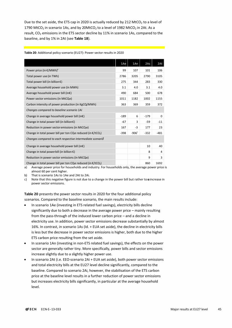
ECN-E--13-033 Major results at EU27 level 45
Due to the set aside, the ETS cap in 2020 is actually reduced by 212 MtCO2 to a level of
1790 MtCO2 in scenario 1As, and by 20MtCO2 to a level of 1982 MtCO2 in 2At. As a
result, CO2 emissions in the ETS sector decline by 11% in scenario 1As, compared to the
baseline, and by 1% in 2At (see Table 18).
Table 20: Additional policy scenario (EU27): Power sector results in 2020
1Ae 1An 2As 2At
Power price (in €/MWh)a 99 107 101 106
Total power use (in TWh) 2786 3205 2790 3105
Total power bill (in billion €) 275 344 283 330
Average household power use (in MWh) 3.1 4.0 3.1 4.0
Average household power bill (in €) 490 684 500 678
Power sector emissions (in MtCO2e) 1011 1182 1002 1155
Carbon intensity of power production (in KgCO2/MWh) 363 369 359 372
Changes compared to baseline scenario 1Ai
Change in average household power bill (in €) -189 6 -179 0
Change in total power bill (in billion €) -67 3 -59 -11
Reduction in power sector emissions (in MtCO2e) 167 -3 177 23
Change in total power bill per ton CO2e reduced (in €/tCO2) -398 -906c -332 -481
Changes compared to each respective intermediate scenariob
Change in average household power bill (in €) 10 40
Change in total power bill (in billion €) 8 4
Reduction in power sector emissions (in MtCO2e) 9 3
Change in total power bill per ton CO2e reduced (in €/tCO2) 860 1692
a) Average power price for households and industry. For households only, the average power price is almost 60 per cent higher.
b) That is scenario 1As to 1Ae and 2At to 2Ai.c) Note that this negative figure is not due to a change in the power bill but rather to an increase in
power sector emissions.
Table 20 presents the power sector results in 2020 for the four additional policy
scenarios. Compared to the baseline scenario, the main results include:
In scenario 1Ae (investing in ETS related fuel savings), electricity bills decline
significantly due to both a decrease in the average power price – mainly resulting
from the pass-through of the induced lower carbon price – and a decline in
electricity use. In addition, power sector emissions decrease substantially by almost
16%. In contrast, in scenario 1As (Id. + EUA set aside), the decline in electricity bills
is less but the decrease in power sector emissions is higher, both due to the higher
ETS carbon price resulting from the set aside.
In scenario 1An (investing in non-ETS related fuel savings), the effects on the power
sector are generally rather tiny. More specifically, power bills and sector emissions
increase slightly due to a slightly higher power use.
In scenario 2At (i.e. EEO-scenario 2Ai + EUA set aside), both power sector emissions
and total electricity bills at the EU27 level decline significantly, compared to the
baseline. Compared to scenario 2Ai, however, the stabilisation of the ETS carbon
price at the baseline level results in a further reduction of power sector emissions
but increases electricity bills significantly, in particular at the average household
level.
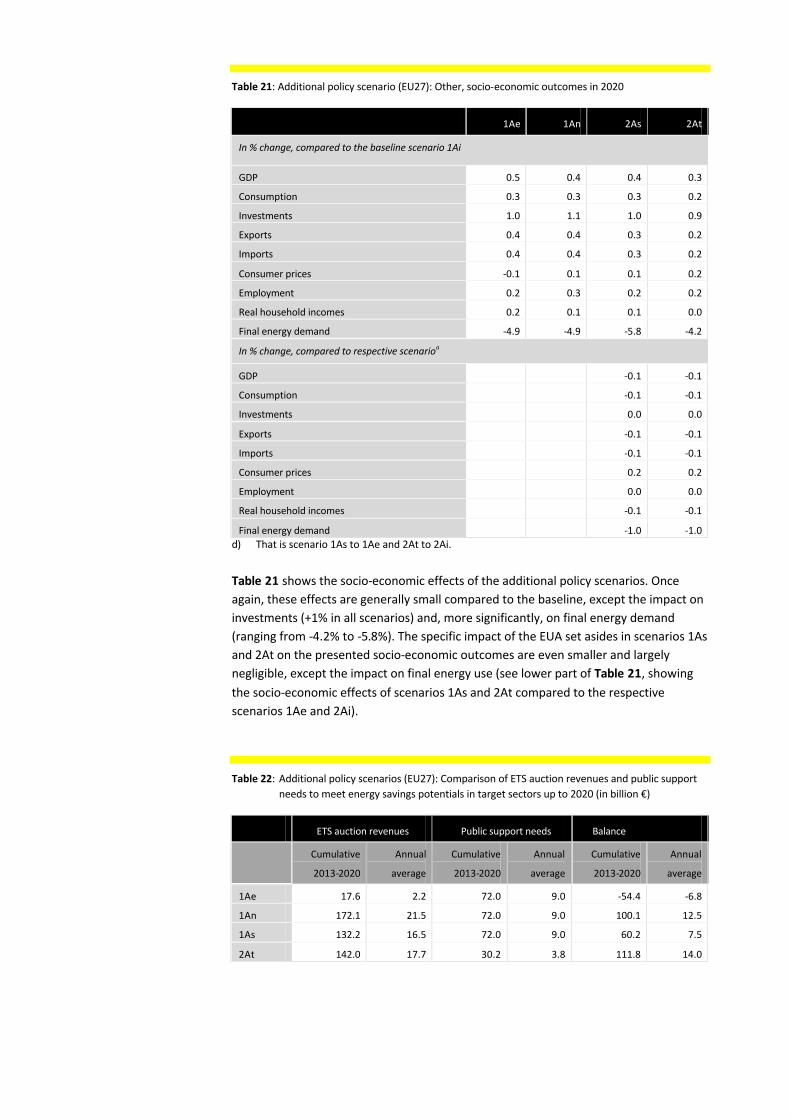
Table 21: Additional policy scenario (EU27): Other, socio-economic outcomes in 2020
1Ae 1An 2As 2At
In % change, compared to the baseline scenario 1Ai
GDP 0.5 0.4 0.4 0.3
Consumption 0.3 0.3 0.3 0.2
Investments 1.0 1.1 1.0 0.9
Exports 0.4 0.4 0.3 0.2
Imports 0.4 0.4 0.3 0.2
Consumer prices -0.1 0.1 0.1 0.2
Employment 0.2 0.3 0.2 0.2
Real household incomes 0.2 0.1 0.1 0.0
Final energy demand -4.9 -4.9 -5.8 -4.2
In % change, compared to respective scenarioa
GDP -0.1 -0.1
Consumption -0.1 -0.1
Investments 0.0 0.0
Exports -0.1 -0.1
Imports -0.1 -0.1
Consumer prices 0.2 0.2
Employment 0.0 0.0
Real household incomes -0.1 -0.1
Final energy demand -1.0 -1.0
d) That is scenario 1As to 1Ae and 2At to 2Ai.
Table 21 shows the socio-economic effects of the additional policy scenarios. Once
again, these effects are generally small compared to the baseline, except the impact on
investments (+1% in all scenarios) and, more significantly, on final energy demand
(ranging from -4.2% to -5.8%). The specific impact of the EUA set asides in scenarios 1As
and 2At on the presented socio-economic outcomes are even smaller and largely
negligible, except the impact on final energy use (see lower part of Table 21, showing
the socio-economic effects of scenarios 1As and 2At compared to the respective
scenarios 1Ae and 2Ai).
Table 22: Additional policy scenarios (EU27): Comparison of ETS auction revenues and public support
needs to meet energy savings potentials in target sectors up to 2020 (in billion €)
ETS auction revenues Public support needs Balance
Cumulative
2013-2020
Annual
average
Cumulative
2013-2020
Annual
average
Cumulative
2013-2020
Annual
average
1Ae 17.6 2.2 72.0 9.0 -54.4 -6.8
1An 172.1 21.5 72.0 9.0 100.1 12.5
1As 132.2 16.5 72.0 9.0 60.2 7.5
2At 142.0 17.7 30.2 3.8 111.8 14.0
ECN-E--13-033 Major results at EU27 level 47
Finally, Table 22 compares the ETS auction revenues to the public support needs of the
extra EE investments in the four additional policy scenarios. It shows that in scenario
1Ae (investing in ETS related fuel savings) auction revenues are rather low – on average,
only € 2.2 billion per annum – and not sufficient to cover the EE support needs (€ 9
billion per annum).13 This results from the induced lower carbon price in this scenario,
falling rapidly from 16 €/tCO2 in 2012 to zero in 2015 and beyond. In the other three
scenarios presented in Table 22, however, auction revenues are more than adequate to
cover EE public support needs, but similar qualifications apply to these revenues versus
needs as made to comparable findings of Table 16 in Section 3.3.
It is interesting to note that in scenario 1As and 2At the ETS auction revenues increase
substantially compared to their respective scenarios, 1Ae and 2Ai, despite the
significant decline in the number of EUAs auctioned in 2At and, particularly, 1As. This is
due to the fact that this decline in number of EUAs auctioned is more than
compensated by the induced increase in the ETS carbon price, stabilised at the baseline
level. More specifically, while the auction revenues fall to, on average, € 14 billion per
annum in 2Ai and even to € 2 billion in 1Ae – compared to € 18 billion in the baseline –
they amount to € 17 billion and € 18 billion in scenarios 1As and 2At, respectively (see
Figure 4).
Cumulative effects of carbon pricing and extra EE investments on energy savings and
CO2 emission reductions
Figure 5 illustrates the cumulative effects on primary energy savings (upper chart) and
CO2 emissions reduction (lower chart) due to ETS carbon pricing and, subsequently,
investing the auction revenues from carbon pricing into additional energy savings. The
impact of ETS carbon pricing alone is depicted by the blue curve, representing the
baseline scenario 1Ai compared to the so-called ‘zero scenario (0Ai)’ in which the
carbon price is set at zero.
The cumulative effects of both carbon pricing and investing its revenues into energy
savings are depicted for two scenarios, i.e. 1Ae and 1As. The red curve in Figure 5
represents scenario 1Ae in which a fixed amount of public funding is used to support
additional investments in energy savings in the ETS sectors only. For the EU27, the
amount of public funding over the period 2013-2020 is, on average, about € 9 billion per
annum (in 2008 prices).
xxxxxxxxxxxxssssssssxxxxxxxxxxxxxx
13 All figures in Table 22 are expressed in constant 2008 prices. Consequently, the additional EE investments of € 10 billion per annum over the years 2013-2020 (in current prices) are approximately equal to an amount of, on average, € 9 billion per annum in constant 200 prices.

Figure 4: Impact of EUA set asides on ETS auction revenues, 2013-2020 (in annual average billion €)
Figure 5 shows that carbon pricing alone – at a baseline carbon price of 16.5 €/tCO2 –
results in total primary energy savings in the EU27 of almost 40 Mtoe in 2020. Using
part of the carbon pricing revenues (i.e. a fixed amount of about € 9 billion per year
over the period 2013-2020) as public funding to support investments in additional
energy savings results in extra savings of almost 54 Mtoe and, hence, to total
cumulative energy savings of about 93 Mtoe. Similarly, in terms of CO2 emissions
reduction, the effects amount to approximately 162 MtCO2 (scenario 1Ai), 144 MtCO2
(additional effect of scenario 1Ae) and 306 MtCO2 (cumulative effects of scenarios 1Ai
and 1Ae), respectively. Hence, the effects of carbon pricing in terms of primary energy
savings and CO2 emissions reduction are significantly increased if (part of) the revenues
of carbon pricing are used to finance public support of additional investments in energy
savings.
It should be noted, however, that due to the additional EE investments the ETS carbon
price declines from 17 €/tCO2 in scenario 1Ai to zero in scenario 1Ae. This price
decrease has two implications. Firstly, the resulting ETS auction revenues in the EU27
are not sufficient to cover the substantial amount of public funding to support the
investments in additional energy savings. Secondly, the red curve of Figure 5 does not
show the cumulative effects of a more or less stabilised (fixed) carbon price and,
subsequently, investing the carbon pricing revenues into energy savings, but rather the
overall effects of a reduced carbon price (due to the additional investments) on the one
hand and investing a fixed amount of public support into energy savings on the other.
1Ai 2Ai 1Ae 1As 2At
ETS revenues 18 14 2 17 18
0
2
4
6
8
10
12
14
16
18
20
[Billion €, annual average]
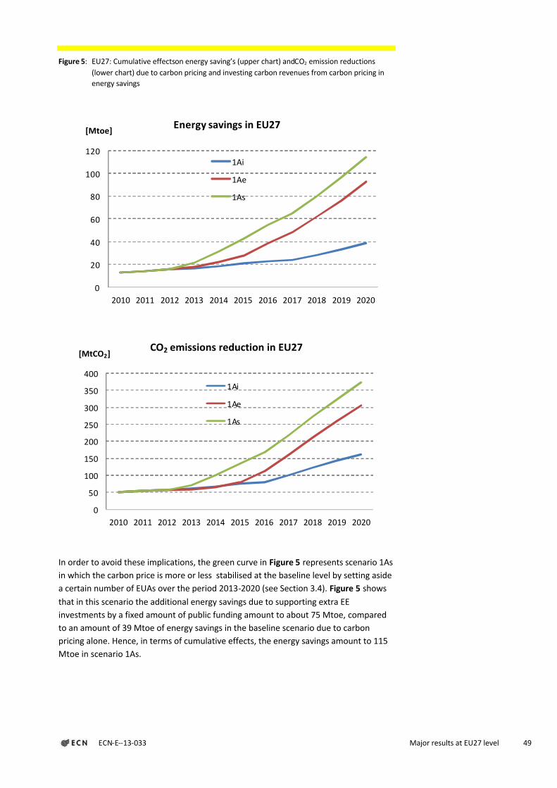
ECN-E--13-033 Major results at EU27 level 49
Figure 5: EU27: Cumulative effectson energy saving’s (upper chart) and CO2 emission reductions
(lower chart) due to carbon pricing and investing carbon revenues from carbon pricing in
energy savings
In order to avoid these implications, the green curve in Figure 5 represents scenario 1As
in which the carbon price is more or less stabilised at the baseline level by setting aside
a certain number of EUAs over the period 2013-2020 (see Section 3.4). Figure 5 shows
that in this scenario the additional energy savings due to supporting extra EE
investments by a fixed amount of public funding amount to about 75 Mtoe, compared
to an amount of 39 Mtoe of energy savings in the baseline scenario due to carbon
pricing alone. Hence, in terms of cumulative effects, the energy savings amount to 115
Mtoe in scenario 1As.
0
20
40
60
80
100
120
2010 2011 2012 2013 2014 2015 2016 2017 2018 2019 2020
[Mtoe]Energy savings in EU27
1Ai
1Ae
1As
0
50
100
150
200
250
300
350
400
2010 2011 2012 2013 2014 2015 2016 2017 2018 2019 2020
[MtCO2]CO2 emissions reduction in EU27
1Ai
1Ae
1As

In terms of CO2 emissions reduction, the impact of carbon pricing alone amounts to 162
MtCO2, the additional effects of energy savings investments amount to 144 MtCO2 in
scenario 1Ae and 211 MtCO2 in scenario 1As. Hence, the cumulative effects of both
carbon pricing and EE investments amount to 306 MtCO2 and 373 MtCO2 in scenarios
1Ae and 1As, respectively.14
Therefore, it may be concluded that the effects of carbon pricing on energy savings
and CO2 emissions reduction are substantially enhanced if (i) the revenues of carbon
pricing are used to support extra energy savings investments, and (ii) the resulting
decline in the ETS carbon price – i.e. due to the additional EE investments – is nullified
by setting aside a certain amount of emission allowances.
xxxxxxxxxxxxssssssssxxxxxxxxxxxxxx
14 Note that in scenario 1Ae, there is a reduction in CO2 emissions (and energy use) in the period 2013-2020 despite the existence of the ETS cap. This can be explained as follows. Due to additional EE investments the carbon price first declines to zero. Up to this point, additional EE investments do not reduce overall ETS emissions (and hardly energy use by ETS sectors). Beyond this point, however, further increasing EE investments does reduce overall ETS emissions (and energy use by ETS sectors), as there is no shifting anymore of emissions or energy use across ETS sectors within the cap. In scenario 1Ae the amount of additional EE investments is so large that the first part of these investments are not effective in reducing CO2 emissions (and energy use) by the ETS sectors – and only reduce the ETS carbon price – while beyond this point, the second part of these investments do become effective.

ECN-E--13-033 Summary of EU27 results across all scenarios 51
4Summary of EU27 results
across all scenarios
This Chapter provides a summary and graphical comparison of the main scenario results
at the EU27 level as discussed in the previous sections.
Figure 6: Energy savings in 2020 by sector and scenario (in Mtoe)
First of all, Figure 6 shows an overview of the energy savings in 2020 by sector and
scenario. Not surprisingly, the savings by sector vary widely across the scenarios
considered:
Industry: savings range from -5 Mtoe in scenario 2Ai (EEO, predominantly for
Households and Tertiary) to 20 Mtoe in 1Bi (30% GHG reduction), mainly due to the
level of the carbon price in these scenarios, i.e. 0 and 80 t/CO2, respectively.
1Bi 2Ai 2Bi 1Av 1Bv 2Av 2Bv 1Ae 1An 1As 2At
Other sectors 23 8 29 24 37 22 37 49 -1 59 10
Tertiary 1 9 10 11 10 14 14 2 18 2 9
Households 2 17 19 35 33 38 38 1 35 1 17
Industry 20 -5 16 6 11 6 11 1 1 13 -1
-20
0
20
40
60
80
100
120
[Mtoe]
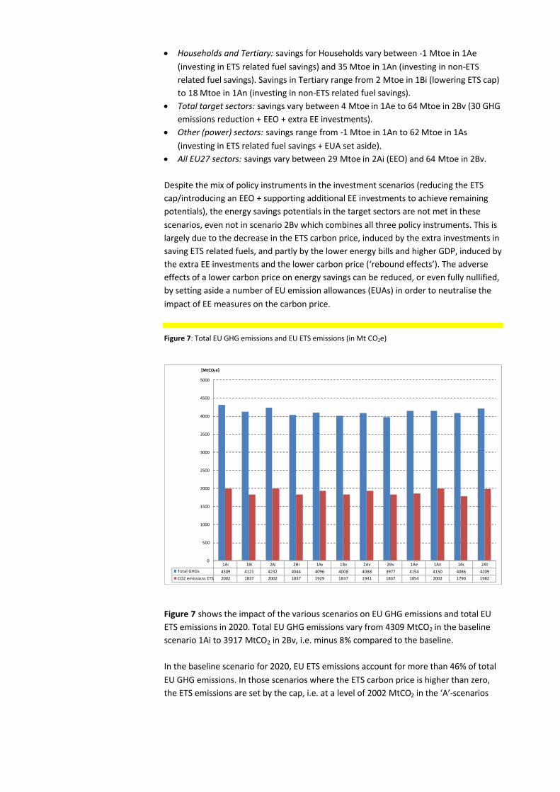
Households and Tertiary: savings for Households vary between -1 Mtoe in 1Ae
(investing in ETS related fuel savings) and 35 Mtoe in 1An (investing in non-ETS
related fuel savings). Savings in Tertiary range from 2 Mtoe in 1Bi (lowering ETS cap)
to 18 Mtoe in 1An (investing in non-ETS related fuel savings).
Total target sectors: savings vary between 4 Mtoe in 1Ae to 64 Mtoe in 2Bv (30 GHG
emissions reduction + EEO + extra EE investments).
Other (power) sectors: savings range from -1 Mtoe in 1An to 62 Mtoe in 1As
(investing in ETS related fuel savings + EUA set aside).
All EU27 sectors: savings vary between 29 Mtoe in 2Ai (EEO) and 64 Mtoe in 2Bv.
Despite the mix of policy instruments in the investment scenarios (reducing the ETS
cap/introducing an EEO + supporting additional EE investments to achieve remaining
potentials), the energy savings potentials in the target sectors are not met in these
scenarios, even not in scenario 2Bv which combines all three policy instruments. This is
largely due to the decrease in the ETS carbon price, induced by the extra investments in
saving ETS related fuels, and partly by the lower energy bills and higher GDP, induced by
the extra EE investments and the lower carbon price (‘rebound effects’). The adverse
effects of a lower carbon price on energy savings can be reduced, or even fully nullified,
by setting aside a number of EU emission allowances (EUAs) in order to neutralise the
impact of EE measures on the carbon price.
Figure 7: Total EU GHG emissions and EU ETS emissions (in Mt CO2e)
Figure 7 shows the impact of the various scenarios on EU GHG emissions and total EU
ETS emissions in 2020. Total EU GHG emissions vary from 4309 MtCO2 in the baseline
scenario 1Ai to 3917 MtCO2 in 2Bv, i.e. minus 8% compared to the baseline.
In the baseline scenario for 2020, EU ETS emissions account for more than 46% of total
EU GHG emissions. In those scenarios where the ETS carbon price is higher than zero,
the ETS emissions are set by the cap, i.e. at a level of 2002 MtCO2 in the ‘A’-scenarios
1Ai 1Bi 2Ai 2Bi 1Av 1Bv 2Av 2Bv 1Ae 1An 1As 2At
Total GHGs 4309 4121 4232 4044 4096 4008 4088 3977 4154 4150 4086 4209
CO2 emissions ETS 2002 1837 2002 1837 1929 1837 1941 1837 1854 2002 1790 1982
0
500
1000
1500
2000
2500
3000
3500
4000
4500
5000
[MtCO2e]

ECN-E--13-033 Summary of EU27 results across all scenarios 53
(20% EU GHG reduction in 2020) and 1837 MtCO2 in the ‘B’-scenarios (30% target).
However, in three ‘A’-scenarios (1Av, 2Av and 1Ae), actual ETS emissions in 2020 have
fallen below the cap, notably in scenario 1Ae (1854 MtCO2), resulting in a carbon price
equal to zero. Moreover, in two ‘A’-scenarios (1As and 2At), the ETS cap in 2020 is
actually reduced by setting aside a certain number of EUAs, for instance by 212 MtCO2
equivalents in 1As. Overall, across all scenarios, EU ETS emissions range from 2002
MtCO2 in the baseline to 1790 MtCO2 in 1As, i.e. minus 11% compared to – and in
addition to – the baseline.
Figure 8: ETS carbon price, 2012-2020 (in €/tCO2)
Figure 8 shows the evolution of the ETS carbon price over the period 2012-2020 for all
scenarios.15 As expected, the carbon price is highest – and far above the baseline trend
– in the four ‘B’-scenarios (all with a more stringent ETS cap), in particular in scenario
1Bi (with no additional EE measures reducing the carbon price; see Section 3.1 for
further discussion). In scenario 1An (investing in non-ETS related fuel savings), the
carbon price moves slightly above the baseline trend, while in scenario 2Ai (introducing
an EEO for Households and Tertiary), the carbon price declines slowly but steadily
below the baseline trend but remains positive (>0) up to 2020. As noted, however, in
three scenarios – 1Av, 2Av and 1Ae – the carbon price falls to zero, even amply before
2020.
xxxxxxxxxxxxssssssssxxxxxxxxxxxxxx
15 The carbon price of the two ‘EUA set aside’ scenarios (1As and 2At) is not presented separately as, due to the set asides, the evolution of the carbon price in these scenarios is similar to the trend in the baseline carbon price of scenario 1Ai.
2012 2013 2014 2015 2016 2017 2018 2019 2020
1Ai 16 16 16 16 16 17 17 17 17
1Bi 16 61 72 83 81 86 82 86 80
2Ai 16 16 16 15 13 12 11 10 9
2Bi 16 61 72 79 75 76 70 72 65
1Av 16 13 8 4 0 0 0 0 0
1Bv 16 58 61 66 60 55 45 44 36
2Av 16 13 9 5 1 0 0 0 0
2Bv 16 58 63 67 60 55 44 43 35
1Ae 16 11 4 0 0 0 0 0 0
1An 16 17 18 19 20 20 21 21 20
0
10
20
30
40
50
60
70
80
90
100
[€/tCO2]

Figure 9: Change in average household electricity bill in the EU27 by 2020 (in €)
Figure 9 illustrates the change in average household electricity bills across the various
scenarios, compared to the baseline. This change varies from an increase of € 61 in
scenario 1Bi (due to the pass-through of the higher carbon costs) to a significant
decrease of € 189 in scenario 1Ae (investing in ETS related fuel savings, resulting in less
power use, a zero carbon price and, hence, a lower power price). As the average
household power bill in 2020 amounts to € 678 in the baseline, these changes are equal
to +9% and -28% of this amount, respectively.
Figure 10 compares the annual average ETS auction revenues versus the public funding
needs to stimulate additional EE investments for achieving the remaining energy savings
potential in the target sectors up to 2020. Annual auction revenues vary from € 2 billion
in scenario 1Ae to € 86 billion in 1Bi (based on the carbon price above), while EE public
support needs range from € 3 billion in scenarios 2Bi and 2Bv to € 9 billion in scenarios
1Ae, 1An and 1As.
-250
-200
-150
-100
-50
0
50
100
1Bi 2Ai 2Bi 1Av 1Bv 2Av 2Bv 1Ae 1An 1As 2At
[€]
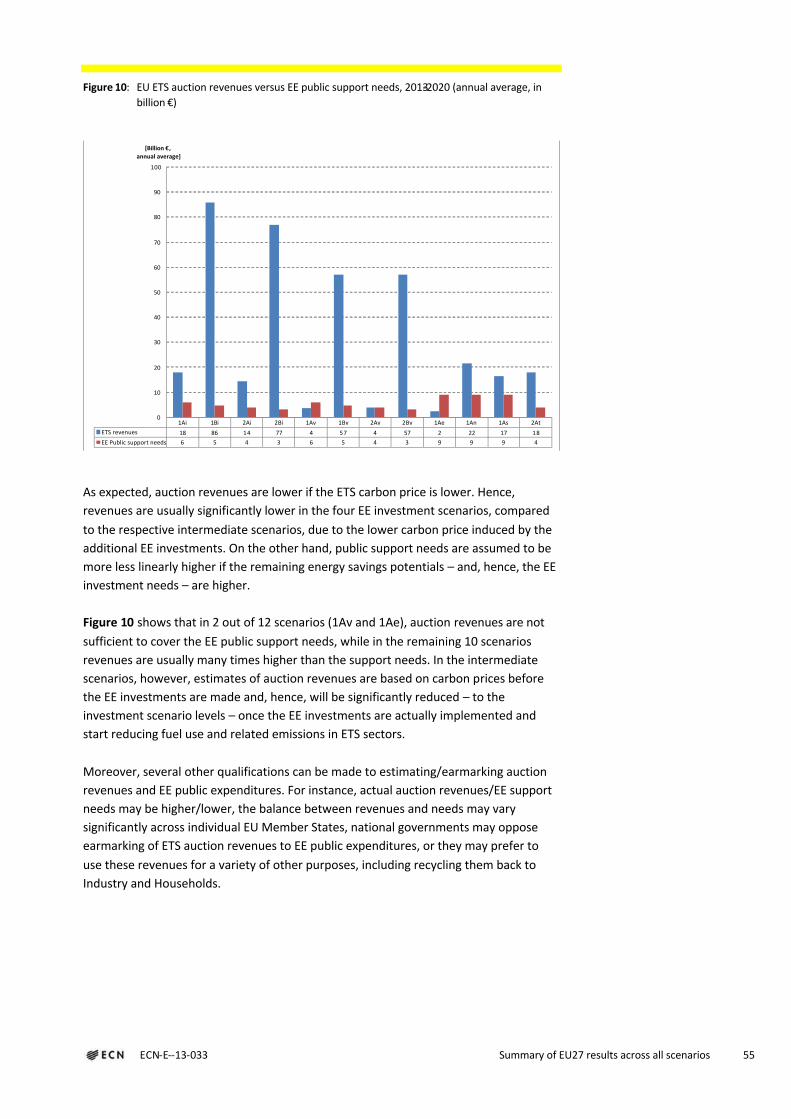
ECN-E--13-033 Summary of EU27 results across all scenarios 55
Figure 10: EU ETS auction revenues versus EE public support needs, 2013-2020 (annual average, in
billion €)
As expected, auction revenues are lower if the ETS carbon price is lower. Hence,
revenues are usually significantly lower in the four EE investment scenarios, compared
to the respective intermediate scenarios, due to the lower carbon price induced by the
additional EE investments. On the other hand, public support needs are assumed to be
more less linearly higher if the remaining energy savings potentials – and, hence, the EE
investment needs – are higher.
Figure 10 shows that in 2 out of 12 scenarios (1Av and 1Ae), auction revenues are not
sufficient to cover the EE public support needs, while in the remaining 10 scenarios
revenues are usually many times higher than the support needs. In the intermediate
scenarios, however, estimates of auction revenues are based on carbon prices before
the EE investments are made and, hence, will be significantly reduced – to the
investment scenario levels – once the EE investments are actually implemented and
start reducing fuel use and related emissions in ETS sectors.
Moreover, several other qualifications can be made to estimating/earmarking auction
revenues and EE public expenditures. For instance, actual auction revenues/EE support
needs may be higher/lower, the balance between revenues and needs may vary
significantly across individual EU Member States, national governments may oppose
earmarking of ETS auction revenues to EE public expenditures, or they may prefer to
use these revenues for a variety of other purposes, including recycling them back to
Industry and Households.
1Ai 1Bi 2Ai 2Bi 1Av 1Bv 2Av 2Bv 1Ae 1An 1As 2At
ETS revenues 18 86 14 77 4 57 4 57 2 22 17 18
EE Public support needs 6 5 4 3 6 5 4 3 9 9 9 4
0
10
20
30
40
50
60
70
80
90
100
[Billion €,
annual average]
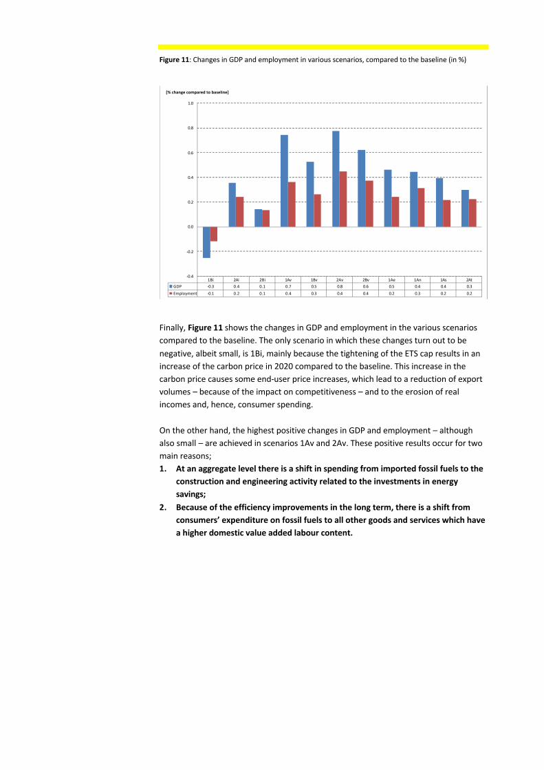
Figure 11: Changes in GDP and employment in various scenarios, compared to the baseline (in %)
Finally, Figure 11 shows the changes in GDP and employment in the various scenarios
compared to the baseline. The only scenario in which these changes turn out to be
negative, albeit small, is 1Bi, mainly because the tightening of the ETS cap results in an
increase of the carbon price in 2020 compared to the baseline. This increase in the
carbon price causes some end-user price increases, which lead to a reduction of export
volumes – because of the impact on competitiveness – and to the erosion of real
incomes and, hence, consumer spending.
On the other hand, the highest positive changes in GDP and employment – although
also small – are achieved in scenarios 1Av and 2Av. These positive results occur for two
main reasons;
1. At an aggregate level there is a shift in spending from imported fossil fuels to the
construction and engineering activity related to the investments in energy
savings;
2. Because of the efficiency improvements in the long term, there is a shift from
consumers’ expenditure on fossil fuels to all other goods and services which have
a higher domestic value added labour content.
1Bi 2Ai 2Bi 1Av 1Bv 2Av 2Bv 1Ae 1An 1As 2At
GDP -0.3 0.4 0.1 0.7 0.5 0.8 0.6 0.5 0.4 0.4 0.3
Employment -0.1 0.2 0.1 0.4 0.3 0.4 0.4 0.2 0.3 0.2 0.2
-0.4
-0.2
0.0
0.2
0.4
0.6
0.8
1.0
[% change compared to baseline]

ECN-E--13-033 Summary of EU27 results across all scenarios 57
References
Barker, T., A. Dagoumas, and J. Rubin (2009): “The macroeconomic rebound effect and
the world economy”, Energy Efficiency, Vol. 2, No. 4, pp. 411-427.
Chewpreecha, U., and H. Pollitt (2009): Extending the E3ME model to 2050: An
introduction to E3ME, Version 4.6, Cambridge Econometrics Working Paper.
Cowart, R. (2011): Prices and Policies: Carbon Caps and Efficiency Programmes for
Europe’s Low –Carbon Future, Regulatory Assistance Project (RAP), Brussels.
EC (1996): European System of Accounts ESA 1995, Eurostat, Brussels-Luxembourg.
EC (2008): EU energy trends to 2030 – Update 2007, European Commission, Directorate-
General for Energy, Brussels.
EC (2010a): Analysis of options to move beyond 20% greenhouse gas emission
reductions and assessing the risk of carbon leakage, Communication from the
Commission, COM(2010) 265 final, Brussels, 26 May 2010.
EC (2010b): Analysis of options to move beyond 20% greenhouse gas emission
reductions and assessing the risk of carbon leakage – Background information
and analysis, Part I, Commission Staff Working Document, SEC(2010) 650,
Brussels, 26 May 2010.
EC (2010c): Analysis of options to move beyond 20% greenhouse gas emission
reductions and assessing the risk of carbon leakage – Background information
and analysis, Part II, Commission Staff Working Document, SEC(2010) 650,
Brussels, 26 May 2010.
EC (2010d): EU energy trends to 2030 – Update 2009, European Commission,
Directorate-General for Energy, Brussels.
EC (2011a): Energy Efficiency Plan 2011, Communication from the Commission,
COM(2011) 109 final, Brussels, 8 March 2011)
EC (2011b): Impact Assessment, Commission Staff Working Paper, Accompanying the
Energy Efficiency Plan 2011, SEC(2011) 277 final, Brussels, 8 March 2011.
EC (2011c): The Commission’s new Energy Efficiency Plan – what is at stake?,
Memo/11/149, Brussels 8 March 2011.

EC (2011d): Proposal for a Directive on the European Parliament and of the Council on
energy efficiency and repealing Directives 2004/8/EC and 2006/32/EC,
COM(2011) 370 final, Brussels, 22 June 2011.
EC (2011e): Impact Assessment, Commission Staff Working Paper, Accompanying the
proposed Directive on Energy Efficiency, SEC(2011) 779 final, Brussels, 22 June
2011.
EC (2011f): Annexes to the Impact Assessment, Commission Staff Working Paper,
Accompanying the proposed Directive on Energy Efficiency, SEC(2011) 779
final, Brussels, 22 June 2011.
EC (2011g): The Commission’s new Energy Efficiency Directive – What is the objective?,
Memo/11/440, Brussels, 22 June 2011.
EC (2012): Non-Paper of the Services of the European Commission on Energy Efficiency
Directive, Informal Energy Council, Brussels, 19-20 April 2012.
ECF (2011): Energy Demand in the EU – A comparison of forecasts and ambitions, A
contributing research paper to ‘Energy Savings 2020: How to triple the impact
of energy saving policies in Europe’, European Climate Foundation, Brussels.
ECF and RAP (2011): Tapping Europe’s Efficiency Reservoir, Paper by the European
Climate Foundation (ECF) and the Regulatory Assistance Project (RAP) based on
their jointly commissioned study: “Energy Savings 2020: How to triple the
impact on energy savings policies in Europe”, Brussels.
Eichhammer, W., T. Fleiter, B. Schlomann, S. Faberi, M. Fioretto, N. Piccioni, S.
Lechtenböhmer, A. Schüring, and G. Resch (2009): Study on the Energy Savings
Potentials in EU Member States, Candidate Countries and EEA Countries, Final
Report to the EC, DG Energy and Transport, Fraunhofer ISI, Karlsruhe.
Pollitt, H. (2012): E3ME: An Energy-Environment-Economy Model for Europe, A Non-
Technical Description, Cambridge Econometrics.
Sijm, J., Hers, J., Lise, W., Wetzelaer, B. (2008): The impact of the EU ETS on electricity
prices, Final report to DG Environment of the European Commission, ECN-E--
08-007, Petten/Amsterdam.
Voogt, M., and W. Dubbeld (2012): Commercial energy services: a win-win combination,
Newsletter SQ Consult, June 2012.
Vivid Economics (2012): Carbon taxation and fiscal consolidation: the potential of
carbon pricing to reduce Europe’s fiscal deficits, report prepared for the
European Climate Foundation and Green Budget Europe, May 2012.
Wesselink, B., K. Blok, W. Eichhammer, and T. Boermans (2011): The upfront
investments required to double energy savings in the European Union in 2020’,
Report to the Regulatory Assistance Project (RAP) conducted by Ecofys and
Fraunhofer ISI, Ecofys, Utrecht, the Netherlands.
Wesselink, B., R. Harmsen en W. Eichhammer (2010): Energy Savings 2020: How to
triple the impact of energy savings policies in Europe, Report to the European
Climate Foundation (ECF) and the Regulatory Assistance Project (RAP)
conducted by Ecofys and Fraunhofer ISI, Brussels.

ECN-E--13-033 Summary of EU27 results across all scenarios 59
Appendix A. Policies included in the baseline scenario
The baseline scenario used in this study is based on the PRIMES 2009 Reference
Scenario (EC, 2010d). This Reference Scenario includes the following policies:
Regulatory measures – energy efficiency:
Eco-design Framework Directive 2005/32/EC;
Stand-by regulation 2008/1275/EC;
Simple Set-to boxes regulation 2009/107/EC;
Office/street lighting regulation 2009/245/EC
Household lighting regulation 2009/244/EC;
External power supplies regulation 2009/278/EC;
Labelling Directive 2003/66/EC;
Cogeneration Directive 2004/8/EC;
Directive 2006/32/EC on end-use energy efficiency and energy services;
Buildings Directive 2002/91/EC;
Energy Star Program (a voluntary labelling programme).
Regulatory measures – energy markets and power generation
Completion of the internal energy market;
EU ETS directive 2003/87/EC as amended by Directive 2008/101/EC and Directive
2009/29/EC;
Energy Taxation Directive 2003/96/EC;
Large Combustion Plant Directive 2001/80/EC;
IPPC Directive 2008/1/EC;
Directive of the geological storage of CO2 2009/31/EC;
Directive on national emissions’ ceilings for certain pollutants 2001/81/EC;
Water Framework Directive 20000/60/EC;
Landfill Directive 99/31/EC.
Transport
Regulation on CO2 from cars 2009/443/EC;
Regulative Euro 5 and 6 2007/715/EC;
Fuel Quality Directive 2009/30/EC;
Biofuels Directive 2003/30/EC;
Implementation of MARPOL Convention ANNEX VI.
Financial Support
TEN-E guidelines (Decision 1364/2006);
European Energy programme for Recovery (Regulation 2009/663/EC);

RTD Support;
State aid guidelines for Environmental Protection and 2008 Block Exemption
Regulation;
Cohesion Policy – ERDF, ESF and Cohesion Fund.
National measures
Strong nation RES policies;
Nuclear.
More details can be found in EU Energy Trends to 2030 – Update 2009 (EC, 2010d).

ECN-E--13-033 Summary of EU27 results across all scenarios 61
Appendix B. Estimation of energy savings potentials, investment needs and public funding
For each of the four intermediate scenarios (1Ai, 1Bi, 2Ai and 2Bi), the following input
variables have been estimated at both the EU27 level and the individual EU Member
State level:
The updated or remaining energy savings potentials up to 2020 for the three target
sectors of this study (Households, Industry and Tertiary);
The (private) investment needs to achieve these updated potentials;
The public funding or support assumed to be needed in order to induce these
(private) investments.
The methodology to achieve these input variables is explained below, including some
results (see also Sections 2.2 and 3.2 of the main text).
B.1. Energy savings potentials in the EU27
The Baseline scenario (1Ai)
The estimation of the energy savings potentials for the present study builds on the so-
called ‘Fraunhofer study’ for the European Commission (EC) on the energy savings
potentials in EU Member States (Eichhammer et al., 2009). The Fraunhofer study
provides estimates of energy savings potentials for the period 2005-2020 for three
types or cases of potentials, i.e. the so-called Low Policy Intensity (LPI) case, the High
Policy Intensity (HPI) case and the Technical Potentials case. These potentials are
detailed for end-use sectors, for fuel and electricity use, and for different applications.
In addition, we have used the more recent ‘Ecofys study’ for the European Climate
Foundation (ECF) on “Energy Savings 2020: How to triple the impact of energy savings
policies in Europe” (Wesselink et al., 2010) and the Regulatory Assistance Project (RAP)
study on “The upfront investments required to double energy savings in the European
Union in 2020” (Wesselink et al., 2011). In the Ecofys study (Wesselink et al., 2010),
which is based on the Fraunhofer study, potentials have been defined with regard to
the HPI case most of the time, but sometimes resemble the Technical Potentials case.

The Ecofys figures are not as detailed as those provided by the Fraunhofer study. For
this study, it has been assumed that the missing Ecofys figures are generally in line with
those for the HPI case.
The Fraunhofer/Ecofys potentials are defined against the Primes 2007 Baseline scenario
for the period 2005-2020. As explained in Section 2.1, however, an updated Primes
2009 Reference scenario has been published in 2009 which includes the impact of the
economic crisis since 2008, the implementation of more recent MS energy savings
policies and the (expected) higher energy prices up to 2020. Compared to the PRIMES
2007 scenario, this leads to a lower trend for energy consumption up to 2020. As a
result, part of the savings potentials identified by Fraunhofer/Ecofys is already used in
the Primes 2009 scenarios due to the higher energy prices and the extra policy
measures. Therefore, the estimates for the energy savings potentials have been
updated, using the increase in energy-intensity per sector as a proxy for the extra
savings. It has been assumed that the effect of higher energy prices and extra policy
only takes effect as of 2012. Overall, this results in 20-30% lower estimates of energy
savings potentials for the scenarios and sectors considered in this study (compared to
the earlier estimates by Fraunhofer/Ecofys).
In addition, if policy makers indeed want to use the ETS auction revenues to realize the
savings potentials this is only possible from about 2013 onwards, firstly because the
revenues start streaming in that year and, secondly, because it takes some time to set
up measures to stimulate extra savings. As a result, only part of the energy savings
potentials can actually be realized. This part was estimated per category of potentials,
based on saving options not applied over the past years and lost permanently (e.g., new
dwellings not built according to the Fraunhofer/Ecofys standards up to 2013), saving
options that can still be realized (e.g. refurbishment of existing buildings) and options
for which the period up to 2020 is too short to realize the potential (e.g. new industrial
processes; for more details, see Appendix C).
Per category of energy savings potentials, an effective starting year was assumed that
defined the part to be realized up to 2020. After this second correction the remaining
energy savings potentials in the baseline scenario 1Ai equal 40-50% of the original
potentials estimated by Fraunhofer/Ecofys (see Table 23 below).
The EU GHG stretch scenario (1Bi)
In scenario 1Bi, the target for EU GHG emission reduction in 2020 is 30% instead of 20%,
resulting in a higher ETS carbon price (see Section 3.1). Consequently, the extra
emission reduction is partly accomplished by extra energy savings, in particular in the
industrial ETS sectors. The higher carbon price raises the energy costs relatively the
most in industry because the base energy prices are relatively low compared to other
sectors. Therefore, most of the extra savings are found for Industry (12% of its energy
consumption). For Households only the electricity price increases – due to the pass-
through of the higher ETS carbon prices – and extra saving are much lower (3% of
household energy use up to 2020).
The extra industrial savings due to the higher ETS price are such that they more or less
equal the savings potential for this sector up to 2020. For the sectors Households and

ECN-E--13-033 Summary of EU27 results across all scenarios 63
Tertiary, the remaining potentials are still a considerable part of the original potentials
(see Table 23). For the relevant end-use sectors together (excluding transport) the
remaining savings potentials decrease to about 30% of the original Fraunhofer/Ecofys
potential.
Table 23: Energy saving potentials at EU27 level per scenario and target sector (in Mtoe and in % of
original Ecofysestimated potentials)
Households Tertiary Industry Total
In Mtoe
Primes-2007 79.2 34.5 46.4 160.1
Primes-2009 63.3 24.1 36.5 123.9
Scenario 1Ai 37.0 15.6 20.9 73.5
Scenario 1Bi 33.2 13.5 4.7 51.5
Scenario 2Ai 22.2 6.6 20.9 49.7
Scenario 2Bi 20.7 6.4 6.1 33.3
In % of original Ecofys estimated potentials, based on Primes-2007
Primes-2007 100 100 100 100
Primes-2009 80 70 79 77
Scenario 1Ai 47 45 45 46
Scenario 1Bi 42 39 10 32
Scenario 2Ai 28 19 45 31
Scenario 2Bi 26 19 13 21
The Energy Efficiency Obligation scenario (2Ai)
In scenario 2Ai, an Energy Efficiency Obligation of 1.5% per year for energy companies is
introduced which only refers to the sectors Households and Tertiary (see Section 2.1). It
is assumed, however, that not all of the EEO will necessarily be additional: if there are
already substantial energy savings in the baseline, e.g. 0.5% per annum, then we
assume that the EEO will only contribute an additional 1.0% per annum savings in
energy consumption in these sectors.
Compared to the estimated potentials, the extra savings due to the obligation are
assumed to be relatively large in the sectors Households and Tertiary. After correcting
potentials of scenario 1Ai for the EEO effect, the remaining savings potential for
households is not more than one-third of the original Ecofys estimate (see Table 23)
The EU GHG stretch and Energy Efficiency Obligation scenario (2Bi)
The scenario 2Bi combines the preceding scenarios of an Energy Efficiency Obligation
with the 30% GHG emissions reduction target. The effects of both policies will overlap,
but not entirely. For the non-ETS sectors Households and Tertiary the 30% target
mainly affects electricity use; the impact of the Energy Efficiency Obligation will focus
mostly on heating. For industry, the impact of the 30% target is much larger than the
EEO effect.
The resulting energy savings potentials as shares of the original Ecofys’ estimated
potentials are 26% for Households, 19% for Tertiary and only 13% for Industry (see
Table 23).
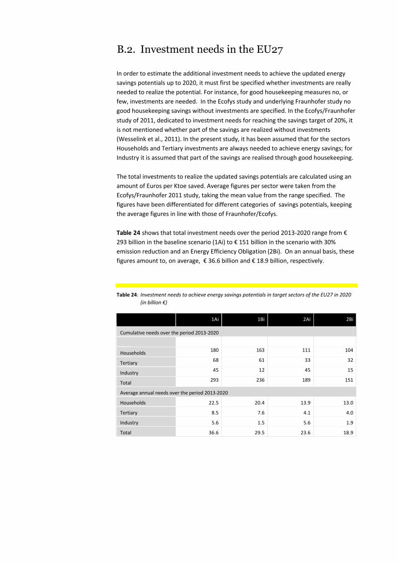
B.2. Investment needs in the EU27
In order to estimate the additional investment needs to achieve the updated energy
savings potentials up to 2020, it must first be specified whether investments are really
needed to realize the potential. For instance, for good housekeeping measures no, or
few, investments are needed. In the Ecofys study and underlying Fraunhofer study no
good housekeeping savings without investments are specified. In the Ecofys/Fraunhofer
study of 2011, dedicated to investment needs for reaching the savings target of 20%, it
is not mentioned whether part of the savings are realized without investments
(Wesselink et al., 2011). In the present study, it has been assumed that for the sectors
Households and Tertiary investments are always needed to achieve energy savings; for
Industry it is assumed that part of the savings are realised through good housekeeping.
The total investments to realize the updated savings potentials are calculated using an
amount of Euros per Ktoe saved. Average figures per sector were taken from the
Ecofys/Fraunhofer 2011 study, taking the mean value from the range specified. The
figures have been differentiated for different categories of savings potentials, keeping
the average figures in line with those of Fraunhofer/Ecofys.
Table 24 shows that total investment needs over the period 2013-2020 range from €
293 billion in the baseline scenario (1Ai) to € 151 billion in the scenario with 30%
emission reduction and an Energy Efficiency Obligation (2Bi). On an annual basis, these
figures amount to, on average, € 36.6 billion and € 18.9 billion, respectively.
Table 24: Investment needs to achieve energy savings potentials in target sectors of the EU27 in 2020
(in billion €)
1Ai 1Bi 2Ai 2Bi
Cumulative needs over the period 2013-2020
Households180 163 111 104
Tertiary68 61 33 32
Industry45 12 45 15
Total293 236 189 151
Average annual needs over the period 2013-2020
Households 22.5 20.4 13.9 13.0
Tertiary 8.5 7.6 4.1 4.0
Industry 5.6 1.5 5.6 1.9
Total 36.6 29.5 23.6 18.9

ECN-E--13-033 Summary of EU27 results across all scenarios 65
B.3. Public funding needs
The Fraunhofer/Ecofys potentials are claimed to be cost-effective, meaning that over
the life time of savings measures the annual energy cost savings compensate for the
investment costs annualised by means of a (social) discount rate. This rate, however, is
often lower that the (market) rate usually applied by private energy users. This
difference in social versus private discount rates – or other barriers to private energy
savings investments – may justify some public funding of these investments (assuming
that no other measures to address these barriers and to stimulate these investments
have already been implemented).
In order to estimate the public support assumed to be necessary to induce the (private)
investments to realise the updated energy savings potentials in the target sectors up to
2020, a default rate of 20% of gross investments has been assumed. For some parts of
energy savings, however, no or less funding has been assumed, e.g. for good
housekeeping in industry. Therefore, the average subsidy rate may vary across the
target sector analysed.
Table 25 shows that total investment needs over the period 2013-2020 range from €
47.3 billion in the baseline scenario (1Ai) to € 23.4 billion in the scenario with 30%
emission reduction and an Energy Efficiency Obligation ( 2Bi). On an annual basis, these
figures amount to, on average, € 5.9 billion and € 2.9 billion, respectively.
Table 25: Public funding needs to achieve energy savings potentials in target sectors of the EU27 in
2020 (in billion €)
1Ai 1Bi 2Ai 2Bi
Cumulative needs over the period 2013-2020
Households28.8 26.1 17.7 16.5
Tertiary12.5 11.6 6.6 6.4
Industry5.9 0.1 5.9 0.4
Total47.3 37.9 30.2 23.4
Average annual needs over the period 2013-2020
Households 3.6 3.3 2.2 2.1
Tertiary 1.6 1.5 0.8 0.8
Industry 0.7 0.0 0.7 0.1
Total 5.9 4.7 3.8 2.9
The figures in Table 25 can decrease when a smart stimulation system is introduced
that lowers the amount of funding for the same amount of investments. However, the
figures can also increase when it appears that more than 20% funding is needed to
realize investments into expensive or complicated saving options.

B.4. Energy savings potentials, investment needs
and public funding at the EU Member State
level
The updated energy saving potentials per country and per sector have been calculated
starting from the Fraunhofer database figures per country. These potentials have been
corrected both for the Primes 2009 Reference scenario effects and for the time passed
since 2005 up to 2013, using for each country the same approach and the same relative
cuts as made for the EU27 as a whole (as explained in Section B.1 above).
Table 26 shows the total energy saving potentials for the sectors Households, Tertiary
and Industry as a share of total energy end-use (including Transport) for each EU
Member State in 2020. In the baseline scenario, the updated potentials up to 2020 are
equal to about 4-6% of total energy end-use. In accordance with the earlier results at
the EU27 level (as discussed above), the shares are (much) lower for the other
scenarios.
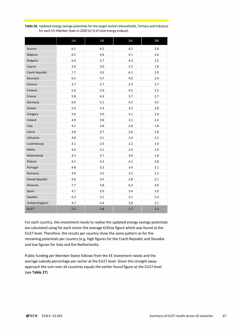
ECN-E--13-033 Summary of EU27 results across all scenarios 67
Table 26: Updated energy savings potentials for the target sectors (Households, Tertiary and Industry)
for each EU Member State in 2020 (in % of total energy end-use)
1Ai 1Bi 2Ai 2Bi
Austria 6.1 4.2 4.2 2.8
Belgium 6.2 4.6 4.1 3.0
Bulgaria 6.0 3.7 4.3 2.5
Cyprus 3.9 3.0 2.5 1.8
Czech Republic 7.7 3.9 6.1 2.9
Denmark 6.3 4.7 4.0 2.9
Estonia 3.7 2.7 2.4 1.7
Finland 5.6 2.9 4.5 2.2
France 5.8 4.3 3.7 2.7
Germany 6.9 5.1 4.5 3.2
Greece 5.4 4.3 3.2 2.6
Hungary 5.0 4.0 3.1 2.4
Ireland 4.9 3.8 3.1 2.4
Italy 4.1 2.8 2.8 1.8
Latvia 3.8 2.7 2.6 1.8
Lithuania 4.8 3.1 3.4 2.1
Luxembourg 3.1 2.0 2.2 1.4
Malta 4.0 3.1 2.5 1.9
Netherlands 4.2 2.7 3.0 1.8
Poland 6.1 4.3 4.1 2.8
Portugal 4.8 3.2 3.4 2.1
Romania 4.9 3.5 3.2 2.2
Slovak Republic 4.6 3.5 2.8 2.1
Slovenia 7.7 3.8 6.3 3.0
Spain 4.7 3.0 3.4 2.0
Sweden 6.3 3.1 5.1 2.4
United Kingdom 4.7 3.4 3.0 2.1
EU27 5.5 3.8 3.7 2.4
For each country, the investment needs to realise the updated energy savings potentials
are calculated using for each sector the average €/Ktoe figure which was found at the
EU27 level. Therefore, the results per country show the same pattern as for the
remaining potentials per country (e.g. high figures for the Czech Republic and Slovakia
and low figures for Italy and the Netherlands).
Public funding per Member States follows from the EE investment needs and the
average subsidy percentage per sector at the EU27 level. Given this straight away
approach the sum over all countries equals the earlier found figure at the EU27 level
(see Table 27)

Table 27: Public funding needs to achieve updated energy savings potentials in the target sectors per
EU Member State in 2020 (in million €)
1Ai 1Bi 2Ai 2Bi
Austria 1218 964 786 599
Belgium 1660 1368 1055 854
Bulgaria 449 332 298 206
Cyprus 58 49 36 30
Czech Republic 1206 754 861 475
Denmark 707 585 438 357
Estonia 96 80 60 49
Finland 749 469 539 299
France 6858 5707 4286 3520
Germany 10841 9005 6797 5566
Greece 1010 878 613 538
Hungary 787 673 481 412
Ireland 517 436 321 269
Italy 4183 3281 2690 2023
Latvia 152 122 97 76
Lithuania 183 140 120 86
Luxembourg 97 72 65 45
Malta 20 17 12 10
Netherlands 1443 1073 947 659
Poland 3014 2425 1907 1489
Portugal 685 523 448 324
Romania 1168 950 730 579
Slovak Republic 427 361 258 218
Slovenia 230 137 169 88
Spain 3472 2623 2281 1625
Sweden 1128 680 821 434
United Kingdom 4926 4045 3066 2466
EU27 47285 37751 30183 23296

ECN-E--13-033 Summary of EU27 results across all scenarios 69
Appendix C. Energy savings potentials, investment needs and public funding for buildings
This Appendix discusses some specific issues with regard to the estimation of energy
savings potentials, investment needs and public funding for buildings (including the
target sectors Households and Tertiary). These issues include:
Saving potentials;
Cost-effectiveness of savings;
Correction for late start of implementation;
Savings without investments;
Specific investment per category of savings;
Stimulation by funding or other means;
Amount of funding needed per category;
Alternative funding mechanism.
Saving potentials
As explained in Appendix B, the estimates of the updated energy savings potentials per
end-use sector are based on the Fraunhofer study/database for the cases LPI (Low
Policy Intensity), HPI (High Policy Intensity) and Technical (maximum potential). These
cases are detailed for fuel and electricity use and for different applications (Eichhammer
et al., 2009). Also available are more aggregated figures from the Ecofys study which is
said to be based on the HPI figures, but sometimes shows figures that look more like
the Technical potential (Wesselink et al., 2010).
In this Appendix, the Ecofys figures are used which are detailed as follows:
For saving potential categories regarding electricity the HPI figures are used because
overall electricity savings are the same for the Fraunhofer study and the Ecofys
study;
For other saving potential categories the HPI figures are scaled in such a way that
the total potential is equal to the Ecofys figures.
Cost-effectiveness
The HPI/Ecofys potentials are claimed to be cost-effective, meaning that over the life
time of saving measures the annual energy cost savings compensate for investment cost
that are annualized by means of a discount rate. This discount rate is lower than usually
applied by energy users (see Market versus HPI discount rates in Table 28). It is justified

by assuming that all kind of policies remove the barriers for investing in extra savings, in
fact closing the gap between market rates and HPI rates.
One direct way to close the gap between the discount rates is using ETS auction
revenues to subsidize investments for energy saving measures. The amount of subsidies
needed can be calculated as follows. For Households the discount rate of 4% leads to
yearly capital costs that are 77% of the capital cost for an 8% discount rate (see the
column “ratio” in Table 28 If market conditions prevail a subsidy that covers 23% of the
investments is needed to attain the same capital costs as in the HPI case. Similarly, for
Industry a subsidy of 62% can compensate for the higher market discount rate
compared to HPI.
Table 28: Subsidy rate to attain the lower capital costs assumed for HPI saving potentials
Market (LPI case) HPI case Ratio Subsidy
Life
time
Discount
rate
Annuitya Discount
rate
Annuitya Annuity
HPI/LPI
[years] [%] [€] [%] [€] [%] [%]
Households 15 8 11.7 4 9.0 77 23
Services 15 15 17.1 6 10.3 60 40
Industry 15 30 30.6 8 11.7 38 62
a) Based on an investment of € 100.
Source: Wesselink, et al., 2011).
Correction for late start of implementation
The Fraunhofer/Ecofys potentials regard the period from 2005 on and admit that less
savings can be realized if implementation is delayed (Wesselink et al., 2011). Using ETS
auction revenues to realize the savings potentials is only possible from about 2013 on.
Due to this late start only part of the potentials can be realized. For different categories
of energy savings potentials in the buildings sector, this has been assessed based on the
following considerations:A. Which saving options were not applied and are lost permanently?B. Which saving options that were not realized up till now can still be realized?C. For which saving options is the period up to 2020 too short to realize the potential?
Per category of energy savings potentials in buildings, these considerations apply as
follows:
New dwellings: Here consideration A is valid because new dwellings, once not build
with extra savings cannot contribute to extra savings in 2020.
Conversion: This regards mainly condensing boilers that are generally replaced every
15 years. Once not replaced by a condensing boiler the savings in 2020 are lost, thus
consideration A.
Refurbishment existing dwellings: The Fraunhofer study assumes an ambitious rate
for refurbishment (e.g. 3% of existing dwellings per year), resulting in substantial
savings. This rate has not been realized in past years but catching up is possible in
principle. However, the refurbishment capacity should be built up which takes time.
It will even be difficult to have the capacity in place for the regular 3% rate from
2013 on, let alone a rate of e.g. 5% for catching up. Therefore consideration A is

ECN-E--13-033 Summary of EU27 results across all scenarios 71
more relevant than consideration B, although consideration C applies for deep
renovation.
Water heating: This is often coupled to space heating when using a combi-boiler;
thus consideration A is valid. For other systems, e.g. separate fuel based systems
some catching up is possible, thus consideration B.
Household electric appliances: The Fraunhofer study assumes extra savings for
appliances due to the Ecodesign Directive that will specify minimum energy
efficiency standards in the period up to 2020. However, the process is delayed and
some savings are already lost and cannot be “repaired” before 2020, thus
consideration A. It is not clear whether savings beyond the standard are assumed;
here also consideration A is valid.
Heating new buildings: Here consideration A holds, as for new dwellings, but with
some catching up as the new buildings not built due to the economic crisis are built
later and have the extra savings as assumed in the Fraunhofer study (consideration
B).
Heating existing buildings: Here the ambitious refurbishment rate has not been
realized in past years. As for dwellings the refurbishment capacity has to be
expanded substantially even to reach the assumed level in coming years. Possibly
the rate could expand further up to 2020 to have some catching up (this mainly
consideration A, and partly consideration B).
Office lighting: Some catching up is possible if the replacement of old systems is
speeded up, thus consideration B.
HVAC: Coupled to refurbishment of buildings, thus same consideration B.
Street lighting: Here some catching up is possible if replacement of old systems is
speeded up, thus consideration B.
Savings without investments
In order to calculate investments it must be specified first whether investments are
really needed to realize the potential. E.g. for good housekeeping measures no, or few,
investments are needed (Wesselink et al., 2010 and 2011). Savings without investments
in buildings are possible for:
Heating existing dwellings;
Water heating;
Overall household electricity use;
Heating of existing buildings;
Office lighting.
Good housekeeping savings measures in business can yield 10-20% savings, but this is a
one-time gain in a period of 20 years. For households the savings are in the range of 3-
10%, but the higher figures ask for intensive efforts to change behaviour which raise the
cost for government. Good-housekeeping is, in general, very cost-effective for the
energy users and does not need subsidies, but some government money is often
needed to overcome so-called ‘hidden costs’ to realize energy savings potentials in
buildings.
Because the Ecofys study does not discuss energy savings in buildings due to
behavioural changes, it is assumed that always investments are needed to realize the
saving potentials.

Specific investments per category
The total investments per category of savings potential are calculated using specific
investment figures in €/Ktoe saved. Average figures for buildings as a whole are
available from the recent study by Ecofys (Wesselink et al., 2011). This study shows a
large range for investment needs (€ 350-650 billion for about 100 Mtoe of energy
savings). For the average specific investments the mean value has been taken (5000
€/Ktoe).
The figures must be diversified for the categories in the sectors Households and
Tertiary, keeping the average figure in line with that of Fraunhofer/Ecofys. The
following assumptions were made:
New dwellings: Higher than average specific investments.
Conversion: Relatively low specific investments for condensing boilers, but not very
low due to the decreasing energy demand for space heating.
Refurbishment existing dwellings: Average specific investments as this category
represents the majority of savings and investments.
Water heating: Less than average specific investments, in line with the condensing
boiler figures.
Household electric appliances: Rather low specific investments, but higher than in
the past due to increasing efforts needed to realize extra savings.
Heating new buildings: Higher than average specific investments, but lower than for
households due to the economic considerations in the Service sector.
Heating existing buildings: Average specific investments as it regards relatively
costly refurbishment and this category contributes substantially to the total savings
and investments for buildings.
Office lighting: Relatively low specific investments when refurbishment is coupled to
renovation.
HVAC: Relatively low specific investments when refurbishment is coupled to
renovation.
Street lighting: Relatively low specific investments when refurbishment is coupled to
renovation for traffic management reasons.
Stimulation by funding or other means
In the baseline scenario, savings are already stimulated by different types of policy
measures, e.g. regulation for appliances and new dwellings, information for changing
energy-use behaviour and subsidies on insulation of existing dwellings. In order to
realize the extra savings potentials different additional policy measures can be applied
per category of potential. However, the central objective of this study is to show the
effects of spending ETS auction revenues on extra savings. To this end the variant with
spending auction revenues on energy savings is compared to the baseline scenario,
keeping all other policy measures the same. Therefore, in this study we have only
analysed the opportunities for additional energy savings in buildings (i.e. in Households
and Tertiary) to be achieved by additional public support (funded form ETS auction
revenues) while ignoring alternative policies such as additional regulation or extra
information/awareness campaigns.
If there is a lack of auction revenues, however, it seems sensible to give priority to
categories of energy savings where there are no easy policy alternatives, such as
regulation. Therefore it is still worth to specify possibilities for alternative stimulation:

ECN-E--13-033 Summary of EU27 results across all scenarios 73
Heating existing dwellings: further regulation for insulation and boilers;
Heating new dwellings: regulation for Near Zero energy dwellings;
Appliances and lighting: further regulation?
Heating of existing buildings: further regulation for insulation and boilers;
Office lighting: further regulation?
Street lighting: further regulation?
Alternative funding mechanisms
Instead of subsidies on investments, alternative stimulation systems can lower the
amount of funding needed, e.g. a revolving fund providing soft loans. This solves at the
same time the financing problem and the economic attractiveness of the saving
measure. Especially for companies this approach can remove barriers and lower the
high market discount rate that they normally use for saving investments.
Amount of funding needed
In order to calculate the public funding needs a default rate of 20% subsidy has been
assumed. This is in line with current practices and the amount of subsidy to bridge the
gap between market discount rates and the rate applied for the cost-effective HPI
potentials (see Table 28). For Services bridging the gap between the market discount
rate and the assumed HPI rate asks for more than 20% subsidy. Here the alternative
policy measures indicated above can limit the subsidy to 20% instead of the higher
figures in Table 28.

ECN
Westerduinweg 3 P.O. Box 1
1755 LE Petten 1755 LG Petten
The Netherlands The Netherlands
T +31 88 515 4949
F +31 88 515 8338
info@ ecn.nl
www.ecn.nl