Investigation of two-fluid methods for Large Eddy

Simulation of spray combustion in Gas Turbines

Boileau M.1, Pascaud S.2, Riber E.1−3, Cuenot B.1,

Gicquel L.Y.M.1 and Poinsot T.J.3

October 29, 2007

1CERFACS, 42 avenue Gaspard Coriolis, 31057 Toulouse Cedex 01, France

2 Now at TURBOMECA (Safran Group), Pau, France

3IMFT (UMR CNRS-INPT-UPS 5502), Toulouse, France

1

Abstract

An extension of the Large Eddy Simulation (LES) technique to two-phase

reacting flows, required to capture and predict the behavior of industrial burn-

ers, is presented.

While most efforts reported in the literature to construct LES solvers for

two-phase flow focus on Euler-Lagrange formulation, the present work ex-

plores a different solution (’two-fluid’ approach) where an Eulerian formula-

tion is used for the liquid phase and coupled with the LES solver of the gas

phase. The equations used for each phase and the coupling terms are pre-

sented before describing validation in two simple cases which gather some

of the specificities of real combustion chamber: (1) a one-dimensional lam-

inar JP10/air flame and (2) a non-reacting swirled flow where solid particles

disperse [1]. After these validations, the LES tool is applied to a realistic

aircraft combustion chamber to study both a steady flame regime and an ig-

nition sequence by a spark. Results bring new insights into the physics of

these complex flames and demonstrate the capabilities of two-fluid LES.

Keywords: Spray combustion, Turbulence, Large Eddy Simulation, Gas tur-

bines.

2

1 Introduction

RANS (Reynolds Averaged Navier Stokes) equations are routinely solved to design

combustion chambers, for both gaseous and liquid fuels. Recently, in order to pro-

vide better accuracy for the prediction of mean flows but also to give access to un-

steady phenomena occurring in combustion devices (such as ignition, instabilities,

flashback or quenching), Large-Eddy Simulation (LES) has been extended to react-

ing flows. As shown by the numerous examples published in the last years [2–12],

this approach is very accurate in complex turbulent gaseous flows. This mainly

results from the explicit and direct computation of the largest scale structures of

the flow, which are the most difficult to model and contain a significant part of the

physics controlling the flame.

However most LES calculations consider only gaseous flows and flames. The

introduction of a dispersed liquid fuel raises two kinds of problems:

• The physics of a liquid fuel spray is very complex and is not yet fully un-

derstood [13]. The atomization process of a liquid fuel jet [14–18], the

turbulent dispersion of the resulting droplets [19–23], their interaction with

walls [24, 25], their evaporation and combustion [26] are phenomena occur-

ing for LES at the subgrid scale and therefore requiring accurate modelling.

• The numerical implementation of two-phase flow in LES remains a chal-

lenge. The equations for both gaseous and dispersed phases must be solved

together at each time step in a strongly coupled manner. This differs again

from classical RANS where both phases can be solved in a weakly coupled

procedure, bringing first the gas flow to convergence, then calculating the

associated dispersed phase and iterating until convergence of both phases.

Attempts to extend RANS formulation to LES of two-phase combustion may be

found in [7, 27–30]. They are all based on a Euler-Lagrange (EL) description of

3

the dispersed phase in which the flow is solved using an Eulerian method and the

particles are tracked with a Lagrangian approach. An alternative is the Euler-Euler

(EE) description, also called two-fluid approach, in which both the gas and the

dispersed phases are solved using an Eulerian formulation.

In RANS codes, the weak numerical coupling of the phases makes the EL

method well suited for gas turbine computations, but RANS with the EE approach

may also be found for example in simulations of fluidized beds [31,32] or chemical

reactors [33–35], two examples of two-phase flows with a high load of particles.

The experience gained in the development of RANS has led to the conclusions

that both approaches are useful and they are both found today in most commer-

cial codes. Moreover, coupling strategies between EE and EL methods within the

same application are considered for certain cases. In the framework of LES of gas

turbines, it is interesting to compare again EL or EE formulations.

Following the individual trajectory of millions of droplets created by standard

injectors implies computer resources that are still far beyond the capacities of com-

puters available today and even in the coming years. To overcome this problem the

stochastic Lagrangian approach is usually introduced, where each particle is only a

”numerical” particle, representing in fact a statistically homogeneous group of real

particles. This reduces the number of particles to compute but implies modelling

for these parcels of particles [36]. Moreover in order to reach the accuracy required

by LES, the stochastic Lagrangian approach must still involve an important num-

ber of particles that make it CPU time-consuming. Another difficult point is that

the topology of the flow in dense zones (like near the injectors) differs from a cloud

of droplets and a Lagrangian description is not adapted there. Finally the computer

implementation of the EL approach is not well-suited to parallel computers: since

two different solvers must be coupled, the complexity of the implementation on

a parallel computer increases drastically compared to a single-phase code. Two

4

methods may be used for LES: (1) task parallelization in which certain proces-

sors compute the gas flow and others compute the droplets flow and (2) domain

partitioning in which droplets are computed together with the gas flow on geomet-

rical subdomains mapped on parallel processors. Droplets must then be exchanged

between processors when leaving a subdomain to enter an adjacent domain. For

LES, it is easy to show that only domain partitioning is efficient on large grids

because task parallelization would require the communication of very large three-

dimensional data sets at each iteration between all processors. However, codes

based on domain partitioning are difficult to optimize on massively parallel archi-

tectures when droplets are clustered in one part of the domain (typically, near the

fuel injectors). Moreover, the distribution of droplets may change during the com-

putation: for a gas turbine re-ignition sequence, for example, the chamber is filled

with droplets when the ignition begins thus ensuring an almost uniform droplet

distribution; these droplets then evaporate rapidly during the computation, leaving

droplets only in the near injector regions. To preserve a high parallel efficiency

on thousands of processors, dynamic load-balancing strategies are required that

re-decompose the domain during the computation itself [30].

The EE approach has the important advantage to be straightforward to imple-

ment in a numerical tool, and immediately efficient as it allows the use of the same

parallel algorithm than for the gas phase [37]. However it requires an initial mod-

elling effort much larger than in the EL method [38] and faces difficulties in han-

dling droplet clouds with extended size distributions [39]. Moreover the resulting

set of equations is numerically difficult to handle and requires special care [40].

Throughout this paper, two-phase flows will be treated like monodisperse sprays,

an assumption which is not mandatory in EE methods but which makes their im-

plementation easier. Results also suggest that in many flows (see for example sec-

tion 4), this assumption is reasonable. Considering the lack of information on size

5

distribution at an atomizer outlet in a real gas turbine, this assumption might be

a reasonable compromise in terms of complexity and efficiency: tracking multi-

disperse sprays with precision makes sense only if the spray characteristics at the

injection point are well known. In most cases, droplets are not yet formed close

to the atomizer outlet anyway and even the Lagrange description faces difficulties

there.

In the context of LES, a new modelling issue appears for two-phase flow sim-

ulations, either in the EL or EE formulation, and is linked to the subgrid scale

model for the turbulent droplet dispersion. This problem has already been ad-

dressed in [41, 42] but is still an open question. However in the case of reacting

flows, turbulent droplet dispersion occurs in a very limited zone between the at-

omizer and the flame and it is greatly influenced by the flame dynamics, therefore

limiting the impact of the subgrid scale model.

The EE methodology in LES used throughout this work is taken from previous

work [38, 40, 43, 44] where the validity and limitations have been discussed exten-

sively, and it is not the purpose here to discuss further theoretical aspects. Despite

the known limitations of such methodology, it is interesting to evaluate the poten-

tial and accuracy of the existing models when applied to realistic geometries and

flows. This is the objective of the present paper, in the case of aeronautical gas

turbines.

The framework and the basic equations for the EE description are first recalled

in Section 2. The LES filtering procedure for these equations is described in Sec-

tion 2.5 along with the closure assumptions and models for subgrid terms, includ-

ing turbulent combustion. Simple validation cases are then presented: the lami-

nar two-phase one-dimensional flame and the dispersion of particles in a turbulent

swirled flow [1] are described in Section 3 and Section 4 respectively. The final

application is a sector of a gas turbine burner for which both the steady flow and

6

an ignition sequence using a spark discharge are computed in Sections 5.2 and 5.3

respectively.

2 Equations

2.1 Carrier phase

The set of instantaneous conservation equations in a multi-species reacting gas can

be written:∂w∂t

+∇ · F = Sc + Sl (1)

where w is the vector of the gaseous conservative variables w = (ρu, ρv, ρw, ρE, ρk)T

with respectively ρ, u, v, w, E, ρk the density, the three Cartesian components

of the velocity vector u = (u, v, w)T , the total energy per unit mass defined by

E = 12u · u + Ei where Ei is the internal energy, and ρk = ρYk where Yk is

the mass fraction of species k. It is usual to decompose the flux tensor F into an

inviscid and a viscous component: F = F(w)I + F(w,∇w)V . The three spatial

components of the inviscid flux tensor F(w)I are:

ρu2 + P ρuv ρuw

ρuv ρv2 + P ρvw

ρuw ρvw ρw2 + P

(ρE + P )u (ρE + P )v (ρE + P )w

ρku ρkv ρkw

(2)

where the hydrostatic pressure P is given by the equation of state for a perfect gas:

P = ρ r T , with the gas constant r = RW =

∑Nk=1

YkWkR andR = 8.3143 J/(mol.K)

the universal gas constant. The internal energy Ei is linked to the temperature

through the heat capacity of the mixture calculated as Cp =∑N

k=1 Yk Cp,k.

7

The components of the viscous flux tensor F(w,∇w)V take the form:

−τxx −τxy −τxz

−τxy −τyy −τyz

−τxz −τyz −τzz

−u · τx + qx −u · τy + qy −u · τz + qz

Jx,k Jy,k Jz,k

(3)

It is composed of the stress tensor τ = 2µ(S − 1/3 δijTr(S)) (momentum

equations), the energy flux u · τ + q (energy equation) and the diffusive flux Jk

(species equations). In the stress tensor expression, S = 1/2(∇ · u + (∇ · u)T )

is the deformation matrix and µ is the dynamic viscosity following a classical

power law. The diffusive flux of species k includes a correction velocity V c

that guarantees mass conservation, so that Jk = −ρ(Dk

WkW ∇Xk − YkV

c)

with

V c =∑N

k=1 DkWkW ∇Xk, Xk being the molar fraction of species k. The mix-

ture diffusion coefficient for species k is computed as Dk = µρ Sck

where the

Schmidt number Sck is a constant. Finally the heat flux vector q follows a Fourier’s

law and includes an additional term due to heat transport by species diffusion:

q = −λ∇T +∑N

k=1 Jkhs,k, where λ = µCp/Pr is the heat conduction coeffi-

cient of the mixture, with the Prandtl number Pr fixed at a constant value.

The chemical part of the source term Sc on the right hand side of Eq. (1) adds

a term to the energy equation (ωT ) and to the species equations (ωk). Chemistry is

described by M reactions involving the N reactants Mk as follows:

N∑k=1

ν ′kjMk ⇀↽N∑

k=1

ν ′′kjMk, j = 1,M (4)

The production/consumption rate ωk for species k is the sum of the reaction rates

ωkj produced by all M reactions:

ωk =M∑

j=1

ωkj = Wk

M∑j=1

νkjQj (5)

8

where νkj = ν ′′kj − ν ′kj and Qj is the rate of progress of reaction j and is written:

Qj = Kf,j

N∏k=1

(ρYk

Wk

)ν′kj

−Kr,j

N∏k=1

(ρYk

Wk

)ν′′kj

(6)

The forward reaction rate follows an Arrhenius law: Kf,j = Af,j exp(−Ea,j

RT

)where Af,j and Ea,j are the pre-exponential factor and the activation energy. The

reverse reaction rate is deduced from the equilibrium relation Kr,j = Kf,j/Keq

where Keq is the equilibrium constant.

The heat release is calculated from the species production/consumption rates

as:

ωT = −N∑

k=1

ωk∆h0f,k (7)

where ∆h0f,k is the formation enthalpy of species k.

The second part of the source term Sl is associated to the liquid phase through

the drag force and the evaporation. It adds a vector I to the right hand side of the

momentum equations, a heat transfer term Π on the energy equation and a mass

transfer term Γ on the fuel equation (see Section 2.3).

2.2 Dispersed phase

Eulerian equations for the dispersed phase may be derived by several means. A

popular and simple way consists in volume filtering of the separate, local, instan-

taneous phase equations accounting for the inter-facial jump conditions [45]. Such

an averaging approach may be restrictive, because particle sizes and particle dis-

tances have to be smaller than the smallest length scale of the turbulence. Besides,

it does not account for the Random Uncorrelated Motion (RUM), which measures

the deviation of particles velocities compared to the local mean velocity of the

dispersed phase [38] (see section 2.4). In the present study, a statistical approach

analogous to kinetic theory [46] is used to construct a probability density function

(pdf) fp(cp, ζp, µp,x, t) which gives the local instantaneous probable number of

9

droplets with the given translation velocity up = cp, the given mass mp = µp

and the given temperature Tp = ζp. The resulting model leads to conservation

equations having the same form than for the gas phase, for the particle number

density nl, the volume fraction αl, the correlated velocity ul (see section 2.4) and

the sensible enthalpy hs,l (supposed uniform in the droplet, so that in particular the

interface temperature Tζ is equal to the liquid temperature Tl). For a monodisperse

spray, neglecting droplets interaction terms, the conservation equations read:

∂

∂tnl +

∂

∂xjnlul,j = 0 (8)

∂

∂tρlαl +

∂

∂xjρlαlul,j = −Γ (9)

∂

∂tρlαlul,i +

∂

∂xjρlαlul,iul,j = Fd,i − ul,iΓ−

∂

∂xjρlαlδRl,ij (10)

∂

∂tρlαlhs,l +

∂

∂xjρlαlhs,lul,j = −(Φ + Γhs,F (Tl)) (11)

In these equations, the momentum and heat phase exchange source terms are split

in two parts : I = −Fd + ulΓ includes both the drag force and a momentum

transfer due to the mass transfer, and Π = Φ + Γhs,F (Tl), where hs,F (Tl) is

the fuel vapor enthalpy taken at the interface temperature Tl, includes conduction

and heat transfer linked to the mass transfer. The tensor δRl,ij corresponds to the

random uncorrelated motion (RUM) and is explained in section 2.4.

Note that without source terms (i.e. without evaporation, drag and RUM) the

momentum equation Eq. 10 is similar to the Burger’s equation, known to create

shock-like velocity gradients and therefore difficult to handle numerically. The ab-

sence of an isotropic pressure-like force can also lead to very high droplet number

density gradients. Such behaviors are unphysical and should be avoided. To this

purpose it is necessary to add stabilisation terms to this equation. This is explained

in section 2.6. Consequently the final Eulerian model without RUM is strictly

valid only for small Stokes number droplets, that behave like tracers and do not

form sharp number density gradients.

10

It has been shown in [47] that the resulting set of equations Eqs. 8 to 11 leads

to solutions similar to Lagrangian solutions in the case of a two-phase turbulent

channel flow.

2.3 Phase exchange source terms

Mass transfer between the gas and the liquid phases is linked to evaporation, which

follows the classical Spalding model [48]. Assuming that the dispersed phase is

composed of spherical droplets of pure fuel (denoted with the subscript F ), the

evaporation rate may be written as :

Γ = πnldSh(ρDF )ln(1 + BM ) (12)

where d is the droplet diameter, DF is the fuel vapor diffusivity and Sh is the Sher-

wood number that takes into account convective and turbulent effects. A commonly

used expression for this number is Sh = 2.0 + 0.55Re1/2d Sc

1/3F where Rep =

d|u − ul|/ν is the particle Reynolds number and ScF is the fuel vapor Schmidt

number. In this definition ν is the carrier phase kinematic viscosity. In Eq. (12),

one important parameter is the Spalding number BM = (YF,ζ − YF )/(1 − YF,ζ)

where YF,ζ is the fuel mass fraction at the droplet surface, calculated from the fuel

vapor partial pressure at the interface pF,ζ which is evaluated from the Clausius-

Clapeyron relation:

pF,ζ = pcc exp

(WF Lv

R

(1

Tcc− 1

Tl

))(13)

The reference pressure and temperature pcc and Tcc correspond to the saturation

conditions, and Lv is the latent heat of vaporisation.

The drag force is expressed as:

Fd =ρlαl

τp(ui − ul,i) (14)

11

introducing the particle relaxation time τp:

τp =4ρld

2

3ρνCdRed(15)

itself based on the drag coefficient Cd, which is 0.44 for Red greater than 1000 and

is defined by Cd = 24Red

(1 + 0.15 Re0.687d ) otherwise.

Finally, the conductive flux Φ through the interface is calculated as Φ = πnldλ

Nu(Tl − T ). In this expression, λ is the carrier phase conductivity and Nu is

the Nusselt number usually expressed similarly to the Sherwood number: Nu =

2.0 + 0.55Re1/2d Pr1/3.

2.4 The Random Uncorrelated Motion (RUM)

The averaging operation for the liquid droplet velocity described in the previous

section introduces a particle velocity deviation from the mean (or correlated) ve-

locity, noted u′′p = up − ul, and named the random uncorrelated velocity [38]. By

definition the statistical average (based on the particle probability density function)

of this uncorrelated velocity is zero: < u′′p >= 0. A conservation equation can be

written for the associated kinetic energy δθl =< u′′p,iu′′p,i > /2:

∂

∂tρlαlδθl +

∂

∂xjρlαlul,jδθl = −1

2∂

∂xjρlαlδSl,iij −

2 nl

τpδθl

− ρlαlδRl,ij∂ul,i

∂xj− Γδθl (16)

where unclosed terms δRl,ij and δSl (called here RUM terms) appear. However

the modelling of these terms as proposed for example in [47, 49, 50] is not yet

satisfactory and it is still an open and difficult question. In [47, 50] it has been

shown that in a configuration representative of industrial flows, the RUM is not

essential to capture the mean fields (velocity and mass flux) of the liquid phase, but

only influences the particle turbulent agitation. It has been therefore omitted in the

applications presented later in the paper.

12

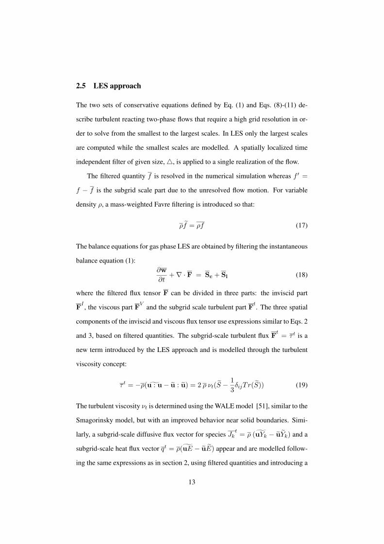
2.5 LES approach

The two sets of conservative equations defined by Eq. (1) and Eqs. (8)-(11) de-

scribe turbulent reacting two-phase flows that require a high grid resolution in or-

der to solve from the smallest to the largest scales. In LES only the largest scales

are computed while the smallest scales are modelled. A spatially localized time

independent filter of given size, 4, is applied to a single realization of the flow.

The filtered quantity f is resolved in the numerical simulation whereas f ′ =

f − f is the subgrid scale part due to the unresolved flow motion. For variable

density ρ, a mass-weighted Favre filtering is introduced so that:

ρf = ρf (17)

The balance equations for gas phase LES are obtained by filtering the instantaneous

balance equation (1):∂w∂t

+∇ · F = Sc + Sl (18)

where the filtered flux tensor F can be divided in three parts: the inviscid part

FI , the viscous part FV and the subgrid scale turbulent part Ft. The three spatial

components of the inviscid and viscous flux tensor use expressions similar to Eqs. 2

and 3, based on filtered quantities. The subgrid-scale turbulent flux Ft = τ t is a

new term introduced by the LES approach and is modelled through the turbulent

viscosity concept:

τ t = −ρ(u : u− u : u) = 2 ρ νt(S −13δijTr(S)) (19)

The turbulent viscosity νt is determined using the WALE model [51], similar to the

Smagorinsky model, but with an improved behavior near solid boundaries. Simi-

larly, a subgrid-scale diffusive flux vector for species Jkt = ρ (uYk − uYk) and a

subgrid-scale heat flux vector qt = ρ(uE − uE) appear and are modelled follow-

ing the same expressions as in section 2, using filtered quantities and introducing a

13

turbulent diffusivity Dtk = νt/Sct

k and a thermal diffusivity λt = µtCp/Prt. The

turbulent Schmidt and Prandtl numbers are fixed to 1 and 0.9 respectively.

In turbulent reacting cases the Dynamically Thickened Flame model [52–55] is

used, where a thickening factor F is introduced to thicken the flame front and the

efficiency function E developed by Colin et al. [4] is used to account for subgrid

scale wrinkling.

For the dispersed phase, filtered conservative variables and equations are built with

the same methodology as for the carrier phase and similarly a particle subgrid stress

tensor τ tl,ij appears :

τ tl,ij = −nl( ul,iul,j − ul,iul,j) (20)

where the Favre filtered quantities fl are defined as nlfl = nlfl. By analogy to

compressible single phase flows [56, 57], Riber et al. propose a viscosity model

for the SGS tensor Tl,ij [44]. The trace-free SGS tensor is modeled using a vis-

cosity assumption (compressible Smagorinsky model), while the subgrid energy is

parametrized by a Yoshizawa model [58] :

τ tl,ij = CS,l2∆2nl|Sl|(Sl,ij −

δij

3Sl,kk)− CV,l2∆2nl|Sl|2δij (21)

where Sl is the filtered particle strain rate tensor, of norm |Sl|2 = 2Sl,ijSl,ij . The

model constants have been evaluated in a priori tests [59] leading to the values

CS,l = 0.02, CV,l = 0.012. The final set of equations for the gaseous and the

dispersed phases is summarized in Table 1. see page 15

Note that the LES model does not explicitly take into account sub-grid scale

velocity fluctuations in the calculation of the drag force.

2.6 Numerical Approach

The solver used for this study is a parallel fully compressible code for turbulent

reacting two-phase flows, on both structured and unstructured grids. The fully ex-

14

Gas velocity ∂ρui∂t + ∂ρuiuj

∂xj= − ∂P

∂xi+

∂τij+τ tij

∂xj− Fd,i + ul,iΓ

Mass fractions ∂ρYk∂t + ∂ρuj Yk

∂xj= −∂Jk+Jt

k∂xj

+ ωtk + δkF Γ, for k = 1, N

Gas total energy ∂ρE∂t + ∂ρujE

∂xj=

∂(τij+τ tij)ui

∂xj− ∂qj+qt

j

∂xi+ Φ + ui(−Fd,i + ul,iΓ) + ωt

T

(non chemical)

Number density ∂nl∂t + ∂ul,j nl

∂xj= 0

Liquid volume fraction ∂ρlαl∂t + ∂ul,jρlαl

∂xj= −Γ

Liquid velocity ∂ρlαlul,i

∂t + ∂ρlαlul,iul,j

∂xj= Fd,i − ul,iΓ +

∂τ tl,ij

∂xj

Enthalpy ∂ρlαlhs,l

∂t + ∂ρlαlul,ihs,l

∂xj= −(Φ + Γhs,F (Tl))

Table 1: Set of (6+N) conservation equations, where N is the number of chemical

species.

plicit finite volume solver uses a cell-vertex discretisation with a Lax-Wendroff

centred numerical scheme [60] or a third order in space and time scheme named

TTGC [61]. Characteristic boundary conditions NSCBC [10, 62] are used for the

gas phase. Boundary conditions are easier for the dispersed phase, except for solid

walls where particles may bounce off. In the present study it is simply supposed

that the particles stick to the wall, with either a slip or zero velocity.

As pointed out in section 2, high velocity and number density gradients may

appear, and are difficult to handle with centered schemes. However the simulations

presented in this paper run smoothly thanks to at least four reasons:

(1) In the different cases, RUM is not so strong anyway because the small droplets

tend to align with the gas flow and the light load avoids particle-particle and particle-

wall interactions, that are the main sources of RUM.

(2) In the combustion chamber application, evaporation reduces the numerical stiff-

ness of the problem as it decreases even more the droplet size and the load.

(3) The simulations are all run in the LES framework, i.e. calculating filtered (and

15

by definition smoothened) quantities and introducing sub-grid scale turbulent vis-

cosities.

(4) As is classical with centered schemes, artificial viscosity is used. This is done

with great care to preserve accuracy, applying it very locally (using specific sen-

sors) and with the minimum level of viscosity [40].

3 One-dimensional laminar two-phase flame

As the final application is combustion chambers, it is crucial to check that the

model correctly handles flames. In this context, the one-dimensional two-phase

flame burning liquid fuel (Fig. 3) is a classical and mandatory test case. Depend- see page 17

ing on inlet conditions, two different cases are possible: either the evaporation and

reaction zones are separated (homogeneous flame), or they are overlapping (het-

erogeneous flame) [63, 64]. In the present case and for validation purposes only

homogeneous flames are considered. This means that in a steady configuration,

the flame must be located at a distance D from the injection allowing complete

evaporation, i.e. D ≥ Dc = sltevap where tevap is the evaporation time that may

be estimated from the d2-law for evaporation.

Following [63,64], if the evaporation and combustion zones are separated, it is

possible to build an analytical solution that will serve as a reference. The derivation

assumes a constant Spalding number B, a constant and uniform liquid temperature

Tl in the droplets, the same velocity u for both phases, a constant pressure P , and

constant Cp, λ and ρDF . For this validation case, the fuel is JP10 (C10H16), a

kerosene surrogate, which is modelled using a simple one-step chemical scheme:

C10H16 + 14O2 → 10CO2 + 8H2O (22)

The chemical model follows an Arrhenius law with a pre-exponential factor A =

6.454 1013 cgs and the activation energy Ea = 29189 cal/mol. These coefficients

16

c

x

front gases

D > D

D < DD

Spray Evaporation Flame Burnt

Puregas

inlet zone

c

Figure 1: Sketch of the 1D-flame test case: top - homogeneous flame, bottom -

heterogeneous flame.

have been adjusted with a genetic algorithm [65] starting from a reduced chem-

istry [66], to fit flame speed and thickness for lean premixed flames at atmospheric

pressure. Fig. 2 shows how this scheme performs compared to a full chemical see page 18

scheme for JP10 for lean mixtures.

In the two-phase flame, pure liquid fuel is injected with a droplet diameter

of d = 20 µm and a volume fraction of αl = 4.867 10−5, corresponding to a

stoichiometric ratio of φ = 0.7. For this value of φ the flame speed of the JP10

flame is 0.49 m/s. The evaporation time being of the order of 6.67 ms, the flame

must be initially placed at a minimal distance of 3.38 mm from the injection point

in order to stay homogeneous.

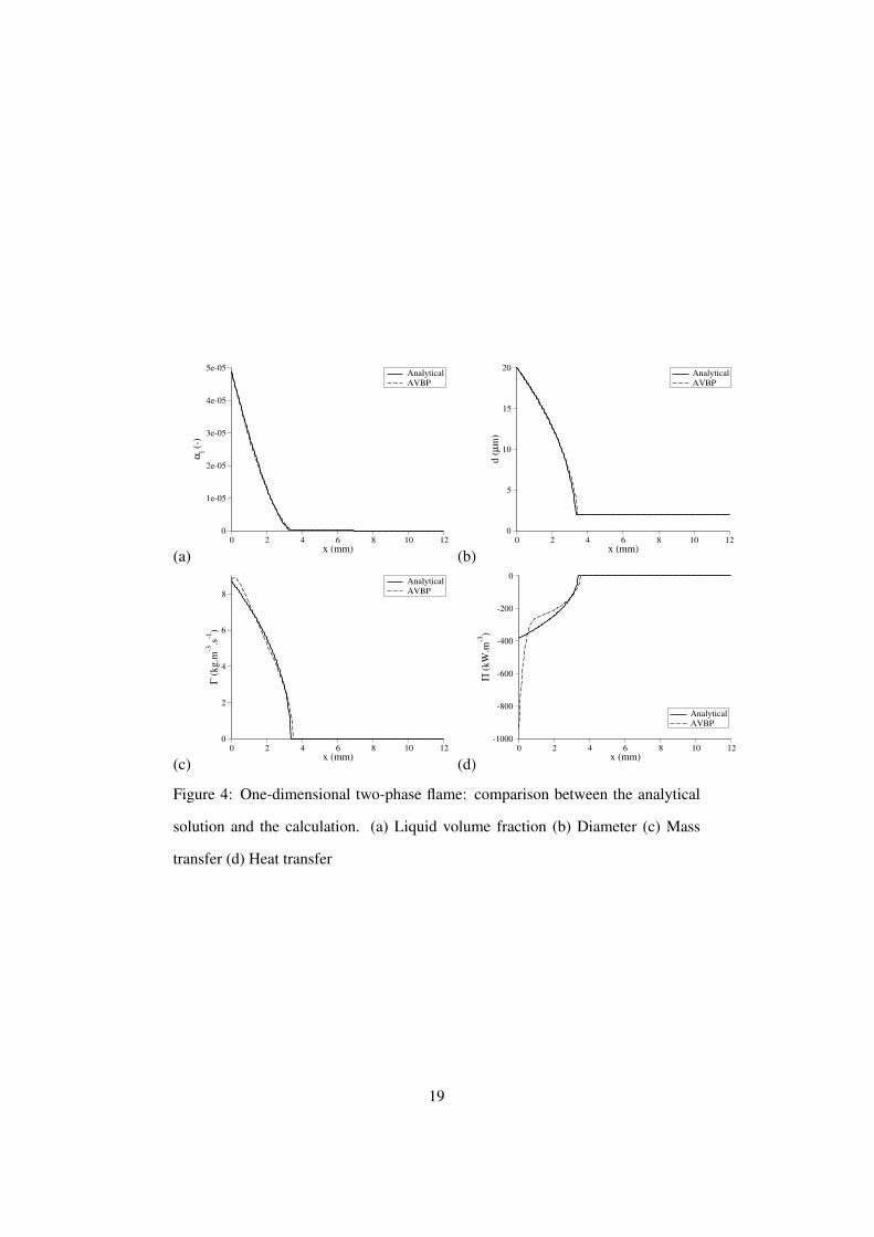
Fig. 3 and 4 show a comparison of the computed flame and the reference so- pages 18,19

lution for the liquid volume fraction and the droplet diameter, as well as mass and

heat exchange terms. The agreement between the two solutions is very good. Only

a slight difference is observed in the evaporation zone, as the reference solution is

calculated with a constant liquid temperature whereas a variable liquid temperature

17

is computed in the LES code.

(a)0.4 0.6 0.8 1.0 1.2 1.4 1.6

φ

0.00

0.25

0.50

0.75

1.00

1.25

1.50

S L (m.s-1

)

(b)0.4 0.6 0.8 1.0 1.2 1.4 1.6

φ

1600

1800

2000

2200

2400

2600

2800

T 2 (K)

Figure 2: Flame speed and maximum flame temperature obtained with the one-

step chemistry (lines) and compared with the reference complex chemistry curves

(circles).

(a)0 2 4 6 8 10 12

x (mm)

0

500

1000

1500

2000

T (

K)

AnalyticalAVBP

(b)0 2 4 6 8 10 12

x (mm)

0.00

0.05

0.10

0.15

0.20

0.25

Yk (-

)

AnalyticalJP10O2CO2H2O

Figure 3: One-dimensional two-phase flame: comparison between the analytical

solution and the calculation. (a) Gas temperature (b) Mass fractions.

18

(a)0 2 4 6 8 10 12

x (mm)

0

1e-05

2e-05

3e-05

4e-05

5e-05

α l (-)

AnalyticalAVBP

(b)0 2 4 6 8 10 12

x (mm)

0

5

10

15

20

d (µ

m)

AnalyticalAVBP

(c)0 2 4 6 8 10 12

x (mm)

0

2

4

6

8

Γ (k

g.m

-3.s-1

)

AnalyticalAVBP

(d)0 2 4 6 8 10 12

x (mm)

-1000

-800

-600

-400

-200

0

Π (k

W.m

-3)

AnalyticalAVBP

Figure 4: One-dimensional two-phase flame: comparison between the analytical

solution and the calculation. (a) Liquid volume fraction (b) Diameter (c) Mass

transfer (d) Heat transfer

19

4 Turbulent dispersion

A second validation is related to turbulent dispersion of the particles. Many ex-

periments on turbulent dispersion of particles are reported in the literature, but

only a few give enough detailed results to be used for comparison with LES and

validation of the numerical method [67–69]. In the present work the experiment

of Sommerfeld and Qiu [1] has been chosen as it is a well-known test case for

two-phase-flows and provides a significant amount of data. This configuration has

already been simulated with the EL approach on a refined mesh by Apte [70]. Our

objective is to evaluate the performance of the EE approach and the associated

models in the framework of LES with coarser grids.

The configuration (Fig. 5) is a simple pipe, with a swirling co-axial injection. see page 22

The Plexiglas tube is 1.5 m long with an inner diameter of 194 mm. Dust particles

are injected through the primary flow (inner pipe of the injector), with a mean di-

ameter of 45 µm and a size spectrum between 15-80 µm. The secondary annular

flow is swirled with a swirl number of 0.47 (calculated as the ratio of the axial

flux of angular momentum to the axial flux of linear momentum, integrated over

the injector section), resulting in a central annular recirculation zone. Particle size

and velocity as well as particle size-velocity correlations were measured at several

cross-sections using PDA. Although a polydisperse particle distribution was used

in the experiment, monodisperse results are available using size-conditioned aver-

ages. The Euler-Euler simulation is performed for particles of 45 µm and compared

to the same class of droplets used in the experiment. As for the dilute flows in gas

turbines, particle-particle interactions and two-way coupling are negligible in this

experiment so that statistics obtained for a single class can be compared to exper-

imental data. The corresponding Stokes number based on the particle relaxation

time and the flow time scale (outside the recirculation zone) is of the order of 2.2.

Sommerfeld and Qiu [1] define a second Stokes number that is more relevant to

20

Air flow

Mass flow rate of the primary jet (g/s) 9.9

Mass flow rate of the secondary jet (g/s) 38.3

Temperature (K) 300

Particles

Mass flow rate (g/s) 0.34

Mass loading 0.034

Temperature (K) 300

Size distribution (µm) 15-80

Table 2: Flow conditions for the Sommerfeld configuration.

the recirculation zone that leads to smaller values, of the order of 0.2 for particles

of 45 µm. Table 2 summarizes flow conditions and particle properties. see page 21

The simulation domain (Fig. 5) includes a portion of the inlet pipes (length see page 22

50 cm), the full test section and the stagnation chamber. The mesh (Fig. 5) contains see page 22

753,000 nodes, corresponding to 4,114,000 cells. It has a smallest cell size of

0.5 mm and is refined in the near-injector region. This leads to a CPU cost of

15 hours on a Compaq AlphaServer with 55 processors, for 40 ms of simulated

physical time. The simulation uses a Smagorinsky sub-grid scale model for the gas

and the model of Moreau [59] for the liquid. At the pipe inlet, fluctuating turbulent

velocities are prescribed on both the gas and the liquid phases [47] to reproduce

the inlet turbulence levels measured in the experiment.

Fig. 6 gives a global view of an instantaneous two-phase flow solution. The see page 22

opening of the jet is clearly visible as well as the recirculation zone for both phases.

After injection, the droplets travel first at the same velocity as the gas, but are

trapped by the recirculation zone around the stagnation region. In this zone the

21

Figure 5: Computational domain and mesh of the Sommerfeld configuration.

droplets accumulate and the number density increases strongly.

Figure 6: View of the instantaneous two-phase flow in the Sommerfeld configu-

ration: vertical plane: liquid axial velocity; horizontal plane: gas axial velocity;

isolines: droplet number density.

Figs. 7 and 8 show the gaseous mean velocity components (axial and tangen- see page 24

22

tial) and Figs. 9 and 10 show their RMS values, at different axial positions. The see page 25

agreement between the simulation results and the measurements is very good, for

both mean and fluctuating values, and up to the plane located furthest downstream.

In particular the location and thickness of the shear layer are well reproduced by

the simulation, both features that are known to be difficult to predict and demon-

strate the quality of the present calculation. The recirculation zone is also well

captured, at the correct location around 100 mm downstream the injector nozzle.

This is confirmed by the results on fluctuating velocities, showing that not only the

level but also the shape of the profiles are well captured.

The same velocity profiles are plotted for the liquid phase on Figs. 11 to 14. pages 26-27

Two experimental results are plotted, corresponding to either the data conditionned

on the single droplet size of 45 µm or to the data averaged on all droplet sizes.

Results show that the effect of polydispersion on the mean velocity is weak, except

near the stagnation zone induced by the recirculation where the polydispersion has

a tendency to delay the velocity decrease. As for the gas phase, the numerical

solution for the mean velocity is in good agreement with experimental data. The

main discrepancy is again near the stagnation zone, known to be difficult to predict,

and seems to indicate that the recirculation zone is too close from the injection

plane. However velocity profiles do not give a complete view of the flow structure

and the comparison between the numerical and experimental 3D flow fields (Fig. 6) see page 22

shows that the structures of the flow and of the recirculation zone are well captured

by the simulation. Compared to experiment, fluctuating velocity profiles are also

well captured in shape, but are underestimated by the simulation. This was also

observed in [47, 50] and is due to the missing RUM, that represents a significant

part of the particle sub-grid scale motion. Finally the liquid mass flow rate shown

on Fig. 15 indicates a correct numerical prediction of the liquid phase, with only a see page 28

reduced flux decrease along the axis due to the discrepancy between the velocities

23

0.10

0.09

0.08

0.07

0.06

0.05

0.04

0.03

0.02

0.01

0.00150

x=3mm

un velocity component LES EXPE

x10-3

150 x=25mm

x10-3

150 x=52mm

x10-3

150 x=85mm

x10-3

150 x=112mm

x10-3

150 x=155mm

x10-3

100 x=195mm

x10-3

100 x=315mm

Figure 7: Mean axial velocity profiles for the gas phase.

0.09

0.08

0.07

0.06

0.05

0.04

0.03

0.02

0.01

0.00150

x=3mm

ut velocity component LES EXPE

x10-3

150 x=25mm

x10-3

150 x=52mm

x10-3

150 x=85mm

x10-3

150 x=112mm

x10-3

150 x=155mm

x10-3

150 x=195mm

x10-3

150 x=315mm

Figure 8: Mean tangential velocity profiles for the gas phase.

already observed in the same region.

24

0.09

0.08

0.07

0.06

0.05

0.04

0.03

0.02

0.01

0.0050

x=3mm

un RMS velocity component LES EXPE

x10-3

50 x=25mm

x10-3

50 x=52mm

x10-3

50 x=85mm

x10-3

50 x=112mm

x10-3

50 x=155mm

x10-3

50 x=195mm

x10-3

50 x=315mm

Figure 9: RMS axial velocity profiles for the gas phase.

0.09

0.08

0.07

0.06

0.05

0.04

0.03

0.02

0.01

0.00420

x=3mm

ut RMS velocity component

x10-3

420 x=25mm

x10-3

420 x=52mm

x10-3

420 x=85mm

x10-3

420 x=112mm

x10-3

420 x=155mm

x10-3

420 x=195mm

x10-3

420 x=315mm

LES EXPE

Figure 10: RMS tangential velocity profiles for the gas phase.

25

0.09

0.08

0.07

0.06

0.05

0.04

0.03

0.02

0.01

0.00100

x=3mm

Un Liquid velocity component LES EXPE: polydispersed EXPE: 45 micron

100 x=25mm

100 x=52mm

100 x=85mm

100 x=112mm

100 x=155mm

100 x=195mm

100 x=315mm

Figure 11: Mean axial velocity profiles for the liquid phase. Numerical simulations

use 45 µm monodisperse droplets.

0.09

0.08

0.07

0.06

0.05

0.04

0.03

0.02

0.01

0.00840

x=3mm 840

x=25mm 840

x=52mm 840

x=85mm 840

x=112mm 840

x=155mm 840

x=195mm840

x=315mm

Ut Liquid velocity component LES EXPE: polydispersed EXPE: 45 micron

Figure 12: Mean tangential velocity profiles for the liquid phase. Numerical simu-

lations use 45 µm monodisperse droplets.

26

0.09

0.08

0.07

0.06

0.05

0.04

0.03

0.02

0.01

0.00420 420 420 420 420 420 420 420

x=3mm

Un Liquid RMS velocity component

x=25mm x=52mm x=85mm x=112mm x=155mm x=195mm x=315mm

LES EXPE: polydispersed EXPE: 45 micron

Figure 13: RMS axial velocity profiles for the liquid phase. Numerical simulations

use 45 µm monodisperse droplets.

0.09

0.08

0.07

0.06

0.05

0.04

0.03

0.02

0.01

0.001.50

x10-3

1.50

x10-3

1.50

x10-3

1.50

x10-3

1.50

x10-3

1.50

x10-3

1.50

x10-3

1.50 x=3mm

Ut Liquid RMS velocity component

x=25mm x=52mm x=85mm x=112mm x=155mm x=195mm x=315mm

LES EXPE: polydispersed EXPE: 45 micron

Figure 14: RMS tangential velocity profiles for the liquid phase. Numerical simu-

lations use 45 µm monodisperse droplets.

27

0.09

0.08

0.07

0.06

0.05

0.04

0.03

0.02

0.01

0.000.40.0

x=3mm

x10-3

0.40.0 x=25mm

x10-3

0.40.0 x=52mm

x10-3

0.40.0 x=85mm

x10-3

0.40.0 x=112mm

x10-3

0.40.0 x=155mm

x10-3

0.40.0 x=195mm

x10-3

0.40.0 x=315mm

Axial Flux LES EXPE: polydispersed

Figure 15: Axial liquid mass flux. Numerical simulations use 45 µm monodisperse

droplets.

28

5 Reacting flow in an aircraft combustion chamber

5.1 Configuration

The last test case is a 3D sector of 22.5-degrees of an annular combustor at atmo-

spheric pressure. The kerosene Liquid Spray (LS) is located at the center of the

main Swirled Inlet (SI) (Fig. 17). Small Holes (H), located around the inlet aim at see page 31

lifting the flame and protect the injector from high temperatures. The perforations

localized on the upper and lower walls are divided in two parts. The Primary Jets

(PJ) bring cold air to the flame in the first part of the combustor where combustion

takes place. The Dilution Jets (DJ) inject air further downstream to reduce and

homogenise the outlet temperature to protect the turbine. The Spark Plug (SP) is

located under the upper wall between two (PJ) (Fig. 18). The geometry (Fig. 19) see page 31

also includes cooling films which protect walls from the flame. see page 31

The inlet and outlet boundary conditions use characteristic treatments with re-

laxation coefficients to reduce acoustic reflexion [10,71]. The SI imposed velocity

field mimics the swirler influence. Figure 16 displays profiles of the three compo- see page 31

nents of the air velocity as prescribed along the axis of the spray (AB on Fig. 19) see page 31

in reduced units: u∗ = u/U0 as a function of r∗ = r/R0 where U0 is the bulk

velocity and R0 is the radius of the SI. The other inlets are simple jets. The in-

jected spray is monodisperse, composed of droplets of diameter of 15 µm leading

to a Stokes number, based on the droplet relaxation time and the swirl flow time of

0.57. The volume fraction, αl ' 10−3, is imposed for a disk of radius r∗ = 0.4.

This corresponds to a lean global stoichiometric ratio of 0.28. At injection, the liq-

uid velocity is equal to the gaseous velocity as the droplet Stokes number is lower

than one. The droplet inlet temperature equals 288 K and the air is at 525 K. No-

slip conditions are used on the upper and lower walls while a symmetry condition

29

Air flow

Total mass flow rate (g/s) 119

Temperature (K) 525

Pressure (bar) 1

Liquid fuel

Mass flow rate (g/s) 2.38

Temperature (K) 300

Droplet size (µm) 15

Table 3: Flow conditions for the gas turbine configuration.

is used on the sector sides. All conditions are summarized in Table 3. see page 30

The unstructured mesh is composed of 400,000 nodes and 2,300,000 tetrahe-

dra, which is typical and reasonable for LES of such configuration. The explicit

time step is ∆t ' 0.22 µs. The mesh is refined close to the inlets and in the com-

bustion zone (Fig. 20), leading to a flame thickening factor of the order of 10. The see page 31

one-step chemical scheme described in section 3 is used here without any changes.

It has been checked that in the simulation the flame mostly burns mixtures with an

equivalence ratio in the range between 0.5 and 1, where the chemical scheme is

valid.

5.2 Steady spray flame

First a steady turbulent two-phase flame is calculated. The 15 µm droplet mo-

tion follows the carrier phase dynamics so that the Centered Recirculation Zones

(CRZ) are similar for gas and liquid, as illustrated on Fig. 21, showing the in- see page 32

stantaneous backflow lines of both phases, plotted in the vertical central cutting

30

1.00

0.90

0.80

0.70

0.60

0.50

0.40

0.30

0.20

0.10

0.002.01.00.0

u*

un*

ur*

ut*

r*

Figure 16: Normal, radial and tangential injection velocity profiles for the burner

configuration: r∗ = r/R0 and u∗ = u/U0 where R0 and U0 are respectively the

SI radius and the bulk velocity.

LSPJ DJSI

H

Figure 17: Geometry sketch : side view

SP

Figure 18: Geometry sketch : top view

Figure 19: Chamber geometry Figure 20: Mesh view on central plane

plane. Maintained by this CRZ, the droplets accumulate and the droplet number

density, presented with the liquid volume fraction field on Fig. 21, rises above its see page 32

31

initial value: a zone where the droplet number density nl is larger than 2nl,inj

(where nl,inj is its value at injection) is formed downstream of the injector at a dis-

tance approximately half of the nozzle diameter (lines with circles on Fig 21). The see page 32

increased residence time of these droplets, whose diameter field is presented on

Fig. 22, increases the local equivalence ratio distribution. The heat transfer linked see page 32

to the phase change leads to the reduction of the gaseous temperature, as shown

by the isoline T = 450 K on Fig. 23, and an increase of the dispersed phase tem- see page 34

perature. Thus, the CRZ, by trapping evaporating droplets, stabilises the vaporised

fuel and the flame. The flame front visualized on Fig. 23 by the heat release field see page 34

Figure 21: Instantaneous field of volume

fraction in the central cutting plane of

the chamber, with zero-velocity lines and

nl = 2ninj isoline.

Figure 22: Instantaneous field of droplet

diameter in the central cutting plane of

the chamber, with equivalence ratio iso-

lines for the values 1 and 10.

is influenced by both flow dynamics and evaporation rate. The main phenomena

controlling flame stabilisation are :

1. the air velocity must be low enough to match the turbulent flame velocity :

32

the dynamics of the carrier phase (and in particular the CRZ) stabilises the

flame front on a stable pocket of hot gases

2. zones where the local mixture fraction is within flammability limits must

exist : combustion occurs between the fuel vapour radially dispersed by the

swirl and the ambient air, where the equivalence ratio is low enough

3. the heat release must be high enough to maintain evaporation and reaction :

the sum of heat flux Π and heat release ωT , plotted on Fig. 23, allows to iden- see page 34

tify the zone ( ) where the heat transfer due to evaporation compensates

the local heat release : Π + ωT = 0.

In the present case, the flame front is stabilised by the CRZ (1) but the heat release

magnitude is reduced in the evaporation zone because of both effects (2) and (3).

To determine the flame regime (premixed and/or diffusion), the Takeno index T =

∇YF .∇YO and an indexed reaction rate ω∗F = ωF

T|∇YF |.|∇YO| are used [72]. The

flame structure is then divided into two parts : ω∗F = +ωF in the premixed regime

and ω∗F = −ωF in the diffusion regime (Fig. 24). In the primary zone, the partially see page 34

premixed regime dominates because of the unsteady inhomogeneous fuel vapour.

In the dilution zone, the unburned fuel reacts with dilution jets through a diffusion

flame, as confirmed by the coincidence between the flame and the stoichiometric

line.

In his review on vortex breakdown, Lucca-Negro [73] classifies the hydrody-

namic instabilities appearing in swirled flows. For high swirl numbers, the axial

vortex breaks down at the stagnation point S and a spiral is created around a central

recirculation zone CRZ (Fig. 25) : this vortex breakdown is the so-called Precess- see page 34

ing Vortex Core (PVC) and occurs in a large number of combustors [74]. LES cap-

tures the vortex breakdown in the combustor and its frequency is evaluated with the

backflow line on a transverse plane (Fig. 26) at six successive times marked with see page 34

33

Figure 23: Flame front

Figure 24: Flame structure visualized by

the indexed reaction rate. Black zones

correspond to premixed flames and white

zones to diffusion flames.

a number from 1 to 6 and separated by 0.5 ms. The turnover time is estimated at

τPV C ' 3.5 ms, corresponding to a frequency of fPV C ' 290 Hz. Moreover, the

three rotating motions of the SI, the whole PVC structure and the spiral winding

turn in the same direction, as illustrated by the rotating arrows on Fig. 25. The PVC see page 34

defined on Fig. 27a controls the motions of both the Vaporised Fuel (VF) zone and see page 35

the flame front. Fig. 27b displays the temperature field, the maximum fuel mass see page 35

fraction (white lines) and the flame front (black isolines of reaction rate ωF ). In

the cutting plane, defined on Fig. 27a, the CRZ stabilises hot gases and enhances see page 35

evaporation leading to a cold annular zone where the maximum fuel mass fraction

precesses. The flame motion follows the PVC and the reaction rate is driven by the

fuel vapour concentration.

34

CRZ

PVC

S

SI

Figure 25: Precessing Vortex Core.Figure 26: Backflow line : transverse cut

in plane P1 (Fig 19).

a.

SI

b.

VF

Flame

b.

Figure 27: PVC influence on evaporation and combustion (left). Fields of temper-

ature and isolines of fuel vapor (white lines) and reaction rate (black lines) (right).

5.3 Ignition sequence

Ignition sequences can also be simulated with the same LES tool. The numerical

method used to mimic an ignition by spark plug in the combustion chamber is

the addition of the source term ωspark in Eq. (23). This source term, defined by

Eq. (23), is a gaussian function located at (x0, y0, z0) near the upper wall between

both primary jets and deposited at time t = t0 = 0. The spark duration, typical of

industrial spark plugs, is σt = 0.04 ms. The total deposited energy is Espark =

35

150 J .

ωspark =Espark

(2π)2σtσr3e− 1

2

[(t−t0

σt

)2

+(

x−x0σr

)2+(

y−y0σr

)2+(

z−z0σr

)2

](23)

The temporal evolution of the total (i.e. spatially integrated) power deposited by

the spark is presented on Fig. 28, along with the total heat release ωT and the see page 36

spatially averaged temperature. After a heating phase due to the source term on

the energy equation (up to approximately 0.08 ms), the temperature is sufficient to

initiate the reaction between fuel vapour and air, leading to a sudden increase of the

heat release of the exothermic reaction. When the spark is stopped (at≈ 0.18 ms),

the total heat release decreases, and finally stabilizes at a level corresponding to a

propagating flame, while the mean temperature continues to increase: the ignition

is successful.

0.0 0.1 0.2 0.3 0.4 0.5 0.6 0.7Time (ms)

0

400

800

1200

1600

Inte

gral

pow

er (

kW)

Spark powerCombustion heat release

500

600

700

800

Tem

pera

ture

(K

)Mean temperature

Figure 28: Total (spatially integrated) source term ωspark, total heat release ωT ,

and spatially averaged temperature.

36

The transition from the ignition of the first flame kernel (t = 0.2 ms) to a

complete stabilisation takes more time (more than 3 ms) and is illustrated on the

longitudinal central cutting plane identified in Fig. 29 with the fuel mass fraction see page 39

field and the reaction rate isolines. The first image is presented at t = 0.2 ms

and after, successive images are separated by ∆t = 0.2 ms. At the beginning of

the computation, the 15 µm droplets evaporate in the ambient air at T = 525 K

creating a turbulent cloud of vaporised fuel in the whole primary zone. This fuel

vapour is trapped by the CRZ and is transported from the evaporation zone to the

spark plug area. At t = 0, the spark ignition leads to the creation of a hot kernel.

The propagation of the flame front created by this pocket of hot gases is highly

controlled by the fuel vapour distribution between t = 0 and t = 1 ms. After

t = 0.2 ms, this flame loses its spherical shape due to convective effects. The

downstream side of the flame front is blown away and extinguishes by lack of fuel

while the bottom side is progressing towards the center line where the fuel vapour

concentration is high. When entering the CRZ (t = 1 ms), the front is strongly

wrinkled by the large turbulent scales of the flow. However, in the upstream region

of the CRZ, the low velocities enable to stabilize the edge of the reacting zone

close to the fuel injection (t = 1 to 1.4 ms). In this region, the flame and the back-

flow maintain a high temperature ambiant leading to a strong evaporation rate and

creating a stable fuel vapour concentrated spot (t = 1.6 to 2.4 ms). Due to the

swirled jet, this fuel vapour is radially dispersed into the air flow and produce a

flammable mixture. Burning this mixture, the flame is able to spread in the radial

direction and finally occupies a large section of the primary zone (t = 2.4 ms).

This last topology corresponds to the steady spray flame described in the previous

section.

This ignition sequence shows the important role of the liquid phase, respon-

sible for the great differences with the ignition of a purely gaseous flame. The

37

controlling mechanism is evaporation, that delays the start of the chemical reaction

and, together with the droplet turbulent dispersion, modifies the fuel vapor distri-

bution and consequently the flame front propagation. This was never visualized

and, despite the use of simplified models, the simulation provides a good and new

qualitative description of the phenomena.

38

0.2 ms 0.4 ms 0.6 ms 0.8 ms

1.0 ms 1.2 ms 1.4 ms 1.6 ms

1.8 ms 2.0 ms 2.2 ms 2.4 ms

Figure 29: Flame front propagation on fuel mass fraction field (white: 0 → black:

0.35)

39

6 Conclusions

A steady spray flame in a realistic aeronautical combustor has been computed us-

ing a parallel LES Euler/Euler solver. This approach was first tested in two simple

reference cases: a one-dimensional laminar two-phase flame of JP10 with air and

a swirled non-reacting flow with solid particles [1]. The influence of the dispersed

phase on the flame motion has been highlighted, in particular the role of the evapo-

ration process. The unsteady approach brings new insight into the physics of such

complex reactive two-phase flows. Furthermore, it allows the computation of an

ignition sequence from the formation of the first spherical flame front to the sta-

bilisation of the turbulent spray flame. Obviously more quantitative comparisons

of the present method with existing Euler-Lagrange methods and with experiments

(such as [47]) are needed. But this paper shows that despite its limitations and

still open modelling issues, the Euler-Euler approach already leads to interesting

results on the tested configurations and demontrates its feasability and capabilities

for two-phase flow combustion.

Acknowledgements-This work was supported by the Safran group. The two moni-

tors Dr. C. Berat and Dr. M. Cazalens are gratefully acknowledged.

40

References

[1] M. Sommerfeld and H. H. Qiu. Characterisation of particle-laden, confined

swirling flows by phase-doppler anemometry ad numerical calculation. Int.

J. Multiphase Flow, 19(6):1093–1127, 1993.

[2] D. Caraeni, C. Bergstrom, and L. Fuchs. Modeling of liquid fuel injection,

evaporation and mixing in a gas turbine burner using large eddy simulation.

Flow Turb. and Combustion , 65:223–244, 2000.

[3] V.K. Chakravarthy and S. Menon. Subgrid modeling of turbulent premixed

flames in the flamelet regime. Flow Turb. and Combustion , 65:133–161,

2000.

[4] O. Colin, F. Ducros, D. Veynante, and T. Poinsot. A thickened flame model

for large eddy simulations of turbulent premixed combustion. Phys. Fluids ,

12(7):1843–1863, 2000.

[5] H. Forkel and J. Janicka. Large-eddy simulation of a turbulent hydrogen

diffusion flame. Flow Turb. and Combustion , 65(2):163–175, 2000.

[6] H. Pitsch and L. Duchamp de la Geneste. Large eddy simulation of premixed

turbulent combustion using a level-set approach. Proc of the Comb. Institute,

29:2001–2005, 2002.

[7] K. Mahesh, G. Constantinescu, and P. Moin. A numerical method for large-

eddy simulation in complex geometries.

[8] L. Selle, G. Lartigue, T. Poinsot, R. Koch, K.-U. Schildmacher, W. Krebs,

B. Prade, P. Kaufmann, and D. Veynante. Compressible large-eddy simula-

tion of turbulent combustion in complex geometry on unstructured meshes.

Combust. Flame , 137(4):489–505, 2004.

41

[9] Y. Sommerer, D. Galley, T. Poinsot, S. Ducruix, F. Lacas, and D. Veynante.

Large eddy simulation and experimental study of flashback and blow-off in a

lean partially premixed swirled burner. J. of Turbulence, 5, 2004.

[10] V. Moureau, G. Lartigue, Y. Sommerer, C. Angelberger, O. Colin, and

T. Poinsot. High-order methods for DNS and LES of compressible multi-

component reacting flows on fixed and moving grids. J. Comput. Phys. ,

202(2):710–736, 2005.

[11] S. Roux, G. Lartigue, T. Poinsot, U. Meier, and C. Berat. Studies of mean and

unsteady flow in a swirled combustor using experiments, acoustic analysis

and large eddy simulations. Combust. Flame , 141:40–54, 2005.

[12] T. Poinsot and D. Veynante. Theoretical and numerical combustion. R.T.

Edwards, 2nd edition., 2005.

[13] A.H. Lefebvre. Gas Turbines Combustion. Taylor & Francis, 1999.

[14] C. Weber and Z. Angrew. The decomposition of a liquid jet. Math. Mech.,

11:136–154, 1931.

[15] S. Nukiyama and Y. Tanasawa. Experiments in on the atomization of liquids

in air stream. report 3 : on the droplet-size distribution in an atomized jet.

Trans. Soc. Mech. Eng. Japan, 5:62–67, 1939.

[16] R. D. Reitz and F. V. Bracco. Mechanism of atomization of a liquid jet.

Physics of Fluids, 25(10):1730–1742, 1982.

[17] Z. Han, S. Parrish, P.V. Farrell, and D. Reitz. Modeling atomization processes

of pressure-swirl hollow-cone fuel sprays. Atomization and Sprays, (6):663–

684, 1997.

42

[18] J.C. Lasheras and E.J. Hopfinger. Liquid jet instability and atomisation in a

coaxial gas stream. Ann. Rev. Fluid. Mech., 32:275–308, 2000.

[19] S.V. Apte, K. Mahesh, P. Moin, and J.C. Oefelein. Large-eddy simulation of

swirling particle-laden flow in a coaxial combustor. International Journal of

Multiphase Flow, 29:1311–1331, 2003.

[20] V.M. Alipchenkov and L.I. Zaichik. Modeling of the turbulent motion of

particles in a vertical channel. Journal of Fluid Dynamics, 41(4):531–544,

2006.

[21] M. Boivin, K. Squires, and O. Simonin. On the prediction of gas-solid flows

with two-way coupling using large eddy simulation. Phys. Fluids , 12(8),

2000.

[22] B. Oesterle and L.I. Zaichik. On lagrangian time scales and particle dis-

persion modeling in equilibrium turbulent shear flows. Physics of Fluids,

16(9):3374–3384, 2004.

[23] C. Marchioli, M. Picciotto, and A. Soldati. Particle dispersion and wall-

dependent turbulent flow scales: implications for local equilibrium models.

Journal of Turbulence, 7(60):1–12, 2006.

[24] M. Benson, T. Tanaka, and J.K. Eaton. Effects of wall roughness on par-

ticle velocities in a turbulent channel flow. Journal of Fluids Engineering,

127(2):250–256, 2005.

[25] M. Sommerfeld and J. Kussin. Analysis of collision effects for turbulent

gas-particle flow in a horizontal channel. Part (ii). integral properties and val-

idation. International Journal of Multiphase Flow, 29(4):701–718, 2003.

43

[26] I. Gokalp, C. Chauveau, C. Morin, B. Vieille, and M. Birouk. Improving

dropelt breakup and vapoization models by including high pressure and tur-

bulence effects. Atomiztion and Sprays, 10:475–510, 2000.

[27] V. Sankaran and S. Menon. Les of spray combustion in swirling flows. J. of

Turbulence, 3:011, 2002.

[28] K. Mahesh, G. Constantinescu, S. Apte, G. Iaccarino, F. Ham, and P. Moin.

Progress towards large-eddy simulation of turbulent reacting and non-

reacting flows in complex geometries. In Annual Research Briefs, pages 115–

142. Center for Turbulence Research, NASA Ames/Stanford Univ., 2002.

[29] S. V. Apte, M. Gorokhovski, and P. Moin. Large-eddy simulation of atom-

izing spray with stochastic modeling of secondary breakup. In ASME Turbo

Expo 2003 - Power for Land, Sea and Air, Atlanta, Georgia, USA, 2003.

[30] F. Ham, S. V. Apte, G. Iaccarino, X. Wu, M. Herrmann, G. Constantinescu,

K. Mahesh, and P. Moin. Unstructured les of reacting multiphase flows in

realistic gas turbine combustors. In Annual Research Briefs. Center for Tur-

bulence Research, 2003.

[31] H. Enwald, E. Peirano, and A.-E. Almstedt. Eulerian two-phase flow theory

applied to fluidization. Int. J. Multiphase Flow, 22:21–66, 1996.

[32] E. Peirano and B. Leckner. Fundamentals of turbulent gas-solid flows applied

to circulating fluidized bed combustion. Prog. Energy Comb. Sci. , 24:259–

296, 1998.

[33] J. Gao, C. Xu, S. Lin, and G. Yang. Simulations of gas-liquid-solid 3-phase

flow and reaction in FCC riser reactors. AIChE Journal, 47(3):677–692,

2001.

44

[34] A.K. Das. Computational fluid dynamics simulation of gas-solid risers : re-

active flow modelling. PhD thesis, Universiteit Gent, 2002.

[35] A. Gobin, H. Neau, O. Simonin, J.-R. Linas, V. Reiling, and J.-L. Selo. Fluid

dynamic numerical simulation of a gas phase polymerization reactor. Int. J.

of Numerical Methods in Fluids, 43:1199–1220, 2003.

[36] P. Moin. Large eddy simulation of multi-phase turbulent flows in realistic

combustors. Prog. in Computational Fluid Dynamics, 4:237–240, 2004.

[37] A Kaufmann. Vers la simulation des grandes echelles en formulation Eu-

ler/Euler des ecoulements reactifs diphasiques. PhD thesis, INPT, 2004.

[38] P. Fevrier, O. Simonin, and K. Squires. Partitioning of particle velocities in

gas-solid turbulent flows into a continuous field and a spatially uncorrelated

random distribution: Theoretical formalism and numerical study. J. Fluid

Mech., 533:1–46, 2005.

[39] J.B. Mossa. Extension polydisperse pour la description Euler/Euler des

ecoulements diphasiques reactifs. PhD thesis, INP Toulouse, 2005.

[40] E. Riber. Developpement de la methode de simulation aux grandes echelles

pour les ecoulements diphasiques turbulents. PhD thesis, INP Toulouse,

2007.

[41] P. Fede and O. Simonin. Numerical study of the subgrid fluid turbulence ef-

fects on the statistics of heavy colliding particles. Phys. Fluids , 18(045103),

2006.

[42] P. Fede, P. Villedieu, O. Simonin, and K.D. Squires. Stochastic modeling of

the subgrid fluid velocity fluctuations seen by inertial particles. In Proc of the

Summer Program. Center for Turbulence Research, NASA Ames/Stanford

Univ., 2006.

45

[43] M. Moreau, B. Bedat, and O. Simonin. From euler-lagrange to euler-euler

large eddy simulation approaches for gas-particle turbulent flows. In ASME

Fluids Engineering Summer Conference. ASME FED, 2005.

[44] E. Riber, M. Moreau, O. Simonin, and B. Cuenot. Towards large eddy simula-

tion of non-homogeneous particle laden turbulent gas flows using euler-euler

approach. In 11th Workshop on Two-Phase Flow Predictions, Merseburg,

Germany, 2005.

[45] O.A. Druzhinin and S. Elghobashi. On the decay rate of isotropic turbulence

laden with microparticles. Phys. Fluids , 11(3), 1999.

[46] S. Chapman and T.G. Cowling. The Mathematical Theory of Non-Uniform

Gases. Cambridge University Press, cambridge mathematical library edition,

1939 (digital reprint 1999).

[47] E. Riber, M. Garcıa, V. Moureau, H. Pitsch, O. Simonin, and T. Poinsot. Eval-

uation of numerical strategies for LES of two-phase reacting flows. In CTR

Summer Program, Center for Turbulence Research, NASA AMES, Stanford

University, USA, 2006.

[48] D.B. Spalding. The combustion of liquid fuels. In 4th Symp. (Int.) on Com-

bustion. The Combustion Institute, Pittsburgh, 1953.

[49] A. Kaufmann, O. Simonin, T. Poinsot, and J. Helie. Dynamics and dis-

persion in eulerian-eulerian DNS of two phase flow. In Proceeding of the

Summer Program, pages 381–391, Center for Turbulence Research, NASA

AMES/Stanford University, USA, 2002.

[50] E. Riber, M. Moreau, O. Simonin, and B. Cuenot. Development of Euler-

Euler LES approach for gas-particle turbulent jet flow. In ASME - European

Fluids Enigneering Summer Meeting, 2006.

46

[51] F. Nicoud and F. Ducros. Subgrid-scale stress modelling based on the square

of the velocity gradient. Flow Turb. and Combustion , 62(3):183–200, 1999.

[52] J.-Ph. Legier, T. Poinsot, and D. Veynante. Dynamically thickened flame

large eddy simulation model for premixed and non-premixed turbulent com-

bustion. In Summer Program 2000, pages 157–168, Center for Turbulence

Research, Stanford, USA, 2000.

[53] C. Martin, L. Benoit, Y. Sommerer, F. Nicoud, and T. Poinsot. Les and acous-

tic analysis of combustion instability in a staged turbulent swirled combustor.

AIAA Journal , 44(4):741–750, 2006.

[54] P. Schmitt, T.J. Poinsot, B. Schuermans, and K. Geigle. Large-eddy sim-

ulation and experimental study of heat transfer, nitric oxide emissions and

combustion instability in a swirled turbulent high pressure burner.

[55] A. Sengissen, A. Giauque, G. Staffelbach, M. Porta, W. Krebs, P. Kaufmann,

and T. Poinsot. Large eddy simulation of piloting effects on turbulent swirling

flames. In Proc. of the Combustion Institute, 31, 2007.

[56] P. Moin, K. Squires, W. Cabot, and S. Lee. A dynamic subgrid-scale

model for compressible turbulence and scalar transport. Phys. Fluids , A

3(11):2746–2757, 1991.

[57] B. Vreman, B. Geurts, and H. Kuerten. Subgrid modeling in LES of com-

pressible flow. Appl. Sci. Res., 54:191–203, 1995.

[58] A. Yoshizawa. Statistical theory for compressible turbulent shear flows, with

the application to subgrid modeling. Phys. Fluids , 29(7):2152–2164, 1986.

[59] M. Moreau, B. Bedat, and O. Simonin. A priori testing of subgrid stress

models for euler-euler two-phase LES from euler-lagrange simulations of

47

gas-particle turbulent flow. In 18th Ann. Conf. on Liquid Atomization and

Spray Systems. ILASS Americas, 2005.

[60] C. Hirsch. Numerical Computation of internal and external flows. John Wi-

ley, New York, 1988.

[61] O. Colin and M. Rudgyard. Development of high-order Taylor-Galerkin

schemes for unsteady calculations. J. Comput. Phys. , 162(2):338–371, 2000.

[62] T. Poinsot and S. Lele. Boundary conditions for direct simulations of com-

pressible viscous flows. J. Comput. Phys. , 101(1):104–129, 1992.

[63] T. H. Lin, C. K. Law, and S. H. Chung. Theory of laminar flame propaga-

tion in off-stoichiometric dilute sprays. Int. J. of Heat and Mass transfer,

31:1023–1034, 1988.

[64] T. H. Lin and Y. Y. Sheu. Theory of laminar flame propagation in near-

stoichiometric dilute sprays. Int. J. of Heat and Mass transfer, 84:333–342,

1991.

[65] C. Martin. Eporck user guide v1.8. Technical report, CERFACS, 2004.

[66] S.C. Li, B. Varatharajan, and F.A. Williams. Chemistry of jp-10 ignition.

AIAA Journal, 39(12):2351–2356, 2001.

[67] K. Hishida, K. Takemoto, and M. Maeda. Turbulent characteristics of gas-

solids two-phase confined jet. Japanese Journal of Multiphase Flow, 1(1):56–

69, 1987.

[68] K. Squires and J. Eaton. Measurements of particle dispersion obtained from

direct numerical simulations of isotropic turbulence. J. Fluid Mech. , 226:1–

35, 1991.

48

[69] J. S. Vames and T. J. Hanratty. Turbulent dispersion of droplets for air flow

in a pipe. Experiments in Fluids, 6(2):94–104, 2004.

[70] S. V. Apte, K. Mahesh, and T. Lundgren. A eulerian-lagrangian model to

simulate two-phase/particulate flows. In Annual Research Briefs. Center for

Turbulence Research, 2003.

[71] L. Selle, F. Nicoud, and T. Poinsot. The actual impedance of non-reflecting

boundary conditions: implications for the computation of resonators. AIAA

Journal , 42(5):958–964, 2004.

[72] H. Yamashita, M. Shimada, and T Takeno. A numerical study on flame sta-

bility at the transition point of jet diffusion flame. In 26th Symp. (Int.) on

Combustion, pages 27 – 34. The Combustion Institute, Pittsburgh, 1996.

[73] O. Lucca-Negro and T. O’Doherty. Vortex breakdown: a review. Prog.

Energy Comb. Sci. , 27:431–481, 2001.

[74] L. Selle. Simulation aux grandes echelles des couplages acoustique / com-

bustion dans les turbines a gaz. Phd thesis, INP Toulouse, 2004.

List of Figures

1 Sketch of the 1D-flame test case: top - homogeneous flame, bottom

- heterogeneous flame. . . . . . . . . . . . . . . . . . . . . . . . 17

2 Flame speed and maximum flame temperature obtained with the

one-step chemistry (lines) and compared with the reference com-

plex chemistry curves (circles). . . . . . . . . . . . . . . . . . . . 18

3 One-dimensional two-phase flame: comparison between the ana-

lytical solution and the calculation. (a) Gas temperature (b) Mass

fractions. . . . . . . . . . . . . . . . . . . . . . . . . . . . . . . 18

49

4 One-dimensional two-phase flame: comparison between the ana-

lytical solution and the calculation. (a) Liquid volume fraction (b)

Diameter (c) Mass transfer (d) Heat transfer . . . . . . . . . . . . 19

5 Computational domain and mesh of the Sommerfeld configuration. 22

6 View of the instantaneous two-phase flow in the Sommerfeld con-

figuration: vertical plane: liquid axial velocity; horizontal plane:

gas axial velocity; isolines: droplet number density. . . . . . . . . 22

7 Mean axial velocity profiles for the gas phase. . . . . . . . . . . . 24

8 Mean tangential velocity profiles for the gas phase. . . . . . . . . 24

9 RMS axial velocity profiles for the gas phase. . . . . . . . . . . . 25

10 RMS tangential velocity profiles for the gas phase. . . . . . . . . 25

11 Mean axial velocity profiles for the liquid phase. Numerical simu-

lations use 45 µm monodisperse droplets. . . . . . . . . . . . . . 26

12 Mean tangential velocity profiles for the liquid phase. Numerical

simulations use 45 µm monodisperse droplets. . . . . . . . . . . 26

13 RMS axial velocity profiles for the liquid phase. Numerical simu-

lations use 45 µm monodisperse droplets. . . . . . . . . . . . . . 27

14 RMS tangential velocity profiles for the liquid phase. Numerical

simulations use 45 µm monodisperse droplets. . . . . . . . . . . 27

15 Axial liquid mass flux. Numerical simulations use 45 µm monodis-

perse droplets. . . . . . . . . . . . . . . . . . . . . . . . . . . . . 28

16 Normal, radial and tangential injection velocity profiles for the

burner configuration: r∗ = r/R0 and u∗ = u/U0 where R0 and

U0 are respectively the SI radius and the bulk velocity. . . . . . . 31

17 Geometry sketch : side view . . . . . . . . . . . . . . . . . . . . 31

18 Geometry sketch : top view . . . . . . . . . . . . . . . . . . . . . 31

19 Chamber geometry . . . . . . . . . . . . . . . . . . . . . . . . . 31

50

20 Mesh view on central plane . . . . . . . . . . . . . . . . . . . . . 31

21 Instantaneous field of volume fraction in the central cutting plane

of the chamber, with zero-velocity lines and nl = 2ninj isoline. . 32

22 Instantaneous field of droplet diameter in the central cutting plane

of the chamber, with equivalence ratio isolines for the values 1 and

10. . . . . . . . . . . . . . . . . . . . . . . . . . . . . . . . . . . 32

23 Flame front . . . . . . . . . . . . . . . . . . . . . . . . . . . . . 34

24 Flame structure visualized by the indexed reaction rate. Black

zones correspond to premixed flames and white zones to diffusion

flames. . . . . . . . . . . . . . . . . . . . . . . . . . . . . . . . . 34

25 Precessing Vortex Core. . . . . . . . . . . . . . . . . . . . . . . . 35

26 Backflow line : transverse cut in plane P1 (Fig 19). . . . . . . . . 35

27 PVC influence on evaporation and combustion (left). Fields of

temperature and isolines of fuel vapor (white lines) and reaction

rate (black lines) (right). . . . . . . . . . . . . . . . . . . . . . . 35

28 Total (spatially integrated) source term ωspark, total heat release

ωT , and spatially averaged temperature. . . . . . . . . . . . . . . 36

29 Flame front propagation on fuel mass fraction field (white: 0 →

black: 0.35) . . . . . . . . . . . . . . . . . . . . . . . . . . . . . 39

List of Tables

1 Set of (6+N) conservation equations, where N is the number of

chemical species. . . . . . . . . . . . . . . . . . . . . . . . . . . 15

2 Flow conditions for the Sommerfeld configuration. . . . . . . . . 21

3 Flow conditions for the gas turbine configuration. . . . . . . . . . 30

51