CEAA-2010: 22-25 September, Svetlogorsk, Russia

Delayed DetachedDelayed Detached--Eddy SimulationEddy Simulation of Tandem Cylindersof Tandem Cylinders

A. Garbaruk, M. Shur, M. Strelets NTS, SPbSPU P. R. Spalart

Boeing Commercial Airplanes

and R. Balakrishnan

Argonne National LaboratoryEmail: strelets@mail.rcom.ru

OutlineOutline

• Preliminary Comments• Flow Conditions• Simulation Approach and Numerical Method• Grids• Results• Conclusions

2

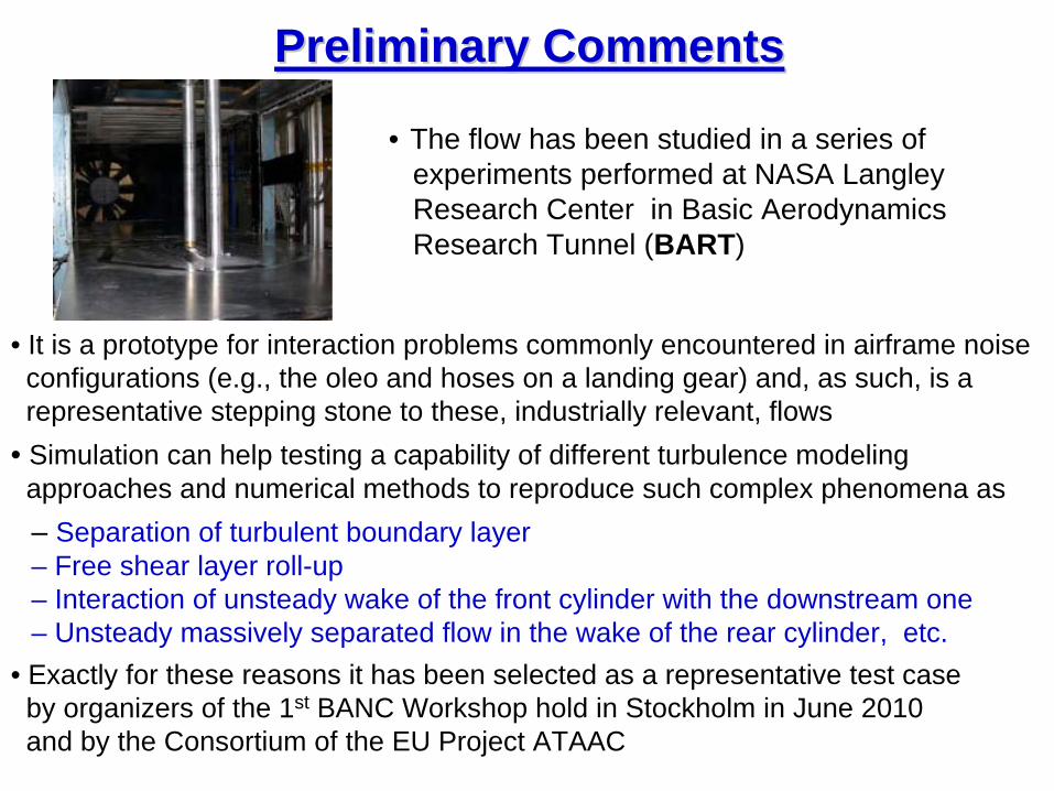
• It is a prototype for interaction problems commonly encountered in airframe noiseconfigurations (e.g., the oleo and hoses on a landing gear) and, as such, is arepresentative stepping stone to these, industrially relevant, flows

• Simulation can help testing a capability of different turbulence modelingapproaches and numerical methods to reproduce such complex phenomena as– Separation of turbulent boundary layer– Free shear layer roll-up – Interaction of unsteady wake of the front cylinder with the downstream one– Unsteady massively separated flow in the wake of the rear cylinder, etc.

• Exactly for these reasons it has been selected as a representative test caseby organizers of the 1st BANC Workshop hold in Stockholm in June 2010and by the Consortium of the EU Project ATAAC

Preliminary CommentsPreliminary Comments

• The flow has been studied in a series of experiments performed at NASA LangleyResearch Center in Basic AerodynamicsResearch Tunnel (BART)

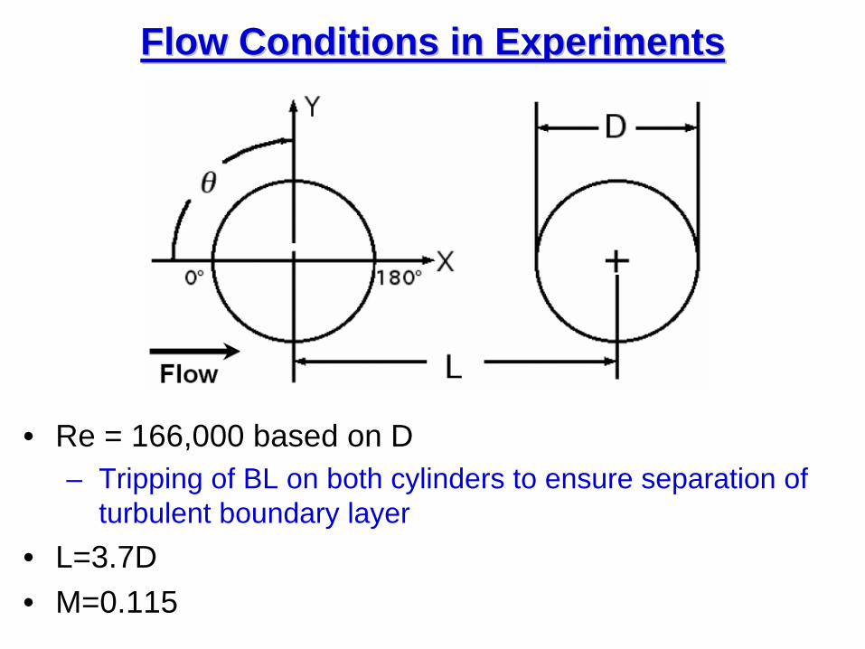
Flow Conditions in ExperimentsFlow Conditions in Experiments

• Re = 166,000 based on D– Tripping of BL on both cylinders to ensure separation of

turbulent boundary layer• L=3.7D• M=0.115

5

Simulation Approach and Numerical MethodSimulation Approach and Numerical Method• Turbulence simulation approach

– Incompressible Delayed DES (DDES) of Spalart et al. 2008• Spatial and temporal discretizations

– FV hybrid (weighted centered/upwind-biased) numerical scheme based on Rogers and Kwak flux-difference splitting method

• 4th centered / 5th upwind-biased for inviscid fluxes;• 2nd order centered for viscous fluxes; • 2nd implicit time integration (3 layer scheme)

• Boundary Conditions– Inflow: uniform streamwise and zero lateral velocity components;

eddy viscosity equal to molecular one (FT approach totransition control)

– Cylinders walls: No-slip– WT section side walls: Free-slip– Spanwise: Periodic at two span sizes of the domain: Lz=3D and 16D– Outflow: Specified pressure

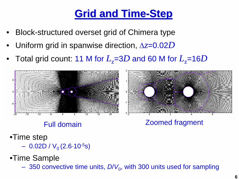
Grid and TimeGrid and Time--StepStep• Block-structured overset grid of Chimera type• Uniform grid in spanwise direction, Δz=0.02D• Total grid count: 11 M for Lz=3D and 60 M for Lz=16D

6

Full domain Zoomed fragment

•Time step– 0.02D / V0 (2.6·10-5s)

•Time Sample– 350 convective time units, D/V0 , with 300 units used for sampling

Internal Quality ChecksInternal Quality Checks

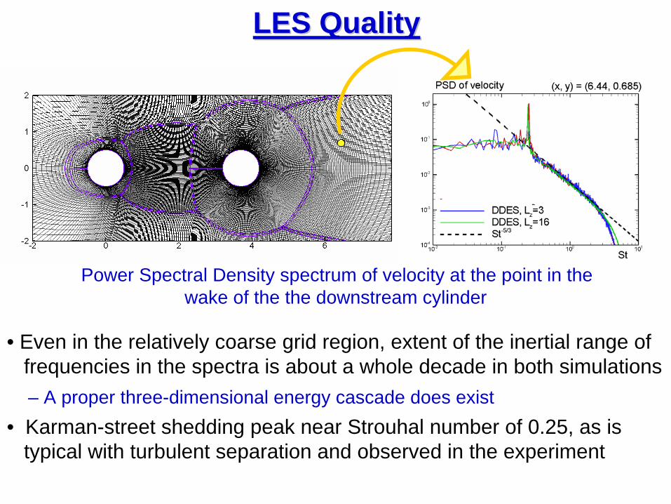
• Even in the relatively coarse grid region, extent of the inertial range offrequencies in the spectra is about a whole decade in both simulations– A proper three-dimensional energy cascade does exist

• Karman-street shedding peak near Strouhal number of 0.25, as istypical with turbulent separation and observed in the experiment

Power Spectral Density spectrum of velocity at the point in thewake of the the downstream cylinder

LES QualityLES Quality

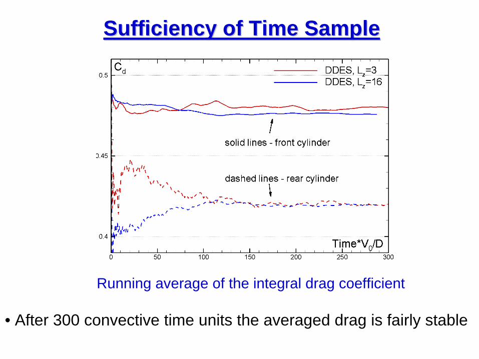
Running average of the integral drag coefficient

• After 300 convective time units the averaged drag is fairly stable

Sufficiency of Time SampleSufficiency of Time Sample

Results & Comparison with Results & Comparison with Experiment Experiment

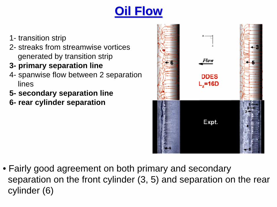
Oil FlowOil Flow

1- transition strip2- streaks from streamwise vortices

generated by transition strip3- primary separation line4- spanwise flow between 2 separation

lines 5- secondary separation line6- rear cylinder separation

• Fairly good agreement on both primary and secondaryseparation on the front cylinder (3, 5) and separation on the rearcylinder (6)

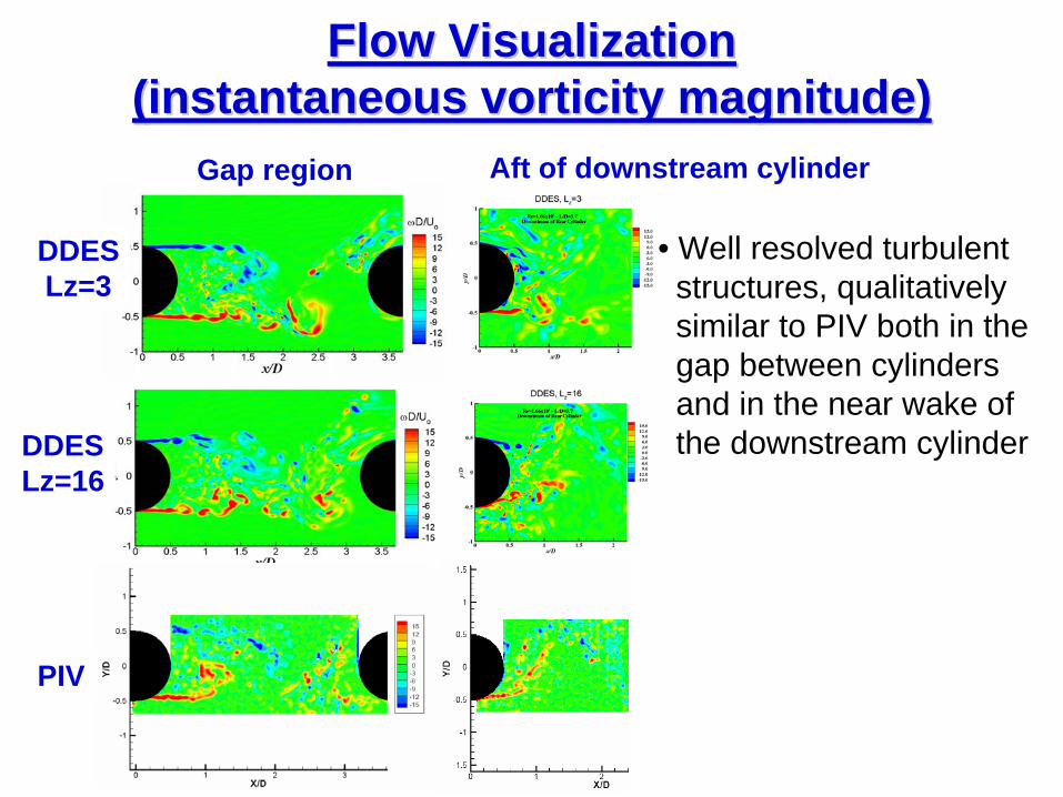
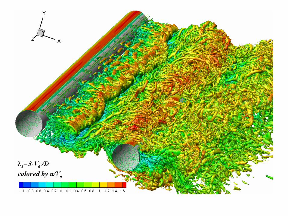
Flow VisualizationFlow Visualization (instantaneous (instantaneous vorticityvorticity magnitude)magnitude)

• Well resolved turbulentstructures, qualitativelysimilar to PIV both in thegap between cylindersand in the near wake ofthe downstream cylinderDDES

Lz=16

PIV

DDESLz=3

Gap region Aft of downstream cylinder

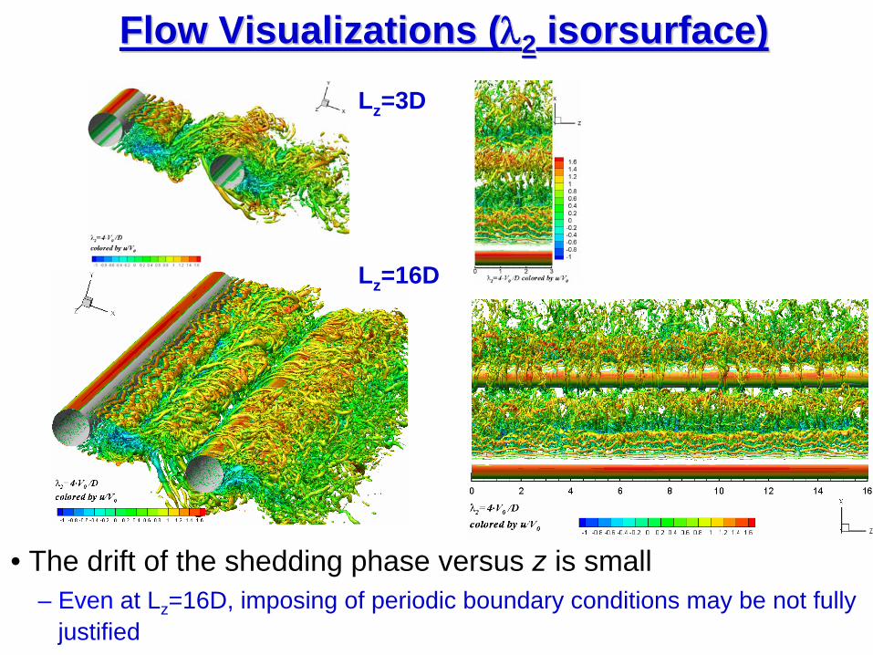
Flow Visualizations (Flow Visualizations (λλ 22 isorsurfaceisorsurface))

• The drift of the shedding phase versus z is small– Even at Lz =16D, imposing of periodic boundary conditions may be not fully

justified

Lz =3D

Lz =16D

15

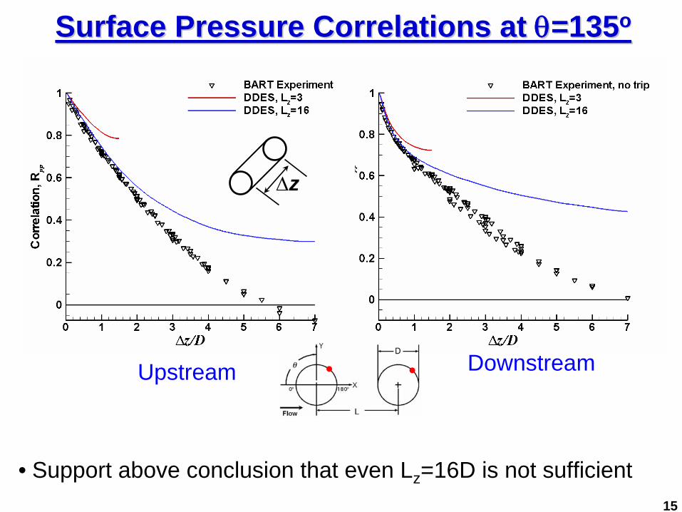
Surface Pressure Correlations at Surface Pressure Correlations at θθ=135=135oo

Upstream Downstream

Δz

• Support above conclusion that even Lz =16D is not sufficient

Upstream Downstream

16

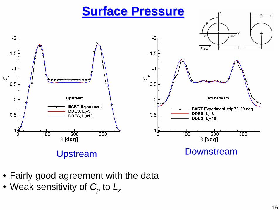
Surface PressureSurface Pressure

• Fairly good agreement with the data• Weak sensitivity of Cp to Lz

Gap Region Aft of Downstream Cylinder

17

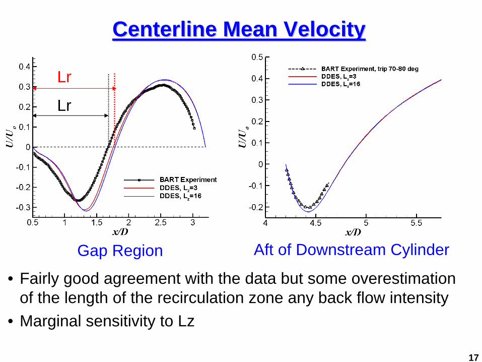
Centerline Mean VelocityCenterline Mean Velocity

• Fairly good agreement with the data but some overestimation of the length of the recirculation zone any back flow intensity

• Marginal sensitivity to Lz

Lr

Lr

18

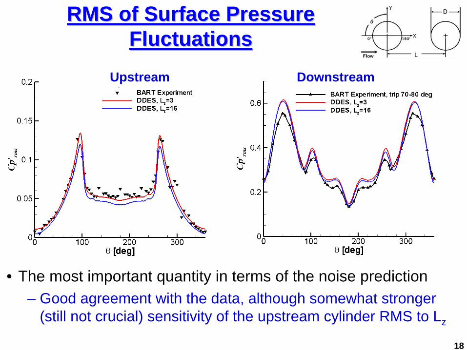
RMS of Surface Pressure RMS of Surface Pressure FluctuationsFluctuations

Upstream

• The most important quantity in terms of the noise prediction– Good agreement with the data, although somewhat stronger

(still not crucial) sensitivity of the upstream cylinder RMS to Lz

Downstream

19

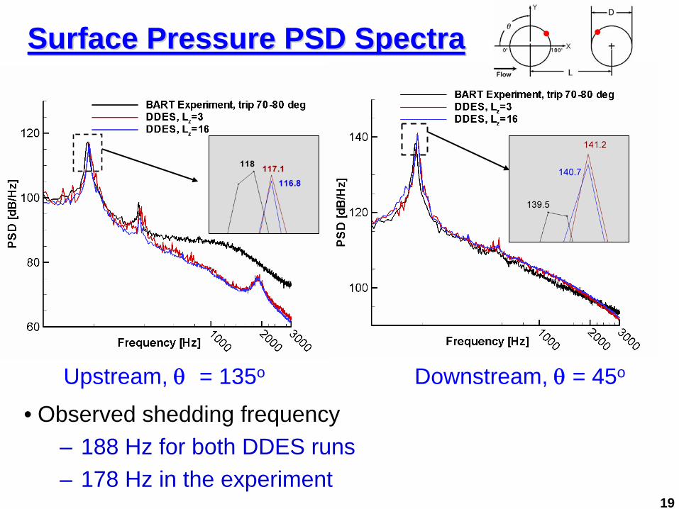
Surface Pressure PSD SpectraSurface Pressure PSD Spectra

Upstream, θ

= 135o Downstream, θ

= 45o

• Observed shedding frequency– 188 Hz for both DDES runs– 178 Hz in the experiment

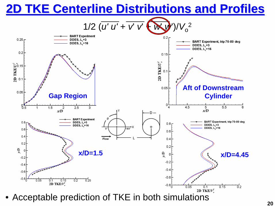
1/2 (u' u' + v' v' + w' w')/Vo2

20

2D TKE Centerline Distributions and Profiles2D TKE Centerline Distributions and Profiles

Aft of Downstream Cylinder

• Acceptable prediction of TKE in both simulations

Gap Region

x/D=1.5 x/D=4.45

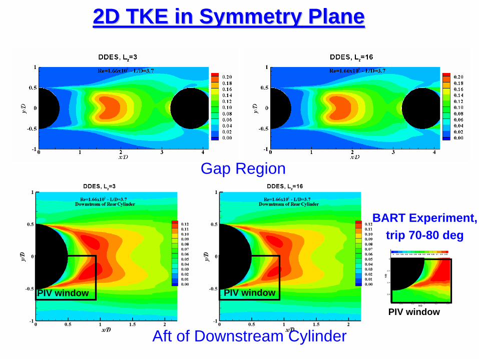
BART Experiment,trip 70-80 deg

PIV window

2D TKE in Symmetry Plane2D TKE in Symmetry Plane

Gap Region

Aft of Downstream Cylinder

PIV window

PIV window

• DDES is shown capable of providing a fairly accurateprediction of the flow

• In contrast to simulations of NASA, no significant effect ofincrease of the size of the domain in the spanwise directionfrom 3 up to 16D is observed

• Although grid and numerics used in the simulations seem tobe “good enough”, a substantial grid-refinement should beyet performed

22

Conclusions and OutlookConclusions and Outlook

• We gratefully acknowledge the computing time on the Blue Gene/P atArgonne National Laboratory (Intrepid)

• The research was funded by the Boeing Company and, partially, by the EUproject ATAAC, (ACP8-GA-2009-233710) and by the Russian Basic Research Foundation (grant No. 09-08-00126)

AcknowledgmentsAcknowledgments