Western University Western University

Scholarship@Western Scholarship@Western

Electronic Thesis and Dissertation Repository

12-8-2016 12:00 AM

Investigation of Model Predictive Control (MPC) for Steam Investigation of Model Predictive Control (MPC) for Steam

Generator Level Control in Nuclear Power Plants Generator Level Control in Nuclear Power Plants

Ahmad Taemiriosgouee, The University of Western Ontario

Supervisor: Jiang, Jin, The University of Western Ontario

A thesis submitted in partial fulfillment of the requirements for the Master of Engineering

Science degree in Electrical and Computer Engineering

© Ahmad Taemiriosgouee 2016

Follow this and additional works at: https://ir.lib.uwo.ca/etd

Part of the Controls and Control Theory Commons

Recommended Citation Recommended Citation Taemiriosgouee, Ahmad, "Investigation of Model Predictive Control (MPC) for Steam Generator Level Control in Nuclear Power Plants" (2016). Electronic Thesis and Dissertation Repository. 4378. https://ir.lib.uwo.ca/etd/4378

This Dissertation/Thesis is brought to you for free and open access by Scholarship@Western. It has been accepted for inclusion in Electronic Thesis and Dissertation Repository by an authorized administrator of Scholarship@Western. For more information, please contact wlswadmin@uwo.ca.

Abstract

The capabilities and potential of Model Predictive Control (MPC) strategies for

steam generator level (SGL) controls in nuclear power plants (NPPs) have been

investigated. The performance has been evaluated for the full operating power

range (0% to 100%). The specific operating conditions include: normal operations,

start-ups, low power operations, load-up and load rejections. These evaluations

have been carried out using a linearized steam generator dynamic model. The MPC

controllers used are based on existing methodologies. Furthermore, any potential

performance improvement through fine-tuning of some of the control parameters

based on the dynamic characteristics of the SGL has also been investigated.

In this regard, two versions of MPC strategies have been designed and simulated.

The Standard MPC (SMPC) is applied to the SGL problem first to establish the

performance baseline. An Improved MPC (IMPC), by selecting appropriate values

in the weight matrix of the objective function, has also been examined.

Both MPC strategies have been implemented in a Matlab Simulink environment.

Their performance has been evaluated against an optimized PI controller in terms

of i) set point tracking, ii) load-following in step and ramp commands, iii) figures

of merits of transient responses, iv) effectiveness in rejecting disturbance from the

steam and feed-water flow, and v) sensitivities to the noise in the feed-water flow

measurements. The performance evaluation has been done through extensive

computer simulation, and also through a set of real-time experiments on a physical

mock-up steam generator level process. The results have demonstrated potential of

the MPC based strategies; in particular, the IMPC strategy; for improving the

performance of the steam generator level control loop.

KEYWORDS: Level Control, Non-minimum-phase, Nonlinear Model Predictive

Control, Steam Generator.

ii

Acknowledgments

I am indebted to Professor Jin Jiang, who provided me with the opportunity to

pursue my study at the University of Western Ontario (UWO) and directed me in

my research and the writing of this thesis. I have learned a lot from Dr. Jiang and

am grateful to him for his support of my work. The work has been carried out at the

Department of Electrical & Computer Engineering. I would like to thank Dr. Ataul

Bari for his great support and guidance throughout the period leading up to this

thesis. I am also grateful to Drew J. Rankin for his support during the physical

simulation phase of this study. I am also grateful to Prof. Lyndon Brown for his

in-depth comments which have helped to improve the quality of the thesis.

iii

This thesis is dedicated to my lovely daughter Nastaran

iv

Table of Contents

Abstract .............................................................................................................. i

Acknowledgments............................................................................................. ii

Table of Contents ............................................................................................. iv

List of Tables .................................................................................................. vii

List of Figures ................................................................................................ viii

List of Symbols and Abbreviations.................................................................. xi

1 Introduction ................................................................................................... 1

1.1 Steam Generator Level (SGL) control ................................................... 2

1.1.1 Importance ................................................................................. 2

1.1.2 Unique dynamic characteristics ................................................. 3

1.2 Motivations for the current work ........................................................... 5

1.3 Objectives, approaches, and scope......................................................... 6

1.4 Thesis contributions ............................................................................... 7

1.5 Organization of the thesis ...................................................................... 8

2 Literature Review .......................................................................................... 9

2.1 Steam generator level control ................................................................ 9

2.2 SGL control strategies in the literature ................................................ 11

2.2.1 Auto-tuned PID controller using a MPC ................................. 12

2.2.2 Linear Quadratic Regulator (LQR) .......................................... 12

2.2.3 Fuzzy and Neuro-Fuzzy based controllers ............................... 13

2.2.4 Gain scheduled controller ........................................................ 13

2.2.5 H∞ control techniques ............................................................... 14

2.2.6 Extension of the MPC principle ............................................... 14

2.3 Summary .............................................................................................. 14

v

3 MPC for SGL Control ................................................................................. 15

3.1 Overview .............................................................................................. 15

3.2 Mathematical model of a steam generator ........................................... 16

3.3 SGL model linearization ...................................................................... 18

3.4 The MPC for SGL control ................................................................... 20

3.5 The Standard Model Predictive Control (SMPC) ................................ 23

3.6 An Improved Model Predictive Control (IMPC) ................................. 29

3.7 Summary .............................................................................................. 32

4 Simulation Studies ...................................................................................... 33

4.1 Background and objectives .................................................................. 33

4.2 Simulation set up.................................................................................. 33

4.2.1 Simulation of the SGL ............................................................. 34

4.2.2 State observer ........................................................................... 34

4.2.3 Selection of simulation scenarios............................................. 35

4.2.4 Step responses .......................................................................... 36

4.2.5 SGL subject to step changes in reactor power level ................ 44

4.2.6 SGL response subject to ramp change in reactor power .......... 46

4.2.7 SGL response subject to steam flow disturbance .................... 47

4.2.8 SGL response subject to feed-water flow disturbance ............. 51

4.2.9 SGL response subject to random measurement noise in the

FWF ......................................................................................... 53

4.3 Summary .............................................................................................. 56

5 Physical Test Results on the PLS ................................................................ 57

5.1 Background and objectives .................................................................. 57

5.2 Physical simulation set up .................................................................... 57

5.3 Selection of simulation scenarios......................................................... 59

vi

5.3.1 Step response ........................................................................... 60

5.3.2 SGL response subject to changes in reactor power level in

step ........................................................................................... 65

5.3.3 SGL response subject to changes in reactor power level in

ramp ......................................................................................... 67

5.3.4 SGL response subject to random noise in the FWF

measurements ........................................................................... 68

5.4 Summary .............................................................................................. 71

6 Conclusions and Future Work ..................................................................... 72

6.1 Contributions........................................................................................ 72

6.2 Discussions and conclusions ................................................................ 73

6.3 Future work .......................................................................................... 74

References ........................................................................................................ 75

CURRICULUM VITAE (CV) ......................................................................... 79

vii

List of Tables

Table 1 The parameters of Irving SG model over five power levels .................... 17

Table 2 SGL model linearization regions ............................................................. 19

Table 3 An example of computing IMPCQ at 5% PL .............................................. 31

Table 4 The Eigenvalues for IMPC and SMPC at PL=5% ................................... 38

Table 5 Feedback gains for IMPC and SMPC at PL=5% ..................................... 39

Table 6 Performance of IMPC, SMPC and PI strategies ...................................... 44

Table 7 Performance of IMPC, SMPC and PI strategies on the PLS ................... 65

viii

List of Figures

Fig. 1 Schematic diagram of a typical SG in a NPP [2] ........................................ 2

Fig. 2 Basic feed-back structure of MPC ............................................................. 16

Fig. 3 SGL to (a) step changes in the feed-water flow, (b) step changes in the

steam flow based on the Irving model [1] ............................................................ 18

Fig. 4 Basic feedback control structure of MPC for SGL.................................... 20

Fig. 5 Basic philosophy of a MPC ....................................................................... 21

Fig. 6 Block diagram for PI, SMPC and IMPC ................................................... 35

Fig. 7 SGL subject to a step change at PL=5% ................................................... 37

Fig. 8 Control signal subject to a step change at PL=5% .................................... 38

Fig. 9 SGL subject to a step change at PL=15% ................................................. 39

Fig. 10 Control signal subject to a step change at PL=15% ................................ 40

Fig. 11 SGL subject to a step change at PL=30% ............................................... 40

Fig. 12 Control signal subject to a step change at PL=30% ................................ 41

Fig. 13 SGL subject to a step change at PL=50% ............................................... 41

Fig. 14 Control signal subject to a step change at PL=50% ................................ 42

Fig. 15 SGL subject to a step change at PL=100% ............................................. 42

Fig. 16 Control signal subject to a step change at PL=100% .............................. 43

Fig. 17 SGL subject to multiple PL step-up changes from 5% to 22% ............... 45

Fig. 18 Control signal subject to multiple PL step-up changes from 5% to 22% 45

ix

Fig. 19 SGL subject to power level changes from 5 % to 100 %, followed by a

load rejection to 5% .............................................................................................. 46

Fig. 20 Control signal subject to power level changes from 5 % to 100 %

followed by a load rejection to 5% ....................................................................... 47

Fig. 21 SGL subject to a SF disturbance at PL=5% ............................................ 49

Fig. 22 Control signal subject to a SF disturbance at PL=5% ............................. 49

Fig. 23 SGL subject to a SF disturbance at PL=50% .......................................... 50

Fig. 24 Control signal subject to a SF disturbance at PL=50% ........................... 50

Fig. 25 SGL signal subject to FWF step-disturbances at PL=5%........................ 51

Fig. 26 Control signal subject to FWF step-disturbances at PL=5% ................... 52

Fig. 27 SGL subject to FWF step-disturbances at PL=50% ................................ 52

Fig. 28 Control signal subject to FWF step-disturbances at PL=50% ................. 53

Fig. 29 SGL subject to FWF random noise disturbance at PL=5% ..................... 54

Fig. 30 Control signal subject to FWF random noise disturbance at PL=5% ..... 55

Fig. 31 SGL subject to FWF random noise disturbance at PL=50% ................... 55

Fig. 32 Control signal subject to FWF random noise-disturbance at PL=50% ... 56

Fig. 33 The Plate Level System (PLS)................................................................. 58

Fig. 34 A schematic diagram of the PLS with a digital filter for simulating non-

minimum phase characteristics ............................................................................. 59

Fig. 35 SGL of the PLS at PL=5% ...................................................................... 61

Fig. 36 Control signal to the PLS at PL=5% ....................................................... 62

x

Fig. 37 SGL of the PLS at PL=15% .................................................................... 63

Fig. 38 Control signal to the PLS at PL=15% ..................................................... 63

Fig. 39 SGL of the PLS at PL=100% .................................................................. 64

Fig. 40 Control signal to the PLS at PL=100% ................................................... 64

Fig. 41 SGL of the PLS subject to PL step up changes from PL=5% to 22%

followed by a load rejection to PL=5% ................................................................ 66

Fig. 42 Control signal to the PLS subject to PL step up changes from PL=5% to

22% followed by a load rejection to PL=5% ........................................................ 66

Fig. 43 SGL of the PLS for PL ramp up changes from PL=5% to 80% followed

by load rejection to PL=10% ................................................................................ 67

Fig. 44 Control signal to the PLS for PL ramp up changes from PL=5% to 80%

followed by load rejection to PL=10% ................................................................. 68

Fig. 45 SGL of the PLS subject to FWF random noise at PL 5% ....................... 69

Fig. 46 Control signal to the PLS subject to FWF random noise at PL 5% ........ 69

Fig. 47 SGL of the PLS subject to FWF random noise at PL 50% ..................... 70

Fig. 48 Control signal to the PLS subject to FWF random noise at PL 50% ...... 70

xi

List of Symbols and Abbreviations

Symbols

a Scaling factor for discrete-time Laguerre functions

( ), ( ), ( ), ( ),m w v m mA B B B C Power level dependent parameters in discrete time

'( ), ' ( ), ' ( ), 'w vA B B C Power level dependent parameters in continuous time

( ), ( ),A B C Power level dependent parameters in augmented model

( )d k External disturbance (steam flow rate)

1 2 3, ,G G G Irving model parameters

( )uG s Transfer function for feed water flow

( )vG s Transfer function for steam flow

lH Laguerre functions matrix

J Performance index for optimization (for augmented model)

pJ Performance index for optimization for MPC

SMPCK Feedback control gain using SMPC

IMPCK Feedback control gain using IMPC

( )L k Laguerre functions

m Control horizon in the MPC algorithm

p Prediction horizon (number of steps in future predictions) in the MPC

N Number of terms used in the Laguerre function expansion

Power level in percentage of full power (%FP)

R A weight matrix in the cost function of predictive control

SMPCQ A weight matrix in the cost function of predictive control in SMPC

IMPCQ A weight matrix in the cost function of predictive control in IMPC

, Pair of matrices in the cost of predictive control J

wQ (s) Laplace Transform of the Feed-water flow rate

vQ (s) Laplace Transform of the Steam flow rate

wq (t) Feed-water flow rate in continuous time

xii

vq (t) Steam flow rate in continuous time

wq (k) Feed-water flow rate in discrete time

vq (k) Steam flow rate in discrete time

r Set-point function of the steam generator level

1 2, ,T Damping constant, time constant, and the period of oscillation,

respectively

U Parameter vector for the control sequence

( )u k Feed-water flow rate

,min ,max,j ju u Minimum and maximum limits for u

Parameter vector in the Laguerre expansion

( )x t System state in continuous time

( )x k System state in discrete time

,min ,max,j jx x Constraints on the states

( )x k Estimate of the system state ( )x k

,min ,max,j jy y Constraints on the steam generator level

( )y k Estimate of the steam generator level ( )y k

Y(s) Steam generator level in Laplace domain

y(t) Steam generator level in continuous time

y(k) Steam generator level in discrete time

Abbreviations

DAQ Data Acquisition

FP Full power

FWCV Feed-water Control Valve

F.W.F Feed-water Flow

HTS Heat transport system

IMPC Improved model predictive control

LPV Linear parameter varying

xiii

LQG/LTR Linear quadratic Gaussian/ Loop transfer recovery

MPC Model predictive control

MMPC Multiple model predictive control

MVPC Model varying predictive control

NPP Nuclear power plant

PL Power level

PLS Plate Level System

PLs Power levels

SG Steam generator

SGL Steam generator level

SGLC Steam generator level control

SMPC Standard model predictive control

1 Introduction

Steam Generators (SGs) in a Nuclear Power Plant (NPP) play an important role in

transferring heat from a fission process to steam in order to drive a steam turbine

for generating power. The SG in a NPP provides an important heat sink for the

reactor and for the Heat Transport System (HTS) which operates with the reactor

coolant on the primary side, and the feed-water in the secondary side. It can also be

used as heat removal systems in the event of an accident. From a safety point of

view, the SG is a major element which isolates the primary loop (containing

radioactive coolant) from the secondary loop (containing non-radioactive water and

steam) to prevent water in the two systems from intermixing. The SG also prevents

radioactive substances from leaking into the atmosphere in a NPP.

Other roles of a steam generator in a nuclear power plant can be summarized as

follows [1]:

Continuous cooling of the reactor core

Mass balancing between feed-water and steam flow rate

Preventing the carryover of impurities inside the turbine

Generating steam for the turbine to produce electricity

A schematic diagram of a typical SG is shown in Fig.1 [2]. The hot pressurized

coolant enters the inlet and passes through what is referred to as the “hot leg” of the

tube bundle. The feed-water enters the secondary side of the tube bundle at the

upper right of the SG through the feed-water inlet nozzle. The coolant passes

through an inverted U-tube heat exchanger, where thermal energy is transferred

from the primary side to the secondary side at the saturation temperature (e.g, 250o

C at 4 MPa pressure in certain NPPs) to generate steam. The primary coolant loses

thermal energy all along the U-tube. The steam passes through separators, which

ensure that the exiting steam is completely dry to protect the turbine blades from

2

damage. The water inventory in the SG can be directly measured via SG water level

gauges at the secondary side.

Fig. 1 Schematic diagram of a typical SG in a NPP [2]

1.1 Steam Generator Level (SGL) control

1.1.1 Importance

The Steam Generator Level (SGL) must be controlled within a certain range and a

desired value during both transient and steady-state operations to create a safe and

reliable environment in a NPP. Poor control of the SGL may lead to serious

consequences. If the level in the SG is too high, it may lead to the following

problems: [1], [3]

3

Increased moisture in the steam and carryover, and humidity to the turbine

side. This increases the risk of damages to the turbine blades

Increased potential for water hammer and water induction hazards in the

piping system

Reduced margin between the SGL and the SGL upper limit, which increases

the risk of a turbine trip

If the level is too low, it may lead to the following problems: [1], [3]

Decreased heat sink capability of the SG, which may lead to increased HTS

pressure and temperature

Jeopardized reactor cooling system due to the exposed tubes

Reduced heat transfer capability of removing heat from the reactor, leading

to reactor overheating

SG drying-out, raising the risk of damages in SG tubes

If the control system for the SG water level is inappropriately tuned, oscillations in

the water level may occur. Such oscillations can induce subsequent oscillations in:

instantaneous turbine output power,

feed-water and steam flow rates, and

HTS pressure and temperature.

It has been documented [1,3,4,5] that nearly 25% of emergency reactor and turbine

trips at existing NPPs are caused by poor performance in SGL control. Nearly 90%

of incidents associated with SGL occur either at low operating power levels (less

than 25% of full power), or during transient periods. This is mainly because of the

dynamic characteristics of the SGL and the relatively higher degree of steam and

feed-water flow measurement inaccuracy.

1.1.2 Unique dynamic characteristics

The dynamics of a SGL vary considerably with changes in reactor power levels. A

unique phenomenon exists particularly at low power operations, because of the

dominant reverse thermal dynamic effects known as shrink and swell. A sudden

4

increase in load will draw more steam from the SG. Naturally, one expects that the

water level will decrease. However, as more steam is drawn, the bubbles in the

water actually expand, and make the water level higher, which is counter-intuitive,

and it makes the control system more difficult to design. This phenomenon is

known as ̀ swell`. A sudden decrease in load produces exactly the opposite response

in the water level, which is called `shrink`. In the control system community, this

behavior can be characterized by non-minimal phase dynamics in the transfer

functions.

To leave sufficient operating range, it is not desirable to operate the SG at a high

water level during low power operations since the SG could be subjected to an

unexpectedly large step increase in the steam demand causing a large swell effect.

By maintaining the SGL relatively low under a low power condition, one may

accommodate a relatively large swell effect in the level without causing any risk of

possible turbine trip due to inventory carryover to the turbine. Similarly, it is not

desirable to operate the SG at a low water level during high power operations since

the SG may be subjected to an unexpectedly large step decrease in the steam

demand, causing a large shrink to uncover the HTS U-tubes in the heat exchanger.

Consequently, by maintaining the SG water level relatively high at high power, one

can accommodate a relatively large shrink in level without increasing the risk of

exposing the U-tube heat exchanger. Hence, the above guidelines should be

followed in selecting swell based set points, i.e., the desirable set point values for

the steam generator levels.

The swell and shrink effects decrease as the operating power level increases. This

is one of the main reasons that the conventional Steam Generator Level Control

(SGLC) schemes (single-element/three-element control) cannot possibly cover the

entire operating power range (from 0% to 100%). Other characteristics of the SGL

that may affect controller design include [1]:

• highly nonlinear behavior, especially during low power operations,

5

• tight constraints on the SG input (feed-water flow rate) and the SG output

(SGL), and

• inaccurate and noisy measurements for feed-water flow rate and steam flow

rate during low power operations.

It may be noted that due to the lack of an effective control system that can cover

the entire operating power range, manual control is often applied to the SGL system

during the start-up and the low power operations in many existing NPPs.

1.2 Motivations for the current work

The SGL control system designs have been extensively investigated and substantial

efforts have been made to prevent costly reactor shutdowns caused by the SGL

control system. Over the last thirty years, a great deal of research has been done

with the SGLC, and many advanced model-based SGL controller design have been

proposed in the literature that include

Model predictive control (MPC)

Model reference adaptive PID

Linear quadratic regulator method

Fuzzy and neuro-fuzzy control

Artificial neural network based controller

H∞ control techniques

Gain-scheduling controller

Extension of MPC principle

Auto-tuned PID

Auto adaptive predictive controller

Model based control strategies for the SGL control presented in the existing

literature often investigate the performance of the given scheme on a limited

number of SGL control scenarios. Much of the literature does not evaluate the

performance of the control scheme during the start-up and the low power

6

operations. Extensive evaluation for the SGLC performance under tight constraints,

and under steam and feed-water flow disturbances are often not done. Furthermore,

the capability of the SGL control for load following in steps and in ramps, as well

as for load rejections are also not properly investigated and evaluated in most of the

existing literature. It is noted that, despite many advanced control techniques

developed for SGL, they have rarely been used in NPPs, as their ability to handle

the entire range of operating modes (including start-up, low power operations, and

emergency shut-downs) has not yet been extensively evaluated and demonstrated.

For a proper evaluation, a control scheme must be investigated with respect to all

operating and transient conditions of a SG. Therefore, it is reasonable to perform

an in-depth study in order to understand the capability of a given control scheme to

deal with the challenges in the SGL control in NPPs. One model based advanced

control strategy that has been used in many other industrial control applications is

the Model Predictive Control (MPC). The MPC based approaches make use of the

“best knowledge” of the process dynamic in order to deliver an effective

performance by the control system. Due to the capabilities of the MPC based

approaches to handle challenging control problems, the MPC has been selected for

an in-depth evaluation, while applying it in the SGL control systems in NPPs.

Furthermore, in addition to the detailed performance evaluation of existing

advanced MPC controllers, it would be interesting to investigate if a MPC

controller performance can be improved by applying customized fine-tuning of the

control parameters by taking into account the specific characteristics of the SGL in

NPPs at different power levels.

1.3 Objectives, approaches, and scope

The objective of this study is to perform a detailed evaluation of the MPC based

strategies for the SGL control in NPPs. Performance has been evaluated for a MPC

controller based on existing advanced methodologies. Furthermore, any

performance improvements that can be achieved by the fine-tuning of the control

parameters (based on the characteristics of the SGL) of the existing MPC

7

approaches has also been investigated. The investigation have been performed to

cover all operating conditions of a SG in a NPP that include normal operations, as

well as start-ups, low power operations, load-up and load rejections.

The control performance of the MPC based methodologies have been evaluated

through computer simulation and through a set of tests on a physical mock-up steam

generator level process that uses a metal plate and pressurized air to simulate the

effect of a SGL in a NPP. This mock-up steam generator has been referred to as the

Plate Level System (PLS) in this thesis. The PLS closely simulates the

characteristics of an actual SGL (based on Irving model) at different power levels.

The scope of this work has been limited to an in-depth performance evaluation of

existing advanced MPC based methodologies for SGLC in NPPs. It is well known

that the MPC based approaches rely heavily on the model of the underlying process.

Although there are a few models for the SGL exists in the literature; however, this

study has limited its scope to the Irving model for the SGL. Therefore, the results

reported in this study are all based on the Irving model. Furthermore, the Irving

model specifies the SGL model parameters only at five different power levels (5%,

15%, 30%, 50%, and 100%). The MPC based strategies implemented for evaluation

in this study are centered around these power levels only.

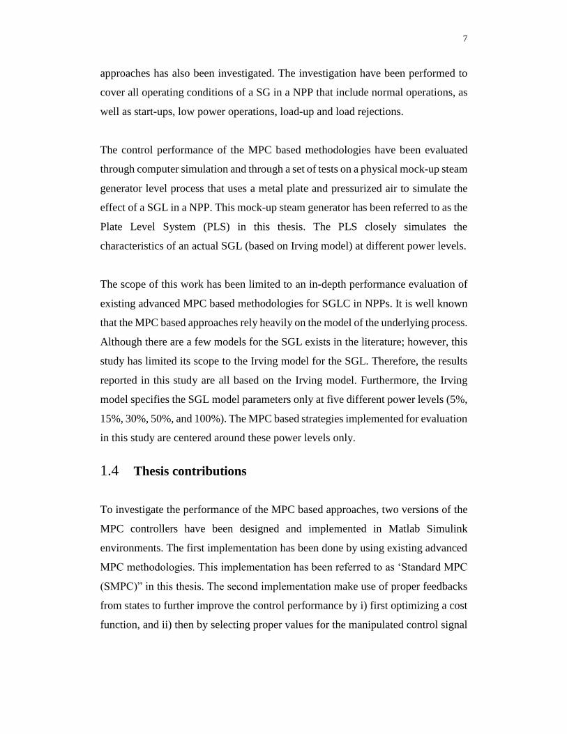
1.4 Thesis contributions

To investigate the performance of the MPC based approaches, two versions of the

MPC controllers have been designed and implemented in Matlab Simulink

environments. The first implementation has been done by using existing advanced

MPC methodologies. This implementation has been referred to as ‘Standard MPC

(SMPC)” in this thesis. The second implementation make use of proper feedbacks

from states to further improve the control performance by i) first optimizing a cost

function, and ii) then by selecting proper values for the manipulated control signal

8

( )u k . This control signal is then applied to the Feed-water Control Valve (FWCV).

The second MPC has been referred to as “Improved MPC (IMPC)”.

Both computer simulation, and the Plate Level System (PLS) physical tests have

been performed to include all operating conditions of a real NPP. The performance

has been evaluated in terms of several performance measures that include set point

tracking, overshoot, undershoot, settling time subject to set point change, transient

response and load following.

During the process of implementation, the following contributions are made:

Linearization of the SGL model and design of power level dependent

parameters for SMPC/IMPC schemes

Selection of an appropriate cost function J that can be used to minimize

the prediction of the error signal over the future horizon of 𝑝, and also

minimizes the usage of the controller outputs in the least-square sense

Application of “Laguerre functions” as an efficient tool for approximating

stable dynamic systems for the SMPC and the IMPC controller structures.

Presented a simple approach to define the weight matrix IMPCQ for IMPC.

1.5 Organization of the thesis

The organization of the thesis is as follows: Chapter 1 introduces the importance of

the SGL control in nuclear power plants, and has outlined the work done in this

thesis. In Chapter 2, an overview of the steam generator level control, and a brief

literature review are presented. In Chapter 3, the details of SMPC and IMPC

methodologies, along with the mathematical model of the SGL are discussed.

Model linearization is also presented in Chapter 3. Performance of the SMPC and

the IMPC methodologies have been investigated through computer simulation in

Chapter 4. The results of the experiment on the PLS are presented in Chapter 5.

And finally, conclusions are drawn in Chapter 6 with a brief discussion.

9

2 Literature Review

2.1 Steam generator level control

To maintain a constant water mass inventory in the SG at different power levels,

and to reduce the SGL fluctuations (due to, e.g., swell or shrink in transient modes

load following, reactor set-back, and step-back), the SGL set-point needs to be

calculated in a dynamic manner and adjusted according to the operational power

level. A dynamic SGL set-point allows the SGL control system to react in the same

direction as the power change. In a fixed SGL set-point, the SGL would rise when

the power is increased suddenly (due to the swell effect). In a fixed set-point

system, this level rise would be opposed by the feed-water supply decrease in an

attempt to lower the SGL back to the fixed set-point. Now, when the temporary

swell effect subsides, the collapse of the steam bubbles and the decrease in the

inventory supply would have to be reversed in order to supply more feed-water at

the increased load in an attempt to maintain the desired inventory. If the set-point

of the SGL is made dynamic, the above scenario can be effectively reduced. The

original steam demand increase will cause a swell effect but, at the same time, the

increase in power level would be recognized to request a high SGL set-point. As a

result, the swell effect (level increase) can be matched by the level set-point

increase so that little-to-no change in the control signal would be initiated at the

onset of such disturbances. More specifically, the difficulties in designing an

effective level control system for a SG can be summarized as follows:

Nonlinear plant characteristics

The dynamic behaviors of a SG are highly nonlinear. A set of linearized dynamic

models can be obtained at different reactor power levels. However, the parameters

in these linearized models vary significantly as the reactor power changes. The

nonlinear process dynamics complicate the design of an effective SGL control

system. A possible solution is to design a set of controllers for different power

levels and then to apply “gain-scheduling” techniques in order to select an

appropriate controller based on the operating power level.

10

Non-minimum-phase plant characteristics

A SG exhibits inverse response behavior, which is represented by a non-minimum

phase dynamic process. This is particularly predominant at the low operating power

range. This non-minimum phase characteristic limits the achievable system

performance, and can significantly complicate the design process of an effective

SGL control system.

Flow measurement errors

It is well known that at low power operations (0-25% of the full power, FP), the

measurements of the main steam-flow and the feed-water flow are noisy and

unreliable. The SGL is more sensitive to disturbances at low power levels. As a

result, the SGL control at low power levels is even more challenging.

Tight performance constraints

The water level in a SG has to be maintained within specific limits in order to avoid

turbine and reactor trips. Moreover, transients or oscillations in the level must be

minimized to prevent turbine and reactor power oscillation. This problem is

compounded by a lack of accurate information on the feed-water flow rate and the

steam flow rate for the control system to use. In practice, there are explicit limits

due to physical constraints on the magnitude of change in the feed-water flow rate.

It is noted that conventional three-element controllers may not be able to handle the

SGL effectively at low power level operations. This is because, in addition to the

nonlinearity and non-minimum phases, at low power, both steam and feed-water

flow rate signals become noisy and un-reliable. This prevents the three-element

controller from stabilizing the system. The controller, with only proportional and

integral water level measurement terms, lacks the predictive capability to anticipate

the reverse dynamics of the water level, and therefore results in instabilities.

11

2.2 SGL control strategies in the literature

The SGL control designs literature has spread over the last thirty years. Many

advanced design approaches have been proposed in the literature in order to solve

the SGL control problems. For example, the design of a suboptimal controller using

linear output feedback control [5]. A PID control strategy is proposed in [7] which

uses an observer to estimate the water inventory. A more general gain-scheduled

linear quadratic Gaussian with loop transfer recovery (LQG/LTR) controller is

proposed in [3]. A SGL control system based on fuzzy logic principles has also

been investigated. In fact, a fuzzy logic based SGL controller has been installed at

the Fugen NPP [8]. A neuro-fuzzy controller is proposed in [9], which uses a

multilayer artificial neural network with special types of fuzzifier, inference engine,

and defuzzifier. A robust fuzzy logic gain-scheduler is designed in [10] based on

the synthesis of fuzzy inference and H∞ control techniques. A fuzzy logic controller

which is tuned off-line with genetic algorithms using SGL, feed-water and steam

flow rate signals is proposed in [11].

A gain-scheduling controller has been proposed in [12]. A novel architecture for

integrating artificial neural networks with industrial controllers is proposed for use

in predictive control of a SG [13]. In this method, a PID controller is used to control

the process and a recurrent neural network is used to model the process as a multi-

step-ahead predictor. An adaptive predictive controller is proposed in [14], where

a recursive least-squares parameter estimation algorithm is used to estimate the

unknown parameters of the SG model. The obtained model is then used to design a

generalized predictive controller.

MPC based controls for the SGL has also been presented in the literature. Irving et

al. developed a linearized model with power-dependent parameters in order to

describe the U-tube SG dynamics over the entire operating power range. Many

model based controllers proposed in the literature has used the Irving model as the

SGL model in order to evaluate the performance of the proposed controller. A

12

controller based on an extension of the MPC principle is developed in [15]. An

auto-tuned PID controller using a MPC method is also investigated in [16].

In the following, details of the literature survey that establishes concepts and

techniques related to advanced control system design for SGL are discussed.

2.2.1 Auto-tuned PID controller using a MPC

In an auto-tuned PID controller, PID control gains are automatically tuned to

overcome the drawbacks of the conventional PID controller with fixed control

gains. This is done by changing the input-weighting factor according to the power

level using a MPC method. This approach has been investigated for the SGL by

Man Gyun Na [17]. An MPC-based PID controller has been derived from the

second order linear model of a process. The SG has been described by the well-

known 4th order linear model which consists of the mass capacity, reverse dynamics

and mechanical oscillations terms. But the important terms in this linear model are

the mass capacity and reverse dynamics terms, both of which can be described by

a 2nd order linear system. The proposed controller was applied to a linear model of

the SG. The parameters of a linear model for the SG can be changed according to

the operation power level.

2.2.2 Linear Quadratic Regulator (LQR)

The Linear Quadratic Regulator (LQR) controller is developed using local

linearization of the SG model and then scheduling gain to cover the entire range

[16]. Le Wei and Fang Fang have proposed a H∞-based LQR control for the SGL

[18]. A continuous time model of the SGL is used, and LQR and H∞-based control

scheme technique is applied to design an optimum controller that forces the SGL

to follow a desired set point. The Irving Model is used for the SGL. It has been

shown in [6] that the proposed approach can provide set point tracking ability of

the SGL at different loads.

13

2.2.3 Fuzzy and Neuro-Fuzzy based controllers

An adaptive neuro-fuzzy logic controller (NFLC) can also be used for SGL control.

B.H. Cho and H.C. No have proposed a design of stability–investigated neuro-fuzzy

logic controllers for nuclear steam generators [9]. A neuro-fuzzy algorithm, which

is implemented by using a multilayer neural network with special types of fuzzifier,

inference engine and defuzzifier, is applied to the SGL. This type of controllers has

the structural advantage that arbitrary two-input, single-output linear controllers

can be adequately mapped into a set of specific control rules. In order to design a

stability-investigated NFLC, the stable sector of the given linear gain is obtained

from Lyapunov's stability criteria. Then this sector is mapped into two linear rule

tables that are used as the limits of NFLC control rules. The automatic generation

of NFLC rule tables is accomplished by using the back-error-propagation (BEP)

algorithm. There are two separate paths for the error back propagation in the SGL.

One path considers the level dynamics depending on the SG capacity, and the other

takes into account the reverse dynamics of the SG. The amounts of error back

propagated through these paths show opposite effects in the BEP algorithm from

each other for the swell-shrink phenomenon.

2.2.4 Gain scheduled controller

In a gain scheduled controller, the controller parameters may vary according to

system operations. The control law is in the form of a parameter-dependent

nonlinear state-feedback control. Kim et al. have proposed a gain–scheduled L2

control strategy for nuclear steam generator SGL [12], and have designed a

nonlinear gain-scheduled controller for the SGL which covers the entire operating

envelope. Numerically linearized models of the SGL have been developed using a

validated nonlinear model that covers its entire operating envelope. The linear

quadratic Gaussian with loop transfer recovery (LQG/LTR) method is used to

design dynamic compensators for each of the linearized models. The various

compensator matrices are fitted to a scheduling variable, namely, the temperature

difference between the primary side hot- and cold-leg temperatures, resulting in a

gain-scheduled nonlinear compensator. The performance of the gain-scheduled

14

compensator (GSC) is systematically investigated via transient response simulation

using the nonlinear SGL model.

2.2.5 H∞ control techniques

J. J. Sohn and P. H. Seong have presented a robust H∞ controller for the feed-water

system of the Korean Standard Nuclear Power Plant (KSNP) [19]. A series of

experiments has been performed using the developed thermal–hydraulic model in

order to acquire the input–output data sets, which represent steam generator

characteristics. These data sets are utilized to build simplified steam generator

models for control via a system identification algorithm. The representative robust

controllers for the selected models are designed utilizing the loop-

shaping H∞ design technique and, the robustness and performance of the proposed

controllers are validated and compared against those of PI (proportional–integral)

controller.

2.2.6 Extension of the MPC principle

MPC is a control strategy in which the current control action is obtained at each

sampling time and a finite horizon open-loop optimal control problem, by using the

current state of the plant as the initial state. The optimization algorithm uses the

predicted process outputs in order to find the sequence of process inputs values

(over a future interval known as the “control move horizon”) that solves a

predefined constrained optimization problem. Then the optimization yields an

optimal control sequence. Kothare et al. have proposed “Level control in the steam

generator of a nuclear power plant,” [6], and have presented a framework for

addressing this problem based on an extension of the standard linear model

predictive control algorithm to linear parameter varying systems.

2.3 Summary

The characteristics of the SGL, and the factors that may affect the performance of

a SGL control system have been reviewed in this chapter. A number of advanced

methodologies for the SGL control proposed in the literature has also been

reviewed.

15

3 MPC for SGL Control

3.1 Overview

The Model predictive control (MPC) has been widely investigated and used in the

process industry as an advanced control methodology. The MPC methodology has

received significant attention for optimizing the performance of control systems,

such as the SGL control due to several advantages that include

the ability of the MPC design to yield high performance control systems capable

of operating without operator interventions, and

the ability to allow constraints to be imposed on inputs, states and outputs.

The MPC uses predictions of future behavior of the process to make anticipated

control decisions. This prediction capability allows for optimally solving a control

problem on line, where the difference between the predicted output and the desired

reference is minimized over a future horizon. The control problem can be subjected

to constraints, on the manipulated inputs and outputs. The MPC utilizes a process

model to make a prediction of future plant behavior, and to compute the appropriate

corrective control action required to drive the predicted output as close as possible

to the desired target value (set-point). The objective is to find the future trend for

the input (control actions) that moves the future trend of the output so that it

approaches the desired reference trajectory.

In a MPC scheme, the current control action is obtained by solving a finite horizon

open-loop optimal control problem at each sampling instant, by using the current

state of the plant as the initial state. The optimization algorithm uses the predicted

process outputs in order to find the sequence of process input values (over a future

interval known as control move horizon) that solves a predefined constrained

optimization problem. Then the optimization yields an optimal control sequence and

the first control in this sequence is applied to the plant. Such a principle,

characterizing the basic philosophy of MPC for SGL is illustrated in Fig. 2 [20].

16

Controller output

to processProcess

Optimizer &

Controller

Process output

predictionPredictor

Set point

Process output

Fig. 2 Basic feed-back structure of MPC

The MPC based methodologies require a model of the process. More accurate

models lead to more enhanced control performance of the MPC. In the following,

the SG model used in this work is discussed.

3.2 Mathematical model of a steam generator

The design of an effective controller depends on the availability of accurate

mathematical models describing the plant dynamics. The model should be accurate

enough, and be sufficiently simple but still be able to capture the essential SG

dynamics. In this research, the Irving model [1], [3] is used because it has met the

above criteria and has widely been used in the design and evaluation of SG control

systems. The Irving model captures the non-minimum phase behavior of the SG

level.

The Irving model is a linear fourth-order dynamic model whose parameters depend

on the reactor/turbine power level. The transfer function relating the feed-water

flow rate, ( )wq s and the steam flow rate, ( )vq s to the SG water level, ( )Y s can be

expressed as [1]:

17

1 2

2

3

2 2 2 1 2

1 1

( ) ( ( ) ( )) ( ( ) ( ))(1 )

( )4 2

w v w v

w

G GY s Q s Q s Q s Q s

s s

G sQ s

T s s

(1)

where ( )Y s represents the SG level, 1 , 2 and T are the damping time constants

and the period of the mechanical oscillation, respectively. The first term in Eqn. (1)

represents the effect of any mass imbalance (feed-water vs steam flow) in the SG

level. It takes into account the level change due to the mass difference from the

feed-water inlet to the steam outlet. 1G is a positive constant independent of the

power level. 2G is the magnitude of the swell or shrink due to the feed-water or

steam flow rates, and is a positive parameter which is also dependent on the power

level. 3G is the magnitude of the mechanical oscillation, and is a function of the

power level. The parameter 3G is positive and is also a function of the power level.

Irving model specified the parameters at five different power levels, 5%, 15%, 30%,

50% and 100%. These parameters are listed in Table 1. [1].

Table 1 The parameters of Irving SG model over five power levels

5% 15% 30% 50% 100%

1G 0.058 0.058 0.058 0.058 0.058

2G 9.63 4.46 1.83 1.05 0.47

3G 0.181 0.226 0.310 0.215 0.105

1 (sec) 41.9 26.3 43.4 34.8 28.6

2 (sec) 48.4 21.5 4.5 3.6 3.4

T (sec) 119.6 60.5 17.7 14.2 11.7

( / sec)vq kg 57.4 180.8 381.8 660.0 1434.7

18

Fig. 3 SGL to (a) step changes in the feed-water flow, (b) step changes in the

steam flow based on the Irving model [1]

The responses of the SGL to step changes in the feed-water flow rate and the steam

flow rate at different power levels, based on the Irving model, are shown in Fig. 3

[1]. The inverse response behavior, and the nonlinear characteristics of the SGL are

clearly observed in the figure, especially at the low power levels. For example, at

5% FP, when the feed-water flow rate is increased, the level response first

undergoes undershoot, before rising up (Fig. 3(a)). Similar responses, but in the

reverse direction, are seen in Fig. 3(b) when the steam flow rate is increased.

3.3 SGL model linearization

To design a control algorithm for the SGL, the SG model needs to be linearized.

The dynamics of the SGL under different power levels are different, and hence,

different sets of parameters have to be used.

In this investigation, five different power levels, based on the Irving model, are

considered. The corresponding parameters under these power levels are determined

through system estimation and model-matching techniques. The Irving model

linearized in this study may be viewed as five piecewise Linear Parameter Varying

(LPV) models, to cover five power regions shown in Table 2.

19

Table 2 SGL model linearization regions

Region # Power level covered

Region 1 0% 8%

Region 2 8% 20%

Region 3 20% 40%

Region 4 40% 75%

Region 5 75% 100%

From Eqn. (1), one can represent the system as:

31 2

2 2 2 2 2

2 1 1

1 2

2

( ) ,(1 ) 4 2

( )(1 )

u

v

G sG GG s

s s T s s

G GG s

s s

(2)

where ( )uG s and ( )vG s are the transfer functions. By using the linearization

method to identify the SGL model within a power region, the model is assumed to

be linear and time-invariant. The state equations of the Irving's SG model are as

follows:

1 1

1 22 2 2

2

1

3 1 3 4 3

2 2

4 1 3

1 2 3

( ) ( ( ) ( ))

( ) ( ) ( ( ) ( ))

( ) 2 ( ) ( ) ( )

( ) 4 ( )

( ) ( ) ( ) ( )

w v

w v

w

x t G q t q t

Gx t x t q t q t

x t x t x t G q t

x t T x t

y t x t x t x t

(3)

20

Denoting the feed-water and the steam flow rates by ( ) ( )wu t q t and ( ) ( )vd t q t

Eqn. (1) can be converted into the following state space form in continuous

domain:

( ) '( ) ( ) '( ) ( ) ' ( ) ( )

( ) ' ( )

dx t A x t B u t B d t

y t C x t

(4)

1 1

22 2 2

33 34 3

0 0 0 0

0 0 0'( ) , '( ) , ' ( ) , ' 1 1 1 0

0 0 0

0 0 1 0 0 0

d

b b

a b bA B B C

a a b

(5)

where

2 2 2

34 1

1 1 2 2 2 3 3

22 2

1

33 1

( ) 4 ( )

( ), / ( ), ( )

1 / ( )

2 / ( )

a T

b G b G b G

a

a

(6)

3.4 The MPC for SGL control

The MPC controller for the SGL computes the manipulated control signal at each

sampling time by solving a finite horizon open-loop optimal control problem, using

the states of the plant. A sequence of optimal control signals is computed. The basic

feedback control structure of MPC for SGL in shown in Fig. 4.

Fig. 4 Basic feedback control structure of MPC for SGL

y

S.F

Set Point

Irving Model Gv

MPC FWCV Gu

+

+

' ''( ), ( ), ( )w vA B B

U

21

The MPC uses the SGL model to predict the future response of the SGL. The basic

philosophy of MPC is shown in Fig. 5. The SGL model is used to predict the future

states and output ( ), ( ), 1,...x k i k y k i k i p of the system over the time-

horizon p , as shown in Fig. 5. When the manipulated variable (feed water flow

rate) ( ), 0,1,... 1u k i k i m is changed over some future time-horizon, i.e., the

control horizon m , using these predictions, m control signals

( ), 0,1,... 1u k i k i m are computed to minimize the performance index over the

prediction horizon .p The first control signal (action) in the sequence, i.e., ( | )u k k

, is then applied to the Feed-water Control Valve (FWCV). The remaining optimal

inputs are discarded, and a new optimal control problem is solved at each sampling

time.

Fig. 5 Basic philosophy of a MPC

The cost function can be defined as the quadratic error between the future reference

variable and the future controlled variable within the chosen discrete time horizon

m as follows:

22

1

1 1

1 1

( ) ( ( ) ( )) ( ( ) ( ))

( ) ( ) ( ) ( )

pT

p y

i

m mT T

u u

i i

J k r k i k y k i k Q r k i k y k i k

u k i k R u k i k u k i k R u k i k

(7)

where ( )r k is the SGL set-point, ( )y k is the SGL measurement (controlled

variable), u is feed-water flow rate (manipulated variable) and , , 0y u uQ R R are

the weighting matrix. The performance-index or cost-function ( )pJ k in Eqn. (7)

reflects the tracking error between the reference and the measured SGL. It also

includes the control effort in terms of signals going to the FWCV. Subject to the

following constraints on the control input, ( ), 0,1,... 1u k i k i m , states and

output ( ), ( ), 1,...x k i k y k i k i p :

,min ,max( ) 1,2, , , 0,1,....., 1j j j uu u k i k u j n i m

(8)

,max( ) 1,2, , , 0,1,....., 1j j uu k i k u j n i m

(9)

where ,minju and ,maxju are minimum and maximum limits of control signal, and

( ) ( ) ( 1 )u k i k u k i k u k i k

Constraints on the output of the SGL and the states:

,min ,max( ) 1,2, , , 0,1,.....,j j j yy y k i k y j n i p

(10)

,min ,max( ) 1,2, , , 0,1,.....,j j j xx x k i k x j n i p (11)

23

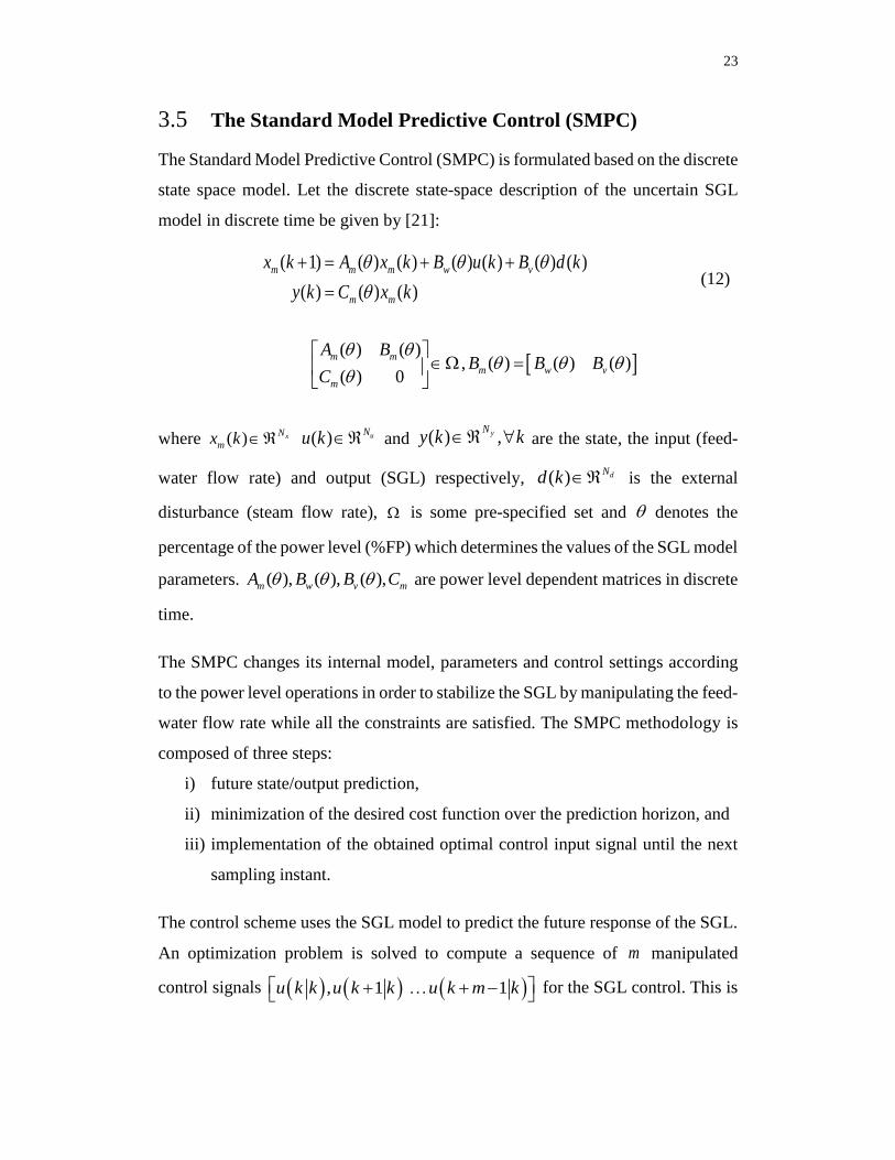
3.5 The Standard Model Predictive Control (SMPC)

The Standard Model Predictive Control (SMPC) is formulated based on the discrete

state space model. Let the discrete state-space description of the uncertain SGL

model in discrete time be given by [21]:

( 1) ( ) ( ) ( ) ( ) ( ) ( )

( ) ( ) ( )

m m m w v

m m

x k A x k B u k B d k

y k C x k

(12)

( ) ( )

, ( ) ( ) ( )( ) 0

m m

m w v

m

A BB B B

C

where ( ) xN

mx k ( ) uNu k and ( ) ,yN

y k k are the state, the input (feed-

water flow rate) and output (SGL) respectively, ( ) dNd k is the external

disturbance (steam flow rate), is some pre-specified set and denotes the

percentage of the power level (%FP) which determines the values of the SGL model

parameters. ( ), ( ), ( ),m w v mA B B C are power level dependent matrices in discrete

time.

The SMPC changes its internal model, parameters and control settings according

to the power level operations in order to stabilize the SGL by manipulating the feed-

water flow rate while all the constraints are satisfied. The SMPC methodology is

composed of three steps:

i) future state/output prediction,

ii) minimization of the desired cost function over the prediction horizon, and

iii) implementation of the obtained optimal control input signal until the next

sampling instant.

The control scheme uses the SGL model to predict the future response of the SGL.

An optimization problem is solved to compute a sequence of m manipulated

control signals , 1 1u k k u k k u k m k for the SGL control. This is

24

done by minimizing an appropriate cost function such that the p predicted outputs

1 , 2 y k k y k k y k p k follow the predefined trajectory.

The state-space description of the SGL model in discrete time is given by:

( 1) ( ) ( ) ( ) ( ) ( ) ( )

( ) ( ) ( )

( 1) ( 1) ( ), ( ) ( ) ( 1)

m m m w v

m m

m m m m m m

x k A x k B u k B d k

y k C x k

x k x k x k x k x k x k

(13)

The state-space discrete model in Eq. (13) is formulated into an augmented model

by choosing a new state variable vector, [ ( ) ( )]T

mx k y k . The augmented model

is given as follows [21]:

( 1) ( )

0( 1) ( )( ) ( ) ,

1( 1) ( )

( )( ) 0 0 0 0 1 ,

( )

x k x kA B

Tm w vm m

m m w v

C

m

A B Bx k x ku k d k

C A CB CBy k y k

x ky k

y k

(14)

In the above definition of the SMPC methodology, the following can be noted:

1. The mass flow is balanced using feedback from state

1 1( ) ( ( ) ( ))w vx k G q k q k

2. Swell/ shrink effects are minimized during different operation modes by

using feedback from state2

2

2

( ) ( ( ) ( ))w v

Gx k q k q k

3. Transient response is improved by using feedback from states

2 2 2

3 3 4 1 3( ) ( ), ( ) 4 ( )wx k G q k x k T x k

4. The SGL Model parameters vary as a function of the power level, and

the SMPC uses power level dependent SGL model

25

5. Steady-state errors are minimized over the future horizon of 𝑝, and the

size of the control move is minimized over the control horizon, m, by

minimizing the cost function for augmented model J in Eqn. (21).

The SMPC uses a set of discrete Laguerre functions. The Laguerre function is used

for its known ability to speed up the convergence of the control signal, ( )u k ,

which enables the set point error e(k) to converge to zero. The core technique is to

use additional tunable parameters (scaling factor for discrete-time Laguerre

functions) and N (number of terms used in Laguerre function expansion), while

optimizing the difference of ( )u k .

Laguerre functions are expressed in a vector form as:

1 2( ) [ ( ) ( ) . . . ( )]T

NL k l k l k l k

The set of discrete-time Laguerre functions satisfies the following difference

equation:

( 1) ( ),lL k H L k (15)

where matrix lH is N N and is a function of parameters a and 2(1 )a .

Initial condition is given by:

2 3 1 1(0) [1 . . . ( 1) ]T N NL a a a a (16)

2 3

2

0 0 0

0 0, (0) 1

- 0

-

TT

lH L

(17)

Laguerre functions used in the SMPC methodology to compute a series of control

signals:

26

1

( ) ( ) ( ) ( )

( ) ( )

NT

i j i j i

j

T

i

u k k c k l k L k

u k k L k

(18)

where consists of N Laguerre coefficients:

1 1[ . . . ] ,T

Nc c c

With initial state variable ( )x k , the prediction of the future state variable, ( )x k m k

at sampling instant m, becomes:

11

1

( ) ( ) ( )m

m m i T

i

x k m k A x k A BL i

(19)

11

1

11

1

( ) ( ) ( ) , ( ) ( )

( ) ( ) ( )

mm T T m i T

i

mm m i T

i

x k m k A x k m m A BL i

y k m k CA x k CA BL i

(20)

The cost function of the SMPC plays an important role in the optimization phase.

The cost function can be set out in various forms, but in general, the cost function

is composed of the quadratic error between the future reference variable and the

future controlled variable.

In this investigation, optimal control action by combining the constraints is found

by minimizing the cost function for the augmented model J within the

optimization window:

( ) ( ) ,T T

s sJ R Y R Y U R U (21)

which equivalent to:

1 1

( ) ( ) ( ) ( )p m

T T

SMPC

i i

J x k i k Q x k i k u k i R u k i

(22)

27

where:

1 2

[ ( 1 ) ( 2 ) ( 3 )............ ( )]

[ ( ) ( 1) ( 2)................ ( 1)]

[ . . . ]

T

i i i i i i i i

T

i i i i

T

s p

Y y k k y k k y k k y k p k

U u k u k u k u k m

R r r r

(23)

where u is sequence of control movement (manipulated signal), Y is predicted

outputs (SGL) and R is the sequence of SGL set-point.

By substituting ( ) ( ) ( )m Tx k m k A x k m into cost function (22),

1 1

1

( ) ( ) 2 ( ) ( )

( ) ( ) ( )

p pT T T i

SMPC SMPC i

i i

pT T i i

i SMPC i

i

J i Q i R i Q A x k

x k A Q A x k

(24)

By minimizing cost function:

0J

1 1

1 1

( ( ) ( ) ) ( ) ( ), ( )p p

T m

SMPC SMPC i i

i i

i Q i R i Q A x k x k

(25)

min

1

1

( ) ( ) ( )p

T T i i T

i SMPC i

i

J x k A Q A x k

(26)

Minimized control signal is in the form of state feedback:

( ) ( )SMPCU k K x k (27)

1 1

1 1

(0) (( ( ) ( ) ) ( ) ) (0)p p

T T m T

SMPC SMPC SMPC

i i

K L i Q i R i Q A L

(28)

28

where SMPCQ and R are weighting matrices. Both SMPCQ and R are diagonal

matrices with positive diagonal elements. By choosing the weight matrix

T

SMPCQ C C , the error between the SGL set-point signal and the SGL output is

minimized [21]. R is a diagonal matrix with smaller components corresponding to

faster response. The choice of SMPCQ and R may affect the location of the

eigenvalues of the closed-loop system of the SGL, and may lead to the improved

closed loop performance when using the augmented state-space model [21]. Once

SMPCQ and R are selected, the underlying optimal control trajectories are fixed. In

general, is selected as an estimate of the real part (absolute value) of the closed-

loop dominant eigenvalue, dictated by SMPCQ , R and N, is increased until the control

trajectory no longer changes with the increase of N (N is the number of terms used

in Laguerre function expansion). Therefore, these parameters affect the location of

the eigenvalues of the closed-loop system, and in turn, affect the closed-loop

control performance.

Asymptotic stability is established for the SMPC by using feedback control gains

to compute parameter vector for the control sequence ( )U k from states:

1 2 3 4 5( ) ( ) ( ) ( ) ( ) ( )U k u k u k u k u k u k (29)

where

𝛥𝑢1(𝑘) = −1XK . 𝛥𝑥1: minimizing mass balance

𝛥𝑢2(𝑘) = −2XK . 𝛥𝑥2: minimizing swell and shrink effect

𝛥𝑢3(𝑘) = −3XK . 𝛥𝑥3 ∶ minimizing FW flow effect

𝛥𝑢4(𝑘) = −4XK . 𝛥𝑥4: minimizing FW flow effect

𝛥𝑢5(𝑘) = −5XK . 𝛥𝑥5: minimizing SGL error.

29

3.6 An Improved Model Predictive Control (IMPC)

The Improved Model Predictive Control (IMPC) method has been formulated to

investigate the potential performance improvement over SMPC by fine tuning the

control sequence through assigning appropriate values in the weight matrix. The

IMPC is essentially the SMPC, except that the matrix SMPCQ is replaced by weight

matrix IMPCQ , where the elements of may have assigned with different values than

the SMPCQ .

The matrix IMPCQ is used to define the fine tuning parameter

1 2 3 4 5[ ] , which modifies the manipulated control signal ( )U k

in IMPC as follows:

𝛥𝑢1(𝑘) = −11 XK . 𝛥𝑥1: mass balance effect

𝛥𝑢2(𝑘) = −22 XK . 𝛥𝑥2: swell and shrink effect

𝛥𝑢3(𝑘) = −33 XK . 𝛥𝑥3: transient response during FW flow change

𝛥𝑢4(𝑘) = −44 XK . 𝛥𝑥4: transient response during FW flow change

𝛥𝑢5(𝑘) = −55 XK . 𝛥𝑥5: SGL error

The idea of IMPC is to assign larger weights to aggressively encounter the effect

of some of the salient characteristics of the SGL at different power levels. To

illustrate, if mass balancing is important at certain power level, the value of the first

element i.e., (1,1)Q can be set to a larger value as a result 11 XK increases so that

higher weights can be given to 𝛥𝑢1(𝑘) . Larger weights can also be assigned to

Q(2,2) for the swell-shrink effects.

For the simulation results presents in Section 4 and Section 5, the elements ofIMPCQ

at 5% power level are determined as follows:

The process starts by assigning an initial value of 0 to each of the diagonal element

of IMPCQ . Based on the characteristics of the SGL at 5%, the swell-shrink effect and

30

the transient response have been identified as prominent factors affecting the

control performance. To address these effects more aggressively, the values of

Q(2,2) and Q(3,3) are set to 1.0. Note that these values are selected arbitrarily. The

idea has been to investigate the potential performance improvement of SMPC

through fine-tuning, not to optimize the IMPCQ (which can be further explored). The

value of Q(5,5) is set to 0.0001, as determined in the SMPC.

Using these assignment of values for IMPCQ , the value of min

J is computed by first

computing , and then min

J as follows (note that any change in IMPCQ affects

, , , which in turn may affect the value of min

J ):

0J

1 1

1 1

( ( ) ( ) ) ( ) ( ), ( )p p

T m

IMPC IMPC i i

i i

i Q i R i Q A x k x k

(30)

min

1

1

( ) ( ) ( )p

T T i i T

i IMPC i

i

J x k A Q A x k

(31)

This value of min

J is recorded. This process is then repeated and the min

J values are

computed and recorded by changing the value of Q(1,1), Q(4,4) and Q(5,5), one at

a time, while keeping the values of Q(2,2) and Q(3,3) fixed. The values of Q(1,1),

Q(4,4) and Q(5,5) are changed as follows:

Q(1,1): from 0.0 to 1.0 with an step increment of 0.1.

Q(4,4): from 0.0 to 0.01 with an step increment of 0.001

Q(5,5): from 0.0001 to 0.01 with an step increment of 0.0001

31

Finally, the combination of the element values that gives the lowest min

J from all

these runs has been taken as the initial IMPCQ . The

minJ with some sample value

assignments for the elements of initial IMPCQ at 5% PL is shown in Table 3.

In the table, the combination of values in the 5th row gives the smallestmin

J , and

hence, selected as the initialIMPCQ . Finally, using this

IMPCQ , a number of test cases

are simulated, and the different element values are manually adjusted (if required)

to determine the finalIMPCQ . The performance of the IMPC has been evaluated on

the basis of the performance measures, presented in Section 4, for this purpose.

Table 3 An example of computing IMPCQ at 5% PL

IMPCQ diagonal elements minJ Remark

(1,1) (2,2) (3,3) (4,4) (5,5)

0.2 1 1 0.001 0.001 8.40375E-05

0 1 1 0.006 0.001 5.06493E-05

0.3 1 1 0.001 0.008 0.014166174

0.2 1 1 0.01 0.006 0.007655725

0.1 1 1 0.005 0.001 3.98695E-05 Smallest minJ

0.3 1 1 0.002 0.001 0.000110967

0.4 1 1 0 0.001 0.000192181

32

Once the IMPCQ is determined, the IMPC feed-back gain is computed as follows:

1 1

1 1

(0) (( ( ) ( ) ) ( ) ) (0)p p

T T m T

SMPC IMPC IMPC

i i

K L i Q i R i Q A L

(32)

As mentioned above, the IMPC has been formulated and evaluated only to study

the effect of assigning certain weights to different states, represented in the five

elements of the IMPCQ matrix. Clearly, the values selected for

IMPCQ in this study

may not be optimal. Other IMPCQ values (based on the power level) may lead to

greater demonstrations of the effects of these parameters on the MPC based SGLC

systems. However, this has been left as a future work.

3.7 Summary

In this section, the fundamentals of the MPC, and the model linearization have been

discussed, and the formulations of the SMPC and the IMPC methodologies have

been presented. The SMPC has been formulated using existing advanced MPC

methodologies. The IMPC has been developed to investigate the performance of a

MPC based approach for the SGL control systems that takes into account the effect

of mass balance, transient response and swell and shrink effects, in addition to

steady-state errors by manipulating the values of the weight matrixIMPCQ A heuristic

approach used in this study to compute IMPCQ for simulation has also been discussed.

33

4 Simulation Studies

4.1 Background and objectives

The performance of the SMPC and the IMPC have been evaluated under the

different operating conditions through computer simulation. In this section, the

results are presented and discussed.

Simulation results are analyzed for several performance measures that include i)

set-point tracking, ii) load following subject to reactor power change in steps and

in ramps, iii) load rejection, and iv) performance under flow disturbances and signal

noise.

To compare the SMPC and the IMPC performance with conventional PI controls,

a fine-tuned PI controller is also implemented in Matlab-Simulink environment.

The parameters pK and iK of the PI controller are fine-tuned at each of the five

power level regions, given in Table 2. Matlab-Simulink tool has been used for fine-

tuning the PI parameters by measuring and observing major performance for step

responses such as overshoot, undershoot, settling time and steady-state errors.

4.2 Simulation set up

The Irving model, discussed in Section 3.2, has been used for the computer

simulation. The simulation has been carried out a Matlab-Simulink environment.

The linear parameter varying model, discussed in Section 3.3, has been used for the

SGL. The power level dependent parameters (given in Table 1) have been used over

the five power level regions, given in Table 2. Sampling time has been set to 1 sec

[22].

For all the computer simulation (also for physical experiments presented in Chapter

5), constraints have been applied to the allowable FWF rates. The values of the

FWF rate have been constrained within the range 0 2500wq kg/s. These

constraints enforce that the FWF rate cannot be negative, and cannot be over 2,500

34

kg/s. This has been done to account for the capacity of the FWCV in existing NPPs.

Furthermore, the SGL upper and lower limit constraints have also been imposed.

The specific values for these limits have been set in the formulation based on the

power level. The values for and N for Laguerre functions have been selected as

=0.95 and N = 4, based on the location of the desired eigenvalues.

4.2.1 Simulation of the SGL

The simulation set up for the control schemes is shown in a block diagram in Fig.

6, where PL indicates the reactor power level.

In Fig. 6, the control signals are indicated as UPI, USMPC and UIMPC for PI,

SMPC and IMPC control strategies, respectively. The figure also shows that the

UIMPC control signals are sent to the feed-water control valve (indicated as

FWCV) of the SG. The feed-water flow and the steam flow have been indicated as

U and SF, respectively. The point where steam flow disturbance is introduced in

the simulation is indicated as SFd, and the point where both feed-water flow

disturbance and signal noise are introduced is indicated as Ud in the figure.

Identical FWCVs and SGs have been used for the PI and the SMPC schemes (not

shown in the figure). The details of the IMPC simulation setup is shown in the block

diagram at the lower part of Fig. 6.

4.2.2 State observer

The SMPC and the IMPC schemes have used an observer for state estimation. The

observer has been constructed using the equation:

( 1) ( ) ( ) ( ( ) ( ))obx k A x k Bu k L y k C x k

(33)

( ) . ( ) . ( )y xU k K e k K x k

(34)

( ) ( ) ( )e k r k y k

35

Observer eigenvalue placement is similar to the controller eigenvalue. Observer

gain vector obL is computed based on the desired closed-loop characteristics. For

example, the observer gain vector obL used for the IMPC and the SMPC schemes

at 5% power level have been computed as follows:

SMPC: obL =[0.8511 -0.1998 -0.2081 -5.0706]; eigenvalue [.85 .75 .90 .95]

IMPC: obL =[2.0427 -0.5985 -0.8510 -3.0111]; eigenvalue [.80 .70 .85 .95]

UIMPC

F.W.C.V Gv

GU

S ˆ ( )x k

ˆ ( )x kxk

yk

1

z

z

1 1/ z

( )e k

S.G.L

S

IMPC

( )U k

SRef

Observer

S.GSF

Ud

U

SFd

SFd

S.G.L

S.G

USMPC F.W.C.V

UIMPC

SF

Ud

U

UPI

IMPC

SMPC

PI

Ref

SGL

Ref

SGL

Ref

SGLPL%

Ref

SF

Fig. 6 Block diagram for PI, SMPC and IMPC

4.2.3 Selection of simulation scenarios

The simulation scenarios are specifically designed to investigate/study the

performance of the MPC based approaches, and to compare with conventional PI

36

control strategies. Simulation are carried out to investigate the performance of the

control strategies under the following input and disturbances conditions:

Step response under different operating conditions

Set point tracking

Load following subject to power level change in steps

Load following subject to power level change in ramp

Load rejection

Performance subject to FWF disturbance in steps

Performance subject to SF disturbance in steps

Performance subject to random noise in FWF signal

All simulation studies are focused on the response of the control strategies in

transient and steady state conditions. In the following, the simulation results are

discussed.

4.2.4 Step responses

The step responses at 5%, 15%, 30%, 50% and 100% power levels are shown in

Figs.7 to Figs. 16. For this set of simulation, the set point at each power level has

been step up by 100 centimeters, which is 10% of the full range that has been

assumed to be 1 meter. In all these figures, the unit of SGL is given in

centimeters, and the control signal, which is the FWF rate, is given in kg/s.

The SGLs with SMPC, IMPC and PI controllers at 5% power level are shown in

Fig. 7, and the respective control signals are shown in Fig. 8. The simulation time

has been set to 10x 410 mSec (Fig. 7) for this simulation to demonstrate that the

SGL with PI converges to zero. However, it has been observed for all simulation in

this section that the SGL with the SMPC and the IMPC converge to zero much

earlier than that. Furthermore, setting time (+/- 2%) for all control strategies is much

less than 10x 410 mSec. Therefore, the rest of the figures presented in this section

will show the simulation results up to 2x 410 mSec. It is further noted that all the

steady-state errors reported in this study are the errors at 2x 410 mSec.

37

From Fig. 7, it can be seen that there is no overshoot with either the SMPC or the

IMPC scheme, while there is 20% overshoot with the PI. The IMPC has the least

undershoot (20%), followed by the PI (28%). The SMPC has the largest undershoot

(45%). Both IMPC and SMPC have a settling time 5000 mSec, which is 1000 mSec

less than the PI (6000 mSec).

Fig. 7 SGL subject to a step change at PL=5%

38

Fig. 8 Control signal subject to a step change at PL=5%

Eigenvalues of the IMPC and the SMPC control strategies at PL=5% are shown in

Table 4, and the state feedback gains are shown in Table 5. From Table 4, it can

be observed that the locations of the eigenvalues for these control strategies are

inside the unit circle, ensuring that all control systems are stable.

Table 4 The Eigenvalues for IMPC and SMPC at PL=5%

Control Closed-Loop Eigenvalues

SMPCQ 0.8246 0.9468+j0.0508 0.9468- j 0.0508 0.9885+ j 0.0055 0.9885- j 0.0055

IMPCQ 0.8113 0.9540+ j 0.0568 0.9540- j 0.0568 0.9880+ j 0.0049 0.9880- j 0.0049

39

Table 5 Feedback gains for IMPC and SMPC at PL=5%

Control

Feedback Gain ( mpcK )

1K 2K 3K 4K 5K

SMPC 1.8685 0.1432 0.2863 0.0108 0.0080

IMPC 2.0583 0.1571 0.2428 0.0053 0.0089

The SGL and control signals with 15%, 30%, 50% and 100% power levels with

respect to step response are shown in Fig. 9 to Fig. 16. The main observations from

this set of simulation are summarized in Table 6 along with a discussion, presented

later in this section.

Fig. 9 SGL subject to a step change at PL=15%

40

Fig. 10 Control signal subject to a step change at PL=15%

Fig. 11 SGL subject to a step change at PL=30%

41

Fig. 12 Control signal subject to a step change at PL=30%

Fig. 13 SGL subject to a step change at PL=50%

42

Fig. 14 Control signal subject to a step change at PL=50%

Fig. 15 SGL subject to a step change at PL=100%

43

Fig. 16 Control signal subject to a step change at PL=100%

The performance of the IMPC, the SMPC and the PI algorithms in terms of four

major performance measures (overshoot, undershoot, settling time and steady-state

errors) are shown in Table 6. From the table, it can be seen that both SMPC and

IMPC can achieve zero steady state errors for all power levels within the simulation

time (2x10^4 mSec), whereas PI may have small errors in low power ranges. The

IMPC has shown less undershoot than PI and SMPC. The SMPC and the IMPC can

achieve zero overshoot, while relatively larger overshoot with PI can be observed,

particularly at low power operations. These simulation results demonstrate the

challenges of constant gain conventional PI controllers to control the SGL over full

power ranges that include start-up and low power operations. This also indicates

that the MPC based approaches may be a feasible methodology to control a SGL in

all power levels.

44

Table 6 Performance of IMPC, SMPC and PI strategies

%PL

Over Shoot (%)

Undershoot (%) Settling Time (mSec) Steady State Error at

T= 2x10^4 (%)

IMPC SMPC PI IMPC SMPC PI

IMPC SMPC PI IMPC SMPC PI

5 0 0 20 20 45 28 5000 5000 6000 0 0 2.70

15 0 0 16 20 60 22

2000 1500 5000 0 0 2.5

30 0 0 15 10 80 50

1000 1000 2000 0 0 1

50 0 0 15 5 50 30

800 500 2000 0 0 0

100 0 0 3 0 0 0 411 380 1200 0 0 1

4.2.5 SGL subject to step changes in reactor power level

This simulation has been carried out in order to study the performance of the control

strategies when the reactor power level is changed from 5% to 22% in steps. The

power level is increased as follows: i) from 5% to 10%, PL is increased by a step

of 1%; ii) from 10% to 14%, PL increased by a step of 2%; and iii) from 14% to

20%, PL increased by a step of 3%. Finally, the PL is increased by 2% to arrive at

22%. The results are shown in Fig. 17 and Fig. 18 (SGL and control signal,

respectively).

Visual inspection of Fig. 17 will reveal that the settling time for the PI is much

larger than both MPC based approaches for more than 8% PL. Both SMPC and

IMPC have shown consistent ability for fast set point tracking, which is not

necessarily the case for the PI. No overshoots have been observed for any of the

MPC based strategies at any power level. Undershoots of the SMPC is a little higher

than the PI for more than 17% PLs. Based on these observations, the IMPC can be

seen as the best performing control strategy in terms of settling time,

overshoot/undershoot, steady state error and the transient responses.

45

Fig. 17 SGL subject to multiple PL step-up changes from 5% to 22%

Fig. 18 Control signal subject to multiple PL step-up changes from 5% to

22%

46

4.2.6 SGL response subject to ramp change in reactor power

This simulation has been carried out to investigate the performance of the control

strategies under changes in power level, when the changes are made in ramp (which

is usually the preferred method in real power plants while the power level is

increased).

For this simulation, the reactor is powered up continuously from 5% to 100%

(ramped up), and then powered down to 5% (load rejection). The results are shown

in Fig. 19 and Fig. 20 (the SGL and the control signal, respectively).

For this simulation, an advance PI Simulink block with bump-less transfer

capability has been used. Five different fine-tuned PI controllers for five different

power level dependent SG Models have been employed.

It can be seen from Fig. 19 that although IMPC and SMPC schemes have

consistently slightly outperform the PI in terms of set-point tracking and transient

responses; however, in general, the performance of all three control strategies are

close and comparable when multiple PI controllers are used in bump-less output.

Fig. 19 SGL subject to power level changes from 5 % to 100 %, followed by

a load rejection to 5%

47

Fig. 20 Control signal subject to power level changes from 5 % to 100 %

followed by a load rejection to 5%

4.2.7 SGL response subject to steam flow disturbance

Steam flow disturbance is one of the main disturbances for the SGL during different

operating modes of a power plant. In this section, the performance of all three

control strategies under steam flow disturbance are compared. For this set of

simulation, 5% and 50% power levels are considered, to evaluate the performance

in lower and higher power levels, respectively. In the simulation, disturbance (SFd

in Fig. 6 was applied in the steam flow by introducing a step up, and a step down

signal with the SF signal.

The SGL control performance of SMPC, IMPC and PI controllers at 5% power

level are shown in Fig. 21, and the respective control signals are shown in Fig. 22.

From Fig. 21, it is clear that both IMPC and SMPC have been able to reject the

effect of SF disturbance on the SGL effectively in about 3 secs after the step-up

disturbance injection. The PI can be seen as unable to reject the disturbance effect

even until 15 secs after the step-up disturbance injection. Furthermore, the SMPC

48

sends larger control signals (Fig. 22) as compared to the IMPC and the PI. This

may indicate greater efforts by the control valve with SMPC. The magnitude of the

control signals for the IMPC and the PI are comparable. Based on the above

observations, it appears that the IMPC can provide better SF disturbance effect

rejection capability.

The SGL control performance of SMPC, IMPC and PI controllers at 50% power

level are shown in Fig. 23, and the respective control signals are shown in Fig. 24.

As shown in Fig. 23, the IMPC and the SMPC controls have again shown better

performance for disturbance effect rejection much earlier than the PI. The PI has

also been able to reject the disturbance effect at this power level, but not as quickly

as the SMPC and the IMPC. It is noted that SMPC has even smaller

overshoot/undershoot, and required less control action than IMPC in this particular

case. However, it may also be noted that the IMPCQ matrix used in all simulation is

tuned for 5% power level. More appropriate selection of weights in IMPCQ , based

on different power level, may lead to further improvement of its performance, and

can be further investigated.

From the simulation results at 5% and 50% PL, it can be seen that disturbance effect

rejection by PI control at 5% PL is much worse than that at 50% PL. This again

demonstrates that the SGL control is more challenging at low power operations.

Note that PI controller parameters are fine-tuned using Matlab Simulink tuning

tool.

49

Fig. 21 SGL subject to a SF disturbance at PL=5%

Fig. 22 Control signal subject to a SF disturbance at PL=5%

50

Fig. 23 SGL subject to a SF disturbance at PL=50%

Fig. 24 Control signal subject to a SF disturbance at PL=50%

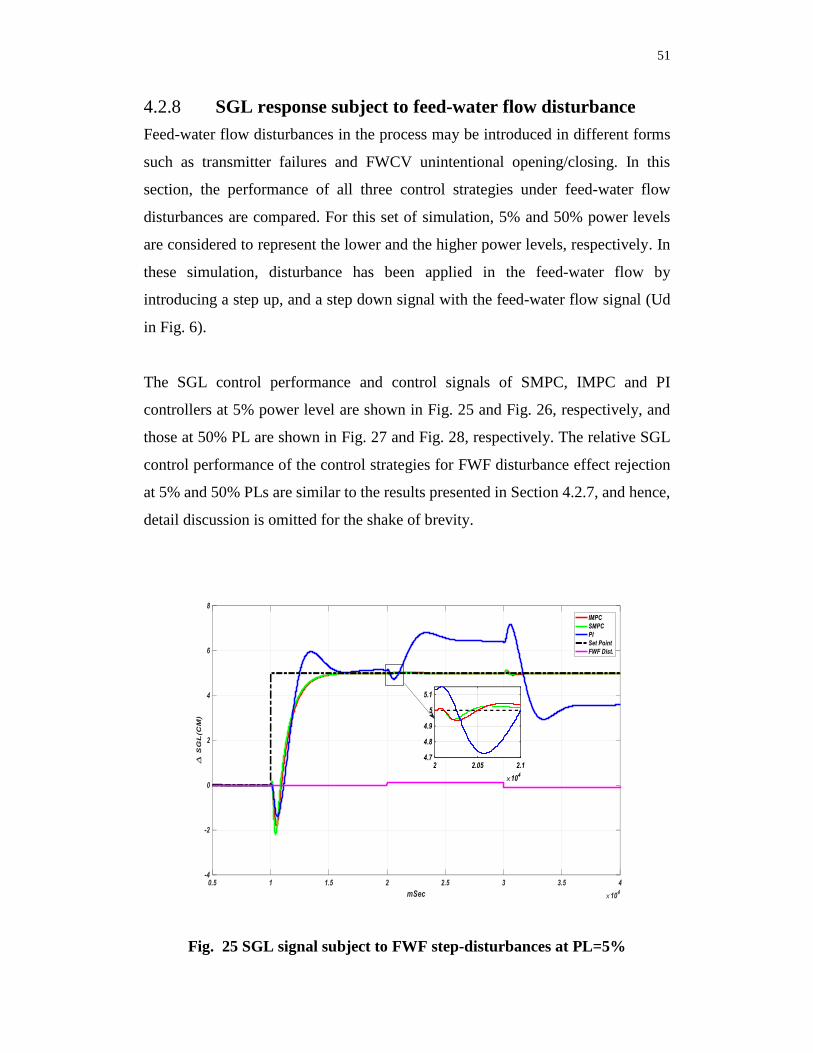
51

4.2.8 SGL response subject to feed-water flow disturbance

Feed-water flow disturbances in the process may be introduced in different forms

such as transmitter failures and FWCV unintentional opening/closing. In this

section, the performance of all three control strategies under feed-water flow

disturbances are compared. For this set of simulation, 5% and 50% power levels

are considered to represent the lower and the higher power levels, respectively. In

these simulation, disturbance has been applied in the feed-water flow by

introducing a step up, and a step down signal with the feed-water flow signal (Ud

in Fig. 6).

The SGL control performance and control signals of SMPC, IMPC and PI

controllers at 5% power level are shown in Fig. 25 and Fig. 26, respectively, and

those at 50% PL are shown in Fig. 27 and Fig. 28, respectively. The relative SGL

control performance of the control strategies for FWF disturbance effect rejection

at 5% and 50% PLs are similar to the results presented in Section 4.2.7, and hence,

detail discussion is omitted for the shake of brevity.

Fig. 25 SGL signal subject to FWF step-disturbances at PL=5%

52

Fig. 26 Control signal subject to FWF step-disturbances at PL=5%

Fig. 27 SGL subject to FWF step-disturbances at PL=50%

53

Fig. 28 Control signal subject to FWF step-disturbances at PL=50%

4.2.9 SGL response subject to random measurement noise in

the FWF

Random noise disturbance in feed-water flow signal can be caused by several

factors such as poor grounding, bad connection, or Electro-Magnetic Interference

(EMI) from a plant environment. In this section the performance of all three control

strategies are compared under random noise-disturbance in the feed-water flow. As

for other simulation under disturbances, 5% and 50% power levels are considered.

Random noise signal has been generated by using Simulink block.

The amplitude for the random signal is selected as 0.3. The noise signal is

introduced in feed-water flow signal (Ud in Fig. 6).

The SGL control performance of SMPC, IMPC and PI controllers at 5% power

levels are shown in Fig. 29, and the respective control signals are shown in Fig. 30.

As shown Fig. 29, random noise has caused about +/- 4% oscillation on the SGL

for the PI controller. The IMPC and the SMPC have been able to handle the noise

effect more resiliently, with approximately +/- 0.4% oscillation on the SGL. The

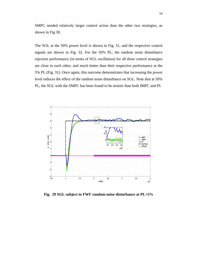
54

SMPC needed relatively larger control action than the other two strategies, as

shown in Fig 30.

The SGL at the 50% power level is shown in Fig. 31, and the respective control

signals are shown in Fig. 32. For the 50% PL, the random noise disturbance

rejection performance (in terms of SGL oscillation) for all three control strategies

are close to each other, and much better than their respective performance at the

5% PL (Fig. 31). Once again, this outcome demonstrates that increasing the power

level reduces the effect of the random noise disturbance on SGL. Note that at 50%

PL, the SGL with the SMPC has been found to be noisier than both IMPC and PI.

Fig. 29 SGL subject to FWF random noise disturbance at PL=5%

55

Fig. 30 Control signal subject to FWF random noise disturbance at PL=5%

Fig. 31 SGL subject to FWF random noise disturbance at PL=50%

56

Fig. 32 Control signal subject to FWF random noise-disturbance at PL=50%

4.3 Summary

The performance of the SMPC and the IMPC based control strategies has been

investigated, and compared with an optimized PI based controller through

computer simulation. The control performance has been evaluated mainly in four

performance measures: i) overshoot, ii) undershoot, iii) settling time, and iv) steady

state errors. Simulation scenarios have been specifically selected in order to

investigate the performance for set point tracking, load following (in step and

programed ramp), load rejection, and to see how they would perform under

disturbances and signal noises in the SF and the feed-water flow.

57

5 Physical Test Results on the PLS

5.1 Background and objectives

Testing control systems in a physical environment is important to verify and

validate the performance and limitations of a control strategy. The quality and

accuracy of the test is dependent on the physical system with respect to actual

system dynamics. In this section, a physical test bench consisting of a mock-up SG

system, referred to as the Plate-Level System (PLS), is used to study the

performance of all three control strategies. The idea has been to investigate the

effectiveness of the control strategies on a realistic system. A subset of the

computer simulation studies has been selected for the PLS test. For the analysis of

the PLS test results, emphasis has been put on the similarity and the differences of

relative performance trends of the PLS test results to that of the corresponding

computer simulation.

5.2 Physical simulation set up

The PLS used to mimic a realistic steam generator level in CIES lab is illustrated

in Fig. 33, and a schematic diagram is shown in Fig. 34. As shown in Fig. 34, the

PLS system consists of a cylindrical tank containing an aluminum plate which can

be controlled vertically by manipulating the position of the valve. This valve

position changes the air flow-rate, which in turn changes the plate level. The plate

moves within an admissible range of 0-20 cm. Plate level “SGL” is measured by a

laser level sensor installed at the top of the tank (Fig. 33), which passes this

information in the form of 4-20 mA output signals to an I/V converter (Fig. 33).

The voltage signal from the converter is then passed to a data acquisition (DAQ)

system. A DT9812 Series DAQ module has been used that supports eight single-

ended analog input channels, two analog output channels (DAC0 and DAC1), eight

fixed digital input lines, and eight fixed digital output lines. This DAQ interfaces

with the MATLAB Data Acquisition (DAQ) subsystem. The FWF and SF signals,

as determined by the control strategy, are passed from the MATLAB DAQ to

DT9812 DAQ over the channels DAC0 and DAC1. These signals then go to the

58

converter V/I. The FWF signal is then fed to the control valve of the PLS (FIG. 34).

The SF is used to set the power level of the PLS.

Laser level sensor

Fig. 33 The Plate Level System (PLS)

A schematic diagram of the plate-level system used for physical simulation is

shown in Fig. 34. [23]

59

unused closed valve

40PSI

20PSI

feed valve

4-20mA

level sensor

+

signal amplifier

PWM

Fe(z)

Fv(z)

vent

plate

digital filter

4-20mA

PWM

ATM

R

4-20mA

FWF SF

Fig. 34 A schematic diagram of the PLS with a digital filter for simulating

non-minimum phase characteristics

5.3 Selection of simulation scenarios

The simulation scenarios for the PLS tests are kept similar to the computer

simulation (discussed in Section 4.2), so that meaningful comparisons can be made.

The results of the simulation are discussed in the following.

Note that the PLS cannot be pulled-down by the feed-air valve during the set point

step-up change, and hence, undershoot performance subject to set point step-up

change cannot be measured for PLS test studies. Therefore, undershoot measure

during set point step-up change has been disregarded for all test results presented

in this section. Furthermore, the PLS tests with SF disturbance have not been

performed, as the SF valve on the PLS is not physically integrated with the process.

Furthermore, only random noise disturbance in the FWF has been considered for

physical tests.

60

5.3.1 Step response

The step responses of the control strategies on the PLS are investigated at 5%, 15%,

and 100% power levels. These power levels are selected to reflect the performance

evaluation of the control strategies at low power levels and a high power level. The

results are shown in Fig. 35 to Fig. 40. As in the computer simulation, the unit of

SGL (change in SGL) is given in centimeters, and the control signal, which is the

FWF rate, is given in kg/s. The main observations from this set of simulation have

been summarized in Table 7, along with a discussion, to be presented later in this

section. The simulation time has been set to 3.5x10^4. The longer simulation time

(than the respective computer simulation) has been used to ensure appropriate

settling time (+/- 2% SGL) for all of the control strategies. The steady state errors

reported in this section are the error at the end of the simulation times.

The SGL performance of SMPC, IMPC and PI controllers at 5% power level are

shown in Fig. 35, and the respective control signals are shown in Fig. 36. As shown

in Fig. 35 (and Table 7), only a little overshoot has been observed for the IMPC

and the SMPC schemes at this PL (1.7% and 4.56%, respectively). There were zero

overshoots with these controllers in the computer simulation at 5% PL (Table 6).

However, the overshoot with the PI on the PLS is about 33% (computer simulation

for PI has been 19.1%). This may be due to the saturation of the PI control signals,

as shown in Fig. 36.

In summary, the relative SGL performance trend of the controllers on the PLS, in

terms of overshoot, is reasonably close to that of the computer simulation.

The steady state errors on the PLS for IMPC, SMPC and PI in Fig. 35 have been

0.5%, 0.3%, and 3.25%, respectively (Table 7). IMPC and SMPC have zero steady

state errors in computer simulation (Table 6). And therefore, relative SGL

performance trend of the controllers on the PLS and the computer simulation, in

terms of steady state error, is also fairly close. The PI needed relatively larger

control action than the other two strategies, as shown in Fig 36.

61

At 5% power level, both SGL and control signals are found to be noisy as shown

in Fig. 36. And hence, the settling time cannot be clearly identified. These noises

are relatively more as compared to the corresponding computer simulation.

However, this can be expected due to the physical nature of the test, and the

characteristics of the PLS. Furthermore, although the PLS closely mimic the Irving

model, some model mismatch can be expected, which may lead to a variation in the

performance of the MPC based control strategies. It is noted that such noises in the

SGL and the control signals have been observed in all test cases in low power levels

due to the possible reasons discussed above.

Fig. 35 SGL of the PLS at PL=5%

62

Fig. 36 Control signal to the PLS at PL=5%

The SGL performance of SMPC, IMPC and PI controllers at 15% power level in

shown in Fig. 37, and the respective control signals are shown in Fig. 38. Visual

inspection of Fig. 37 clearly reveals that SGL by the SMPC and the PI have suffered

from oscillations. This is different from the corresponding computer simulation, as

no oscillation has been observed (see Fig. 7). This may have occurred due to model

mismatch. The IMPC has shown no SGL oscillation on PLS, possibly indicating

that the IMPC is more robust in terms of model mismatch.

The PI has shown a larger overshoot of 32.23% (see Table 7) than the computer

simulation (11.08%, see Table 6). The SMPC has shown 13.33%% overshoot,

whereas, the IMPC has only a little overshoot (3.33%). Both IMPC and SMPC

overshoots were zero in the computer simulation. Therefore, the IMPC has again

shown better capability in terms of overshoot.

The steady state errors on the PLS, for all controllers, are comparable to that of the

computer simulation (see Table 6 and Table 7). For the settling time, all control

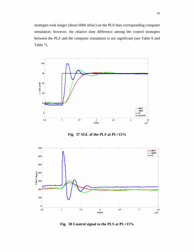
63

strategies took longer (about 6000 mSec) on the PLS than corresponding computer

simulation; however, the relative time difference among the control strategies

between the PLS and the computer simulation is not significant (see Table 6 and

Table 7).

Fig. 37 SGL of the PLS at PL=15%

Fig. 38 Control signal to the PLS at PL=15%

64

The SGL performance of SMPC, IMPC and PI controllers at 100% power level

are shown in Fig. 39, and the respective control signals are shown in Fig. 40.

From Fig. 39, the SGL performance at 100% power can be seen as similar to that

of the PLS simulation at 15% (Fig. 37).

Fig. 39 SGL of the PLS at PL=100%

Fig. 40 Control signal to the PLS at PL=100%

65

The performance of the three control strategies for the physical simulation is

summarized in Table 7. From this table, it can be seen that the relative performance

trends of the control strategies are close to those in the computer simulation, except

for the settling times, where the PLS tests have required larger settling times for all

control strategies (see Tables 6 and 7). Furthermore, overshoots can be seen in both

MPC based approaches for PLS tests, although the overshoot is minimal for the

IMPC scheme. Steady state error for all three control strategies on the PLS are also

close to that of the computer simulation.

Table 7 Performance of IMPC, SMPC and PI strategies on the PLS

%PL

Over Shoot (%) Settling Time (mSec) Steady State Error (%)

at simulation end time

IMPC SMPC PI IMPC SMPC PI IMPC SMPC PI

5 1.7 4.56 33.33 na na na 0 0 3.25

15 3.33 13.33 32.23 6760 6600 7050 0 1.17 2

100 1.3 10.66 31.02 7460 4000 5200 0 0 0

5.3.2 SGL response subject to changes in reactor power level

in step

The same as in the computer simulation presented in Section 4.2.5, this PLS test

has been done in order to study the performance of the control strategies when

reactor power levels are changed from 5% to 22%. From 5% to 19%, PL has been

increased by a step of 2%; and then, the PL is increased by 3% to arrive at 22%.

The results are shown in Fig. 41 and Fig. 42 (the SGL and the control signals,

respectively).

It can be seen in Fig. 41 that the load following capability of the IMPC and the

SMPC controllers are better than the PI, and close to each other. However, their

performance is a little noisy compared to the corresponding computer simulation

(Fig. 17), most likely due to the model mismatch. Comparing Fig. 41 and Fig. 17,

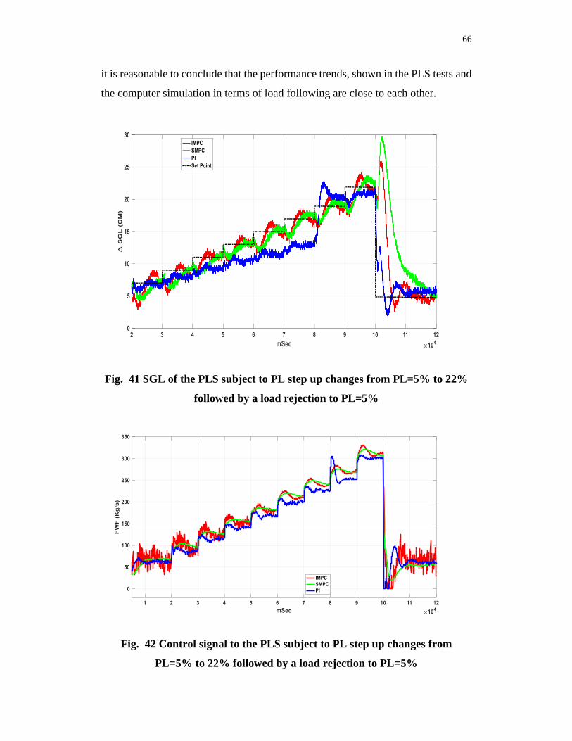
66

it is reasonable to conclude that the performance trends, shown in the PLS tests and

the computer simulation in terms of load following are close to each other.

Fig. 41 SGL of the PLS subject to PL step up changes from PL=5% to 22%

followed by a load rejection to PL=5%

Fig. 42 Control signal to the PLS subject to PL step up changes from

PL=5% to 22% followed by a load rejection to PL=5%

67

5.3.3 SGL response subject to changes in reactor power level in ramp

For this PLS test, the reactor power is increased continuously from 5% to 100%

(ramp up), and then reduced to 22% (load rejection). The results are shown in Fig.

43 and Fig. 44 (SGL and control signal, respectively). In this simulation, the set

point tracking performance of all three control strategies have shown little

degradation compared to their computer simulation counterparts (Fig. 19). One of

the major reasons is the possible model mismatch.

The SMPC has the best performance in terms of set point tracking and load

following, with IMPC a close second. The IMPC, however, has the least

undershoots, and also the least settling time (after load rejection). Relatively much

larger overshoot/undershoot and settling time can be noted for PI.

Note that the spikes in the control signal in PI are due to the switch of the controller

to a different power level. This can be avoided by using bump less PI as shown in

corresponding computer simulation (Fig. 20).

Fig. 43 SGL of the PLS for PL ramp up changes from PL=5% to 80%

followed by load rejection to PL=10%

68

Fig. 44 Control signal to the PLS for PL ramp up changes from PL=5% to

80% followed by load rejection to PL=10%

5.3.4 SGL response subject to random noise in the FWF

measurements

This section presents the performance of control strategies subject to random noise

in the FWF measurements. For this set of the PLS tests, 5% and 50% power levels

are considered, as in the computer simulation.

The results at 5% PL are shown in Fig. 45 and Fig. 46 .. Little more noises and

oscillations in the SGL can be seen for all control strategies in Fig. 45, as compared

to the respective computer simulation, Fig. 29 (possibly, due to model mismatch).

The performance in terms of noise effect rejection of all control strategies are

comparable.

69

Fig. 45 SGL of the PLS subject to FWF random noise at PL 5%

Fig. 46 Control signal to the PLS subject to FWF random noise at PL 5%

70

The results at 50% PL are shown in Fig. 47 and Fig. 48. At this power level, the

noise effect rejection performance of all control strategies are comparable, and

similar to that of the respective computer simulation (Fig. 31).

Fig. 47 SGL of the PLS subject to FWF random noise at PL 50%

Fig. 48 Control signal to the PLS subject to FWF random noise at PL 50%

71

5.4 Summary

The performance of the MPC based controllers has been evaluated through a set of

physical tests on the PLS. The performance measures of the control strategies are

evaluated in terms of set point tracking, load following in steps and programed

ramp, load rejection, and flow disturbance and signal noise rejection capabilities.

The performance measures of the control strategies on the PLS are compared with

the computer simulation results.

72

6 Conclusions and Future Work

6.1 Contributions

The performance of the MPC based strategies to control the SGL in NPPs have

been evaluated. In-depth studies have been performed to better understand the

capability of the MPC based control schemes to deal with the challenges in the SGL

control in NPPs over the full power range. Performance has been evaluated with

respect to all operating and transient conditions of a SG in a NPP.

These evaluations have been carried out using a linearized steam generator dynamic

model. The MPC controllers used are based on existing methodologies.

Furthermore, any potential performance improvement through fine-tuning of some

of the control parameters (based on the dynamic characteristics of the SGL) has

also been investigated.

For performance evaluation, two versions of the MPC strategy, the SMPC and the

IMPC, have been designed and simulated. The SMPC scheme is based on existing

MPC methodologies. The IMPC has been examined for potential performance

improvement over SMPC by selecting appropriate values in the weight matrix of

the objective function.

The Irving model has been used as the underlying dynamic model of the SG in this

study. This model has been linearized over the entire power range. Since the Irving

model changes with power levels, power level dependent SGL parameters of the

SGL have been designed. Power level dependent control parameters have been

designed through minimizing an appropriate cost function that has been selected.

Furthermore, for the IMPC, a simple strategy has been presented to compute the

weights in the IMPCQ matrix. The IMPCQ matrix has been used to manipulate the

control signals in order to improve the SGL performance of the MPC based

strategies.

73

Performance of the SMPC and the IMPC has been evaluated, and compared with

an optimized PI controller. The performance has been evaluated through computer

simulation, and also through a set of physical tests on the PLS (the mock-up steam

generator level system). Performance evaluations have been done in terms of i) set

point tracking, ii) load-following, transient responses, and iii) effectiveness under

flow disturbances and signal noise.

6.2 Discussions and conclusions

In the computer simulation, the SMPC and the IMPC schemes have shown zero

overshoot and steady-state errors over all power levels, for the SGL subject to the

step response. In the PLS tests, the IMPC scheme has shown zero steady-state errors

and close-to-zero overshoots, while the SMPC has shown a little more overshoots

(others are close-to-zero). There are no significant differences between the settling

times among the control strategies in most cases.

With respect to the reactor power changes in steps and in ramps, as well as with

respect to the load rejections, the computer simulation and the PLS test results have

indicated similar relative performance trends for the control strategies. The IMPC

method has consistently shown improved capability for set point tracking in all

these simulation and tests, although the improvements on the PLS are marginal.

Furthermore, both the SMPC and the IMPC have shown similar capabilities for

rejecting the effect of flow disturbances in the computer simulation, as well as in

the PLS tests.

Based on all these observations, it can be concluded that the IMPC has a strong

potential to become a feasible methodology for the SGL control in NPPs to cover

all operating conditions over all power levels.

74

6.3 Future work

The PLS simulation has provided some insights on the performance of the MPC

based control strategies with real systems. However, it is not a real SG. More

research needs to be done in order to evaluate the performance of the SMPC and

the IMPC in a more realistic set up of a SG in a NPP.

Furthermore, the IMPC scheme that has been evaluated in this study is based on

certain values for the elements of the weight matrix IMPCQ . These values have been

computed by using a simple heuristic method. Clearly, the IMPCQ matrix selected in

this study are not optimal. Therefore, more research needs to be done to develop

effective algorithms and methodology that can compute optimal values for these

elements for all power levels.

75

References

[1] A. Osgouee and J. Jiang, “Robust Nonlinear Method for Steam Generator

Level Control,” Nuclear Technology, Vol. 181, 3, pp. 493-506, 2013.

[2] L. Bonavigo and M. D. Salve, “Issues for Nuclear Power Plants Steam

Generators”, Book Chapter, DOI: 10.5772/14853, InTech, 2011

[3] E. Irving, C. Miossec, and J. Tassart, “Towards efficient full automatic

operation of the PWR steam generator with water level adaptive control” In

Proceedings of the International Conference on Boiler Dynamics and Control

in Nuclear Power Stations, pp. 309-329, 1980.

[4] S.K. Menon and A.G. Parlos, “Gain-Scheduled Nonlinear Control of U-Tube

Steam Generator Water Level” Nuclear and Science and Engineering: 111,

pp. 294-308, 1992.

[5] K.J. Astrom and R.D. Bell, “Drum-boiler dynamics,” (Report TFRT; Vol.

7577). Department of Automatic Control, Lund Institute of Technology

(LTH), 1998.

[6] M.K. Kim, M.H. Shin and M.J. Chung, “A gain–scheduled L2 control to

nuclear steam generator SGL,” Ann. of Nucl. Energy 26, 905–16, 1999.

[7] M.V. Kothare, B. Mettler, M. Morari, P. Bendotti, “Level control in the steam

generator of a nuclear power plant”, IEEE Transactions on Control Systems

Technology, Vol. 8, 1, pp. 55-69, Jan 2000.

[8] T. Iijima, Y. Nakajima and Y. Nishiwaki, “Application of fuzzy logic control

system for reactor feed–water control,” Fuzzy Sets and Systems, Vol, 74, pp.

61–72, 1995.

[9] B.H. Cho and H.C. No, “Design of stability–guaranteed neurofuzzy logic

controller for nuclear steam generators,” Nucl. Eng. and Design 166 17–29,

1996.

[10] B.H. Cho and H.C. No, “Design of stability and performance robust fuzzy

logic gain scheduler for nuclear steam generators,” IEEE Trans. on Nuclear

Science, Vol. 44, pp. 1431–41, 1996.

76

[11] M.G. Na, “Design of genetic fuzzy controller for the nuclear steam generator

SGL control,” IEEE Trans. on Nucl. Science, Vol. 45, pp. 2261–71, 1998.

[12] M.K. Kim, M.H. Shin and M.J. Chung, “A gain–scheduled L2 control to

nuclear steam generator SGL,” Ann. of Nucl. Energy, Vol. 26, pp. 905–16,

1999.

[13] A.G. Parlos, S. Parthasarathy and A.F. Atiya, “Neuro–predictive process

control using on-line controller adaptation,” IEEE Trans. on Con. Sys.

Technology, Vol. 9, pp. 741–55, 2001.

[14] M.G. Na, Y.R. Sim, and Y.J. Lee, “Design of an adaptive predictive

controller for steam generators,” IEEE Trans. on Nucl. Science, Vol. 50, pp.

186–93, 2003.

[15] M.V. Kothare, B. Mettler, M. Morari, P. Bendotti and C.M. Falinower,

“Level control in the steam generator of a nuclear power plant,” IEEE Trans.

on Contr. Sys. Technology, Vol. 8, pp. 55–69, 2000.

[16] H. Kwakernaak and R. Sivan, “Linear Optimal Control Systems,” Wiley-

Interscience, 1972.

[17] Man Gyun Na, “MPC-Based Auto-tuned PID Controller for the Steam

Generator Water Level”, Proceedings of the Korean Nuclear Society Spring

Meeting Cheju, Korea, May 2001.

[18] Le Wei, Fang Fang “H∞-based LQR water level control for nuclear u-tube

steam generators”, 25th Chinese Control and Decision Conference (CCDC),

2013.

[19] J. J. Sohn and P. H. Seong, “A steam generator model identification and

robust H∞ controller design with ν-gap metric for a feedwater control

system”, Annals of Nuclear Energy, vol. 37, no. 2, pp. 180–195, Feb. 2010.

[20] EPRI, Model Predictive Control – Concepts, Design and Tuning, December

2015.

[21] L. Wang, Model Predictive Control System Design and Implementation

Using MATLAB, Springer, 2009.

77

[22] W. Hur, P. Seong, “Optimal Sampling Period of the Digital Control System

for the Nuclear Power Plant Steam Generator Water Level Control”, Journal

of Korean Nuclear Society, Vol 27(1), pp. 8-17, 1995.

[23] Drew J. Rankin and Jin Jiang, “Analytically Compensated SGLC Test

Facility”, Proceedings of NPIC& HMIT, 2015.

[24] M. Akkawi and J.Jiang, “An Inverse Control-based Set-point Function for

Steam Generator Level Control in Nuclear Power Plants,” IEEE Trans. on

Nuclear Science , 58(6), pp. 3291-3304 Nov. 2011

[25] I. Horowitz and Y. K. Liao, “Limitations of non-minimum-phase feedback

systems,” International Journal of Control, Vol. 40, I-5, pp. 1003-1013, 1984.

[26] R. Findeisen, and F. Allgower, “An Introduction to Nonlinear Model

Predictive Control,” Proceedings of 21st Benelux Meeting on Systems and

Control, 2002.

[27] A. Feliachi and L.A. Belbelidia, “Suboptimal level controller for steam

generators in pressurized water reactors,” IEEE Trans. on Energy Conversion

3, pp. 278–84, 1988.

[28] J.I. Choi, J.E. Meyer and D. Lanning, “Automatic controller for steam

generator SGL during low power operation,” Nucl. Eng. and Design 117, pp.

244–63, 1989.

[29] T. Iijima, Y. Nakajima and Y. Nishiwaki, “Application of fuzzy logic control

system for reactor feed–water control,” Fuzzy Sets and Systems 74, pp. 61–

72, 1995.

[30] G. Ablay, “Steam Generator Level Control with an Observer-Based

Algebraic Approach”, Proceedings of Electrical and Electronics Engineering

(ELECO), Nov. 2013.

[31] W.Tan, Water level control for a nuclear steam generator. Nuclear

Engineering and Design 241, pp. 1873–1880, 2011.

[32] N. Bonavita, J. Caserza, R. Martini, “Tuning loop: control performance and

diagnostics”, ABB Process Solutions & Services, 2006.

[33] A. Osgouee, J. Jiang, ‘Robust model-based steam generator level control in

Nuclear Power Plant,’ Proc. of 28th Canadian Nuclear Society Conference &

78

31st CNS/CAN Student Conference, St. John, New Brunswick, June 3-6,

2007.

79

CURRICULUM VITAE (CV)

Work History

2000 - Present, Senior Technical Engineer at Ontario Power Generation

1985 - 2000, Senior I&C Engineer at Tavanir, Iran

Education

M.E.Sc from the Department of Electrical Engineering-Electronic at the

Amirkabir, University of Technology, Tehran, Iran in 1989

B.E.Sc from the Department of Electrical Engineering-Control at the Sharif

University of Technology, Tehran, Iran in 1982

Research interest

Design and upgrade of control systems, and optimal controller tuning.

Design of advanced model predictive control systems for steam generator level.

Teaching experience

1989 – 1999: Taught industrial control, control systems and electronics as a part

time instructor at the Tabriz University in Iran.

Awards

1986 – 1999: Recipient of a number of gold medals from various seminars,

including the International Power System Conference, in Iran.

Conference presentations

Presented papers at CNS, and several International Conferences.

80

Publications

[1] A. Osgouee, J. Jiang, “Robust Nonlinear Method for Steam Generator Level

Control,” Nuclear Technology / Volume 181 / Number 3 / March 2013 / Pages

493-506, 2013.

[2] A. Osgouee, “Upgrading steam generator level control strategy at nuclear

power plants,” The 5th CNS International Steam Generator Conference, Toronto,

2006.

[3] A. Osgouee, “Steam Generator level control at nuclear power plants,” 28th

Annual Conference of the Canadian Nuclear Society, Saint John, New Brunswick,

June 2007.