Model Predictive Fuzzy Control of a Steam Boiler · Abstract . This thesis is devoted to apply a...
116
Treball Fi de Màster Master’s degree in Automàtic and Robotics Model Predictive Fuzzy Control of a Steam Boiler MEMÒRIA Autor: Michael Alejandro Blanco Baptista Director/s: Vicenç Puig Cayuela Convocatòria: Setembre 2016 Escola Tècnica Superior d’Enginyeria Industrial de Barcelona
Transcript of Model Predictive Fuzzy Control of a Steam Boiler · Abstract . This thesis is devoted to apply a...

Treball Fi de Màster Master’s degree in
Automàtic and Robotics
Model Predictive Fuzzy Control of a Steam Boiler
MEMÒRIA
Autor: Michael Alejandro Blanco Baptista
Director/s: Vicenç Puig Cayuela
Convocatòria: Setembre 2016
Escola Tècnica Superior d’Enginyeria Industrial de Barcelona


Abstract
This thesis is devoted to apply a Model Predictive Fuzzy Controller (MPC and Takagi-Sugeno) to a specific Steam Boiler Plant. This is a very common problem in control. The considered plant is based on the descriptions obtained from the data of a referenced boiler in the combined cycle plant as Abbot in Champaign, Illinois. The idea is to take all the useful data from the boiler according to its performance and capability in different operation points in order to model the most accurate plant for control.
The considered case study is based in a modification of a model proposed by Pellegrinetti and Bentsman in 1996, considering to be tested under the demands of the Control Engineering Association (CEA). The system is Multi-Input and Multi-Output (MIMO), where each controlled output has a specific weight in order to measure the performance. The objective is to minimize cost index but also make it operative and robust for a wide range of variables, discovering the limits of the plant and its behaviour.
The model is supposed to manage real data and was constructed under real physical descriptions. However, this model is not a white box, so the analysis and development of the model to be used with the MPC strategy have to be identified to continue with the evaluation of the controlled plant. There are some physical variables that have to be taken into account (Drum Pressure, Excess of Oxygen, Water Level, Water Flow, Fuel Flow, Air Flow and Steam Demand) to know if these variables and other parameters are evolving in the correct way and satisfy the logic of the mass and energy balances in the system.
After measuring and analysing the data, the model is validated testing it for different values of steam demands. The controller is tuned for every one of the considered demands. Once tuned, the controller computes the manipulated variables receiving information from the controlled ones, including their references. Finally, the resulting controller is a combination of a set of local controllers using the Takagi-Sugeno approach using the steam demand setpoint as scheduling variable. To apply this approach, a set of local models approximating the non-linear boiler behaviour around a set of steam demand set-points are obtained and then their a fused using the Takagi-Sugeno approach to approximate any unknown steam demand located in the valid range of values.
Keywords: MPC, Identification, Fuzzy, Modelling, Steam Boiler, Industrial, CEA, Takagi-Sugeno.
iii

iv

Acknowledgments I want to express my gratitude to my advisor, Dr Vicenç Puig, for his support, advices and patience during the realization of all this project. This was an important way to learn and a good end for this stage of my life. To my colleagues, they were as much important as the professors in this journey. To my friends, the most valuable thing I found in these couple of years. As we said sometimes, you are my family out of our borders. To my family, for they support and sacrifice. All of you motivate me all the days to get up and look for a promissory future, I will see you soon always.
Michael Blanco Barcelona, September 2016
v


Notation Throughout the thesis, scalars are denoted with lower case letters (e.g., a, b, _, _, .
. .), vectors are denoted with bold lower case letters (e.g., a, b, . . .), matrices are denoted with bold upper case letters (e.g., A, B,. . .), and sets are denoted with upper case blackboard bold letters (e.g., , ,. . .) for constraint sets. If not otherwise noted, all vectors are column vectors. Sets, Spaces and Set Operators set of real numbers +0 set of non-negative real numbers including zero
n space of n-dimensional (column) vectors with real entries
n m× space of n by m matrices with real entries set of natural numbers (non-negative integers), + := \{0} kj set of consecutive non-negative integers j, . . . , k (⊂) ⊆ (strict) subset \ set minus × Cartesian product, X × Y = {(x, y) | x ∈ X, y ∈ Y} Model Theory qf fuel flow rate qa air flow rate qfw water flow rate QFCF maximum fuel flow rate QACA maximum air flow rate QCFW maximum water flow rate CPi constants for modelled equation O2 remaining oxygen FAR air to fuel mass ratio AIRO2 rate of oxygen in the air TAIR time constant for air flow VW Volume of water inside the drum VT Total volume of the drum xi states ui inputs yi outputs cij constants for the model Systems and Control Theory nx number of states, nx ∈ +
vii

nu number of inputs, nu ∈ +
nd number of disturbances, nd ∈ +
x state vector, x ∈ nx
u control input vector, u ∈ nu
d disturbance vector, d ∈ nd
X set of admissible states, X ⊂ nx
U set of admissible control inputs, U ⊂ nu
MPC Theory N prediction horizon J cost function xk states in the instant k uk inputs in the instant k xN states in the instant N k current control interval p prediction horizon (number of intervals) ny Number of plant input variables
zk QP decision ( | ) ( 1| ) ( 1| )T T T Tkz u k k u k k u k p k = + + −
( | )y k i k+ Predictive value of jth plant output at ith prediction horizon step
( | )r k i k+ Reference value for jth plant output at ith prediction horizon step yjs Scale factor for jth plant output
,yi jw Tuning weight for jth plant output at ith prediction horizon step
nu Number of manipulated variables
, arg ( | )j t etu k i k+ Target value for jth MV at ith prediction horizon step ujs Scale factor for jth plant MV
,ui jw Tuning weight for jth plant MV at ith prediction horizon step
,u
i jw∆ Tuning weight for jth plant MV rate at ith prediction horizon step
ke slack variable at control interval k
ρ constraint violation penalty weight
Takagi-Sugeno Theory
ijM the fuzzy set
r number of model rules x(t) state vector u(t) input vector y(t) output vector
,, ,i i i iA B C D functions of state
z(t) premise variables
viii

w weights h weights proportion IF-THEN classic conditions Thermodynamics Basic Theory ṁi input mass flow ṁo input mass flow U internal energy of a system Q heat that is transferred to a system W work needed by a system in a process P pressure PM molecular weight V volume R constant for the ideal gases n moles T temperature
ix

x

Contents ABSTRACT ................................................................................... III
ACKNOWLEDGMENTS .................................................................. V
NOTATION ................................................................................. VII
CONTENTS .................................................................................. XI
LIST OF TABLES ....................................................................... XV
LIST OF FIGURES .................................................................... XVII
1 INTRODUCTION ..................................................................... 1
1.1 MOTIVATION .................................................................................. 1
1.2 THESIS OBJECTIVES AND SCOPE ..................................................... 3
1.2.1 Scope of Research ................................................................ 4
1.3 OUTLINE OF THE THESIS ................................................................ 4
2 BACKGROUND ........................................................................ 7
2.1 INDUSTRIAL STEAM BOILERS .......................................................... 7
2.2 THERMODYNAMIC BASIS ................................................................10
2.3 MPC CONTROLLERS ......................................................................12
2.3.1 Considering Model Based Predictive Control...................12
2.3.2 General Considerations.......................................................14
3 MODELLING A STEAM BOILER ........................................... 17
3.1 GENERAL DESCRIPTION OF THE CASE STUDY ................................17
3.1.1 Analysed Boiler Models ......................................................17
3.1.2 Known Conditions of the Model .........................................23
3.1.3 Encrypted Model .................................................................24
3.2 IDENTIFICATION OF THE PLANT.....................................................28
3.3 VARIATION OF THE MEASURED DISTURBANCE ................................33
xi

4 MPC OF THE BOILER SYSTEM ............................................ 39
4.1 MODEL-BASED PREDICTIVE CONTROLLER .....................................39
4.1.1 Nonlinear MPC considerations ...........................................43
4.1.2 MPC Toolbox .......................................................................43
4.1.3 Constraints ..........................................................................46
4.1.4 Weights ................................................................................50
4.2 NONLINEAR CONTROLLER APPROXIMATIONS .................................52
4.2.1 Considered Techniques ........................................................53
4.2.2 Takagi-Sugeno ......................................................................54
4.3 IMPLEMENTATION ON PLANT .........................................................60
4.3.1 MPC Block ...........................................................................61
4.3.2 Tuning ...................................................................................63
5 RESULTS ............................................................................... 69
5.1 BOILER PLANT IDENTIFICATION .....................................................69
5.2 SYSTEM EVALUATION STUDY.........................................................74
5.3 BOILER PLANT CONTROL ..............................................................80
6 BUDGET AND IMPACT STUDY ............................................ 85
6.1 BUDGET STUDY .............................................................................85
6.1.1 Hardware resources ............................................................85
6.1.2 Software resources .............................................................86
6.1.3 Human resources ..................................................................86
6.1.4 General expenses .................................................................87
6.1.5 Total Cost ...........................................................................87
6.2 IMPACT STUDY ..............................................................................87
6.2.1 Economic impact ...................................................................88
6.2.2 Environmental impact .........................................................88
7 CONCLUDING REMARKS ..................................................... 89
7.1 CONCLUSIONS ................................................................................89
7.2 CONTRIBUTIONS ............................................................................90
xii

7.3 DIRECTIONS OF FUTURE RESEARCH ..............................................90
BIBLIOGRAPHY ........................................................................... 91
xiii


List of tables
Table 1. Initial conditions of the Steam Boiler ..................................................... 25
Table 2. Parametrizations of the system components (Mathworks, 2016) ............. 30
Table 3. Input signal properties ........................................................................... 46
Table 4. Output signal properties ......................................................................... 46
Table 5. Constraint characteristics by default (Mathworks, 2016) ........................ 47
Table 6. Constraints configuration of the model ................................................... 48
Table 7. Set point values of the plant .................................................................. 51
Table 8. Tuned Weights to control the model ...................................................... 51
Table 9. Difference of parameter in the matrix A of identification ....................... 70
Table 10. Difference of parameter in the matrix B of identification ...................... 71
Table 11. Difference of parameter in the matrix C of identification ...................... 72
Table 12. Cost associated to hardware resources .................................................. 85
Table 13. Cost associated to hardware resources .................................................. 86
Table 14. Total Costs ........................................................................................... 87
xv

xvi

List of figures
Figure 1. Heat of 1 Kg of water at normal pressure (1 atm). The phase I is solid, the
phase II is liquid and the phase III is gas. (Reina, 2016) ............................................... 9
Figure 2. Battery of Boilers in a Combined Cycle Plant. The innovative way of heat
optimization. (Wärtsilä, 2016) ...................................................................................... 9
Figure 3. Technical possibilities vs expectations of control techniques (Bordons,
2000) ........................................................................................................................... 13
Figure 4. The model structure used in the MPC controller (Mathworks, 2016) .... 15
Figure 5. Industrial Steam Generator Plant (Pellegrinetti & Bentsman, 1996). .... 18
Figure 6. MIMO block of the boiler and it internal structure (Comité Español de
Automática, 2016) ....................................................................................................... 25
Figure 7. Steam demand pattern .......................................................................... 26
Figure 8. Reference and measured outputs of the steam boiler case study ............ 26
Figure 9. Input measured variables in the steam boiler case study ....................... 27
Figure 10. Types of Models (Mathworks, 2016) .................................................... 29
Figure 11. Conditions for the identification of State Space models ....................... 31
Figure 12. Identified outputs of the plant using state space method and infinite
horizon ........................................................................................................................ 32
Figure 13. Identified outputs of the plant by using the state-space method and one-
step ahead prediction horizon ...................................................................................... 33
Figure 14. Variation of the Measured Disturbance (Steam Demand) .................... 34
Figure 15. Outputs depending on the steam demand variation............................. 34
xvii

Figure 16. Inputs depending on the steam demand variation ............................... 36
Figure 17. Outputs of the plant with a model identified in state-space, infinite
prediction horizon and at steam demand at 37% ......................................................... 37
Figure 18. Outputs of the plant using a state-space method, one step ahead horizon
and demand 37% ......................................................................................................... 38
Figure 19. Comparison of workflows of the system and the Model Predictive
Controller Toolbox ...................................................................................................... 45
Figure 20. Inputs of the model with constraints ................................................... 49
Figure 21. Outputs of the model with constraints ................................................ 49
Figure 22. Model inputs after tuning the weights ................................................. 51
Figure 23. Model outputs after tuning the weights ............................................... 52
Figure 24. Model Based Fuzzy control design (Tanaka & Wang, 2001) ................ 55
Figure 25. Takagi-Sugeno Decision rules .............................................................. 56
Figure 26. Takagi-Sugeno with PDC based on two controllers ............................. 60
Figure 27. MPC Block in the simulator ................................................................ 61
Figure 28. MPC outputs implemented on plant without tune .............................. 61
Figure 29. MPC inputs implemented on plant without tune ................................ 62
Figure 30. Input in the tuned MPC ...................................................................... 64
Figure 31. Outputs of the tuned variables ............................................................ 65
Figure 32. Inputs obtained using the Takagi Sugeno’s technique .......................... 65
Figure 33. Outputs obtained using the Takagi-Sugeno’s technique ....................... 66
Figure 34. Steam produced using the -Sugeno’s technique .................................... 66
Figure 35. Simulation for the mass balance analysis ............................................. 76
Figure 36. Inputs of the system for selected MPCs ............................................... 80
xviii

Figure 37. Outputs of the system for selected MPCs ............................................ 81
Figure 38. Comparison between a linear and fuzzy MPC application. Inputs ....... 82
Figure 39. Comparison between a linear and fuzzy MPC application. Outputs .... 83
xix


Chapter 1
1 Introduction
1.1 Motivation
Global warming has been a major concern of the world community, since control of
the quality of life levels of mankind could be kept. From the years 70, the emissions of
CO2 have been increasing leading to the effect which nowadays is known as the
greenhouse effect.
It has been as influential during this period time, which is considered that there is
no reverse action in the increase of the temperature of the earth over the next 100 years.
The only option that remains is to reduce the damage that may cause the pollution
generated by the society. The role of all the governments and over all the developed
countries is to apply some policies to reach the objective of keep the increase of
temperature in the Earth below 2 Kelvin at 2100.
In order to reach this objective, they met for the first time in Japan in 1997, around
12% of the countries of the world to establish a treaty that would begin in the new
century and that would mark tendency in the reduction of emissions. This treaty did not
count on the participation and support of great world-wide powers. It was not until the
last year where the world-wide leaders of 172 countries met to talk on the gravity of the
subject and to reach political, economic and social agreements to protect the atmosphere.
1

In 2015, during the summit of the climate of Paris different agreements were reached
to the established objective of reducing emission. First, it was accepted that the energy
is a necessary source for the development, and working on this base and the limits and
possible economic and social incentives for all, the organisms studied the application to
get into this goal.
So, based on the energy production and usage could not be stopped around the
world, the idea is to create new ways of renewable energy or to optimize the classic
production processes. On the one hand, there is the increase of new renewable resources
as solar energy, wind energy, sea energy, electrical energy, nuclear energy, the use of
molecules with high stored energy, etc. And then we have the classic combustion energy,
it was and still is the energy for excellence when the industries think about easy, quick,
efficient and cheap generation.
There will be a quite a more years with this type of energy as the first used in the
world. The technology of the new renewable energies is still not available for most of the
countries presenting some limitations for a lot of industrial sectors. So, the best thing to
do now is to optimize the use of combustion, a big step for this it was to reduce the use
of carbon and increase in the same way the use of fuel but there is still a lot of space for
improvement to work on.
The fuel is one of the main materials to produce energy in any plant. This energy
can be heat, steam, electricity and others. But, it is well known that the efficiency of this
way of producing energy is not the best. In order to get better results, some systems have
been developed to take advantage of this heat and energy that is lost in some phases of
the process.
A Combined Cycle Plant (CCP) is the most recent technology which is based on
some pressure stations with several boilers and several chambers where steam can be
produced at different pressures and temperatures, including clean water as refrigerant
and air to generate electrical energy. At the end, the principle of a CCP relies on the
classic steam boiler, with improved and optimized efficiency.
2

This thesis is based on the optimization of the use of the energy produced by a real
steam boiler which can be operated on a wide range of demand, with fixed pressure and
temperatures. This can be just an example of how the processes can be optimized through
the new control techniques, assuring to be operationally correct and safe. This
optimization help in the reduction of wasted energy and is one of the main branches of
the environmental agreement.
1.2 Thesis Objectives and Scope
First, the main and specific objectives to be achieved during this thesis are presented.
Then, the scope of the research to be developed to achieve these objectives is described
Focusing on the control of an industrial steam boiler, which is a popular control
problem and is looking continuously for improvements, the main objective is to
Implement a Model Predictive Control (MPC) for an industrial Steam Boiler Plant
(SBP). Based on the requirements, improvements and limitations of the given system,
the idea is to make it work in a wide operation range taking into account the measured
or non-measured disturbances, the conditions of the system and the physical laws and
limitations that should be reflected in the model and, of course, in the controller.
To achieve the main goal, there are some specific objectives that have been proposed
as follows:
1. To obtain the model from the data obtain from the Steam Boiler Plant
2. To validate the model based on the physical and chemical principles 3. To design and implement a MPC on the SBP to be used in some defined set
points 4. To tune the MPCs in each set point to obtain good performance
5. To combine the MPCs through Takagi-Sugeno method
3

1.2.1 Scope of Research
The controllers designed here were developed for multi-input and multi-output
(MIMO) systems, with non-linear behaviour and with a stable closed-loop control
strategy. There will be several case studies which will help to support the physical and
chemical bases for the given SBP.
The SBP model including the uncertainty will be obtained using some background
documents about the steam boilers of the Abbot Plant.
The design of a MPC for this SBP is a challenge because is not easy to describe the
complexity of the physical and chemical changes without considering the nonlinear
models. That is the reason to select some set points and try to discover and represent a
pattern that can emulate the behaviour of the plant in a wide range, where the
combinatory application of MPCs will be a key factor in the improvement of performance
in the control of the plant.
The stability of the plant can be achieved and guaranteed considering some tuning
strategies during the MPC tuning and gain-scheduling using the Takagi-Sugeno
approach. The gain-scheduling strategy is not using a binary logic switching law that can
make the system unstable, but a smooth fusion (based on fuzzy logic) of the controller
controllers in order to get a smooth transition following the changing set-points.
This strategy is good for every nonlinear plant to obtain a good performance while
satisfying the physical constraints of the system. The computation time, the horizon and
control actions makes the MPC strategy one of the most popular and with best results
for chemical and mechanical plants, because they have slow dynamics compared to the
electronical and electrical systems.
1.3 Outline of the Thesis
The dissertation is organized as follows:
Chapter 2: Background
4

This chapter introduces important information about the importance of the energy
saving worldwide, the steps that were agreed to follow in the next years and how can the
control theory help on this subject. The principal focus will be on the optimization of the
production of energy with real data of a steam boiler unit through a study of the Model
of the plant and the predictive control in a wide range of operational points.
Chapter 3: Modelling a Steam Boiler
This chapter presents different approaches to the modelling of the plant. There will
be explained the different types of models that could be used and the chosen one for this
kind of plant, where the chemical process is the main factor to characterize the dynamics
of the plant and justify the use of these method. The model of the plant is necessary to
understand how the variables change according to the input variables.
Chapter 4: Predictive Controller
After having obtained the model of the plant, the controller will be developed in this
chapter based. The physical constraints will be taken into account in order to fit the
system to the reality. There is a known disturbance (steam demand) that has to be
considered at different values because it changes the plant dynamics. This will be
addressed with a bank of controllers. The tuning have to be applied in an individual way
and check the best performance compared with a given cost function.
All the controllers will be merged in a new one using the Takagi-Sugeno technique
that relies on the fuzzy modelling. Due to the non-linearity of the system, the change
between the MPCs is necessary. Finally, a unique control action will be obtained for the
plant assuring physical and thermodynamic conditions that allows validating the model
and control actions.
Chapter 5: Summary of Results
This chapter presents the summary of the main results obtained with the modelling
and control of the plant that allow validating the tuning and performance achieved. The
5

strategies will be analysed allowing to assess how the cost function affects in order to
reach to an optimal result in a wide range of values for the operation.
Chapter 6: Budget and Impact Study
This chapter will present the estimated budget for the implementation of this project
and the possible impacts that could produce its implementation.
Chapter 7: Concluding Remarks
This chapter will present the summary of the contributions made by this thesis, the
obtained results, new techniques and future tests for this type of plant.
6

Chapter 2
2 Background
There are several background topics to take into account in this thesis. The first is
to understand how an industrial steam boiler works. There are some recommended
documents related to the model of the boiler that is going to be used. In these references,
it is explained how the plant is structured and with this information it is possible to
know how the system would behave, which are the variables that can be manipulated,
which are the variables that can be measured and even which are those act as
disturbances.
Then, the modelling of the plant will be developed based on the generalizations of
physics and thermodynamics. Here, it will be briefly described the mass and energy
balance of a normal plant and how the variables (water, fuel, oxygen, etc.) interact each
other.
And the other important topic is MPC since it is the controller to be used for
controlling the boiler. Thus, some background material will be provided about how MPC
works and how it will help and optimize the plant operation. For further and detailed
information about these topics, the reader is encouraged to resort the given bibliography.
2.1 Industrial Steam Boilers
Steam generation has been considered one of the critical support services of any
industry. The other ones are Heating, Ventilation and Air Conditioner (HVAC), Potable
7

Water, Purified Water, Compressed Air, Electricity, among the most important (Blanco,
2012). The steam can be produced depending on the use that is going to have during the
years, but is usual that steam production comes aside the energy interchanging between
the basic equipment of the plant in order to reach the necessary conditions to optimize
the processes.
This is why the quality of the steam is important, the point where the change of
energy is more efficient is when the water or any other substance experiment a change
of phase, typically from gas to liquid.
There exist three important ways of heat exchange, one is based on conduction,
which is the contact of solid parts that will exchange energy with other objects. The
second is convection, being the fluid exchange of energy with the environment and the
third is radiation where the energy of the light takes its influence in the heat production
over the non-white objects (Bird, Stewart, & Lightfoot, 2007).
The important ones will be the first two. Conduction only depends on the
temperature gradient and the materials that are interacting. But, in convection there are
more variables that are important, such as pressure, flow velocity, density, phase, fluid
characteristics, etc.
The convection is the main way of heat exchange, where there are two important
ways of exchange too. One is the normal, by temperature gradient and the other is taking
advantage of the phase change. Due to the temperature gradient there is an almost
constant heat exchange because the substance is always the same and the heat capacity
per mass is going to be almost the same in all operation points. But when there is a
change of phase there is a plus added, which is the condensation or vaporization enthalpy
(Bird, Stewart, & Lightfoot, 2007).
It can be seen in the Figure 1 how the heat is significant when there is a change of
phase. So, the objectives of the boilers should be to find the perfect point where this heat
can be taken in the best way. It means to find the correct conditions of pressure and
temperature along the distribution lines. Thais is the reason because every boiler is
8

different, because the advantage of this heat depends on the distances and losses in the
way to the main exchanger.
Figure 1. Heat of 1 Kg of water at normal pressure (1 atm). The phase I is solid, the phase II is liquid and the phase III is gas. (Reina, 2016)
Then, a correct control of boilers is necessary and also needs to be flexible to changes,
expansions and different processes.
Figure 2. Battery of Boilers in a Combined Cycle Plant. The innovative way of heat optimization. (Wärtsilä, 2016)
A boiler is an integral component of a steam engine and considered as a prime mover.
A boiler incorporates a firebox or furnace in order to burn the fuel and generate heat.
The generated heat is transferred to water to make steam, the process of boiling. The
higher the furnace temperature, the faster the steam production. The saturated steam
9

thus produced can then either be used immediately to produce power via a turbine and
alternator. (Steingress, 2001)
2.2 Thermodynamic Basis
There are four important laws of Thermodynamics, from the zeroth to the third. A
brief description of these laws are the following:
- Zeroth law of thermodynamics: If two systems are in thermal equilibrium with
a third system, they are in thermal equilibrium with each other (Cengel & Boles,
2005). This law helps to see temperature as a factor to compare the energy that
can be exchanged in the system.
- First law of thermodynamics: When energy passes, as work, as heat, or with
matter, into or out from a system, the system's internal energy changes in
accord with the law of conservation of energy (Cengel & Boles, 2005).
- Second law of thermodynamics: In a natural thermodynamic process, the sum
of the entropies of the interacting thermodynamic systems increases (Kittel &
Kroemer, 1980).
- Third law of thermodynamics: The entropy of a system approaches a constant
value as the temperature approaches absolute zero (Kittel & Kroemer, 1980).
In summary, the second and third law are not important for our point of view. The
zeroth law gives a notion that there will be exchange every time there is a thermal
differentiation and that occurs with the fire which is in contact with the tubes full of
water inside the combustion chamber, and the first law takes into account some
interesting concepts that are necessary to take for the following chapters.
First, there is the conservation of energy law, which means that the energy produced
by the system is the same that will be given by the same system. In the case of boilers,
the energy produced by combustion is going to be transmitted to the water and this
10

water to the distribution system. Obviously, there will be some loses in the path and that
is why the efficiency have to be taken into account in order to calculate the real given
energy, which is different for every boiler, for every season of the year, etc.
U W Q∂ = ∂ + ∂ (2.1)
U: Potential energy of the system W: Work needed by a system to implement a process Q: Heat produced or consumed by a system
And second, there is the mass balance which states that for any system closed to all
transfers of matter and energy, the mass of the system must remain constant over time,
as system mass cannot change quantity if it is not added or removed. Hence, the quantity
of mass is "conserved" over time (Philipson & Schuster, 2009).
The law of mass conservation implies that mass can neither be created nor destroyed,
although it may be rearranged in space, or the entities associated with it may be changed
in form, as for example when light or physical work is transformed into particles that
contribute the same mass to the system as the light or work had contributed.
In a boiler, it is easy to determine the mass balance because the input and outputs
of mass are well defined and the substances are not mixed inside the chambers. The flows
can be measured and the only reaction that occurs is combustion, but still the mass of
fuel and air have to be the same as the mass of combustion gases and excess air.
in outm m=∑ ∑ (2.2)
inm : flow of mass entering in the system outm : flow of mass exiting of the system
These laws are physical factors that will help understanding the model and
analysing it in order to validate it to then apply control actions with coherence during
all the tests for the system.
11

2.3 MPC Controllers
Actually, there are a lot of people and companies exploring methods and techniques
to optimize energy efficiency in process plants, Energy and process optimization for the
process industries provides a holistic approach that considers optimizing process
conditions, changing process flow schemes, modifying equipment internals, and upgrading
process technology that has already been used in a process plant with success (Zhu,
2014).
In the past, it was considered that the objective of control was to maintain a stable
operational state of the process, but since recently the companies and industries have
been facing the technology changes with unpredictable improvements, which force them
to evolve and operate according to the new challenges to keep being competitive.
The process of acceptance of new technology has to be reduced and applied as soon
as possible. The control systems have to satisfy a lot of economical requirements,
associated with the maintenance of the process variables to minimize in a dynamical way
the operational cost function, the safety and environmental criteria, and the quality in
the production, to finally satisfy the specification of a demand (Fernández & Rodríguez,
2010).
2.3.1 Considering Model Based Predictive Control
The number of alternatives for designing the control of a system is related to the
compliment of the considered specifications. The difference between the different
techniques is the mathematical formulation and the way of how to represent the process.
The mathematical formulations are under the dynamical objective functions and the
restrictions. But, the process is a dynamic model with associated uncertainty. The
importance of the uncertainties has being taken into account more and more along the
years and included in the formulation of the modern controllers.
According to (Camacho & Bordons, 2004), MPC provides powerful tools to face the
challenges aside the new technologies. The MPC accept any type of models, objective
12
functions or restrictions, being the methodology which can consider directly the most
relevant factors in the process industry. The MPC, has already had a lot of success in
the application of its technique in the process industry, being the technique with a general
formulation of the control problem based on time and with this, highly accepted by the
industry people.
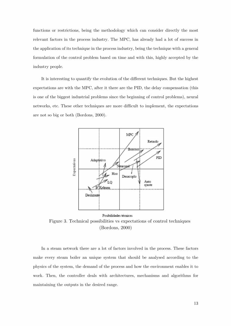
It is interesting to quantify the evolution of the different techniques. But the highest
expectations are with the MPC, after it there are the PID, the delay compensation (this
is one of the biggest industrial problems since the beginning of control problems), neural
networks, etc. These other techniques are more difficult to implement, the expectations
are not so big or both (Bordons, 2000).
Figure 3. Technical possibilities vs expectations of control techniques
(Bordons, 2000)
In a steam network there are a lot of factors involved in the process. These factors
make every steam boiler an unique system that should be analysed according to the
physics of the system, the demand of the process and how the environment enables it to
work. Then, the controller deals with architectures, mechanisms and algorithms for
maintaining the outputs in the desired range.
13

For these systems are described some characteristics as uncertainty, physical bounds,
safety bounds, etc. All these variables have to be included inside an optimization problem
in order to find the most convenient and general solution to the problem.
The implementation of adaptive structures and tractable online tuning procedures
should be integrated with robust MPC techniques to address some uncertainty explicitly
in the controller calculation and assure feasibility, economic efficiency and safety of
complex multi-variable systems (Grosso, 2012).
MPC is one of the most accepted methods to work with when the system is
multivariable with online control and very flexible in the treatment of uncertainties on
integrated forecasts, safety and monitoring.
2.3.2 General Considerations
MPC stands for a family of methods that select control actions based on optimisation
problems. It is one of the most successful control approaches that has been applied to a
wide variety of application areas due to its capability to explicitly incorporate constraints
and define multiple performance objectives within a single control problem (Camacho &
Bordons, 2004).
The tractability of an MPC problem, especially when dealing with large-scale systems, is
defined by the nature of the elements that are involved in the predictive and optimisation
strategy. The use of a cost function allows to describe the desired behaviour of the system
and is generally defined under two purposes: stability and performance. It serves also to
specify preferences in a multi-objective optimal control problem (Camacho & Bordons,
2004). This element is application-dependant but there exist within the MPC literature
common cost functions which are convex and results in an easy to solve problem.
Common choices are based on linear (i.e.,|| ||1 , and || ||∞) and quadratic norm costs (i.e.,
|| ||2), which are usually weighted. The explicit handling of constraints is the key strength
of MPC (Maciejowski, 2002). In different applications the following types of constraints
can be found: linear (used to upper/lower bound variables), convex quadratic (used to
bound a variable to lie within an ellipsoid), probabilistic (used to deal with uncertainty
14

and to reduce conservatism of worst-case approaches), second order cones, switched
constraints (used when the inclusion of the constraint depends on meeting a predefined
condition), non-linear constraints (compromises any other type of constraint and are very
difficult to handle when solving the optimisation problem). The most critical element in
the MPC framework is the dynamic model of the system, since the robustness and
performance of the controller depends on the model which can be deterministic or
stochastic, linear or nonlinear, continuous or discrete or hybrid (Rossiter, 2003).
Figure 4. The model structure used in the MPC controller (Mathworks, 2016)
A general model used in MPC is given in the figure 4 that can include noise, disturbances,
measured and unmeasured inputs, measured and unmeasured outputs. Then, the steps
of resolution of the controller is to define the dynamics of the model and its constraints
subject to a cost function, which will depend on the horizon of prediction.
15

16

Chapter 3
3 Modelling a Steam Boiler
This chapter presents the modelling principles of the steam boiler. A case study with
data taken from a real plant will be analysed. This plant has been proposed as a
benchmark problem to be solved in a national and international competition. The
modelling strategy is based on a black box analysis, starting from the point that every
steam boiler system is different depending on the physics, environment, and distribution
network, among others. This means that a rigid physical description of the model will
not work in the expected way for every steam boiler, thus deserving a distinguished
treatment.
3.1 General Description of the Case Study
The boiler model is carried out on the basis of physical laws, previous efforts in boiler
modelling, known physical constants, plant data, and heuristic adjustments. The
resulting fairly accurate model is nonlinear, fourth order, and include inverse response,
time delays, measurement noise models, and a load of disturbance component.
(Pellegrinetti & Bentsman, 1996)
3.1.1 Analysed Boiler Models
The model is able to be used for model-based online controllers. With this kind of
control system, the efficiency of the boiler is going to improve being nowadays very
important in terms of energy savings. Pellegrinetti and Bentsman (1986) noted that the
17

methods to obtain the correct model of any steam boiler plant are not readily found in
an open literature and are often specific to a particular system. The model try to specify
all the variables with its disturbances in a mathematical manner to be used in simulators
of steam generator systems.
The boiler model in which is going to be based this chapter contains nonlinearities,
noise as the normal plant, time delays and disturbances that are going to be managed in
the next chapters. The behaviour of the model represents the significant dynamics of the
boiler at Abbott Power Plant in Champaign, IL in the United States, in the normal
regimes as in the feasible abnormal ones. This model represents a complete boiler that
predicts process response in terms of the measured outputs like drum pressure, drum
water level and oxygen excess, to controllable input as air and fuel rates, steam demand
rate and flowrate of water, and also the disturbances and noises. The model uncertainties
are important too, because there are described values as the fuel calorific value in
combustion, the heat transfer coefficient variations inside the boiler which varies along
the time, distributed dynamics of steam generations, among others. (Pellegrinetti &
Bentsman, 1996)
Figure 5. Industrial Steam Generator Plant.
18

The simulator used in the benchmark competition that is going to be used is
encrypted, forcing to analyse the inputs and outputs of the model as a black box being
necessary to apply to system identification techniques. However, it is known that all the
steam boiler models are based on physical and thermodynamic laws, mass and energy
balances, heuristic knowledge of boilers behaviour and deterministic data.
Based on the Pellegrinetti and Bentsman specifications, the first group of equation
relates the control input valve position (u1,u2,u3) to the input flow rates for the fuel, air
and feed water flow rates respectively:
1qf QFCFu= (3.1) qf: fuel flow rate QFCF: Max fuel flow rate of the system
1u : valve position from 0 to 1
2qa QACAu= (3.2) qa: air flow rate QACA: Max air flow rate of the system
2u : valve position from 0 to 1
3qfw QCFWu= (3.3) qfw: water flow rate QCFW: Max water flow rate of the system
3u : valve position from 0 to 1
The differential equation for the drum pressure depends on the variable x4 which
corresponds to a exogenous variable, the fuel flow rate (u1), and the water flow rate (u3)
and is given as
9/81 4 1 1 3
9/81 4 1 1 3
1 2 3 40.00558 0.0280 0.01348 0.02493
x CP x x CP u CP u CPx x x u u= − + − +
= − + − +
(3.4)
CP1, CP2, CP3, CP4: Fitting variables 1x : Drum pressure differential equation
1x : Pressure of the steam
19

The oxygen level equation assumes complete combustion and in steady state can be
represented as
2100( )( ) 2
qa qfFAROqa qf AIRO
−=
+ (3.5)
2O : Oxygen excess FAR: relation of air needed to consume all the fuel AIRO2: percentage of oxygen in the air
where FAR is the air to fuel mass ratio for complete combustion (stoichiometric
relation), and AIRO2 is the mass ratio of air to oxygen in atmospheric air (generally near
the 0,2). Assuming a first order lag with time constant TAIR, the state equation of the
oxygen can be expressed as
[ ]
[ ]
2 2 2
2 2 2
1
16.492
x O xTAIR
x O x
= −
= −
(3.6) 2x : oxygen excess rate 2x : permitted oxygen excess
But due to the nonlinear behaviour, a linear equation could not describe very well
how the system evolves being necessary to create a new nonlinear relation to define better
the behaviour of the constant FAR described as follows
2
2
1 20.310629 16.2983
FAR FA O FAFAR O
= += + (3.7)
FA1, FA2: fitting variables for the relation fuel-air
In some models as in this case, the steam demand is already defined and it will be
treated as a measured disturbance input. However, the computation of this variable
involves an equation that depends on exogenous variables and the drum pressure
4 1
4 1
( 1 2)( 0.855663 0.18128)
qs x CQS CQS xqs x x
= −= −
(3.8)
20

qs: desired steam flow rate CQS1, CQS2: fitting variables of steam flow rate
The load level was computed from the steam flow rate and pressure. Then, the steady
state and the states varying on time are the following
4 111 12x CD u CD= + (3.9)
4 4 11( 11 12)
1x x CD u CD
TD= − − −
(3.10) CD1, CD2: fitting variables TD1: time constant for the steam rate
4x : variable produced from the steam flow and pressure data 4x : rate related with the steam flow
There are other complementary equations that help to define the rest of the states,
for example the density of the steam with a constant temperature will be only dependent
of the pressure inside the boiler and the density of the liquid has very low variations
11 2rhs CS x CS= + (3.11)
rhs: density inside the drum
CS1, CS2: fitting variables
The volume of water inside the drum depends on this density, the evaporation flow
rate (msd), the volume of water in the drum (vwd), the steam quality (a1) and the energy
given (ef)
11 1237633 174
ef CU qf CUef qf
= += + (3.12)
ef: normal evaporation flow
CU11, CU12: fitting variables for evaporation flow
31
1
1
VWxa
VWrhs
−=
− (3.13)
21

1a : relation for evaporation of water
VW: Volume of water
1KBef Rqfw qsKmsd
K− +
=+
(3.14)
K: quality of steam
R: constant for quality of the stream
3 11 0.159vwd VWVTx CVWD a msd= + + (3.15)
VT: Total volume of the drum
vwd: volume of water in the drum
The variables not defined correspond to constants of the system as volume of the
drum (VW, VT), the quality of the steam (K), etc. Some of these constants have physical
description and other becomes from linear or nonlinear fitting. And finally, the 3rd state
represents the density of the fluid (liquid and steam).
33
QCFWu qsxVT
−=
(3.16)
3x : fluid density
The outputs provide the proper scaling to match the Abbot boiler to the particular
boiler. So, it is needed to do several conversions of units to adapt it to the international
system
1 1y SCPx= , pressure in PSI (3.17)
2 2y x= , oxygen level in % (3.18)
3 1( 2)y SCWCXW vwd CXW= − , water level in inches (3.19)
4y qs= , the steam flow rate (3.20)
It is well known that when a model is more complex, it is supposed to be more
faithful to the essentials of the plant dynamics but in terms of control, the objective is
to use the simplest possible model but with the closest behaviour to the reality. So, there
22

is a balance that have to be taken into account at time of choose the correct method to
develop the control strategy.
In the Pellegrinetti and Bentsman model (Pellegrinetti & Bentsman, 1996), without
the modifications of the encrypted one, the description of the state-space nonlinear model
is as follows
1 11 4 1 12 1 1 13 3 3( ) ( ) ( ) ( ) ( )x t c x t x t c u t c u tτ τ= + − − − (3.21)
22 2 2 23 1 1 24 1 1 22 21 2
25 2 2 26 1 1
( ) ( ) ( ) ( )( ) ( )( ) ( )
c u t c u t c u t x tx t c x tc u t c u tτ τ τ
τ τ− − − − −
= +− − −
(3.22)
3 31 1 32 4 1 33 3 3( ) ( ) ( ) ( ) ( )x t c x t c x t x t c u t τ= − − + − (3.23)
4 41 4 42 1 1 43( ) ( ) ( )x t c x t c u t cτ= − + − + (3.24)
1 51 1 4( ) ( )y t c x t τ= − (3.25)
2 61 2 5( ) ( )y t c x t τ= − (3.26)
3 70 1 6 71 3 6 72 4 6 1 6
75 1 6 76 77 3 674 1 3 6 79
3 6 1 6 78
( ) ( ) ( ) ( ) ( )[ ( ) ][1 ( )]( )
( )[ ( ) ]
y t c x t c x t c x t x tc x t c c x tc u t c
x t x t c
τ τ τ ττ ττ ττ τ
= − + − + − −− + + −
+ − − + +− − +
(3.27)
4 81 4 7 82 1 7( ) [ ( ) ] ( )y t c x t c x tτ τ= − + − (3.28)
The equations show how the variable related with the steam demand (x4) take
influence over 3 states and 2 outputs and in 4 of them, this influence is nonlinear. So, it
is convenient to create a system around a point considering the constant steam demand.
The simplest model should be taken as the correct one in the same evaluations, a
linear controller can be taken to do some tests and compare the cost functions that were
assigned to these methods.
3.1.2 Known Conditions of the Model
All the units used in the model are in SI, all the English units where translated in
order to simplify the calculations. But, the input and outputs of the plant are presented
in a relative scale from 0 to 100. It is supposed that all the variables can be handled by
23

control valves and their actions are represented in the instrumentation field with numbers
from 0 to 1. Then, the scale used in the case of the transformed inputs and outputs
represents the opening percentage of the control valves.
The considered boiler used as case study works with dual fuel. In this case, the fuel
is going to be treated as a uniform substance with an unique calorific value but it can
increase the uncertainty in some stages. The fuel was measured for a constant steam
pressure (2.24 MPa) and ratio (22.100 kg/s) for one boiler in a group of them.
The variables to control are: Drum pressure, Level of the water in the drum and
Oxygen excess. These levels will be specified and need to be maintained despite the
variation mainly on the steam demand. There are other variations that affect less because
of the lower uncertainty but they are still important, as the fluctuation in the heating
values of the fuel and environment.
The desired steam pressured must be maintained at the outlet of the drum despite
the variations in the quantity of steam demanded. The water inside the tank is important
to be refrigerated when it comes overheated because the water will absorb the heat adding
some pressure which is easier to control in boilers. Finally, the mixture of fuel rate and
air rate inside the combustion chamber must meet standards of safety, efficiency, and
protection of the environment maintaining the correct percentage of excess of oxygen at
the output.
All the physical laws that characterize the boiler operation were developed for
decades. To this was added some of the following features to get. To obtain a better
adaptation to the Abbott boiler number 2: nonlinear combustion equation and a model
for excess of oxygen, including stoichiometric air-to-fuel ratio to combustion.
3.1.3 Encrypted Model
The considered boiler model can be seen as a MIMO with 3 inputs that can be
manipulated from 0% to 100% in order to modify the fuel rate, air rate and flowrate of
water. There also exists a limitation in the ratio of 1% per second, describing the common
24

restrictions of the industrial actuators. The model provides information about the three
mentioned outputs in a scale from 0% to 100% including noise in the sensors to simulate
the real plant. Then, there is a 4th input which is the steam demand that in this case is
a measurable disturbance. Finally, the boiler is encrypted and the use of tools for its
control is limited according the rules established in the control competition (Comité
Español de Automática, 2016).
Figure 6. MIMO block of the boiler and it internal structure (Comité Español de Automática, 2016)
The standard operational and initial conditions are:
Table 1. Initial conditions of the Steam Boiler
Variable Name % Type of Variable
Fuel Rate (2) 2u 40.59 Measured input
Air Rate (3) 3u 63.07 Measured input
Water Flowrate (4) 4u 35.06 Measured input
Drum Pressure (1) 1y 40.51 Measured output
Oxygen Excess (2) 2y 37.77 Measured output
Water Level (3) 3y 44.41 Measured output
Steam Demand (1) 1u 37.86 Measured disturbance
Additionally, several behaviours of plant are described that are taken as reference
and need to be followed by the controlled plant. The reference cases correspond to the
reference controller and the other with an experimental one. The changes in all the
25

variables are arbitrary selected but always the same, so the controller is adjusted
considering only these behaviours.
The variables changes their reference in some moment: the steam demand change it
during 50 mins s until 70 mins, and the reference is changed at the beginning of the
scenario for the other variables. All of these changes are applied to assess the model
validity and the performance of the controller to reach the correct reference with the
desired dynamics.
Figure 7. Steam demand pattern
Figure 8. Reference and measured outputs of the steam boiler case study
26

There are changes in the reference of the Drum Pressure when the system reach the
5 minutes (300 seconds) working, to check the performance of a normal controller to
react to the situation. However, for the second variable that corresponds to the Oxygen
Excess these changes affects a lot its behaviour, even if the change is caused by the steam
demand or by the required drum pressure. On other hand, the water level in the drum
seems hard to stabilize because involves some delays, but it is the less important in order
to control.
The outputs presented in Figure 8 were obtained when the inputs presented in Figure
9 are applied in both the reference (standard controller) and evaluation (advanced
controller) cases for a single operation point.
Figure 9. Input measured variables in the steam boiler case study
The inputs are very affected by the Steam Demand as it could be seen between the
50 and the 70 minutes (see Figures 9), and also for the drum pressure with different
stabilization times in all the variables. It is easy to see how the fuel and air flow are
27

much coupled, but the water flow variable needs more time to stabilize, even when the
reference controlled is evaluated. The control of water flow is less important than the
others, so it can be reflected on the weighting of the controller objectives.
3.2 Identification of the Plant
The identification of the plant starts defining the order of the model and the input
and outputs to model. The model has to describe the behaviour of the plant as accurate
as possible but also have to be simple to be useful for control design purposes. There
exists some references about how control oriented models were constructed for a classic
boiler and will be used to develop the new models for the considered boiler used as case
study.
There are some characteristics inside a plant that makes it unique and to identify
it is necessary a detailed analysis of the input/output data.
The boiler plant behaves as a MIMO system that presents a lot of internal
interaction, every input affects several outputs. For example, if the fuel increases, the
heat will increase, the temperature of the water increase, the mixture between water and
steam will tend to steam and with this, the pressure is going to increase too. But the
oxygen excess will go down as the water level inside the drum. Then, all the variables
were affected and this analysis can be developed for the other variables as can be seen in
the summary of results.
Figure 10 the type of models that can be identified using the MATLAB identification
toolbox that includes both static and dynamic models. Alternatively, models can be white
or black box. In the case of the white box type, a model is based on physical laws and
every detail is taken into account to have a good accuracy. Parameter estimation is
relatively easy if the model form is known but this is rarely the case. This is not the case
of an industrial steam boiler since it is not a simple system to describe and its behaviour
is non-linear. This is the reason why the black box approach will be applied, where it
does not matter how the model works inside but the dynamics is tried to adjust as much
28

as possible to the plant behaviour considering only the information of the inputs and
outputs.
Figure 10. Types of Models (Mathworks, 2016)
The majority of the numerical models assume a linear time-invariant (LTI) for the
system. Since the data is collected in a sampled manner, the model is represented as a
sampled continuous system .
A linear model is often sufficient to accurately describe the system dynamics around
a given operating point. If the linear model does not adequately reproduce the measured
output, a nonlinear model might be needed. Before building a nonlinear model, the best
is to try transforming the input and output variables such that the relationship between
the transformed variables is linear.
29

Black-box modelling is usually a trial-and-error process, where parameters are
estimated considering different structures and selecting the one that achieves best fitting
between real and estimated data. Typically, black-box approach starts with the simple
linear model structure and progress to more complex structures. It might also be chosen
a model structure because it is familiar with this structure or because specific application
needs.
Inside the black box methods, there are several linear models to choose available.
The various linear model structures provide different ways of parameterizing the transfer
functions G and H (being G the relation between the measured input and the measured
output and H the relationship between the disturbances at the output and the measured
output). When using input-output data to estimate a LTI model, you can configure the
structure of both G and H, according to Table 2.
Table 2. Parametrizations of the system components (Mathworks, 2016)
Model Type G and H functions
State Space Model Represents an identified state-space model structure,
governed by the equations: x Ax Bu Key Cx Du e= + += + +
where the transfer function between the measured input u and output y is 1( ) ( )G s C sI A B D−= − + and the noise transfer function is 1( ) ( )H s C sI A K I−= − +
Polynomial Model Represents a polynomial model such as ARX, ARMAX and BJ. An ARMAX model, for example, uses the input-output equation
( ) ( ) ( )Ay t Bu t Ce t= + , so that the measured transfer function G is 1( )G s A B−= , while the noise transfer function is 1( )H s A C−= The ARMAX model is a special configuration of the general polynomial model whose governing equation is: ( ) ( ) ( )Ay t BFu t CDe t= +
The autoregressive component, A, is common between the measured and noise components. The polynomials B and F constitute the measured component while the polynomials C and D constitute the noise component.
30

Transfer Function Model Represents an identified transfer function model, which has no dynamic elements to model noise behaviour. This object uses the trivial noise model H(s) = I.
Process Model Represents a process model, which provides options to represent the noise dynamics as either first- or second-
order ARMAX process (that is, ( )( )( )
C sH sA s
= , where C(s)
and A(s) are monic polynomials of equal degree). The measured component, G(s), is represented by a transfer function expressed in pole-zero form.
Taking into account this information, the way to proceed from this point is to select
the type of model and adjust it in discrete-time. Then, according to Pellegrinetti and
Morilla (Pellegrinetti & Bentsman, 1996) (Comité Español de Automática, 2016), the
model have 4 states, 4 inputs and 3 outputs. . However, structure selection process is
another way to discover the model structure that fits better the model and the data.
Figure 11. Conditions for the identification of State Space models
The model will be identified in state space because is the most suitable representation
for the MPC implementation.
Data is acquired with a sampling time of 3 seconds. The model structure
configuration is going to be set to all of the models by default based on a 4th order system
31

and the estimation options will be focused on prediction. The steam demand is
considered as a measured disturbance. In the considered identification scenario, the
demand is going to change, when the system reach the 50 minutes, the demand will
increase a 10% and then will decrease again to the original value. The results are
described in Figure 12.
Figure 12. Identified outputs of the plant using state space method and infinite horizon
In the simulated output (infinite horizon), the identification is not well adjusted to
the outputs of the system. This result gives a clue about how is the system behaviour,
while a linear system cannot describe the dynamics of the system in an acceptable way
when some steam demand vary. The fit of this system with simulated output is -200 %
average, so is necessary to apply significate changes on the treatment of this data and
improve the identified model through the use of the closed loop feedback. When the
horizon is shorter, the results are better until reach the 78% of model fit average. For
32

the second variable (Oxygen Excess) the fit is still inaccurate enough to consider it
acceptable, even when it describes well the dynamic of the system with horizon of 1.
Figure 13. Identified outputs of the plant by using the state-space method and one-step
ahead prediction horizon
Then, with the one-step ahead prediction, the model outputs followed the measured
ones. But there is still a big difference between the modelled and the real behaviour when
consider a linear model for the plant. So, this motivates the application of a nonlinear
identification to obtain a model that better describes the dynamics.
3.3 Variation of the measured disturbance
After obtain the model in a given operation point with not so good results on the
simulated output model, the next step is to apply some variations on the measured
33

disturbance (steam demand) taking care about the signals do not reach the maximum
and minimum values in any of the measured variables (inputs and outputs).
Figure 14. Variation of the Measured Disturbance (Steam Demand)
Figure 15. Outputs depending on the steam demand variation
This technique avoids the identification of additional nonlinearities on the system,
maintaining the essence of the plant and the normal behaviour. But also will define if
34

there is some kind of pattern every time the demand change its value, and figuring out
how this pattern can be represented by a multiple model that schedules with the value
of the measured disturbance.
There exist several approaches to multi-models that schedule with some measured
variable. On the most known is the Linear Parameter-Varying (LPV) approach, where
the system is not only characterized around a given operating point, but in a wide range
of operation points by modelling how the parameters vary with a measured variable
(scheduling variable). LPV systems are a very special class of nonlinear systems which
appears to be well suited for control of dynamical systems with parameter variations. In
general, LPV techniques provide a systematic design procedure for gain-scheduled
multivariable controllers. This methodology allows performance, robustness
and bandwidth limitations to be incorporated into a unified framework (Balas, 2002).
The other option is to apply a controller in each point and apply the Takagi-Sugeno
(or Fuzzy Multi-model) approach, taking the values given by the closest controllers in
the operation points. Takagi-Sugeno controllers consist of an input stage, a processing
stage, and an output stage. The input stage maps sensor or other inputs, to the
appropriate membership functions. The processing stage invokes each appropriate rule
and generates a result for each, then combines the results of the rules. And the output
stage converts the combined result back into a specific control output value.
The inputs, as shown in Figure 16, vary depending on the demand. Based on the
steam demand figure were the grey colour corresponds to the lowest value of this variable
and cyan corresponds to the highest value, there are some behaviours that are important
to highlight:
- The output references can be followed correctly for all of the constant demand
values that were considered.
- The line which corresponds to the highest value of demand (50.5%), get on the
top of the second input, experimenting a saturation during a representative
period of time. This corresponds to nonlinear and a not desired behaviour in the
35

plant, being more influent in the second output that takes more time to get the
reference.
With higher values of demand, the inputs are higher too. All of them increase when
the demand increases and in a progressive way. This kind of behaviour have sense because
to satisfy the demand is necessary to increase the water flow and the heat, involving the
rising of the fuel and air flow.
Figure 16. Inputs depending on the steam demand variation
These results give a group of possible data to test and to generate the possible
models to work on. The same process is going to be taken into account to produce one
model for each steam demand value and check the results.
36

Figure 17. Outputs of the plant with a model identified in state-space, infinite prediction horizon and at steam demand at 37%
The results in Figure 17 show that simulated output (infinite horizon) follows very
well the real data. The model fit is over the 80% and follow the behaviour of the plant
in a correct way. The difference between the 80% and the 100% can be caused by the
noise, which is aleatory in both cases but the dynamics are very well described by all the
tested models.
The results are better when the horizon is shorter, but with this procedure the results
are almost the same. The models experiment an improvement with the reduction of the
horizon with all the tested demands and the maximum difference is located in the second
output (excess of oxygen) because of its nonlinear dynamics.
37

Figure 18. Outputs of the plant using a state-space method, one step ahead horizon and demand 37%
38

Chapter 4
4 MPC of the Boiler System
This chapter is deals with the application of MPC to the boiler system considered
as a case study in this thesis using the model obtained in the last chapter. The idea is
not only to control the system in a single operating point, but in a wide range of operating
points. The first step is to select a particular operating point and implement the control
around it. Then, a set operating points will be considered and bank of MPC controllers
fused using the Takagi-Sugeno approach will be developed.
4.1 Model-Based Predictive Controller
MPC is a control strategy that is very suitable for processes that present highly
coupled multivariable dynamics. This control strategy uses a mathematical model of the
process in order to predict the future behaviour of the system, and based on this, the
future control signal can be predicted (Camacho & Bordons, 2004), (Bedate Boluda,
2015).
The MPC can be considered as a control strategy based on an explicit use of the
internal mathematical model of the process to be controlled (prediction model). The
model is used to predict the evolution of the variables to control along of a temporary
prediction horizon. In the MPC strategy, the decision variables are calculated with an
online optimization process. The control criteria (or cost function) is related with the
39
future behaviour of the system, which is produced under a dynamic model named
prediction model.
The time horizon considered in the MPC optimization problem is defined by the
prediction horizon. The future behaviour of the system depends on the control actions
applied along the prediction horizon that are the decision variables.
The difference between the predictive behaviour and the real one is compensated
with the use of the feedback. This feedback is introduced by means of receding horizon
principle, which consists on applying only the first value of the sequence of control
actions, then the output system is measured to estimate the true system state and then
optimization is again solved with updated initial conditions (Mayne, Rawlings, Rao, &
Scokaert, 2000).
One of the most attractive properties of the MPC strategy is the flexibility of
problem formulation, where the system can be linear or not, MIMO, SISO with any
combinations, and the consideration of the constraints to the system, even if they are
soft, hard, physical or a signal limitations.
Any MPC imply the solution of an optimization problem in open loop and the
application of the receding horizon philosophy. The MPC optimization is based on the
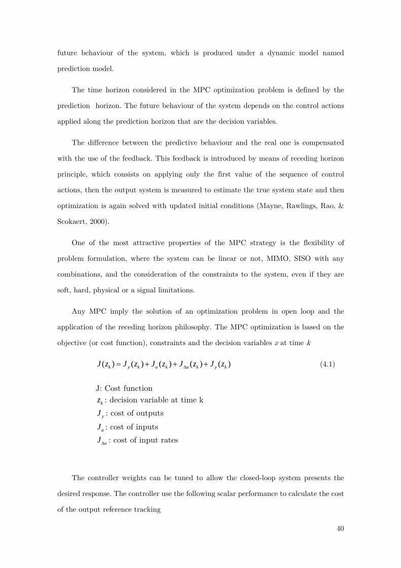
objective (or cost function), constraints and the decision variables z at time k
( ) ( ) ( ) ( ) ( )k y k u k u k y kJ z J z J z J z J z∆= + + + (4.1)
J: Cost function kz : decision variable at time k
yJ : cost of outputs
uJ : cost of inputs
uJ∆ : cost of input rates
The controller weights can be tuned to allow the closed-loop system presents the
desired response. The controller use the following scalar performance to calculate the cost
of the output reference tracking
40

2
,
1 1 ,
( ) ( | ) ( | )y yn p
i jy k j jy
j i i j
J z r k i k y k i ksω
= =
= + − +
∑∑ (4.2)
For the manipulated variable tracking and rate are the following
21
,, arg
0 0 ,
( ) ( | ) ( | )y un p
i ju k j j t etu
j i i j
J z u k i k u k i ksω−
= =
= + − +
∑∑ (4.3)
21
,
0 0 ,
( ) ( | ) ( 1 | )y un p
i ju k j ju
j i i j
J z u k i k u k i ksω∆−
∆ ∆= =
= + − + −
∑∑ (4.4)
The constraint violation cost is defined as
2( )kJ z kρ= (4.5)
2kρ : penalization variables
The constraints are already described implicitly but they can be configured
depending on the needs of the user. In this case, it could be necessary to adjust them
including the inputs and their rate and outputs. With i=1:p and j=1:n
,min ,max,min ,max
( ) ( | ) ( )( ) ( )j j jy y
k j k jy y yj j j
y i y k i k y ie V i e V i
s s s+
− ≤ ≤ + (4.6)
,min ,max,min ,max
( ) ( 1| ) ( 1)( ) ( 1)j j ju u
k j k ju u uj j j
u i u k i k u ie V i e V i
s s s+ − −
− ≤ ≤ + − (4.7)
,min ,max,min ,max
( ) ( 1| ) ( 1)( ) ( 1)j j ju u
k j k ju u uj j j
u i u k i k u ie V i e V i
s s s∆ ∆
∆ ∆ ∆
∆ ∆ + − ∆ −− ≤ ≤ + − (4.8)
ke : permitted error at time k
After defining the constraints and weights, the optimization problem associated to
the MPC can be formulated in way that can be solved using quadratic programming
algorithm. By introducing the following change of variable
[ ], , , , ,0 0 0
d u v du v d d
d
x A B C B B B Dx A B B B C C D C
x A B
← ← ← ← ← ←
41

The desired states and values are defined with the sub index d.
Then, the prediction model is
( 1) ( ) ( ) ( ) ( )( ) ( ) ( ) ( )
u v d d
v d d
x k Ax k B u k B v k B n ky k Cx k D v k D n k
+ = + + += + +
(4.9)
Next, consider the problem of predicting the future trajectories of the model at time
k=0.
1 11
0 0( | 0) (0) ( 1) ( ) ( ) ( )
i ii i
u v vh h
y i C A x A B u u j B v h D v i− −
−
= =
= + − + ∆ + +
∑ ∑ (4.10)
Considering the prediction in the prediction horizon p
1
(1) (0) (0)(0) ( 1)
( ) ( 1) ( )x u u v
y u vS x S u S H
y p u p v p
∆ = + − + + ∆ −
(4.11)
where
2
11
0
1 2
0 0
1 2
,
000
0
y x y x
y x
u
u upn n pn n
x up
p hu
h
u
u u upn n
up p
h huu u
h h
v v
v u vv
p pv v
CBCA
CB CABCA
S S
CA CA B
CBCB CAB CB
S
CBCA B CA B
CB DCAB CB D
H
CA B CA B CA
× ×
−
=
×
− −
= =
− −
+ = ∈ℜ = ∈ℜ + = ∈ℜ
=
∑
∑ ∑
3
00
y xpn n
pv vB D
×
−
∈ℜ
(4.12)
The MPC optimization problem can be converted to the general form of a QP
problem
42

12
oe oe
xMin x Hx f x +
, subject to Ax b≥ (4.13)
that can be efficiently solved with numerical solvers available nowadays.
4.1.1 Nonlinear MPC considerations
All the industrial processes are nonlinear, just as the one presented in this thesis.
However, the most of the control techniques are based on linear models, because of the
simplicity of identification and control of such models. Besides, linear models are very
close to the reality when the operation point is around the point where the system is
working (Bedate Boluda, 2015). Moreover, the use of linear models leads to convex
optimization problems that can be solved efficiently using numerical optimization
algorithms guaranteeing the global optimum. Thus, the model should not have strong
nonlinearities in order to have trustful results.
If nonlinear behaviour is important, then a linear controller cannot guarantee the
stabilization and performance of the closed-loop. Then, a nonlinear strategy should be
used. But in non-linear predictive control, the optimization process is nonconvex, which
is more complex that convex optimization problems. Thus, the computational time is
also longer. And, moreover, the achievement of the global optimum can not be
guaranteed.
Finally, the controller design becomes very complex in terms of stability, robustness,
perturbations, etc.
4.1.2 MPC Toolbox
MPC Toolbox provides functions, an GUI-based design application, and Simulink
blocks for systematically analysing, designing, and simulating MPC controllers. The
disturbances models can be specified, as well as MPC parameters: horizons, constraints,
and weights. The toolbox enables to diagnose issues that could lead to run-time failures
and provides advice on tuning weights to improve performance and robustness. By
43

running different scenarios in linear and nonlinear simulations, the controller
performances can be evaluated (Mathworks, 2016).
The performance of the controller can be evaluated while it runs by tuning weights
and varying constraints. Model predictive controllers can be used to optimize closed-loop
system performance of MIMO plants subject to input and output constraints. Because
they base their actions on an internal plant model, model predictive controllers can
forecast future process behaviour and compute the optimal control actions accordingly.
The ability to model process interactions often enables model predictive controllers to
outperform multiple PID control loops, which require individual tuning and other
techniques to reduce loop coupling.
Once defined the internal plant model, the design of the model predictive controller
can be completed by specifying the following controller parameters:
- Control interval (sample time)
- Prediction and control horizons
- Scale factors for plant inputs and outputs
- Hard and soft constraints on manipulated variables, manipulated variable rates,
and output variables
- Weights on manipulated variables, manipulated variable rates, and output
variables
- Models that characterize measurement noise and unmeasured input and output
disturbances
On rare occasions when the optimization may fail to converge due to process
abnormalities, the MPC Controller block freezes the controller output at the previous
value and lets you monitor optimization status at run time.
The MPC controller block also let access the optimal cost and control sequence at
each computation step. The signals can be used to analyse controller performance and
develop custom control strategies. However, this only applicable to an unique operation
44

point does not apply for all the evaluation range. In this case, other strategies should be
used as e.g., some gain-scheduling approach.
Figure 19. Comparison of workflows of the system and the Model Predictive Controller Toolbox
The workflow of the Figure 19 shows that the traditional design describe very well
the system that needs to be controlled. The next step is based on define the type, units
and nominal values of the plant inputs in order to control the system.
The input properties are very similar, the encrypted plant manipulates the variables
in a percentage way, being 0 the lowest value and 100 the highest (see Table 3). Thus,
the nominal value is the difference between both and is the same for all of them. The
measured disturbance is considered as an input to the MPC and to the plant.
45

Table 3. Input signal properties
Name Type Description Units Nominal
U1 Measured Disturbance Steam Demand % 100
U2 Manipulated Fuel Flow % 100
U3 Manipulated Air Flow % 100
U4 Manipulated Water Flow % 100
Table 4. Output signal properties
Name Type Description Units Nominal
Y1 Measured Output Drum Pressure % 100
Y2 Measured Output Oxygen Excess % 100
Y3 Measured Output Water Level % 100
The output properties follow the same line than the input properties (see Table 4).
The next step is to simulate the plant and see the behaviour that it takes at short and
long term.
4.1.3 Constraints
MPC allows implementing constraints in an easy way, even if they are inside the
process in a physical way or if they are controlled for better performance in a virtual
way. This kind of signals is processed and the constraints will limit the dynamic of the
system at all times. Several type of constraints can be considered: soft, hard and rate
constraint for every type of signal being inputs and outputs the usual ones.
By default, when the controller object is created, no constraints exist. To include a
constraint, the appropriate controller property should be set. Table 5 summarizes the
controller properties used to define most MPC Toolbox constraints. (MV = plant
manipulated variable; OV = plant output variable; MV increment = uk – uk-1).
46

Table 5. Constraint characteristics by default (Mathworks, 2016)
To include this constraint Set this controller property
Soften constraint by setting
Lower bound on MV MV(i).Min > -Inf MV(i).MinECR > 0 Upper bound on MV MV(i).Max < Inf MV(i).MaxECR > 0 Lower bound on OV OV(i).Min > -Inf OV(i).MinECR > 0 Upper bound on OV OV(i).Max < Inf OV(i).MaxECR > 0
Lower bound on MV increment MV(i).RateMin > -Inf MV(i).RateMinECR > 0 Upper bound on MV increment MV(i).RateMax < Inf MV(i).RateMaxECR > 0
From this table, it can be seen how the first applied controller is unconstrained but
it can be changed according to the parameters of the given system. There are some
considerations to take into account for the different manipulated and output variables,
where the rate constraints are more important in the MV and almost unnecessary for the
OV, even the OV constraints should be soft and in the MV not.
Hard constraints are constraints that the MPC must satisfy. If it is mathematically
impossible to satisfy a hard constraint at a given time instant, k, the MPC optimization
problem is infeasible. If the condition leading to infeasibility is not solved, infeasibility
can continue indefinitely, leading to a loss of control.
Disturbances and prediction errors are inevitable in practice. Therefore, a constraint
violation could occur in the plant even though the controller predicts otherwise. A feasible
optimization solution does not guarantee that all hard constraints will be satisfied when
the optimal MV is used in the plant.
When there are hard constraints on plant outputs, or hard custom constraints (on
linear combinations of plant inputs and outputs, and the plant is subject to disturbances,
the MPC optimization could be infeasible (Mathworks, 2016).
When a constraint is soft, the controller can deem an MV optimal even though it
predicts a violation of that constraint. If all plant outputs, MV increment, and custom
constraints are soft (as they are by default), the MPC optimization infeasibility does not
occur. However, controller performance can be suboptimal.
47

Table 6. Constraints configuration of the model
Name Units Minimum Maximum MaxDown Rate MaxUp Rate
Y1 % 0 100 - -
Y2 % 0 100 - -
Y3 % 0 100 - -
U2 % 0 100 -3 3
U3 % 0 100 -3 3
U4 % 0 100 -3 3
The constraints define the maximums and minimums values of the plant, in rate and
in nominal values. In the considered boiler plant, there are some constraints that are soft
but almost all of them are defined as hard, because the limits are defined from 0 to 100
percent supposing the minimum and maximum value that any variable can take and
nothing can go below or over these values. The other constraints are the rate, defined as
hard as well because the requirements of the plant specify that the maximum rate of any
variable that the system can provide to every input is 3% or -3%. This kind of limitations
are physical limitations and not because of performance, so the softening of them can not
be applied.
The unconstrained models gives non desired responses, the inputs and outputs go
beyond the physical barriers, just as in the case of controllers like the PID. This is one
of the greatest advantages of the MPC, as seen in the lasts figures, the performance is
the best achievable inside the proposed limits.
In order to control a MIMO system, it is needed to evaluate which variables are
more important and tune the weights until find the best response or the lowest value
taken from the defined cost function.
The result of the evaluation with constraints are presented n the Figure 20 and
Figure 21, where can be seen the respective inputs and outputs of the simulated system
as an internal model.
48

Figure 20. Inputs of the model with constraints
Figure 21. Outputs of the model with constraints
49

4.1.4 Weights
The weights are very important in order to set priorities to every input based on the
needs of every output at each sampling time. The toolbox lets adjust individual
weights on manipulated variables, manipulated variable rates, and output variables.
MPC designer GUI-application also provides additional weight-tuning capability to make
the controller more robust or more aggressive. A controller is provided to tuning aid to
compute effect of weights on performance and to suggest weight adjustments to improve
controller design.
The toolbox let adjust the weights of a model predictive controller to optimize its
performance at run time without redesigning or reimplementing it. The weights that can
be tuned are the following:
- Weights on plant outputs - Weights on manipulated variables - Weights on manipulated variable rates - Weight on overall constraint softening
The toolbox provides a diagnostic function for detecting potential stability and
robustness issues with your model predictive controller, such as:
- Model predictive controller or closed-loop system is unstable - QP optimization problem is ill-defined with an invalid Hessian matrix - Zero steady-state offset cannot be achieved - Hard and soft constraint settings may lead to infeasible optimization problems
at run time
A diagnostic tool can be used to adjust controller weights and constraints during
controller design to avoid run-time failures. The diagnosis starts with the definition of
the set-points and then adjusting all the weights considering which variables all more
important than others. In the boiler case study, the level inside the boiler is much less
important than the other two variables in terms of control, but maintain the pressure
inside the boiler is necessary to send the exact demand out of the system and maintain
the temperature regulations. The oxygen excess is more related to safety reasons and is
the second important output to control.
50

Table 7. Set point values of the plant
Name Units Type Initial Size Time Period
Y1 % Step 41 -5 300 -
Y2 % Step 38 -5 600 -
Y3 % Constant 44 - - -
U1 % Pulse 40 5 3000 1200
Table 8. Tuned Weights to control the model
Name Description Units Weight Rate Weight
U2 Fuel Flow % 0.3 0.1
U3 Air Flow % 0.3 0.1
U4 Water Flow % 0.3 0.1
Y1 Drum Pressure % 15 -
Y2 Oxygen Excess % 10 -
Y3 Water Level % 2 -
Figure 22. Model inputs after tuning the weights
51

The initial conditions are settled for all the input and output variables and to test
the MPC the values will be taken by default.
Figure 23. Model outputs after tuning the weights
4.2 Nonlinear Controller Approximations
An approach to take into account the nonlinearities of the plant in the control design
is now presented. According the modelling part of the thesis, the dynamics of the boiler
system presents a non-linear behaviour. In general, most of the heat transfer systems
are not well described by linear approximations, but when the reactions inside a chamber
are occurring, this kind of dynamics become more and more complex and are impossible
in some cases to be described by linear systems in only one operational point. That is the
reason why the chemical processes are the reference in terms not only of the Model
Predictive Control, if not the nonlinear dynamics in the systems too.
Once discovered the variable that carachterizes the nonlinearities on the system,
the control should be focalized on minimize the action of this nonlinear behaviour and
52

try to apply all the techniques that are known when possible. It is important to maintain
the stability on the system, and use linear techniques when possible.
4.2.1 Considered Techniques
One of the most used strategies is the LPV or adaptive control (Reina, 2016). Both
techniques are accepted and have been studied for a considered time being very trustful,
of course there are some limitations on both of them but they are still being a good option
at the moment of application.
Adaptive control is the control method used by a controller which must adapt to
a controlled system with parameters which vary, or are initially uncertain (Landau,
1979). This method adapts the controllers to both the process statics and dynamics. In
special cases, the adaptation can be limited to the static behaviour alone, leading to
adaptive control based on characteristic curves for the steady-states or to extremum
value control, optimizing the steady state. Hence, there are several ways to apply
adaptive control algorithms. But this technique has a particular inconvenience, for several
variables (more than 3) the problem becomes very complex and is not easy to follow how
the variables change with respect the variations of the inputs.
So, this is very much recommended when the parameters are very explicit and for
SISO systems or with one or two variables more. Onn the other hand, the LPV controllers
are often designed at various operating points using linearized models of the system
dynamics that are scheduled as a function of a parameter or parameters for operation at
intermediate conditions. It is an approach for the control of non-linear systems that uses
a family of linear controllers, each of which provides satisfactory control for a different
operating point of the system (Wu, 1995). One or more observable variables, called
the scheduling variables, are used to determine the current operating region of the system
and to enable the appropriate linear controller. In brief, gain scheduling is a control
design approach that constructs a nonlinear controller for a nonlinear plant by patching
together a collection of linear controllers. These linear controllers are blended in real-
time via switching or interpolation.
53

Scheduling multivariable controllers can be very tedious and time-consuming task.
4.2.2 Takagi-Sugeno
An approach similar to the LPV one has been developed in parallel and it is known
as Takagi-Sugeno (TS) Fuzzy Systems. A fuzzy controller uses fuzzy rules, which are
linguistic if-then statements involving fuzzy sets, fuzzy logic, and fuzzy inference. Fuzzy
rules play a key role in representing expert control knowledge and experience and in
linking the input variables of fuzzy controllers to output variable (or variables).
The fuzzy model has to satisfy the same requirements of the MPC models and its
implementation. The Takagi-Sugeno model can be obtained based on physical or input-
output data and then implement the controller based on the model. So, it can be seen
how is totally compatible with the development of the MPC method.
The MPC features are a prediction model, a decision criteria, and optimizer and a
mobile horizon. For the fuzzy control, there are some techniques to apply fuzzy models
in order to get the prediction in the established horizon and this prediction is generally
based on linear models (Souda, Babuska, Brujin, & Verbruggen, 1996).
Fuzzy control is based on fuzzy rules. In this thesis, MPC is used to control the
boiler case study including constraints and cost functions, that here will be combined
with fuzzy Takagi-Sugeno approach.
On practical applications of MPC to nonlinear systems, it is difficult to find a trustful
model for prediction. However, fuzzy Takagi-Sugeno techniques can provide a good and
linear-like representation of nonlinear systems, being possible to develop extensions of
current control approaches for linear systems.
The fuzzy models are considered as a battery of linear models or almost linear
(Huang, Lou, Gong, & Edgar, 2000). The main problem with the fuzzy models is that
they do not allow including constraints on the process variables as inputs, outputs and
rates, being necessary to resort to traditional predictive control techniques.
54

There are some new techniques that explain how to use the predictive control on
fuzzy Takagi-Sugeno models but there are also several solutions for this. In this case, the
idea is to implement the MPC controller with the internal model designed under this
method and then the fuzzy model is applied. After all this, there is a cost function that
involves the control objectives used for controlling the system.
Figure 24. Model Based Fuzzy control design (Tanaka & Wang, 2001)
The Takagi-Sugeno decision rules can be designed based on arbitrary rules, taking
into account how the controllers work. First, the range of correct action for each
controller around the operation point should be known. Then, note that if there is any
other controller near this point that can perform better, classify them and choose. In this
case, the controllers are similar between them. But, if there are more controllers, then
there are a lot of operating points covered.
In the boiler case study, the range of action of each controller can be 5%, so from
37.5% to 50% of steam demand, three controllers can be used to cover all the necessary
values of control action. However, to be more accurate, the number of controllers is raised
to five, which means that there will be more points where the controllers are well defined.
55

Figure 25. Takagi-Sugeno Decision rules
In the boiler case study, the range of action of each controller can be 5%, so from 37.5%
to 50% of steam demand, three controllers can be used to cover all the necessary values
of control action. However, to be more accurate, the number of controllers is raised to
five, which means that there will be more points where the controllers are well defined.
In general, the fuzzy model is based on decisions and are characterized by a set of
rules and discrete-time models
Discrete Fuzzy System (DFS)
Model Rule i:
IF 1( )z k is 1iM and and ( )pz k is ipM
THEN ( 1) ( ) ( ),
1, 2, ,( ) ( ),
i i
i
x k A x k B u ki r
y k C x k+ = +
= =
The next step is to define how the models are combined taking into account the
value of steam demand. In this case, z(k) is the steam demand, M is the number which
will go from 35% to 50% and the system is the discrete-time model identified for each
demand and there will be as much rules as controllers (5). The outputs of the fuzzy
system is inferred as follows
SS1 SS2 SS3 SS4 SS5
56

( ){ }
( )
( ){ }
1
1
1
( ) ( ) ( )( 1)
( )
( ) ( ) ( ) ,
r
i i ii
r
ii
r
i i ii
w z k A x k B u kx k
w z k
h z k A x k B u k
=
=
=
++ =
= +
∑
∑
∑
(4.14)
( )
( )
( )
1
1
1
( ) ( )( )
( )
( ) ( ),
r
i ii
r
ii
r
i ii
w z t C x tx t
w z t
h z t C x t
=
=
=
=
=
∑
∑
∑
(4.15)
where
[ ]1 2 3
1
1
( ) ( ) ( ), , ( ) ,
( ( )) ( ( )),
( ( ))( ( ))( ( ))
p
i ij jj
ii r
ii
z t z k z k z k
w z t M z k
w z kh z tw z k
=
=
=
=
=
∏
∑
(4.16)
for all k. The term ( ( ))ij jM z k is the grade of membership of ( )jz k in ijM . Since
1( ( )) 0,
( ( )) 0,
r
ii
i
w z k
w z k=
> ≥
∑ i=1,2,…,r, (4.17)
1( ( )) 0,
( ( )) 0,
r
ii
i
h z k
h z k=
> ≥
∑ i=1,2,…,r, (4.18)
From Figure 25, the zones that correspond to each model and that will be also use
for each controller udinh the IF-THEN rules for the steam demand ( measured
disturbance)
57

Model Rule 1:
IF Demand is M1(37.5)
THEN 1 1
1 1
( 1) ( ) ( )( ) ( ) ( )
x k A x k B u ky k C x k D u k+ = +
= +
Model Rule 2:
IF Demand is M2(40.5)
THEN 2 2
2 2
( 1) ( ) ( )( ) ( ) ( )
x k A x k B u ky k C x k D u k+ = +
= +
Model Rule 3:
IF Demand is M3(43.5)
THEN 3 3
3 3
( 1) ( ) ( )( ) ( ) ( )
x k A x k B u ky k C x k D u k+ = +
= +
Model Rule 4:
IF Demand is M4(46.5)
THEN 4 4
4 4
( 1) ( ) ( )( ) ( ) ( )
x k A x k B u ky k C x k D u k+ = +
= +
Model Rule 5:
IF Demand is M5(49.5)
THEN 5 5
5 5
( 1) ( ) ( )( ) ( ) ( )
x k A x k B u ky k C x k D u k+ = +
= +
where
1
0,991 0,009 0,009 0,0320,014 0,944 0,023 0,021
0,009 0,008 0,924 0,2950,008 0,113 0,059 0,252
A
=
−−
−
−
−− −
, 2
0,994 0,000 0,012 0,0120,009 0,953 0,007 0,0690,005 0,020 0,986 0,1200,066 0,077 0,058 0,504
A
=
−−
−
−
−
3
0,988 0,004 0,023 0,1210,000 0,941 0,038 0,088
0,008 0,033 0,928 0,2500,034 0,024 0,258 0,573
A
−−
− −
=
− − −
, 1
0,988 0,007 0,030 0,0710,007 0,993 0,055 0,1630,008 0,006 1,044 0,2720,014 0,023 0,187 0,513
A
= −
− − −
−
58

1
0,986 0,015 0,009 0,1290,040 0,916 0,002 0,164
0,015 0,045 0,970 0,0430,049 0,106 0,128 0,682
A
= −
−
−
, 1
0,000 0,000 0,001 0,0020,005 0,001 0,002 0,002
0,014 0,004 0,011 0,0140,017 0,012 0,031 0,038
B
−− − −
− −−
=
−
2
0,000 0,000 0,000 0,0000,007 0,000 0,001 0,0010,007 0,000 0,002 0,0030,011 0,000 0,012 0,017
B
=
− −− −− −
, 3
0,008 0,000 0,001 0,0050,010 0,000 0,000 0,0020,020 0,001 0,003 0,008
0,105 0,007 0,022 0,062
B
− −−− −
− −
=
4
0,002 0,000 0,001 0,0010,005 0,001 0,002 0,0030,012 0,002 0,003 0,004
0,013 0,003 0,006 0,008
B
=
− −− −− −
− −
, 5
0,011 0,002 0,001 0,0050,017 0,002 0,001 0,0040,001 0,001 0,001 0,003
0,143 0,029 0,016 0,062
B
=
− −− −− −
− −
1
11,342 11,182 9,532 4,84772,790 14,607 1,798 4,7197,127 8,320 5,400 4,682
C =
− −
− , 1
5,700 9,908 10,216 1,73467,041 4,885 1,876 6,1942,684 9,360 3,242 5,400
C =
−−
− −
−−−
1
0,868 11,242 12,964 2,01066,534 0,701 2,697 6,1261,269 8,337 5,438 6,128
C = −
−−
−, 1
7, 231 17,939 4,739 5,38061,608 8,265 0,582 9,888
1,197 4,916 9,315 5,050C
=
− −−
− −
1
1,397 6,351 10,754 1,63957,604 10,119 2,876 5,940
6,259 12,238 0,979 6,827C
− − −− −
− − −
=
Another idea is to combine the nearest controllers according the steam demand. For
example, if the steam demand in the middle of both controllers, take the half of both and
sum them to have the interpolated value of control. The parallel distributed
compensation (PDC) offers a procedure to design a fuzzy controller from a given model.
To realize the PDC, the nonlinear system is first represented by a TS model and then
each control rule is designed from the corresponding rule of the model. The controller
needs to share the same premises than the MPC and to construct it the steps bellow
were followed;
59

Model Rule i:
IF 1( )z k is 1iM and and ( )pz k is ipM
THEN ( ) ( ) 1, 2, ,iMPCu k u k i r= =
The fuzzy control has a linear controller (battery of MPCs in this case) in
the consequent parts. The overall fuzzy controller is represented by
( )
( )( )
1
1
1
( ) ( )( ) ( ) ( ),
( )
i
i
j
i MPC ji j
i MPCji j
ii j
w z k u ku k h z k u k
w z k
+
+=
+=
=
= =∑
∑∑
where j is the nearest bottom
value of z(k).
Figure 26. Takagi-Sugeno with PDC based on two controllers
The limitation of this approach is the computational time since several MPC
controllers should be run in parallel.
4.3 Implementation on Plant
Once the proposed approach has been presented the details regarding the
implementation are given.
60

4.3.1 MPC Block
Figure 27 shows how the integrated controller to the boiler simulator, the MPC block
that contains the controller already designed is updated with the readings of the
measured variables and tuned by means of weights, constraints, ratios, etc.
Figure 27. MPC Block in the simulator
Figure 28. MPC outputs implemented on plant without tune
61

From Figure 28, it can be seen that the outputs do not reach the expected set-points.
Then, it is necessary to tune appropriately the MPC controller by modifying the tuning
parameters.
Figure 29. MPC inputs implemented on plant without tune
There are several issues to take into account in the tuning of the MPC in the correct
direction:
- The outputs do not follow the references as well as when simulated using the
MPC internal model. Then, the tuning is important in terms of weight for each
variable in order to reduce the cost of this run which is 114.14 units. The tuning
needs to be focalized in follow the references of the excess of oxygen, drum
pressure and finally the water level inside the drum.
- Since the controller output is quite noisy, the idea is to increase the weight of
the input rate until it behaves smoothly.
- Even when the demand is constant, there is an strange behaviour to take into
account and studied with series of simulation focalized in this dynamic. To
62

resume, the level of the water inside the drum increase all what it can get in
short time (2 mins approximate), and then decrease in 3 seconds until zero
percent again. During this interval, the pressure inside the drum increase too
and the excess of oxygen keeps oscillating.
- On the other hand, the inputs vary only in the air flow and in the fuel flow,
both variables do not give mass and then no pressure to the drum (see Figure
5). The only input variable that can give mass to the drum is the water flow
and this variable is zero percent during the 2 hours of simulation. Even with
this input signal being zero, the pressure and the steam demand keeps ‘constant’
and the level of water inside the drum increase during a representative period
of time (5 minutes). This is a very important result, even when the control was
not so good.
4.3.2 Tuning
Using a bank of MPC designed for each local model of the TS model presented in
previous section and fusing the controllers in the same way that local models, several
parameters had to be properly tuned to achieve the desired performance.
The safety parameters that produce an emergency stop on the plant are not taken into
account here. But, the designed control should satisfy the minimum requirements to
handle all the variables and guarantee safety in all aspects such that the risks will be
minimized. The MPC tuning parameters can be manipulated online. The first tuning
adaptation is based on how good the references are followed and then the proportion of
the noise against the magnitude of the signal are considered too. The weights are modified
from one simulation to other in order to get the expected results.
The first characteristic to note is that the inputs were limited, basically the water
input because in a system that handle a lot of energy converted in temperature is not
possible to have for a long time 0% of water flow into the system. The noise was corrected
with an important increment in the weight of the rate in the inputs and the weights of
the outputs were tuned too, but using very similar values. The references were changed
63

several times to demonstrate how the system follows the established set point. And,
finally the 3rd output was limited between the values around the desired point.
Figure 30. Input in the tuned MPC
The first characteristic to note is that the inputs were limited, basically the water
input because in a system that handle a lot of energy converted in temperature is not
possible to have for a long time 0% of water flow into the system. The noise was corrected
with an important increment in the weight of the rate in the inputs and the weights of
the outputs were tuned too, but using very similar values. The references were changed
several times to demonstrate how the system follows the established set point. And,
finally the 3rd output was limited between the values around the desired point.
64

Figure 31. Outputs of the tuned variables
Figure 32. Inputs obtained using the Takagi Sugeno’s technique
65

Figure 33. Outputs obtained using the Takagi-Sugeno’s technique
Figure 34. Steam produced using the -Sugeno’s technique
The inputs seems very normal in rate and limits, the water flow is in the lower limit
but keeps sending matter to the boiler to produce steam.
In the outputs, the behaviour is as expected with four changes on the steam demand.
The pressure in the boiler follows the reference during all the simulation and the oxygen
excess looks not so affected by the changes in the demand and in the drum pressure
references. Then the level of water inside the boiler is not relevant due to the null value
66

in the cost function of this variable, but is important to maintain it inside the limits.
The most penalized output was very well controlled allowing that the cost function
provides the lowest value for this sequence.
Finally, a cost function was tuned with the desired weights. For rate constraint, the
weight will be 20, the penalty for the drum pressure and for the oxygen excess will be
the same and tuned to 10. Finally, the level is limited and the importance of this variable
is not so representative. Thus, the value of the weight is 0.1. See (4.1), (4.2), (4.3) and
(4.4).
67


Chapter 5
5 Results
In this chapter, the results obtained with the applications of the identification and
control methods described in previous chapters are presented and analysed. First, the
results of the state space parameter identification are shown. Then, the models are
validated and the performance of the used controllers after the tuning are evaluated,
taking as reference the operational cost given by the system.
5.1 Boiler plant identification
For the identification of the plant, there were some characteristics of the system to
take into account. The procedure was the same to identify all the models for each of the
steam demand values considered. The obtained model is expressed in state space with 4
inputs and 3 outputs. The first is a measured disturbance (steam demand) and other
three are the controlled inputs correspond to fuel flow, air flow and water flow(See Table
1). On the other hand, the three outputs that correspond to the drum pressure, oxygen
excel and water level inside the drum. Thus, the matrix A is 4x4, B is 4x4, C is 3x4 and
D is 3x4 and the characteristics of the plant needs to be analysed to know how the
different inputs affect to each output.
The values of demand were taken from 35.5% until 50% where the dynamics of the
system operates inside the limits, avoiding other nonlinear behaviours as the saturation.
The values for each matrix when changing the demand are in Tables 9, 10 and 11.
69

Table 9. Difference of parameter in the matrix A of identification
Matrix# Colunm 1 Colunm 2 Colunm 3 Colunm 4 |Dif SSi.A| |Dif SSi.A| |Dif SSi.A| |Dif SSi.A|
ss1.A 35.5%
0,991 0,009 -0,009 0,032 0,003 0,016 0,023 0,030
0,014 0,944 0,023 -0,021 0,007 0,031 0,011 0,095 -0,009 0,008 0,924 -0,295 0,007 0,044 0,129 0,621
-0,008 -0,113 -0,059 0,252 0,000 0,005 0,056 0,302
ss2.A 37%
0,993 -0,007 0,013 0,002 0,001 0,007 0,002 0,014 0,007 0,976 0,012 0,074 0,002 0,022 0,019 0,143 -0,001 0,052 1,052 0,326 0,006 0,073 0,067 0,446
-0,007 -0,108 -0,115 0,554 0,073 0,185 0,172 0,051
ss3.A 38.5%
0,994 0,000 0,012 -0,012 0,008 0,018 0,020 0,136 0,009 0,953 -0,007 -0,069 0,008 0,009 0,013 0,088 0,005 -0,020 0,986 -0,120 0,020 0,016 0,035 0,207
0,066 0,077 0,058 0,504 0,075 0,026 0,114 0,531
ss4.A 40%
0,986 0,018 -0,008 -0,148 0,002 0,014 0,014 0,269 0,001 0,944 -0,020 0,019 0,001 0,003 0,019 0,069 -0,015 -0,005 0,951 -0,327 0,007 0,029 0,022 0,576
-0,009 0,103 -0,056 -0,027 0,024 0,127 0,314 0,546
ss5.A 41.5%
0,988 0,004 -0,023 0,121 0,000 0,011 0,030 0,031 0,000 0,941 -0,038 0,088 0,005 0,013 0,007 0,184 -0,008 -0,033 0,928 0,250 0,003 0,031 0,019 0,069
-0,034 -0,024 0,258 -0,573 0,042 0,080 0,277 0,570
ss6.A 43%
0,988 0,016 0,007 0,090 0,001 0,022 0,037 0,161 0,005 0,955 -0,031 -0,096 0,002 0,038 0,086 0,259 -0,010 -0,002 0,947 0,319 0,018 0,008 0,097 0,047
0,009 -0,104 -0,019 -0,003 0,005 0,081 0,168 0,516
ss7.A 44.5%
0,988 -0,007 -0,030 -0,071 0,000 0,013 0,023 0,164 0,007 0,993 0,055 0,163 0,025 0,070 0,073 0,310 0,008 0,006 1,044 0,272 0,008 0,061 0,089 0,321
0,014 -0,023 -0,187 0,513 0,035 0,123 0,340 1,042
ss8.A 46%
0,988 0,007 -0,007 0,092 0,002 0,008 0,016 0,222 0,032 0,923 -0,018 -0,147 0,008 0,007 0,020 0,311 0,016 -0,055 0,955 -0,049 0,032 0,100 0,014 0,092
-0,021 -0,146 0,153 -0,529 0,071 0,252 0,024 0,153
ss9.A 47.5%
0,986 0,015 0,009 -0,129 0,011 0,011 0,046 0,290 0,040 0,916 0,002 0,164 0,026 0,013 0,056 0,442 -0,015 0,045 0,970 0,043 0,026 0,033 0,086 0,410
0,049 0,106 0,128 -0,682 0,063 0,227 0,196 0,212
ss10.A 49%
0,976 0,026 -0,037 0,161 - - - - 0,066 0,904 0,058 -0,278 - - - - 0,011 0,013 0,884 0,453 - - - -
-0,013 -0,121 0,325 -0,470 - - - -
70

Table 10. Difference of parameter in the matrix B of identification
Matrix# Colunm 1 Colunm 2 Colunm 3 Colunm 4 |Dif SSi.B| |Dif SSi.B| |Dif SSi.B| |Dif SSi.B|
ss1.B 35.5%
0,000 0,000 -0,001 0,002 0,000 0,001 0,001 0,002
-0,005 -0,001 0,002 -0,002 0,001 0,001 0,003 0,003 0,014 -0,004 0,011 -0,014 0,017 0,006 0,017 0,019
0,017 -0,012 0,031 -0,038 0,017 0,008 0,021 0,030
ss2.B 37%
0,000 0,000 0,000 0,000 0,000 0,000 0,000 0,001 -0,004 0,000 -0,001 0,001 0,003 0,000 0,000 0,000 -0,003 0,002 -0,006 0,006 0,003 0,002 0,004 0,003
0,000 -0,003 0,010 -0,008 0,011 0,004 0,022 0,025
ss3.B 38.5%
0,000 0,000 0,000 0,000 0,006 0,002 0,004 0,006 -0,007 0,000 -0,001 0,001 0,003 0,001 0,002 0,003 -0,007 0,000 -0,002 0,003 0,012 0,004 0,007 0,010
-0,011 0,000 -0,012 0,017 0,036 0,015 0,019 0,029
ss4.B 40%
-0,007 0,002 -0,004 0,007 0,001 0,002 0,003 0,002 -0,004 -0,001 0,002 -0,002 0,006 0,001 0,002 0,004 -0,019 0,004 -0,009 0,013 0,001 0,003 0,006 0,005
-0,047 0,015 -0,032 0,046 0,152 0,022 0,054 0,107
ss5.B 41.5%
-0,008 0,000 -0,001 0,005 0,003 0,002 0,000 0,002 -0,010 0,000 0,000 0,002 0,013 0,003 0,003 0,006 -0,020 0,001 -0,003 0,008 0,006 0,006 0,003 0,001
0,105 -0,007 0,022 -0,062 0,040 0,017 0,000 0,027
ss6.B 43%
-0,005 0,002 -0,002 0,003 0,003 0,002 0,001 0,002 0,003 -0,003 0,003 -0,004 0,002 0,002 0,001 0,002 -0,025 0,007 -0,006 0,010 0,037 0,008 0,009 0,014
0,065 -0,024 0,022 -0,035 0,078 0,027 0,028 0,043
ss7.B 44.5%
-0,002 0,000 -0,001 0,001 0,006 0,001 0,000 0,002 0,005 -0,001 0,002 -0,003 0,011 0,001 0,001 0,001 0,012 -0,002 0,003 -0,004 0,004 0,001 0,003 0,004
-0,013 0,003 -0,006 0,008 0,143 0,029 0,022 0,070
ss8.B 46%
-0,008 0,002 -0,001 0,004 0,003 0,001 0,000 0,001 0,016 -0,002 0,001 -0,004 0,001 0,000 0,000 0,000 0,008 0,000 0,000 0,000 0,007 0,001 0,001 0,003
0,130 -0,026 0,015 -0,062 0,273 0,055 0,032 0,124
ss9.B 47.5%
-0,011 0,002 -0,001 0,005 0,001 0,001 0,001 0,000 0,017 -0,002 0,001 -0,004 0,007 0,003 0,002 0,003 0,001 -0,001 0,001 -0,003 0,033 0,013 0,006 0,018
-0,143 0,029 -0,016 0,062 0,252 0,064 0,034 0,109
ss10.B 49%
-0,012 0,004 -0,002 0,005 - - - - 0,023 -0,006 0,003 -0,008 - - - - -0,032 0,011 -0,005 0,015 - - - -
0,108 -0,035 0,017 -0,047 - - - -
71

Table 11. Difference of parameter in the matrix C of identification
Matrix# Colunm 1 Colunm 2 Colunm 3 Colunm 4 |Dif SSi.C| |Dif SSi.C| |Dif SSi.C| |Dif SSi.C|
ss1.C 35.5%
11,342 -11,182 -9,532 4,847 3,709 0,133 19,131 0,748 72,790 14,607 1,798 4,719 0,419 11,004 6,289 2,526
7,127 -8,320 5,400 4,682 4,791 1,121 10,297 0,374
ss2.C 37%
7,633 -11,315 9,599 5,594 1,933 1,407 0,617 7,328 72,371 3,603 -4,491 7,245 5,330 1,282 2,615 13,439
2,336 -9,441 -4,897 4,308 0,349 0,081 1,656 9,708
ss3.C 38.5%
5,700 -9,908 10,216 -1,734 3,482 0,146 0,216 2,267 67,041 4,885 -1,876 -6,194 2,084 2,228 0,570 4,329
2,684 -9,360 -3,242 -5,400 0,730 0,498 1,043 0,237
ss4.C 40%
2,218 -9,762 10,000 -4,001 1,349 1,480 2,964 6,010 64,957 2,657 -1,305 -10,523 1,577 1,956 1,392 16,649
1,955 -8,861 -4,285 -5,163 0,685 0,525 1,153 11,291
ss5.C 41.5%
0,868 -11,242 12,964 2,010 1,545 4,884 4,130 3,576 66,534 0,701 -2,697 6,126 13,366 4,128 1,833 1,848
1,269 -8,337 -5,438 6,128 0,701 3,417 2,777 0,633
ss6.C 43%
2,414 -16,126 8,834 5,585 4,817 1,813 4,095 10,966 53,168 4,829 -0,864 7,974 8,441 3,436 1,446 17,862
1,971 -4,920 -8,215 5,495 3,167 9,836 17,530 10,544
ss7.C 44.5%
7,231 -17,939 4,739 -5,380 1,895 8,181 6,403 6,879 61,608 8,265 0,582 -9,888 0,539 1,422 1,865 14,922
-1,197 4,916 9,315 -5,050 3,441 5,993 5,555 11,746
ss8.C 46%
5,336 -9,758 11,142 1,499 3,938 3,407 21,896 3,138 62,148 6,843 -1,283 5,034 4,544 3,276 1,594 10,973 -4,637 10,909 3,760 6,696 1,621 1,329 4,738 13,523
ss9.C 47.5%
1,397 -6,351 -10,754 -1,639 0,315 3,903 22,491 6,497 57,604 10,119 -2,876 -5,940 0,192 6,108 2,381 11,110
-6,259 12,238 -0,979 -6,827 4,295 0,511 0,248 13,285
ss10.C 49%
1,712 -2,448 11,737 4,858 - - - - 57,412 16,227 -0,495 5,170 - - - - -10,554 12,749 -1,227 6,458 - - - -
In these tables, the matrices for all the studied steam demands presented. The total
of models created was 10 and the matrices A, B and C. In the right side of the table,
there are some values which are the differences term by term between the actual matrix
and the next matrix that change with the increase of the steam demand.
72

The tables are defined by a semaphore scale, where green means that there is not an
important change from one system to the next and red means a big change in the
definition of the new matrix.
According these table, in the matrix A, there are not important changes in the first
column representing the drum pressure state from 35.5% until 45%, then it changes a
little bit more from there. The most affected values corresponds to the 3rd and 4th row
and to the 4th column and is logical because the 4th state according to the Pellegrinetti &
Bentsman’s document (Pellegrinetti & Bentsman, 1996) is the heat needed to accomplish
with the steam rate, so the steam demand change in a significant way the matrix A. In
the case of the 3rd row, when the demand increase, the difference between the SS models
is bigger and again according to Pellegrinetti & Bentsman, this 3rd state corresponds to
the density of the fluid which tend to decrease when the steam demand is bigger because
the production of vapor have to be quicker and the steam needs to be available to go
outside of the plant. This means that there is more gas state inside the drum and the
density of the gas is very low compared with the density of the fluid, representing big
changes inside the matrices.
For the matrices B of all the systems, the most affected were again the 3rd and 4th
row and the first column. The explanation is the same than in the matrices A, there is a
change in the states of steam rate, fluid density and the pressure inside the drum. These
variables are very affected by the temperature of the system but these variations can be
controlled easily if the conditions of the plant are not so extreme.
For matrices C, the changes do not follow an easy patron and this can be caused by
several characteristics of the system. The 4th column seems to be more affected when the
demand increase. This is linked with the steam demand and the heat it needs to produce
this steam. There are a couple of values that are different than any other in the same
term C(1,3). This row represents the drum pressure output and change in the state of
fluid density that obviusly have a relation but is not so significant to have such changes
in very shorts variations of steam demand. Then, the identification of the 9th state space
model needs to be used carefully.
73

This kind of strage parameters helps to decide the models that are going to be used
in the final system, models which can represent whole the system. In the matrices C,
there is also a change after the 40% where the variation in the steam demand becomes
more important in the definition of outputs. The steam demand can cause this by several
reasons, and much of them are physical as the volume of the drum, the operational
pressure, environment, etc.
5.2 System Evaluation Study
To start, the plant model is encrypted and the physical and chemical relations are
not so easy to follow. So, the dynamics are unknown but they are based on worldwide
prestigious documents dealing with the dynamics of boilers that are used not only to
produce steam, but to generate electrical energy and other process in the combined cycle
plants.
However, the plant was modified to be used in a control competition. The main
change to note in this model was the addition of a new output as the excess of oxygen,
because in other documents the fuel flow and air was combined to obtain the total heat
proportioned to the plant. Another important change was the measure and proportion of
the variables, because all of them are based on percentages instead on the position of the
control valves. They are relative measures and the 0% does not represent the physical 0,
this can be seen for example in the flow rates.
The pressure and the temperature of the system seem to be regulated. The states
calculation can be accessed at every time of calculation. Thus, we can evaluate and see
the status of the plant in more or less a physical way based on the documentation where
is indicated that the units are taken from the international system.
The dynamic of the system, as any chemical and physical process is slow and do not
have quick behaviours as the electronic or electrical processes. This is important to take
into account because the dynamic of a very fast release of pressure could imply a failure
on the sensors or an explosion. The same could occur with a fast decay on the level of
water meaning an important leakage on the system, etc.
74

The input of fuel and air are very much coupled because the proportion of them is
responsible of the heat given to the system and they go to a chamber which is independent
of any other variable. The oxygen excess output is the variable which is strongly linked
with these inputs. The measure of this variable is based in a scale from 0 to 100 but the
most functional value and where you can get the best performance of the system is when
it is 6%. This means that 6% is the optimal value. The value that should be taken as
normal operational point but it is inside a relative scale where this 6% of excess could be
40% in the given scale. Besides, this is the most important variable to control even when
a change in this variable in the used scale does not represent an important change in the
reality based on these comparisons. Thus, it is important to handle and control this
variable very carefully but the penalty is too high compared with the next cases.
The drum pressure could be the most visual variable of all the outputs analysed and
the most truthful because it is affected by any perturbation and interact with all the
changes of the system. It is a relative variable too but is the less suspicious of all. This
is because there are not so much proves to detect failures on the calculation of this
variable. There is some no explicit changes in the model and are not easy to evaluate.
The inputs that control this output are all of them because the heat produced is
interchanged with the water and in equilibrium. There is a mixture of phases (gas and
fluid) and this proportion permit to control the drum pressure taking into account that
the fluid is not compressible. So, the maximum pressure that can take the drum of the
boiler is the input water pressure that should be more than the steam demand pressure.
In the case that the drum is full of gas instead of fluid, the gas can be compressed ate
the same temperature until it gets more than saturated and becomes overheated,
increasing the temperature of the boiler very fast.
The last variable is the level of water, another relative variable and the one that
have not so much variation. In the document of Pellegrinetti and Bentsman (Pellegrinetti
& Bentsman, 1996), the variation of this variable change a couple of units up or down
but in the relative scale is not known. In any case, this value never reached the maximum
or minimum value of level meaning that is so difficult to convert that amount of water
75

mass in gas because it needs a huge quantity of energy. The next experiment is going to
show non regular behaviours of the system, ignoring basic and important laws of the
physics.
Figure 35. Simulation for the mass balance analysis
It can be seen from Figure 35, that there is no water entering to the system and in
the outputs. Even when all the variables are relative, the oxygen excess decreases as a
result of not supplying enough energy to the system and not transforming more water
Water flow (%)
Drum Pressure (%)
Oxygen Excess (%)
Water level (%)
76

into steam, which is not the desired behaviour of a boiler. But this is not the most
significant result, because the energy balance is very complex since it depends of a lot of
factors including the environment and these specifications were not given.
On the other hand, the mass balance in this system is very simple because the heat
generation based on fuel and air goes through one chamber and the water goes through
another that includes a drum of a definite volume. The water only changes the phase
from liquid to a mixture of liquid and gas because this is the most efficient way of heat
exchange. This means that the water does not react and inside the boiler there is no
other substance that can interact and give mass or energy to the system.
In a drum at normal operational points the liquid water enters and the pressure is
given by the gas produced by the heat exchange and the steam demand is taking out
water from the system. This means that there is an only way to get in the drum and an
only way to get out of the drum. Moreover, the flow of steam transports the steam it
needs from the system without any additional perturbation.
In the case of the figure, the following mass balance is obtained:
0
in out
drum liquid gas
drumflowrate steam
liquid gassteam
m mm m m
mm mtime
m mm
time time
=
= +
+ =
+ + =
∑ ∑
(5.1 )
Inside the drum there is a deposit of water that can supply the system in the case
of no water input during some minutes. The system only needs gas phase of water, so if
the system is taking vapour from the drum and the drum is still generating heat the
liquid will be reduced and the gas will satisfy the demand. But the pressure should be
affected because the gas is the phase that regulates the drum pressure and if the gas is
extracted from the deposit, the pressure must decay and the water level too.
77

In this case, the water level gets reduced so fast until 0%. Then, all the majority of
the phase inside the drum is gas. The gas phase for water at high temperature can be
considered as an approximation to an ideal gas because some requirements of ideal gas
is related with the rounded shape of the molecule, the elasticity of the molecule and be
at high temperature. Even when the water vapour is not considered as the reference of
ideal gases, in this case the approximation will work to understand what is happening.
gas
water
water drum drum watergas
PV nRTm
PV RTPMPVPM P V PMm
RT RT
=
=
= =
(5.2)
P: Pressure of the ystem V: Volume of the system n: number of molecules inside the system R: constant of ideal gases T: Temperature of the system PM: molecular weight of the substance inside the system m: mass of the specific substance in the system
It is evident that the equations of the ideal gas that the mass of the gas and the
pressure are proportional, the temperature is internally controlled, the molecular weight
does not change and the drum is rigid, so the volume will be the same always. The only
possibility to maintain the pressure inside the drum is to have the same mass inside of it
but the steam demand requires and takes the mass it needs, so the pressure should be
affected and reduce if there is no input of water.
The time of simulation is 7200 seconds and if the system is taking in the normal
operational point 22Kg/second, the drum needs to have 158,4 Tons of water and if the
drum have all the water in liquid phase (to take the bigger density), the drum of the
boiler needs to have 150 cubic meters of volume approximate. Considering that the
normal operational point of the water level inside the drum is 44%, then there is less
water inside the drum, more or less 80 Tons.
78

The drum have not those dimensions, so let’s consider that 0% corresponds to a
minimal amount of water flow rate to maintain and that the level from 0 to 100% have
only several units of separation. In the same way, is not possible that the water level is
0% during 7200 seconds when there is a subtraction of steam and no water incoming. In
Figure 28, the conditions were the same during all the simulation and there was an
strange behaviour at 60 mins, increasing very fast the level of water and no more changes
in the other variables, not normal in chemical processes as said.
The last test is the 3rd state which corresponds to the density of the water inside the
drum according to Pellegrinetti and Bentsman (Pellegrinetti & Bentsman, 1996), where
the density goes down and the density takes the value of 119 gr/ml. The quantity of
liquid in these conditions is 12%, being not enough to refrigerate the system and the
temperature of the boiler would be not regulated anymore. Even for safety reasons, a
branch of the industry that have been increasing the last century, the process does not
compliment with the minimal requirements and potentially with the mass conservation
law because there is water going out of the system without nothing being introduced.
The level inside the drum is important and the weight and penalty given to this
variable does not correspond to the real importance. The law of conservation of
mass or principle of mass conservation states that for any system closed to all transfers
of matter and energy, the mass of the system must remain constant over time, as system
mass cannot change quantity if it is not added or removed. Hence, the quantity of mass
is "conserved" over time. The law implies that mass can neither be created nor destroyed.
(Journal - Chemical society, 1893)
As said, it is a law and needs to be taken into account to make any process because
is not only a method and this is important to manage in case of any project, from local
and study use to big events and contests, the logic inside the control processes needs to
be studied and satisfied.
79

5.3 Boiler Plant Control
From all the created controllers, four have been selected to show how the system
works with different conditions. The idea was to test every one of them and check that
they follow the reference with desired dynamics and performance. To this aim, there were
some adjustments as the limitation of the outputs and minimum values to the inputs to
assure the physical principles, because to have steam there needs to exist a considerable
amount of water flow in the input.
Figure 36. Inputs of the system for selected MPCs
The water level output was forced to be inside the desired limits. All the output
references were followed correctly and the inputs correspond to the expected signals.
When the demand is higher, then the fuel flow, air flow and water flow is higher too. In
the case of outputs the MPC path gives similar stabilization times but the changes in
drum pressure affects more when the steam demand is higher.
80

Figure 37. Outputs of the system for selected MPCs
After the tuning, the results were as expected. Additional results will be presented
to analyse and compare the performance with linear and Takagi-Sugeno models are used
with MPC.
The simulation with interpolation and switching for this system was almost the same
compared with the given cost function, the difference between them was less than 0.5%.
The fuzzy technique was studied to increase the range of values where the controller can
act. Figure 38 and 39 shows how the Takagi-Sugeno technique is very useful for nonlinear
plants when is compared with the same MPC technique but for a linear model.
81

Figure 38. Comparison between a linear and fuzzy MPC application. Inputs
The fuzzy technique is represented by the blue line with smooth dynamics in the
inputs. Again, the vertical lines represents the change in the steam demand but physically
these movements in the opening of the valves are not possible because they are very fast,
and the variable goes back to the same position immediately.
The red line corresponds to the linear controller, it is good but have more strong
changes. In the outputs, the behaviour is similar because the stabilization with the linear
controller in the drum pressure output takes more time than with the Fuzzy method.
The oscillations are prominent and this is more obvious in the most penalized output
variable (oxygen excess) where the linearized controller does not reach the stabilization
as the MPC fuzzy method does.
Linear Cont MPC Fuzzy Cont
82

Figure 39. Comparison between a linear and fuzzy MPC application. Outputs
This is more evident when the cost are compared with the given and encrypted cost
function, where the MPC fuzzy technique with this sequence obtain a total cost of 11.12
units and the option with a linear MPC controller obtain 32.25 units of cost. It was the
same for the tuned and personalized cost function, the value of the MPC fuzzy controller
was better than the linear MPC, the difference was around 150% better for the fuzzy
controller.
83


Chapter 6
6 Budget and Impact Study
This chapter covers the budget analysis of the work. The elements which have an
associated costs are identified, and they are hardware, software, human resources and
general expenses. Also a discussion about the impact of the work from an economical and
environmental point of view is done.
6.1 Budget Study
In this section will be presented the associated costs of the work for each one of the
different factors: hardware, software, human resources and general expenses.
6.1.1 Hardware resources
The hardware resources are a personal computer and the computer from the
ETSEIB. It is considered a media of 15 hours of work per week, and 25 weeks for the
project and the value unit will be Euro (EUR). The amortization will be based on 40
working hours per week and 52 weeks a year.
Table 12. Cost associated to hardware resources
Resource Unit Price Amortization Price/hour Hours of use Amortization
PC 500 EUR 4 years 0.06 EUR 375 22.53 EUR
ETSEIB 500 EUR 3 years 0.08 EUR 30 2.4 EUR
Total 1000 EUR 24.93 EUR
85

6.1.2 Software resources
The software resources are an Operative System and other developed software of
statistical analysis and transcription. It is considered 25 weeks for the project and the
value unit will be Euro (EUR). The cost will be based on 52 weeks a year. The browsers
on the World Wide Web and the documents viewers are free.
And the main software for simulations, programing and results manipulation is
MATLAB 2014a full version.
Table 13. Cost associated to hardware resources
Resource Unit Price
Valid for Price/week Weeks of use Cost
Windows 8.1 OS 40 EUR 4 years 0.19 EUR 25 4.75 EUR
Office 365 Universitario 79 EUR 4 years 0.38 EUR 25 9.50 EUR
MATLAB Student 69 EUR 4 years 0.33 EUR 25 8.25 EUR
MATLAB Coder 7 EUR 4 years 0.03 EUR 25 0.83 EUR
MATLAB Report 7 EUR 4 years 0.03 EUR 25 0.83 EUR
MPC Toolbox 7 EUR 4 years 0.03 EUR 25 0.83 EUR
Simulink Opt 7 EUR 4 years 0.03 EUR 25 0.83 EUR
Simulink Report 7 EUR 4 years 0.03 EUR 25 0.83 EUR
Ident Toolbox 7 EUR 4 years 0.03 EUR 25 0.83 EUR
Browsers (Chrome, etc) 0 EUR Inf 0 EUR 25 0 EUR
Acrobat Reader 0 EUR Inf 0 EUR 25 0 EUR
Total 230 EUR 27.48 EUR
6.1.3 Human resources
As a student doing thesis and needing no external human resources, the cost is 0
EUR. The minimum salary per hour according to the UPC for a student doing practices
is 8 EUR per hour but these tasks can be divided in a private company between a Project
86

Manager, a Tester and a Programmer during 400 hours. As an approximation, the HHRR
cost for students is 3200 EUR and professional salary could be around 14000 EUR.
6.1.4 General expenses
These kind of expenses are generally the use of the working space, the energy
consumed by the tools, etc. The consumed energy is a variable cost and the fixed one is
the rent of the working space and to include them in the analysis, it is estimated that
the cost for all the project is around 500 EUR.
6.1.5 Total Cost
Finally having all the estimated costs of the hardware, software, human resources
and others, the total is the sum of all of them. A margin can be considered in case of
contingences and it is around the 20%.
Table 14. Total Costs
Category Value
Hardware resources 24.93 EUR
Software resources 27.98 EUR
Human Resources 3200 EUR
General expenses 500 EUR
Subtotal 3752,91 EUR
Margin (20%) 750,38 EUR
Total costs 4502,29 EUR
6.2 Impact Study
This study is going to be divided in two branches, one of them is the economic and
the second is the environmental. The social impact is not directly affected by the project,
not even in the generation or suppression of work places because is based on an
optimization of a system that already exists and use the same resources at the end.
87

6.2.1 Economic impact
The thesis by itself do not promote huge economical changes but the application of
some principles here described can help to optimize the control of the plant and the
quality of the production. And the developed technique is not only useful in boiler, it can
be used for distillation towers, heat exchangers, compressed air systems, HVAC systems,
storage systems, etc. Finally not only the individual systems can be improved, but also
a whole plant, obtaining optimized processes which means less resources to obtain the
same results or even better.
The continuous improvement is a branch in the industry where the efficiency and
savings are the main objective. Supposing a positive economic impact and the magnitude
of this will depend on the sector and other variables.
6.2.2 Environmental impact
Again, the thesis by itself do not suppose a huge impact in the environment but the
implementation of more efficient controllers in each sector of the industry will optimize
the processes and the evolution of the results results will be more friendly with the
environment, cheaper and easy to apply.
The optimization of a boiler in any sense, from the controller to the materials, will
produce better exploitation of the heat and this will be taken almost completely from the
system to transfer to the needed component of the plant. The energy is one of the big
concerns of the actual world community and it has a lot of improvement margin in the
industrial sector, that’s why any contribution is important to sum to the big objective
which is not reach the increment of 2 Celsius degrees of global temperature this century.
If the optimization is applied in the boilers and in the other components of the
plants and obtain green chemical plants based on the savings of energy, then the objective
can be reached and the progress of the global warming will be slowed down and these
are big words.
88

Chapter 7
7 Concluding Remarks
7.1 Conclusions
This thesis has proposed MPC strategies combined with Takagi-Sugeno methods to
control a boiler plant. The plant was identified and the method was validated, the
nonlinearities were discovered and then a controller was created for each of the internal
models to finally control the system with the implementation of the studied methods.
Through this thesis, each chapter already presents important conclusions about the
proposed methods to identify and control and the system by itself, nevertheless, some
final comments are remarked below.
- There are several techniques to identify systems, but the configuration and the
structure of model depend on the necessities of the user. In this case, the state
space model is very useful to be used in MPC.
- The MPC takes considerable computational time to calculate the states and
apply the inputs, but is very effective. That is why this method is very popular
in slow processes.
- The nonlinear systems can be approximated as linear ones around a given
operating point. The Takagi-Sugeno method define a procedure to use a set of
conditions or controller to cover the whole range of operating points.
89

- The physical conditions are very important to define a model, if they are not
well specified, then there will be some problems in the execution, analysis and
another aspects as the security. The process analysis are very important in the
industrial plants because they suggest the best way to procced and they know
the process identifying the important things and the not so important.
7.2 Contributions
The key contributions of this thesis are summarised below:
- The analysis of the different identification and control design options for a boiler plant taking into account using a black box model
- The design of MPC strategies to control the boiler plant using linear and fuzzy
Takagi-Sugeno models comparing the performance in different operating points.
7.3 Directions of Future Research
To continue the research proposed with the controllers, here are some ideas:
- The identification and application of controllers in other industrial common systems such as industrial pumps, storage tanks, HVAC, reactors, compressed air , etc.
- The analysis of the process, taking into account the new data and reviewing the dynamic of the system to put some limits that can be more adjusted to the reality and to normal engineering design.
- To find a method to reduce the computational time, that is one of the main
problems of this kind of systems
90

Bibliography
Adkins, C. (1968). Equilibrium Thermodynamics. London: McGraw-Hill.
Astrom, K., & Bell, R. (1987). Dynamic Models for Boiler-Turbine-Alternator Units:
Data Logs and Parameter Estimation for a 160 MW Unit. Lund. Sweden:
Department of Automatic Control. Lund Institute of Technology.
Balas, G. (2002). Linear Parameter-Varying Control and its application to aerospace
system. ICAS.
Bedate Boluda, F. (2015). Control Predictivo de Modelos Borrosos Takagi-Sugeno
mediante la función Lyapunov contractiva. Castellón: Universitat Jaume I.
Bird, B., Stewart, W., & Lightfoot, E. (2007). Transpor Phenomena. New York: Jhon
Wiley & Sons .
Blanco, M. (2012). Evaluación y mejora de Aire comprimido como Sistema de Apoyo
Crítico en la Idustria Famacéutica. Universidad Simón Bolívar, Departamento de
Termodinámica y Mecánica deFluidos. Miranda: Universidad Simón Bolívar.
Bordons, C. (2000). I Curso de Especialización en Automática. Universidad de Sevilla.
Camacho, C., & Bordons, C. (2004). Model Predictive Control. London: Springer-Verlag.
Cengel, Y., & Boles, M. (2005). Thermodynamics: An Engineering Approach (Vol. 5th
Edition). Boston, United States: McGraw-Hill.
Comité Español de Automática. (2016). Concurso de Ingeniería de Control 2016. Control
de una Caldera de Vapor. Madrid: Ingeniería de Control.
Fernández, I., & Rodríguez, C. (2010). Control de una Caldera. Almería: Grupo Temático
de Control de CEA.
91

Grosso, J. (2012). A Robust Adaptive Model Predictive Control to enhance the
Management of DrinkingWater Networks subject to Demand Uncertainty and
Actuators Degradation. Barcelona: Universidad Poliétcnica de Cataluña.
Huang, Y., Lou, H., Gong, J., & Edgar, T. (2000). Fuzzy Model Predictive Control. In
IEEE, Transactions in Fuzzy Systems (pp. 665-677). 8.
Journal - Chemical society. (1893). Conservation of Mass in Chemical Changes. London,
Great Britain: Chemical Society.
Kittel, C., & Kroemer, H. (1980). Thermal Physics. San Frnacisco: W.H. Freeman.
Landau, I. (1979). Adaptive Control: The Model Reference Approach. New York: Marcel
Dekker.
Maciejowski, J. (2002). Predictive Control with Constraints. Essex: Petrince Hall.
Mathworks. (2016, July). MATLAB & Simulink - Black-Box Models. From
http://es.mathworks.com/help/ident/ug/black-box-modeling.html
Mathworks. (2016, July ). Model Predictive Control Toolbox - MATLAB. From
http://es.mathworks.com/products/mpc/
Mathworks. (2016, July). MPC Modelling - MATLAB & Simulink. From
http://es.mathworks.com/help/mpc/gs/mpc-modeling.html
Mathworks. (2016, July). Specifying Constraints - MATLAB. From
http://es.mathworks.com/help/mpc/ug/specifying-constraints.html#buj077i
Mathworks. (2016, July). Types of model objects - MATLAB & Simulink. From
http://es.mathworks.com/help/ident/ug/types-of-model-objects.html
Mayne, D., Rawlings, J., Rao, C., & Scokaert, P. (2000). Constrained model predictive
control: Stability and optimality. . Automática.
Pellegrinetti, G., & Bentsman, J. (1996). Nonlinear Control Oriented Boiler Modeling -
A Benchmark Problem for Controller Design. IEEE Transactions on Control
Systems Technology, Vol. 4.
92

Philipson, & Schuster. (2009). Modeling by Non Linear Differential Equations:
Dissipative and Conservative Processes. World Scientific Publishing.
Reina, A. (2016, July). Study. From http://study.com/academy/lesson/heat-of-
vaporization-definition-equation.html
Rossiter, J. (2003). Model-Based Predictive Control: A Practical Approach. Press
Control Series.
Souda, J., Babuska, J., Brujin, P., & Verbruggen, H. (1996). Comparison of conventional
and fuzzy control. Proceedings of the 5th IEEE international conference on fuzzy
systems (pp. 1782-1787). IEEE.
Steingress, F. (2001). Low Pressure Boilers. American Technical Publishers.
Tanaka, K., & Wang, H. (2001). Fuzzy Control Systems Design and Analysis: A lear
matrix inequality approach. New York: Jhon Wiley & Sons, Inc. .
Wärtsilä. (2016, July). Combined Cycle Plants for Power Generation. From
http://www.wartsila.com/energy/learning-center/technical-
comparisons/combined-cycle-plant-for-power-generation-introduction
Wu, F. (1995). Control of Linear Parameter-Varying Systems. Berkeley: University of
California.
Zhu, F. (2014). Energy and Process Optimization for the Process Industries. Manchester:
Wiley.
93


95