Investigation into scour around the proposed Mersey ... · PDF fileInvestigation into scour...
49
UCL Mersey Scour Study – October 2007 1 Gifford GLPO30817 UCL ENVIRONMENTAL FLUIDS AND COASTAL ENGINEERING CIVIL, ENVIRONMENTAL & GEOMATIC ENGINEERING DEPT Investigation into scour around the proposed Mersey gateway crossing October 2007 Civil, Environmental and Geomatic Engineering Department UCL, Gower Street, LONDON WC1E 6BT
Transcript of Investigation into scour around the proposed Mersey ... · PDF fileInvestigation into scour...
UCL Mersey Scour Study – October 2007 1 Gifford GLPO30817
UCL
ENVIRONMENTAL FLUIDS AND COASTAL ENGINEERING CIVIL, ENVIRONMENTAL & GEOMATIC ENGINEERING DEPT
Investigation into scour around the proposed Mersey gateway crossing October 2007
Civil, Environmental and Geomatic Engineering Department UCL, Gower Street, LONDON WC1E 6BT

UCL Mersey Scour Study – October 2007 2 Gifford GLPO30817
This work was completed in the Department of Civil, Environmental and Geomatic Engineering, University College London for Gifford and Partners Ltd. between June and October 2007. Order Number: GLPO 30817 Project Manager: Professor Richard Simons; Project Engineer: Miss Elodie Charles Technical Support: Lesley Ansdell and Keith Harvey Department of Civil, Environmental and Geomatic Engineering Chadwick Building UCL Gower Street LONDON WC1E 6BT Tel.: 020 7679 7723 e-mail: [email protected]
UCL Mersey Scour Study – October 2007 3 Gifford GLPO30817
SUMMARY 4 Glossary 5 1. Background 6 2. Scour 7
2.1 Definition of scour ............................................................................................................................................... 7 2.2 Bed shear stress ................................................................................................................................................... 8 2.3 Clear-water scour and live-bed scour .................................................................................................................. 8 2.4 Equilibrium .......................................................................................................................................................... 8 2.5 Scour in tidal flows .............................................................................................................................................. 9
3. Flume experiments 10 3.1 Apparatus and measurement techniques ............................................................................................................ 10 3.2 Scales ................................................................................................................................................................. 13 3.3 Test procedure ................................................................................................................................................... 14 3.4 Conclusion ......................................................................................................................................................... 19
4. Mini model of the Upper Mersey Estuary 24 4.1 Design and construction of the tidal model ....................................................................................................... 24 4.2 Model tuning ...................................................................................................................................................... 25 4.3 Results ................................................................................................................................................................ 25 4.4 Conclusion ......................................................................................................................................................... 29
References and bibliography 29 Tables 31 Results from flume experiments: 40
UCL Mersey Scour Study – October 2007 4 Gifford GLPO30817
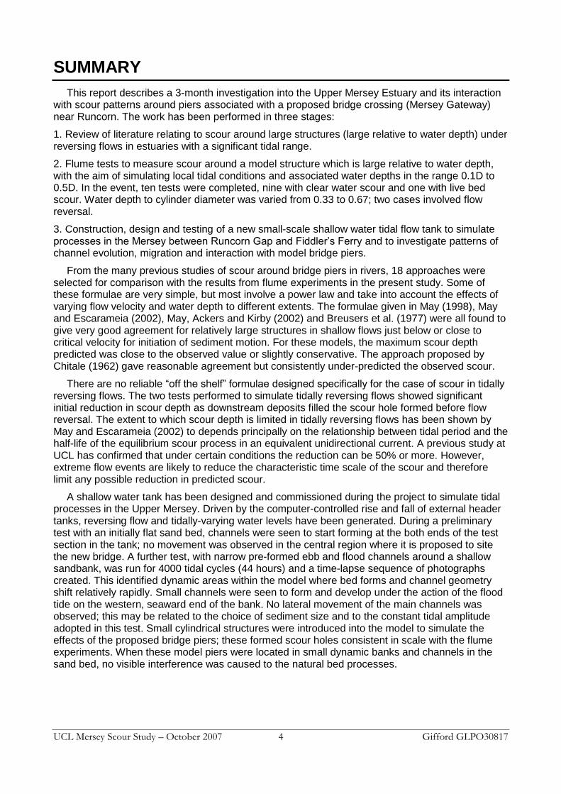
SUMMARY
This report describes a 3-month investigation into the Upper Mersey Estuary and its interaction with scour patterns around piers associated with a proposed bridge crossing (Mersey Gateway) near Runcorn. The work has been performed in three stages:
1. Review of literature relating to scour around large structures (large relative to water depth) under reversing flows in estuaries with a significant tidal range.
2. Flume tests to measure scour around a model structure which is large relative to water depth, with the aim of simulating local tidal conditions and associated water depths in the range 0.1D to 0.5D. In the event, ten tests were completed, nine with clear water scour and one with live bed scour. Water depth to cylinder diameter was varied from 0.33 to 0.67; two cases involved flow reversal.
3. Construction, design and testing of a new small-scale shallow water tidal flow tank to simulate processes in the Mersey between Runcorn Gap and Fiddler‟s Ferry and to investigate patterns of channel evolution, migration and interaction with model bridge piers.
From the many previous studies of scour around bridge piers in rivers, 18 approaches were selected for comparison with the results from flume experiments in the present study. Some of these formulae are very simple, but most involve a power law and take into account the effects of varying flow velocity and water depth to different extents. The formulae given in May (1998), May and Escarameia (2002), May, Ackers and Kirby (2002) and Breusers et al. (1977) were all found to give very good agreement for relatively large structures in shallow flows just below or close to critical velocity for initiation of sediment motion. For these models, the maximum scour depth predicted was close to the observed value or slightly conservative. The approach proposed by Chitale (1962) gave reasonable agreement but consistently under-predicted the observed scour.
There are no reliable “off the shelf” formulae designed specifically for the case of scour in tidally reversing flows. The two tests performed to simulate tidally reversing flows showed significant initial reduction in scour depth as downstream deposits filled the scour hole formed before flow reversal. The extent to which scour depth is limited in tidally reversing flows has been shown by May and Escarameia (2002) to depends principally on the relationship between tidal period and the half-life of the equilibrium scour process in an equivalent unidirectional current. A previous study at UCL has confirmed that under certain conditions the reduction can be 50% or more. However, extreme flow events are likely to reduce the characteristic time scale of the scour and therefore limit any possible reduction in predicted scour.
A shallow water tank has been designed and commissioned during the project to simulate tidal processes in the Upper Mersey. Driven by the computer-controlled rise and fall of external header tanks, reversing flow and tidally-varying water levels have been generated. During a preliminary test with an initially flat sand bed, channels were seen to start forming at the both ends of the test section in the tank; no movement was observed in the central region where it is proposed to site the new bridge. A further test, with narrow pre-formed ebb and flood channels around a shallow sandbank, was run for 4000 tidal cycles (44 hours) and a time-lapse sequence of photographs created. This identified dynamic areas within the model where bed forms and channel geometry shift relatively rapidly. Small channels were seen to form and develop under the action of the flood tide on the western, seaward end of the bank. No lateral movement of the main channels was observed; this may be related to the choice of sediment size and to the constant tidal amplitude adopted in this test. Small cylindrical structures were introduced into the model to simulate the effects of the proposed bridge piers; these formed scour holes consistent in scale with the flume experiments. When these model piers were located in small dynamic banks and channels in the sand bed, no visible interference was caused to the natural bed processes.
UCL Mersey Scour Study – October 2007 5 Gifford GLPO30817
Glossary
Accretion: Process by which particles carried by the flow of water are deposited and accumulated (the opposite of erosion).
Clear-water scour: Scour (normally local scour) where the bed material in the flow upstream of the scour hole is at rest.
Critical flow: Water flow at which the specific energy is a minimum for a given discharge (and Froude number is unity).
Discharge: Flow rate expressed in volume per unit time.
Ebb/ebb tide: Tidal flow associated with falling tide; flow from estuary to sea.
Eddy: Single vertical vortex.
Erosion: Process by which particles are removed by the action of wind, flowing water or waves (the opposite of accretion)
Estuary: Tidal reach at the mouth of a river
Flood/flood tide: Flow of water from the ocean to the bay or estuary.
Froude number: Dimensionless parameter representing the ratio between the inertia and gravity forces in a fluid, taking the value of unity for critical flow.
Local scour: Scour that results directly from the impact of individual structural elements (e.g. piles and abutments) on the flow and occurs only in the immediate vicinity of those elements.
Live-bed scour: Scour (normally local scour) where there is a general movement of bed material, ultimately with a balance between the sediment entering and leaving the scour hole.
Pile: Slender (compared to height) structural member substantially underground intended to transmit forces into load bearing strata below the surface of the land.
Scour: Erosion resulting from the shear forces associated with flowing water and wave action.
Sediment: Fine material transported in a liquid that settles or tends to settle.
Shear stress: Force per unit area exerted by fluid on seabed (due to fluid flow) and acting tangential to its surface in the direction of flow.
Shields criterion: Threshold of movement of particles, expressed in terms of two dimensionless numbers, the entrainment function and the particle Reynolds number, based on experimental work by Shields (and others) on granular sediment.
Spring tides: Tides on the two occasions per lunar month when the predicted range between successive high water and low water is greatest.
Storm surge: Coastal flooding phenomenon resulting from wind and barometric changes. The storm surge is measured by subtracting the astronomical tide elevation from the total flood elevation.
Storm tide: Coastal flooding resulting from combination of storm surge and astronomical tide (often referred to as storm surge).
Tidal cycle: One complete rise and fall of the tide.
Tidal day: Time of rotation of the earth with respect to the moon. Assumed to equal approximately 24.84 solar hours in length.
Tidal inlet: A channel connecting a bay or estuary to the ocean.
Tidal range: Vertical distance between specified low and high tide levels.
Tides: Periodic rising and falling of water resulting from the gravitational attraction of the moon, sun and other astronomical bodies, together with the effects of coastal aspect and bathymetry.
Thalweg: the line of the deepest point of a channel.

UCL Mersey Scour Study – October 2007 6 Gifford GLPO30817
1. Background
The Mersey Estuary is located on the Irish Sea coast of north-west England. It is a large, sheltered estuary, which comprises large areas of salt marsh and extensive intertidal sand- and mud-flats, with limited areas of brackish marsh, rocky shoreline and boulder clay cliffs, within a rural and industrial environment. The intertidal flats and salt marshes provide feeding and roosting sites for large populations of water birds. That is why the Mersey Estuary has been internationally recognised (Ramsar/SPA) and is protected for its valuable bird life.
However, it is home to heavy industry and major ports, as well as residential areas, and the growing traffic in Widnes, Runcorn and within 10km can only cross the Mersey at the Silver Jubilee Bridge. To ease traffic congestion in Widnes and allow the area to develop, the construction of a new road crossing over the Mersey is being planned.
It has been proposed that the bridge is supported on three piers, to be constructed in the Upper Estuary. The introduction of large structures to a sediment bed subjected to tidal currents produces scour; depending on the extent of this scour and any interactions between the structure and flow channels, it could change the habitat of the many species living there.
The role of the UCL Civil, Environmental and Geomatic Engineering Department is to study the impact of the construction of the Mersey Gateway, and to see if it is likely to change the mobile sediment characteristics of the Mersey Upper Estuary. In particular, the aims of the work are:
a) Identify the scour prediction formula best fitting the Mersey Estuary case
b) Carry out experiments on scour around a cylinder in relatively shallow flow
c) Use a small-scale model to study estuary morphology and the effects of piers on it.
Figure 1 Mersey Upper Estuary showing existing bridges at Runcorn (foreground) and the proposed Mersey Gateway bridge (middle distance)- Photo courtesy of Gifford
UCL Mersey Scour Study – October 2007 7 Gifford GLPO30817
2. Scour
This section describes how sediment is transported and how it reacts to an obstacle.
2.1 Definition of scour
Scour is the process where sediment is eroded from an area of the sea bed in response to forcing by waves or currents. There are three common types of scour: “general”, “constriction” and “local” [Whitehouse (1998], Gifford B4027.TR03.04].
2.1.1 General scour
General scour is attributed to natural processes distinct from the interaction of any structure existing on a bed. It can be initiated by distinct events such as floods with an immediate effect on erodible boundary material, or in contrast, it can be attributed to gradual changes such as degradation and aggregation of boundary materials associated with the morphological characteristics of the channel or estuary and its boundary materials.
2.1.2 Constriction scour
Constriction scour is generally caused by a local narrowing often created by the presence of one or more structures such as bridge piers or training works placed in a fluvial or marine bed. The narrowing causes an increase in flow velocity over its length and a corresponding increase in bed shear stress.
2.1.3 Local scour
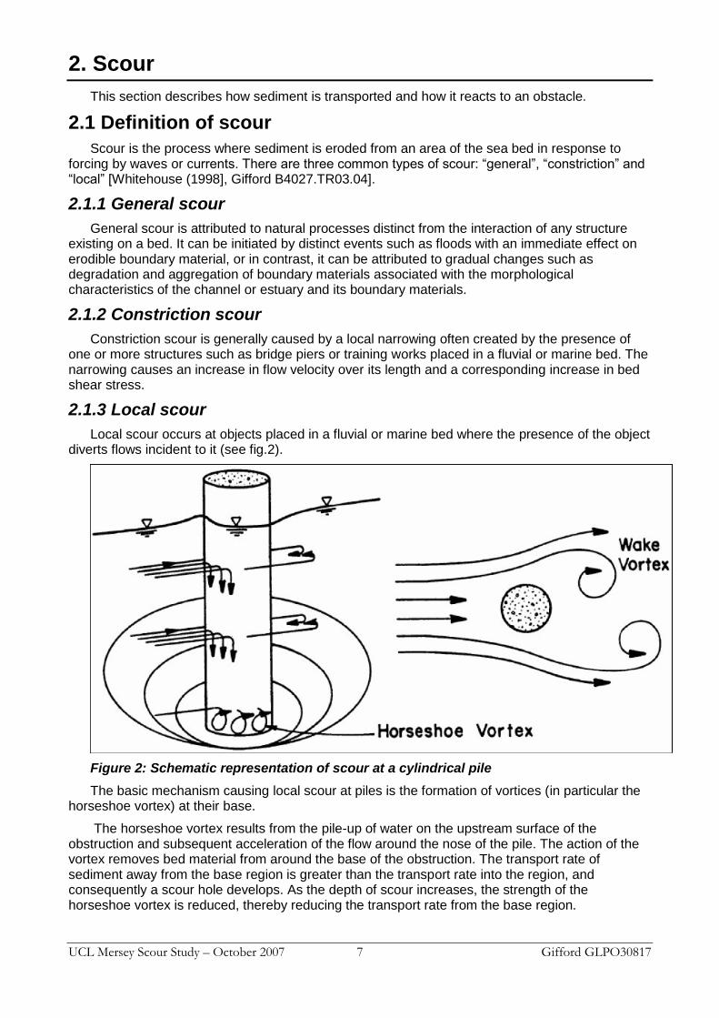
Local scour occurs at objects placed in a fluvial or marine bed where the presence of the object diverts flows incident to it (see fig.2).
Figure 2: Schematic representation of scour at a cylindrical pile
The basic mechanism causing local scour at piles is the formation of vortices (in particular the horseshoe vortex) at their base.
The horseshoe vortex results from the pile-up of water on the upstream surface of the obstruction and subsequent acceleration of the flow around the nose of the pile. The action of the vortex removes bed material from around the base of the obstruction. The transport rate of sediment away from the base region is greater than the transport rate into the region, and consequently a scour hole develops. As the depth of scour increases, the strength of the horseshoe vortex is reduced, thereby reducing the transport rate from the base region.
UCL Mersey Scour Study – October 2007 8 Gifford GLPO30817
In addition to the horseshoe vortex around the base of a pile, there are vertical vortices downstream of the pile called wake vortices. Both the horseshoe and wake vortices remove material from the pile base region.
However, the intensity of wake vortices diminishes rapidly as the distance downstream of the pile increases. Therefore, immediately downstream of a long pile there is often deposit of material.
Factors that affect the depth of local scour at piles are [Morten Sand Jensen et al. (2006)]:
(1) Flow velocity.
(2) Water depth.
(3) Width of the pile.
(4) Length of the pile if skewed to flow.
(5) Size and gradation of bed material.
(6) Shape of the pile (here circular).
(7) Bed configuration.
(8) Marine growth, ice formation or jams and debris.
2.2 Bed shear stress
Sediment transport and scour are driven by bed shear stress. The shear stress To (frictional force exerted by the flow on unit area of bed) is what plucks sand grains off the bed and entrains them in the flow. If the bed shear stress exceeds a threshold value Tcr for a particular grain size and composition, that grain will be lifted from the bed and carried by the flow. If the bed shear stress drops below that threshold value, the entrained grain will drop back to the bed. So the bed shear stress controls whether erosion (removal of grains) or deposition (settling of grains) will occur.
When we introduce a structure in the sediment bed, the flow speed-up adjacent to the structure can amplify the local value of the bed shear stress.
2.3 Clear-water scour and live-bed scour
Two types of local scour can be identified [Whitehouse, 1998]:
Clear-water scour occurs when there is no movement of the bed material in the flow upstream of the pile (shear stress To<Tcr). At the pile, the acceleration of the flow and vortices created by the obstruction of the pile causes the bed material to move (amplification of the bed shear stress in the vicinity of the structure).
Live-bed scour occurs when there is transport of bed material upstream of the pile (shear stress To>Tcr).
Critical velocity is the velocity associated with the initiation of motion, which means that if the velocity upstream of the pile is lower (bigger) than the critical velocity then local scour will be clear-water (live-bed) scour. The critical velocity is determined by the median diameter of the bed material d50 and by the water depth [Morten Sand Jensen et al., 2006]:
2.4 Equilibrium
The equilibrium scour depth is reached when the agitating force due to the flow balances the resistive force of the particles (clear-water) or when the quantity of sediment removed by local scour is equivalent to the quantity of suspended sediment supplied to the hole from the live bed upstream of the structure (live-bed).
UCL Mersey Scour Study – October 2007 9 Gifford GLPO30817
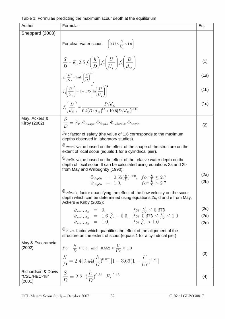
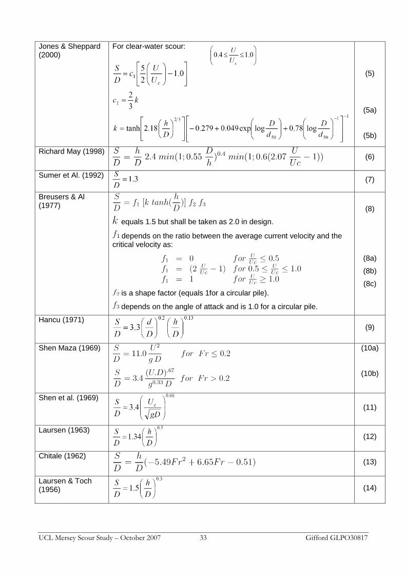
Many formulae have been developed for the estimation of local scour around a cylindrical structure in a uniform current. These are set out in specialist texts on the subject – see, for example, Hoffmans and Verheij (1997), Whitehouse (1998), May et al. (2002), http://www.fhwa.dot.gov/engineering/hydraulics/pubs/03052/05.cfm. Table 1 gives a non-exhaustive list of equations for estimation of scour depth that are in common use and were used during the study. Some of these are for the simplest case where depth of scour relates only to the size of the structure. Others are more complex, relating scour to the flow velocity relative to critical velocity (threshold of sediment movement), water depth relative to size of the structure, sediment characteristics, and shape and orientation of the structure. Most formulae have been developed to match small-scale laboratory tests, and it is suggested that results from such tests are likely to be conservative in comparison to field observations. A reliable formula is one that predicts close to observed values but errs only by over-predicting the extent of scour.
2.5 Scour in tidal flows
The process of scour requires a significant length of time for an equilibrium state to develop in the scour hole. This relies on a continuous flow being maintained for the equilibrium conditions to exist. The report Case study of bridges constructed in highly mobile estuaries or river beds [Gifford, B4027/TR03/04] explains that an object in a tidal flow regime such as the proposed bridge piers of the New Mersey Crossing is not subject to a steady flow but a constantly changing flow which reverses in direction approximately twice daily. Tidal flow magnitudes also vary between spring and neap cycles and extreme tidal and fluvial events.
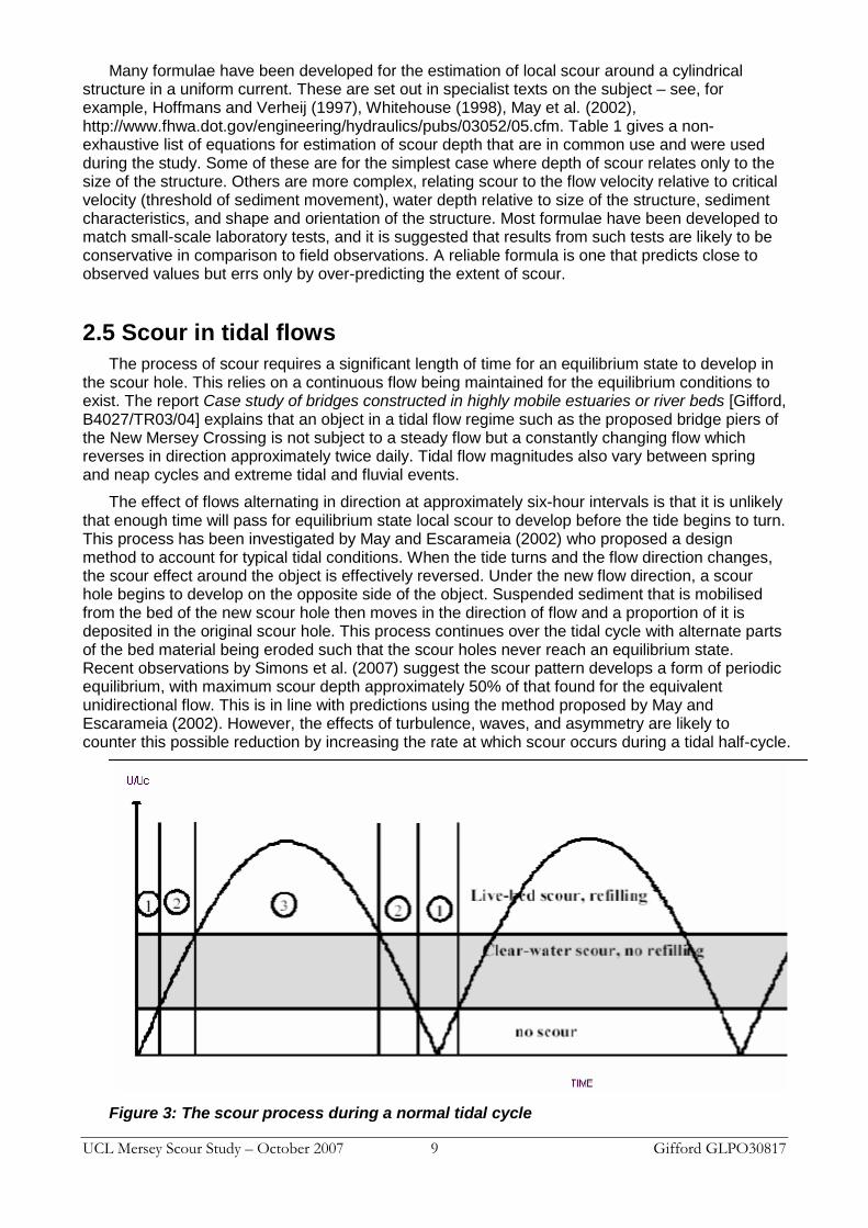
The effect of flows alternating in direction at approximately six-hour intervals is that it is unlikely that enough time will pass for equilibrium state local scour to develop before the tide begins to turn. This process has been investigated by May and Escarameia (2002) who proposed a design method to account for typical tidal conditions. When the tide turns and the flow direction changes, the scour effect around the object is effectively reversed. Under the new flow direction, a scour hole begins to develop on the opposite side of the object. Suspended sediment that is mobilised from the bed of the new scour hole then moves in the direction of flow and a proportion of it is deposited in the original scour hole. This process continues over the tidal cycle with alternate parts of the bed material being eroded such that the scour holes never reach an equilibrium state. Recent observations by Simons et al. (2007) suggest the scour pattern develops a form of periodic equilibrium, with maximum scour depth approximately 50% of that found for the equivalent unidirectional flow. This is in line with predictions using the method proposed by May and Escarameia (2002). However, the effects of turbulence, waves, and asymmetry are likely to counter this possible reduction by increasing the rate at which scour occurs during a tidal half-cycle.
Figure 3: The scour process during a normal tidal cycle
UCL Mersey Scour Study – October 2007 10 Gifford GLPO30817
In the Upper Mersey Estuary, there tends to be a greater flood velocity than ebb velocity. Higher velocity will prevail on the flood tide, which means that the bed shear stress at the pier structure will be more amplified than on the ebb tide. This could therefore lead to a deeper scour hole created by the flood than the ebb flow. In the upper estuary, the ebb lasts for far longer than the flood and therefore, in contrast with the theory above, if the bed shear stress is exceeded at a relatively low velocity, it may be that the longer ebb flow could result in a deeper scour hole than the flood flow as it has more time to develop. So, depending on which flow is dominant in the development of scour, we will obtain an asymmetric shape of scour hole.
In general the scour process under a typical tide condition is illustrated in Fig. 3.
3. Flume experiments
This section describes the set of experiments that were carried out to improve our knowledge of scour around a circular cylinder in relatively shallow water.
3.1 Apparatus and measurement techniques
3.1.1 Wave-current flume:
Tests to investigate scour around a cylinder in relatively shallow water were carried out in the wave-current flume in the Pat Kemp Fluids Laboratory at UCL. Water is supplied to the flume from header tanks in the Chadwick Building roof-space through pipes, and it discharges into a sump below the laboratory floor. Water is re-circulated from the sump to the roof-tanks using two pumps in the Pump Room; these are controlled by a monitoring system with sensors in both high- and low-level tanks.
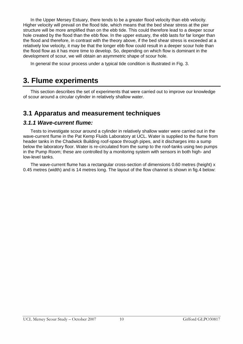
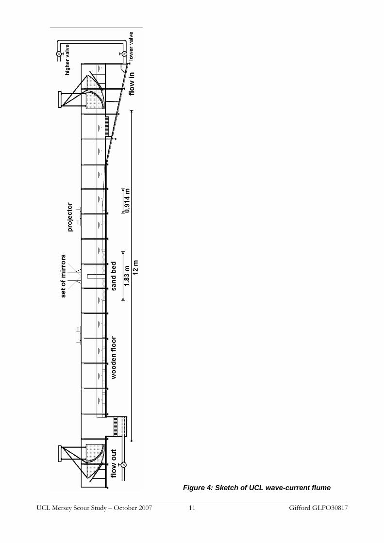
The wave-current flume has a rectangular cross-section of dimensions 0.60 metres (height) x 0.45 metres (width) and is 14 metres long. The layout of the flow channel is shown in fig.4 below:
UCL Mersey Scour Study – October 2007 11 Gifford GLPO30817
Figure 4: Sketch of UCL wave-current flume
UCL Mersey Scour Study – October 2007 12 Gifford GLPO30817
Two valves are used to control the flow at the inlet. The higher one opens the pipe coming from the roof, and the lower opens directly into the inlet of the flume. This system allows flexible adjustment of the flow rate. During the present experiments, the higher valve was opened fully to let in the required flow rate.
So, maintaining the same depth and lower inlet valve settings, it is possible to reproduce the same flow velocity in the flume.
One valve closes the outlet tank. When it is closed, it allows the outlet tank to fill up slowly, making it possible to interrupt an experiment without emptying the flume, and to start it again later without disrupting the scour patterns.
At the outlet end of the flume, there is an adjustable weir gate. This can be adjusted from 0 to 12 cm. By adjusting the height of the weir gate and the velocity with the lower valve, it is possible to set up the required water depth.
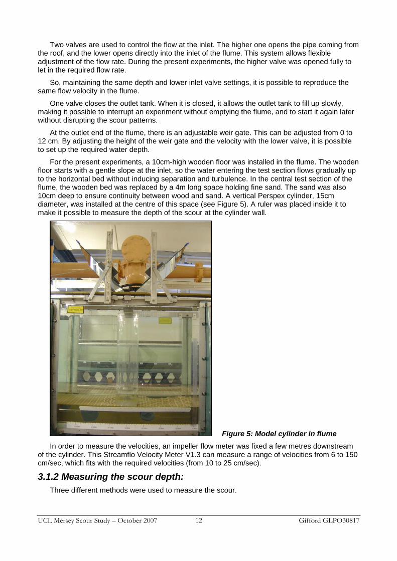
For the present experiments, a 10cm-high wooden floor was installed in the flume. The wooden floor starts with a gentle slope at the inlet, so the water entering the test section flows gradually up to the horizontal bed without inducing separation and turbulence. In the central test section of the flume, the wooden bed was replaced by a 4m long space holding fine sand. The sand was also 10cm deep to ensure continuity between wood and sand. A vertical Perspex cylinder, 15cm diameter, was installed at the centre of this space (see Figure 5). A ruler was placed inside it to make it possible to measure the depth of the scour at the cylinder wall.
Figure 5: Model cylinder in flume
In order to measure the velocities, an impeller flow meter was fixed a few metres downstream of the cylinder. This Streamflo Velocity Meter V1.3 can measure a range of velocities from 6 to 150 cm/sec, which fits with the required velocities (from 10 to 25 cm/sec).
3.1.2 Measuring the scour depth:
Three different methods were used to measure the scour.
UCL Mersey Scour Study – October 2007 13 Gifford GLPO30817
a) Pointer:
A pointer made with a metal rod was mounted on a trolley above the sand bed. The pointer could be traversed across the Y axis (across the flume), and the trolley could be moved along the X axis (along the flume).
Advantages: Can be used whatever the water depth is;
Precise;
Can be used while flowing (does not introduce noticeable disturb to the flow);
Can reach every part of the scoured bed.
Drawbacks: Extremely slow to measure an area.
b) Laser pointer with projected grid:
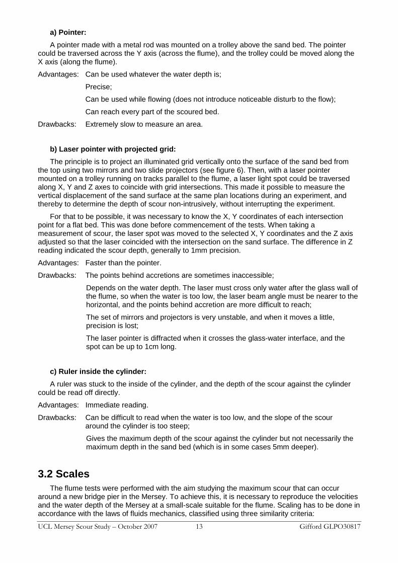
The principle is to project an illuminated grid vertically onto the surface of the sand bed from the top using two mirrors and two slide projectors (see figure 6). Then, with a laser pointer mounted on a trolley running on tracks parallel to the flume, a laser light spot could be traversed along X, Y and Z axes to coincide with grid intersections. This made it possible to measure the vertical displacement of the sand surface at the same plan locations during an experiment, and thereby to determine the depth of scour non-intrusively, without interrupting the experiment.
For that to be possible, it was necessary to know the X, Y coordinates of each intersection point for a flat bed. This was done before commencement of the tests. When taking a measurement of scour, the laser spot was moved to the selected X, Y coordinates and the Z axis adjusted so that the laser coincided with the intersection on the sand surface. The difference in Z reading indicated the scour depth, generally to 1mm precision.
Advantages: Faster than the pointer.
Drawbacks: The points behind accretions are sometimes inaccessible;
Depends on the water depth. The laser must cross only water after the glass wall of the flume, so when the water is too low, the laser beam angle must be nearer to the horizontal, and the points behind accretion are more difficult to reach;
The set of mirrors and projectors is very unstable, and when it moves a little, precision is lost;
The laser pointer is diffracted when it crosses the glass-water interface, and the spot can be up to 1cm long.
c) Ruler inside the cylinder:
A ruler was stuck to the inside of the cylinder, and the depth of the scour against the cylinder could be read off directly.
Advantages: Immediate reading.
Drawbacks: Can be difficult to read when the water is too low, and the slope of the scour around the cylinder is too steep;
Gives the maximum depth of the scour against the cylinder but not necessarily the maximum depth in the sand bed (which is in some cases 5mm deeper).
3.2 Scales
The flume tests were performed with the aim studying the maximum scour that can occur around a new bridge pier in the Mersey. To achieve this, it is necessary to reproduce the velocities and the water depth of the Mersey at a small-scale suitable for the flume. Scaling has to be done in accordance with the laws of fluids mechanics, classified using three similarity criteria:

UCL Mersey Scour Study – October 2007 14 Gifford GLPO30817
(i) Geometrical similarity
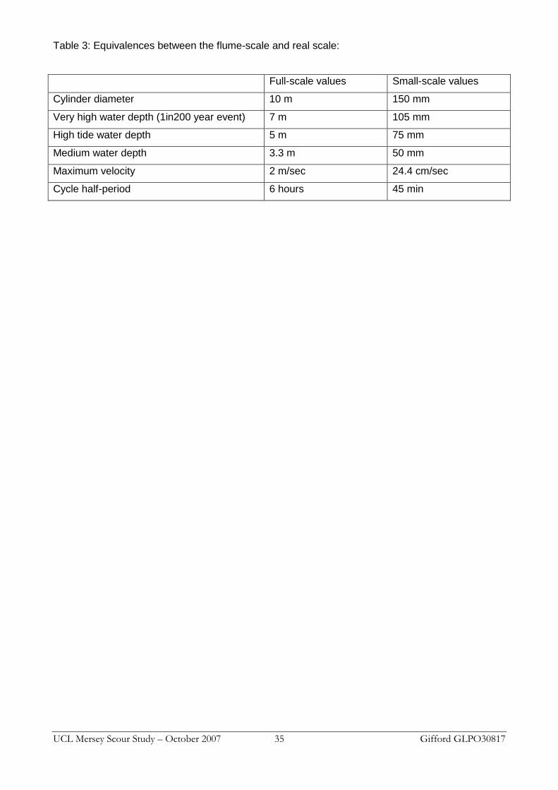
All the linear dimensions of the prototype must be the same as the model, using a constant scale factor. For our case, we chose a scale of 1/67, chosen largely to match the dimensions of the flume and the cylinder. The table 3 gives some equivalence between real and scaled values.
(ii) Kinematic similarity
The fluid flow in both the model and prototype must follow similar patterns and have equivalent values related by a constant scale factor (hence fluid streamlines are similar).
(iii) Dynamic similarity
Ratios of all forces acting on corresponding fluid particles and boundary surfaces in the two systems are constant.
(iv) Similarity conditions deduced from fluid mechanics equations
From the dimensionless equations of Navier-Stokes for an incompressible flow with a free surface, we have:
The similarity of the equations of Navier-Stokes is obtained if we have simultaneously:
In practice, it is not possible to respect both conditions. The gravity forces are significant because this is what carries away the sand. And, when the Reynolds number is greater than a critical value, the flow characteristics are far less sensitive to. That is why the Froude number scaling is commonly adopted for scour studies. Following this approach, the relationship between velocity in the flume and the real velocity in the Mersey is:
3.3 Test procedure
The Mersey Upper Estuary is subject to important variations of water depth and velocity imposed by the tides and surge events. To investigate the deepest scour depth that may occur around a pier of the proposed Mersey Gateway, tests were performed for a range of conditions as listed in the table 2.
3.3.1 Experimental procedure
(i) Three steps to launch an experiment:
Initial adjustment of the velocity and water depth for specific test case: Open fully the higher valve
Adjust the lower valve and the weir gate height iteratively to obtain the required velocity and water depth (this can take a few minutes to stabilize)
Close the higher valve completely
UCL Mersey Scour Study – October 2007 15 Gifford GLPO30817
Smoothing of the sand bed: Empty the water from the flume (open the smaller valve at the inlet, and push the water out
with the scraper at the outlet)
Add sand around the cylinder and also at both ends of the sand bed
Use the larger rake (same length as the flume width) to smooth the bed upstream and downstream of the cylinder, move the excess at both ends onto the wooden bed
Use the smaller rake to smooth around the cylinder, push the excess upstream and downstream
Use the larger rake again to remove the excess around the cylinder, and push all the excess on the wooden floor at both ends
Remove the surplus of sand
Filling of the flume for an experiment: Open the higher valve very slowly until the water flows above the weir gate
Then open the higher valve fully
Check the stabilized velocity and water depth
(ii) Interruption of an experiment:
It was necessary to interrupt experiments at the end of a working day. The following procedure was adopted.
Preparation to stop the experiment: Close the outlet valve
Wait for the tank at the outlet to fill up
Close the higher valve rapidly before the water level in the outlet tank reaches the weir gate
Continue to fill up the flume slowly to achieve 1cm more than the experiment water depth (take into consideration that the spaces under the wooden floor can fill up)
Preparation to continue the experiment: Open the outlet valve to empty the tank
When the water level in the tank is below the weir gate (the flume is starting to empty), open the higher valve fully
Check the stabilized velocity and water depth
3.3.2 Results
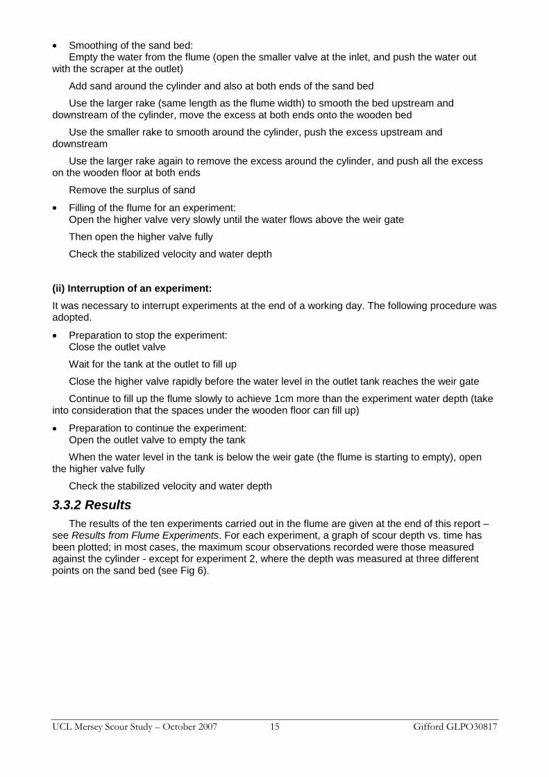
The results of the ten experiments carried out in the flume are given at the end of this report – see Results from Flume Experiments. For each experiment, a graph of scour depth vs. time has been plotted; in most cases, the maximum scour observations recorded were those measured against the cylinder - except for experiment 2, where the depth was measured at three different points on the sand bed (see Fig 6).
UCL Mersey Scour Study – October 2007 16 Gifford GLPO30817
Figure 6: Location of grid intersections on sand bed
3.3.3 Sources of error
Errors are related to the different measurement techniques (see 3.1.2). The measurement of velocity can also be influenced by vortices downstream of the cylinder, even when the position was chosen to minimize such effects. The interruption of flow and possible cementing or slumping of the sand bed during the breaks (overnight or for a weekend) could also have introduced errors: the sand bed can solidify and cohesion between the sand grains can make them more difficult to move. Unforeseen and unknown events can also occur, as experienced in experiment 6 (see 3.3.4).
If the graph of scour depth vs. time is smooth, undisrupted and asymptotic, then it is likely that the experiment has passed without significant error. Recording the velocity at each measurement of scour depth ensured that the tests were performed with a constant flow rate.
3.3.4 Discussion
Experiments 1 to 4 were carried out to determine the capability of the flume to produce velocities and water depths relevant to the Mersey case study.
The velocity for experiments 1 and 2 was approximately half of the critical velocity. Some formulae predicting the maximum scour depth at equilibrium - such as those of Breusers et al. (1977), and May & Escameira (2002) - estimate that, if the velocity is less than half of the critical velocity, then there is no scour. In the present tests, the relatively small depth of scour observed at these low velocities was generated by natural ripples in the sand bed and the depth recorded around the cylinder was not significantly greater than the depth in the trough of some ripples. In effect, the velocity was not strong enough to initiate local scour. However, it was noted that the maximum scour depth was greater for the deeper water case, as predicted by the theory.
In experiments 3 and 4, the velocity was greater than and equal to the critical velocity respectively. In such live-bed conditions, the scour depth increased quickly and reached the bottom of the sand bed before reaching equilibrium. In those cases, the velocities were too high for the flume, cylinder and sediment combination.
UCL Mersey Scour Study – October 2007 17 Gifford GLPO30817
From these test results it was decided to adopt a range of velocities greater than half of the critical velocity and less than the critical velocity.
Experiment 5, with a velocity equals to 17.4cm/sec (80% of critical velocity) and a water depth of 75mm, was continued for 44 hours. The aim was to run the test until it achieved an equilibrium scour depth. After 8 hours, scour depth against the cylinder wall had stabilized at 75 mm, and it was concluded that equilibrium had been reached.
The ratio between scour depth and cylinder diameter, S/D, obtained at equilibrium was S/D=0.513. Among the predictive formulae, the closest to this result are May (1998) and May & Escameira (2002) with ratios S/D=0.494 and S/D=0.538 respectively.
In order to highlight the influence of water depth on the scour depth, the water depth chosen for experiments 6 and 7 was 50 mm. Experiment 6 started from a flat bed, whereas experiment 7 started from the reversed pattern of the scour observed at the end of experiment 6. Results from both experiment showed unexpected behaviour suggesting that the results were not reliable.
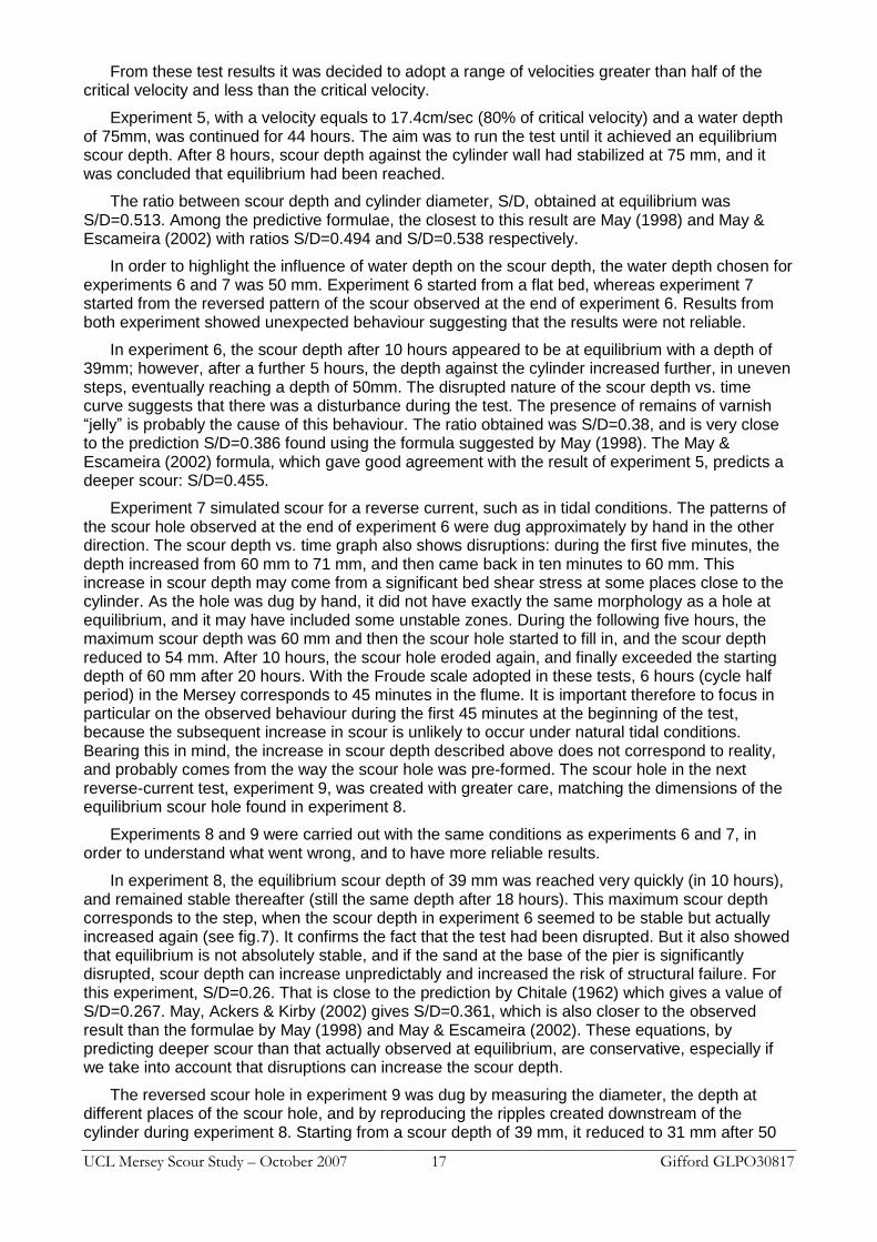
In experiment 6, the scour depth after 10 hours appeared to be at equilibrium with a depth of 39mm; however, after a further 5 hours, the depth against the cylinder increased further, in uneven steps, eventually reaching a depth of 50mm. The disrupted nature of the scour depth vs. time curve suggests that there was a disturbance during the test. The presence of remains of varnish “jelly” is probably the cause of this behaviour. The ratio obtained was S/D=0.38, and is very close to the prediction S/D=0.386 found using the formula suggested by May (1998). The May & Escameira (2002) formula, which gave good agreement with the result of experiment 5, predicts a deeper scour: S/D=0.455.
Experiment 7 simulated scour for a reverse current, such as in tidal conditions. The patterns of the scour hole observed at the end of experiment 6 were dug approximately by hand in the other direction. The scour depth vs. time graph also shows disruptions: during the first five minutes, the depth increased from 60 mm to 71 mm, and then came back in ten minutes to 60 mm. This increase in scour depth may come from a significant bed shear stress at some places close to the cylinder. As the hole was dug by hand, it did not have exactly the same morphology as a hole at equilibrium, and it may have included some unstable zones. During the following five hours, the maximum scour depth was 60 mm and then the scour hole started to fill in, and the scour depth reduced to 54 mm. After 10 hours, the scour hole eroded again, and finally exceeded the starting depth of 60 mm after 20 hours. With the Froude scale adopted in these tests, 6 hours (cycle half period) in the Mersey corresponds to 45 minutes in the flume. It is important therefore to focus in particular on the observed behaviour during the first 45 minutes at the beginning of the test, because the subsequent increase in scour is unlikely to occur under natural tidal conditions. Bearing this in mind, the increase in scour depth described above does not correspond to reality, and probably comes from the way the scour hole was pre-formed. The scour hole in the next reverse-current test, experiment 9, was created with greater care, matching the dimensions of the equilibrium scour hole found in experiment 8.
Experiments 8 and 9 were carried out with the same conditions as experiments 6 and 7, in order to understand what went wrong, and to have more reliable results.
In experiment 8, the equilibrium scour depth of 39 mm was reached very quickly (in 10 hours), and remained stable thereafter (still the same depth after 18 hours). This maximum scour depth corresponds to the step, when the scour depth in experiment 6 seemed to be stable but actually increased again (see fig.7). It confirms the fact that the test had been disrupted. But it also showed that equilibrium is not absolutely stable, and if the sand at the base of the pier is significantly disrupted, scour depth can increase unpredictably and increased the risk of structural failure. For this experiment, S/D=0.26. That is close to the prediction by Chitale (1962) which gives a value of S/D=0.267. May, Ackers & Kirby (2002) gives S/D=0.361, which is also closer to the observed result than the formulae by May (1998) and May & Escameira (2002). These equations, by predicting deeper scour than that actually observed at equilibrium, are conservative, especially if we take into account that disruptions can increase the scour depth.
The reversed scour hole in experiment 9 was dug by measuring the diameter, the depth at different places of the scour hole, and by reproducing the ripples created downstream of the cylinder during experiment 8. Starting from a scour depth of 39 mm, it reduced to 31 mm after 50
UCL Mersey Scour Study – October 2007 18 Gifford GLPO30817
0
10
20
30
40
50
0 5 10 15 20 25
Time (hours)
Sco
ur
dep
th a
gain
st
the c
yli
nd
er
(mm
)
Experiment 6 Experiment 8
Figure 7: Comparison of two experiments performed with the same parameters (50 mm water depth, 17.4 cm/sec velocity)
minutes. After 1.4 hour, the scour depth increased but never exceeded the starting scour depth, even after 18 hours. These results correspond to the theory that when the current direction changes, the scour hole fills up, and is then eroded again. Observations after 45 minutes at the beginning of the test show that the changing of direction of the currents in a tidal system does not make the scour depth any greater than the initial (previous) equilibrium scour depth for an equivalent unidirectional flow. The tidal half cycle is not long enough to allow the scour depth to reach equilibrium. That is why, in these conditions of water depth and velocity, if we start from a flat bed (and not from equilibrium, which would be the worse case), we can assume that the tidal currents would never create a scour hole as great as the unidirectional equilibrium value. The maximum scour depth achievable would be less than the conventional equilibrium scour depth.
UCL Mersey Scour Study – October 2007 19 Gifford GLPO30817
To highlight the influence of the velocity on scour depth evolution, a test was performed with a lower velocity (15cm/sec, 75% of the critical velocity), but with the same water depth. Experiment 10 gave a ratio S/D=0.30. The closest prediction was from Breusers et al. (1977), which predicts S/D=0.323. May (1998) is also close to the result, but predicts less scour depth: S/D=0.266. May & Escameira (2002) give a good prediction of scour depth, with S/D=0.346.
3.3.5 Comparisons
Some formulae predicting the maximum scour depth do not include the water depth, or the velocity. In order to determine the equations which fit best to the study of scour around a cylinder in shallow water depth, it is important to know the influence of those factors on the scour depth.
(i) Water depth:
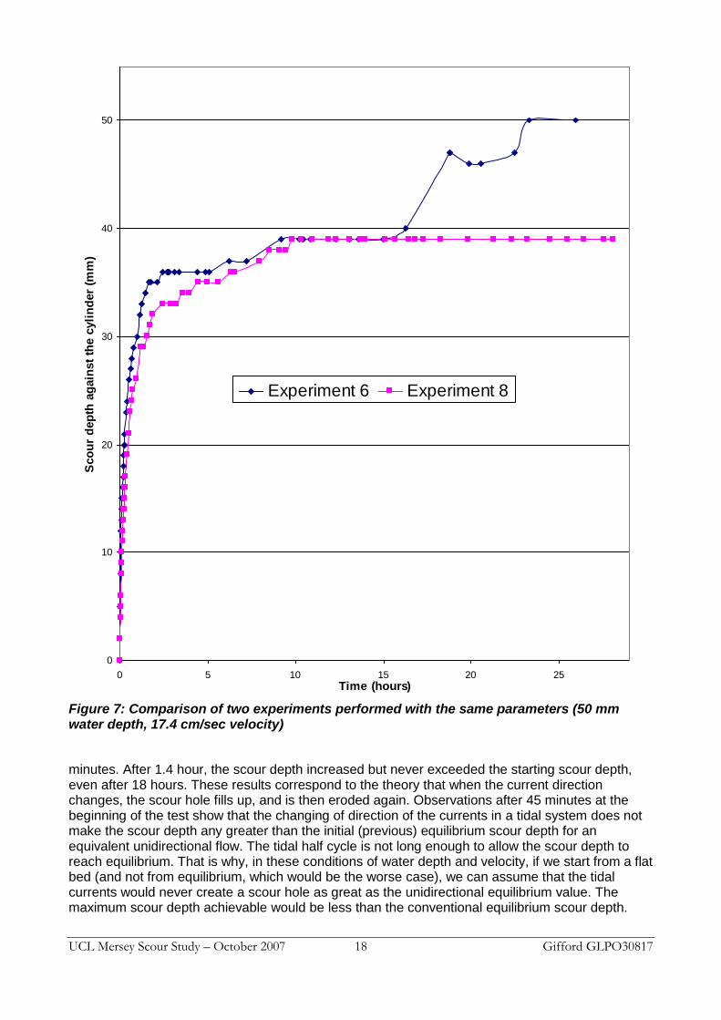
Experiments 5 and 8 (see Figure 8) were carried out with the same velocity (17.4 cm/sec) and two different water depths: 75 mm (1/2 D) and 50 mm (1/3 D). The graph confirms predictions that scour is deeper with a greater water depth. The difference between the two equilibrium scour depths, equivalent to 1/4 D, is significant. It can be deduced that water depth is important in the calculation of scour depth predictions and must be taken into account in the formulae.
It is also notable that both graphs of scour depth vs. time have nearly the same slope at the origin. However the test with the lower water depth reaches equilibrium in just 10 hours whereas the test with the greater water depth takes 36 hours to reach equilibrium.
(ii) Velocity:
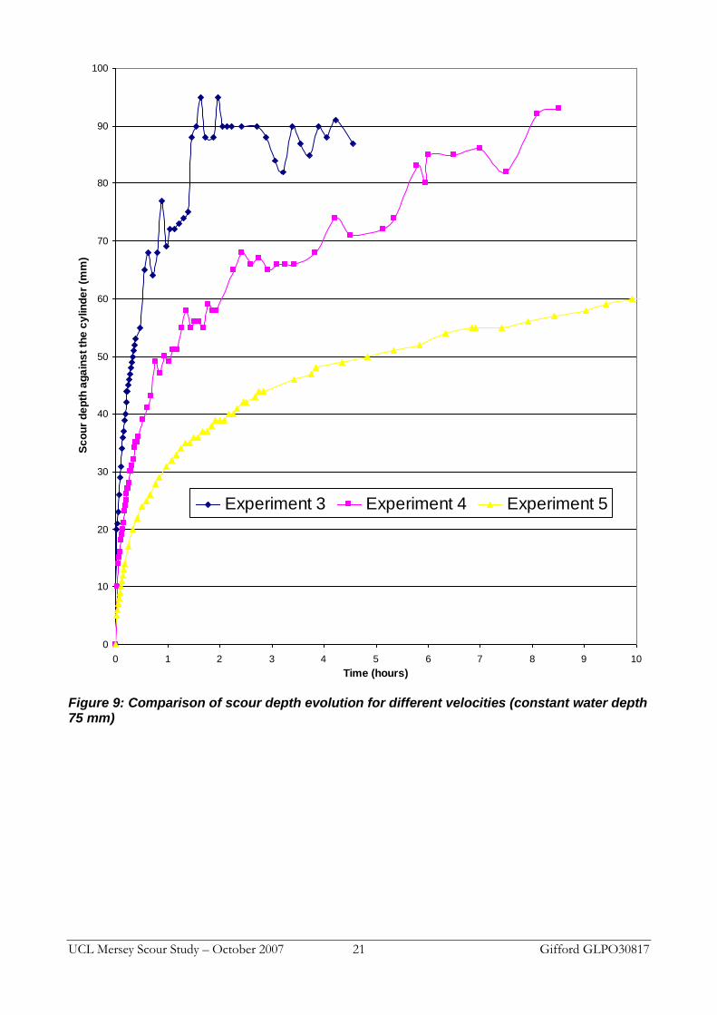
Experiment 3, 4 and 5 (see fig.9), were carried out with a constant water depth (75 mm) and three different velocities: 24.4 cm/sec (1.14 Uc), 21 cm/sec (Uc) and 17.4 cm/sec (0.81 Uc). The tests in live-bed conditions could not be continued through to equilibrium, but fig.9 shows the development of scour during the first few hours. The tangents at the origin have a different slope. As expected, the slope is greater for the higher velocities, and it can reasonably be assumed that if the tests could have been continued until equilibrium, the scour depths would differ significantly.
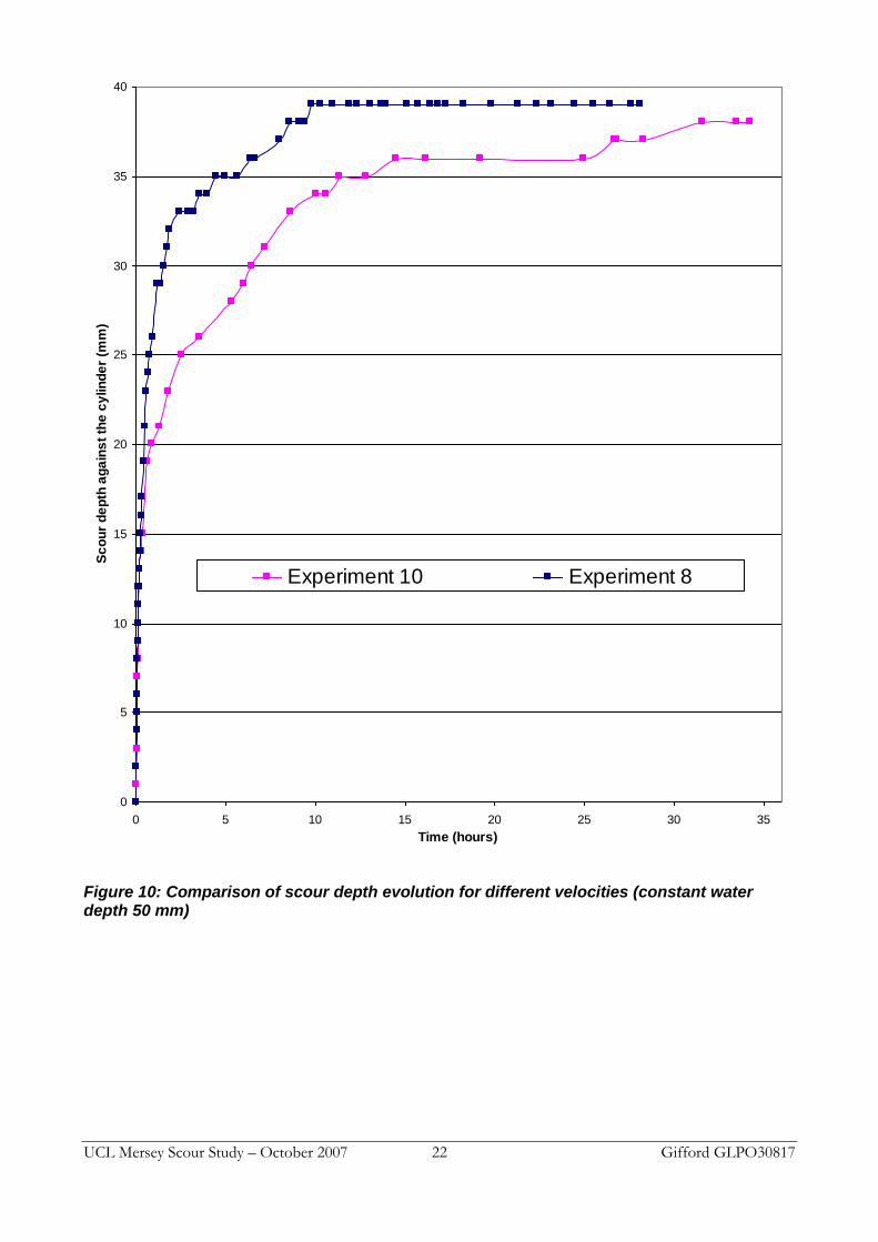
Experiments 8 and 10 (see fig.10) were carried out with a lower water depth (50 mm) than previously and with two different velocities: 17.4 cm/sec (0.87 Uc) and 15 cm/sec (0.75 Uc). The results are surprising because the maximum scour depth at equilibrium is greater for the lower velocity (S/D=0.30 for experiment 10 and S/D=0.26 for experiment 8). The tangents at the origin are quite similar, but then the curves behave as expected: when the scour depth exceeds 20 mm, the rate of scour for the case with the lowest velocity decreases relative to the faster flow. But the test with the high velocity reaches equilibrium after 10 hours whereas the slower flow case continues to scour. However, it can be seen that experiment 10 shows a constant step at S=36mm after 26 hours. It is possible that the same disruption may be occurring as seen in experiment 6.
3.4 Conclusion
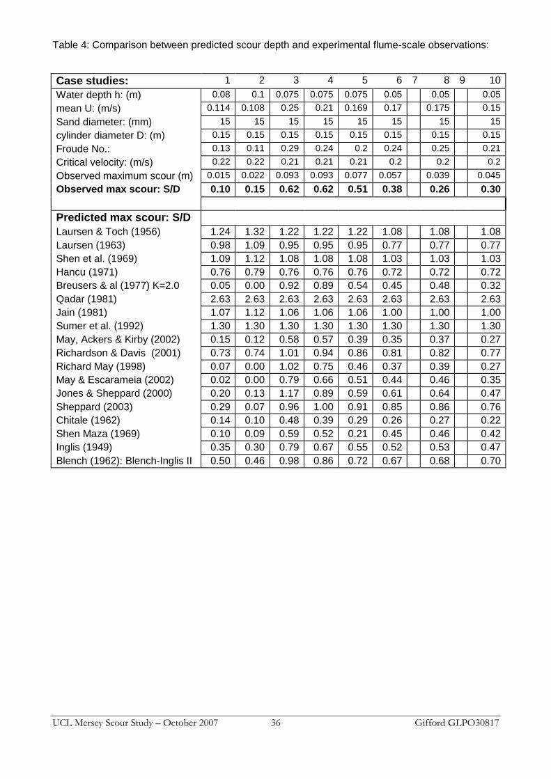
Predictions from 18 different formulae listed in Table 1, including those referred to above, are shown in Table 4. The values that fit best to the results are those using formulae from May (1998) and May & Escameira (2002). Predictions using May, Ackers & Kirby (2002) and Breusers et al. (1977) were also close to the results. All these formulae take into account the water depth and the velocity. Any of these four approaches should provide a conservative prediction for equilibrium scour depth. Results from the tests with current direction reversed confirm observations from previous studies that scour is reduced under certain specific tidal conditions; the method proposed by May and Escarameia (2002) provides an estimate of this reduction. However, the effects of turbulence, waves and extreme storm events will largely counter this effect and it is recommended not to make any such reduction to account for tidal reversal in the Mersey.Estuary.
UCL Mersey Scour Study – October 2007 20 Gifford GLPO30817
0
10
20
30
40
50
60
70
80
0 5 10 15 20 25 30 35 40 45
Time (hours)
Sc
ou
r d
ep
th a
ga
ins
t th
e c
ylin
de
r (m
m)
Experiment 8 Experiment 5
Figure 8: Comparison of scour depth evolution for different water depths (constant velocity 17.4 cm/sec)
UCL Mersey Scour Study – October 2007 21 Gifford GLPO30817
0
10
20
30
40
50
60
70
80
90
100
0 1 2 3 4 5 6 7 8 9 10
Time (hours)
Sc
ou
r d
ep
th a
ga
ins
t th
e c
ylin
de
r (m
m)
Experiment 3 Experiment 4 Experiment 5
Figure 9: Comparison of scour depth evolution for different velocities (constant water depth 75 mm)
UCL Mersey Scour Study – October 2007 22 Gifford GLPO30817
0
5
10
15
20
25
30
35
40
0 5 10 15 20 25 30 35
Time (hours)
Sc
ou
r d
ep
th a
ga
ins
t th
e c
ylin
de
r (m
m)
Experiment 10 Experiment 8
Figure 10: Comparison of scour depth evolution for different velocities (constant water depth 50 mm)
UCL Mersey Scour Study – October 2007 23 Gifford GLPO30817
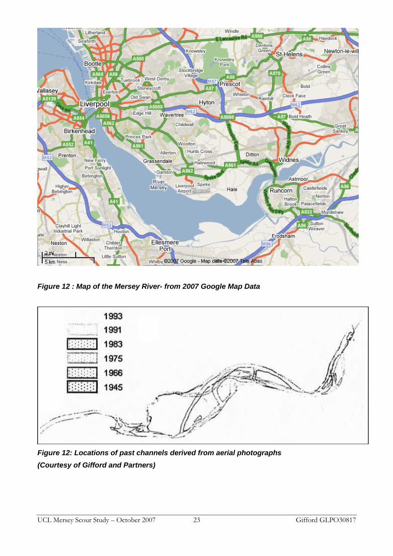
Figure 12 : Map of the Mersey River- from 2007 Google Map Data
Figure 12: Locations of past channels derived from aerial photographs
(Courtesy of Gifford and Partners)
UCL Mersey Scour Study – October 2007 24 Gifford GLPO30817
4. Mini model of the Upper Mersey Estuary
The Upper Estuary of the Mersey between Runcorn and Astmoor (see Figure 11) typically exhibits two distinct but mobile channels. These are clearly visible at low water. The development and range of movement of these channels can be seen in figure 12, which shows the locations of past channels.
The proposed New Mersey Gateway Crossing will consist of a major bridge with long approach viaducts. This alignment will include a number of bridge piers and major bridge towers within the breadth of the estuary, several of which will need to be constructed in the area of highly mobile sediment within the estuary.
The mobile characteristic of the Upper Estuary is a major issue, and concern has been expressed that the proposed bridge may have a permanent impact. In particular, loss of mobility of the two channels or the permanent attachment of either to the bridge piers would be seen as a significant detrimental impact. Further, if the structure diverted either channel to cause it to „fix‟ to the lateral limits of the existing pattern of channels, thus increasing the rate of erosion of the salt marsh, this would also be unacceptable.
In order to determine the impacts of the proposed structure on the Upper Estuary, computer modelling has been carried out by ABPMer. However, the results of these model tests showed that the general variability in channel form and position observed in nature cannot readily be reproduced. The report Additional Modelling – Mersey Gateway. Technical Note C: Flat Bed Morphological Modelling (Gifford, R.1241c, 2005) explains that the model wants to move towards an equilibrium form based on the forcing conditions and sediment properties applied. Once this profile has developed, very little change occurs. That is why it is not possible to use these models to predict the likelihood of a channel attaching to the bridge piers.
The aim of the research is to investigate any processes through which a thalweg (the line of the deepest point of a channel) and thus the line of a channel itself could become attached to the bridge piers. The work started with the six objectives:
(i) Starting from a flat bed, how far can the channels form from the outlet and inlet?
(ii) What is the long term behaviour of the natural channels?
(iii) What is the effect of the piers on the natural channels?
(iv) What is the effect of the spring-neap system?
(v) What is the effect of a fluvial storm event?
(vi) What is the effect of a storm surge and tide?
4.1 Design and construction of the tidal model
Over the past 120 years, small scale models have been used to a greater or lesser extent to provide an insight into the behaviour of complex coastal and estuary systems. Some of the first engineers to make extensive use of such models were Reynolds (1887) and Vernon Harcourt (1890). By coincidence, both used them to investigate the Mersey estuary. Gibson (1930) and others in the early 20th century developed techniques for constructing very small-scale hydraulic models, and their use continued for many years despite the advent of more advanced techniques for large scale physical modelling and an increasing adherence to the rules of scaling laws. Mann and Stevenson (1995) questioned the use of heavily distorted scales for mobile bed models, also emphasizing the importance of selecting an appropriate bed material. They commented on the lack of validation for many such models and concluded that, where practical, large-scale models were preferable for mobile bed studies. However, they did concede that mini models have in some cases been very successful in simulating aspects of bed movement when compared with natural survey data.
UCL Mersey Scour Study – October 2007 25 Gifford GLPO30817
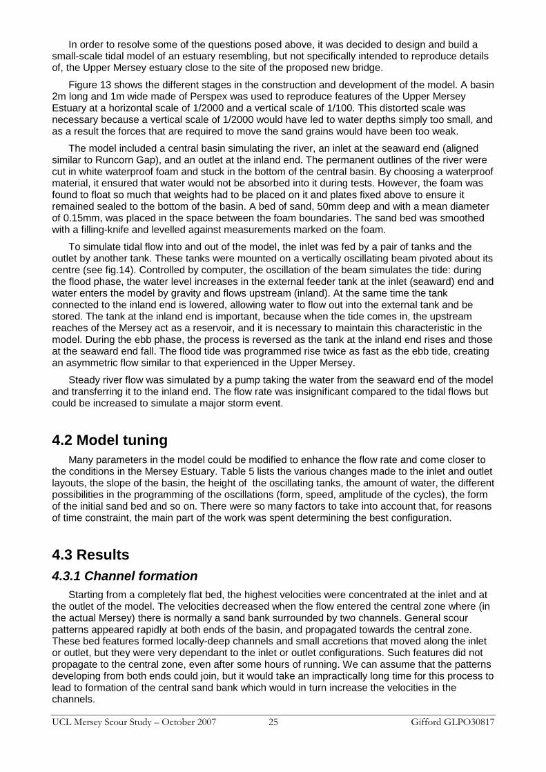
In order to resolve some of the questions posed above, it was decided to design and build a small-scale tidal model of an estuary resembling, but not specifically intended to reproduce details of, the Upper Mersey estuary close to the site of the proposed new bridge.
Figure 13 shows the different stages in the construction and development of the model. A basin 2m long and 1m wide made of Perspex was used to reproduce features of the Upper Mersey Estuary at a horizontal scale of 1/2000 and a vertical scale of 1/100. This distorted scale was necessary because a vertical scale of 1/2000 would have led to water depths simply too small, and as a result the forces that are required to move the sand grains would have been too weak.
The model included a central basin simulating the river, an inlet at the seaward end (aligned similar to Runcorn Gap), and an outlet at the inland end. The permanent outlines of the river were cut in white waterproof foam and stuck in the bottom of the central basin. By choosing a waterproof material, it ensured that water would not be absorbed into it during tests. However, the foam was found to float so much that weights had to be placed on it and plates fixed above to ensure it remained sealed to the bottom of the basin. A bed of sand, 50mm deep and with a mean diameter of 0.15mm, was placed in the space between the foam boundaries. The sand bed was smoothed with a filling-knife and levelled against measurements marked on the foam.
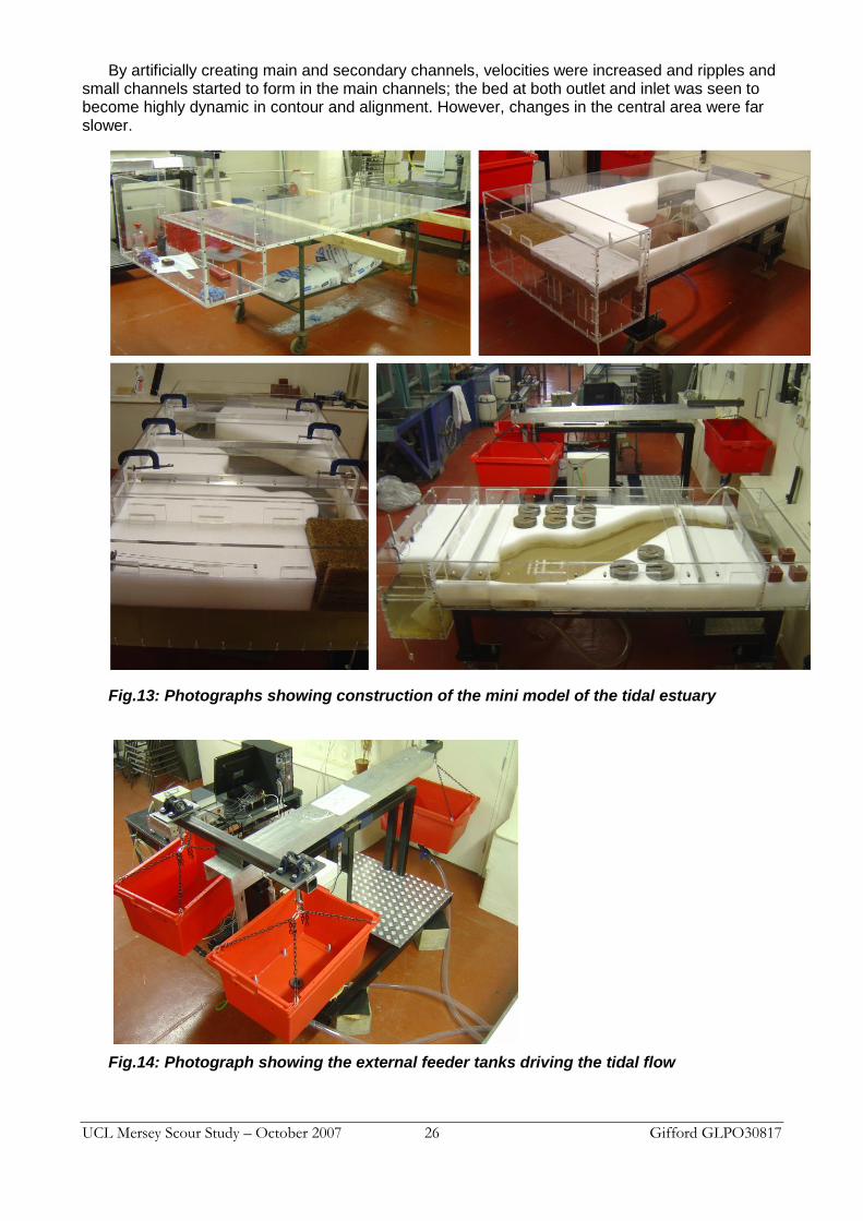
To simulate tidal flow into and out of the model, the inlet was fed by a pair of tanks and the outlet by another tank. These tanks were mounted on a vertically oscillating beam pivoted about its centre (see fig.14). Controlled by computer, the oscillation of the beam simulates the tide: during the flood phase, the water level increases in the external feeder tank at the inlet (seaward) end and water enters the model by gravity and flows upstream (inland). At the same time the tank connected to the inland end is lowered, allowing water to flow out into the external tank and be stored. The tank at the inland end is important, because when the tide comes in, the upstream reaches of the Mersey act as a reservoir, and it is necessary to maintain this characteristic in the model. During the ebb phase, the process is reversed as the tank at the inland end rises and those at the seaward end fall. The flood tide was programmed rise twice as fast as the ebb tide, creating an asymmetric flow similar to that experienced in the Upper Mersey.
Steady river flow was simulated by a pump taking the water from the seaward end of the model and transferring it to the inland end. The flow rate was insignificant compared to the tidal flows but could be increased to simulate a major storm event.
4.2 Model tuning
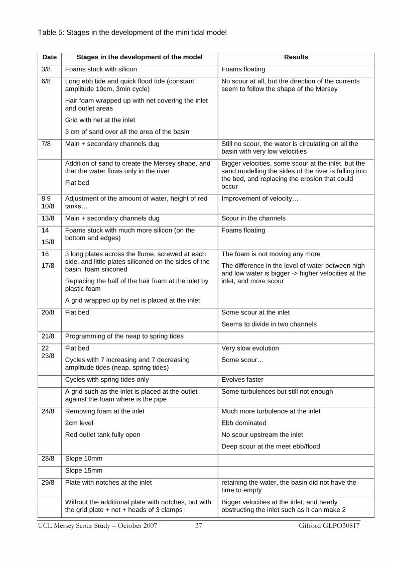
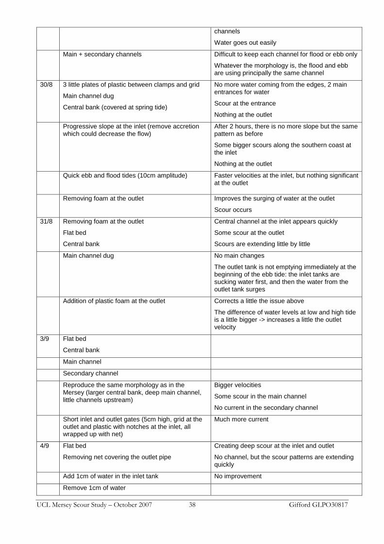
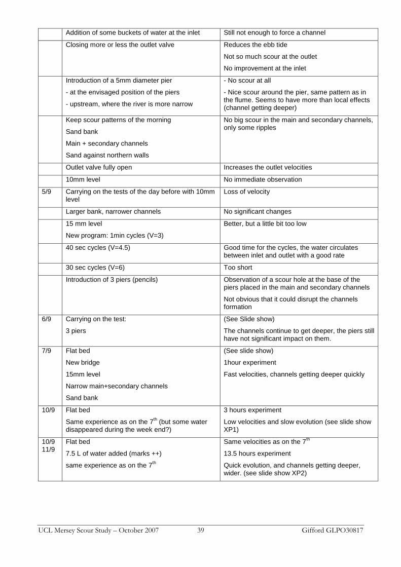
Many parameters in the model could be modified to enhance the flow rate and come closer to the conditions in the Mersey Estuary. Table 5 lists the various changes made to the inlet and outlet layouts, the slope of the basin, the height of the oscillating tanks, the amount of water, the different possibilities in the programming of the oscillations (form, speed, amplitude of the cycles), the form of the initial sand bed and so on. There were so many factors to take into account that, for reasons of time constraint, the main part of the work was spent determining the best configuration.
4.3 Results
4.3.1 Channel formation
Starting from a completely flat bed, the highest velocities were concentrated at the inlet and at the outlet of the model. The velocities decreased when the flow entered the central zone where (in the actual Mersey) there is normally a sand bank surrounded by two channels. General scour patterns appeared rapidly at both ends of the basin, and propagated towards the central zone. These bed features formed locally-deep channels and small accretions that moved along the inlet or outlet, but they were very dependant to the inlet or outlet configurations. Such features did not propagate to the central zone, even after some hours of running. We can assume that the patterns developing from both ends could join, but it would take an impractically long time for this process to lead to formation of the central sand bank which would in turn increase the velocities in the channels.
UCL Mersey Scour Study – October 2007 26 Gifford GLPO30817
By artificially creating main and secondary channels, velocities were increased and ripples and small channels started to form in the main channels; the bed at both outlet and inlet was seen to become highly dynamic in contour and alignment. However, changes in the central area were far slower.
Fig.13: Photographs showing construction of the mini model of the tidal estuary
Fig.14: Photograph showing the external feeder tanks driving the tidal flow
UCL Mersey Scour Study – October 2007 27 Gifford GLPO30817
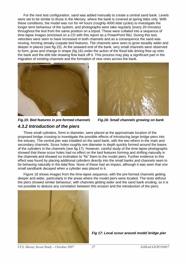
For the next test configuration, sand was added manually to create a central sand bank. Levels were set to be similar to those in the Mersey, where the bank is covered at spring tides only. With these conditions, the model was run for 44 hours (roughly 4000 tidal cycles) to investigate the longer term behaviour of the system, and photographs were take regularly (every 20 minutes) throughout the test from the same position on a tripod. These were collated into a sequence of time-lapse images (enclosed on a CD with this report as a PowerPoint file). During this test, velocities were seen to have increased in both channels and as a consequence the sand was moving, forming streaky cuspate bed features. The channels were seen to grow steadily wider and deeper in places (see fig.15). At the seaward end of the bank, very small channels were observed to form, grow and change in shape (fig.16) under the action of the flood tide driving flow up onto the bank and the ebb tide drawing flow back off it. This process may play a significant part in the migration of existing channels and the formation of new ones across the bank.
Fig.15: Bed features in pre-formed channels Fig.16: Small channels growing on bank
4.3.2 Introduction of the piers
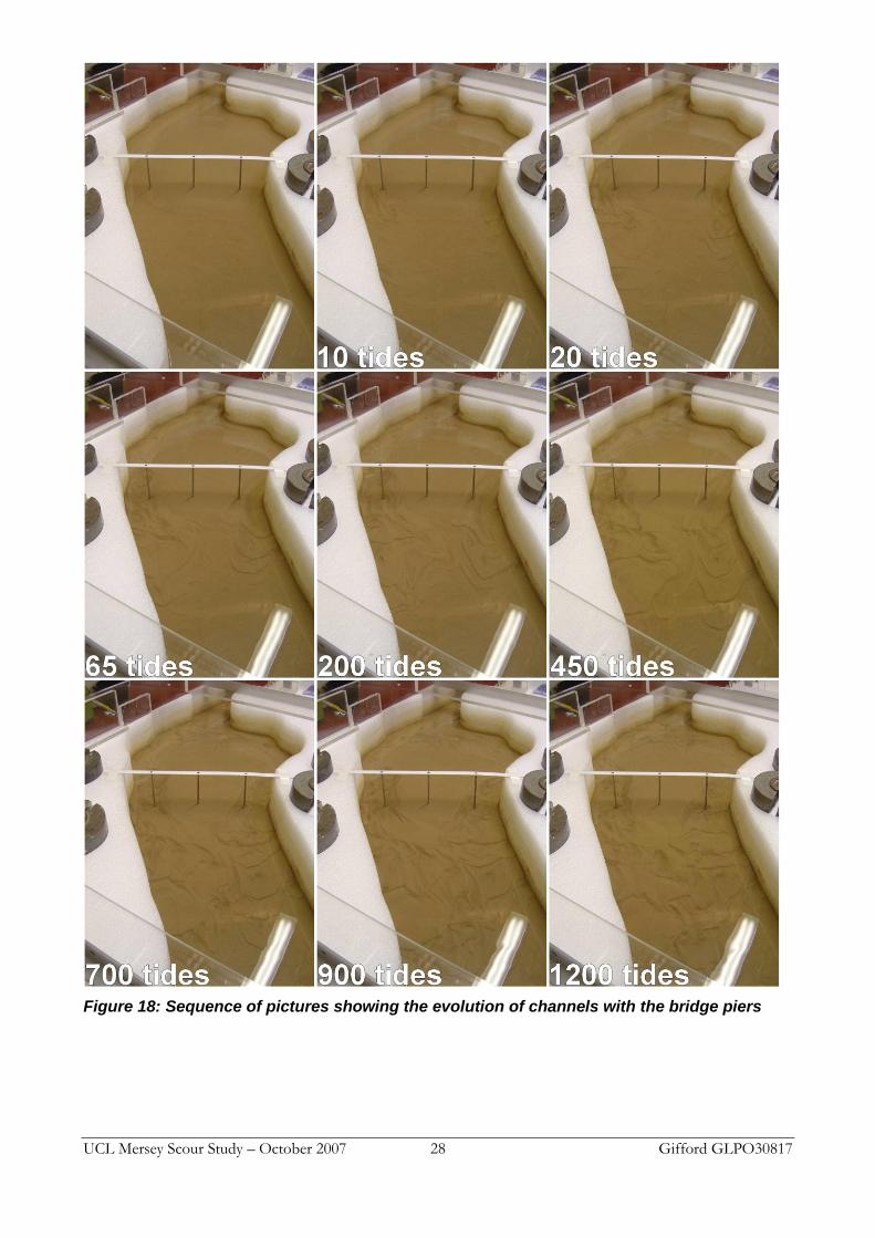
Three small cylinders, 5mm in diameter, were placed at the approximate location of the proposed bridge crossing to investigate the possible effects of introducing large bridge piers into the estuary. The central pier was installed on the sand bank, with the two others in the main and secondary channels. Scour holes roughly one diameter in depth quickly formed around the bases of the cylinders in the channels (see fig.17). However, careful study of the time-lapse photographs showed that these scour holes had no effect on the bed features forming and shifting naturally in the channels and showed no inclination to “fix” them to the model piers. Further evidence to this effect was found by placing additional cylinders directly into the small banks and channels seen to be behaving naturally in the tidal flow. None of these had an impact, although it was seen that one small sandbank decayed when a cylinder was placed in it.
Figure 18 shows images from the time-lapse sequence, with the pre-formed channels getting deeper and wider, particularly in the areas where the model piers were located. The tests without the piers showed similar behaviour, with channels getting wider and the sand bank eroding, so it is not possible to deduce any correlation between this erosion and the introduction of the piers.
Fig 17: Local scour around model bridge pier
UCL Mersey Scour Study – October 2007 28 Gifford GLPO30817
Figure 18: Sequence of pictures showing the evolution of channels with the bridge piers
UCL Mersey Scour Study – October 2007 29 Gifford GLPO30817
4.4 Conclusion
Within the times allocated to this part of the project it has not been possible to resolve all the issues identified at the outset or to develop the model sufficiently to reproduce the behaviour of the main and secondary channels in the Mersey Estuary. Nor does the model include the effects of waves, salinity, or variations in sediment size. However, it has been shown that a mini tidal model is capable of reproducing certain important aspects of natural channel evolution in a tidal estuary. The site of the proposed new crossing appears, in terms of sediment dynamics, to be relatively inactive in comparison to regions upstream and downstream. The introduction of model bridge piers had no significant impact on the natural behaviour of the bed features in the model, and there was no evidence of channel “fixing”.
Encouraged by these observations, the model is currently being used for a more generic investigation of sediment dynamics and morphology in a tidal estuary. This study will look at the effects of increasing the tidal amplitude, of using different, more mobile sediment, and of different spring-neap tidal cycles.
References and bibliography
Blench, T., 1962, Discussion of "scour at bridge crossings", by E.M. Laursen: Transactions of American Society of Civil Engineers, v. 127, pp.180-183.
Breusers, H.N.C., Nicolet, G. and Shen, H.W., 1977 Local scour around cylindrical piers, J.Hydraulic Res., IAHR, 15, 3, pp.211-252
Chitale, S.V., 1962, Scour at bridge crossings: Transactions of the American Society of Civil Engineers, v. 127, no. 1, pp.191-196.
Gibson, A.H., 1933, Construction and operation of a tidal model of the Severn Estuary. H.M.S.O.
Gifford, 2004, Case study of bridges constructed in highly mobile estuaries or river beds (B4027.TR03.04)
Gifford, 2007, Mersey Gateway: Morphological monitoring interpretative report (B4027.TR03.07)
Gifford, 2005, Additional Modelling – Mersey Gateway. Technical Note A: Residual Modelling – Stage I (R.1241a)
Gifford, 2005, Additional Modelling – Mersey Gateway. Technical Note B: Residual Modelling – Stage II (R.1241b)
Gifford, 2005, Additional Modelling – Mersey Gateway. Technical Note C: Flat Bed Morphological Modelling (R.1241c)
Hancu, S., 1971, Sur le calcul des affouillements locaux dans la zone des piles des ponts. Proc. 14th International Association of Hydraulic Research Congress: Paris, France, pp.299-313
Hoffmans, G.J.C.M. and Verheij, H.J., 1997, Scour Manual. A.A.Balkema, Rotterdam
Inglis, S.C., 1949, Maximum depth of scour at heads of guide banks and groynes, pier noses, and downstream of bridges-The behavior and control of rivers and canals: Poona, India, Indian Waterways Experimental Station, pp.327-348
Jain, S.C., 1981, Maximum clear-water scour around cylindrical piers. J.Hydraulic Engng, 107, 5, pp.611- 626.
Johnson, P.A., 1992, Reliability-based pier scour engineering. J.Hydraulic Engng, 118, 10, pp.1344-1358
Jones, J.S. and Sheppard, D.M., 2000, Scour at wide bridge piers. ASCE, US Department of Transportation, Federal Highway Administration, Turner-Fairbank Highway Res. Center, 10 pp.

UCL Mersey Scour Study – October 2007 30 Gifford GLPO30817
Laursen, E.M., 1962, Scour at bridge crossings: Transactions of the American Society of Civil Engineers, v. 127, part 1, pp.166-209.
Laursen, E.M. and Toch, A., 1956, Scour around bridge piers and abutments, Bulletin 4, Iowa Highway Research Board, State University of Iowa, 60pp.
Mann, K. and Stevenson, T.A., 1995, The use of mini tidal hydraulic models of estuaries. HR Wallingford Report SR395
May, R.W.P. and Willoughby, I.R., 1990, Local scour around large obstructions. HR Wallinford Report SR 240
May R.W.P. & Escarameia M., 2002, Local scour around structures in tidal flows. Proc.1st Int.Conf on Scour of Foundations, Texas A&M University, pp.320-331
May, R.W.P., Ackers, J.C. and Kirby, A.M., 2002, Manual on scour at bridges and other hydraulic structures. Construction Industry Research and Information Association.
Melville, B.W. and Sutherland, A.J., 1988, Design methods for local scour at bridge piers. J.Hydraulic Engng, 114, 10, pp.1210-1226
Morten Sand Jensen et al., 2006, Offshore Wind Turbine situated in Areas with Strong Currents, Offshore Center Denmark
Qadar, A., 1981, The vortex scour mechanism at bridge piers. Proc.ICE, 71, Pt.2.
Reynolds, O., 1887, On certain laws relating to the regime of rivers and estuaries and on the possibility of experiments on a small scale. Brit. Assoc. Rept. 867, pp.555-562
Richardson, E.V., and Davis, S.R., 2001, Evaluating scour at bridges (4th ed.): Washington, DC, Federal Highway Administration Hydraulic Engineering Circular No. 18, FHWA NHI 01-001, 378 p.
Shen, H.W., Schneider, V.R., and Karaki, S., 1969, Local scour around bridge piers: J.Hydraulic Engng, 95, HY6, pp.1919-1940.
Sheppard, D.M., 2003, Large scale and live bed local pier scour experiments, phase 2, live bed experiments. Final report, University of Florida.
Simons, R.R., Weller, J. and Whitehouse, R.J.S., 2007, Scour development around truncated cylindrical structures. Proc. Coastal Structures Conf, Venice, July 2007
Sumer, B.M., Christiansen, N. and Fredsoe, J., 1993, Influence of cross section on wave scour around piles. J.Waterway, Port, Coastal and Ocean Engng, ASCE, 119, 5, 477-495
Vernon-Harcourt, L.F., 1890, Effects of training walls in an estuary. Royal Society of London, 30 January, 1890
Whitehouse R., 1998, Scour at Marine Structures. Thomas Telford, London, 216pp.
http://radio.weblogs.com/0100021/stories/2002/03/06/sedimentTransportInAnridun.html
http://www.fhwa.dot.gov/engineering/hydraulics/pubs/03052/05.cfm

UCL Mersey Scour Study – October 2007 31 Gifford GLPO30817
Tables
UCL Mersey Scour Study – October 2007 32 Gifford GLPO30817
Table 1: Formulae predicting the maximum scour depth at the equilibrium
Author Formula Eq.
Sheppard (2003)
For clear-water scour:
(1)
(1a)
(1b)
(1c)
May, Ackers & Kirby (2002)
: factor of safety (the value of 1.6 corresponds to the maximum depths observed in laboratory studies).
: value based on the effect of the shape of the structure on the extent of local scour (equals 1 for a cylindrical pier).
: value based on the effect of the relative water depth on the depth of local scour. It can be calculated using equations 2a and 2b from May and Willoughby (1990):
: factor quantifying the effect of the flow velocity on the scour depth which can be determined using equations 2c, d and e from May, Ackers & Kirby (2002):
: factor which quantifies the effect of the alignment of the structure on the extent of scour (equals 1 for a cylindrical pier).
(2)
(2a)
(2b)
(2c)
(2d)
(2e)
May & Escarameia (2002)
(3)
Richardson & Davis “CSU/HEC-18” (2001)
(4)
UCL Mersey Scour Study – October 2007 33 Gifford GLPO30817
Jones & Sheppard (2000)
For clear-water scour:
(5)
(5a)
(5b)
Richard May (1998)
(6)
Sumer et Al. (1992)
(7)
Breusers & Al (1977)
equals 1.5 but shall be taken as 2.0 in design.
depends on the ratio between the average current velocity and the critical velocity as:
is a shape factor (equals 1for a circular pile).
depends on the angle of attack and is 1.0 for a circular pile.
(8)
(8a)
(8b)
(8c)
Hancu (1971)
(9)
Shen Maza (1969)
(10a)
(10b)
Shen et al. (1969)
(11)
Laursen (1963)
(12)
Chitale (1962)
(13)
Laursen & Toch (1956)
(14)

UCL Mersey Scour Study – October 2007 34 Gifford GLPO30817
Table 2: Experiments run in the flume
E
quili
brium
reach
ed
Ye
s
Ye
s
No
No
Ye
s
Ye
s
No
Ye
s
Ye
s
Ye
s
Ru
nn
ing
hou
rs
8 h
ou
rs
19 h
ou
rs
4.5
hours
8.5
hours
44 h
ou
rs
26 h
ou
rs
22 h
ou
rs
28 h
ou
rs
18.5
hou
rs
34 h
ou
rs
Ma
xim
um
sco
ur
depth
15 m
m
22 m
m
93 m
m
93 m
m
77 m
m
57 m
m
54 t
o 7
1 m
m
39 m
m
31 t
o 3
8 m
m
45 m
m
Oth
er
para
mete
rs
Dis
rupte
d e
vo
lutio
n
Re
vers
e c
urr
ent
Dis
rupte
d e
volu
tio
n
Cle
an
sa
nd
Re
vers
e c
urr
ent
Cle
an
sa
nd
Sco
ur
typ
e
No
sco
ur
No
sco
ur
Liv
e-
bed
sco
ur
Liv
e-b
ed
sco
ur
Cle
ar-
wa
ter
sco
ur
Cle
ar-
wa
ter
sco
ur
Cle
ar-
wa
ter
sco
ur
Cle
ar-
wa
ter
sco
ur
Cle
ar-
wa
ter
sco
ur
Cle
ar-
wa
ter
sco
ur
Ve
locity
11.4
cm
/se
c
10.8
cm
/se
c
25 c
m/s
ec
21 c
m/s
ec
16.9
cm
/se
c
17 c
m/s
ec
17.2
cm
/se
c
17.5
cm
/se
c
16.7
cm
/se
c
15 c
m/s
ec
Wa
ter
dep
th
80 m
m
100
mm
75 m
m
75 m
m
75 m
m
50 m
m
50 m
m
50 m
m
50 m
m
50 m
m
XP
1
2
3
4
5
6
7
8
9
10
UCL Mersey Scour Study – October 2007 35 Gifford GLPO30817
Table 3: Equivalences between the flume-scale and real scale:
Full-scale values Small-scale values
Cylinder diameter 10 m 150 mm
Very high water depth (1in200 year event) 7 m 105 mm
High tide water depth 5 m 75 mm
Medium water depth 3.3 m 50 mm
Maximum velocity 2 m/sec 24.4 cm/sec
Cycle half-period 6 hours 45 min
UCL Mersey Scour Study – October 2007 36 Gifford GLPO30817
Table 4: Comparison between predicted scour depth and experimental flume-scale observations:
Case studies: 1 2 3 4 5 6 7 8 9 10
Water depth h: (m) 0.08 0.1 0.075 0.075 0.075 0.05 0.05 0.05
mean U: (m/s) 0.114 0.108 0.25 0.21 0.169 0.17 0.175 0.15
Sand diameter: (mm) 15 15 15 15 15 15 15 15
cylinder diameter D: (m) 0.15 0.15 0.15 0.15 0.15 0.15 0.15 0.15
Froude No.: 0.13 0.11 0.29 0.24 0.2 0.24 0.25 0.21
Critical velocity: (m/s) 0.22 0.22 0.21 0.21 0.21 0.2 0.2 0.2
Observed maximum scour (m) 0.015 0.022 0.093 0.093 0.077 0.057 0.039 0.045
Observed max scour: S/D 0.10 0.15 0.62 0.62 0.51 0.38 0.26 0.30
Predicted max scour: S/D
Laursen & Toch (1956) 1.24 1.32 1.22 1.22 1.22 1.08 1.08 1.08
Laursen (1963) 0.98 1.09 0.95 0.95 0.95 0.77 0.77 0.77
Shen et al. (1969) 1.09 1.12 1.08 1.08 1.08 1.03 1.03 1.03
Hancu (1971) 0.76 0.79 0.76 0.76 0.76 0.72 0.72 0.72
Breusers & al (1977) K=2.0 0.05 0.00 0.92 0.89 0.54 0.45 0.48 0.32
Qadar (1981) 2.63 2.63 2.63 2.63 2.63 2.63 2.63 2.63
Jain (1981) 1.07 1.12 1.06 1.06 1.06 1.00 1.00 1.00
Sumer et al. (1992) 1.30 1.30 1.30 1.30 1.30 1.30 1.30 1.30
May, Ackers & Kirby (2002) 0.15 0.12 0.58 0.57 0.39 0.35 0.37 0.27
Richardson & Davis (2001) 0.73 0.74 1.01 0.94 0.86 0.81 0.82 0.77
Richard May (1998) 0.07 0.00 1.02 0.75 0.46 0.37 0.39 0.27
May & Escarameia (2002) 0.02 0.00 0.79 0.66 0.51 0.44 0.46 0.35
Jones & Sheppard (2000) 0.20 0.13 1.17 0.89 0.59 0.61 0.64 0.47
Sheppard (2003) 0.29 0.07 0.96 1.00 0.91 0.85 0.86 0.76
Chitale (1962) 0.14 0.10 0.48 0.39 0.29 0.26 0.27 0.22
Shen Maza (1969) 0.10 0.09 0.59 0.52 0.21 0.45 0.46 0.42
Inglis (1949) 0.35 0.30 0.79 0.67 0.55 0.52 0.53 0.47
Blench (1962): Blench-Inglis II 0.50 0.46 0.98 0.86 0.72 0.67 0.68 0.70
UCL Mersey Scour Study – October 2007 37 Gifford GLPO30817
Table 5: Stages in the development of the mini tidal model
Date Stages in the development of the model Results
3/8 Foams stuck with silicon Foams floating
6/8 Long ebb tide and quick flood tide (constant amplitude 10cm, 3min cycle)
Hair foam wrapped up with net covering the inlet and outlet areas
Grid with net at the inlet
3 cm of sand over all the area of the basin
No scour at all, but the direction of the currents seem to follow the shape of the Mersey
7/8 Main + secondary channels dug Still no scour, the water is circulating on all the basin with very low velocities
Addition of sand to create the Mersey shape, and that the water flows only in the river
Flat bed
Bigger velocities, some scour at the inlet, but the sand modelling the sides of the river is falling into the bed, and replacing the erosion that could occur
8 9 10/8
Adjustment of the amount of water, height of red tanks…
Improvement of velocity…
13/8 Main + secondary channels dug Scour in the channels
14
15/8
Foams stuck with much more silicon (on the bottom and edges)
Foams floating
16
17/8
3 long plates across the flume, screwed at each side, and little plates siliconed on the sides of the basin, foam siliconed
Replacing the half of the hair foam at the inlet by plastic foam
A grid wrapped up by net is placed at the inlet
The foam is not moving any more
The difference in the level of water between high and low water is bigger -> higher velocities at the inlet, and more scour
20/8 Flat bed Some scour at the inlet
Seems to divide in two channels
21/8 Programming of the neap to spring tides
22 23/8
Flat bed
Cycles with 7 increasing and 7 decreasing amplitude tides (neap, spring tides)
Very slow evolution
Some scour…
Cycles with spring tides only Evolves faster
A grid such as the inlet is placed at the outlet against the foam where is the pipe
Some turbulences but still not enough
24/8 Removing foam at the inlet
2cm level
Red outlet tank fully open
Much more turbulence at the inlet
Ebb dominated
No scour upstream the inlet
Deep scour at the meet ebb/flood
28/8 Slope 10mm
Slope 15mm
29/8 Plate with notches at the inlet retaining the water, the basin did not have the time to empty
Without the additional plate with notches, but with the grid plate + net + heads of 3 clamps
Bigger velocities at the inlet, and nearly obstructing the inlet such as it can make 2
UCL Mersey Scour Study – October 2007 38 Gifford GLPO30817
channels
Water goes out easily
Main + secondary channels Difficult to keep each channel for flood or ebb only
Whatever the morphology is, the flood and ebb are using principally the same channel
30/8 3 little plates of plastic between clamps and grid
Main channel dug
Central bank (covered at spring tide)
No more water coming from the edges, 2 main entrances for water
Scour at the entrance
Nothing at the outlet
Progressive slope at the inlet (remove accretion which could decrease the flow)
After 2 hours, there is no more slope but the same pattern as before
Some bigger scours along the southern coast at the inlet
Nothing at the outlet
Quick ebb and flood tides (10cm amplitude) Faster velocities at the inlet, but nothing significant at the outlet
Removing foam at the outlet Improves the surging of water at the outlet
Scour occurs
31/8 Removing foam at the outlet
Flat bed
Central bank
Central channel at the inlet appears quickly
Some scour at the outlet
Scours are extending little by little
Main channel dug No main changes
The outlet tank is not emptying immediately at the beginning of the ebb tide: the inlet tanks are sucking water first, and then the water from the outlet tank surges
Addition of plastic foam at the outlet Corrects a little the issue above
The difference of water levels at low and high tide is a little bigger -> increases a little the outlet velocity
3/9 Flat bed
Central bank
Main channel
Secondary channel
Reproduce the same morphology as in the Mersey (larger central bank, deep main channel, little channels upstream)
Bigger velocities
Some scour in the main channel
No current in the secondary channel
Short inlet and outlet gates (5cm high, grid at the outlet and plastic with notches at the inlet, all wrapped up with net)
Much more current
4/9 Flat bed
Removing net covering the outlet pipe
Creating deep scour at the inlet and outlet
No channel, but the scour patterns are extending quickly
Add 1cm of water in the inlet tank No improvement
Remove 1cm of water
UCL Mersey Scour Study – October 2007 39 Gifford GLPO30817
Addition of some buckets of water at the inlet Still not enough to force a channel
Closing more or less the outlet valve Reduces the ebb tide
Not so much scour at the outlet
No improvement at the inlet
Introduction of a 5mm diameter pier
- at the envisaged position of the piers
- upstream, where the river is more narrow
- No scour at all
- Nice scour around the pier, same pattern as in the flume. Seems to have more than local effects (channel getting deeper)
Keep scour patterns of the morning
Sand bank
Main + secondary channels
Sand against northern walls
No big scour in the main and secondary channels, only some ripples
Outlet valve fully open Increases the outlet velocities
10mm level No immediate observation
5/9 Carrying on the tests of the day before with 10mm level
Loss of velocity
Larger bank, narrower channels No significant changes
15 mm level
New program: 1min cycles (V=3)
Better, but a little bit too low
40 sec cycles (V=4.5) Good time for the cycles, the water circulates between inlet and outlet with a good rate
30 sec cycles (V=6) Too short
Introduction of 3 piers (pencils) Observation of a scour hole at the base of the piers placed in the main and secondary channels
Not obvious that it could disrupt the channels formation
6/9 Carrying on the test:
3 piers
(See Slide show)
The channels continue to get deeper, the piers still have not significant impact on them.
7/9 Flat bed
New bridge
15mm level
Narrow main+secondary channels
Sand bank
(See slide show)
1hour experiment
Fast velocities, channels getting deeper quickly
10/9 Flat bed
Same experience as on the 7th (but some water
disappeared during the week end?)
3 hours experiment
Low velocities and slow evolution (see slide show XP1)
10/9 11/9
Flat bed
7.5 L of water added (marks ++)
same experience as on the 7th
Same velocities as on the 7th
13.5 hours experiment
Quick evolution, and channels getting deeper, wider. (see slide show XP2)

UCL Mersey Scour Study – October 2007 40 Gifford GLPO30817
Results from flume experiments:
EXPERIMENT 1
Water depth: 80mm
Average velocity: 11.4 cm/sec
Maximum scour depth: 15 mm
Time (hours) Depth (mm) Time (hours)
Depth (mm) Time (hours)
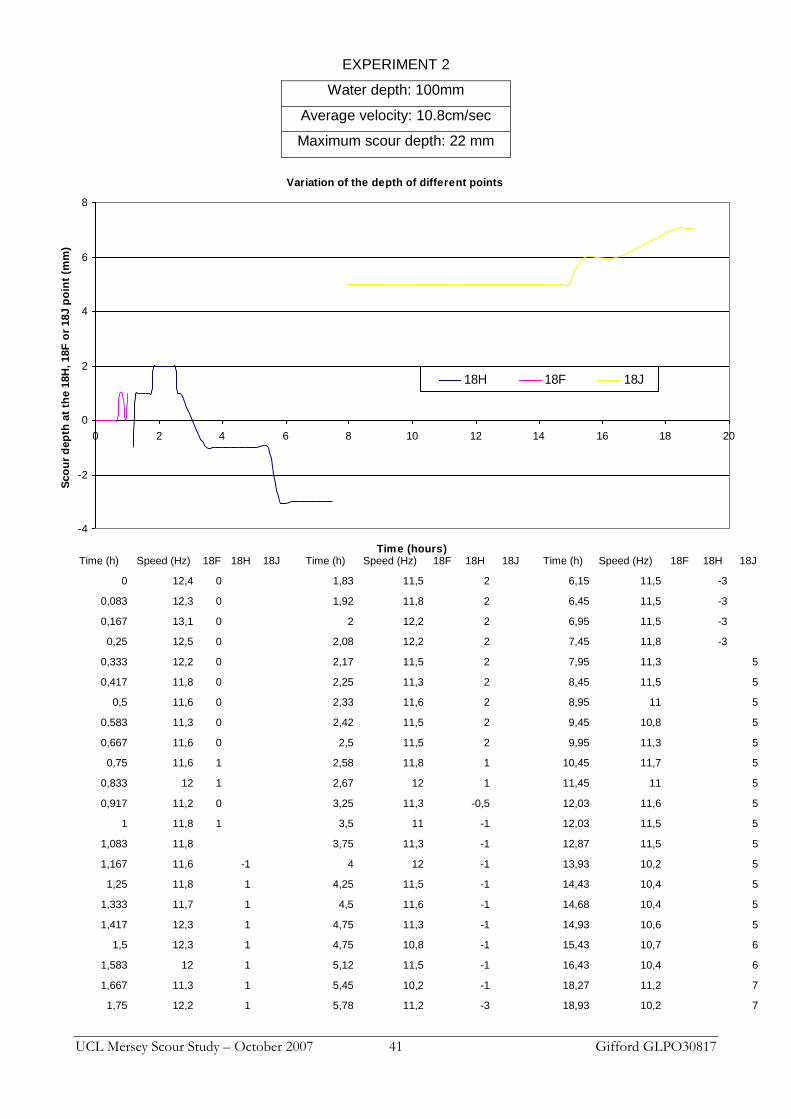
UCL Mersey Scour Study – October 2007 41 Gifford GLPO30817
Variation of the depth of different points
-4
-2
0
2
4
6
8
0 2 4 6 8 10 12 14 16 18 20
Time (hours)
Sco
ur
dep
th a
t th
e 1
8H
, 18F
or
18J p
oin
t (m
m)
18H 18F 18J
EXPERIMENT 2
Water depth: 100mm
Average velocity: 10.8cm/sec
Maximum scour depth: 22 mm
Time (h) Speed (Hz) 18F 18H 18J Time (h) Speed (Hz) 18F 18H 18J Time (h) Speed (Hz) 18F 18H 18J
0 12,4 0 1,83 11,5 2 6,15 11,5 -3
0,083 12,3 0 1,92 11,8 2 6,45 11,5 -3
0,167 13,1 0 2 12,2 2 6,95 11,5 -3
0,25 12,5 0 2,08 12,2 2 7,45 11,8 -3
0,333 12,2 0 2,17 11,5 2 7,95 11,3 5
0,417 11,8 0 2,25 11,3 2 8,45 11,5 5
0,5 11,6 0 2,33 11,6 2 8,95 11 5
0,583 11,3 0 2,42 11,5 2 9,45 10,8 5
0,667 11,6 0 2,5 11,5 2 9,95 11,3 5
0,75 11,6 1 2,58 11,8 1 10,45 11,7 5
0,833 12 1 2,67 12 1 11,45 11 5
0,917 11,2 0 3,25 11,3 -0,5 12,03 11,6 5
1 11,8 1 3,5 11 -1 12,03 11,5 5
1,083 11,8 3,75 11,3 -1 12,87 11,5 5
1,167 11,6 -1 4 12 -1 13,93 10,2 5
1,25 11,8 1 4,25 11,5 -1 14,43 10,4 5
1,333 11,7 1 4,5 11,6 -1 14,68 10,4 5
1,417 12,3 1 4,75 11,3 -1 14,93 10,6 5
1,5 12,3 1 4,75 10,8 -1 15,43 10,7 6
1,583 12 1 5,12 11,5 -1 16,43 10,4 6
1,667 11,3 1 5,45 10,2 -1 18,27 11,2 7
1,75 12,2 1 5,78 11,2 -3 18,93 10,2 7
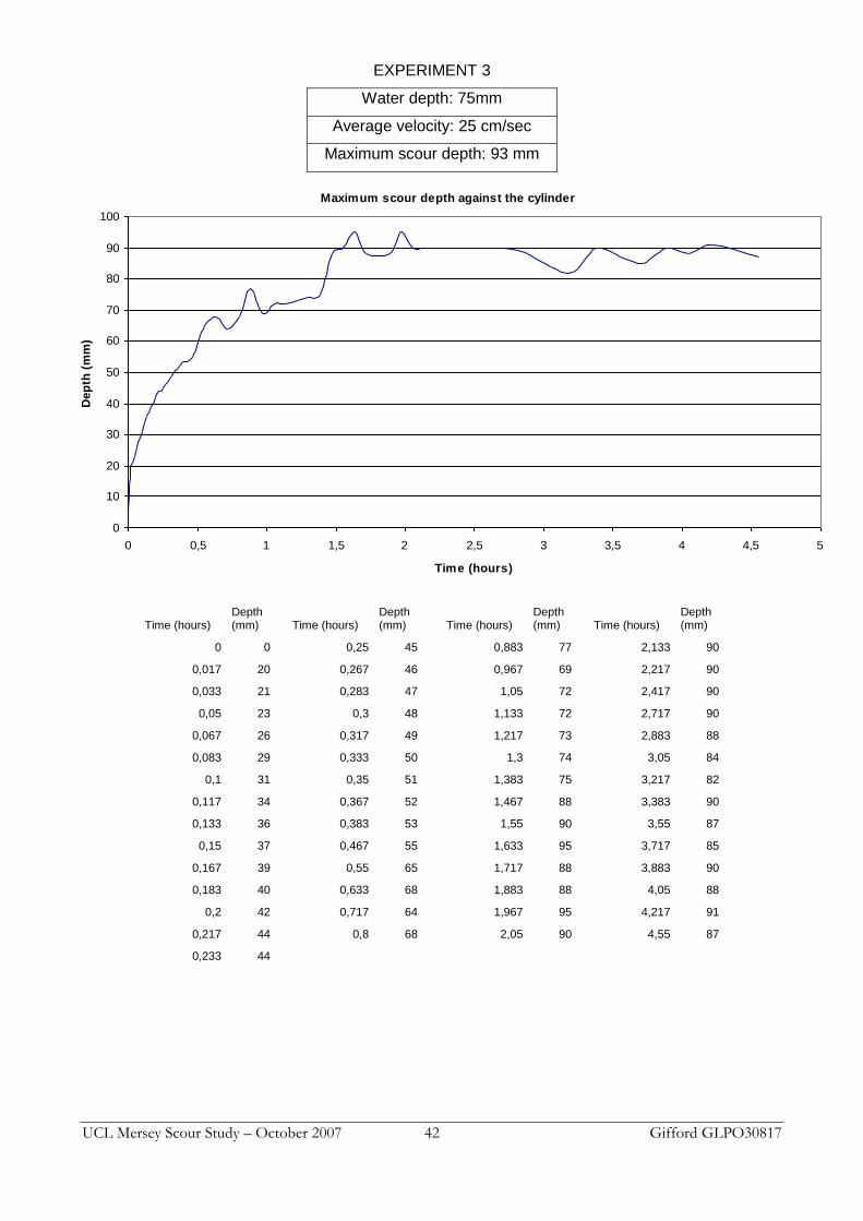
UCL Mersey Scour Study – October 2007 42 Gifford GLPO30817
Maximum scour depth against the cylinder
0
10
20
30
40
50
60
70
80
90
100
0 0,5 1 1,5 2 2,5 3 3,5 4 4,5 5
Time (hours)
Dep
th (
mm
)EXPERIMENT 3
Water depth: 75mm
Average velocity: 25 cm/sec
Maximum scour depth: 93 mm
Time (hours) Depth (mm) Time (hours)
Depth (mm) Time (hours)
Depth (mm) Time (hours)
Depth (mm)
0 0 0,25 45 0,883 77 2,133 90
0,017 20 0,267 46 0,967 69 2,217 90
0,033 21 0,283 47 1,05 72 2,417 90
0,05 23 0,3 48 1,133 72 2,717 90
0,067 26 0,317 49 1,217 73 2,883 88
0,083 29 0,333 50 1,3 74 3,05 84
0,1 31 0,35 51 1,383 75 3,217 82
0,117 34 0,367 52 1,467 88 3,383 90
0,133 36 0,383 53 1,55 90 3,55 87
0,15 37 0,467 55 1,633 95 3,717 85
0,167 39 0,55 65 1,717 88 3,883 90
0,183 40 0,633 68 1,883 88 4,05 88
0,2 42 0,717 64 1,967 95 4,217 91
0,217 44 0,8 68 2,05 90 4,55 87
0,233 44
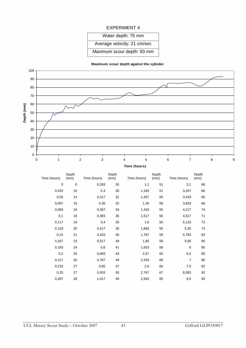
UCL Mersey Scour Study – October 2007 43 Gifford GLPO30817
Maximum scour depth against the cylinder
0
10
20
30
40
50
60
70
80
90
100
0 1 2 3 4 5 6 7 8 9
Time (hours)
Dep
th (
mm
)
EXPERIMENT 4
Water depth: 75 mm
Average velocity: 21 cm/sec
Maximum scour depth: 93 mm
Time (hours) Depth (mm) Time (hours)
Depth (mm) Time (hours)
Depth (mm) Time (hours)
Depth (mm)
0 0 0,283 30 1,1 51 3,1 66
0,033 10 0,3 30 1,183 51 3,267 66
0,05 14 0,317 31 1,267 55 3,433 66
0,067 15 0,35 32 1,35 58 3,833 68
0,083 16 0,367 34 1,433 55 4,217 74
0,1 18 0,383 35 1,517 56 4,517 71
0,117 19 0,4 35 1,6 56 5,133 72
0,133 20 0,417 35 1,683 55 5,35 74
0,15 21 0,433 36 1,767 59 5,783 83
0,167 23 0,517 39 1,85 58 5,95 80
0,183 24 0,6 41 1,933 58 6 85
0,2 25 0,683 43 2,67 65 6,5 85
0,217 26 0,767 49 2,433 68 7 86
0,233 27 0,85 47 2,6 66 7,5 82
0,25 27 0,933 50 2,767 67 8,083 92
0,267 28 1,017 49 2,933 65 8,5 93
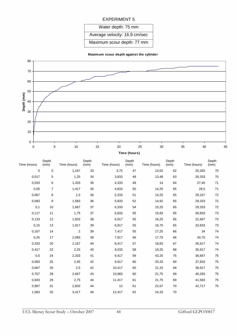
UCL Mersey Scour Study – October 2007 44 Gifford GLPO30817
Maximum scour depth against the cylinder
0
10
20
30
40
50
60
70
80
0 5 10 15 20 25 30 35 40 45
Time (hours)
Dep
th (
mm
)EXPERIMENT 5
Water depth: 75 mm
Average velocity: 16.9 cm/sec
Maximum scour depth: 77 mm
Time (hours) Depth (mm) Time (hours)
Depth (mm) Time (hours)
Depth (mm) Time (hours)
Depth (mm) Time (hours)
Depth (mm)
0 0 1,167 33 3,75 47 13,02 62 25,283 70
0,017 5 1,25 34 3,833 48 13,48 63 26,333 70
0,033 6 1,333 35 4,333 49 14 64 27,45 71
0,05 7 1,417 35 4,833 50 14,25 65 28,5 71
0,067 8 1,5 36 5,333 51 14,25 65 29,167 72
0,083 9 1,583 36 5,833 52 14,92 65 29,333 72
0,1 10 1,667 37 6,333 54 15,25 65 29,333 72
0,117 11 1,75 37 6,833 55 15,83 65 30,833 73
0,133 12 1,833 38 6,917 55 16,25 65 31,667 73
0,15 13 1,917 39 6,917 55 16,75 65 32,833 73
0,167 14 2 39 7,417 55 17,25 66 34 74
0,25 17 2,083 39 7,917 56 17,75 66 34,75 74
0,333 20 2,167 40 8,417 57 18,83 67 35,917 74
0,417 22 2,25 40 9,033 58 19,25 68 35,917 74
0,5 24 2,333 41 9,417 59 43,25 75 36,667 75
0,583 25 2,45 42 9,917 60 20,33 69 37,833 75
0,667 26 2,5 42 10,417 60 21,33 69 38,917 75
0,767 28 2,667 43 10,983 60 21,75 69 40,283 75
0,833 29 2,75 44 11,417 61 21,75 69 41,583 75
0,967 31 2,833 44 12 61 22,67 70 42,717 75
1,083 32 3,417 46 12,417 62 24,33 70
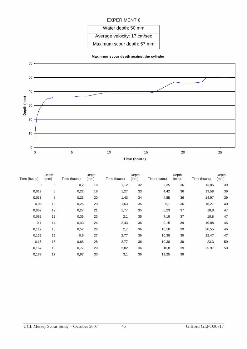
UCL Mersey Scour Study – October 2007 45 Gifford GLPO30817
Maximum scour depth against the cylinder
0
10
20
30
40
50
60
0 5 10 15 20 25
Time (hours)
Dep
th (
mm
)EXPERIMENT 6
Water depth: 50 mm
Average velocity: 17 cm/sec
Maximum scour depth: 57 mm
Time (hours) Depth (mm) Time (hours)
Depth (mm) Time (hours)
Depth (mm) Time (hours)
Depth (mm) Time (hours)
Depth (mm)
0 0 0,2 18 1,12 32 3,35 36 13,05 39
0,017 5 0,22 19 1,27 33 4,42 36 13,58 39
0,033 8 0,23 20 1,43 34 4,85 36 14,97 39
0,05 10 0,25 20 1,63 35 5,1 36 16,27 40
0,067 12 0,27 21 1,77 35 6,23 37 18,8 47
0,083 13 0,35 23 2,1 35 7,18 37 18,8 47
0,1 14 0,43 24 2,43 36 9,15 39 19,88 46
0,117 15 0,52 26 2,7 36 10,18 39 20,55 46
0,133 15 0,6 27 2,77 36 10,38 39 22,47 47
0,15 16 0,68 28 2,77 36 10,38 39 23,3 50
0,167 16 0,77 29 2,82 36 10,8 39 25.97 50
0,183 17 0,97 30 3,1 36 12,25 39
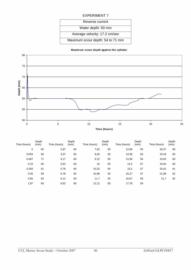
UCL Mersey Scour Study – October 2007 46 Gifford GLPO30817
Maximum scour depth against the cylinder
50
55
60
65
70
75
80
0 5 10 15 20 25
Time (hours)
Dep
th (
mm
)EXPERIMENT 7
Reverse current
Water depth: 50 mm
Average velocity: 17.2 cm/sec
Maximum scour depth: 54 to 71 mm
Time (hours) Depth (mm) Time (hours)
Depth (mm) Time (hours)
Depth (mm) Time (hours)
Depth (mm) Time (hours)
Depth (mm)
0 60 2,87 60 7,62 59 12,68 55 18,27 60
0,033 60 3,37 60 8,45 55 13,38 56 19,18 60
0,067 71 4,17 60 9,12 55 13,38 56 19,63 60
0,15 65 5,62 60 10 55 14,3 57 19,63 60
0,283 61 5,78 60 10,32 54 15,2 57 20,42 61
0,45 59 5,78 60 10,98 54 16,27 57 21,08 62
0,95 60 6,12 60 11,7 55 16,67 58 21,7 62
1,87 60 6,62 60 12,12 55 17,78 59
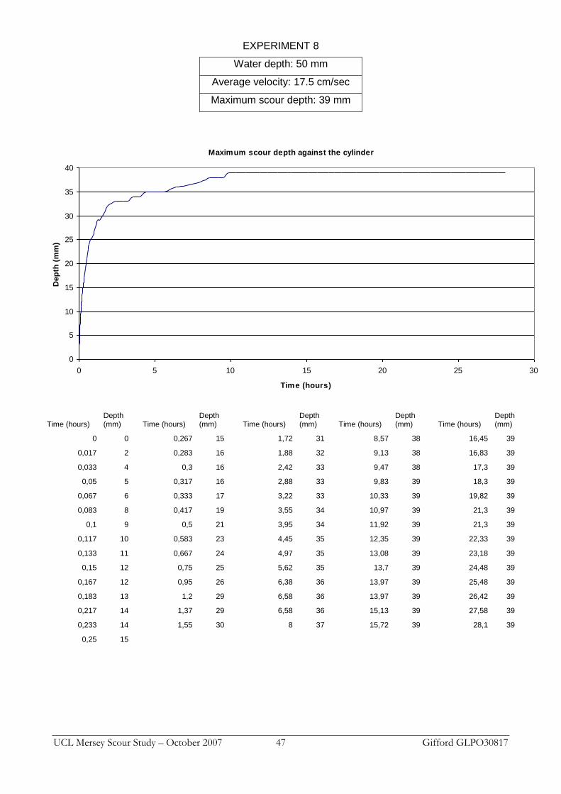
UCL Mersey Scour Study – October 2007 47 Gifford GLPO30817
Maximum scour depth against the cylinder
0
5
10
15
20
25
30
35
40
0 5 10 15 20 25 30
Time (hours)
Dep
th (
mm
)EXPERIMENT 8
Water depth: 50 mm
Average velocity: 17.5 cm/sec
Maximum scour depth: 39 mm
Time (hours) Depth (mm) Time (hours)
Depth (mm) Time (hours)
Depth (mm) Time (hours)
Depth (mm) Time (hours)
Depth (mm)
0 0 0,267 15 1,72 31 8,57 38 16,45 39
0,017 2 0,283 16 1,88 32 9,13 38 16,83 39
0,033 4 0,3 16 2,42 33 9,47 38 17,3 39
0,05 5 0,317 16 2,88 33 9,83 39 18,3 39
0,067 6 0,333 17 3,22 33 10,33 39 19,82 39
0,083 8 0,417 19 3,55 34 10,97 39 21,3 39
0,1 9 0,5 21 3,95 34 11,92 39 21,3 39
0,117 10 0,583 23 4,45 35 12,35 39 22,33 39
0,133 11 0,667 24 4,97 35 13,08 39 23,18 39
0,15 12 0,75 25 5,62 35 13,7 39 24,48 39
0,167 12 0,95 26 6,38 36 13,97 39 25,48 39
0,183 13 1,2 29 6,58 36 13,97 39 26,42 39
0,217 14 1,37 29 6,58 36 15,13 39 27,58 39
0,233 14 1,55 30 8 37 15,72 39 28,1 39
0,25 15
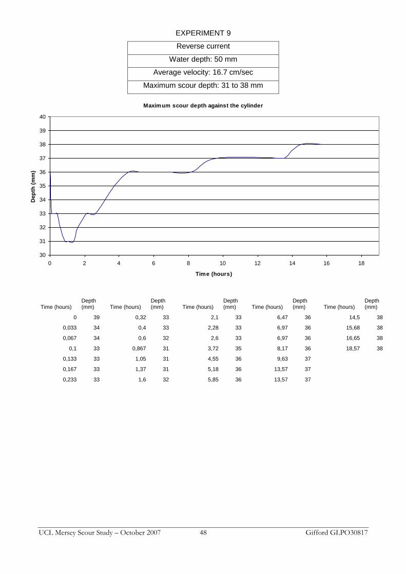
UCL Mersey Scour Study – October 2007 48 Gifford GLPO30817
Maximum scour depth against the cylinder
30
31
32
33
34
35
36
37
38
39
40
0 2 4 6 8 10 12 14 16 18
Time (hours)
Dep
th (
mm
)EXPERIMENT 9
Reverse current
Water depth: 50 mm
Average velocity: 16.7 cm/sec
Maximum scour depth: 31 to 38 mm
Time (hours) Depth (mm) Time (hours)
Depth (mm) Time (hours)
Depth (mm) Time (hours)
Depth (mm) Time (hours)
Depth (mm)
0 39 0,32 33 2,1 33 6,47 36 14,5 38
0,033 34 0,4 33 2,28 33 6,97 36 15,68 38
0,067 34 0,6 32 2,6 33 6,97 36 16,65 38
0,1 33 0,867 31 3,72 35 8,17 36 18,57 38
0,133 33 1,05 31 4,55 36 9,63 37
0,167 33 1,37 31 5,18 36 13,57 37
0,233 33 1,6 32 5,85 36 13,57 37
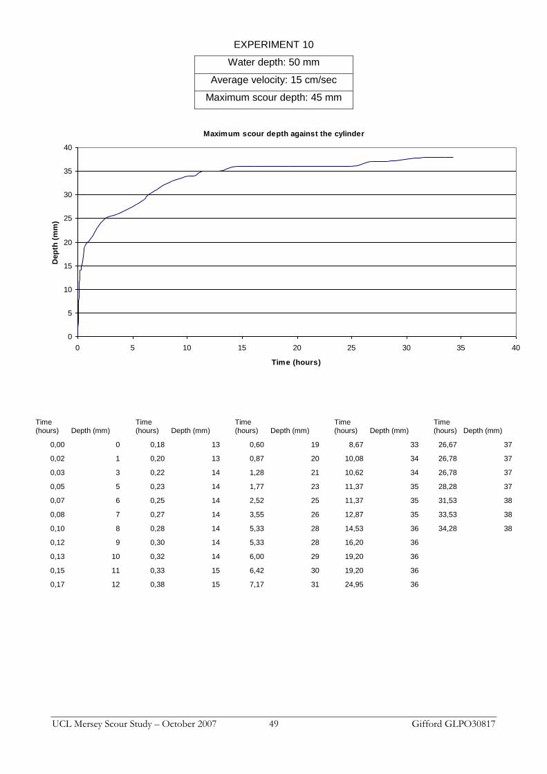
UCL Mersey Scour Study – October 2007 49 Gifford GLPO30817
Maximum scour depth against the cylinder
0
5
10
15
20
25
30
35
40
0 5 10 15 20 25 30 35 40
Time (hours)
Dep
th (
mm
)
EXPERIMENT 10
Water depth: 50 mm
Average velocity: 15 cm/sec
Maximum scour depth: 45 mm
Time (hours) Depth (mm)
Time (hours) Depth (mm)
Time (hours) Depth (mm)
Time (hours) Depth (mm)
Time (hours) Depth (mm)
0,00 0 0,18 13 0,60 19 8,67 33 26,67 37
0,02 1 0,20 13 0,87 20 10,08 34 26,78 37
0,03 3 0,22 14 1,28 21 10,62 34 26,78 37
0,05 5 0,23 14 1,77 23 11,37 35 28,28 37
0,07 6 0,25 14 2,52 25 11,37 35 31,53 38
0,08 7 0,27 14 3,55 26 12,87 35 33,53 38
0,10 8 0,28 14 5,33 28 14,53 36 34,28 38
0,12 9 0,30 14 5,33 28 16,20 36
0,13 10 0,32 14 6,00 29 19,20 36
0,15 11 0,33 15 6,42 30 19,20 36
0,17 12 0,38 15 7,17 31 24,95 36