Numerical scour modeling around parallel spur dikes in ... · 1 Numerical scour modeling around...

1

Numerical scour modeling around parallel spur dikes in FLOW-3D

Hanif Pourshahbaz1, Saeed Abbasi1, Poorya Taghvaei2

1. Department of Civil Engineering, University of Zanjan, Zanjan, Iran

2. Department of Civil Engineering, Semnan University, Semnan, Iran

Correspondence to: Poorya Taghvaei ([email protected]) 5

Abstract. Spur dikes are some structures which are built in the flow path with the aim of changing flow characteristics in

order to bed and bank protection in rivers. These sudden changes in properties caused by the existence of spur dikes,

produces erosion and sedimentation around them. In this paper, effects of series of parallel spur dikes have been investigated

numerically. For this purpose, by using experimental and numerical research results from technical literatures, the numerical

model conducted in FLOW-3D commercial software and the data were compared with experimental and SSIIM results. The 10

results showed that Froude number and the ratio of U/Ucr affect the accuracy of the models. As a result, by discharge

increasing, FLOW-3D models need to be calibrated again. Also, by using a calibrated FLOW-3D model, calculation

accuracy of the scour depth at the bottom of the spur dikes becomes better and the accuracy level in the modeling of the

surface morphology improves 7 percent more than SSIIM software in the bottom of the first spur dike, more than 80 percent

at the bottom of the second spur dike and approximately 40 percent at the bottom of the last spur dike. 15

Keywords: spur dike, scour, sedimentation, numerical simulation, FLOW-3D, Van Rijn

Introduction

Spur dikes are known as structures that are built in the flow path and they are extended from adjacent beach to the center of

flow with the aim of reducing coastal erosion by diverting the flow path (Kuhnle et al.,2002). Also, these structures will be

used for the purpose of aquatic habit (Klingeman et al., 1984) or coast recreation (Chang et al., 2013). Three-dimensional 20

flow patterns will be changed when flumming structures are placed in channel surface through vortex current development.

In spur dikes cases, flow separated at upstream of spur dikes and went to levees and created vortexes move to the

downstream which finally causes local deposition surface scouring around the structure. In the usage of spur dikes for any

purposes, maximum scour depth and scour around spur dikes are so important as can be seen in many researches such

as:(Ahmad, 1951,1953), (Garde et al.,1961), (Gill, 1972), (Richardson et al., 1975), (Rajaratnam et al., 1983), (Shields et al., 25

1995), (Kuhnle et al., 1999), (Kothyari et al., 2001), (Barbhuiya et al., 2004), (Kang et al., 2011), this depth is investigated.

In many researches, spur dikes are studied individually. Since these structures are mainly built in groups and the flow

characteristic would vary in peak and between spur dikes, researchers such as (Chang et al., 2013) and (Karami et al., 2014)

investigated the scour depth in groups of spur dikes. Due to the greater interaction between flow and sediment and revealing

Drink. Water Eng. Sci. Discuss., https://doi.org/10.5194/dwes-2017-21 Drinking Water Engineering and Science

DiscussionsOpe

n Acc

ess

Manuscript under review for journal Drink. Water Eng. Sci.Discussion started: 8 June 2017c© Author(s) 2017. CC BY 3.0 License.

2

turbulent flow in group of spur dikes, exact scour depth forecasting needs consideration of flow turbulence in scouring hole

(Mendoza, 1993).

Computational fluid dynamic (CFD) is used in numerical models (Acharya et al., 2013) and in recent years various

commercial models such as FLOW-3D, SSIIM and Fluent are developed. Modelling of flow and sediment transport around

spur dikes needs at least solving two-dimensional hydrodynamics equations and sediment model simultaneously (Duan et al. 5

2006, Kuhnle et al. 2008).

In this research, three-dimensional flow is used for scour modelling around impermeable parallel series of non-submerged

vertical spur dikes. This type of modelling is used in enormous studies such as (An et al., 2015), (Li et al., 2016) and

(Shamohamadi et al., 2016) for scour and sediment transport module which is recently added to FLOW-3D. In order to

validate numerical simulation, experimental and numerical results presented by (Karami et al., 2014) are compared with 10

FLOW-3D results.

Figure 1: Schematic diagram of flow pattern and scouring around spur dike (Karami et al., 2014)

Materials and Methods: 15

Governing equations in hydrodynamic model

Fluid motion equations include continuity and momentum equations. Continuity equation and momentum equations in

Cartesian coordinate are presented in equations 1 to 4. Equation 5 represents the volume of fluid equation:

𝑉𝐹

𝜕𝜌

𝜕𝑡+

𝜕

𝜕𝑥(𝜌𝑢𝐴𝑥) + 𝑅

𝜕

𝜕𝑦(𝜌𝑣𝐴𝑦) +

𝜕

𝜕𝑧(𝜌𝑤𝐴𝑧) = 𝑅𝑆𝑂𝑅 (1)

𝜕𝑢

𝜕𝑡+

1

𝑉𝐹

(𝑢𝐴𝑥

𝜕𝑢

𝜕𝑥+ 𝑣𝐴𝑦𝑅

𝜕𝑢

𝜕𝑦+ 𝑤𝐴𝑧

𝜕𝑢

𝜕𝑧) − 𝜉

𝐴𝑦𝑣2

𝑥𝑉𝐹

= −1

𝜌

𝜕𝜌

𝜕𝑥+ 𝐺𝑥 + 𝑓𝑥 (2)

𝜕𝑣

𝜕𝑡+

1

𝑉𝐹

(𝑢𝐴𝑥

𝜕𝑣


𝜕𝑣


𝜕𝑣

𝜕𝑧) − 𝜉

𝐴𝑦𝑢𝑣

𝑥𝑉𝐹

= −𝑅

𝜌

𝜕𝜌

𝜕𝑦+ 𝐺𝑦 + 𝑓𝑦 (3)


DiscussionsOpe

n Acc

ess


3

𝜕𝑤

𝜕𝑡+

1

𝑉𝐹

(𝑢𝐴𝑥

𝜕𝑤


𝜕𝑤


𝜕𝑤

𝜕𝑧) = −

1

𝜌

𝜕𝜌

𝜕𝑧+ 𝐺𝑧 + 𝑓𝑧 − 𝑏𝑧 (4)

𝑉𝐹

𝜕𝐹

𝜕𝑡+ ∇. (𝐴𝑈𝐹) = 0 (5)

In these equations, 𝑉𝐹= open volume ratio to flow, 𝜌= fluid density,(𝑢, 𝑣, 𝑤)= velocity components in (𝑥, 𝑦, 𝑧), 𝑅𝑆𝑂𝑅= source

function,(𝐴𝑥, 𝐴𝑦 , 𝐴𝑧)= fractional areas, (𝐺𝑥 , 𝐺𝑦 , 𝐺𝑧)= gravitational force,(𝑓𝑥, 𝑓𝑦 , 𝑓𝑧)= viscosity acceleration, (𝑏𝑥, 𝑏𝑦 , 𝑏𝑧)=

flow losses in porous media in (𝑥, 𝑦, 𝑧) directions, respectively. The final part of 2 to 4 equations show mass injection in

zero velocity. In relation 5, A= average of area flow, U= average velocity in (𝑥, 𝑦, 𝑧) direction and F is volume fluid

function. When the cell is full by the fluid, the F value is 1 and when it is empty it is 0. InFLOW-3D, two methods are used 5

for simulation called Volume of Fluid (VOF) that is used to show the behaviour of fluid at the free surface and the Fractional

Area-Volume Obstacle Representation (FAVOR) method, a program used for surfaces modelling and rigid volumes such as

geometric borders.

Governing equations in sediment transport model

Suspended load and bed load is evaluated separately for sedimentary computing section. Suspended sediment load is 10

acquired by solving the transient convection-diffusion equation (equation 6).

∂𝑐

∂t+ 𝑈𝑖

𝜕𝑐

𝜕𝑥𝑖

+ 𝑊𝜕𝑐

𝜕𝑧=

𝜕

𝜕𝑥𝑖

(Ґ𝜕𝑐

𝜕𝑥𝑖

) (6)

Where U=Reynolds-average water velocity, W= fall velocity of sediment, x=general space dimension, z= dimension inthe

vertical direction, Ґ= diffusion coefficient. The diffusion coefficient is equal to flow eddy viscosity which is calculated by

thek − ε model. This equation describes sediment transport which includes the effect of the turbulence on deceleration

sediment particles settlement. This equation is solved by control volume method in FLOW-3D model on every cell except 15

those are close to the bed. In order to calculate concentration and surface adjacent load, four models, namely Van Rijn

equation and Nielsen equation, Meyer-Peter & Muller equation are developed. In this article, Van Rijn equation model is

used in order to compare FLOW-3D with SSIIM model in both models. In surface cells, sediment concentration and bed

load are calculated by (Van Rijn, 1987) equation respectively, which are presented in equations 6 and 7:

𝑐𝑏𝑒𝑑 = 0.015 ∗𝑑0.3(

𝜏−𝜏𝑐

𝜏𝑐)1.5

𝑔(𝜌𝑠−𝜌𝑤

𝜌𝑤𝜗2 )0.1 (7)

In which d= diameter of sediment particle, τ= bed shear stress, τc =critical shear stress for sediment particle motion 20

according to Shields diagram, ρS and ρW= respectively, water density and sediment particle density, ϑ= Kinematic viscosity

of water and g= gravitational acceleration.


DiscussionsOpe

n Acc

ess


4

𝑞𝑏

𝑑1.5√𝜌𝑠−𝜌𝑤

𝜌𝑤𝑔

= 0.1 ∗(

𝜏−𝜏𝑐

𝜏𝑐)1.5

𝑑0.3(𝜌𝑠−𝜌𝑤

𝜌𝑤𝜗2 )0.1 (8)

Where 𝑞𝑏 is indication for bed load sediment particle.

Experimental model

This paper is based on Karami et al (2014) work and their work is utilized to find how the Flow-3D could model a scouring

phenomenon. They constructed a rectangular 14m long flume, with 1m width and 1m depth in the laboratory of the

Amirkabir University of Technology. Three non-submerged, impermeable 25cm length spur dikes were perpendicularly 5

installed in channel. The first dike installed at a distance of 6.16 meters from the beginning of the channel and the distance

between them selected twice the length. The input current is kept constant at 15 cm depth. They covered the flume with

0.35m thickness uniform sediment (σg < 1.4), median size (d50) 0.91mm, specific gravity (ss) 2.65 and standard deviation

(σg) 1.38.Velocity and surface changes profile around the spur dikes was measured with ADV and LBP respectively. In table

1 details and results of their experiment has expressed which is used to validate the numerical model where Q= tested 10

discharge in terms of cubic meters per second, Y= flow depth in terms of meter, U= flow velocity in term of meter per

second, U/Ucr= flow rate to the critical Shields velocity Ratio, Fr= Froude number, ds1 and ds2 and ds3= scour depth in the

first, second and third spur dike, correspondingly and V= volume of eroded sediment in cubic meters.

Table 1: details and results of (Karami et al., 2014) experimental models

V (m3) ds3 ds2 ds1 Fr U/Ucr U (m/s) Y (m) Q (m3/s) Test

NO.

0.0165 0.026 0 0.156 0.19 0.65 0.233 0.15 0.035 E1

0.0668 0.072 0.029 0.225 0.25 0.85 0.307 0.15 0.046 E2

Description of the numerical model 15

A numerical model with the characteristics of the mentioned experiments in the previous section was utilized in FLOW-3D.

Units were selected as SI, the temperature in Celsius degree and water is considered as incompressible fluid. Critical Shields

number was considered according to 0.91-millimeter diameter, gravitational acceleration equals to 9.807 meters per second

squared, sediment particle density 2650 kilogram per cubic meter and Kinematic viscosity 10-6. Using these data and

Shields equation, the shields number evaluated equal to 0.033. Richardson-Zaki coefficient controls drag impression on 20

sediment particle settlement when the flow is concentrated. The value 1 of this coefficient was applied equal to 1In order to

unify calculation for comparing FLOW-3D and SSIIM in this modeling,k − ε turbulence model with the development of

Renormalized group (RNG) is utilized. RNG model has been obtained by the development and expansion of standard model


DiscussionsOpe

n Acc

ess


5

based on Renormalized Group (RNG). Suspended sediment particle diffusion, is defined by two coefficients, molecular

diffusion and turbulent coefficient. Turbulent diffusion coefficient is reverse of Schmidt number and approximately is equal

to 1. Sediment surface roughness is defined by the ratio of bed roughness

d50. d50 is calculated at each time step for each sediment

cell. The value of this coefficient was evaluated equal to 5.014. Particles angle of repose shows the most rely angle of the

bed which is usually between 30 to 40 degrees and is useful to correct the influence of the slope in critical Shields parameter. 5

In this paper, this angle is considered equal to 30 degrees. Bed load coefficient, controls the bed load transport rate when the

speed is faster than critical speed. According to (Van Rijn, 1987) equations, this value should be1. Entrainment coefficient

controls scour rate. This empirical coefficient is used with the aim of comparing the rate of deposition and calibration of the

model with experimental data. Default value of this coefficient was considered 0.018 according to (Mastbergen et al., 2003)

data. This coefficient depreciates in model by zero value. The value of this coefficient was obtained 0.036 by trial and error 10

method according to Table 2 and applied in the models.

Table 2: Entrainment coefficient Sensitivity analyses

ds1 in Experimental

model (m) ds1 in Flow3D (m)

Entrainment

coefficient Test No.

0.156 0.0341 0.018 E1

0.156 0.095 0.027 E1

0.156 0.101 0.036 E1

0.156 0.101 0.045 E1

Initial and Boundary conditions:

At the inlet of the channel, the boundary is volume flow rate (Figure 2). Here, according to experimental conditions, volume 15

flow rate was used with a constant discharge of 0.035 and 0.046 cubic meters per second and the entrance flow depth was

0.5m from the channel bottom. On the sides (walls) and the bottom of the channel, the boundary conditions was set to be

walls. To estimate the effect of the walls on flow, a well-known empirical equation for the standard wall function is used

(Olsen, 2009):

𝑈

𝑢𝑥

=1

𝓀ln (

30ℎ

𝑘𝑠

) (9)

Where 𝑘𝑠= bed roughness, 𝓀=Prandtl constant and equals 0.4 and ℎ=distance from the wall. 20

Symmetry boundary was used at the upper and inner boundaries as well. Continuative considered at downstream boundary.

All the applied boundary conditions have shown In Figure 2.


DiscussionsOpe

n Acc

ess


6

Figure 2: boundary conditions of FLOW-3D model

For initial condition, a fluid region in a sediment box technique was used with two aims, the first sediment should be

saturated and second, sediment should not erode suddenly and wash from the channel due to the channel flow. The

dimensions of the area that encompasses the entire sediment are 4.8 meters length, 1 meter wide and 35centimeters depth. 5

Model Dimensions

One of the usual problems that arise in such modeling is scouring at channel entry. If coarse mesh is used due to the rigid

layer changes to sediment substrate, the erosion would become so much and could affect the flow which reaches to spur

dikes. Even in some cases one can observe that the erosion of this part causes sedimentation in the scour hole near the first

dike. To prevent this hazard, the model should start as far from spur dikes as possible at upstream channel. As another 10

solution, sediment with more solid material can be used at the first of channel (With the same grain size but higher critical

Shields number).Considering that the changing channel dimensions seem more reasonable and that the length should not be

too short and also it should not be too long to minimize computing costs, some models with different length examined. The

channel’s length was chosen 5 meters. From the beginning of the channel till the first dike, the flow would become fully

developed and then the vortices would start. 15


DiscussionsOpe

n Acc

ess


7

Figure 3: The numerical model of series of parallel spur dikes in FLOW-3D

Mesh Dimensions

Various models were tested in order to choose a suitable mesh. Nested mesh would lead to good modelling of vortices and

also it is matches the experimental data. According to the performed sensitivity mesh analysis, (table 3) and comparing the 5

scour around the first spur dike with experimental results, two different mesh sizes were used at close distances to spur dikes.

It should be noted that in presence of nested mesh, the internal and external mesh should not have a large difference in size.

Empirically and in order to reduce errors, it is recommended that the ratio of two meshes set to be about 2.Also, at the

intersections of the two meshes, it should be considered that mesh size should have gradual changes.

Table 2: Mesh Sensitivity analysis 10

ds1 in

Experimental

model (m)

ds1 in

Flow3D (m)

Max Aspect

ratio

Total

number of

cells

External

mesh (cm)

Internal

mesh (cm) Test NO.

0.156 0.099 1.9 395880 2 3 E1

0.156 0.133 1.7 1507550 1.2 2.5 E1

The dimension of the larger mesh is 2.5 centimeters with a count of 192000.. Smaller mesh size is 1.2 centimeters with a

count of 1315550. In general, 1507550 mesh elements were utilized to model the channel (Figure 4).


DiscussionsOpe

n Acc

ess


8

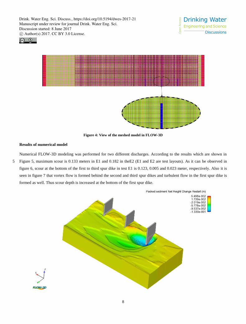
Figure 4: View of the meshed model in FLOW-3D

Results of numerical model

Numerical FLOW-3D modeling was performed for two different discharges. According to the results which are shown in

Figure 5, maximum scour is 0.133 meters in E1 and 0.182 in theE2 (E1 and E2 are test layouts). As it can be observed in 5

figure 6, scour at the bottom of the first to third spur dike in test E1 is 0.123, 0.005 and 0.023 meter, respectively. Also it is

seen in figure 7 that vortex flow is formed behind the second and third spur dikes and turbulent flow in the first spur dike is

formed as well. Thus scour depth is increased at the bottom of the first spur dike.


DiscussionsOpe

n Acc

ess


9

Figure 5: Numerical modeling results of bed deformation in E1 test, Flow direction: Right to left

Figure 6: Scour at bottom of the spur dikes in E1 test (a) first spur dike (b) second spur dike (c) third spur dike in FLOW-3D

Figure 7: The flow vortices in vicinity of the spur dikes in E1 test 5


DiscussionsOpe

n Acc

ess


10

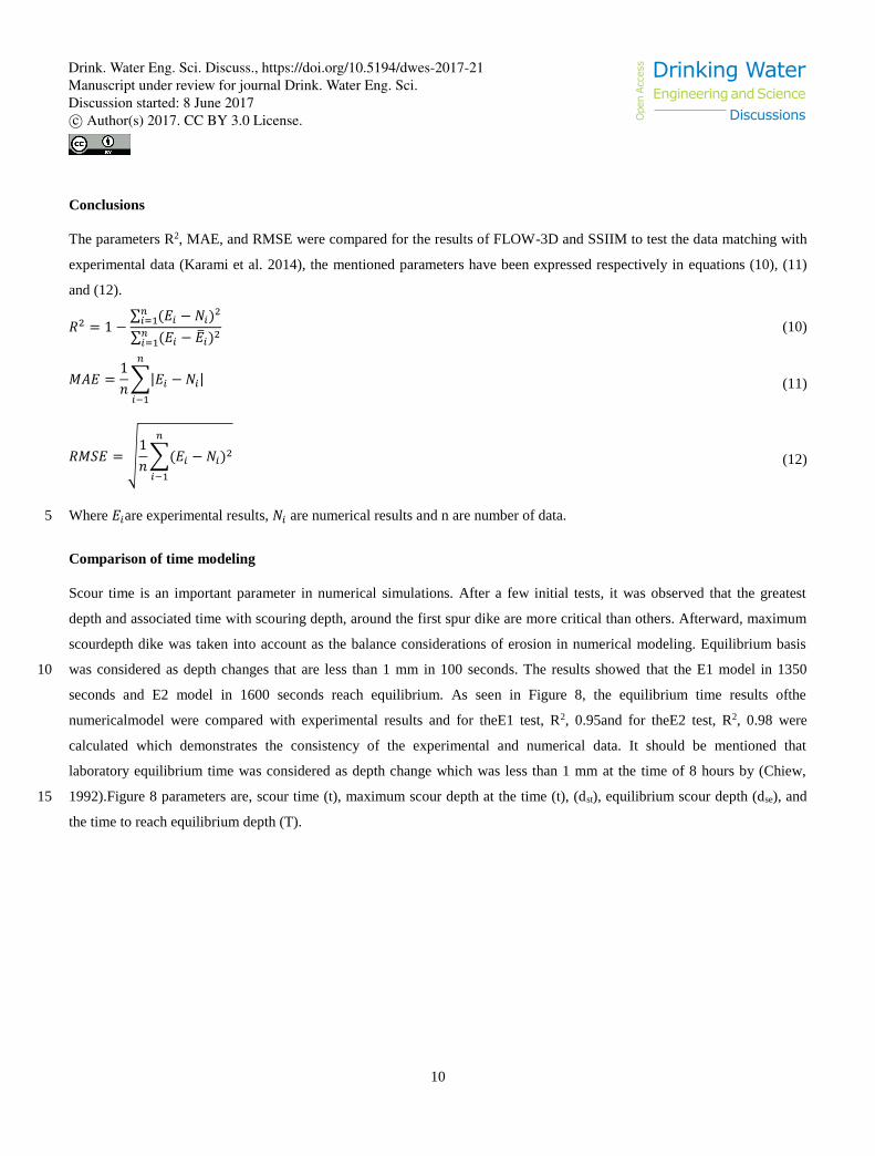
Conclusions

The parameters R2, MAE, and RMSE were compared for the results of FLOW-3D and SSIIM to test the data matching with

experimental data (Karami et al. 2014), the mentioned parameters have been expressed respectively in equations (10), (11)

and (12).

𝑅2 = 1 −∑ (𝐸𝑖 − 𝑁𝑖)

2𝑛𝑖=1

∑ (𝐸𝑖 − �̅�𝑖)2𝑛𝑖=1

(10)

𝑀𝐴𝐸 =1

𝑛∑|𝐸𝑖 − 𝑁𝑖|

𝑛

𝑖−1

(11)

𝑅𝑀𝑆𝐸 = √1

𝑛∑(𝐸𝑖 − 𝑁𝑖)

2

𝑛

𝑖−1

(12)

Where 𝐸𝑖are experimental results, 𝑁𝑖 are numerical results and n are number of data. 5

Comparison of time modeling

Scour time is an important parameter in numerical simulations. After a few initial tests, it was observed that the greatest

depth and associated time with scouring depth, around the first spur dike are more critical than others. Afterward, maximum

scourdepth dike was taken into account as the balance considerations of erosion in numerical modeling. Equilibrium basis

was considered as depth changes that are less than 1 mm in 100 seconds. The results showed that the E1 model in 1350 10

seconds and E2 model in 1600 seconds reach equilibrium. As seen in Figure 8, the equilibrium time results ofthe

numericalmodel were compared with experimental results and for theE1 test, R2, 0.95and for theE2 test, R2, 0.98 were

calculated which demonstrates the consistency of the experimental and numerical data. It should be mentioned that

laboratory equilibrium time was considered as depth change which was less than 1 mm at the time of 8 hours by (Chiew,

1992).Figure 8 parameters are, scour time (t), maximum scour depth at the time (t), (dst), equilibrium scour depth (dse), and 15

the time to reach equilibrium depth (T).


DiscussionsOpe

n Acc

ess


11

Figure 8: Dimensionless graph of equilibrium time of scouring in (a: Left) E1 test and (b: Right) E2 test in FLOW-3D

Hydraulic comparisons (SSIIM, Flow3D, Experimental)

With the aim of calibration of CFD flow simulation model results, and the experimental results used in this way that the

speed of 50 points in Z (level), equal to 2 cm above the bed, measured in theE2 test for properties. These speeds are at the

distances 5.56, 59.5, 6.16, 6.41 and 6.66 meters, which are shown in Figure 9.The results showed that k-ɛ turbulence model 5

with some RNG extensions indicates the most concordance like software SSIIM (Karami et al. 2014) with experimental

results. Figure 9 shows the absolute simulated speed comparison between two software, FLOW-3D, and SSIIM and absolute

measured speed. From this figure, it can be concluded that the CFD model simulated the flow with sufficient accuracy. Also,

quantitative comparisons results showed that FLOW-3D software with R2, 0.89 and SSIIM software with R2, 0.94, has the

capability for hydraulic flow simulation and there is not much difference between them. 10


DiscussionsOpe

n Acc

ess


12

Figure 9: CFD model comparison with experimental results

Sediment comparisons

In this study, the final results of FLOW-3D numerical model results were compared with experimental results and the SSIIM

model results. Results showed that due to the sub-critical flow, secondary flow strength and vortices from the beginning of 5

the first spur dike appears and morphological contract changes gradually. Considering that the contraction in both tests is

less than the maximum contraction and specific energy in contraction is larger than minimum specific energy. Flow depth

reduces a little in contraction and flows regime does not change. The results of both software and experimental results also

confirm this situation. With the aim of quantitative investigation of the bed changes result, experimental and software result

were compared in transverse and longitudinal sections. Two cross-sectional and longitudinal sections selected in parts after 10

contraction and in total, scouring in 80 points, in E1 and E2 tests as shown in Figure 10 and Figure 11, were examined. In

Table 4 scour depth in this 80 points in each test were compared with experimental results. Scour depth inthe bottom of the

first to third spur dikes also mentioned in this table. The results show that, in theE1 test, theFLOW-3D model is more

accurate than SSIIM model while in test E2, FLOW-3D model accuracy is very low and unacceptable. It seems that this

huge difference is due to the variations in U/Ucr. So that, FLOW-3D model calibrated in Test 1 for U/Ucr equals to 0.65 and 15

if this value changes, considering its importance, re-calibration of the model required. As a result, calibrated model of

FLOW-3D software can be used just at the same discharge.


DiscussionsOpe

n Acc

ess


13

Figure 10: Bed changes comparison of the FLOW-3D results in E1 test with SSIIM and experimental results

(a) X=6.16 (b) X=6.41 (c) Y=0.15 (d) Y=0.35

Table 4: Comparison of the scouring amount in FLOW-3D model with SSIIM model and experimental data

R2 RMSE MAE ds3 ds2 ds1 Test

- - - 0.026 0 0.156 Experimental

E1 0.6416 0.0214 0.0162 0.023 0.005 0.123 Flow3D

0.5754 0.0233 0.0151 0.013 0.033 0.101 SSIIM

- - - 0.072 0.029 0.225 Experimental

E2 0.1599 0.06596 0.0503 0.0321 0.0177 0.1785 Flow3D

0.4240 0.0546 0.0424 0.066 0.033 0.2122 SSIIM

5


DiscussionsOpe

n Acc

ess


14

Figure 11: Bed changes comparison of the FLOW-3D results in E2 test with SSIIM and experimental results

(a) X=6.16 (b) X=6.41 (c) Y=0.15 (d) Y=0.35

Summary and Conclusions

In this study, the accuracy of the FLOW-3D software versus SSIIM software (Karami et al., 2014) was evaluated by 5

comparing their model results with experimental data. To do this, the research conducted by (Karami et al., 2014) was used,

which was performed experimentally and numerically. Van Rijn sediment model is also examined, which recently added to

the FLOW-3D Model.


DiscussionsOpe

n Acc

ess


15

The results showed that Froude number and U/Ucr ratio affect the accuracy of the models. Thus, with discharge increase,

models need to be re-calibrated. Also, by using a calibrated FLOW-3D model calculation accuracy of the scour depth at the

bottom of the spur dikes will be better and accuracy in the modelling of the surface morphology improves more than SSIIM

software (Karami et al., 2014), scour at the bottom of the first, second and third spur dike, 7, 80 and 40 percent improves.

The difference in calibrated and the model which need re-calibration FLOW-3D software could be due to the calculations of 5

boundary conditions or time destruction in solving differential equations by finite volume method.

References

Kuhnle, R. A., Alonso, C. V., & Shields Jr, F. D. (2002), Local scour associated with angled spur dikes. Journal of Hydraulic

Engineering, 128(12), 1087-1093.

Klingeman, P. C., Kehe, S. M., & Owusu, Y. A. (1984), Stream bank erosion protection and channel scour manipulation 10

using rock fill dikes and gabions.

Ahmad, M. (1951), Spacing and protection of spurs for bank protection, Civil Engineering and Publication Review, 46, 3-7.

Ahmad, M. (1953), Experiments on design and behaviour of spur dikes. In Proceedings: Minnesota International Hydraulic

Convention (pp. 145-159). ASCE.

Garde, R., Subramanya, K., & Nambudripad, K. D. (1961), Study of scour around spurdikes. Journal of the Hydraulics 15

Division, 86, 23-37.

Gill, M. A. (1972), Erosion of sand beds around spur dikes, Journal of the Hydraulics Division, 98(hy9).

Richardson, E. V., Stevens, M. A., & Simons, D. B. (1975), the design of spurs for river training, In Proceeding of the 15th

Congress of the International Association for Hydraulic Research, IAHR, Basil (Vol. 2, pp. 382-388).

Rajaratnam, N., & Nwachukwu, B. A. (1983), Erosion near groyne-like structures, Journal of hydraulic Research, 21(4), 20

277-287.

Shields Jr, F. D., Cooper, C. M., & Knight, S. S. (1995), Experiment in stream restoration. Journal of Hydraulic

Engineering, 121(6), 494-502.

Kuhnle, R. A., Alonso, C. V., & Shields, F. D. (1999), The geometry of scour holes associated with 90 spur dikes. Journal of

Hydraulic Engineering, 125(9), 972-978. 25

Kothyari, U. C., & RangaRaju, K. G. (2001), Scour around spur dikes and bridge abutments. Journal of hydraulic

research, 39(4), 367-374.

Barbhuiya, A. K., & Dey, S. (2004). Local scour at abutments: A review. Sadhana, 29(5), 449-476.


DiscussionsOpe

n Acc

ess


16

Kang, J., Yeo, H., Kim, S., & Ji, U. (2011). Experimental investigation on the local scours characteristics around groynes

using a hydraulic model. Water and Environment Journal, 25(2), 181-191.

Chang, Y. L., Hsieh, T. Y., Chen, C. H., & Yang, J. C. (2013), Two-Dimensional Numerical Investigation for Short-and

Long-Term Effects of Spur Dikes on Weighted Usable Area of Rhinogobius candidianus (Goby), Journal of Hydraulic

Engineering, 139(12), 1297-1303. 5

Karami, H., Basser, H., Ardeshir, A., & Hosseini, S. H. (2014), Verification of numerical study of scour around spur dikes

using experimental data. Water and Environment Journal, 28(1), 124-134.

Mendoza-Cabrales, C. (1993). Computation of flow past a cylinder mounted on a flat plate. In Hydraulic Engineering (pp.

899-904), ASCE.

Acharya, A., &Duan, J. G. (2013), Three-dimensional simulation of the flow field around series of spur dikes. International 10

Refereed Journal of Engineering and Science (IRJES), 2, 36-57.

Duan, J. G., & Nanda, S. K. (2006), Two-dimensional depth-averaged model simulation of suspended sediment

concentration distribution in a groyne field, Journal of Hydrology, 327(3), 426-437.

Kuhnle, R. A., Jia, Y., & Alonso, C. V. (2008), Measured and simulated flow near a submerged spur dike. Journal of

Hydraulic Engineering, 134(7), 916-924. 15

An, S., Ku, H., & Julien, P. Y. (2015), Numerical modeling of local scour caused by submerged jets, Maejo International

Journal of Science and Technology, 9(3), 328.

Li, D., Shi, B., Wu, G., & Liang, B. (2016), Numerical Simulation of Near shore Submarine Pipeline Scour under Storm

Surge Condition, In The 26th International Ocean and Polar Engineering Conference. International Society of Offshore and

Polar Engineers. 20

Shamohamadi, B., & Mahboodi, A. (2016), Analyzing Parameters Influencing Scour Bed in Confluence Channels Using

Flow3D Numerical Model. Civil Engineering Journal, 2(10), 529-537.

Van Rijn, L. C. (1987). Mathematical modeling of morphological processes in the case of suspended sediment transport (pp.

Communication-No). Delft: Water loopkundig Laboratorium

Mastbergen, D. R., & Van Den Berg, J. H. (2003), Breaching in fine sands and the generation of sustained turbidity currents 25

in submarine canyons, Sedimentology, 50(4), 625-637.

Olsen, N. R. B. (2009), a three-dimensional numerical model for simulation of sediment movements in water intakes with a

multiblock option. Department of Hydraulic and Environmental Engineering: the Norwegian University of Science and

Technology.

Chiew, Y. M. (1992). Scour protection at bridge piers, Journal of Hydraulic Engineering, 118(9), 1260-1269 30


DiscussionsOpe

n Acc

ess


Numerical scour modeling around parallel spur dikes in ... · 1 Numerical scour modeling around...

Documents

Transcript of Numerical scour modeling around parallel spur dikes in ... · 1 Numerical scour modeling around...