Investigation and improvment of noise, vibration and ...
198
Wayne State University DigitalCommons@WayneState Wayne State University Dissertations 1-1-2012 Investigation and improvment of noise, vibration and harshness(nvh) properties of automotive panels Mohammad Al zubi Wayne State University, Follow this and additional works at: hp://digitalcommons.wayne.edu/oa_dissertations is Open Access Dissertation is brought to you for free and open access by DigitalCommons@WayneState. It has been accepted for inclusion in Wayne State University Dissertations by an authorized administrator of DigitalCommons@WayneState. Recommended Citation Al zubi, Mohammad, "Investigation and improvment of noise, vibration and harshness(nvh) properties of automotive panels" (2012). Wayne State University Dissertations. Paper 527.
Transcript of Investigation and improvment of noise, vibration and ...
Wayne State UniversityDigitalCommons@WayneState
Wayne State University Dissertations
1-1-2012
Investigation and improvment of noise, vibrationand harshness(nvh) properties of automotivepanelsMohammad Al zubiWayne State University,
Follow this and additional works at: http://digitalcommons.wayne.edu/oa_dissertations
This Open Access Dissertation is brought to you for free and open access by DigitalCommons@WayneState. It has been accepted for inclusion inWayne State University Dissertations by an authorized administrator of DigitalCommons@WayneState.
Recommended CitationAl zubi, Mohammad, "Investigation and improvment of noise, vibration and harshness(nvh) properties of automotive panels" (2012).Wayne State University Dissertations. Paper 527.

INVESTIGATION AND IMPROVEMENT OF NOISE, VIBRATION AND HARSHNESS
(NVH) PROPERTIES OF AUTOMOTIVE PANELS
by
MOHAMMAD AL-ZUBI
DISSERTATION
Submitted to the Graduate School
of Wayne State University,
Detroit, Michigan
in partial fulfillment of the requirements
for the degree of
DOCTOR OF PHILOSOPHY
2012
MAJOR: MECHANICAL ENGINEERING
Approved by:
. .
Advisor Date
. .
. .
. .

ii
DEDICATION
To my parents who had me in all their prayers.
To my beloved wife, I could not have done this without her support
To my daughter Lina, and son Abdullah. They saw little of their father
in the last couple of months.

iii
ACKNOWLEDGEMENT
I would like to start by thanking the almighty Allah for granting me the will and patience to do
this work.
I am sincerely and heartily grateful to my advisor, Dr. E.O. Ayorinde, for the support and
guidance he showed me throughout the period I spent under his supervision and through my
dissertation writing. I am sure it would have not been possible without his help and support. I
would like to thank my committee members Dr. Trilochan Singh, Dr. Golam Newaz and Dr
Hwai-Chung Wu. I benefited greatly from the advice of every single one of them.
Besides I would like to thank my colleagues, Mehmet Akif Dundar , and Manjinder Singh for
their cooperation and support during this work.

iv
TABLE OF CONTENTS
Dedication……………………………………………………………………………... ii
Acknowledgement…………………………………………………………………………. iii
List of Figures……….……………………………………………………………………... viii
List of Tables…….………………………………………………………………………… xv
CHAPTER 1 BACKGROUND AND INTRODUCTION……………………………… 1
CHAPTER 2 LITRUTURE SURVEY………………………………………………….. 6
CHAPTER 3 OBJECTIVES AND THEORY………………………………………….. 13
3.1 OBJECTIVES OF THE RESEARCH………………………………………
3.2 INTRODUCTION TO VIBRATION OF PLATES………………………...
3.3 GENERAL PLATES VIBRATION………………………………………….
3.4 VIBRATION OF CIRCULAR PLATES……………………………………
3.5 ACOUSTICS THEORY………………………………………………………
3.5.1 DYNAMICS OF ACOUSTIC PLANE WAVES………………………..
3.5.2 ACOUSTIC TRANSMISSION IN THICK FINITE MEDIUM………...
3.5.3. ANALYSIS FOR AIR PROPAGATION CONSTANT, γ, AND
WAVE IMPEDANCE, W……………………………………………………...
3.5.4 DEDUCTION OF ABSORPTION AND REFLECTION
COEFFICIENTS……………………………………………………………….
3.5.5 ACOUSTIC ANALYSIS OF RIGID POROUS MATERIALS…………
13
14
16
20
24
25
26
27
28
29

v
CHAPTER 4 EXPERIMENTAL WORK………………………………………………. 33
4.1 MATERIALS………………………………..……………………………….
4.1.1 FABRIC MATERIALS…………………………………………………
4.1.2 FOAM MATERIALS…………………………………………………..
4.1.3 HONEYCOMB MATERIALS…………………………………………
4.1.4 MONOLITHIC AND SANDWICH MATERIALS……………………
4.1.5 PERIODIC CELLULAR MATERIAL STRUCTURES (PCMS)
MATERIALS…………………………………………………………………
4.1.6 GENERAL PERIODIC MATERIALS…………………………………
4.2 APPARATUS…………..………………………………………………….....
4.2.1 VIBRATION TEST APPARATUS………………………………..……
4.2.2 ACOUSTICS TEST APARATUS……………………………..………..
4.3 EXPERIMENTAL TEST PROCEDURES…..…………………………….
4.3.1 VIBRATION TEST PROCEDURE…………………………………...
4.3.2 PULSE REFLEX™ MODAL ANALYSIS……………………………
4.3.3 ACOUSTIC TEST PROCEDURE…………………………………….
33
34
35
36
38
40
40
41
42
43
45
45
51
55
CHAPTER 5 NUMRICAL WORK……………………………………………………... 60
5.1 CALCULATIONS…..………………………………………………………..
5.2 FINITE ELEMENT………………………………………………………...
5.3 MATLAB……………………………………………………………………
60
61
64
CHAPTER 6 RESULTS AND DISCUSSION………………………………………….. 66
6.1 INTRODUCTION………………………………………………...………...
6.2 ACOUSTICS RESULTS…………………………………………………...
66
66

vi
6.2.1 FABRIC MATERIALS………………………………………………..
6.2.2 FOAM MATERIALS………………………………………………….
6.2.3 HONEYCOMB MATERIALS………………………………………...
6.2.4 MONOLITHIC AND SANDWICH MATERIALS……………………
6.2.5 PERIODIC CELLULAR MATERIAL STRUCTURES (PCMS)
MATERIALS………………………………………………………………...
6.2.6 GENERAL PERIODIC MATERIALS………………………………...
6.3VIBRATION RESULTS………………..……………………………………
6.3.1 HONEYCOMB MATERIA……………………………………………
6.3.2 MONOLITHIC AND SANDWICH MATERIALS……………….…...
6.3.3 PERIODIC CELLULAR MATERIAL STRUCTURES (PCMS)
MATERIALS………………………………………………………………...
6.3.4 GENERAL PERIODIC MATERIALS………………………..……….
6.4 PARAMETRIC STUDIES…………..………………………………………
6.4.1 PARAMETRIC STUDIS FOR SOUND ABSORPTION
COEFFICIENT……………………………………………………………….
6.4.2 PARAMETRIC STUDIES FOR VIBRATION………………………..
66
67
69
71
76
77
79
80
88
110
121
127
127
132
CHAPTER 7 CONCLUSIONS AND FUTURE WORK………………………………. 146
7.1 CONCLUSIONS…………..…………………………………………………
7.2 FUTURE WORK…………………………………………………..………...
146
149
Appendix A: Matlab Code to Calculate Sound Absorption Coefficient for Porous
Rigid Materials………………………………………………….......……...
157

vii
Appendix B: Matlab Code to Calculate Natural Frequencies and Mode Shapes for
Lexan……………………………………..…………………………………
152
Appendix C: Eigen Value Output for One Layer Lexan with Large
Holes..……………………………………………………………………..
155
Appendix D: Vibration Results for One More Sample From each Group Described
in the Dissertation with Same Sequence………………………………….
160
References…………………………….…………………………………………………… 170
Abstract…………………………...………………………………………………............. 178
Autobiographical Statement……………………….…………………………………….. 179

viii
LIST OF FIGURES
Figure 3.1: Element of a vibrating plate………………….………………………………… 16
Figure 3.2: Model of deformed coordinates in plate vibration…………………………… 21
Figure 4.1: Fabric tested Materials…………………………………………………………. 34
Figure 4.2: Tested foam materials…………………………………………………………... 36
Figure 4.3 Tested honeycomb materials……………………………………………………. 37
Figure 4.4: Tested monolithic and sandwich materials……………………………………... 39
Figure 4.5: Tested periodic cellular material structures (PCMS) materials………………… 40
Figure 4.6: Tested general periodic material structures…………………………………….. 41
Figure 4.7: Vibration test apparatus with its components…………………………………... 42
Figure 4.8: A sketch for the vibration apparatus………..…………………………………... 43
Figure 4.9: Geometry drawn inside Pulse, the hammer is roving, while accelerometer is
fixed at point1…………………..………………………………………………
43
Figure 4.10: Acoustic test apparatus………………………………………………………... 44
Figure 4.11: Cut-away diagram of the impedance measurement tube, showing the incident
and reflected components of the stationary-random signal…………………....
45
Figure 4.12: The first step in opening Modal analysis application from Pulse…………….. 46
Figure 4.13: Selection of roving hammer test……………………………………………..... 46
Figure 4.14: Detection of Transducer electronic database………………………………….. 47
Figure 4.15: Trigger level setup selection…………………………………………………... 48
Figure 4.16: Setting the trigger level manually……………………………………………... 49
Figure 4.17: Response window shows the signal decay with time………………………..... 50
Figure 4:18: Geometry imported from Pulse to Reflex…………………………………….. 52

ix
Figure 4.19: Measurement Validation step in Reflex………………………………………. 52
Figure 4.20: Parameter estimation setup in Reflex (auto selection of frequency range)….... 53
Figure 4.21: Mode selection in Reflex (natural frequencies and mode shapes)……………. 54
Figure 4.22: Analysis validation includes the first two modes……………………………... 55
Figure 6.1: Absorption coefficient versus frequency for fabric materials………………….. 66
Figure 6.2: Absorption coefficient versus frequency for foam materials………………….. 68
Figure 6.3: Absorption coefficient versus frequency for honeycomb materials…………..... 70
Figure 6.4: Absorption coefficient versus frequency for sandwich materials…………….... 72
Figure 6.5: Sound absorption of two different Lexan configurations……………………..... 72
Figure 6.6: Absorption coefficient for 2-layer solid Lexan versus single- Layer one…….... 73
Figure: 6.7 Absorption coefficient for sold 2-layer Lexan with small holes versus one with
large holes ……………………….……………………………………………..
74
Figure 6.8: Absorption coefficient for 2-layer solid Lexan versus one with an air-gap of
18mm……………….…………………………………………………………..
75
Figure 6.9: Sound absorption for PCMS Materials…………………………………………. 76
Figure 6.10: Sound absorption for two periodic materials (large size only)………………... 77
Figure 6.11: Absorption coefficient versus frequency for Aluminum nuts double staggered
micropillars………...…………..…………………………………...................
78
Figure 6.12: Figure 6.12: Stability diagram shows the 1st three natural frequencies (Nomex
HC)…………………………………………………….....................................
80
Figure 6.13: FRF, Coherence and phase for (Nomex HC)…………………………………. 81
Figure 6.14: 1st three mode shapes (displacement and stress, Nomex HC)……………….... 81
Figure 6.15: Maximum deflection for the 1st three modes (Nomex HC)…………………... 82

x
Figure 6.16: Damping ratio for the 1st three modes (Nomex HC)………………………….. 82
Figure 6.17: Compatibility between experiment and FEM results (Nomex HC)…………... 83
Figure 6.18: Comparisons between the numbers of elements (Honeycomb group)………... 85
Figure 6.19: Comparison between natural frequencies for the 1st three modes (Honeycomb
group)……………………….……………………………...............................
86
Figure 6.20: Comparison between maximum deflections for the 1st three modes
(Honeycomb group)………...……………………..………………………......
87
Figure 6.21: Comparison between damping ratios for the 1st three modes (Honeycomb
group)…………………..…...……………………………………………........
87
Figure 6.22: Comparison between modal densities (Honeycomb group)…………………... 88
Figure 6.23: Stability diagram shows the 1st three natural frequencies (1 Layer Lexan
w/large holes)…….…………………………………………………………....
89
Figure 6.24: FRF, Coherence and phase (1Layer Lexan w/large holes)……………………. 90
Figure 6.25: FRF results from RADIOSS (1 Layer Lexan w/large holes)…………………. 91
Figure 6.26: 1st three mode shapes (displacement contour, 1 Layer Lexan w/large holes)... 91
Figure 6.27: Maximum deflection for the 1st three modes (1 Layer Lexan w/large holes).... 92
Figure 6.28: Damping ratio for the 1st three modes (1 Layer Lexan w/large holes)………... 92
Figure 6.29: Compatibility between experiment and FEM results (1 Layer Lexan w/large
holes)…………...….…………………………………………………..……....
93
Figure 6.30: Stability diagram shows the 1st three natural frequencies (USIL Light)…….... 94
Figure 6.31: FRF, Coherence and phase (USIL Light)……………………………………... 94
Figure 6.32: FRF results from RADIOSS (USIL Light)…………………………………… 95
Figure 6.33: 1st three mode shapes (displacement contour, USIL Light)………………….. 95

xi
Figure 6.34: 1st three mode shapes using Matlab (USIL Light)…………………………….. 96
Figure 6.35: Maximum deflection for the 1st three modes (USIL Light)………………….... 97
Figure 6.36: Damping ratio for the 1st three modes (USIL Light)………………………….. 97
Figure 6.37: Compatibility between experiment and numerical methods results (USIL
Light)……………...……………………………………………………….......
98
Figure 6.38: Number of elements for monolithic materials……………………………….... 101
Figure 6.39: Comparison between natural frequencies for the 1st three modes (monolithic
materials)………....……………………………………………………………
102
Figure 6.40: Comparison between maximum deflections for the 1st three modes
(monolithic materials)……………………...……………………...........
103
Figure 6.41: Comparison between damping ratios for the 1st three modes(monolithic
materials)………………………………………………………………………
104
Figure 6.42: Comparison between modal densities(monolithic materials)………………..... 105
Figure 6.43: Comparison between numbers of elements(sandwich materials)……………... 106
Figure 6.44: Comparison between natural frequencies for the 1st three modes(sandwich
materials)…………………………………………………….………………...
107
Figure 6.45: Comparison between maximum deflections for the 1st three modes(sandwich
materials)………….…………………………………………………………...
108
Figure 6.46: Comparison between damping ratios for the 1st three modes(sandwich
materials)……………........................................................................................
109
Figure 6.47: Comparison between modal densities(sandwich materials)………………....... 110
Figure 6.48: Stability diagram shows the first three natural frequencies (Aluminum
prismatic microtruss)…......................................................................................
111

xii
Figure 6.49: FRF, Coherence and phase (Aluminum prismatic microtruss)…….................. 112
Figure 6.50: FRF results from RADIOSS (Aluminum prismatic microtruss)………............ 112
Figure 6.51: 1st three mode shapes (displacement contour, Aluminum prismatic
microtruss)……….……………………………………………………………
113
Figure 6.52: Maximum deflection for the 1st three modes(Aluminum prismatic
microtruss)…….................................................................................................
114
Figure 6.53: Damping ratio for the 1st three modes(Aluminum prismatic
microtruss)……...…………….……………………………………………….
114
Figure 6.54: Compatibility between experiment and FEM results(Aluminum prismatic
microtruss)……….............................................................................................
115
Figure 6.55: Comparison between numbers of elements(PCMS Materials)…...................... 117
Figure 6.56: Comparison between natural frequencies for the 1st three modes(PCMS
Materials).…………………………………………….………………….……
118
Figure 6.57: Comparison between maximum deflections for the 1st three modes(PCMS
Materials)……………..……….………………………………………………
119
Figure 6.58: Comparison between damping ratios for the 1st three modes(PCMS
Materials)………………………............................................................……...
119
Figure 6.59: Comparison between modal densities(PCMS Materials)…………………....... 120
Figure 6.60: Stability diagram shows the first three natural frequencies(Aluminum nuts
double staggered micropillars)……………..………………….........................
121
Figure 6.61: FRF, Coherence and phase(Aluminum nuts double staggered micropillars)…. 122
Figure 6.62: 1st three mode shapes (displacement contour,Aluminum nuts double
staggered micropillars)……………………………………….……..................
122

xiii
Figure 6.63: Maximum deflection for the 1st three modes(Aluminum nuts double
staggered micropillars)…………………….…………………..........................
123
Figure 6.64: Damping ratio for the 1st three modes(Aluminum nuts double staggered
micropillars)………..………………………………………………………….
123
Figure 6.65: Comparison between natural frequencies for the 1st three modes(Periodic
materials)…………............................................................................................
125
Figure 6.66: Comparison between maximum deflections for the 1st three modes(Periodic
materials)…......................................................................................................
126
Figure 6.67: Comparison between damping ratios for the 1st three modes (Periodic
materials)………………………………………………………………………
126
Figure 6.68: Comparison between modal densities (Periodic materials)………………….... 127
Figure 6.69: Compatibility between experimental and code results for absorption
coefficient...........................................................................................................
129
Figure 6.70: Effect of changing thickness on sound absorption……………......................... 130
Figure 6.71: The effect of porosity on sound absorption coefficient……………………….. 131
Figure 6.72: The effect of structure factor on sound absorption coefficient……………....... 132
Figure 6.73: Compatibility between experimental and FEM results for natural
frequencies……………………………..………………….…………………..
133
Figure 6.74: Effect of thickness on natural frequency………………………….................... 133
Figure 6.75: Fundamental natural frequency for different architecture……………….......... 135
Figure 6.76: Displacement contour for sample 1………………………………………….... 136
Figure 6.77: Displacement contour for sample2………………………………………......... 136
Figure 6.78: Gaps for two different aluminum samples……………………………………. 137

xiv
Figure 6.79: The change of frequency with gap…………………………………………..... 138
Figure 6.80: Change of VonMises stress with gap……………………………………......... 139
Figure 6.81: VonMises and displacement contours for Aluminum prismatic PCMS cuts
arranged according to table 6.10………..……………………………………..
140
Figure 6.82: Sample number 1 as it appears in FEM model……………………………....... 141
Figure 6.83: The first mode natural frequencies for stainless steel samples……………....... 142
Figure 6.84: The first mode VonMises stress for stainless steel samples………………....... 142
Figure 6.85: VonMises and displacement contours for Stainless steel triangular
honeycomb PCMS cuts arranged according to table 6.16……………..……...
144

xv
LIST OF TABLES
Table 3.1: Alpha values for different nodal lines and circles……………………………… 24
Table 4.1: Fabric Materials Properties……………………………………………………. 35
Table 4.2: Foam Materials properties……………………………………………………… 36
Table 4.3: Properties for Honey comb Materials………………………………………….. 38
Table 4.4: Properties of Sandwich and Monolithic Materials……………………………... 39
Table 4.5: Properties of PCMS Materials………………………………………………….. 40
Table 4.6: Properties of general periodic material structures……………………………… 41
Table 5.1 Calculated Natural frequencies for Solid Lexan………………………………... 61
Table 6.1: Comparison between honey comb samples according to number of nodes,
elements and element type, with the modal densities……...………………...…
84
Table 6.2: Vibration results for Honeycomb structures…………………………………... 84
Table 6.3 Comparison between Sandwich and monolithic samples according to number
of nodes, elements and element type, with the modal densities…………………
99
Table 6.4: Vibration results for Sandwich and Monolithic structures……………………... 100
Table 6.5: Comparison between sandwich and monolithic samples according to number
of nodes, elements and element type, with the modal densities…………………
116
Table 6.6: Vibration results for PCMS materials………………………………………….. 116
Table 6.7: Vibration results for General periodic materials……………………………… 124
Table 6.8: The first three resonance frequencies for different Lexan architecture………… 135
Table 6.9: Natural frequencies and VonMises stress for the CMI samples……………….. 137
Table 6.10: Results for different samples from FEM simulations for aluminum samples… 138

xvi
Table 6.11: Results for different samples from FEM simulations for stainless steel
samples…………………………………………………………………………..
141
Table 6.12: Perentage varaitions for the (frequency and strees)from the original sample… 145

1
CHAPTER 1
BACKGROUND AND INTRODUCTION
Vehicle manufacturers initially relied on horsepower and speed performances as “standout
qualities” to sell their products, but as time progressed, it became increasingly clear that
customers were very much concerned about their comfort as they drove the vehicles. In the late
seventies, requirements for driver and passenger comfort were increased significantly. Since
then, a large amount of effort has been invested into the improvement of the technology of noise
and vibration reduction and containment. It became no longer adequate to simply cram as much
insulation as possible into the panels (door, roof, floor, etc.,) to abate rattling movements and
achieve quiet. Saha (in Anon [1]) recalled that the earlier power trains were so noisy that one
could not even hear the wind noise at all within the vehicle. When success was achieved in
quietening down the power train, the wind noise then became the major challenge. He remarked
that historical data shows that the persistent drive towards ever-increasing noise and vibration
performance has in fact been driven mainly by customer demand rather than legal and regulatory
requirements and standards. Kropp (in Anon [1]) summarized that “noise and vibration have
become a statement of car quality”. He further explained that people buy cars to get from one
point to another – reliably and comfortably, but that they also want a quiet ride for their money,
and for example want to listen to the radio without being disturbed by a lot of noise.
A novel vibro-acoustic containment method [2] builds on the discovery that plate flexural
vibrations can be effectively stopped from reflecting back by terminating the plate with a small
layer or wedge of damping material, thus effectively ending the life of such a propagating wave.
Accordingly, acoustic effects emanating from the vibration of such a plate are also practically
terminated. This approach is in its infancy, and is not covered in the work of this dissertation.

2
Yet another novel approach is the use of micro honeycomb constructions [3], whereby the
honeycomb comprises micrometer size cylinders through which sound can travel and interact
with the material in shear, and thus get practically dully dissipated before or by the time that it
arrives at the end of the protrusion. The energy destruction mechanism is through shearing rather
than absorption.
This work concentrates on the automotive panel for good reason. The automotive panel is of
significant importance, as there are several kinds [4] in a typical vehicle. Which combination of
panels are used in a particular application would depend on the geometry of the vehicle –
whether salon, truck, cab-style, station wagon, convertible, or some other. These panels
accordingly include the full floor panel, cab floor panel, front side panel, car rocker panels, front
floor panels, pan panels, lower front door skins, lower rear quarter panels, under-seat floor pan
panel, roof panel, etc.
According to the importance that automotive vibro-acoustics has commanded, several
institutions in many parts of the world [1] have evolved formal study courses and vigorous
research programs in academic disciplines designed to abate noise and vibration in the
automotive environment. Examples of colleges with these programs include the Institute of
Sound and Vibration Research in the UK, Chalmers Institution of Technology in Sweden, and
the Technical University of Denmark.
The reduction of vibration and noise in and across several components and modules of the
automotive, such as the panels, doors, engine covers, seats, and others, is of primary importance.
The NVH performance may be a crucial factor in the purchase decisions of numerous buyers. In
this work, experimental and other investigations are made on monolayer, composite and periodic

3
material constructions to assess their suitability for minimal transmission of noise and vibration.
With respect to the materials and constructions that are suitable for noise and vibration
containment, some are more suitable for noise control, and some for vibration control and some
may be good in both areas. A major goal of this work is to investigate sample materials and
architectures that are more applicable in the industry and are being examined for possible
utilization, or that may be recommended for NVH amelioration.
Vehicle interior noise perceived in the passenger cabin of an automobile is one of the most
important factors in a customer’s determination of the quality and durability of the vehicle. Thus,
the reduction of interior noise is a major concern for automobile manufacturers trying to achieve
customer satisfaction and a market leadership position in the highly competitive automotive
market.
Automotive interior noise is generated by various elements such as the engine,
transmission, and climate-control system [5]. However, due to technological advancement in the
sound and vibration engineering of vehicles, the overall noise level from vehicles has been
continuously reduced, which has resulted in drawing the occupant’s attention to intermittent
noise such as buzz, squeak, and rattle (BSR) [6] [7] . A market survey reported BSR as the third
most important customer concern in cars after 3 months of ownership [8]. Thus, BSR noise is
increasingly seen as a direct indicator of vehicle quality and reliability.
The sound wave emanating from the vibrating structure alone is called “buzz”. “Squeak” is noise
originating from frictional movement between two parts, and “rattle” is noise due to the impact
of one part on another [9]. Squeak is caused by the elastic deformation of the contact surfaces
storing energy, which is released when the static friction exceeds the kinetic friction and rattle is
generated by loose or very flexible elements under forced excitation. For both squeak and rattle
4
noises, the exciting force is due mainly to the road surface, which forces components to vibrate
vertically. The main causes of BSR noise can be categorized as structural deficiencies, non-
matching material pairs, and bad geometrical alignment [8] and [9]. The basic cause of BSR
noise is the relative motion of structural components exceeding a threshold value.
Since BSR is noticed by customers, manufacturers have worked out many specifications
for assemblies and components. The physics of the phenomena have been reported earlier, but
direct applications relating to the BSR problem have only been published recently [10].
. The main issues in BSR are the lack of real test standards and nebulous acceptance criteria
written into existing specifications [11]. Traditionally, vehicle product evaluation from the BSR
perspective depends heavily on physical testing and engineering experience.
Most vehicle manufacturers detect and fix BSR problems with the road test as a result of
various excitation sources, complex generation mechanisms, and responses of human subjects.
To improve the situation, it has been suggested [9] that (1) find and fix BSR problems for
modules instead of a full vehicle to address the problems in the early stage; (2) design vibration
exciters to perfectly reproduce input signals to the vehicle from the road; (3) develop techniques
to automatically localize the source region of BSR in spite of various potential noise sources; and
(4) to establish a sound quality evaluation system allowing for subjective responses to BSR. In a
study [7] a BSR evaluation system and procedures were developed for automotive interior
modules that consist of an excitation shaker and vibration jigs for the modules, acoustic-field
visualization techniques, and the evaluation of sound quality. Instrument panels, seats, and doors
are considered to be responsible for over 50% of the total BSR vehicle interior noise problems,
with the instrument panel (IP) module being the main source [8].

5
CHAPTER 2
LITERATURE SURVEY
Poisson [12] first examined the vibrations of circular plates investigating the three cases of
fixed, simply supported and free edges. He analyzed theoretically some of the symmetrical
modes of vibrations and calculated the ratios of the radii of the nodal circles to the radius of the
plate when the vibrating plate had no nodal diameter or one or two nodal circles. The full theory
of the vibration of a free circular plate was later developed by the Kirchhoff [13]. Kirchhoff
extended the Poisson’s results for the vibration of free plate by calculating six ratios of the radii
with one, two or three nodal diameters. Lord Rayleigh [14] developed a general theory of these
vibrations and highlighted the low frequencies of thin plates; while Lamb [15] gave a summary
of the theoretical work to date. The general Rayleigh method is based on the energy principle,
while a latter modification by Ritz uses a sum of functions to represent the vibratory deflection,
while the method by Bolotin utilizes asymptotic approximations to the eigen functions.
Airey [16] studied the vibrations of circular plates and, like Rayleigh, also explored their
treatment with Bessel functions, and generated a method of solving the plate equations to yield
the characteristic equation roots, and the radii of the nodal circles for any vibration mode.
Timoshenko [17] analyzed the transverse vibration of rectangular and circular isotropic plates
under different boundary conditions, obtaining natural frequency formulas. Wood [18]
experimentally investigated the free transverse vibration of circular plates having significant
thickness. These plates have high transverse vibration natural frequencies that may even be
beyond the human hearing.

6
Iguchi [19] explored the vibrations variously constrained plate, focusing in a latter work
[20] on the completely free boundary condition, and employing the summation of symmetric and
asymmetric Levy expansions to obtain exact solutions for the Eigen functions. Warburton [21]
utilized characteristic beam vibration functions in Rayleigh’s method to evolve simple
approximate expressions for natural frequencies of thin, isotropic rectangular plates under
different boundary conditions and various ratios of the plate side lengths. This method saves
significantly on the time and computer resources normally utilized by many other methods such
as the Ritz, Bolotin’s, series solutions, finite difference and finite element method. An extensive
work, embracing many boundary conditions and anisotropic material behavior, was presented by
Lekhnitskii, Tsai and Cheron [22] for mode shapes and natural frequencies. A comprehensive
work on the vibration of plates, commissioned by NASA, was published by Leissa [23]. Zelenov
and Elektrova [24] utilized experimental vibration results and analysis to estimate the elastic
constants of an isotropic circular plate having different boundary conditions. Gorman et al.
[25][26][27] analyzed the free vibration of rectangular plates, utilizing symmetries and
simplified functions. Dickinson et al. [28] advanced Warburton’s approach to especially
orthotropic plates and also inclusion of the effect of uniform, direct-in-plane force in generating
approximate formulas for natural frequencies of flexural vibration. An early example of the finite
element application may be found in the work of Dinis and Owen [29], analyzing elasto-
viscoplastic plates.
A utilitarian handbook of principles and formulas of the vibration of structural and fluid
systems was published by Blevins in 1979 [30] to facilitate finding the frequencies and mode
shapes of a wide range structures. A finite element method for the vibration analysis of
sandwich structures was presented by Connor in 1987 [31], including the effect of transverse

7
normal deformation of core. Ewins [32] published an analytical and practical work on modal
testing technology, with a mathematical model expressing the vibration properties of a structure
based on test data.
Deobald and Gibson [33] matched vibration analysis calculations with experimental data
to extract elastic constants of specimens. Bardell [34] determined the natural frequencies and
modes of a flat rectangular plate with the finite element method, utilizing boundary conditions
and presented several parameters (including the variation of frequency with the aspect ratio and
the Poisson’s ratio. Lai and Lau [35] extended the method of Deobald and Gibson [33] to
examine the full modal testing of a plate with free edges, and calculated elastic constants. Lee
and Fan [36] explored the finite element analysis of composite sandwich plates, utilizing
Mindlin’s plate theory (which assumes that shear deformation takes place, and the plate section
is deformed into the shape of a parallelepiped), and investigating the effect of the transverse
normal deformation of the core. They concluded that cores that are flexible in the transverse
normal direction tend to decrease natural frequencies without significant alteration of mode
shapes.
Galerkin’s work on damped sandwich beams was extended to the plates domain by Zhang
and Sainsbury [37], while further finite element applications may be found in the works of
Klosowski et al [38]. Klosowski [39] studied the vibrations of circular plates subjected to shock-
wave impulses. They utilized finite element analysis and compared to experimental data, with
good correlation.
Hoshino, Takura and Takahashi [40] simulated and analyzed the vibration containment of
heavy duty truck cabins with a load transfer path theory. The load paths identify load transfer

8
and warn the designer of the creation of bending moments and the location of features such as
holes on the load path. The algorithm of the theory provides insight into the way a structure is
carrying loads by identifying the material most effective in performing the load transfer. They
concluded that the floor panel is closely related to the stiffness of the front cross-member of the
floor structure,, and that discontinuities and non-uniformities in the load paths reduces the front
cross-member stiffness. Sun et al. [41] applied Statistical Energy Analysis (SEA) to the design of
car interior trims and concluded that proper design of such trims may be guided by such
analyses. Car interior pressures before and after applications of various trims confirmed the
improvements achieved. Pappada et al. [42] investigated the upgrade of damping in laminated
composite plates by embedding shape memory alloy (i.e. those which manifest this behavior
recover their pre-deformation shapes when load is removed or temperature is altered.) composite
wires in them. They found that damping always improved by this method, but found that curved
and patterned wires were more effective than straight wires. Shin and Cheong [43]
experimentally characterized buzz, squeak and rattle (BSR) noise in stationary automobiles and
stated from their results that their procedure offers a reliable method to systematically obtain
BSR data for various automotive component sources.
Earlier on, study of wall transmission loss was limited by because only the wall mass was
considered, and consequently; the results obtained only gave a basic approximation and did not
explain all the observed phenomena (e.g., critical frequency).
Elasticity was introduced in to the problem for an infinite plate by Cremer [44], revealing
the important phenomenon of critical frequency, when the wave propagation speeds of the plate
and of the fluid are equal. London [45] used the hypothesis of the infinite plate, and also
contributed how to find transmission loss in a diffuse field of a simple wall and for double wall.

9
In their treatise on sound absorbing materials, Zwikker and Kosten [46] gave an extensive
literature review with substantial data and tables on the sound absorption coefficients of several
materials. They supplied useful insight into the acoustic roles of physical features of the
materials (thickness, porosity, diameter, stiffness), thus guiding the adequate design of sound
abatement materials. Their models and theories were practical but proved unable to highlight
detailed phenomena, especially at low frequency. The work of Vogels [47] on finite plates was
equivalent to a foundation effort in modal analysis, which permitted the establishment of detailed
laws and a clearer understanding of these phenomena. Interest was stimulated in the study of
wall radiation (i.e. due to the vibration of a flexible wall), and of the influence of internal
damping of the plate. Hickman [48], who studied the infinite model of the complex plate
(sandwich), only considered the flexure and extension of the wall. Kurtze [49] enunciated a
principle of wave propagation and Watters [50] studied a basic model of sandwich behavior,
where the core acts as a spacer that has mass and transmits shear, while the skins behave as
ordinary bent plates. He obtained the impedance for such a composite plate from an equivalent
circuit analog, and the imposition of a null value on that impedance led to a bi-cubic equation for
admissible wave speeds of bending and shears waves in the plate. Maidanik [51] evaluated
impedance radiation values for the cases of single-mode excitation of the plate, or when the plate
is loaded by a diffuse field.
Free vibration analysis of a basic sandwich model was provided by Ford, Lord, and
Walker [52] with observation of a relation between dips in experimental transmission loss curves
and the resonance frequencies in both bending and dilatational modes. Sharp and Beauchamp
[53] utilized Hickman’s hypothesis to generalize the results for the case of n layers. Using the
double Fourier transform, Spronck [54] obtained an expression for the radiation impedance for a

10
general case. He mentioned non-diagonal terms in the radiation impedance matrix, which
signified an interaction of one mode with another, on account of the fluid spaces. The radiation
impedance was not obtained for the general case, but was assumed to be negligible after the
earlier observation of Sewell [55]. Incidentally, this was proved by later workers to be incorrect.
The energy expression by Ford, Lord, and Walker was corrected by Smolenski and
Krokosky [56], who compared resonance data from their further experimental work with
analytical results. They also highlighted a coincidence effect beyond the bending coincidence.
Analytic expressions for impedance and transmission loss of a sandwich panel were obtained by
Dym and Lang [57] thus facilitating comparisons with experimental data thenceforth. Guyader
and Lesueur [58] derived an analytic expression for the infinite plate transmission for the three-
layered sandwich plate, and extended it to multi-layered plates.
Many aspects of low-frequency range sound transmission were studied in detail by
Woodcock and Nicolas [59], with emphasis on the finite-size panel, its orthotropic properties and
the boundary conditions, apparently for the first time. The intermodal interaction was well
highlighted. Pates, Mei and Shirahatti [60] compared coupled BEM/FEM analysis with existing
classical modal approximation, and experimental solutions for isotropic panels were found to be
accurate and reliable solutions to complex problems. Transmission loss data for isotropic and
composite panels were analyzed and compared. Lamination study was also done to illustrate the
effect of orientation angle on overall transmission loss.
In a model based on the compilation of the impedances encountered by an acoustic wave
as it propagates through the wall, Fringuellino and Guglielmone [61] proposed a formula for the

11
transmission loss of multilayered walls. The characteristic impedance and the propagation
constant of each layer are utilized as input parameters.
Lim [62] studied the radiated noise contributions of automotive body panels to the interior
sound pressure levels, with an approximate spectral formulation model, and also applying it to a
real car. The results showed structural panels that contributed most significantly to the interior
noise spectra, and thus which should be prime candidates for design modifications to reduce the
interior noise levels.
Hills, Mace and Ferguson [63] investigated the statistical variability of noise response in
automotive interiors. They suggested reasonable assumptions, and concluded that changes in
specification such as trim, minor body modifications and, in particular, tire and rim type might
cause significant variability from one specification to another, thus providing a challenge to the
engineer’s effort to produce robust, low noise products.
Binxing et al. [64] combined various numerical calculation methods to model and analyze
the acoustic characteristics of a heavy truck cab. They concluded that various numerical
calculation methods, such as FEM, BEM and SEA, can be rigorously combined to model and
analyze the acoustic characteristics of vehicles. They also concluded that the sound quality of
the cab can be improved after acoustic topology optimization. The interior noise level was
reduced by a few decibels.

12
CHAPTER 3
OBJECTIVES AND THEORY
The traditional method for constructing the automotive panel structure has been typically to
layer a metal panel outer member with a visco-elastic damping layer, then a porous layer, and
then a rubber/plastic layer in order to affect improved vibro-acoustic performance. More recently
[65], efforts have been directed in the industry towards improving the nature and/or architecture
of the panel material itself, such that extra costs associated with added materials and the
fabrication and assembly labor costs that are involved are saved as much as possible, and yet
such panels have good vibration and acoustics performances.
From the existing literature, it is obvious that newer vibro-acoustic materials have not been
tested yet. They have not been modeled, and have not been studied to observe factors in their
properties or configurations that promote or retard acoustic absorption, or, their vibratory
amplitudes and natural frequency distributions. Comparisons of their performances across
materials and across methods of experiment, analysis and numerical approximations have not
been made. The issue of compounding better materials from those tested, and also the
exploration of the principles of tailoring such better materials from tested ones has not been
addressed.
3.1 OBJECTIVES OF THE RESEARCH
Accordingly, the objectives of the work are to:-
i. Investigate by experimental, analytical and numerical methods the vibration and acoustic
performances of trial panel materials
13
ii. investigate and establish what physical and material properties and architectural
constructions yield better vibration and acoustic performances, and thus advance towards the
development of better and newer automotive panels with good NVH performances
iii. investigate the acoustic and vibration responses of periodic cellular material structures
(PCMS) samples
iv. Do some parametric studies to understand the behavior of samples of different materials
and geometries which enable us to avoid costly numerous experimental trails.
v. supply some design guidance in selecting or designing automotive panels for good NVH
(noise, vibration and harshness) performances
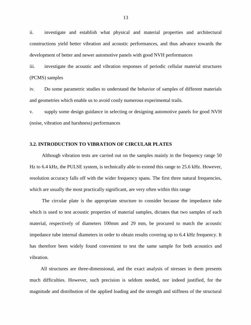
3.2. INTRODUCTION TO VIBRATION OF CIRCULAR PLATES
Although vibration tests are carried out on the samples mainly in the frequency range 50
Hz to 6.4 kHz, the PULSE system, is technically able to extend this range to 25.6 kHz. However,
resolution accuracy falls off with the wider frequency spans. The first three natural frequencies,
which are usually the most practically significant, are very often within this range
The circular plate is the appropriate structure to consider because the impedance tube
which is used to test acoustic properties of material samples, dictates that two samples of each
material, respectively of diameters 100mm and 29 mm, be procured to match the acoustic
impedance tube internal diameters in order to obtain results covering up to 6.4 kHz frequency. It
has therefore been widely found convenient to test the same sample for both acoustics and
vibration.
All structures are three-dimensional, and the exact analysis of stresses in them presents
much difficulties. However, such precision is seldom needed, nor indeed justified, for the
magnitude and distribution of the applied loading and the strength and stiffness of the structural

14
material are not known accurately. For this reason it is adequate to analyze certain structures as if
they are one- or two-dimensional. Thus the engineer’s theory of beams is one-dimensional: the
distribution of normal and shearing stresses across any section is assumed to depend only on the
moment and shear at that section. By the same token, a plate, which is characterized by the fact
that its thickness is small compared with its other linear dimensions, may be analyzed in a two-
dimensional manner. The simplest and most widely used plate theory is the classical small-
deflection theory which we will now consider. The classical small-deflection theory of plates,
developed by Lagrange [66], is based on the following assumptions:
(i) Points which lie on a normal to the mid-plane of the undeflected plate lie on a normal
to the mid-plane of the deflected plate.
(ii) The stresses normal to the mid-plane of the plate, arising from the applied loading,
are negligible in comparison with the stresses in the plane of the plate.
(iii) The slope of the deflected plate in any direction is small so that its square may be
neglected in comparison with unity.
(iv) The mid-plane of the plate is a ‘neutral plane’, that is, any mid-plane stresses arising
from the deflection of the plate into a non-developable surface may be ignored.
These assumptions have their counterparts in the engineer’s theory of beams; assumption (i),
for example, corresponds to the dual assumptions in beam theory that ‘plane sections remain
plane’ and ‘deflections due to shear may be neglected’. Possible sources of error arising from
these assumptions are discussed.

15
3.3 GENERAL PLATE VIBRATION
The subject of plate vibrations is treated to various levels of detail in many texts and
papers, e.g. Timoshenko [17]. Following Timoshenko, Consider an element of a vibrating plate
as shown in Figure 3.1.
Figure3.1: Element of vibrating plate [17]
The plate consists of a perfectly elastic, homogeneous, isotropic material that has a
uniform thickness h which is small in comparison with its other dimensions. We take the xy
plane as the middle plane of the plate and assume that with small deflections the lateral sides of
an element, cut out from the plate by planes parallel to the zx and zy planes (see Fig. 3.1) remain
plane, and rotate so as to be normal to the deflected middle surface of the plate. Then the strain
in a thin layer of this element, indicated by the shaded area and distance z from the middle plane
can be obtained from a simple geometrical consideration and will be represented by the
following equation:
2
2xy
wz
x y
(3.1)

16
It is assumed that the deflections are small in comparison to the thickness of the plate, and
the middle plane is considered to be unstretched.
Thus:
2
2y
wz
y
(3.2)
2
2x
wz
x
(3.3)
In which:
ɛx, ɛy are unit elongations in the x and y directions,
γxy is shear deformation in the xy plane,
w is deflection of the plate,
h is the thickness of the plate.
z is the distance from the shaded area to the middle surface
The corresponding stresses will therefore be obtained from the well-established equations:
2 2
2 2 2
2 2
2 2 2
2
1
1
,1
x
y
xy
Ez w wv
v x y
Ez w wv
v y x
Ez w
v x y
(3.4)
In which ν represents the Poisson’s ratio.
The potential energy stored in the shaded part of the element in the diagram during
deformation will be:
2 2 2
y y xy xyx xdU dx dy dz
(3.5)

17
When the above equations (3.1-3.4) for unit elongations, shear deformations, and stresses are
applied, we have:
2 22 2 2 2 2
2 2 2 22
22
22 1
2 1 ,
Ez w w w wdU v
x y x yv
wv dx dy dz
x y
(3.6)
From this, upon integration, we get the potential energy of bending of the plate as:
2 2 2
2 2 2 2 2
2 2 2 22 2 1
2
D w w w w wU v v dx dy
x y x y x y
(3.7)
Where the flexural (i.e. bending) rigidity of the plate has been denoted by (D), and is given by:
3
212 1
E hD
(3.8)
Where, E is Young’s modulus, h is plate thickness, and ν is Poisson’s ratio.
Similarly, the kinetic energy (T) of the vibrating plate may be written as:
2
2
hT w dxdy
(3.9)
Where ρh is the mass per unit area of the plate, and w is the first derivative of displacement.
From the expressions for potential and kinetic energies, different suitable methods, such as the
energy conservation principle, may be utilized to obtain the natural frequencies
Lord Rayleigh’s method of deducing natural frequencies of vibrating structures consisted
in equating the maximum kinetic energy, Tmax (occurring in the mean position where deflection
is nil but velocity is maximum) to the maximum potential energy, Umax (which occurs in the

18
extreme position where deflection is maximum but the velocity is zero). Ritz introduced the use
of functions to approximate the deflection.
For example, when Ritz studied the vibration of a completely free square plate, he took the
deflection function as:
(3.10)
Where Z is a function of x and y and it determines the mode of vibration, if we take Z in a series
form, we get:
1 1 2 2 3 3, , ,Z a x y a x y a x y (3.11)
Or, in separable form:
mn m n
m n
Z a X x Y y (3.12)
where Xm(x) and Yn(y) are the normal functions of the vibration of a prismatic bar with free ends.
Substituting equation (3.10) into equations (3.7) and (3.9), we get the following expression for
maximum potential energy:
2 2 2
2 2 2 2 2
2 2 2 22 2 1
2
D Z Z Z Z ZU v v dx dy
x y x y x y
(3.13)
The kinetic energy for the plate is given by:
2 2
max2
hT Z dx dy
(3.14)
Where ω, is the natural frequency in Hz.
By equating the maximum potential and kinetic energies, we obtain the eigenvalues (squares of
frequency) of the system
19
2 max
2
2 U
h Z dx dy
(3.15)
The frequencies of vibration are then determined by the equation
2
D
a h
(3.16)
Where α is a constant depending on the vibration mode, ρ is the density, a is the length of the
square rib, and h is the plate thickness. The values for α [17] are (14.1, 20.56, and 23.91) for the
first three modes respectively.
From this equation, some general conclusions can be drawn which hold also in other cases of
vibration of plates, namely,
(a) The period of the vibration of any natural mode varies with the square of the linear
dimensions, provided the thickness remains the same;
(b) If all the dimensions of a plate, including the thickness, are increased in the same
proportion, the period increases with the linear dimensions;
(c) The period varies inversely with the square root of the modulus of elasticity and directly
as the square root of the density of material.
3.4 VIBRATION OF A CIRCULAR PLATE
The above general procedure and results can be easily adapted for circular plates.
Kirchhoff [13] solved the problem of the vibration of a circular plate and calculated the
frequencies of several modes of vibration for a plate with free boundary. The exact solution of
this problem involves the use of Bessel functions. In the following, an approximate solution
using the Rayleigh-Ritz method is used. The Rayleigh-Ritz approach usually gives results of

20
sufficient accuracy for practical applications, when sufficient numbers of terms are retained in
the representing deflection expression. For circular and cylindrical geometries, it is necessary to
transform the energy expressions to polar coordinates.
The basics of this transformation can be seen in figure 3.2. From the elemental triangle
mns it may be seen that a small increase dx would lead to small increases
cosdr dx sin
;dx
dr
(3.17)
Figure 3.2: Model of deformed coordinates in plate vibration [17]
By considering the deflection v as a function of r and ϴ we obtain:
sin
cosw w r w w w
x r x x r r
(3.18)
Similarly we will find:
cos
sinw w w
y r r
(3.19)
Differentiating (3.18) and (3.19) once more we get:
2
2
sin sincos cos
w w w
x r r r r
(3.20)

21
2 2 22
2
2 2
2 2 2
sin cos sincos 2
sin cos sin2
w w w
r r r r r
w w
r r
(3.21)
and
2 2 2 22
2 2
2 2
2 2 2
sin cos cossin 2
sin cos cos2
w w w w
y r r r r r
w w
r r
(3.22)
2 2 2
2 2
2
2 2
cos 2 cos 2sin cos
sin cos sin cos
w w w w
x y r r r r
w w
r r r
(3.23)
These lead to:
2 2 2 2
2 2 2 2 2
1 1w w w w w
x y r r r r
(3.24)
and:
2 22 2 2 2 2
2 2 2 2 2
1 1 1w w w w w w w
x y x y r r r r r r
(3.25)
Substituting (3.24) and (3.25) in equation (3.7) and referencing the plate center as origin then
yields:
22 2 2 2
2 2 2 2
0 0
22
2 2
1 1 12 1
2
1 12 1 ,
RD w w w w w
U vr r r r r r r
w wv rd dr
r r r
(3.26)
Where R represents the radius of the plate.
If the plate deflection is symmetrical about the center, w will be a function of r only, and
the last equation simplifies to:

22
2
2 2
2 2
0
1 12 1
rd w dw d w dw
U D v rdrdr r dr dr r dr
(3.27)
The kinetic energy in polar coordinates is given by:
2
2
0 02
Rh
T w r dr d
(3.28)
and for symmetrical cases,
2
0
R
T h w r dr (3.29)
When these expressions are utilized for the potential and kinetic energies, the frequencies and
natural modes of vibration of circular plates for various particular boundary conditions may be
obtained. In the application of the Rayleigh-Ritz method here we may assume that the solution
takes the form of equation (3.10), however, when Z is expressed as a function of both r and ϴ.
For vibration which is symmetric about the center, Z will be a function of r only, and can be
expressed as:
2 32 2
1 22 21 1
r rZ a a
R R
(3.30)
To get an approximation to the first mode one uses the first term in the representative expansion.
The first two terms are utilized to solve for the second mode, etc. The vibration frequency in all
cases can be determined by the equation shown below [17]:
2
D
R h
(3.31)
Where R is the radius of the plate, ρ is the density, h is the plate thickness, α is called modal
constant, and D is the modulus of rigidity. For a free circular plate with n nodal diameters and s
nodal circles, the values of α are given for various modes in the following table [17].

23
Table 3.1: Alpha values for different nodal lines and circles
s n
0 1 2 3
0 …………. …………… 5.251 12.23
1 9.076 20.52 35.24 52.91
2 38.52 59.86 …….. ………..
3.5 ACOUSTICS THEORY
The acoustics theory of waves incident on plates has also been treated by many authors in
books and technical papers; we have followed the development by Zwikker and Kosten [46],
Biot [67] and Allard [68].
3.5.1 DYNAMICS OF ACOUSTIC PLANE WAVES
In one-dimensional flow, the instantaneous pressure of a sound wave at a point traveling in the
positive coordinate direction may be expressed in terms of frequency, sound speed, coordinate
and time as:
expx
p x A j t xc
(3.32)
Here, j2 is -1, ω is radian frequency equal 2 π . Hertzian frequency in cycles/sec, and A is a
constant. At the starting point x = 0, p(0) = A exp jωt.
If we use the representations β for ω/c, and γ for α + jβ, then:
0 exp .p x p x (3.33)

24
Where γ, called the propagation constant, is a characteristic of the medium. The real and
imaginary parts of this quantity, respectively α and β, are called the attenuation constant and
phase constant. The velocity at a coordinate point can also be written as
0 exp .v x v x (3.34)
The ratio, at a point, of acoustic pressure to acoustic velocity, p(x)/v(x), is called the specific
acoustic impedance, z(x).
In an infinite medium, this impedance depends only on the material of the medium, hence it is
often known as the wave impedance in the medium, W. For an inlet pressure p(0) applied at x =
0 to an infinite medium, instantaneous pressure and velocity at any coordinate may be obtained
from W and γ, which thus completely characterize the acoustic response of such a medium.
3.5.2 ACOUSTIC TRANSMISSION IN THICK FINITE MEDIUM
Let the impedance of a plate having thickness l be z1 at x = 0 and z2 at x = l. Since some of the
sound signal will be reflected back at the termination point x = l, then pressure p at any
coordinate x between inlet and end must be a superposition of both the forward-traveling
(positive) and reflected (negative-traveling) signals:
exp expi rp x p l x p l x (3.35)
and velocity,
exp expi rp pv x l x l x
W W
(3.36)

25
Where pi and pr stand for inward and reflected pressure. The negative sign is necessary for the
velocity of the reflected signal (velocity is a vector) . Using boundary conditions at l as p(l)/v(l)
= z2 in Equation (3.36), we get:
2
2
r
i
z Wp
p Wz
(3.37)
Equation (3.37) and its predecessor taken together yield the impedance z1 at x = 0 as
21
2
cosh sinh
sinh cosh
l W l
l
zz
zW
l W
(3.38)
A particular instance of this relationship occurs when the absorbent is backed by a rigid
termination, thus making the impedance z2 to become infinite, and then
1 coth .z W l (3.39)
3.5.3. ANALYSIS FOR AIR PROPAGATION CONSTANT, γ, AND WAVE
IMPEDANCE, W.
Newton’s second law, or the motion Equation for a layer of air having thickness dx, becomes
0
p v
x t
(3.40)
Where ρo represents air density. The continuity may be stated as
0 0
1 1v d p
x t dp t
(3.41)

26
Let the air bulk modulus, which equals volumetric stress divided by volumetric strain, be
represented by K0= dp/ ((dρ/ρ0)). Eliminating v by equating the signed differentials of equation
(3.40) with respect to x and equation (3.41) with respect to t respectively leads to:
2 2
0
2 2
0
.p p
x K t
(3.42)
But pressure p along coordinate x can be defined in terms of frequency, time, and propagation
constant as:
0exp expp A j t x (3.43)
Equation (3.43) may be substituted into (3.42) to obtain:
2 200
0K
(3.44)
Then:
00
0
jK
(3.45)
A comparison of equations (3.32) and (3.45) leads to the physical meaning of √ (ρ0/K0 ) as the
velocity, co of sound propagation in air. When equation (3.45) and the velocity expression
0exp expv B j t x (3.46)
Are substituted into the wave impedance equations (3.40) and (3.41), we obtain
0 0 0 0 0
pW K c
v (3.47)

27
3.5.4 DEDUCTION OF ABSORPTION AND REFLECTION COEFFICIENTS
Consider the plane waves through the air to be incident at a wall of specific impedance z. The
reflection coefficient, r, thus becomes:
0
0
r
i
z Wpr
p z W
(3.48)
This is based on pressure. Hence, based on energy, which is proportional to (pressure) 2, R = |r|
2,
where R is the energy-based reflection coefficient. Assuming that the sound is only either
absorbed or reflected, α + R add up to unity, where α is the energy-based absorption coefficient,
thus:
22
00
0
1 1r
i
z Wp
p z W
(3.49)
Here, according to equation (3.49), Wo can be replaced by ρoco, the product of air density and
sound velocity in air. Equation (3.49) can then be rendered as:
2
0 00
0 0
1
1
1
z
c
z
c
(3.50)
Recalling that z/ρoco is a complex quantity with a real and an imaginary part, then:
0 0
0 2 2
0 0 0 0
4Re
Re 1 Im
z
c
z z
c c
(3.51)

28
3.5.5 ACOUSTIC ANALYSIS OF RIGID POROUS MATERIALS
Acoustic absorption is normally attributed to heat generation and dissipation, and also dissipative
viscous friction. Increased surface area from surface extension, roughness, pores and more
tortuous paths enhance these effects. The Rayleigh model of acoustic propagation is one that
simplifies the rigid porous medium as comprising multiple parallel air channels within a similar
rigid frame. Using a low-frequency approximation that ignores air inertia and focusing on one
cell. Flow resistance (R), defined per unit length of this cell, as pressure gradient divided by
average velocity, is given by
1 p
Rv x
(3.52)
Where v is average velocity. In a medium of viscosity η and a narrow channel of width b,
2
12R
b
(3.53)
But for a circular section cell of radius a,
2
8
*R
d a
(3.54)
Where d is the material thickness.The flow per unit cross section area per unit time is defined as
the Rayl, and the unit of the specific flow resistance is Rayl per cm of cell length traversed. For
an element length dx, equating the internal motive force (Mass. acceleration) in the positive
direction to the sum of external forces, i.e. net pressure force and flow resistance in the same
direction yields ρodxda. v / t = - p/ x. dxda – R v dxda, where cross section area is a, gives
0 2
1v p
x t c t
(3.55)

29
When some flow channel areas are unparallel to sound-impacted material surface a constant
called the structure factor, Ks, is introduced. It is defined as the ratio of the unparallel plus
parallel channel area to the parallel, and may be used to multiply the medium density to yield an
effective density ρs. If porosity, Ω, defined as the ratio of total void area to overall area. The
motion and continuity equations become
0
P vRv
x t
(3.56)
2
0
p v
c t x
(3.57)
The pressure and velocity equations in the case of a harmonic plane wave then become
ˆ expP P j t x ,
ˆexpv v j t x (3.58)
Merging the last equations set into the preceding equation gives the equations
0ˆ ˆ 0j P j R v
, 2
0 0
ˆ ˆ 0j
P j vc
(3.59)
r, setting the coefficients of the amplitude expressions P and V to null,
0
2
0 0
0
j j R
jj
c
(3.60)
11 22
2
0 0
s
RK i
c
(3.61)
From the earlier definition, the wave impedance becomes

30
1
20 0
1
02
s
cp RW K i
v
(3.62)
The two equations (3.61) and (3.62) may be applied with the appropriate boundary conditions for
the solution to many propagation problems. An example is when the medium is a rigid porous
material, and the boundary is a rigid wall termination, in which the surface impedance z is now
obtained from these two equations substituted back into (3.38) as
111 22
0 0 21
0 02
coths s
c R Rz K i j K j d
c
(3.63)
Where d is the material thickness, and the acoustic absorption coefficient α can then be obtained
by inserting the last equation (3.63) into (3.49).

31
CHAPTER 4
EXPERIMENTAL WORK
4.1. MATERIALS
In such a work as this, it is although experiments will be augmented by parametric studies,
it is essential that a reasonable number of types of materials be tested, so that results pertaining to
a broad class of materials may be obtained for better generality of conclusions. For this purpose,
a variety of materials, both traditional (for comparisons) and novel, are classifiable into six
groups, were tested. They include fabric materials, foam materials, honeycomb materials,
monolithic and sandwich materials, periodic cellular material structures, and generally periodic
materials. The materials have been chosen, either for their economic importance in the vibro-
acoustic industry or for their novelty and promise in the area. Tested fabric materials included
basalt, resonated cotton, two types of fiberglass, and polyethylene terephthalate (PET) fiber
mass. Two foam materials under development for acoustic containment were supplied by the
Kathawate Inc. Company, and respectively named Kathawate magic foam orange, and
Kathawate magic foam white. These were expanded in our laboratory oven at 150 degree Celsius
from plastic feedstock. In addition polyurethane foam from the Bruel & Kjaer Company was
also tested. Seven honeycomb materials of different material or structural characteristics were
tested. These were the all-aluminum honeycomb, fiberglass/Nomex honeycomb; cold rolled steel
(CRS)/Nomex honeycomb, glass-epoxy/aluminum honeycomb, glass-epoxy/polypropylene (PP)
honeycomb.AA5.2-95, epoxy-primed aluminum/aluminum honeycomb.AA3.6-80, and phenolic
coated polyester/Aramid (Nomex) core honeycomb. The class of monolithic and sandwich
constructions included the Lexan, and cold-rolled steel monolithic as well as CRS//hard foam
32
and steel/polypropylene (USIL Light) sandwiches. Three periodic cellular material structure
(PCMS) materials from Cellular Materials International (CMI) Inc. were also tested. The
rationale for choosing this group of materials is that they are novel, multifunctional, and have not
been tested for vibro-acoustic applications yet. Applications to heat transfer, conduit, structural,
and other applications have been explored and adopted. The materials are the aluminum
prismatic Microtruss, the aluminum pyramidal Microtruss, and the stainless steel triangular
honeycomb PCMS. The general periodic materials tested were the single row Micropillars with
resonators, the double row, in-line Micropillars, and the double row, staggered Micropillars.
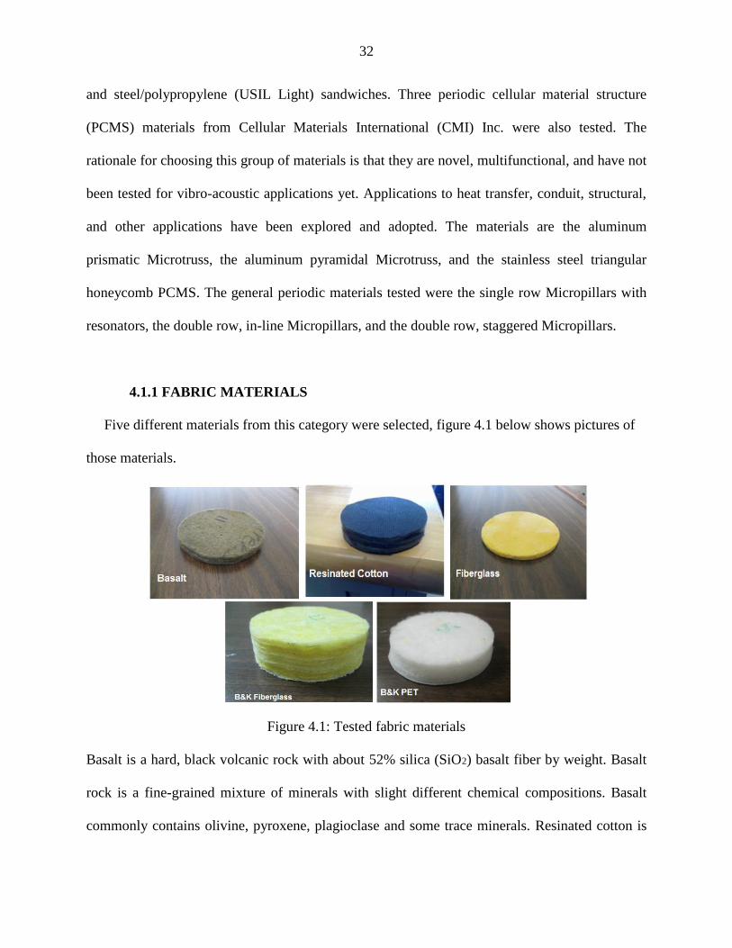
4.1.1 FABRIC MATERIALS
Five different materials from this category were selected, figure 4.1 below shows pictures of
those materials.
Figure 4.1: Tested fabric materials
Basalt is a hard, black volcanic rock with about 52% silica (SiO2) basalt fiber by weight. Basalt
rock is a fine-grained mixture of minerals with slight different chemical compositions. Basalt
commonly contains olivine, pyroxene, plagioclase and some trace minerals. Resinated cotton is

33
bonded acoustical cotton, with panels normally available in 3 lb. or 6 lb. per cubic foot densities,
and various area sizes. They are both flame and noise resistant. Fiberglass is used as for acoustic
absorption, considered effective, especially at high densities and thicknesses from 2 inches
upward. The geometrical properties of the samples tested are shown in table4.1 below, taking
into account that all the samples are 100mm diameter. Polyethylene terephthalate plastic fibers
have been found to be one of the better plastic materials to deploy in automotive acoustic
abatement.
Table 4.1: Fabric materials properties
Material Weight(gram) Thickness(mm) Density(kg/m3)
Basalt 15.7 12.7 157
Resinated cotton 24.68 17 184.84
Fiberglass 4.05 9.5 54.36
B&K Fiberglass 22.35 27 105.4
B&K PET 3.91 18 27.65
4.1.2 FOAM MATERIALS
The foam material, by its unevenness and porosity, naturally yields much larger effective
areas (some products claim about 400% and upwards) for sound mitigation than plain, smooth
surfaces, and also permits sound signals to sink to various depths. Soft polyurethane is well
known to generally control noise propagation. The two proprietary foams tested came from the
G. R. Kathawate Inc. company, and are being developed for sound control, based, according to
them, on the construction of the surface properties of the materials, figure 4.2 and table 4.2
below shows pictures and geometrical properties of the samples tested respectively.
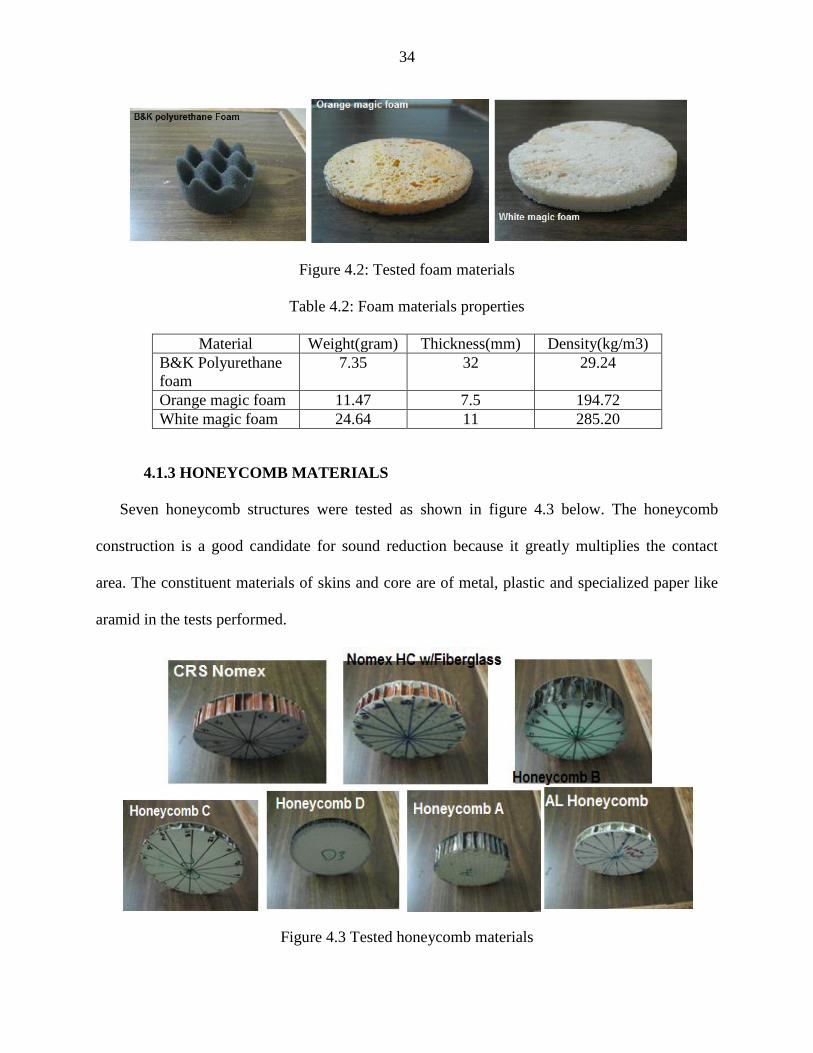
34
Figure 4.2: Tested foam materials
Table 4.2: Foam materials properties
Material Weight(gram) Thickness(mm) Density(kg/m3)
B&K Polyurethane
foam
7.35 32 29.24
Orange magic foam 11.47 7.5 194.72
White magic foam 24.64 11 285.20
4.1.3 HONEYCOMB MATERIALS
Seven honeycomb structures were tested as shown in figure 4.3 below. The honeycomb
construction is a good candidate for sound reduction because it greatly multiplies the contact
area. The constituent materials of skins and core are of metal, plastic and specialized paper like
aramid in the tests performed.
Figure 4.3 Tested honeycomb materials

35
Table 4.3 below shows the properties of honeycomb materials, the Young’s modulus, and
Poisson’s ratio have been gotten through curve fit approach, the values showed good match
between experimental and finite element simulation. For those cases where no property value
was available, the curve fit approach consisted in interpolating trail values until a mach with
experiment was achieved. This was done using the finite element method. We resorted to this
approach after failing to obtain these values from exhaustive literature search, coupled with
persistent and diligent inquires from several companies.
Table 4.3: Properties for Honey comb Materials
# Panel ID Skin Core Cell
Size(inch)
Weight
(gram)
Total Density
(kg/m3)
Young’s Modulus
(Mpa)
Poisson’s
ratio
1 AA5.2-95
(A)
Glass epoxy
t=0.018”
Aluminum
Honeycomb
ρ=5.2pcf
1/4 28.34 48 2438 0.4
2 PP5.0-90
(B)
Glass epoxy w/peel
ply t=0.014”
Polypropylen
e
Honeycomb,
ρ=5 pcf
1/4 29.5 47 1100 0.28
3 AA3.6-80
(C)
Aluminum epoxy
primer
finish(t=0.02”)
Aluminum
Honeycomb,
ρ=3.6pcf
3/8 26.1 140 2100 0.35
4 PN1-1/8-
3.0
(D)
Polyester Aramid
Nomex
1/8 17.5 89.5 2250 0.25
5 Aluminum
(0.032”,0.02”)
Aluminum 3/8 40.8 130.65 2000 0.4
6 303 Fiberglass
(0.01”)
Nomex
Honeycomb
1/4 21 52.86 1800 0.37
7
*
- CRS(0.024”) Nomex
Honeycomb
- 79.25 179.76 - -
*: this material was not simulated using Finite element according to the thickness of the core.
4.1.4 MONOLITHIC AND SANDWICH MATERIALS
This group encompasses the cold rolled steel (CRS), Lexan (a polycarbonate plastic) as
monolithic materials, where, CRS with LE5208 foam, and USIL light (trade name) which is a
steel skins and thin polypropylene core are the sandwich materials (figure 4.4).

36
The Lexan material was tested in many structural forms, including simple solid, multi-layer
solids, disks with holes of different sizes, and layered structures of some combinations of these.
Figure 4.4: Tested monolithic and sandwich materials
Table 4.4 shows the properties of those materials.
Table 4.4: Properties of sandwich and monolithic materials
Material Density
(kg/m3)
Young’s
Modulus(Pa)
Poisson’s
ratio
Thickness
(mm)
Mass(gram)
Skin core Skin core Skin core Skin core
CRS
w/LE5208
7870 800 205e9 1.35e9 0.29 0.27 0.75 5 128
USIL Light 7870 1990 205e9 12.85e9 0.29 0.26 0.375 0.75 38.2
Lexan 1200 2350e9 0.375 2.2 21

37
4.1.5 PERIODIC CELLULAR MATERIAL STRUCTURES (PCMS) MATERIALS
PCMS are multifunctional materials often used as cores of general honeycomb structures.
They are usually made of struts (tetrahedral, pyramidal, etc), prismatic (triangular, square,
hexagonal, etc.), and shell (egg-case, etc.) types of elements. The three types tested are shown in
Figure .they have great functional and economic importance and have started to be utilized by
the military (ONR/US Navy) and industrial interests. Their multi functional uses have been
applied for heat exchanger constructions [69][70]. Figure 4.5, and table 4.5 below shows those
materials and their properties respectively.
Figure 4.5: Tested periodic cellular material structures (PCMS) materials
Table 4.5: Properties of PCMS materials
Material Density(kg/m3) Young’s
Modulus(Pa)
Poisson’s ratio
PCMS Aluminum 2700 68.9e9 0.33
PCMS Stainless Steel 800 200e9 0.29
4.1.6 GENERAL PERIODIC MATERIALS
There is an almost infinite number of ways to construct these structures, which basically
manifest regular periodicity in their arrangement. This confers on them some response behaviors
in case of mechanical, acoustic, and various other types of excitations. We tested three micro-

38
pillars structures in this category, and they are shown in figure 4.6 below. Although this research
doesn’t include analysis of the vibroacoustics of meta materials ,this work gives experimental
results for these constructions which constitute candidate meta materials .If we can tune the
masses and springs appropertly we should get the negative effective mass , effective stiffness
and band gaps which normally characterize meta materials ,this aspect is being reserved for a
future research. The micropillars are made of nylon 66 cylinders, and the metal parts are of mild
steel, including the masses (nuts) of the internal mechanical resonators in the first case. The
properties of these materials are shown in table 4.6 below.
Figure 4.6: Tested general periodic material structures
Table 4.6: Properties of general periodic material structures
Material Young’s
Modulus(Mpa)
Density(kg/m3)
Thickness of
skin(mm)
Poisson’s Ratio
Nylon 66 811 645 Dia(2.5) 0.4
Mild Steel 210000 7880 Dia(4) 0.3
Aluminum
6061T
68900 2700 1.54(sample1)
0.43(sample 2
and 3)
0.33
4.2 APPARATUS
In both cases of vibration and acoustics testing, the core of the system was the
computerized “PULSE” vibration and acoustics hardware and software system, made by Bruel &

39
Kjaer Company [71]. It’s most recent software PULSE 16.0 was utilized. Later the PULSE
Reflex 16.1 was adopted as it became available from B&K.
4.2.1 VIBRATION TEST APPARATUS
The vibration test apparatus consists of the PULSE front end which contains the channels
that connect the cables for both the force and acceleration transducers, the accelerometers and
hammers used in the experiments were from Bruel& Kjear Inc., and PCB Piezotronics Inc, the
range of those accelerometers is from 0 up to 50 kHz to cover complex structures that have high
natural frequencies, those accelerometers were calibrated according to the manufacturer
recommendations, the front end is connected to the computer through an ether net cable and it
has its own IP address, the PULSE software was installed on the computer for post processing
the data collected from each experiment. All these components are shown in figure 4.7 below
Figure 4.7: Vibration test apparatus with its components
A sketch is shown in figure 4.8 below to demonstrate the different components and how they are
connected together, the geometry which we draw inside the software to indicate a circular disk
with the transducers on it is shown in figure 4.9 below, the hammer is shown at each point to

40
indicate that the experiment was done with a roving hammer at each point while the
accelerometer is fixed at a specific point.
Figure 4.8: A sketch for the vibration apparatus
Figure 4.9: Geometry drawn inside PULSE, the hammer is roving, while accelerometer is fixed
at point1.
4.2.2 ACOUSTICS TEST APPARATUS
The acoustics apparatus contains the PULSE front end and the computer for the data
processing, as mentioned before for the vibration apparatus, however the acoustics one includes
the impedance tube in which the sample is fixed inside ,this tube has two types, the large one
which is shown in figure 4.10 below, this is 100mm diameter and is used to calculate the sound
absorption in the low frequency range(0-1.6 kHz), the other part is the small tube which is used

41
to measure the sound absorption in the high frequency range(500 Hz-6.4 kHz), the other part of
this apparatus is the power amplifier which is used to generate a sound signal inside the tube
,also it contains knobs to calibrate the gain and the current levels .
Figure 4.10: Acoustic test apparatus
To demonstrate the impedance tube from inside, figure 4.11 shows a cutaway of this
tube, it is clear that there is an incident acoustic wave and a reflected acoustic wave, the software
is capable of calculating the sound absorption coefficient according to these values as it will be
shown later.
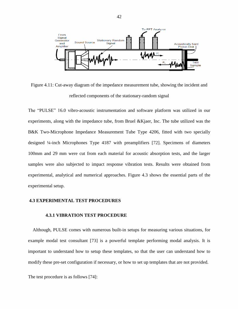
42
Figure 4.11: Cut-away diagram of the impedance measurement tube, showing the incident and
reflected components of the stationary-random signal
The “PULSE” 16.0 vibro-acoustic instrumentation and software platform was utilized in our
experiments, along with the impedance tube, from Bruel &Kjaer, Inc. The tube utilized was the
B&K Two-Microphone Impedance Measurement Tube Type 4206, fitted with two specially
designed ¼-inch Microphones Type 4187 with preamplifiers [72]. Specimens of diameters
100mm and 29 mm were cut from each material for acoustic absorption tests, and the larger
samples were also subjected to impact response vibration tests. Results were obtained from
experimental, analytical and numerical approaches. Figure 4.3 shows the essential parts of the
experimental setup.
4.3 EXPERIMENTAL TEST PROCEDURES
4.3.1 VIBRATION TEST PROCEDURE
Although, PULSE comes with numerous built-in setups for measuring various situations, for
example modal test consultant [73] is a powerful template performing modal analysis. It is
important to understand how to setup these templates, so that the user can understand how to
modify these pre-set configuration if necessary, or how to set up templates that are not provided.
The test procedure is as follows [74]:
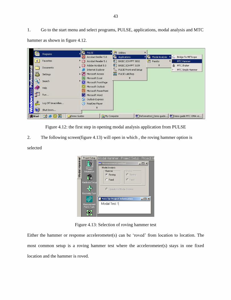
43
1. Go to the start menu and select programs, PULSE, applications, modal analysis and MTC
hammer as shown in figure 4.12.
Figure 4.12: the first step in opening modal analysis application from PULSE
2. The following screen(figure 4.13) will open in which , the roving hammer option is
selected
Figure 4.13: Selection of roving hammer test
Either the hammer or response accelerometer(s) can be ‘roved’ from location to location. The
most common setup is a roving hammer test where the accelerometer(s) stays in one fixed
location and the hammer is roved.

44
3. PULSE automatically detects whether or not the connected data acquisition equipment
matches the saved configuration. If the hardware is different, PULSE prompts the user to
reconfigure.
4. When you click the hardware setup window, detect TEDS (transducer electronic data
base) appears, as shown in figure 4.14, which checks for and automatically configures TEDS
transducers on all channels but keeps the existing setup for channels with non-TEDS transducers.
It is important to mention here that most force sensors and impact hammers do not have TEDS;
in this case any non-TEDS channels are cleared and must be manually reconfigured. To do this,
in the configuration tab, we add any non-TED transducer to the system by inputting the data
related to this transducer like sensitivity, weight, serial number, and then saving it in the
database.
Figure 4.14: Detection of Transducer electronic database
5. In the geometry window we insert the dimensions of the geometry we want to test, then
insert the number of points we want to hit, in our case we plot a circle with 17 points, then we
should assign a transducer for each point, In this case each point gets one hammer hit, The
transducer (accelerometer) is located at point 1.
6. In the measurement sequence task, a complete measurement plan is found. For each
measurement, both excitation and response point and direction are indicated. The sequence is
editable by the changing point numbers for a measurement, as was shown in figure 4.9 before.

45
7. In the analyzer setup task, select the number of impacts that will be made at each location
by setting the number of averages in the modal FFT (fast Fourier transform) analyzer window.
Set the averaging mode to linear.
8. In the hammer setup task, choose the trigger level setup in the hammer view as shown in
figure 4.15. Press the activate button, and wait for the system to activate.
Figure 4.15: Trigger level setup selection
Then, press the start button, to start the hammer recorder. Impact the structure several times with
the same force level to be used during the test as shown below. The trigger level can be
graphically set by moving the blue line up or down as shown in figure 4.16 below.
Figure 4.16: Setting the trigger level manually

46
9. In the response setup task, press the activate button, and wait for the system to activate. Press
the start button. Impact the structure with the same force level to be used during the test. The
response window can be graphically set in the response view. A uniform window is the
preference for impact testing since it does not affect damping like an exponential window, as
shown in figure 4.17.
Figure 4.17: Response window shows the signal decay with time
10. In the measurement task, press the activate button, and wait for the system to activate.
When a measurement is selected in the measurement control window, the geometry window
shows where to place the accelerometer(s) for that measurement. Press the start button, to start
the generator and analyzer. The average monitor indicates the number of averages during the
measurement. When the measurement is finished, press the Save button to proceed to the next
measurement. Click on the measurement number in the measurement to view results from
47
different measurement. Measurement can be taken by selecting the measurement tab, pressing
start and then save.
4.3.2 PULSE REFLEX™ MODAL ANALYSIS
PULSE Reflex is the latest addition to the PULSE platform of software products by
Brüel&Kjær [75]. It provides post-processing in a modern, intuitive GUI (graphical user
interface) environment and it resolves the most important issues when analyzing sound and
vibration data.
PULSE reflex modal analysis is an efficient workflow with just a few steps to perform a
complete
Modal analysis, i.e., modal analysis based on hammer and shaker testing. It allows the user to
observe, analyze and document the dynamic behavior of structures and provides accurate and
reliable results.
It is an easy-to-use post-processing application that enables the user to perform Classical Modal
Analysis even in the most demanding situations by using a set of best-in-class mode indicator
functions, curve-fitters and validation tools. Accurate results are quickly obtained by following
an intuitive and flexible workflow process that guides the user efficiently through measurement
validation, parameter estimation setup, mode selection, analysis validation and reporting.
The steps included in PULSE Reflex Modal Analysis are [75]:
1. Geometry creation and import
Geometry can be imported in standard data formats like UFF, DXF and CSV from PULSE
hammer test; alternatively, geometries can be created from scratch using the embedded drawing
tools. The measurement DOFs (degrees of freedom) contained in the imported measurement files

48
are automatically added to and shown on the geometry in the subsequent tasks as shown in figure
4.18.
Figure 4:18: Geometry imported from PULSE to Reflex
2. Measurement validation
The Measurement validation task is used to check the quality of the measurement data prior to
performing the modal parameter extraction. Functions like Coherence, FRF (frequency response
function), from selected references can easily be shown by simply dragging the functions from
the Project Browser.
The Geometry Driven Function Display provides a graphical tool that allows the user to select on
the geometry the DOFs that are to be used for the displayed function types. Figure 4.19 shows
the measurement validation step
Figure 4.19: Measurement validation step in Reflex
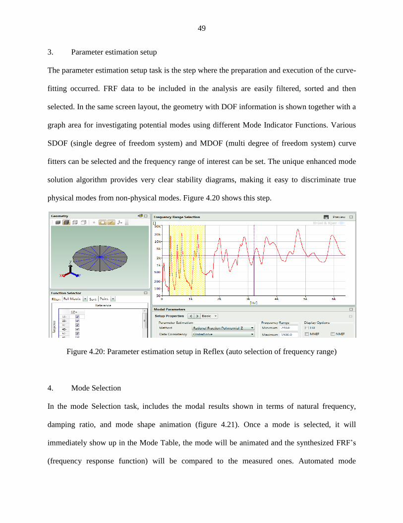
49
3. Parameter estimation setup
The parameter estimation setup task is the step where the preparation and execution of the curve-
fitting occurred. FRF data to be included in the analysis are easily filtered, sorted and then
selected. In the same screen layout, the geometry with DOF information is shown together with a
graph area for investigating potential modes using different Mode Indicator Functions. Various
SDOF (single degree of freedom system) and MDOF (multi degree of freedom system) curve
fitters can be selected and the frequency range of interest can be set. The unique enhanced mode
solution algorithm provides very clear stability diagrams, making it easy to discriminate true
physical modes from non-physical modes. Figure 4.20 shows this step.
Figure 4.20: Parameter estimation setup in Reflex (auto selection of frequency range)
4. Mode Selection
In the mode Selection task, includes the modal results shown in terms of natural frequency,
damping ratio, and mode shape animation (figure 4.21). Once a mode is selected, it will
immediately show up in the Mode Table, the mode will be animated and the synthesized FRF’s
(frequency response function) will be compared to the measured ones. Automated mode

50
selection is supported for fast preliminary investigations of unknown structures or when
conducting repetitive testing. It also eliminates the potential risk of user-dependent results.
Automated mode selection works for all MDOF curve-fitters by indicating the modes in the
stability diagrams, populating the mode table, animating the first mode and showing the
synthesis functions. The Mode Selection task provides full flexibility for selection and
comparison of modes from different curve fitting.
Figure 4.21: Mode selection in Reflex (natural frequencies and mode shapes)
5. Analysis validation
The analysis validation task (figure 4.22) supplies the user with a number of tools for further
investigation of the obtained modal results for maximum confidence in the obtained modal
model like Mode Shapes Animation, and AutoMAC (modal assurance criterion) tables.

51
Figure 4.22: Analysis validation includes the first two modes.
6. Reporting
The report task enables reports to be prepared in parallel with the analysis process, linking
important results as they are produced. Store geometries, displays, tables and text in the project
browser as report elements so when you are ready, you only need to generate and save the report.
Reports are easily created directly in Microsoft word, Excel or PowerPoint.
. 4.3.3 ACOUSTICS TEST PROCEDURE
The two-microphone acoustic impedance measurement tube type 4206[72] is used in
measuring the acoustic absorption coefficient, acoustic reflection coefficient and normalized
impedance there are many others but we are mainly interested in the acoustic absorption
coefficient although the resolution gets poor with the higher frequencies and frequency
bandwidths. It takes quick measurements over a large frequency range. It is software-controlled
and the data is easily manageable. It is used to measure complex or composite materials,
laminates, alloy materials and etc. It can be also used to measure the acoustic properties of the
material that are sensitive to orientations.

52
The two-microphone impedance tube uses two specially designed ¼ inch microphones
with preamplifiers. It has a Bruel and Kjaer dual channel signal analyzer embedded in PULSE.
There are three types of tubes available in two-microphone impedance measurements tube of
type 4206. We use two, one is a large tube, which is also called low-frequency measurement tube
as it measure frequency ranging from 50 Hz to 1.6 kHz. It has three couplers for mounting
microphones flush with the inside of the tube. The second is a small tube also called high
frequency measurement tube and its frequency range varies from 500 Hz to 6.4 kHz. It has two
microphone couplers which are mounted directly on to the open end of the large measurement
tube. There is a large and a small sample holder and both have an acoustically hard back-plate,
which is connected to a sliding piston. The types of frequency weighting unit are according to
the type of tube (large/small) used and the accuracy needed for the measurement of the
parameter. They are high-pass, low-pass and the linear pass. High pass is used with small tube
and for high frequency measurements. The linear is used with large tube for low frequency
measurements and for the extra measurement accuracy below 100 Hz the low pass is
recommended.
The sequence for preparation is:
i. Connect amplifier to impedance tube filter using 2 banana plugs
ii. Set noise generator, amplifier, and filter characteristics to specifications desired
iii. Screw microphones onto impedance tube
iv. Connect the microphones to the front end and choose channel 3 to microphone 2 and
channel 4 for microphone 3.
v. Open the PULSE software and choose from applications the acoustic material testing in
tube, then choose the normal incidence absorption.

53
vi. Go to project setup in the PULSE window and choose “connect signals” to insure that the
microphones are connected adequately to the front end.
Procedure followed for the measurement in both large and small tube:
1. Once the setups are done the test is run on the calibration sample and the sensors are
calibrated. At this time we have already got calibration curve for use with both the large and
small tubes and this can be saved in directory and then it can be directly utilized in future
whenever we want to take test on other material samples instead of calibrating the instrument
again.
2. Now place the test sample inside the tube and make sure it is exactly aligned with the
inside of the tube with no air gap between rigid backup plate and the sample holder. If there is an
air gap, remove it by adjusting piston position to and fro.
3. Start the measurement.
4. The analyzer generates a random signal, which is then amplified by power amplifier and
frequency weighted by frequency weighting unit in the tube and then applied to the sound
source. The analyzer then measures the frequency response of the two microphones channels and
calculates H1 frequency response function. From the incident and reflected components of the
sound pressure at the two microphone positions, PULSE calculates the H1 frequency response
functions, Hi frequency response functions associated with incident component and Hr frequency
response functions associated with the reflected component.
5. Read off or save the results.
The PULSE system is able to obtain several parameters including the reflection coefficient,
the absorption coefficient, normalized impedance, frequency response function, and calibration
data each with magnitude, phase, real and imaginary part etc. The post-processing facilities of

54
the PULSE may then be requested to present the results for any of the parameters in various
graphical, data or tabular forms. Data export to Excel may also be utilized to plot results in
several ways.
For example, using frequency response functions, the reflection coefficient R, is calculated
internally in PULSE from the expression.
)(2
12
12 slkj
r
i eHH
HHR
(4.1)
Where k is wave number, s is distance between two microphones and l is distance between the
first microphone and the material sample.
Using value of reflection coefficient, the normalized impedance and acoustic absorption is
also found from the expressions
R
R
c
z
1
1
(4.2)
2
1 R (4.3)
The two-microphone theory assumes plane-wave propagation, no mean flow and no losses due to
absorption at tube wall. For the accuracy of the measurement we can rotate the sample by 90
degree every time and take four different measurement for circular sample and then using the
post processing tools to find the mean curve of all the four curves and the resultant mean curve
will be the most accurate curve of the parameter being measured.
The PULSE software has excellent post processing features like combination of
measurement data in overlapping frequency ranges, simultaneous graphical display of several

55
sets of measurement data, averaging of up to ten sets of measurement data and data file
management on hard or floppy disk and hard copy facilities in tabular or graphical format.
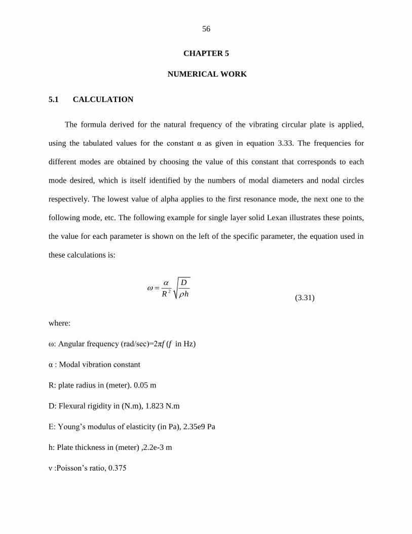
56
CHAPTER 5
NUMERICAL WORK
5.1 CALCULATION
The formula derived for the natural frequency of the vibrating circular plate is applied,
using the tabulated values for the constant α as given in equation 3.33. The frequencies for
different modes are obtained by choosing the value of this constant that corresponds to each
mode desired, which is itself identified by the numbers of modal diameters and nodal circles
respectively. The lowest value of alpha applies to the first resonance mode, the next one to the
following mode, etc. The following example for single layer solid Lexan illustrates these points,
the value for each parameter is shown on the left of the specific parameter, the equation used in
these calculations is:
2
D
R h
(3.31)
where:
ω: Angular frequency (rad/sec)=2πf (f in Hz)
α : Modal vibration constant
R: plate radius in (meter). 0.05 m
D: Flexural rigidity in (N.m), 1.823 N.m
E: Young’s modulus of elasticity (in Pa), 2.35e9 Pa
h: Plate thickness in (meter) ,2.2e-3 m
ν :Poisson’s ratio, 0.375

57
ρ: Material density (kg/m3), 1200 kg/m
3
Table 5.1 shows the first three natural frequencies for single layer solid Lexan.
Table 5.1 Calculated Natural frequencies for Solid Lexan
Mode # α value # of nodal
diameters
# of nodal
circles
Natural
frequencies(Hz)
Mode1 5.252 2 0 f1=320
Mode 2 9.076 0 1 f2=553
Mode 3 12.25 3 0 f3=746
5.2 FINITE ELEMENT
Finite Element Analysis (FEA) is considered as a numerical method to provide solutions to
many engineering problems that couldn’t be solved manually. In 1943 R.Courant used Ritz
method to obtain an approximate solution for some vibration problems [76].
FEA consists of a mathematical model of a material or design that is analyzed for specific
results, in this application the results are the natural frequencies, and mode shape. In finite
element method the structure under study is divided into very tiny elements connected together
by nodes .The preprocessor and post processor were Hypermesh version 10 from Altair
Engineering Inc, the solver used was Abaqus standard 3D. The algorithm used in this solver was
Lancsoz Eigensolver Method to calculate the fundamental frequencies and the corresponding
mode shapes related to each frequency as this method is considered a powerful tool for
extraction of the extreme eigenvalues and the corresponding eigenvectors of vibration problems
in engineering [77]. It uses interpolation methods to extract mode shapes and natural frequencies
for mechanical structures with complex geometries.
The samples are considered as solid. According to the complexity of some structures like PCMS
and Honeycomb, the Unigraphics software was used to draw these geometries, and we then

58
imported them to hypermesh in which the geometry was meshed and the material properties were
plugged inside the software .The element type is really significant in ABAQUS software to
obtain accurate results and it depends upon the mesh style used for each case. The element types
for each case will be shown later on, as an example the C3D20R quadric element type, which is
the second order of the C3D8R quadric element type, is used in some of the simulations. This
element type allows us to increase the integration points on each element and to obtain more
accurate results. The boundary condition which we consider in this simulation is the completely
free boundary conditions. Hypermesh post-processor is used to show the natural frequencies,
displacements, and mode shapes. The results showed a very good agreement between the
experimental results from PULSE Reflex and Abaqus finite element analysis as we will see later.
It should be mentioned here that the license which we have at Wayne State University is limited
to 100000 nodes. On the other hand the thickness of some structures like Nomex was so thin that
the software was not able to mesh it. The second finite element analysis solver used was Radioss
in which the frequency response function was calculated using the fast Fourier transform, the
most important point in this simulation is the capacity of the processor (CPU) of the computers
which we have in our lab, the accuracy of results in this solver depends strongly on the frequency
step length used, the lesser the better. Also the number of nodes selected to show FRF is
important - in this case the more the better. We got some good results that show a match between
experiment and simulation for some materials. However the simulation took around 2 weeks in
some cases where the geometry is heavy.
The selected frequency range was different from case to case depending upon the experimental
results. The maximum value selected was 24 kHz for PCMS materials, and the number of
elements (type PSOLID) used exceeded 450000 in some cases. The material properties, Young’s

59
modulus (E), Poisson’s ratio (ν) and mass density (ρ) were inserted and the geometry with no
constraints (representing completely free boundary conditions in the vibration) were input. The
work was saved, and the solver was then accessed to compile the work and obtain the results. It
should be emphasized here that the material properties for honeycomb samples were difficult to
get either from the company or the literature, so the curve fit approach was used to get
approximate values for these properties. After an interpolation and extrapolation, we succeeded
to get values that showed a reasonable match between experimental and simulation results for
these materials. This approach of reverse engineering may be modified in the future to get even
more accurate results.
The particulars and procedure to calculate vibrations parameters for the plate are
summarized below to calculate the eigenvalues (natural frequencies) and eigenvectors (mode
shapes) for circular plates is:
Pre- and Post-Processor: Hypermesh (Version 10 from Altair Engineering Inc.)
Solver: Abaqus standard 3D, and RADIOSS
Selected frequency range: 0 to 24 kHz
Elements Type: PSOLID
Number of elements: 10000-470000
Mesh Style: It depends upon structure
Solver: Lanczos Eigen Solver (for normal modes)
Procedure:
For the RADIOSS solver[78] which was used to extract the frequency response function (FRF),
for a specific material, again in the preprocessing stage, the geometry was constructed, then the
material properties were assigned for the geometry, the frequency range of interest was chosen, a
specific dynamic load was put on the structure at a specific node and direction. The frequency
resolution (df) is inserted for the purpose of fast Fourier transform (FFT) calculations. It proved

60
difficult to use very small values of this variable because of limited CPU (central processing
unit) capacity. On the other hand a small number of nodes were selected in order to see the FRF
of the structure through them. Increasing the number of selected nodes will show better results as
one or more of these nodes my lie on a nodal line or circle, but there was no ability to increase
this number due to limited processor capabilities. However the results obtained were acceptable.
5.3 MATLAB
The Matlab simulation system was also used to solve the vibration problem, in order to have
assurance of accuracy among several methods. The vibration toolbox was used to insert the
values of the plate radius, thickness, Young’s modulus, and Poisson’s ration. The functions
“Plate_Pars”, and “cirplate” from the command window were used to calculate the plate
frequencies. The function “plotmsh4(m,n) , where m represents the number of nodal diameters
and n the number of nodal diameters and n the number of nodal circles, was used to plot the
mode shape of any specific mode. The function ANIMODE4(m,n) was used to animate any
mode shape desired, The completely free boundary condition was realized by setting “
BC_Spec” (an integer specifying the boundary condition) to zero..
The Handbook “Stress, strain and structural dynamics” [79] was utilized in writing the
Matlab computer program to calculate the natural frequencies of the circular plates and animate
their mode shapes. Appendix B contains the code for calculating these modal values for solid
Lexan. A stepwise procedure is:
Vibration toolbox: used to insert the values of the plate radius, thickness, Young’s
modulus, and Poisson’s ration).

61
Functions: “plate_pars”, & “cirplate”: used from the command window to calculate the
plate frequencies, while, “plotmsh4 (m,n)” , (where m represents the number of nodal diameters
and n the number of nodal diameters and n the number of nodal circles): is used to plot the mode
shape of any specific mode. The function“animode4(m,n)” is used to animate any mode shape
desired, the completely free boundary condition was realized by setting m and n. Finally the
function “bc_spec” (an integer specifying the boundary condition) is set to zero to describe free
boundary conditions.
62
CHAPTER 6
RESULTS AND DISCUSSION
6.1 INTRODUCTION
The results of both acoustic and vibration tests on the tested samples are now given. The
samples may be categorized into (a) Fabric materials, (b) Foam materials, (c) Honeycomb
materials, (d) Monolithic and Sandwich materials, (e) Periodic cellular material structures
(PCMS) materials, and (f) General periodic materials.
6.2 ACOUSTICS RESULTS
There are two models for acoustic absorption [80], i.e., the equivalent fluid model and the
sophisticated or the Biot theory. The former assumes that the sound absorption material is
isotropic in mixed flow and the sound propagation is determined by two complex quantities -
characteristic impedance (W0 for air flow), and wave number (k=ω/c, where ω is the frequency
and c is the speed of sound in the medium). In the later, the absorption material is assumed to be
a linear elastic solid frame with numerous randomly distributed, small, inter-connected, pores
and the fluid is assumed to be Newtonian, viscous, and incompressible. The fluid inertia and
friction are characterized with density, viscosity, and pore dimension. The issue of absorption
coefficient dependence on sample thickness, geometry, and the fluid speed has been treated by
many researchers, e.g. [81].
It should also be remarked that at frequencies coinciding with internal resonances of the system
there will be enhanced motion. These correspondingly increase pressure at such frequencies, thus
increasing absorption as the sound-bearing air flow is impinging more forcefully against the

63
absorbent medium. The thermal losses are also increasing by increased flexing of the material,
thus also increasing the absorption.
In order to be effective, the thickness of absorbent material must be comparable to the wave
length of the sound. Thus thick absorbent layers will absorb low frequency sound, but thin layers
will suffice to absorb high frequency sound.
6.2.1. FABRIC MATERIALS
Fabric materials are widely used to control noise. Applications include the use of drapes,
curtains, ceiling covers and uses in automotive,aircraft and marine craft.The following section
examines the acoustic performance of representative samples of this class of materials.
Figure 6.1: Absorption coefficient versus frequency for fabric materials
Resinated cotton, basalt, fiber glass and polyethylene terephthalate (PET) are fabric
materials, which are limp in vibration but capable of acoustic absorption. Figure 6.1 shows that
their acoustic absorption is higher than 0.5 generally, from about 2000Hz. The yellow fiberglass
0
0.1
0.2
0.3
0.4
0.5
0.6
0.7
0.8
0.9
1
100 1100 2100 3100 4100 5100 6100 7100
Fiberglass
Resinated cotton
Basalt
B&K Yellow
Fiberglass
B&K white
Polyethylene
trephtalate(PET)
Sound Absorption for Fabric Materials
A b
sorp
tion C
oef
fici
ent
Frequency (Hz)

64
and the resonated cotton actually cross the 0.5 absorption coefficient threshold at much earlier
frequency values. The effect of higher density and wider thickness is to considerably increase
acoustic absorption in the low frequency range and slightly decrease this parameter in the higher
frequency range. This may be observed from the table of properties for these materials where the
density and thickness of the yellow fiber glass (B&K) are much higher than those for the other
fiberglass material, and accordingly figure 6.1 shows a marked increase in the absorption
coefficient values. The absorption coefficient in general also increases monotonically with
frequency. It may be concluded that clearly, basalt, fiberglass, and PET show good absorption at
high frequency values. This suggests that judicious combinations of materials may be made to
most economically target any frequency range where acoustic absorption increase is desired.
Fabric materials generally have high absorption coefficient at high frequencies and can
effectively reduce high-frequency noise components. Some of them, for example the yellow
fiberglass (which appears to be useful down to about 100Hz), resonated cotton, and basalt, may
in fact be applied to combat lower frequency noise. They are also useful as fillers/additions in
synthesized panel materials to improve acoustics.
The thickness effect is well illustrated in the results of figure 6.1. The thicker B&K
fiberglass shows a much improved absorption over the thinner (9.5mm compared to 27 mm, in
table 4.1). It should be mentioned here that increase of thickness is only beneficial up to a point.
The reason is because sound pressure dies out with distance according to an exponential
decrement low. The maximum useful thickness is often called the critical thickness [82] .In
practice, a thickness of 40 cm’s is considered to be the maximum. Resinated cotton shows better
performance than all other materials in the low frequency range (for similar thickness) because

65
of its better ability to be set in motion by incident sound pressure than most other materials. This
why it has historically been widely applied for noise control.
6.2.2 FOAM MATERIALS
Foam materials are also widely applied for acoustic abatement on account of their lightness and
efficiency in controlling sound of various frequencies. An in-depth look at three such materials
follows in the next section.
Figure 6.2: Absorption coefficient versus frequency for foam materials
The absorption coefficient shows a number of peaks (max and min) related to the thickness of
the material. This max-min profile is undesirable because of unsteadiness of the acoustic
absorption value. In order to smooth out the absorption curve, wedge-shaped specimens do a
much better job. Acoustic response is very dependent on foam cell behavior because the
phenomena experienced with solid visco-elastic materials are also observed with porous
materials that have been expanded from polymer stock. These foams have trapped gases in their
0
0.1
0.2
0.3
0.4
0.5
0.6
0.7
0.8
0.9
1
100 1100 2100 3100 4100 5100 6100 7100
Magic foam
orange
Magic foam
white
B&K black
Polyurethane
foam
Sound Absorption for Foam Materials
Abso
rpti
on C
oef
fici
ent
Frequency (Hz)

66
cell walls. Thus, they are also subject to creep (strain increasing with time, for maintained
stress), relaxation (stress decreasing with time for maintained strain), hysteresis (energy loss over
each cycle, for cyclic loading), and strain-rate dependence of effective stiffness/Young’s
modulus. The propagation of both sound and vibration waves will be affected by the gas phase
behavior - gas properties and entrapment pressure.
The overall acoustical behavior of the foam comes from the collection of the micro-structural
characteristics of the local cells which themselves come from the frequency–dependent viscous
and thermal parameters. The two key parameters are porosity and permeability. At low
frequencies the viscous effect is dominant and at higher frequencies the viscous boundary layer
becomes negligible and thermal effects dominate (the fluid moves as if it has no viscosity except
at the boundary layer). Vibration induces pressure fluctuation in the fluid, which in turn induces
temperature variation in fluid-structure interface.
The sound absorption coefficient depends on frequency because the dynamic viscous
permeability, dynamic thermal permeability and viscosity are all frequency dependent.
Sound resistance may be by sound absorption or sound insulation, which is also called sound
reflection or shock absorption. Smaller cell sizes normally occur with thicker cell wall sizes,
higher cell pressures and higher wave velocities, which all increase sound absorption.
Foam materials (figure 6.2) appear to be not as good as fabric ones in containing sound. The
polyurethane foam, which seems to perform best in the group tested mainly has about 0.7
absorption, although this spikes to about 0.85 at about 6200 Hz. The magic foams show
resonance-type, rather than broad-band behavior in their acoustic performances. They only peak
at multiple frequencies, and manifest peaks that are for the major part, below the polyurethane

67
level. It would seem that some re-formulation is required before they can give better acoustic
response. It should be noted that the magic foam materials may actually be acoustically better
than the experimental results show. This may be due to manufacturing problems in the oven
expansion of the raw stock and inability to machine the test samples with exact fit in the
impedance tubes. This latter reason accounts for gaps around the edge of the samples in those
tubes. Even though Vaseline jelly was used as a sealant in such gaps, the results could not be
guaranteed to be accurate.
6.2.3 HONEYCOMB MATERIALS
Honeycomb materials are used to combat excessive noise as they are light and contain ample air
volumes that are useful in attenuating sound. Since they can be made to different geometries, a
number of representative samples were examined to their acoustic behavior.
Figure 6.3: Absorption coefficient versus frequency for honeycomb materials
0
0.1
0.2
0.3
0.4
0.5
0.6
0.7
0.8
0.9
1
100 1100 2100 3100 4100 5100 6100 7100
CRS w/ Nomex
core Honeycomb A
Honeycomb B
Honeycomb C
Honeycomb D
Honeycomb
Nomex core Honeycomb AL
Abso
rpti
on C
oef
fici
ent
Frequency (Hz)
Sound Absorption for Honeycomb Materials

68
The honeycomb structure is a typically complex one by virtue of the multiple units that are
duplicated all over to make it up. Thus the occurrences of many internal resonances make its
response to manifest several peaks, at varying frequencies. The acoustic responses of seven such
structures are shown in figure. 6.3. There is none of the materials that is a clearly better one over
all the frequencies. In fact, it appears that they show incremental goodness from the low
frequencies to the high zone. As mentioned before for foam materials, surface material placed on
a porous or absorptive material acts in part as a spring-mass structure which tends to increase
low-frequency absorption and decrease high-frequency absorption. Increasing thickness tends to
have this effect as well in both porous and absorbent materials.
Acoustically, when a honeycomb structure is placed behind a porous absorbent layer it improves
the absorption especially at low frequencies and can in fact broaden the frequency range of
effectiveness. A very important property of the honeycomb is that its compartmental box
structure forces the sound wave that intrudes into the honeycomb to propagate normal to the
absorbing surface.
The honeycomb structure has many resonant modes because of its box structure in which very
many compartments may resonate locally. Hence, the acoustic absorption and FRF curves may
show multiple peaks.
6.2.4 MONOLITHIC AND SANDWICH MATERIALS
A material of one nature acting alone is here referred to as monolithic. The idea here is briefly
look at such materials as may be used as skins for sandwiches, partition materials, etc. Naturally
these tend to be metallic or other relatively acoustically hard materials. Generally, the rate at
which a flexible panel absorbs acoustic energy is proportional to the product of the amplitude

69
and frequency of vibration , internal damping, and to frictional losses at its mounting edges. The
two representative materials examined here are Lexan and cold rolled steel (CRS). On the other
hand, two sandwich materials (cold rolled steel with a hard rubbery core LE5208 in between
steel skins of L&L proprietary material), and the USIL light with steel skins and thin
polypropylene core.
Figure 6.4 shows low acoustic absorption over a wide frequency range for sandwich materials as
well. However, over a small frequency band, there is an improved, but still modest absorption.
Such materials might be used for their vibration properties, but contribute relatively little to
acoustic performance.
The absorption of the CRS material is very small because the constituent materials are not very
absorbed but acoustically hard. The LE5208 is hard, closed-cell foam that doesn’t permit sound-
bearing air to effectively intrude into it. The USIL light is much thinner than the CRS sandwich
(1.5mm to 6.5 mm total thickness) and is therefore more vibrated by sinusoidal pressure than the
CRS sandwich. The peak around 1100 Hz corresponds to resonance effect vibration of the
material. Such materials can be used as barriers both within and outside the material.
Figure 6.4: Absorption coefficient versus frequency for sandwich materials
0
0.05
0.1
0.15
0.2
0.25
0.3
0.35
0.4
100 1100 2100 3100 4100 5100 6100
CRS w/LE 5208
USIL Light
Frequency (Hz)
Abso
rpti
on C
oef
fici
ent Sound Absorption for Sandwitch Materials

70
For monolithic materials, Lexan with different configurations has been tested. Figure 6.5 shows
the acoustic performances of two Lexan arrangements. The curves show that replacing some of
the solid material with membrane or more flexible material will increase absorption coefficient.
It seems that partial replacement of solid material with membrane or more flexible material
significantly increases α, the absorption coefficient, at a lower peak-α frequency, and at more
frequency bands. More flexibility in the more intricate pattern promotes more resonance effect.
The solid Lexan and single layer membrane covered Lexan also have low absorption coefficient
except at a couple of frequencies. These frequencies correspond to the resonances of the two
material systems, the Lexan plate with holes covered by 0.2 mm membrane is defiantly more
flexible than the solid Lexan, and hence, its lowest resonance frequency is also less. Being more
flexible, its vibration amplitude and hence acoustic pressure amplitude is also higher. Thus the
acoustic absorption is higher.
Figure 6.5: Sound absorption of two different Lexan configurations
0
0.1
0.2
0.3
0.4
0.5
0.6
100 600 1100 1600
single layer
membrane lexan
single layer solid
lexan
Membrane vs Solid Single Layer Lexan
Abso
rpti
on C
oef
fici
ent
Frequency (Hz)

71
The effect of thickness on acoustic absorption, in one instance, is illustrated in figure 6.6.
Whereas in general, thickness increase tends to increase the lower frequency absorption and
depreciate the high frequency values to some extent, yet the effect depends on the actual
thickness and its relation to the geometry of the acoustic path of the structure because the wave
motion depends on this. Thus, where the peak acoustic absorption occurs and its extent are
variable, depending on this relationship. Here thickness increase of acoustically hard material
deteriorates acoustic absorption, and lowers the peak-frequency.
The samples again show bad absorption except at two narrow frequency bands. The effect
noticed, as explained earlier come from resonance magnification. The two layer solid Lexan
shows a first peak that is lower than that of the one-layer solid Lexan. The reason due to the
bonding imperfection between the two Lexan layers. It was difficult to make the bond of the
“superglue” used uniform, and since it was found necessary to dismantle and re-bond the layers,
the structure acted like a sandwich with weak adhesive bonds, hence the assembly was
effectively more flexible than the single layer.
Figure 6.6: Absorption coefficient for 2-layer solid Lexan versus single-
Layer one
0
0.05
0.1
0.15
0.2
0.25
0.3
0.35
0.4
0.45
0.5
100 300 500 700 900 1100 1300 1500 1700
2 layer solid
lexan
single layer
solid lexan
Effect of Thickness on Sound Absorption for Solid Lexan
Abso
rpti
on C
oef
fici
ent
Frequency (Hz)
72
As seen in figure 6.7, there are notable effects from increasing the hole size in the sample.
Increasing confined air volume (such as by increasing hole size for the same thickness)
significantly increases absorption. Air volume increase facilitates increase in destructive internal
reflections of the sound signal. Increasing confined air volume yields multiple frequency bands
of high absorption, thus, this is one way of increasing absorption in more frequency ranges. The
presence of holes as compare to the solid material shows a significant increase in absorption
because the holes, which bear against the solid end piece in the tube, then act as Helmholtz
resonators that promote the destruction (i.e. as viscous and thermal losses) of the incident
acoustic waves. The volumes of air in both cases are 3.29e-6 m3 and 2.01e-5 m
3 for small holes
and large holes respectively.
Figure 6.7 shows even more clearly the effect of stiffness because of thickness equality, the
materials are both reflective panels except that one has being drilled with larger holes (13mm φ)
than the other (5mm, φ). The sample with larger drilled holes has more material removed from it
and is therefore less stiff, making its first absorption peak to occur at a lower frequency than for
the second material. Its deflection amplitudes are also larger and therefore the pressure values are
larger and the absorption is more.

73
Figure 6.7 Absorption coefficient for sold 2-layer Lexan with small holes
Versus one with large holes
In figure 6.8, the effect of air gap as a “layer” in the sample is observed. Introducing air gaps
greatly increases α, but at much lower frequencies and across narrower frequency bands. In
general, the effect of an air-gap is to increase absorption at the lower frequencies and somewhat
depress it at the higher frequencies. The extent of these adjustments depends on the size of the
air-gap. Moreover the air-gap effect is not strictly monotonic, but is tied to the resonance effect
of the wave motion in the structure. Analysis of wave motion shows that the absorption peaks
would occur at air gaps equal to about 1 quarter (or odd multiples of these ) of the wavelength of
the sound, while the minimal would occur at about half the wavelength and its even
harmonics[83]
0
0.05
0.1
0.15
0.2
0.25
0.3
0.35
0.4
0.45
0.5
100 300 500 700 900 1100 1300 1500 1700
2 layer solid and large
holes
2 layer solid and small
holes
Effect of Hole size on Sound Absorption for 2layer lexan A
bso
rpti
on C
oef
fici
ent
Frequency (Hz)

74
Figure 6.8: Absorption coefficient for 2-layer solid Lexan versus one with
An air-gap of 18mm
Overall, Lexan itself, although light, appears to be a bad acoustic absorber and is best used in
thicker dimensions, or with supplementary layers of better absorbing materials. It serves as a
good acoustic barrier in thick form.
6.2.5 PERIODIC CELLULAR MATERIAL STRUCTURES (PCMS)
MATERIALS
Figure 6.9 shows the sound absorption of PCMS materials.
0
0.1
0.2
0.3
0.4
0.5
0.6
0.7
0.8
0.9
1
100 300 500 700 900 1100 1300 1500 1700
2 layer solid lexan 18mm
airgap
2 layer solid lexan
Effect of Air Gap on Sound Absorption for 2-Layer solid Lexan A
bso
rpti
on C
oef
fici
ent
Frequency (Hz)

75
Figure 6.9: Sound absorption for PCMS Materials
Although the economic significance of PCMS structures is high, as discussed earlier, their
acoustic and vibration properties have not been significantly explored. The acoustic response of
three such materials is shown in figure 6.9. The response patterns appear to be quite logical. The
pyramidal aluminum Microtruss seems to perform best in this group, as it has the most air
cushion between its skins, and the response shows the typical structural resonance peaks. Its
response appears to be more strongly frequency-dependent. The stainless steel triangular
honeycomb structure behaves to a lesser extent like the previous sample for similar reasons,
except that the absorption is less, as is the frequency dependence. Less air is confined mid-
structure, and the geometry is less solid than for the pyramidal Microtruss. The aluminum
triangular channel PCMS is much more solid than the previous two and has much less enclosed
air volume. The absorption is thus much less. This sample is not likely to be deployed for the
sake of its acoustic absorption capability. However, this group of materials being highly
0
0.1
0.2
0.3
0.4
0.5
0.6
0.7
0.8
0.9
1
100 1100 2100 3100 4100 5100 6100 7100
Pyramidal Aluminum
Microtruss
Aluminum prismatic
microtruss
Stainless steel
triangular honeycomb
microtruss
Sound Absorption for PCMS Materials S
ound A
bso
rpti
on
Frequency (Hz)

76
multifunctional is very useful and if there results have any deficiency in a particular property, it
would be remedied, by augmentation with a compensatory material, or else by appropriate re-
design of the necessary section
The aluminum prismatic Microtruss is a heavy block structure with thicker dimensions of
sections inside it than the other PCMS materials. Hence, its absorption is generally low since it
can not be easily set into motion by air pressure vibration, and is only slightly more absorptive at
the lower frequencies than at the higher frequencies.
6.2.6 GENERAL PERIODIC MATERIALS
Materials with periodic arrangement, which do not belong in the class of PCMS structures,
are general periodic materials. These ones examined here are only typical, as the possibility is
infinite. When such structures are constructed with internal resonances, the possibility of
obtaining meta-materials with some negative mechanical indices (effective mass and effective
stiffness) exists. The subject of meta-materials is excluded from the coverage of this dissertation
as it is a huge topic on its own. However, the overall acoustic response of three general periodic
materials are examined
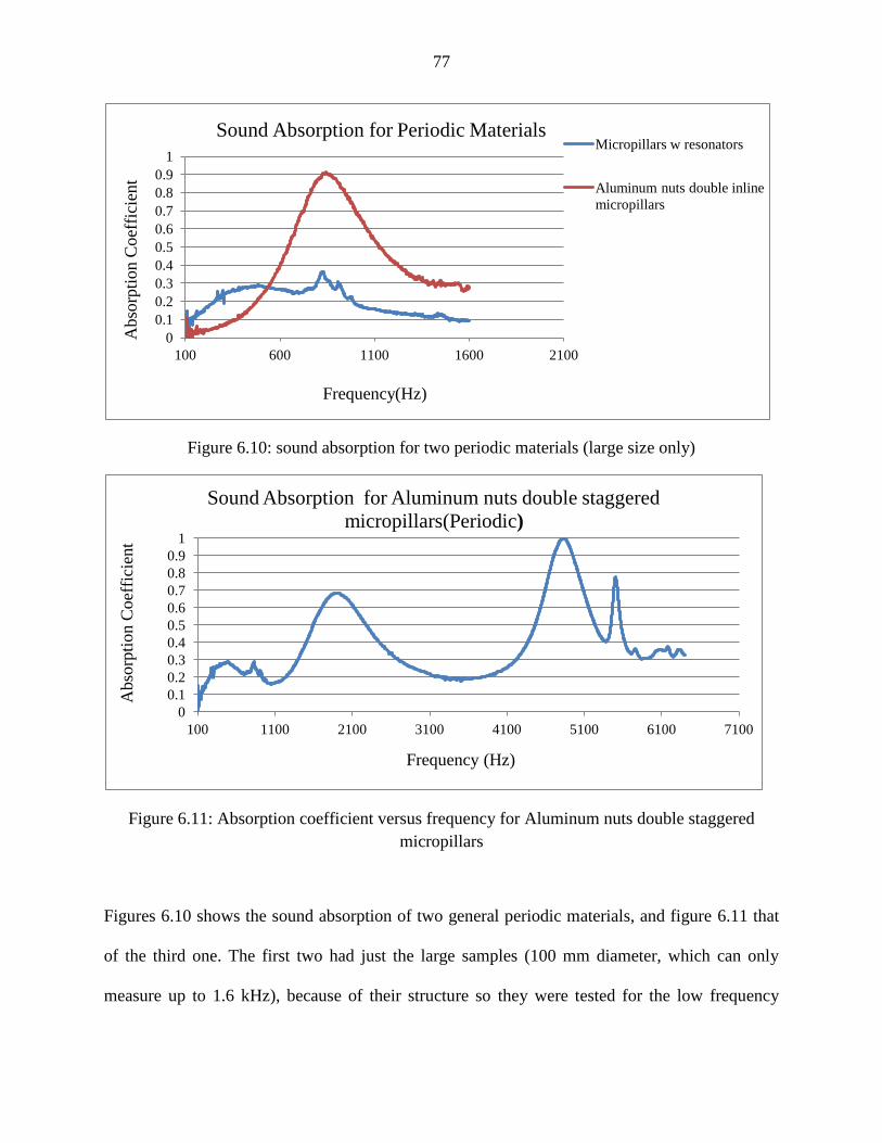
77
Figure 6.10: sound absorption for two periodic materials (large size only)
Figure 6.11: Absorption coefficient versus frequency for Aluminum nuts double staggered
micropillars
Figures 6.10 shows the sound absorption of two general periodic materials, and figure 6.11 that
of the third one. The first two had just the large samples (100 mm diameter, which can only
measure up to 1.6 kHz), because of their structure so they were tested for the low frequency
0
0.1
0.2
0.3
0.4
0.5
0.6
0.7
0.8
0.9
1
100 600 1100 1600 2100
Micropillars w resonators
Aluminum nuts double inline
micropillars
Sound Absorption for Periodic Materials A
bso
rpti
on C
oef
fici
ent
Frequency(Hz)
0
0.1
0.2
0.3
0.4
0.5
0.6
0.7
0.8
0.9
1
100 1100 2100 3100 4100 5100 6100 7100
Sound Absorption for Aluminum nuts double staggered
micropillars(Periodic)
Frequency (Hz)
Abso
rpti
on C
oef
fici
ent
78
range, the absorption for the double in-line micropillars is strongly resonant. Its absorption
exceeds 0.5 only between 600 and 1200 Hz, in the low-to-medium frequency range. The double
staggered micropillars also manifests resonance behavior and shows absorption above 0.5 for the
frequency ranges 1600-2500 Hz and 4500-5200Hz. It seems clear that specific design of the
component parts in terms of mass and stiffness distributions may be used to tailor the frequency
ranges where high absorptions may be attained. The structure with internal resonators does not
show good absorption anywhere in the 0-1600 Hz range and its use will probably be in
connection with vibration rather than acoustics. The presence of many local component systems
in the last two structures leads to many internal resonances and absorption peaks.
The micropillar constructions show very high absorptions ant frequency bands where their
particular constructions allow them to resonate with relatively large amplitudes, but as non-
absorbers ,they have weak absorption at other frequencies
6.3 VIBRATION RESULTS
On account of the modal effect of distributed mass structures, even a simple, isotropic panel will
have an infinite number of vibration modes. In addition, when internal components exist which
may also vibrate locally, the responses become even more. This effect is seen in all the vibration
results.
In these results we will show only one complete set of results for one sample in each group
due to the large amount of results. However the complete results for the remaining samples will
be shown in tables. On the other hand one more complete set of results for another sample from
each group will be shown in appendix D at the end of this dissertation, a comparison between

79
results for the whole set of each group will be shown after the results of the selected material of
each group has finished.
The results will be in the following sequence:
1. Stability diagram which shows the exact natural frequencies for the structure using
PULSE Reflex.
2. FRF, Phase and Coherence.
3. FRF from RADIOSS for samples computed.
4. Finite element results from Abaqus including the 1st three mode shapes
5. Matlab results for samples computed
6. Diagrams for the following
6.1 Maximum deflections for the 1st three modes
6.2 Damping ratios for the 1st three modes
6.3 Compatibility between results (experimental and numerical)
6.4 Comparisons between the results for the whole set of samples for each group
7. Tables to show the results for the whole group
6.3.1 HONEYCOMB MATERIALS
The honeycomb materials were tested for vibration behavior using PULSE 16.1. To verify the
experimental results, finite element simulation was used to get the natural frequencies, and mode
shapes for each of the samples. The analysis of the vibration and acoustics of honeycomb
materials involves at least four key stiffness and strength properties in each direction-
longitudinal and transverse. These properties are Young’s modulus, shear modulus tensile
strength, and compressive strength. The failure modes of the honeycomb are usually local
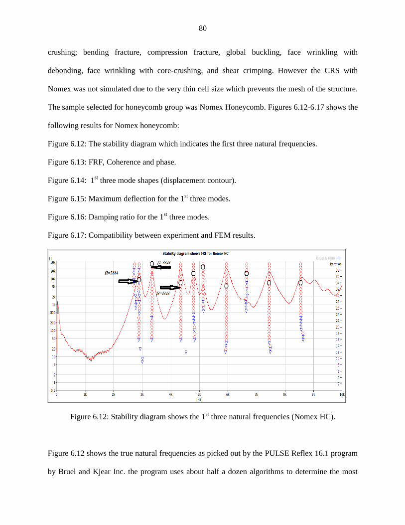
80
crushing; bending fracture, compression fracture, global buckling, face wrinkling with
debonding, face wrinkling with core-crushing, and shear crimping. However the CRS with
Nomex was not simulated due to the very thin cell size which prevents the mesh of the structure.
The sample selected for honeycomb group was Nomex Honeycomb. Figures 6.12-6.17 shows the
following results for Nomex honeycomb:
Figure 6.12: The stability diagram which indicates the first three natural frequencies.
Figure 6.13: FRF, Coherence and phase.
Figure 6.14: 1st three mode shapes (displacement contour).
Figure 6.15: Maximum deflection for the 1st three modes.
Figure 6.16: Damping ratio for the 1st three modes.
Figure 6.17: Compatibility between experiment and FEM results.
Figure 6.12: Stability diagram shows the 1st three natural frequencies (Nomex HC).
Figure 6.12 shows the true natural frequencies as picked out by the PULSE Reflex 16.1 program
by Bruel and Kjear Inc. the program uses about half a dozen algorithms to determine the most

81
accurate locations of the resonance frequencies, taking a host of parameters into account. Thus,
even if some of the peaks indicated don’t appear to be obvious yet they would still be the best
ones from these detailed computations. However in this figure the peaks are all clear. The FRF is
multi-peaked because of multiple resonances of the vibration of these complex structures.
Figure 6.13: FRF, Coherence and phase (Nomex HC)
The coherence values are virtually at the maximum level (unity value) throughout the frequency
range, thus indicating the accuracy of the results.
(Displacement contour) Mode1 Mode 2 Mode3
Figure 6.14: 1st three mode shapes (displacement contour, Nomex HC)
The first three mode shapes as can be seen in figure 6.14 conform to the pattern observed for a
circular plate in bending vibration, showing the two diametral nodes for the first mode, one
circular node for the second mode and three diametral nodes for the third mode. The contour
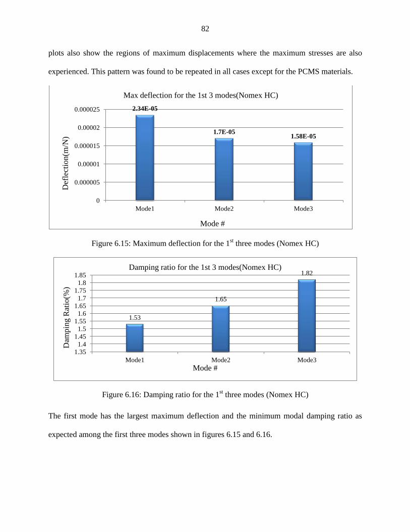
82
plots also show the regions of maximum displacements where the maximum stresses are also
experienced. This pattern was found to be repeated in all cases except for the PCMS materials.
Figure 6.15: Maximum deflection for the 1st three modes (Nomex HC)
Figure 6.16: Damping ratio for the 1st three modes (Nomex HC)
The first mode has the largest maximum deflection and the minimum modal damping ratio as
expected among the first three modes shown in figures 6.15 and 6.16.
2.34E-05
1.7E-05 1.58E-05
0
0.000005
0.00001
0.000015
0.00002
0.000025
Mode1 Mode2 Mode3
Max deflection for the 1st 3 modes(Nomex HC)
Def
lect
ion(m
/N)
Mode #
1.53
1.65
1.82
1.35
1.4
1.45
1.5
1.55
1.6
1.65
1.7
1.75
1.8
1.85
Mode1 Mode2 Mode3
Damping ratio for the 1st 3 modes(Nomex HC)
Mode #
Dam
pin
g R
atio
(%)

83
Figure 6.17: Compatibility between experiment and FEM results (Nomex HC)
For the first two modes(figure 6.17), the maximum deviation of the computed resonance
frequency from the experimental is less than 4%, and even for the third mode the difference is
less than 11%. These again attests to the accuracy of the experimental work and to the
appropriateness of using the curve fit approach for the few property values that could not
otherwise be obtained.
Table 6.1 compares the number of elements, number of nodes and element type from finite
element simulations for the honeycomb group; on the other hand the number of peaks from
experimental results is shown to indicate modal densities of these samples over a specified
frequency range.
2884
3341
4343
2983
3407
3866
0
500
1000
1500
2000
2500
3000
3500
4000
4500
5000
mode1 mode2 mode3
exp
FEM
Fre
qu
ency
(Hz)
Compatibility between exp and FEM results
Mode #

84
Table 6.1: Comparison between honey comb samples according to number of nodes,
elements and element type, with the modal densities
Material #of
nodes
#of
elements
Element type # of peaks in the frequency
range(0-6.4 kHz)
AL HC 89762 294252 C3D4 3
HC A 98676 199812 S3 5
HC B 77390 249818 C3D4 7
HC C 57862 188487 C3D4 4
HC D 31123 65838 S3 9
Nomex HC 89412 179810 S3 6
CRS
w/Nomex*
4
*: the software was not able to mesh it because the cell thickness was too small
Table 6.2 compares the vibration results for the honeycomb group, and then these results are
shown in a graphical representation in order to give a better understanding about the behavior of
these structures.
Table 6.2: Vibration results for Honeycomb structures
Material Mode# Damping
ratio(η)%
Natural frequency(Hz) Max
deflection(m/N) Experimental Finite
Element
AL HC 1 1.86 3547 3291(7%)* 0.00000541
2 3.39 5570 5262(5.5%) 0.00000176
3 2.14 6209 5908(4.8%) 0.0000027
HC A 1 0.79 4888 5000(2.2%) 0.00000565
2 2.48 6458 6074(6%) 0.000000855
3 1.81 9284 8557(7.8%) 0.00000324
HC B 1 4.5 2154 1863(13%) 0.0000318
2 7.6 2907 3152(8%) 0.0000262
3 4.7 3476 3817(9.8%) 0.0000272
HC C 1 0.96 1871 2022(8%) 0.000113
2 1.46 3288 3468(5%) 0.0000287
3 1.69 4599 4040(12%) 0.0000167
HC D 1 1.15 1875 1856(1%) 0.000113
2 3.63 2061 2265(9.8%) 0.0000177
3 4.56 2356 2359(0.1%) 0.00000572
Nomex Hc 1 1.53 2884 2983(3.4%) 0.0000234
2 1.65 3341 3407(1.9%) 0.000017
3 1.82 4343 3866(10.9%) 0.0000158
CRS
w/Nomex**
1 0.86 878 - 0.000158
2 1.51 1483 - 0.0000849
3 1.9 2892 - 0.0000116
* : (%) Percentage error between experimental and finite element results
**: The material couldn’t be simulated in FEM because of very thin core thickness

85
Figures 6.18-6.22 show the comparisons between the different samples of the honeycomb
materials as follows:
Figure 6.18: Comparison between numbers of elements
Figure 6.19: Comparison between natural frequencies for the 1st three modes
Figure 6.20: Comparison between maximum deflections for the 1st three modes
Figure 6.22: Comparison between damping ratios for the 1st three modes
Figure 6.23: Comparison between modal densities
Figure 6.18: Comparison between numbers of elements (Honeycomb group)
Figure 6.18 shows the various numbers of elements that were used to simulate the different
samples on account of the relative complexities of their structures, and the available computing
resources. These numbers vary between almost 66,000 to almost 300,000, showing that these
structures are quite complex to model if reasonable results are desired.
65838
179810 188487 199812
249818
294252
0
50000
100000
150000
200000
250000
300000
350000
HC D Nomex HC HC C HC A HC B AL HC
Number of elements (Honeycomb group)
Num
ber
of
Ele
men
ts
Material

86
Figure 6.19: Comparison between 1st three natural frequencies (Honeycomb group)
The natural frequency is an approximate expression of the stiffness distribution relative to
mass distribution in the structure. The comparison of this parameter for the honeycomb
structures is shown in figure 6.19, here a monotonic arrangement for mode 1 (the fundamental,
and usually most important for vibration consideration) is constructed. All other things being
equal, this ratio is often loosely correlated with stiffness. Thus, the CRS/Nomex honeycomb is
the “softest” structure in the group, while the honeycomb A (glass-epoxy skins and aluminum
honeycomb core) is the “stiffest”. The differences in construction give us possible design latitude
in tailoring our desired natural frequencies. It must also be remembered that the skins are
normally bonded to honeycomb cores with adhesives. The strength of such adhesives and the
quality of bonding both affect the relative softness or stiffness
Mode1
Mode2
Mode3 0
2000
4000
6000
8000
10000
CR
S
w/N
om
ex
HC
C
HC
D
HC
B
No
mex
HC
AL
HC
HC
A
Mode1
Mode2
Mode3
Fre
qu
ency
(Hz)
Comparison between natural frequencies(Honeycomb group)
Material

87
Figure 6.20: Comparison between maximum deflections for the 1st three modes(Honeycomb
group)
As it can seen from figure 6.20, mode one for all the samples is the dominant mode where the
maximum deflection is largest. Since stress is proportional to deflection at a point, this also
indicates that the maximum stresses are experienced in the mode 1 of vibration resonance. Hence
if steps are taken to ameliorate mode 1 effects, then it would not be necessary to worry about the
immediate higher modes, from the point of view of damage.
Figure 6.21: Comparison between damping ratios for the 1st three modes(Honeycomb group)
mode1
mode2
mode3 0
0.00005
0.0001
0.00015
0.0002
AL
HC
HC
A
No
mex
HC
HC
B
HC
D
HC
C
CR
S
w/N
om
ex
mode1
mode2
mode3
Def
lect
ion(m
/N)
Comparison between maximum deflection(Honeycomb group)
Material
mode1
mode3
0
2
4
6
8
HC A CRS
w/Nomex
HC C HC D Nomex
HC
AL HC HC B
mode1
mode2
mode3
Comparison between damping ratios(Honeycomb group)
Dam
pin
g ra
tio(%
)
Material

88
The modal damping ratio (figure 6.21) is least for mode 1 for all the honeycomb materials. The
modal damping effectively contributes to the restraint of motion. For each material the results for
maximum deflection and damping ratio are consistent in the sense that relatively high deflections
are generally associated with relatively low damping ratios.
Figure 6.22: Comparison between modal densities (Honeycomb group)
Figure 6.22 shows the modal density, which is a measure of the complexity of the structure, it is
effectively indicated here by the number of resonant peaks in a given frequency band. Arranged
monotonically, it is seen that the aluminum honeycomb seems to be the least complex while
honeycomb D (polyester skins and aramid core), appears to be the most complex. Complexity is
a cost in terms of material, labor and delay time charges, and this would normally go into
decision making before particular structures are deployed.
3
4 4
5
6
7
9
0
1
2
3
4
5
6
7
8
9
10
AL HC HC C CRS
w/Nomex*
HC A Nomex HC HC B HC D
Modal density
# o
f P
eak
s
Materails

89
6.3.2 MONOLITHIC AND SANDWICH MATERIALS
The monolithic and sandwich materials were tested for vibration behavior using PULSE 16.1. To
verify the experimental results, finite element simulation was used to get the natural frequencies,
and mode shapes, for each of the samples. The sample selected for monolithic group was single
layer Lexan with large holes while USIL light was selected as a sandwich sample. Figures 6.23
to 6.29 show the following results for single layer Lexan with large holes:
Figure 6.23: The stability diagram which indicates the first three natural frequencies
Figure 6.24: FRF, Coherence and phase
Figure 6.25: FRF results from RADIOSS
Figure 6.26: 1st three mode shapes (displacement contour)
Figure 6.27: Maximum deflection for the 1st three modes
Figure 6.28: Damping ratio for the 1st three modes
Figure 6.29: Compatibility between experiment and FEM results
Figure 6.23: The stability diagram shows the first three natural frequencies (1 Layer Lexan with
large holes)

90
The peaks in the stability diagram as shown in figure 6.23 are distinct and more than in the
comparable solid sample (3 peaks) as can seen in appendix D, the amplitudes at the peaks for this
sample are higher than for the solid one. This is as expected because this sample has been
rendered more flexible and softer by the punching of holes in it.
Figure 6.24: FRF, Coherence and phase (1 Layer Lexan w/large holes).
Figure 6.24 shows a good coherence values (unity) over the frequency band, in addition to this,
the phase tends to be around 900 at resonance frequencies which is again an indication of the
accuracy of the experimental work. The top diagram of figure 6.24, which is the FRF is only a
more diffuse image of the stability diagram of figure 6.23, which has been discussed.

91
Figure 6.25: FRF results from RADIOSS (1 Layer Lexan w/large holes).
The finite element results (Radioss and Abaqus) agree very well with the experimental
results(less than 5% for the first mode) as it can be seen from figures 6.24 and 6.25, this signifies
that the experiments were carried out in sufficient accuracy.
(Displacement Contour) Mode1 Mode2 Mode3
Figure 6.26: 1st three mode shapes (displacement contour, 1 Layer Lexan w/large holes).
The first three mode shapes (figure 6.26) conform to the pattern observed for a circular plate in
bending vibration, showing the two diametral nodes for the first mode, one circular node for the
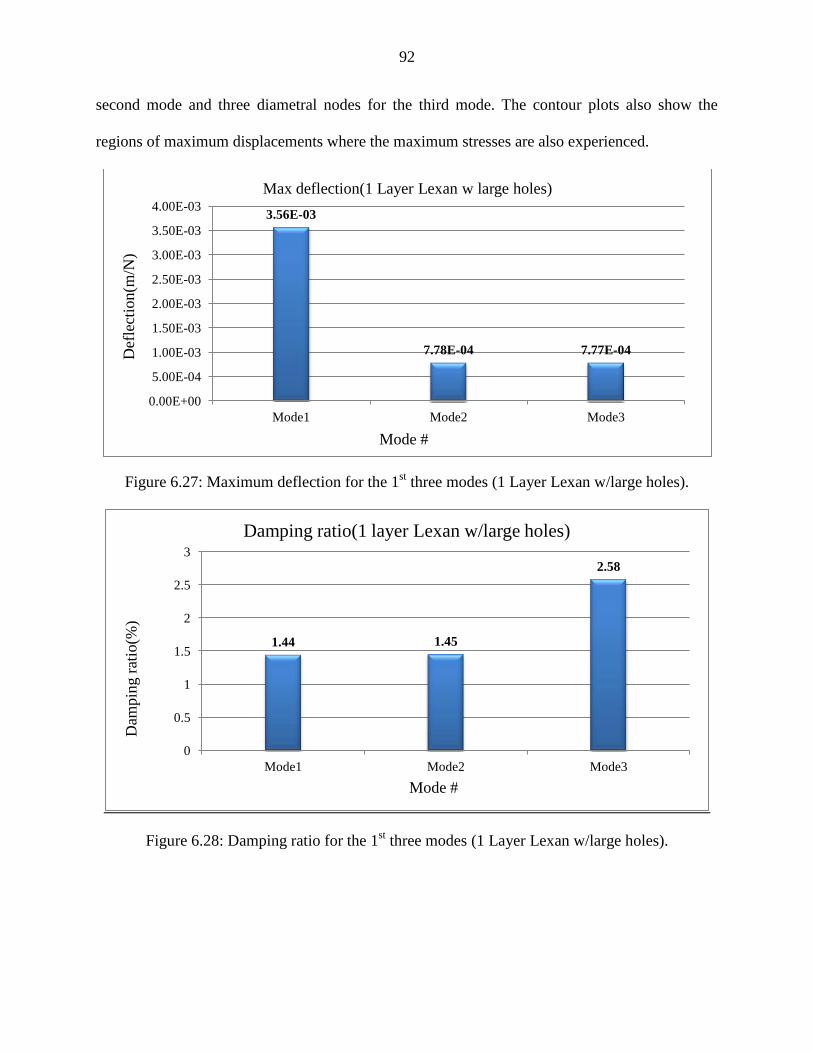
92
second mode and three diametral nodes for the third mode. The contour plots also show the
regions of maximum displacements where the maximum stresses are also experienced.
Figure 6.27: Maximum deflection for the 1st three modes (1 Layer Lexan w/large holes).
Figure 6.28: Damping ratio for the 1st three modes (1 Layer Lexan w/large holes).
3.56E-03
7.78E-04 7.77E-04
0.00E+00
5.00E-04
1.00E-03
1.50E-03
2.00E-03
2.50E-03
3.00E-03
3.50E-03
4.00E-03
Mode1 Mode2 Mode3
Max deflection(1 Layer Lexan w large holes)
Def
lect
ion
(m/N
)
Mode #
1.44 1.45
2.58
0
0.5
1
1.5
2
2.5
3
Mode1 Mode2 Mode3
Damping ratio(1 layer Lexan w/large holes)
Dam
pin
g r
atio
(%)
Mode #

93
The maximum deflections and the modal damping ratios as it can be seen from figures 6.27 and
6.28 are consistent for each mode in that high values of deflections correspond to low values of
modal damping. Mode one manifests the largest maximum deflection as expected.
Figure 6.29: Compatibility between experiment and FEM results (1 Layer Lexan w/large holes).
Figure 6.29 shows the very good agreement between experimental and finite element results for
each of the first three modes that were considered. This suggests that the experiments were
carefully and accurately carried out.
As mentioned before USIL Light was selected to represent the sandwich structures, figures 6.30
to 6.37 shows the following results for USIL Light:
Figure 6.30: The stability diagram which indicates the first three natural frequencies
Figure 6.31: FRF, Coherence and phase
Figure 6.32: FRF results from RADIOSS
Figure 6.33: 1st three mode shapes (displacement contour)
Figure 6.34: 1st three mode shapes using Matlab
256
409
599
269
411
624
0
100
200
300
400
500
600
700
Mode1 Mode2 Mode3
Exp
FEM
Fre
quen
cy(H
z)
Compatibilty between FEM and exp(1 layer Lexan w large holes)
Mode #

94
Figure 6.35: Maximum deflection for the 1st three modes
Figure 6.36: Damping ratio for the 1st three modes
Figure 6.37: Compatibility between experiment and FEM results
Figure 6.30: The stability diagram which indicates the first three natural frequencies
Figure 6.31: FRF, Coherence and phase

95
Figure 6.32: FRF results from RADIOSS
The FRF diagram shown in figure 6.30 obtained from PULSE Reflex shows very crisp peaks and
well-spaced out resonances suggesting that the material was manufactured with precision. The
coherence values (figure 6.31), are virtually at the maximum level and the phase at resonance
(about 900), the FRF from RADIOSS program (Altair Inc.), which is clear in figure 6.32, shows
a very good match with the experiment. It should be noted that the material was treated as a
composite within the RADIOSS program, putting in the appropriate set of material properties for
the skin and the core separately.
(Displacement Contour) Mode1 Mode2 Mode3
Figure 6.33: 1st three mode shapes (displacement contour)

96
Figure 6.34: 1st three mode shapes using Matlab
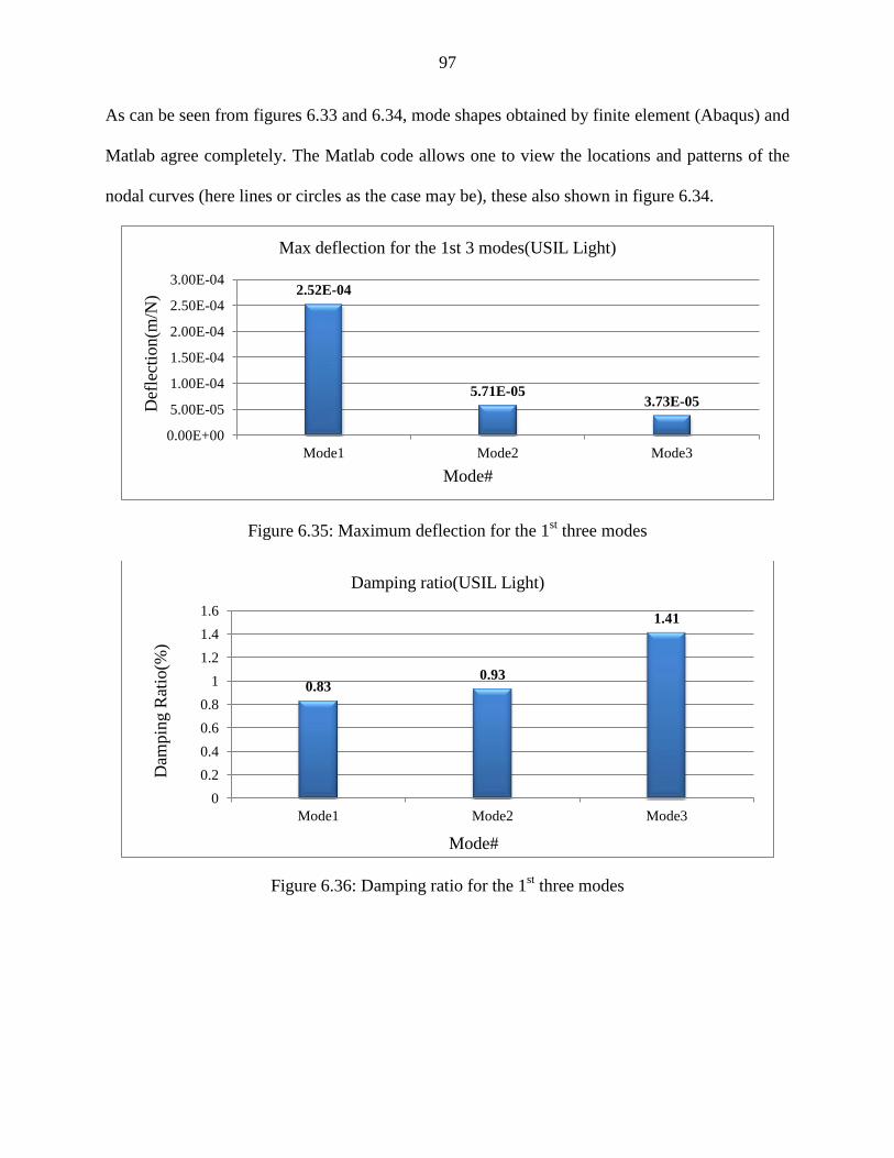
97
As can be seen from figures 6.33 and 6.34, mode shapes obtained by finite element (Abaqus) and
Matlab agree completely. The Matlab code allows one to view the locations and patterns of the
nodal curves (here lines or circles as the case may be), these also shown in figure 6.34.
Figure 6.35: Maximum deflection for the 1st three modes
Figure 6.36: Damping ratio for the 1st three modes
2.52E-04
5.71E-05 3.73E-05
0.00E+00
5.00E-05
1.00E-04
1.50E-04
2.00E-04
2.50E-04
3.00E-04
Mode1 Mode2 Mode3
Max deflection for the 1st 3 modes(USIL Light)
Def
lect
ion(m
/N)
Mode#
0.83 0.93
1.41
0
0.2
0.4
0.6
0.8
1
1.2
1.4
1.6
Mode1 Mode2 Mode3
Damping ratio(USIL Light)
Dam
pin
g R
atio
(%)
Mode#

98
Once more it can be seen (figures 6.35, 6.36) that mode1 is dominant with the largest value of
maximum displacement among the first three modes. Its modal damping ratio is also the least in
this frequency range.
Figure 6.37: Compatibility between experiment and numerical methods results
Figure 6.37 shows very good agreement between experimental and four numerical methods.
Excluding the calculation, the maximum deviations of the numerical methods from experimental
are 4.6%, 8.7%, 0.2% for modes1to 3 respectively. For the calculations and Matlab method,
effective values of Young’s modulus E, Poisson’s ration ν, and density ρ were utilized. The
effective values were based upon the relative thicknesses. Also, the calculation approach
employed the Rayleigh energy method to obtain resonance frequencies, while the Matlab
solution utilized Bessel functions, which generally give more accurate solutions. Accordingly,
the calculation results deviated a little further than the other numerical results. Thus, taking the
calculation method into account, the maximum deviations of the numerical methods from
experimental are 10%, 9.5%, 4.7% for modes1to 3 respectively.
975
1709
2134
931
1555
2136
877
1515
2042
963
1500
2198
930
1560
2140
0
500
1000
1500
2000
2500
Mode 1 Mode 2 Mode 3
exp
FEM
Calculation
Matlab
RADIOSS

99
Table 6.3 below compares the number of elements, number of nodes and element type from
finite element simulations for the sandwich and monolithic group; on the other hand the number
of peaks from experimental results is shown to indicate modal densities of these samples over a
specified frequency range(0-1.6kHz for monolithic and 0-6.4kHz for sandwich).
Table 6.3: Comparison between sandwich and monolithic samples according to number of nodes,
elements and element type, with the modal densities
Material # of nodes #of elements Element type #of peaks(0-
1.6kHz
monolithic,0-
6.4kHz
Sandwich)
Sandwich
Materials
CRS w/LE
5208
91697 20480 C3D20 4
USIL Light 70733 15360 C3D20 6
3Layer
Lexan1
49098 81876 C3D6 12
5Layer
Lexan3
48384 78852 C3D6 14
Monolithic
Materials
Single Layer
Solid Lexan
7154 3536 C3D20 5
1 Layer Lexan
w/small holes
80156 113784 C3D6 6
1 Layer Lexan
w/membrane
30977 908(membrane)
44232(Lexan)
S3(membrane)
C3D6(Lexan)
5
1 Layer Lexan
w/large holes
80156 113784 C3D6 5
CRS Alone 5931 3848 C3D8I 5
Table 6.4 compares the vibration results for the sandwich and monolithic group, and then these
results are shown in a graphical representation in order to give a better understanding about the
behavior of these structures.

100
Table 6.4: Vibration results for Sandwich and Monolithic structures
Material Mode# Damping
Ratio (%)
Natural Frequency(Hz) Max
deflection(m/N) Experiment Finite
Element
San
dw
ich
Mat
eria
ls
Cold Rolled
Steel
w/LE5208
1 1.19 3223 3139(2.6%) 0.0000058
2 1.65 4726 4617(2.3%) 0.00000154
3 1.95 5289 5354(1.2%) 0.00000161
USIL Light 1 0.83 970 931(4%) 0.000252
2 0.93 1706 1555(8.8%) 0.0000571
3 1.41 2115 2136(0.1%) 0.0000373
2 layer solid
Lexan
1 2.67 598 621(3.8%) 0.00065785
2 3.51 732 1115(34%) 8.86696E-05
3 3.38 1042 1432(27%) 0.00012856
3Layer
Lexan1
1 1.57 768 838(9%) 0.000162
2 1.73 1153 1508(23%) 2.92E-05
3 1.64 1514 1914(21%) 4.47E-05
5Layer
Lexan2
1 0.46 1271 1358(6.8%) 7.79E-05
2 1.54 1955 2420(19%) 2.12E-05
3 2.41 2784 3004(7.3%) 1.72E-05
Mo
no
lith
ic M
ater
ials
1 layer solid
Lexan
1 1.32E+00 310 313(0.9%) 1.67E-03
2 2.70E+00 581 563(3%) 3.87E-04
3 1.41E+00 715 728(1.8%) 6.19E-04
1 Layer
Lexan
w/small holes
1 1.50E+00 303 318(5%) 2.20E-03
2 3.58E+00 556 559(0.5%) 0.000447
3 1.65E+00 704 736(4.5%) 0.000538
1 Layer
Lexan
w/membrane
1 1.47E+00 290 322(11%) 2.32E-03
2 2.24E+00 526 574(9%) 2.96E-04
3 2.05E+00 681 746(9.5%) 5.46E-04
1 Layer
Lexan
w/large holes
1 2.58E+00 256 269(5%) 3.56E-03
2 1.45E+00 409 411(0.5%) 7.78E-04
3 1.44E+00 599 624(4%) 7.77E-04
CRS Alone 1 0.76 355 333(6%) 0.00249
2 0.46 411 553(25%) 0.00184
3 0.24 863 772(10%) 0.00178
1: Solid-Membrane-Solid 2: Solid-3 Layers w/Small Holes-Solid
It should be mentioned here that, as shown in table 6.4, the percentage error in multi layer Lexan
samples was high and this is due to a number of reasons. The gluw (“Supergluw”) between the
layers did not cure strongly enough, and we had to assemble and disassemble the unit many
times to do the experiments of different configurations, hence, air pockets and delaminations
could not be ruled out for our Lexan structures.

101
Figures 6.38 to 6.42show the comparisons between the different samples of the monolithic
materials as follows:
Figure 6.38: Comparison between numbers of elements
Figure 6.39: Comparison between natural frequencies for the 1st three modes
Figure 6.40: Comparison between maximum deflections for the 1st three modes
Figure 6.41: Comparison between damping ratios for the 1st three modes
Figure 6.42: Comparison between modal densities
Figure 6.38: number of elements for monolithic materials
The number of elements for monolithic materials(figure 6.38) depend upon the architecture, as
can be seen from figure 6.38 the Lexan with holes have more elements than solid Lexan and this
is due to the fact that the holes make the structure more complex and therefore it needs more
elements to mesh it.
3536
113784
44232
113784
3848
0
20000
40000
60000
80000
100000
120000
Single Layer Solid
Lexan
1 Layer Lexan
w/small holes
1 layer lexan
w/membranne
1 Layer Lexan
w/large holes
CRS Alone
Number of elements( Monlothic materials)
# o
f el
emen
ts
Material

102
Figure 6.39: Comparison between natural frequencies for the 1st three modes
The modal resonance frequencies experienced in each mode of the Lexan samples as can be seen
in figure 6.39 seem to follow the order of the values of overall flexibility as would be expected.
The more material is removed from the solid Lexan, the more flexible the sample becomes, and
the less the resonance frequencies. No direct comparisons could be drawn between the Lexan
and the CRS because of material and thickness differences. It follows that material addition,
deletion, or substitution within the sample could be utilized to alter resonance frequencies and
deflections.
mode1
mode2
mode3
0
200
400
600
800
1000
1 Layer
Lexan
w/large holes
1 Layer
Lexan
w/membrane
1 Layer
Lexan
w/small holes
1 layer solid
Lexan CRS Alone
mode1
mode2
mode3
Comparison between natural frequencies(Monolothic Materials) F
requen
cy(H
Material
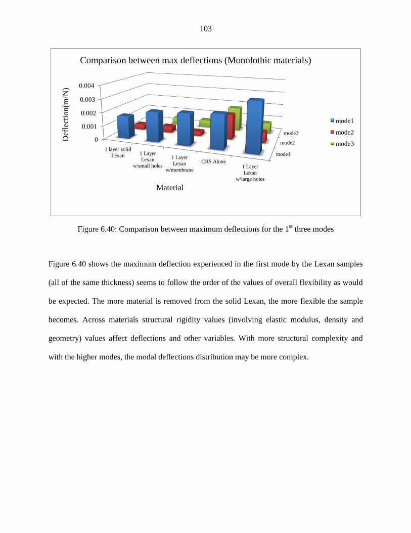
103
Figure 6.40: Comparison between maximum deflections for the 1st three modes
Figure 6.40 shows the maximum deflection experienced in the first mode by the Lexan samples
(all of the same thickness) seems to follow the order of the values of overall flexibility as would
be expected. The more material is removed from the solid Lexan, the more flexible the sample
becomes. Across materials structural rigidity values (involving elastic modulus, density and
geometry) values affect deflections and other variables. With more structural complexity and
with the higher modes, the modal deflections distribution may be more complex.
mode1
mode2
mode3
0
0.001
0.002
0.003
0.004
1 layer solid
Lexan 1 Layer
Lexan
w/small holes
1 Layer
Lexan
w/membrane
CRS Alone 1 Layer
Lexan
w/large holes
mode1
mode2
mode3
Comparison between max deflections (Monolothic materials) D
efle
ctio
n(m
/N)
Material

104
Figure 6.41: Comparison between damping ratios for the 1st three modes
The damping ratio of the metallic CRS is very small as expected of this class of materials. The
modal damping ratios (figure6.41) are much higher for the plastic polycarbonate Lexan material
than for the CRS. The more solid the material is, it appears that the less the mode-1 damping.
For higher modes this may not be guaranteed as the mode shapes vary widely across the modes.
Some modes involve predominantly shearing motion and some bending motion.
mode1
mode2
mode3
0
1
2
3
4
CRS Alone 1 layer solid
Lexan 1 Layer
Lexan
w/membrane
1 Layer
Lexan
w/small holes
1 Layer
Lexan
w/large holes
mode1
mode2
mode3
Comparison between damping ratios(Monolothic materials) D
ampin
g r
atio
(%)
Material

105
Figure 6.42: Comparison between modal densities
The number of peaks in the (0-1.6 kHz) is practically the same for all the samples. This is
believed to be due to the fact that structures are simple disk in each case. Complexity is
introduced by the holes drilled into the sample but apparently this does not begin to be
significant until the case of Lexan with small holes. In that case we have the largest number of
holes (21). This means that from the point of view of manufacturing costs any of these structures
could be utilized based on other factors. Figure 6.42shows these facts.
Figures 6.43 to 6.47shows the comparisons between the different samples of the sandwich
materials as follows:
Figure 6.43: Comparison between numbers of elements
Figure 6.44: Comparison between natural frequencies for the 1st three modes
Figure 6.45: Comparison between maximum deflections for the 1st three modes
Figure 6.46: Comparison between damping ratios for the 1st three modes
Figure 6.47: Comparison between modal densities
5
6
5 5 5
0
1
2
3
4
5
6
7
Single Layer Solid
Lexan
1 Layer Lexan
w/small holes
1 layer lexan
w/membranne
1 Layer Lexan
w/large holes
CRS Alone
Modal density( Monolthic materials,0-1.6kHz) # o
f pea
ks
Material

106
Figure 6.43: Comparison between numbers of elements
From figure 6.43 it may be observed that the Lexan samples shown required a lot more nodes to
mesh them than the CRS and USIL light samples. The first reason for these is that the Lexan
samples are layered structures. Secondly it is also seen that more nodes were required to mesh
the three layer Lexan than the five layer Lexan. This was so because the three layer Lexan had
holes and the membrane film which both took more nodes to numerically define them.
20480 15360
81876 78852
0
10000
20000
30000
40000
50000
60000
70000
80000
90000
CRS w/LE
5208
USIL Light 3Layer Lexan 5Layer Lexan
# o
f el
emen
ts
Number of elements from FEM(Sandwich materilas)
Material

107
Figure 6.44: Comparison between natural frequencies for the 1st three modes
The distribution of the natural frequencies on as shown in figure 6.44 is very regularly
distributed over the first three modes shown, essentially on the basis of stiffness. Thus, since
each Lexan layer is of the same 2mm thickness, the natural frequency of the 3 layer structure is
higher than that of the 2 layers, etc. It may be recalled that theoretically, the square of natural
frequency is proportional to the ratio of the distribution of stiffness to that of mass in the
structure.
mode1
mode2
mode3
0
1000
2000
3000
4000
5000
6000
2 layer solid
Lexan 3Layer Lexan USIL Light
5Layer Lexan Cold Rolled
Steel w/LE5208
mode1
mode2
mode3
Comparison between natural frequencies(Sandwich structures) F
requen
cy(H
z)
Material

108
Figure 6.45: Comparison between maximum deflections for the 1st three modes
The maximum deflection values (figure 6.45) seem to show inverse relationship to the rigidity of
the specimens, as would be expected from fundamental consideration of vibration principles. The
maximum deflection of the CRS is much less than that of any of the Lexan structures because of
the significant difference between their elastic moduli.
mode1
mode2
mode3
0
0.0001
0.0002
0.0003
0.0004
0.0005
0.0006
0.0007
Cold Rolled
Steel
w/LE5208
5Layer Lexan2 3Layer Lexan1
USIL Light 2 layer solid
Lexan
mode1
mode2
mode3
Comparison between max deflection(Sandwich structures) D
efle
ctio
n(m
/N)
Material

109
Figure 6.46: Comparison between damping ratios for the 1st three modes
The modal damping ratio values shown in Figure 6.46 indicate for the Lexan, more thickness
seems to degrade the damping of the structure. The USIL light and CRS/LE 5208 sandwiches
take positions in this arrangement based on their rigidities and the material damping in their
make-up
mode1
mode2
mode3
0
1
2
3
4
5Layer Lexan USIL Light
Cold Rolled
Steel w/LE5208 3Layer Lexan 2 layer solid
Lexan
mode1
mode2
mode3
Comparison between damping ratios(Sandwich structures) D
ampin
g R
atio
(%)

110
Figure 6.47: Comparison between modal densities
The modal density which is shown in figure 6.47 (0-6.4 kHz) for sandwich structures shows up
as four and sex respectively for the CRS and USIL Light structures. This is sparse, showing that
the structures are simple and behaved like well-bonded compact disks. On the other hand the
multi-layer Lexan samples manifested many more resonances in the same frequency interval.
This is due to the presence of several layers and less than perfect adhesive bonding, the presence
of holes and membranes as the case may be. Such additional factors usually add more resonance
peaks to the vibration response of the structure.
6.3.3 PERIODIC CELLULAR MATERIAL STRUCTURES (PCMS) MATERIALS
The PCMS materials were tested for vibration behavior using PULSE 16.1. To verify the
experimental results, finite element simulation was used to get the natural frequencies, and mode
4
6
12
14
0
2
4
6
8
10
12
14
16
CRS w/LE 5208 USIL Light 3Layer Lexan 5Layer Lexan
Modal density (Sandwich material, 0-6.4kHz)
# o
f p
eaks
Material

111
shapes, for each of the samples. The sample selected for PCMS group was Aluminum prismatic
Microtruss (circular sample). It should be mentioned here that this sample has been cut from a
rectangular sample which we got from the Cellular material Inc (CMI), to fit inside the
impedance tube, we noticed that it was very critical to select the coordinates of the cut as it
affects the vibration behavior of the material as we will see in the parametric study section later.
Figures 6.48 through 6.54 shows the results for this sample as follows:
Figure 6.48: The stability diagram which indicates the first three natural frequencies
Figure 6.49: FRF, Coherence and phase
Figure 6.50: FRF results from RADIOSS
Figure 6.51: 1st three mode shapes (displacement contour)
Figure 6.52: Maximum deflection for the 1st three modes
Figure 6.53: Damping ratio for the 1st three modes
Figure 6.54: Compatibility between experiment and FEM results
Figure 6.48: The stability diagram which indicates the first three natural frequencies

112
Figure 6.49: FRF, Coherence and phase
Figure 6.50: FRF results from RADIOSS

113
Figures 6.48 show the stability diagram, a display of the most accurate rendering of the FRF with
different useful annotations. The fact of the structure’s complexity is obvious, on account of
having many resonances. The resonances are well spaced out and distinct, suggesting that the
bending vibration modes are clear and practically free of mixed modes and distortions. From
figure 6.49 we observe that the virtually universal unity value of the coherence suggests
excellent experimentation, and the phase record is unequivocal in showing the true peaks. Figure
6.50 which was obtained from the RADIOS program of Altair Inc. corroborates the experimental
PULSE Bruel & Kjaer experimental results.
(Displacement contour) Mode1 Mode2 Mode3
Figure 6.51: 1st three mode shapes (displacement contour)
It is obvious from the mode shapes shown in figure 6.51 that the deflections experienced by the
upper and lower skins of the structure tend to be quite different. This is due to the disconnection
in the core structure joining the skins together. This hanging lip is quite visible in each of the
modes. This translates to freedom of motion for the unconnected edge which therefore
experiences the maximum displacement, as also shown by the bright colors in the displacement
contour legend. It is therefore not surprising that the mode shapes of this structure with a cut are
not identical to those of a completely connected structure such as the rectangular sample which
shall be mentioned in the section on parametric studies.

114
This behavior constitutes a very important point with respect to the extraction of parts of
different shapes from a block of material that may be available in the engineering store.
Figure 6.52: Maximum deflection for the 1st three modes
Figure 6.53: Damping ratio for the 1st three modes
Figures 6.52 and 6.53 show that the maximum deflection decrease progressively from mode one
to mode three, whereas the modal damping ratio behaves on the opposite way. The damping ratio
1.28E-05
8.72E-06
1.55E-06
0
0.000002
0.000004
0.000006
0.000008
0.00001
0.000012
0.000014
Mode1 Mode2 Mode3
Max deflection(Al prismatic circular microtruss)
Def
lect
ion
(m/N
)
Mode #
0.1
0.15
0.39
0
0.05
0.1
0.15
0.2
0.25
0.3
0.35
0.4
0.45
Mode1 Mode2 Mode3
Damping ratio(Al prismatic circular microtruss)
Dam
pin
g R
atio
(%)
Mode #

115
values are very reasonable for an aluminum structure, and their sequence shows that the
fundamental mode appears to be the most important for the deformation history of this structure.
It may be recalled that stress is generally proportional to deflection.
Figure 6.54: Compatibility between experiment and FEM results
Figure 6.54 clearly shows the good agreement between experimental and FEM Abaqus results
for natural frequencies. This agreement is considered quit good in light of the fact that it proved
impossible to obtain a numerical cut to coincide exactly with the experimental specimen. The
percentage deviation from experimental values varied from 5.3% for mode one through 8.6% for
mode two to 12% for mode three. The RADIOSS results were not included in this figure because
of the limitation on our computing resources restricted us to the use of only one node for the
RADIOSS computations.
Table 6.5 compares the number of elements, number of nodes and element type from finite
element simulations for the PCMS group; on the other hand the number of peaks from
experimental results is shown to indicate modal densities of these samples over a specified
frequency range.
9507 10411
11005
8997
11314 12364
0
2000
4000
6000
8000
10000
12000
14000
Mode1 Mode2 Mode3
Exp
FEM
Fre
quem
cy(H
z)
Compatibilty between exp and FEM(Al prismatic circular microtruss)
Mode #

116
Table 6.5: Comparison between PCMS samples according to number of nodes, elements and
element type, with the modal densities
Material # of nodes #of elements Element type #of
peaks(0-
10kHz)
Aluminum prismatic
Microtruss
90015 403255 C3D4 14
Stainless steel triangular
honeycomb Microtruss
99938 306280 C3D4 30
Pyramidal aluminum
Microtruss
- - - 26
Table 6.6 compares the vibration results for the PCMS group, and then these results are shown in
a graphical representation in order to give a better understanding about the behavior of these
structures.
Table 6.6: Vibration results for PCMS materials
Material Mode# Damping
ratio(η)%
Natural frequency(Hz) Max
deflection(m/N) Experimental Finite
Element
Alumium
prismatic
microtruss
1 0.1 9507 8997(5.3%) 0.0000128
2 0.39 10411 11314(8.6%) 0.00000872
3 0.15 11005 12364(12%) 0.00000155
Stailess steel
triangular
honeycomb
microtruss
1 0.047 4275 4020(6%) 0.0000125
2 0.15 4521 4172(7.7%) 0.00000214
3 0.083 4769 4327(9%) 0.00000322
Pyramidal*
aluminum
microtruss
1 0.15 2466 - 0.000152
2 0.32 3181 - 0.000046
3 0.38 7143 - 0.00000372
*: the sample was not simulated due to its complexity
Figure 6.55 to 6.59 shows the comparisons between the different samples of the PCMS materials
as follows:
Figure 6.55: Comparison between numbers of elements
Figure 6.56: Comparison between natural frequencies for the 1st three modes
Figure 6.57: Comparison between maximum deflections for the 1st three modes
Figure 6.58: Comparison between damping ratios for the 1st three modes
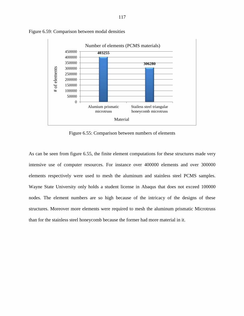
117
Figure 6.59: Comparison between modal densities
Figure 6.55: Comparison between numbers of elements
As can be seen from figure 6.55, the finite element computations for these structures made very
intensive use of computer resources. For instance over 400000 elements and over 300000
elements respectively were used to mesh the aluminum and stainless steel PCMS samples.
Wayne State University only holds a student license in Abaqus that does not exceed 100000
nodes. The element numbers are so high because of the intricacy of the designs of these
structures. Moreover more elements were required to mesh the aluminum prismatic Microtruss
than for the stainless steel honeycomb because the former had more material in it.
403255
306280
0
50000
100000
150000
200000
250000
300000
350000
400000
450000
Alumium prismatic
microtruss
Stailess steel triangular
honeycomb microtruss
Number of elements (PCMS materials)
# o
f el
emen
ts
Material

118
Figure 6.56: Comparison between natural frequencies for the 1st three modes
As can be seen in figure 6.56 for the first two modes the magnitudes of the natural frequency
seems to follow the order of stiffness values. Thus, corresponding frequency values for the
aluminum prismatic structure are higher than those for stainless steel structure, which are in turn
higher than the aluminum pyramidal Microtruss. In the case of mode three it may be recalled that
for higher modes and for more complex structures the frequency distribution may be different.
Mode1
Mode2
Mode3
0
2000
4000
6000
8000
10000
12000
AL Pyramidal
microtruss Stainless steel
Microtruss Aluminum
prismatic
microtruss
Mode1
Mode2
Mode3
Comparison between natural frequencies(PCMS materials)
Fre
quen
cy(H
z)
Material

119
Figure 6.57: Comparison between maximum deflections for the 1st three modes
Figure 6.58: Comparison between damping ratios for the 1st three modes
Figures 6.57 and 6.58 show the maximum deflections and the modal damping values for the first
three modes of vibration. The first figure reveals that the aluminum pyramidal Microtruss
Mode1
Mode2
Mode3
0
0.00005
0.0001
0.00015
0.0002
Stainless steel
Microtruss Aluminum
prismatic
microtruss AL Pyramidal
microtruss
Mode1
Mode2
Mode3
Comparison between max deflection(PCMS materials)
Def
lect
ion
(m/N
)
Material
Mode1
Mode2
Mode3
0.00E+00
5.00E-02
1.00E-01
1.50E-01
2.00E-01
2.50E-01
3.00E-01
3.50E-01
4.00E-01
Stainless steel
Microtruss Aluminum prismatic
microtruss AL Pyramidal
microtruss
Mode1
Mode2
Mode3
Comparison between damping ratios(PCMS materials)
Dam
pin
g R
atio
(%)
Material

120
expediencies significantly more maximum deflection than the other two PCMS materials. This is
understandable because the pyramidal structure consists essentially of two relatively thin skins
connected by a grid of slender metal bars. This construction makes it far more flexible than the
other two. The second figure also shows that the pyramidal Microtruss structure has the highest
modal damping ratio. Although one would have expected the damping to be the minimum, in
fact the numerous bars in the core structure contribute a lot of damping to the movement of the
structure.
Figure 6.59: Comparison between modal densities
Figure 6.59 shows that the entire group of PCMS materials are complex structures manifesting
much higher modal densities than the ones considered earlier. This is a result of their
complicated constructions. As mentioned earlier the cost of high modal density comes in terms
of amplified material, time and labor costs. It can also be seen from the figure that relatively the
construction of the aluminum prismatic Microtruss is about half as complex as the other two.
14
26
30
0
5
10
15
20
25
30
35
Alumium prismatic microtruss Pyramidal aluminum
microtruss
Stailess steel triangular
honeycomb microtruss
Modal density(PCMS materials 0-12.6kHz)
# o
f pea
ks
Material

121
6.3.4 GENERAL PERIODIC MATERIALS
It was not possible to draw these structures using Unigraphics (WSU Student Version) because
of the complexity of these structures; it can be done using other software in the future, so the
results for this group are the experimental results only. The Aluminum nuts double staggered
micropillars is selected as the sample of this group.
Figure 6.60 to 6.64 shows the results for this sample as follows:
Figure 6.60: The stability diagram which indicates the first three natural frequencies.
Figure 6.61: FRF, Coherence and phase.
Figure 6.62: 1st three mode shapes (displacement contour, experimental results).
Figure 6.63: Maximum deflection for the 1st three modes.
Figure 6.64: Damping ratio for the 1st three modes.
Figure 6.60: The stability diagram which indicates the first three natural frequencies

122
Figure 6.61: FRF, Coherence and phase
Figure 6.60 shows the stability, diagram, a display of the most accurate rendering of the FRF
with different useful annotations. The fact of the structure’s complexity is obvious, on account of
having many resonances. The resonances are well spaced out and distinct, suggesting that the
bending vibration modes are clear and practically free of mixed modes and distortions. From
figure 6.61 we observe that the virtually universal unity value of the coherence suggests
excellent experimentation, and the phase record is unequivocal in showing the true peaks.
Figure 6.62: 1st three mode shapes (displacement contour)
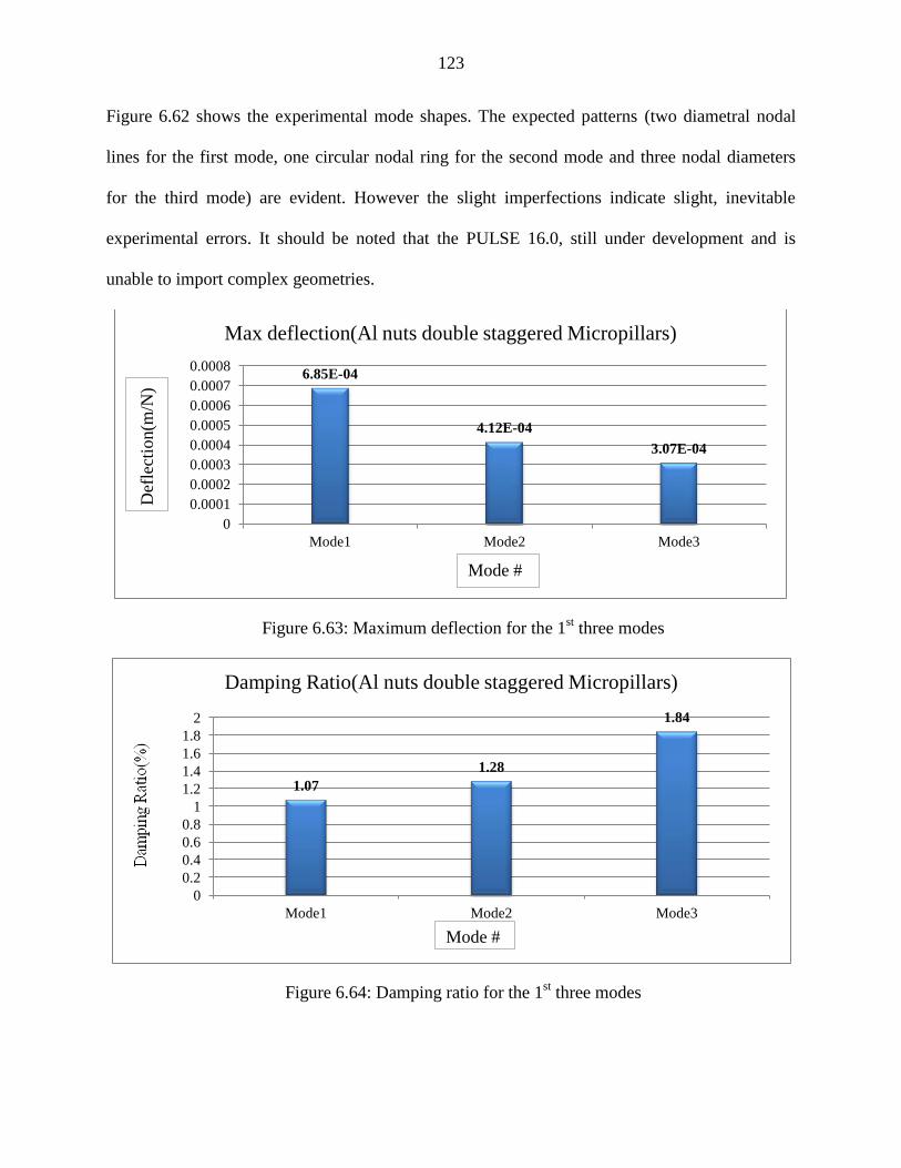
123
Figure 6.62 shows the experimental mode shapes. The expected patterns (two diametral nodal
lines for the first mode, one circular nodal ring for the second mode and three nodal diameters
for the third mode) are evident. However the slight imperfections indicate slight, inevitable
experimental errors. It should be noted that the PULSE 16.0, still under development and is
unable to import complex geometries.
Figure 6.63: Maximum deflection for the 1st three modes
Figure 6.64: Damping ratio for the 1st three modes
6.85E-04
4.12E-04
3.07E-04
0
0.0001
0.0002
0.0003
0.0004
0.0005
0.0006
0.0007
0.0008
Mode1 Mode2 Mode3
Max deflection(Al nuts double staggered Micropillars)
Def
lect
ion(m
/N)
Mode #
1.07
1.28
1.84
0
0.2
0.4
0.6
0.8
1
1.2
1.4
1.6
1.8
2
Mode1 Mode2 Mode3
Damping Ratio(Al nuts double staggered Micropillars)
Mode #

124
Figures 6.63 and 6.64 respectively show the maximum deflections and modal damping ratios for
the first three modes. It is obvious that mode one is the dominant mode with the largest
maximum deflection and the least modal damping. The maximum deflection decreases with
mode while the damping ratio increases with mode.
Table 6.7 compares the vibration results for the general periodic material group, and then these
results are shown in a graphical representation in order to give a better understanding about the
behavior of these structures. The number of peaks from experimental results is shown to indicate
modal densities of these samples over a specified frequency range.
Table 6.7: Vibration results for General periodic materials
Material Mode# Damping
ratio(η)%
Natural frequency(Hz)
Experimental
Max deflection(m/N) Number of
peaks(0-1.6kHz)
Micropillars
w/resonators
1 2.31 1095
3.20E-05 6
2 2.88 1673 9.22E-06
3 2.51 2001 1.41E-05
AL Nut
double
Staggered
MP*
1 1.07 650 6.85E-04 13
2 1.28 692 4.12E-04
3 1.84 754 3.07E-04
AL Nut
double in
line MP
1 0.58 572 5.41E-04 10
2 0.64 683 4.36E-04
3 0.72 802 3.56E-04
*: Micropillars
Figure 6.65 to 6.68 shows the comparisons between the different samples of the PCMS materials
as follows:
Figure 6.65: Comparison between natural frequencies for the 1st three modes.
Figure 6.66: Comparison between maximum deflections for the 1st three modes.
Figure 6.67: Comparison between damping ratios for the 1st three modes.
Figure 6.68: Comparison between modal densities.

125
Figure 6.65: Comparison between natural frequencies for the 1st three modes
As it can be seen from figure 6.65 that micropillars with resonators has the maximum natural
frequency for the first three modes among the group and this is due to its higher stiffness
compared with the other two constructions which look to be approximately the same. The other
two samples have much lower frequencies and almost the same because of their similarity of
design.
mode1
mode2
mode3
0
500
1000
1500
2000
2500
Micropillars
w/Resonators AL Nuts
DoubleStaggered
MP AL Nuts Double
in-line MP
mode1
mode2
mode3 Fre
quen
cy(H
z)
Material
Comparison between natural frequencies( Peroidic materials)

126
Figure 6.66: Comparison between maximum deflections for the 1st three modes
Figure 6.67: Comparison between damping ratios for the 1st three modes
mode1
mode2
mode3
0.00E+00
2.00E-04
4.00E-04
6.00E-04
8.00E-04
AL Nuts
DoubleStaggered
MP
AL Nuts Double
in-line MP Micropillars
w/Resonators
mode1
mode2
mode3
Max
Def
lect
ion(m
/N)
Material
Comparison between max deflection( Periodic materails)
mode1
mode2
mode3
0
1
2
3
Micropillars
w/Resonators AL Nuts
DoubleStaggered
MP AL Nuts Double in-
line MP
mode1
mode2
mode3
Dam
pin
g R
atio
(%)
Material
Comparison between damping ratios(Periodic materials)

127
Figures 6.66 and 6.67 respectively shows again that the micropillars with resonator material has
the minimum deflection and the maximum damping and this is totally correct as the design of
this material which contains these small resonators contribute in absorbing much of the vibration
energy which leads to minimum deflection and higher damping. As mentioned before the
behavior of this material is of much importance to be studied in the future as a meta material.
Figure 6.68: Comparison between modal densities
For the modal density (figure 6.68), it can be seen that the structures are complex because we
have this number of peaks in a short frequency band, the aluminum nut double staggered
micropillars seems to be the most complex among the group.
6.4. PARAMETRIC STUDIES
6.4.1 PARAMETRIC STUDIS FOR SOUND ABSORPTION COEFFICIENT
Parametric studies are normally used to see the effect of changing several parameters on the
outcome of any engineering investigation because this will save money and time and give
engineers the ability to decide which design should give the optimum results.
6
13
10
0
2
4
6
8
10
12
14
Micropillars w/resonators AL Nut double Staggered MP AL Nut double in line MP
Modal density(general periodic materials,0-1.6kHz)
# o
f pea
ks
Material

128
In the acoustic area the parametric study was done through writing a Matlab program -which
can be found in appendix A at the end of this dissertation -depending on Biot theory discussed
earlier in chapter three to calculate the sound absorption coefficient of rigid porous materials to
see the effect of different parameters on the absorption coefficient. The material selected was
Basalt because it was convenient for us to get its microscopic results from [84] thus saving much
time. To verify our computer program, the experimental result was compared with the program
result to show compatibility between them. After that the parameters were changed and the
results were graphically presented to give an indication of these changes on the sound absorption
coefficient.
As mentioned before the material was Basalt with the following properties:
Density: 3000 kg/m2
Thickness: 1 inch
Structure factor Ks: 3
Porosity: 0.1
Diameter of pore: 0.07 mm
Figure 6.69 shows the compatibility between the experimental and computer program results and
it is very good, the slight deviation only underscores the fact that experimental errors inevitable
in such an exercise. This benchmark comparison is the logical starting point for a parametric
study. This means that we can rely on the results of our parametric exercise since there is closer
agreement between the experimental and the computer code results for the same material and
conditions. Upon this result we started to change the thickness, porosity and finally structure
factor to see the effect of those parameters on the sound absorption.
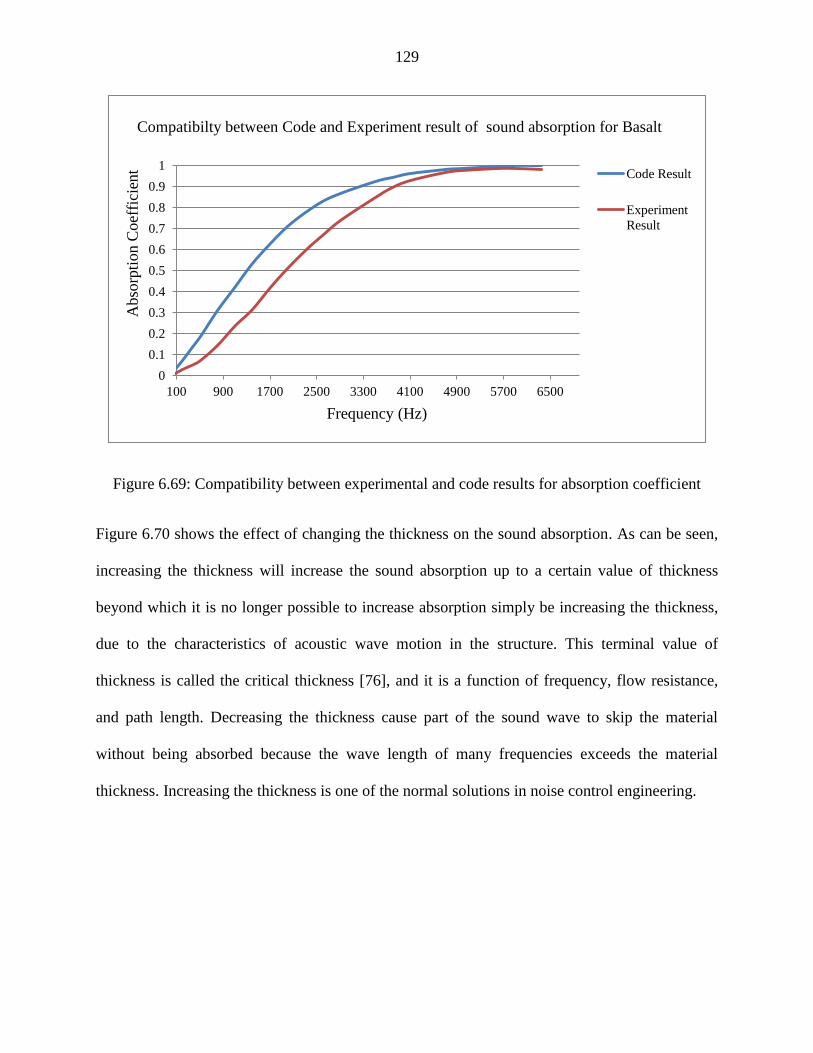
129
Figure 6.69: Compatibility between experimental and code results for absorption coefficient
Figure 6.70 shows the effect of changing the thickness on the sound absorption. As can be seen,
increasing the thickness will increase the sound absorption up to a certain value of thickness
beyond which it is no longer possible to increase absorption simply be increasing the thickness,
due to the characteristics of acoustic wave motion in the structure. This terminal value of
thickness is called the critical thickness [76], and it is a function of frequency, flow resistance,
and path length. Decreasing the thickness cause part of the sound wave to skip the material
without being absorbed because the wave length of many frequencies exceeds the material
thickness. Increasing the thickness is one of the normal solutions in noise control engineering.
0
0.1
0.2
0.3
0.4
0.5
0.6
0.7
0.8
0.9
1
100 900 1700 2500 3300 4100 4900 5700 6500
Code Result
Experiment
Result
Abso
rpti
on C
oef
fici
ent
Frequency (Hz)
Compatibilty between Code and Experiment result of sound absorption for Basalt

130
Figure 6.70: Effect of changing thickness on sound absorption
The second parameter which was changed is the porosity which is the volume of air inside the
material to the total volume of the material plus air. As can be seen from figure 6.71 that
increasing the porosity increases the sound absorption in the low frequency range. For example
as the porosity increases from 0.3 to 0.7, the peak of sound absorption is shifted to lower and
lower frequencies which is good if the material is to be used to absorb sound in the low
frequency area. Sound absorption is mainly due to two factors, viscous friction between the fluid
and the solid material and, the thermal effect between the two. In this case the viscous effect in
the low frequency range and higher porosity significantly increases. The thermal effect in the
same case similarly increases because there is more contact area. However in the high frequency
range the sound wave amplitude and wave length are much shorter and at high porosity (meaning
less material), both viscous and thermal effects are lower because there is less solid-fluid contact.
0
0.1
0.2
0.3
0.4
0.5
0.6
0.7
0.8
0.9
1
0 1000 2000 3000 4000 5000 6000 7000
t=1
t=0.8
t=0.75
t=0.5
0.25t
Ab
sorp
tio
n C
oef
fici
ent
Frequency (Hz)
Parametric Study shows the effect of Basalt thickness on sound absorption(t=1")

131
Figure 6.71: the effect of porosity on sound absorption coefficient
Finally the effect of structure factor (figure 6.72) which is the ratio between the length of all
pores (the non straight and straight pores) to the length of the straight pores is studied. In this
definition straight means parallel to the main flow direction. The value is typically between 3 and
7 in real life [46] situations. The influence of structure factor is straight forward in that this
quantity is used to multiply the fluid density in order to obtain an effective density that is used in
the flow equations for the sound absorption. The curves shown in the graph indicate how this
modification of density affects the calculated acoustic absorption coefficient. It may be observed
that at the frequency extremes the effect of increasing structure factor is negligible for a given
porosity value. In these zones the absorption coefficient already attains the values of almost zero
and almost one (the minimum and maximum possible) respectively. In the middle frequency
region the increase in absorption coefficient goes up to 0.25( at about 2000 Hz).
0
0.1
0.2
0.3
0.4
0.5
0.6
0.7
0.8
0.9
1
0 1000 2000 3000 4000 5000 6000 7000
0.1 porosity
0.3porosity
0.5 porosity
0.7 porosity
Parametric study shows the effect of porosity on sound absorption for Basalt A
bso
rpti
on C
oef
fici
ent
Frequency(Hz)

132
Figure 6.72: the effect of structure factor on sound absorption coefficient
6.4.2 PARAMETRIC STUDIES FOR VIBRATION
The parametric studies for vibration were done to see the effect on natural frequencies, of
changing thickness, architecture or layup (Lexan samples), dimensions and finally the origin
coordinates of cutting the PCMS circular samples from larger rectangular stock. This last
variable was studied to show the importance of choosing very precise coordinates for cutting
arbitrary shape samples from usually rectangular stock materials to avoid any variation in the
vibration behavior of these structures.
The single layer solid Lexan monolithic sample was selected to see the effect of changing
the thickness on the natural frequencies, the simulations were done using Abaqus standard 3D as
a solver in the FEM model, the thicknesses selected were (2, 4, 6, 8, and 10 mm). As mentioned
in the acoustic parametric study, the first step was to check the compatibility between
experimental and finite element results for this sample, the results are shown in figure 6.73
below for the 2mm sample and they show very good agreement.
0
0.1
0.2
0.3
0.4
0.5
0.6
0.7
0.8
0.9
1
0 1000 2000 3000 4000 5000 6000 7000
Ks=1
Ks=2
Ks=3
Ks=5
Ks=7
Parametric study shows the effect of structure factor on sound absorption for Basalt A
bso
rpti
on C
oef
fici
ent
Frequency(Hz)

133
Figure 6.73: Compatibility between experimental and FEM results for natural frequencies
As can be seen from the graph, increasing the thickness increases the natural frequency for each
of the first three modes. This is reasonable because increasing the thickness will make the
material stiffer, and the effect of this stiffness increase exceeds that of the mass increase, and
since frequency is the square root of the ratio of effective stiffness to effective mass, the natural
frequency will increase.
Figure 6.74: effect of thickness on natural frequency
250 300 350 400 450 500 550 600 650 700 750
mode1 mode2 mode3
finite element
experiment F
requen
cy(H
z)
Mode #
Compatibilty between FEM and experiment(1 layer Lexan solid)
313
560 821 1088 1344
563
1004
1470
1940
2384
728
1293
1876
2453
2986
0
1000
2000
3000
4000
5000
6000
7000
8000
2mm 4mm 6mm 8mm 10mm
ωn3
ωn2
ωn1
Parametric Study of the effect of material thickness on the 1st three natural frequencies(Lexan
solid, FEM results)
Materail Thickness
Fre
quen
cy(H
z)

134
The second parametric study was done to see the effect of changing the architecture of single
layer Lexan material on the natural frequency behavior, the samples used were:
1. Single layer solid Lexan
2. Single layer Lexan with small holes
3. Single layer Lexan with large holes
4. Single layer Lexan with membrane
Figure 6.75 shows the results. As can be seen, the natural frequency decreases as more material
is removed from the solid Lexan disk. It can also be seen that going from the solid disk to one
with small holes(5mm diameter) covered with the silicon membrane and to the one with small
holes results in rather small decrements of frequency, but removing large holes (13mm diameter)
results in a steep drop in natural frequency. Again, this is reasonable because removing material
decreases stiffness, and the effect of this stiffness decrease exceeds that of the mass decrease,
and since frequency is the square root of the ratio of effective stiffness to effective mass, the
natural frequency will decrease. The observed discrepancy in the frequency decrease over the
four structures can be readily attributed to the fact that much more material (2.01e-5 m3) is
removed than for the case of small holes (3.29e-6 m3). The membrane adds only a little mass (it
is 0.2mm thickness).

135
Figure 6.75: Fundamental natural frequency for different architecture
The finite element results were as shown in table 6.8 below.
Table 6.8: the first three resonance frequencies for different Lexan architecture
Material Mode1 Mode2 Mode3
f1 f2 f3
1Layer Solid 322 574 746
1 Layer w/small holes 313 559 728
1 Layer w/large holes 269 411 624
1 Layer w/membrane 318 563 736
The effect of sample dimension was studied for PCMS aluminum prismatic rectangular plate, the
plate dimensions were as follows:
1. Sample 1, 62.2cm x62.2cm x 4cm, (24.5in. x24.5in. x1.57in.)
2. Sample 2, 15.2 cm. x15.2 cm. x 4cm.,(6in. x6in. x 1.57in.)
269
313 318
322
250
260
270
280
290
300
310
320
330
1 Layer w/large
holes
1 Layer w/small
holes
1 Layer
w/membrane
1Layer Solid
First natural frequency shift(FEM results)
Fre
qu
ency
(Hz)
Material

136
Figures 6.76 and 6.77 show the results for the displacement contour for samples 1 and 2
respectively.
Mode1 Mode2 Mode3
Figure 6.76: displacement contour for sample 1
Mode1 Mode2 Mode3
Figure 6.77: displacement contour for sample2
Table 6.9 shows the natural frequencies and VonMises stresses for the first three modes for both
samples. It is obvious that the frequencies for sample1 are much lower than those for sample2 ,
this is due to the fact that as the dimensions increase the structure becomes less stiff and heavier
which directly affect the natural frequencies. The maximum deflections are also higher for the
larger structure resulting in an increase in VonMises stresses. The mode shapes are clearer for
the larger sample (it conforms to the established mode shapes of rectangular plates), and this is
due to the fact that there is no mid-structure free edges like those found in the smaller sample.
These mid- structure free edges or hanging lips arose from extracting the small sample size from
the larger size stock material. Such a hanging lip vibrates wildly on its own and distorts the
normal rectangular mode shape.

137
Table 6.9: natural frequencies and VonMises stress for the CMI samples
Sample
number
Dimensions(cm)
L*W*H
Mode1 Mode2 Mode3
f1*
σ1**
f2 σ2 f3 σ3
1 62.2*62.2*4 386 1.49e5 589 1.81e5 757 1.75e5
2 15.2*15.2*4 4369 405 6487 450 7526 375
*: frequency in hertz **: VonMises Stress in Mpa
The last parametric study was done on different cuts of circular samples (100 mm diameter) from
the rectangular aluminum and stainless steel PCMS block materials. The cuts were made
digitally using the Unigraphics software. The aluminum samples were classified according to the
gap (the distance between the lower extremity of the hanging lip and the top of the lower skin) as
shown in figure 6.78 below. Each cut corresponds to a different location of the center of the
100mm circle. The variation between all these centers was no more than 2mm.
Figure 6.78: Gaps for two different aluminum samples

138
We have seven different cuts for the aluminum sample. Our sample is part 4 with 3.825mm gap.
The center point used to extract this part corresponds to the original location. Each other part was
obtained by shifting this center to a different position. In no case was this shift more than 2mm.
The results for these samples are shown in table 6.10
Table 6.10: Results for different samples from FEM simulations for aluminum samples Part # Gap(mm) Von Mises Stress(Mpa)
Natural Frequency(Hz)
Mode1 Mode2 Mode3 f1 f2 f3
1 8.418 601 2140 1620 9760 11518 12735
2 11.053 624 2120 1280 10244 11602 12814
3 15.34 697 1870 1190 10810 11666 12867
4 3.825 621 2000 941 8997 11314 12364
5 13.608 631 1830 1160 10632 11650 12855
6 12.742 642 1870 1190 10483 11627 12794
7 7.475 626 1400 1060 9570 11478 12680
8 16.249 782 1920 1200 10828 11660 12809
Figure 6.79: The change of frequency with gap
8997
9570 9760
10244
10483 10632
10810 10828
8500
9000
9500
10000
10500
11000
3.825mm 7.475mm 8.418mm 11.053mm 12.742mm 13.608mm 15.34mm 16.249mm
Gap (mm)
Fre
quen
cy(H
z)
Effect of Gap on the first natural frequency for Aluminum prismatic Microtruss,
PCMS

139
Figure 6.80: Change of VonMises stress with gap
Figure 6.79 and 6.80 show the natural frequencies and VonMises stresses respectively for the
differtent cuts. The results are arranged in an acending order of the gap described earilier. Figure
6.79 shows the monotonic increase in natural frequency for increasing gap distance. This is
logical because as more materail is progressively removed the remainimg structure becomes
more compact and stiffer for relatively little change in mass. This results in frequency increase.
On the other hand the VonMises stress which is an indication of the avearge stress shows a
somewhat arbitrary behavior. This also understandable because the deflection allover the
structure also becomes arbitrarly distributed. The mode shapes for the different samples are
shown in figure 6.81 below.
621 626
601 624
642 631
697
782
550
600
650
700
750
800
3.825mm 7.475mm 8.418mm 11.053mm 12.742mm 13.608mm 15.34mm 16.249mm
Von Mises stress change with gap for the first mode(Aluminum prismatic Micro truss, PCMS) S
tres
s(M
pa)
Gap (mm)

140
VonMises Stress Contour Displacement Contour
Mode1 Mode2 Mode3 Mode1 Mode2 Mode3
Figure 6.81: VonMises and displacement contours for Aluminum prismatic PCMS cuts arranged
according to table 6.10
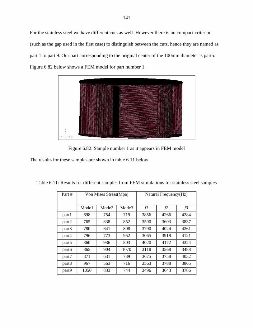
141
For the stainless steel we have different cuts as well. However there is no compact criterion
(such as the gap used in the first case) to distinguish between the cuts, hence they are named as
part 1 to part 9. Our part corresponding to the original center of the 100mm diameter is part5.
Figure 6.82 below shows a FEM model for part number 1.
Figure 6.82: Sample number 1 as it appears in FEM model
The results for these samples are shown in table 6.11 below.
Table 6.11: Results for different samples from FEM simulations for stainless steel samples
Part # Von Mises Stress(Mpa) Natural Frequency(Hz)
Mode1 Mode2 Mode3 f1 f2 f3
part1 698 754 719 3856 4266 4284
part2 765 838 852 3500 3603 3837
part3 780 641 808 3790 4024 4261
part4 796 773 952 3065 3918 4121
part5 860 936 803 4020 4172 4324
part6 865 904 1070 3118 3568 3488
part7 871 631 739 3675 3758 4032
part8 967 563 716 3563 3788 3865
part9 1050 833 744 3496 3643 3786

142
Figure 6.83: The first mode natural frequencies for stainless steel samples
Figure 6.84: The first mode VonMises stress for stainless steel samples
Figure 6.83 and 6.84 show the natural frequencies and VonMises stresses respectively for the
differtent cuts. The results are arranged in acenedning order of part number. The natural
frequencies don not follow any particular order . This is logical because the stainless steel
structure has numorous vertical plates which make up the triangular honeycomb core structure.
3563 3500
3675
3856
4020
3790
3496
3118 3065
3000
3200
3400
3600
3800
4000
4200
part1 part2 part3 part4 part5 part6 part7 part8 part9
Natural Frequency(Mode1 Stainless steel samples)
Fre
qu
ency
(Hz)
Part #
967
765
871
698
860 780
1050
865 796
0
200
400
600
800
1000
1200
part1 part2 part3 part4 part5 part6 part7 part8 part9
VonMises Stress(Mode1,stainless steel samples)
Str
ess(
Mpa)
Part #

143
Any slight shift in the coordinate of the center of the circular part to the cut makes a big
differrence in the vibration behavior because some of these vertical panels may now become
loose. The VonMises stress which is an indication of the avearge stress also shows arbitrary
behavior. This also understandable because the deflection allover the structure also becomes
arbitrarly distributed.
The mode shapes for both dispalcement and VonMises stess contours is shown in figure 6.85
below to give an imperssion about the complexity of these samples.

144
VonMises contour Displacement contour
Mode2 Mode2 Mode3 Mode1 Mode2 Mode3
Figure 6.85: VonMises and displacement contours for stainless steel triangular honeycomb
PCMS cuts arranged according to table 6.16

145
The behavior of the cuts from these two periodic materilas brings a very important observation to
the forefront. They show that it is crucial to insure that when replictae parts are required, they
must be extracted from an exact geometrical location, otherwise it will be impossible to assure
consistency in the vibration and stress behaviores of the structures so produced. This has severe
production and financial implications.
Inorder to underscore this point, table 6.12 shows a variation of a mere 2mm in the center
location of the cut leads to varations of 20% for mode 1 frequency and 29% for mode 1 avearge
stress for the aluminum sample and 23% for mode 1 frequency and 41% for mode 1 avearge
stress for the stainless steel sample.
Table 6.12: perentage varaitions for the (frequency and strees)from the original sample
Material Deviation from original location results%
Mode1 Mode2 Mode3
f σ* f σ f σ
Aluminum prismatic Microtruss 20 29 3 37 4 72
Stainless steel triangular honeycomb
Microtruss
23 41 16.7 39 19.3 41
*: VonMises stress

146
CHAPTER 7
CONCLUSIONS AND FUTURE WORK
7.1 CONCLUSIONS
The work reported in this dissertation has covered six groups of vibro-acoustic containment
materials that are presently or potentially useful in the automotive area. These are the fabric,
foam, honeycomb, monolithic and sandwich, periodic cellular material structures and general
periodic groups. The first two were examined for acoustic containment only, while the remaining
four groups were examined for both vibration and acoustic reduction applications.
There are important novel points in the research –
(a) PCMS: Investigation of the vibro-acoustic responses of periodic cellular material
structures for possible use in the abatement of noise and vibration. This class of materials had
been examined for structural, heat-transfer and multi-functional deployment, but not for the
present purposes. From the results, we may conclude that the acoustic performance of this group
of materials is unsatisfactory. They will need to be supplemented with good acoustic absorbers.
Examples are filling with acoustic foam, or resinated cotton wrapped with very thin plastic to fill
the cavities. On the other hand, a honeycomb plate can be attached on one face. It should be
remembered that the construction can be modified to improve damping and acoustic absorption,
e.g. by including many bars that basically rub against one another when flexed, or including the
equivalent of air gaps.
(b) Construction and testing of novel generally periodic structures: Three novel designs of
these materials (micro-pillars with resonators, aluminum double staggered micro-pillars, and
aluminum double in-line micro-pillars) were made. These materials have the capability of being

147
utilized as acoustic meta-materials when design tuning is used to proportion their parts to
produce negative effective mass and negative effective stiffness with the potential that acoustic
and vibration band gaps of frequency could be created.
(c) Lexan vibro-acoustics: although Lexan (GE polycarbonate) is a commercially important
industrial material world-wide, investigation of possible different ways of vibro-acoustic
applications are sparse. This research has tested Lexan material samples in different formations
to elicit behavior in some varying configurations. The results show that, in normal thicknesses,
Lexan material is a bad absorber but a good reflector of sound; therefore it will perform well as a
sound barrier material and as a suspended acoustic panel which can be set into vibration by
incident sound pressure wave. Thick Lexan can be used as sound deadening partitions or
enclosures. Because of good impact properties, laminated Lexan can be used as bullet-proof
partitions in military cars and security applications.
(d) Programs and codes: A Matlab computer program was written to calculate the acoustic
absorption of fibrous materials, and utilized to compute and plot values over the frequency range.
Secondly, for some PCMS materials, finite element (RADIOSS) computational programs were
completely set up for the calculation of vibration results based on several input parameter sets
including geometry variations, etc., but could not be fully calculated owing to computational
resources. The numbers of nodes required could not be accommodated in the WSU license
available to students. Since the computational infrastructure work is done, all that remains is the
acquisition of faster, higher capacity, possibly parallel-architecture computing platform to
execute the programs.
(e) Parametric studies: four such studies have been carried out in this work. These were
respectively on the acoustic absorption properties of rigid frame porous materials; on Lexan
148
architectural simulations; on size effect in rectangular PCMS samples; and on effects of tiny
variations in the extraction location of smaller samples from general PCMS block-type stock
materials for two different PCMS samples.
The major findings of this research are that
1. Fabric materials generally have high absorption coefficients. (Thus useful as filler /
addition in synthesized panel materials to improve acoustics).
2. The B&K polyethylene terephthalate (PET) is a good broadband acoustic absorber.
Conclusions on the Kathawate Inc. magic foam materials must wait until there is certainty about
their manufacturing (oven expansion) methods from raw stock.
3. Acoustic absorption coefficients of honeycomb, periodic materials are high in the mid-
frequency range (about 1500 Hz to 4100 Hz). As air contained in the cells is sealed in, and this
enables the incident sound to be destructively reflected multiples of times. However, the
particular choices of honeycomb to be used or in combination must be carefully made depending
on frequencies to be covered.
4. Acoustic absorption coefficients of monolithic and sandwich materials tend to manifest
single or only a few peaks, hence limited frequencies are covered, the sandwich materials may
not be useful as general absorbers unless some of the component materials are highly absorbent.
5. Replacing some of the absorber material with air (e.g. by drilling holes) or membrane
tends to improve flexibility and absorption. It is also confirmed that increasing air gaps in
absorber arrangements tends to significantly improve absorption in the low frequency range and
slightly deteriorate it at higher frequencies.

149
6. More rigid materials, such as cold rolled steel and block aluminum, as well as stiff
framed structures, even in combination with highly absorbent cores or layers, tend to limit
vibration, and should be considered for this purpose in automotives wherever a weight penalty
does not work against them.
7. Potential exists for PCMS and generally periodic structures to offer effective vibration
control. They may be used in ways mentioned in section (7.1a) and(4.1.6).
7.2 FUTURE WORK
Four areas are seen from this research to merit future work, as they directly grow from the
present investigation.
1. Actual panels: It is necessary to next test a few actual automotive panels that are treated
with the materials adjudged best from this work. Since the test samples are of the same size, the
present findings are totally valid. However, on account of the size effect, such a scale-up is
needful.
2. Further analysis and code development: Analytical and computer program development
should be performed for other classes of materials in order to foster a wider view of possibilities
and how they compare.
3. Computing resources: It is essential to expand the computing resources which are
presently available, such that the computation schemes which are already set up may be executed
for more parametric studies, and others may also be implemented.
4. Meta-materials: Analysis and computer simulations relating to general periodic materials
should be undertaken, as there is great economic benefit in using the band-gap approach to avoid

150
signal transmission in certain frequency ranges rather than containing them when they are
already transmitted.

151
APPENDEX A
MATLAB CODE TO CALCULATE SOUND ABSORPTION COEFFICIENT FOR
POROUS RIGID MATERIALS.
%This program is written to calculate sound absorption coefficient for rigid
fram porous materials according to Biot theory using Matlab. function case1()
%The frequency is changed from 0 to 6.4 kHz with an increment of 2
%FREQ is frequency in Hertz; ω is radial frequency in rad per second
%RA is the real part of impedance
%RI is the imaginary part of impedance
%C is the sound velocity (mm/sec)
%RHO is the density of Air (g/mm3)
%ETHA is the viscosity of Air (g/mm.sec)
%ABSO is the sound absorption coefficient
ETHA=1.8E-5; C=3.4E5; RHO=1.21765E-6; l=440;
t = input('Thickness: '); d= input('Diameter of pores: '); p=input('Porosity: '); KS = input('Structure Factor: ');
disp('Thickness= '); disp(t) disp('Diameter of pores = '); disp(d) disp('Porosity= '); disp(p) disp('Structure Factor= '); disp(KS) FREQ=50; i=0; for FREQ=50:FREQ+2:6400 R=32.0*ETHA/(d*d*t); w=2.0*pi*FREQ; THETA=atan(-R/(KS*RHO*w)); K1=sqrt(KS+(R/RHO/w)*(R/RHO/w)); RHO1=(RHO*C/sqrt(p)); p1=w/(C*sqrt(p)); s1=sin(THETA/2.0); c1=cos(THETA/2.0); A=s1*p1*K1; B=c1*p1*K1; HTA=tanh(-A); TB=tan(B);
RA=(RHO1*K1*c1*(HTA+HTA*TB*TB)+RHO1*K1*s1*(TB-HTA*HTA*TB))/(HTA*HTA+TB*TB); XA=(RHO1*K1*s1*(HTA+HTA*TB*TB)-RHO1*K1*s1*(TB-HTA*HTA*TB))/(HTA*HTA+TB*TB); k=C/FREQ;
RSIMPE=RA/((cos(k*l)+XA*sin(k*l))*(cos(k*l)+XA*sin(k*l))+
RA*sin(k*l)*RA*sin(k*l)); ISIMPE=((sin(k*l)-XA*cos(k*l))*(cos(k*l)+XA*sin(k*l))-
RA*RA*cos(k*l)*sin(k*l))/((cos(k*l)+XA*sin(k*l))*(cos(k*l)+XA*sin(k*l))+RA*si
n(k*l)*RA*sin(k*l));

152
ABSO=4.0*RSIMPE/((1.0+RSIMPE)*(1.0+RSIMPE)+ISIMPE*ISIMPE); i=i+1; FREQarray(i) = FREQ; ABSOarray(i) = ABSO; disp('FREQ = ');disp(FREQ); disp(' ');disp('ABSO= ');disp(ABSO) end
plot(FREQarray,ABSOarray,'-
gd','LineWidth',2,'MarkerEdgeColor','k','MarkerFaceColor','y','MarkerSize',2) title('FREG vs ABSO') xlabel('FREQ','FontSize',12); ylabel('ABSO','FontSize',12) grid on

153
APPENDIX B
MATLAB CODE TO CALCULATE NATURAL FREQUENCIES AND MODE SHAPES
FOR LEXAN The following is a program written in Matlab using vibration toolbox
[Reference 71] to calculate the natural frequencies and mode shapes for
single layer solid Lexan.
>> rou= 2.64; E=2350e6; mu=0.375;
>> a=50e-3; h=2.2e-3;
>> Plate_Pars=[rou E mu a h];
>> cirplate(Plate_Pars,0)
System Information
------------------
Material Properties:
Mass density (mass/area) rou = 2.64
Young's modulus E = 2350000000
Poisson's ratio mu = 0.375
Geometric Properties:
Radius a = 0.05
Thickness h = 0.0022
Bending stiffness D = E*h^3/(1-mu^2)/12 = 2.4265
c = sqrt(D/rou) = 0.9587
Boundary Conditions:
Free edge at r = a: Mr = 0, Vr = Qr + 1/r*(Mrs,s), where s = theta
Natural Frequencies:
-------------------
w_mn n = 0 1 2 3 4
------------------------------------------------------------
m =
1.0e+005 *
0 0 0 0.0208 0.0478 0.0836
0.0000 0.0351 0.0789 0.1351 0.2025 0.2805
0.0000 0.1480 0.2298 0.3236 0.4289 0.5452
0.0000 0.3371 0.4567 0.5881 0.7311 0.8853
0.0000 0.6020 0.7593 0.9285 1.1091 1.3012
Here w_mn = natural frequency in rad/s
m = number of nodal circles
n = number of nodal diameters
* Note: The membrane has rigid-body modes (zero eigenvalues)
Mode Shapes

154
-----------
Wmn(r, theta) = [Jn(g_mn*r) + d_mn*In(g_mn*r)]*cos(n*theta), 0<=r<=a,
0<=theta<=2*pi
Here Jn = Bessel function of the first kind
In = Bessel function of the second kind
g_mn = frequency parameters, w_mn = g_mn^2* sqrt(D/rou)
d_mn = constants of mode shapes
g_mn n = 0 1 2 3 4
------------------------------------------------------------
m =
0 0 0 46.5482 70.6291 93.3573
1.0000 60.5463 90.7083 118.6883 145.3275 171.0621
2.0000 124.2600 154.8284 183.7288 211.5117 238.4783
3.0000 187.5161 218.2518 247.6797 276.1513 303.8847
4.0000 250.5772 281.4279 311.1992 340.1361 368.4035
d_mn n = 0 1 2 3 4
------------------------------------------------------------
m =
0 0 0 0.2306 0.1009 0.0483
1.0000 -0.0811 -0.0187 -0.0055 -0.0019 -0.0007
2.0000 0.0031 0.0007 0.0002 0.0001 0.0000
3.0000 -0.0001 -0.0000 -0.0000 -0.0000 -0.0000
4.0000 0.0000 0.0000 0.0000 0.0000 0.0000
Non-dimensional Frequency Parameters, z_mn = g_mn*a
----------------------------------------------------
z_mn n = 0 1 2 3 4
------------------------------------------------------------
m =
0 0 0 2.3274 3.5315 4.6679
1.0000 3.0273 4.5354 5.9344 7.2664 8.5531
2.0000 6.2130 7.7414 9.1864 10.5756 11.9239
3.0000 9.3758 10.9126 12.3840 13.8076 15.1942
4.0000 12.5289 14.0714 15.5600 17.0068 18.4202
To plot mode shape W_mn, use function PLOTMSH4(m,n)
To animade mode (m,n), use function ANIMODE4(m,n)
PLOTMSH4(0,2), Mode 1
Spatial Distribution of Mode (0,2)
-----------------------------------
Number of nodal circles m = 0
Number of nodal diameters n = 2
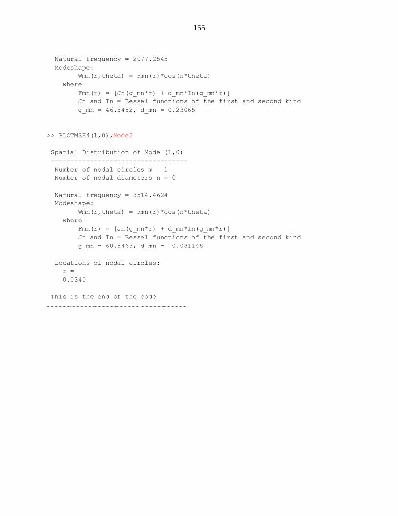
155
Natural frequency = 2077.2545
Modeshape:
Wmn(r,theta) = Fmn(r)*cos(n*theta)
where
Fmn(r) = [Jn(g_mn*r) + d_mn*In(g_mn*r)]
Jn and In = Bessel functions of the first and second kind
g_mn = 46.5482, d_mn = 0.23065
>> PLOTMSH4(1,0),Mode2
Spatial Distribution of Mode (1,0)
-----------------------------------
Number of nodal circles m = 1
Number of nodal diameters n = 0
Natural frequency = 3514.4624
Modeshape:
Wmn(r,theta) = Fmn(r)*cos(n*theta)
where
Fmn(r) = [Jn(g_mn*r) + d_mn*In(g_mn*r)]
Jn and In = Bessel functions of the first and second kind
g_mn = 60.5463, d_mn = -0.081148
Locations of nodal circles:
r =
0.0340
This is the end of the code
………………………………………………………………………………………………
156
APPENDIX C
EGIN VALUE OUTPUT FOR ONE LAYER LEXAN WITH LARGE HOLES
Abaqus 6.9-2 Date 06-Feb-2012 Time 21:58:54
For use at Wayne State University under license from Dassault Systemes or its
subsidiary.
The Abaqus Software is a product of:
Dassault Systemes Simulia Corp.
Rising Sun Mills
166 Valley Street
Providence, RI 02909-2499, USA
Available for internal use at Wayne State University.
The Abaqus Online Support System is accessible
through the "My Support" section of the SIMULIA
Home Page at http://www.simulia.com.
Support policies for academic licenses are described
on the SIMULIA web site at
http://www.simulia.com/academics/academic_support.html.
On machine lan1.grid.wayne.edu
you are authorized to run
Abaqus/Standard until 04-Oct-2012
Your site id is: 08WAYNEUA
For assistance or any other information you may
obtain contact information for your local office
from the world wide web at:
http://www.simulia.com/about/locations.html
* * * * * * * * * * * * * * * * * * * * * * * * * * * * * *
* *
* ***************** *
* * N O T I C E * *
* ***************** *
* *
* *
* Abaqus 6.9-2 *
* *
* BUILD ID: 2009_07_10-10.30.58 92676 *
* *
* *
* Please make sure you are using release 6.9 manuals *
* plus the notes accompanying this release. *
* *
* *
* *
* *
* *
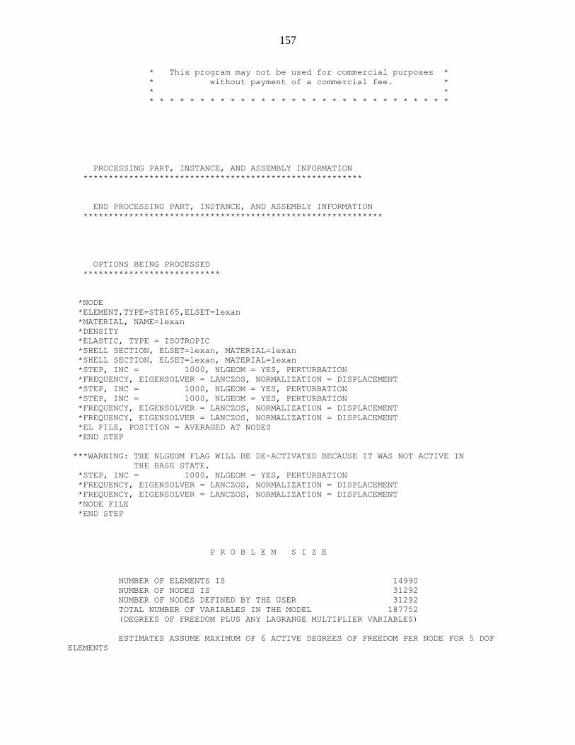
157
* This program may not be used for commercial purposes *
* without payment of a commercial fee. *
* *
* * * * * * * * * * * * * * * * * * * * * * * * * * * * * *
PROCESSING PART, INSTANCE, AND ASSEMBLY INFORMATION
*******************************************************
END PROCESSING PART, INSTANCE, AND ASSEMBLY INFORMATION
***********************************************************
OPTIONS BEING PROCESSED
***************************
*NODE
*ELEMENT,TYPE=STRI65,ELSET=lexan
*MATERIAL, NAME=lexan
*DENSITY
*ELASTIC, TYPE = ISOTROPIC
*SHELL SECTION, ELSET=lexan, MATERIAL=lexan
*SHELL SECTION, ELSET=lexan, MATERIAL=lexan
*STEP, INC = 1000, NLGEOM = YES, PERTURBATION
*FREQUENCY, EIGENSOLVER = LANCZOS, NORMALIZATION = DISPLACEMENT
*STEP, INC = 1000, NLGEOM = YES, PERTURBATION
*STEP, INC = 1000, NLGEOM = YES, PERTURBATION
*FREQUENCY, EIGENSOLVER = LANCZOS, NORMALIZATION = DISPLACEMENT
*FREQUENCY, EIGENSOLVER = LANCZOS, NORMALIZATION = DISPLACEMENT
*EL FILE, POSITION = AVERAGED AT NODES
*END STEP
***WARNING: THE NLGEOM FLAG WILL BE DE-ACTIVATED BECAUSE IT WAS NOT ACTIVE IN
THE BASE STATE.
*STEP, INC = 1000, NLGEOM = YES, PERTURBATION
*FREQUENCY, EIGENSOLVER = LANCZOS, NORMALIZATION = DISPLACEMENT
*FREQUENCY, EIGENSOLVER = LANCZOS, NORMALIZATION = DISPLACEMENT
*NODE FILE
*END STEP
P R O B L E M S I Z E
NUMBER OF ELEMENTS IS 14990
NUMBER OF NODES IS 31292
NUMBER OF NODES DEFINED BY THE USER 31292
TOTAL NUMBER OF VARIABLES IN THE MODEL 187752
(DEGREES OF FREEDOM PLUS ANY LAGRANGE MULTIPLIER VARIABLES)
ESTIMATES ASSUME MAXIMUM OF 6 ACTIVE DEGREES OF FREEDOM PER NODE FOR 5 DOF
ELEMENTS

158
END OF USER INPUT PROCESSING
JOB TIME SUMMARY
USER TIME (SEC) = 2.6100
SYSTEM TIME (SEC) = 0.42000
TOTAL CPU TIME (SEC) = 3.0300
WALLCLOCK TIME (SEC) = 4
1
Abaqus 6.9-2 Date 06-Feb-2012 Time 21:59:01
For use at Wayne State University under license from Dassault Systemes or its
subsidiary.
STEP 1 INCREMENT 1
TIME COMPLETED IN THIS STEP 0.00
S T E P 1 C A L C U L A T I O N O F E I G E N V
A L U E S
F O R N A T U R A L F R E Q U E N C I
E S
THE LANCZOS EIGENSOLVER IS USED FOR THIS ANALYSIS
Abaqus WILL COMPUTE UNCOUPLED
STRUCTURAL AND ACOUSTIC MODES
NUMBER OF EIGENVALUES 15
HIGHEST FREQUENCY OF INTEREST 1.00000E+18
MAXIMUM NUMBER OF STEPS WITHIN RUN 35
BLOCK SIZE FOR LANCZOS PROCEDURE 7
THE EIGENVECTORS ARE SCALED SO THAT
THE LARGEST DISPLACEMENT ENTRY IN EACH VECTOR
IS UNITY
THIS IS A LINEAR PERTURBATION STEP.
ALL LOADS ARE DEFINED AS CHANGE IN LOAD TO THE REFERENCE STATE
TOTAL MASS OF MODEL
1.4737189E-05
LOCATION OF THE CENTER OF MASS OF THE MODEL
-5.0217554E-04 -3.5795413E-09 0.000000
MOMENTS OF INERTIA ABOUT THE ORIGIN
I(XX) I(YY) I(ZZ)
9.5235437E-03 1.0316722E-02 1.9833769E-02

159
PRODUCTS OF INERTIA ABOUT THE ORIGIN
I(XY) I(XZ) I(YZ)
-3.4137204E-13 0.000000 0.000000
MOMENTS OF INERTIA ABOUT THE CENTER OF MASS
I(XX) I(YY) I(ZZ)
9.5235437E-03 1.0316722E-02 1.9833769E-02
PRODUCTS OF INERTIA ABOUT THE CENTER OF MASS
I(XY) I(XZ) I(YZ)
-3.4134555E-13 0.000000 0.000000
M E M O R Y E S T I M A T E
PROCESS FLOATING PT MINIMUM MEMORY MEMORY TO
OPERATIONS REQUIRED MINIMIZE I/O
PER ITERATION (MBYTES) (MBYTES)
1 4.46E+09 100 1319
E I G E N V A L U E O U T P U T
MODE NO EIGENVALUE FREQUENCY GENERALIZED MASS COMPOSITE
MODAL DAMPING
(RAD/TIME) (CYCLES/TIME)
1 -3.62916E-05 0.0000 0.0000 4.00201E-06 0.0000
2 -1.83950E-05 0.0000 0.0000 1.19590E-05 0.0000
3 -5.47595E-06 0.0000 0.0000 1.08393E-05 0.0000
4 3.28435E-05 5.73093E-03 9.12106E-04 3.54520E-06 0.0000
5 3.60072E-05 6.00060E-03 9.55025E-04 6.73178E-06 0.0000
6 8.38131E-05 9.15495E-03 1.45706E-03 1.04820E-05 0.0000
7 2.90498E+06 1704.4 271.26 3.20951E-06 0.0000
8 3.08678E+06 1756.9 279.62 2.84219E-06 0.0000
9 6.97361E+06 2640.8 420.29 3.61025E-06 0.0000
10 1.61425E+07 4017.8 639.45 2.57056E-06 0.0000
11 1.68599E+07 4106.1 653.50 2.11985E-06 0.0000
12 3.63335E+07 6027.7 959.34 2.51842E-06 0.0000
13 3.67619E+07 6063.2 964.98 2.98243E-06 0.0000
14 5.03890E+07 7098.5 1129.8 1.83132E-06 0.0000
15 5.18386E+07 7199.9 1145.9 2.24029E-06 0.0000
THE ANALYSIS HAS BEEN COMPLETED
ANALYSIS COMPLETE
WITH 1 WARNING MESSAGES ON THE DAT FILE

160
JOB TIME SUMMARY
USER TIME (SEC) = 68.370
SYSTEM TIME (SEC) = 19.550
TOTAL CPU TIME (SEC) = 87.920
WALLCLOCK TIME (SEC) = 97

161
APPENDIX D
VIBRATION RESULTS FOR ONE MORE SAMPLE FROM EACH GROUP
DESCRIBED IN THE DISSERTATION WITH SAME SEQUENCE
1. Aluminum honeycomb
Figure D1: The stability diagram which indicates the first three natural frequencies
Figure D2: FRF, Coherence and phase
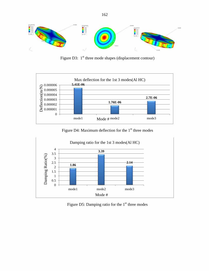
162
Figure D3: 1st three mode shapes (displacement contour)
Figure D4: Maximum deflection for the 1st three modes
Figure D5: Damping ratio for the 1st three modes
5.41E-06
1.76E-06
2.7E-06
0
0.000001
0.000002
0.000003
0.000004
0.000005
0.000006
mode1 mode2 mode3
Max deflection for the 1st 3 modes(Al HC)
Def
lect
ion
(m/N
)
Mode #
1.86
3.39
2.14
0
0.5
1
1.5
2
2.5
3
3.5
4
mode1 mode2 mode3
Damping ratio for the 1st 3 modes(Al HC)
Dam
pin
g R
atio
(%)
Mode #

163
Figure D6: Compatibility between experiment and FEM results
2. 1 layer solid Lexan
Figure D7: The stability diagram which indicates the first three natural frequencies
3547
5570 6209
3291
5262 5908
0
1000
2000
3000
4000
5000
6000
7000
Mode1 Mode2 Mode3
Experimental
Finite Element
Fre
qu
ency
(Hz)
Mode #
Compatibilty between Experiment and Finite Element(AL HC)

164
Figure D8: FRF, Coherence and phase
Figure D9: 1st three mode shapes (displacement contour)

165
Figure D10: 1st three mode shapes (displacement contour, Matlab)
Figure D11: Maximum deflection for the 1st three modes
1.67E-03
3.87E-04
6.19E-04
0.00E+00
2.00E-04
4.00E-04
6.00E-04
8.00E-04
1.00E-03
1.20E-03
1.40E-03
1.60E-03
1.80E-03
Mode1 Mode2 Mode3
Max deflection(1 Layer Solid Lexan)
Max
Def
lect
ion(m
/N)
Mode #

166
Figure D12: Damping ratio for the 1st three modes
Figure D13: Compatibility between experiment and FEM results
1.32
2.7
1.41
0
0.5
1
1.5
2
2.5
3
Mode1 Mode2 Mode3
Damping ratio(1 Layer solid lexan)
Dam
pin
g R
atio
(%)
Mode #
310
581
715
313
563
728
331
558
760
320
553
746
0
100
200
300
400
500
600
700
800
ωn1 ωn2 ωn3
Experiment
Finite Element
Matlab
Calculation
Compatibility between differnt Methods to calculate natural frequencies(1layer solid
Fre
quen
cy(H
z)
Mode #
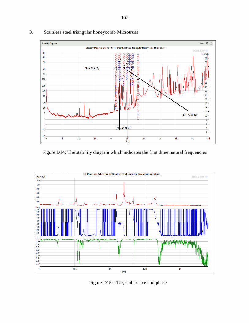
167
3. Stainless steel triangular honeycomb Microtruss
Figure D14: The stability diagram which indicates the first three natural frequencies
Figure D15: FRF, Coherence and phase

168
Figure D16: FRF results from RADIOSS
(Displacement contour)Mode1 Mode2 Mode3
Figure D17: 1st three mode shapes (displacement contour)
Figure D18: Maximum deflection for the 1st three modes
1.25E-05
2.14E-06 3.22E-06
0.00E+00
2.00E-06
4.00E-06
6.00E-06
8.00E-06
1.00E-05
1.20E-05
1.40E-05
Mode1 Mode2 Mode3
Max deflection( Stainless steel Microtruss)
Def
lect
ion(m
/N)
Mode #

169
Figure D19: Damping ratio for the 1st three modes
Figure D20: Compatibility between experiment and FEM results
0.047
0.15
0.083
0
0.02
0.04
0.06
0.08
0.1
0.12
0.14
0.16
Mode1 Mode2 Mode3
Damping ratio( Stainless steel Microtruss)
Dam
pin
g R
atio
(%)
Mode#
4275 4521
4769
4020 4172 4327
0
1000
2000
3000
4000
5000
6000
Mode1 Mode2 Mode3
Exp
FEM
Compatibilty results ( Stainless steel Microtruss)
Fre
quen
y(H
z)
Mode#

170
4. Aluminum nuts double in-line Micropillars
Figure D21: The stability diagram which indicates the first three natural frequencies
Figure D22: FRF, Coherence and phase

171
Figure D23: 1st three mode shapes (displacement contour)
Figure D24: Maximum deflection for the 1st three modes
Figure D25: Damping ratio for the 1st three modes
5.41E-04
4.36E-04
3.56E-04
0.00E+00
1.00E-04
2.00E-04
3.00E-04
4.00E-04
5.00E-04
6.00E-04
Mode1 Mode2 Mode3
Max deflection (Al nuts double in-line Micropillars)
Def
lect
ion(m
/N)
Mode #
0.58 0.64
0.72
0
0.1
0.2
0.3
0.4
0.5
0.6
0.7
0.8
Mode1 Mode2 Mode3
Damping ratio(Al nuts double in-line Micropillars)
Dam
pin
g R
atio
(%)
Mode #

172
REFERENCES
[1] Anon.,”Vibro-acoustics now key to automotive competition,” Noise and Vibration
Worldwide, June 2003, 13-15.
[2] Englehardt, K. J., and Toon, J., 2008, “Reducing Noise: Micro Honeycomb materials
enable a new physics of sound reduction,” Georgia Tech Research News, September 30,
2008.
[3] ’Boy, D.J., and Krylov, V. V., 2011, “Damping of flexural vibrations in circular plates
with tapered central holes,” Journal of sound and Vibration, 330, 2220-2236.
[4] J. C. Whitney, Inc., 2011, “Everything Automotive Catalogue”.
[5] Rao, S.S, “Mechanical Vibrations,” Prentice-Hall, London, 2003.
[6] Cerrato J. G et al. Automatic detection of buzz, squeak and rattle events, SAE Paper 2001-
01-1479; 2001
[7] Shin, S-H and Cheong, C.,”Experimental characterization of instrument panel buzz,
squeak and rattle (BSR) in a vehicle,” Applied Acoustics, (71) 2010 1162-1168.
[8] Karavarana F, Reiders B. Squeak and rattle – state of the art and beyond, SAE Paper 1999-
01-1728, SAE noise & vibration conference & exposition. Traverse City, Michigan; May
17–20, 1999.
[9] Gosavi, SS, Automotive buzz, squeak and rattle (bsr) detection and prevention, SAE
Paper, 2005, 26-56.
[10] Kreppold EM. A modern development process to bring silence into interior components.
SAE Paper 2007-01-1219, World Congress, Detroit, Michigan; April 16–19, 2007.
[11] Jay M, Gu Y. Excitation and measurement of bsr in vehicle seats. SAE Paper No. 2001-
01-1552; 2001.

173
[12] Poisson, S. D., “Memoir sur l’equibre et le movement des corp elastique,” M ‘em acad
Vol. 8, 1829.
[13] Kirchhoff, G., “ llber das Gleichgewicht und die Bewegung einer elastischer. Scheibe,”
Journal filr Math. (Crelle), Vol. 40, 1850.
[14] Rayleigh, L., (John W. Strutt) “The theory of sound,” Macmillan, London, 1894.
[15] Lamb, H. “Statics,” (Cambridge University Press, 1960; reprint of the third edition of
1928 of the textbook first published in 1912).
[16] Airey, J.R., “The vibrations of circular plates and their relation to Bessel functions,
Proceedings of the Physical Society of London Volume 23 ,p. 225, 1910.
[17] Timoshenko, S.P., “Vibration Problems in Engineering,” D. Van Nostrand Company, 1st
Ed. 1928, 2nd Ed. 1937, 3rd Ed. 1955 (with D. H. Young).
[18] Wood, A.B., “An experimental determination of the frequencies of free circular plates.
Authors: Wood, A. B.,” Proceedings of the Physical Society, Volume 47, Issue 5, pp.
794-799 (1935).
[19] Iguchi, S, 1937, “Allgemeine Lösung der Knickungsaufgabe für rechteckige Platten”.
Ingenieur-Archiv,vol.7,pp207-215
[20] Iguchi, S, 1953, “Die Eigenschwingungen und Klangfiguren der vierseiting freien
rechteckigen Platte durch Schubkrafte.Ingenieur-Archiv,vol.9,pp 1-12.
[21] Warburton, G.B., “The vibration of rectangular plates,” Proceedings of The Institution of
Mechanical Engineers. 168, 371-384 (1954).
[22] Lekhnitskii, S.G., Tsai, S.W., T. Cheron, T., “Anisotropic Plates,” (1947).
[23] Leissa, A.W., “Vibration of Plates,” NASA SP-160, U.S Gov’t Printing ffice. 10-13
(1969).
174
[24] Zelenev, Yu V., Electrova,L. M., Determination of the dynamic parameters of polymer
plates, Soviet Physical Acoustics 18 (1973) 339–341.
[25] Gorman, D.J. Free vibration analysis of cantilever plates by the method of superposition
Journal of Sound and Vibration, v 49, n 4, p 453-67, 22 Dec. 1976
[26] Gorman, D.J. ,”Free vibration analysis of rectangular plates with inelastic lateral support on
the diagonals,”Journal of the Acoustical Society of America, v 64, n 3, p 823-6, Sept.
1978.
[27] Gorman, D.J , “Highly accurate analytical solution for free vibration analysis of simply
supported right triangular plates,”..Journal of Sound and Vibration, v 89, n 1, p 107-118,
Jul 8 1983.
[28] Dickinson, S.M., “The bucking and frequency of flexural vibration of rectangular isotropic
and orthotropic plates using Rayleigh’s method,” J. Sound and Vibration. 61(1), 1-8
(1978).
[29] Dinis, L. M. S. and wen, D. R. J., “Elastic viscoplastic analysis of plates by the finite
element method.” Compui. Struct. 8, 207215 (1977). 20.
[30] Blevins, R.D., “Formulas for Natural Frequency and Mode Shape,” (1979).
[31] D.J. ’Connor, A finite element package for the analysis of sandwich construction,
Compos. Struct. 8 (1987), pp. 143–161.
[32] Ewins, D.J., “Modal Testing: Theory and Practice,” (1984).
[33] Deobald, L. R., Gibson. F., Determination of elastic constants of orthotropic plates by a
modal analysis/ Rayleigh–Ritz technique, Journal of Sound and Vibration 124 (1988)
269–283.

175
[34] Bardell, N.S.,”Free vibration analysis of a flat plate using the hierarchical finite element
method,” Journal of Sound and Vibration, v 151, n 2, p 263-89, 8 Dec. 1991.
[35] Lai, T.C, Lau, T.C.,”Determination of elastic constants of a generally orthotropic plate by
modal analysis, Modal analysis,” v 8, n 1, p 15-33, Jan 1993.
[36] L.J. Lee, Y.J. Fan., “Bending and vibration analysis of composite sandwich plates,”
Computers and Structures, v 60, n 1, p 103-12, 3 July 1995.
[37] Zhang, Q.J.; Sainsbury, M.G.,”Galerkin element method applied to the vibration of
rectangular damped sandwich plates, “Computers and Structures, v 74, n 6, p 717-730,
Febrary 1, 2000.
[38] Klosowski, K. Woźnica and D. Weichert “ Dynamics of elasto-viscoplastic plates and
shells “Archive of Applied Mechanics, Volume 65, Number 5 (1995), 326-345.
[39] Klosowski, P (1999). "Different types of constitutive equations in dynamic response of an
elasto-viscoplastic circular plate and cylindrical panel Arch". Civil engineering
(Johannesburg, South Africa)(1021-2000), 45(2), p.231.
[40] Hoshino, Hiroaki , Sakurai, Toshiaki; Takahashi, Kunihiro,”Vibration reduction in the
cabins of heavy-duty trucks using the theory of load transfer paths,” JSAE Review, v 24,
n 2, p 165-171, April 2003
[41] Sun, Liping,; Ai, Shangmao; Chen, Hailong,, “Vibro-acoustic statistical energy analysis of
a classic submarine structure, ”Harbin Gongcheng Daxue Xuebao/Journal of Harbin
Engineering University, v 27, p 507-512, December 2006.
[42] Pappada`, S.; Gren, P.; Tatar, K.; Gustafson, T.; Rametta, R.; Rossini, E.;Maffezzoli, A,
“.Mechanical and Vibration Characteristics of Laminated Composite Plates Embedding
176
Shape Memory Alloy Superelastic Wires,” Journal of Materials Engineering and
Performance, v 18, n 5-6, p 531-7, Aug. 2009
[43] Shin, S-H and Cheong, C.,”Experimental characterization of instrument panel buzz, squeak
and rattle (BSR) in a vehicle,” Applied Acoustics, (71) 2010 1162-1168.
[44] Cremer, L.L., “Theorie der schalldammung dummer wande bei schragen eingall,”
Acustica. 81 (1942).
[45] London, “Transmission of reverberant sound through double walls,” J. Acoust. Soc. Am.
22(2): 270 (1950).
[46] Zwikker, C., Kosten, C.W., “Sound Absorbing Materials,” Elsevier Publishing Company,
Inc. (1949).
[47] Vogel, T., “Sur les vibrations de certains systems elstiques damns un champ sonore,” Ph.
D. Thesis, Marseille (1947).
[48] Hickman, H.S.; Risty, D.E.; Stewart, E.S.,”Properties of sandwich-type structures as
acoustic windows” Acoustical Society of America -- Journal, v 29, n 7, p 858-864, July,
1957.
[49] Kurtze, G, “Bending wave propagation in multilayer plates,” Acoustical Society of
America -- Journal, v 31, n 9, p 1183-1201, Sept, 1959.
[50] Watters 1959 G. Kurtze and B.G. Watters, “New wall design for high transmission loss or
high damping,” Journal of the Acoustical Society of America, 31(6), 739-748 (1959).
[51] Maidanik, G., ”Response of ribbed panels to reverberant acoustic field,” J. Acoust. Soc.
Am. 34, 809-826 (1962).
[52] Ford, R.D.; Lord, P.; Walker, A.W., Sound transmission through sandwich constructions
Journal of Sound and Vibration, v 5, n 1, p 9-21, Jan, 1967.

177
[53] Sharp, B.H.S.; Beauchamp, J.W., “Transmission loss of multilayer structures, “Journal of
Sound and Vibration, v 9, n 3, p 383-392, May, 1969.
[54] Spronck, F, “Transparency to sound of thin plates,” Proceedings of the 7th international
congress on acoustics, p 301-4, 1971.
[55] Sewell, E. C. (1970). Transmission of Reverberant Sound through a Single-Leaf Partition
Surrounded by an Infinite Rigid Baffle. J. Sound Vib. Vol 12 , 21-32.
[56] Smolenski, C.P., Krokosky, E.M. Dilational-mode sound transmission in sandwich panels
Journal of the Acoustical Society of America, v 54, n 6, p 1449-57, 1973
[57] Dym, C.L., Lang, M.A.,”Transmission of sound through sandwich panels,” Journal of the
Acoustical Society of America, v 56, n 5, p 1523-32, Nov. 1974.
[58] Guyader, J.L., and Lesueur, C., ”Acoustic transmission through orthotropic multilayered
plates, Part II: Transmission Loss, ” J. Sound and Vibration. 58(1), 69-86 (1978).
[59] Woodcock, R., Nicolas, J., “A generalized model for predicting the sound transmission
properties of generally orthotropic plates with arbitrary boundary conditions,” J. Acoust.
Soc. Am. 97(2), (1995).
[60] Pates, Carl S., Mei, Chuh; Shirahatti, Uday.”Analysis of coupled structural-acoustic
problems using the boundary and finite element methods,” Collection of Technical
Papers - AIAA/ASME/ASCE/AHS/ASC Structures, Structural Dynamics and Materials
Conference, v 4, p 1835-1843, 1994.
[61] Fringuellino, M., Guglielmone, C., “Progressive impedance method for the classical
analysis of acoustic transmission loss in multilayered walls,” Applied Acoustics. 59
(2000).
178
[62] Lim, T.C ,”Automotive panel noise contribution modeling based on finite element and
measured structural-acoustic spectra,”. Applied Acoustics, v 60, n 4, p 505-19, Aug.
2000.
[63] Hills, E. , Mace, B.R.; Ferguson, N.S.,Acoustic response variability in automotive vehicles
Journal of Sound and Vibration, v 321, n 1-2, p 286-304, 20 March 2009.
[64] Wang binxing,; Zheng sifa; Zhoul lin; Liu shengqiang; Lian xiaomin; Li
keqiang,,”Acoustic modelling and analysis of vehicle interior noise based on numerical
calculation,” Proceedings of the 2010 International Conference on Intelligent
Computation Technology and Automation (ICICTA 2010), p 404-7, 2010.
[65] Dhaval Jain, “Modeling the characteristics of new-generation Ford vehicle panels for
efficient noise, vibration and harshness performance” .Master Thesis,Wayne State
University,2002.
[66] Lagrange, J. L., Volume XI: Mecanique Analytique (reprinted from second edition, 1811-
1815). Gauthier-Villars et fils, Paris:1888–89).
[67] Biot, M. A., Theory of propagation of elastic waves in a fluid-saturated porous solid. 1.
Low-frequency range", Journal of the acoustical society of America, vol. 28, March,
1956, pp. 168-178.
[68] Allard, Jean F., Depollier, Claude, Guignouard, Philippe, and Rebillard, Pascal, '"Effect of
A resonance of the frame on the surface impedance of glass wool of high density and
Stiffness", the Journal of the Acoustical Society of America, Vol. 89(3}, March, 1991,
pp. 999-1001.
[69] Wadley, H.N.G., (2002), ”Cellular metals manufacturing,” Advanced Engineering
Materials, 4(10), pp. 726 -733.

179
[70] Wadley,H.N.G., Fleck, N. A., Evans, A.G., (2003),”Fabrication and structural performance
of periodic cellular metal sandwich structures,” Composites Science and Technology 63,
2331–2343.
[71] Bruel and Kjaer,”PULSE multi-analyzer system type 3560, installation hardeware”2009.
[72] Bruel and Kjaer., “Two Microphone Impedance Tube Theoretical Manual,” (1992).
[73] Dossing, ., Bruel and Kjaer., “Structural Testing (Part I, II) User Manual,” (1988).
[74] Bruel and Kjaer,” Hammer demo guide, modal analysis using PULSE”, 2009.
[75] Bruel and Kjaer,”Pulse Reflex modal analysis, version 16.1” 2011.
[76] Peter Wides,”Introduction to finite element analysis”, Virginia Tech, 1997.
[77] Abaqus Analysis User's Manual, Dassault Systems, 2009.
[78] Altair Engineering Inc. “RADI SS theory manual “,version 10,2009.
[79] Yang, “Stress, Strain and Structural Dynamics”, Book, 2005, Elsevier.
[80] Huoy-Shyi Tsay, Fung-Huei Yeh,” The influence of circumferential edge constraint on the
acoustical properties of open-cell polyurethane foam samples”, Journal of Acoustical
society of America,pp 2804-2814,2006.
[81] J.Pfretzschner,F.Simon,R.M Rodriguez,and C. de la Colina,” Simplified calculus to
estimate the acoustical absorption of non-planar materials”, Institute de Acustica
(CSIC),1999.
[82] J. Pfretzschner, R. Mª. Rodríguez,” Acoustical absorption and critical thickness” Instituto
de Acústica-CSIC. C/ Serrano, 144. 28006 Madrid-Spain,2001.
[83] Everst. F.A,”The master handbook of acoustics”,2nd edition, tab books,1989.
[84] Jaesuk Lee, “ Low velocity impact and sound absorption of composite sandwiches”
,Dissertation, Wayne State University, 1999.

180
ABSTRACT
INVESTIGATION AND IMPROVEMENT OF NOISE, VIBRATION AND HARSHNESS
(NVH) PROPERTIES OF AUTOMOTIVE PANELS
by
MOHAMMAD AL-ZUBI
August 2012
Advisor: Dr. Emmanuel Ayorinde
Major: Mechanical Engineering
Degree: Doctor of Philosophy
The reduction of noise and vibration in and across several components and modules of the
automotive, such as the panels, doors, engine covers, seats, and others, is of primary importance.
The NVH performance may be a crucial factor in the purchase decisions of numerous buyers.
This work investigates through experimental, analytical and computational methods, six groups
of sample materials - fabric, foam, honeycomb, monolithic and sandwich, periodic cellular
material structures (PCMS), and generally periodic materials, to assess their suitability for
maximum containment of noise and vibration. Various architectural forms have also been
considered. State-of-the art instrumentation and adequate analytical and computational methods
have been utilized. Five major novel accomplishments have been logged in the work. Vibro-
acoustic responses of PCMS materials and newly-constructed generally periodic materials are
explored, and some computer procedures are generated. The results give some suggestions for
design directions to follow in order to achieve better performances.

181
AUTOBIOGRAAPHICAL STATEMENT
MOHAMMAD AL- ZUBI
Mohammad Ahmed AL Zubi was born on October 18, 1972 in Jordan. He received his bachelor
degree in Mechanical Engineering from the Mu’tah University in Jordan, 1994. Upon
graduation, he started working as a maintenance engineer in the Royal Jordanian Air Force until
2008; during his service he got his Master degree in Industrial Automation Engineering in 2006.
Mohammad got a scholarship from his government in 2009, then he joined Wayne State
University as a PhD student in September 2009, he was a graduate teaching assistance from 2010
to 2012. Mohammad has published several papers in ASME conferences; also he submitted two
Journal papers before his defense. Upon receiving his doctoral degree Mohammad will go back
to his country Jordan to continue his academic life as a professor at Tafila Technical University.
He hopes to continue his research in the areas of automotive NVH.