INVESTIGATING THE ROLE OF DEM RESOLUTION AND ACCURACY ON

FLOOD INUNDATION MAPPING

A Thesis

Submitted to the Faculty

of

Purdue University

by

Siddharth Saksena

In Partial Fulfillment of the

Requirements for the Degree

of

Master of Science in Civil Engineering

May 2014

Purdue University

West Lafayette, Indiana

ii

For my parents

iii

ACKNOWLEDGEMENTS

I would like to thank my advisor Prof. Venkatesh Merwade for his constant support, time

and guidance. I would also like to thank Prof. Dennis Lyn and Prof. Keith Cherkauer for

serving on my committee.

The data for this study was provided by USGS Indiana Water Data Center, North Carolina

Floodplain Mapping Program (NCFMP) and Fort Bend County, Texas. This study would

not have been possible without this data.

Finally I would like to thank my colleague and friend Adnan Rajib for his feedback and

my roommates Vaidehi Paranjape, Mohneet Ahuja and Anuj Choudhari for their support.

iv

TABLE OF CONTENTS

Page

TABLE OF CONTENTS ................................................................................................... iv LIST OF TABLES ............................................................................................................ vii LIST OF ABBREVIATIONS ........................................................................................... xii ABSTRACT…………………………………………………………………………… . xiii CHAPTER 1.  INTRODUCTION ................................................................................. 1 

1.1  Background and Study Objective ..............................................................1 

1.2  Approach ....................................................................................................4 

1.3  Thesis Organization.. .................................................................................5 

CHAPTER 2.  LITERATURE REVIEW ...................................................................... 6 2.1  Introduction ................................................................................................6 

2.2  Effect of Topography and DEM Resolution on Hydraulic Modeling........6 

2.3  Effect of DEM Accuracy and Error on Hydraulic Modeling ...................13 

2.3.1  Case Studies on Spatial Distribution of DEM Errors........................15 

2.3.2  Errors due to Interpolation and Sampling Technique .......................17 

2.4  Summary ..................................................................................................19 

CHAPTER 3.  STUDY AREA AND DATA .............................................................. 21 3.1  Introduction ..............................................................................................21 

3.2  Description of River Reaches ..................................................................21 

3.2.1  Strouds Creek ....................................................................................21 

3.2.2  Tippecanoe River ..............................................................................22 

3.2.3  St. Joseph River .................................................................................24 

3.2.4  East Fork White River .......................................................................25 

3.2.5  Clear Creek .......................................................................................26 

3.2.6  Brazos River ......................................................................................27 

3.3  Description of Flow Data .........................................................................28 

3.4  Description of LiDAR Data .....................................................................29

v

Page

CHAPTER 4.  METHODOLOGY .............................................................................. 30 4.1  Introduction ..............................................................................................30 

4.2  Description of 1-D HEC-RAS .................................................................30 

4.3  Terrain Pre-processing using ArcGIS ......................................................32 

4.4  Description of Topographic Datasets .......................................................36 

4.4.1  Effect of DEM Resolution on Hydraulic Outputs .............................36 

4.4.2  Effect of DEM Error on Hydraulic Outputs ......................................37 

4.5  Hydraulic Modeling using 1-D HEC-RAS ..............................................39 

4.6  Creation of Flood Maps ...........................................................................40 

CHAPTER 5.  RESULTS ............................................................................................ 41 5.1  Introduction ..............................................................................................41 

5.2  Effect of DEM Resolution on Hydraulic Outputs ....................................41 

5.2.1  Study Areas with small size and urban land use ...............................42 

5.2.2  Study Areas with large size and agricultural land use ......................53 

5.3  Effect of DEM Error on Hydraulic Outputs .............................................61 

5.3.1  RMSE of Elevations versus Grid Size ..............................................61 

5.3.2  Effect of Error Introduction in DEMs on Hydraulic Outputs ...........64 

5.4  Summary of Results .................................................................................69 

CHAPTER 6.  DISCUSSIONS ................................................................................... 71 6.1  Introduction ..............................................................................................71 

6.2  Development of New Analysis Approach ...............................................72 

6.3  Testing and Application of the New Approach .......................................73 

6.3.1  Prediction of Water Surface Elevations ............................................75 

6.3.2  Prediction of Flood Maps ..................................................................84 

6.4  Validation and Estimation for Different Topographic Datasets ..............87 

6.4.1  USGS NED 30 m Resolution DEMs ................................................88 

6.4.2  SRTM 90 m Resolution DEMs .........................................................95 

6.5  Comparison of Resampling Techniques ................................................101 

6.6  Incorporation of River Bathymetry ........................................................103 

CHAPTER 7.  SUMMARY AND CONCLUSIONS ................................................ 107 7.1  Effect of DEM Resolution on Hydraulic Outputs ..................................107

vi

Page

7.2  Effect of DEM Error on Hydraulic Outputs ...........................................108 

7.3  Development of a New Approach to Reduce the Impact of Errors .......109 

7.4  Future Work and Recommendations ......................................................111 

LIST OF REFERENCES ................................................................................................ 114 

vii

LIST OF TABLES

Table Page

3.1 Description of flow data……………………………...………………………………29

5.1 Hydraulic outputs for Strouds Creek………………………………………………….43

5.2 Hydraulic outputs for Tippecanoe River……………………………………………...44

5.3 Hydraulic outputs for St. Joseph River……………………………………………….45

5.4 Hydraulic outputs for East Fork White River…………………………………………54

5.5 Hydraulic outputs for Brazos River…………………………………………………..55

5.6 RMSE versus grid size………………………………………………………………..61

5.7 Hydraulic outputs for DEMs with error (Strouds Creek)……………………………..64

6.1 Hydraulic outputs for Clear Creek……………………………………………………74

6.2 Comparison between observed and predicted results for Clear Creek………………..75

6.3 Prediction of WS El. for LiDAR using coarser resolution data……………………….77

6.4 RMSE between observed and predicted WS El. for six study areas…………………..80

6.5 Comparisons of flood maps for Tippecanoe River and Clear Creek………………….86

6.6 RMSE of predicted and USGS WS El………………………………………………...93

6.7 Comparison of flood maps for East Fork White River and Strouds Creek……………93

6.8 RMSE of predicted and SRTM WS El………………………………………………..98

6.9 Comparison of flood maps for Brazos River and Strouds Creek……………………...98

viii

Table Page

6.10 Average Elevation and RMSE for St. Joseph River and Tippecanoe River………...104

6.11 Comparison of flood maps for St. Joseph River and Tippecanoe River……………105

ix

LIST OF FIGURES

Figure Page 3.1 Strouds Creek study area……………………………………………………………..22

3.2 Tippecanoe River study area……………………………………………………….....23

3.3 St. Joseph River Study Area…………………………………………………………..24

3.4 East Fork White River Study Area……………………………………………………25

3.5 Clear Creek Study Area………………………………………………………………26

3.6 Brazos River Study Area……………………………………………………………..28

3.7 Terrain Pre-Processing for Strouds Creek and Tippecanoe River…………………….33

3.8 Terrain Pre-processing for St. Joseph River and East Fork White River……………...34

3.9 Terrain Pre-processing for Brazos River and Clear Creek……………………………35

5.1 Cross-section station 6152.8 across Strouds Creek for

(a) LiDAR; (b) resampled 100 m DEM………………………………………………46

5.2 Cross-section station 269.5 across Tippecanoe River for

(a) LiDAR; (b) resampled 100 m DEM………………………………………………46

5.3 Cross-section station 4736 across St. Joseph River for

(a) LiDAR; and (b) re-sampled 100 m DEM…………………………………………47

5.4 Grid size versus (a) avg. WS El.; and (b) inundated area for Strouds Creek…………..48

5.5 Grid size versus (a) avg. WS El.; and (b) inundated area for Tippecanoe River………48

x

Figure Page

5.6 Grid size versus (a) avg. WS El.; and (b) inundated area for St. Joseph River………...49

5.7 Flood maps generated from different resolution DEMs for Strouds Creek…………..50

5.8 Flood maps generated from different resolution DEMs for Tippecanoe River……….51

5.9 Flood maps generated from different resolution DEMs for St. Joseph River…………52

5.10 Cross-section Station 19206.5 across East Fork White River for

(a) LiDAR; (b) resampled 100m DEM……………………………….……………..56

5.11 Cross-section station 33160.7 across Brazos River for

(a) LiDAR; and (b) resampled 100 m DEM…………………………………………56

5.12 Grid size versus (a) avg. WS El.; and (b) inundated area for White River…………...57

5.13 Grid size versus (a) avg. WS El.; and (b) inundated area for Brazos River…………..58

5.14 Flood maps generated from different resolution DEMs for White River……………59

5.15 Flood maps generated from different resolution DEMs for Brazos River…………...60

5.16 RMSE versus grid size for (a) St. Joseph River; (b) Tippecanoe River;

and (c) Strouds Creek……………………………………………………………….63

5.17 Grid size versus (a) avg. WS El.; and (b) inundated area for Strouds Creek…………66

5.18 Cross-section station 6512.8 for (a) LiDAR; (b) 12 m DEM with error;

(c) 30 m DEM with error; and (d) 80 m DEM with error…………………………….67

5.19 Flood maps generated from (a) LiDAR; (b) 12 DEM with error;

(c) 30 m DEM with error; and (d) 80 m DEM with error…………………………….68

xi

Figure Page

6.1 Grid size versus (a) avg. WS El.; and (b) inundated area………………………….…74

6.2 Predicted WS El. versus original LiDAR (base) WS El. along the line Y=X…………78

6.3 Water surface profiles for (a) Brazos River; (b) Clear Creek;

(c) East Fork White River…………………………………………………………….81

6.4 Predicted versus LiDAR (base) WS El. for Strouds Creek along Y=X………………83

6.5 Water surface profile comparison for (a) predicted (new approach);

(b) LiDAR (base); and (c) 30 m resampled DEM with error………………………….84

6.6 WS El. versus grid size for USGS and LiDAR DEMs………………………………..89

6.7 LiDAR (base) versus predicted WS El. for (a) East Fork White River and

(b) Strouds Creek..........................................................................................................92

6.8 Inundation extents for East Fork White River and Strouds Creek…………………….94

6.9 WS El. of SRTM DEMs versus grid size for

(a) Strouds Creek and (b) Brazos River……………………………………………....96

6.10 LiDAR (base) versus predicted WS El. for

(a) Strouds Creek and (b) Brazos River……………………………………………..97

6.11 Inundation extents for Brazos River and Strouds Creek……………………………..99

6.12 Avg. WS El. versus grid size for (a) Brazos River and (b) East Fork White River….102

6.13 Avg. WS El. versus grid size for Bathymetry LiDAR for St. Joseph River………...105

6.14 Inundation Extents for (a) St. Joseph River and (b) Tippecanoe River……………..106

xii

LIST OF ABBREVIATIONS

1D One-dimensional

2D Two-dimensional

DEM Digital Elevation Model

DTM Digital Terrain Model

FEMA Federal Emergency Management Agency

GIS Geographic Information System

HEC-RAS Hydrologic Engineering Center River Analysis System

IfSAR Interferometric Synthetic Aperture Radar

LiDAR Light Detection and Ranging

NED National Elevation Dataset

RMSE Root Mean Squared Error

SRTM Shuttle Radar Topography Mission

USGS United States Geological Survey

WS El. Water Surface Elevations

xiii

ABSTRACT

Saksena, Siddharth. M.S.C.E., Purdue University, May 2014. Investigating the Role of DEM Resolution and Accuracy on Flood Inundation Mapping. Major Professor: Venkatesh Merwade. Topography plays an important role in determining the accuracy of flood inundation maps.

A lot of the current flood inundation maps are created using topographic information

derived from Light Detection and Ranging (LiDAR) data. Although LiDAR data is very

accurate, it is expensive, computationally time consuming and not available in several areas

across the United States and around the world. As a result, coarser resolution DEMs which

are easily available but less accurate are used for flood modeling. It is essential to

understand the properties of LiDAR data to create methods to modify coarser resolution

DEMs and increase their accuracy. These properties can be used to understand how

elevation errors propagate within a DEM and reduce the impact of errors in coarser

resolution datasets.

The first objective of this study is to quantify the errors arising from DEM properties such

as resolution and accuracy on flood inundation maps. The results from these six study areas

show that water surface elevations and flood inundation area have a linear relationship with

the DEM resolution and accuracy.

xiv

The second objective of this study is to use the linear relationship between hydraulic

outputs and the DEM resolution or accuracy to create an approach for developing accurate

flood inundation maps using less accurate DEMs by modeling the spatial distribution of

DEM errors. Application of this new approach on USGS NED 30 m resolution DEMs and

SRTM 90 m resolution DEMs shows significant increase in the accuracy of water surface

elevations and improvement in predicted flood extents created from coarser resolution

DEM when compared to results from high resolution accurate DEMs.

A check on the applicability of this approach for different interpolation methods and river

channel conditions is also made in this study. The new approach thus provides promising

results in obtaining more accurate flood maps from less accurate topographic data.

1

CHAPTER 1. INTRODUCTION

1.1 Background and Study Objective

Floods are one of the major natural disasters in the United States accounting to losses worth

$8.17 Billion (National Weather Service) over the past 30 years. The majority of flood

inundation maps in the US are prepared by the Federal Emergency Management Agency

(FEMA) that are useful in identifying flood risk areas. Flood Inundation Mapping involves

analysis of river flow data, hydrologic/hydraulic modeling and topographic surveys. Water

surface elevations (WS El.) and flood extents are the two major components of flood

inundation mapping. Hydraulic modeling is primarily carried out using Hydrologic

Engineering Center-River Analysis System (HEC-RAS) which has been designed and

developed by United States Army Corps of Engineers (USACE 2006).

Topography plays a major role in determining the accuracy of hydraulic modeling and

flood inundation mapping (Brandt, 2005; Cook & Merwade, 2009). Digital Elevation

Model (DEM) is a raster dataset containing information about the topography of a region

and is used as a prerequisite to hydraulic modeling.

2

For hydraulic modeling purposes, DEMs are used to determine the active channel cross-

sectional elevations, water surface elevations and flood extents. Resolution and accuracy

are the two main properties of a DEM that affect hydraulic and hydrologic modeling results

(Vaze et al., 2010).

The spatial resolution of a DEM refers to the area covered on the ground surface by a single

cell which suggests that a higher resolution DEM has more number of cells per unit area

and thus represents the topography more accurately as compared to a coarser resolution

DEM (ESRI, 2014a). Resolutions of DEMs can affect the parameters and attributes derived

from them and influence models associated with them (Gallant & Hutchinson, 1997; Haile

& Rientjes, 2005; Omer et al., 2003). The vertical accuracy of a DEM is the probability

distribution of digital elevation values measured with respect to the true value. It is

measured by the amount of linear error in elevation (ESRI, 2014b). The accuracy of a DEM

directly influences the hydraulic modeling results (Darnell et al., 2008; Fisher & Tate,

2006). Thus, DEM resolution and accuracy have a significant impact on water surface

elevations and flood extents.

DEMs obtained from LiDAR data have a high resolution and accuracy and are used

extensively for hydraulic modeling purposes (Cook & Merwade, 2009; Rayburg et al.,

2009). The water surface elevations and flood maps obtained on using LiDAR data are

more accurate than the other widely used DEMs present in the world (Charlton et al., 2003;

Schumann et al., 2008).

3

But there are several areas within the United States and around the world where LiDAR

data are still unavailable. The use of LiDAR data is not feasible for some locations due to

time constraints and cost of acquisition even though they are the most accurate topographic

data source (Sanders, 2007).

For the areas where LiDAR data are unavailable, it is desirable to study how the hydraulic

modeling and flood inundation results can be improved using the existing coarser

resolution and low accuracy topographic datasets. This thesis focuses on the impact of two

key attributes of topographic data: (1) resolution; and (2) accuracy on hydraulic modeling

and flood inundation mapping using LiDAR data. The study of these attributes seeks to

understand their relationships with hydraulic outputs so that these relationships can be

applied to coarser resolution and low accuracy datasets to obtain better hydraulic modeling

and flood inundation mapping results. Thus, the two main research objectives of this study

based on DEM resolution and accuracy are:

(1) Studying the impact of DEM resolution or grid size on water surface elevations and

flood inundation extents

(2) Evaluating the impact of DEM errors on water surface elevations and flood

inundation extents

In order to accomplish these research objectives, the method of DEM resampling and error

analysis is used. The results of hydraulic analysis can vary significantly for different study

areas, land use types and river reach lengths.

4

Therefore, six study areas with different topography, land use, reach lengths and flow

conditions are selected for this study. The thesis also aims to find a threshold for DEM grid

sizes and errors above which the hydraulic analysis results are unacceptable using these

study areas.

1.2 Approach

The objectives of this thesis are accomplished by analyzing the results obtained from flood

inundation mapping for six reaches of different reach lengths and land use types. Flood

mapping for these reaches is carried out by 1D HEC-RAS modeling using LiDAR

topographic datasets. 100-year flow values are calculated using Log-Pearson Type III

distributions for peak annual observed flows provided by United States Geological Survey

(USGS).

The first task to attain the objectives of this study involves resampling the LiDAR datasets

into DEMs of different resolutions and using these datasets for hydraulic modeling. The

results for the second objective are obtained by introducing elevation errors of different

magnitudes into the LiDAR DEMs for these reaches. The results are compared with flood

maps obtained from original LiDAR datasets as base maps.

The assumption with this approach is that the original LiDAR datasets are the most

accurate topographic datasets even though the predicted flood maps are not completely

accurate when compared to observed flood depths and extents.

5

However, the high resolution LiDAR datasets offer superior results in estimating the flood

inundation area and river networks when the cell sizes are less than 10 m (Li & Wong,

2010; Rayburg et al., 2009).

1.3 Thesis Organization

This thesis is organized in 7 chapters. Chapter 2 presents a review of previous case studies

on the effect of topography and DEM resolution on hydraulic modeling. This chapter also

presents previous studies on DEM error analysis. Chapter 3 presents a description of study

areas and the data used for this study. Chapter 4 presents the methodology used for

producing results and analysis techniques used for different variables. The methodology

used to digitize the different areas is explained first followed by a description of creating

different topographic datasets which are used for flood mapping. Chapter 5 present the

results obtained from this study. The results are divided into two sections discussing the

impact of DEM resolution and DEM error on hydraulic outputs. Chapter 6 discusses the

application of the obtained results to reduce the impact of DEM resolution and DEM errors.

This section describes a new approach to improve the predicted water surface elevations

and flood inundation areas obtained from coarser resolution datasets. Chapter 7 presents

the summary and conclusions for this study.

6

CHAPTER 2. LITERATURE REVIEW

2.1 Introduction

The effect of two attributes on water surface elevations and flood extents are analyzed in

this thesis; changing the resolution of topographic data, and varying the magnitude of

vertical error in the elevations to determine the impact of DEM accuracy. DEMs with larger

grid sizes have less detailed information as they have one elevation value for a larger area.

DEMs with high resolution or smaller grid sizes represent elevations of smaller areas and

can better represent the smaller topographic details. Case studies on the effect of resolution

of topographic data are discussed in Section 2.2. The effect of DEM errors and previous

case studies discussing the significance of these errors on hydraulic modeling are presented

in Section 2.3.

2.2 Effect of Topography and DEM Resolution on Hydraulic Modeling

With the advent of GIS based techniques to obtain channel cross-sections, topographic

datasets have become essential in flood mapping. The cross-section elevations obtained

from topographic datasets are used for hydraulic modeling in HEC-RAS to produce water

surface elevations. Flood extent is obtained by subtracting the topography from the

interpolated water surface obtained through hydraulic modeling (Tate et al., 2002).

7

This section reviews the past studies that have established the importance of topography

and DEM resolution.

In order to understand the importance of topography and DEM resolution, it is essential to

look at the source of the DEMs that are used for hydraulic modeling. The National

Elevation Dataset (NED) provided by the United States Geological Survey (USGS) are the

most widely used DEMs in the United States. The NED 30 m resolution DEMs are often

obtained from cartography or photogrammetry and are of low quality due to the existence

of artifacts (Gesch et al., 2002). Even though these artifacts are filtered to some extent,

these are coarser resolution DEMs with lower accuracy.

The DEMs of higher resolution and accuracy are obtained through the LiDAR (Laser

Interferometry Detection and Ranging) remote sensing technology. The quality of LiDAR

DEMs depends upon the sampling and filtering methods (Chu et al., 2014). LiDAR

technology serves as an accurate survey tool for obtaining highly accurate topographic

datasets (Charlton et al., 2003). However, many places in the United States and around the

world do not have the resources to obtain LiDAR data, and therefore, DEMs of coarser

resolutions like USGS DEMs are used for hydraulic modeling where LiDAR DEMs are

unavailable.

Hydraulic modeling and flood mapping using LiDAR data produces more accurate results

when compared to other available topographic datasets. This was suggested by comparing

the performances of four on-line DEMs (LiDAR, NED, SRTM and IfSAR) on flood

8

inundation modeling and the study was carried out for Santa Clara River near Castaic

Junction in southern California and Buffalo Bayou near downtown Houston in Texas

(Sanders, 2007). The results of this study clearly show that LiDAR DEMs represent best

the terrain for flood mapping since they have the highest horizontal resolution and vertical

accuracy. IfSAR DEMs require further processing to incorporate the vegetation, bridges

and buildings before use in flood mapping. SRTM DEMs generate the least accurate results

due to existence of radar speckles but their global availability is significant in flood

mapping. NED DEMs are more accurate in comparison to SRTM and IfSAR generated

DEMs but often over-predict the flood inundations. This study however, did not compare

the performance of LiDAR with surveyed data.

In order to evaluate the performance of LiDAR data when compared to surveyed data,

Casas et al. (2006) carried out a study of accuracy of topographic dataset sources in

hydraulic modeling for Ter River near Sant Juliá de Ramis, 5 km downstream of Girona in

NE Spain which consisted of Digital Terrain Models (DTMs) from three different sources:

high resolution LiDAR, global positioning system (GPS) survey and vectorial cartography.

Hydraulic modeling was carried out using HEC-RAS and water surface elevations and

delineated flooded area were analyzed. The contour-based DTM performed with the least

accuracy with a variation of 50% in the flood inundation determination. The LiDAR dataset

for this study area performed with the highest accuracy with less than 1% variation and

GPS-based DTMs produced maps of less than 8% variation from the observed data. The

results also showed that the DTM quality and its resolution determine the accuracy of flood

predictions.

9

The hydraulic modeling for the two studies described above was carried out using HEC-

RAS. These studies showed that the performance of LiDAR DEMs was superior to the

other available DEMs (USGS, IfSAR and SRTM) as well as DEMs derived from different

sources (GPS survey, photogrammetry and cartography).

In order to evaluate the performance of topographic datasets using a different hydraulic

modeling technique, a study based on remote sensing technology by Schumann et al. (2007)

demonstrated the use of synthetic aperture radar (SAR) images of moderate resolution to

determine the water-line during a flood event. This approach used high resolution LiDAR

DEMs to extract elevation values for cross-sections across River Alzette situated

downstream of Luxemburg city in England. A Regression and Elevation-based Flood

Information Extraction (REFIX) model was developed which used remotely sensed flood

extents observed during a flood event and linear regression to calculate flood depths. The

REFIX model compared the water stages obtained from three different topographic dataset

sources. The results showed that LiDAR datasets had the least RMSE (0.35 m) when

compared to contour DEM (0.7 m) and SRTM (1.07 m). This study also indicated that

flood mapping with coarser DEMs for a small area presented a lot of uncertainties and high

resolution data was required to measure the elevations accurately (Schumann et al., 2008).

From the studies described above, it can be concluded that LiDAR data is the most accurate

topographic dataset available for hydraulic modeling irrespective of the modeling approach.

It is however essential to develop techniques to increase the accuracy of the other coarser

DEMs in order to increase their applicability in hydraulic modeling.

10

One of the most important properties of a DEM affecting hydraulic modeling results is its

resolution. In order to increase the prediction accuracy of DEMs, it is essential to

understand the importance of DEM resolution on flood mapping. Many studies were

carried out analyzing the effect of changing DEM resolution on hydraulic modeling which

concluded that DEM resolution played a significant role in predicting hydraulic outputs.

One of the first studies by Werner (2001) in analyzing the impact of grid size on accuracy

of predicted flood areas showed that hydraulic controls such as embankments have a

significant effect on the accuracy of flood extents. Local elevations around the hydraulic

controls averaged out on using a coarser resolution DEM while the use of higher resolution

DEMs increased the computational time significantly.

This study suggested that one significant disadvantage of coarser resolutions was the

inaccuracy in determining correct elevations for bridges, embankments and levees. While

this problem could be corrected by using field surveyed elevations and locations for

hydraulic controls, the overall effect of decreasing DEM resolutions on predicted flood

extents is still significant and further studies were carried out to evaluate this effect.

Haile et al. (2005) studied the effects of changing DEM resolution for an urban city

Tegucigalpa in Honduras. In this study, a DEM of grid size 1.5 meters was generated using

LiDAR data and resampled to DEMs with decreasing resolutions up to 15 meters. 2-D

SOBEK flood model was used to evaluate flood inundation extents.

11

This study concluded that the DEM with the largest grid size predicted maximum inundated

area and downstream boundary condition had no significant effect on the flood area. The

averaging of small-scale topographic features and arbitrary delineation of flow direction

for larger grid sizes were identified as the possible causes for variation in flood area.

This study highlighted the significance of DEM resolution for an urban study area using a

2-D hydraulic model and suggested the reasons for the lower accuracy of coarser resolution

DEMs. Since 2-D hydraulic modeling is complex and 1-D HEC-RAS modeling is used

more frequently in the world, it was desirable to determine the impact of DEM resolution

for 1-D hydraulic models.

Such a study at Eskilstuna River in Sweden was carried out by Brandt (2005) to show the

effect of different DEM resolutions on inundation maps using 1-D HEC-RAS. The results

showed that higher resolution DEMs produced better and more precise flood maps.

However, all the cross sections used in the hydraulic model were determined from high

resolution DEMs. Resampled DEMs were used only to calculate the inundated areas after

the water surface elevations were generated from HEC-RAS. This study also concluded

that high resolution data produced much better results for small and narrow rivers. For

bigger and wider rivers (about 20 km long and 300 m wide), coarser resolution data also

generated fairly close results. The use of 1-D hydraulic modeling was justified for rivers

with a significantly well-defined valley as there was not much difference in the output of

1-D and 2-D models for such rivers.

12

For the United States, the effect of DEM resolution was analyzed for Strouds Creek in

North Carolina and Brazos River in Texas by Cook et al. (2009). The results clearly showed

that for a steady state flow assumption, the predicted flood inundation extent decreased by

6% for Strouds Creek on using higher resolution topographic data. The predicted flood area

increased by 4% for Strouds Creek and Brazos River on doubling the number of cross

sections which suggested that the cross sections should be placed at strategic locations.

To understand the causes for the over-prediction of flood extents by coarser resolution

DEMs, a study on the effect of cell resolution on depressions was carried out by

Zandbergen (2006) for a 6 m LiDAR DEM in Middle Creek, North Carolina. The study

suggested that the occurrence of depressions in digital elevation models could also affect

the hydraulic modeling results. Although there were techniques to remove these

depressions from the DEM such as depression filling and breaching, they were meant for

depressions caused artificially. For a flat terrain, removal of a real depression can have a

significant impact on hydraulic predictions. Higher resolution DEMs derived from LiDAR

data give an accurate estimate of real and artificial depressions and thus contain a large

number of depressions. The results produced in this study clearly established that DEM

resolution had a significant impact on the number of depressions. Depressions decreased

with decreasing resolution following an inverse power relationship. The study also

concluded that coarser DEMs had a lower number but a higher total volume of depressions

while DEMs between 30 m and 61 m had minimum area and volume of depressions. A

scale-dependence of the number of depressions was suggested for high resolution DEMs.

13

All the studies suggested that coarser resolution DEMs over-predicted the flood extents

and resulted in significant loss of accuracy. Some of these studies also tried to analyze the

causes of the over-prediction. It was established that coarser DEMs had a significant

smoothing effect on the cross-sections. But these studies did not try to establish a

relationship between DEM resolution and hydraulic outputs. If a mathematical relationship

between the predicted results for different grid sizes of DEMs is established, the accuracy

of prediction for coarser DEMs can be increased significantly, which is one of the

objectives of the current study.

2.3 Effect of DEM Accuracy and Error on Hydraulic Modeling

In order to investigate the role of errors in DEMs, it is essential to understand the sources

of errors. There are three possible sources of errors which can occur in a DEM: (1) errors

due to spatial sampling; (2) measurement errors due to positional inaccuracy; and (3)

random errors including interpolation errors and computer generated numerical errors

(Burrough, 1986). A lot of methods have been adopted to remove these errors from the

gridded DEMs but it is difficult to remove them completely.

The focus of the current study is to determine the impact of DEM errors on hydraulic

modeling and use this knowledge to develop techniques for reducing this impact for coarser

resolution DEMs. A study by Smith et al. (2004) on the accuracy analysis of gridded Digital

Surface Models (DSMs) created from LiDAR data highlighted the importance of errors in

vertical accuracy of data. The results indicated a need to model not only the global errors,

but also individual errors based on location and magnitude.

14

The analysis suggested that the existence of errors could affect any subsequent analysis

using DSMs. After establishing that DEM errors can affect the subsequent analysis results

significantly, it is essential to compare and quantify the magnitude of error occurring in

different DEMs available for hydraulic modeling.

Gonga-Saholiariliva et al. (2011) conducted a comparative analysis of DEMs derived from

six different sources (airborne, radar, optical and composite) for Wasatch Mountain Front

in Utah. These DEMs included a LiDAR (2 m), CODEM (5 m), NED 10 (10 m), ASTER

DEM (15 m), GDEM (30 m) and SRTM (90 m). The results show that LiDAR DEMs have

the least errors followed by NED 10 which is generated from composite data sources.

CODEM and ASTER DEM show high magnitude of errors even after having high ground

resolutions. This study highlighted the importance of source-study before processing and

delivering the final product.

Similarly, Hodgson et al. (2003) studied the differences occurring in vertical accuracy

estimates of LiDAR, IfSAR, NED 10 m and NED 30 m for Swift and Red Bud Creeks in

North Carolina. All the DEMs over-predicted the average elevations regardless of land use

types with LiDAR data being the most accurate with an RMSE of 93 cm followed by NED

10 m (163 cm), NED 30 m (743 cm) and IfSAR (1067 cm).

The results clearly indicate that LiDAR data is currently the most accurate data containing

the least amount of errors. This is true for DEMs derived from different sources as well as

different resolutions.

15

However, the accuracy of the other DEMs in hydraulic modeling can be improved if these

errors can be modeled correctly and removed from the DEMs. This requires studies of

spatial distribution and source of errors for different DEMs which are presented in Section

2.3.1 and Section 2.3.2.

2.3.1 Case Studies on Spatial Distribution of DEM Errors

A significant percentage of DEM errors are random in nature. However, studies have been

carried out to model these errors and obtain a spatial distribution. Aguilar et al. (2006) tried

to model DEM errors by conducting a detailed study using linear interpolation of scattered

sample data in Almería, south-eastern Spain. A model was developed to determine the error

when randomly scattered data points were linearly interpolated into gridded sample points.

The model consisted of an empirical error caused due to sampling (information loss) and a

theoretical error based on error propagation theory. However, this was a theoretical

scenario and linear interpolation is not used frequently to create DEMs.

Therefore, Aguilar et al. (2010) carried out a follow-up study for 29 datasets in Almería

using Inverse Distance Weighing (IDW) instead of linear interpolation and developed a

methodology to model vertical errors occurring in LiDAR datasets. This model expressed

the error as a sum of three components: (1) error in LiDAR data capture from ground points;

(2) gridding error; (3) filtering of non-terrain objects such as vegetation and buildings. The

results showed a very good fit between observed and predicted errors (R2=0.9856;

p<0.001). The model was also validated for two LiDAR datasets including Ordnance

Survey data for Bristol, UK and Gador data for Almería, Spain.

16

The validation results offered a moderate fit for Bristol and a good fit for Gador data (Spain)

which had a rugged morphology. The results of this study were promising, however, the

application of the model to different DEM sources is complex and time-consuming. More

empirical methods are needed to model and remove DEM errors.

Another approach to model the spatial distribution of DEM errors was followed by Carlisle,

(2005) for an area of 1 km by 2 km in Snowdonia, North Wales. Using GPS-surveys and

DEM-derived terrain parameters, regression equations were developed to estimate the

distribution of errors. These distributions depended upon the nature of the terrain, DEM

resolution and DEM production method. The distribution is used to develop an accuracy

surface which gives a better description of DEM accuracy.

This study presented the multiple parameters which effected the accuracy of DEMs. The

development of accuracy-surfaces using these complex parameters is difficult and it

requires an extensive field survey which is not cost-effective for hydraulic modeling

purposes.

Another study on estimating spatial distribution of DEM errors using weighted regression

at Sahilter Hill area, Afyonkarahisar in Turkey and concluded that gross elevation errors

occurred in DEMs around steeper slopes (Erdoğan, 2010).

Most of the case studies have analyzed the behavior of vertical accuracy of DEMs but not

studied its effect on water surface elevations and flood extents.

17

Therefore, the models developed in these studies are less useful for hydraulic modeling

purposes even though they provide a more accurate representation of spatial distribution of

errors. DEM errors directly affect the accuracy of flood mapping but there are no

established relationships between DEM errors and hydraulic modeling outputs.

2.3.2 Errors due to Interpolation and Sampling Technique

Accuracy of a gridded DEM depends highly on the source (cartographic, photogrammetric

or radar). The vertical accuracy of a DEM also depends upon the horizontal resolution of

the topographic data even though there are no established rules to correlate them (National

Digital Elevation Program, 2004). Similarly, the accuracy of topographic datasets also

depends on the interpolation techniques used to produce DEMs from scattered sample data.

It is essential to quantify the amount of errors caused using different interpolation methods

in order to model DEM errors correctly.

A study to measure the accuracy of interpolation techniques used to derive DEMs was

carried out for three sites in a mountainous region in northern Laos having steep slopes and

for three sites with a gentle slope in western France. Inverse distance weighing (IDW),

kriging, multiquadratic radial basis function (MRBF) and spline were used to create DEMs

for both high and low point height densities. There were only few differences between the

interpolation techniques for high sampling densities while kriging performed best for low

sampling densities. For the three mountainous sites located in Laos where high variation

of altitude existed, IDW performed better than the other interpolation methods (Chaplot et

al., 2006).

18

This study suggests that for DEMs created with high density data, the interpolation

techniques do not have a significant effect on DEM accuracy. However, high sampling

density datasets are difficult to acquire. For hydraulic modeling, the effect of interpolation

techniques becomes less significant when LiDAR or USGS DEMs are used but DEM

accuracy is dependent on interpolation techniques for low sampling density datasets such

as SRTM.

Another parameter which has an impact on DEM accuracy is survey strategy. A case study

by Heritage et al. (2009) on measuring the influence of survey strategies and interpolation

techniques was conducted for a 9900 sq. meter area on River Nent at Blagill in Cumbria,

UK. Five sampling strategies were compared to study the quality of DEMs: (1) cross-

section; (2) bar-outline only; (3) bar and chute outline; (4) bar and chute outline with spot

heights; and (5) aerial LiDAR. Interpolation of the sampled data was done using five

techniques including IDW, kriging, minimum curvature, kriging using variogram and

triangulation with linear interpolation. The study concluded that DEM error was strongly

influenced by the sampling technique but there was no significant variance in observed

error values using different interpolation techniques. This study stated that the error across

a DEM was not uniform and depended upon local form roughness. This study suggested a

different approach to model DEM errors as compared to the previous studies which aimed

at modeling the spatial distribution.

19

In order to produce a continuous river surface, cross-sectional data points are interpolated

by different interpolation techniques. These techniques often do not account of spatial

trends in river bathymetry thus producing inaccurate interpolated surfaces (Merwade,

2009). However, some anisotropic interpolation techniques account for spatial trends but

are too complex to be used for producing river surfaces.

Merwade (2009) carried out a study to analyze the effects of spatial trends on river

bathymetry for six river reaches which revealed that removal of spatial trends from the data

yielded better accuracy of interpolation. RMSE values were calculated to evaluate the

effect of errors caused due to seven interpolation techniques and about 60% improvement

was observed in RMSE values after removing spatial trends from the data.

2.4 Summary

In this chapter, a detailed analysis of effects of DEM resolution and vertical errors was

presented. The existence of errors occurring due to changing DEM resolutions, sampling

methods and analysis techniques has been well accounted in these studies. It can be

concluded that higher accuracy and resolution in DEMs results in better precision in

hydraulic modeling results. But the overall analysis is not cost-effective and high resolution

LiDAR data is not easily available for the entire United States and parts around the world.

20

These case studies present different methods to improve the accuracy of DEMs but

topographic datasets still have a lot of errors associated with them. Most of these studies

have been presented for one or two study reaches. A detailed analysis of different reaches

situated in regions of different land use types needs to be carried out for the United States.

If these errors cannot be removed from these datasets, it is essential to develop techniques

to reduce their effect in hydraulic modeling.

This thesis adds to the current research by analyzing the effects of these errors and attempts

to establish a relationship between the outputs obtained through high and coarse resolution

datasets. There is a need to understand how the magnitude of these errors affects water

surface elevations and flood extents in order to improve the flood predictions. This study

focuses on analyzing the hydraulic modeling results after using DEMs of different

resolutions and different vertical errors for six reaches of different lengths and land use

types.

21

CHAPTER 3. STUDY AREA AND DATA

3.1 Introduction

This section provides an overview of the six river reaches which are used in this study.

These six reaches include Strouds Creek in North Carolina, Tippecanoe River at Winamac

in Indiana, St. Joseph River at Elkhart in Indiana, East Fork White River at Bedford in

Indiana, Clear Creek at Johnson County in Iowa and Brazos River in Texas. A description

of the data used for flood modeling and model parameters used for hydraulic modeling in

HEC-RAS is also presented. This includes land use data used for classification of

Manning’s n values, cross-section and bridge data. All Manning’s n values are extracted

using land use maps published by National Land Cover Database (NLCD). A detailed

description of the topographic data used for these sites is also presented in this section.

3.2 Description of River Reaches

3.2.1 Strouds Creek

Strouds Creek, a tributary of the Eno River, is a 6.5 km reach located in Orange County of

North Carolina with a history of high floods. It is the smallest of all the reaches chosen for

this study with an urban floodplain. The floodplain is characterized by narrow V-shaped

valleys. The Manning’s n values range from 0.04 to 0.05 for the main channel and 0.1 to

0.2 for the floodplain.

22

The HEC-RAS project file consists of 50 cross-sections with an average spacing of 130 m

between the cross-sections and an average width of 960 m. Figure 3.1 presents the Strouds

Creek study area.

Figure 3.1 Strouds Creek study area

3.2.2 Tippecanoe River

The study reach along the Tippecanoe River at Winamac is 10.4 km long and situated in

Pulaski County, Indiana contains highly developed floodplains with commercial and

residential structures. Tippecanoe River flows along northern Indiana before draining into

the Wabash River at Battleground, Indiana. Tippecanoe River is the major cause of floods

in the Pulaski County region.

23

The Manning’s n values range from 0.03 to 0.04 for the main channel and 0.045 to 0.06

for the flood plain. The HEC-RAS project file consists of 46 cross-sections with an average

spacing of 69 m and an average width of 780 m. The profile consists of three bridges

situated at stations 3127 m, 2163.8 m and 179.8 m. Figure 3.2 presents the Tippecanoe

River study area.

Figure 3.2 Tippecanoe River study area

24

3.2.3 St. Joseph River

St. Joseph River at Elkhart, Indiana is located in northern Indiana and is a part of the St.

Joseph watershed. The study area is an approximately 11.2 km long reach of this river. The

city of Elkhart is a large urban community with four major natural disasters reported in the

past (1908, 1950, 1982 and 1985) with floods being the main cause of damage. The

Manning’s n values range from 0.03 to 0.04 for the main channel and 0.05 to 0.06 for the

floodplain. The HEC-RAS project file consists of 52 cross-sections with an average width

of 2.9 km and average spacing of 214 m. Figure 3.3 presents the St. Joseph River study

area.

Figure 3.3 St. Joseph River Study Area

25

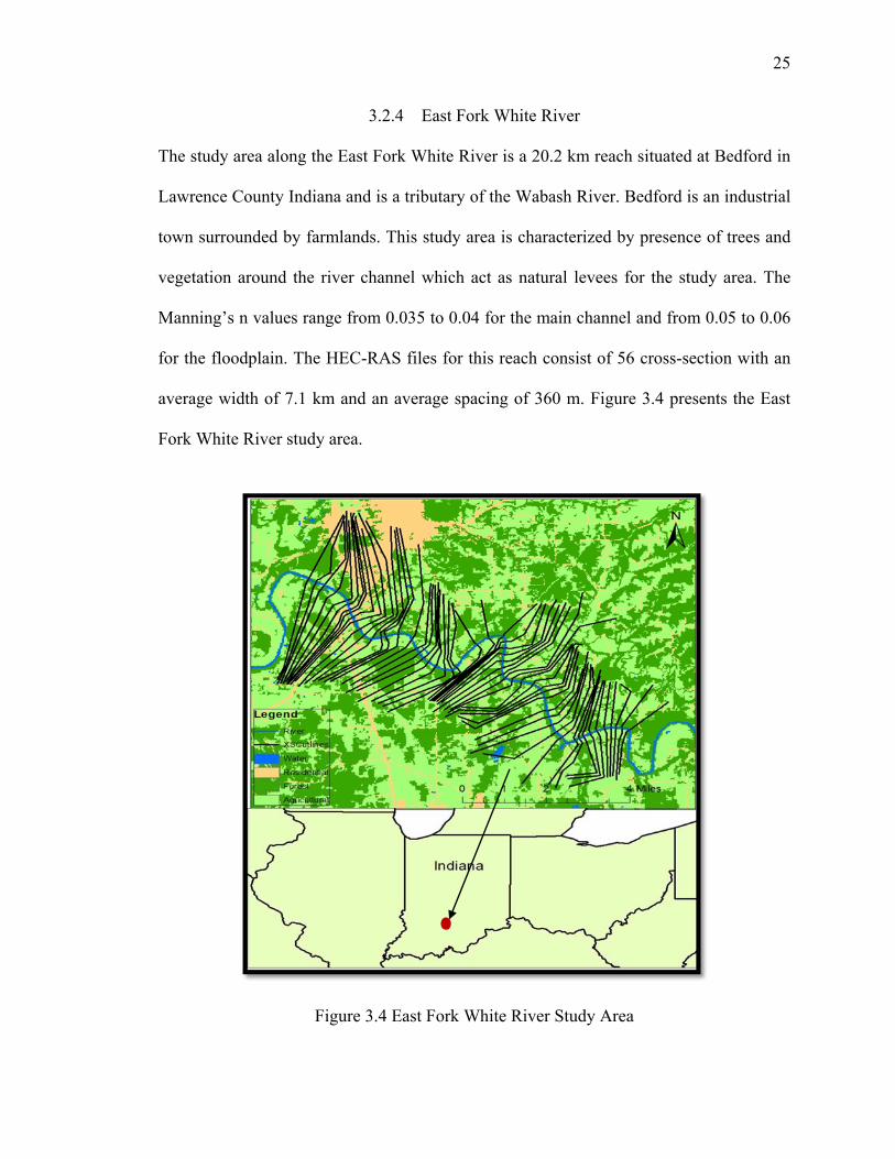
3.2.4 East Fork White River

The study area along the East Fork White River is a 20.2 km reach situated at Bedford in

Lawrence County Indiana and is a tributary of the Wabash River. Bedford is an industrial

town surrounded by farmlands. This study area is characterized by presence of trees and

vegetation around the river channel which act as natural levees for the study area. The

Manning’s n values range from 0.035 to 0.04 for the main channel and from 0.05 to 0.06

for the floodplain. The HEC-RAS files for this reach consist of 56 cross-section with an

average width of 7.1 km and an average spacing of 360 m. Figure 3.4 presents the East

Fork White River study area.

Figure 3.4 East Fork White River Study Area

26

3.2.5 Clear Creek

A 39 km long study area along Clear Creek in Johnson County, Iowa was chosen to account

for variability in Manning’s n values. The entire study area covers two towns: (1) Oxford;

and (2) Coralville. This reach has large cross-sections spanning across 1.5 km to 2 km on

both sides. The average cross-sectional spacing is 452 m and the total number of cross-

sections is 86. The Manning’s n values range from 0.03 to 0.07 along the main channel and

from 0.04 to 0.12 along the floodplain. Figure 3.5 presents the Clear Creek study area.

Figure 3.5 Clear Creek Study Area

27

3.2.6 Brazos River

A 60 km long reach is chosen along Brazos River located in Fort Bend County in Texas

which is the largest reach chosen for this study. This reach has 46 cross-sections with an

average width of 12.2 km and average spacing of 1.3 km. The study area consists of flat

terrain with relatively shallow main channel and meandering bends and thus a significant

amount of flow is routed through the flood plain. Brazos River has recorded major floods

with a significant loss to life and property and in order to protect the areas surrounding this

reach, levees are provided across both sides of the main channel for some regions. The

Manning’s n values range from 0.03 to 0.042 for the main channel and from 0.06 to 0.12

for the floodplain with an agricultural land cover around the area.

Figure 3.6 presents the Brazos River study area.

28

Figure 3.6 Brazos River Study Area

3.3 Description of Flow Data

For this study, 100-year return period flow data is used for hydraulic modeling (Federal

Emergency Management Agency, 2003). The 100-year flow values for Tippecanoe River,

Clear Creek, St. Joseph River and East Fork White River are obtained by modeling the

annual peak flow values obtained from the time series data provided by the United States

Geological Survey (USGS) gage stations.

29

These gage stations were located at the upstream end of the channel reach. Log Pearson

Type III streamflow modeling approach is used to calculate flow values (Hydrology

Subcommittee of U.S. Department of the Interior Geological Survey, 1982). The flow data

for Brazos River is provided by the Fort Bend County and the flow data for Strouds Creek

is provided by the North Carolina Floodplain Mapping Program (NCFMP).

Table 3.1 presents the 100-year steady-state flow rates for all the study areas measured in

cubic meters per second.

Table 3.1 Description of flow data

Study Area 100-year Flow value Station Reach Length (cubic meters/second) (meter) (kilometer)

Strouds Creek 103 6,513.1 6.5 Tippecanoe River 366 10,357.2 10.4 St. Joseph River 606 11,152.2 11.2

East Fork White River 3,673 20,207.3 20.2 Clear Creek 287 39,043.5 39.0

Brazos River 3,061 59,940.9 59.9

3.4 Description of LiDAR Data

Topographic datasets generated using LiDAR data are used for all the study areas. A 6 m

resolution LiDAR for Strouds Creek in North Carolina is provided by NCFMP. The

LiDAR data for four sites viz. Tippecanoe River (3 m resolution), St. Joseph River (3 m

resolution), East Fork White River (3 m resolution) and Clear Creek (1 m resolution)

provided by the USGS Indiana Water Science Center. A 3 m horizontal resolution LiDAR

is provided for the Brazos River by Fort Bend County in Texas.

30

CHAPTER 4. METHODOLOGY

4.1 Introduction

In this chapter, a detailed methodology for calculating water surface elevations and creating

flood inundation maps is presented for the six study areas. Hydraulic/hydrologic modeling

using Geographic Information System (GIS) involves three steps: (1) pre-processing of

data; (2) model execution; and (3) post-processing and visualization of results. Terrain pre-

processing for all the sites is carried out using the HEC-GeoRAS (Ackerman, 2009)

extension within ArcGIS. Flow data are added to the HEC-RAS project files as a part of

model execution and the data obtained through HEC-RAS is exported to ArcGIS for post-

processing to obtain flood maps (Merwade, 2012; Tate & Maidment, 1999). These

processes are repeated for all study areas using different topographic datasets as inputs

during terrain pre-processing.

4.2 Description of 1-D HEC-RAS

HEC-RAS is an open source hydraulic modeling software developed by the United States

Army Corps of Engineers (USACE, 2010) and is used extensively for steady and

unsteady flow modeling in river channels. River reaches generally do not behave as a

single channel which is an assumption for 1-D hydraulic modeling in HEC-RAS.

31

However, during a 100-year flow condition, the main channel and the floodplain act as a

single channel as there are no storage areas in the flood plain and the flow in the flood

plain is parallel to that in the main channel (Jung & Merwade, 2011). Hydraulic

simulations are carried out from one cross-section to the other while the water surface

elevations are interpolated between the two cross sections to generate an entire surface.

Equation 4.1 presents the energy equation used to compute the depth of water for one

cross-section using the depth obtained for another cross-section

Equation 4.1

Where Y1 and Y2 are depths of water from two adjacent cross-sections, Z1 and Z2 are

elevations of the channel invert measure from the datum, V1 and V2 are the average

velocities, α1 and α2 are velocity weighting coefficients, g is the gravitational acceleration

and he is the energy head loss.

The conveyance from the main channel, right overbank and left overbank are calculated

separately and then added to yield the total conveyance. Incremental conveyance values

are obtained using Equation 4.2

Equation 4.2

Where Q is the total conveyance, n is the Manning’s roughness coefficient, R is the

hydraulic radius, A is the flow area and Sf is the slope.

32

Computations in HEC-RAS require geometry data files, upstream flow data and boundary

conditions as input. The geometry data files are exported from ArcGIS for this study and

the boundary conditions are kept constant within a reach for all the topographic datasets.

Wonkovich (2007) emphasized that cross-sections of equal width and similar spacing

should be digitized across the channel to reduce the effects of sudden width changes. The

cross-sections for all the study areas were digitized following this principle.

4.3 Terrain Pre-processing using ArcGIS

This step is carried out to create the geometry files which are used as input in HEC-RAS

where the hydraulic modeling takes place. Topographic datasets are used to extract

elevations for river centerline, bank lines, flow paths, bridges and cross-sections. These

features are digitized within ArcGIS using the HEC-GeoRAS extension.

Cross-sections are cut across the entire reach to capture all inundated areas since modeling

is carried out for 100-year flows and may result in water being predicted as inundated

outside the floodplain. DEMs and aerial photographs of the study area are overlaid and

used as spatial reference to create the river centerline, flow paths, banks, bridges and cross-

section layers. Two cross-sections are placed both upstream and downstream of bridges. In

addition to these features, areas representing zero flow velocity called ineffective flow

areas and regions with no flow and water called blocked obstructions are digitized using

aerial photographs (Merwade, 2012).

33

Figure 3.7, Figure 3.8 and Figure 3.9 show the terrain pre-processing maps for all the study

areas.

Figure 3.7 Terrain Pre-Processing for Strouds Creek and Tippecanoe River

34

Figure 3.8 Terrain Pre-processing for St. Joseph River and East Fork White River

35

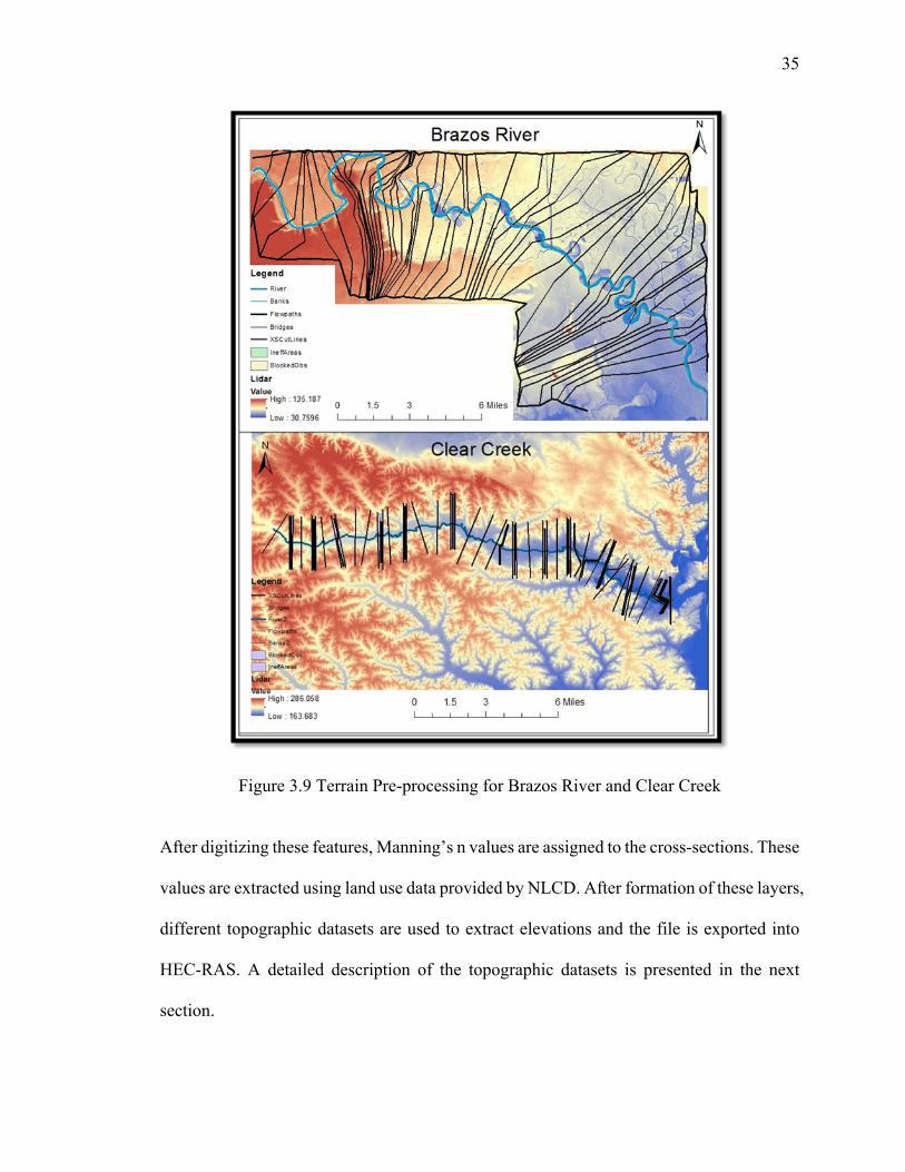
Figure 3.9 Terrain Pre-processing for Brazos River and Clear Creek

After digitizing these features, Manning’s n values are assigned to the cross-sections. These

values are extracted using land use data provided by NLCD. After formation of these layers,

different topographic datasets are used to extract elevations and the file is exported into

HEC-RAS. A detailed description of the topographic datasets is presented in the next

section.

36

4.4 Description of Topographic Datasets

To understand the relationship between grid size and DEM errors with water surface

elevations and flood extents, different topographic datasets are used to extract elevations

using HEC-GeoRAS in ArcGIS. This leads to creation of geometry files with different

elevations for river centerline, cross-sections, flow lines, bridges, ineffective flow areas

and blocked obstructions. The methodology to establish the relationship between DEM

resolution and hydraulic outputs is described in Section 4.3.1 and the relationship between

DEM errors and hydraulic outputs is discussed in Section 4.3.2.

4.4.1 Effect of DEM Resolution on Hydraulic Outputs

The original LiDAR dataset is resampled into different grid sizes using the Data

Management Toolbox in ArcGIS for all the study areas. Resampling is a technique of

changing the proportions of a discrete raster into a continuous raster and subsequently

interpolating it into a discrete raster of different grid size (Parker et al., 1983).

Resampling datasets into larger grid sizes often leads to loss in quality and accuracy of the

dataset. Resampling in ArcGIS can be done through three methods: (1) nearest neighbor;

(2) bilinear; and (3) cubic. For this analysis, the nearest neighbor technique is used which

assigns the new point a value equal to that of its nearest neighbor. This technique is useful

since it does not change the original elevations of the existing points (Simon, 1975).

For Strouds Creek, the original 6 m resolution LiDAR is resampled into different grid sizes

of 9-, 12-, 15-, 18-, 21-, 24-, 27-, 30-, 33-, 36-, 48-, 60-, 70-, 80-, 90- and 100 m.

37

These DEMs are used to extract elevations into different layers using HEC-GeoRAS and

then export these layers into HEC-RAS to create 17 geometry files including the original

LiDAR. For Tippecanoe River, the original 3 m resolution LiDAR is resampled to generate

DEMs of grid size 6-, 9-, 12-, 15-, 18-, 21-, 24-, 27-, 30-, 33-, 36-, 48-, 60-, 70-, 80-, 90-

and 100 m thus creating 18 geometry files. Similarly, 18 geometry files are created for St.

Joseph River, Brazos River and East Fork White River using the 3 m resolution LiDAR

DEMs.

4.4.2 Effect of DEM Error on Hydraulic Outputs

Root Mean Squared Error (RMSE) is a widely used statistic for measuring the error

between actual and estimated values. It is used to report a single global value of error in

elevations for the entire DEM (Fisher & Tate, 2006). For this study, RMSE is used to

evaluate the difference in accuracy between the original LiDAR data and its resampled

DEMs. It should be noted that the cause of error in DEMs is not limited to resampling

errors. However, this study aims to quantify the amount of error occurring in different

DEMs and understand how these errors effect the overall estimation of hydraulic outputs.

The RMSE is calculated as the square root of the sum of squares of elevation difference

between the resampled DEM and the original LiDAR for each point divided by the total

number of points (Z. Li, 1988). This analysis shows the variation of RMSE with grid size.

The RMSE values are calculated using the following equation

∑ Equation 4.3

38

Where Zil is the elevation value for the ith point extracted from a LiDAR DEM, Zir is the

elevation value for the ith point extracted from a resampled DEM, n is the total number of

points for which elevation values are extracted and RMSEr is the root mean squared error

for a resampled DEM when compared to a LiDAR DEM. To analyze these DEMs, a point

shape file is overlay on the base (LiDAR) dataset and elevation values are extracted to each

point in the shape file using the base DEM. This process is carried out for the same points

representing elevations corresponding to different resolution resampled datasets.

A Root Mean Squared Error (RMSE) comparison of DEMs is an appropriate way of error

estimation. However, since RMSE results in only one value per DEM, it is essential to

measure the spatial variability. This analysis involves adding these RMSE values to the

original LiDAR DEM to understand the effect of adding errors to a DEM. This analysis is

carried out because the DEMs contain errors due to other factors apart from resolutions.

For Strouds Creek study area, random raster datasets containing errors are created using

the RMSE values and added to the original raster using the Raster Calculator in ArcGIS.

DEM accuracy measurements standards are provided in a document called “National

Standards for Spatial Data Accuracy” (NSSDA) published by the US Federal Geographic

Data Committee (FGDC, 1998). These guidelines state that the DEM errors follow a

normal distribution. For an open terrain, a normal distribution of error is a fair assumption

and the residual errors lie within 95 % confidence intervals (Flood, 2004).

39

Using these guidelines, past studies on estimating the accuracy of DEMs have assumed a

normal distribution of errors (Aguilar et al., 2007), however, this assumption does not hold

true for non-open terrain for which the error distribution not normal and the effect of

outliers is significant (Aguilar et al., 2008). The random error datasets for this study are

also created using normal distribution assumption with the mean of the distribution equal

to the RMSE. The standard deviation (SD) for these raster datasets is calculated by

selecting a set of points in the flood plain. The standard deviations in elevations

corresponding to these set of points are used in creating the normal error datasets (Aguilar

et al., 2005).

The datasets are also resampled to 9-, 12-, 15-, 18-, 21-, 24-, 27-, 30-, 36-, 48-, 60- and 80

m and added to the resampled DEMs. Thus the new DEMs are resampled and also contain

errors. Using this approach, 12 variations of the original LiDAR datasets are obtained

which contain normal errors equal to RMSE values obtained from all the resampled DEMs

of Strouds Creek. After creation of all the topographic datasets and creation of geometry

files, hydraulic modeling is carried out in HEC-RAS which is described in Section 4.4.

4.5 Hydraulic Modeling using 1-D HEC-RAS

Resampled DEMs including LiDAR resulted in 18 different geometry files for St. Joseph

River, Tippecanoe River, East Fork White River and Brazos River while 17 geometry files

were created for Strouds Creek. Thus a total of 89 geometry files were created to measure

the effect of grid size on hydraulic outputs. Twelve additional geometry files were created

to by adding normal errors for Strouds Creek.

40

Thus, a total of 101 hydraulic simulations were run for six study areas. The 100-year flow

values were used as steady-flow input into HEC-RAS. All the other data including

boundary conditions, ineffective flow areas, land use and blocked obstructions remain

unchanged for all simulations within a reach. Since HEC-RAS permits the use of only 500

points for a given cross-section, the number of points across every cross-section were

filtered using the cross-section filter tool in HEC-RAS. The obtained water surface

elevations were exported into ArcGIS for creating flood maps.

4.6 Creation of Flood Maps

The HEC-RAS output file is imported into ArcGIS using HEC-GeoRAS for creating flood

inundation maps. The topographic datasets are subtracted from Triangular Irregular

Networks (TIN) created using the water surface elevations resulting in a water depth raster.

The areas with water depth less than zero are removed to obtain a flood depth map. The

areas with water depth greater than zero are considered to be flooded (Merwade, 2012;

Noman et al., 2001; Omer et al., 2003; Tate et al., 2002). The area of flood extent is

calculated by converting the flood depth raster into a polygon shape file and adding the

areas of all the polygons. The flood inundation area values are exported into Excel to

analyze the effect of grid size and DEM errors.

41

CHAPTER 5. RESULTS

5.1 Introduction

The results from hydraulic modeling using HEC-RAS and flood inundation mapping using

HEC-RAS outputs in ArcGIS are presented in this chapter. To establish a relationship

between hydraulic outputs and grid size, average water surface elevations and flood

inundation extents for all the study areas are presented. The average water surface

elevations have been calculated as an average of all cross-section station across the entire

channel.

Inundation area refers to the total area predicted as inundated and is calculated by adding

the total number of inundated cells and multiplying by the area of one cell. The percentage

change in inundation area is presented using the original LiDAR DEM generated results as

base values. These values are also presented for 12 topographic datasets containing errors

for Strouds Creek to analyze the effect of DEM errors on average water surface elevations

and inundation area.

5.2 Effect of DEM Resolution on Hydraulic Outputs

The first objective of this study is to determine a relationship between DEM resolution and

flood inundation mapping.

42

This relationship can be applied to other coarser DEMs where LiDAR data is unavailable.

The study areas are classified into two different groups based on the land use characteristics

and size to account for different characteristics. Strouds Creek, Tippecanoe River and St.

Joseph River are study areas with urban land use and small size. East Fork White River

and Brazos River are large study areas with agricultural and forest land use. The water

surface elevations, flood inundation area and percentage change in inundation area for all

the topographic datasets are evaluated and compared with the grid sizes. For each study

area, cross-sections along one station are presented for the original LiDAR and a 100 m

resolution resampled DEM.

5.2.1 Study Areas with small size and urban land use

Table 5.1 presents the average water surface elevations (WS El.), inundation area and

percentage change in inundated area for DEMs of increasing grid size or decreasing

resolution for the Strouds Creek study area.

43

Table 5.1 Hydraulic outputs for Strouds Creek

Grid Size Avg. WS El. Inundation

Area % change

(meter) (meter) (km2)

6 (LiDAR) 164.276 0.363 0.00 9 164.343 0.372 2.42 12 164.398 0.389 7.00 15 164.543 0.393 8.19 18 164.601 0.403 10.85 21 164.743 0.421 15.76 24 164.815 0.421 15.97 27 164.943 0.447 23.00 30 165.070 0.441 21.33 33 165.194 0.481 32.35 36 165.348 0.492 35.45 48 165.786 0.523 43.84 60 166.308 0.604 66.36 70 166.669 0.613 68.86 80 166.750 0.687 89.22 90 167.290 0.703 93.52

100 167.240 0.635 74.79

The results of the table show that water surface elevations increase with increasing grid

size. The LiDAR DEM has a water surface elevation of 164.2 m while the 100 m grid size

DEM has a water surface elevation of 167.2 m thus a difference of about 3 m is observed.

A similar trend occurred for inundation area with about 74.8 % rise in the inundated area

from a LiDAR DEM to a 100 m resolution DEM.

The results of hydraulic modeling and flood inundation mapping for Tippecanoe River

study area are presented in Table 5.2.

44

Table 5.2 Hydraulic outputs for Tippecanoe River

Grid Size Avg. WS El. Inundation

Area % change

(meter) (meter) (km2)

3 (LiDAR) 210.902 2.937 0.00 6 210.915 2.942 0.17 9 210.935 2.957 0.68 12 210.976 2.975 1.31 15 210.986 2.997 2.05 18 210.845 2.880 -1.95 21 211.058 3.012 2.55 24 211.073 3.051 3.88 27 211.055 3.047 3.73 30 211.065 3.031 3.20 33 211.171 3.100 5.56 36 211.335 3.242 10.39 48 211.310 3.243 10.40 60 211.396 3.343 13.82 70 211.652 3.562 21.28 80 211.753 3.795 29.20 90 212.042 4.261 45.08

100 212.029 4.189 42.63

The water surface elevations increase with grid size for Tippecanoe River as well. The

original 3 m LiDAR DEM predicts a water surface elevation of 210.9 m while the 100 m

resolution DEM has a water surface elevation of 212.0 m with difference of about 1.1 m.

The percentage change in inundation area is not significant up to a resolution of about 33

m but a change in inundation area of about 42.63 % occurs for a 100 m resolution DEM.

Table 5.3 presents the average water surface elevations, inundation area and percent

inundated for the St. Joseph River study area.

45

Table 5.3 Hydraulic outputs for St. Joseph River

Grid Size Avg. WS El. Inundation

Area % change

(meter) (meter) (km2)

3 (LiDAR) 221.275 3.156 0.00 6 221.316 3.198 1.34 9 221.329 3.206 1.61 12 221.470 3.298 4.50 15 221.408 3.263 3.39 18 221.434 3.297 4.48 21 221.457 3.331 5.55 24 221.506 3.391 7.46 27 221.561 3.392 7.48 30 221.545 3.397 7.65 33 221.589 3.489 10.56 36 221.568 3.384 7.23 48 221.761 3.640 15.35 60 221.893 3.698 17.18 70 221.973 3.805 20.59 80 222.211 3.950 25.16 90 221.927 3.739 18.47

100 222.017 3.851 22.04

The results from hydraulic modeling for St. Joseph River show that there is difference of

0.75 m between the water surface elevations generated from LiDAR and 100 m DEM. The

percentage change in the inundated area between LiDAR and 100 m DEM is 22.04 %

which is smaller than the percentage change observed form Strouds Creek and Tippecanoe

River. This is because St. Joseph River has deeper and wider cross-sections thus the

majority of the water is conveyed through the channel itself and only some of it passes

through the flood plain.

46

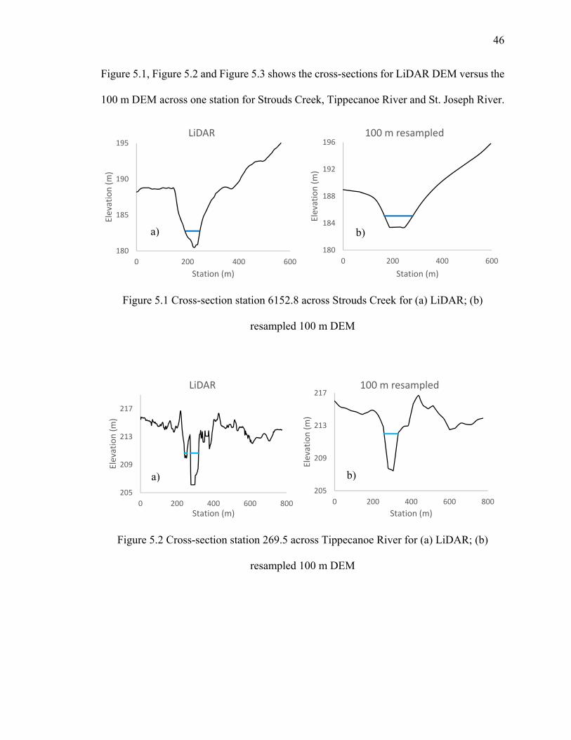
Figure 5.1, Figure 5.2 and Figure 5.3 shows the cross-sections for LiDAR DEM versus the

100 m DEM across one station for Strouds Creek, Tippecanoe River and St. Joseph River.

Figure 5.1 Cross-section station 6152.8 across Strouds Creek for (a) LiDAR; (b)

resampled 100 m DEM

Figure 5.2 Cross-section station 269.5 across Tippecanoe River for (a) LiDAR; (b)

resampled 100 m DEM

180

185

190

195

0 200 400 600

Elevation (m)

Station (m)

LiDAR

180

184

188

192

196

0 200 400 600

Elevation (m)

Station (m)

100 m resampled

205

209

213

217

0 200 400 600 800

Elevation (m)

Station (m)

LiDAR

205

209

213

217

0 200 400 600 800

Elevation (m)

Station (m)

100 m resampled

a) b)

b)a)

47

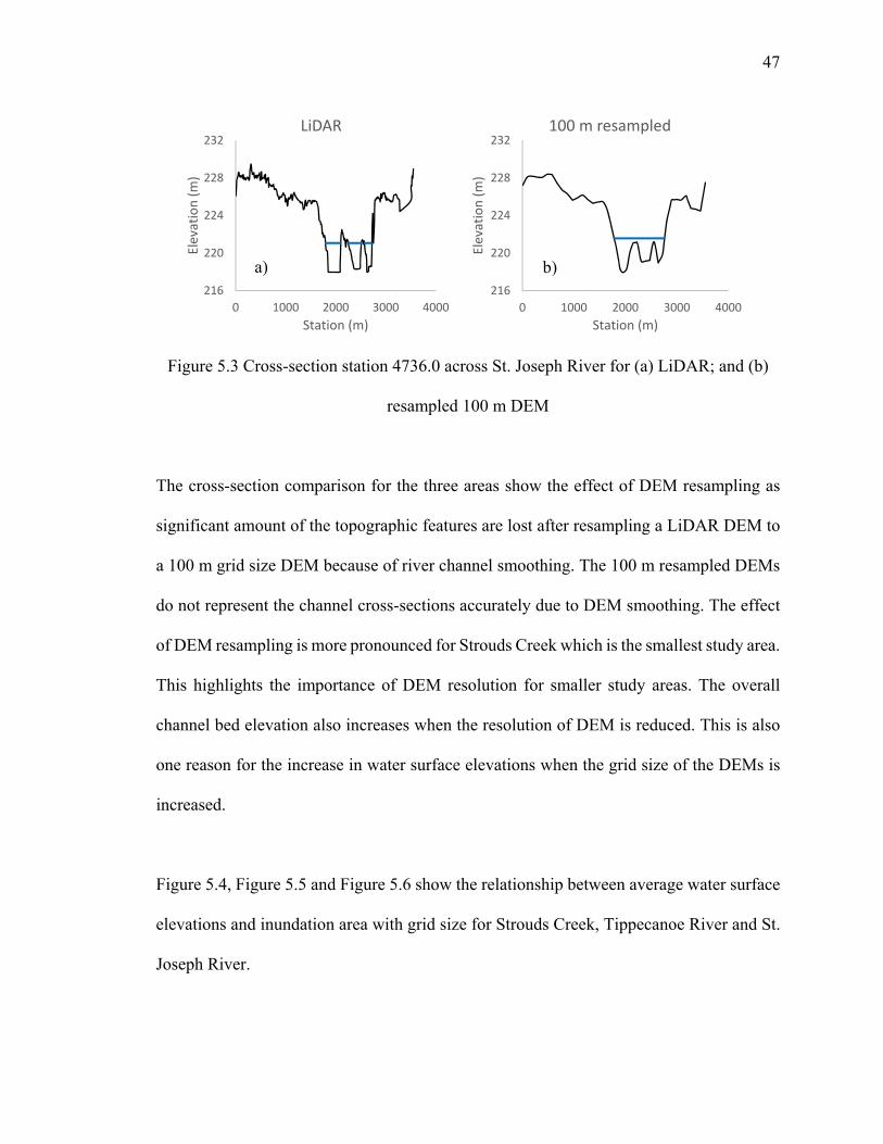
Figure 5.3 Cross-section station 4736.0 across St. Joseph River for (a) LiDAR; and (b)

resampled 100 m DEM

The cross-section comparison for the three areas show the effect of DEM resampling as

significant amount of the topographic features are lost after resampling a LiDAR DEM to

a 100 m grid size DEM because of river channel smoothing. The 100 m resampled DEMs

do not represent the channel cross-sections accurately due to DEM smoothing. The effect

of DEM resampling is more pronounced for Strouds Creek which is the smallest study area.

This highlights the importance of DEM resolution for smaller study areas. The overall

channel bed elevation also increases when the resolution of DEM is reduced. This is also

one reason for the increase in water surface elevations when the grid size of the DEMs is

increased.

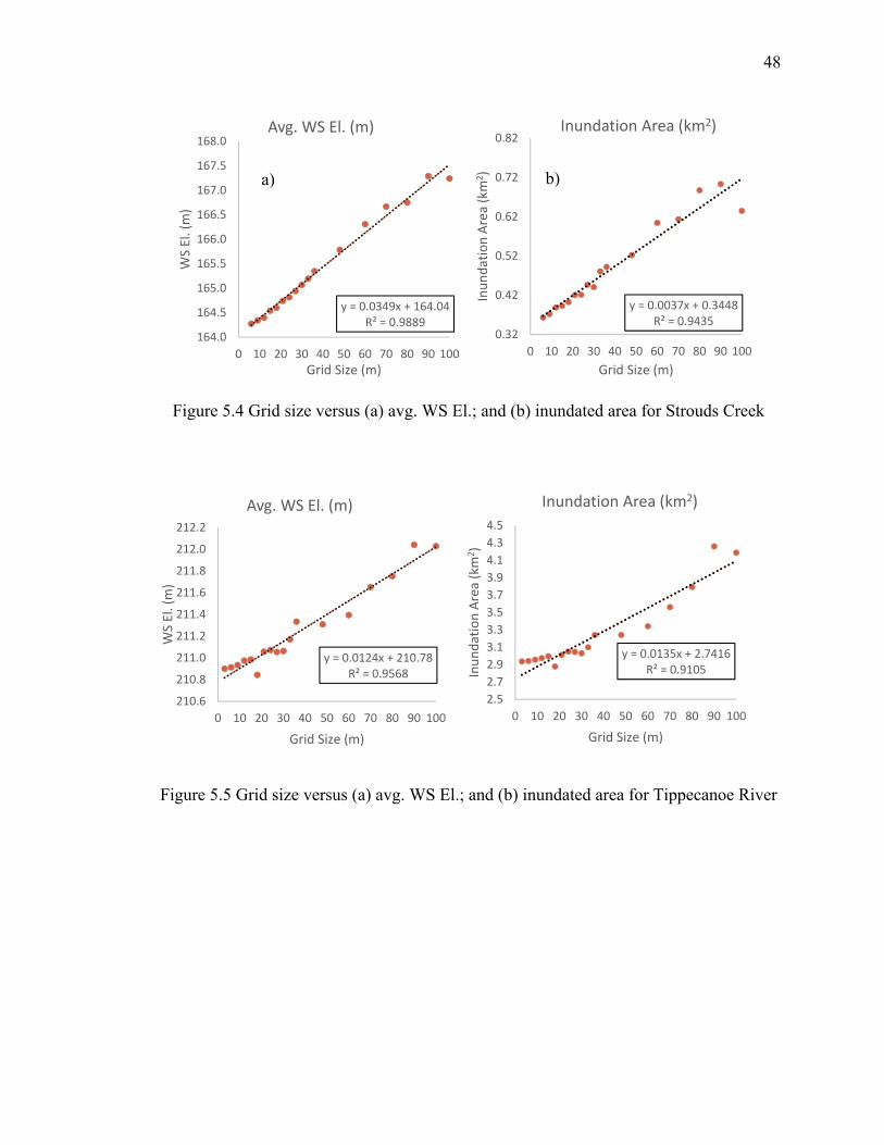
Figure 5.4, Figure 5.5 and Figure 5.6 show the relationship between average water surface

elevations and inundation area with grid size for Strouds Creek, Tippecanoe River and St.

Joseph River.

216

220

224

228

232

0 1000 2000 3000 4000

Elevation (m)

Station (m)

LiDAR

216

220

224

228

232

0 1000 2000 3000 4000

Elevation (m)

Station (m)

100 m resampled

a) b)

48

Figure 5.4 Grid size versus (a) avg. WS El.; and (b) inundated area for Strouds Creek

Figure 5.5 Grid size versus (a) avg. WS El.; and (b) inundated area for Tippecanoe River

y = 0.0349x + 164.04R² = 0.9889

164.0

164.5

165.0

165.5

166.0

166.5

167.0

167.5

168.0

0 10 20 30 40 50 60 70 80 90 100

WS El. (m)

Grid Size (m)

Avg. WS El. (m)

y = 0.0037x + 0.3448R² = 0.9435

0.32

0.42

0.52

0.62

0.72

0.82

0 10 20 30 40 50 60 70 80 90 100

Inundation Area (km

2)

Grid Size (m)

Inundation Area (km2)

y = 0.0124x + 210.78R² = 0.9568

210.6

210.8

211.0

211.2

211.4

211.6

211.8

212.0

212.2

0 10 20 30 40 50 60 70 80 90 100

WS El. (m)

Grid Size (m)

Avg. WS El. (m)

y = 0.0135x + 2.7416R² = 0.9105

2.5

2.7

2.9

3.1

3.3

3.5

3.7

3.9

4.1

4.3

4.5

0 10 20 30 40 50 60 70 80 90 100

Inundation Area (km

2)

Grid Size (m)

Inundation Area (km2)

a) b)

49

Figure 5.6 Grid size versus (a) avg. WS El.; and (b) inundated area for St. Joseph River

The results clearly show that both average water surface elevations and inundation area

have a linear relationship with grid size for all three study areas. The predicted linear

equations between average water surface elevations and grid size have an R2 greater than

90 % for the three study areas. The inundated area is also related to grid size with a linear

equation with R2 greater than 90 % for the three reaches. The high R2 values suggest a very

good linear fit between hydraulic outputs and DEM resolution.

There were some anomalies in the water surface elevations and predicted areas for the 90

m resolution DEM for St. Joseph River. This could be due to the presence of certain areas

for which more than one cell was inundated for a 90 m DEM while only one cell was

inundated for a 100 m DEM because of a slight change in elevation during resampling.

y = 0.0087x + 221.3R² = 0.9057

221.2

221.4

221.6

221.8

222.0

222.2

222.4

0 10 20 30 40 50 60 70 80 90 100

WS El. (m)

Grid Size (m)

Avg. WS El. (m)

y = 0.0079x + 3.174R² = 0.9162

3.00

3.20

3.40

3.60

3.80

4.00

4.20

0 10 20 30 40 50 60 70 80 90 100

Inundation Area (km

2)

Grid Size (m)

Inundation Area (km2)

50

Figure 5.7, Figure 5.8 and Figure 5.9 present the comparison between flood inundation

maps for Strouds Creek, Tippecanoe River and St. Joseph River created using (a) original

LiDAR; (b) 30 m resampled DEM; (c) 60 m resampled DEM; and (d) 100 m resampled

DEM.

Figure 5.7 Flood maps generated from different resolution DEMs for Strouds Creek

51

Figure 5.8 Flood maps generated from different resolution DEMs for Tippecanoe River

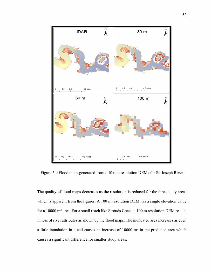
52

Figure 5.9 Flood maps generated from different resolution DEMs for St. Joseph River

The quality of flood maps decreases as the resolution is reduced for the three study areas

which is apparent from the figures. A 100 m resolution DEM has a single elevation value

for a 10000 m2 area. For a small reach like Strouds Creek, a 100 m resolution DEM results

in loss of river attributes as shown by the flood maps. The inundated area increases as even

a little inundation in a cell causes an increase of 10000 m2 in the predicted area which

causes a significant difference for smaller study areas.

53

The flood maps generated using DEMs of different resolutions clearly show that for a small

study area like Strouds Creek, a higher resolution DEM best represents the terrain and

predicts more precise flood maps. The 100 m DEM flood maps is just a scattered set of

cells showing inundation while the LiDAR represents the extent of flooding across the river

channel and the floodplain in the best manner.

There is no significant variation between the flood maps generated from LiDAR and 30 m

resolution DEMs for Tippecanoe River and St. Joseph River. The 60 m and 100 m

resolution DEMs predict inundated areas which are not predicted as inundated using the

LiDAR and 30 m DEM. The flood maps obtained from a 100 m DEM do not give an

appropriate description of river and flood plain morphology.

5.2.2 Study Areas with large size and agricultural land use

East Fork White River and Brazos River are comparatively bigger reaches with wider and

deeper channels as compared to Strouds Creek, Tippecanoe River and St. Joseph River.

Both these reaches have an agricultural land use with flat flood plains. Brazos River is

characterized by presence of levees for downstream end of the study area while East Fork

White River has large trees and vegetation around the main channel which act as natural

levees.

Table 5.4 presents the hydraulic outputs versus grid size for East Fork White River.

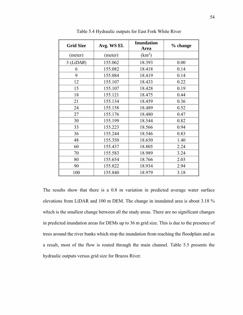
54

Table 5.4 Hydraulic outputs for East Fork White River

Grid Size Avg. WS El. Inundation

Area % change

(meter) (meter) (km2)

3 (LiDAR) 155.062 18.393 0.00 6 155.082 18.418 0.14 9 155.084 18.419 0.14 12 155.107 18.433 0.22 15 155.107 18.428 0.19 18 155.121 18.475 0.44 21 155.134 18.459 0.36 24 155.158 18.489 0.52 27 155.176 18.480 0.47 30 155.199 18.544 0.82 33 155.223 18.566 0.94 36 155.244 18.546 0.83 48 155.350 18.650 1.40 60 155.437 18.805 2.24 70 155.583 18.989 3.24 80 155.654 18.766 2.03 90 155.822 18.934 2.94

100 155.840 18.979 3.18

The results show that there is a 0.8 m variation in predicted average water surface

elevations from LiDAR and 100 m DEM. The change in inundated area is about 3.18 %

which is the smallest change between all the study areas. There are no significant changes

in predicted inundation areas for DEMs up to 36 m grid size. This is due to the presence of

trees around the river banks which stop the inundation from reaching the floodplain and as

a result, most of the flow is routed through the main channel. Table 5.5 presents the

hydraulic outputs versus grid size for Brazos River.

55

Table 5.5 Hydraulic outputs for Brazos River

Grid Size Avg. WS El. Inundation

Area % change

(meter) (meter) (km2)

3 (LiDAR) 22.727 162.290 0.00 6 22.726 162.304 0.01 9 22.747 164.349 1.27 12 22.749 164.436 1.32 15 22.771 166.159 2.38 18 22.779 166.942 2.87 21 22.791 169.248 4.29 24 22.808 169.304 4.32 27 22.824 170.628 5.14 30 22.832 172.388 6.22 33 22.841 174.112 7.28 36 22.905 177.916 9.63 48 22.922 177.580 9.42 60 22.983 181.818 12.03 70 23.018 184.665 13.79 80 23.116 188.506 16.15 90 23.066 190.101 17.14

100 23.201 191.924 18.26

The results for Brazos River show that water surface elevations do not change significantly

with grid size for Brazos River with a difference of only 0.5 m between results obtained

from LiDAR and 100 m DEM. This is due to the relatively flat floodplain for Brazos River.

Since the river channel is not too deep, most of the water flows through the floodplain

resulting in larger flood extents and less variation in water surface elevations. The

inundation area however, increases significantly on increasing grid size with a change of

18.26 % between the predicted inundation values between LiDAR and the 100 m DEM.

56

Figure 5.10 and Figure 5.11 show the comparison between LiDAR and 100 m DEM for

one cross-sections station across East Fork White River and Brazos River.

Figure 5.10 Cross-section Station 19206.5 across East Fork White River for (a) LiDAR;

(b) resampled 100m DEM

Figure 5.11 Cross-section station 33160.7 across Brazos River for (a) LiDAR; and (b)

resampled 100 m DEM

The study area for East Fork White River has natural levees around it which results in less

variation in the extent of inundation. The main channel is deeper and smoother than the

other reaches and thus the effect of resampling is not significant for the main channel.

140

150

160

170

180

190

200

210

220

0 1000 2000 3000 4000 5000

Elevation (m)

Station (m)

LIDAR

GroundStation

WS 100‐yr

140

150

160

170

180

190

200

210

220

0 1000 2000 3000 4000 5000

Elevation (m)

Station (m)

100 m Resampled DEM

GroundStation

WS 100‐yr

12

14

16

18

20

22

24

26

28

0 2000 4000 6000 8000

Elevation (m)

Station (m)

LiDAR

GroundStation

WS 100‐yr

12

14

16

18

20

22

24

26

28

0 2000 4000 6000 8000

Elevation (m)

Station (m)

100 m re‐sampled

GroundStation

WS 100‐yr

a) b)

a) b)

57

Since the floodplain is characterized by presence of trees, the overall difference in

predicted water surface elevations is also less between the LiDAR and 100 m DEM.

The width of the cross-sections for Brazos River is about 7.6 km and there is a significant

smoothing effect of the old stream beds and ridges for such a large reach. Figure 5.11 shows

that three small channel regions which were present in the LiDAR cross-section are

converted into a single channel for a 100 m DEM. However, the overall profile of the cross-

section does not change much because even for a 100 m DEM, the width of the cross-

section is much more than the horizontal resolution, the channel terrain is represented fairly

even with a 100 m DEM.

Figure 5.12 and Figure 5.13 shows the relationship between grid size and hydraulic outputs

for East Fork White River and Brazos River.

Figure 5.12 Grid size versus (a) avg. WS El.; and (b) inundated area for White River

y = 0.0085x + 154.98R² = 0.9785

154.8

155.0

155.2

155.4

155.6

155.8

156.0

0 10 20 30 40 50 60 70 80 90 100

WS El. (m)

Grid Size (m)

Avg. WS El. (m)

y = 0.0066x + 18.35R² = 0.9216

18.3

18.4

18.5

18.6

18.7

18.8

18.9

19.0

19.1

0 10 20 30 40 50 60 70 80 90 100

Inundation Area (km

2)

Grid Size (m)

Inundation Area (km2)

a) b)

58

Figure 5.13 Grid size versus (a) avg. WS El.; and (b) inundated area for Brazos River

There is a linear relationship between average water surface elevations and grid size even

for larger study areas such as East Fork White River and Brazos River as shown by high

R2 values greater than 95 %. The inundation area is also linearly related with grid size with

R2 greater than 90 %. The variations in land use types also does not affect the linear

relationship significantly suggested by the fact that this relationship is true for Strouds

Creek and St. Joseph River study areas which have an urban land use and East Fork White

River and Brazos river which have a relatively flat and agricultural floodplain.

Figure 5.14 presents a comparison of flood maps generated using (a) LiDAR; (b) 30 m; (c)

60 m; and (d) 100 m DEMs for a part of East Fork White River.

y = 0.0047x + 22.699R² = 0.9775

22.6

22.7

22.8

22.9

23.0

23.1

23.2

23.3

0 10 20 30 40 50 60 70 80 90 100

WS El. (m)

Grid Size (m)

Avg. WS El. (m)

y = 0.3219x + 161.95R² = 0.9783

159.0

164.0

169.0

174.0

179.0

184.0

189.0

194.0

199.0

0 10 20 30 40 50 60 70 80 90 100

Inundation Area (km

2)

Grid Size (m)

Inundation Area (km2)

b)a)

59

Figure 5.14 Flood maps generated from different resolution DEMs for White River

The predicted inundation extents for East Fork White River do not change significantly.

This is also due to presence of trees around the main channel and existence of deeper

channels which route most of the flow thus producing flood maps representing the

inundated areas fairly well even for larger DEMs.

Figure 5.15 presents a comparison of flood maps generated using (a) LiDAR; (b) 30 m; (c)

60 m; and (d) 100 m DEMs for a part of Brazos River.

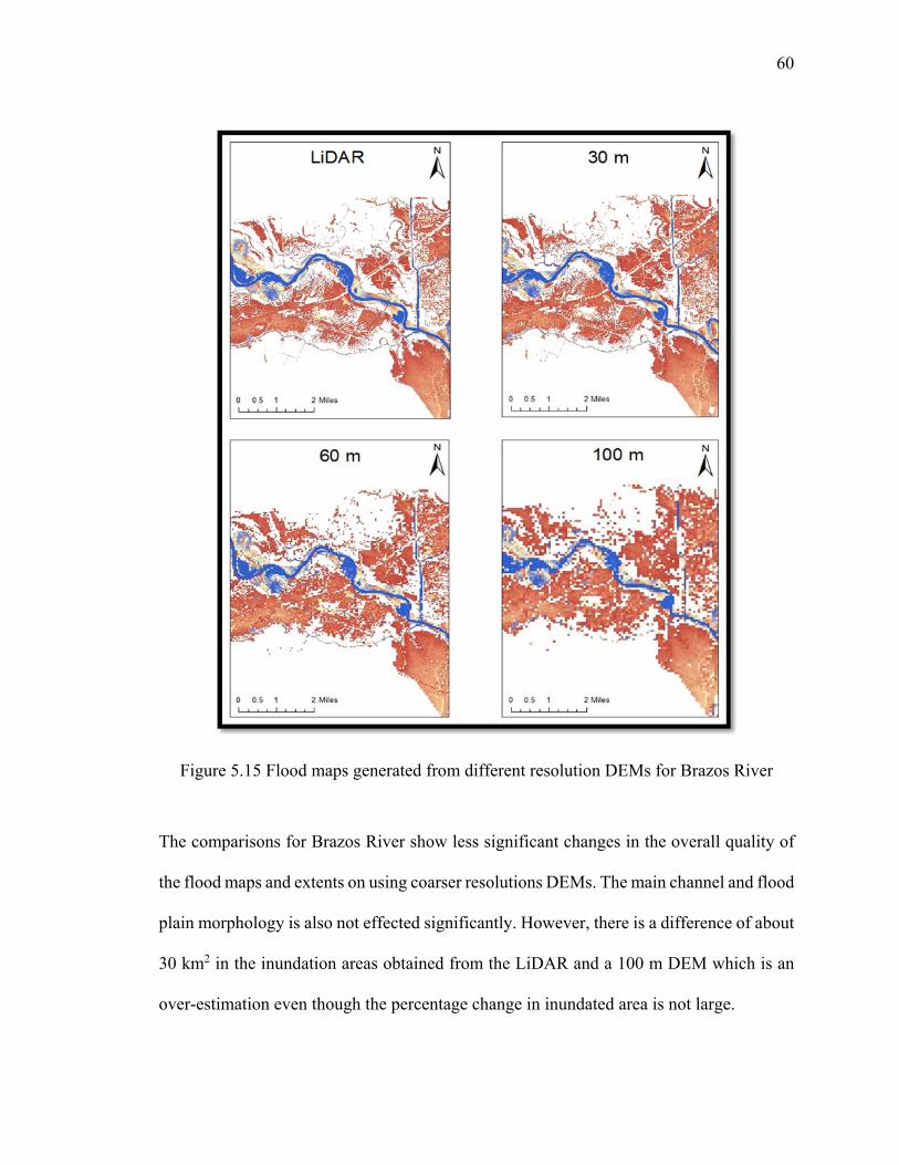
60

Figure 5.15 Flood maps generated from different resolution DEMs for Brazos River

The comparisons for Brazos River show less significant changes in the overall quality of

the flood maps and extents on using coarser resolutions DEMs. The main channel and flood

plain morphology is also not effected significantly. However, there is a difference of about

30 km2 in the inundation areas obtained from the LiDAR and a 100 m DEM which is an

over-estimation even though the percentage change in inundated area is not large.

61

5.3 Effect of DEM Error on Hydraulic Outputs

5.3.1 RMSE of Elevations versus Grid Size

To measure the amount of error present in the resampled DEMs with respect to the original

LiDAR DEMs, RMSE for different grid sizes of DEMs is presented below. This estimation

has been carried out for Tippecanoe River, St. Joseph River and Strouds Creek because of

the urban land use and terrain with high slope. The results for RMSE versus grid size are

shown in Table 5.6.

Table 5.6 RMSE versus grid size

Strouds Creek Tippecanoe River St. Joseph River Grid Size RMSE RMSE RMSE

(m) (m) (m) (m) 6 0.166 0.145 9 0.348 0.190 0.167 12 0.424 0.262 0.230 15 0.467 0.294 0.261 18 0.489 0.350 0.306 21 0.608 0.385 0.338 24 0.692 0.437 0.380 27 0.749 0.462 0.404 30 0.798 0.440 36 0.961 48 1.211 60 1.481 80 1.879

The results show that RMSE values for the three study areas show that RMSE values are

directly related to the shape and slope of the valley since Strouds Creek had the largest

RMSE and the highest slope.

62

The size of the study area also affected the RMSE values since it is directly related to the

number of points chosen for analysis in the flood plain as the RMSE values were calculated

for the entire topographic dataset. The number of points for which RMSE values were

calculated were 160,238 for Strouds Creek, 1,865,634 for Tippecanoe River and 5,044,902

for St. Joseph River. The magnitude of RMSE decreases when the number of points are

increased.

The RMSE for the 9 m DEM was reported as 0.347 m for Strouds Creek, 0.19 m for

Tippecanoe River and 0.167 m for St. Joseph River. These values clearly show that the

global RMSE values decrease on increasing the size of the topographic dataset. This can

be explained because the maximum error in elevations for DEMs occurs in measuring the

river main channel elevations. The percentage area of the river in the DEM for Strouds

Creek is higher than Tippecanoe River and St. Joseph River hence the RMSE is also high.

Figure 5.16 shows the relationship between RMSE and grid size for St. Joseph River,

Tippecanoe River and Strouds Creek.

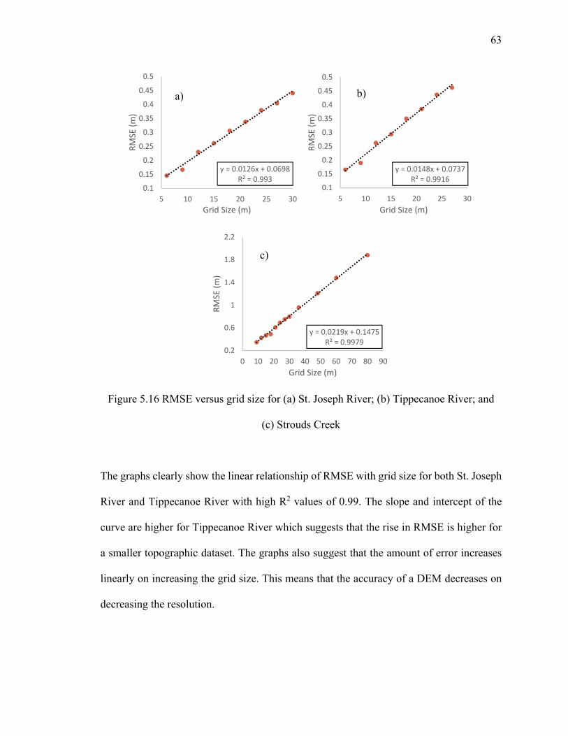
63

Figure 5.16 RMSE versus grid size for (a) St. Joseph River; (b) Tippecanoe River; and

(c) Strouds Creek

The graphs clearly show the linear relationship of RMSE with grid size for both St. Joseph

River and Tippecanoe River with high R2 values of 0.99. The slope and intercept of the

curve are higher for Tippecanoe River which suggests that the rise in RMSE is higher for

a smaller topographic dataset. The graphs also suggest that the amount of error increases

linearly on increasing the grid size. This means that the accuracy of a DEM decreases on

decreasing the resolution.

y = 0.0126x + 0.0698R² = 0.993

0.1

0.15

0.2

0.25

0.3

0.35

0.4

0.45

0.5

5 10 15 20 25 30

RMSE (m)

Grid Size (m)

y = 0.0148x + 0.0737R² = 0.9916

0.1

0.15

0.2

0.25

0.3

0.35

0.4

0.45

0.5

5 10 15 20 25 30

RMSE (m)

Grid Size (m)

y = 0.0219x + 0.1475R² = 0.9979

0.2

0.6

1

1.4

1.8

2.2

0 10 20 30 40 50 60 70 80 90

RMSE (m)

Grid Size (m)

a) b)

c)

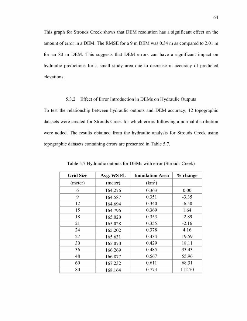
64

This graph for Strouds Creek shows that DEM resolution has a significant effect on the

amount of error in a DEM. The RMSE for a 9 m DEM was 0.34 m as compared to 2.01 m

for an 80 m DEM. This suggests that DEM errors can have a significant impact on

hydraulic predictions for a small study area due to decrease in accuracy of predicted

elevations.

5.3.2 Effect of Error Introduction in DEMs on Hydraulic Outputs

To test the relationship between hydraulic outputs and DEM accuracy, 12 topographic

datasets were created for Strouds Creek for which errors following a normal distribution

were added. The results obtained from the hydraulic analysis for Strouds Creek using

topographic datasets containing errors are presented in Table 5.7.

Table 5.7 Hydraulic outputs for DEMs with error (Strouds Creek)

Grid Size Avg. WS El. Inundation Area % change

(meter) (meter) (km2)

6 164.276 0.363 0.00 9 164.587 0.351 -3.35 12 164.694 0.340 -6.50 15 164.796 0.369 1.64 18 165.020 0.353 -2.89 21 165.028 0.355 -2.16 24 165.202 0.378 4.16 27 165.631 0.434 19.59 30 165.070 0.429 18.11 36 166.269 0.485 33.43 48 166.877 0.567 55.96 60 167.232 0.611 68.31

80 168.164 0.773 112.70

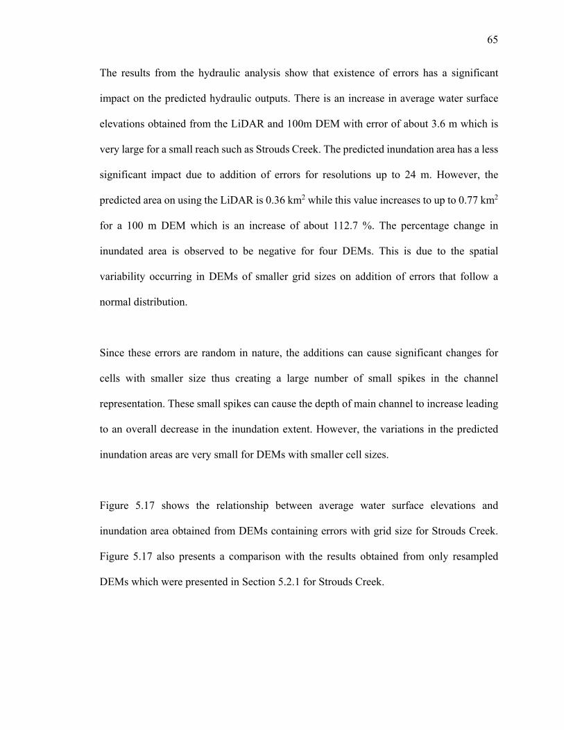
65

The results from the hydraulic analysis show that existence of errors has a significant

impact on the predicted hydraulic outputs. There is an increase in average water surface

elevations obtained from the LiDAR and 100m DEM with error of about 3.6 m which is

very large for a small reach such as Strouds Creek. The predicted inundation area has a less

significant impact due to addition of errors for resolutions up to 24 m. However, the

predicted area on using the LiDAR is 0.36 km2 while this value increases to up to 0.77 km2

for a 100 m DEM which is an increase of about 112.7 %. The percentage change in

inundated area is observed to be negative for four DEMs. This is due to the spatial

variability occurring in DEMs of smaller grid sizes on addition of errors that follow a

normal distribution.

Since these errors are random in nature, the additions can cause significant changes for

cells with smaller size thus creating a large number of small spikes in the channel

representation. These small spikes can cause the depth of main channel to increase leading

to an overall decrease in the inundation extent. However, the variations in the predicted

inundation areas are very small for DEMs with smaller cell sizes.

Figure 5.17 shows the relationship between average water surface elevations and

inundation area obtained from DEMs containing errors with grid size for Strouds Creek.

Figure 5.17 also presents a comparison with the results obtained from only resampled

DEMs which were presented in Section 5.2.1 for Strouds Creek.

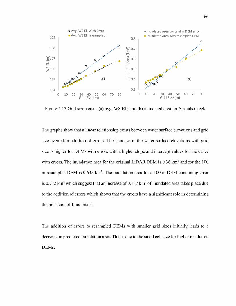
66

Figure 5.17 Grid size versus (a) avg. WS El.; and (b) inundated area for Strouds Creek

The graphs show that a linear relationship exists between water surface elevations and grid

size even after addition of errors. The increase in the water surface elevations with grid

size is higher for DEMs with errors with a higher slope and intercept values for the curve

with errors. The inundation area for the original LiDAR DEM is 0.36 km2 and for the 100

m resampled DEM is 0.635 km2. The inundation area for a 100 m DEM containing error

is 0.772 km2 which suggest that an increase of 0.137 km2 of inundated area takes place due

to the addition of errors which shows that the errors have a significant role in determining

the precision of flood maps.

The addition of errors to resampled DEMs with smaller grid sizes initially leads to a

decrease in predicted inundation area. This is due to the small cell size for higher resolution

DEMs.

164

165

166

167

168

169

0 10 20 30 40 50 60 70 80

WS El. (m)

Grid Size (m)

Avg. WS El. With Error

Avg. WS El. re‐sampled

0.3

0.4

0.5

0.6

0.7

0.8

0 10 20 30 40 50 60 70 80

Inundation Area (km

2)

Grid Size (m)

Inundated Area containing DEM error

Inundated Area with resampled DEM

a) b)

67

Even though the mean of the errors added to these DEMs is small, the small grid size

accounts to a larger spatial variability between the cells thus reducing the inundation extent.

But for larger grid sizes, the amount of error is very high and results in high estimation of

water surface elevations and inundation extents.

Figure 5.18 shows the cross-sections for station 6512.8 obtained from topographic datasets

of different resolution and magnitude of errors.

Figure 5.18 Cross-section station 6512.8 for (a) LiDAR; (b) 12 m DEM with error;

(c) 30 m DEM with error; and (d) 80 m DEM with error

180

185

190

195

200

0 200 400 600

Elevation (m)

Station (m)

LiDAR

179

184

189

194

199

0 200 400 600

Elevation (m)

Station (m)

12 m with error

180

185

190

195

200

0 200 400 600

Elevation (m)

Station (m)

30 m with error

180

184

188

192

196

0 200 400 600

Elevation (m)

Station (m)

80m with error

c) d)

b)a)

68

From Figure 5.18, it is evident that there is a significant loss in the river profile due to the

existence of DEM errors. The errors added to the original LiDAR DEM follow a normal

distribution, which can be seen from the fact that the 12 m, 30 m and 80 m DEMs have

substantial changes in the elevations across the entire cross-section. These spikes are the

main cause of increase in the flood inundation area. The cross-section obtained from the

100 m DEM completely misrepresents the main channel and the floodplain. This is due to

the existence of errors with a high magnitude and standard deviation throughout the entire

topography. Figure 5.19 shows a part of the flood maps for Strouds Creek developed from

DEMs with different magnitude of error and resolution.

Figure 5.19 Flood maps generated from (a) LiDAR; (b) 12 DEM with error;

(c) 30 m DEM with error; and (d) 80 m DEM with error

69

The flood maps show that addition of errors results in an increase in flood extents. The

original LiDAR DEM is inundated mostly around the main channel while the 100 m

resolution DEM with error predicts inundation for a larger area in the floodplain. The

magnitude of error added to the 100 m resolution DEM results in large variations in

elevations which show higher depth of inundation for some parts of the river channel while

no inundation for certain parts of the main channel itself.

5.4 Summary of Results

To analyze the effect of DEM resolution on hydraulic outputs, LiDAR data for five study

areas is resampled to coarser resolutions varying from 6 m to 100 m. The average water

surface elevations and inundation area for all the sites have a linear relationship with grid

size (R2 > 90 %). The variation in hydraulic outputs with DEM resolution is more

significant for study areas with urban land use. The impact of DEM resolution on hydraulic

outputs is more significant for smaller river reaches.

Resampling of higher resolution DEMs to coarser resolutions results in smoothing of

floodplain and decreases the accuracy of predicted hydraulic outputs. The presence of

artificial and natural levees reduces the impact of DEM resolution on inundation area

significantly as observed for East Fork White River. The impact of DEM resolution is also

influenced by the slope of the river channel and spatial variability in elevations which is

observed for Strouds Creek. The predicted flood extents for Brazos River do not increase

significantly because of the relatively flat terrain and large size of the study area.

70

In order to evaluate the relationship between DEM accuracy and hydraulic outputs, RMSE

values are calculated for three study areas. The results show that DEM error increases

linearly with grid size (R2 > 90 %). DEMs containing errors are generated for Strouds

Creek to analyze the effect of DEM error on hydraulic outputs. The hydraulic outputs are

highly influenced by the existence of errors. The predicted average water surface elevations

and inundation areas increase linearly with DEM errors. The flood maps generated using

the datasets containing errors have significant differences when compared to LiDAR

results.

These results explain the poor performance of coarser DEMs such as USGS NED 30 m

and SRTM when compared to LiDAR data. The hydraulic modeling results for these

datasets are affected by their coarse resolution and existence of DEM errors. Thus DEM

resolution and DEM errors are the main cause of differences in the accuracy of prediction

of hydraulic outputs. In order to improve the performance of coarser DEMs containing

errors, it is essential to use the relationships obtained in this study and apply them to these

topographic datasets. Chapter 6 discusses the application of the obtained relationships to

coarser DEMs with errors to improve the hydraulic modeling results for study areas where

LiDAR data are not available.

71

CHAPTER 6. DISCUSSIONS

6.1 Introduction

In order to understand the effect of two key attributes of a DEM (resolution and accuracy),

the concept of resampling and DEM error was used for hydraulic modeling. The results

from hydraulic analysis show that the water surface elevation and flood inundation area

have a linear relationship with grid size and DEM error. This relationship is well

established after analysis of five study areas with different reach lengths and land use types.

On plotting WS El. and inundation area versus grid size, high R2 values (greater than 90%)

are obtained for all study areas. This suggests that the coarser resolution DEMs over-

predict the water surface elevations and inundation area. This approach also suggests that

DEMs with larger grid sizes do not take into account the smaller depressions or elevations

that occur within a study area.

The second objective of this study is to use the linear relationship of DEM resolution and

accuracy with hydraulic outputs to improve the results of hydraulic modeling for areas

where LiDAR data is unavailable. These linear relationships were determined for LiDAR

data by resampling and introduction of errors. If these linear relationships hold true for

LiDAR generated DEMs, they can be applied to coarser resolution DEMs obtained from

other sources with lesser accuracy such as USGS NED 30 m and SRTM 90 m DEMs to

improve the hydraulic modeling results.

72

This chapter discusses the application of these relationships to other coarser DEMs. Since

the objective is to improve the hydraulic modeling results for these DEMs, the accuracy of

the analysis is defined relative to the original LiDAR DEMs for all the study areas. The

aim of this analysis is to get similar modeling results as LiDAR data from coarser DEMs

with more errors.

6.2 Development of New Analysis Approach

The quality of a DEM in predicting water surface elevations and flood inundation area can

be defined by its resolution and magnitude of errors (DEM accuracy). These hydraulic

outputs have been calculated for original LiDAR data with high resolution and accuracy

for all study areas. For this study, the objective is to obtain similar water surface elevations

and flood inundation area from coarser DEMs. The results obtained from DEM resampling

and error analysis from LiDAR data are analyzed and used to develop a new approach to

predict water surface elevations and flood extents using coarser DEMs. Using resampled

coarser resolution DEMs obtained from LiDAR data and the linear relationship, hydraulic

outputs are predicted for higher resolution DEMs. Similarly, the principle of linear

propagation of DEM errors with grid size is used to predict improved hydraulic outputs

from DEMs containing higher magnitude of errors.

Based on this principle, if water surface elevations obtained from only coarser resampled

DEMs (30 m-80 m resolution) are used to develop the linear relationship with grid size,

the R2 values obtained are still significantly high (greater than 90%).

73

The linear relationship obtained by WS El. of coarser resolutions DEMs is used to predict

the WS El. for higher resolution DEMs. This linear relationship with a positive slope

suggests that increasing grid size values over-predict the water surface elevations when

compared to the results obtained from high resolution LiDAR. An increasing slope also

suggests that the equation of the line obtained by using only higher grid size values can be

used to predict WS El. for smaller grid sizes. This relationship can be obtained for coarser

resolution DEMs containing errors and used to predict water surface elevations for higher

resolution DEMs containing less significant or no errors.

Thus, a new approach to predict hydraulic outputs for higher resolution datasets using the

results from coarser resolution datasets is developed. A similar approach is developed to

predict hydraulic outputs for higher accuracy datasets using lower accuracy datasets. This

approach is applied to coarser resolution DEMs obtained from LiDAR data resampling and

to DEMs containing errors also obtained from LiDAR data using the principle of normal

error distribution. Section 6.3 presents a detailed testing, analysis and application of the

new approach for LiDAR data. Once this approach is validated for LiDAR data, it is

applied to USGS NED 30 m and SRTM 90 m DEMs so that the hydraulic modeling results

obtained from these datasets can be improved relative to the LiDAR data.

6.3 Testing and Application of the New Approach

The analysis is carried out to check if results similar to LiDAR DEMs with high resolution

and accuracy can be obtained from coarser resolution and lesser accuracy DEMs. The

predicted results are compared to the original LiDAR DEMs which are the base scenarios.

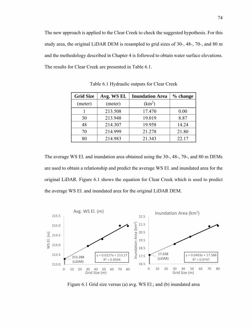
74

The new approach is applied to the Clear Creek to check the suggested hypothesis. For this

study area, the original LiDAR DEM is resampled to grid sizes of 30-, 48-, 70-, and 80 m

and the methodology described in Chapter 4 is followed to obtain water surface elevations.

The results for Clear Creek are presented in Table 6.1.

Table 6.1 Hydraulic outputs for Clear Creek

Grid Size Avg. WS El. Inundation Area % change

(meter) (meter) (km2)

1 213.508 17.470 0.00 30 213.948 19.019 8.87 48 214.307 19.958 14.24

70 214.999 21.278 21.80

80 214.983 21.343 22.17

The average WS El. and inundation area obtained using the 30-, 48-, 70-, and 80 m DEMs

are used to obtain a relationship and predict the average WS El. and inundated area for the

original LiDAR. Figure 6.1 shows the equation for Clear Creek which is used to predict

the average WS El. and inundated area for the original LiDAR DEM.

Figure 6.1 Grid size versus (a) avg. WS El.; and (b) inundated area

213.288(LiDAR)

y = 0.0227x + 213.27R² = 0.9594

213.0

213.5

214.0

214.5

215.0

215.5

0 10 20 30 40 50 60 70 80

WS El. (m)

Grid Size (m)

Avg. WS El. (m)

17.638(LiDAR)

y = 0.0493x + 17.588R² = 0.9747

16.5

17.5

18.5

19.5

20.5

21.5

22.5

0 10 20 30 40 50 60 70 80

Inundation Area (km

2)

Grid Size (m)

Inundation Area (km2)

75

The predicted average WS El. and inundation area are compared to the hydraulic outputs

obtained from the original LiDAR DEM for Clear Creek and the results are presented in

Table 6.2

Table 6.2 Comparison between observed and predicted results for Clear Creek

Data Grid Size LiDAR Predicted % error (meter) (base) (new approach) (<1%)

Avg. WS El. (m) 1 213.508 213.288 0.103

Inundation Area (km2) 1 17.470 17.638 -0.960

The results suggest that it is possible to apply the new approach to predict the average WS

El. and inundated area for original LiDAR DEMs using resampled coarser resolution

DEMs. The practical applicability of this approach is however less significant in predicting

flood maps if only the average WS El. and inundation areas are predicted.

6.3.1 Prediction of Water Surface Elevations

In order to predict better flood maps from coarser resolution DEMs, more accurate

prediction of WS El. across all cross-section stations is required and not just the average

water surface elevations. The results do suggest that decreasing the resolution of DEMs

results in over-prediction of hydraulic outputs and the effect of the errors that occur during

resampling can be minimized by using the suggested technique. This approach was further

tested for the entire cross-sections instead of comparing only the average WS El. for five

study areas.

76

To predict WS El. for every cross-section station, a linear regression model was developed

with river station and grid size as input parameters and water surface elevations as output.

Using linear regression, water surface elevations corresponding to original LiDAR DEM

grid size for every station across a reach were predicted using results obtained from coarser

resolution DEMs. However, using linear regression across an entire reach resulted in the

prediction of a linear water surface profile which is not true for most of the study areas. To

obtain the true water surface profile for a reach, the WS El. corresponding to resampled

30-, 48-, 60-, 70- and 80 m grid sizes for each cross-section station within a reach were

analyzed.

The results suggested that a linear relationship existed between WS El. and grid size for

most of the cross-section stations and not just the average WS El. for the entire reach with

only a few outliers. The slope and intercept of the line between WS El. and grid size

obtained from coarser resolution DEMs were calculated separately for each cross-section

station. These parameters were used to predict the WS El. for the original LiDAR DEM.

Table 6.3 illustrates the data and parameters used to obtain WS El. for 6 out of 86 cross-

section stations for Clear Creek.

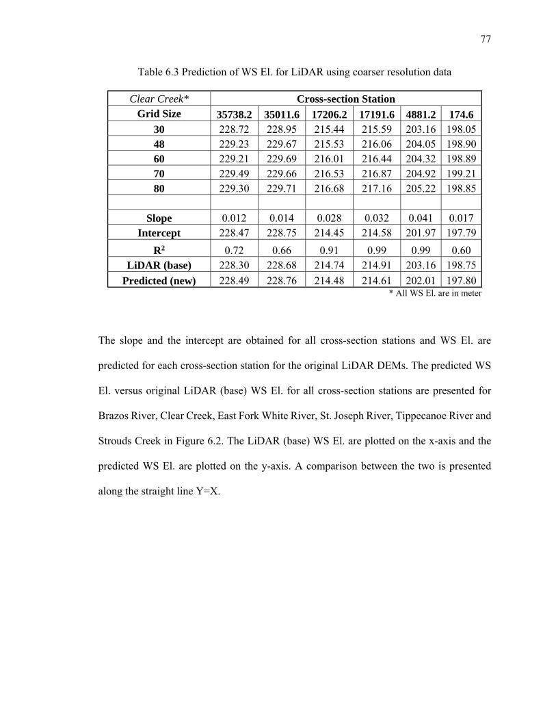
77

Table 6.3 Prediction of WS El. for LiDAR using coarser resolution data

Clear Creek* Cross-section Station Grid Size 35738.2 35011.6 17206.2 17191.6 4881.2 174.6

30 228.72 228.95 215.44 215.59 203.16 198.0548 229.23 229.67 215.53 216.06 204.05 198.9060 229.21 229.69 216.01 216.44 204.32 198.8970 229.49 229.66 216.53 216.87 204.92 199.2180 229.30 229.71 216.68 217.16 205.22 198.85

Slope 0.012 0.014 0.028 0.032 0.041 0.017 Intercept 228.47 228.75 214.45 214.58 201.97 197.79

R2 0.72 0.66 0.91 0.99 0.99 0.60 LiDAR (base) 228.30 228.68 214.74 214.91 203.16 198.75

Predicted (new) 228.49 228.76 214.48 214.61 202.01 197.80 * All WS El. are in meter

The slope and the intercept are obtained for all cross-section stations and WS El. are

predicted for each cross-section station for the original LiDAR DEMs. The predicted WS

El. versus original LiDAR (base) WS El. for all cross-section stations are presented for

Brazos River, Clear Creek, East Fork White River, St. Joseph River, Tippecanoe River and

Strouds Creek in Figure 6.2. The LiDAR (base) WS El. are plotted on the x-axis and the

predicted WS El. are plotted on the y-axis. A comparison between the two is presented

along the straight line Y=X.

78

Figure 6.2 Predicted WS El. versus original LiDAR (base) WS El. along the line Y=X

y = 0.9985xR² = 0.9994

16

18

20

22

24

26

28

30

16 18 20 22 24 26 28 30

Predicted W

S El. (m)

LiDAR WS El. (m)

Brazos River

y = 0.9993xR² = 0.9964

195

205

215

225

235

195 205 215 225 235

Predicted W

S El. (m)

LiDAR WS El. (m)

Clear Creek

y = 0.9995xR² = 0.9992

153

153.5

154

154.5

155

155.5

156

153 153.5 154 154.5 155 155.5 156

Predicted W

S El. (m)

LiDAR WS El. (m)

East Fork White River

y = 0.9985xR² = 0.907

219

220

221

222

223

224

219 220 221 222 223 224

Predicted W

S El. (m)

LiDAR WS El. (m)

St. Joseph River

y = 0.9996xR² = 0.8691

209

209.5

210

210.5

211

211.5

212

209 209.5 210 210.5 211 211.5 212

Predicted W

S El. (m)

LiDAR WS El. (m)

Tippecanoe River

y = 1.0004xR² = 0.9945

140

150

160

170

180

190

140 150 160 170 180 190

Predicted W

S El. (m)

LiDAR WS El. (m)

Strouds Creek

79

The graphs show that the predicted WS El. for Brazos River, Clear Creek, East Fork White

River and Strouds Creek match very well with the original LiDAR results. The

comparisons between predicted and LiDAR (base) WS El. for St. Joseph River show that

the predicted WS El. are under-predicted for some cross-section stations. The predicted

WS El. for Tippecanoe River for some cross-section stations do not match well with the

LiDAR results but the overall variation in the LiDAR and predicted data is not significant.

The results show that it is possible to use this approach to accurately predict water surface

elevations for original LiDAR datasets using hydraulic outputs generated from coarser

resolution datasets. This suggests that if this approach is applied to DEMs for regions where

LiDAR data is unavailable, the results of hydraulic modeling can be improved significantly.

For these regions, coarser resolution DEMs can be resampled to obtain the linear

relationship which can be used to predict water surface elevations. The results would be

improved estimates of water surface elevations as the values would be closer to the high

resolution LiDAR results.

To estimate the accuracy of the predicted data, RMSE of water surface elevations is

calculated using the LiDAR outputs as base values and the WS El. generated using

resampled coarser resolution datasets as predicted data. The RMSE values for each study

area are presented in Table 6.4.

80

Table 6.4 RMSE between observed and predicted WS El. for six study areas

Study Area Reach Length RMSE Datasets Used Avg. Slope (km) (m) (grid size in m)

Brazos River 59.9 0.08 30, 36, 48, 60, 80 0.00009 Clear Creek 39.0 0.66 30, 48, 60, 70, 80 0.00079

East Fork White River 20.2 0.10 30, 36, 48, 60 0.00001 St. Joseph River 11.1 0.55 30, 48, 70, 80 0.00018

Tippecanoe River 10.4 0.26 30, 36, 60, 70 0.00025

Strouds Creek 6.5 0.75 30, 48, 60, 80 0.00562

The RMSE values suggest this approach performs significantly well for Brazos River and

East Fork White River. Both these study areas are characterized by relatively flat terrain as

shown by the average slope values. The magnitude of the RMSE for all study areas is

directly affected by the variation in the WS El. across the entire reach and the reach length.

Strouds Creek being a small reach but with a high average slope has the highest RMSE

followed by Clear Creek. The overall results suggest that this approach predicts

significantly accurate water surface elevations when compared to LiDAR data for all cross-

section stations.

In order to check if a similar water surface profile is obtained from the predicted WS El.,

Figure 6.3 presents the water surface profiles for original LiDAR (base) WS El. and

predicted WS El. for Brazos River, Clear Creek and East Fork White River. The water

surface profile is presented relative to the minimum channel elevation (Min. Ch. El.).

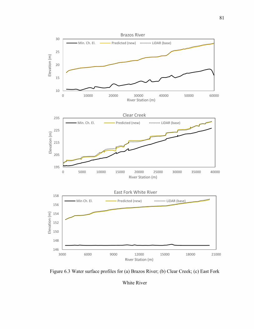
81

Figure 6.3 Water surface profiles for (a) Brazos River; (b) Clear Creek; (c) East Fork

White River

10

15

20

25

30

0 10000 20000 30000 40000 50000 60000

Elevation (m)

River Station (m)

Brazos River

Min. Ch. El. Predicted (new) LiDAR (base)

195

205

215

225

235

0 5000 10000 15000 20000 25000 30000 35000 40000

Elevation (m)

River Station (m)

Clear Creek

Min. Ch. El. Predicted (new) LiDAR (base)

146

148

150

152

154

156

158

3000 6000 9000 12000 15000 18000 21000

Elevation (m)

River Station (m)

East Fork White River

Min Ch. El. Predicted (new) LiDAR (base)

82

The difference between a high resolution LiDAR DEM and a DEM obtained from any

other data source such USGS NED 30 m and SRTM is the resolution of the dataset and the

amount of elevation error in measurements. If the effect of resolution and error on hydraulic

outputs is reduced, then the results obtained from these coarser DEMs can be significantly

improved. The application of the new approach on coarser DEMs has provided improved

estimates on hydraulic outputs and the impact of DEM resolution has been reduced.

The next step involves testing the applicability of this approach to improve the predicted

water surface elevations obtained from DEMs containing error. In order to test this, the

linear relationship technique was applied to DEMs containing random errors with a normal

distribution. These datasets were produced for Strouds Creek and slope and intercepts using

the relationship between WS El. and grid size were evaluated using 30-, 36-, 48-, 60- and

80 m resampled DEMs containing errors. For each cross-section station, slope and

intercepts were calculated using linear regression and predicted WS El. were compared to

the results from original LiDAR DEM.

Figure 6.4 shows the predicted WS El. using 30 m DEM containing errors and the predicted

WS El. using the new approach versus the results from the original LiDAR DEM. The

results from 30 m resampled DEM containing errors are shown to present the improvement

in the results obtained using the new approach.

83

Figure 6.4 Predicted versus LiDAR (base) WS El. for Strouds Creek along Y=X

The results show that this approach can be used to improve the predicted WS El. obtained

from coarser resolution topographic data containing errors. The RMSE (LiDAR base) of

WS El. using 30 m resampled DEM with error is reduced from 5.37 m to 0.68 m using the

new approach. Since these errors follow a normal distribution, there are certain cross-

sections stations which contain sudden depressions and changes in elevations. These cross-

section stations are removed from the regression equation to reduce the effect of outliers.

The WS El. generated using 30 m resampled DEM with error are clearly over-predicted

when compared to original LiDAR (base) results. Using the new approach, the predicted

WS El. are significantly closer to the LiDAR (base) results. Thus it can be concluded that

the new approach can be applied to coarser resolution DEMs containing errors to improve

the hydraulic modeling results.

140

145

150

155

160

165

170

175

180

185

140 145 150 155 160 165 170 175 180 185

Predicted W

S El. (m)

LiDAR WS El. (m)

y=x

Predicted

Original 30m

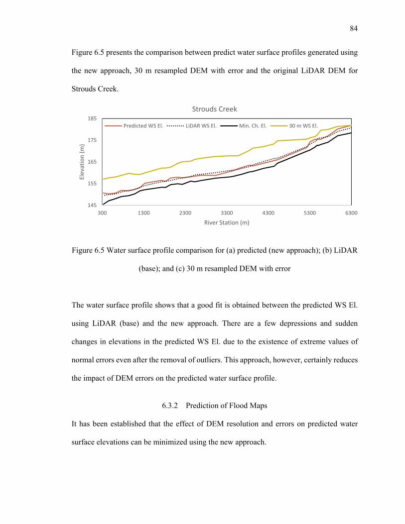
84

Figure 6.5 presents the comparison between predict water surface profiles generated using

the new approach, 30 m resampled DEM with error and the original LiDAR DEM for

Strouds Creek.

Figure 6.5 Water surface profile comparison for (a) predicted (new approach); (b) LiDAR

(base); and (c) 30 m resampled DEM with error

The water surface profile shows that a good fit is obtained between the predicted WS El.

using LiDAR (base) and the new approach. There are a few depressions and sudden

changes in elevations in the predicted WS El. due to the existence of extreme values of

normal errors even after the removal of outliers. This approach, however, certainly reduces

the impact of DEM errors on the predicted water surface profile.

6.3.2 Prediction of Flood Maps

It has been established that the effect of DEM resolution and errors on predicted water

surface elevations can be minimized using the new approach.

145

155

165

175

185

300 1300 2300 3300 4300 5300 6300

Elevation (m)

River Station (m)

Strouds Creek

Predicted WS El. LiDAR WS El. Min. Ch. El. 30 m WS El.

85

However, in order to predict more accurate flood maps relative to the LiDAR data from

coarser resolution topographic data containing errors, it is essential to apply the predicted

WS El. obtained using the new approach in developing flood maps. Since one of the

objectives of this study was to minimize the effect of errors on flood inundation maps,

further analysis was done by creating flood maps using ArcGIS from the predicted water

surface elevations. The predicted WS El. are exported to GIS and are used to generate a

TIN datasets which are converted into grid data using nearest neighbor interpolation

technique. The final step in creating flood maps involves subtracting the topographic

datasets from the generated water surface elevation DEM to obtain flood inundated area

(Merwade, 2012; Tate et al., 1999).

Water surface raster are generated for Tippecanoe River and Clear Creek by exporting the

WS El. calculated using the new approach into ArcGIS and flood maps are created by

subtracting the coarse resolution 30 m resampled DEMs from the generated water surface

raster. These flood maps are created solely from coarser resolution topographic datasets.

In order to compare the flood maps developed with the new approach with original LiDAR

generated maps, three quantitative indices are calculated: (1) inundation area; (2) % change

in inundation area; and (3) F-statistic (Bates & De Roo, 2000; Cook & Merwade, 2009;

Horritt & Bates, 2001). The F-statistic for Tippecanoe River and Clear Creek is calculated

using Equation 6.1.

100 ∗ Equation 6.1

86

Where Ao is the observed area of inundation (original LiDAR), Ap is the predicted area of

inundation (new approach) and Aop is the intersection of observed and predicted areas.

Table 6.5 presents the results of the comparison between flood maps created using

resampled 30 m DEM, new approach and original LiDAR DEM for Tippecanoe River and

Clear Creek.

Table 6.5 Comparisons of flood maps for Tippecanoe River and Clear Creek

LiDAR New Approach Resampled 30 m

Study Area (base) Area %

changeF-Stat Area

% change

F-Stat

(km2) (km2) (%) (km2) (%)

Tippecanoe River 2.94 2.80 -4.73 80.23 3.13 6.61 87.85

Clear Creek 17.47 16.64 -4.73 87.44 18.76 7.40 81.49

The results suggest that the flood inundation areas created using the new approach are

under-predicted (4.73 % less) for both Tippecanoe River and Clear Creek. The flood

inundation areas obtained using the 30 m resampled DEM are over-predicted and the

percentage change for the new approach is less for both areas. An F-statistic of 100 suggests

that there is complete match between the observed and predicted flood maps. For Clear

Creek, the F-statistic value improved from 81.49 % to 87.44 % when the new approach is

applied to the water surface elevations however, the F-statistic value reduces from 87.85 %

to 80.23 % for Tippecanoe River. This result highlights the importance of modeling DEM

errors present in the 30 m resampled dataset.

87

Since the final step to generate flood maps in ArcGIS requires the input of the original

topographic datasets, errors in these datasets can cause under-prediction of the inundated

areas. Even though the water surface elevations are predicted accurately when compared

to LiDAR results, the flood inundation maps can be improved only if the errors occurring

in the coarser resolution datasets are modeled and removed before subtracting the water

surface profile. If accuracy of the elevation data is improved, the resultant flood maps could

be more accurate when compared to the maps produced using the original LiDAR datasets.

6.4 Validation and Estimation for Different Topographic Datasets

The main objective of this study is to analyze the relationship of DEM resolution and

accuracy with hydraulic outputs. Studies in the past have concluded that high resolution

LiDAR data is the most accurate topographic data (Charlton et al., 2003; Gonga-

Saholiariliva et al., 2011; Hodgson et al., 2003; Smith et al., 2004). The application of

LiDAR generated DEMs in hydraulic modeling has suggested that these datasets are very

accurate in predicting water surface elevations and flood inundation maps (Casas et al.,

2006; Cook et al., 2009; Haile et al., 2005; Sanders, 2007; Schumann et al., 2008). However,

hydraulic modeling around the world is still largely carried out using other coarser

resolution and lower accuracy datasets because of the cost of acquisition and lack of

availability of LiDAR data.

In order to improve the accuracy of hydraulic results obtained from the widely used coarser

DEMs when compared to LiDAR results, relationships between hydraulic variables and

DEM attributes were developed in this study.

88

These relationships were obtained using resampling and error analysis of LiDAR data. The

application of these relationships to topographic datasets generated from other data sources

is discussed in this section.

The linear relationship between WS El. and grid size has been well established for

resampled DEMs created from LiDAR datasets. However, it is essential to check if the

other topographic datasets have the same relationship. USGS NED 30 m DEMs are one of

the most widely used topographic datasets in the United States being open source and easily

accessible. SRTM datasets are also widely used in the world even though, they are less

accurate than LiDAR and USGS DEMs. Section 6.3.1 presents the analysis and application

of the new approach for USGS 30 m NED DEMs while Section 6.3.2 presents the analysis

and application for SRTM 90 m resolution DEMs.

6.4.1 USGS NED 30 m Resolution DEMs

In order to establish the relationship between WS El. and DEM resolution for USGS DEMs,

study areas on Strouds Creek, Tippecanoe River, St. Joseph River and East Fork White

River were used. NED 30 m DEMs were resampled into DEMs of larger grid sizes and

average water surface elevations were calculated using HEC-RAS. Figure 6.6 shows the

relationship of USGS DEMs with grid size and presents a comparison between USGS

DEMs and LiDAR datasets for four study areas.

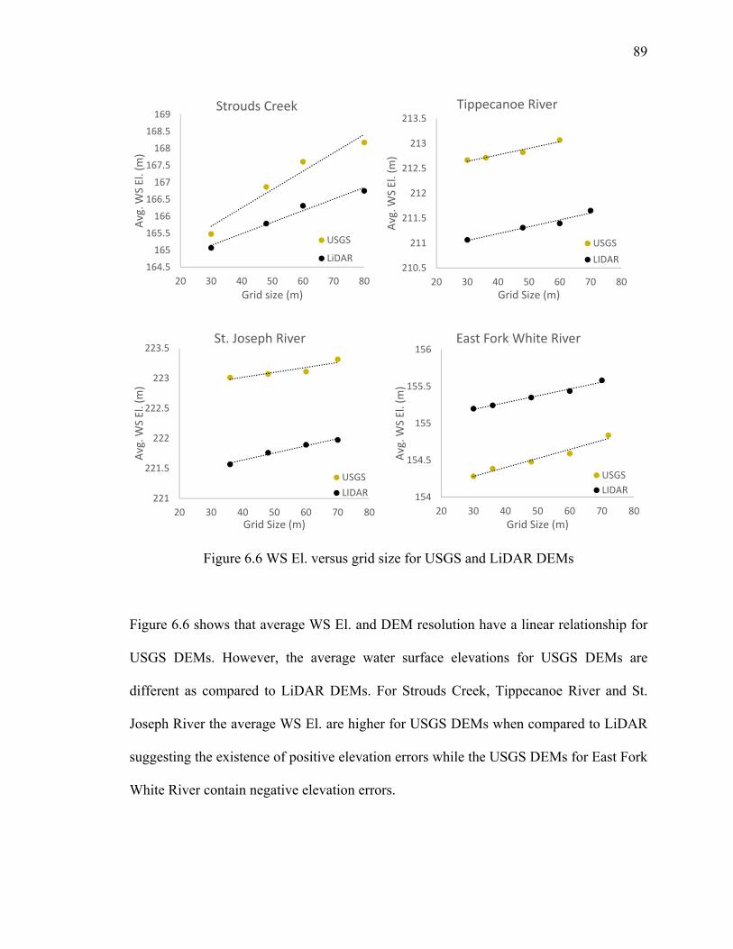
89

Figure 6.6 WS El. versus grid size for USGS and LiDAR DEMs

Figure 6.6 shows that average WS El. and DEM resolution have a linear relationship for

USGS DEMs. However, the average water surface elevations for USGS DEMs are

different as compared to LiDAR DEMs. For Strouds Creek, Tippecanoe River and St.

Joseph River the average WS El. are higher for USGS DEMs when compared to LiDAR

suggesting the existence of positive elevation errors while the USGS DEMs for East Fork

White River contain negative elevation errors.

164.5

165

165.5

166

166.5

167

167.5

168

168.5

169

20 30 40 50 60 70 80

Avg. W

S El. (m)

Grid size (m)

Strouds Creek

USGS

LiDAR210.5

211

211.5

212

212.5

213

213.5

20 30 40 50 60 70 80

Avg. W

S El. (m)

Grid Size (m)

Tippecanoe River

USGS

LIDAR

221

221.5

222

222.5

223

223.5

20 30 40 50 60 70 80

Avg. W

S El. (m)

Grid Size (m)

St. Joseph River

USGS

LIDAR 154

154.5

155

155.5

156

20 30 40 50 60 70 80

Avg. W

S El. (m)

Grid Size (m)

East Fork White River

USGS

LIDAR

90

The existence of these errors is the main cause of over-prediction or under-prediction in

water surface elevations and inundation areas for USGS DEMs when compared to LiDAR

generated hydraulic outputs. After establishing the linear relationship for USGS DEMs,

Strouds Creek and East Fork White River study areas are chosen for analysis to reduce the

impact of DEM errors using the new approach presented in Section 6.2.

The USGS NED 30 m DEMs are coarse resolution topographic datasets containing

elevation errors when compared to the LiDAR DEMs. The analysis for resampled DEMs

containing errors was carried out for Strouds Creek and the results were presented in

Section 5.3. It was observed that RMSE has a linear relationship with grid size. Using this

relationship, RMSE values for larger grid sizes can be predicted if the RMSE values for

smaller grid sizes are known. The RMSE for USGS 30 m DEMs was calculated using

LiDAR datasets as base values for Strouds Creek and East Fork White River. Using this

value and the linear relationship between RMSE and grid size, RMSE values for coarser

resampled USGS DEMs are predicted. The increase in WS El. for coarser resolution DEMs

was attributed as an effect of resampling and existence of elevation errors in Section 5.3.

The hypothesis is that if the 30 m USGS DEM contains an error of known RMSE value, a

DEM of grid size larger than 30 m would contain an RMSE equal to the predicted RMSE

using the linear relationship. The results in Section 5.3 show that the effect of these errors

can be reduced by predicting WS El. using the new approach which involves developing a

relationship between predicted WS El. of resampled DEMs containing errors and grid size.

91

The predicted RMSE values obtained using the linear relationship are used to create error

raster with grid sizes 36-, 48-, 60- and 80 m. These error rasters are added to the resampled

USGS DEMs with grid sizes greater than 30 m to obtain new topographic datasets with

containing errors. The error raster are created using the normal distribution approximation.

After adding these errors, the new topographic datasets are used to create geometry files

using HEC-GeoRAS which are exported into HEC-RAS to obtain water surface elevations.

These datasets now have similar attributes to the DEMs created for Strouds Creek

containing errors in Section 4.3.

The modeled WS El. from these datasets are used to predict water surface elevations for

all cross-section stations using the approach described in Section 6.1. These water surface

elevations are then compared with the original LiDAR generated results.

Figure 6.7 presents a comparison of the predicted WS El. using the new approach and the

original USGS DEMs with the original LiDAR (base) DEMs for East Fork White River

and Strouds Creek.

92

Figure 6.7 LiDAR (base) versus predicted WS El. for (a) East Fork White River and (b)

Strouds Creek

Figure 6.7 shows a comparison along the line Y=X where Y corresponds to the predicted

WS El. obtained from the new approach and original USGS DEM while X corresponds to

the WS El. obtained from the original LiDAR. The results show that the impact of errors

on WS El. is reduced significanlty for East Fork White River using the new approach and

the predicted WS El. are more closer to the original LiDAR values when compared to the

USGS 30 m DEM. For Srouds Creek, there is less significant increase in the accuracy of

predicted WS El., however, this is also due to the small magnitude of errors in the 30 m

USGS DEM for Strouds Creek. To quantify and compare the performance of the predicted

WS El. and USGS WS El. with the LiDAR results, RMSE of WS El. is calculated using

all cross-section stations as observed points. Table 6.6 presents the RMSE in WS El. for

East Fork White River and Strouds Creek.

149

151

153

155

157

159

149 151 153 155 157 159

Predicted W

S El. (m)

LiDAR WS El. (m)

Y=X Predicted USGS Original USGS

143

153

163

173

183

193

143 153 163 173 183 193

Predicted W

S El. (m)

LiDAR WS El. (m)

Y=X Predicted USGS Original USGS

a) b)

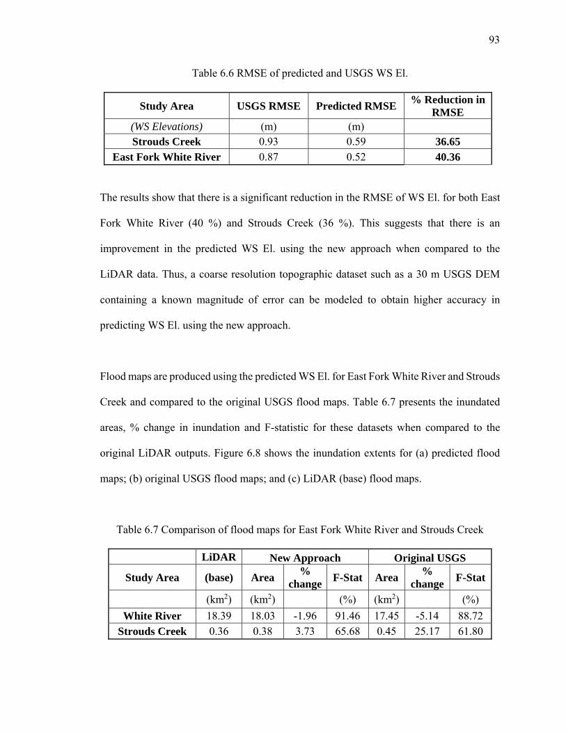
93

Table 6.6 RMSE of predicted and USGS WS El.

Study Area USGS RMSE Predicted RMSE % Reduction in

RMSE (WS Elevations) (m) (m) Strouds Creek 0.93 0.59 36.65

East Fork White River 0.87 0.52 40.36

The results show that there is a significant reduction in the RMSE of WS El. for both East

Fork White River (40 %) and Strouds Creek (36 %). This suggests that there is an

improvement in the predicted WS El. using the new approach when compared to the

LiDAR data. Thus, a coarse resolution topographic dataset such as a 30 m USGS DEM

containing a known magnitude of error can be modeled to obtain higher accuracy in

predicting WS El. using the new approach.

Flood maps are produced using the predicted WS El. for East Fork White River and Strouds

Creek and compared to the original USGS flood maps. Table 6.7 presents the inundated

areas, % change in inundation and F-statistic for these datasets when compared to the

original LiDAR outputs. Figure 6.8 shows the inundation extents for (a) predicted flood

maps; (b) original USGS flood maps; and (c) LiDAR (base) flood maps.

Table 6.7 Comparison of flood maps for East Fork White River and Strouds Creek

LiDAR New Approach Original USGS

Study Area (base) Area %

changeF-Stat Area

% change

F-Stat

(km2) (km2) (%) (km2) (%)

White River 18.39 18.03 -1.96 91.46 17.45 -5.14 88.72

Strouds Creek 0.36 0.38 3.73 65.68 0.45 25.17 61.80

94

Figure 6.8 Inundation extents for East Fork White River and Strouds Creek

The results for East Fork White River show that both the predicted flood maps obtained

using the new approach and the original USGS DEM under-predict the inundation area.

However, the percentage change in inundation area is reduced from 5.14 % for USGS DEM

to 1.96 % for the new predicted flood map. The F-statistic comparison also shows an

improvement in the intersected areas for the predicted flood map (91.46 %) when compared

to the original USGS flood map (88.72 %). For Strouds Creek, both the predicted flood

map and the original USGS flood map over-predict the inundation area. The percentage

change in inundation area is reduced from 25.1 % for USGS DEM to 3.7 % for the new

predicted flood map. The F-statistic comparison for Strouds Creek shows an improvement

in the intersected areas for the predicted flood map (65.6 %) when compared to the original

USGS flood map (61.8 %).

95

A part of the flood map for East Fork White River is shown in Figure 6.8 which highlights

the improvement in the predicted inundated areas. Both the predicted and USGS DEM

under-predict the flood extents, however, the predicted flood map using the new approach

gives a more accurate representation of inundated areas for regions where the UGSS DEM

shows no inundation and the LiDAR DEM shows inundation. For Strouds Creek, both the

predicted and USGS DEM over-predict the inundation extents, however, the predicted

flood map gives a more accurate representation of inundated areas for regions where the

USGS DEM shows inundation and the LiDAR DEM shows no inundation. These results

show that it is possible to reduce the impact of DEM resolution and DEM errors on WS El.

and flood extents for USGS DEMs using the new approach.

6.4.2 SRTM 90 m Resolution DEMs

SRTM DEMs contain a significant amount of errors when compared to LiDAR DEMs and

do not predict the hydraulic outputs accurately. However, LiDAR datasets are not available

globally which justifies the importance of improving the accuracy of SRTM DEMs in

predicting flood maps. In order to evaluate the performance of the new approach on SRTM

DEMs, Brazos River, the largest study area and Strouds Creek, the smallest study area are

chosen for analysis. The RMSE for these DEMs is calculated using the LiDAR data points

as base values. After calculating the RMSE, the linear relationship of RMSE with grid size

is used to create resampled datasets containing errors. These datasets are used to check the

relationship between WS El. and grid size which is shown in Figure 6.9.

96

Figure 6.9 WS El. of SRTM DEMs versus grid size for (a) Strouds Creek and (b) Brazos

River

After confirming that a linear relationship exists between WS El. and grid size, the results

are used to predict WS El. for each cross-section station using the new approach. The

original SRTM DEMs for Brazos River and Strouds Creek have positive elevation errors

and highly over-predict the WS El. and flood extents. After applying the new approach to

model these errors, the original SRTM WS El. and predicted WS El. are compared to the

LiDAR outputs as shown in Figure 6.10.

y = 0.0667x + 167.34R² = 0.9565

167

168

169

170

171

172

173

0 20 40 60 80

Avg. W

S El. (m)

Grid Size (m)

Strouds Creek‐ SRTM

y = 0.0551x + 20.876R² = 0.9996

20.5

21

21.5

22

22.5

23

23.5

24

24.5

25

25.5

0 20 40 60 80

Avg. W

S El. (m)

Grid Size (m)

Brazos River‐SRTM

a) b)

97

Figure 6.10 LiDAR (base) versus predicted WS El. for (a) Strouds Creek and (b) Brazos

River

The comparisons show that the original SRTM WS El. are highly inaccurate and over-

estimated however the predicted WS El. using the new approach are comparatively more

accurate and closer to the base LiDAR WS El.

Table 6.8 shows the comparison in the RMSE of WS El. for Brazos River and Strouds

Creek.

145

155

165

175

185

145 155 165 175 185Predicted W

S El. (m)

LiDAR WS El. (m)

Y=X Predicted SRTM original srtm

15

17

19

21

23

25

27

29

31

15 17 19 21 23 25 27 29 31

Predicted W

S El. (m)

LiDAR WS El. (m)

y=x Predicted SRTM Original SRTM

b)

a)

98

Table 6.8 RMSE of SRTM and predicted WS El.

Study Area SRTM RMSE Predicted RMSE % Reduction in

RMSE (m) (m)

Brazos River 2.72 1.33 51.05

Strouds Creek 8.77 3.06 65.14

The results show a significant improvement in the RMSE of WS El. for both Brazos River

(51.05 %) and Strouds Creek (65.14 %). This suggests that the impact of DEM errors on

WS El. has been substantially reduced using the new approach. The predicted WS El. are

used to generate flood maps and are compared with the original SRTM generated flood

map. Table 6.9 presents the comparison between inundation area, % change in inundation

and F-statistic for Brazos River and Strouds Creek.

Table 6.9 Comparison of flood maps for Brazos River and Strouds Creek

Observed New Approach Original SRTM

Study Area LiDAR Area %

changeF-Stat Area

% change

F-Stat

(km2) (km2) (%) (km2) (%)

Brazos River 150.07 117.95 -21.41 59.75 99.08 -33.98 56.86

Strouds Creek 0.36 0.98 168.97 15.41 1.25 245.03 15.98

The results show that both the predicted flood map and SRTM flood map do not perform

well in predicting the inundation extents for Brazos River with F-statistic values of 59.75 %

for predicted flood map and 56.86 % for original SRTM flood map. However, the original

SRTM flood map under-predicts the inundation area by 33.98 % while the predicted flood

map under-predicts the inundation area by 21.41 % when compared to LiDAR data.

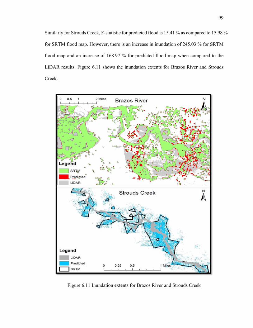
99

Similarly for Strouds Creek, F-statistic for predicted flood is 15.41 % as compared to 15.98 %

for SRTM flood map. However, there is an increase in inundation of 245.03 % for SRTM

flood map and an increase of 168.97 % for predicted flood map when compared to the

LiDAR results. Figure 6.11 shows the inundation extents for Brazos River and Strouds

Creek.

Figure 6.11 Inundation extents for Brazos River and Strouds Creek

100

The predicted inundation extents for Brazos River show a 33.98 % under-prediction of

inundation area by the original SRTM flood map while the predicted flood map using the

new approach reduces the under-prediction of the inundation area when compared to

LiDAR results. It is evident from the F-statistic that even though there is an under-

prediction in inundation area, the extent of inundation is better attributed by the new

approach. Both the original SRTM and new approach perform poorly in estimating the

inundation extents for Strouds Creek.

However, from these results it can be inferred that the WS El. predicted using the new

approach are more accurate than the original SRTM DEM. The flood maps for both the

study areas are inaccurately represented because of the spatial distribution of errors added

to the topographic datasets. In order to predict the inundation extents more accurately, the

distribution of errors has to be modeled correctly. For a small study area such as Strouds

Creek, a highly variable error distribution is difficult to be removed using the normal

distribution assumption. The predicted flood map for Strouds Creek consists of random

depressions and elevations that are caused due to removal of errors with a normal

approximations. For points in a flat terrain, these depressions cause the water depth to

become greater than zero and these areas are predicted as inundated.

It is essential to understand the spatial distribution of DEM errors in order to predict flood

maps more accurately for smaller reaches such as Strouds Creek. The impact of these

depressions is less significant for Brazos River because of the size of the study area.

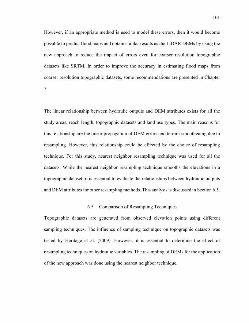
101

However, if an appropriate method is used to model these errors, then it would become

possible to predict flood maps and obtain similar results as the LiDAR DEMs by using the

new approach to reduce the impact of errors even for coarser resolution topographic

datasets like SRTM. In order to improve the accuracy in estimating flood maps from

coarser resolution topographic datasets, some recommendations are presented in Chapter

7.

The linear relationship between hydraulic outputs and DEM attributes exists for all the

study areas, reach length, topographic datasets and land use types. The main reasons for

this relationship are the linear propagation of DEM errors and terrain-smoothening due to

resampling. However, this relationship could be effected by the choice of resampling

technique. For this study, nearest neighbor resampling technique was used for all the

datasets. While the nearest neighbor resampling technique smooths the elevations in a

topographic dataset, it is essential to evaluate the relationships between hydraulic outputs

and DEM attributes for other resampling methods. This analysis is discussed in Section 6.5.

6.5 Comparison of Resampling Techniques

Topographic datasets are generated from observed elevation points using different

sampling techniques. The influence of sampling technique on topographic datasets was

tested by Heritage et al. (2009). However, it is essential to determine the effect of

resampling techniques on hydraulic variables. The resampling of DEMs for the application

of the new approach was done using the nearest neighbor technique.

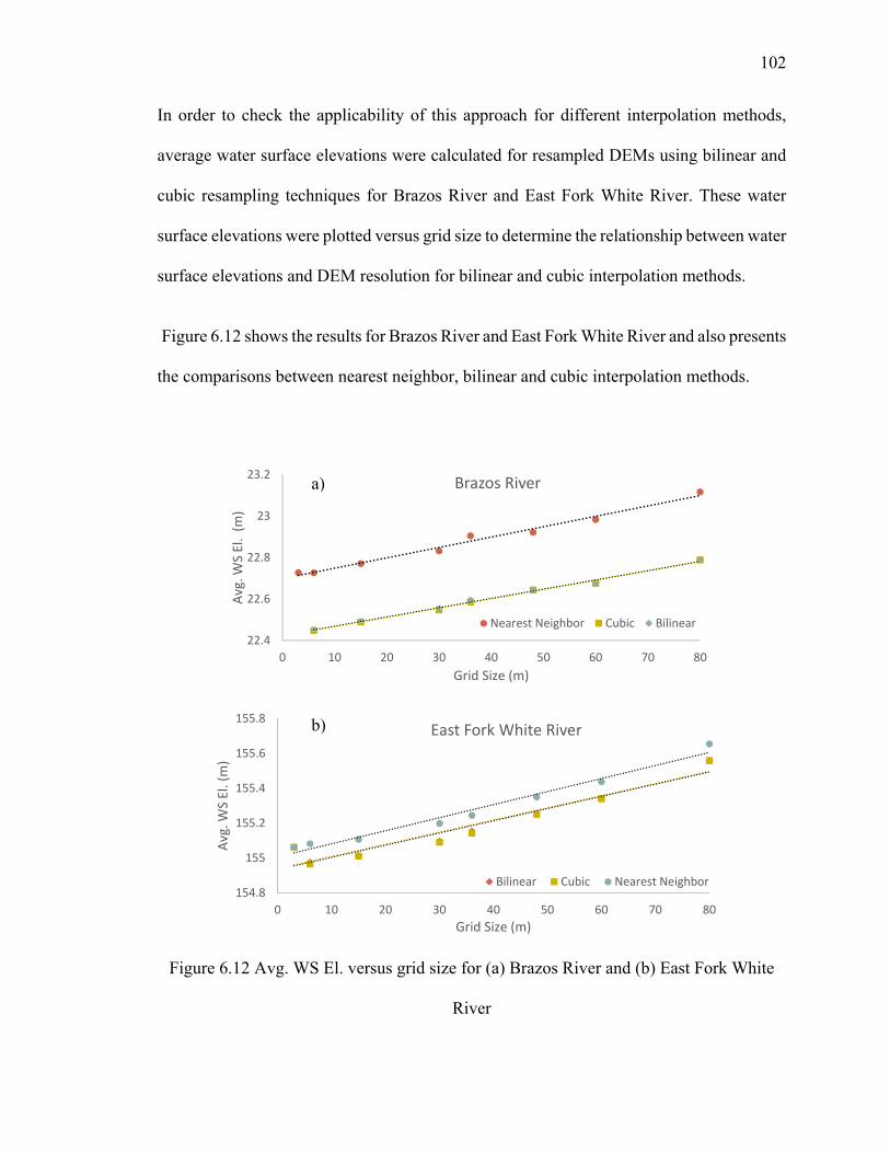
102

In order to check the applicability of this approach for different interpolation methods,

average water surface elevations were calculated for resampled DEMs using bilinear and

cubic resampling techniques for Brazos River and East Fork White River. These water

surface elevations were plotted versus grid size to determine the relationship between water

surface elevations and DEM resolution for bilinear and cubic interpolation methods.

Figure 6.12 shows the results for Brazos River and East Fork White River and also presents

the comparisons between nearest neighbor, bilinear and cubic interpolation methods.

Figure 6.12 Avg. WS El. versus grid size for (a) Brazos River and (b) East Fork White

River

22.4

22.6

22.8

23

23.2

0 10 20 30 40 50 60 70 80

Avg. W

S El.  (m

)

Grid Size (m)

Brazos River

Nearest Neighbor Cubic Bilinear

154.8

155

155.2

155.4

155.6

155.8

0 10 20 30 40 50 60 70 80

Avg. W

S El. (m)

Grid Size (m)

East Fork White River

Bilinear Cubic Nearest Neighbor

a)

b)

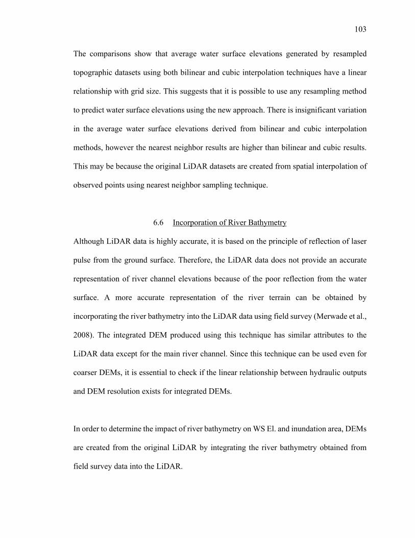
103

The comparisons show that average water surface elevations generated by resampled

topographic datasets using both bilinear and cubic interpolation techniques have a linear

relationship with grid size. This suggests that it is possible to use any resampling method

to predict water surface elevations using the new approach. There is insignificant variation

in the average water surface elevations derived from bilinear and cubic interpolation

methods, however the nearest neighbor results are higher than bilinear and cubic results.

This may be because the original LiDAR datasets are created from spatial interpolation of

observed points using nearest neighbor sampling technique.

6.6 Incorporation of River Bathymetry

Although LiDAR data is highly accurate, it is based on the principle of reflection of laser

pulse from the ground surface. Therefore, the LiDAR data does not provide an accurate

representation of river channel elevations because of the poor reflection from the water

surface. A more accurate representation of the river terrain can be obtained by

incorporating the river bathymetry into the LiDAR data using field survey (Merwade et al.,

2008). The integrated DEM produced using this technique has similar attributes to the

LiDAR data except for the main river channel. Since this technique can be used even for

coarser DEMs, it is essential to check if the linear relationship between hydraulic outputs

and DEM resolution exists for integrated DEMs.

In order to determine the impact of river bathymetry on WS El. and inundation area, DEMs

are created from the original LiDAR by integrating the river bathymetry obtained from

field survey data into the LiDAR.

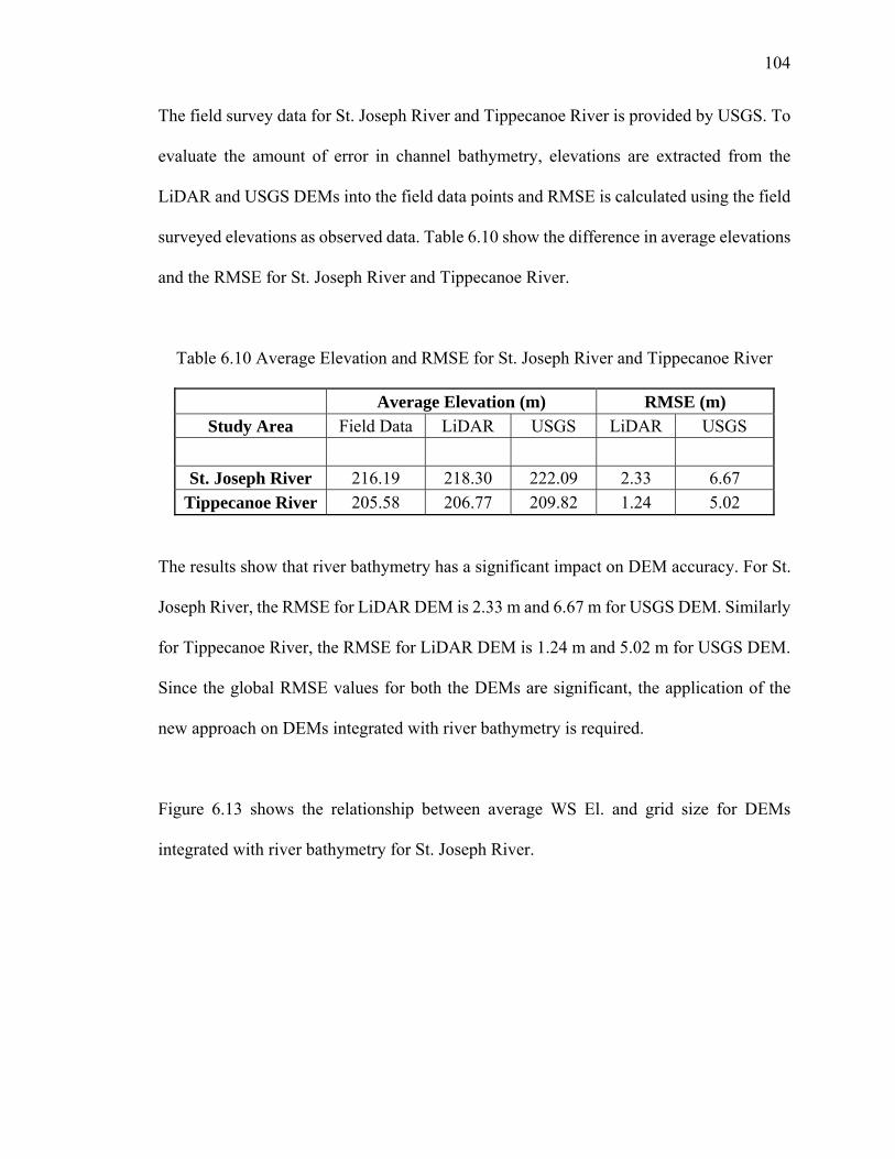
104

The field survey data for St. Joseph River and Tippecanoe River is provided by USGS. To

evaluate the amount of error in channel bathymetry, elevations are extracted from the

LiDAR and USGS DEMs into the field data points and RMSE is calculated using the field

surveyed elevations as observed data. Table 6.10 show the difference in average elevations

and the RMSE for St. Joseph River and Tippecanoe River.

Table 6.10 Average Elevation and RMSE for St. Joseph River and Tippecanoe River

Average Elevation (m) RMSE (m)

Study Area Field Data LiDAR USGS LiDAR USGS

St. Joseph River 216.19 218.30 222.09 2.33 6.67

Tippecanoe River 205.58 206.77 209.82 1.24 5.02

The results show that river bathymetry has a significant impact on DEM accuracy. For St.

Joseph River, the RMSE for LiDAR DEM is 2.33 m and 6.67 m for USGS DEM. Similarly

for Tippecanoe River, the RMSE for LiDAR DEM is 1.24 m and 5.02 m for USGS DEM.

Since the global RMSE values for both the DEMs are significant, the application of the

new approach on DEMs integrated with river bathymetry is required.

Figure 6.13 shows the relationship between average WS El. and grid size for DEMs

integrated with river bathymetry for St. Joseph River.

105

Figure 6.13 Avg. WS El. versus grid size for Bathymetry LiDAR for St. Joseph River

Figure 6.13 shows that the linear relationship between WS El. and grid size exists even for

integrated DEMs. This suggests that the impact of errors on WS El. and inundation area

can be reduced significantly for coarse resolution topographic data by incorporating the

river channel bathymetry and using the new approach to model WS El.

Table 6.11 shows the comparison between flood maps generated from LiDAR DEM with

and without river bathymetry for St. Joseph River and Tippecanoe River.

Table 6.11 Comparison of flood maps for St. Joseph River and Tippecanoe River

Study Area Bathymetry_LiDAR LiDAR % change F-Statistic

(km2) (km2)    (%)

St. Joseph River 2.16 3.16 46.22 67.76

Tippecanoe River 2.94 3.58 21.80 80.08

y = 0.019x + 219.28R² = 0.9792

219.2

219.4

219.6

219.8

220

220.2

220.4

220.6

220.8

221

0 10 20 30 40 50 60 70 80

Avg. W

S El. (m)

Grid Size (m)

St. Joseph Bathymetry

106

There is a significant reduction in inundated area after incorporating channel bathymetry

into the LiDAR DEMs with a 46.2 % change for St. Joseph River and 21.8 % change for

Tippecanoe River. Figure 6.14 illustrates this change by comparing the inundation extents

for LiDAR DEMs with and without river bathymetry.

Figure 6.14 Inundation Extents for (a) St. Joseph River and (b) Tippecanoe River

107

CHAPTER 7. SUMMARY AND CONCLUSIONS

7.1 Effect of DEM Resolution on Hydraulic Outputs

The first objective of this study was to establish a relationship between hydraulic outputs

and DEM resolution. This is accomplished using LiDAR DEMs for five study areas by

resampling LiDAR DEMs into different grid sizes and obtaining water surface elevations

and flood inundation areas using ArcGIS and HEC-RAS. For a given flow and boundary

conditions, the average water surface elevations and grid size have a linear relationship

with a positive slope which is illustrated by high R2 (>90%) for all study areas. This

suggests that water surface elevations for all cross-section stations increase with decreasing

DEM resolution. This may be due to the smoothening effect on topography, high slope

gradients and loss of information about depressions. The change in water surface elevations

is less significant up to 20 m resolution but increases significantly for larger grid sizes.

The predicted flood inundation areas for all the sites increase with decreasing DEM

resolution. This suggests that DEMs of coarser resolution over-predict the flood extents.

The total inundation area and grid size also have a linear relationship with a positive slope.

The difference in predicted inundation area between the original LiDAR and 100 m

resolution DEM is largest for Strouds Creek (74.8 %) and smallest for East Fork White

River (3.18 %).

107

The quality of flood maps also decreases with increasing grid size for all study areas. These

results highlight the importance of DEM resolution in flood mapping especially for smaller

river reaches and river reaches with high slope gradients.

7.2 Effect of DEM Error on Hydraulic Outputs

This topic addresses the impact of elevation errors on water surface elevations and

inundation areas. A comparison of RMSE with grid size shows that the amount of error

increases with decreasing DEM resolution. The RMSE versus grid size comparisons for

three sites suggests a linear relationship with high R2 (> 90%). The water surface elevations

and inundation areas have a linear relationship with DEMs of different resolutions and

magnitude of errors. This relationship suggests that a coarse resolution DEM contains more

errors in elevations as compared to higher resolution LiDAR DEMs.

The existence of these errors results in over-prediction of both water surface elevations and

inundation areas for Strouds Creek. The average water surface elevations are over-

predicted about 3.65 m and inundation areas about 112.7 % for a DEM containing errors

of grid size 80 m when compared to the original LiDAR results. The errors that were added

to these DEMs were based on the assumption of normal distribution. Since a lot of studies

have focused on modeling the spatial distribution of DEM errors but no certain

relationships have been established, the third objective of this study aims to reduce the

impact of these errors on hydraulic outputs and not try to model the errors.

109

7.3 Development of a New Approach to Reduce the Impact of Errors

Both DEM resolution and DEM errors have a significant impact on hydraulic outputs. In

order to reduce this impact and to predict more accurate water surface elevations and flood

maps, the relationship of these attributes with grid size and errors developed in this study

is used. It is assumed that if the smallest grid size DEM (cell size approaching zero) is used

to predict flood maps, the results would be highly accurate. It is speculated that since the

water surface elevations increase with grid size and the small grid size DEMs predict

hydraulic outputs with higher precision, the water surface elevations obtained using the

larger grid sizes can be used to predict water surface elevations for smaller grid sizes.

To validate this hypothesis, the coarse resolution DEMs are used to develop the linear

relationship between water surface elevations and grid size for Clear Creek. This

relationship is used to model water surface elevations for all cross-section sections for a

higher resolution DEM. These modeled results are compared to the outputs generated using

high resolution LiDAR DEMs for all six study areas. The results show that the predicted

water surface elevations are very accurate relative to LiDAR results which can be seen by

the low RMSEs for all the sites. These water surface elevations are then used to predict

flood maps. The effect of DEM errors on water surface elevations is also reduced using

this approach. Instead of using only resampled DEMs to develop the linear relationship,

resampled DEMs containing errors are used. The results for Strouds Creek show that

significantly improved estimates of water surface elevations are produced using coarse

resolution topographic data containing errors.

110

To further evaluate the applicability of this approach for predicting better flood maps from

coarse resolution datasets, USGS 30 m DEMs and SRTM 90 m resolution DEMs are used.

The application of the new approach to both these datasets shows a significant

improvement in accuracy of water surface elevations when compared to LiDAR DEMs.

There is a reduction of 36.6 % in the RMSE of water surface elevations for USGS DEMs

modified using the new approach for Strouds Creek and a 40.3 % reduction in RMSE for

East Fork White River. The flood maps generated using these water surface elevations also

perform significantly better than the original USGS DEMs.

The accuracy of water surface elevations for coarse resolution SRTM DEMs is also

increased significantly for Strouds Creek with a reduction of 65 % in the RMSE and 51 %

for Brazos River. Since the SRTM DEMs contain large amount of elevation errors, the

normal distribution assumption of errors does not produce significantly better results in

predicting flood maps.

To check if the linear relationship between water surface elevations and grid size exists for

DEMs which are not resampled using nearest neighbor technique, both bilinear and cubic

interpolation methods are applied to the DEMs. The results show that for grid size up to

100 m resolution, the linear relationship is not affected by the interpolation technique.

Incorporating river bathymetry into the DEMs increases the accuracy of flood maps (Cook

et al., 2009). However, to check if the new approach is applicable to DEMs that are

integrated with river bathymetry, a further study is carried out.

111

The linear relationship between water surface elevations and grid size is still valid for

DEMs integrated with river bathymetry. Thus it is established that this approach can be

used to model water surface elevations for DEMs obtained from any source, sampling

technique, resolution (up to 100 m established for this study) and magnitude of errors.

7.4 Future Work and Recommendations

From this study, it can be established that the new approach can be applied to coarse

resolution topographic data to improve the predicted water surface elevations and flood

inundation areas. Since LiDAR data is not available for the entire United States, coarser

resolution topographic datasets which are available easily can be used with the new

approach to significantly improve the hydraulic modeling results obtained from these

datasets. The expected water surface elevations and inundation areas for any area can be

known using the relationships obtained in this study. However, in order to predict the

inundation extents with precision, further analysis is required on the removal of errors from

the DEMs. Even a high resolution dataset such as a LiDAR does not contain an accurate

representation of the main channel bathymetry.

Future work on hydraulic modeling and flood inundation mapping should consider the

optimum representation of the spatial characteristics of DEM errors. Even if it is possible

to predict water surface elevations more accurately using the new approach, without an

accurate spatial representation of DEM errors, it is difficult to obtain more accuracy in

predicting flood extents.

112

Further studies may look into the application of the rating relationships developed between

vertical elevation errors and spatial variability by Heritage et al. (2009).

For this study, there was no change in the boundary conditions, calibration parameters,

Manning’s n. This was done to account for the changes in water surface elevations only

due to topography. The analysis of the results of this study can be used to develop

guidelines for flood mapping. For small study areas with urban land use, the USGS 30 m

DEMs represent the terrain fairly accurately. For such study areas, if the river bathymetry

is integrated into a USGS DEM and the approach developed in this study is used to predict

water surface elevations, the resulting flood maps would be highly accurate as compared

to the original USGS DEMs. Thus the cost of acquisition of LiDAR DEMs for such study

areas can be saved.

For large study areas with a relatively deep main river channel, most of the flow is routed

through the main channel. For these study areas, a coarse resolution DEM integrated with

river bathymetry can be coupled with the new approach to predict water surface elevations.

For such areas, the standard deviation in the DEM errors is not significant for the flood

plain and thus the normal approximation may be applied to the errors to obtain more

accuracy in flood inundation maps.

From the DEM error analysis for this study, it is noted that the existence of errors is more

significant for high elevation regions in the flood plain and low elevation regions in the

main river.

113

The effect of errors in the main channel can be reduced with the integration of channel

bathymetry while the errors in the flood plain can be reduced using the new approach but

further analysis is required to ascertain this fact. This study is based on a steady-state

assumption of flow and one-dimensional hydraulic modeling using HEC-RAS. Two-

dimension hydraulic models should also be used in future studies to determine the effect

of DEM resolution and DEM errors on water surface elevations and flood inundation maps.

114

LIST OF REFERENCES

114

LIST OF REFERENCES

Ackerman, C. (2009). HEC-GeoRAS–GIS Tools for Support of HEC-RAS using ArcGIS, User’s Manual. US Army Corps of Engineers–Hydrologic Engineering Center (HEC), 4.2(September).

Aguilar, F. J., Agüera, F., Aguilar, M. A., & Carvajal, F. (2005). Modelling the effect of the number of checkpoints in the accuracy assessment of digital elevation models. In Proceedings of the 21th International Cartographic Conference, (A Coruna: International Cartographic Association), CD-ROM Proceedings.

Aguilar, F. J., Aguilar, M. A., & Agüera, F. (2007). Accuracy assessment of digital elevation models using a non-parametric approach. International Journal of Geographical Information Science, 21(6), 667–686. doi:10.1080/13658810601079783

Aguilar, F. J., Aguilar, M. A., Agüera, F., & Sánchez, J. (2006). The accuracy of grid digital elevation models linearly constructed from scattered sample data. International Journal of Geographical Information Science, 20(2), 169–192. doi:10.1080/13658810500399670

Aguilar, F. J., Mills, J. P., Delgado, J., Aguilar, M. A., Negreiros, J. G., & Pérez, J. L. (2010). Modelling vertical error in LiDAR-derived digital elevation models. ISPRS Journal of Photogrammetry and Remote Sensing, 65(1), 103–110. doi:10.1016/j.isprsjprs.2009.09.003

Aguilar, F., & Mills, J. (2008). Accuracy assessment of lidar-derived digital elevation models. The Photogrammetric Record, 23(June), 148–169.

Bates, P., & De Roo, A. (2000). A simple raster-based model for flood inundation simulation. Journal of Hydrology, 236(1-2), 54–77. doi:10.1016/S0022-1694(00)00278-X

Brandt, S. (2005). Resolution issues of elevation data during inundation modeling of river floods. Proceedings of the XXXI IAHR Congress, 3573–3581.

115

Burrough, P. A. (1986). Principles of geographical information systems for land resources assessment. Geocarto International, 1(3), 54–54. doi:10.1080/10106048609354060

Carlisle, B. H. (2005). Modelling the Spatial Distribution of DEM Error. Transactions in GIS, 9(4), 521–540. doi:10.1111/j.1467-9671.2005.00233.x

Casas, A., Benito, G., Thorndycraft, V. R., & Rico, M. (2006). The topographic data source of digital terrain models as a key element in the accuracy of hydraulic flood modelling. Earth Surface Processes and Landforms, 31(4), 444–456. doi:10.1002/esp.1278

Chaplot, V., Darboux, F., Bourennane, H., Leguédois, S., Silvera, N., & Phachomphon, K. (2006). Accuracy of interpolation techniques for the derivation of digital elevation models in relation to landform types and data density. Geomorphology, 77(1-2), 126–141. doi:10.1016/j.geomorph.2005.12.010

Charlton, M. E., Large, A. R. G., & Fuller, I. C. (2003). Application of airborne LiDAR in river environments: the River Coquet, Northumberland, UK. Earth Surface Processes and Landforms, 28(3), 299–306. doi:10.1002/esp.482

Chu, H.-J., Chen, R.-A., Tseng, Y.-H., & Wang, C.-K. (2014). Identifying LiDAR sample uncertainty on terrain features from DEM simulation. Geomorphology, 204, 325–333. doi:10.1016/j.geomorph.2013.08.016

Cook, A., & Merwade, V. (2009). Effect of topographic data, geometric configuration and modeling approach on flood inundation mapping. Journal of Hydrology, 377(1-2), 131–142. doi:10.1016/j.jhydrol.2009.08.015

Darnell, A. R., Tate, N. J., & Brunsdon, C. (2008). Improving user assessment of error implications in digital elevation models. Computers, Environment and Urban Systems, 32(4), 268–277. doi:10.1016/j.compenvurbsys.2008.02.003

Erdoğan, S. (2010). Modelling the spatial distribution of DEM error with geographically weighted regression: An experimental study. Computers & Geosciences, 36(1), 34–43. doi:10.1016/j.cageo.2009.06.005

ESRI. (2014a). ArcGIS 10.1 Help-Cell size of raster data. Environmental Systems Reseach Institute.

ESRI. (2014b). ArcGIS 10.1 Help-Managing elevation data, Part 1 : About elevation data. Environmental Systems Reseach Institute.

Federal Emergency Management Agency. (2003). Guidelines and Specifications for Flood Hazard Mapping Partners. Volume 1: Flood Studies and Mapping, (April).

116

FGDC. (1998). Geospatial Positioning Accuracy Standards Part 3: National Standard for Spatial Data Accuracy. U.S. Federal Geographic Data Committee.

Fisher, P. F., & Tate, N. J. (2006). Causes and consequences of error in digital elevation models. Progress in Physical Geography, 30(4), 467–489. doi:10.1191/0309133306pp492ra

Flood, M. (2004). ASPRS Guidelines Vertical Accuracy Reporting for Lidar Data. American Society for Photogrammetry and Remote Sensing, 1–20.

Gallant, J. C., & Hutchinson, M. F. (1997). Scale dependence in terrain analysis. Mathematics and Computers in Simulation, 43(3-6), 313–321. doi:10.1016/S0378-4754(97)00015-3

Gesch, D., Oimoen, M., Greenlee, S., Nelson, C., Steuck, M., & Tyler, D. (2002). The national elevation dataset. Journal of the American Society for Photogrammetry and Remote Sensing, 68(1).

Gonga-Saholiariliva, N., Gunnell, Y., Petit, C., & Mering, C. (2011). Techniques for quantifying the accuracy of gridded elevation models and for mapping uncertainty in digital terrain analysis. Progress in Physical Geography, 35(6), 739–764. doi:10.1177/0309133311409086

Haile, A., & Rientjes, T. (2005). Effects of LiDAR DEM resolution in flood modelling: a model sensitivity study for the city of Tegucigalpa, Honduras. ISPRS WG III/3, III/4, 168–173.

Heritage, G. L., Milan, D. J., Large, A. R. G., & Fuller, I. C. (2009). Influence of survey strategy and interpolation model on DEM quality. Geomorphology, 112(3-4), 334–344. doi:10.1016/j.geomorph.2009.06.024

Hodgson, M. E., Jensen, J. R., Schmidt, L., Schill, S., & Davis, B. (2003). An evaluation of LIDAR- and IFSAR-derived digital elevation models in leaf-on conditions with USGS Level 1 and Level 2 DEMs. Remote Sensing of Environment, 84(2), 295–308. doi:10.1016/S0034-4257(02)00114-1

Horritt, M., & Bates, P. (2001). Effects of spatial resolution on a raster based model of flood flow. Journal of Hydrology, 253.

Hydrology Subcommittee of U.S. Department of the Interior Geological Survey. (1982). Guidelines for Determining Flood Flow Frequency Bulletin 17.

117

Jung, Y., & Merwade, V. (2011). Uncertainty quantification in flood inundation mapping using generalized likelihood uncertainty estimate and sensitivity analysis. Journal of Hydrologic Engineering, ASCE 2012, (April), 507–520. doi:10.1061/(ASCE)HE.1943-5584.0000476.

Li, J., & Wong, D. W. S. (2010). Effects of DEM sources on hydrologic applications. Computers, Environment and Urban Systems, 34(3), 251–261. doi:10.1016/j.compenvurbsys.2009.11.002

Li, Z. (1988). On the measure of digital terrain model accuracy. The Photogrammetric Record, 12(October), 873–877.

Merwade, V. (2009). Effect of spatial trends on interpolation of river bathymetry. Journal of Hydrology, 371(1-4), 169–181. doi:10.1016/j.jhydrol.2009.03.026

Merwade, V. (2012). Tutorial on using HEC-GeoRAS with ArcGIS 10 and HEC- RAS Modeling. School of Civil Engineering, Purdue University. Retrieved from http://web.ics.purdue.edu/~vmerwade/education/georastutorial.pdf

Merwade, V., Cook, A., & Coonrod, J. (2008). GIS techniques for creating river terrain models for hydrodynamic modeling and flood inundation mapping. Environmental Modelling & Software, 23(10-11), 1300–1311. doi:10.1016/j.envsoft.2008.03.005

National Digital Elevation Program. (2004). Guidelines for Digital Elevation Data.

Noman, N. S., Nelson, E. J., & Zundel, A. K. (2001). Review of automated floodplain delineation from digital terrain models. Journal of Water Resources Planning and Management, 127(6), 394–402.

Omer, C., Nelson, E., & Zundel, A. (2003). IMPACT OF VARIED DATA RESOLUTION ON HYDRAULIC MODELING AND FLOODPLAIN DELINEATION. JAWRA Journal of the American Water Resources Association, 84602.

Parker, J., Kenyon, R. V, & Troxel, D. E. (1983). Comparison of interpolating methods for image resampling. IEEE Transactions on Medical Imaging, 2(1), 31–9. doi:10.1109/TMI.1983.4307610

Rayburg, S., Thoms, M., & Neave, M. (2009). A comparison of digital elevation models generated from different data sources. Geomorphology, 106(3-4), 261–270. doi:10.1016/j.geomorph.2008.11.007

Sanders, B. F. (2007). Evaluation of on-line DEMs for flood inundation modeling. Advances in Water Resources, 30(8), 1831–1843. doi:10.1016/j.advwatres.2007.02.005

118

Schumann, G., & Hostache, R. (2007). High-resolution 3-D flood information from radar imagery for flood hazard management. … and Remote Sensing …, 45(6), 1715–1725.

Schumann, G., Matgen, P., Cutler, M. E. J., Black, a., Hoffmann, L., & Pfister, L. (2008). Comparison of remotely sensed water stages from LiDAR, topographic contours and SRTM. ISPRS Journal of Photogrammetry and Remote Sensing, 63(3), 283–296. doi:10.1016/j.isprsjprs.2007.09.004

Simon, K. (1975). Digital image reconstruction and resampling for geometric manipulation. The Institute of Electrical and Electronic Engineers Inc., (LARS Symposium, Purdue University).

Smith, S., Holland, D., & Longley, P. (2004). The importance of understanding error in lidar digital elevation models. Proceedings of XXth ISPRS.

Tate, E. C., Maidment, D. R., Olivera, F., & Anderson, D. J. (2002). Creating a Terrain Model for Floodplain Mapping. Journal of Hydrologic Engineering, 7(2), 100–108. doi:10.1061/(ASCE)1084-0699(2002)7:2(100)

Tate, E., & Maidment, D. (1999). Floodplain mapping using HEC-RAS and ArcView GIS.

U.S. Army Corps of Engineers. (2010). HEC-RAS River Analysis System. Hydraulic Reference Manual. Version 4.1. Hydrologic Engineering Center (HEC), Davis, CA, (January 2010).

Vaze, J., Teng, J., & Spencer, G. (2010). Impact of DEM accuracy and resolution on topographic indices. Environmental Modelling & Software, 25(10), 1086–1098. doi:10.1016/j.envsoft.2010.03.014

Werner, M. G. . (2001). Impact of grid size in flood mapping using 1-d flow GIS-Based model-WERNER.pdf. Physics and Chemistry of Earth, Part B: Hydrology, Oceans and Atmosphere, 26(7-8), 517–522.

Wonkovich, M. (2007). Evaluation of High-Resolution Digital Elevation Models for Creating Inundation Maps. Bowling Green State University.

Zandbergen, P. (2006). The effect of cell resolution on depressions in digital elevation models. Applied GIS, 2(1), 1–35.

Filename: MS Thesis Draft_Siddharth_Saksena_2 Directory: C:\Users\sidd\Desktop Template:

C:\Users\sidd\AppData\Roaming\Microsoft\Templates\Normal.dotm

Title: Subject: Author: apark Keywords: Comments: Creation Date: 3/28/2014 12:00:00 PM Change Number: 39 Last Saved On: 4/16/2014 12:40:00 AM Last Saved By: Siddharth Saksena Total Editing Time: 14,277 Minutes Last Printed On: 4/16/2014 12:41:00 AM As of Last Complete Printing Number of Pages: 133 Number of Words: 36,497 (approx.) Number of Characters: 208,037 (approx.)