INVESTIGATING THE RHEOLOGICAL CHARACTERISTICS OF SOUTH AFRICAN ROAD BITUMENS

G. MTURI1, J. O’CONNELL2 and S.E. ZOOROB3

1Researcher (gmturi@csir.co.za), 2Researcher, 3Senior Researcher CSIR Built Environment, Transport Infrastructure Engineering, PO Box 395, Pretoria 0001

ABSTRACT The current South African National Standards for road bitumen classification are based on a combination of empirical tests, such as the penetration and softening point tests, in addition to selected fundamental properties such as kinematic and dynamic viscosities. Such a simple grading system has served its purpose adequately for many decades and has provided road engineers and contractors with enough information to produce good quality asphalt surfacing. More recently; the variability of bitumen sources and suppliers, the availability of a large range of bitumen additives, elastomer and plastomer modifiers, in addition to the ever growing traffic loading on South African roads has necessitated the consideration of an enhanced, much less empirical characterisation system to comprehensively characterise the performance of these bitumens. Measurements and predictions of bitumen performance must furthermore encompass a wider range of test temperatures and traffic speeds. This paper (divided into 4 parts) reports on current work being carried out at the CSIR (South Africa) Road Infrastructure Laboratories to gain a deeper understanding of the rheological behaviour of selected South African road bitumens by supplementing conventional rheology tests with more advanced analysis using a parallel plate Dynamic Shear Rheometer (DSR). This paper was specifically written with enough background detail so as to accommodate the needs of non specialists in the field of bitumen characterisation and general rheology. In Part 1 basic analysis of bitumen temperature susceptibility is described using conventional penetration, softening point, Brookfield viscosity determinations and DSR temperature sweeps. The effect of shear rate on flow viscosity and the concept of zero shear viscosity are also explained. In Part 2 of this paper, the use of a DSR in determining the linear viscoelastic limits, and the general relationships between the real and loss components of complex modulus, complex viscosity, loading time, test temperature and phase angle are detailed. Part 3 of this paper includes a brief description of the US performance grading system and gives an example of a viable alternative grading system. Interpretations of rheological performance using Black and Cole-Cole diagrams have also been included which formed the basis for interpreting the effect of SBS polymer modification on bitumen performance. Part 4 of this paper describes the Arrhenius relation and its associated concept of Activation Energy. Time-temperature superposition and the production of mastercurves is next explained using simple examples. The primary parameters required to fully characterize the linear viscoelastic properties of a mastercurve are described next. The paper ends with overall conclusions covering Parts 1-4 of the paper.

149

1.0 Conventional Tests The current bitumen grading system in South Africa is based on a combination of traditional, and often empirical tests (e.g. penetration and softening point) and more fundamental properties such as viscosity. Historically, these specifications have provided a reliable means of classifying bitumens and are familiar to authorities, specifiers, bitumen suppliers and road contractors. As an example, the current 40/50 pen grade bitumen specifications are shown in Table (1). It is interesting to note from Table (1) that the specification limits are restricted to the virgin and short term oven aged bitumen conditions (i.e. following rolling thin film oven test - RTFOT) and no restrictions are imposed regarding long term ageing (e.g. following Pressure Ageing Vessel – PAV tests). Table 1: current bitumen specifications as per SANS 307 (2005) (excluding spot test)

Property Tested Specifications as per SANS 307 (2005) Virgin Bitumen

Penetration at 25°C (10-1mm) 40-50 Softening Point (°C) 49-59°C

Viscosity (Pa.s) at 60°C 220-400 Viscosity (Pa.s) at 135°C 0.27-0.65

Following RTFOT Mass change (m/m %) 0.3% max.

% of Original Penetration at 25°C (%) 60% min. Softening Point (°C) 52°C min.

Increase in Softening Point (°C) 7°C max. % of Original Viscosity at 60°C 300% max.

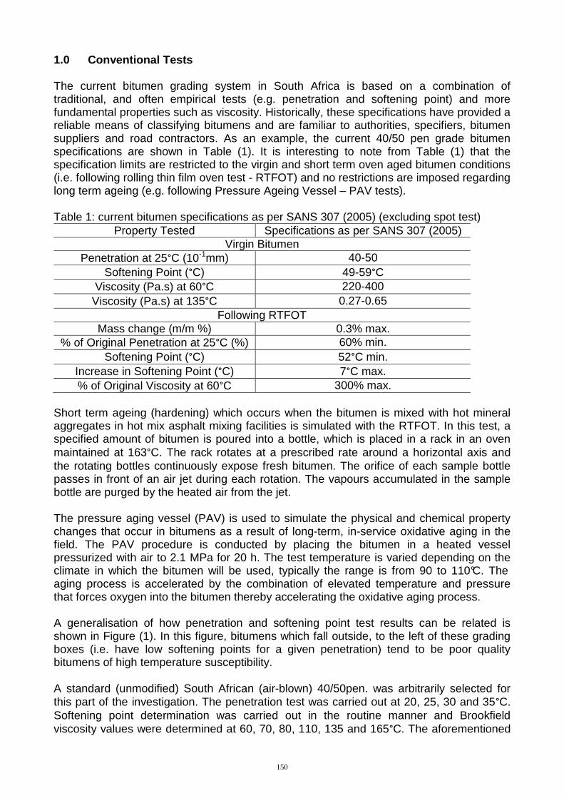
Short term ageing (hardening) which occurs when the bitumen is mixed with hot mineral aggregates in hot mix asphalt mixing facilities is simulated with the RTFOT. In this test, a specified amount of bitumen is poured into a bottle, which is placed in a rack in an oven maintained at 163°C. The rack rotates at a prescribed rate around a horizontal axis and the rotating bottles continuously expose fresh bitumen. The orifice of each sample bottle passes in front of an air jet during each rotation. The vapours accumulated in the sample bottle are purged by the heated air from the jet. The pressure aging vessel (PAV) is used to simulate the physical and chemical property changes that occur in bitumens as a result of long-term, in-service oxidative aging in the field. The PAV procedure is conducted by placing the bitumen in a heated vessel pressurized with air to 2.1 MPa for 20 h. The test temperature is varied depending on the climate in which the bitumen will be used, typically the range is from 90 to 110°C. The aging process is accelerated by the combination of elevated temperature and pressure that forces oxygen into the bitumen thereby accelerating the oxidative aging process. A generalisation of how penetration and softening point test results can be related is shown in Figure (1). In this figure, bitumens which fall outside, to the left of these grading boxes (i.e. have low softening points for a given penetration) tend to be poor quality bitumens of high temperature susceptibility. A standard (unmodified) South African (air-blown) 40/50pen. was arbitrarily selected for this part of the investigation. The penetration test was carried out at 20, 25, 30 and 35°C. Softening point determination was carried out in the routine manner and Brookfield viscosity values were determined at 60, 70, 80, 110, 135 and 165°C. The aforementioned

150

tests were conducted on virgin and RTFOT aged samples. Additionally, standard penetration (25°C) and softening point tests were carried out on PAV aged samples.

Figure 1: Generalised example of penetration versus softening point specification

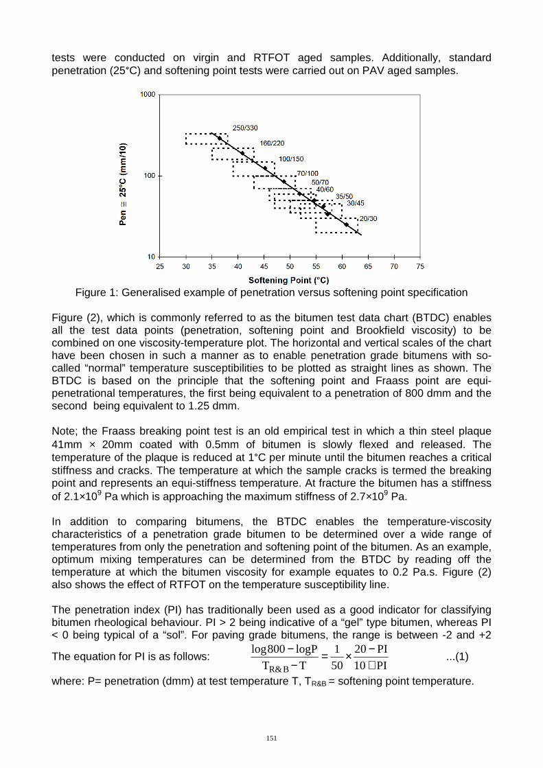
Figure (2), which is commonly referred to as the bitumen test data chart (BTDC) enables all the test data points (penetration, softening point and Brookfield viscosity) to be combined on one viscosity-temperature plot. The horizontal and vertical scales of the chart have been chosen in such a manner as to enable penetration grade bitumens with so-called “normal” temperature susceptibilities to be plotted as straight lines as shown. The BTDC is based on the principle that the softening point and Fraass point are equi-penetrational temperatures, the first being equivalent to a penetration of 800 dmm and the second being equivalent to 1.25 dmm. Note; the Fraass breaking point test is an old empirical test in which a thin steel plaque 41mm × 20mm coated with 0.5mm of bitumen is slowly flexed and released. The temperature of the plaque is reduced at 1°C per minute until the bitumen reaches a critical stiffness and cracks. The temperature at which the sample cracks is termed the breaking point and represents an equi-stiffness temperature. At fracture the bitumen has a stiffness of 2.1×109 Pa which is approaching the maximum stiffness of 2.7×109 Pa. In addition to comparing bitumens, the BTDC enables the temperature-viscosity characteristics of a penetration grade bitumen to be determined over a wide range of temperatures from only the penetration and softening point of the bitumen. As an example, optimum mixing temperatures can be determined from the BTDC by reading off the temperature at which the bitumen viscosity for example equates to 0.2 Pa.s. Figure (2) also shows the effect of RTFOT on the temperature susceptibility line. The penetration index (PI) has traditionally been used as a good indicator for classifying bitumen rheological behaviour. PI > 2 being indicative of a “gel” type bitumen, whereas PI < 0 being typical of a “sol”. For paving grade bitumens, the range is between -2 and +2

The equation for PI is as follows: PI10

PI20

50

1

TT

logP800log

BR& +−×=

−−

...(1)

where: P= penetration (dmm) at test temperature T, TR&B = softening point temperature.

151

As shown in Figure (3), good correlations can be obtained between the softening points and the dynamic viscosity values at 60°C (r 2 = 0.94) and 135°C (r 2 = 0.84) for a range of unmodified and polymer modified bitumens (Páez et al., 2004).

PI

PI focal point

Penetration, dmm

12

5102050

100200

5001000

100000

10000

1000

5

502010

100

Viscosity,Pa.s

2

1

0.5

0.2

0.12502252001751501251007550250-25-50

Temperature, C

Softening point (ASTM), C

Figure 2: Bitumen test data chart showing test data from a 40/50 pen grade bitumen both

in the virgin (lower line) and RTFOT aged conditions (upper line).

Figure 3: Relationship between dynamic viscosity and softening points

More recently (Zolotarev et al., 2004) argued that a more reliable method of treating traditional bitumen test data was by determining the mid point between the Softening point (TS) and Fraass breaking point temperatures (TF). This mid point was referred to as the “reduction temperature TR”, and can be easily calculated for any test temperature (TT) as follows: TR = TT – (TS + TF)/2 ...(2)

152

Figure (4) shows the relationships between penetration (log pen.) and reduction temperature (TR). The upper dashed boundary line represents the softening point (or temperature at a penetration value of 800dmm), whilst the lower dashed boundary line represents the Fraass breaking point temperature (or temperature at a penetration value of 1.25dmm). The family of sloping straight lines represent measured penetration values for a range of bitumens (34 bitumen types tested) having Penetration Index (PI) values ranging from -2.0 to +2.0. It must be noted that in this representation, all generalized straight lines are symmetric about a reduction temperature TR being equal to 0°C. It was found that for all bitumens tested, the axis of symmetry (i.e. TR = 0°C) corresponds to a penetration value of 31dmm. Thus, the temperature corresponding to the middle of PI was shown to be an equi-penetrational value. T31 = (TS + TF)/2 ...(3)

0

0.5

1

1.5

2

2.5

3

-50 -40 -30 -20 -10 0 10 20 30 40 50

Log Pen.

Reduction Temperature Tr

PI-2.0

-1.0

0.0

+1.0

+2.0

Figure 4: Generalised dependency of penetration (log pen.) on reduced temperature (Tr)

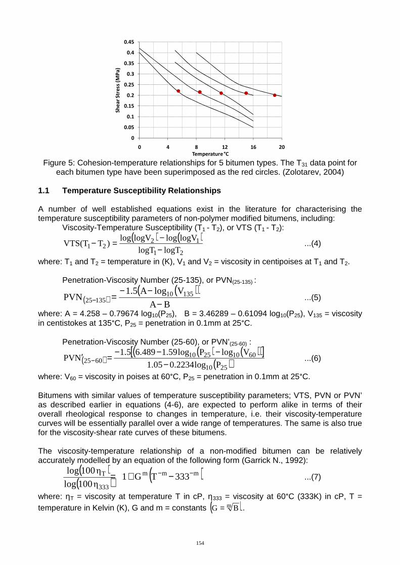
for bitumens with different penetration indices (PI). (Zolotarev, 2004) To appreciate the physical significance of T31, (Zolotarev 2004) conducted the penetration test on a range of bitumen types at a range of test temperatures, in addition to the standard softening point determination. A plot of measured penetration v.s. test temperature allowed the values at which the penetration equates to 31dmm to be determined for each bitumen type (i.e. T31). In the following stage, the investigators conducted parallel plate shear testing at a range of temperatures on 200μm thick bitumen specimens at a shear rate of 1s-1. The shear stress (or cohesion) v.s. temperature profiles are shown for 5 bitumen specimens in Figure (5). The figure also shows the T31 data point for each bitumen type (red circles), which interestingly align themselves very close to a single shear stress or cohesion value. The experiment thus proved that the equi-penetrational temperature T31 is also an equiviscous temperature.

153

0

0.05

0.1

0.15

0.2

0.25

0.3

0.35

0.4

0.45

0 4 8 12 16 20

Sh

ea

r S

tre

ss (

MP

a)

Temperature °C Figure 5: Cohesion-temperature relationships for 5 bitumen types. The T31 data point for

each bitumen type have been superimposed as the red circles. (Zolotarev, 2004) 1.1 Temperature Susceptibility Relationships A number of well established equations exist in the literature for characterising the temperature susceptibility parameters of non-polymer modified bitumens, including:

Viscosity-Temperature Susceptibility (T1 - T2), or VTS (T1 - T2):

( ) ( )

21

1221 logTlogT

logVloglogVlog)TVTS(T

−−=− ...(4)

where: T1 and T2 = temperature in (K), V1 and V2 = viscosity in centipoises at T1 and T2.

Penetration-Viscosity Number (25-135), or PVN(25-135) :

( )( )( )

BA

VlogA1.5PVN 13510

13525 −−−

=− ...(5)

where: A = 4.258 – 0.79674 log10(P25), B = 3.46289 – 0.61094 log10(P25), V135 = viscosity in centistokes at 135°C, P25 = penetration in 0.1mm at 25°C.

Penetration-Viscosity Number (25-60), or PVN’(25-60) :

( )( ) ( )( )[ ]

( )2510

601025106025 Plog0.22341.05

VlogPlog1.596.4891.5NPV

−−−−

=′ − ...(6)

where: V60 = viscosity in poises at 60°C, P25 = penetration in 0.1mm at 25°C. Bitumens with similar values of temperature susceptibility parameters; VTS, PVN or PVN’ as described earlier in equations (4-6), are expected to perform alike in terms of their overall rheological response to changes in temperature, i.e. their viscosity-temperature curves will be essentially parallel over a wide range of temperatures. The same is also true for the viscosity-shear rate curves of these bitumens. The viscosity-temperature relationship of a non-modified bitumen can be relatively accurately modelled by an equation of the following form (Garrick N., 1992):

( )

( ) ( )mmm

333

T 333TG1η100log

η100log −− −+= ...(7)

where: ηT = viscosity at temperature T in cP, η333 = viscosity at 60°C (333K) in cP, T = temperature in Kelvin (K), G and m = constants ( )m BG = .

154

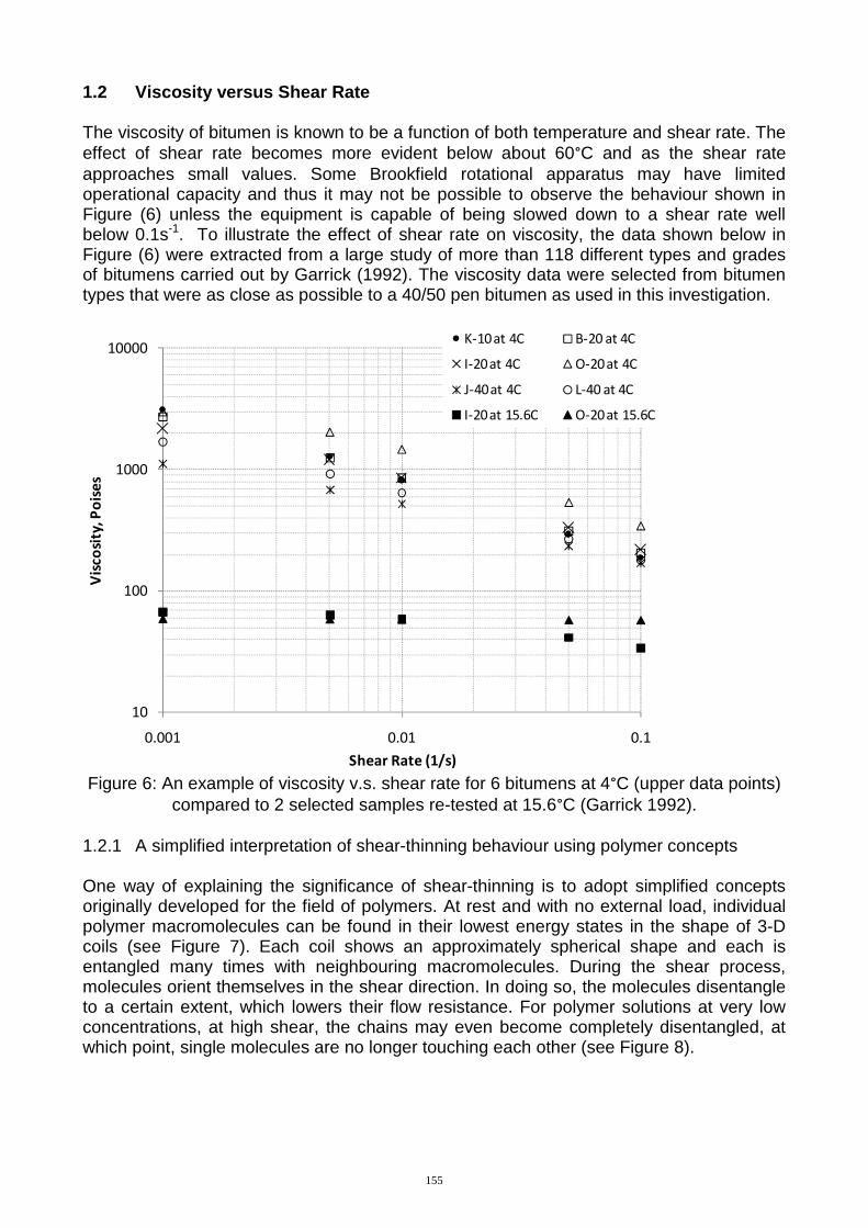
1.2 Viscosity versus Shear Rate The viscosity of bitumen is known to be a function of both temperature and shear rate. The effect of shear rate becomes more evident below about 60°C and as the shear rate approaches small values. Some Brookfield rotational apparatus may have limited operational capacity and thus it may not be possible to observe the behaviour shown in Figure (6) unless the equipment is capable of being slowed down to a shear rate well below 0.1s-1. To illustrate the effect of shear rate on viscosity, the data shown below in Figure (6) were extracted from a large study of more than 118 different types and grades of bitumens carried out by Garrick (1992). The viscosity data were selected from bitumen types that were as close as possible to a 40/50 pen bitumen as used in this investigation.

10

100

1000

10000

0.001 0.01 0.1

Vis

cosi

ty, P

ois

es

Shear Rate (1/s)

K-10 at 4C B-20 at 4C

I-20 at 4C O-20 at 4C

J-40 at 4C L-40 at 4C

I-20 at 15.6C O-20 at 15.6C

Figure 6: An example of viscosity v.s. shear rate for 6 bitumens at 4°C (upper data points)

compared to 2 selected samples re-tested at 15.6°C (Garrick 1992). 1.2.1 A simplified interpretation of shear-thinning behaviour using polymer concepts One way of explaining the significance of shear-thinning is to adopt simplified concepts originally developed for the field of polymers. At rest and with no external load, individual polymer macromolecules can be found in their lowest energy states in the shape of 3-D coils (see Figure 7). Each coil shows an approximately spherical shape and each is entangled many times with neighbouring macromolecules. During the shear process, molecules orient themselves in the shear direction. In doing so, the molecules disentangle to a certain extent, which lowers their flow resistance. For polymer solutions at very low concentrations, at high shear, the chains may even become completely disentangled, at which point, single molecules are no longer touching each other (see Figure 8).

155

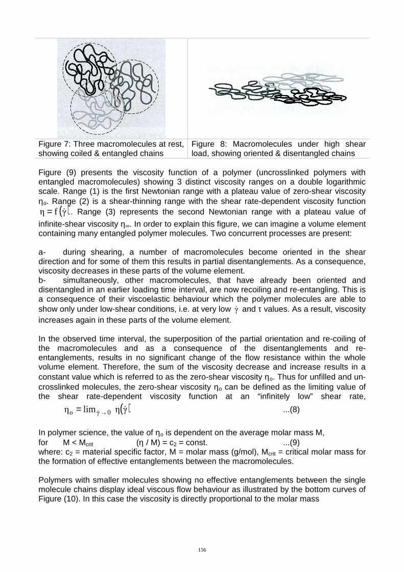
Figure 7: Three macromolecules at rest, showing coiled & entangled chains

Figure 8: Macromolecules under high shear load, showing oriented & disentangled chains

Figure (9) presents the viscosity function of a polymer (uncrosslinked polymers with entangled macromolecules) showing 3 distinct viscosity ranges on a double logarithmic scale. Range (1) is the first Newtonian range with a plateau value of zero-shear viscosity ηo. Range (2) is a shear-thinning range with the shear rate-dependent viscosity function

( )γfη &= . Range (3) represents the second Newtonian range with a plateau value of

infinite-shear viscosity η∞. In order to explain this figure, we can imagine a volume element containing many entangled polymer molecules. Two concurrent processes are present: a- during shearing, a number of macromolecules become oriented in the shear direction and for some of them this results in partial disentanglements. As a consequence, viscosity decreases in these parts of the volume element. b- simultaneously, other macromolecules, that have already been oriented and disentangled in an earlier loading time interval, are now recoiling and re-entangling. This is a consequence of their viscoelastic behaviour which the polymer molecules are able to show only under low-shear conditions, i.e. at very low γ& and τ values. As a result, viscosity increases again in these parts of the volume element. In the observed time interval, the superposition of the partial orientation and re-coiling of the macromolecules and as a consequence of the disentanglements and re-entanglements, results in no significant change of the flow resistance within the whole volume element. Therefore, the sum of the viscosity decrease and increase results in a constant value which is referred to as the zero-shear viscosity ηo. Thus for unfilled and un-crosslinked molecules, the zero-shear viscosity ηo can be defined as the limiting value of the shear rate-dependent viscosity function at an “infinitely low” shear rate,

( )γηlimη 0γo &&→=

...(8)

In polymer science, the value of ηo is dependent on the average molar mass M, for M < Mcrit (η / M) = c2 = const. ...(9) where: c2 = material specific factor, M = molar mass (g/mol), Mcrit = critical molar mass for the formation of effective entanglements between the macromolecules. Polymers with smaller molecules showing no effective entanglements between the single molecule chains display ideal viscous flow behaviour as illustrated by the bottom curves of Figure (10). In this case the viscosity is directly proportional to the molar mass

156

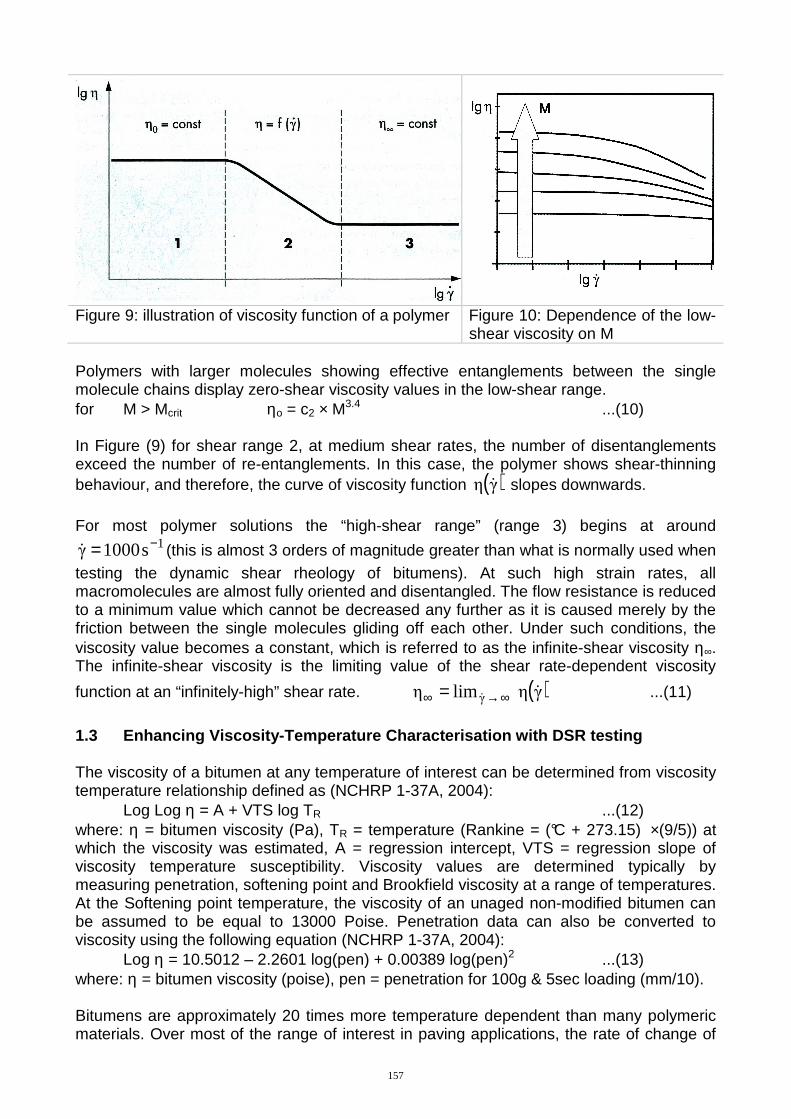
Figure 9: illustration of viscosity function of a polymer Figure 10: Dependence of the low-shear viscosity on M

Polymers with larger molecules showing effective entanglements between the single molecule chains display zero-shear viscosity values in the low-shear range. for M > Mcrit ηo = c2 × M3.4 ...(10)

In Figure (9) for shear range 2, at medium shear rates, the number of disentanglements exceed the number of re-entanglements. In this case, the polymer shows shear-thinning behaviour, and therefore, the curve of viscosity function ( )γη & slopes downwards. For most polymer solutions the “high-shear range” (range 3) begins at around

1s1000γ −=& (this is almost 3 orders of magnitude greater than what is normally used when testing the dynamic shear rheology of bitumens). At such high strain rates, all macromolecules are almost fully oriented and disentangled. The flow resistance is reduced to a minimum value which cannot be decreased any further as it is caused merely by the friction between the single molecules gliding off each other. Under such conditions, the viscosity value becomes a constant, which is referred to as the infinite-shear viscosity η∞. The infinite-shear viscosity is the limiting value of the shear rate-dependent viscosity

function at an “infinitely-high” shear rate. ( )γηlimη γ && ∞→∞ = ...(11)

1.3 Enhancing Viscosity-Temperature Characterisation with DSR testing The viscosity of a bitumen at any temperature of interest can be determined from viscosity temperature relationship defined as (NCHRP 1-37A, 2004):

Log Log η = A + VTS log TR ...(12) where: η = bitumen viscosity (Pa), TR = temperature (Rankine = (°C + 273.15) ×(9/5)) at which the viscosity was estimated, A = regression intercept, VTS = regression slope of viscosity temperature susceptibility. Viscosity values are determined typically by measuring penetration, softening point and Brookfield viscosity at a range of temperatures. At the Softening point temperature, the viscosity of an unaged non-modified bitumen can be assumed to be equal to 13000 Poise. Penetration data can also be converted to viscosity using the following equation (NCHRP 1-37A, 2004):

Log η = 10.5012 – 2.2601 log(pen) + 0.00389 log(pen)2 ...(13) where: η = bitumen viscosity (poise), pen = penetration for 100g & 5sec loading (mm/10). Bitumens are approximately 20 times more temperature dependent than many polymeric materials. Over most of the range of interest in paving applications, the rate of change of

157

complex modulus (G*) with respect to temperature ranges from 15 to 25 percent/°C. Because of the extreme temperature dependency of bitumens, it is necessary to control the temperature for the rheological testing of bitumens to a much finer degree (± 0.1 °C is recommended) than for most other viscoelastic materials. Oscillatory rheometers (e.g. dynamic shear rheometers (DSR)) are designed to control temperature very accurately during testing. Viscosity values can be obtained at a range of temperatures using a DSR by conducting a temperature sweep typically at a fixed frequency of 1.59Hz (10 rad/s), as

an example: 4.8628

sinδ

1

10

G*η

= ...(14)

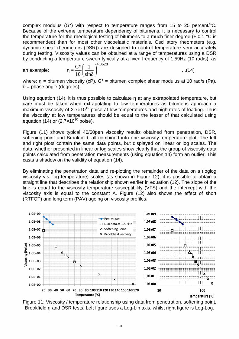
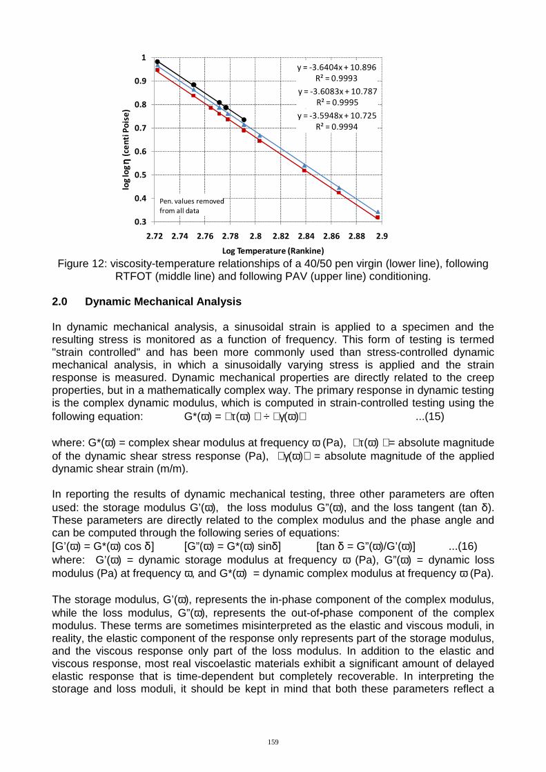
where: η = bitumen viscosity (cP), G* = bitumen complex shear modulus at 10 rad/s (Pa), δ = phase angle (degrees). Using equation (14), it is thus possible to calculate η at any extrapolated temperature, but care must be taken when extrapolating to low temperatures as bitumens approach a maximum viscosity of 2.7×1010 poise at low temperatures and high rates of loading. Thus the viscosity at low temperatures should be equal to the lesser of that calculated using equation (14) or (2.7×1010 poise). Figure (11) shows typical 40/50pen viscosity results obtained from penetration, DSR, softening point and Brookfield, all combined into one viscosity-temperature plot. The left and right plots contain the same data points, but displayed on linear or log scales. The data, whether presented in linear or log scales show clearly that the group of viscosity data points calculated from penetration measurements (using equation 14) form an outlier. This casts a shadow on the validity of equation (14). By eliminating the penetration data and re-plotting the remainder of the data on a (loglog viscosity v.s. log temperature) scales (as shown in Figure 12), it is possible to obtain a straight line that describes the relationship shown earlier in equation (12). The slope of the line is equal to the viscosity temperature susceptibility (VTS) and the intercept with the viscosity axis is equal to the constant A. Figure (12) also shows the effect of short (RTFOT) and long term (PAV) ageing on viscosity profiles.

1.0E+00

1.0E+01

1.0E+02

1.0E+03

1.0E+04

1.0E+05

1.0E+06

1.0E+07

1.0E+08

1.0E+09

20 30 40 50 60 70 80 90 100 110 120 130 140 150 160 170

Vis

cosi

ty (

Po

ise

)

Temperature (°C)

Pen. values

DSR data at 1.59 Hz

Softening Point

Brookfield viscosity

Figure 11: Viscosity / temperature relationship using data from penetration, softening point, Brookfield η and DSR tests. Left figure uses a Log-Lin axis, whilst right figure is Log-Log.

158

y = -3.5948x + 10.725

R² = 0.9994

y = -3.6083x + 10.787

R² = 0.9995

y = -3.6404x + 10.896

R² = 0.9993

0.3

0.4

0.5

0.6

0.7

0.8

0.9

1

2.72 2.74 2.76 2.78 2.8 2.82 2.84 2.86 2.88 2.9

log

log

ηη ηη(c

en

ti P

ois

e)

Log Temperature (Rankine)

Pen. values removed

from all data

Pen. values removed

from all data

Figure 12: viscosity-temperature relationships of a 40/50 pen virgin (lower line), following

RTFOT (middle line) and following PAV (upper line) conditioning. 2.0 Dynamic Mechanical Analysis In dynamic mechanical analysis, a sinusoidal strain is applied to a specimen and the resulting stress is monitored as a function of frequency. This form of testing is termed "strain controlled" and has been more commonly used than stress-controlled dynamic mechanical analysis, in which a sinusoidally varying stress is applied and the strain response is measured. Dynamic mechanical properties are directly related to the creep properties, but in a mathematically complex way. The primary response in dynamic testing is the complex dynamic modulus, which is computed in strain-controlled testing using the following equation: G*(ω) = τ(ω) ÷ γ(ω) ...(15) where: G*(ω) = complex shear modulus at frequency ω (Pa), τ(ω) = absolute magnitude of the dynamic shear stress response (Pa), γ(ω) = absolute magnitude of the applied dynamic shear strain (m/m). In reporting the results of dynamic mechanical testing, three other parameters are often used: the storage modulus G’(ω), the loss modulus G”(ω), and the loss tangent (tan δ). These parameters are directly related to the complex modulus and the phase angle and can be computed through the following series of equations: [G’(ω) = G*(ω) cos δ ] [G”(ω) = G*(ω) sinδ] [tan δ = G”(ω)/G’(ω)] ...(16) where: G’(ω) = dynamic storage modulus at frequency ω (Pa), G”(ω) = dynamic loss modulus (Pa) at frequency ω, and G*(ω) = dynamic complex modulus at frequency ω (Pa). The storage modulus, G’(ω), represents the in-phase component of the complex modulus, while the loss modulus, G”(ω), represents the out-of-phase component of the complex modulus. These terms are sometimes misinterpreted as the elastic and viscous moduli, in reality, the elastic component of the response only represents part of the storage modulus, and the viscous response only part of the loss modulus. In addition to the elastic and viscous response, most real viscoelastic materials exhibit a significant amount of delayed elastic response that is time-dependent but completely recoverable. In interpreting the storage and loss moduli, it should be kept in mind that both these parameters reflect a

159

portion of the delayed elastic response. Therefore, they cannot be strictly interpreted as elastic and viscous moduli and are properly referred to as the storage and loss moduli. Various other viscoelastic functions can be defined through the complex modulus and the phase angle, including: Dynamic complex compliance in shear [J* = 1/G*], Storage compliance in shear [J' = cos δ / G*], Loss compliance in shear [J" = sin δ / G*], Dynamic complex viscosity in shear [η* = G*/ω], Real part of complex viscosity [η' = G"/ω], Imaginary part of complex viscosity [η" = G'/ω]. Note; a distinction is made between dynamic viscosity η* which is determined by oscillatory tests and steady state shear viscosity η whose value is determined by rotational tests under steady shear conditions (i.e. by applying a constant shear rate or a constant shear stress at each single measuring point). It must also be noted that the real part of the complex viscosity is an energy dissipation term similar to the imaginary part of the complex modulus. Other interrelationships between the complex quantities include: [G’ = J’/J2], [J’ = G’/G2],

and

′′′

=′′′

J

J

G

G, where; 222 GGG ′′+′= ...(17)

2.1 Dynamic Shear Rheometer Testing When performing oscillatory tests a rheometer is only capable of producing two independent sets of raw data (see Figures 13 & 14). In the controlled shear strain mode of operation, a preset deflection angle value is input by the operator and the DSR measures the torque T and phase shift angle δ. In rheological terms, the operator inputs the target strain γ(t) [%], and in turn the DSR determines the shear stress τ(t) and δ [°]. From these two independent variables, the elastic (G’) and viscous (G’’) components of the viscoelastic response are determined, and all other viscoelastic functions listed earlier are mathematical conversions of the original two independent sets of raw DSR data. When testing bitumen using a DSR, the following guidelines may be used for selecting plate diameters and sample thickness (gap) (Anderson et al. 1994, Petersen et al. 1994): • 8-mm parallel plates with a 2-mm gap are recommended when 0.1 MPa < G* < 30 MPa, (this typically covers the temperature range from approximately 5 to 35°C). • 25-mm parallel plates with a 1-mm gap are recommended when 1.0 kPa < G* < 100 kPa (i.e. at temperatures above 35°C). • 50-mm parallel plates (less common) are recommended when G* < 1 kPa. The two main types of tests performed during DSR testing are strain sweeps and frequency sweeps. Strain sweeps are used to determine the region of linear behaviour. 2.2 Strain Sweeps Within the linear viscoelastic (LVE) region, the modulus is independent of stress or strain. This independency can be ascertained by applying a varying (gradually increasing) strain to the sample at a constant frequency and test temperature, and observing the resulting stress or modulus. This procedure is often referred to as a strain sweep. For tests with controlled shear strain: ( ) ( )ωtsinγtγ A×= ...(18) The upper limit of the linear region is arbitrarily defined as the point at which the complex (or storage) modulus decreases to 95% of the initial modulus. A typical strain sweep, with a definition of the linear region, is shown in Figure (15). When the LVE limit is plotted

160

against a complex modulus, a reasonable relationship is seen, in which the linear limit increases with decreasing modulus. The results from a large US investigation that included testing more than 40 bitumens at 10 rad/s (1.59Hz), but at different temperatures and aging conditions are shown in figure (16). The plotted points represent the strain level at which the modulus is reduced to 95% of its zero-strain value. Generally, the LVE strain limit increases with temperature and there is a clear relationship between the complex modulus and the linear strain limit which is apparently similar for a wide range of bitumens. Using the data in figure (16) as a guide, the recommendations require the strain to be controlled to ± 20% of the following; γ = 12.0/(G*)0.29, and when testing in the controlled-stress rheometer, the stress should be controlled to ± 20% of the following; τ = 0.12(G*)0.71, (Anderson et al. 1994, Petersen et al. 1994).

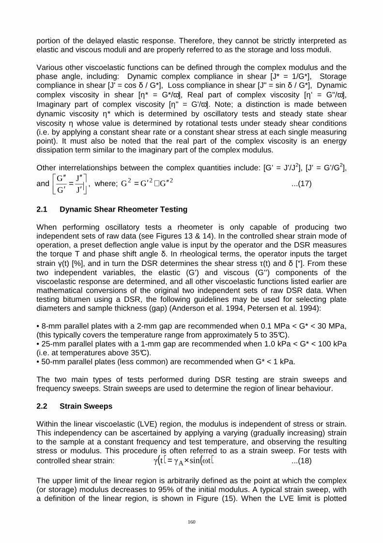
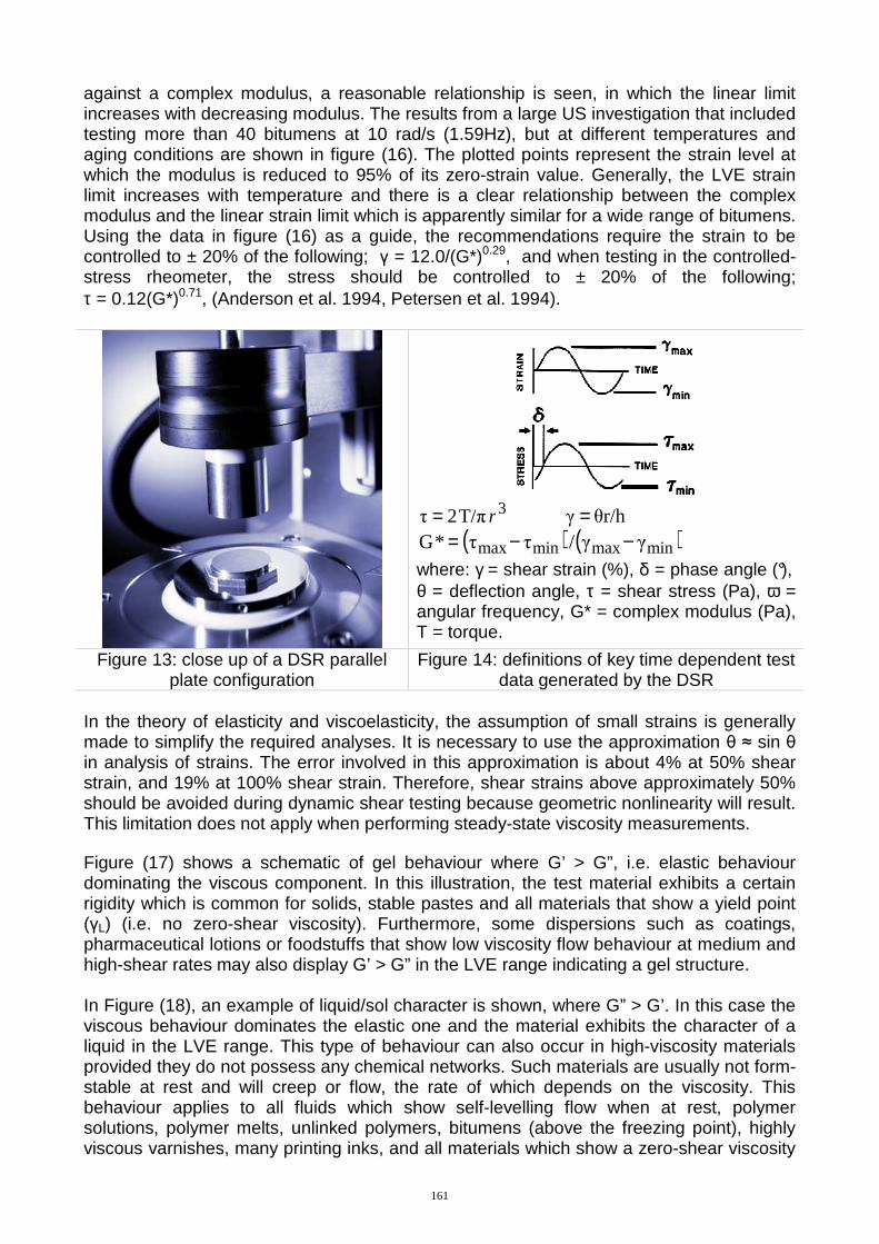
3T/π2τ r= θr/hγ =

( ) ( )minmaxminmax γγ/ττ*G −−=

where: γ = shear strain (%), δ = phase angle (°), θ = deflection angle, τ = shear stress (Pa), ω = angular frequency, G* = complex modulus (Pa), T = torque.

Figure 13: close up of a DSR parallel plate configuration

Figure 14: definitions of key time dependent test data generated by the DSR

In the theory of elasticity and viscoelasticity, the assumption of small strains is generally made to simplify the required analyses. It is necessary to use the approximation θ ≈ sin θ in analysis of strains. The error involved in this approximation is about 4% at 50% shear strain, and 19% at 100% shear strain. Therefore, shear strains above approximately 50% should be avoided during dynamic shear testing because geometric nonlinearity will result. This limitation does not apply when performing steady-state viscosity measurements.

Figure (17) shows a schematic of gel behaviour where G’ > G”, i.e. elastic behaviour dominating the viscous component. In this illustration, the test material exhibits a certain rigidity which is common for solids, stable pastes and all materials that show a yield point (γL) (i.e. no zero-shear viscosity). Furthermore, some dispersions such as coatings, pharmaceutical lotions or foodstuffs that show low viscosity flow behaviour at medium and high-shear rates may also display G’ > G” in the LVE range indicating a gel structure. In Figure (18), an example of liquid/sol character is shown, where G” > G’. In this case the viscous behaviour dominates the elastic one and the material exhibits the character of a liquid in the LVE range. This type of behaviour can also occur in high-viscosity materials provided they do not possess any chemical networks. Such materials are usually not form-stable at rest and will creep or flow, the rate of which depends on the viscosity. This behaviour applies to all fluids which show self-levelling flow when at rest, polymer solutions, polymer melts, unlinked polymers, bitumens (above the freezing point), highly viscous varnishes, many printing inks, and all materials which show a zero-shear viscosity

161

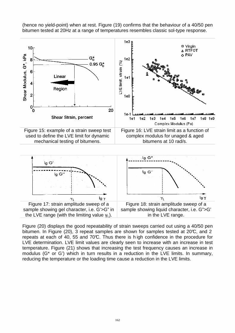
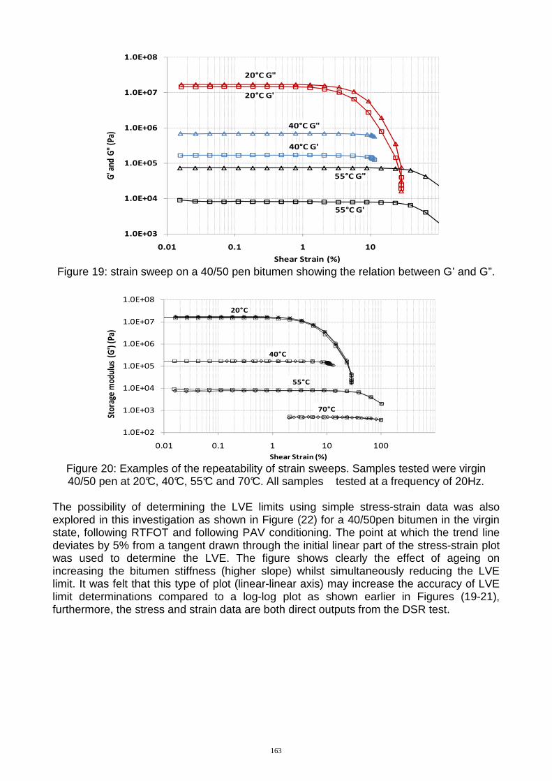
(hence no yield-point) when at rest. Figure (19) confirms that the behaviour of a 40/50 pen bitumen tested at 20Hz at a range of temperatures resembles classic sol-type response.

Figure 15: example of a strain sweep test used to define the LVE limit for dynamic

mechanical testing of bitumens.

Figure 16: LVE strain limit as a function of complex modulus for unaged & aged

bitumens at 10 rad/s.

Figure 17: strain amplitude sweep of a

sample showing gel character, i.e. G’>G” in the LVE range (with the limiting value γL).

Figure 18: strain amplitude sweep of a sample showing liquid character, i.e. G”>G’

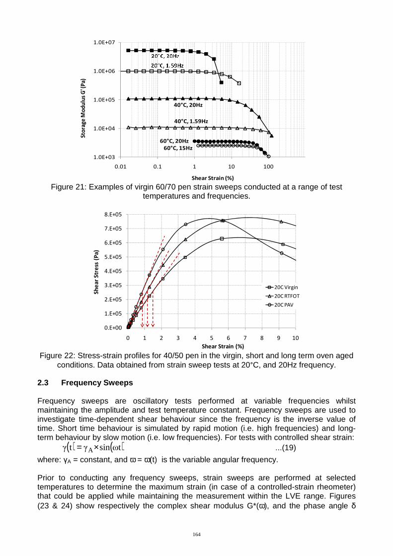
in the LVE range. Figure (20) displays the good repeatability of strain sweeps carried out using a 40/50 pen bitumen. In Figure (20), 3 repeat samples are shown for samples tested at 20°C, and 2 repeats at each of 40, 55 and 70°C. Thus there is h igh confidence in the procedure for LVE determination. LVE limit values are clearly seen to increase with an increase in test temperature. Figure (21) shows that increasing the test frequency causes an increase in modulus (G* or G’) which in turn results in a reduction in the LVE limits. In summary, reducing the temperature or the loading time cause a reduction in the LVE limits.

162

1.0E+03

1.0E+04

1.0E+05

1.0E+06

1.0E+07

1.0E+08

0.01 0.1 1 10

G' a

nd G

" (P

a)

Shear Strain (%)

20°C G'

40°C G"

40°C G'

55°C G"

55°C G'

20°C G"

Figure 19: strain sweep on a 40/50 pen bitumen showing the relation between G’ and G”.

1.0E+02

1.0E+03

1.0E+04

1.0E+05

1.0E+06

1.0E+07

1.0E+08

0.01 0.1 1 10 100

Stor

age

mod

ulus

(G

') (P

a)

Shear Strain (%)

20°C

40°C

55°C

70°C

Figure 20: Examples of the repeatability of strain sweeps. Samples tested were virgin 40/50 pen at 20°C, 40°C, 55°C and 70°C. All samples tested at a frequency of 20Hz.

The possibility of determining the LVE limits using simple stress-strain data was also explored in this investigation as shown in Figure (22) for a 40/50pen bitumen in the virgin state, following RTFOT and following PAV conditioning. The point at which the trend line deviates by 5% from a tangent drawn through the initial linear part of the stress-strain plot was used to determine the LVE. The figure shows clearly the effect of ageing on increasing the bitumen stiffness (higher slope) whilst simultaneously reducing the LVE limit. It was felt that this type of plot (linear-linear axis) may increase the accuracy of LVE limit determinations compared to a log-log plot as shown earlier in Figures (19-21), furthermore, the stress and strain data are both direct outputs from the DSR test.

163

1.0E+03

1.0E+04

1.0E+05

1.0E+06

1.0E+07

0.01 0.1 1 10 100

Sto

rage

Mo

du

lus

G' (

Pa)

Shear Strain (%)

40°C, 20Hz

60°C, 15Hz

60°C, 20Hz

40°C, 1.59Hz

Figure 21: Examples of virgin 60/70 pen strain sweeps conducted at a range of test

temperatures and frequencies.

0.E+00

1.E+05

2.E+05

3.E+05

4.E+05

5.E+05

6.E+05

7.E+05

8.E+05

0 1 2 3 4 5 6 7 8 9 10

Sh

ea

r S

tre

ss (

Pa

)

Shear Strain (%)

20C Virgin

20C RTFOT

20C PAV

Figure 22: Stress-strain profiles for 40/50 pen in the virgin, short and long term oven aged

conditions. Data obtained from strain sweep tests at 20°C, and 20Hz frequency.

2.3 Frequency Sweeps Frequency sweeps are oscillatory tests performed at variable frequencies whilst maintaining the amplitude and test temperature constant. Frequency sweeps are used to investigate time-dependent shear behaviour since the frequency is the inverse value of time. Short time behaviour is simulated by rapid motion (i.e. high frequencies) and long-term behaviour by slow motion (i.e. low frequencies). For tests with controlled shear strain: ( ) ( )ωtsinγtγ A×= ...(19)

where: γA = constant, and ω = ω(t) is the variable angular frequency. Prior to conducting any frequency sweeps, strain sweeps are performed at selected temperatures to determine the maximum strain (in case of a controlled-strain rheometer) that could be applied while maintaining the measurement within the LVE range. Figures (23 & 24) show respectively the complex shear modulus G*(ω), and the phase angle δ

164

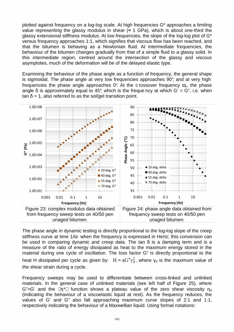
plotted against frequency on a log-log scale. At high frequencies G* approaches a limiting value representing the glassy modulus in shear (≈ 1 GPa), which is about one-third the glassy extensional stiffness modulus. At low frequencies, the slope of the log-log plot of G* versus frequency approaches 1:1, which signifies that viscous flow has been reached, and that the bitumen is behaving as a Newtonian fluid. At intermediate frequencies, the behaviour of the bitumen changes gradually from that of a simple fluid to a glassy solid. In this intermediate region, centred around the intersection of the glassy and viscous asymptotes, much of the deformation will be of the delayed elastic type. Examining the behaviour of the phase angle as a function of frequency, the general shape is sigmoidal. The phase angle at very low frequencies approaches 90°, and at very high frequencies the phase angle approaches 0°. At the c rossover frequency ωc, the phase angle δ is approximately equal to 45°, which is the freque ncy at which G’ = G”, i.e. when tan δ = 1, also referred to as the sol/gel transition point.

1.0E+01

1.0E+02

1.0E+03

1.0E+04

1.0E+05

1.0E+06

1.0E+07

1.0E+08

0.001 0.01 0.1 1 10

G*

(P

a)

Frequency (Hz)

20 deg. G*

40 deg. G*

55 deg. G*

70 deg. G*

35

40

45

50

55

60

65

70

75

80

85

90

0.001 0.01 0.1 1 10

Ph

ase

An

gle

(°C

)

Frequency (Hz)

20 deg. delta

40 deg. delta

55 deg. delta

70 deg. delta

Figure 23: complex modulus data obtained from frequency sweep tests on 40/50 pen

unaged bitumen.

Figure 24: phase angle data obtained from frequency sweep tests on 40/50 pen

unaged bitumen. The phase angle in dynamic testing is directly proportional to the log-log slope of the creep stiffness curve at time 1/ω when the frequency is expressed in Hertz; this conversion can be used in comparing dynamic and creep data. The tan δ is a damping term and is a measure of the ratio of energy dissipated as heat to the maximum energy stored in the material during one cycle of oscillation. The loss factor G” is directly proportional to the

heat H dissipated per cycle as given by: 20γGπH ′′= , where γ0 is the maximum value of

the shear strain during a cycle. Frequency sweeps may be used to differentiate between cross-linked and unlinked materials. In the general case of unlinked materials (see left half of Figure 25), where G”>G’ and the η* function shows a plateau value of the zero shear viscosity η0 (indicating the behaviour of a viscoelastic liquid at rest). As the frequency reduces, the values of G’ and G” also fall approaching maximum curve slopes of 2:1 and 1:1, respectively indicating the behaviour of a Maxwellian liquid. Using formal notations:

165

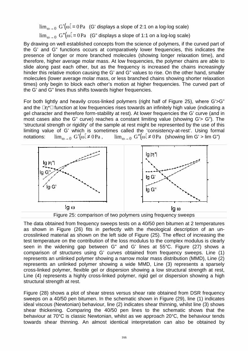
( ) Pa0ωGlim 0ω =′→ (G’ displays a slope of 2:1 on a log-log scale)

( ) Pa0ωGlim 0ω =′′→ (G” displays a slope of 1:1 on a log-log scale)

By drawing on well established concepts from the science of polymers, if the curved part of the G’ and G” functions occurs at comparatively lower frequencies, this indicates the presence of longer or more branched molecules (showing longer relaxation time), and therefore, higher average molar mass. At low frequencies, the polymer chains are able to slide along past each other, but as the frequency is increased the chains increasingly hinder this relative motion causing the G’ and G” values to rise. On the other hand, smaller molecules (lower average molar mass, or less branched chains showing shorter relaxation times) only begin to block each other’s motion at higher frequencies. The curved part of the G’ and G” lines thus shifts towards higher frequencies. For both lightly and heavily cross-linked polymers (right half of Figure 25), where G’>G” and the η* function at low frequencies rises towards an infinitely high value (indicating a gel character and therefore form-stability at rest). At lower frequencies the G’ curve (and in most cases also the G” curve) reaches a constant limiting value (showing G’> G”). The ‘structural strength or rigidity’ of the sample at rest might be represented by the use of this limiting value of G’ which is sometimes called the ‘consistency-at-rest’. Using formal notations: ( ) Pa0ωGlim 0ω ≠′→ , ( ) Pa0ωGlim 0ω ≠′′→ (showing lim G’ > lim G”)

Figure 25: comparison of two polymers using frequency sweeps

The data obtained from frequency sweeps tests on a 40/50 pen bitumen at 2 temperatures as shown in Figure (26) fits in perfectly with the rheological description of an un-crosslinked material as shown on the left side of Figure (25). The effect of increasing the test temperature on the contribution of the loss modulus to the complex modulus is clearly seen in the widening gap between G” and G’ lines at 55°C. Figure (27) shows a comparison of structures using G’ curves obtained from frequency sweeps. Line (1) represents an unlinked polymer showing a narrow molar mass distribution (MMD), Line (2) represents an unlinked polymer showing a wide MMD, Line (3) represents a sparsely cross-linked polymer, flexible gel or dispersion showing a low structural strength at rest, Line (4) represents a highly cross-linked polymer, rigid gel or dispersion showing a high structural strength at rest. Figure (28) shows a plot of shear stress versus shear rate obtained from DSR frequency sweeps on a 40/50 pen bitumen. In the schematic shown in Figure (29), line (1) indicates ideal viscous (Newtonian) behaviour, line (2) indicates shear thinning, whilst line (3) shows shear thickening. Comparing the 40/50 pen lines to the schematic shows that the behaviour at 70°C is classic Newtonian, whilst as we approach 20°C, the behaviour tends towards shear thinning. An almost identical interpretation can also be obtained by

166

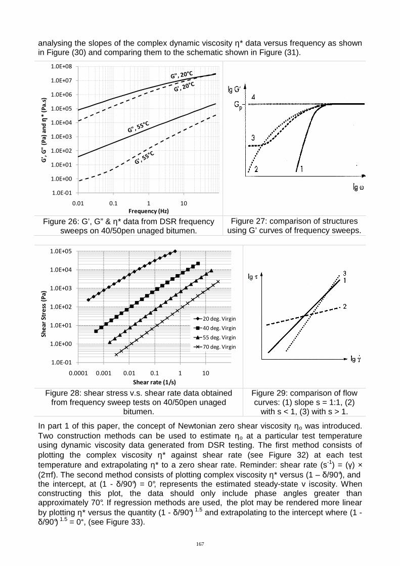
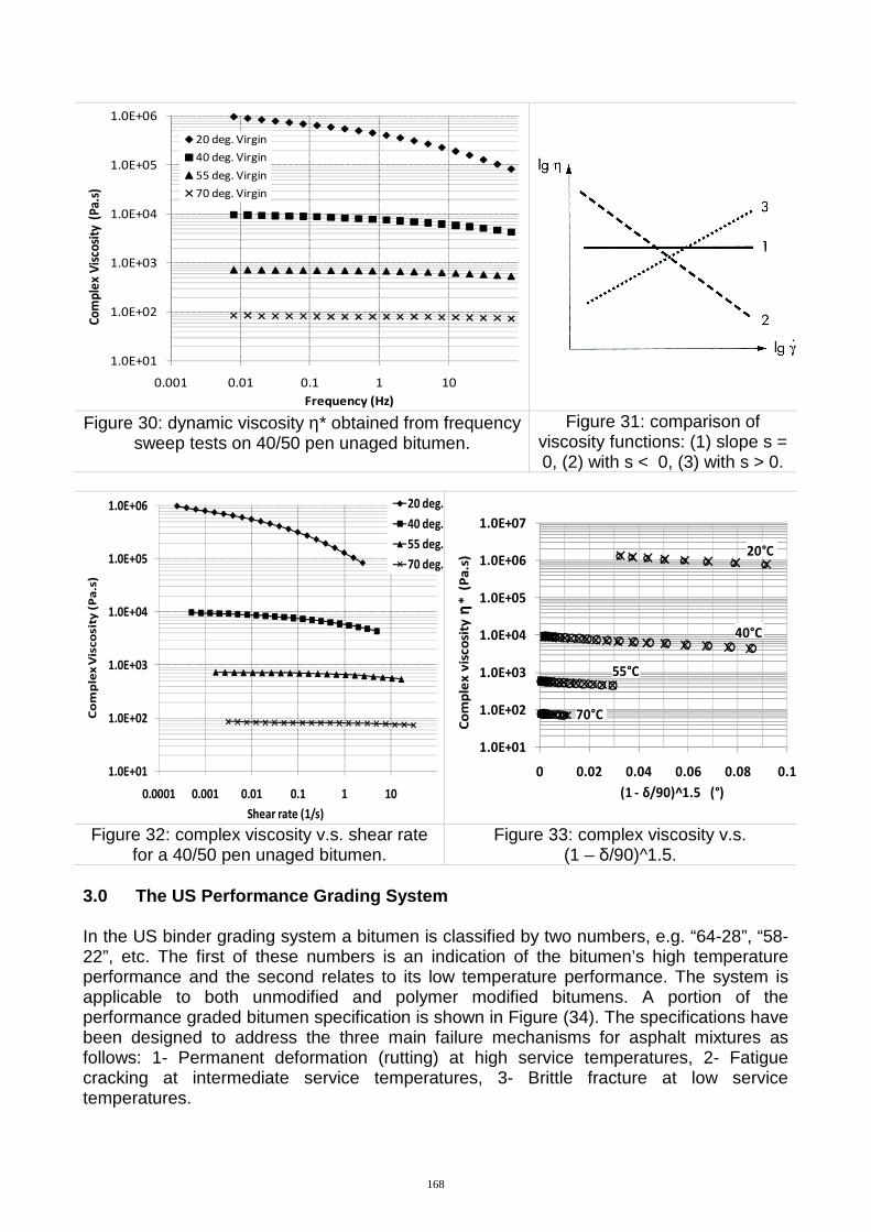
analysing the slopes of the complex dynamic viscosity η* data versus frequency as shown in Figure (30) and comparing them to the schematic shown in Figure (31).

1.0E-01

1.0E+00

1.0E+01

1.0E+02

1.0E+03

1.0E+04

1.0E+05

1.0E+06

1.0E+07

1.0E+08

0.01 0.1 1 10

G',

G"

(Pa

) a

nd

ηη ηη*

(P

a.s

)

Frequency (Hz)

Figure 26: G’, G” & η* data from DSR frequency sweeps on 40/50pen unaged bitumen.

Figure 27: comparison of structures using G’ curves of frequency sweeps.

1.0E-01

1.0E+00

1.0E+01

1.0E+02

1.0E+03

1.0E+04

1.0E+05

0.0001 0.001 0.01 0.1 1 10

Sh

ea

r S

tre

ss (

Pa

)

Shear rate (1/s)

20 deg. Virgin

40 deg. Virgin

55 deg. Virgin

70 deg. Virgin

Figure 28: shear stress v.s. shear rate data obtained from frequency sweep tests on 40/50pen unaged

bitumen.

Figure 29: comparison of flow curves: (1) slope s = 1:1, (2)

with s < 1, (3) with s > 1.

In part 1 of this paper, the concept of Newtonian zero shear viscosity ηo was introduced. Two construction methods can be used to estimate ηo at a particular test temperature using dynamic viscosity data generated from DSR testing. The first method consists of plotting the complex viscosity η* against shear rate (see Figure 32) at each test temperature and extrapolating η* to a zero shear rate. Reminder: shear rate (s-1) = (γ) × (2πf). The second method consists of plotting complex viscosity η* versus (1 – δ/90°), and the intercept, at (1 - δ/90°) = 0°, represents the estimated steady-state v iscosity. When constructing this plot, the data should only include phase angles greater than approximately 70°. If regression methods are used, the plot may be rendered more linear by plotting η* versus the quantity (1 - δ/90°) 1.5 and extrapolating to the intercept where (1 - δ/90°) 1.5 = 0°, (see Figure 33).

167

1.0E+01

1.0E+02

1.0E+03

1.0E+04

1.0E+05

1.0E+06

0.001 0.01 0.1 1 10

Co

mp

lex

Vis

cosi

ty (

Pa

.s)

Frequency (Hz)

20 deg. Virgin

40 deg. Virgin

55 deg. Virgin

70 deg. Virgin

Figure 30: dynamic viscosity η* obtained from frequency sweep tests on 40/50 pen unaged bitumen.

Figure 31: comparison of viscosity functions: (1) slope s = 0, (2) with s < 0, (3) with s > 0.

1.0E+01

1.0E+02

1.0E+03

1.0E+04

1.0E+05

1.0E+06

0.0001 0.001 0.01 0.1 1 10

Co

mp

lex

Vis

co

sit

y (

Pa

.s)

Shear rate (1/s)

20 deg.

40 deg.

55 deg.

70 deg.

1.0E+01

1.0E+02

1.0E+03

1.0E+04

1.0E+05

1.0E+06

1.0E+07

0 0.02 0.04 0.06 0.08 0.1

Co

mp

lex

vis

co

sity

ηη ηη*

(P

a.s

)

(1 - δ/90)^1.5 (°)

20°C

55°C

40°C

70°C

Figure 32: complex viscosity v.s. shear rate for a 40/50 pen unaged bitumen.

Figure 33: complex viscosity v.s. (1 – δ/90)^1.5.

3.0 The US Performance Grading System In the US binder grading system a bitumen is classified by two numbers, e.g. “64-28”, “58-22”, etc. The first of these numbers is an indication of the bitumen’s high temperature performance and the second relates to its low temperature performance. The system is applicable to both unmodified and polymer modified bitumens. A portion of the performance graded bitumen specification is shown in Figure (34). The specifications have been designed to address the three main failure mechanisms for asphalt mixtures as follows: 1- Permanent deformation (rutting) at high service temperatures, 2- Fatigue cracking at intermediate service temperatures, 3- Brittle fracture at low service temperatures.

168

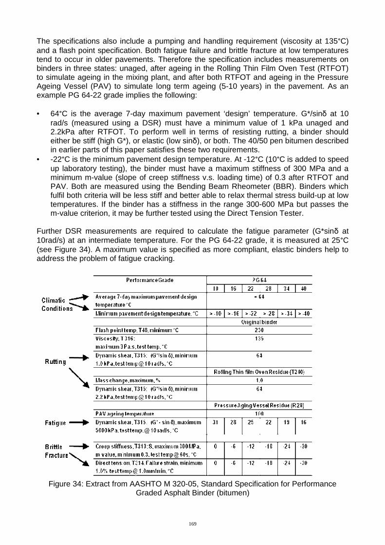
The specifications also include a pumping and handling requirement (viscosity at 135°C) and a flash point specification. Both fatigue failure and brittle fracture at low temperatures tend to occur in older pavements. Therefore the specification includes measurements on binders in three states: unaged, after ageing in the Rolling Thin Film Oven Test (RTFOT) to simulate ageing in the mixing plant, and after both RTFOT and ageing in the Pressure Ageing Vessel (PAV) to simulate long term ageing (5-10 years) in the pavement. As an example PG 64-22 grade implies the following: • 64°C is the average 7-day maximum pavement ‘design’ temperature. G*/sinδ at 10

rad/s (measured using a DSR) must have a minimum value of 1 kPa unaged and 2.2kPa after RTFOT. To perform well in terms of resisting rutting, a binder should either be stiff (high G*), or elastic (low sinδ), or both. The 40/50 pen bitumen described in earlier parts of this paper satisfies these two requirements.

• -22°C is the minimum pavement design temperature. At -12°C (10°C is added to speed up laboratory testing), the binder must have a maximum stiffness of 300 MPa and a minimum m-value (slope of creep stiffness v.s. loading time) of 0.3 after RTFOT and PAV. Both are measured using the Bending Beam Rheometer (BBR). Binders which fulfil both criteria will be less stiff and better able to relax thermal stress build-up at low temperatures. If the binder has a stiffness in the range 300-600 MPa but passes the m-value criterion, it may be further tested using the Direct Tension Tester.

Further DSR measurements are required to calculate the fatigue parameter (G*sinδ at 10rad/s) at an intermediate temperature. For the PG 64-22 grade, it is measured at 25°C (see Figure 34). A maximum value is specified as more compliant, elastic binders help to address the problem of fatigue cracking.

Figure 34: Extract from AASHTO M 320-05, Standard Specification for Performance

Graded Asphalt Binder (bitumen)

169

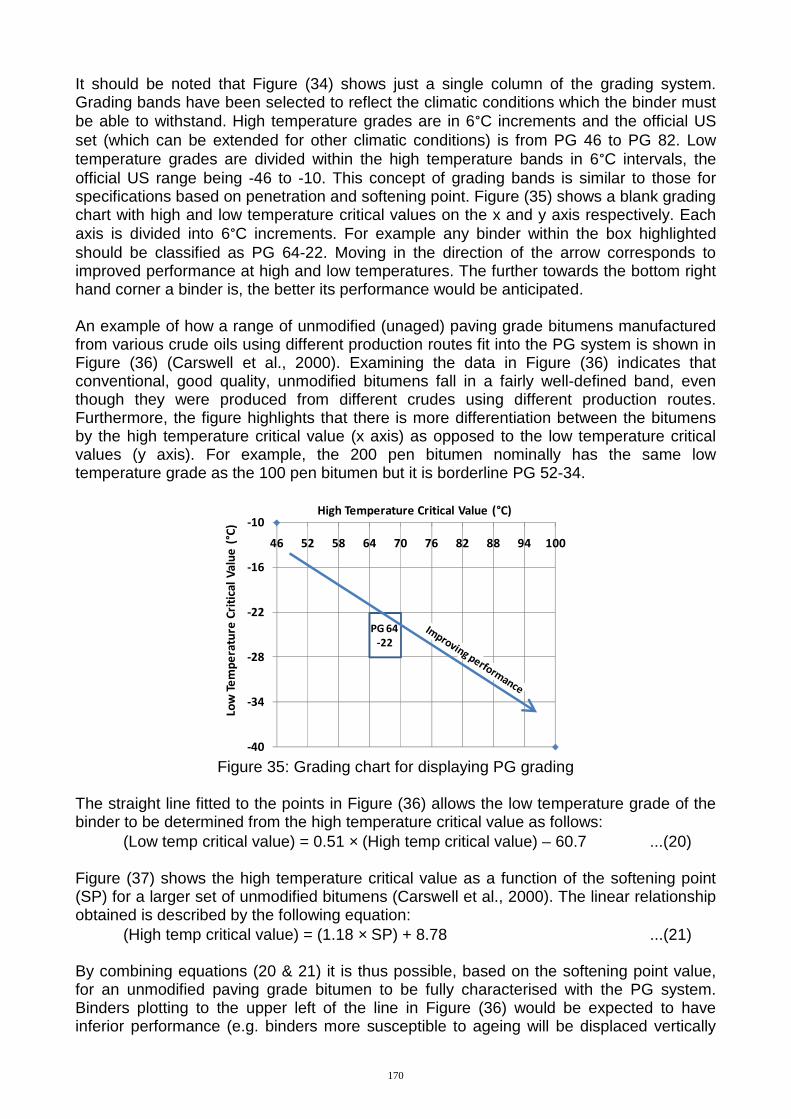
It should be noted that Figure (34) shows just a single column of the grading system. Grading bands have been selected to reflect the climatic conditions which the binder must be able to withstand. High temperature grades are in 6°C increments and the official US set (which can be extended for other climatic conditions) is from PG 46 to PG 82. Low temperature grades are divided within the high temperature bands in 6°C intervals, the official US range being -46 to -10. This concept of grading bands is similar to those for specifications based on penetration and softening point. Figure (35) shows a blank grading chart with high and low temperature critical values on the x and y axis respectively. Each axis is divided into 6°C increments. For example any binder within the box highlighted should be classified as PG 64-22. Moving in the direction of the arrow corresponds to improved performance at high and low temperatures. The further towards the bottom right hand corner a binder is, the better its performance would be anticipated. An example of how a range of unmodified (unaged) paving grade bitumens manufactured from various crude oils using different production routes fit into the PG system is shown in Figure (36) (Carswell et al., 2000). Examining the data in Figure (36) indicates that conventional, good quality, unmodified bitumens fall in a fairly well-defined band, even though they were produced from different crudes using different production routes. Furthermore, the figure highlights that there is more differentiation between the bitumens by the high temperature critical value (x axis) as opposed to the low temperature critical values (y axis). For example, the 200 pen bitumen nominally has the same low temperature grade as the 100 pen bitumen but it is borderline PG 52-34.

-40

-34

-28

-22

-16

-10

46 52 58 64 70 76 82 88 94 100

Low

Te

mp

era

ture

Cri

tica

l V

alu

e (

°C)

High Temperature Critical Value (°C)

PG 64

-22

Figure 35: Grading chart for displaying PG grading

The straight line fitted to the points in Figure (36) allows the low temperature grade of the binder to be determined from the high temperature critical value as follows: (Low temp critical value) = 0.51 × (High temp critical value) – 60.7 ...(20) Figure (37) shows the high temperature critical value as a function of the softening point (SP) for a larger set of unmodified bitumens (Carswell et al., 2000). The linear relationship obtained is described by the following equation: (High temp critical value) = (1.18 × SP) + 8.78 ...(21) By combining equations (20 & 21) it is thus possible, based on the softening point value, for an unmodified paving grade bitumen to be fully characterised with the PG system. Binders plotting to the upper left of the line in Figure (36) would be expected to have inferior performance (e.g. binders more susceptible to ageing will be displaced vertically

170

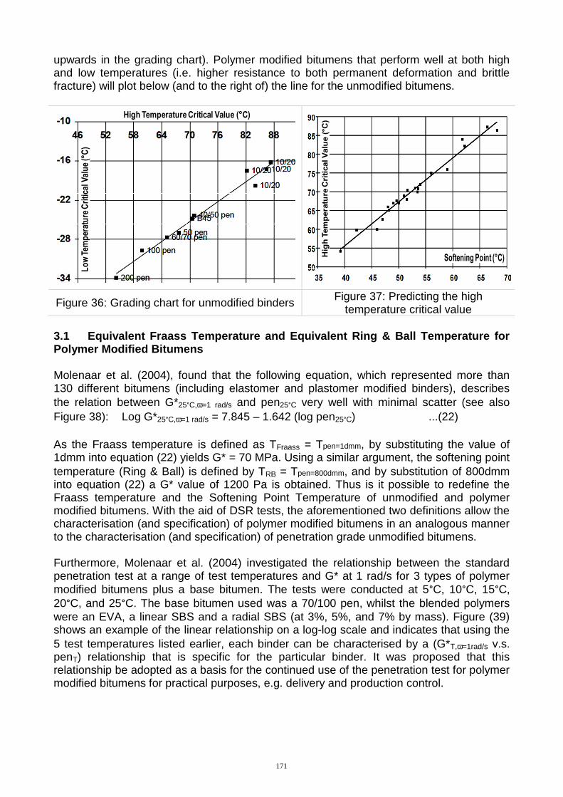
upwards in the grading chart). Polymer modified bitumens that perform well at both high and low temperatures (i.e. higher resistance to both permanent deformation and brittle fracture) will plot below (and to the right of) the line for the unmodified bitumens.

Lo

w T

emp

erat

ure

Cri

tica

l Val

ue

(°C

)

High Temperature Critical Value (°C)

Softening Point (°C)Hig

h T

em

pera

ture

Cri

tical V

alu

e (

°C)

Figure 36: Grading chart for unmodified binders Figure 37: Predicting the high temperature critical value

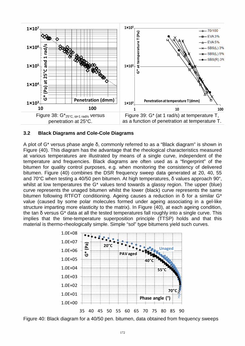
3.1 Equivalent Fraass Temperature and Equivalent Ring & Ball Temperature for Polymer Modified Bitumens Molenaar et al. (2004), found that the following equation, which represented more than 130 different bitumens (including elastomer and plastomer modified binders), describes the relation between G*25°C,ω=1 rad/s and pen25°C very well with minimal scatter (see also Figure 38): Log G*25°C,ω=1 rad/s = 7.845 – 1.642 (log pen25°C) ...(22) As the Fraass temperature is defined as TFraass = Tpen=1dmm, by substituting the value of 1dmm into equation (22) yields G* = 70 MPa. Using a similar argument, the softening point temperature (Ring & Ball) is defined by TRB = Tpen=800dmm, and by substitution of 800dmm into equation (22) a G* value of 1200 Pa is obtained. Thus is it possible to redefine the Fraass temperature and the Softening Point Temperature of unmodified and polymer modified bitumens. With the aid of DSR tests, the aforementioned two definitions allow the characterisation (and specification) of polymer modified bitumens in an analogous manner to the characterisation (and specification) of penetration grade unmodified bitumens. Furthermore, Molenaar et al. (2004) investigated the relationship between the standard penetration test at a range of test temperatures and G* at 1 rad/s for 3 types of polymer modified bitumens plus a base bitumen. The tests were conducted at 5°C, 10°C, 15°C, 20°C, and 25°C. The base bitumen used was a 70/100 pen, whilst the blended polymers were an EVA, a linear SBS and a radial SBS (at 3%, 5%, and 7% by mass). Figure (39) shows an example of the linear relationship on a log-log scale and indicates that using the 5 test temperatures listed earlier, each binder can be characterised by a (G*T,ω=1rad/s v.s. penT) relationship that is specific for the particular binder. It was proposed that this relationship be adopted as a basis for the continued use of the penetration test for polymer modified bitumens for practical purposes, e.g. delivery and production control.

171

1××××103

1××××104

1××××105

1××××106

1××××107

10 100

Penetration (dmm)G*

(P

a)

at

25

°C a

nd

1 r

ad

/s

Penetration at temperature T (dmm)

G*

at

tem

pe

ratu

re T

(P

a)

1 10 100

1××××105

1××××105

1××××105

Figure 38: G*25°C, ω=1 rad/s versus penetration at 25°C.

Figure 39: G* (at 1 rad/s) at temperature T, as a function of penetration at temperature T.

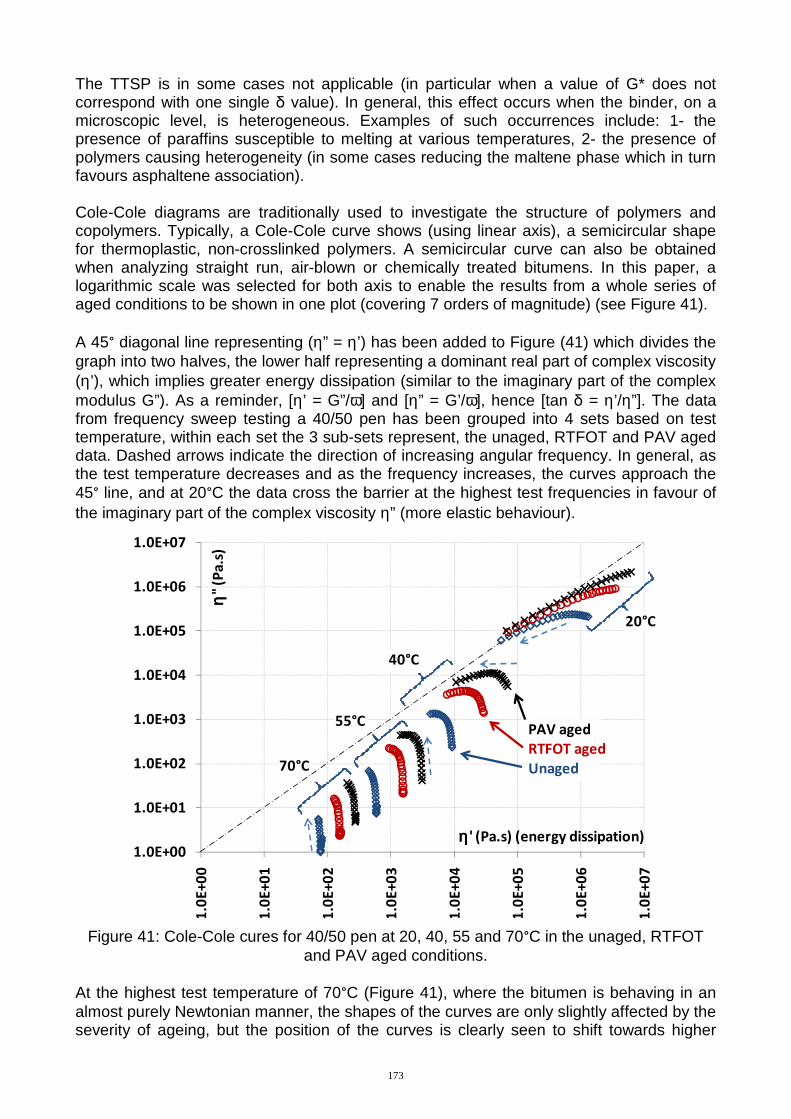
3.2 Black Diagrams and Cole-Cole Diagrams A plot of G* versus phase angle δ, commonly referred to as a “Black diagram” is shown in Figure (40). This diagram has the advantage that the rheological characteristics measured at various temperatures are illustrated by means of a single curve, independent of the temperature and frequencies. Black diagrams are often used as a “fingerprint” of the bitumen for quality control purposes, e.g. when monitoring the consistency of delivered bitumen. Figure (40) combines the DSR frequency sweep data generated at 20, 40, 55 and 70°C when testing a 40/50 pen bitumen. At high temperatures, δ values approach 90°, whilst at low temperatures the G* values tend towards a glassy region. The upper (blue) curve represents the unaged bitumen whilst the lower (black) curve represents the same bitumen following RTFOT conditioning. Ageing causes a reduction in δ for a similar G* value (caused by some polar molecules formed under ageing associating in a gel-like structure imparting more elasticity to the matrix). In Figure (40), at each ageing condition, the tan δ versus G* data at all the tested temperatures fall roughly into a single curve. This implies that the time-temperature superposition principle (TTSP) holds and that this material is thermo-rheologically simple. Simple “sol” type bitumens yield such curves.

1.0E+00

1.0E+01

1.0E+02

1.0E+03

1.0E+04

1.0E+05

1.0E+06

1.0E+07

1.0E+08

35 40 45 50 55 60 65 70 75 80 85 90

G*

(P

a)

Phase angle (°)

20°C

40°C

55°C

70°C

PAV aged

Unaged

Figure 40: Black diagram for a 40/50 pen. bitumen, data obtained from frequency sweeps

172

The TTSP is in some cases not applicable (in particular when a value of G* does not correspond with one single δ value). In general, this effect occurs when the binder, on a microscopic level, is heterogeneous. Examples of such occurrences include: 1- the presence of paraffins susceptible to melting at various temperatures, 2- the presence of polymers causing heterogeneity (in some cases reducing the maltene phase which in turn favours asphaltene association). Cole-Cole diagrams are traditionally used to investigate the structure of polymers and copolymers. Typically, a Cole-Cole curve shows (using linear axis), a semicircular shape for thermoplastic, non-crosslinked polymers. A semicircular curve can also be obtained when analyzing straight run, air-blown or chemically treated bitumens. In this paper, a logarithmic scale was selected for both axis to enable the results from a whole series of aged conditions to be shown in one plot (covering 7 orders of magnitude) (see Figure 41). A 45° diagonal line representing (η” = η’) has been added to Figure (41) which divides the graph into two halves, the lower half representing a dominant real part of complex viscosity (η’), which implies greater energy dissipation (similar to the imaginary part of the complex modulus G”). As a reminder, [η’ = G”/ω] and [η” = G’/ω], hence [tan δ = η’/η”]. The data from frequency sweep testing a 40/50 pen has been grouped into 4 sets based on test temperature, within each set the 3 sub-sets represent, the unaged, RTFOT and PAV aged data. Dashed arrows indicate the direction of increasing angular frequency. In general, as the test temperature decreases and as the frequency increases, the curves approach the 45° line, and at 20°C the data cross the barrier at the highest test frequencies in favour of the imaginary part of the complex viscosity η” (more elastic behaviour).

1.0E+00

1.0E+01

1.0E+02

1.0E+03

1.0E+04

1.0E+05

1.0E+06

1.0E+07

1.0

E+

00

1.0

E+

01

1.0

E+

02

1.0

E+

03

1.0

E+

04

1.0

E+

05

1.0

E+

06

1.0

E+

07

ηη ηη"

(Pa

.s)

ηηηη' (Pa.s) (energy dissipation)

55°C

70°C

20°C

40°C

PAV aged

RTFOT aged

Unaged

Figure 41: Cole-Cole cures for 40/50 pen at 20, 40, 55 and 70°C in the unaged, RTFOT and PAV aged conditions.

At the highest test temperature of 70°C (Figure 41), where the bitumen is behaving in an almost purely Newtonian manner, the shapes of the curves are only slightly affected by the severity of ageing, but the position of the curves is clearly seen to shift towards higher

173

viscosities (in terms of both η’ and η”). At 70°C the shape of the curves indicates the almost total dominance of the real part of complex viscosity η’ on the viscoelastic response, whilst as the test temperature is reduced (and equally as the bitumen is oxidised) the curves gradually rotate, become more linear in shape and approach the 45° line. This straightening of the curves indicates colloidal shifting from sol to gel structures. In this paper, the use of Cole-Cole curves was not explored further as it was felt that Black diagram representations were a more powerful analytical tool.

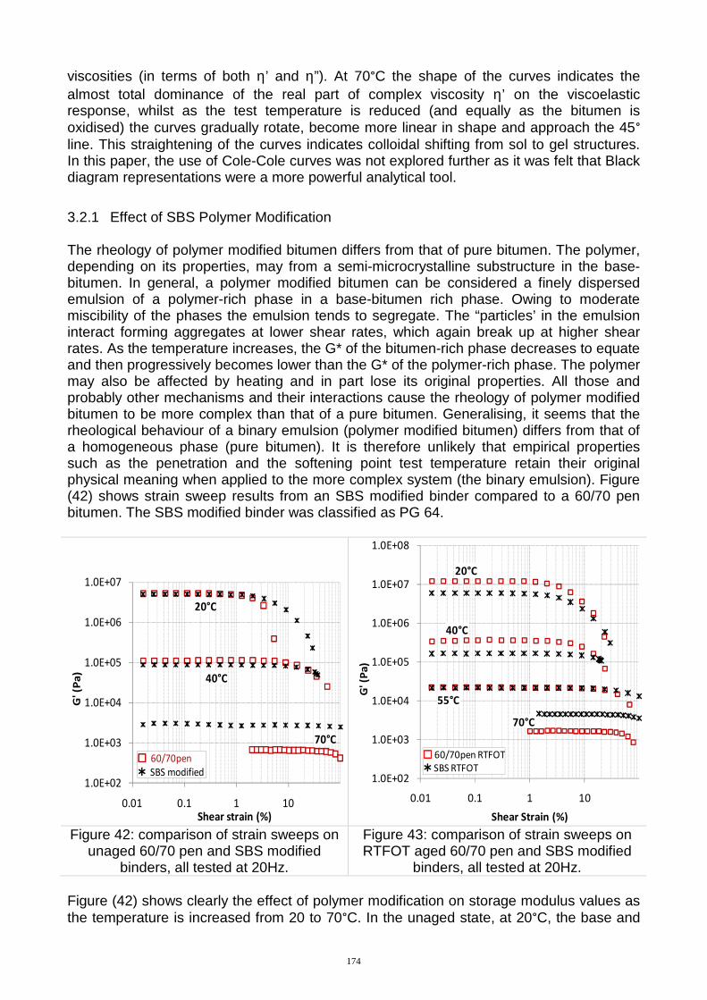
3.2.1 Effect of SBS Polymer Modification The rheology of polymer modified bitumen differs from that of pure bitumen. The polymer, depending on its properties, may from a semi-microcrystalline substructure in the base-bitumen. In general, a polymer modified bitumen can be considered a finely dispersed emulsion of a polymer-rich phase in a base-bitumen rich phase. Owing to moderate miscibility of the phases the emulsion tends to segregate. The “particles’ in the emulsion interact forming aggregates at lower shear rates, which again break up at higher shear rates. As the temperature increases, the G* of the bitumen-rich phase decreases to equate and then progressively becomes lower than the G* of the polymer-rich phase. The polymer may also be affected by heating and in part lose its original properties. All those and probably other mechanisms and their interactions cause the rheology of polymer modified bitumen to be more complex than that of a pure bitumen. Generalising, it seems that the rheological behaviour of a binary emulsion (polymer modified bitumen) differs from that of a homogeneous phase (pure bitumen). It is therefore unlikely that empirical properties such as the penetration and the softening point test temperature retain their original physical meaning when applied to the more complex system (the binary emulsion). Figure (42) shows strain sweep results from an SBS modified binder compared to a 60/70 pen bitumen. The SBS modified binder was classified as PG 64.

1.0E+02

1.0E+03

1.0E+04

1.0E+05

1.0E+06

1.0E+07

0.01 0.1 1 10

G' (P

a)

Shear strain (%)

20°C

70°C

40°C

���� 60/70pen

� SBS modified1.0E+02

1.0E+03

1.0E+04

1.0E+05

1.0E+06

1.0E+07

1.0E+08

0.01 0.1 1 10

G' (P

a)

Shear Strain (%)

20°C

40°C

55°C

70°C

���� 60/70pen RTFOT

� SBS RTFOT

Figure 42: comparison of strain sweeps on unaged 60/70 pen and SBS modified

binders, all tested at 20Hz.

Figure 43: comparison of strain sweeps on RTFOT aged 60/70 pen and SBS modified

binders, all tested at 20Hz. Figure (42) shows clearly the effect of polymer modification on storage modulus values as the temperature is increased from 20 to 70°C. In the unaged state, at 20°C, the base and

174

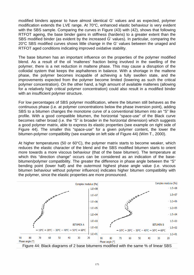
modified binders appear to have almost identical G’ values and as expected, polymer modification extends the LVE range. At 70°C, enhanced elastic behaviour is very evident with the SBS sample. Comparing the curves in Figure (43) with (42), shows that following RTFOT ageing, the base binder gains in stiffness (hardens) to a greater extent than the SBS modified binder (as evident by the increased G’ values). In particular, comparing the 20°C SBS modified curves shows little change in the G’ values between the unaged and RTFOT aged conditions indicating improved oxidative stability. The base bitumen has an important influence on the properties of the polymer modified blend. As a result of the oil ‘maltenes’ fraction being involved in the swelling of the polymer, there is a net reduction in maltene phase. This may cause a disruption of the colloidal system that keeps the asphaltenes in balance. With a shortage in the maltene phase, the polymer becomes incapable of achieving a fully swollen state, and the improvements expected from the polymer become limited (lowering as such the critical polymer concentration). On the other hand, a high amount of available maltenes (allowing for a relatively high critical polymer concentration) could also result in a modified binder with an insufficient polymer structure. For low percentages of SBS polymer modification, where the bitumen still behaves as the continuous phase (i.e. at polymer concentrations below the phase inversion point), adding SBS to a bitumen changes the monotone curve of a conventional bitumen into an “S” like profile. With a good compatible bitumen, the horizontal “space-use” of the Black curve becomes rather broad (i.e. the “S” is broader in the horizontal dimension) which suggests a good polymer matrix, able to express its elastic properties (see example on right side of Figure 44). The smaller this “space-use” for a given polymer content, the lower the bitumen-polymer compatibility (see example on left side of Figure 44) (Wim T., 2000). At higher temperatures (50 or 60°C), the polymer matrix starts to become weaker, which reduces the elastic character of the blend and the SBS modified bitumen starts to orient more towards a more viscous behaviour (that of the base bitumen). The temperature at which this “direction change” occurs can be considered as an indication of the base-bitumen/polymer compatibility. The greater the difference in phase angle between the “S” bending point (lower half) and the outermost highest phase angle value (i.e. viscous bitumen behaviour without polymer influence) indicates higher bitumen compatibility with the polymer, since the elastic properties are more pronounced.

Figure 44: Black diagrams of 2 base bitumens modified with the same % of linear SBS

175

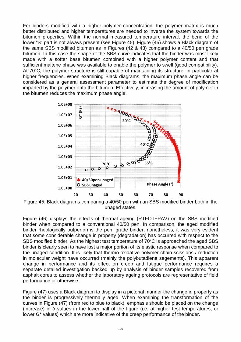
For binders modified with a higher polymer concentration, the polymer matrix is much better distributed and higher temperatures are needed to inverse the system towards the bitumen properties. Within the normal measured temperature interval, the bend of the lower “S” part is not always present (see Figure 45). Figure (45) shows a Black diagram of the same SBS modified bitumen as in Figures (42 & 43) compared to a 40/50 pen grade bitumen. In this case the shape of the SBS curve indicates that the binder was most likely made with a softer base bitumen combined with a higher polymer content and that sufficient maltene phase was available to enable the polymer to swell (good compatibility). At 70°C, the polymer structure is still capable of maintaining its structure, in particular at higher frequencies. When examining Black diagrams, the maximum phase angle can be considered as a general assessment parameter to estimate the degree of modification imparted by the polymer onto the bitumen. Effectively, increasing the amount of polymer in the bitumen reduces the maximum phase angle.

1.0E+00

1.0E+01

1.0E+02

1.0E+03

1.0E+04

1.0E+05

1.0E+06

1.0E+07

1.0E+08

20 30 40 50 60 70 80 90

G*

(P

a)

Phase Angle (°)���� 40/50pen unaged

���� SBS unaged

���� 40/50pen unaged

���� SBS unaged

���� 40/50pen unaged

���� SBS unaged

���� 40/50pen unaged

���� SBS unaged

20°C

40°C

55°C70°C

Figure 45: Black diagrams comparing a 40/50 pen with an SBS modified binder both in the

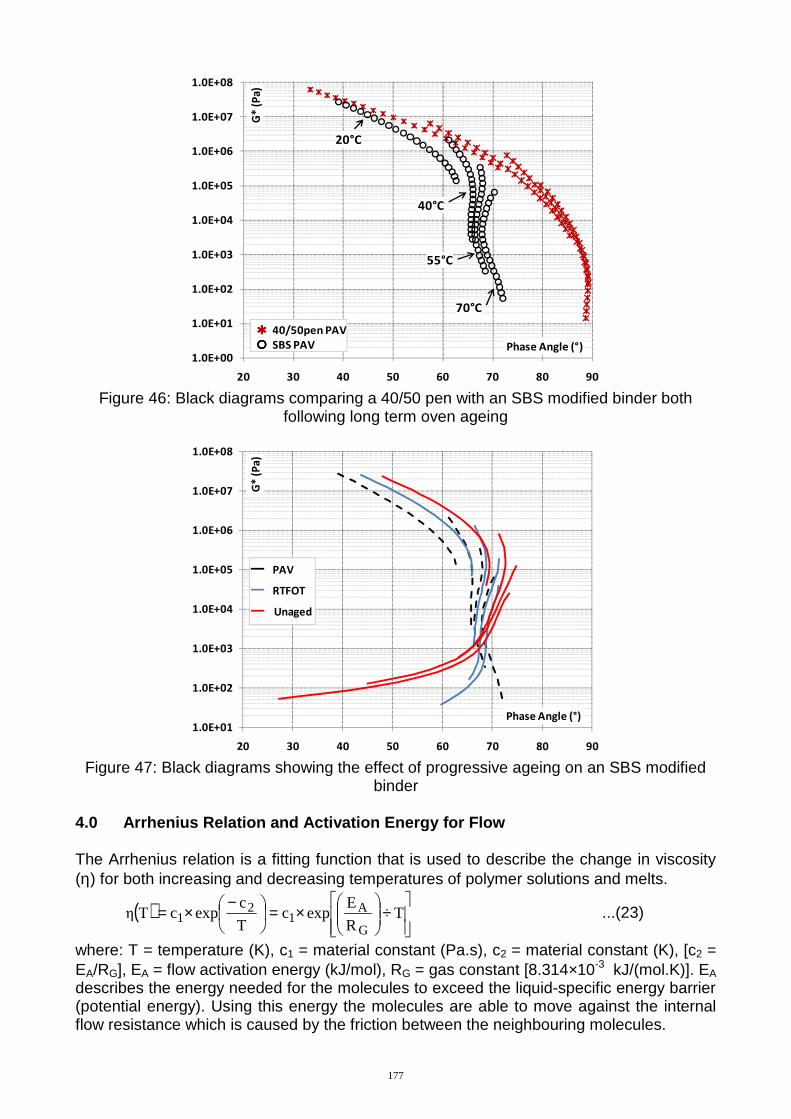
unaged states. Figure (46) displays the effects of thermal ageing (RTFOT+PAV) on the SBS modified binder when compared to a conventional 40/50 pen. In comparison, the aged modified binder rheologically outperforms the pen. grade binder, nonetheless, it was very evident that some considerable change in property (degradation) has occurred with respect to the SBS modified binder. As the highest test temperature of 70°C is approached the aged SBS binder is clearly seen to have lost a major portion of its elastic response when compared to the unaged condition. It is likely that thermo-oxidative polymer chain scissions / reduction in molecular weight have occurred (mainly the polybutadiene segements). This apparent change in performance and its effect on creep and fatigue performance requires a separate detailed investigation backed up by analysis of binder samples recovered from asphalt cores to assess whether the laboratory ageing protocols are representative of field performance or otherwise. Figure (47) uses a Black diagram to display in a pictorial manner the change in property as the binder is progressively thermally aged. When examining the transformation of the curves in Figure (47) (from red to blue to black), emphasis should be placed on the change (increase) in δ values in the lower half of the figure (i.e. at higher test temperatures, or lower G* values) which are more indicative of the creep performance of the binder.

176

1.0E+00

1.0E+01

1.0E+02

1.0E+03

1.0E+04

1.0E+05

1.0E+06

1.0E+07

1.0E+08

20 30 40 50 60 70 80 90

G*

(P

a)

Phase Angle (°)

���� 40/50pen PAV

���� SBS PAV

20°C

40°C

55°C

70°C

Figure 46: Black diagrams comparing a 40/50 pen with an SBS modified binder both

following long term oven ageing

1.0E+01

1.0E+02

1.0E+03

1.0E+04

1.0E+05

1.0E+06

1.0E+07

1.0E+08

20 30 40 50 60 70 80 90

G*

(P

a)

Phase Angle (°)

― PAV

― RTFOT

― Unaged

Figure 47: Black diagrams showing the effect of progressive ageing on an SBS modified

binder 4.0 Arrhenius Relation and Activation Energy for Flow The Arrhenius relation is a fitting function that is used to describe the change in viscosity (η) for both increasing and decreasing temperatures of polymer solutions and melts.

( )

÷

×=

−×= T

R

Eexpc

T

cexpcTη

G

A1

21 ...(23)

where: T = temperature (K), c1 = material constant (Pa.s), c2 = material constant (K), [c2 = EA/RG], EA = flow activation energy (kJ/mol), RG = gas constant [8.314×10-3 kJ/(mol.K)]. EA describes the energy needed for the molecules to exceed the liquid-specific energy barrier (potential energy). Using this energy the molecules are able to move against the internal flow resistance which is caused by the friction between the neighbouring molecules.

177

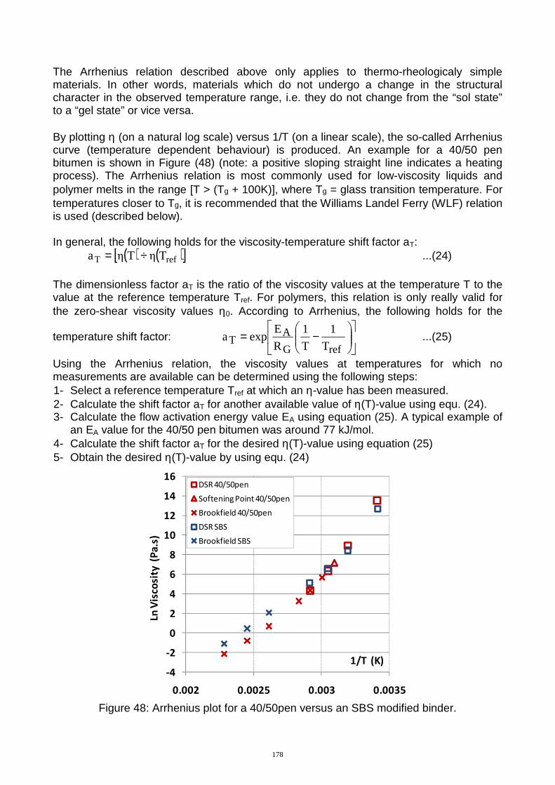
The Arrhenius relation described above only applies to thermo-rheologicaly simple materials. In other words, materials which do not undergo a change in the structural character in the observed temperature range, i.e. they do not change from the “sol state” to a “gel state” or vice versa. By plotting η (on a natural log scale) versus 1/T (on a linear scale), the so-called Arrhenius curve (temperature dependent behaviour) is produced. An example for a 40/50 pen bitumen is shown in Figure (48) (note: a positive sloping straight line indicates a heating process). The Arrhenius relation is most commonly used for low-viscosity liquids and polymer melts in the range [T > (Tg + 100K)], where Tg = glass transition temperature. For temperatures closer to Tg, it is recommended that the Williams Landel Ferry (WLF) relation is used (described below). In general, the following holds for the viscosity-temperature shift factor aT:

( ) ( )[ ]refT TηTηa ÷= ...(24) The dimensionless factor aT is the ratio of the viscosity values at the temperature T to the value at the reference temperature Tref. For polymers, this relation is only really valid for the zero-shear viscosity values η0. According to Arrhenius, the following holds for the

temperature shift factor:

−=

refG

AT T

1

T

1

R

Eexpa ...(25)

Using the Arrhenius relation, the viscosity values at temperatures for which no measurements are available can be determined using the following steps: 1- Select a reference temperature Tref at which an η-value has been measured. 2- Calculate the shift factor aT for another available value of η(T)-value using equ. (24). 3- Calculate the flow activation energy value EA using equation (25). A typical example of

an EA value for the 40/50 pen bitumen was around 77 kJ/mol. 4- Calculate the shift factor aT for the desired η(T)-value using equation (25) 5- Obtain the desired η(T)-value by using equ. (24)

-4

-2

0

2

4

6

8

10

12

14

16

0.002 0.0025 0.003 0.0035

Ln V

isco

sity

(P

a.s

)

1/T (K)

DSR 40/50pen

Softening Point 40/50pen

Brookfield 40/50pen

DSR SBS

Brookfield SBS

Figure 48: Arrhenius plot for a 40/50pen versus an SBS modified binder.

178

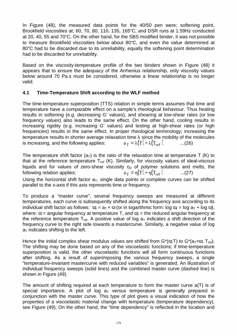
In Figure (48), the measured data points for the 40/50 pen were; softening point, Brookfield viscosities at; 60, 70, 80, 110, 135, 165°C, and DSR runs at 1.59Hz conducted at 20, 40, 55 and 70°C. On the other hand, for the SBS modified binder, it was not possible to measure Brookfield viscosities below about 80°C, and even the value determined at 80°C had to be discarded due to its unreliability, equally the softening point determination had to be discarded for unreliability. Based on the viscosity-temperature profile of the two binders shown in Figure (48) it appears that to ensure the adequacy of the Arrhenius relationship, only viscosity values below around 70 Pa.s must be considered, otherwise a linear relationship is no longer valid. 4.1 Time-Temperature Shift according to the WLF method The time-temperature superposition (TTS) relation in simple terms assumes that time and temperature have a comparable effect on a sample’s rheological behaviour. Thus heating results in softening (e.g. decreasing G’ values), and shearing at low-shear rates (or low frequency values) also leads to the same effect. On the other hand, cooling results in increasing rigidity (e.g. increasing G’ values) and testing at high-shear rates (or high frequencies) results in the same effect. In proper rheological terminology; increasing the temperature results in shorter average relaxation time λ since the mobility of the molecules is increasing, and the following applies: ( ) ( )refT TλTλa ÷= ...(26) The temperature shift factor (aT) is the ratio of the relaxation time at temperature T (K) to that at the reference temperature Tref (K). Similarly, for viscosity values of ideal-viscous liquids and for values of zero-shear viscosity η0 of polymer solutions and melts, the following relation applies: ( ) ( )refT TηTηa ÷= ...(27) Using the horizontal shift factor aT, single data points or complete curves can be shifted parallel to the x-axis if this axis represents time or frequency. To produce a “master curve”, several frequency sweeps are measured at different temperatures, each curve is subsequently shifted along the frequency axis according to its individual shift factor as follows: ωr = aT × ω (or in logarithmic form: log ωr = log aT + log ω), where: ω = angular frequency at temperature T, and ωr = the reduced angular frequency at the reference temperature Tref. A positive value of log aT indicates a shift direction of the frequency curve to the right side towards a mastercurve. Similarly, a negative value of log aT indicates shifting to the left. Hence the initial complex shear modulus values are shifted from G*(ω,T) to G*(aT×ω, Tref). The shifting may be done based on any of the viscoelastic functions; if time-temperature superposition is valid, the other viscoelastic functions will all form continuous functions after shifting. As a result of superimposing the various frequency sweeps, a single “temperature-invariant mastercurve with reduced variables” is generated. An illustration of individual frequency sweeps (solid lines) and the combined master curve (dashed line) is shown in Figure (49). The amount of shifting required at each temperature to form the master curve a(T) is of special importance. A plot of log aT versus temperature is generally prepared in conjunction with the master curve. This type of plot gives a visual indication of how the properties of a viscoelastic material change with temperature (temperature dependency), see Figure (49). On the other hand, the “time dependency” is reflected in the location and

179

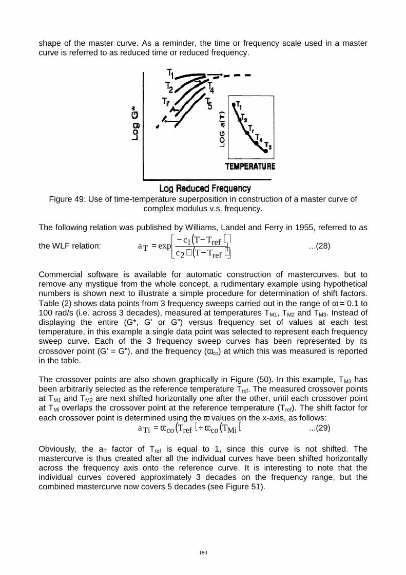
shape of the master curve. As a reminder, the time or frequency scale used in a master curve is referred to as reduced time or reduced frequency.

Figure 49: Use of time-temperature superposition in construction of a master curve of

complex modulus v.s. frequency. The following relation was published by Williams, Landel and Ferry in 1955, referred to as

the WLF relation: ( )( )

−+−−

=ref2

ref1T TTc

TTcexpa ...(28)

Commercial software is available for automatic construction of mastercurves, but to remove any mystique from the whole concept, a rudimentary example using hypothetical numbers is shown next to illustrate a simple procedure for determination of shift factors. Table (2) shows data points from 3 frequency sweeps carried out in the range of ω = 0.1 to 100 rad/s (i.e. across 3 decades), measured at temperatures TM1, TM2 and TM3. Instead of displaying the entire (G*, G’ or G”) versus frequency set of values at each test temperature, in this example a single data point was selected to represent each frequency sweep curve. Each of the 3 frequency sweep curves has been represented by its crossover point (G’ = G”), and the frequency (ωco) at which this was measured is reported in the table. The crossover points are also shown graphically in Figure (50). In this example, TM3 has been arbitrarily selected as the reference temperature Tref. The measured crossover points at TM1 and TM2 are next shifted horizontally one after the other, until each crossover point at TMi overlaps the crossover point at the reference temperature (Tref). The shift factor for each crossover point is determined using the ω values on the x-axis, as follows: ( ) ( )MicorefcoTi TTa ω÷ω= ...(29) Obviously, the aT factor of Tref is equal to 1, since this curve is not shifted. The mastercurve is thus created after all the individual curves have been shifted horizontally across the frequency axis onto the reference curve. It is interesting to note that the individual curves covered approximately 3 decades on the frequency range, but the combined mastercurve now covers 5 decades (see Figure 51).

180

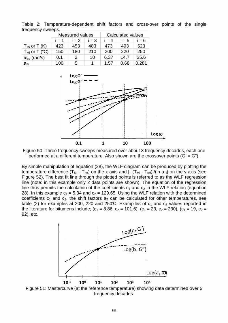
Table 2: Temperature-dependent shift factors and cross-over points of the single frequency sweeps. Measured values Calculated values

i = 1 i = 2 i = 3 i = 4 i = 5 i = 6 TMi or T (K) 423 453 483 473 493 523 TMi or T (°C) 150 180 210 200 220 250 ωco (rad/s) 0.1 2 10 6.37 14.7 35.6 aTi 100 5 1 1.57 0.68 0.281

Log ωωωω

1001010.1

Log G’

Log G”

Figure 50: Three frequency sweeps measured over about 3 frequency decades, each one

performed at a different temperature. Also shown are the crossover points (G’ = G”). By simple manipulation of equation (28), the WLF diagram can be produced by plotting the temperature difference (TMi - Tref) on the x-axis and [- (TMi - Tref)]/(ln aTi) on the y-axis (see Figure 52). The best fit line through the plotted points is referred to as the WLF regression line (note: in this example only 2 data points are shown). The equation of the regression line thus permits the calculation of the coefficients c1 and c2 in the WLF relation (equation 28). In this example c1 = 5.34 and c2 = 129.65. Using the WLF relation with the determined coefficients c1 and c2, the shift factors aT can be calculated for other temperatures, see table (2) for examples at 200, 220 and 250°C. Examp les of c1 and c2 values reported in the literature for bitumens include; (c1 = 8.86, c2 = 101.6), (c1 = 23, c2 = 230), (c1 = 19, c2 = 92), etc.

Log(bT.G”)

Log(aT.ω)

10-1 100 101 102 103 104

Figure 51: Mastercurve (at the reference temperature) showing data determined over 5 frequency decades.

181

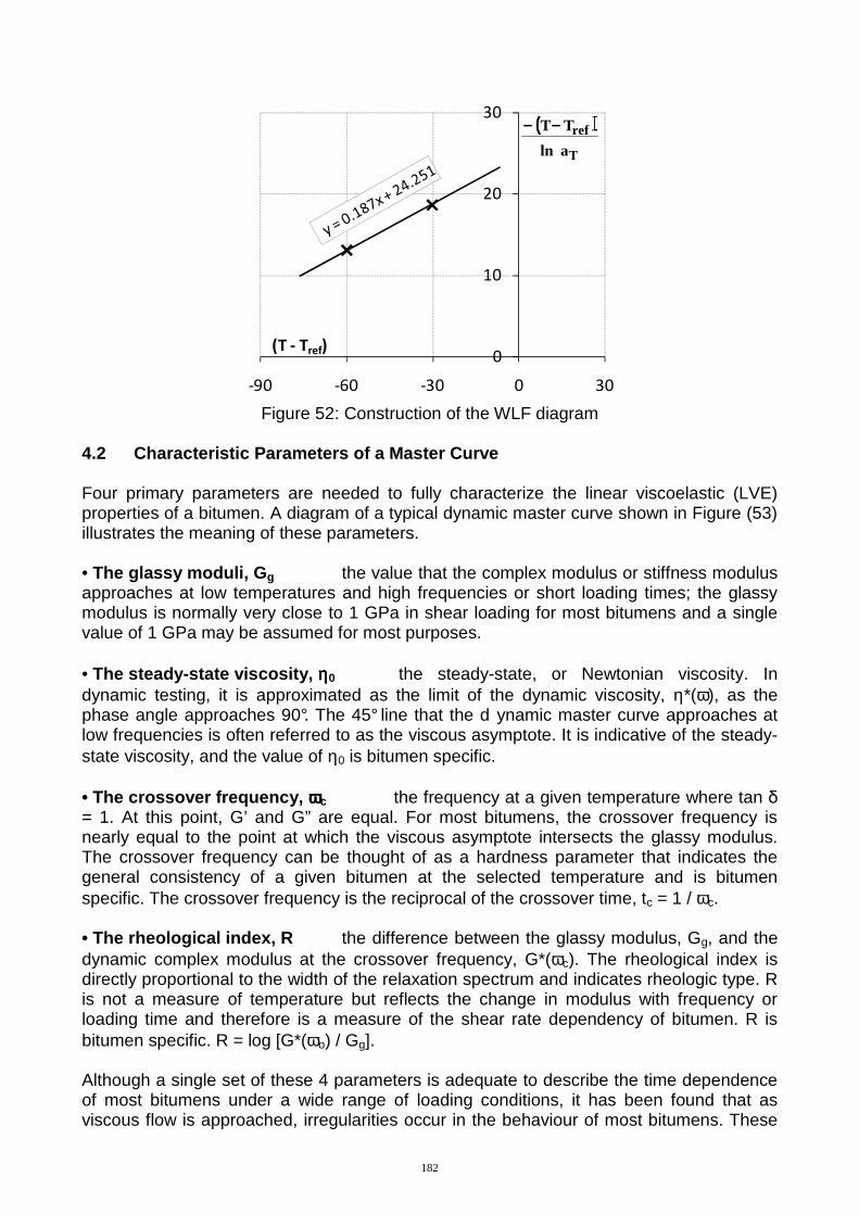
0

10

20

30

-90 -60 -30 0 30

(T - Tref)

(((( ))))T

ref

aln

TT−−−−−−−−

Figure 52: Construction of the WLF diagram

4.2 Characteristic Parameters of a Master Curve Four primary parameters are needed to fully characterize the linear viscoelastic (LVE) properties of a bitumen. A diagram of a typical dynamic master curve shown in Figure (53) illustrates the meaning of these parameters. • The glassy moduli, G g the value that the complex modulus or stiffness modulus approaches at low temperatures and high frequencies or short loading times; the glassy modulus is normally very close to 1 GPa in shear loading for most bitumens and a single value of 1 GPa may be assumed for most purposes. • The steady-state viscosity, ηηηη0 the steady-state, or Newtonian viscosity. In dynamic testing, it is approximated as the limit of the dynamic viscosity, η*(ω), as the phase angle approaches 90°. The 45° line that the d ynamic master curve approaches at low frequencies is often referred to as the viscous asymptote. It is indicative of the steady-state viscosity, and the value of η0 is bitumen specific. • The crossover frequency, ωωωωc the frequency at a given temperature where tan δ = 1. At this point, G’ and G” are equal. For most bitumens, the crossover frequency is nearly equal to the point at which the viscous asymptote intersects the glassy modulus. The crossover frequency can be thought of as a hardness parameter that indicates the general consistency of a given bitumen at the selected temperature and is bitumen specific. The crossover frequency is the reciprocal of the crossover time, tc = 1 / ωc. • The rheological index, R the difference between the glassy modulus, Gg, and the dynamic complex modulus at the crossover frequency, G*(ωc). The rheological index is directly proportional to the width of the relaxation spectrum and indicates rheologic type. R is not a measure of temperature but reflects the change in modulus with frequency or loading time and therefore is a measure of the shear rate dependency of bitumen. R is bitumen specific. R = log [G*(ωo) / Gg]. Although a single set of these 4 parameters is adequate to describe the time dependence of most bitumens under a wide range of loading conditions, it has been found that as viscous flow is approached, irregularities occur in the behaviour of most bitumens. These

182

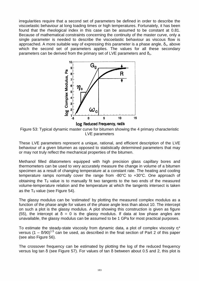
irregularities require that a second set of parameters be defined in order to describe the viscoelastic behaviour at long loading times or high temperatures. Fortunately, it has been found that the rheological index in this case can be assumed to be constant at 0.81. Because of mathematical constraints concerning the continuity of the master curve, only a single parameter is needed to describe the viscoelastic behaviour as viscous flow is approached. A more suitable way of expressing this parameter is a phase angle, δv, above which the second set of parameters applies. The values for all these secondary parameters can be derived from the primary set of LVE parameters and δv.

log

log

Figure 53: Typical dynamic master curve for bitumen showing the 4 primary characteristic

LVE parameters These LVE parameters represent a unique, rational, and efficient description of the LVE behaviour of a given bitumen as opposed to statistically determined parameters that may or may not truly reflect the mechanical properties of the bitumen. Methanol filled dilatometers equipped with high precision glass capillary bores and thermometers can be used to very accurately measure the change in volume of a bitumen specimen as a result of changing temperature at a constant rate. The heating and cooling temperature ramps normally cover the range from -80°C to +30°C. One approach of obtaining the Tg value is to manually fit two tangents to the two ends of the measured volume-temperature relation and the temperature at which the tangents intersect is taken as the Tg value (see Figure 54). The glassy modulus can be ‘estimated’ by plotting the measured complex modulus as a function of the phase angle for values of the phase angle less than about 10. The intercept on such a plot is the glassy modulus. A plot showing this construction is given as figure (55), the intercept at δ = 0 is the glassy modulus. If data at low phase angles are unavailable, the glassy modulus can be assumed to be 1 GPa for most practical purposes. To estimate the steady-state viscosity from dynamic data, a plot of complex viscosity η* versus (1 – δ/90)1.5 can be used, as described in the final section of Part 2 of this paper (see also Figure 56). The crossover frequency can be estimated by plotting the log of the reduced frequency versus log tan δ (see Figure 57). For values of tan δ between about 0.5 and 2, this plot is

183

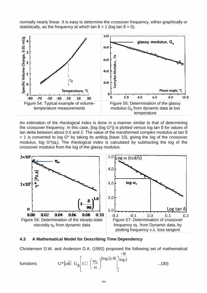
normally nearly linear. It is easy to determine the crossover frequency, either graphically or statistically, as the frequency at which tan δ = 1 (log tan δ = 0).

-90

2

1

0

-13010-10-30-50-70

3

4

Temperature, °CSp

eci

fic

Vo

lum

e C

ha

ng

e,

0.0

1 m

l/g

Tg

Figure 54: Typical example of volume-

temperature measurements Figure 55: Determination of the glassy modulus Gg from dynamic data at low

temperature An estimation of the rheological index is done in a manner similar to that of determining the crossover frequency. In this case, [log (log G*)] is plotted versus log tan δ for values of tan delta between about 0.5 and 2. The value of the transformed complex modulus at tan δ = 1 is converted to log G* by taking its antilog (base 10), giving the log of the crossover modulus, log G*(ωc). The rheological index is calculated by subtracting the log of the crossover modulus from the log of the glassy modulus.

Figure 56: Determination of the steady-state viscosity η0 from dynamic data

Figure 57: Determination of crossover frequency ωc from Dynamic data, by plotting frequency v.s. loss tangent

4.3 A Mathematical Model for Describing Time Dependency Christensen D.W. and Anderson D.A. (1992) proposed the following set of mathematical

functions: ( )2log

R/R2)(log

cg

ω

ω1GωG*

−

+= ...(30)

184

( )

+

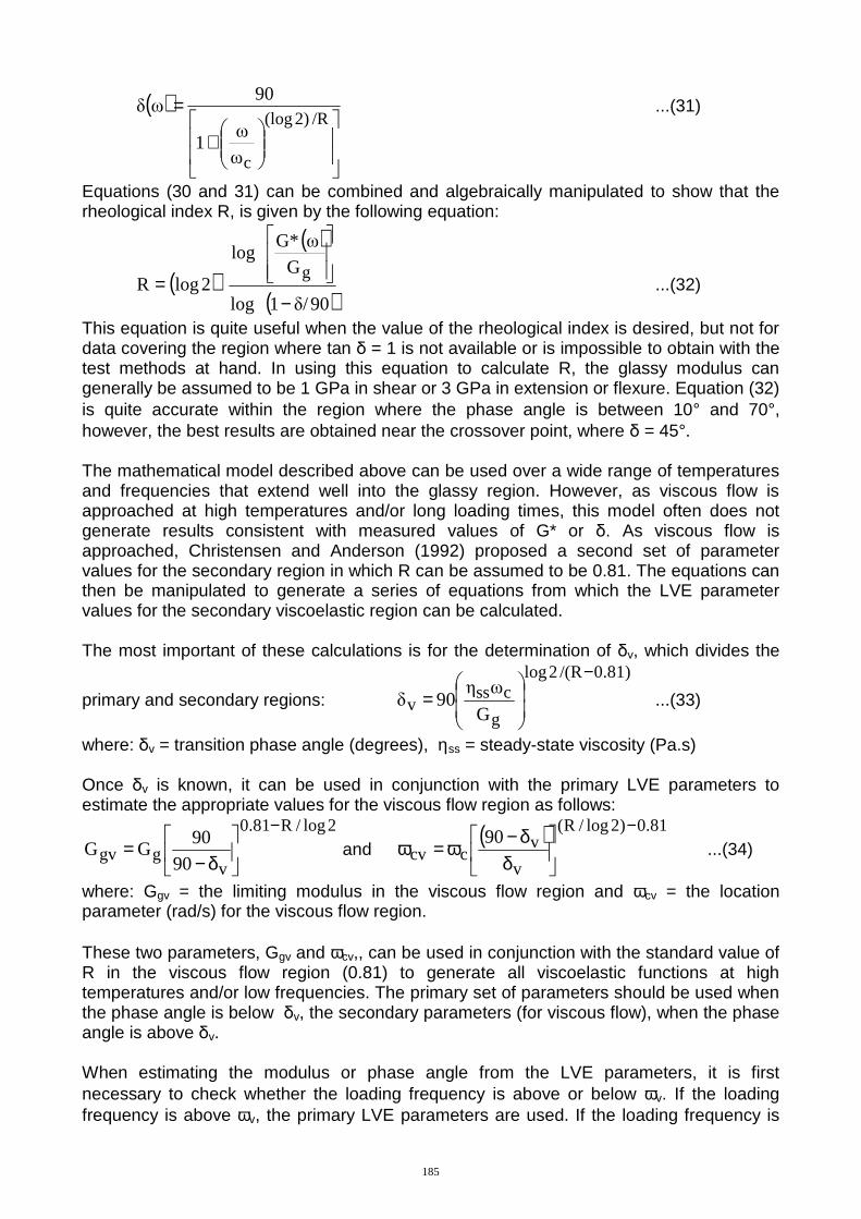
=/R2)(log

cω

ω1

90ωδ ...(31)

Equations (30 and 31) can be combined and algebraically manipulated to show that the rheological index R, is given by the following equation:

( )

( )

( )90δ/1log

G

ωG*log

2logRg

−

= ...(32)

This equation is quite useful when the value of the rheological index is desired, but not for data covering the region where tan δ = 1 is not available or is impossible to obtain with the test methods at hand. In using this equation to calculate R, the glassy modulus can generally be assumed to be 1 GPa in shear or 3 GPa in extension or flexure. Equation (32) is quite accurate within the region where the phase angle is between 10° and 70°, however, the best results are obtained near the crossover point, where δ = 45°. The mathematical model described above can be used over a wide range of temperatures and frequencies that extend well into the glassy region. However, as viscous flow is approached at high temperatures and/or long loading times, this model often does not generate results consistent with measured values of G* or δ. As viscous flow is approached, Christensen and Anderson (1992) proposed a second set of parameter values for the secondary region in which R can be assumed to be 0.81. The equations can then be manipulated to generate a series of equations from which the LVE parameter values for the secondary viscoelastic region can be calculated. The most important of these calculations is for the determination of δv, which divides the

primary and secondary regions:

0.81)/(R2log

g

cssv G

ωη90δ

−

= ...(33)

where: δv = transition phase angle (degrees), ηss = steady-state viscosity (Pa.s) Once δv is known, it can be used in conjunction with the primary LVE parameters to estimate the appropriate values for the viscous flow region as follows:

2log/R81.0

vggv 90

90GG

−

δ−= and

( ) 81.0)2log/R(

v

vccv

90−

δδ−ω=ω ...(34)

where: Ggv = the limiting modulus in the viscous flow region and ωcv = the location parameter (rad/s) for the viscous flow region. These two parameters, Ggv and ωcv,, can be used in conjunction with the standard value of R in the viscous flow region (0.81) to generate all viscoelastic functions at high temperatures and/or low frequencies. The primary set of parameters should be used when the phase angle is below δv, the secondary parameters (for viscous flow), when the phase angle is above δv. When estimating the modulus or phase angle from the LVE parameters, it is first necessary to check whether the loading frequency is above or below ωv. If the loading frequency is above ωv, the primary LVE parameters are used. If the loading frequency is

185

below ωv, the values for the viscous flow region are used. In practice, the primary parameters are of more interest and can be applied with confidence to temperatures up to about 45°C under typical traffic loading times. At higher temperatures, the only property that is of practical interest is the steady-state viscosity, which is one of the explicit parameters from the master curve. Therefore, in practical applications, it is generally not necessary to use the parameters for the viscous flow region. 5.0 Conclusions 1. The test temperature (T31) at which the penetration value is equivalent to 31dmm has been shown to lie half way between the Fraass freezing point and the softening point temperatures. By conducing the penetration test at a range of test temperatures and relating the result to the equi-penetrational T31 value, an enhanced graphical representation of penetration v.s. temperature relationship can be generated which is capable of displaying the results from bitumens having a range of temperature susceptibilities on one plot. 2. The effect of shear rate on the viscosity of bitumens has been described and the concept and importance of zero shear viscosity has been highlighted. 3. Dynamic shear rheometer test results were shown to fit in perfectly with other rheological characterisation tests, e.g. softening point and Brookfield rotational viscosity, but at the same time casting doubt over the accuracy of penetration-viscosity relations. 4. When conducting oscillatory tests using a dynamic shear rheometer, the 1st step prior to conducting any frequency sweeps is to determine the linear viscoelastic LVE limit at each test temperature. The LVE limits must be determined using the drop in storage modulus versus strain, or shear stress versus shear strain data. 5. G* approaches a limiting glassy modulus and the phase angle approaches 0° as the frequency is increased. 6. Shear stress and viscosity versus shear rate data both indicate that 40/50 pen bitumen is a Newtonian fluid at higher temperatures and shear thinning at lower ones. 7. Empirical relationships make it possible, based on the softening point value for an unmodified paving grade bitumen to be fully characterised with the US performance grading system. 8. Good relations have been reported in the literature between G*25°C,ω=1 rad/s and pen25°C for a large range of unmodified, elastomer and plastomer modified bitumens. 9. Black diagrams have the advantage that rheological characteristics measured at various temperatures can be combined into a single curve, irrespective of test temperature and frequencies. Black diagrams are often used as a “fingerprint” of a bitumen and are excellent tools to understand the behaviour of polymer modified bitumens. 10. The SBS modified binder tested in this investigation displayed superior elasticity compared to a conventional 40/50 pen, though more work needs to be carried out to understand the thermo-oxidative ageing effect on performance. 11. Time-temperature superposition can be applied using the Arrhenius and/or WLF relations, but these are primarily applicable for thermo-rheologicaly simple materials. At its most basic form, to fully characterise the linear viscoelastic properties of a bitumen from its dynamic stiffness mastercurve, the following parameters are required; the glassy modulus, the steady-state viscosity, the crossover frequency and finally the rheological index (difference between glassy modulus and modulus at crossover frequency).

186

References • Anderson D.A. et. al., Strategic Highway Research Program, SHRP-A-369, 1994,

Binder Characterization and Evaluation, Volume 3: Physical Characterization, Chapter 1: Linear Viscoelastic Model. ISBN 0-309-05767-1.

• Carswell J., Claxton M.J., Green P.J., 2000, “The classification of bitumens and polymer modified bitumens within the SHRP performance grading system”, 2nd Eurasphalt & Eurobitume Congress, Barcelona, Book 1, pp. 100-110.

• Christensen D.W. and Anderson D.A., 1992, “Interpretation of dynamic mechanical test data for paving grade asphalt cements”, AAPT Vol. 61, pp. 67-116.

• Garrick N.W., 1992, “Modelling the effects of temperature and shear rate on the viscosity of asphalt cements”, AAPT Vol. 61, pp. 1 to 28.

• Molenaar J.M.M., Hagos E.T. and Van De Ven M.F.C., 2004, “An investigation into the specification of rheological properties of polymer modified bitumen”, 3rd Eurasphalt & Eurobitume Congress, Vienna, Paper 203, Book 2, pp. 2080-2090.

• Mouillet V., Lapalu L., Planche J.P. and Durrieu F., 2004, “Rheological Analysis of Bitumens by Dynamic Shear Rheometer: Effect of the Thermal History on the Results”, 3rd Eurasphalt & Eurobitume Congress Vienna, paper 091.

• NCHRP 1-37A, 2004, Transport Research Board, Guide for Mechanistic-Empirical Design of New and Rehabilitated Pavement Structures, Part 2: Design Inputs, Chapter 2: Material Characterization.

• Páez Dueñas A., Gómez Saiz A., Bardesi Orúe-Echevarría A., 2004, “Rheological Measurements on some Spanish Bitumens. Correlations between Parameters”, 3rd Eurasphalt & Eurobitume Congress, Vienna, Paper 039, pp. 1679-1684.

• Petersen J.C. et. al., Strategic Highway Research Program, SHRP-A-370, 1994, Binder Characterization and Evaluation, Volume 4: Test Methods, Chapter 1: Dynamic Shear Rheometry. ISBN 0-309-05806-6.

• Wim T., 2000, “The Black Diagram, Only a Rheological Data Presentation ?” 2nd Eurasphalt & Eurobitume Congress, Book 1, pp. 862-872.

• Zolotarev V.A., Zintchenko V.N., Stolyarova L.V. and Pyrig Y.I., 2004, “Quantitative interrelation of softening point and brittleness temperature and penetration of road bitumens”, 3rd Eurasphalt & Eurobitumen Congress Vienna, paper 110, pp 1652-1658.

187