Investigating the relationship between petroleum product ...

STOCKHOLM SCHOOL OF ECONOMICS Department of Economics 659 Degree project in economics Spring 2015

Investigating the relationship between petroleum product subsidies and particulate matter concentrations: An empirical approach

Frida Lindqvist (22597) and Jorunn Ottesen (50147)

ABSTRACT: The aim of this paper is to examine how petroleum product consumer subsidies affect concentrations of the air-pollutant small particulate matter (PM10) through excessive consumption. An empirical cross-sectional approach is adopted to test the hypothesis that petroleum product subsidies increase concentrations of PM10. PM10 is known to cause adverse health effects and previous research show that fossil fuel subsidies are often inefficient and come with adverse economic, social and environmental consequences. Petroleum products, including gasoline, diesel and kerosene, are heavily subsidized. With international oil prices being low, now is a time of opportunity for petroleum product subsidy reform. The subsidization of petroleum products for consumers is not a problem limited to developing countries even though the issues differ in character and in terms of severity. The sample used in this study includes 100 countries, both developing and developed, in 2011. Due to issues of endogeneity in the model, instrumental variables are introduced for petroleum product consumer subsidies and per capita GDP. Our model yields approximately unbiased and consistent estimates. A coefficient of 0.3158 for the natural logarithm of petroleum product consumer subsidies is found to be statistically significant at a 1 % significance level. The practical significance can be discussed, since the model predicts an increase in PM10 concentrations by 0.3158 percentage units from a one percentage unit increase in the billion dollars spent on petroleum product consumer subsidies. However, no threshold of PM10 concentrations without adverse health effects has yet been identified.

Keywords: petroleum product consumer subsidies, fossil fuel subsidies, particulate matter, PM10, subsidy reform

JEL Classification: C21, C26

Supervisor: Martina Björkman Nyqvist Date submitted: 17th May 2015 Date examined: 11th June 2015 Discussant: Diana Landelius and Benjamin Dousa Examiner: Chloé Le Coq

2

Acknowledgments We are thankful for the assistance of our supervisor Martina Björkman Nyqvist, and Dr. Mark

Sanctuary for his comments and valuable guidance.

Furthermore, we would like to give a big thanks to each other.

3

Table of Contents

1. INTRODUCTION ....................................................................................................................................... 4

1.1 BACKGROUND ........................................................................................................................................................ 4

1.2 PREVIOUS RESEARCH .......................................................................................................................................... 8

1.2.1 ECONOMIC ASPECTS & EKC ........................................................................................................................... 12

1.3 PURPOSE .................................................................................................................................................................... 15

2. RESEARCH FOCUS ............................................................................................................................... 17

3. METHOD ................................................................................................................................................... 19

3.1 MODEL SPECIFICATION ......................................................................................................................................... 20

3.2.1 ADDRESSING ENDOGENEITY IN THE MODEL .............................................................................................. 22

4. DATA ........................................................................................................................................................... 26

4.1 DEPENDENT VARIABLE OF INTEREST ............................................................................................................... 26

4.2 INDEPENDENT VARIABLE OF INTEREST ........................................................................................................... 27

4.3 CONTROL VARIABLES ........................................................................................................................................... 29

4.4 DATA EXPLORATION AND TRANSFORMATION OF VARIABLES ................................................................ 30

5. RESULTS ................................................................................................................................................... 33

6. DISCUSSION ............................................................................................................................................. 37

7. CONCLUSION .......................................................................................................................................... 40

8. SUMMARY ................................................................................................................................................ 42

REFERENCES .............................................................................................................................................. 44

APPENDIX I .................................................................................................................................................. 52

APPENDIX II ................................................................................................................................................. 53

4

1. Introduction

1.1 Background

For decades fossil fuel subsidies have encouraged wasteful spending and harmful emissions.

They put a strain on national budgets and international efforts to combat climate change are

undermined. Except damaging effects on the environment through emissions and reducing

investment available for clean energy, fuel subsidies crowd-out public spending (i.e. on

health, education and infrastructure) and benefit mostly highly-income groups.1 2 In 2011, the

International Monetary Fund (IMF) estimates of pre-tax producer- and consumer subsidies

reached $480 billion, which reflects 0.7 % of global GDP. Adjusting for corrective taxation to

account for negative externalities of their consumption, the subsidy3 estimates amounted to

$1.9 trillion4. In comparison, the total sum of fossil fuel subsidies was more than four times

the sum invested in improving energy efficiency globally and over four times the value of

subsidies to renewable energy.5

Problems with energy subsidies arise in both developed and developing countries although the

underlying cause of the problem is somewhat different. In many developing countries,

consumer prices are directly controlled by governments, which results in the volatility of

1 Christopher Beaton et al., “Untold billions: fossil-fuel subsidies, their impacts and their path to reform”, IISD, (working paper, 21 April 2010), <https://www.iisd.org/gsi/sites/default/files/synthesis_ffs.pdf>, accessed 15 2 Christian Ebeke and Constant Lonkeng Ngouana, “Energy subsidies and public social spending: Theory and Evidence”, International Monetary Fund, (working Paper No. 15/101, May 2015) <http://www.imf.org/external/pubs/ft/wp/2015/wp15101.pdf>, accessed 15 April 2015. 3 The IMF defines post-tax subsidies as the sum of pre-tax and tax subsidies. Post-tax subsidies are four times larger than pre-tax subsidies, and advanced economies account for 40 % of post-tax subsidies. But post-tax subsidies as a share of gross domestic product are roughly eight times larger in the Middle East and North African regions than in developed countries. 4 Carlo Cottarelli, Antoinette M. Sayeh, and Masood Ahmed, “Energy Subsidy Reform: Lessons and Implications”, International Monetary Fund, (executive summary, 28 Jan. 2013) <http://www.imf.org/external/np/pp/eng/2013/012813.pdf>, accessed on 25 April 2015. 5 Dave Sawyer and Seton Stiebert, “Fossil Fuels - At What Cost? Government support for upstream oil activities in three Canadian provinces: Alberta, Saskatchewan, and Newfoundland and Labrador”, IISD, (working paper, Nov. 2010) <https://www.iisd.org/GSI/fossil-fuel-subsidies/fossil-fuels-what-cost>, accessed 28 April 2015.

5

domestic energy prices being reduced and affecting the state budget instead of the consumer.6

Governments in developed countries do not set fossil fuel prices and they subsidize fossil

fuels to a lesser extent by more sophisticated methods.7Apart from inducing fiscal costs for

governments another possible economic consequence of fossil fuel subsidies in developing

countries is the crowding out of public social spending.8 Although advanced economies have

mostly phased out generalized consumer fossil fuel subsidies that are frequent in the

developing world, other forms of subsidization and the under-taxation of fossil fuels in both

developing and developed countries is economically inefficient in the sense that it distorts

market signals, leading to inefficient resource allocation and a lower long-run economic

growth.9

Considering the many adverse effects of fossil fuel subsidies, one may wonder why they are

still in place. The main reasons concern their definition, polity, transparency and the

economy. A fossil fuel subsidy is generally defined as any government action that lowers the

cost of fossil fuel energy production, raises the price received by energy producers or lowers

the price paid by energy consumers.10 Fossil fuel subsidy programs especially targeted at the

poor fall under this classification and even engaged activists for fossil fuel subsidy reform

would probably not agree that all of those should be removed.11 The adverse effects versus

any possible benefits can vary a lot between subsidies even though they, by definition, fall in

the same category. However, subsidies designed to alleviate poverty frequently fail to meet

6 David Coady and Baoping Shang, “Energy Subsidies in Developing Countries: Treating the disease while symptoms abate”, VOX, (published article, 13 Jan. 2015) <http://www.voxeu.org/article/energy-subsidies-developing-countries>, accessed 20 April 2015. 7 Ambrus Bárány and Dalia Grigonytė, “Measuring Fossil Subsidies”, European Commission, (working paper, March 2015) <http://ec.europa.eu/economy_finance/publications/economic_briefs/2015/pdf/eb40_en.pdf>, accessed 23 April 2015. 8 Ebeke and Lonkeng Ngouana, “Theory and Evidence”. 9 Bárány and Grigonytė, “Measuring Fossil Subsidies”. 10 Laura Merrill, “Fossil-Fuel Subsidy Reform Mitigating emissions through getting the price right”, Global Subsidies Initiative, International Institute for Sustainable Development, (working paper, 2014) <https://www.iea.org/media/workshops/2014/cop20/Merrill.pdf>, accessed 23 April 2015. 11 Robert Rapier, “The surprising reason that oil subsidies persist: Even liberals love them”, Forbes, (published article, 25 April 2012) <http://www.forbes.com/sites/energysource/2012/04/25/the-surprising-reason-that-oil-subsidies-persist-even-liberals-love-them/>, accessed 23 April 2015.

6

that goal.12 Coady et al. show that there is substantial leakage of benefits from fossil fuel

subsidies to other income groups.13 14 On average, the richest 20 % of households in low- and

middle-income countries receive six times more in fuel subsidies than the poorest 20 %. In

spite of the observed progressivity of fuel subsidies, it is important to note that low-income

groups are vulnerable to the removal or decrease of such subsidies and reforms should be

carefully evaluated before executed.

The politics surrounding fossil fuel subsidies represent another important reason for their

persistence. Attempts of removal of the consumer subsidies often face political resistance. In

multiple occasions subsidy reforms have resulted in, sometimes violent, protests by the

public.15 Governments in resource-rich countries are subject to political pressure by the public

to share the country’s endowments with its inhabitants.

Regarding transparency, current overview of the magnitude of fossil fuels is insufficient. It is

necessary to develop an accurate image of the level and nature of global fossil fuel subsidies

in order to enable further and more valid research of their impacts and facilitate monitoring of

the development towards or away from de-subsidization.16 David Victor’s work on fossil fuel

subsidies, The Politics of Fossil Fuel Subsidies, points out the importance of transparency and

more public information and how this will help broaden public support and enable successful

subsidy reforms.

Due to the energy intensity in the process of industrialization and growth, many developing

countries see fossil fuel subsidies as a mean to encourage economic activity. Worry of

decreasing economic activity and a lowered GDP is another counter-argument for 12 Beaton et al., “Untold billions: fossil-fuel subsidies, their impacts and their path to reform”. 13 David Coady et al., “Petroleum product subsidies, costly, inequitable, and rising”, International Monetary Fund, (working paper, 25 Feb. 2010) <https://www.imf.org/external/pubs/ft/spn/2010/spn1005.pdf> accessed 5 May 2015. 14 Javier Arze del Granado, David Coady, and Robert Gillingham, “The unequal benefits of fuel subsidies: a review of evidence for developing countries”, International Monetary Fund, (working paper, Sep 2010) <http://www.imf.org/external/pubs/ft/wp/2010/wp10202.pdf>, accessed 15 April 2015. 15 Richard Anderson, “Fossil fuel subsidies growing despite concerns”, BBC, (electronic article, 29 April 2014) <http://www.bbc.com/news/business-27142377>, accessed 18 April 2015. 16 Beaton et al., “Untold billions: fossil-fuel subsidies, their impacts and their path to reform”.

7

governments to remove fossil fuel subsidies and a factor that further increases public

resistance. However, the research findings regarding the removal of fossil fuel subsidies and

its aggregate effects on GDP in OECD and non-OECD countries agree that the relationship is

positive. Even with those findings in mind, worry about decreases in GDP from subsidy

removal might not be unfounded. Some single country modelled and empirical analyses

indicate a slight short-term decline in economic output.17 The prioritizing of short-run

economic output, together with the definition aspect previously discussed, is probably the

most explanatory reasons subsidies are persistent in the developed countries as well as the

developing ones. A discussed topic in environmental economics is naturally the relationship

between environmental quality and economy. A frequently used hypothesis regarding this

relationship is that of the Environmental Kuznet’s curve which implications will be presented

and discussed in the literature review of this thesis.

A probable consequence of fossil fuel subsidies universal in all countries, irrespective of

development status, is air pollution and its effect on human health. As opposed to producer

subsidies, consumer subsidies encourage excessive consumption of energy. The current high

levels of fossil fuel consumer subsidies (in both absolute and relative terms) favour the use of

fossil fuels. Fossil fuel combustion is known to be a major contributor to air pollutants. In

recent years awareness about particulate matter as the component of air pollution that affects

more people than any other pollutant has reached consensus.18 There is a close relationship

between increased mortality and high exposure to concentrations of small particles

(particulate matter of 10 microns in diameter or less, denoted PM10). An increase of 10

µg/m3 in PM10 is estimated to increase daily mortality by 0.2 – 0.6 %.19 Particulate matter

also seems to be the air pollutant most closely related to increased cancer frequency,

17 Beaton et al., “Untold billions: fossil-fuel subsidies, their impacts and their path to reform”. 18 Regional Office for Europe Joint WHO/Convention Task Force on the Health Aspects of Air Pollution and World Health Organization, “Health risks of particulate matter from long-range transboundary air pollution”, World Health Organization, (working paper, 2006) <http://www.euro.who.int/__data/assets/pdf_file/0006/78657/E88189.pdf>, accessed 15 April 2015. 19 World Health Organization and Regional Office for Europe, “Health Aspects of Air Pollution with Particulate Matter, Ozone and Nitrogen Dioxide”, World Health Organization, (working paper, 15 Jan. 2003) <http://www.euro.who.int/__data/assets/pdf_file/0005/112199/E79097.pdf, accessed 15 April 2015.

8

especially lung cancer20 and exposures from human sources is expected to lower average life

expectancy by 8,6 months. In the European Union PM10 concentrations in most cities are in

line with the WHO Air Quality Guidelines of 20 µg/m3 as an annual mean of PM10.21 22 The

exposure in fast-developing countries are however often far higher than in developed

countries.

Outdoor air pollution was expected to cause 3,7 million premature deaths worldwide in 2012,

88 % of these occurred in low- and middle-income countries. It is estimated that deaths

related to air pollution can be cut by around 15 % if particulate matter (PM10) pollution is

reduced from 70 to 20 micrograms per cubic metre (µg/m).23

The International Monetary Fund (IMF) estimated that the petroleum product consumer

subsidies amounted to ca 50 % of total fossil fuel subsidies in 2011. Being the most heavily

subsidized fuel, we deem it to be of interest to assess the relationship between petroleum

product consumer subsidies and the level of PM10 concentrations in the air. Considering the

currently low oil prices, this is a time of opportunity for many countries to go through with

petroleum product subsidy reform. Gathering public support is easier than in times when the

immediate threat of high international oil prices being passed through, and fiscal costs are

lower. As the oil price increases the strains on the government budgets will tighten and the

public’s grip of their wallet might as well, decreasing the likelihood of success in attempted

reforms.24

1.2 Previous Research

One of few studies available that considers the impacts of product consumer subsidies on

PM10 is What are the effects of fossil fuel subsidies on growth, the environment and

20 World Health Organization and Regional Office for Europe, “Health Aspects of Air Pollution with Particulate Matter, Ozone and Nitrogen Dioxide”. 21 The European commission reports the somewhat higher 40 µg/m3 as a directive limit value for PM10. 22 World health organization, “Ambient (outdoor) air quality and health”, World Health Organization, (fact sheet, March 2014) < http://www.who.int/mediacentre/factsheets/fs313/en/>, accessed 3 April 2015. 23 WHO, “Ambient (outdoor) air quality and health”. 24 Coady and Shang, “Energy Subsidies in Developing Countries: Treating the disease while symptoms abate”.

9

inequality?.25 In relation to our paper, this one investigates if and how fossil fuel subsidies

cause negative environmental externalities. When the dependent variable is the natural

logarithm of PM10 the coefficients of gasoline- and diesel subsidies are positive and

significant at a 5 % significance level. The results indicate a 0.06 % increase in PM10

concentrations (µg/m) from a one dollar increase in per litre gasoline subsidy and a 0.05 %

increase in PM10 concentrations resulting from a one dollar increase in per litre diesel

subsidy. When using instrumental variables, only gasoline subsidies are significant (5 %) with

the coefficient being 0.1163. As in other studies considering the area of subsidies, some issues

regarding the subsidy estimates are commented on.26

Despite the evidence of potential severe health effects from PM10, scarce public resources in

developing countries have limited their monitoring of particulate matter. Thus, some

policymakers in developing countries remain uninformed about their residents exposure to

PM10. The study Air Pollution in World Cities (PM10) attempts to decrease this information

gap by predicting PM10 levels using the The Global Model of Ambient Particulates

(GMAPS), using data from the World Health Organization and other reliable sources. The

study find the main causes of PM10 to be the scale and structure of economic activity, the

energy mix, the strength of local pollution controls and geographic and atmospheric

conditions that affect pollutant dispersion in the atmosphere.27 Further, the United Nations

provides case studies of several countries in a report using local Air-Pollution modelling,

Global Climate Change Modelling and Natural Resource Depletion.28 The relationship

generally established between energy subsidies and PM10 is positive. Among others, the

countries included in the report are Iran, Chile and Indonesia. In the case study of Chile where

the particular relationship between petroleum product consumer subsidies and PM10 is

25 Christopher J. Holton, “What are the effects of fossil-fuel subsidies on growth, the environment, and inequality?”, MSc thesis (The University of Nottingham, 2012), p. 60. 26 Holton, “What are the effects of fossil-fuel subsidies on growth, the environment, and inequality?”. 27 David R. Wheeler et al., “Air pollution in world cities (PM10)”, The World Bank, (published paper, 2006) <http://econ.worldbank.org/WBSITE/EXTERNAL/EXTDEC/EXTRESEARCH/0,,contentMDK:20785646~pagePK:64214825~piPK:64214943~theSitePK:469382,00.html>, accessed 2 May 2015. 28 Igor Bashmakov et al., “Energy subsidies: lessons learned in assessing their impact and designing policy reforms”, The United Nations Foundation, (working paper, 2003) <http://www.unep.ch/etu/publications/energySubsidies/Energysubreport.pdf>, accessed 14 April 2015.

10

assessed, the findings indicate that when a direct subsidy is removed, the level of PM10

decreases with 4.7 % due to consumers switching to less polluting fuels.

In spite of the shortage of investigation of the particular relationship we are interested in,

research undertaken that is related to our research question can provide us with valuable

knowledge and a foundation on which to build our empirical model.

Transport has been deemed to be a large contributor to PM10 levels in the air due to fuel

combustion and coarse dust particles stirred up by vehicles on, in particular, paved roads 29

The Study on the Particulate Matter PM10 composition in the atmosphere of Chillán, Chile

measures the concentration of PM10 in urban sites of the city Chillán. It is concluded that the

urban traffic is the most essential source to the higher concentrations of PM10 in the

downtown areas.30 Their chemical analysis show that carbonaceous substances is one of the

most abundant components of PM10 together with crustal material.

Another study; Macroeconomic factors for sustainable growth: Analytical framework and

Policy Studies of Brazil and Chile, uses the ECOGEM model to analyze emission taxes on

PM10 which is shown to lead to reductions in the emissions of other pollutants as well. They

continue by investigating the impact of raising fuel taxes until a 10 % decrease in PM10

ug/m3 is reached. The authors find that an increase in fuel VAT and corporate taxes by 150 %

is needed to reduce PM10 levels by approximately 10 %. It should be noted that the

ECOGEM model has some data limitations that should be overcome in order to improve its

analytical capabilities. Nevertheless, these results indicate a rather inelastic demand for fossil

fuels. Related to our work, this implies that we should expect a low coefficient of petroleum

product consumer subsidies.

29 Dennis R. Fitz and Charles Bufalino, “Measurement of PM10 emission factors from paved roads using on-boards particle sensors”, MSc thesis (University of California, 2004), 18. 30 Jose E. Celis Hidalgo, “A study of the particulate matter PM10 composition in the atmosphere of Chillán, Chile”, Chemosphere, 02 (published work, 2004), <http://www.researchgate.net/publication/9038282_A_study_of_the_particulate_matter_PM10_composition_in_the_atmosphere_of_Chilln_Chile>, accessed 5 May 2015.

11

Since our study is of how petroleum product consumer subsidies affect PM10 levels through

the mechanism of increased petroleum product consumption, we are interested in research on

the price elasticity of demand of these products. A study summarizing price elasticities

suggest price elasticities to range between nearly zero and -0.25 (short-term) and between -

0.21 to -0.86 (long-term).31 Based on a review of 124 developed and developing countries, a

range of values are estimated for the demand price elasticity - between -0.11 and -0.33 for

gasoline, and between -0.13 and -0.38 for diesel. Long-run price elasticities are estimated to

be larger than those found for the short-term.32 For developed countries, mean price elasticity

for fuel consumption is found to be ranging from -0.25 (short run) to -0.64 (long run).33 Thus,

the demand for oil seems rather inelastic and very inelastic in the short-run which is intuitive.

Intuitive a priori reasoning predicts these elasticities to be low since there are few direct

substitutes for oil.34 Intuition can also explain why the short-term elasticities are lower than

the long-term elasticities and why country studies on- or including developing countries yield

larger price inelasticities. Mileage is typically likely to be more price-responsive in

developing countries.35

Various researchers have studied emissions of other air pollutants than PM10 and their

potential relationship with fossil fuel subsidy reform. Most of the research regards greenhouse

gases and C02 in particular. The Environmentally harmful subsidies: Barriers to sustainable

development by David Pearce concludes that the removal of fossil fuel subsidies would give

31 John C. B. Cooper, “Price elasticity of demand for crude oil: estimates for 23 countries”, Organization of the Petroleum Producing Countries, (published paper, March 2003) <http://15961.pbworks.com/f/Cooper.2003.OPECReview.PriceElasticityofDemandforCrudeOil.pdf>, accessed 10 May 2015. 32 Carol Dahl, “Measuring global gasoline and diesel price and income elasticities”, (working paper, Colorado School of Mines, 2012). 33 J. Dargay, M. Hanly and P. Goodwin, “Elasticities of road traffic and fuel consumption with respect to price and income: a review”, Transport Reviews, 24(3), 275-292 (published work, 2004), accessed 15 May 2015. 34 U.S. Energy Information Administration, “Oil crude and petroleum products”, U.S. Energy Information Administration, (electronic article, 21 April 2015) <http://www.eia.gov/energyexplained/index.cfm?page=oil_home>, accessed 25 April 2015. 35 J. Rogat, “The determinants of gasoline demand in some Latin American Countries”, (working paper, Technical University of Denmark, 2001).

12

results that far exceed what the Kyoto Protocol would deliver.36 Research on the subject of

fossil fuel combustion and its effects on air quality has been carried out by several influential

institutions. Estimates from the IEA’s 2010 World Energy Outlook indicate that an absolute

removal of fossil fuel consumption subsidies could reduce CO2 emissions by 5.8 % by 2020.

In a joint report from 2010 (IEA, OPEC, OECD and the World Bank) the global greenhouse

gas emissions was estimated to decrease by 10 % by 2050 if fossil fuel subsidies were phased

out. In 2013, using their own estimates of tax-inclusive subsidies, the IMF reported that

raising energy prices to levels eliminating these would reduce CO2 emission by 4.2 billion

tons and SO2 emissions by 10 million tons. A 13 % reduction in other local pollutants is also

predicted.37 These local pollutants are undefined in the report but can be assumed to include

PM10. The most recent estimation comes from a new report by the Nordic Council of

Ministers and the Global Subsidies Initiative released in february 2015.38 Using IEA subsidy

estimates their prediction is that the removal of fossil-fuel subsidies to consumers and to

society could reduce global greenhouse gas (GHG) emissions by between 6 - 13 % by 2050.

1.2.1 Economic aspects and the Environmental Kuznet’s Curve

Previous research has shed light on economic consequences of fossil fuel subsidies. With

significant variation in magnitude, a review of six modelling and empirical studies on the

effect of fossil fuel subsidy removal on GDP show that the studies yield similar results. The

results indicate that the effect of subsidy reform is positive in both OECD and non-OECD

countries. Broken down into blocks, the results for the two country groups were similar and

increasing.39 Findings of Burniaux et al uncover significant GDP or real-income declines in

some non-OECD countries. Some single country modelled and empirical analyses also

36 David Pearce, “Environmentally harmful subsidies: barriers to sustainable development”, (working paper, University College London and Imperial College London, 2002), 18. 37 Cottarelli, M. Sayeh, and Ahmed, “Energy Subsidy Reform: Lessons and Implications”, International Monetary Fund. 38 Laura Merrill, “Fossil fuel subsidy reform can reduce greenhouse gas emissions globally by 6-13 %”, Global subsidies initiative, (working paper, 10 Feb. 2015) <https://www.iisd.org/gsi/news/fossil-fuel-subsidy-reform-can-reduce-greenhouse-gas-emissions-globally-6-13>, accessed 1 May 20. 39 Beaton et al., “Untold billions: fossil-fuel subsidies, their impacts and their path to reform”, Global Subsidies Initiative.

13

indicate a slight short-term decline in economic output as a result of fossil fuel subsidy

reform. However, aggregate effects on GDP in OECD and non-OECD are found to be

positive.40

The paper Energy Subsidies and Public Social Spending: Theory and Evidence by IMF

investigates whether high-energy subsidies and low public social spending can emerge from a

political game between the elite and the middle-class. They implement a cross-section

analysis of low-income countries and emerging markets and address the possible simultaneity

bias in the OLS estimators that occurs when subsidies and social spending are jointly

determined in budget planning. They account for this endogeneity by using IV estimations

and find that public expenditures on education and health are on average 0.6 percentage

points of GDP lower in countries where energy subsidies were one percentage point of GDP

higher.41

Environmental quality and its relationship with GDP is hypothesized to be U-shaped by the

Environmental Kuznets curve. Derived from the original Kuznets curve of economic

inequality, it has been a standard feature in environmental economics research since 1991.42

The theory of the EKC is that market forces initially decreases environmental quality but at a

certain level of income, the environmental quality start to increase. This inverted U-shape is

explained by a higher demand for environmental quality at higher income levels and a

structural shift away from a dominance of the manufacturing industry as income increases.

However, the theory has been strongly contested, critics meaning that there are problems of

heteroscedasticity, simultaneity, omitted variable bias and co-integration issues when using

the EKC. Recent evidence shows that environmental issues are addressed in developing

countries, sometimes adopting standards from developed countries with a short time lag and

40 Jean-Marc Burniaux and Jean Chateau, “Background Report: An Overview of the OECD ENV-Linkages model”, OECD, (May 2010) <http://www.oecd.org/env/45334643.pdf>, accessed 29 April 2015. 41 Ebeke and Lonkeng Ngouana, “Energy subsidies and public social spending: Theory and Evidence”, International Monetary Fund. 42 David I. Stern, “The environmental Kuznets curve”, International Society for Ecological Economics, (working paper, June 2003) <http://isecoeco.org/pdf/stern.pdf>, accessed 28 April 2015.

14

sometimes performing better than wealthy countries.43 Arrow et al. (1995) criticize the EKC

meaning that it only represents the relationship of economic output with some measures of

environmental quality and that. They also argue that if there was an EKC type relationship it

might be partly or largely a result of the effects of trade on the distribution of polluting

industries. Under free trade the Heckscher-Ohlin theory imply that developing countries

specialize in producing goods that are intensive in labor and natural resources since these are

factors that they are endowed with. Since developed countries are endowed with human

capital and manufactured they will specialize in activities that are intensive in the use of these.

A part of this specialization may be reflected in the decrease of environmental deprivation

levels in developed countries at the expense of an increase of these levels in middle-income

countries44 by more stringent environmental regulations in developed countries encouraging

polluting activities to gravitate towards developing countries.45 This theory is called the

Pollution Haven Hypothesis of which critics mean there is no clear evidence for. A few

researchers who have tested this hypothesis recently are Frankel & Rose and Neumayer who

find no and weak evidence respectively for the pollution haven hypothesis.46 Frankel and

Rose also look specifically at the relationship between trade and PM10 and find the

coefficient to be insignificant. In their study, Frankel and Rose also test the EKC in predicting

emissions and find that it is moderately significant in the case of PM10. In addition to the

quadratic function they use a spline function of per capita GDP with cut-off points at the 0.33

and 0.66 percentiles. The adverse effect of economic output is found to be highly significant

in the low-income range and significant in the high-income range, thus supporting the theory

of the EKC. However, the quadratic specification is far more common in the literature and

thus more useful for comparison with previous studies. Frankel and Rose argue that it is less

arbitrary than the spline function in its cut-off points, more sparing in degrees of freedom and

thus probably better.

43 David I. Stern, “The rise and fall of the environmental Kuznets curve”, World Development, (Volume 32, Issue 8, August 2004), 21. 44 Stern, “The environmental Kuznets curve”, International Society for Ecological Economics. 45 Ibid. 46 Jeffrey A. Frankel and Andrew K. Rose, “Is Trade Good or Bad for the Environment? Sorting Out the Causality”, The Review of Economics and Statistics, (Voulume 87, No.1, Pages 85-91, February 2005).

15

1.3 Purpose Qualitative and quantitative research on the subject of subsidies on carbon emissions has

found negative effects on the environment and socio-economic parameters such as health,

education and infrastructure. However, to our knowledge, large scale multi-country

quantitative research on the direct impact of fossil fuel subsidies on particulate matter is

scarce. The reason might be the insufficiency of data.

Building on previous research, the purpose of this paper is to examine how petroleum product

consumer subsidies affect the level of particulate matter (PM10) in the air through the

mechanism of excessive energy consumption. We chose petroleum product consumer

subsidies as our independent variable because the majority of fossil fuel subsidies tend to go

to oil (petroleum) products rather than coal and gas.47 Choosing to look at petroleum product

subsidies was also a matter of data availability. Since the health effects of exposure to PM10

are proven to be severe and more pernicious than any other air pollutant, we deem it to be of

importance to identify and assess its relationship with petroleum product consumer subsidies.

As the economic theory of subsidies state, a subsidy of a good changes its price and therefore

the amount of its consumption. Petroleum product subsidies encourage the use of petroleum

in energy production and transport etc., and combustion of petroleum is proven to be a major

source of PM10. Although intuition therefore argues that there is a significant relationship

between petroleum product subsidies and PM10, the lack of empirical assessments of the

existence of such a relationship and its magnitude constitutes a void in current research.

By attending to this void, the purpose of this study is to cater to the information needs for

policy making. Research by the Global Subsidies initiative (GSI) show that one of the most

essential ingredients for a fossil fuel subsidy reform to be successful is building support from

the public by communication.48 Informing the public by employing policies and first-stage

47 Beaton et al., “Untold billions: fossil-fuel subsidies, their impacts and their path to reform”, Global Subsidies Initiative. 48 Global Subsidies Initiative and International Institute for Sustainable Development, “Supporting countries to reform fossil-fuel subsidies”, Global Subsidies Initiative, (published article, 2015) <http://www.iisd.org/gsi/supporting-countries-reform-fossil-fuel-subsidies>, accessed 19 April 2015.

16

communication strategies is crucial to diminish the risk of political resistance when reforming

fossil fuel subsidies.

Regarding international agreements on air pollution, the widely recognised game theoretician

Scott Barrett argues that agreements on specific gases and pollutants are more likely to be

effectively enforced than a comprehensive one for all.49 Which is another reasons we should

gain more knowledge about causes of specific pollutants. He also highlights the importance of

full participation of countries in order to achieve an effective climate agreement. One of the

reasons the U.S. complied to the Montreal Protocol (on substances that deplete the ozone

layer) was the results of a study by the Environmental Protection Agency presenting estimates

that a continuation of the growth of CFC at 2.5 % a year until 2050 would cause an additional

150 million skin cancer cases, resulting in more than 3 million deaths in the U.S. population

born before 2075.50 Clearly, evidence of adverse health effects can affect policy decisions

regarding consumption of their source. Even though developed countries often provide better

healthcare than developing countries, no one can escape air pollution. With this in mind we

aim for this investigation to contribute to the current knowledge by unveiling the relationship

between petroleum product subsidies and PM10. We hope that our results can serve as

comparative measures for previous and further studies in this field.

49 Jorge Salazar, “Scott Barrett on crafting a successful climate agreement in Copenhagen”, Earthsky, (published article, 30 Nov. 2009) <http://earthsky.org/earth/scott-barrett-on-crafting-a-successful-climate-agreement-at-copenhagen-climate-summit>, accessed 2015-04-03). 50 Peter M. Morrisette, “The Evolution of Policy Responses to Stratospheric Ozone Depletion”, Natural Resources Journal, (Volume 29: 793-820, 1989) <http://www.ciesin.org/docs/003-006/003-006.html>, accessed 24 April 2015.

17

2. Research focus This paper seeks to untangle the relationship between petroleum product subsidies and PM10.

Thus, our research question is the following:

Is there a significant relationship between petroleum product subsidies and PM10

concentrations? If so, what are the characteristics of this relationship?

As a basis for the formulation of our hypothesis we consider the following:

1) As according to the economic theory of subsidies, subsidies increase the demand for fossil

fuels, resulting in higher quantities of fossil fuels consumed. This larger amount consumed

increase fossil fuel combustion contributing to increased levels of PM10.51

2) With respect to price, demand for oil is relatively inelastic. The lack of few direct

substitutes for oil can serve as an explanation for this.52 Previous research suggests that

consumers are generally more price-responsive in developing countries. Due to the low price

elasticity of demand for oil, we expect a modest change in consumption, and thus PM10

concentrations, from a change in the spending on petroleum product subsidies.

4) Given the right institutions, public demand for environmental quality as a result of

economic growth can translate into environmental regulation at higher levels of income per

capita. The reason for this is people’s increased tendency to include environment as well as

GDP when valuing their standard of living. The causal relationship between effective

environmental regulations on a cleaner environment is assumed to be well-established.

3) A theory that we will test in our study is the Environmental Kuznets curve (EKC).

Economic growth increases air pollution at the initial state of industrialization. As mentioned

in 3), the demand for environmental quality is assumed to increase as income grows. The 51 Holton, “What are the effects of fossil-fuel subsidies on growth, the environment, and inequality?”. 52 U.S. Energy Information Administration, “Oil crude and petroleum products”.

18

EKC hypothesize that this demand together with a structural industry shift from

manufacturing to services53 and the development and use of cleaner technologies54 is

predicted to decrease air pollution at higher levels of GDP. We will investigate the

applicability of this theory to our model.

With this background, our main hypothesis could be stated as follows:

Petroleum product consumer subsidies increase concentrations of small particulate matter

53 Rachel A. Bouvier, “Air pollution and per capita income”, Political economy research institute, (working paper seriers, No.84, June 2004) <http://www.peri.umass.edu/fileadmin/pdf/working_papers/working_papers_51-100/WP84.pdf>, accessed 9 April 2015. 54 Stern, “The environmental Kuznets curve”, International Society for Ecological Economics.

19

3. Method

Our study will be conducted empirically using a cross-sectional approach. Starting out with

observations for 169 countries in our sample, these observations are scaled down to 100

observations in the empirical model we use as a consequence of missing values in our

independent variables. The cross-section covers the year 2011 and provides a snapshot of the

relationship between current fossil fuel subsidies and levels of PM10 that particular year. The

countries included in the study form a balanced mix of both developing and developed

countries. We deliberately include both groups to investigate the general effect of consumer

petroleum product subsidies on PM10 levels since the outcome should be of interest for

developing as well as developing countries.

The choice of adopting a cross-sectional approach is based on data availability and a strong

indication of low variation in PM10 and subsidies over time, observed using available IEA

subsidy estimates of 20 countries over the period 2007 - 2011. The between variation of the

variables of interest was significantly larger than the within variation. Given this observation

regarding variation, comparing between adding a time dimension to the model using panel

data of 20 countries over 5 years and using a sample of cross-sectional data covering 100

countries for one year we chose the second option. The cross-sectional approach is likely to

contribute more in explanatory value to our model. In addition, the within variation of the

data over time might represent changes in the benchmark price if domestic prices are sticky in

the short-run. As stated by Ebeke and Lonkeng (2015), a consequence of this being the case

for some countries is that there is a risk of identifying impacts of shocks to energy prices on

levels of PM10 instead of identifying the impact of subsidy levels. Worth mentioning is the

measurement errors that are likely to be present in the subsidy data, leading to attenuation bias

when using country-fixed effects.55

55 Ebeke and Lonkeng Ngouana, “Energy subsidies and public social spending: Theory and Evidence”, International Monetary Fund.

20

3.1 Model specification

To investigate the causality of petroleum product subsidies and PM10 we propose the

following empirical model:

𝑙𝑛 𝑃𝑀10 ! = 𝛽! + 𝛽!𝑙𝑛 𝑝𝑒𝑡𝑝𝑟𝑜𝑑𝑠𝑢𝑏𝑠 ! + 𝛽!𝑙𝑛 𝑝𝑐𝐺𝐷𝑃 ! + 𝛽!𝑙𝑛 𝑝𝑐𝐺𝐷𝑃 !!

+ 𝛿!𝑑𝑒𝑚𝑜𝑐𝑟𝑎𝑐𝑦! + 𝛽!𝑃𝑃𝑆𝐼𝑁𝐶! + 𝛽!𝑙𝑛 𝑠𝑞𝑘𝑚𝑝𝑒𝑟𝑝𝑜𝑝 ! + 𝛽!𝑢𝑟𝑏𝑎𝑛𝑝𝑜𝑝!+ 𝛽!𝑜𝑖𝑙𝑟𝑒𝑛𝑡𝑠!

where 𝑙𝑛 𝑃𝑀10 ! is the natural logarithm of PM10 concentrations and 𝑙𝑛 𝑝𝑒𝑡𝑝𝑟𝑜𝑑𝑠𝑢𝑏𝑠 ! is

the natural logarithm of petroleum product subsidies. Per capita GDP serves as an indication

if a country is richer or poorer and implies a richer or poorer government with more or less

resources for subsidy spending. Output, measured in per capita GDP, has been proven to be a

relevant determinant of PM10 levels in previous research yielding different signs of its

coefficient. An increase in output is predicted to increase air pollution through the scale

effect. The square of per capita GDP is included to test the applicability of the Environmental

Kuznets curve and to account for the composition- and technique effect, which are effects

through which the square of per capita GDP is predicted to affect air pollution.56 The

composition effect entails that at higher levels of income, following the theory of Heckscher-

Ohlin, the increasing abundance of human capital make countries move from the physical

capital-abundant manufacturing industry toward the service industry which is more abundant

in human capital. The technique effect reflects the development in technologies at higher

levels of income, as a result of human capital formation and the assumed higher

environmental quality demand. The Environmental Kuznets curve is presented in the

literature review and mentioned in the research focus section of this paper. The bottom line is

that the EKC predicts a positive coefficient on per capita GDP and a negative coefficient on

squared per capita GDP. In order for the higher demand for environmental quality to translate

into effective environmental regulation Frankel and Rose (2005) argue that there is a need for

“the right” political institutions. By “the right” institutions, transparent and accountable

56 Frankel and Rose, “Is Trade Good or Bad for the Environment? Sorting Out the Causality”.

21

institutions are the ones referred to.57 58 This brings us to the next control variable in the

model: democracy. Polity is a measure of democracy ranging from -10 to 10 and from this

variable we generate a variable of democracy when polity takes on a value over 5 since.

Values over 5 as a polity measure classifies the country as democratic, according to the Polity

IV database and the literature has found significance in democracy’s effect on air pollution.

Hence, the generated variable democracy will test whether countries being democratic or not

has any impact on their levels of PM10, assuming democracy improves the quality of

institutions. This causal relationship is rather intuitive since institutions are more likely to be

transparent and accountable when corruption is scarce and the power is not concentrated to a

few. PPSINC stands for petroleum product subsidy intensity in neighbouring countries. Since

the pollutants considered in this study are airborn and according to our hypothesis, petroleum

product subsidies increase levels of PM10, small particulate matter caused by average levels

of subsidies in neighbouring countries is likely to affect national concentrations of the

pollutant. The proposed correlation between energy subsidy intensity in neighbouring

countries and national petroleum product subsidies is reinforced by the literature on spatial

spill overs in fiscal decisions and subsequent studies.59

𝑙𝑛 𝑝𝑒𝑡𝑝𝑟𝑜𝑑𝑠𝑢𝑏𝑠 ! is included in the model to control for country size and population

density. A larger country for example, comes with greater distances to travel within the

country, which implies an increase in the distance driven, by vehicles and consequential

emissions. If a large number of people share a smaller surface of land concentrations of

particulate matter per cubic meter is certainly likely to be higher. In previous research, this

variable was found to be significant as a determinant of PM10.60 We allow for urbanpop, the

percent of the population living in urban areas, as a control variable in the model. Economic

activities of urban regions are known to be a major source of PM10 and by including this

variable, we control for the effect of these. Including urbanpop also controls for the potential

57 Frankel and Rose, “Is Trade Good or Bad for the Environment? Sorting Out the Causality”. 58 Scott Barrett and Kathryn Graddy, “Freedom, growth, and the environment”, Environment and Development Economics, (published, Volume 5, Issue 04, pages 433-456, 2000). 59 Ebeke and Lonkeng Ngouana, “Energy subsidies and public social spending: Theory and Evidence”, International Monetary Fund. 60 Frankel and Rose, “Is Trade Good or Bad for the Environment? Sorting Out the Causality”.

22

higher pressure on the government to introduce subsidies. Finally, we control for oilrents as a

percent of GDP in the model since a higher natural resource dependency puts higher pressure

on the government to share this revenue by for example, subsidizing the people’s use of this

natural resource. Ebeke and Lonken Ngouana estimates that the extent of energy subsidies in

neighbour countries accounts for one quarter of the variation in energy subsidies across

countries and for up to half of the variation among the net oil exporters. The reason for taking

the natural logarithms of some of the variables is to linearize the model and to account for

skewness. These transformation decisions have been made in an orderly fashion based on

exploration of the data and will be covered further in the analytical section of this paper.

Considering possible criticism of our control variables, it can be argued that the subsidy

intensity in neighbouring countries only captures common shocks affecting countries, but as

we control for a range of variables this risk is limited. The risk could be more severe if we

would have used yearly panel data, assuming short-run fiscal policy reactions can be triggered

by a common oil price shock. An example of a possible policy reaction could be the

introduction of subsidies at some level.61

3.2.1 Addressing endogeneity in the model Making a cross-sectional analysis, the need to address potential endogeneity in the model is of

great importance to avoid getting biased and inconsistent estimators. We will use instrumental

variables (IV) to solve the identified problems of endogeneity and given the characteristics of

our data, we estimate the model using two Stage Least Squares (2SLS) with robust standard

errors due to the characteristics of the data. This method has been employed in studies with

similar data and with research question similar to ours.

61 Ebeke and Lonkeng Ngouana, “Energy subsidies and public social spending: Theory and Evidence”, International Monetary Fund.

23

Democracy, being a proxy for transparent and accountable institutions, could have a causal

effect on GDP.62 To avoid getting distorted as a result of this endogeneity, we use

neoclassical factor accumulation variables as instrumental variables for per capita GDP and

squared per capita GDP. These variables are often used in the literature as instruments for

GDP.63 In our model, gross capital formation per worker and average education will serve as

instruments for GDP.64 This variable was previously denoted gross domestic investment by

the World Bank. In the absence of data on national capital stocks, we use gross capital

formation divided by labor force as a proxy for capital stock divided by labor force, the

original variables used in the neoclassical growth equations.65 66 This variable is denoted

capitalformpw. Average years of education in adults over 25 years old will be used as a

measure of human capital formation.

There is a possibility that democracy could be endogenous, meaning richer countries tend to

be more democratic. However, there are several studies suggesting the causality of that

relationship goes from democracy to GDP.67 68 Based on this literature, exogenous treatment

of the democracy variable in previous similar studies and the fact that GDP is not our primary

variable of interest, we do not judge this potential issue to be an obstacle of great importance

in our study.

62 Tang Qinga and Liu Yujieb, “The Study of Relationship between China's Energy Consumption and Economic Development”, Physics Procedia, (Volume 24, Part A, pages 313-319, 2012). 63 Frankel and Rose, “Is Trade Good or Bad for the Environment? Sorting Out the Causality”. 64 The estimate on gross capital formation by the World Bank contains outlays on additions to the fixed assets of the economy plus net changes in the level of inventories. The fixed assets include land improvements, equipment purchases (i.e. plant and machinery) and infrastructure (i.e. construction of roads, railways, schools). Inventories include stocks of goods held by firms to meet unpredictable fluctuations in transactions. Net acquisitions of valuables are also included in capital formation, according to the 1993 SNA. 65 The neoclassical growth model puts stress on capital accumulation and its related decision of saving as an important determinant of economic growth. The model consider two factor production functions with capital and labour as determinants of production. Technology is also added to the production function as an exogenously determined factor. 66 William Easterly and Ross Levine, “It’s not factor accumulation: stylized facts and growth models”, World Bank Economic Review, (Volume 15, Issue 2, pages 177-219, 2001). 67 Qinga and Yujieb, “The Study of Relationship between China's Energy Consumption and Economic Development”. 68 Madeeha Gohar Qureshi and Eatzaz Ahmed, “The Inter-linkages between Democracy and Per Capita GDP Growth: A Cross Country Analysis”, PIDE, (Volume 85, 2012).

24

Petroleum product consumer subsidy estimates only provide a snapshot of the true magnitude

of such subsidies. The estimates are likely to suffer from some measurement errors even

though they are carefully calculated by reliable sources. The reasons for these potential

measurement errors are mentioned in the data section of this paper. In short, the estimates

should be interpreted with caution since it relies on many assumptions in both calculation of

pre-tax subsidies and the corrective taxes included in the final tax-inclusive subsidy estimates

that are used in this study. Also, our estimated model most probably differs from the true

model of PM10 determinants. We have excluded all meteorological and natural sources of

PM10. In “National carbon dioxide emissions: geography matters” the author points out the

importance of climatic and spatial conditions in determining cross country differences in CO2

emissions since this has an effect on fuel use.69 Climatic factors are generally not accounted

for in the economic literature, and indeed it does not feature in the environmental equation

used by Frankel and Rose70 from which our model is inspired. For the purposes of our model

which seeks to isolate the effect of subsidies, it is sufficient to omit such factors and natural

PM10 sources from explicit inclusion and to account for their potential correlation with

petroleum product subsidies or GDP through instrumental variables.

However, it is possible that we might have omitted other variables correlated with petroleum

product subsidies. In order to still attain a consistent estimate of our variable of interest and

solve the measurement error issue, we instrument for petroleum product consumer subsidies.

The instrument we use is average fiscal deficit/surplus the last five years, denoted

avgdefsurp5years. Average results for the previous five year period (2006 - 2011) give an

indication of the financial state of the government budget and what fiscal space is available

for subsidy spending. Ebeke and Lonkeng Ngouana find a significant negative interaction

between fiscal space and energy subsidies, a narrower fiscal space causing energy subsidies to

adjust .71 This instrument fulfils the relevance criteria since it is significantly related to our

endogenous variable petroleum product subsidies. We deem the variable avgdefsurp5years to 69 Eric Neumayer, “National carbon dioxide emissions: geography matters”, Area, (journal article, Volume 36, Issue 1, pages 33-40, 2004). 70 Frankel and Rose, “Is Trade Good or Bad for the Environment? Sorting Out the Causality”. 71 Ebeke and Lonkeng Ngouana, “Energy subsidies and public social spending: Theory and Evidence”, International Monetary Fund.

25

be exogenous and unlikely to have a relationship with any variable affecting PM10, except

with any of those that are already included in the model. Thus, avgdefsurp5years is likely to

be a valid instrument for petroleum product subsidies.

26

4. Data This chapter will describe the data used in our model. Our primary data sources are the

International Monetary Fund (IMF), International Energy Agency (IEA), World Bank and

Knoema, consisting of several original sources72.

We have been able to find sufficient data for the above-mentioned variables for 100 countries

in 2011 from these datasets.

4.1 Dependent variable of interest

We have chosen small particulate matter (PM10) as our dependent variable and the data used

in the model covers 100 countries. The data is derived from The World Bank (estimates

originally from the World Health Organization and supplemented by data from other reliable

sources73) and measured in micrograms per cubic metre at a country level. The estimates,

being urban-weighted PM10 concentrations in populated urban areas with more than 100,000

residents, represent the average annual exposure level of the average urban resident to outdoor

particulate matter. The WHO air quality guidelines for PM10 are 20 µg/m3 (micrograms per

cubic metre) as an annual mean exposure.74

There are different types of PM10 and their impact on human health differs. The particulates

referred to in this study are suspended particles less than 10 microns in diameter (µg/m3) that

are capable of getting into the respiratory system, causing adverse health effects.75

Particulate matter consists of a complex mixture of solid and liquid particles of organic and

inorganic substances suspended in the air. Common chemical constituents of PM include

sulphate, nitrates, ammonium, sodium, chloride, black carbon, mineral dust and water. 72 Knoema provides access to over 500 databases. We have mostly been using World Bank data provided by Knoema. 73 Wheeler et al., “Air pollution in world cities (PM10)”. 74 The World Bank, “Tackling the global clean air challenge”, (news release, 26 Sep. 2011) <http://www.who.int/mediacentre/news/releases/2011/air_pollution_20110926/en/>, accessed 1 April 2015. 75 Wheeler et al., “Air pollution in world cities (PM10)”, The World Bank.

27

Biological components such as allergens and microbial compounds are also found in the

particulate matter. 76

The particulate matter can either be directly emitted into the air (primary), or formed in the

atmosphere from gaseous precursors (secondary). The sources of primary PM include

combustion of fossil and solid fuels, other industrial activities and road traffic causing erosion

of the pavement. Chemical reactions of gaseous pollutants in the air cause secondary PM.

These products are particularly from atmospheric conversion of emissions from traffic and

industrial processes but soil and dust re-suspension (mostly during episodes of long-range

transport of dust) is also a contributing source of particulate matter.

4.2 Independent variable of interest Data on petroleum product consumer subsidies as percent of GDP is derived from the IMF

report “Energy subsidy reform: Lessons and Implications”.77 In order to get absolute values of

the subsidy estimates these values are multiplied with GDP measured in current $US 2011.

The data for petroleum product consumer subsidies used in the model covers 100 countries

and includes subsidies for gasoline, diesel and kerosene. Responsible for the collection and

provision of the data is the IMF staff, the OECD, and Deutsche Gesellschaft für Internationale

Zusammenarbeit GIZ.

Consumer subsidies arise when the price consumers pay is below a benchmark price. This

method of measuring subsidies is called the price-gap approach which is a method widely

76 Christoffer Boman et al., “The Role of Particle Size and Chemical Composition for Health Risks of Exposure to Traffic Related Aerosols - A Review of the Current Literature”, Umeå University Hospital, (7 Dec. 2012) <http://www.researchgate.net/profile/Bertil_Forsberg/publication/242083990_The_Role_of_Particle_Size_and_Chemical_Composition_for_Health_Risks_of_Exposure_to_Traffic_Related_Aerosols_-_A_Review_of_the_Current_Literature/links/0f31752d6f2c061659000000.pdf>, accessed 7 May 2015. 77 Cottarelli, Sayeh, and Ahmed, “Energy Subsidy Reform: Lessons and Implications”, International Monetary Fund.

28

used by researchers.78 In this case, the benchmark price is the world market price for oil. The

price-gap approach quantifies the gap between the international price of oil and domestic

prices paid by consumers. The advantage of this approach (as opposed to for example the

inventory approach)79 is that it captures implicit consumer subsidies that do not appear in the

government budget. Examples of implicit subsidies are such subsidies provided by oil-

exporting countries that offer petroleum products to their populations at prices below those

prevailing in international markets.

Petroleum products subsidy estimates used in this study are tax-inclusive. By tax-inclusive, it

is meant that the data is made up of pre-tax subsidies and tax subsidies. Pre-tax subsidies arise

when domestic prices paid for oil is below the international price adjusted for distribution

costs. Similar transport and distribution margins across countries are assumed. Post-tax

subsidies are the difference between the international price adjusted for efficient taxation and

the domestic consumer price. Adjustment for efficient taxation is included to correct the

current taxation of energy for negative externalities of consumption. Such externalities are

pollution, road damage and CO2 emissions. Corrective taxes are often referred to as

Pigouvian taxes and the ones used in this study are estimated by the IMF drawing on previous

studies and a common assumption regarding expected variation of corrective taxes with

country income level80. The estimates assume that energy products are subject to the

economy’s standard consumption tax rate (an ad valorem tax) as well as the corrective tax.

The basis for these estimates is VAT rates for 150 countries in 2011. The average VAT rate of

countries in the region with a similar level of income is assumed for countries lacking data on

VAT.

78 James Cust and Karsten Neuhoff, “The Economics, Politics and Future of Energy Subsidies”, Climate Policy Initiativ Workshop, (report, posted 21 March 2010) <http://climatepolicyinitiative.org/wp-content/uploads/2011/12/Summary-Report_The-Economics-Politics-and-Future-of-Energy-Subsidies.pdf>, accessed 28 April 2015. 79 Masami Kojima and Doug Koplow, “Fossil fuel subsidies: approaches and valuation”, The World Bank, (policy research working paper, Vol.1, 23 March 2015) <http://documents.worldbank.org/curated/en/2015/03/24189732/fossil-fuel-subsidies-approaches-valuation>, accessed 2 May 2015. 80 Dirk Heine, John Norregaard, and Ian W.H. Parry, “Environmental Tax Reform: Principles from Theory and Practice to Date”, International Monetary Fund, (working paper, Vol.12, Issue 180, July 2012) .<https://www.imf.org/external/pubs/ft/wp/2012/wp12180.pdf>, accessed 9 May 2015.

29

The estimates should be interpreted with caution. Not covering Liquified Petroleum Gas

(LPG) and a precautionary methodology in its collection, they are likely to be underestimated.

In addition, since the basis of the estimates are prices paid by households and firms at a point

in time (average end-of-quarter prices or end-of-year prices), depending on data availability

they only provide a snapshot of the true magnitude of subsidies. Due to government

transparency issues and an insufficient reporting system of this data, the methods used to

estimate the magnitude of fossil fuel subsidies vary and rely on different assumptions. Kojima

and Koplow at the World Bank highlight this issue in a very recent publication81. However,

the IMF estimates construct a broad picture of the magnitude of energy subsidies, are

indicative in empirical research and can be used for comparative purposes.

4.3 Control variables For the data on GDP, we have collected data on GDP (current $US in 2011) from the World

Bank. This data represents the sum of gross value added by all resident producers in the

economy, all product taxes minus subsidies not included in the value of products. These

estimates are calculated without accounting for depreciation of fabricated assets or for

depletion and degradation of natural resources. Domestic currencies are converted into current

$US in 2011, using single year official exchange rates. An alternative conversion factor has

been used for some countries where the official exchange rate does not reflect the rate

effectively applied to actual foreign exchange transactions.82

The data on GDP is divided by data of total population to get GDP per capita. The data on

total population is collected from the World Bank database where the values are midyear

estimates counting from all inhabitants regardless of citizenship, except from refugees not

81 Kojima and Koplow, “Fossil fuel subsidies: approaches and valuation”, The World Bank. 82 The World Bank, “GDP (current US$)”, The World Bank, (data description, 2015) <http://data.worldbank.org/indicator/NY.GDP.MKTP.CD>, accessed 3 May 2015.

30

permanently settled in the country of asylum since they are normally considered a part of the

population of their country of origin.

Urban population is chosen as one of our control variables. The data is found in the World

Bank database where the urban population refers to the share of the population living in urban

areas. Originally it is calculated using population estimates from the World Bank and urban

ratios from the United Nations World Urbanization Prospects.

The control variable Petroleum Subsidy Intensity in Neighbour Countries (PPSINC) is

constructed as the weighted average of petroleum consumption subsidies-to-GDP ratios in all

neighbouring countries. More specifically, for each country i in the sample, the petroleum

subsidy intensity in neighbour countries (PPSINC) is evaluated as the average subsidy

intensity in neighbouring countries, measured in billion dollars. For some countries, the

measure includes subsidy intensity in countries in the region, even if they are not directly

adjacent.

Controlling for country size and population density, square kilometre per total population

turns into sqkmtotpop.

4.4 Data exploration and transformation of variables

The model we have specified contains the natural logarithms of some of the independent

variables. These transformation decisions have been made after exploring the data and in

order to fulfil the normality and linear assumption of multiple linear regressions.

Starting out, judging from matrix graphs, the data seem to have problems fulfilling the

classical linear model assumption of the model being linear in parameters (MLR.1). To make

adjustments in the variables, by for example transforming them or removing outliers, we need

to explore the data. We start by looking at our main variables of interest; PM10 and petroleum

product subsidies. The relationship between dependent variable PM10 and petroleum product

31

subsidies (denoted petprodsubs) contains outliers and does not seem to fulfil the linear

assumption. The countries with the highest level of petroleum subsidy spending are the rich

countries Saudi Arabia and the United States which both have reserves of oil. The PM10 data

contains one outlier of 283 µg/m3 representing data from Mongolia. Its capital Ulan Bator is

known to be one of the world’s most polluted cities.83 In summary, there is no indication that

this outlier or the ones of petroleum product consumer subsidies are due to measurement

errors that deviate from other possible measurement errors in the estimates. The exclusion of

the outliers does not change the relationship to seem more linear, which we observe by using

scatterplots. Thus, we cannot justify the exclusion of them from our data. However, the

petroleum subsidy estimates have 55 duplicate values of 0 that cause the data to be skewed to

the right. These duplicate values decrease the variation of the data, which can have adverse

effects on the precision of the OLS estimator. With this in mind, we use the ladder and

gladder commands in STATA and find and illustrate graphically that the most appropriate

transformation of these variables, in order to make them more normally distributed, is the

natural logarithm. Since it is not possible to take the logarithm of zero, we implicitly exclude

petroleum product consumer subsidies of 0 form our model. We think that the explanatory

variation gained from removing these values override potential issues of their removal;

bearing in mind they are duplicates. Scattering the logged variables against each other now

suggests a positive linear relationship, although with rather large residuals.

We explore the data for the other variables in the same manner and do not exclude any

outliers on similar basis as when exploring the data for our main variables of interest. For

example, Kuwait has a very high value of petroleum product subsidy intensity in

neighbouring countries. This seems reasonable, since Kuwait is geographically situated in the

midst of many oil-exporting countries in the Middle East, known to subsidize petroleum

products.

83 Tania Branigan, “In Ulan Bator, winter stoves fuel a smog responsible for one in 10 deaths”, The Guardian, (published article, 20 Oct. 2013) <http://www.theguardian.com/world/2013/oct/20/ulan-bator-killer-winter-stoves>, accessed 15 May 2015.

32

The variables being transformed are square kilometre per capita and per capita GDP in both

its present forms. Using the natural logarithms of the above-mentioned variables also seems

intuitive for our research question. Since we are expecting a rather low coefficient of

petroleum product subsidies it is fitting to be able to say what effect a one unit increase in

petroleum subsidy spending has on the percentage unit change in PM10 concentrations. The

other natural logarithm variables are all controls for country size and economy variables. For

reasons of comparison, the coefficients of these variables are suitably interpreted as stemming

from percentage changes. After transformation of the data the relationships between the

variables in the model can be illustrated with a graph matrix (see appendix 1).

We deem the random sampling assumption (MLR.2) of the data to be fulfilled. Judging from

distribution graphs, the data seems to exhibit sufficient variation and can thus be used to

estimate beta. Neither is there an exact linear relationship between the independent variables

(MLR.3). Due to indications of some of the variables in the model inhibiting observations

with large residuals we will regress the model using the White-Huber robust option in

STATA. We do not have reasons to suspect the model to inhibit heteroscedasticity of errors

and both the Breusch-Pagan and White test of heteroscedasticity tells us we cannot reject the

null hypothesis of homoscedasticity (MLR.5). However, using the robust option in our

regression is helpful in dealing with potentially influential outliers and minor possible failures

to meet the classical linear model assumptions. The most important condition to avoid omitted

variable bias is the zero conditional mean (MLR.4) for which the fulfilment of has been

argued for when presenting our model specification. We will also test this and the assumption

normality of errors (MLR.6) by scattering the residuals of the model and using a kernel

density function to graphically observe the residuals’ potential deviation from a normal

distribution. A Ramsay model specification test of the OLS regression cannot reject that the

model has no omitted variables, indicating that the specification of our model in terms of

exponentials is valid. Finally, we will investigate the strength of our instruments by executing

a first-stage partial F-test and evaluating the results using the widely used rule of thumb that

the F-statistic should be greater than 10 and by looking at Shea’s partial R-squared.

33

5. Results

When instrumenting for the endogenous variables we obtain results displayed in appendix III.

These results confirm our hypothesis, the coefficient of 𝑙𝑛 𝑝𝑒𝑡𝑝𝑟𝑜𝑑𝑠𝑢𝑏𝑠 ! being positive and

significant at 1 % significance level. The coefficient 𝑙𝑛 𝑝𝑒𝑡𝑝𝑟𝑜𝑑𝑠𝑢𝑏𝑠 ! of is 0.3158. This

means that for a one percentage unit increase in billion $US spent on petroleum product

subsidies, the concentrations of PM10 µg/m3 is predicted to increase with 0.3158 percentage

units. Illustrating with sample means of per capita GDP and per capita PM10 concentrations,

this is equivalent to a PM10 level increase to 45.92 µg/m3, from the mean of 45.78 µg/m3,

resulting from an increased subsidy spending of $4.23 billion.

The natural logarithms for per capita GDP are both significant at 1 % and 5 % (squared per

capita GDP) significance levels. The coefficient of per capita GDP is -2.3472 and the

coefficient of per capita GDP squared is 0.0969. This implies a turning point at $181,944 per

capita, at where higher income has an increasing effect on PM10 concentrations. Comparing

with the sample mean of per capita GDP $14,431.47 this is much larger. Democracy is

significant and has a coefficient of 0.7416. Thus, a democratic country is predicted to have

higher concentrations of PM10. The remaining variables; share of population living in urban

areas, oil rents to GDP, petroleum subsidy intensity in neighbouring countries and square

kilometres per capita are insignificant. The R-square of the model is negative and therefore

not displayed. In the first-stage regressions, we observe significant relationships between the

instruments and their respective endogenous variable.

34

Robust standard errors in parentheses *** p<0.01, ** p<0.05, * p<0.1

The kernel density function indicates that the residuals of the model follow a normal

distribution. In other words, the classical linear assumption of normality of errors is fulfilled.

Plotting the residuals from the model against each of the independent variables, a fairly

random scatter centred around zero is displayed for most of the variables. Thus, there is no

clear evidence against the normality assumption or violation of the linearity assumption. The

residuals however, are rather large. The residuals plotted against the variable PPSINC suggest

a linear heteroscedastic relationship. For petroleum product subsidies, our independent

variable of interest, the residuals are centred around zero and display a fairly random scatter.

(1) VARIABLES log_pm10 log_pcGDPcurrent -2.347*** (0.873) log_pcGDPcurrentsq 0.0968** (0.0446) log_petprodsubs 0.316*** (0.107) democracy 0.742*** (0.236) PPSINC 0.0187 (0.0372) log_sqkmperpop -0.0571 (0.0699) urbanpop 0.00744 (0.00531) oilrents 0.00463 (0.00625) Constant 15.50*** (4.015) Observations 100

36

When performing tests of endogeneity, we can reject the null hypothesis that the variables

claimed to be endogenous are in fact exogenous. We can reject the null hypothesis of

exogeneity at a 5 % significance level both when testing all endogenous variables and when

testing a subset for each variable. When executing a first-stage F-test we get that the F-

statistic for the natural logarithm of per capita GDP in both its forms are well above 10, at

57.33 for per capita GDP, 65.04 for per capita GDP squared. The F-statistic for the natural

logarithm of petroleum product subsidies is 10.37. Shea’s partial R-square84 reports a value of

0.1689 (0.2277) and 0.2157 (0.2711) respectively for per capita GDP and per capita GDP

squared. The Shea adjusted partial R-square for 𝑙𝑛 𝑝𝑒𝑡𝑝𝑟𝑜𝑑𝑠𝑢𝑏𝑠 ! is 0.06 (-0.0082).

84 (The Shea partial adjusted R-square is displayed in parentheses.)

37

6. Discussion

The regression results confirm our hypothesis that petroleum product subsidies increase pM10

concentrations. The magnitude of the effect petroleum product subsidies is predicted to have

on PM10 concentrations seems negligible. However, the coefficient is positive at a significant

at 1 % level and a threshold for PM10 concentrations without any adverse health effects have

yet not been observed.85 Thus, from a health perspective calling this effect negligible might be

very misleading and is beyond the scope of this study. The low increase in PM10 levels

implied by this model does not come as a great surprise. As we previously have discussed, the

price elasticity of demand for oil is rather inelastic and very inelastic in the short-run. Our

study only covers one year so short-run price inelasticities is the ones in play.

As we have tested for heteroscedasticity in our model and not being able to reject the null

hypothesis of homoscedasticity, the heteroscedastic errors in respect to PPSINC should not

pose a threat to BLUE characteristics. In addition, we use the robust option in our regression.

Overall the plotting of residuals against the independent variables does not imply a violation

of the normality assumption or the linearity assumption. The existence of several large

residuals does however imply that the fit of the model to the data could be better.

It is not rare to obtain a negative R-square in an instrumental variable regression, as in this

case, when the sum of squared residuals is larger than the total sum of squares. However, this

really has no statistical meaning when using 2SLS/IV.86 By this statement, it is meant that the

R-square should not be interpreted in the same way as in OLS (see appendix II). If we were

strictly interest in projecting the dependent variable OLS is preferable. In our study, we are

mostly concerned with investigating if there is any significant relationship between petroleum

product subsidies and PM10 concentrations. A negative R-square obtained from 2SLS/IV 85 World Health Organization, “Ambient (outdoor) air quality and health”, World Health Organization. 86 William Sribney, Vince Wiggins, and David Drukker, “ Negative and missing R-squared for 2SLS/IV”, Data analysis and Statistical Software, (resources and support, FAQs, July 2013) <http://www.stata.com/support/faqs/statistics/two-stage-least-squares/>, accessed 4 May 2015.

38

need not be a problem and the parameters can be safely interpreted if they are significant with

reasonably small standard errors as is the case in our regression.

Regarding the theory of the Environmental Kuznet’s curve, the estimates derived in our

model oppose its proposed hypothesis. We find statistically significant results that the

coefficient of per capita GDP is negative and that the coefficient of per capita GDP squared is

positive, indicating that pollution increases at higher levels of income. The turning point of

$181,944 per capita is in line with turning points calculated in previous work. However, this

level of per capita GDP is higher than the maximum of $113,746 in our sample. These results

partly support the findings of Neumayer and Holtz-Eakin and Selden, however regarding CO2

emissions, who conclude that if the hypothesized EKC-relationship exists, the turning points

occur at higher levels of per capita GDP than any country has reached yet. 87 On the other

hand, even though we observe similarly high turning points both in absolute values and

compared to the average in our sample, the coefficients or per capita GDP in our model

instead suggest that pollution in an increasing function of income. The results are partly

counter-intuitive since they imply that income decreases pollution until per capita GDP is at a

very high turning point.

There is no indication that our instruments for per capita GDP and per capita GDP squared are

weak. On the other hand, average deficit/surplus the last five years might be a weak

instrument for petroleum product subsidies. The validity tests are limited for just-identified

models like ours so what we look at is the rule-of-thumb value of and the F-statistic that

exceeds 10 but only by 0.37 units. The low value of Shea’s partial R-square by itself is a

reason to question the strength of the instrument and even more so, together with the rather

low first-stage F-statistic. In summary, we cannot reject or confirm that the instrument is

weak. However, as Angrischt and Pischke states that with 2SLS, a just-identified Instrumental

variable model is approximately unbiased even with a weak instrument. 88 Our results or

reasoning do not indicate cosmic weakness (close to zero) of our instrument. This conclusion

87 Neumayer, “National carbon dioxide emissions: geography matters”. 88 J. Angrist and J.S. Pischke, “A Note on Bias in Just Identified IV with Weak Instruments”, Mostly Harmless Econometrics: An Empiricist’s Companion, (chapter in published book, April 14, 2009).

39

is based on the observed significance level and F-statistic from the first-stage regression and

that the standard errors in the second-stage regression are not large. Thus if the instrument for

petroleum product subsidies is indeed weak, the consequential bias is approximately zero.

40

7. Conclusion Using a fairly large cross-section of developing and developed countries, our results indicate a

positive significant statistical relation between petroleum consumption subsidies and

particulate matter. These results and the fulfilment of the classical linear assumptions,

strongly indicates that there is a positive statistically significant causal relationship between

petroleum product subsidies and concentrations of small particulate matter. Thus, our

hypothesis is confirmed: petroleum consumption subsidies increase PM concentrations.

The practical significance of these results can be discussed since the effect predicted is very

small in magnitude. However, even a slight increase in PM10 concentrations might have

severe health effects since no limit value of PM10 has yet been identified as harmless to

human health.

Our instrument for petroleum product subsidies, which we include to solve omitted variable

bias and possible measurement error in the subsidy data, might be weak. If this is the case,

the literature states that it is not a problem since our model is just identified and there is no

indication that the potential weakness of the instrument is of great magnitude. The estimators

reported from the 2SLS instrumental variable regression would still be consistent and

approximately unbiased, if the instrument is indeed a weak one.

We do not find support for the Environmental Kuznet’s curve, supporting the critique against

it suggesting that it only supports some measures of environmental quality. The high turning

point of per capita income and per capita income squared combined with the sign of the

proposed function is somewhat counter-intuitive and could be further discussed. The results

contradict the ones obtained by Frankel and Rose who find statistical significance for the

presence of the relationship hypothesized by the Environmental Kuznet’s curve. However, the

results from their study show moderate statistical significance and their model is different

from ours by for example including trade as a control variable.

41

Measurement error in the subsidy data could be solved with greater data availability and

accuracy. The insufficiency and lack of data available is probably the reason not many

researchers have taken an empirical approach investigating the relationship between fossil

fuel subsidies and air pollution. More transparency of fossil fuel subsidies and systematic

international reporting of subsidy data would be very beneficial for further research.

Transparency of the data, often in countries with a lot of energy subsidies, is sometimes poor

which also weakens the strength of the inference from this study. For further research, we

suggest a cross-sectional approach covering even more countries for many years. Testing the

possible lagged effect of subsidies on PM10 concentrations due to stickiness of domestic

prices in another matter that could be explored further.

Our contribution to current state of knowledge is an empirically found indication of a highly

significant causal relationship between petroleum product subsidies small particulate matter

(10 micrometres in diameter or less), using a large sample including both developing and

developed countries. We find approximately unbiased, consistent estimators as a basis for

comparison. It should be noted that our results provide a snapshot of one point in time in a

year with high oil prices, containing several important geopolitical events such as the Arab

Spring. A proposition for further investigation of the relationship between petroleum product

subsidies and PM10 concentrations would be to test our model with a stronger instrument for

petroleum product subsidies and for more countries and years. Investigating the relationship

of separate petroleum products with PM10 concentrations can also be an interesting topic for

future research.

42

8. Summary Building on previous research, the aim of this paper is to examine how petroleum product

consumption subsidies affect concentrations of the air-pollutant particulate matter (PM10)

through excessive consumption. In order to investigate this relationship, an empirical cross-

sectional approach is adopted to test the following hypothesis:

Petroleum product consumer subsidies increase concentrations of small particulate matter.

There are severe adverse health effects caused by small particulate matter and many adverse

economic, social and environmental effects of Fossil fuel subsidies have been identified in

previous research. Petroleum is heavily subsidized, and consumer subsidies encourage

excessive consumption of petroleum products; including gasoline, diesel and kerosene.

In developing countries fossil fuel subsidies put a strain on the government budget, crowd out

public social spending and often fail to meet set aims of targeting the poor. With international

oil prices being low, decreasing political resistance now is a time of opportunity for petroleum

product subsidy reform. The subsidization of petroleum products for consumers is not a

problem limited to developing countries. Even though the issues of these subsidies are

somewhat different in character and severity, both developing and developed countries fail to

tax fossil fuels efficiently and subsidize the use of petroleum products.

To test the hypothesis, this study uses a sample of petroleum product subsidy estimates for

100 developed- and developing countries. The data is from 2011 and represent post-tax

subsidies, derived by the International Monetary Fund using the price-gap approach.

Due to issues of omitted variable bias, measurement error and simultaneous equations;

petroleum product subsidies and per capita GDP are treated as endogenous variables in our

model. To address endogeneity in the model, instrumental variables are introduced. Average

government deficit/surplus over the previous five year period is used to instrument for

43

petroleum product subsidies as fiscal space determines what resources are available for

subsidy spending. There are indications that this is a weak instrument for petroleum product

subsidies. However, the instrumental variable regression still generates approximately

unbiased and consistent estimates since the model is just identified.

No evidence of the Environmental Kuznet’s curve is found. Instead pollution is predicted to

be an increasing function of income.

A coefficient of 0.3158 for the natural logarithm of petroleum product subsidies is found to be

statistically significant at 1 % significance level. Thus, the hypothesis that petroleum product

consumer subsidies increase PM10 concentrations if confirmed. The practical significance

can be discussed, since the model predicts an increase in PM10 concentrations by 0.3158

percentage units from a one-percentage unit increase in the billion dollars spent on petroleum

product subsidies. However, no threshold of PM10 concentrations without adverse health

effects has yet been defined.

44

References Richard Anderson, “Fossil fuel subsidies growing despite concerns”, BBC, (electronic article,

29 April 2014) <http://www.bbc.com/news/business-27142377>, accessed 18 April

2015

J. Angrist and J.S. Pischke, “A Note on Bias in Just Identified IV with Weak Instruments”,

Mostly Harmless Econometrics: An Empiricist’s Companion, (published, April 14,

2009)

J. Angrist and Alan B. Krueger, “Instrumental Variables and the Search for

Identification: From Supply and Demand to Natural Experiments”, Journal of

Economic Perspectives, 4(15), 69–85 (2001), accessed 16 May 2015.

Javier Arze del Granado, David Coady, and Robert Gillingham, “The unequal benefits of fuel

subsidies: a review of evidence for developing countries”, International Monetary

Fund, (working paper, Sep 2010)

<http://www.imf.org/external/pubs/ft/wp/2010/wp10202.pdf>, accessed 15 April 2015

Ambrus Bárány and Dalia Grigonytė, “Measuring Fossil Subsidies”, European Commission,

(working paper, March 2015)

<http://ec.europa.eu/economy_finance/publications/economic_briefs/2015/pdf/e

b40_en.pdf>, accessed 23 April 2015

Scott Barrett and Kathryn Graddy, “Freedom, growth, and the environment”, Environment

and Development Economics, (published, Volume 5, Issue 04, pages 433-456, 2000)

Igor Bashmakov, Tomas Chmelik, Hoetomo, Alistair Hunt, Jirina Jilkova, Juraj Krivosk,

Myung-Kyoon Lee,, Anil Markandya, Sebastian Miller, Trevor Morgan, Raul

O’Ryan, Mostafa Tavanpour Paveh and Youba Sokona, “Energy subsidies:

45

lessons learned in assessing their impact and designing policy reforms”, The

United Nations Foundation, (working paper, 2003)

<http://www.unep.ch/etu/publications/energySubsidies/Energysubreport.pdf>,

accessed 14 April 2015

Christopher Beaton, Jennifer Ellis, Doug Koplow, Tara Laan, Cynthia Lin, Lucky Lontoh,

Anna Jung, Bertille Presta, Michael Thoene and David Victor, “Untold billions:

fossil-fuel subsidies, their impacts and their path to reform”, IISD, (working paper,

April 2010),

<https://www.iisd.org/gsi/sites/default/files/synthesis_ffs.pdf>, accessed 15

April 2015

Christoffer Boman, Bertil Forsberg, Thomas Sandström, Maria Sehlstedt and Roger

Westerholm, “The Role of Particle Size and Chemical Composition for Health

Risks of Exposure to Traffic Related Aerosols - A Review of the Current Literature”,

Umeå University Hospital, (published, 7 Dec. 2012)

<http://www.researchgate.net/profile/Bertil_Forsberg/publication/242083990_T

he_Role_of_Particle_Size_and_Chemical_Composition_for_Health_Risks_of_

Exposure_to_Traffic_Related_Aerosols_A_Review_of_the_Current_Literature/links/0

f31752d6f2c061659000000.pdf>, accessed 7 May 2015.

Rachel A. Bouvier, “Air pollution and per capita income”, Political economy research

institute, (working paper series, No.84, June 2004)

<http://www.peri.umass.edu/fileadmin/pdf/working_papers/working_papers_51 -

100/WP84.pdf>, accessed 9 April 2015

Tania Branigan, “In Ulan Bator, winter stoves fuel a smog responsible for one in 10 deaths”,

The Guardian, (published article, 20 Oct. 2013)

<http://www.theguardian.com/world/2013/oct/20/ulan-bator-killer-winter- stoves>,

accessed 15 May 2015

46

Jean-Marc Burniaux and Jean Chateau, “Background Report: An Overview of the OECD

ENV-Linkages model”, OECD, (report, May 2010)

<http://www.oecd.org/env/45334643.pdf>, accessed 29 April 2015

Jose E. Celis Hidalgo, “A study of the particulate matter PM10 composition in the atmosphere

of Chillán, Chile”, Chemosphere, 02 (published paper, 2004),

<http://www.researchgate.net/publication/9038282_A_study_of_the_particulate

_matter_PM10_composition_in_the_atmosphere_of_Chilln_Chile>, accessed 5

May 2015

David Coady, Robert Gillingham, Rolando Ossowski, John Piotrowski, Shamsuddin Tareq,

and Justin Tyson, “Petroleum product subsidies, costly, inequitable, and rising”,

International Monetary Fund, (25 Feb. 2010)

<https://www.imf.org/external/pubs/ft/spn/2010/spn1005.pdf> accessed 5 May

2015

David Coady and Baoping Shang, “Energy Subsidies in Developing Countries: Treating the

disease while symptoms abate”, VOX, (published article, 13 Jan. 2015)

<http://www.voxeu.org/article/energy-subsidies-developing-countries>, accessed 20

April 2015

John C. B. Cooper, “Price elasticity of demand for crude oil: estimates for 23 countries”,

Organization of the Petroleum Producing Countries, (published paper, March 2003)

<http://15961.pbworks.com/f/Cooper.2003.OPECReview.PriceElasticityofDem

andforCrudeOil.pdf>, accessed 10 May 2015

Carlo Cottarelli, Antoinette M. Sayeh, and Masood Ahmed, “Energy Subsidy Reform:

Lessons and Implications”, International Monetary Fund, (executive summary, 28

Jan. 2013) <http://www.imf.org/external/np/pp/eng/2013/012813.pdf>, accessed on 25

April 2015

47

James Cust and Karsten Neuhoff, “The Economics, Politics and Future of Energy Subsidies”,

Climate Policy Initiative Workshop, (report, posted 21 March 2010)

<http://climatepolicyinitiative.org/wp-content/uploads/2011/12/Summary-

Report_The-Economics-Politics-and-Future-of-Energy-Subsidies.pdf>, accessed 28

April 2015

Carol Dahl, “Measuring global gasoline and diesel price and income elasticities”, (working

paper, Colorado School of Mines, 2012).

J. Dargay, M. Hanly and P. Goodwin, “Elasticities of road traffic and fuel consumption with

respect to price and income: a review”, Transport Reviews, (published, Vol.24, Issue

3, pages 275-292, 2004), accessed 15 May 2015.

Christian Ebeke and Constant Lonkeng Ngouana, “Energy subsidies and public social

spending: Theory and Evidence”, International Monetary Fund, (working paper,

No.15, Issue 101, May 2015)

<http://www.imf.org/external/pubs/ft/wp/2015/wp15101.pdf>, accessed 15 April 2015

William Easterly and Ross Levine, “It’s not factor accumulation: stylized facts and growth

models”, World Bank Economic Review, (Volume 15, Issue 2, pages 177-219, 2001)

Dennis R. Fitz and Charles Bufalino, “Measurement of PM10 emission factors from paved

roads using on-boards particle sensors”, MSc thesis (University of California, 2004)

Jeffrey A. Frankel and Andrew K. Rose, “Is Trade Good or Bad for the Environment? Sorting

Out the Causality”, The Review of Economics and Statistics, (Voulume 87, No.1,

Pages 85-91, February 2005)

Global Subsidies Initiative and International Institute for Sustainable Development,

“Supporting countries to reform fossil-fuel subsidies”, Global Subsidies Initiative,

48

(published article, 2015) <http://www.iisd.org/gsi/supporting-countries-reform-fossil-

fuel-subsidies>, accessed 19 April 2015

Madeeha Gohar Qureshi and Eatzaz Ahmed, “The Inter-linkages between Democracy and

Per Cairapita GDP Growth: A Cross Country Analysis”, PIDE, (published, Vol.85,

2012)

Matt Golder and Sona Golder, “Multiple regression measurement issues”, (working paper,

Pennsylvania State University, 2008)

Dirk Heine, John Norregaard, and Ian W.H. Parry, “Environmental Tax Reform: Principles

from Theory and Practice to Date”, International Monetary Fund, (working paper,

Vol.12, Issue 180, July 2012)

<https://www.imf.org/external/pubs/ft/wp/2012/wp12180.pdf>, accessed 9 May

2015

Christopher J. Holton, “What are the effects of fossil-fuel subsidies on growth, the

environment, and inequality?”, MSc thesis (The University of Nottingham,

2012)

Masami Kojima and Doug Koplow, “Fossil fuel subsidies: approaches and valuation”, The

World Bank, (policy research working paper, Vo.1, Issue 23, 23 March 2015)

<http://documents.worldbank.org/curated/en/2015/03/24189732/fossil-fuel-

subsidies-approaches-valuation>, accessed 2 May 2015

Laura Merrill, “Fossil-Fuel Subsidy Reform Mitigating emissions through getting the price

right”, Global Subsidies Initiative, International Institute for Sustainable

Development, (working paper, 2014)

<https://www.iea.org/media/workshops/2014/cop20/Merrill.pdf>, accessed 23

April 2015

49

Laura Merrill, “Fossil fuel subsidy reform can reduce greenhouse gas emissions globally by

6-13 %”, Global subsidies initiative, (working paper, 10 Feb. 2015)

<https://www.iisd.org/gsi/news/fossil-fuel-subsidy-reform-can-reduce-

greenhouse-gas-emissions-globally-6-13>, accessed 1 May 20

Peter M. Morrisette, “The Evolution of Policy Responses to Stratospheric Ozone Depletion”,

Natural Resources Journal, (Volume 29: 793-820, 1989)

<http://www.ciesin.org/docs/003-006/003-006.html>, accessed 24 April 2015

Eric Neumayer, “National carbon dioxide emissions: geography matters”, Area, (journal

article, Volume 36, Issue 1, pages 33-40, 2004)

Tang Qinga and Liu Yujieb, “The Study of Relationship between China's Energy

Consumption and Economic Development”, Physics Procedia, (Volume 24, Part A,

pages 313-319, 2012)

David Pearce, “Environmentally harmful subsidies: barriers to sustainable development”,

(working paper, University College London and Imperial College London, 2002), 18

Robert Rapier, “The surprising reason that oil subsidies persist: Even liberals love them”,

Forbes, (published article, 25 April 2012)

<http://www.forbes.com/sites/energysource/2012/04/25/the-surprising-reason-

that-oil-subsidies-persist-even-liberals-love-them/>, accessed 23 April 2015

Regional Office for Europe Joint WHO/Convention Task Force on the Health Aspects of Air

Pollution and World Health Organization, “Health risks of particulate matter

from long-range transboundary air pollution”,

World Health Organization, (working paper, 2006)

<http://www.euro.who.int/__data/assets/pdf_file/0006/78657/E88189.pdf>,


50

J. Rogat, “The determinants of gasoline demand in some Latin American Countries”,

(working paper, Technical University of Denmark, 2001)

Jorge Salazar, “Scott Barrett on crafting a successful climate agreement in Copenhagen”,

Earthsky, (published article, 30 Nov. 2009) <http://earthsky.org/earth/scott-barrett-on-

crafting-a-successful-climate-agreement-at-copenhagen-climate-summit>, accessed 4

April 2015)

Dave Sawyer and Seton Stiebert, “Fossil Fuels - At What Cost? Government support for

upstream oil activities in three Canadian provinces: Alberta, Saskatchewan, and

Newfoundland and Labrador”, IISD, (working paper, Nov. 2010)

<https://www.iisd.org/GSI/fossil-fuel-subsidies/fossil-fuels-what-cost>, accessed 28

April 2015

William Sribney, Vince Wiggins, and David Drukker, “ Negative and missing R-squared for

2SLS/IV”, Data analysis and Statistical Software, (resources and support, FAQs, July

2013) <http://www.stata.com/support/faqs/statistics/two-stage-least-squares/>,

accessed 4 May 2015

David I. Stern, “The environmental Kuznets curve”, International Society for Ecological

Economics, (working paper, June 2003) <http://isecoeco.org/pdf/stern.pdf>, accessed

28 April 2015

David I. Stern, “The rise and fall of the environmental Kuznets curve”, World Development,

(Volume 32, Issue 8, August 2004), 21

U.S. Energy Information Administration, “Oil crude and petroleum products”, U.S. Energy

Information Administration, (electronic article, 21 April 2015)

<http://www.eia.gov/energyexplained/index.cfm?page=oil_home>, accessed 25

April 2015

51

David R. Wheeler, Uwe Deichmann, Kiran D. Pandey and Kirk E. Hamilton, “Air pollution

in world cities (PM10)”, The World Bank, (published paper, 2006)

<http://econ.worldbank.org/WBSITE/EXTERNAL/EXTDEC/EXTRESEARCH

/0,,contentMDK:20785646~pagePK:64214825~piPK:64214943~theSitePK:469

382,00.html>, accessed 2 May 2015

World Bank, “Tackling the global clean air challenge”, (news release, 26 Sep. 2011)

<http://www.who.int/mediacentre/news/releases/2011/air_pollution_20110926/e n/>,


World Bank, “GDP (current US$)”, The World Bank, (data description, 2015)

<http://data.worldbank.org/indicator/NY.GDP.MKTP.CD>, accessed 3 May

2015

World Health Organization, “Ambient (outdoor) air quality and health”, World Health

Organization, (fact sheet, March 2014) <

http://www.who.int/mediacentre/factsheets/fs313/en/>, accessed 3 April 2015

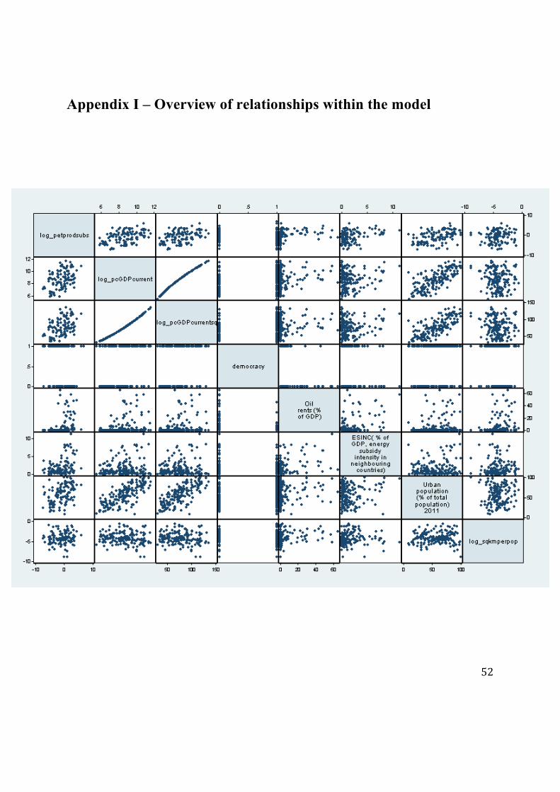
52

Appendix I – Overview of relationships within the model

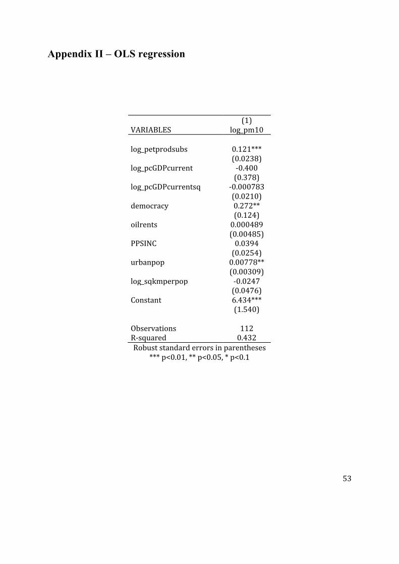
53

Appendix II – OLS regression

(1) VARIABLES log_pm10 log_petprodsubs 0.121*** (0.0238) log_pcGDPcurrent -‐0.400 (0.378) log_pcGDPcurrentsq -‐0.000783 (0.0210) democracy 0.272** (0.124) oilrents 0.000489 (0.00485) PPSINC 0.0394 (0.0254) urbanpop 0.00778** (0.00309) log_sqkmperpop -‐0.0247 (0.0476) Constant 6.434*** (1.540) Observations 112 R-‐squared 0.432 Robust standard errors in parentheses

*** p<0.01, ** p<0.05, * p<0.1

Investigating the relationship between petroleum product ...

Documents

Transcript of Investigating the relationship between petroleum product ...