INVENTORY MODELING Items in inventory in a store Items waiting to be shipped Employees in a firm...

INVENTORY MODELING

• Items in inventory in a store

• Items waiting to be shipped

• Employees in a firm

• Computer information in computer files

• Etc.

COMPONENTS OF AN INVENTORY POLICY

• Q = the amount to order (the order quantity)

• R = when to reorder (the reorder point)

BASIC CONCEPT

• Balance the cost of having goods in inventory to other costs such as:– Order Cost– Purchase Costs– Shortage Costs

HOLDING COSTS

• Costs of keeping goods in inventory– Cost of capital– Rent– Utilities– Insurance– Labor– Taxes– Shrinkage, Spoilage, Obsolescence

Holding Cost RateAnnual Holding Cost Per Unit

• These factors, individually are hard to determine

• Management (typically the CFO) assigns a holding cost rate, H, which is a percentage of the value of the item, C

• Annual Holding Cost Per Unit, Ch

Ch = HC (in $/item in inv./year)

PROCUREMENT COSTS

• When purchasing items, this cost is known as the order cost, CO (in $/order)

• These are costs associated with the ordering process that are independent of the size of the order-- invoice writing or checking, phone calls, etc.– Labor– Communication – Some transportation

PROCUREMENT COSTS

• When these costs are associated with producing items for sale they are called set-up costs (still labeled CO-- in $/setup)

• Costs associated with getting the process ready for production (regardless of the production quantity)– Readying machines

– Calling in, shifting workers

– Paperwork, communications involved

PURCHASE/PRODUCTION COSTS

• These are the per unit purchase costs, C, if we are ordering the items from a supplier

• These are the per unit production costs, C, if we are producing the items for sale

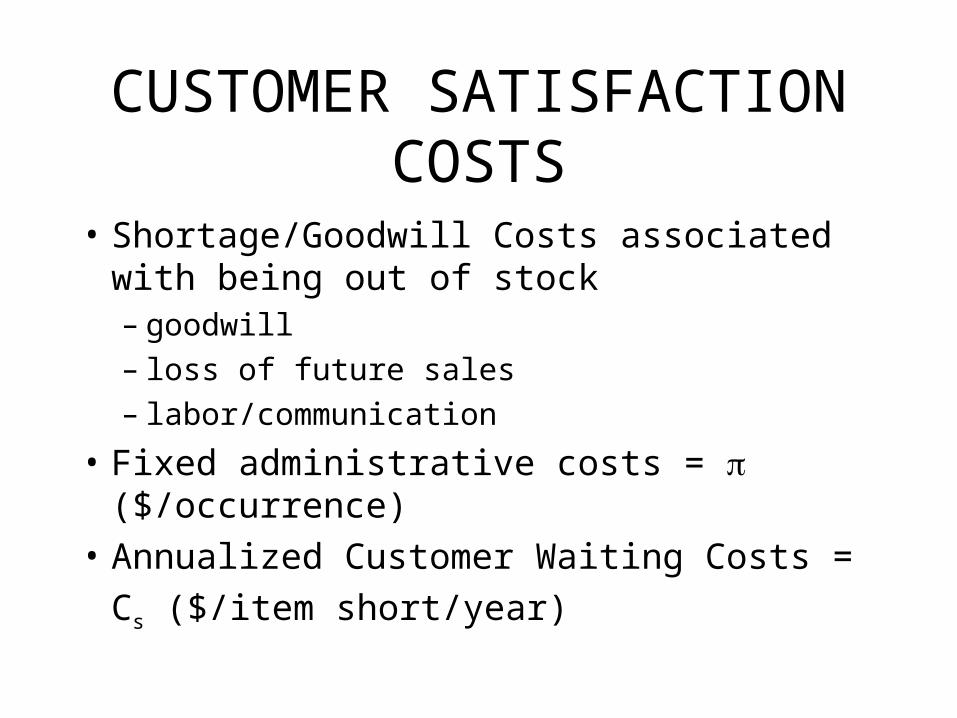
CUSTOMER SATISFACTION COSTS

• Shortage/Goodwill Costs associated with being out of stock– goodwill– loss of future sales– labor/communication

• Fixed administrative costs = ($/occurrence)• Annualized Customer Waiting Costs =

Cs ($/item short/year)

BASIC INVENTORY EQUATION

(Total Annual Inventory Costs) =

(Total Annual Order/Setup-Up Costs) +

(Total Annual Holding Costs) +

(Total Annual Purchase/Production Costs) +

(Total Annual Shortage/Goodwill Costs)

• This is a quantity we wish to minimize!!

REVIEW SYSTEMS

• Continuous Review --– Items are monitored continuously

– When inventory reaches some critical level, R, an order is placed for additional items

• Periodic Review --– Ordering is done periodically (every day, week, 2 weeks,

etc.)

– Inventory is checked just prior to ordering to determine an order quantity

TIME HORIZONS

• Infinite Time Horizon– Assumes the process has and will continue

“forever”

• Single Period Models – Ordering for a one-time occurence

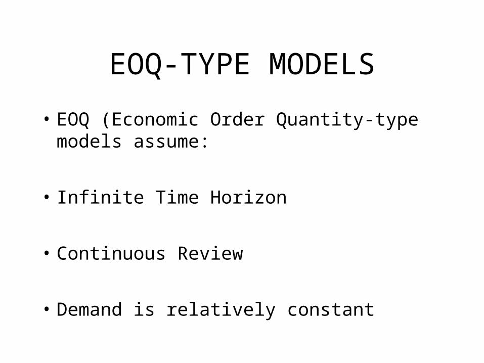
EOQ-TYPE MODELS

• EOQ (Economic Order Quantity-type models assume:

• Infinite Time Horizon

• Continuous Review

• Demand is relatively constant

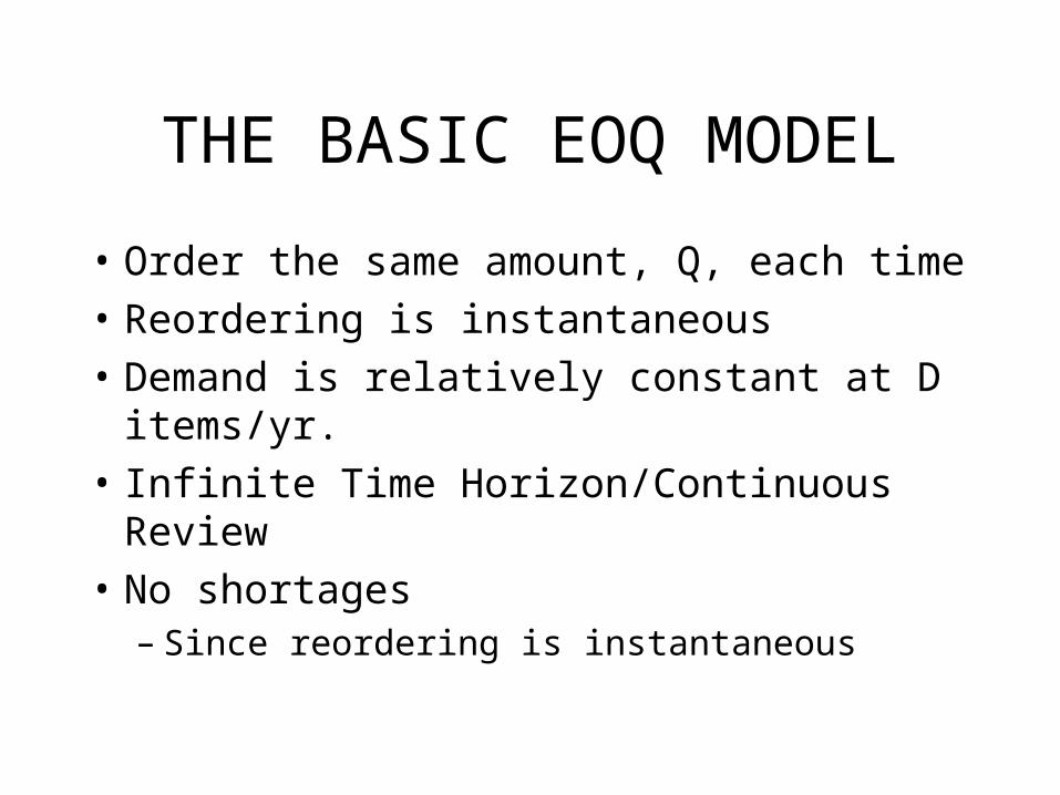
THE BASIC EOQ MODEL

• Order the same amount, Q, each time

• Reordering is instantaneous

• Demand is relatively constant at D items/yr.

• Infinite Time Horizon/Continuous Review

• No shortages – Since reordering is instantaneous

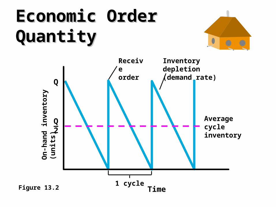
Economic Order QuantityEconomic Order QuantityO

n-h

and

in

ven

tory

(u

nit

s)

Time

Averagecycleinventory

Q

Q—2

1 cycle

Receive order

Inventory depletion (demand rate)

Figure 13.2

THE EOQ COST COMPONENTS

• Total Annual Order Costs:– (Cost/order)(average # orders per year) = CO(D/Q)

• Total Annual Holding Costs:– (Cost Per Item in inv./yr.)(Average inv.) = Ch(Q/2)

• Total Annual Purchase Costs: – (Cost Per Item)(Average # items ordered/yr.) = CD

Economic Order QuantityEconomic Order QuantityA

nn

ual

co

st

(do

llars

)

Lot Size (Q)

Ordering cost

Holding cost

Total cost = Holding Cost + Set-up Cost

Figure 13.3

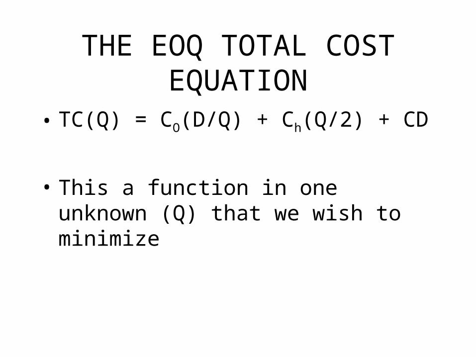
THE EOQ TOTAL COST EQUATION

• TC(Q) = CO(D/Q) + Ch(Q/2) + CD

• This a function in one unknown (Q) that we wish to minimize

SOLVING FOR Q*

• TC(Q) = CO(D/Q) + Ch(Q/2) + CD

Formula EOQ The 2

2

,

002

*

2

2

h

O

h

O

hO

C

DCQ

C

DCQ

Solving

C

Q

DC

dQ

dTC

THE REORDER POINT, r*

• Since reordering is instantaneous, r* = 0

• MODIFICATION -- fixed lead time = L yrs.

r* = LD

But demand was only approximately constant so we may

wish to carry some safety stock (SS) to lessen the

likelihood of running out of stock

• Then, r* = LD + SS

TOTAL ANNUAL COST

• The optimal policy is to order Q* when supply reaches r*

• TC(Q*) = COD/Q* + (Ch/2)(Q*) + CD + ChSS

<==variable cost==> fixed safety

cost stock cost

• The optimal policy minimizes the total variable cost, hence the total annual cost

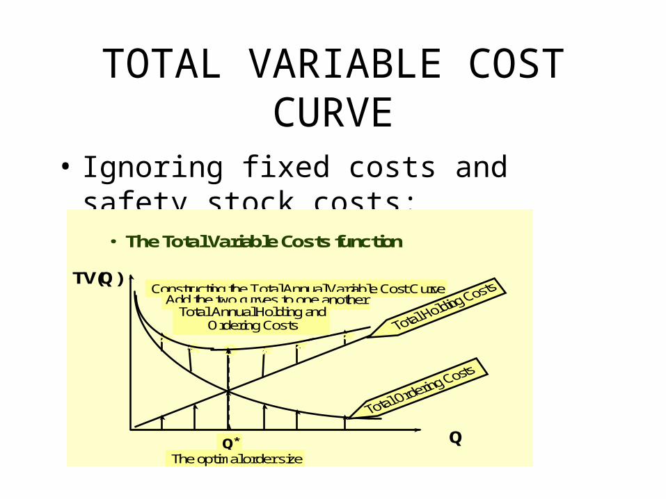
TOTAL VARIABLE COST CURVE

• Ignoring fixed costs and safety stock costs:

• The Total Variable Costs function

Constructing the Total Annual Variable Cost CurveAdd the two curves to one another

* * o * * *Total Annual Holding and Ordering Costs

Q

TV(Q)

Q*

The optimal order size

EXAMPLE -- ALLEN APPLIANCE COMPANY

• Juicer Sales For Past 10 weeks

1. 105 6. 120

2. 115 7. 135

3. 125 8. 115

4. 120 9. 110

5. 125 10. 130

• Using 10-period moving average method,

D = (105 + 115 + …+ 130)/10 = 120/ wk = 6240/yr

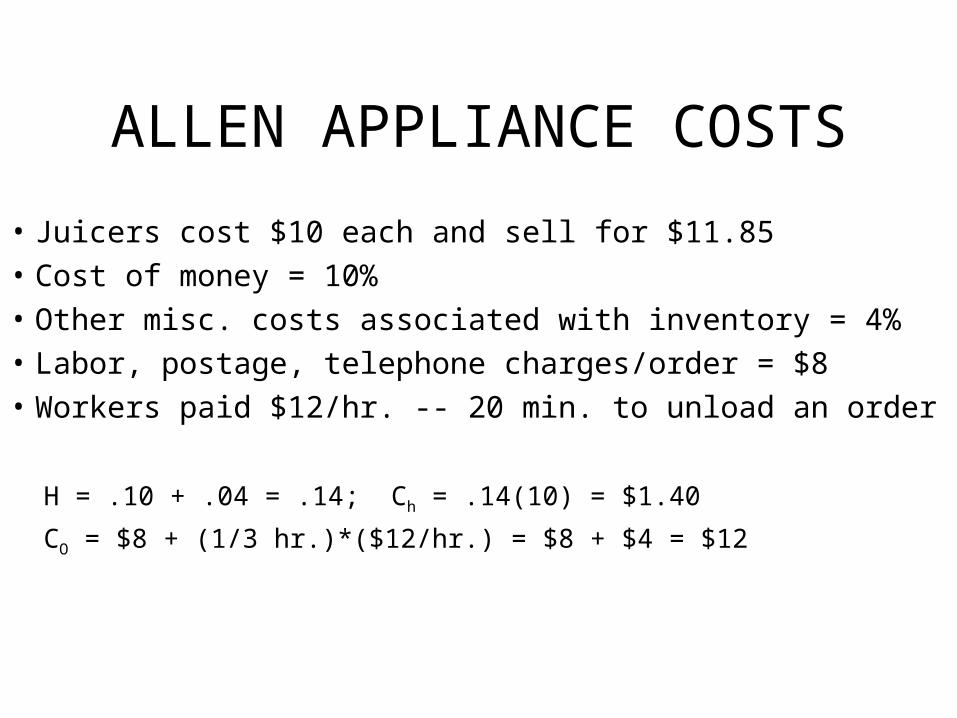
ALLEN APPLIANCE COSTS

• Juicers cost $10 each and sell for $11.85

• Cost of money = 10%

• Other misc. costs associated with inventory = 4%

• Labor, postage, telephone charges/order = $8

• Workers paid $12/hr. -- 20 min. to unload an order

H = .10 + .04 = .14; Ch = .14(10) = $1.40

CO = $8 + (1/3 hr.)*($12/hr.) = $8 + $4 = $12

OPTIMAL ORDER QUANTITY FOR ALLEN

327 *Q toRound

065.32740.1

)6240)(12(22*

h

O

C

DCQ

OPTIMAL QUANTITIES

• Total Order Cost = COD/Q* = (12)(6240)/327 = $228.99

• Total Holding Cost = (Ch/2)Q* = (1.40/2)(327) =$228.90– (Total Order Cost = Total Holding Cost -- except for roundoff)

• # Orders Per Year = D/Q* = 6240/327 = 19.08

• Time between orders (Cycle Time) = Q*/D = 327/6240 = .0524 years = 2.72 weeks

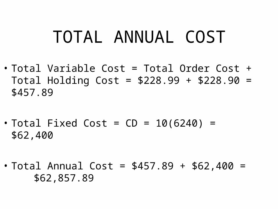
TOTAL ANNUAL COST

• Total Variable Cost = Total Order Cost + Total Holding Cost = $228.99 + $228.90 = $457.89

• Total Fixed Cost = CD = 10(6240) = $62,400

• Total Annual Cost = $457.89 + $62,400 = $62,857.89

WHY IS EOQ MODEL IMPORTANT?

• No real-life model really is an EOQ model

• Many models are variants of EOQ-type models

• Many situations can be approximated by EOQ models

• The EOQ model is relatively insensitive to some pretty major errors in input parameters

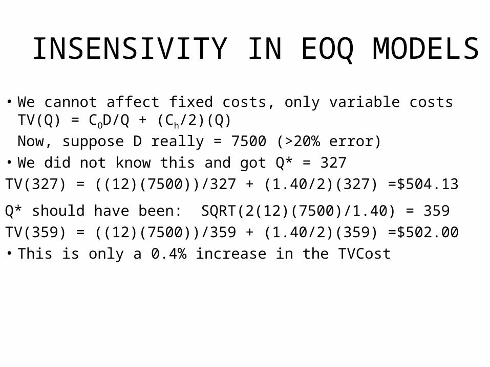
INSENSIVITY IN EOQ MODELS

• We cannot affect fixed costs, only variable costsTV(Q) = COD/Q + (Ch/2)(Q)

Now, suppose D really = 7500 (>20% error)• We did not know this and got Q* = 327

TV(327) = ((12)(7500))/327 + (1.40/2)(327) =$504.13

Q* should have been: SQRT(2(12)(7500)/1.40) = 359

TV(359) = ((12)(7500))/359 + (1.40/2)(359) =$502.00• This is only a 0.4% increase in the TVCost

DETERMINING A REORDER POINT, r* (Without Safety Stock)

• Suppose lead time is 8 working days

• The company operates 260 days per year

• r* = LD where L and D are in the same time units

• L = 8/260 .0308 yrs D = 6240 /year

r* = .0308(6240) 192

OR,

L = 8 days; D/day = 6240/260 = 24

r* = 8(24) = 192

ACTUAL DEMAND DISTRIBUTION

• Suppose we can assume that demand follows a normal distribution– This can be checked by a “goodness of fit” test

• From our data, over the course of a week, W, we can approximate W by (105 + … + 130) = 120

W2 sW

2 = ((1052 +…+1302) - 10(120)2)/9 83.33

DEMAND DISTRIBUTION DURING 8 -DAY LEAD TIME

• Normal

• 8 days = 8/5 = 1.6 weeks, so

L = (1.6)(120) = 192

L2 (1.6)(83.33) = 133.33

L 55.1133.133

SAFETY STOCK

• Suppose we wish a cycle service level of 99%– WE wish NOT to run out of stock in 99% of our

inventory cycles

• Reorder point, r* = L + z.01 L =

192 + 2.33(11.55) 219

• 219 - 192 = 27 units = safety stock = 2.33(11.55)

• Safety stock cost = ChSS = 1.40(27) = $37.80

– This should be added to the TOTAL ANNUAL COST

OTHER EOQ-TYPE MODELS

• Quantity Discount Models

• Production Lot Size Models

• Planned Shortage Model

ALL SEEK TO MINIMIZE THE TOTAL ANNUAL COST EQUATION

QUANTITY DISCOUNTS

• All-units vs. incremental discounts

ALL UNITS DISCOUNTS FOR ALLEN

Quantity Unit Cost

< 300 $10.00

300-600 $ 9.75

600-1000 $ 9.50

1000-5000 $ 9.40

5000 $ 9.00

PIECEWISE APPROACH

• For each piece of the total cost equation, the minimum cost for the piece is at an end point or at its Q*

• If Q* for a piece lies:– above the upper interval limit -- ignore this piece– within this piece -- it is optimal for this piece– below the lower interval limit -- the lower interval

limit is optimal for this piece

• Calculate the total annual cost using the best value for Q for each piece, and choose the lowest

QUANTITY DISCOUNT APPROACH FOR ALLEN

• When C changes, only Ch changes in the formula for Q* since Ch = .14C

Quantity Unit Cost Ch Q* Best Q TC

< 300 $10.00 $1.40 327 ---- ----

300-600 $ 9.75 $1.365 331 331 $61,292

600-1000 $ 9.50 $1.33 336 600 $59,804

1000-5000 $ 9.40 $1.316 337 1000 $59,389

5000 $ 9.00 $1.26 345 5000 $59,325• ORDER 5000

OTHER CONSIDERATIONS

• 5000 is 5000/6240 = .8 years = 9.6 months supply– May not wish to order that amount

• Company policy may be: DO NOT ORDER MORE

THAN A 3-MONTHS SUPPLY = 6240/4 = 1560

• If that is the case, since 1560 is in the interval from 1000 - 5000 and the best Q in that interval is 1000, 1000 should be ordered

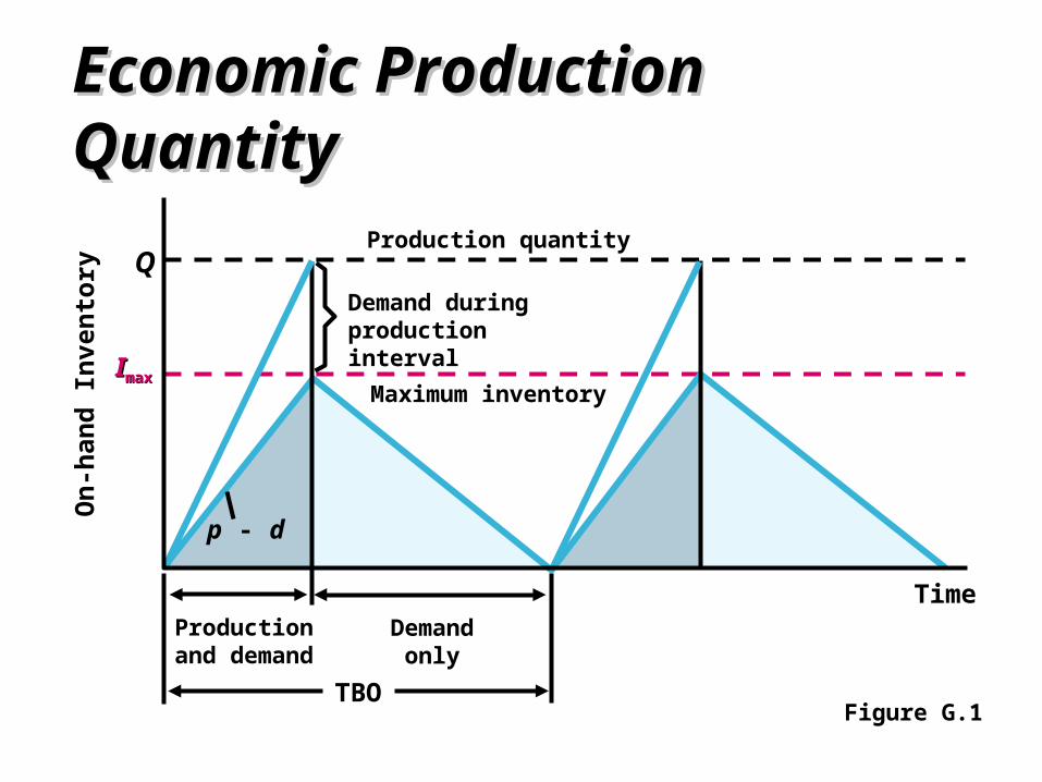
PRODUCTION LOT SIZE PROBLEMS

• We are producing at a rate P/yr. That is greater than the demand rate of D/yr.

• Inventory does not “jump” to Q but builds up to a value IMAX that is reached when production is ceased

• Length of a production time = Q/P

• IMAX = P(Q/P) - D(Q/P) = (1-D/P)Q

• Average inventory = IMAX/2 = ((1-D/P)/2)Q

Economic Production QuaEconomic Production QuantityntityO

n-h

and

In

ven

tory

Time

Figure G.1

Economic Production QuaEconomic Production Quantityntity

Production quantity

On

-han

d I

nve

nto

ry

Q

Time

Figure G.1


Production quantity

On

-han

d I

nve

nto

ry

Q

Time

Figure G.1

Demand during production interval

p - d


Production quantity


On

-han

d I

nve

nto

ry

Q

Time

p - d

Figure G.1


Production quantity


On

-han

d I

nve

nto

ry

Q

Time

p - d

Figure G.1

Production and demand

Demand only

TBO


Production quantity



Demand only

TBO

On

-han

d I

nve

nto

ry

Q

Time

p - d

Figure G.1


Production quantity


Maximum inventory


Demand only

TBO

On

-han

d I

nve

nto

ry

Q

Time

IImaxmax

p - d

Figure G.1

PRODUCTION LOT SIZE -- TOTAL ANNUAL COST

• CO = Set-up cost rather than order cost

• Set-up time for production lead time

• Q = The production lot size

• TC(Q) = CO(D/Q) + Ch((1-D/P)/2)Q + CD

OPTIMAL PRODUCTION LOT SIZE, Q*

• TC(Q) = CO(D/Q) + Ch((1-D/P)/2)Q + CD

SizeLot )/1(

2

)/1(

2

,

002

)/1(

*

2

2

PDC

DCQ

PDC

DCQ

Solving

PDC

Q

DC

dQ

dTC

h

O

h

O

hO

EXAMPLE-- Farah Cosmetics

• Production Capacity 1000 tubes/hr.

• Daily Demand 1680 tubes

• Production cost $0.50/tube (C = 0.50)

• Set-up cost $150 per set-up (CO = 150)

• Holding Cost rate: 40% (Ch = .4(.50) = .20)

• D = 1680(365) = 613,200

• P = 1000(24)(365) = 8,760,000

OPTIMAL PRODUCTION LOT SIZE

449,31)

000,760,8200,613

1(20.

)200,613)(150(2

)/1(

2*

PDC

DCQ

h

O

TOTAL ANNUAL COST

• TOTAL ANNUAL COST =

TV(Q) = CO(D/Q) + Ch((1-D/P)/2)Q =

(150)(613,200/31,449) +

.2(1-613,200/8,760,00)(31,449) = $5,850

TC(Q) = TV(Q) + CD =

5,850 + .50(613,200) = $312,450

OTHER QUANTITES

• Length of a Production run = Q*/P =

31,449/8,760,000 = .00359yrs. = .00359(365)

= 1.31 days• Length of a Production cycle = Q*/D =

31,449/613,200 = .0512866yrs. = .00512866(365)

= 18.72 days• Number of Production runs/yr. = D/Q* = 19.5

• IMAX = (1-613,200/8,760,00)(31,449) = 29,248

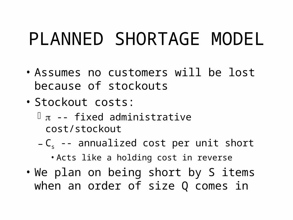
PLANNED SHORTAGE MODEL

• Assumes no customers will be lost because of stockouts

• Stockout costs: -- fixed administrative cost/stockout

– Cs -- annualized cost per unit short • Acts like a holding cost in reverse

• We plan on being short by S items when an order of size Q comes in

PROPORTION OF TIME OUT OF STOCK

• T1 = time of a cycle with inventory

• T2 = time of a cycle out of stock

• T = T1 + T2 = time of a cycle

• IMAX = Q-S

• Proportion of time in stock = T1/T = (Q-S)/Q

• Proportion of time out of stock = T2/T = S/Q

• Avg. inventory = ((Q-S)/Q)((Q-S)/2) = (Q-S)2/2Q

• Average Stockouts = (S/Q)(S/2) = S2/2Q

TOTAL ANNUAL COST EQUATION

• TC(Q,S) = CO(D/Q) + Ch((Q-S)2/2Q) + S(D/Q) + Cs(S2/2Q) + CD

• Take partial derivatives with respect to Q and S and set = 0. We get two equations in the two unknowns Q and S.

*Q

OPTIMAL ORDER QUANTITY, Q*OPTIMAL # BACKORDERS, S*

sh

h

shs

sh

h

O

CC

DQCS

CC

D

C

CC

C

DCQ

**

)(2*

2

EXAMPLESCANLON PLUMBING

• Saunas cost $2400 each (C = 2400)

• Order cost = $1250 (CO = 1250)

• Holding Cost = $525/unit /yr. (Ch = 525)

• Backorder Good will Cost $20/wk (CS = 1040)

• Backorder Admin. Cost = 10/order ( = 10)

• Demand = 15/wk (D=780)

RESULTS

backorders20 are e when ther74order Re

201040525

)10)(780()74)(525(*

74)1040)(525(

)10*780(

1040

1040525

525

)780)(1250(2*

2

S

Q

What IF Lead Time Were 4 Weeks?

• Demand over 4 weeks = 4(15) = 60

• Want order to arrive when there are 20 backorders.

• Thus order should be placed when there are 60 - 20 = 40 saunas left in inventory

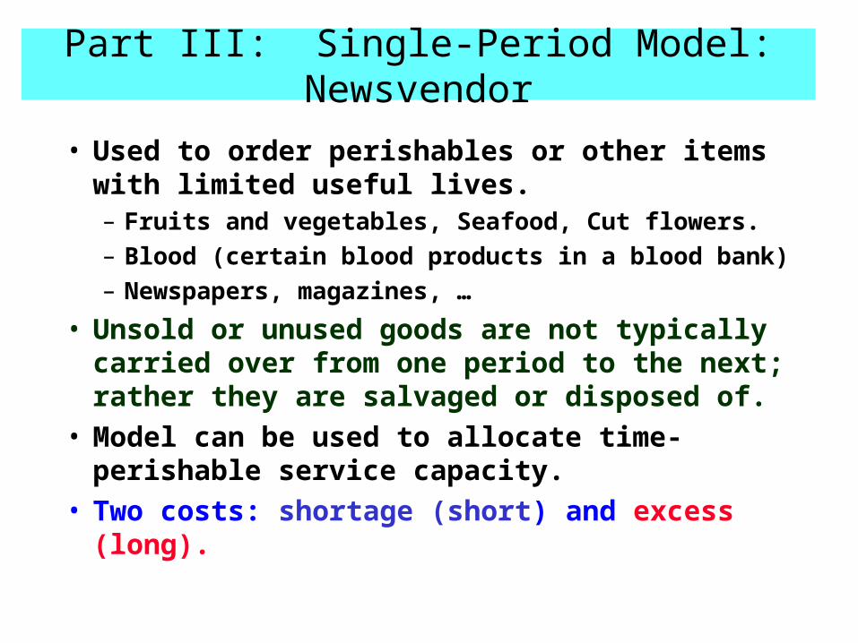
Part III: Single-Period Model: Newsvendor

• Used to order perishables or other items with limited useful lives.– Fruits and vegetables, Seafood, Cut flowers.

– Blood (certain blood products in a blood bank)

– Newspapers, magazines, …

• Unsold or unused goods are not typically carried over from one period to the next; rather they are salvaged or disposed of.

• Model can be used to allocate time-perishable service capacity.

• Two costs: shortage (short) and excess (long).

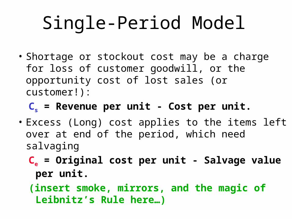
Single-Period Model

• Shortage or stockout cost may be a charge for loss of customer goodwill, or the opportunity cost of lost sales (or customer!):

Cs = Revenue per unit - Cost per unit.

• Excess (Long) cost applies to the items left over at end of the period, which need salvaging

Ce = Original cost per unit - Salvage value per unit.

(insert smoke, mirrors, and the magic of Leibnitz’s Rule here…)

The Single-Period Model: Newsvendor• How do I know what service level is the best one, based

upon my costs?• Answer: Assuming my goal is to maximize profit (at

least for the purposes of this analysis!) I should satisfy SL fraction of demand during the next period (DDLT)

• If Cs is shortage cost/unit, and Ce is excess cost/unit, then

SLC

C Cs

s e

Single-Period Model for Normally Distributed Demand

• Computing the optimal stocking level differs slightly depending on whether demand is continuous (e.g. normal) or discrete. We begin with continuous case.

• Suppose demand for apple cider at a downtown street stand varies continuously according to a normal distribution with a mean of 200 liters per week and a standard deviation of 100 liters per week:

– Revenue per unit = $ 1 per liter

– Cost per unit = $ 0.40 per liter

– Salvage value = $ 0.20 per liter.

Single-Period Model for Normally Distributed Demand

• Cs = 60 cents per liter

• Ce = 20 cents per liter.

• SL = Cs/(Cs + Ce) = 60/(60 + 20) = 0.75

• To maximize profit, we should stock enough product to satisfy 75% of the demand (on average!), while we intentionally plan NOT to serve 25% of the demand.

• The folks in marketing could get worried! If this is a business where stockouts lose long-term customers, then we must increase Cs to reflect the actual cost of lost customer due to stockout.

Single-Period Model for Continuous Demand

• demand is Normal(200 liters per week, variance = 10,000 liters2/wk) … so = 100 liters per week

• Continuous example continued:– 75% of the area under the normal curve

must be to the left of the stocking level.– Appendix shows a z of 0.67 corresponds to a

“left area” of 0.749 – Optimal stocking level = mean + z () = 200

+ (0.67)(100) = 267. liters.

Single-Period & Discrete Demand: Lively Lobsters

• Lively Lobsters (L.L.) receives a supply of fresh, live lobsters from Maine every day. Lively earns a profit of $7.50 for every lobster sold, but a day-old lobster is worth only $8.50. Each lobster costs L.L. $14.50.

• (a) what is the unit cost of a L.L. stockout?

Cs = 7.50 = lost profit

• (b) unit cost of having a left-over lobster?

Ce = 14.50 - 8.50 = cost – salvage value = 6.

• (c) What should the L.L. service level be?

SL = Cs/(Cs + Ce) = 7.5 / (7.5 + 6) = .56 (larger Cs leads to SL > .50)

• Demand follows a discrete (relative frequency) distribution as given on next page.

Lively Lobsters: SL = Cs/(Cs + Ce) =.56

Demand follows a discrete (relative frequency) distribution:

Result: order 25 Lobsters, because that is the smallest amount that will serve at least 56% of the demand on a given night.

Probability that demand

Demand

Relative Frequency

(pmf)

Cumulative Relative

Frequency (cdf)

will be less than or equal to x

19 0.05 0.05 P(D < 19 )

20 0.05 0.10 P(D < 20 )

21 0.08 0.18 P(D < 21 )

22 0.08 0.26 P(D < 22 )

23 0.13 0.39 P(D < 23 )

24 0.14 0.53 P(D < 24 )

25 0.10 0.63 P(D < 25 )

26 0.12 0.75 P(D < 26 )

27 0.10 you do P(D < 27 )

28 0.10 you do P(D < 28 )

29 0.05 1.00 P(D < 29 )

* pmf = prob. mass function

INVENTORY MODELING Items in inventory in a store Items waiting to be shipped Employees in a firm...

Documents

Transcript of INVENTORY MODELING Items in inventory in a store Items waiting to be shipped Employees in a firm...