INTRODUCTORY LECTURES ON RESEARCH METHODOLOGY

Adigun Agbaje, Department of Political Science, University of Ibadan, Nigeria.

And

A. Isma’il Alarape

Department of Psychology, University of Ibadan, Nigeria.

SEPTEMBER 2002, 2003, 2004, 2005, 2006, 2009, 2010

2

PREFACE TO 2006 EDITION This edition features a new section on computer application contributed by Dr. A.I. Alarape of the Department of Psychology, University of Ibadan. The new section introduces participants to the application of the Statistical Package for the Social Sciences (SPSS) and OpenCode in data analysis, thus complementing the manual method to which participants were exposed in the past. The goal is to ensure that each participants acquires functional level of computer literacy in this regard on which (s)he can build thereafter. Adigun Agbaje and A. Isma’il Alarape Ibadan. 10 September 2006

3

PREFACE

In 2001, I was invited by the National War College, Abuja, to deliver a series of introductory lectures on research methodology. It was not clear to me then that I was expected to prepare written texts ahead of the lectures. Subsequently, I agreed to prepare such texts after the lecture but in good time for the use of Course 10 (2001/2002) participants. Alas! I could not deliver on this promise in the life of Course 10, and it took the persistence of (then) Commodore O. Abegunde and “friendly fire” from (then) Brigadier General O. Azazi for the written texts to be completed. A principal objective of the work of the college is “to prepare … participants for higher-level policy, command and staff functions”, requiring “inquisitiveness, an analytical mind, logical reasoning and sound decision making ability”. In this context the College has, in its own words, “continued to place a great deal of emphasis on research”. These introductory lectures have taken this into consideration, along with the College’s observation that most participants in its course of study and research have no previous formal exposure to research methodology. The lectures, therefore, in a step-by-step manner, address issues in the research process from a “nuts and bolts” perspective. They adopt a practical, “how-to-do-it” approach while at the same time highlighting aspects of the theoretical and technical bases of the research process. The lectures seek to equip participants with the basic tools of scientific research applicable not only in their current spheres of activity but also in the wider arena of human society at large. As introductory lectures, they do not pretend to be exhaustive or definitive. Rather, they seek to emphasize brevity and clarity in their invitation to participants to get familiar with research methodology – and then take the additional step of consulting with one another, the College’s teaching and research staff, as well as relevant texts, including but not restricted to the two recommended in the pages ahead. Adigun Agbaje Ibadan 02 September, 2002.

4

I. NATURE AND LANGUAGE OF SCIENTIFIC RESEARCH This first set of lectures introduces participants to the essence of scientific research in the social sciences and the humanities. In summary form, the lecture highlights the nature of scientific research and why it is to be preferred to non-scientific methods of acquiring, validating and updating knowledge and belief. It also highlights, with specific reference to defence and security studies, types and sources of data for scientific research, the range of issues and events that could be researched into in this broad area, as well as problems that could be encountered in conducting scientific research into defence/security matters. Participants are also introduced to key elements in the language of scientific research. The lectures end with guidelines on the writing of research proposals. At the end of this first series of lectures, it is expected that participants will be able to: know and identify the various methods of acquiring, validating and anchoring

knowledge/belief; identify types and sources of data for scientific research in general and in defence and

security issues in particular; list topics on which scientific research can be conducted in the broad area of defence and

security; appreciate problems in conducting scientific research in general and in defence and

security studies in particular; understand basic elements of the language of scientific research, and fully appreciate the nature of scientific investigation.

1. NATURE AND IMPORTANCE OF SCIENTIFIC RESEARCH On a daily basis, we acquire new knowledge, validate or reject long-held ones, reaffirm old beliefs, and get on with our lives. How do we do all this, given the mass of information (data) that we do have to process from day to day? Although the process of validating or acquiring or rejecting knowledge and our beliefs might appear to be random, there is an order, a systematic dimension, to it. Imagine that you are confronted with these two statements: STATEMENT ONE: “Trained, professional infantry soldiers do better in battle than

untrained, inexperienced conscripts”. STATEMENT TWO: “Trained, experienced politicians do a better job of running

democratic governance than ordinary citizens”. How do you react to such statements? Would the response to both statements not be affirmative, confirming the accuracy of the two observations? Does it not agree with reason, common sense, all that we know, our intuition, that soldiers, trained to kill and experienced in battle, would do better on the battle field than a rabble of conscripts that are untrained, inexperienced and probably pressed to war against their wish? Does it not agree with reason, common sense, history, and intuition that politicians have more skills in running government than ordinary citizens, and would therefore do a better job in this regard?

5

Right. And Wrong. What the scientific method of acquiring/validating knowledge and belief shows clearly is that what appears right to common sense, reason, intuition and experience can in fact be wrong. Take this report that touches on the first statement, for instance: A United States army colonel, Colonel S.L. Marshall, conducted a scientific study of men in about 400 infantry companies during the Second World War. The study’s objective was to investigate the men’s reactions to battle. His finding: On average, only 15 percent of troops fired their guns at all in battle, even when their positions were directly under attack and their lives in danger. The study showed that the men tended to fire their weapons when others, especially officers, were present, but not when more isolated. The research noted that the men’s “unwillingness to fire had nothing to do with fear, but reflected a disinclination to kill when there was ‘no need’” (Giddens, 1993: 357). Think also about the following, which touches on STATEMENT TWO: It is often forgotten that the original, classical, definition and practice of democracy involved direct and physical involvement in governance by all citizens. The modern day practice of democracy, involving indirect participation of the people in government through their elected representatives (who have over time become a more or less “professional” group called politicians) is, in fact a relatively new development in human history. It is also at variance with the original meaning of democracy. It does appear, therefore, that sense can disappear from “common sense”, our beliefs can fail us or in fact reflect the level of our ignorance, while “received wisdom” can reflect anything but wisdom, in our search for knowledge and its validation. 2. METHODS OF ACQUIRING/VALIDATING KNOWLEDGE The two examples highlighted above illustrate the point that, in knowledge acquisition, all that glitters is not gold. Many roads lead to the market, we are reminded. The literature identifies four principal ways by which we acquire/validate knowledge and belief: three are non-scientific while one is scientific. The non-scientific methods are those of tenacity, authority and intuition. (a) Non-Scientific Methods

(i) The Method of Tenacity: By this method, we know/believe because we know/believe. In other words, our knowledge/belief derives from and is validated by what we hold on to as our knowledge/belief. We know/believe that soldiers would do a better job of prosecuting war because that is what we know/believe. We believe in God because we believe in God.

(ii) The Method of Authority: By this method, knowledge/belief is anchored on

authority. We know/believe because authority (somebody or something with the right, power or special knowledge to say so) says so. We know that soldiers do better in battle because General T.Y. Danjuma says so. We believe in God because the Holy Quran and the Holy Bible say so. This authority can take either of several forms or a combination thereof. These include: * Expertise * Tradition/History

6

* Public Sanction * Religion/Superstition/Mystic

(iii) The Method of Intuition: As the name implies, knowledge is acquired/validated here with reference to reason or intuition, otherwise called common sense. Thus, it agrees with common sense to know that God exists, or that Man is created free, or that soldiers have comparative advantage on “killing fields”.

These are the three methods of acquiring/validating knowledge that are identified as non-scientific. In fact, they are equally pre-scientific in the sense that the method of science grew out of a felt need to addresses perceived weaknesses in these non-scientific methods. Such weaknesses include the following:

It is difficult, if not impossible to resolve conflicts among contending perspectives/positions under any of these non-scientific methods. Thus, for instance, if A believes in God because A believes in God, and B does not believe in God because B does not, how do we get this resolved, or assess which position is better/superior?

Arising from this problem is the fact that the non-scientific ways of acquiring/validating knowledge do not facilitate progress.

Knowledge derived from any of these methods tends to be space-specific, source-specific, time-bound, not universal, and highly perishable.

In describing the transition from the non-scientific methods to the scientific method of knowledge acquisition, a philosopher of science in the early 20th century, Charles Peirce, has this to say: To satisfy our doubts …, it is necessary that a method be found by

which our beliefs may be determined by nothing human, but by some external permanency – by something upon which our thinking has no effect. The method must be such that the ultimate conclusion of every man shall be the same. Such is the method of science. Its fundamental hypothesis is this - there are real things, whose characters are entirely independent of our opinions about them.

(b) The Scientific Method By this method, we acquire knowledge through empirical investigation conducted according to laid down and well-defined rules and procedures for collecting, analyzing and evaluating information (also called data). The scientific method involves the application of the rules of science in the search for knowledge. Thus, we get to know because widely accepted scientific procedures lead us to know. As Auguste Comte, a philosopher, stated long ago: “observation of facts is the only solid basis of human knowledge”. Such observation, recording and evaluation of facts are what constitute scientific research, utilizing the scientific method of acquiring/validating knowledge. Characteristics of the method include the following:

7

It produces/validates knowledge with reference to standards and procedures that are largely external to the individual, are more or less permanent, and are not affected by human thinking.

It is a critical method. It emphasizes openness in the search for knowledge, insisting that all arguments and procedures be reported as fully and publicly as possible.

It is a systematic and controlled method. A scientific investigation must follow a well-ordered, tightly disciplined procedure.

It is empirical, grounded in observation and experience. It leads to the collection of evidence and the testing of such evidence. In other words, the method largely focuses on what is, rather than what ought to be, in terms of the evidence from which it seeks to validate knowledge or belief.

The scientific method allows for replication. Because it insists on full disclosure

and explicitness of procedures, the method makes it possible for a particular study to be repeated by others across time and space with a view to corroborating or refuting its findings. It thus leads to knowledge that can be transmitted across time and space, since it is itself a social process.

The scientific method is self-correcting. It is provisional. There is no “final

solution” under this method. It is open-ended. It has no room for oracles or infallibility. In fact, the logical essence of the method emphasizes that attempts be made to test the falsifiability of established “facts”, rather than proving such “facts” to be true.

Finally, the ultimate goal of the method is to seek explanation, rather than mere

description. It seeks to answer the “why” question. The Scientific Process As indicated above, the scientific method prescribes laid down steps and procedures for knowledge acquisition that are more or less universally accepted. This is the essence of the research process, presented below in the form of the research cycle as well as in terms of the basic steps and stages in scientific investigation. As a cycle, the research process takes off in terms of the identification of a research problem or idea. No meaningful scientific research can be undertaken without a valid statement of the problem the research seeks to address. A research problem is not the same as problems in everyday life. Rather, it is a problem that arises from the state of received wisdom/knowledge or existing practice with regard to the topic under investigation. It shows clearly the gap to be filled, issues to be clarified, by the proposed study. Problem Problem Conclusion Theory Solution Obstacles Test Previous Experience

8

After the problem has been articulated, the next stage is to consult existing literature on the state of knowledge or experience in the field. This then leads to the actual conduct of the study under consideration. The study generates its own conclusion(s) that, of course, should relate to and address the original research problem that led to the study in the first instance. In more elaborate form, basic steps in research utilizing the scientific method include the following: Step I: Formulate the Research Idea/Problem. This can emanate from:

- the researcher’s interest/experience/observation; - the researcher’s ongoing work; - matters arising from the work of others.

Step II: Conduct a Literature Review: Go through libraries and other resource centers

(including electronic ones) and review work already done in the area under investigation.

Step III: Identify and define your key concepts. Step IV: Formulate Research Questions, Objectives and Hypotheses as appropriate. Step V: Collect your Data. Step VI: Analyse and Discuss your Data. Step VII: Draw Appropriate Conclusion(s). Step VIII: Write the Research Report. In more detail, this translates as basic stages in research as indicated below: Steps in Conducting Scientific Research Problem Stage 1. Identify the PROBLEM area. 2. Survey the LITERATURE relating to the problem; in light of the literature, explain the

problem for investigation in clear, specific terms. 3. Identify and define relevant CONCEPTS or VARIABLES and relate them to each other

in testable HYPOTHESES, answerable research questions and research objectives as appropriate.

Planning Stage 4. Construct the RESEARCH DESIGN to maximize internal and external validity:

(a) select your subjects if required; (b) control and/or manipulate variables if required; (c) establish criteria to evaluate outcomes;

9

(d) engage in instrumentation – select or develop measuring instrument(s), if necessary.

5. Specify the DATA COLLECTION procedures, and 6. Select and specify the DATA ANALYSIS methods. Execution Stage 7. Execute research as planned; 8. ANALYSE the data, answering research questions, meeting research objectives and

testing hypotheses specified; report findings of tests and any additional information of interest to the research problem.

9. EVALUATE the results and draw CONCLUSIONS relating these to the problem area. How Scientific Knowledge is Produced Basically, there are two ways by which scientific knowledge can be produced. These are through the methods of induction and deduction. Induction is a process of moving from specific observations to a general conclusion. The researcher in this regard takes the following steps: First he or she observes phenomena and records them. He/she studies data so recorded for possible patterns and regularities. Finally, he/she seeks explanation(s) to such patterns where they exist. It is at this final

stage that what is called a theory (more on this later), in the form of a general principle that explains what has been discovered, can emerge.

In the second method of deduction, there is movement from a theory to specific observations. In other words, theory precedes observation. It involves the following steps:

On the basis of a theory, an investigator predicts certain phenomena. Next, the investigator observes and collects data to ascertain whether the

phenomena occur as predicted. Typically, however, scientific research involves both deduction and induction. A researcher may start with a theory and deduce certain phenomena that he then sets out to observe. If successive observations do not fit the theory, then the theory can be revised and, ultimately, rejected. Observations then lead to a new theory through induction. Scientific research can be either quantitative or qualitative in method and approach. A quantitative approach relies heavily on quantitative (statistical) data in the form of numbers collected through empirical observation or from statistical digests. Qualitative approaches rely more on data that are in the form of words rather than numbers. While quantitative data are analysed through the use of descriptive and inferential statistical tools with a view to testing hypotheses and offering explanations, qualitative data are categorized into themes and evaluated with a view to describing or discovering phenomena. From the non-scientific to the scientific: Any meeting point? So far, I have emphasized the differences between non-scientific and scientific methods of acquiring knowledge. For the avoidance of doubt, however, it must be noted that these methods

10

are often complementary. In practical terms, a scientific investigator often makes the initial decision on what to study on the basis of his belief, some authority, or intuition. He can thereafter proceed to conduct the study in a scientific manner. Is science about substance, or about method? The second point that I want to make in concluding this section relates to the meaning of science. Science is about method, not about substance. For this reason, any discipline or investigation that applies the method of science to its enterprise is fit to be described as scientific. As others have noted, “the subject-matter being studied does not determine whether or not the process is called scientific. It makes no difference whether the investigation is in the fields traditionally held to be sciences, such as Chemistry or Physics, or is in the various areas of human relations, including … social sciences. The activity of an investigator is scientific if he correctly uses the scientific method, and the investigator is a scientist if he uses the scientific method in his thinking and searching for information”. 3. LANGUAGE OF SCIENTIFIC RESEARCH The science or study of methods of research, otherwise called research methodology, has its own language and key words. It is appropriate at this stage to briefly highlight the meaning of words that we will continue to encounter as we study and apply the scientific method. These include population (or universe), sample, subject, parameter, statistic, concept, variable, hypothesis and theory. Population (or universe) refers to the entire group of people, events, institutions, issues, countries that is the target or subject of investigation. All military coups in Africa constitute the population for a study of military coups on the continent. Sample refers to any sub-set or sub-group of the population. Thus military coups in the 1960s (or in Sierra Leone or Eastern Africa), in so far as these are sub-sets, constitute a sample of military coups in Africa. The critical point here is the target population, which varies from study to study. A subject is a single member of a sample. Thus, the January 1966 coup in Nigeria is a subject in the sample of African coups that occurred in the 1960s drawn from the population of all military coups in Africa. A parameter is an attribute of a population. An example would be the success rate of all coups in Africa. A statistic is an attribute of a sample. An example is the success rate of a sample of military coups in Africa. A Concept is an abstraction based on characteristics of perceived reality. It is a word or general notion that expresses generalizations from particulars. For instance, “weight” is a concept that

11

expresses numerous observations of the extent to which things are more or less heavy, just as security expresses observations about the extent of safety and freedom from danger or anxiety. From the preceding paragraph, it is clear that one way of defining a concept is through the use of other concepts. Thus, I define weight above by referring to heaviness. I also see security in relation to safety, danger and anxiety. This is what is called conceptual definition – defining a concept (word) with the help of other concepts (words). Another way of defining concepts, especially in certain types of research involving quantitative data, is through what is called operational definition. This definition specifies the process by which a concept is to be measured. Operational definition of weight will specify specific measurement procedure (in pounds, kilogrammes, etc). Security can be operationally defined as zero strikes, zero conflicts, etc within a specified period. A variable is a concept (symbol or characteristic) whose values can vary. In other words, it is a concept that can take more than one value, a quality or characteristic that varies among the subjects of investigation. There are different types of variables. A continuous variable is one that is capable of taking on an ordered and theoretically infinite set of values. Examples are the variables of age, income, casualty, height and weight. A categorical (or discrete) variable on the other hand is one capable of taking on only a specific set of values of a discontinuous nature, with each value being individually distinct from the others. Examples are: sex, religion and marital status. An independent variable is the presumed cause/influence/explanation of the dependent variable, whose values are presumed to be dependent on or affected by the independent variable. In other words, the dependent variable is the presumed effect or function of the independent variable. Other types of variables are competently explained in relevant texts. An hypothesis is a conjectural statement linking two or more variables (at least one independent and one dependent) in a hypothesized relationship. Much of scientific research involves the collection and analysis of data to uphold or falsify such hypotheses. Concepts and variables constitute the building blocks of scientific research. While certain types of research (especially those involving non-quantitative data) can be conducted without hypotheses, which essentially link concepts and variables together, no research of a scientific nature can be conducted in the absence of concepts and variables. Finally, as indicated earlier, the ultimate goal of scientific research is to discover powerful theories that provide explanation for observed phenomena. Simply put, a theory is a set of interrelated concepts, definitions and propositions that present a systematic view of phenomena by specifying relations among variables with the purpose of explaining, predicting and controlling the phenomena. The natural and physical sciences have been more successful in theory-building than the social sciences and the humanities for obvious reasons. One reason is that human beings are definitely more complex and more unpredictable than such inanimate objects as rocks. Discovering theories that help to explain, predict and control such erratic entities becomes a very difficult task indeed.

12

A second major reason has to do with measurement problems, which are more acute in the social sciences than in the physical sciences. How do we, for instance accurately measure such things as unemployment, instability, extent of freedom, corruption and impact of public policy? 4. PROBLEMS AND PROSPECTS OF CONDUCTING RESEARCH ON DEFENCE

AND SECURITY IN AFRICA This leads us to obstacles to scientific research in general as well as in the specific instance of researching into defence and security matters in African contexts. Against this background, it is also important to itemise openings and opportunities for such research. This section of the lecture itemizes the problems and areas that can be researched into. The next section identifies appropriate data types and sources for defence and security studies. The problems and obstacles that are often listed include the following (in no specific order): Adequacy/Accuracy of Data Resource Constraints Poor library/archival facilities Low level of culture of research Institutional censorship Official Secrets and Access Institutional rivalry Bureaucracy Recency of Events/Issues Poor IT Base and general infrastructure inadequacies.

In the area of deciding on what to study, the Defence College has developed a commendable and helpful approach. It makes available to participants a comprehensive list of research topics from which to select. Participants should avail themselves of this opportunity under the guidance of their supervisors early in the Course. Where such a facility is unavailable, researchers are advised to do a comprehensive survey of both published and unpublished materials before zeroing in on topic options. In the context of a supervised research project, the ultimate decision on what to study is usually made by the supervisor to ensure that conformity with the tradition and needs of the institution. In addition to possibilities highlighted above, the following broad areas can also offer suggestions on what to study. These are:

Military technology: History, modern weapons and weapons system; Philosophy, theory and ethics of war and peace; Laws of War; Military Law; Defence Economics; Conduct of War; Tactics (Land, Naval and Air) Logistics; Intelligence;

13

Guerrilla Warfare and Counter-guerrilla Warfare; Communications/ Propaganda; Defence Management; and Broad Social, Economic and Governance Issues

To summarise: the decision on what to study in a supervised context as is the case with the Defence College is ultimately not one to be made by the researcher. The decision lies with the College, appropriate committees, and the person designated as Supervisor of the research work. None the less, as much as possible, one or a combination of the following helps to facilitate topic selection:

Look not only at the usual places but also at unusual places! Go through what others have done

- At the College - Elsewhere, including outside Nigeria

Utilise Comparative Advantage, including - Your own experience - Experience of others to whom you have access

Ponder over contemporary events and issues The dos and don’ts of topic selection (whether in a supervised or unsupervised research environment) include the following:

Select a topic that you are interested in. Avoid a topic that is too ambitious. Avoid topics that are likely to make you too emotional or over which you have an

axe to grind with someone, a group, institution, or any other entity. Select a topic in which you are likely to make original contribution to knowledge.

5. TYPES AND SOURCES OF DATA FOR SCIENTIFIC RESEARCH Once a decision is taken on the research topic, the next step is to identify the type(s) of data required for the survey and their source(s). In the past, it was probably much easier for a student of defence and security to decide on what to study and where to go for data. Then, defence and security were defined mainly in the military terms of the acquisition, husbanding, expansion and retention of the monopoly of the means of violence. Over the years, defence and security have come to be defined also in non-military, non-forcible manners. They now embrace all aspects of society – from economy to culture, infrastructure, agriculture, education, health, the environment, group rights and IT, among others. Again, therefore, the exhortation is to look for both the usual types and sources of data and the unusual. These include:

Historical/Archival data (available mainly in libraries and private collections). Experimental data (generated through the setting up of artificial laboratory – type

situations).

14

Field data (essentially survey data with individual as unit or case). Aggregate data (individual not unit but group e.g. census, data on military

hardware, UN publications; publications of Institutes and Centres for the Study of War, Peace, Economics, Agriculture, etc.

Public Records (Obtainable from records that are publicly available. Broad and can overlap with others. Examples: data on government expenditure, crime statistics, roll-call-vote-voting records of legislators).

6. WRITING A RESEARCH PROPOSAL It is often required that the researcher work out a research proposal before setting out on the study, detailing what he seeks to study, why, how the study is to be conducted and reported, as well as the significance of the study. The minimum ingredients of such a proposal comprise the following:

Statement of the Problem: Questions to answer here include: Is it clear and researchable? Is it a real research problem, or a “straw man” created to legitimize an unnecessary study? Will it extend the frontiers of knowledge, or improve policy and practice? Is the problem located within the context of previous studies or experience/practice?

Study Objectives, Research questions and Hypotheses: One of these could be

adequate, although nothing stops a researcher from listing the three. Essentially a statement of objective can also be turned into a research question and an hypothesis.

Proposed Methods: Should include, as appropriate, sampling methods, data

collection methods, and data analysis methods.

Scope (in time and space as appropriate) and Limitations of/to the study

Literature Review (often depends on institutional and other factors). In doing this, provide a hierarchy from very relevant literature to relevant and then background literature.

Significance of Study

Plan of Study: A summary of how the study will be reported in terms of chapters,

etc. REFERENCES Giddens, A. (1993). “War and the Military” in his Sociology, Cambridge: Polity Press. FURTHER READING Johnson, J.B. and Joslyn, R.A. (1991). Political Science Research Methods, Washington, D.C.:

Congressional Quarterly Inc; Chapters 1 – 3. Rudestam, K.E. and Newton, R.R. (1992). Surviving Your Dissertation: A Comprehensive

Guide to Content and Process, Newbury Park, CA: Sage Publications, Chapters 1 and 2.

15

II. RESEARCH DESIGN: PLANNING YOUR RESEARCH

The decision on what to study has to be followed quickly by a period of planning for the study, or designing the research to enhance its validity. These series of lectures introduce participants to the planning stage of the research process– its meaning, purpose, and constituents (such as issues relating to sampling and measurement). At the end of the lectures, participants are expected to:

(a) know the meaning and essence of research designs and (b) know and be capable of utilizing sampling and measurement scientifically and

validly in their research work 1. MEANING OF RESEARCH DESIGN A research design is the total plan of a given study. It outlines how the study will be executed with the minimum of complications. In other words, research design is to scientific research what a building plan is to building construction. You can build without a plan, but it would be less hazardous and more acceptable to the wider community to have a plan before you begin to erect your building. Essentially, a research design maps out the plan, structure and strategy of scientific investigation. This helps to ensure that research questions are answered easily and accurately, that research objectives are met in an acceptable manner, and that hypotheses are validly and accurately tested. In mapping the structure and strategy of the study, the design outlines key variables as well as methods to be used to gather and analyse data with a view to tackling problems to be encountered during the research in a manner that does not jeopardize the overall objective(s) of the research. Thus, it is not only akin to a building plan; it also literally provides a road map for the researcher keen to answer his/her research questions as validly, accurately, objectively and economically as possible. In other words, the design outlines:

observations that will be made to answer questions posed by the research as accurately, validly, objectively and economically as possible,

how the observations will be made, analytical and statistical procedures (if required) to be applied on data so collected,

and if the goal of research is to test hypotheses, how the test is to be executed.

Developing a good research design is as important as developing good research questions, objectives and hypotheses. Factors that determine the choice of research design include the following: (a) Purpose of Investigation – Is it:

(i) Exploratory? If so, you do not require a sophisticated or complicated design. In a sense, an exploratory study is easiest to conduct, since not much is expected of it. It is the kind of study that covers uncharted territory, a

16

pioneering study of sorts, and the research community tends not to be too critical of its methods or expected too much of its findings.

(ii) Descriptive? If so, you equally do not require a very sophisticated or

complicated design – although more is expected of your study. This is assumedly a higher – level enterprise compared to exploratory studies.

(iii) Explanatory? This is the highest and most demanding level of investigation.

It requires a sophisticated design.

(b) Practical Limitations (i) Ethical Considerations (ii) Data Difficulties (access, lack etc) (iii) Resource Constraints (time, money, expertise)

2. PURPOSE OF PLANNING: ENHANCING VALIDITY Good planning helps to maximize the validity of the study under question. In this regard, however, there are two types of validity and both are virtually mutually exclusive. In other words, the two cannot be attained or maximized in a single study. Therefore, the type of design adopted, as well as the type of validity to be enhanced, depends on the type of study being considered, as is clear below. The two types of validity to be considered in the choice and details of research design at the planning stage are:

(a) Internal Validity and (b) External Validity

(a) Internal Validity Internal validity is achieved and maximized when a research is designed so that, as much as possible, all variables and conditions other than those being studied are controlled, and that the way the study is conducted also does not affect what is being studied. By this, it is ensured that what the researcher sets out to measure is actually what he measures. In short, because such a design isolates only the variables being studied, it is then possible to ascertain clearly whether the manipulation or variation in the independent variable is what makes a difference in the dependent variable or not. A research design that seeks to enhance internal validity enables the researcher to do the following:

(i) ensure that variables extraneous to the research environment do not intrude into the research environment;

(ii) ensure full control of the research environment so that he/she can directly measure the relationships he/she wishes to measure;

(iii) establish which variable precedes the other in time and (iv) eliminate all alternative explanations for the dependent variable.

17

Obviously, internal validity can be attained and enhanced only when a study is conducted in a controlled, laboratory- type, researcher-created environment. Certain factors can hinder the attainment of internal validity. These include:

Contemporary History: This arises when events outside the study situation affect the dependent variable.

Maturation: This arises when the passage of time affects subjects and creates

changes in them. Such changes (physical, psychological, etc) during investigation may affect responses.

Testing: This arises when there is need to measure more than once during the

study. The initial measurement may influence subjects’ subsequent behavior. For instance, you may want to see whether alcohol intake impairs the reflex of armoured corps officers. If data are collected on the officers’ reflexes prior to alcohol intake, you run the risk of sensitizing subjects and making them more conscious of their reflexes than they would normally be.

Statistical Regression: This occurs when a subject is selected on the basis of some

characteristics that, however, are temporary deviations from the person’s normal characteristics.

Mortality: This occurs when bias creeps into research as a result of differential loss

of subjects, especially in studies that observe and measure changes in subjects’ attributes over time.

Instrumentation: This problem arises when the measuring instrument itself or the

manner in which it is administered has an effect on the measurement being carried out.

(b) External Validity External validity is achieved when a research is designed so that its findings can be generalized to entire populations and/or other situations or settings. In other words, external validity enhances the probability that a particular study will contribute to the formulation of general laws in the real world – that research will contribute to general theory-building by yielding answers that can be made applicable elsewhere. External validity, therefore, touches on the representativeness of research settings and findings and whether it is possible to generalize from such findings to other situations. The more naturalistic a study situation is, the more it is likely to enhance and maximize external validity. Factors that can hinder the attainment of external validity include:

Non-representativeness of Sample: External validity is difficult to attain if the sample being studied is not representative of its population. In this instance, the ability to generalize findings from the sample to the population will be limited.

18

Effect of Study Procedure: This becomes a problem when subjects react to the study procedure and respond in a manner different from what would have been their normal reactions.

Selection Biases: This occurs when subjects are selected on purpose to enable the

researcher achieve the result that he/she desires. 3. ISSUES IN PLANNING To take care of these and other problems at the planning stage, certain background issues have to be fully examined and provided for. These are:

(a) Sampling (if required), (b) Measurement, including multi-item measurement procedures (indexing and

scaling)(if required). (a) Sampling It has always been difficult to study entire populations. Now, it is no longer necessary to study entire populations. All that is now required, thanks to advancement in the methodology, tools and techniques of social scientific investigation, is that we study subsets (called samples) of the larger population drawn up in a scientific manner to enhance their ability to represent or look like the population as closely as possible in regard of the research problem(s) under consideration. The process of drawing up smaller subsets from a population is what is called sampling. In the social sciences, sampling has become the norm for at least four reasons:

- Population is often too large for us to study - Population is often unknown - Cost of studying population may be too prohibitive - It is no longer necessary to study entire populations because we are now able to

drawn smaller samples from which inferences can be drawn valid for the population.

The two pillars of sampling Sampling as a scientific procedure stands on two pillars. These are the principle of randomization, which enables us to draw samples representative of the population; and statistics, which enable us to make valid inferences about the sample and from the sample to its population. (i) Randomisation Randomisation is at the centre of scientific (also called probabilistic) sampling in the social sciences. While research can be conducted on samples drawn up without elements of randomization, such research runs the risk of lacking validity and viability. Modern notions of research design, sampling and quantitative data analysis are largely inconceivable without the principle of randomization.

19

Randomisation is the assignment of members of a population or universe to subsets of the population/universe in such a way that, for any given assignment to a sub-set, every member of the population has an equal chance (or probability or opportunity) of being so chosen. The underlying logic is that, since randomization ensures that every member of the population has an equal chance of being selected, members with certain distinguishing characteristic will, if selected, probably be counterbalanced in the long run by the selection of other members of the population with opposite quantity or quality of the characteristic. Thus, randomization helps to maximize the possibility of drawing a representative sample from a given population. The assumption is that randomization ensures that the attributes of the population, which are themselves randomly and normally distributed, are adequately are fairly reflected in samples that are drawn up randomly. Thus, while many samples can be drawn up from a population, and some samples will be more representative of the population than others, randomization ensures that only those samples that are representative of the population are selected for study. Randomisation in sampling helps the researcher to:

eliminate systematic bias (arising from deliberate human manipulation) from the sampling process;

ensure generalisability of research findings by enhancing representativeness of samples, and

predict outcomes and measure the level of random error (arising from scientific sampling and differentials in population and sample attributes from sample to sample)

Randomization is based on two laws. These are:

The Law of Normal Distribution: The law states that in a chance situation (such as one involving randomization)

- there are many possible outcomes (indicated by the formula n(n – 1) ); 2

- certain outcomes have a greater chance or probability of happening than others; - individual outcomes cannot be predicted or determined in advance; - however, over several trials, the outcome of such chance events becomes

predictable because such outcomes tend to follow a normal bell-shape distribution, and that

- outcomes of chance events may differ from trial to trial but such a difference is due to random error, not systematic bias. In the long run, such random errors (population means minus sample mean) add up to zero.

The Law of Large Numbers: Simply put, the Law of Large Numbers states that the

larger the size of a sample drawn from a population, the higher the probability that the mean of the sample will be close to the population mean. In other words, the larger the sample, the closer the true value of the population is approached.

20

(ii) Statistics This name derives from statistic, which describes attributes of samples, and relates to measures calculated from samples. As a tool of analysis, statistics is the theory and method of analyzing quantitative data obtained from samples of observations. It helps in decision making on whether to accept or reject hypothesized relations between variables and in making reliable inferences from empirical observations. Statistics helps us to:

reduce large quantities of data to manageable and understandable form, compare obtained results with chance expectations and to check whether obtained

results differ from chance expectations enough to show that something other than chance is at work. If observation fits the chance model, it is said that observed relations are not statistically significant. If not, the relations are adjudged to be significant.

Arrive at reliable inferences about a sample and from the sample to its population.

Sampling Methods There are two broad types of sampling methods. These are: *Probabilistic (or Scientific) Sampling Methods and *Non-Probabilistic (Non-Scientific) Sampling Methods. Probabilistic Sampling Methods These are sampling methods in which the researcher is required to utilize the principle of randomization (or chance procedure) in at least one of the stages of the sample process. There are four basic types, namely:

(i) Simple Random Sampling: In this method, the entire process of sampling is guided by chance procedures. It is the most scientific of sampling methods and is the model on which scientific sampling is based. However, it is not commonly used in the social sciences and the humanities. This is because it can lead to unrepresentative samples in circumstances in which diversities in the population have to be meaningfully reflected in the sample being drawn up. We must always remember, therefore, that scientific sampling is not an end in itself. It is only a means to the end of drawing up a representative sample from a given population. Where there is a clash between means and end, the end has to prevail. In any case, as is clear below, other scientific methods of sample can be utilized in the social sciences and humanities to address this problem.

The procedure for simple random sampling is as follows:

First, secure a list of the entire population in which every subject is listed only once. The list is the sampling frame.

21

Second, number every subject in the list

Third, use a mechanical device (balloting, dice, table of random numbers) to select

the subjects that will constitute the sample. (ii) Systematic Random Sampling: This is often confused with the simple random

method. It is, however, more systematic – as the name suggests. The procedure is as follows:

First, secure a list of the entire population in which every subject is listed only once Second, number every subject in the list Third, determine the size of the sample you want to draw from the population. Fourth calculate the sampling interval, which is the result of dividing the population size

by the proposed sample size. Fifth, randomly (using a mechanical device) draw from the sampling frame (i.e. the

population list) the first member of your sample. This first member must be drawn from the section of the population not above (but could be equal to) the number that corresponds to the sampling interval.

Sixth, beginning with the number signifying the first selected case as indicated above, go down the population list, systematically adding the sampling interval to selected cases until the required number of cases to fill the sample size has been attained.

The advantage of systematic random sampling is that it is easier to use that simple random sampling in situations where the sampling frame (i.e. the list of the entire population) is very long (for instance, a telephone directory). The major weakness of the method, which it shares with simple random sampling, is that it requires a list of the population.

(iii) Stratified Sampling: Stratified sampling is so called because it requires that the population be divided into strata before sampling takes place within each stratum. Sampling fraction for each stratum could either be equal (if, in the study under consideration, the major interest lies in comparing strata-such as male/female, high IQ/low IQ, Army/Navy/Air Force) or unequal (if the major interest of the study is to make findings that are generalizable or applicable to the population. The procedure is as listed below:

First, compile a list of the population in which every subject is listed only once;

Second, divide all subjects into groups or strata; these strata must be defined in

such a manner that no subject appears in more than one stratum; Third, take either a simple random or a systematic sample from within each stratum

proportional or disproportional to the strata’s strength/value in the population. As indicated above, decision on proportional reflection of strata of the population in the sample depends on the goal of the study under consideration.

22

(iv) Cluster Sampling: Cluster sampling is the successive random sampling of units and submits of the population. Stratified sampling involves dividing the population into groups called strata and then sampling subjects from within the strata. Cluster sampling on its own part involves dividing the population into large numbers of groups called clusters and then successively sampling such clusters from very large to the smallest of clusters before finally sampling subjects.

The procedure is as follows: First, define the population Second, identify all possible clusters in the population from the largest to the smallest Third, successively sample clusters from the very large groups to the large groups to

subgroups to sub-sub groups etc until you get to the stage of individual subjects Randomly select the subjects.

This is a very useful method when dealing with a large population or when a list at the macro levels of sampling will be difficult, if not impossible, to compile. Non-Probabilistic Sampling Methods These are non-scientific methods of sampling. They do not apply the principle of randomization in their procedures. The basic ones include the following:

(i) Quota Sampling: This is a method of setting quotas and then meeting such quotas, with little or no attention paid to how the quotas are met or what goes into such quotas.

(ii) Accidental Sampling: When a sample is adopted for a study just because the sample

happens to be available at the appropriate time and place, then the study is said to have used accidental sampling method.

(iii) Purposive Sampling: This is the deliberate selection of a sample on the basis of the

objectives of research. In other words, it is sampling done on purpose. (b) Measurement Requirements in Measurement After the sampling procedure has been carefully planned for, the next issue to be considered is measurement. This is the process of empirically observing, codifying and estimating the extent of presence of concepts related to the phenomena under investigation. Measurement involves three basic steps at the planning and execution stages. These include:

(i) devising measurement strategies (ii) establishing the accuracy of measurements, and (iii) establishing the precision of measurements. (i) Devising Measurement Strategies: At this first stage, the researcher operationally

defines his/her concepts. In other words, this involves setting up operational definitions for the concepts/variables under investigation. Decisions are taken here

23

on the kinds of empirical observations that need to be made so that the attributes or behavior under investigation can be measured. At this point, it is important to be careful in making operational definitions so as to ensure that such definitions coincide as closely as possible with the meaning of the concept under investigation.

(ii) Accuracy of Measurements: Two key questions that have to be addressed at this

stage of the planning process are: to what extent are the measurement strategies being developed for the study reliable? To what extent are such strategies valid? The first question focuses our mind on how to ensure that, in the hands of different people, across time and space, and over repeated trials,. The measurement strategies will yield the same results. The second question helps us to gauge the extent to which what we set out to measure is actually what we end up measuring. Thus, it assists us in planning for valid measures. A valid measure is one that measures what it is supposed to measure by enhancing the correspondence between itself and the concept if seeks to measure. For instance, you may set out to collect data on the relationship between the ease with which people get registered to vote and voter turn-out-in elections, with an hypothesis to the effect that the easier the voter registration, the higher the voter turn-out. If your measurement strategy is not valid, you may end up with data in which voter turnout is put at close to 100 percent, reflecting your subjects’ response to the question whether they voted at the last election.

(iii) Precision of Measurements: It is important that the appropriate level of precision be

chosen in measuring concepts. The level of precision determines the amount of information that can be collected on a given variable. However, the nature of the variable also determines the level or precision that can be attained and amount of information that can be collected on such concepts. Generally, the more the concept under investigation allows for the highest possible precision and full information, the more we should seek such targets in the planning and execution of research.

Precision enhances our capacity to be more complete and informative about the outcome of our study. For instance, if you are interested in measuring the heights of Generals to see if taller ones do better in battle, you can do this in different ways. You could:

just set up two categories, short and tall, and assign each General to the appropriate category;

compare the Generals’ heights, from the tallest to the shortest; or actually use a tape to measure each General’s height in inches.

Obviously, as we move from the first option to the third, level of precision increases and information gets more complete. However, while the variable under reference (height) can be measured at different levels of precision, some other variables (such as sex, religion, service) can be measured only at the first level of setting up categories. It is, therefore, important for us to be able to identify the appropriate level of measurement for any given variable. As is clear below, the level of precision attainable in the measurement of discrete or categorical variables is different from that for continuous variables.

24

Another decision to be made later in the study that depends on our decision with regard to the level of precision at the stage of measurement has to do with data analysis. Ultimately, and especially so for quantitative studies that require statistical analysis, options for analysis depend on the level at which the data are measured. In other words, the level of measurement in quantitative studies determines the statistical tools and techniques that can be used to analyse data. Levels of measurement (precision) There are four levels of measurement conventionally agreed to by the research community, following a classification developed by S.S. Stevens in 1946. These are (in ascending order of precision):

The Nominal level of measurement The Ordinal level of measurement The Interval level of measurement, and The Ratio level of measurement.

The Nominal Level: This involves the classification of observations into a set of

categories that have no direction to them. Discrete/categorical variables (e.g. sex, religion) can be measured validly only at this level. It is the lowest level in Stevens’ typology and has the following characteristics:

- It makes no assumption about the values being assigned to the data - Each assigned value is a distinct category and serves only as a label or name for

the value - It makes no assumption of ordering or distances between categories

Even when numeric values are attached to nominal categories, this is just a way of using numbers as symbols for categorizations that can be easily read by the computer or easily coded and analysed manually. For this reason, only statistical tolls that do not assume ordering or meaningful distances should be used to analysed data measured and collected at this level. The most appropriate statistical measure of central tendencies for data collected at the nominal level of precision is, therefore, the mode. To test relationships arising from such data, appropriate statistical tools of analysis include the Chi-Square (x2) tests and their derivatives.

The Ordinal Level: This level of measurement involves classification of data into a set of categories that have direction to them. Thus, the ordinal level is attained when categories are rank-ordered according to some criterion (e.g. classification of social classes into upper, middle and lower classes or military and security officers into senior, middle level of junior officers according to the criterion of status). Measurement at this level has the following characteristics:

25

- Each category used to measure the values of a variable has a unique place relative to other categories. It is either less than or more than others

- However, it conveys no information as to the extent of difference between or among the categories. In other words, there is no information or indication of the distance separating the categories.

- The only mathematical property of measurement at this level is that of ordering. The most appropriate statistical measure of central tendency at this level is the mode. Appropriate statistical tools for testing relationships include Spearman Rank Order, Median test and Mann-Whitney tests, among others.

Interval Level: Measurement at this level is the process of assigning real numbers to observations and its intervals are equal. Such measurement not only orders categories but also indicates distances between them. It has the property of defining the distances between categories in terms of fixed and equal units. For instance, a thermometer records temperature in degrees and a single degree implies the same amount of heat. In other words, the difference between 40of and 44of is the same as that between 94of and 98of. This level:

- orders values, - measures distances between values, - does not, however, have an inherently determined zero point and, therefore, - allows only for the study of differences between values but not their proportionate

magnitudes. For instance, it would be incorrect to say that 80of is twice as much heat as 40of.

In social science research as well as in the quantitative aspects of the humanities, it is difficult to find interval-level measures since, in such studies, we tend to deal with variables with true zero points. The most appropriate statistical tool for gauging central tendencies in data collected at this level is the mean. Appropriate inferential tools include the Pearson tests, regression analysis, anova and T-Test, among others. * Ratio Level: In terms of precision, this is the highest level of measurement. It assigns

real numbers to observations, has equal intervals of measurement, and has absolute (true) zero point. Examples of variables whose values can be measured at this level are arms, population, conflict and distance. Essentially, measurement at this level has all the properties of interval level measurement outlined above plus the property that is zero point is inherently defined by the measurement scheme.

This property of a fixed and given zero point means that ratio comparisons can be made along with distance comparisons (as, for instance, when we note that a war casualty of 100,000 is twice as heavy as one of 50,000).

26

All statistical tools requiring that variables be measured at interval level are also appropriate for variables measured at the ratio level. It should also be noted that only continuous variables can be measured at this level of precision. Methods of Measurement

(a) Single-item Measures By way of concluding this section on how to design valid measurement procedures, it has to be noted also that while some variables can be measured with a single item on our measuring instrument, some variables are difficult to measure with a single item. Age (in years), sex (male, female, other), religion (Moslem, Christian, traditionalist, other), marital status (single, married, divorced, other) and height in inches, miles etc) are variables that can be measured with a single item. However, such variables with multiple dimensions or aspects as freedom, democracy, performance, stability, power, and tolerance require multi-item measures. For these variables, direct indicators or single questions/entries on our measuring instruments (e.g. the questionnaire) will not be adequate. This is where scaling comes in.

(b) Multi-item Measures: Indexing and Scaling Indexing and Scaling are a more complex process of measurement. It is the process of assigning series of ordered items by using a multiplicity of operational indicators. They help to: provide a means of ascertaining whether and/or how different aspects of a phenomenon

hang together; reduce data to a more manageable size; measure in empirically justifiable, objective and readily interpretable manner; overcome the problem of simple measures which may be difficult to interpret and ensure universality of the meaning of complex concepts and in the use of scales to

measure such concepts. In general, yield more accurate and adequate data.

(i) Multi-Item Index: An index is a method by which scores on individual items are

accumulated in order to form a composite measure of a complex variable. Steps toward the construction of an index include the following:

First, identify a number of items germane to the measurement of the variable in

question Second, assign a range of possible scores for the items Determine the score for each item for each observation, Combine the scores for each observation across all of the items. The resulting

summary is the representative measurement of the phenomenon.

To illustrate, work out an example in which you seek to measure the extent of democracy in five countries. Identify a number of items with which to measure the extent of democracy (e.g. private newspaper press, legal right to form parties, contested elections, adult population’s right

27

to vote, and limits on government’s right to detain its citizens). Then determine the score for each item on each observation (Yes attracts a score of one, No attracts zero) and add up. (ii) Scales: These are also multi-item measures as indicated above. However, they are improvements on indexes that are arbitrary in that they allow for both selection of items and the scoring of individual items to depend largely on the judgment of the researcher. Scales, on the other hand, generally involve procedures that are less dependent on the researcher. For more details on basic scales, including Likert Scale, Guttman Scale, Thurstone Scale and Osgood’s Semantic Differential, please go through pp. 84 – 89 of Johnson and Joslyn (1991). FURTHER READING Johnson and Joslyn, 1991: Chs 4, 5, 7 Rudestam and Newton, 1992: ch 3.

28

III. CONDUCTING RESEARCH: DATA COLLECTION METHODS At the end of the planning stage of research, the next logical step to be taken leads the research to the stage of data collection. Methods available here include experimentation, document analysis and field methods. At the end of these series of lectures on data collection, participants are expected to be able to:

(a) identify basic methods of data collection (b) make decisions on data collection methods appropriate for specified research

topic (c) identify and construct measuring instruments appropriate for specified data

collection methods. 1. EXPERIMENTATION In this method of data collection, a researcher sets up a controlled, quasi-artificial, laboratory research situation in which he/she then generates data by observing the relationship between two (or more) variables by deliberately manipulating one variable to see whether this produces a change in the other. In a sense, this method applies also whenever a more-or-less artificial setting is put in place for the purpose of replicating in a controlled context a real-life possibility (for instance, war gaming or simulation). The manipulated variable is referred to as the independent variable because it is independently manipulated by the researcher. The variable examined for the effects of the manipulation(s) is conveniently referred to as the dependent variable. It must be noted that in the social sciences and the humanities, a pure experiment in which the researcher has total control of the research setting, is actually an ideal. Nonetheless, the ingredients of an experiment include the following:

(a) A list of variables, including at least an independent variable (called the experimental variable) and at least a dependent variable;

(b) At least one experimental or study group (to be exposed to the independent variable)

and at least one control group (that will not be exposed to the independent variable). The assignment of subjects from the population and into the groups are expected to be done randomly and, from time to time, in combination with precision matching (in which in addition to randomization, the researcher matches pairs of subjects that are as similar as possible on variables or characteristics being controlled for and assigns one to the experimental group and the other to the control group);

(c) An appropriate research design. The researcher has to select an experimental

research design and adapt it to his/her needs. Studies that seek to establish causality (X causes Y) are embarking on a very ambitious enterprise. This is because the logic of causality not only insists that x is a necessary condition

29

for y, it also insists that x is a sufficient condition for y (in other words, that x not only causes y, but that whenever there is x, there will be y). Experiments are useful here because they help to generate data that could assist to develop three crucial types of research evidence that are required to establish causation beyond reasonable doubt. These are:

(a) Evidence of Concomitant Variation between dependent and independent variables that suggests either that the two are associated or they are not associated. In other words, such evidence indicates the extent to which the variables concomitantly vary (whether change in x leads to change in y). If the two variables are not associated, there can be no talk of covariance – whether the two co-vary;

(b) Evidence of Time-Order, that such an association is temporally continuous, and that

the presumed effect (dependent variable) did not occur before the presumed cause (independent variable); and

(c) Evidence of Elimination of Alternative Explanations, to the effect that other factors

that could be construed as possible determining conditions of the dependent variable (such as enduring characteristics of subjects, extraneous events other than exposure to experimental stimulus in the form of the independent variable, maturation/developmental changes, influence of measurement procedures at the levels of instrumentation or pretest) are eliminated from the research setting.

The basic measuring instrument for experimentation is the recording schedule. It takes the form of either an interview schedule or a questionnaire. Issues relating to its construction will be taken up later along with those relating to questionnaire construction. 2. DOCUMENT ANALYSIS This is the method by which we generate data from records and documents (print and electronic, audio and visual, published and broadcast). For the purpose of this series of lectures, two basic types of document analysis are identified below. (a) Historical Methods/Library/Archival Search The basic purpose of this method is to enable the researcher to reconstruct the past systematically and objectively through the collection, evaluation, verification and synthesizing of recorded evidence in order to establish facts and reach defensible conclusions as required in relation to research questions, objectives and hypotheses. Its characteristics are as follows: (i) It depends on data observed by others and, for this reason, the researcher has to test the

data for: - authenticity - accuracy and - significance

(ii) It is rigorous, systematic and exhaustive

30

(iii) It is a critical method. The researcher will find a research notebook useful as he/she moves about tracing documents and records, noting down references and major points in addition to photocopying and scanning within the limits of research ethics, the law, and institutional procedures. (b) Content Analysis Content Analysis involves the objective, systematic, often quantitative use of manifest communication material and documents to generate data. The method enables the researcher to distill from manifest content elements of latent content, influencing factors and intent of the material in question. However, it deals first and foremost with manifest content, with the line and not between the lines. No doubt, the researcher is often interested in the forces behind the content, but he/she codes content only in terms of what he/she sees. As outlined above, content analysis is objective in that it prescribes that categories used to collect data must be defined so precisely that different researchers can analyse the same content using these definitions and arrive at the same results. It is systematic in that it insists that the selection of content to be analysed must be based on a formal, predetermined, unbiased plan. The researcher cannot choose to examine only those elements in the content that happen to fit his/her objectives and ignore others. This characteristic separates content analysis from the run-of-the mill, argumentative, biased collection of data to prove a point. Content analysis is often, though not always, quantitative. Its result are usually expressed numerically is such ways as frequencies, percentages, ratios, and contingency tables, among others. The preference for quantification is based on the assumption that the precise language of mathematics allows for consensus on what is right and what is incorrect. In effect, therefore, content analysis helps in:

the study of attributes of content; drawing conclusions about sources of content; drawing conclusions about context, target and audience of content; drawing conclusions about intent of content.

Types of Content Analysis There are two broad types, namely,

(i) Analysis of “What Categories – focusing on substance and (ii) Analysis of “How” Categories – focusing on form of content.

(i) “What” Categories: These include examination of: Subject matter: Such content analysis answers the most elementary question: what

is the communication or content about? Is it about war or about peace? Is it about strategy or tactics? Is it about quality of personnel, or quality of materials?

Direction: This focuses on the orientation of content, referring to the pro and con

treatment of the subject matter. Does the content condemn war or commend it?

31

Does it support peace or oppose it? Is it favourable toward adopted strategy (or tactic) or is its content unfavourable, or neutral? Is its position positive in assessing quality of personnel (or materials), or is it negative, neutral, or not clear? Does it approve or disapprove, commend or condemn?

Authority: This type of analysis focuses on the source of the content; in other

words, the person, group, institution, country, subject, etc, or in whose name the content is made.

Target: This focuses on the audience or object to which the content is directed.

(ii) “How” Categories: Content analyses in this category include those that focus on:

Form or Type: This has to do with ordinary distinctions among forms in which content is presented. For instance, a study of books on the Nigerian Civil War has to answer the question of what type of book? Fiction or non-fiction? A study of security concerns in radio broadcasts that could express these concerns: news, entertainment, interviews and commentaries).

Statement Analysis: This is done more in the humanities than in the social

sciences. It refers to the grammatical or syntactical (sentence – building) form in which the content is made or its structural component – how much is fact, preference etc.

Intensity: This type of form analysis, often identified as dealing with

sentimentalisation, refer to the strength or excitement value of the content. Is it on the front page of the newspaper, or is it buried inside? Is it the first item on television network news, or the very last? Does it take 50 pages of a 60-page document, or is it treated in only 50 words in the same document?

Stages in Content Analysis

(i) Identify and operationally define your concepts. (i) Conduct sampling for title of publication/material and for time/period: A study

of legal provisions for defence and security in Nigeria (1914 to 1999) could go ahead and study the entire population of provisions. If, however, sampling for both title of material (e.g. constitutions, statutes, administrative provisions and conventions) as well as period to be covered. In the same vein, a study of newspaper coverage of Defence Headquarters has to sample for newspapers as well as period in which selected newspapers will be content-analysed.

(ii) Establish the Unit of Analysis: This is the basic coding unit. It is the smallest unit

or division or segment of content upon which the decision on what kind of score the content is to receive is based. This coding unit could be a particular amount of space or time, a key word, theme or item.

32

(iii) Establish the Content Unit: As indicated above, the basic coding unit is the smallest division of content on which the decision on how to score content is based. Sometimes, however, a decision on how to score content cannot be arrived at within the basic coding unit. In such situations there is obviously the need to go beyond the basic coding unit and make the required decision in terms of the content’s wider context. It is to ensure uniformity that, at the planning stage, this problem is anticipated and provided for by the setting up of the context Unit. The context unit is the largest division of content that the researcher/coder may have to consult in order to be able to assign a score to the basic coding unit.

(iv) Identify and operationally define your concepts and variables, painstakingly outlining

related coding categories and their meanings.

(v) On the basis of (iv) above, construct appropriate measuring instrument called Coding Schedule. A coding schedule is essentially like an interview schedule and a questionnaire, with the specific difference that while an interview schedule or questionnaire is administered on and responded to by human beings, a coding schedule has content as its subject. The details of how to construct a coding schedule are, therefore, adequately covered in the treatment of questionnaire construction below, so long as it is borne in mind that adjustments have to be made in the construction of a coding schedule to put in proper focus the subjects of content analysis.

(vi) Test for Coder Reliability: Select judges/codes up to three or any other odd number

above three to pre-test your coding schedule on content. In a three-judge test for coder reliability, the formula for calculating the Coefficient of Reliability (whose result range from zero, indicating no reliability, to 1, indicating 100 percent reliability) is 3m

N1 + N2 + N3. In the formula, M is the number of coding decisions on which all judges agree. N1, N2, N3 refers to number of coding decisions made by each of the three judges. The closer the coefficient of reliability is to 1, the greater is the confidence to go ahead and use the coding schedule to collect data. A figure of about 0.85 and above is considered comfortable. For other figures, it is suggested that the clarity in operational definitions be enhanced and the pre-test be repeated until the coefficient of reliability rises to an acceptable level.

(vii) Finally, go ahead and collect data. 3. FIELD METHODS Field methods are defined in terms of where much of the data collection associated with their application takes place – literally in the field (and not in libraries or laboratories). In essence, field methods involve the collection of data in the field. It involves the study of human institutions, characteristics or behavior as they occur in their natural settings.

33

For research that adopts field methods to collect data, the goal should not be to draw conclusions about cause-effect relationships (co-variation), since that would be impossible to attain through collection of data in more or less natural settings. Rather, the goal has to be more of establishing co-relationship; that is, to see the degree to which two variables co-relate (degree of correlation). Field methods allow for more normal or natural conditions of selection and exposure. For this reason, it is often suggested that, ideally, laboratory findings should be cross-validated by field studies. In the same manner, suggestive evidence of relationships obtained through field studies should be scrutinized further under the most rigorous control of experimentation. Types of Field Methods These include four basic types (a) Observation Method

(i) Director observation (ii) Indirect observation (iii) Participant observation (iv) Non-participant observation (v) Controlled observation (vi) Uncontrolled observation

(b) The Interview Method

(i) Loosely structured interview (ii) Highly structured interview, often with interview schedule (iii) Open interview (iv) Closed interviews (v) Face-to-face interviews (vi) Telephone interviews (vii) Oral interview (viii) Internet interviews (ix) Focus Group Discussion (FGD) (x) Panel Studies (xi) Elite Interview

Highly structured interviews are often confused with the Questionnaire. The basic difference is that, in interviews, the measuring instrument, called the interview schedule, is filled by the researcher or his/her field assistant, whereas the questionnaire is filled by respondents (research subjects). This basic difference has implications for the construction of measuring instruments, since the questionnaire has to contain more instructions on how it is to be filled than the interview schedule. (c) The Questionnaire

(i) Group Questionnaire (ii) Privately Filled Face-to-Face Questionnaire (iii) Mail Questionnaire (iv) Electronic Questionnaire

34

(d) Combined This is a combination of any of the preceding methods. 4. General Principles Guiding Instrument Construction As indicated earlier, each method of data collection has its own instrument for measuring/recording such data. Experiments require the use of recording schedules that have much in common with interview schedules. Document analysis requires the use of research notebooks and coding schedule, depending on whether you are involved only in library/archival search or also in content analysis. For field methods, the instrument varies from field notebooks (for observations and certain interviews, including loosely structured, open, oral and elite interviews and FGDs) to interview schedules for highly structured interviews and the questionnaire for the questionnaire method. For those instruments that require elaborate construction as the recording schedule, the coding schedule, the interview schedule and the questionnaire, the general principles underlying such construction are itemized below. (a) Define the research problem (b) From (a), generate required variables (c) From each variable, exhaustively generate categories to cover range of possible values.

In case(s) where it is felt that this cannot be exhaustive, create an open space in which to indicate appropriate value.

(d) Items listed in the instrument should be appropriate. (e) Items aimed at people should be as simple as possible. So, be clear and unambiguous.

Use simple language. Avoid vogue words. (f) Items should be short and easy to follow, especially if they are aimed at people.

(g) Avoid negative biased or leading items, especially if the instrument is aimed at people

(h) Avoid double-barrel items.

(i) Avoid hypothetical items in dealing with people

(j) Avoid personalized and embarrassing items when dealing with people.

(a) Instrument Design Most instruments that are targeted at people (recording schedules, interview schedules and questionnaires) are often in three parts whereas the coding schedule often comprises only one part (essentially the list of variables and their possible values).

35

(a) Introductory Part This is made up of a short introductory note containing:

self-introduction by researcher/assistant; purpose of study (make this general, not too specific); statement pleading the respondent fills the instrument himself/herself if a

questionnaire; assurance of anonymity to ensure sincerity, and guideline on how the instrument is to be returned to researcher/assistant if a

questionnaire. (b) Main Body The length of this section will depend on the goal of the study. The general rule, however, is that the section should not carry redundant items. This is especially so for instruments to be administered on people, in order not to complicate response rate problems. (c) Closing Section For instruments administered on people, show gratitude and, for questionnaires, remind respondents about what next to do in terms of getting the instrument back to the researcher or his/her representative. Range of Items In constructing the instrument, it is important to make wise use of the range of items available. These include the following: (a) Filter Items: These help to eliminate subjects as required (b) General versus specific items: In terms of structure, it is usually preferred that general

items be listed before specific ones. (c) Biographical Items: These items seek to collect data on demographic attributes of

subjects. When the subjects are human beings, the question arises: do you list demographic items first – or last? There are two suggestions here. One is that, because people often get touchy when you start by asking them demographic questions, and also because items that have direct bearing on the research should be asked first, demographic items should be deferred to the very end. Another suggestion is that demographic items should be listed first because they often provide independent variables, but even more so in studies whose main goal is to study demographic issues.

(d) Matrix Items: A matrix item is a combination of items with the same set of answers.

This helps to safe space. (e) Free-Answer Items: These are items with open-ended responses.

36

(f) Multiple-Type Items: These are close-ended items with several options listed as responses to them

(g) Dichotomous items: These are items with only two possible responses. (h) Factual Items: These are items that seek to measure the knowledge level of subjects.

They are often problematic. (i) Opinion Items: These are items that tap at the domain of opinion. They are also

problematic, because they need to simultaneously be extensive (be many-sided) and intensive as well as sensitive to nuances.

FURTHER READING Johnson and Joslyn, 1991: Chapters 8 – 10.

37

IV. DATA ANALYSIS, DISCUSSION AND ORGANIZATION OF RESEARCH REPORT

The fourth in the series of lectures focuses mainly on how to analyse and make sense of data in quantitative studies. The requirements for the analysis and discussion of qualitative data are basically the same as the requirements for the scientific collection of such data, including the need to be rigorous, systematic, exhaustive, critical and objective. For quantitative data or data that can be expressed in quantities, however, there are steps that need to be taken and specific types of statistical tools of analysis to be considered at the stage of analysis and discussion. These issues are addressed here, along with the organization of research report. Since a whole lecture on research project writing and presentation is to be delivered by someone else at the end of this series of lecture, I have not touched on such matters in the very broad discussion of how to organize your research report highlighted below. It is expected that, at the end of this series of lectures, participants will be able to (a) treat and code quantitative data; (b) construct data matrix manually; (c) identify and manually employ appropriate statistical tools for descriptive analysis of

quantitative data (d) identify and manually apply and interpret the results of statistical tools for inferential

analyses to establish significance and association with regard to nominal and ratio-level data.

STEPS IN QUANTITATIVE DATA ANALYSIS AND DISCUSSION There are five basic steps, namely: (1) Prepare, treat and code your data; (2) Construct a data matrix presenting and summarizing all your data in the form of numbers; (3) Apply descriptive statistics on your data in order to capture their central tendencies as

well as the degree of their dispersal or variability, (4) Apply inferential statistics to statistically test for significance and association; and (5) Interpret and discuss your findings.

38

1. Data Preparation, Treatment and Coding At this stage, you go through your measuring instruments to confirm that all relevant items have been responded to. You also confirm that the responses are logical, believable and consistent. For instance, if a 20-year old lady indicates that she has 10 children, you may have to discard that instrument. Also, if in reacting to an open question on height, some respondents fill in figures in feet and others in metres, you will need to adopt a common indicator of height and make necessary conversions. The next step is to code all responses. It is generally the case that most items on measuring instruments are already pre-coded even before such instruments are used to collect data. It is, however, also the case that most instruments do contain some un-coded responses. Such responses now have to be coded. Coding is the process of assigning numbers to all values that are not originally expressed in numbers or to recode values already expressed in numbers. Coding is required before analysis can proceed, whether the analysis is being done manually or with the aid of the computer. In the case of computer-aided analysis, the only language the computer understands is that of numbers. Expressing data in the form of numbers also facilitates analysis done manually. 2. Construction of Data Matrix The next stage is to enter all data into a data matrix. A matrix is a set of row and columns, and a data matrix comprises all data generated in research in such a way that the values of variables are entered down the columns from top down and the data from every subject are entered across the rows from the left to the right. In constructing the data matrix, only one number or symbol should be entered into a cell, and the values of a given variable must occupy the same number of columns. If, for instance, the values of a variable (for instance, age in years) range from 1 to 99, then those values must occupy two columns, with 1 being entered into the matrix as 01 and 99 as 99. 3. Descriptive Analysis With the data matrix completed, it is now possible to move on to analysis, beginning with descriptive analysis, of data. Description begins with a simple frequency count of the occurrence of the values of each of the variables as already reflected in the data matrix. From such frequency counts, we can work out percentages and draw graphical illustrations in the form of bar charts, pie charts, line graphs, histogram, etc, as appropriate. The next stage in descriptive analysis is to seek to capture central tendencies or variability in the data, or both. Measures of Central Tendency Measures of central tendency assist us to describe the extent to which the data collected hang together. Tools developed for this purpose include the following:

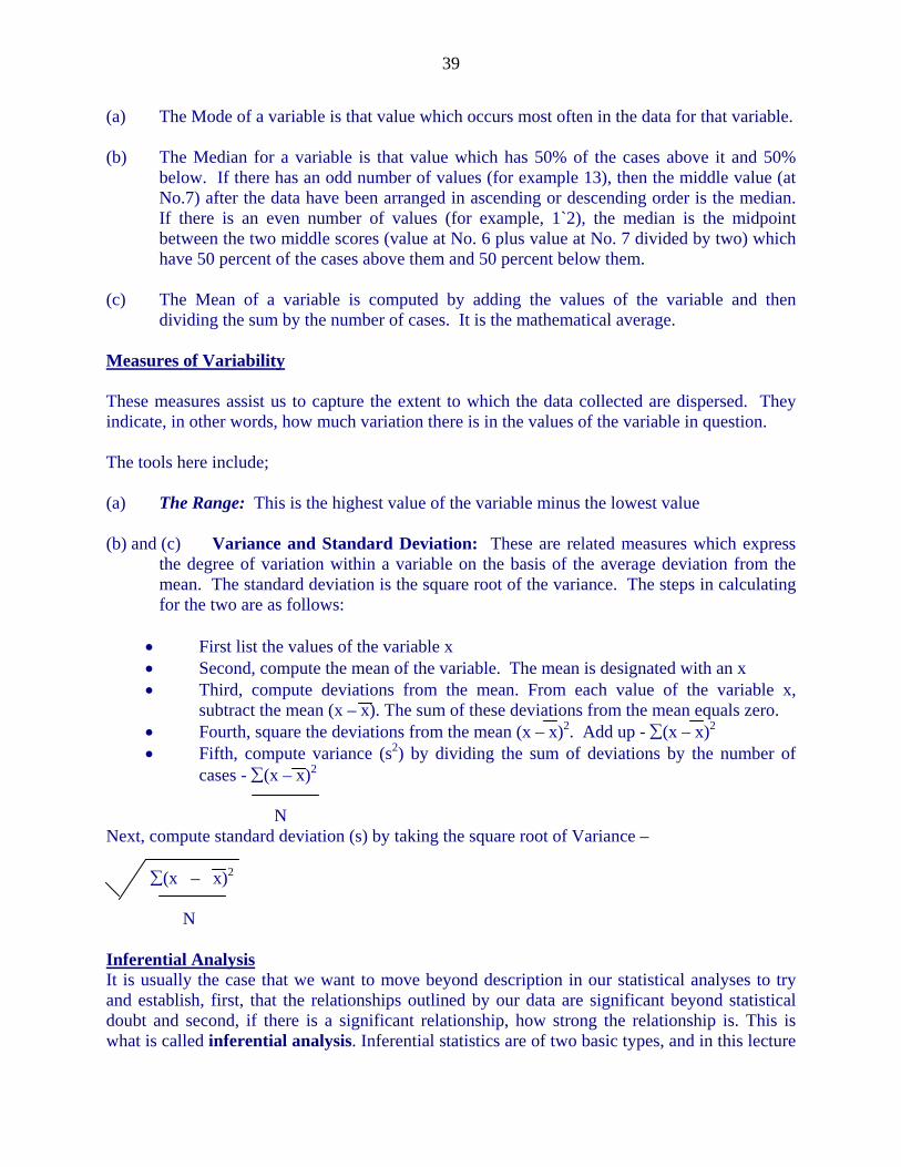
39

(a) The Mode of a variable is that value which occurs most often in the data for that variable. (b) The Median for a variable is that value which has 50% of the cases above it and 50%

below. If there has an odd number of values (for example 13), then the middle value (at No.7) after the data have been arranged in ascending or descending order is the median. If there is an even number of values (for example, 1`2), the median is the midpoint between the two middle scores (value at No. 6 plus value at No. 7 divided by two) which have 50 percent of the cases above them and 50 percent below them.

(c) The Mean of a variable is computed by adding the values of the variable and then

dividing the sum by the number of cases. It is the mathematical average. Measures of Variability These measures assist us to capture the extent to which the data collected are dispersed. They indicate, in other words, how much variation there is in the values of the variable in question. The tools here include; (a) The Range: This is the highest value of the variable minus the lowest value (b) and (c) Variance and Standard Deviation: These are related measures which express

the degree of variation within a variable on the basis of the average deviation from the mean. The standard deviation is the square root of the variance. The steps in calculating for the two are as follows:

First list the values of the variable x Second, compute the mean of the variable. The mean is designated with an x Third, compute deviations from the mean. From each value of the variable x,

subtract the mean (x – x). The sum of these deviations from the mean equals zero. Fourth, square the deviations from the mean (x – x)2. Add up - (x – x)2 Fifth, compute variance (s2) by dividing the sum of deviations by the number of

cases - (x – x)2

N Next, compute standard deviation (s) by taking the square root of Variance – (x – x)2

N Inferential Analysis It is usually the case that we want to move beyond description in our statistical analyses to try and establish, first, that the relationships outlined by our data are significant beyond statistical doubt and second, if there is a significant relationship, how strong the relationship is. This is what is called inferential analysis. Inferential statistics are of two basic types, and in this lecture

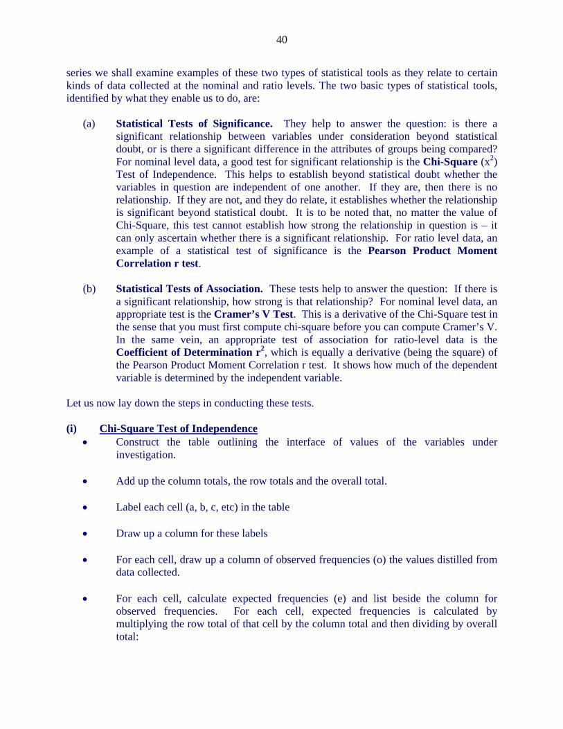
40

series we shall examine examples of these two types of statistical tools as they relate to certain kinds of data collected at the nominal and ratio levels. The two basic types of statistical tools, identified by what they enable us to do, are:

(a) Statistical Tests of Significance. They help to answer the question: is there a significant relationship between variables under consideration beyond statistical doubt, or is there a significant difference in the attributes of groups being compared? For nominal level data, a good test for significant relationship is the Chi-Square (x2) Test of Independence. This helps to establish beyond statistical doubt whether the variables in question are independent of one another. If they are, then there is no relationship. If they are not, and they do relate, it establishes whether the relationship is significant beyond statistical doubt. It is to be noted that, no matter the value of Chi-Square, this test cannot establish how strong the relationship in question is – it can only ascertain whether there is a significant relationship. For ratio level data, an example of a statistical test of significance is the Pearson Product Moment Correlation r test.

(b) Statistical Tests of Association. These tests help to answer the question: If there is

a significant relationship, how strong is that relationship? For nominal level data, an appropriate test is the Cramer’s V Test. This is a derivative of the Chi-Square test in the sense that you must first compute chi-square before you can compute Cramer’s V. In the same vein, an appropriate test of association for ratio-level data is the Coefficient of Determination r2, which is equally a derivative (being the square) of the Pearson Product Moment Correlation r test. It shows how much of the dependent variable is determined by the independent variable.

Let us now lay down the steps in conducting these tests. (i) Chi-Square Test of Independence

Construct the table outlining the interface of values of the variables under investigation.

Add up the column totals, the row totals and the overall total.

Label each cell (a, b, c, etc) in the table

Draw up a column for these labels

For each cell, draw up a column of observed frequencies (o) the values distilled from

data collected.

For each cell, calculate expected frequencies (e) and list beside the column for observed frequencies. For each cell, expected frequencies is calculated by multiplying the row total of that cell by the column total and then dividing by overall total:

41

For each cell, calculate o – e

Square the result of o – e (o – e)2 for each cell

Divide (o – e)2 by e for each cell. This is the chi-square value for each cell.

Sum up the result of (o – e)2 divided by e for all the cells. This is the computed (or calculated) Chi-Square for the entire table as expressed in the formula x2 (chi-square) = (o – e)2

e

From the Table of Critical values of Chi-square, check for critical x2 appropriate for your test. To do this, you require to first establish:

- the degree of freedom, given by number of columns in the table minus one

multiplied by number of row minus one (r – 1) (c – 1). - Level of significance, which in the social sciences is conventionally put at 0.05.

Compare calculated/computed x2 with table/critical x2. If the computed x2 is greater

than the critical x2, there is significance and the research hypothesis, to the effect that there is significant relationship between the variables under investigation, is upheld. If computed x2 is less than critical x2, then the research hypothesis is not upheld, and there is no significant relationship.

(ii) The Cramer’s V Test of Association As indicated earlier, this is a chi-square derivative and is expressed by the formula: x2 mn x2 in the formula is the computed Chi-Square value. “m” is equal to either (r – 1) or (c – 1), depending on which is less, and n is the number of cases. The resulting value of Cramer’s V will range from O, indicating no strength to the relationship, to 1, indicating extremely strong relationship. (iii) Pearson Product – Moment Correlation r Test and Coefficient of Determination r2

As indicated earlier, this is a test of significance on ratio – level data. Its definitional formula is given as r = (x – x) (y – y) (x – x)2 E (y – y)2

42

Its computational formula is given as NXY – (X) (Y) r =

[NX2 – (X)2] [NY2 – (Y)2] Steps in calculation are as follows:

List the values of x variable and sum up the values List the values of variables and sum p the values

Compute x2 and sum up the values

Compute y2 and sum up the values

Compute NY in each instance and sum up

Solve for the formula

Interpret the result. Pearson Product Moment Correlation r tests yield results ranging

from –1, indicating perfect negative relationship (the more of x, the less of y) to 0 (indicating no relationship) and +1, indicating perfect positive relationship (the more of x, the more of y).

To get coefficient of determination r2, square r. r2 specifies the extent to which the dependent variable is determined by the independent variable. Its values range from 0, indicating zero determination, to 1, indicating 100 percent determination. ORGANIZATION OF RESEARCH REPORT The way in which the research report is organized into chapters is determined by several factors, including the nature of the study (is it quantitative or qualitative, does it have extensive methodological issues to discuss or not, etc) and institutional traditions and regulations. In the case of supervised work at the Defence College, institutional factors must take precedent over other considerations. It does appear that a five-chapter format can be recommended against the background of this tradition, basically boiled down to the following: 1. Introduction 2. Literature/Theoretical Chapter 3. Methods Chapter 4. Data Analysis/Discussion Chapter 5. Conclusions/Recommendations Chapter

43

This, of course, is subject to the position and preferences of the college. Finally, participants must remember to indicate their notes and references as well as bibliography as directed by the Defence College. FURTHER READING Johnson and Joslyn, 1991: Chapters 11 – 14. Rudestam and Newton, 1992: Chapters 4 – 7.

44

V. COMPUTER APPLICATION 5.0 INTRODUCTION

SPSS (originally “Statistical Package for the Social Sciences,” now “Statistical Product and Service Solutions”) is a powerful program designed to allow users to perform a very wide range of data analysis. Data analysis is the language of research. In many fields, research is critical for human progress. Therefore, as long as there is research, there will be the need for data analysis. This guide is useful for users of SPSS versions 8, 9, 10 and 11. These four versions are similar, although there are some differences because of additional functions in the higher version. It is recommended that you use this guide whilst sitting at a computer that is running SPSS.

This guide is designed to help you analyze data on your own. A basic knowledge of statistics and a general acquaintance with the use of the computer is, however, required for this guide to be effective in guiding you on how to conduct analysis with SPSS. The type of procedure to use and what the output mean will be meaningful provided that you have at least a rudimentary knowledge of statistics. Undoubtedly, the guide should provide individuals with limited statistical background ways of using the SPSS to conduct statistical operations.

An overview of the structure of this guide follows. Firstly, data analysis is considered by introducing you to the windows and buttons you will use when analyzing your data with SPSS. Here, how to start and exit SPSS, create and save a data file and how to obtain some simple descriptive statistics are described. Secondly, crosstabulations and chi-square statistical procedure in SPSS is described. Finally, a brief overview of data management in SPSS and a step-by-step instruction on how to recode variables, add value labels, and define missing values are presented. These procedures are necessary steps to be undertaken when conducting data analysis using SPSS for Windows.

5.1 DATA ANALYSIS USING SPSS There are three basic steps involved in data analysis using the SPSS. Firstly, you must

enter the raw data and save to a file. Secondly, you must select and specify the analysis you require. Thirdly, you must examine the output produced by SPSS. These steps are illustrated below. The special windows used by SPSS to undertake these steps are described next.

45

Data Entry The data are entered into the Data Editor Window and saved to disk.

Analysis An appropriate analysis is selected and specified using the dialogue boxes.

Inspection of Results

The results of the analysis (the output) are inspected in Viewer window. An additional analysis is selected or the results are printed and reported

SPSS utilizes several different window types. However, new users of SPSS only need to be familiar with two of these windows, the Data Editor window and the Viewer window. We will be using these two windows in this guide. The other window types are explained very briefly below.

5.1.1 The Data Editor window The Data Editor window (or data window) is the window you see when you start up SPSS. This spreadsheet-like window is used to enter all the data that is going to be analyzed. You can think of this window as containing a table of all your raw data. We will examine this data in detail when SPSS started up.

5.1.2 The Viewer window

The viewer window is used to display the results of your data analysis. For this reason we will sometimes refer to it as the Output window. We will examine this window in more detail when we perform our first simple analysis.

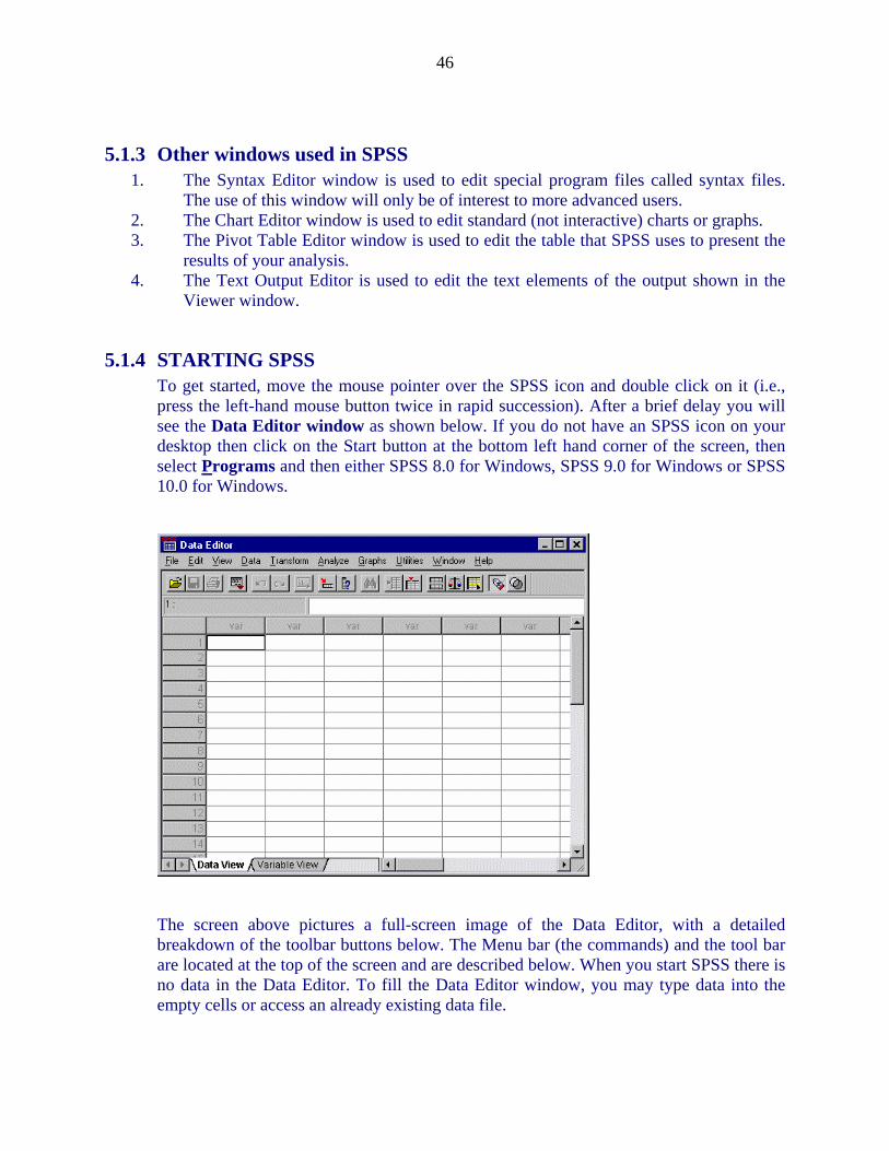
46

5.1.3 Other windows used in SPSS 1. The Syntax Editor window is used to edit special program files called syntax files.

The use of this window will only be of interest to more advanced users. 2. The Chart Editor window is used to edit standard (not interactive) charts or graphs. 3. The Pivot Table Editor window is used to edit the table that SPSS uses to present the

results of your analysis. 4. The Text Output Editor is used to edit the text elements of the output shown in the

Viewer window.

5.1.4 STARTING SPSS To get started, move the mouse pointer over the SPSS icon and double click on it (i.e., press the left-hand mouse button twice in rapid succession). After a brief delay you will see the Data Editor window as shown below. If you do not have an SPSS icon on your desktop then click on the Start button at the bottom left hand corner of the screen, then select Programs and then either SPSS 8.0 for Windows, SPSS 9.0 for Windows or SPSS 10.0 for Windows.

The screen above pictures a full-screen image of the Data Editor, with a detailed breakdown of the toolbar buttons below. The Menu bar (the commands) and the tool bar are located at the top of the screen and are described below. When you start SPSS there is no data in the Data Editor. To fill the Data Editor window, you may type data into the empty cells or access an already existing data file.

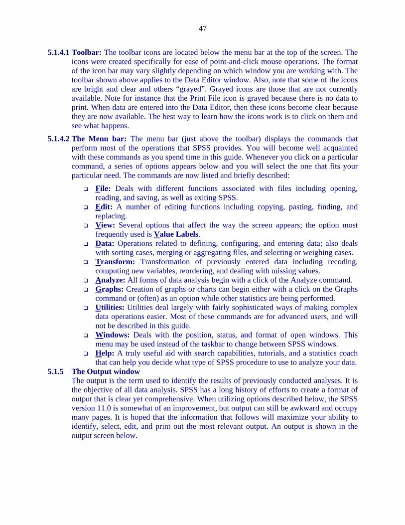
47

5.1.4.1 Toolbar: The toolbar icons are located below the menu bar at the top of the screen. The icons were created specifically for ease of point-and-click mouse operations. The format of the icon bar may vary slightly depending on which window you are working with. The toolbar shown above applies to the Data Editor window. Also, note that some of the icons are bright and clear and others “grayed”. Grayed icons are those that are not currently available. Note for instance that the Print File icon is grayed because there is no data to print. When data are entered into the Data Editor, then these icons become clear because they are now available. The best way to learn how the icons work is to click on them and see what happens.

5.1.4.2 The Menu bar: The menu bar (just above the toolbar) displays the commands that perform most of the operations that SPSS provides. You will become well acquainted with these commands as you spend time in this guide. Whenever you click on a particular command, a series of options appears below and you will select the one that fits your particular need. The commands are now listed and briefly described:

File: Deals with different functions associated with files including opening, reading, and saving, as well as exiting SPSS.

Edit: A number of editing functions including copying, pasting, finding, and replacing.

View: Several options that affect the way the screen appears; the option most frequently used is Value Labels.

Data: Operations related to defining, configuring, and entering data; also deals with sorting cases, merging or aggregating files, and selecting or weighing cases.

Transform: Transformation of previously entered data including recoding, computing new variables, reordering, and dealing with missing values.

Analyze: All forms of data analysis begin with a click of the Analyze command. Graphs: Creation of graphs or charts can begin either with a click on the Graphs

command or (often) as an option while other statistics are being performed. Utilities: Utilities deal largely with fairly sophisticated ways of making complex

data operations easier. Most of these commands are for advanced users, and will not be described in this guide.

Windows: Deals with the position, status, and format of open windows. This menu may be used instead of the taskbar to change between SPSS windows.

Help: A truly useful aid with search capabilities, tutorials, and a statistics coach that can help you decide what type of SPSS procedure to use to analyze your data.

5.1.5 The Output window The output is the term used to identify the results of previously conducted analyses. It is the objective of all data analysis. SPSS has a long history of efforts to create a format of output that is clear yet comprehensive. When utilizing options described below, the SPSS version 11.0 is somewhat of an improvement, but output can still be awkward and occupy many pages. It is hoped that the information that follows will maximize your ability to identify, select, edit, and print out the most relevant output. An output is shown in the output screen below.

48

In dealing with this screen, the objective is to edit output so that, when printed, it will be reproduced in a format most useful to you. Of course, you do not have to reorganize output before you print, but there are often advantages to doing so:

Extensive outputs will often use/waste many pages of paper. Most outputs will include some information that is unnecessary. At times a large table will be clearer if it is reorganized. You may wish to type in comments or titles for ease or clarity of interpretation.

The key element of the Output window shown above, as well as detailed description of each toolbar item follows. You will notice that several of the toolbar icons are identical to those in the SPSS Data Editor window; these buttons do the same thing that they do in the Data Editor, but with the Output instead of the Data. For example, clicking on the print icon prints the output instead of the data.

One of the most important things to learn about the SPSS Output window is the use of the outline view on the left of the screen. On the right side of the window is the output from the SPSS procedures that were run, and on the left is the outline (like a table of contents without page numbers) of the output. The SPSS output is actually composed of a series of output objects; these objects may be titles (e.g., “Frequencies”), tables of numbers, or charts, among other things. Each of these objects is listed in the outline view:

49

Note: You will notice that there is no “notes” section in the output window to correspond with the “notes” title in the outline view. That’s because the notes are (by default) hidden. If you want to see the notes, just double click on the closed book icon to the right of the notes title. The closed book icon will then become an open-book icon and the notes will materialize in the window to the right. The outline view makes navigating the output easier. If you want to move to the Crosstabs output, for example, you merely need to click on the word “Crosstabs” in the outline view, and the crosstabs will appear in the output window. If you want to delete the Descriptives section (perhaps because you selected an incorrect variable), simply click on the word “Descriptives” and select menu item Edit then click Delete. If you want to move some output from one section to another (to re-arrange the order), you can select an output object (or a group of output objects), and select Edit then click Cut. After that, select another output object below which you want to place the output object(s) you have cut, select Edit then click Paste After. If you have been working with the same data for a while, you may produce a lot of output. So much output may be produced, in fact, that it becomes difficult to navigate throughout the output even with the outline view. To help with this problem, you can “collapse” a group of output objects underneath a heading. To do this, click on the minus sign to the left of the heading. One particularly useful command when you are working with output is the insert text command. When you click on this button, an SPSS Text object is inserted. In this box,

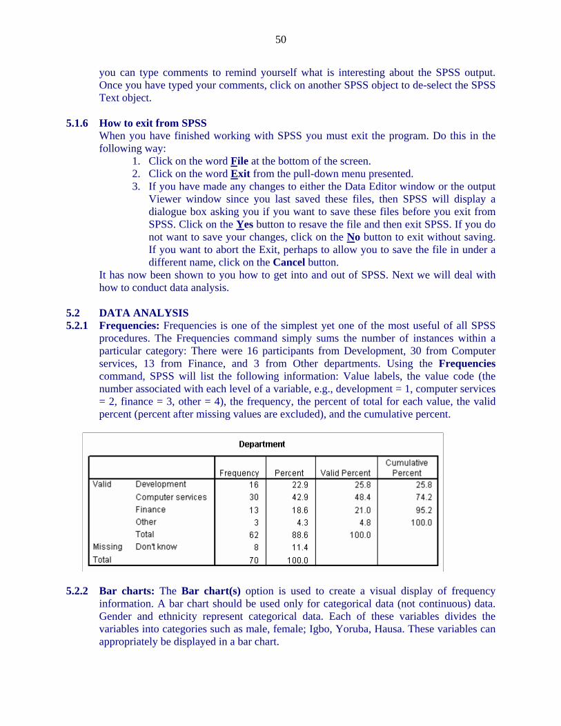
50

you can type comments to remind yourself what is interesting about the SPSS output. Once you have typed your comments, click on another SPSS object to de-select the SPSS Text object.

5.1.6 How to exit from SPSS When you have finished working with SPSS you must exit the program. Do this in the following way:

1. Click on the word File at the bottom of the screen. 2. Click on the word Exit from the pull-down menu presented. 3. If you have made any changes to either the Data Editor window or the output

Viewer window since you last saved these files, then SPSS will display a dialogue box asking you if you want to save these files before you exit from SPSS. Click on the Yes button to resave the file and then exit SPSS. If you do not want to save your changes, click on the No button to exit without saving. If you want to abort the Exit, perhaps to allow you to save the file in under a different name, click on the Cancel button.

It has now been shown to you how to get into and out of SPSS. Next we will deal with how to conduct data analysis.

5.2 DATA ANALYSIS 5.2.1 Frequencies: Frequencies is one of the simplest yet one of the most useful of all SPSS

procedures. The Frequencies command simply sums the number of instances within a particular category: There were 16 participants from Development, 30 from Computer services, 13 from Finance, and 3 from Other departments. Using the Frequencies command, SPSS will list the following information: Value labels, the value code (the number associated with each level of a variable, e.g., development = 1, computer services = 2, finance = 3, other = 4), the frequency, the percent of total for each value, the valid percent (percent after missing values are excluded), and the cumulative percent.

5.2.2 Bar charts: The Bar chart(s) option is used to create a visual display of frequency information. A bar chart should be used only for categorical data (not continuous) data. Gender and ethnicity represent categorical data. Each of these variables divides the variables into categories such as male, female; Igbo, Yoruba, Hausa. These variables can appropriately be displayed in a bar chart.

51

Continuous data containing series of numbers or values such as total points, weight in pounds, age, and so forth. Continuous variables are typically represented in Histogram.

5.2.3 Histograms: For continuous data, the Histogram(s) option will create appropriate visual display. A histogram is used to indicate frequencies of a range of values. A histogram is used when the number of instances of a variable is too large to want to list all of them. A good example is the age of workers in a factory. Since it would be too cumbersome to list all ages on a graph, it is more practical to list the number of workers within a range of values, such as how many workers are between 40 and 49 years, between 50 and 59 years, and so forth.

5.2.4 To obtain a Frequency output in SPSS:

1. Once your data is entered, checked and saved click on the word Analyze at the top of the screen.

2. Select (click on) Descriptive Statistics.

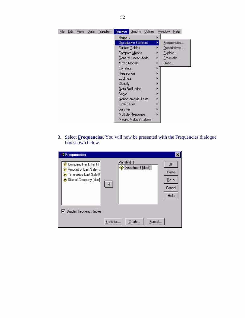
52

3. Select Frequencies. You will now be presented with the Frequencies dialogue

box shown below.

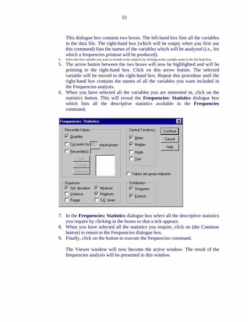
53

This dialogue box contains two boxes. The left-hand box lists all the variables

in the data file. The right-hand box (which will be empty when you first use this command) lists the names of the variables which will be analyzed (i.e., for which a frequencies printout will be produced).

4. Select the first variable you want to include in the analysis by clicking on the variable name in the left-hand box.

5. The arrow button between the two boxes will now be highlighted and will be pointing to the right-hand box. Click on this arrow button. The selected variable will be moved to the right-hand box. Repeat this procedure until the right-hand box contains the names of all the variables you want included in the Frequencies analysis.

6. When you have selected all the variables you are interested in, click on the statistics button. This will reveal the Frequencies: Statistics dialogue box which lists all the descriptive statistics available in the Frequencies command.

7. In the Frequencies: Statistics dialogue box select all the descriptive statistics

you require by clicking in the boxes so that a tick appears. 8. When you have selected all the statistics you require, click on (the Continue

button) to return to the Frequencies dialogue box. 9. Finally, click on the button to execute the frequencies command.

The Viewer window will now become the active window. The result of the frequencies analysis will be presented in this window.

54

5.2.5 To obtain a Tables output in SPSS:

1. On the menu bar, click on the word Analyze. 2. Click on Custom Tables. 3. Click on Basic Tables. This will display the Basic Tables dialogue box. 4. Click on the name of the variable you require summary descriptive statistics,

then click on the arrow button next to the Summaries box to move the variable into the Summaries box.

5. Next click on the name of the grouping variable. The grouping variable will be used to create the two or more groups for which the descriptive statistics will be calculated.

6. Now click on the arrow next to either the Down, the Across or the Separate Tables boxes. Which of these you choose determines how the table will appear in the output. The Down option produces a separate row for each level of the grouping variable, whereas the Across options produces a separate column for each level of the grouping variable. The Separate Tables option produces a separate table for each level of the grouping variable. Experiment with this settings to see which suit you best.

7. Now click on the Statistics button. The Basic Tables: Statistics dialogue box will appear.

8. Select the descriptive statistics you require by picking them from the list in the left of the dialogue box. Click on the Add button. To add the selected statistics to the box marked Cell Statistics. You may need to scroll down through the list of statistics available to find all of those you require.

9. Once the required statistics have been selected, click on the Continue button. This will return you to the Basic Tables dialogue box. Now click on the OK button. The tables of statistics requested will now appear in the Viewer window.

5.2.6 Descriptives Descriptive is another frequently used SPSS procedure. Descriptive statistics are designed to give you information about the distributions of your variables. Within this broad category are measures of central tendency (Mean, Median, Mode), measures of variability around the mean (Std deviation and Variance), measures of deviation from normality (Skewness and Kurtosis), information concerning the spread of the distribution (Maximum, Minimum, and Range), and information about the stability or sampling error of certain measures including standard error (S.E.) of the mean (S.E. mean). Using the Descriptives command, it is possible to access all of these statistics or any subset of them.

Whether first entering SPSS or returning from earlier operations the standard menu of commands across the top is required. As long as it is visible you may perform any analysis as long as you have data in the Data Editor. It is not necessary for the data window to be visible.

5.2.6.1 To obtain Descriptives output in SPSS:

55

1. Once your data is entered, checked and saved click on the word Analyze at the top of the screen.

2. Select (click on) Descriptive Statistics. 3. Select Descriptives. You will now be presented with the Descriptives

dialogue box. 4. Click the desired variable name in the box to the left and then pasting it into

the Variable(s) box to the right by clicking the right arrow in the middle of the screen. To deselect a variable (i.e., to move it from the Variable(s) box back to the original list), click on the variable in the active box and the front arrow in the center will become a back arrow. Click on the left arrow to move the variable back. To clear all the variables from the active box, click the Reset button.

5. If you wish to calculate more than the four default statistics, after selecting the desired variables, before clicking the OK, it is necessary to click the Options button. To select the desired descriptive statistics, the procedure is simply to click the box behind the desired value of the descriptive statistics you wish. This is followed by a click of Continue and OK.

Crosstabulation and Chi-square Analyses

The purpose of crosstabulation is to show in tabular format the relationship between two or more categorical variables. Categorical variables include those in which distinct categories exist such as gender (female, male), ethnicity (Igbo, Yoruba, Hausa), place of residence (urban, rural), responses (yes, no), and many more. Crosstabulation can be used with continuous data only if such data are divided into separate categories, such as age (0-19 years, 20-39 years, 40-59 years, 60-79 years, 80-99 years), total points (0-99, 100-149, 150-199, 200-250), and so on. While it is acceptable to perform crosstabulation with continuous data that has been categorized, it is rare to perform chi-square analyses with continuous data because a great deal of useful information about the distribution is lost by the process of categorization. Nonetheless, crosstabulation with continuous data is often used for purposes of data description and display. The SPSS command Crosstabs and the subcommands Cells and Statistics are used to access all necessary information about comparisons of frequency data.

In addition to frequencies (or the observed values) within each cell, SPSS can also compute the expect6ed value for each cell. Expected value is based on the assumption that the two variables are independent of each other. The purpose of a chi-square test is to determine whether the observed values for the cells deviate significantly from the corresponding expected values for those cells. If there is a large discrepancy between the observed values and the expected values, the X2 statistic would be large, suggesting a significant difference between observed and expected values. Along with this statistic, a probability value is computed. With P < .05, it is commonly accepted that the observed values differ significantly from the expected values and that the two variables are not independent of each other.

5.2.7.1 To Perform the Chi-square Test:

56

1. Click on the menu item Analyze. 2. Click on the words Descriptive Statistics. 3. Now click on the Crosstabs.

4. Select the name of the variable that you want to form the row of your contingency table and then click the arrow button to move it to the Row(s) box.

5. Now repeat this procedure to move your column variable into the Column(s) box.

6. Now click on the Statistics button; this will bring up the Crosstabs: Statistics dialogue box. Click (check) Chi-square and then click Continue.

57

7. In the main Crosstabs dialog box, click on the Cells button – this brings up the Crosstabs: Cell Display dialogue box.

8. Click on the display options you want. These options control the information included in the contingency table. It is recommended that you select both of the Counts options and all 3 Percentages options.

9. Click on the Continue button to return to the Crosstabs dialogue box. 10. Finally, click on OK button in the Crosstabs dialogue box. SPSS will now

switch to the Output window and display the contingency table and the chi-square results.

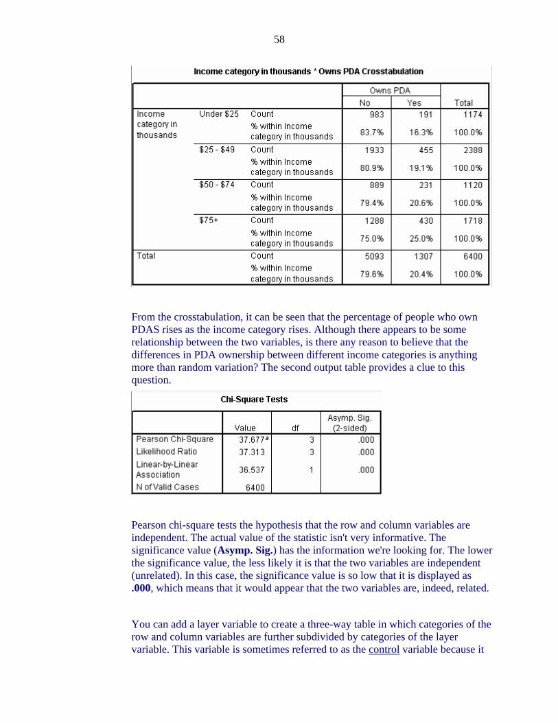
58

From the crosstabulation, it can be seen that the percentage of people who own PDAS rises as the income category rises. Although there appears to be some relationship between the two variables, is there any reason to believe that the differences in PDA ownership between different income categories is anything more than random variation? The second output table provides a clue to this question.

Pearson chi-square tests the hypothesis that the row and column variables are independent. The actual value of the statistic isn't very informative. The significance value (Asymp. Sig.) has the information we're looking for. The lower the significance value, the less likely it is that the two variables are independent (unrelated). In this case, the significance value is so low that it is displayed as .000, which means that it would appear that the two variables are, indeed, related.

You can add a layer variable to create a three-way table in which categories of the row and column variables are further subdivided by categories of the layer variable. This variable is sometimes referred to as the control variable because it

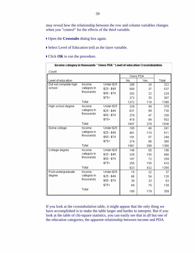
59

may reveal how the relationship between the row and column variables changes when you "control" for the effects of the third variable.

Open the Crosstabs dialog box again.

Select Level of Education (ed) as the layer variable.

Click OK to run the procedure.

If you look at the crosstabulation table, it might appear that the only thing we have accomplished is to make the table larger and harder to interpret. But if you look at the table of chi-square statistics, you can easily see that in all but one of the education categories, the apparent relationship between income and PDA

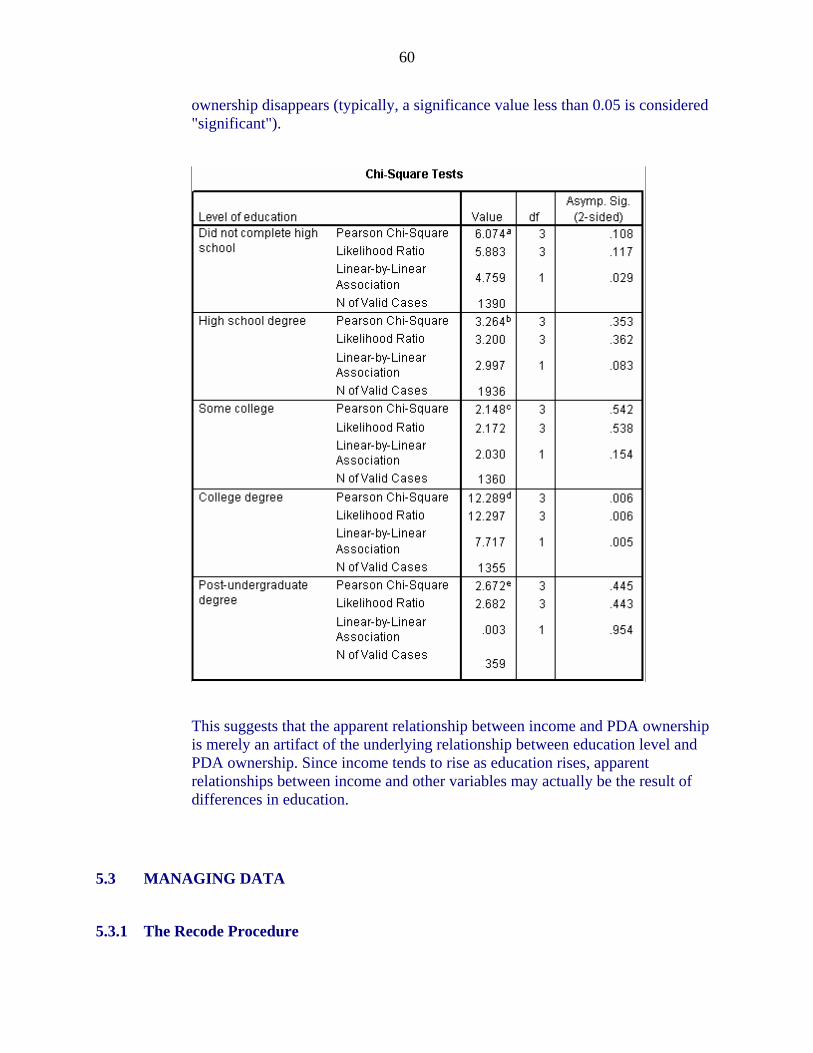
60

ownership disappears (typically, a significance value less than 0.05 is considered "significant").

This suggests that the apparent relationship between income and PDA ownership is merely an artifact of the underlying relationship between education level and PDA ownership. Since income tends to rise as education rises, apparent relationships between income and other variables may actually be the result of differences in education.

5.3 MANAGING DATA

5.3.1 The Recode Procedure

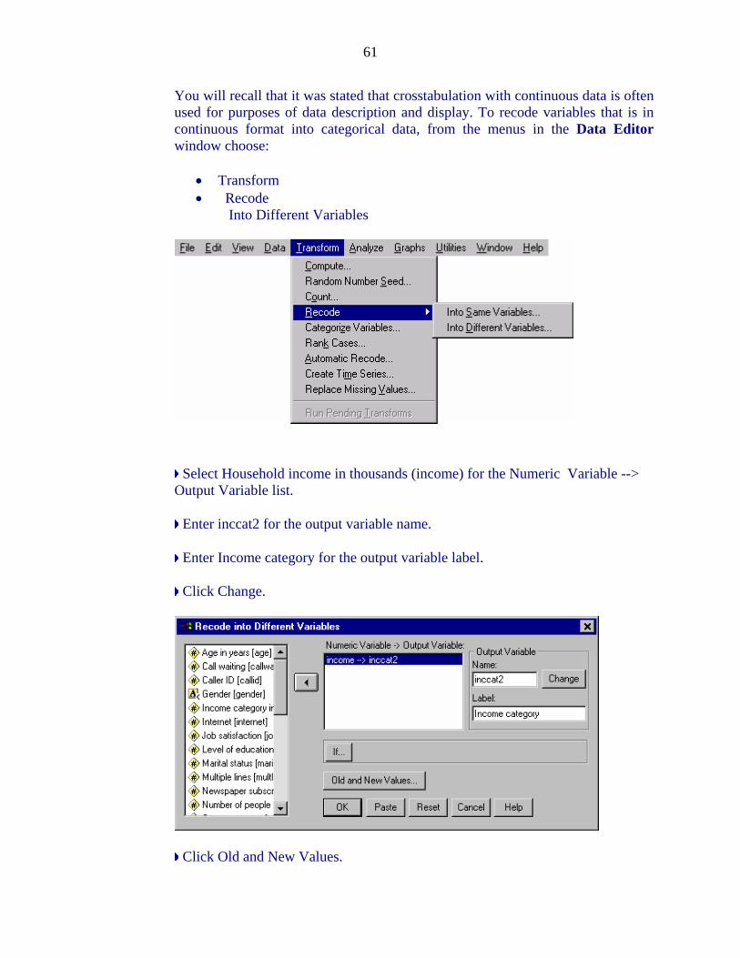
61

You will recall that it was stated that crosstabulation with continuous data is often used for purposes of data description and display. To recode variables that is in continuous format into categorical data, from the menus in the Data Editor window choose:

Transform Recode

Into Different Variables

Select Household income in thousands (income) for the Numeric Variable --> Output Variable list.

Enter inccat2 for the output variable name.

Enter Income category for the output variable label.

Click Change.

Click Old and New Values.

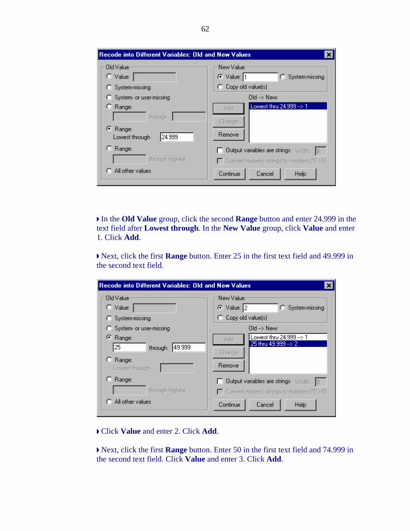
62

In the Old Value group, click the second Range button and enter 24.999 in the text field after Lowest through. In the New Value group, click Value and enter 1. Click Add.

Next, click the first Range button. Enter 25 in the first text field and 49.999 in the second text field.

Click Value and enter 2. Click Add.

Next, click the first Range button. Enter 50 in the first text field and 74.999 in the second text field. Click Value and enter 3. Click Add.

63

Next, click the third Range button. Enter 75 in the text field before through highest. Click Value and enter 4. Click Add. Click Continue, and then click OK in the main dialog box.

The new variable is displayed in the Data Editor. Since the variable is added to the end of the file, it is displayed in the far right column in Data view and in the last row in Variable view.

64

When you create a new variable based on the recoded values of another variable, there are two basic rules you should follow. The recoded categories should be:

Mutually exclusive. There shouldn't be any overlap in category definitions. For example, the categories 25-50 and 50-75 are not mutually exclusive, since both categories contain the value 50.

Exhaustive. There should be appropriate categories for all values of the original variable. For example, the categories 25-49 and 50-74 would not include values that might fall between 49 and 50.

Although all the income values in the demo.sav data file appear to be integers, just to be on the safe side we used the categories 25-49.999 and 50-74.999 to make sure none of values were left out.

65

5.3.2 Value Labels

At this point, you might want to add value labels that describe what each of the four categorical values represents. Value labels provide a method for mapping your variable values to a string label. For example, there are two acceptable values for the marital variable. A value of 0 means that the subject is single, and a 1 means that he or she is married.

In the Data Editor, click the Variable view located on the left hand corner of the bottom of your screen. The Variable view of the Data Editor now appears.

1. Select the Values cell for the marital row and click the button to open the Value Labels dialog box.

66

The Value is the actual numeric value. The Value Label is the string label applied to the specified numeric value.

2. Type 0 in the Value field. Type Single for the Value Label. 3. Click Add to have this label added to the list. Repeat the process, this

time entering 1 for the Value and Married for the Value Label.

4. Click OK to implement the changes and return to the Data Editor.

These labels can also be displayed in the Data View, which can help to make your data more readable. Click the Data View tab at the bottom of the Data Editor window. From the menus choose:

View Value Labels

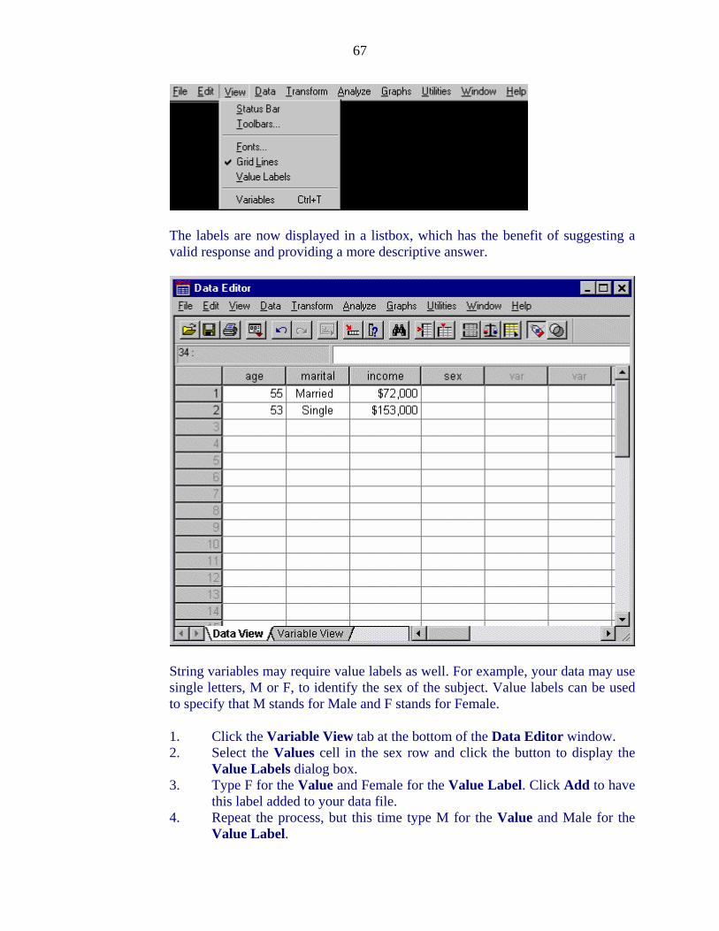
67

The labels are now displayed in a listbox, which has the benefit of suggesting a valid response and providing a more descriptive answer.

String variables may require value labels as well. For example, your data may use single letters, M or F, to identify the sex of the subject. Value labels can be used to specify that M stands for Male and F stands for Female.

1. Click the Variable View tab at the bottom of the Data Editor window. 2. Select the Values cell in the sex row and click the button to display the

Value Labels dialog box. 3. Type F for the Value and Female for the Value Label. Click Add to have

this label added to your data file. 4. Repeat the process, but this time type M for the Value and Male for the

Value Label.

68

5. Click OK to implement your changes and return to the Variable View.

Because string values are case sensitive, you should make sure you are consistent with your cases. A lower case m is not the same as a capital M. In a previous example, we chose to have value labels displayed rather than the actual data by selecting Value Labels from the View menu. You can use these values for data entry.

1. Click the Data View to view the data. In the first row, select the cell for sex and select Male from the list.

2. In the second row, set the respondent's sex to Female. Only defined values are listed, which helps to ensure that the data entered is in a format you expect.

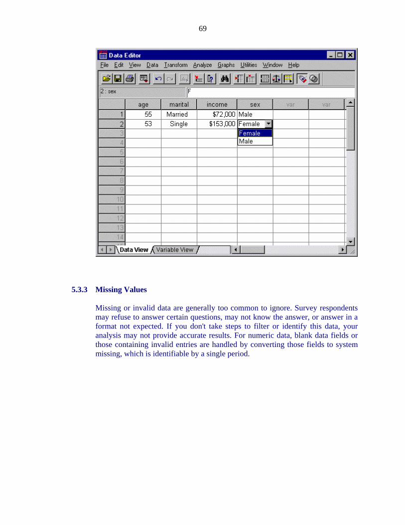
69

5.3.3 Missing Values

Missing or invalid data are generally too common to ignore. Survey respondents may refuse to answer certain questions, may not know the answer, or answer in a format not expected. If you don't take steps to filter or identify this data, your analysis may not provide accurate results. For numeric data, blank data fields or those containing invalid entries are handled by converting those fields to system missing, which is identifiable by a single period.

70

The reason a value is missing may be important to your analysis. For example, you may find it useful to distinguish between those who refused to answer a question, and those who didn't answer a question because it was not applicable to them.

1. Click the Variable View tab at the bottom of the Data Editor window. 2. Select the Missing cell in the Age row and click the button to open the

Missing Values dialog box.

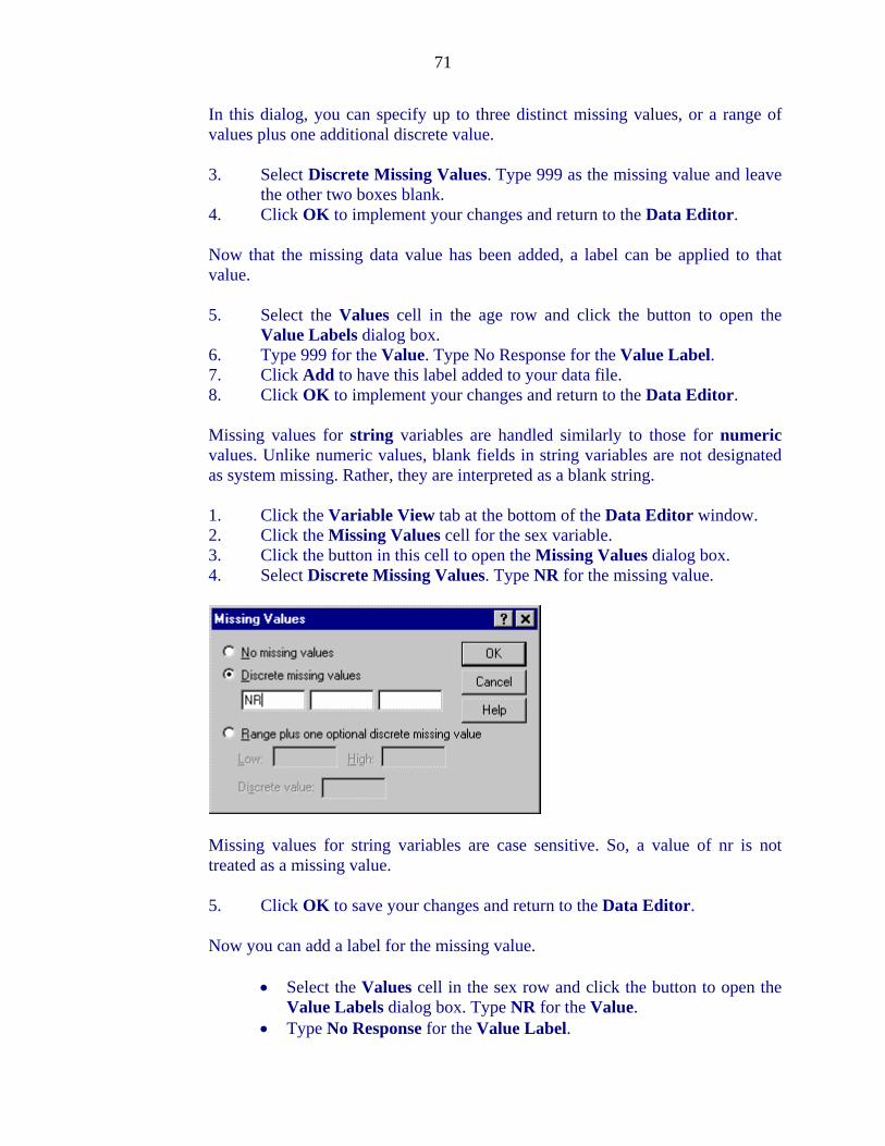
71

In this dialog, you can specify up to three distinct missing values, or a range of values plus one additional discrete value.

3. Select Discrete Missing Values. Type 999 as the missing value and leave the other two boxes blank.

4. Click OK to implement your changes and return to the Data Editor.

Now that the missing data value has been added, a label can be applied to that value.

5. Select the Values cell in the age row and click the button to open the Value Labels dialog box.

6. Type 999 for the Value. Type No Response for the Value Label. 7. Click Add to have this label added to your data file. 8. Click OK to implement your changes and return to the Data Editor.

Missing values for string variables are handled similarly to those for numeric values. Unlike numeric values, blank fields in string variables are not designated as system missing. Rather, they are interpreted as a blank string.

1. Click the Variable View tab at the bottom of the Data Editor window. 2. Click the Missing Values cell for the sex variable. 3. Click the button in this cell to open the Missing Values dialog box. 4. Select Discrete Missing Values. Type NR for the missing value.

Missing values for string variables are case sensitive. So, a value of nr is not treated as a missing value.

5. Click OK to save your changes and return to the Data Editor.

Now you can add a label for the missing value.

Select the Values cell in the sex row and click the button to open the Value Labels dialog box. Type NR for the Value.

Type No Response for the Value Label.

72

Click Add to have this label added to your project. Click OK to implement your changes and return to the Data Editor.

Once you've defined variable attributes for a variable, you can copy those attributes and apply them to other variables.

In the Variable View, type agewed in the first cell of the first blank row. Type Age Married in the Label column. Click the Values cell in the age row. From the menus choose: Edit; Copy

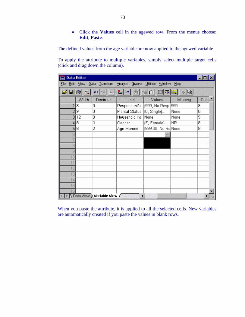
73

Click the Values cell in the agewed row. From the menus choose: Edit; Paste.

The defined values from the age variable are now applied to the agewed variable.

To apply the attribute to multiple variables, simply select multiple target cells (click and drag down the column).

When you paste the attribute, it is applied to all the selected cells. New variables are automatically created if you paste the values in blank rows.

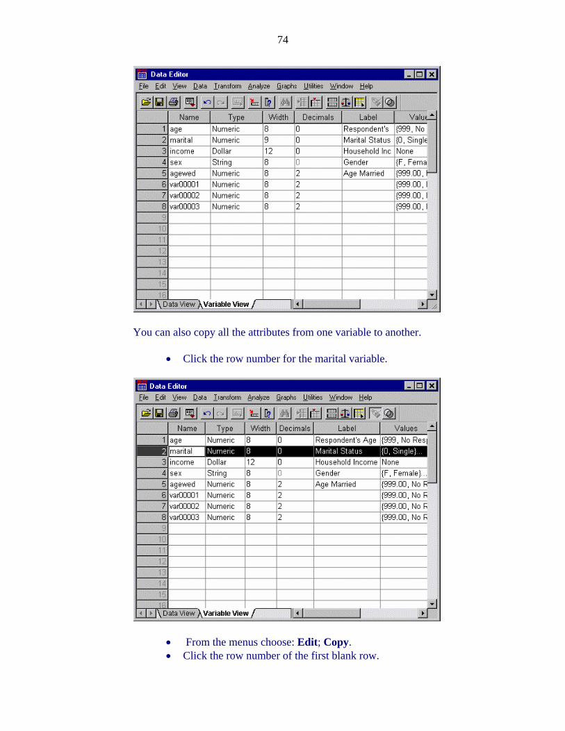
74

You can also copy all the attributes from one variable to another.

Click the row number for the marital variable.

From the menus choose: Edit; Copy. Click the row number of the first blank row.

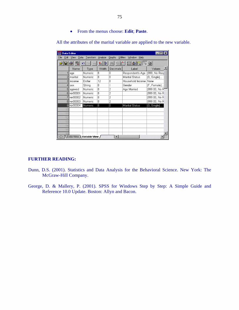
75

From the menus choose: Edit; Paste.

All the attributes of the marital variable are applied to the new variable.

FURTHER READING:

Dunn, D.S. (2001). Statistics and Data Analysis for the Behavioral Science. New York: The McGraw-Hill Company.

George, D. & Mallery, P. (2001). SPSS for Windows Step by Step: A Simple Guide and Reference 10.0 Update. Boston: Allyn and Bacon.

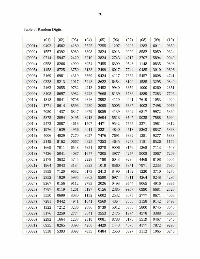
76

Table of Random Digits.

(01) (02) (03) (04) (05) (06) (07) (08) (09) (10)

(0001) 9492 4562 4180 5525 7255 1297 9296 1283 6011 0350

(0002) 1557 0392 8989 6898 3824 6013 0020 8582 5059 9324

(0003) 0714 5947 2420 6210 3824 2743 4217 3707 5894 0040

(0004) 0558 8266 4990 8954 7455 6309 9543 1148 0835 0808

(0005) 1458 8725 3750 3138 2499 6017 7744 0485 3010 9606

(0006) 5169 6981 4319 3369 9424 4117 7632 5457 0608 4741

(0007) 0328 5213 1017 5248 8622 6454 8120 4585 3295 0840

(0008) 2462 2055 9782 4213 3452 9940 8859 1000 6260 2851

(0009) 8408 8697 3982 8228 7668 8139 3736 4889 7283 7706

(0010) 1818 5041 9706 4646 3992 4110 4091 7619 1053 4020

(0011) 1771 8614 8593 0930 2095 5005 6387 4002 7498 0066

(0012) 7050 1437 6847 4679 9059 4139 6602 6817 9972 5360

(0013) 5875 2094 0495 3213 5694 5513 3547 9035 7588 5994

(0014) 2473 2087 4618 1507 4471 9542 7565 2371 3981 0812

(0015) 1976 1639 4956 9011 8221 4840 4513 5263 8837 5868

(0016) 4006 4029 7270 8027 7476 7691 6362 1251 9277 5833

(0017) 2149 8162 0667 0825 7353 4645 3273 1181 8526 1176

(0018) 1669 7011 6548 5851 8278 9006 8176 1268 7113 4548

(0019) 7436 5041 4087 1647 7205 3977 4257 9008 3067 7206

(0020) 2178 3632 5745 2228 1780 6043 9296 4469 8108 5005

(0021) 1964 3043 3134 8923 1019 8560 5871 7971 2233 7960

(0022) 5859 7120 9682 0173 2413 8490 6162 1220 3710 5270

(0023) 2352 1929 5985 3303 9590 6974 5811 4264 0248 4295

(0024) 9267 0156 9112 2783 2026 0493 9544 8065 4916 3835

(0025) 4787 0119 1261 5197 0156 2385 9957 0990 6681 2323

(0026) 5550 0699 8080 1152 6002 2532 3075 2777 8671 4068

(0027) 7281 9442 4941 1041 0569 4354 8000 3158 9142 5498

(0028) 1322 7212 3286 2886 9739 5012 0360 5800 9745 8640

(0029) 5176 2259 2774 3641 3553 2475 1974 4578 3388 6656

(0030) 2292 1664 1237 2518 0081 8788 8170 5519 0467 4646

(0031) 6935 8265 3393 4268 4429 1443 4670 4177 7872 9298

(0032) 8538 5393 8093 7835 0484 2550 0827 3112 1065 0246

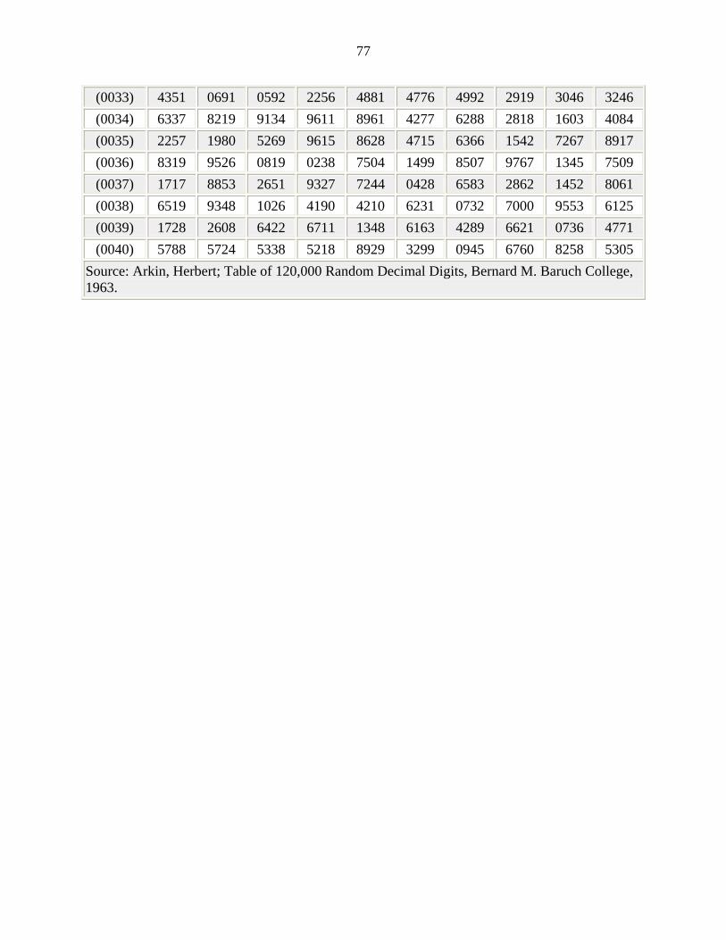
77

(0033) 4351 0691 0592 2256 4881 4776 4992 2919 3046 3246

(0034) 6337 8219 9134 9611 8961 4277 6288 2818 1603 4084

(0035) 2257 1980 5269 9615 8628 4715 6366 1542 7267 8917

(0036) 8319 9526 0819 0238 7504 1499 8507 9767 1345 7509

(0037) 1717 8853 2651 9327 7244 0428 6583 2862 1452 8061

(0038) 6519 9348 1026 4190 4210 6231 0732 7000 9553 6125

(0039) 1728 2608 6422 6711 1348 6163 4289 6621 0736 4771

(0040) 5788 5724 5338 5218 8929 3299 0945 6760 8258 5305

Source: Arkin, Herbert; Table of 120,000 Random Decimal Digits, Bernard M. Baruch College, 1963.