Introduction to Turbulence by

Håkan Gustavsson

Division of Fluid Mechanics

Luleå University of Technology

Foreword

The intention with these pages is to present the student with the basic theoretical concepts of

turbulence and derive exact relations from the governing equations. The idea is to show that

despite the complexity of turbulent flows, some general properties can be educed from the

equations. Hopefully, this will remove some of the mystique that has surrounded turbulence

as a topic in undergraduate courses. The material is used as lecture notes in the course MTM

162 (Advanced Fluid Mechanics) given in the last year of undergraduate studies at Ltu.

Luleå,

October 2006

Håkan Gustavsson

Division of Fluid Mechanics

Contents Page

1. Introduction 1

2. Reynolds’ decomposition 3

3. Equations for the mean flow 4

3.1 Continuity 4

3.2 Momentum 4

3.3 Kinetic energy 6

4. Equations for the turbulent fluctuations 7

4.1 Momentum 7

4.2 Kinetic energy 8

5. Turbulent channel flow 9

5.1 Momentum equation 9

5.2 Turbulence production 13

5.3 Mean velocity profile 14

6. Kolmogorov microscales 16

7. Turbulence structure 17

References 18

1

1. Introduction

Turbulence is generally considered one of the unresolved phenomena of physics. This means

that there is not one model that describes the appearance and maintenance of turbulence in all

situations where it appears. Because of the technical importance of turbulence, models based

on correlations of particular experimental data have been developed to a large extent.

The task to develop a general turbulence model is challenging since turbulence appears almost

everywhere: Flows in rivers, oceans and the atmosphere are large scale examples. Flows in

pipes, pumps, turbines, combustion processes, in the wake of cars, airplanes and trains are

some technical examples. Even the blood flow in the aorta is occasionally turbulent. In fact,

one can say that turbulence is the general flow type on medium and large scales whereas

laminar flows appear on small scales, and where the viscosity is high. For example, the flow

of lubricating oils in bearings is laminar.

Before we discuss the technical aspects of turbulence it is necessary to state its main

kinematic characteristics. In the list below, some flows may have one or two features but

turbulence has all three.

Irregularity. Observing structures in the flow from a smoke stack, or measuring the velocity

in a pipe flow, show that any particular pattern never repeats itself. This randomness suggests

that a statistical treatment of turbulence is worthwhile. In fact, statistical quantities such as

mean values, correlations etc. are generally repeatable and make statistical theories attractive.

Mixing. A case of randomness is the deflection of a water surface due to wind. However, in

this flow fluid particles stay largely in one place which they do not in a stirred cup of coffee.

Thus, mixing is a prominent feature of turbulence and involves mixing of particles and all

physical quantities related to particles i.e. heat, momentum etc.

Three-dimensional vorticity fluctuations. Turbulent flows always exhibit high levels of

vorticity. The maintenance of turbulence requires the process of vortex stretching which

occurs only in 3D. A word of caution: 2D turbulence may occur if magnetic fields control the

flow.

In addition to these kinematic characteristics, we may also add some features of turbulence

that help to decide when to expect its appearance and judge its physical significance.

2

Large Reynolds number. Typical for all turbulent flows is that a relevant Reynolds number

(UL/ν) for the flow is large. It is the objective for stability theory to determine the critical

Reynolds number over which turbulence may appear. This is a part of the turbulence enigma.

Dissipation. Turbulent flows loose mechanical energy due to the action of shear stresses

(dissipation) at a much larger rate than laminar flows. The flow losses are much larger. The

energy is converted into internal energy and thus shows up as an increase of temperature.

Without a continuous supply of energy, turbulence decays (cf. the stirred coffee in a cup when

the spoon is removed).

Continuum. The smallest scales of turbulence are generally far larger than molecular length

scales. Turbulence is therefore a continuum phenomenon, and should be possible to describe

by the equations of motion of fluid mechanics.

Turbulent flows are flows. Turbulence is a feature of the flow and not of the fluid. Thus,

different fluids show the same properties given the (non-dimensional) flow parameters are the

same.

For the analysis of turbulence phenomena we use the equations of motion (continuity,

momentum and energy) but the added complexity of randomness makes statistical tools

necessary. Mathematically, we will make frequent use of tensor notation in writing the

equations of motion. This simplifies the derivations and reduces the writing considerably. A

powerful tool is also dimensional analysis which relates the ingredient variables through their

dimensions. With simple assumptions about the flow very far-reaching conclusions can be

drawn with dimensional arguments. We will use this technique mainly when deriving the

smallest dissipative scales in turbulence, the Kolmogorov microscales.

In choosing specific flows to analyse, we pick wall bounded turbulent flows (channel flow)

for which analytical results may be derived and some crucial concepts appear. The next step

would be to treat ‘free’ turbulence (wakes, jets and free shear layers) where just a modest

level of turbulence modelling (eddy viscosity) leads to surprisingly useful results. The further

steps of turbulence modelling and the modern approach of direct numerical simulation of

turbulence (DNS) are treated at the graduate level.

3

2. Reynolds’ decomposition

Typical signals from measurements of velocity components near a solid wall are shown in

figure 2.1. The data illustrate the randomness of the signal but one can generally produce a

Figure 2.1: Near-wall data of u- v- and uv signals and the corresponding short-time variances

of u and v for T=10t*.(From Alfredsson & Johansson 1984, JFM 139)

time-average defined as

∫∞→

==T

0Tdt)t(f

T1limFf , (2.1)

where f can be any of the fluid mechanical variables of interest (velocity component, pressure

etc.). We use the over-bar notation, or capital letter, for the time-average. Using this

definition, we split each instantaneous component into its time-average and a time-dependent

fluctuation. For the velocity and the pressure this gives

ui = Ui + ui′ (Note that ,0ui =′ by definition)

p = P + p′ (2.2a,b)

This splitting of a turbulent signal is denoted Reynolds′ decomposition of a turbulent flow.

4

3. Equations for the mean flow

To describe the average and dynamic properties of turbulent flows, use is made of the basic

conservation laws of fluid mechanics, i.e. the equations for mass, momentum and energy.

These relations have in general to be complemented with a state condition for the fluid.

In this text we will not treat energy through the thermodynamic energy equation but restrict

the study to the kinetic energy. This can be done without invoking thermodynamics but rather

by multiplying the momentum equation with a suitable velocity component.

3.1 Continuity

In this presentation we will assume the flow to be incompressible i.e.

div u = ui,i = 0 (3.1)

Using the decomposition in (2.2a), it is deduced that the following relations apply for the

mean flow and the fluctuations:

Ui,i = 0 (3.2)

and u′i,i = 0 (3.3)

Thus, both the mean flow and the fluctuations satisfy the incompressible condition.

3.2 Momentum

We first formulate the averaging process for the general momentum equation and then

specialize to the Navier-Stokes equations. Thus, we have

j

iji

j

ij

ii

xF

xuu

tu

DtDu

∂σ∂

+ρ=⎟⎟⎠

⎞⎜⎜⎝

⎛

∂∂

+∂∂

ρ=ρ (3.4)

where Fi is a mass force (typically g) and σij is the stress tensor.

Using the decomposition in (2.2a) for ui and applying the averaging process (2.1) the left hand

side of (3.4) becomes

⎟⎟⎠

⎞⎜⎜⎝

⎛

∂′∂′+

∂∂

=∂

′+∂′+=∂∂

j

ij

j

ij

j

iijj

j

ij x

uuxUUρ

x)u(U)u (Uρ

xuuρ (3.5)

In the averaging process, the two terms involving only one primed quantity become zero so

only the mean term and the doubly primed term remain. Using continuity, the last term can

also be written as

j

ji

j

ij x

)uuρ(xuuρ

∂

′′∂=

∂′∂′ (3.6)

5

For the stress tensor we haveijijij σ′+Σ=σ , where Σ is the time-average. The average of the

fluctuating part depends on the particular (rheological) model that is used to describe the

relation between the stress and the velocity field. As we will consider only Newtonian fluids,

the stress is linearly related to the velocity gradient. Thus, averaging gives

.0ij =σ′ (3.7)

Combining (3.4)-(3.7) then result in the following equation for the average quantities

( )j

jiiji

j

ij x

uuF

xUU

∂

′′ρ−Σ∂+ρ=

∂∂

ρ (3.8)

where the term (3.6) has been moved to the right hand side so that a physical interpretation of

its significance can be given. (3.8) is denoted the Reynolds’ equation for a turbulent (mean)

flow and may be interpreted as if the stress is given an extra contribution due to the turbulent

fluctuations,jiuu ′′ρ− . This extra stress is denoted the Reynolds’ stress in honour of Osborne

Reynolds (1842-1912) who was the first to identify this contribution of the turbulent

fluctuations. It should be noted that the Reynolds stress has its origin in the non-linear

(advective) term in the momentum equation and is thus a property of the flow and not of the

fluid. It is also noted that the Reynolds’ stress is a second rank tensor and properly should be

denoted the Reynolds’ stress tensor. It is the objective of turbulence modelling to connect

the Reynolds’ stress to other flow quantities.

For the particular case of an incompressible Newtonian fluid, the stress depends on the

pressure and the velocity gradient through

( )i,jj,iijij uup +μ+δ−=σ (3.9)

where μ is the dynamic viscosity. For the mean flow this reduces to

( )i,jj,iijij UUP +μ+δ−=Σ (3.10)

and (3.8) becomes

( )j

jijj,iii,

j

ij x

uuUFP

xUU

∂

′′ρ∂−μ+ρ+−=

∂∂

ρ (3.8)′

Dividing through by ρ, we obtain the momentum equation for a Newtonian fluid that will be

used frequently in the sequel.

( )j

jijj,iii,

j

ij x

uuUFP1

xUU

∂

′ ′∂−ν++

ρ−=

∂∂ (3.11)

Often, the mass force is neglected.

6

3.3 Kinetic energy

If we multiply (3.11) by Ui , neglecting Fi and using continuity, the following terms are

obtained

( )j

iij

j

iji x

2/UUUxUUU

∂∂

=∂∂ (3.12)

( PUx

1P1U i

i

i,i ∂∂

ρ=

ρ) (3.13)

( )j,ij,i

j

ij,ijj,ii UU

xUU

UU ν−∂

∂ν=ν (3.14)

( ) ( )j,iji

j

jii

j

ji

i Uuux

uuUxuu

U ′′−∂

′′∂=

∂

′′∂ (3.15)

Collecting the terms (3.12)-(3.15) we obtain

( ) ( ) ji,jiji,ji,jiiiji,jjj

iij UuuUνUuuUUνUP/ρU

xx/2UUU ′′+−′′−+−

∂∂

=∂

∂ (3.16)

The terms in (3.16) have been arranged so that a physical interpretation is possible. The left

hand side is the advected variation of the kinetic energy. On the right hand side, the first term

is denoted a transport term since an application of Gauss’ theorem shows that it is only the

changes at the surfaces that contribute to this term. The second term contains only squared

terms and because of the minus sign, it represents a loss of kinetic energy due to viscous

dissipation. The last term represents either a gain or a loss of kinetic energy and shows how

the Reynolds stresses, together with the mean shear, act to change the kinetic energy of the

mean flow.

7

4. Equations for the turbulent fluctuations

Since the Reynolds’ stresses contain the turbulent fluctuations, it is necessary to derive

equations also for the development of these quantities. We will do this in a general form and

in the next chapter specialize to plane channel flow.

4.1 Momentum

The instantaneous velocity and pressure fields (2.2) must satisfy the momentum equation so

(3.4) becomes

( )

j

ijij

j

iijj

i

xσΣ

ρ1

x)u(U)u (U

tu

∂

′+∂=

∂′+∂′++

∂′∂ (4.1)

Here, the average (capital letters) satisfy (3.8) so a subtraction of this equation gives the

equation for the turbulent quantities:

( )

j

jijiij

j

ij

j

ij

i

xuuρuuρσ

ρ1

xUu

xu U

tu

∂

′′−′′+′∂=

∂∂′+

∂′∂

+∂

′∂ (4.2)

For a Newtonian medium

( )ij,ji,ijij uuμδpσ ′+′+′−=′

and (4.2) reduces to

( )

j

jiji

jj

i2

ij

ij

j

ij

i

xuuuu

xxuν

xp

ρ1

xUu

xu U

tu

∂

′′−′′∂+

∂∂′∂

+∂

′∂−=

∂∂′+

∂′∂

+∂

′∂ (4.3)

This is the momentum equation for the turbulent fluctuations. The last term on the right hand

side is non-linear and represents the deviation from the mean of the Reynolds stress and may

therefore be denoted the fluctuating Reynolds’ stress. (4.3) illustrates the problem with the

analysis of turbulent flows: in order to determine the turbulent fluctuations we need to know

their average expressed as the Reynolds stress. It is therefore necessary to go to higher order

whereby new unknown quantities appear. Ending this sequence of equations is the closure

problem of turbulence and is so far unresolved. Because of this difficulty, it has become

necessary to find simpler models for turbulence. Despite the introduction of large scale

simulations for turbulence flows, turbulence modelling is still a very active research area.

8

4.2 Kinetic energy

If we multiply eq. (4.3) by , we can derive an equation for the kinetic energy of the

fluctuation field. Averaging over time (carry out the details!), result in the following

expression:

iu′

2

i

j

j

iji,ji

i

j

j

iij

jj

j xu

xu

2νUuu

xu

xuuνq)/ρp(u

xxqU ⎟⎟

⎠

⎞⎜⎜⎝

⎛∂

′∂+

∂′∂

−′′−⎥⎥⎦

⎤

⎢⎢⎣

⎡⎟⎟⎠

⎞⎜⎜⎝

⎛∂

′∂+

∂′∂′−+′′

∂∂

−=∂∂ (4.4)

where . /2uuq ii′′=

The first term on the right hand side is interpreted as due to turbulent transport; its

contribution is zero if integrated between solid walls. The second term is turbulent production

and should be compared with the similar term in (3.16). Just note the different signs! What

appears as a gain in energy for the fluctuations is seen as a loss of energy for the mean flow.

This gives a physical significance to the Reynolds stresses: they act together with the mean

shear (Ui,j) to transfer kinetic energy between the mean flow and the turbulent fluctuations.

The last term in (4.4) is always negative and represents viscous dissipation, generally denoted

ε.

9

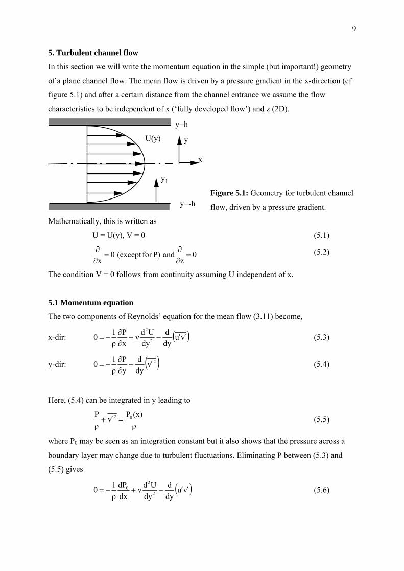
5. Turbulent channel flow

In this section we will write the momentum equation in the simple (but important!) geometry

of a plane channel flow. The mean flow is driven by a pressure gradient in the x-direction (cf

figure 5.1) and after a certain distance from the channel entrance we assume the flow

characteristics to be independent of x (‘fully developed flow’) and z (2D).

U(y)

x

y

y=h

y=-h

y1

Figure 5.1: Geometry for turbulent channel

flow, driven by a pressure gradient.

Mathematically, this is written as

U = U(y), V = 0 (5.1)

0z

andP)for(except0x

=∂∂

=∂∂ (5.2)

The condition V = 0 follows from continuity assuming U independent of x.

5.1 Momentum equation

The two components of Reynolds’ equation for the mean flow (3.11) become,

x-dir: ( vudyd

dyUdν

xP

ρ10 2

2

′′−+∂∂

−= ) (5.3)

y-dir: ( 2vdyd

yP

ρ10 ′−

∂∂

−= ) (5.4)

Here, (5.4) can be integrated in y leading to

ρ(x)Pv

ρP 02 =′+ (5.5)

where P0 may be seen as an integration constant but it also shows that the pressure across a

boundary layer may change due to turbulent fluctuations. Eliminating P between (5.3) and

(5.5) gives

( vudyd

dyUdν

dxdP

ρ10 2

20 ′′−+−= ) (5.6)

10

(5.6) can be integrated in y and choosing the integration interval ∫−

y

h

...dy we obtain

( 0vudydU

dydUνh)(y

dxdP

ρ10

hy

0 −′′−⎟⎟⎠

⎞⎜⎜⎝

⎛−++−=

−=

) , (5.7)

where we have used the fact that the Reynolds stress vanishes on the wall. The evaluation of

the mean shear on the wall may be expressed in terms of the wall shear stress since we have

2w

hyhy

u/ρτdydUμ

ρ1

dydUν ∗

−=−=

≡== (5.8)

Here, we have defined a characteristic velocity, , which is denoted the friction velocity (or

wall velocity). It has a fundamental role when scaling the velocity close to the wall.

∗u

The relation of to other velocities in a flow can be derived using the local friction

coefficient Cf,x

∗u

2/ρU2m

wτ≡ , where Um is a typical (mean) velocity. Substituting for and

knowing that Cf,x is dependent on the Reynolds number, one obtains /Um =

∗u

∗u 2/C x,f. For a

turbulent boundary layer Cf,x = 0.059Rex-1/5 and in a turbulent pipe flow Cf,x = 0.079Re-1/4,

respectively. Thus the ratio /Um will vary weakly with the Reynolds number. ∗u

To see the use of in the scaling of the momentum equation we first eliminate P0 by putting

y = 0 in (5.7), using that U is symmetric and

∗u

vu ′′ = 0 there. This yields

2*

0 uhdxdP

ρ10 −−= (5.9)

Combining with (5.7) gives

vudydUν

hyu0 2

* ′′−+= (5.10)

(5.10) is valid in the whole interval hy ≤ but the different terms balance each other

dependent on where in the interval we are. As the wall proximity is of most interest, it is

useful to introduce the distance from the wall as a new variable, y1 = y + h. In terms of y1,

(5.10) thus becomes

vudydUν

hy1u0

1

12* ′′−+⎟

⎠⎞

⎜⎝⎛ −−= (5.11)

11

(5.11) is of considerable interest since it couples the Reynolds’ stress to the mean flow.

However, the balance between the different terms depend on the y1 position and to elucidate

this it is necessary to scale the equation. This can be done in (at least) two ways, one using h

as the characteristic length, the other /ν, denoted the wall length. The velocity is scaled by

in both cases.

∗u

∗u

Outer scaling: Scaling with h (and ∗u )

(5.11) reduces to

2*1

1

uvu

/h)d(y)d(U/u

huν

hy10

′′−++−= ∗

∗

Introducing the Reynolds no.,νhuRe ∗

∗ = , this expression may also be written as

2*1

1

uvu

/h)d(y)d(U/u

Re1

hy10

′′−++−= ∗

∗

(5.12)

Since in general is a large number, (5.12) is reduced in the center portion of the channel

to

∗eR

2*

1

uvu

hy10

′′−+−= (5.13)

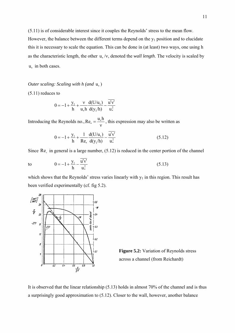
which shows that the Reynolds’ stress varies linearly with y1 in this region. This result has

been verified experimentally (cf. fig 5.2).

Figure 5.2: Variation of Reynolds stress

across a channel (from Reichardt)

It is observed that the linear relationship (5.13) holds in almost 70% of the channel and is thus

a surprisingly good approximation to (5.12). Closer to the wall, however, another balance

12

exists between the terms in (5.12). In particular, the viscous term must be important and it can

be incorporated by another scaling of (5.12).

Inner scaling: Scaling with ν / (and ). ∗u ∗u

The second scaling that may be done is such that the viscous term is weighted by unity. The

proper length scale is then ν/ and (5.11) then becomes ∗u

2*1

1

uvu

)/ud(y)d(U/u

Re1uy10

′′−

ν+⋅

ν+−=

∗

∗

∗

∗ (5.14)

It is customary to introduce the new wall distance

ν

= ∗+

uyy 1 (5.15)

and the new velocity

∗

+ =uUU (5.16)

(5.14) can then be written as

2*uvu

dydU

Rey10

′′−++−=

+

+

∗

+ (5.14)’

With a large value of the Reynolds no., (5.14)’ reduces to

2*uvu

dydU10

′′−+−=

+

+ (5.17)

The distribution of uv close to the wall can been measured in detail with LDV and the results

are shown in figure 5.3. It is observed that the uv-value is almost constant in a large portion of

the wall layer.

Figure 5.3: Distribution of Reynolds

stress close to a wall. (from Karlsson et

al.)

13

5.2 Turbulence production

According to (4.4), the production of turbulent kinetic energy is given by ji,ji Uuu ′′− . For the

channel flow here, this reduces to

dydUvuP ′′−= (5.18)

The minus-sign in (5.18) needs a comment. If we consider the lower half of figure 5.1 and let

a fluid particle move upwards, its v′ component is > 0. But, since the particle starts from a

region with lower mean velocity it will cause a negative u′ where it ends up. Thus, the product

u′v′ is negative and, since dydU > 0, there will be a production of turbulent energy due to this

motion. A similar argument for a particle moving downward also gives a positive production.

We can now use the results of the inner scaling to estimate where the maximum turbulent

production is to be expected. Close to the wall, (5.11) reduces to

⎟⎟⎠

⎞⎜⎜⎝

⎛=′′′−′+−=

1

2* dy

dUUvuUνu0 (5.19)

Multiplying (5.19) by U′ we get

U)Uu(UvuP 2 ′⋅′ν−=′′′−= ∗ (5.20)

Seen as a function of U′, (5.20) can be differentiated to give optimum (maximum) for P. We

have U2uUUuUd

dP 22 ′ν−=′ν−′ν−=′ ∗∗

Thus, at

U′ = (5.21) ν∗ 2/u 2

there is maximum in P which becomes

Pmax = ( )2 (5.22) ν∗ 2/u 2

Since is the wall-value of U′, (5.21) shows that Pmax occurs where this value is halved.

The only thing that must be asserted with this analysis is that the maximum point actually lies

within the wall region so that (5.19) is valid. Before this can be asserted, some knowledge of

the velocity profile is necessary.

ν∗ /u2

14

5.3 Mean velocity profile

The information gained from the two types of scaling leads to a way to estimate the turbuelent

velocity profile. First, (5.17) indicates that close to the wall both the mean velocity and the

Reynolds’ stress are functions of y+, only. Thus,

U+ = f(y+)

and =′′− ∗

2u/vu g(y+) (5.23)

This is denoted a wall-law.

In the outer region, where (5.13) applies, there is no information on U since it is absent in the

equation. However, some information can be obtained from the energy equation for the

fluctuations (4.4). In the outer region, it reduces to

ε+⎟⎠

⎞⎜⎝

⎛ ′+′′ρ

=′′− qvpv1dyd

dydUvu

11

(5.24)

(5.13) shows that vu ′′ is of the order which we can expect also q and p′/ρ to be. Thus we

can write

2u∗

η= ∗

ddF

hu

dydU

1

(5.25)

Integrating this relation from the center of the channel gives

)(Fu

UU 0 η=−

∗

(5.26)

This type of relation is denoted a velocity defect law and is valid in the center portion of the

channel. Closer to the wall, the wall law (5.23) applies and it is natural to ask what happens in

the intermediate region. This can be given some input by considering the velocity derivative

dU/dy1 derived from the two relations (5.23) and (5.26).

Law of the wall (5.23)⇒+

∗+

+

∗ ⋅ν

=⋅⋅=dydfu

dydy

dydfu

dydU 2

11

(5.27)

Law of the wake (5.26) ⇒η

⋅=η

⋅η

⋅= ∗∗ d

dFhu

dyd

ddFu

dydU

11

(5.28)

In the overlap region both relations must hold. Multiplying both sides with gives then∗u/y1

η

η=+

+ ddF

dydfy (5.29)

Here, the left hand side is a function of y+ and the left hand side a function of η. Thus they

must be a constant. This constant is denoted von Karmáns constant (κ) and is roughly 0.41.

Integrating the two relations then give

15

++ κ

= yln1)y(f + constant (5.30)

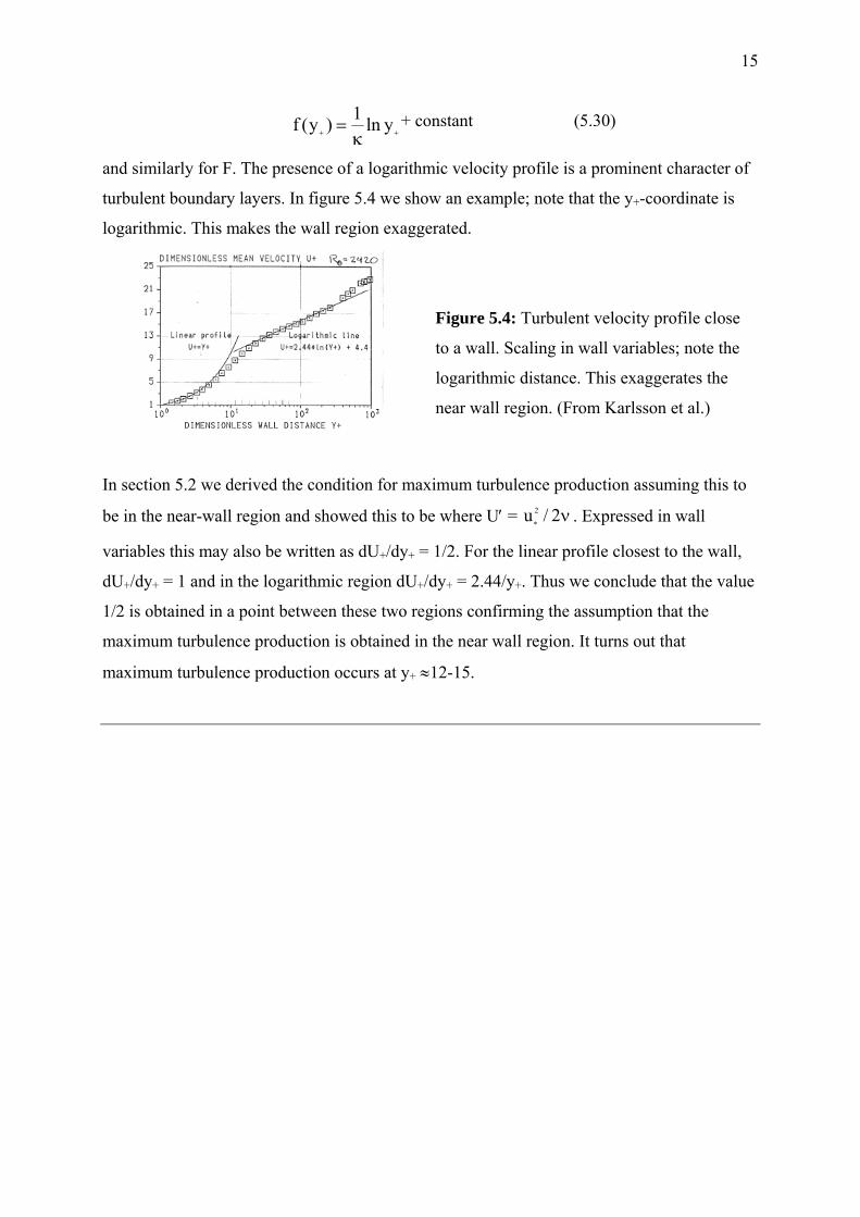
and similarly for F. The presence of a logarithmic velocity profile is a prominent character of

turbulent boundary layers. In figure 5.4 we show an example; note that the y+-coordinate is

logarithmic. This makes the wall region exaggerated.

Figure 5.4: Turbulent velocity profile close

to a wall. Scaling in wall variables; note the

logarithmic distance. This exaggerates the

near wall region. (From Karlsson et al.)

In section 5.2 we derived the condition for maximum turbulence production assuming this to

be in the near-wall region and showed this to be where U′ = ν∗ 2/u 2 . Expressed in wall

variables this may also be written as dU+/dy+ = 1/2. For the linear profile closest to the wall,

dU+/dy+ = 1 and in the logarithmic region dU+/dy+ = 2.44/y+. Thus we conclude that the value

1/2 is obtained in a point between these two regions confirming the assumption that the

maximum turbulence production is obtained in the near wall region. It turns out that

maximum turbulence production occurs at y+ ≈12-15.

16

6. Kolmogorov microscales

Turbulence is generated at fairly large scales but due to non-linear interactions smaller and

smaller scales are involved. At the smallest level, the energy is lost to viscous dissipation and

it was originally suggested that this process was isotropic, i.e. does not have a preferred

orientation. At this level, the scales should be governed by viscosity (ν) and the dissipation

rate (ε) only. These quantities have dimensions m2/s and m2/s3, respectively, so the design of

length, time and velocity scales based on these quantities is straight forward and yield the

following set:

Length scale: ( ) 4/13 / εν=η

Time scale: (6.1a-c) ( ) 2/1/ εν=τ

Velocity scale: ( ) 4/1νε=ϑ

These are called the Kolmogorov microscales. The length scale is the smallest scale in a

turbulent flow.

A couple of points related to these scales are of interest.

• The Reynolds number based on the microscales is equal to unity.

• For turbulence in balance, the dissipation rate must be equal to the energy transfer

from the largest scales, where energy is put in. By knowing the energy input in e.g. a

stirring process it is thus possible to determine the microscales.

17

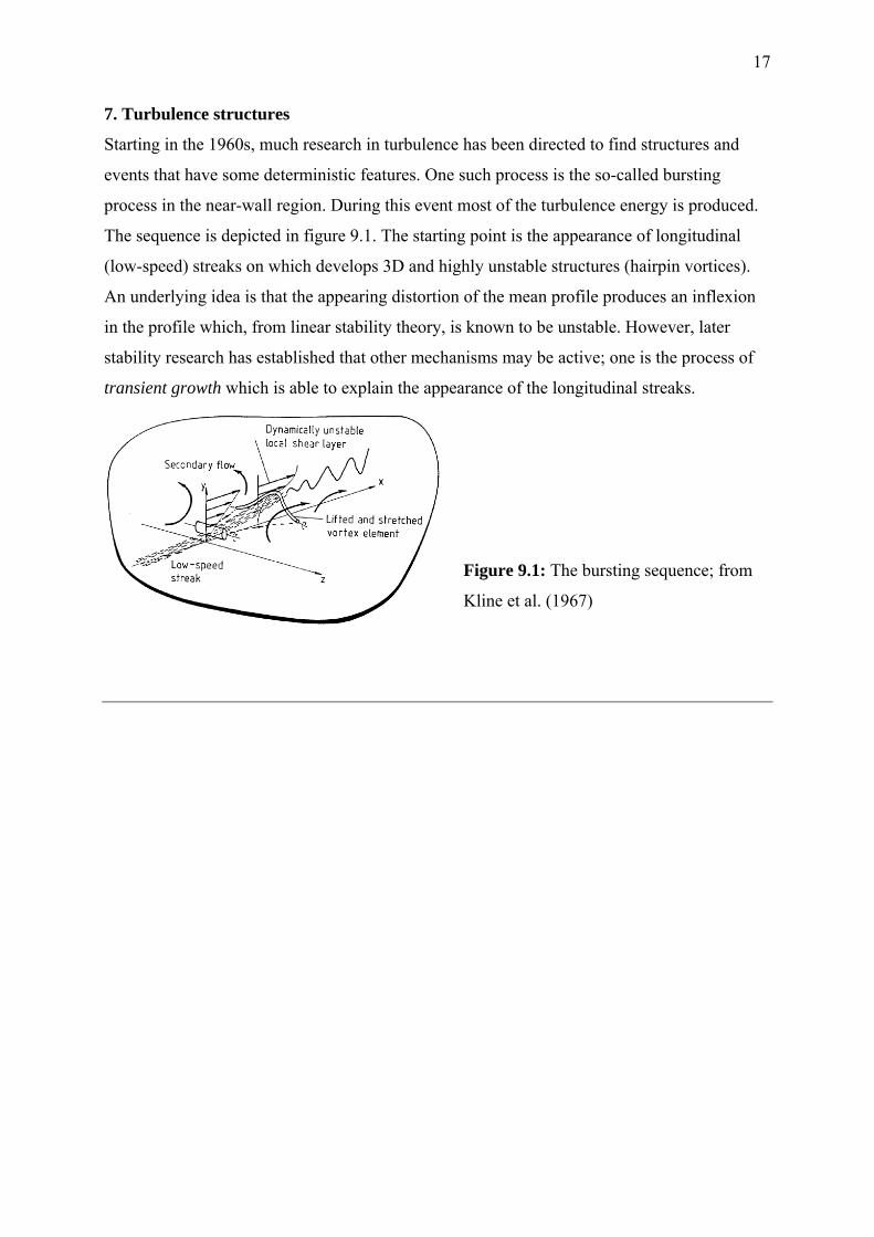
7. Turbulence structures

Starting in the 1960s, much research in turbulence has been directed to find structures and

events that have some deterministic features. One such process is the so-called bursting

process in the near-wall region. During this event most of the turbulence energy is produced.

The sequence is depicted in figure 9.1. The starting point is the appearance of longitudinal

(low-speed) streaks on which develops 3D and highly unstable structures (hairpin vortices).

An underlying idea is that the appearing distortion of the mean profile produces an inflexion

in the profile which, from linear stability theory, is known to be unstable. However, later

stability research has established that other mechanisms may be active; one is the process of

transient growth which is able to explain the appearance of the longitudinal streaks.

Figure 9.1: The bursting sequence; from

Kline et al. (1967)

18

References

There is a multitude of books on turbulence of which the list below is just a short example.

Despite its age, the book by Tennekes and Lumley is still a quite useful opener to the subject

and may be recommended. A more modern book, where turbulence modelling and

simulations are treated, is the book by Pope.

Bradshaw P. 1985, An Introduction to Turbulence and its Measurement, Pergamon Press

Durbin P. and Pettersson Reif B.A. 2001, Statistical Theory and modelling for Turbulent Flows, Wiley.

Landahl M.T. and Mollo-Christensen E. 1986, Turbulence and random processes in fluid mechanics,

Cambridge University Press.

Lesieur M. 1990, Turbulence in Fluids, Kluwer.

McComb W.D. 1990, The Physics of Fluid Turbulence, Oxford Science Publications.

Pope S.B. 2000, Turbulent Flows, Cambridge University Press

Rotta J.C. 1972, Turbulente Strömungen, B.G. Teubner, Stuttgart

Schlichting H. 1979, Boundary layer theory, 7th edition, McGraw Hill

Tennekes H. and Lumley J.L. 1972, A first course in turbulence, MIT Press.

Townsend A.A. 1980, The structure of turbulent shear flow, 2nd edition, Cambridge University Press.

Wilcox D.C. 1993, Turbulence Modeling for CFD, DCW Industries.