Introduction to the Transportation Network Design ir... · · 2015-11-23Introduction to the...

Introduction to the Transportation Network Design

Assoc. Prof. Dr. Huseyin Ceylan Pamukkale University

Department of Civil Engineering Denizli, Turkey

Contents

• Motivation

• Network terminology

• Introduction

• Objective

• Traffic assignment – All-or-Nothing assignment,

– Incremental assignment,

– User-Equilibrium (UE) assignment,

– System Optimum (SO) assignment,

– Stochastic User-Equilibrium (SUE) assignment,

• Solution to the NDP

Transportation network design

Motivation


Social and economical development

Importance of networks

(water supply, energy supply, communication, transportation)

Motivation


Increasing socio-

economical needs

Varied activities

Mobility demand

Private car ownership and usage

Motivation


Contents

• Motivation


• Introduction

• Objective








Network Terminology

• A transport network may be formally represented as a set of links and a set of nodes.

• A link connects two nodes and a node connects two or more links.

• Links may be either directed or undirected.


Network Terminology

• A movement in a transportation network corresponds to a flow with a distinct Origin (O) and Destination (D).

• O-Ds may correspond to specific buildings like a house or and office, or to zones (districts).

• O-Ds are represented by a kind of node, referred to as a centroid.

• Each centroid is connected to one or more nodes by a kind of link referred to as a connector.


Network Terminology

• Links may have various characteristics.

• In the context of transportation network analysis, the following are some of the characteristics of interest:

– Link length (in meters or perhaps in average vehicles)

– Link cost (generally travel time) and

– Link capacity (maximum flow)


Contents

• Motivation


• Introduction

• Objective








Introduction

• Transportation Network Design Problem (NDP) concerns the configuration of a network to achieve specified objectives.


NDP


NDP


1 2 3 4

1 0 741 710 200

2 565 0 688 508

3 604 490 0 322

4 577 888 456 0

NDP


NDP


Lane addition

NDP


Building reversible lanes

NDP


Congestion pricing

NDP


Widening traffic lanes

NDP


Road resurfacing

NDP


Signal controlled intersections

NDP


Intelligent transportation systems

Introduction

• There are two forms of the problem

– The continuous network design problem

– The discrete network design problem


Introduction

• The continuous network design problem takes the network topology as given and is concerned with the parameterization of the network. For example:

– The determination of road width (number of lanes);

– The calculation of traffic signal timings;

– The setting of user charges (public transport fares, road tolls, etc)


Introduction

• The discrete network design problem is concerned with the topology of the network. For example:

– A road closure scheme;

– The provision of a new public transport service (represented as a new set of links); and

– The construction of a new road rail link, perhaps a bridge, a tunnel or a bypass.


Introduction

User benefits

Construction of an extra lane

(increases the capacity of the road)

Allocation of more capacity to one signal-controlled link by

increasing green time per cycle

Imposition or increasing user charges

(can bring about benefits to society as a whole through greater

economic efficiency)


Cost of network alteration

Construction of an extra lane

(brings cost)

Reduces the capacity of some other link(s) through reduced green

time per cycle

Imposition or increasing user

charges (may result in extra costs for certain

users)

TRADE-OFF

Contents

• Motivation


• Introduction

• Objective








Objective

• Traditional network design has been concerned with the minimization of system cost (equal to the sum of link flows times link costs).

ci : the cost (travel time) on link i

vi : the flow on link i (TRAFFIC ASSIGNMENT)

si : the value of the design parameter for link i


,i i i ii I

SC v c v s

Contents

• Motivation


• Introduction

• Objective








Traffic Assignment

• The process of allocating given set of trip interchanges to the specified transportation system is usually referred to as traffic assignment.

• The fundamental aim of the traffic assignment process is to reproduce on the transportation system, the pattern of vehicular movements which would be observed when the travel demand represented by the trip matrix, or matrices, to be assigned is satisfied.


Traffic Assignment


Traffic Assignment

• The major aims of traffic assignment procedures are: – To estimate the volume of traffic on the links of the network,

– To obtain aggregate network measures, e.g. total vehicular flows, total distance covered by the vehicle, total system travel time.

– To estimate zone-to-zone travel costs(times) for a given level of demand.

– To obtain reasonable link flows and to identify heavily congested links.

– To estimate the routes used between each origin to destination(O-D) pair.

– To obtain turning movements for the design of future junctions.


Traffic Assignment

• The types of traffic assignment models: – All-or-Nothing assignment,






Contents

• Motivation


• Introduction

• Objective








All-or-Nothing Assignment

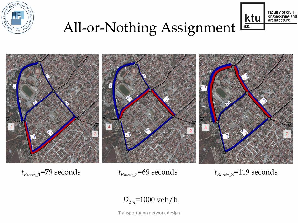
• The trips from any origin zone to any destination zone are loaded onto a single, minimum cost, path between them.


Path no Route Free flow travel time

1 1-3-4 6 mins

2 1-2-4 8 mins

3 1-2-3-4 10 mins

4 1-3-2-4 12 mins

1 4 2000 veh/hq

_ 1 2000 veh/hPathf



tRoute_1=79 seconds tRoute_2=69 seconds tRoute_3=119 seconds

D2-4=1000 veh/h




vRoute_2=1000 veh/h vRoute_1=0 vRoute_3=0


• This model in unrealistic as:

– Only one path between every Origin-Destination (O-D) pair is

utilized even if there is another path with the same or nearly same travel cost.

– Traffic on links is assigned without consideration of whether or

not there is adequate capacity or heavy congestion



• This model may be used:

– For uncongested networks where there are a few alternative

routes and they have a large difference in travel cost (travel time)

– To identify the desired path which the drivers would like to

travel in the absence of congestion


Incremental Assignment

• This is a process in which fractions of traffic volumes are assigned in steps.

• In each step, a fixed proportion of total demand is assigned, based on all-or-nothing assignment.

• After each step, link travel times are recalculated based on link volumes.





D2-4=1000 veh/h




vRoute_2=500 veh/h vRoute_1=500 veh/h vRoute_3=0

Contents

• Motivation


• Introduction

• Objective








Wardrop’s Principles

• John Glen Wardrop (1920 - 1989) was an English transport analyst who developed Wardrop's first and second principles of equilibrium.

• The concepts are related to the idea of Nash equilibrium in game theory developed separately. However, in transportation networks, there are many players, making the analysis complex.



• Wardrop's first principle of route choice became accepted as a sound and simple behavioral principle to describe the spreading of trips over alternate routes due to congested conditions.

• Wardrop's first principle states: The journey times in all routes actually used are equal and less than those which would be experienced by a single vehicle on any unused route.


1 2 D12 = 50

v1= 1, t1 = 10

v2= 1, t2 = 12

v3= 1, t3 = 24 TTT=1x10+1x12+1x24=46


• Wardrop's first principle of route choice became accepted as a sound and simple behavioral principle to describe the spreading of trips over alternate routes due to congested conditions.

• Wardrop's first principle states: The journey times in all routes actually used are equal and less than those which would be experienced by a single vehicle on any unused route.


1 2 D12 = 50

v1= 21, t1 = 21

v2= 29, t2 = 21

v3= 0, t30 = 24 TTT=21x21+29x21+0x24=1050


• Each user non-cooperatively seeks to minimize his cost of transportation. The traffic flows that satisfy this principle are usually referred to as "user equilibrium" (UE) flows, since each user chooses the route that is the best.

• Specifically, a user-optimized equilibrium is reached when no user may lower his transportation cost through unilateral action.


1 2 D12 = 50

v1= 21, t1 = 21

v2= 29, t2 = 21

v3= 0, t30 = 24 TTT=21x21+29x21+0x24=1050


• Wardrop's second principle states: At equilibrium the average journey time is minimum.

• This implies that each user behaves cooperatively in choosing his own route to ensure the most efficient use of the whole system.

• Traffic flows satisfying Wardrop's second principle are generally deemed "system optimal" (SO).


1 2 D12 = 50

v1= 18, t1 = 23

v2= 32, t2 = 19

v3= 0, t3 = 24 TTT=18x23+32x19+0x24=1022

User-Equilibrium (UE)

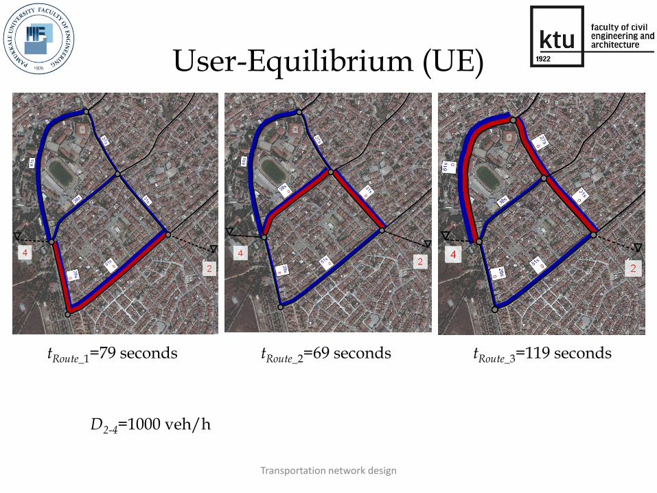
• The user equilibrium assignment is based on Wardrop's first principle, which states that no driver can unilaterally reduce his/her travel costs by shifting to another route.

• For each O-D pair, at user equilibrium, the travel time on all used paths is equal, and (also) less than or equal to the travel time that would be experienced by a single vehicle on any unused path.

• If it is assumed that drivers have perfect knowledge about travel costs on a network and choose the best route according to Wardrop's first principle, this behavioral assumption leads to deterministic user equilibrium.


(1)

(2)

min ( )

a

a A

z t x dxav

0

, ,rs

k rs rs

k K

f D r R s S k K

, , , ,rs

rs rs

a k a k rs

rs k K

v f r R s S a A k K

0 , ,rs

k rsf r R s S k K

(3)

(4)

s.t.

• This problem is equivalent to the following nonlinear mathematical optimization program,



k is the path, va equilibrium flows on link a, ta travel time on link a, fkrs flow

on path k connecting O-D pair r-s, Drs trip rate between r and s.




D2-4=1000 veh/h

System Optimum (SO)

• The system optimum assignment is based on Wardrop's second principle, which states that drivers cooperate with one another in order to minimize total system travel time.

• This assignment can be thought of as a model in which congestion is minimized when drivers are told which routes to use.

• Obviously, this is not a behaviorally realistic model, but it can be useful to transport planners and engineers, trying to manage the traffic to minimize travel costs and therefore achieve an optimum social equilibrium.


(5)

(6)

min ( ) a a a

a

z v t v

, ,rs

k rs rs

k K

f D r R s S k K

, , , ,rs

rs rs

a k a k rs

rs k K

v f r R s S a A k K

0 , ,rs

k rsf r R s S k K

(7)

(8)

s.t.

• This problem is equivalent to the following nonlinear mathematical optimization program,

System Optimum (SO)


k is the path, va equilibrium flows on link a, ta travel time on link a, fkrs flow

on path k connecting O-D pair r-s, Drs trip rate between r and s.

System Optimum (SO)



D2-4=1000 veh/h

System Optimum (SO)




Assignment TTT

AoN 136000

UE 92000

SO 85354

Example - I

• Demonstration of the common assignment methods.

• This network has two nodes having two path as links with constant travel time.

• Total flows from 1 to 2, D12 = 12 vehicles


1 2

v1

v2

t1=10

t2=15

Figure 1: Two Link Problem with constant travel time function

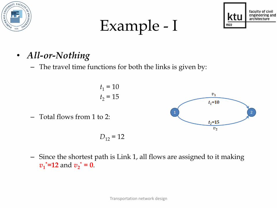
Example - I

• All-or-Nothing – The travel time functions for both the links is given by:

t1 = 10

t2 = 15

– Total flows from 1 to 2:

D12 = 12

– Since the shortest path is Link 1, all flows are assigned to it making v1

*=12 and v2* = 0.


Example - I

• User Equilibrium – Substituting the travel time in Equations 1-4 yield to:

– Substituting v2 =12 – v1, in the above formulation will yield the unconstrained formulation as below:

– Differentiate the above equation with respect to v1 and equate to zero, and solving for v1 and then v2 leads to the solution v1

*=12 and v2* = 0


1 2

1 2

1 2

1 2

min ( ) 10 15

10 15

subject to: 12

a

a A

z t x dx dv dv

v v

v v

av v v

0 0 0

1 1min 10 15 12 z v v

Example - I

• System Optimum – Substituting the travel time in Equations 5-8, we get the following:

– Substituting v2 = 12 – v1, the above formulations take the following form:


*=12, v2* = 0 and z(v*)=120.


1 2

1 2

min 10 15

10 15

z v v

v v

1 1min 10 15 12 z v v

Comparison of results

• After solving each of the formulations the results are given in the following table.


Type t1 t2 v1 v2 Z(x*) TTT

AON 10 15 12 0 120 120

UE 10 15 12 0 120 120

SO 10 15 12 0 120 120

Example - II

• This network has two nodes having two path as links with travel times as functions of the link flow.

• Total flows from 1 to 2, D12 = 12 vehicles


1 2

v1

v2

t1=10+3v1

t2=15+2v2

Figure 1: Two Link Problem with constant travel time function

Example - II

• All-or-Nothing – Assume that v1, v2 = 0 which makes t1 = 10 and t2 = 15.

– Since the shortest path is Link 1, all flows are assigned to it making v1

*=12 and v2* = 0.


Example - II • User Equilibrium

– Substituting the travel time in Equations 1-4 yield to:

– Substituting v2 =12 – v1, in the above formulation will yield the unconstrained formulation as below:


*=5.8 and v2* = 6.2


1 2

1 1 2 2

2 21 2

1 2

1 2

min ( ) 10 3 15 2

3 2 10 15

2 2subject to: 12

aa

z t x dx v dv v dv

v vv v

v v

A

av v v

0 0 0

2211

1 1

2 123min 10 15 12

2 2

vvz v v

Example - II

• System Optimum – Substituting the travel time in Equations 5-8, we get the following:

– Substituting v2 = 12 – v1, the above formulations take the following form:


*=5.3, v2* =6.7 and z(v*)=327.55


1 1 2 2

2 2

1 1 2 2

min 10 3 15 2

10 3 15 2

z v v v v

v v v v

22

1 1 1 1min 10 3 15 12 2 12 z v v v v

Comparison of results

• After solving each of the formulations the results are given in the following table.


Type t1 t2 v1 v2 Z(x*) TTT

AON 10 15 12 0 467.4 552

UE 27.4 27.4 5.8 6.2 239.0 329

SO 30.1 25.6 5.3 6.7 327.5 328

Contents

• Motivation


• Introduction

• Objective








Stochastic User Equilibrium • A variant on Wardrop’s first principle (UE) is the stochastic user equilibrium (SUE),

wherein no driver can unilaterally change routes to improve his/her perceived travel times.

• In the SUE, the assumption that travelers have perfect information on the road network is relaxed.

• Travelers experience perception error. The SUE behavioral assumption brings some advantages over DUE in that it represents behavior more realistically


1 2 D12 = 50

v1= 20, t1 = 21

v2= 27, t2 = 20

v3= 3, t30 = 24

Contents

• Motivation


• Introduction

• Objective








Solution to the NDP

• In a road network to be optimized, there is an interaction between the design parameters and the routes chosen by individual road users.

• The problem falls within the framework of a leader-follower (or Stackelberg) game, where the designer (i.e. transport planner) is the leader and the user is the follower (Fisk, 1984).

• When drivers follow Wardrop's (1952) first principle, (i.e UE), the problem is called the “equilibrium network design problem (ENDP), which is normally non-convex.


Solution to the NDP

• In the literature, this leader-follower game has widely been formulated as a combined bi-level problem.

• The bi-level programming (BLP) problem is a special case of multilevel programming problems with a two level structure.

• The problem can be expressed as follows: the transport planner, wishes to optimize the control variables in the upper level, and the users response to these controls in UE manner in the lower level.


Solution to the NDP

• In the last decades, several solution methods have been developed to solve bi-level ENDP.

• These methods can be classified as deterministic and stochastic in nature.

• The deterministic methods can be classified as the linearization, sensitivity analysis and gradient based local search approaches that require substantial gradient information to find a solution.

• Stochastic methods, in particular genetic algorithms, differential evolution, harmony search, ant colony optimization, etc., have widely been employed to the solution of the ENDP.


Modified differential evolution algorithm for the continuous

network design problem

Assoc. Prof. Dr. Ozgur BASKAN Assoc. Prof. Dr. Huseyin CEYLAN

Department of Civil Engineering

Engineering Faculty Pamukkale University

Denizli / Turkey


Content

Objectives and problem definition

Background

Differential evolution algorithm

Numerical application

Results

Findings and future studies


Objectives

This study aims

• To develop a new solution method, which is capable to find near optimal solutions of the CNDP within less computational time

• To improve the base DE algorithm in order to

facilitate the solution process.


Problem definition

CNDP is

• To determine the set of link capacity expansions

• To find corresponding equilibrium link flows

and …

Considering both objectives,

“The measure of performance index for the network should be optimal”


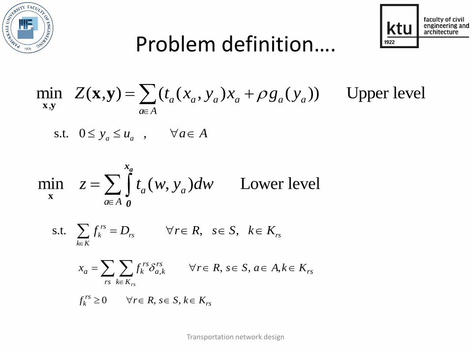
Problem definition….

min ( ) ( ( , ) ( )) Upper levela a a a a a,

a A

Z , t x y x g y

x y

x y

s.t. 0 ,a ay u a A

min ( , ) Lower levela a

a A

z t w y dw

x

ax

0

s.t. , ,rs

k rs rs

k K

f D r R s S k K

rs Kk

rsrs

kars

ka

rs

KkAaSsRrfx ,,,,

rsrs

k KkSsRrf ,,0


Background Reference Objective Decision Lower level Method Steenbrick (1974)

Travel and Construction cost

Capacity expansion

SO

Iterative Optimization Algorithm (IOA)

Abdulaal and Leblanc (1979)

DUE

Powell’s and Hooke-Jeeves (HJ) methods

Marcotte (1983) Exact algorithm Marcotte (1986) Four heuristics based on

IOA Friesz et al. (1992) SA and projection

methods Davis (1994)

SUE Generalized reduced gradient method, sequential quadratic programming

Meng et al. (2001)

DUE

Augmented lagrangian method

Chiou (2005) Four gradient based methods

Gao et al. (2007) Total travel time/cost Gradient based method

Xu et al. (2009) Travel and Construction cost

SA and Genetic Algorithm (GA)

Mathew and Sarma (2009) Total travel time/cost GA

Wang and Lo (2010)

Travel and Construction cost

Mixed integer linear program

Baskan (2012) Harmony Search (HS)

Baskan (2013) Cuckoo Search (CS)


Differential Evolution Algorithm

• DE is a simple and powerful algorithm which is introduced by Storn and Price (1995).

• Three control parameters are used to control optimization process.

– Number of populations (NP)

– Mutation factor (F)

– Crossover rate (CR)


Differential Evolution Algorithm…

The steps of the DE algorithm

• Generation of the initial population

• Mutation

• Crossover

• Selection



Improvement mechanisms First improvement on the standard DE is to take different mutation strategies into account.

Aim of this improvement

“To take the effect of best solution vector determined at previous generation into account”

1, 2, 3,,

1, , 1 2,otherwise

( ), if rand (0,1) MSCR

( ),

t t ti i ij t

i t best t ti i i

y F y ym

y F y y



The second improvement mechanism is a kind of embedding a local search mechanism to the DE algorithm.

Aim of this improvement

“To push the best solution existed in the population towards to

the global or near global optimum one step closer”


Numerical application

1

4

3

2

5

16

11

6 13

15

2

1

3

1

6

7 4

5

18

17 10

12

8

14

Scenario D16 D61 Total demand 1 5 10 15 2 15 25 40

9


Numerical application…

4)(),(aa

aaaaaa

y

xyxt

The travel time function is:

The upper level objective function is defined as:

Aa

aaaaaa,

ydxyxt,Z )),(()(min yxyx

s.t. 0 ,a ay u a A


Results Scenario 1 Scenario 2

MODE DE SA GA MODE DE SA GA

y1 0 0 0 0 0 0 0 0

y2 0 0 0.47 0 10.13 9.29 9.12 11.98

y3 0 0 0.65 0 17.54 17.34 18.12 16.24

y4 0 0 0 0 0 0 0 0

y5 0 0 0 0 0 0 0 0

y6 5.24 4.93 6.53 4.47 5.95 6.12 4.98 5.40

y7 0 0 0.80 0 0 0 0.11 0

y8 0 0 0.25 0 3.48 2.69 1.58 6.04

y9 0 0 0 0 0 0.12 0 0

y10 0 0 0 0 0.01 0.04 0 0

y11 0 0 0 0 0 0 0 0

y12 0 0 0 0 0 0 0 0

y13 0 0 0 0 0 0 0 0

y14 0 0 0.84 0 12.66 12.25 11.66 12.28

y15 0 0 0.14 0 0 0 2.97 0.82

y16 7.61 7.69 7.34 7.54 19.99 19.94 19.71 19.99

y17 0 0 0 0 0 0.12 0 0

y18 0 0 0 0 0 0 0 0

Z 190.33 190.43 205.89 191.26 729.58 730.43 739.54 744.39

NUE 396 860 15000 50000 759 1090 22500 50000


Results…

0 10 20 30 40 50 60 70 80 90150

200

250

300

350

400

450

500

550

600

650

700

Number of generations

Obj

ecti

ve

func

tion

val

ue

DE

MODE

190.43190.33

Convergence graph for Scenario 1


Results… Convergence graph for Scenario2

0 20 40 60 80 100 120700

750

800

850

900

950

1000

1050

1100

1150

1200

Number of generations

Obj

ecti

ve

func

tion

val

ue

MODE

DE

729.58 730.43


Findings and future studies

• The improved version of the base DE achieved better solutions in all scenarios in terms of objective function value and number of UE assignments in comparison with the DE, SA and GA.

• The developed mutation strategy and local search operator have facilitated the rate of convergence of the base DE algorithm.


Findings and future studies…

“It is necessary to test the developed algorithm for large-scale road network applications”


Thank you for your attention


Introduction to the Transportation Network Design ir... · · 2015-11-23Introduction to the...

Documents

Transcript of Introduction to the Transportation Network Design ir... · · 2015-11-23Introduction to the...