Introduction to Tensor Calculus Continuum Mechanics - J. Heinbockel
373
Introduction to Tensor Calculus and Continuum Mechanics by J.H. Heinbockel Department of Mathematics and Statistics Old Dominion University
-
Upload
harikumar-andem -
Category
Documents
-
view
220 -
download
0
Transcript of Introduction to Tensor Calculus Continuum Mechanics - J. Heinbockel

8/6/2019 Introduction to Tensor Calculus Continuum Mechanics - J. Heinbockel
http://slidepdf.com/reader/full/introduction-to-tensor-calculus-continuum-mechanics-j-heinbockel 1/372
Introduction toTensor Calculus
andContinuum Mechanics
by J.H. Heinbockel
Department of Mathematics and Statistics
Old Dominion University
8/6/2019 Introduction to Tensor Calculus Continuum Mechanics - J. Heinbockel
http://slidepdf.com/reader/full/introduction-to-tensor-calculus-continuum-mechanics-j-heinbockel 2/372
PREFACE
This is an introductory text which presents fundamental concepts from the subject
areas of tensor calculus, differential geometry and continuum mechanics. The material
presented is suitable for a two semester course in applied mathematics and is flexible
enough to be presented to either upper level undergraduate or beginning graduate students
majoring in applied mathematics, engineering or physics. The presentation assumes the
students have some knowledge from the areas of matrix theory, linear algebra and advanced
calculus. Each section includes many illustrative worked examples. At the end of each
section there is a large collection of exercises which range in difficulty. Many new ideas
are presented in the exercises and so the students should be encouraged to read all the
exercises.
The purpose of preparing these notes is to condense into an introductory text the basic
definitions and techniques arising in tensor calculus, differential geometry and continuummechanics. In particular, the material is presented to (i) develop a physical understanding
of the mathematical concepts associated with tensor calculus and (ii) develop the basic
equations of tensor calculus, differential geometry and continuum mechanics which arise
in engineering applications. From these basic equations one can go on to develop more
sophisticated models of applied mathematics. The material is presented in an informal
manner and uses mathematics which minimizes excessive formalism.
The material has been divided into two parts. The first part deals with an introduc-
tion to tensor calculus and differential geometry which covers such things as the indicial
notation, tensor algebra, covariant differentiation, dual tensors, bilinear and multilinear
forms, special tensors, the Riemann Christoffel tensor, space curves, surface curves, cur-
vature and fundamental quadratic forms. The second part emphasizes the application of
tensor algebra and calculus to a wide variety of applied areas from engineering and physics.
The selected applications are from the areas of dynamics, elasticity, fluids and electromag-
netic theory. The continuum mechanics portion focuses on an introduction of the basic
concepts from linear elasticity and fluids. The Appendix A contains units of measurements
from the Systeme International d’Unites along with some selected physical constants. The
Appendix B contains a listing of Christoffel symbols of the second kind associated withvarious coordinate systems. The Appendix C is a summary of useful vector identities.
J.H. Heinbockel, 1996

8/6/2019 Introduction to Tensor Calculus Continuum Mechanics - J. Heinbockel
http://slidepdf.com/reader/full/introduction-to-tensor-calculus-continuum-mechanics-j-heinbockel 3/372
8/6/2019 Introduction to Tensor Calculus Continuum Mechanics - J. Heinbockel
http://slidepdf.com/reader/full/introduction-to-tensor-calculus-continuum-mechanics-j-heinbockel 4/372
INTRODUCTION TOTENSOR CALCULUS
ANDCONTINUUM MECHANICS
PART 1: INTRODUCTION TO TENSOR CALCULUS
§1.1 INDEX NOTATION . . . . . . . . . . . . . . . . . . 1
Exercise 1.1 . . . . . . . . . . . . . . . . . . . . . . . . . . 28
§1.2 TENSOR CONCEPTS AND TRANSFORMATIONS . . . . 35
Exercise 1.2 . . . . . . . . . . . . . . . . . . . . . . . . . . . 54
§1.3 SPECIAL TENSORS . . . . . . . . . . . . . . . . . . 65
Exercise 1.3 . . . . . . . . . . . . . . . . . . . . . . . . . . . 101
§1.4 DERIVATIVE OF A TENSOR . . . . . . . . . . . . . . 108
Exercise 1.4. . . . . . . . . . . . . . . . . . . . . . . . . . .
123§1.5 DIFFERENTIAL GEOMETRY AND RELATIVITY . . . . 129
Exercise 1.5 . . . . . . . . . . . . . . . . . . . . . . . . . . . 162
PART 2: INTRODUCTION TO CONTINUUM MECHANICS
§2.1 TENSOR NOTATION FOR VECTOR QUANTITIES . . . . 171
Exercise 2.1 . . . . . . . . . . . . . . . . . . . . . . . . . . . 182
§2.2 DYNAMICS . . . . . . . . . . . . . . . . . . . . . . 187
Exercise 2.2 . . . . . . . . . . . . . . . . . . . . . . . . . . . 206
§2.3 BASIC EQUATIONS OF CONTINUUM MECHANICS . . . 211
Exercise 2.3 . . . . . . . . . . . . . . . . . . . . . . . . . . . 238
§2.4 CONTINUUM MECHANICS (SOLIDS) . . . . . . . . . 243
Exercise 2.4 . . . . . . . . . . . . . . . . . . . . . . . . . . . 272
§2.5 CONTINUUM MECHANICS (FLUIDS) . . . . . . . . . 282
Exercise 2.5 . . . . . . . . . . . . . . . . . . . . . . . . . . . 317
§2.6 ELECTRIC AND MAGNETIC FIELDS . . . . . . . . . . 325
Exercise 2.6 . . . . . . . . . . . . . . . . . . . . . . . . . . . 347
BIBLIOGRAPHY . . . . . . . . . . . . . . . . . . . . . 352
APPENDIX A UNITS OF MEASUREMENT . . . . . . . 353
APPENDIX B CHRISTOFFEL SYMBOLS OF SECOND KIND 355
APPENDIX C VECTOR IDENTITIES . . . . . . . . . . 362
INDEX . . . . . . . . . . . . . . . . . . . . . . . . . . 363

8/6/2019 Introduction to Tensor Calculus Continuum Mechanics - J. Heinbockel
http://slidepdf.com/reader/full/introduction-to-tensor-calculus-continuum-mechanics-j-heinbockel 5/372
1
PART 1: INTRODUCTION TO TENSOR CALCULUS
A scalar field describes a one-to-one correspondence between a single scalar number and a point. An n-
dimensional vector field is described by a one-to-one correspondence between n-numbers and a point. Let us
generalize these concepts by assigning n-squared numbers to a single point or n-cubed numbers to a single
point. When these numbers obey certain transformation laws they become examples of tensor fields. In
general, scalar fields are referred to as tensor fields of rank or order zero whereas vector fields are called
tensor fields of rank or order one.
Closely associated with tensor calculus is the indicial or index notation. In section 1 the indicial
notation is defined and illustrated. We also define and investigate scalar, vector and tensor fields when they
are subjected to various coordinate transformations. It turns out that tensors have certain properties which
are independent of the coordinate system used to describe the tensor. Because of these useful properties,
we can use tensors to represent various fundamental laws occurring in physics, engineering, science and
mathematics. These representations are extremely useful as they are independent of the coordinate systems
considered.
§1.1 INDEX NOTATION
Two vectors A and B can be expressed in the component form
A = A1 e1 + A2 e2 + A3 e3 and B = B1 e1 + B2 e2 + B3 e3,
where e1, e2 and e3 are orthogonal unit basis vectors. Often when no confusion arises, the vectors A and
B are expressed for brevity sake as number triples. For example, we can write
A = (A1, A2, A3) and B = (B1, B2, B3)
where it is understood that only the components of the vectors A and B are given. The unit vectors would
be represented
e1 = (1, 0, 0), e2 = (0, 1, 0), e3 = (0, 0, 1).
A still shorter notation, depicting the vectors A and B is the index or indicial notation. In the index notation,
the quantities
Ai, i = 1, 2, 3 and B p, p = 1, 2, 3
represent the components of the vectors A and B. This notation focuses attention only on the components of
the vectors and employs a dummy subscript whose range over the integers is specified. The symbol Ai
refers
to all of the components of the vector A simultaneously. The dummy subscript i can have any of the integer
values 1, 2 or 3. For i = 1 we focus attention on the A1 component of the vector A. Setting i = 2 focuses
attention on the second component A2 of the vector A and similarly when i = 3 we can focus attention on
the third component of A. The subscript i is a dummy subscript and may be replaced by another letter, say
p, so long as one specifies the integer values that this dummy subscript can have.

8/6/2019 Introduction to Tensor Calculus Continuum Mechanics - J. Heinbockel
http://slidepdf.com/reader/full/introduction-to-tensor-calculus-continuum-mechanics-j-heinbockel 6/372
2
It is also convenient at this time to mention that higher dimensional vectors may be defined as ordered
n−tuples. For example, the vector
X = (X 1, X 2, . . . , X N )
with components X i, i = 1, 2, . . . , N is called a N −dimensional vector. Another notation used to represent
this vector is X = X 1 e1 + X 2 e2 + · · · + X N eN
where
e1, e2, . . . , eN are linearly independent unit base vectors. Note that many of the operations that occur in the use of the
index notation apply not only for three dimensional vectors, but also for N −dimensional vectors.
In future sections it is necessary to define quantities which can be represented by a letter with subscripts
or superscripts attached. Such quantities are referred to as systems. When these quantities obey certain
transformation laws they are referred to as tensor systems. For example, quantities like
Akij eijk δij δji Ai Bj aij.
The subscripts or superscripts are referred to as indices or suffixes. When such quantities arise, the indices
must conform to the following rules:
1. They are lower case Latin or Greek letters.
2. The letters at the end of the alphabet (u, v, w, x, y, z) are never employed as indices.
The number of subscripts and superscripts determines the order of the system. A system with one index
is a first order system. A system with two indices is called a second order system. In general, a system with
N indices is called a N th order system. A system with no indices is called a scalar or zeroth order system.
The type of system depends upon the number of subscripts or superscripts occurring in an expression.
For example, Aijk and Bm
st , (all indices range 1 to N), are of the same type because they have the same
number of subscripts and superscripts. In contrast, the systems Aijk and C mn
p are not of the same type
because one system has two superscripts and the other system has only one superscript. For certain systems
the number of subscripts and superscripts is important. In other systems it is not of importance. The
meaning and importance attached to sub- and superscripts will be addressed later in this section.
In the use of superscripts one must not confuse “powers ”of a quantity with the superscripts. For
example, if we replace the independent variables (x, y, z) by the symbols (x1, x2, x3), then we are letting
y = x2 where x2 is a variable and not x raised to a power. Similarly, the substitution z = x3 is the
replacement of z by the variable x3
and this should not be confused with x raised to a power. In order towrite a superscript quantity to a power, use parentheses. For example, (x2)3 is the variable x2 cubed. One
of the reasons for introducing the superscript variables is that many equations of mathematics and physics
can be made to take on a concise and compact form.
There is a range convention associated with the indices. This convention states that whenever there
is an expression where the indices occur unrepeated it is to be understood that each of the subscripts or
superscripts can take on any of the integer values 1 , 2, . . . , N where N is a specified integer. For example,

8/6/2019 Introduction to Tensor Calculus Continuum Mechanics - J. Heinbockel
http://slidepdf.com/reader/full/introduction-to-tensor-calculus-continuum-mechanics-j-heinbockel 7/372
3
the Kronecker delta symbol δij, defined by δij = 1 if i = j and δij = 0 for i = j, with i, j ranging over the
values 1,2,3, represents the 9 quantities
δ11 = 1
δ21 = 0
δ31 = 0
δ12 = 0
δ22 = 1
δ32 = 0
δ13 = 0
δ23 = 0
δ33 = 1.
The symbol δij refers to all of the components of the system simultaneously. As another example, consider
the equation
em · en = δmn m, n = 1, 2, 3 (1.1.1)
the subscripts m, n occur unrepeated on the left side of the equation and hence must also occur on the right
hand side of the equation. These indices are called “free ”indices and can take on any of the values 1 , 2 or 3
as specified by the range. Since there are three choices for the value for m and three choices for a value of
n we find that equation (1.1.1) represents nine equations simultaneously. These nine equations are
e1 · e1 = 1
e2 · e1 = 0
e3 · e1 = 0
e1 · e2 = 0
e2 · e2 = 1
e3 · e2 = 0
e1 · e3 = 0
e2 · e3 = 0
e3 · e3 = 1.
Symmetric and Skew-Symmetric Systems
A system defined by subscripts and superscripts ranging over a set of values is said to be symmetric
in two of its indices if the components are unchanged when the indices are interchanged. For example, the
third order system T ijk is symmetric in the indices i and k if
T ijk = T kji for all values of i, j and k.
A system defined by subscripts and superscripts is said to be skew-symmetric in two of its indices if the
components change sign when the indices are interchanged. For example, the fourth order system T ijkl is
skew-symmetric in the indices i and l if
T ijkl = −T ljki for all values of ijk and l.
As another example, consider the third order system a prs, p,r,s = 1, 2, 3 which is completely skew-
symmetric in all of its indices. We would then have
a prs = −a psr = aspr = −asrp = arsp = −arps.
It is left as an exercise to show this completely skew- symmetric systems has 27 elements, 21 of which are
zero. The 6 nonzero elements are all related to one another thru the above equations when ( p,r,s) = (1, 2, 3).
This is expressed as saying that the above system has only one independent component.

8/6/2019 Introduction to Tensor Calculus Continuum Mechanics - J. Heinbockel
http://slidepdf.com/reader/full/introduction-to-tensor-calculus-continuum-mechanics-j-heinbockel 8/372
4
Summation Convention
The summation convention states that whenever there arises an expression where there is an index which
occurs twice on the same side of any equation, or term within an equation, it is understood to represent a
summation on these repeated indices. The summation being over the integer values specified by the range. A
repeated index is called a summation index, while an unrepeated index is called a free index. The summationconvention requires that one must never allow a summation index to appear more than twice in any given
expression. Because of this rule it is sometimes necessary to replace one dummy summation symbol by
some other dummy symbol in order to avoid having three or more indices occurring on the same side of
the equation. The index notation is a very powerful notation and can be used to concisely represent many
complex equations. For the remainder of this section there is presented additional definitions and examples
to illustrated the power of the indicial notation. This notation is then employed to define tensor components
and associated operations with tensors.
EXAMPLE 1.1-1 The two equations
y1 = a11x1 + a12x2
y2 = a21x1 + a22x2
can be represented as one equation by introducing a dummy index, say k, and expressing the above equations
as
yk = ak1x1 + ak2x2, k = 1, 2.
The range convention states that k is free to have any one of the values 1 or 2, (k is a free index). This
equation can now be written in the form
yk =2
i=1
akixi = ak1x1 + ak2x2
where i is the dummy summation index. When the summation sign is removed and the summation convention
is adopted we have
yk = akixi i, k = 1, 2.
Since the subscript i repeats itself, the summation convention requires that a summation be performed by
letting the summation subscript take on the values specified by the range and then summing the results.
The index k which appears only once on the left and only once on the right hand side of the equation is
called a free index. It should be noted that both k and i are dummy subscripts and can be replaced by other
letters. For example, we can write
yn = anmxm n, m = 1, 2
where m is the summation index and n is the free index. Summing on m produces
yn = an1x1 + an2x2
and letting the free index n take on the values of 1 and 2 we produce the original two equations.
8/6/2019 Introduction to Tensor Calculus Continuum Mechanics - J. Heinbockel
http://slidepdf.com/reader/full/introduction-to-tensor-calculus-continuum-mechanics-j-heinbockel 9/372
5
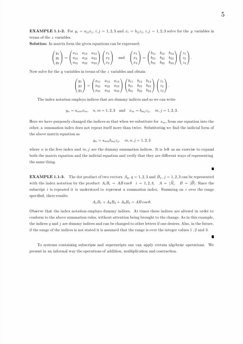
EXAMPLE 1.1-2. For yi = aijxj , i, j = 1, 2, 3 and xi = bijzj , i,j = 1, 2, 3 solve for the y variables in
terms of the z variables.
Solution: In matrix form the given equations can be expressed:
y1
y2
y3
=
a11 a12 a13
a21 a22 a23
a31 a32 a33
x1
x2
x3
and
x1
x2
x3
=
b11 b12 b13
b21 b22 b23
b31 b32 b33
z1
z2
z3
.
Now solve for the y variables in terms of the z variables and obtain y1
y2
y3
=
a11 a12 a13
a21 a22 a23
a31 a32 a33
b11 b12 b13
b21 b22 b23
b31 b32 b33
z1
z2
z3
.
The index notation employs indices that are dummy indices and so we can write
yn = anmxm, n, m = 1, 2, 3 and xm = bmjzj , m, j = 1, 2, 3.
Here we have purposely changed the indices so that when we substitute for xm, from one equation into the
other, a summation index does not repeat itself more than twice. Substituting we find the indicial form of
the above matrix equation as
yn = anmbmjzj , m, n, j = 1, 2, 3
where n is the free index and m, j are the dummy summation indices. It is left as an exercise to expand
both the matrix equation and the indicial equation and verify that they are different ways of representing
the same thing.
EXAMPLE 1.1-3. The dot product of two vectors Aq, q = 1, 2, 3 and Bj , j = 1, 2, 3 can be represented
with the index notation by the product AiBi = AB cos θ i = 1, 2, 3, A = | A|, B = | B|. Since the
subscript i is repeated it is understood to represent a summation index. Summing on i over the range
specified, there results
A1B1 + A2B2 + A3B3 = AB cos θ.
Observe that the index notation employs dummy indices. At times these indices are altered in order to
conform to the above summation rules, without attention being brought to the change. As in this example,
the indices q and j are dummy indices and can be changed to other letters if one desires. Also, in the future,
if the range of the indices is not stated it is assumed that the range is over the integer values 1 , 2 and 3.
To systems containing subscripts and superscripts one can apply certain algebraic operations. We
present in an informal way the operations of addition, multiplication and contraction.

8/6/2019 Introduction to Tensor Calculus Continuum Mechanics - J. Heinbockel
http://slidepdf.com/reader/full/introduction-to-tensor-calculus-continuum-mechanics-j-heinbockel 10/372
6
Addition, Multiplication and Contraction
The algebraic operation of addition or subtraction applies to systems of the same type and order. That
is we can add or subtract like components in systems. For example, the sum of Aijk and Bi
jk is again a
system of the same type and is denoted by C ijk = Aijk + Bi
jk, where like components are added.
The product of two systems is obtained by multiplying each component of the first system with each
component of the second system. Such a product is called an outer product. The order of the resulting
product system is the sum of the orders of the two systems involved in forming the product. For example,
if Aij is a second order system and Bmnl is a third order system, with all indices having the range 1 to N,
then the product system is fifth order and is denoted C imnlj = Ai
jBmnl. The product system represents N 5
terms constructed from all possible products of the components from Aij with the components from Bmnl.
The operation of contraction occurs when a lower index is set equal to an upper index and the summation
convention is invoked. For example, if we have a fifth order system C imnlj and we set i = j and sum, then
we form the system
C mnl = C jmnlj = C 1mnl
1 + C 2mnl2 + · · · + C Nmnl
N .
Here the symbol C mnl is used to represent the third order system that results when the contraction is
performed. Whenever a contraction is performed, the resulting system is always of order 2 less than the
original system. Under certain special conditions it is permissible to perform a contraction on two lower case
indices. These special conditions will be considered later in the section.
The above operations will be more formally defined after we have explained what tensors are.
The e-permutation symbol and Kronecker delta
Two symbols that are used quite frequently with the indicial notation are the e-permutation symbol
and the Kronecker delta. The e-permutation symbol is sometimes referred to as the alternating tensor. The
e-permutation symbol, as the name suggests, deals with permutations. A permutation is an arrangement of
things. When the order of the arrangement is changed, a new permutation results. A transposition is an
interchange of two consecutive terms in an arrangement. As an example, let us change the digits 1 2 3 to
3 2 1 by making a sequence of transpositions. Starting with the digits in the order 1 2 3 we interchange 2 and
3 (first transposition) to obtain 1 3 2. Next, interchange the digits 1 and 3 ( second transposition) to obtain
3 1 2. Finally, interchange the digits 1 and 2 (third transposition) to achieve 3 2 1. Here the total number
of transpositions of 1 2 3 to 3 2 1 is three, an odd number. Other transpositions of 1 2 3 to 3 2 1 can also be
written. However, these are also an odd number of transpositions.

8/6/2019 Introduction to Tensor Calculus Continuum Mechanics - J. Heinbockel
http://slidepdf.com/reader/full/introduction-to-tensor-calculus-continuum-mechanics-j-heinbockel 11/372
7
EXAMPLE 1.1-4. The total number of possible ways of arranging the digits 1 2 3 is six. We have
three choices for the first digit. Having chosen the first digit, there are only two choices left for the second
digit. Hence the remaining number is for the last digit. The product (3)(2)(1) = 3! = 6 is the number of
permutations of the digits 1, 2 and 3. These six permutations are
1 2 3 even permutation1 3 2 odd permutation
3 1 2 even permutation
3 2 1 odd permutation
2 3 1 even permutation
2 1 3 odd permutation.
Here a permutation of 1 2 3 is called even or odd depending upon whether there is an even or odd number
of transpositions of the digits. A mnemonic device to remember the even and odd permutations of 123
is illustrated in the figure 1.1-1. Note that even permutations of 123 are obtained by selecting any three
consecutive numbers from the sequence 123123 and the odd permutations result by selecting any three
consecutive numbers from the sequence 321321.
Figure 1.1-1. Permutations of 123.
In general, the number of permutations of n things taken m at a time is given by the relation
P (n, m) = n(n − 1)(n − 2) · · · (n − m + 1).
By selecting a subset of m objects from a collection of n objects, m ≤ n, without regard to the ordering is
called a combination of n objects taken m at a time. For example, combinations of 3 numbers taken from
the set 1, 2, 3, 4 are (123), (124), (134), (234). Note that ordering of a combination is not considered. Thatis, the permutations (123), (132), (231), (213), (312), (321) are considered equal. In general, the number of
combinations of n objects taken m at a time is given by C (n, m) = n
m
=
n!
m!(n − m)!where
nm
are the
binomial coefficients which occur in the expansion
(a + b)n =
nm=0
n
m
an−mbm.

8/6/2019 Introduction to Tensor Calculus Continuum Mechanics - J. Heinbockel
http://slidepdf.com/reader/full/introduction-to-tensor-calculus-continuum-mechanics-j-heinbockel 12/372
8
The definition of permutations can be used to define the e-permutation symbol.
Definition: (e-Permutation symbol or alternating tensor)
The e-permutation symbol is defined
eijk...l = eijk...l =
1 if i j k . . . l is an even permutation of the integers 123 . . . n−1 if i j k . . . l is an odd permutation of the integers 123 . . . n
0 in all other cases
EXAMPLE 1.1-5. Find e612453.
Solution: To determine whether 612453 is an even or odd permutation of 123456 we write down the given
numbers and below them we write the integers 1 through 6. Like numbers are then connected by a line and
we obtain figure 1.1-2.
Figure 1.1-2. Permutations of 123456.
In figure 1.1-2, there are seven intersections of the lines connecting like numbers. The number of
intersections is an odd number and shows that an odd number of transpositions must be performed. These
results imply e612453 = −1.
Another definition used quite frequently in the representation of mathematical and engineering quantities
is the Kronecker delta which we now define in terms of both subscripts and superscripts.
Definition: (Kronecker delta) The Kronecker delta is defined:
δij = δji =
1 if i equals j
0 if i is different from j

8/6/2019 Introduction to Tensor Calculus Continuum Mechanics - J. Heinbockel
http://slidepdf.com/reader/full/introduction-to-tensor-calculus-continuum-mechanics-j-heinbockel 13/372

8/6/2019 Introduction to Tensor Calculus Continuum Mechanics - J. Heinbockel
http://slidepdf.com/reader/full/introduction-to-tensor-calculus-continuum-mechanics-j-heinbockel 14/372
10
as δKK represents a single term because of the capital letters. Another notation which is used to denote no
summation of the indices is to put parenthesis about the indices which are not to be summed. For example,
a(k)jδ(k)(k) = akj,
since δ(k)(k) represents a single term and the parentheses indicate that no summation is to be performed.At any time we may employ either the underscore notation, the capital letter notation or the parenthesis
notation to denote that no summation of the indices is to be performed. To avoid confusion altogether, one
can write out parenthetical expressions such as “(no summation on k)”.
EXAMPLE 1.1-8. In the Kronecker delta symbol δij we set j equal to i and perform a summation. This
operation is called a contraction. There results δii , which is to be summed over the range of the index i.
Utilizing the range 1, 2, . . . , N we have
δii = δ11 + δ2
2 + · · · + δN N
δii = 1 + 1 + · · · + 1
δii = N.
In three dimension we have δij , i, j = 1, 2, 3 and
δkk = δ11 + δ2
2 + δ33 = 3.
In certain circumstances the Kronecker delta can be written with only subscripts. For example,
δij, i, j = 1, 2, 3. We shall find that these circumstances allow us to perform a contraction on the lower
indices so that δii = 3.
EXAMPLE 1.1-9. The determinant of a matrix A = (aij) can be represented in the indicial notation.
Employing the e-permutation symbol the determinant of an N × N matrix is expressed
|A| = eij...ka1ia2j · · · aNk
where eij...k is an N th order system. In the special case of a 2 × 2 matrix we write
|A| = eija1ia2j
where the summation is over the range 1,2 and the e-permutation symbol is of order 2. In the special caseof a 3 × 3 matrix we have
|A| =
a11 a12 a13
a21 a22 a23
a31 a32 a33
= eijkai1aj2ak3 = eijka1ia2ja3k
where i,j,k are the summation indices and the summation is over the range 1,2,3. Here eijk denotes the
e-permutation symbol of order 3. Note that by interchanging the rows of the 3 × 3 matrix we can obtain
8/6/2019 Introduction to Tensor Calculus Continuum Mechanics - J. Heinbockel
http://slidepdf.com/reader/full/introduction-to-tensor-calculus-continuum-mechanics-j-heinbockel 15/372
11
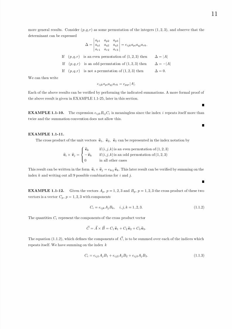
more general results. Consider ( p,q,r) as some permutation of the integers (1, 2, 3), and observe that the
determinant can be expressed
∆ =
a p1 a p2 a p3
aq1 aq2 aq3
ar1 ar2 ar3
= eijka piaqjark.
If ( p,q,r) is an even permutation of (1, 2, 3) then ∆ = |A|If ( p,q,r) is an odd permutation of (1, 2, 3) then ∆ = −|A|If ( p,q,r) is not a permutation of (1, 2, 3) then ∆ = 0.
We can then write
eijka piaqjark = e pqr|A|.
Each of the above results can be verified by performing the indicated summations. A more formal proof of
the above result is given in EXAMPLE 1.1-25, later in this section.
EXAMPLE 1.1-10. The expression eijkBijC i is meaningless since the index i repeats itself more than
twice and the summation convention does not allow this.
EXAMPLE 1.1-11.
The cross product of the unit vectors e1, e2, e3 can be represented in the index notation by
ei × ej =
ek if (i,j,k) is an even permutation of (1, 2, 3)
− ek if (i,j,k) is an odd permutation of (1, 2, 3)
0 in all other cases
This result can be written in the form ei × ej = ekij ek. This later result can be verified by summing on the
index k and writing out all 9 possible combinations for i and j.
EXAMPLE 1.1-12. Given the vectors A p, p = 1, 2, 3 and B p, p = 1, 2, 3 the cross product of these two
vectors is a vector C p, p = 1, 2, 3 with components
C i = eijkAjBk, i, j, k = 1, 2, 3. (1.1.2)
The quantities C i represent the components of the cross product vector
C = A×
B = C 1 e1
+ C 2 e2
+ C 3 e3
.
The equation (1.1.2), which defines the components of C , is to be summed over each of the indices which
repeats itself. We have summing on the index k
C i = eij1AjB1 + eij2AjB2 + eij3AjB3. (1.1.3)

8/6/2019 Introduction to Tensor Calculus Continuum Mechanics - J. Heinbockel
http://slidepdf.com/reader/full/introduction-to-tensor-calculus-continuum-mechanics-j-heinbockel 16/372
12
We next sum on the index j which repeats itself in each term of equation (1.1.3). This gives
C i = ei11A1B1 + ei21A2B1 + ei31A3B1
+ ei12A1B2 + ei22A2B2 + ei32A3B2
+ ei13A1B3 + ei23A2B3 + ei33A3B3.
(1.1.4)
Now we are left with i being a free index which can have any of the values of 1 , 2 or 3. Letting i = 1, then
letting i = 2, and finally letting i = 3 produces the cross product components
C 1 = A2B3 − A3B2
C 2 = A3B1 − A1B3
C 3 = A1B2 − A2B1.
The cross product can also be expressed in the form A × B = eijkAjBk ei. This result can be verified by
summing over the indices i, j and k.
EXAMPLE 1.1-13. Show
eijk = −eikj = ejki for i,j,k = 1, 2, 3
Solution: The array i k j represents an odd number of transpositions of the indices i j k and to each
transposition there is a sign change of the e-permutation symbol. Similarly, j k i is an even transposition
of i j k and so there is no sign change of the e-permutation symbol. The above holds regardless of the
numerical values assigned to the indices i,j,k.
The e-δ Identity
An identity relating the e-permutation symbol and the Kronecker delta, which is useful in the simpli-
fication of tensor expressions, is the e-δ identity. This identity can be expressed in different forms. The
subscript form for this identity is
eijkeimn = δjmδkn − δjnδkm, i, j, k, m, n = 1, 2, 3
where i is the summation index and j,k,m,n are free indices. A device used to remember the positions of
the subscripts is given in the figure 1.1-3.
The subscripts on the four Kronecker delta’s on the right-hand side of the e-δ identity then are read
(first)(second)-(outer)(inner).
This refers to the positions following the summation index. Thus, j, m are the first indices after the sum-
mation index and k, n are the second indices after the summation index. The indices j, n are outer indices
when compared to the inner indices k, m as the indices are viewed as written on the left-hand side of the
identity.

8/6/2019 Introduction to Tensor Calculus Continuum Mechanics - J. Heinbockel
http://slidepdf.com/reader/full/introduction-to-tensor-calculus-continuum-mechanics-j-heinbockel 17/372
13
Figure 1.1-3. Mnemonic device for position of subscripts.
Another form of this identity employs both subscripts and superscripts and has the form
eijk
eimn = δj
mδk
n − δj
nδk
m. (1.1.5)
One way of proving this identity is to observe the equation (1.1.5) has the free indices j,k,m,n. Each
of these indices can have any of the values of 1 , 2 or 3. There are 3 choices we can assign to each of j, k, m
or n and this gives a total of 34 = 81 possible equations represented by the identity from equation (1.1.5).
By writing out all 81 of these equations we can verify that the identity is true for all possible combinations
that can be assigned to the free indices.
An alternate proof of the e − δ identity is to consider the determinant
δ11 δ1
2 δ13
δ21 δ2
2 δ23
δ
3
1 δ
3
2 δ
3
3
=
1 0 00 1 0
0 0 1
= 1.
By performing a permutation of the rows of this matrix we can use the permutation symbol and writeδi1 δi2 δi3δj1 δj2 δj3δk1 δk2 δk3
= eijk .
By performing a permutation of the columns, we can writeδir δis δitδjr δjs δjtδkr δks δkt
= eijkerst.
Now perform a contraction on the indices i and r to obtainδii δis δitδji δjs δjtδki δks δkt
= eijkeist.
Summing on i we have δii = δ11 + δ2
2 + δ33 = 3 and expand the determinant to obtain the desired result
δjsδkt − δjt δks = eijkeist.
8/6/2019 Introduction to Tensor Calculus Continuum Mechanics - J. Heinbockel
http://slidepdf.com/reader/full/introduction-to-tensor-calculus-continuum-mechanics-j-heinbockel 18/372
14
Generalized Kronecker delta
The generalized Kronecker delta is defined by the (n × n) determinant
δij...kmn...p =
δim δin · · · δi pδjm δjn · · · δj p
..
.
..
.
. ..
..
.δkm δkn · · · δk p
.
For example, in three dimensions we can write
δijkmnp =
δim δin δi pδjm δjn δj pδkm δkn δk p
= eijkemnp.
Performing a contraction on the indices k and p we obtain the fourth order system
δrsmn = δrspmnp = erspemnp = e prse pmn = δrmδsn − δrnδsm.
As an exercise one can verify that the definition of the e-permutation symbol can also be defined in terms
of the generalized Kronecker delta as
ej1j2j3···jN = δ1 2 3 ···N j1j2j3···jN
.
Additional definitions and results employing the generalized Kronecker delta are found in the exercises.
In section 1.3 we shall show that the Kronecker delta and epsilon permutation symbol are numerical tensors
which have fixed components in every coordinate system.
Additional Applications of the Indicial Notation
The indicial notation, together with the e − δ identity, can be used to prove various vector identities.
EXAMPLE 1.1-14. Show, using the index notation, that A × B = − B × ASolution: Let
C = A × B = C 1 e1 + C 2 e2 + C 3 e3 = C i ei and let
D = B × A = D1 e1 + D2 e2 + D3 e3 = Di ei.We have shown that the components of the cross products can be represented in the index notation by
C i = eijkAjBk and Di = eijkBjAk.
We desire to show that Di = −C i for all values of i. Consider the following manipulations: Let Bj = Bsδsj
and Ak = Amδmk and write
Di = eijkBjAk = eijkBsδsjAmδmk (1.1.6)
where all indices have the range 1, 2, 3. In the expression (1.1.6) note that no summation index appears
more than twice because if an index appeared more than twice the summation convention would become
meaningless. By rearranging terms in equation (1.1.6) we have
Di = eijkδsjδmkBsAm = eismBsAm.
8/6/2019 Introduction to Tensor Calculus Continuum Mechanics - J. Heinbockel
http://slidepdf.com/reader/full/introduction-to-tensor-calculus-continuum-mechanics-j-heinbockel 19/372
15
In this expression the indices s and m are dummy summation indices and can be replaced by any other
letters. We replace s by k and m by j to obtain
Di = eikjAjBk = −eijkAjBk = −C i.
Consequently, we find that D = −
C or
B ×
A = −
A ×
B. That is,
D = Di ei = −C i ei = −
C.
Note 1. The expressions
C i = eijkAjBk and C m = emnpAnB p
with all indices having the range 1, 2, 3, appear to be different because different letters are used as sub-
scripts. It must be remembered that certain indices are summed according to the summation convention
and the other indices are free indices and can take on any values from the assigned range. Thus, after
summation, when numerical values are substituted for the indices involved, none of the dummy letters
used to represent the components appear in the answer.
Note 2. A second important point is that when one is working with expressions involving the index notation,
the indices can be changed directly. For example, in the above expression for Di we could have replaced
j by k and k by j simultaneously (so that no index repeats itself more than twice) to obtain
Di = eijkBjAk = eikjBkAj = −eijkAjBk = −C i.
Note 3. Be careful in switching back and forth between the vector notation and index notation. Observe that a
vector A can be represented
A = Ai eior its components can be represented
A
· ei = Ai, i = 1, 2, 3.
Do not set a vector equal to a scalar. That is, do not make the mistake of writing A = Ai as this is a
misuse of the equal sign. It is not possible for a vector to equal a scalar because they are two entirely
different quantities. A vector has both magnitude and direction while a scalar has only magnitude.
EXAMPLE 1.1-15. Verify the vector identity
A · ( B × C ) = B · ( C × A)
Solution: Let
B × C = D = Di ei where Di = eijkBjC k and let
C × A = F = F i ei where F i = eijkC jAk
where all indices have the range 1, 2, 3. To prove the above identity, we have
A · ( B × C ) = A · D = AiDi = AieijkBjC k
= Bj(eijkAiC k)
= Bj(ejkiC kAi)

8/6/2019 Introduction to Tensor Calculus Continuum Mechanics - J. Heinbockel
http://slidepdf.com/reader/full/introduction-to-tensor-calculus-continuum-mechanics-j-heinbockel 20/372
16
since eijk = ejki. We also observe from the expression
F i = eijkC jAk
that we may obtain, by permuting the symbols, the equivalent expression
F j = ejkiC kAi.
This allows us to write
A · ( B × C ) = BjF j = B · F = B · ( C × A)
which was to be shown.
The quantity A · ( B × C ) is called a triple scalar product. The above index representation of the triple
scalar product implies that it can be represented as a determinant (See example 1.1-9). We can write
A
·( B
× C ) =
A1 A2 A3
B1 B2 B3
C 1 C 2 C 3
= eijkAiBjC k
A physical interpretation that can be assigned to this triple scalar product is that its absolute value represents
the volume of the parallelepiped formed by the three noncoplaner vectors A, B, C . The absolute value is
needed because sometimes the triple scalar product is negative. This physical interpretation can be obtained
from an analysis of the figure 1.1-4.
Figure 1.1-4. Triple scalar product and volume
8/6/2019 Introduction to Tensor Calculus Continuum Mechanics - J. Heinbockel
http://slidepdf.com/reader/full/introduction-to-tensor-calculus-continuum-mechanics-j-heinbockel 21/372
17
In figure 1.1-4 observe that: (i) | B × C | is the area of the parallelogram PQRS. (ii) the unit vector
en = B × C
| B × C |
is normal to the plane containing the vectors B and C. (iii) The dot product
A · en =
A · B × C
| B × C |
= h
equals the projection of A on en which represents the height of the parallelepiped. These results demonstrate
that A · ( B × C ) = | B × C | h = (area of base)(height) = volume.
EXAMPLE 1.1-16. Verify the vector identity
( A × B) × ( C × D) = C ( D · A × B) − D( C · A × B)
Solution: Let F = A × B = F i ei and E = C × D = E i ei. These vectors have the components
F i = eijkAjBk and E m = emnpC nD p
where all indices have the range 1, 2, 3. The vector G = F × E = Gi ei has the components
Gq = eqimF iE m = eqimeijkemnpAjBkC nD p.
From the identity eqim = emqi this can be expressed
Gq = (emqiemnp)eijkAjBkC nD p
which is now in a form where we can use the e − δ identity applied to the term in parentheses to produce
Gq = (δqnδip − δqpδin)eijkAjBkC nD p.
Simplifying this expression we have:
Gq = eijk [(D pδip)(C nδqn)AjBk − (D pδqp)(C nδin)AjBk]
= eijk [DiC qAjBk − DqC iAjBk]
= C q [DieijkAjBk] − Dq [C ieijkAjBk]
which are the vector components of the vector
C ( D · A × B) − D( C · A × B).

8/6/2019 Introduction to Tensor Calculus Continuum Mechanics - J. Heinbockel
http://slidepdf.com/reader/full/introduction-to-tensor-calculus-continuum-mechanics-j-heinbockel 22/372
18
Transformation Equations
Consider two sets of N independent variables which are denoted by the barred and unbarred symbols
xi and xi with i = 1, . . . , N . The independent variables xi, i = 1, . . . , N can be thought of as defining
the coordinates of a point in a N −dimensional space. Similarly, the independent barred variables define a
point in some other N −dimensional space. These coordinates are assumed to be real quantities and are notcomplex quantities. Further, we assume that these variables are related by a set of transformation equations.
xi = xi(x1, x2, . . . , xN ) i = 1, . . . , N . (1.1.7)
It is assumed that these transformation equations are independent. A necessary and sufficient condition that
these transformation equations be independent is that the Jacobian determinant be different from zero, that
is
J (x
x) =
∂xi
∂ xj
=
∂x1
∂x1∂x1
∂x2· · · ∂x1
∂xN
∂x2
∂x1∂x2
∂x2· · · ∂x2
∂xN
......
. . ....
∂xN∂x1
∂xN∂x2
· · · ∂xN∂xN
= 0.
This assumption allows us to obtain a set of inverse relations
xi = xi(x1, x2, . . . , xN ) i = 1, . . . , N , (1.1.8)
where the xs are determined in terms of the xs. Throughout our discussions it is to be understood that the
given transformation equations are real and continuous. Further all derivatives that appear in our discussions
are assumed to exist and be continuous in the domain of the variables considered.
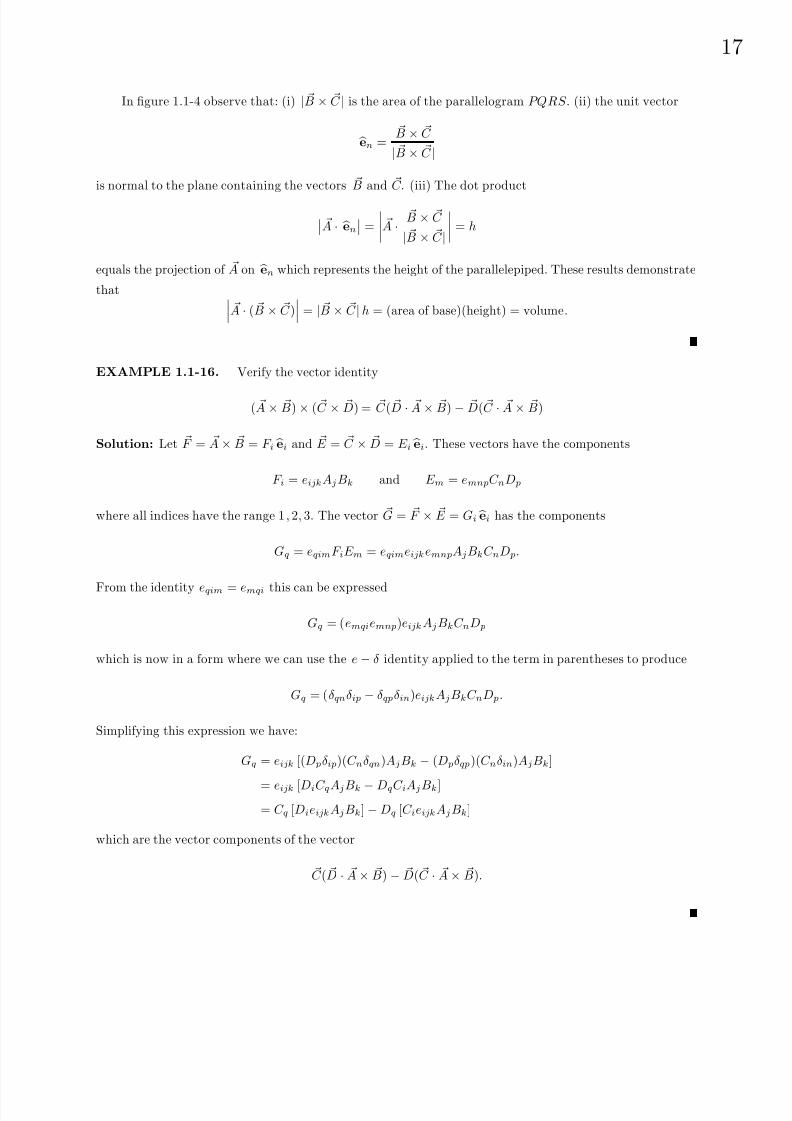
EXAMPLE 1.1-17. The following is an example of a set of transformation equations of the form
defined by equations (1.1.7) and (1.1.8) in the case N = 3. Consider the transformation from cylindricalcoordinates (r,α,z) to spherical coordinates (ρ, β, α). From the geometry of the figure 1.1-5 we can find the
transformation equationsr = ρ sin β
α = α 0 < α < 2π
z = ρ cos β 0 < β < π
with inverse transformationρ =
r2 + z2
α = α
β = arctan(r
z
)
Now make the substitutions
(x1, x2, x3) = (r,α,z) and (x1, x2, x3) = (ρ, β, α).
8/6/2019 Introduction to Tensor Calculus Continuum Mechanics - J. Heinbockel
http://slidepdf.com/reader/full/introduction-to-tensor-calculus-continuum-mechanics-j-heinbockel 23/372
19
Figure 1.1-5. Cylindrical and Spherical Coordinates
The resulting transformations then have the forms of the equations (1.1.7) and (1.1.8).
Calculation of Derivatives
We now consider the chain rule applied to the differentiation of a function of the bar variables. We
represent this differentiation in the indicial notation. Let Φ = Φ(x1, x2, . . . , xn) be a scalar function of the
variables xi, i = 1, . . . , N and let these variables be related to the set of variables xi, with i = 1, . . . , N by
the transformation equations (1.1.7) and (1.1.8). The partial derivatives of Φ with respect to the variables
xi can be expressed in the indicial notation as
∂ Φ
∂xi=
∂ Φ
∂xj
∂xj
∂xi=
∂ Φ
∂x1
∂x1
∂xi+
∂ Φ
∂x2
∂x2
∂xi+ · · · +
∂ Φ
∂xN
∂xN
∂xi(1.1.9)
for any fixed value of i satisfying 1 ≤ i ≤ N.
The second partial derivatives of Φ can also be expressed in the index notation. Differentiation of
equation (1.1.9) partially with respect to xm produces
∂ 2Φ
∂xi∂xm=
∂ Φ
∂xj
∂ 2xj
∂xi∂xm+
∂
∂xm
∂ Φ
∂xj
∂xj
∂xi. (1.1.10)
This result is nothing more than an application of the general rule for differentiating a product of two
quantities. To evaluate the derivative of the bracketed term in equation (1.1.10) it must be remembered that
the quantity inside the brackets is a function of the bar variables. Let
G =∂ Φ
∂xj= G(x1, x2, . . . , xN )
to emphasize this dependence upon the bar variables, then the derivative of G is
∂G
∂xm=
∂G
∂xk
∂xk
∂xm=
∂ 2Φ
∂xj∂xk
∂xk
∂xm. (1.1.11)
This is just an application of the basic rule from equation (1.1.9) with Φ replaced by G. Hence the derivative
from equation (1.1.10) can be expressed
∂ 2Φ
∂xi∂xm=
∂ Φ
∂xj
∂ 2xj
∂xi∂xm+
∂ 2Φ
∂xj∂xk
∂xj
∂xi
∂xk
∂xm(1.1.12)
where i, m are free indices and j, k are dummy summation indices.
8/6/2019 Introduction to Tensor Calculus Continuum Mechanics - J. Heinbockel
http://slidepdf.com/reader/full/introduction-to-tensor-calculus-continuum-mechanics-j-heinbockel 24/372
20
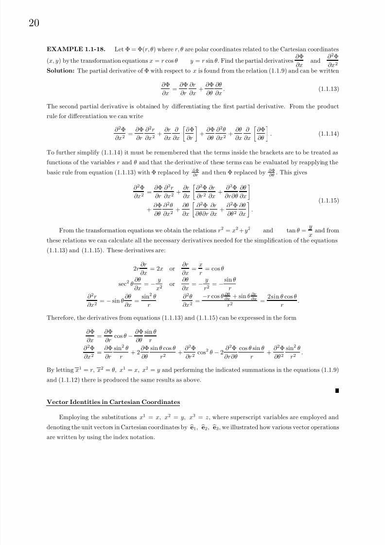
EXAMPLE 1.1-18. Let Φ = Φ(r, θ) where r, θ are polar coordinates related to the Cartesian coordinates
(x, y) by the transformation equations x = r cos θ y = r sin θ. Find the partial derivatives∂ Φ
∂xand
∂ 2Φ
∂x2
Solution: The partial derivative of Φ with respect to x is found from the relation (1.1.9) and can be written
∂ Φ
∂x
=∂ Φ
∂r
∂r
∂x
+∂ Φ
∂θ
∂θ
∂x
. (1.1.13)
The second partial derivative is obtained by differentiating the first partial derivative. From the product
rule for differentiation we can write
∂ 2Φ
∂x2=
∂ Φ
∂r
∂ 2r
∂x2+
∂r
∂x
∂
∂x
∂ Φ
∂r
+
∂ Φ
∂θ
∂ 2θ
∂x2+
∂θ
∂x
∂
∂x
∂ Φ
∂θ
. (1.1.14)
To further simplify (1.1.14) it must be remembered that the terms inside the brackets are to be treated as
functions of the variables r and θ and that the derivative of these terms can be evaluated by reapplying the
basic rule from equation (1.1.13) with Φ replaced by ∂ Φ∂r
and then Φ replaced by ∂ Φ∂θ
. This gives
∂
2
Φ∂x2 = ∂ Φ∂r ∂
2
r∂x2 + ∂r∂x ∂
2
Φ∂r2 ∂r∂x + ∂
2
Φ∂r∂θ ∂θ∂x +
∂ Φ
∂θ
∂ 2θ
∂x2+
∂θ
∂x
∂ 2Φ
∂θ∂r
∂r
∂x+
∂ 2Φ
∂θ2
∂θ
∂x
.
(1.1.15)
From the transformation equations we obtain the relations r2 = x2 + y2 and tan θ =y
xand from
these relations we can calculate all the necessary derivatives needed for the simplification of the equations
(1.1.13) and (1.1.15). These derivatives are:
2r∂r
∂x= 2x or
∂r
∂x=
x
r= cos θ
sec
2
θ
∂θ
∂x = −y
x2 or
∂θ
∂x = −y
r2 = −sin θ
r∂ 2r
∂x2= − sin θ
∂θ
∂x=
sin2 θ
r
∂ 2θ
∂x2=
−r cos θ ∂θ∂x
+ sin θ ∂r∂x
r2=
2sin θ cos θ
r.
Therefore, the derivatives from equations (1.1.13) and (1.1.15) can be expressed in the form
∂ Φ
∂x=
∂ Φ
∂rcos θ − ∂ Φ
∂θ
sin θ
r
∂ 2Φ
∂x2=
∂ Φ
∂r
sin2 θ
r+ 2
∂ Φ
∂θ
sin θ cos θ
r2+
∂ 2Φ
∂r2cos2 θ − 2
∂ 2Φ
∂r∂θ
cos θ sin θ
r+
∂ 2Φ
∂θ 2
sin2 θ
r2.
By letting x1 = r, x2 = θ, x1 = x, x2 = y and performing the indicated summations in the equations (1.1.9)
and (1.1.12) there is produced the same results as above.
Vector Identities in Cartesian Coordinates
Employing the substitutions x1 = x, x2 = y, x3 = z, where superscript variables are employed and
denoting the unit vectors in Cartesian coordinates by e1, e2, e3, we illustrated how various vector operations
are written by using the index notation.

8/6/2019 Introduction to Tensor Calculus Continuum Mechanics - J. Heinbockel
http://slidepdf.com/reader/full/introduction-to-tensor-calculus-continuum-mechanics-j-heinbockel 25/372
21
Gradient. In Cartesian coordinates the gradient of a scalar field is
grad φ =∂φ
∂xe1 +
∂φ
∂ye2 +
∂φ
∂ze3.
The index notation focuses attention only on the components of the gradient. In Cartesian coordinates these
components are represented using a comma subscript to denote the derivative
ej · grad φ = φ,j =∂φ
∂xj, j = 1, 2, 3.
The comma notation will be discussed in section 4. For now we use it to denote derivatives. For example
φ ,j =∂φ
∂xj, φ ,jk =
∂ 2φ
∂xj∂xk, etc.
Divergence. In Cartesian coordinates the divergence of a vector field A is a scalar field and can be
represented
∇ · A = div A =∂A1
∂x+
∂A2
∂y+
∂A3
∂z.
Employing the summation convention and index notation, the divergence in Cartesian coordinates can be
represented
∇ · A = div A = Ai,i =∂Ai
∂xi=
∂A1
∂x1+
∂A2
∂x2+
∂A3
∂x3
where i is the dummy summation index.
Curl. To represent the vector B = curl A = ∇ × A in Cartesian coordinates, we note that the index
notation focuses attention only on the components of this vector. The components Bi, i = 1, 2, 3 of B can
be represented
Bi =
ei · curl A = eijkAk,j , for i,j,k = 1, 2, 3
where eijk is the permutation symbol introduced earlier and Ak,j =∂Ak
∂xj . To verify this representation of thecurl A we need only perform the summations indicated by the repeated indices. We have summing on j that
Bi = ei1kAk,1 + ei2kAk,2 + ei3kAk,3.
Now summing each term on the repeated index k gives us
Bi = ei12A2,1 + ei13A3,1 + ei21A1,2 + ei23A3,2 + ei31A1,3 + ei32A2,3
Here i is a free index which can take on any of the values 1 , 2 or 3. Consequently, we have
For i = 1, B1 = A3,2 − A2,3 =∂A
3∂x2 −
∂A2
∂x3
For i = 2, B2 = A1,3 − A3,1 =∂A1
∂x3− ∂A3
∂x1
For i = 3, B3 = A2,1 − A1,2 =∂A2
∂x1− ∂A1
∂x2
which verifies the index notation representation of curl A in Cartesian coordinates.
8/6/2019 Introduction to Tensor Calculus Continuum Mechanics - J. Heinbockel
http://slidepdf.com/reader/full/introduction-to-tensor-calculus-continuum-mechanics-j-heinbockel 26/372
22
Other Operations. The following examples illustrate how the index notation can be used to represent
additional vector operators in Cartesian coordinates.
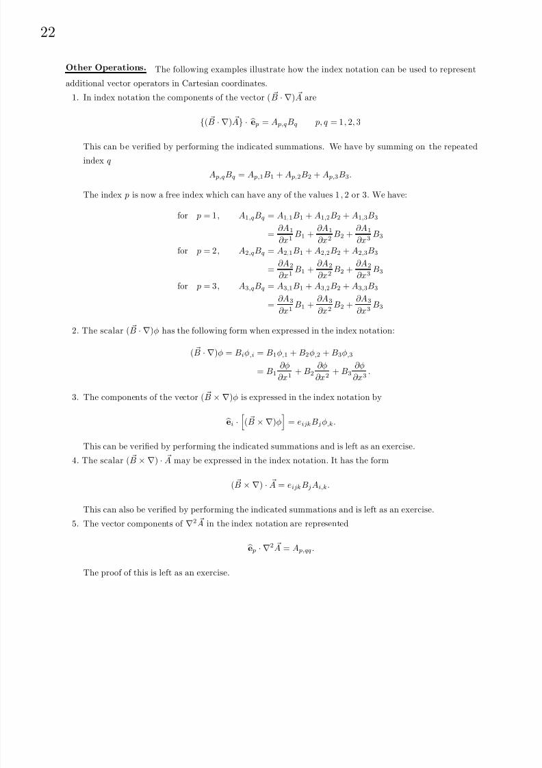
1. In index notation the components of the vector ( B · ∇) A are
( B · ∇) A ·e p = A p,qBq p, q = 1, 2, 3
This can be verified by performing the indicated summations. We have by summing on the repeated
index q
A p,qBq = A p,1B1 + A p,2B2 + A p,3B3.
The index p is now a free index which can have any of the values 1, 2 or 3. We have:
for p = 1, A1,qBq = A1,1B1 + A1,2B2 + A1,3B3
=∂A1
∂x1B1 +
∂A1
∂x2B2 +
∂A1
∂x3B3
for p = 2, A2,qBq = A2,1B1 + A2,2B2 + A2,3B3
=∂A2
∂x1 B1 +∂A2
∂x2 B2 +∂A2
∂x3 B3
for p = 3, A3,qBq = A3,1B1 + A3,2B2 + A3,3B3
=∂A3
∂x1B1 +
∂A3
∂x2B2 +
∂A3
∂x3B3
2. The scalar ( B · ∇)φ has the following form when expressed in the index notation:
( B · ∇)φ = Biφ,i = B1φ,1 + B2φ,2 + B3φ,3
= B1∂φ
∂x1+ B2
∂φ
∂x2+ B3
∂φ
∂x3.
3. The components of the vector ( B× ∇
)φ is expressed in the index notation by
ei ·
( B × ∇)φ
= eijkBjφ,k.
This can be verified by performing the indicated summations and is left as an exercise.
4. The scalar ( B × ∇) · A may be expressed in the index notation. It has the form
( B × ∇) · A = eijkBjAi,k.
This can also be verified by performing the indicated summations and is left as an exercise.
5. The vector components of ∇2 A in the index notation are represented
e p · ∇2 A = A p,qq.
The proof of this is left as an exercise.
8/6/2019 Introduction to Tensor Calculus Continuum Mechanics - J. Heinbockel
http://slidepdf.com/reader/full/introduction-to-tensor-calculus-continuum-mechanics-j-heinbockel 27/372
23
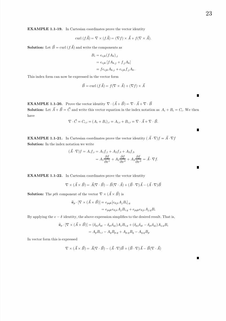
EXAMPLE 1.1-19. In Cartesian coordinates prove the vector identity
curl (f A) = ∇ × (f A) = (∇f ) × A + f (∇ × A).
Solution: Let B = curl (f A) and write the components as
Bi = eijk(f Ak),j
= eijk [f Ak,j + f ,jAk]
= f eijkAk,j + eijkf ,jAk .
This index form can now be expressed in the vector form
B = curl (f A) = f (∇ × A) + (∇f ) × A
EXAMPLE 1.1-20. Prove the vector identity ∇ · ( A + B) = ∇ · A + ∇ · B
Solution: Let A + B = C and write this vector equation in the index notation as Ai + Bi = C i. We then
have
∇ · C = C i,i = (Ai + Bi),i = Ai,i + Bi,i = ∇ · A + ∇ · B.
EXAMPLE 1.1-21. In Cartesian coordinates prove the vector identity ( A · ∇)f = A · ∇f
Solution: In the index notation we write
( A · ∇)f = Aif ,i = A1f ,1 + A2f ,2 + A3f ,3
= A1∂f
∂x1+ A2
∂f
∂x2+ A3
∂f
∂x3= A · ∇f.
EXAMPLE 1.1-22. In Cartesian coordinates prove the vector identity
∇ × ( A × B) = A(∇ · B) − B(∇ · A) + ( B · ∇) A − ( A · ∇) B
Solution: The pth component of the vector ∇ × ( A × B) is
e p · [∇ × ( A × B)] = e pqk[ekjiAjBi],q
= e pqkekjiAjBi,q + e pqkekjiAj,qBi
By applying the e − δ identity, the above expression simplifies to the desired result. That is,
e p · [∇ × ( A × B)] = (δ pjδqi − δ piδqj)AjBi,q + (δ pjδqi − δ piδqj)Aj,qBi
= A pBi,i − AqB p,q + A p,qBq − Aq,qB p
In vector form this is expressed
∇ × ( A × B) = A(∇ · B) − ( A · ∇) B + ( B · ∇) A − B(∇ · A)

8/6/2019 Introduction to Tensor Calculus Continuum Mechanics - J. Heinbockel
http://slidepdf.com/reader/full/introduction-to-tensor-calculus-continuum-mechanics-j-heinbockel 28/372
24
EXAMPLE 1.1-23. In Cartesian coordinates prove the vector identity ∇ × (∇ × A) = ∇(∇ · A) − ∇2 A
Solution: We have for the ith component of ∇× A is given by ei · [∇× A] = eijkAk,j and consequently the
pth component of ∇ × (∇ × A) is
e p · [∇ × (∇ × A)] = e pqr[erjkAk,j ],q
= e pqrerjkAk,jq.
The e − δ identity produces
e p · [∇ × (∇ × A)] = (δ pjδqk − δ pkδqj)Ak,jq
= Ak,pk − A p,qq .
Expressing this result in vector form we have ∇ × (∇ × A) = ∇(∇ · A) − ∇2 A.
Indicial Form of Integral Theorems
The divergence theorem, in both vector and indicial notation, can be written V
div · F dτ =
S
F · n dσ
V
F i,i dτ =
S
F ini dσ i = 1, 2, 3 (1.1.16)
where ni are the direction cosines of the unit exterior normal to the surface, dτ is a volume element and dσ
is an element of surface area. Note that in using the indicial notation the volume and surface integrals are
to be extended over the range specified by the indices. This suggests that the divergence theorem can be
applied to vectors in n−dimensional spaces.
The vector form and indicial notation for the Stokes theorem are
S(∇ × F ) · n dσ = C F · dr S eijkF k,jni dσ = C F i dxi
i,j,k = 1, 2, 3 (1.1.17)
and the Green’s theorem in the plane, which is a special case of the Stoke’s theorem, can be expressed ∂F 2∂x
− ∂F 1∂y
dxdy =
C
F 1 dx + F 2 dy
S
e3jkF k,j dS =
C
F i dxi i,j,k = 1, 2 (1.1.18)
Other forms of the above integral theorems are V
∇φ dτ =
S
φ n dσ
obtained from the divergence theorem by letting F = φ C where C is a constant vector. By replacing F by
F × C in the divergence theorem one can derive V
∇ × F
dτ = −
S
F × n dσ.
In the divergence theorem make the substitution F = φ∇ψ to obtain V
(φ∇2ψ + (∇φ) · (∇ψ)
dτ =
S
(φ∇ψ) · n dσ.
8/6/2019 Introduction to Tensor Calculus Continuum Mechanics - J. Heinbockel
http://slidepdf.com/reader/full/introduction-to-tensor-calculus-continuum-mechanics-j-heinbockel 29/372
25
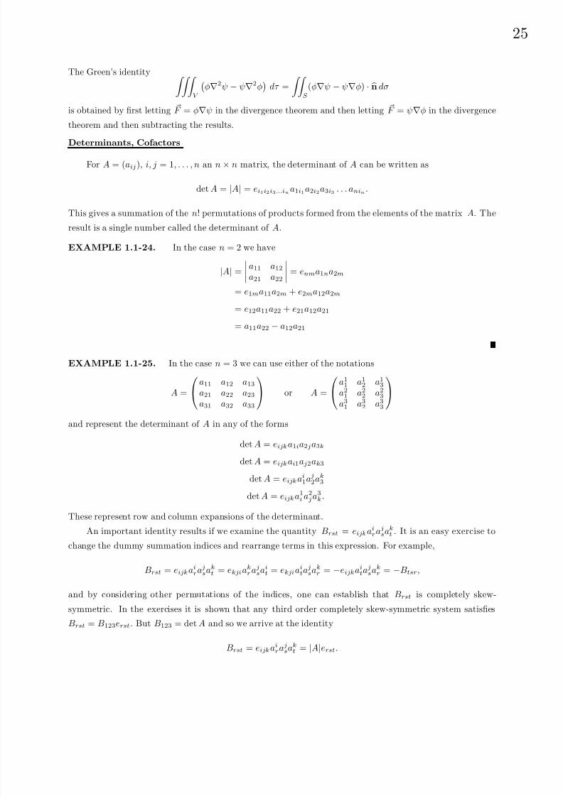
The Green’s identity V
φ∇2ψ − ψ∇2φ
dτ =
S
(φ∇ψ − ψ∇φ) · n dσ
is obtained by first letting F = φ∇ψ in the divergence theorem and then letting F = ψ∇φ in the divergence
theorem and then subtracting the results.
Determinants, Cofactors
For A = (aij), i, j = 1, . . . , n an n × n matrix, the determinant of A can be written as
det A = |A| = ei1i2i3...ina1i1a2i2a3i3 . . . anin .
This gives a summation of the n! permutations of products formed from the elements of the matrix A. The
result is a single number called the determinant of A.
EXAMPLE 1.1-24. In the case n = 2 we have
|A
|=
a11 a12
a21 a22 = enma1na2m
= e1ma11a2m + e2ma12a2m
= e12a11a22 + e21a12a21
= a11a22 − a12a21
EXAMPLE 1.1-25. In the case n = 3 we can use either of the notations
A =
a11 a12 a13
a21 a22 a23
a31 a32 a33
or A =
a1
1 a12 a1
3
a21 a2
2 a23
a31 a3
2 a33
and represent the determinant of A in any of the forms
det A = eijka1ia2ja3k
det A = eijkai1aj2ak3
det A = eijkai1aj2ak3
det A = eijka1i a2
ja3k.
These represent row and column expansions of the determinant.
An important identity results if we examine the quantity Brst = eijkairajsakt . It is an easy exercise to
change the dummy summation indices and rearrange terms in this expression. For example,
Brst = eijkairajsakt = ekjiakrajsait = ekjiaitajsakr = −eijkaita
jsakr = −Btsr,
and by considering other permutations of the indices, one can establish that Brst is completely skew-
symmetric. In the exercises it is shown that any third order completely skew-symmetric system satisfies
Brst = B123erst. But B123 = det A and so we arrive at the identity
Brst = eijkairajsakt = |A|erst.

8/6/2019 Introduction to Tensor Calculus Continuum Mechanics - J. Heinbockel
http://slidepdf.com/reader/full/introduction-to-tensor-calculus-continuum-mechanics-j-heinbockel 30/372

8/6/2019 Introduction to Tensor Calculus Continuum Mechanics - J. Heinbockel
http://slidepdf.com/reader/full/introduction-to-tensor-calculus-continuum-mechanics-j-heinbockel 31/372
27
These cofactors are then combined into the single equation
Air =
1
2!δijkrstasjatk (1.1.25)
which represents the cofactor of ari . When the elements from any row (or column) are multiplied by their
corresponding cofactors, and the results summed, we obtain the value of the determinant. Whenever theelements from any row (or column) are multiplied by the cofactor elements from a different row (or column),
and the results summed, we get zero. This can be illustrated by considering the summation
amr Aim =
1
2!δijkmsta
sjatkamr =
1
2!eijkemsta
mr asjatk
=1
2!eijkerjk |A| =
1
2!δijkrjk |A| = δir|A|
Here we have used the e − δ identity to obtain
δijkrjk = eijkerjk = ejikejrk = δirδkk − δikδkr = 3δir − δir = 2δir
which was used to simplify the above result.
As an exercise one can show that an alternate form of the above summation of elements by its cofactors
is
armAmi = |A|δri .
8/6/2019 Introduction to Tensor Calculus Continuum Mechanics - J. Heinbockel
http://slidepdf.com/reader/full/introduction-to-tensor-calculus-continuum-mechanics-j-heinbockel 32/372
28
EXERCISE 1.1
1. Simplify each of the following by employing the summation property of the Kronecker delta. Perform
sums on the summation indices only if your are unsure of the result.
(a) eijkδkn
(b) eijkδisδjm
(c) eijkδisδjmδkn
(d) aijδin
(e) δijδjn
(f ) δijδjnδni
2. Simplify and perform the indicated summations over the range 1, 2, 3
(a) δii
(b) δijδij
(c) eijkAiAjAk
(d) eijkeijk
(e) eijkδjk
(f ) AiBjδji − BmAnδmn
3. Express each of the following in index notation. Be careful of the notation you use. Note that A = Ai
is an incorrect notation because a vector can not equal a scalar. The notation A · ei = Ai should be used to
express the ith component of a vector.
(a) A · ( B × C )
(b) A × ( B × C )
(c) B( A · C )
(d) B( A · C ) − C ( A · B)
4. Show the e permutation symbol satisfies: (a) eijk = ejki = ekij (b) eijk = −ejik = −eikj = −ekji
5. Use index notation to verify the vector identity A × ( B × C ) = B( A · C ) − C ( A · B)
6. Let yi = aijxj and xm = aimzi where the range of the indices is 1, 2
(a) Solve for yi in terms of zi using the indicial notation and check your result
to be sure that no index repeats itself more than twice.
(b) Perform the indicated summations and write out expressions
for y1, y2 in terms of z1, z2
(c) Express the above equations in matrix form. Expand the matrix
equations and check the solution obtained in part (b).
7. Use the e − δ identity to simplify (a) eijkejik (b) eijkejki
8. Prove the following vector identities:
(a) A · ( B × C ) = B · ( C × A) = C · ( A × B) triple scalar product
(b) ( A × B) × C = B( A · C ) − A( B · C )
9. Prove the following vector identities:
(a) ( A × B) · ( C × D) = ( A · C )( B · D) − ( A · D)( B · C )
(b) A × ( B × C ) + B × ( C × A) + C × ( A × B) = 0
(c) ( A × B) × ( C × D) = B( A · C × D) − A( B · C × D)

8/6/2019 Introduction to Tensor Calculus Continuum Mechanics - J. Heinbockel
http://slidepdf.com/reader/full/introduction-to-tensor-calculus-continuum-mechanics-j-heinbockel 33/372
29
10. For A = (1, −1, 0) and B = (4, −3, 2) find using the index notation,
(a) C i = eijkAjBk, i = 1, 2, 3
(b) AiBi
(c) What do the results in (a) and (b) represent?
11. Represent the differential equationsdy1
dt= a11y1 + a12y2 and
dy2
dt= a21y1 + a22y2
using the index notation.
12.
Let Φ = Φ(r, θ) where r, θ are polar coordinates related to Cartesian coordinates (x, y) by the transfor-
mation equations x = r cos θ and y = r sin θ.
(a) Find the partial derivatives∂ Φ
∂y, and
∂ 2Φ
∂y 2
(b) Combine the result in part (a) with the result from EXAMPLE 1.1-18 to calculate the Laplacian
∇2Φ = ∂ 2
Φ∂x2 + ∂
2
Φ∂y 2
in polar coordinates.
13. (Index notation) Let a11 = 3, a12 = 4, a21 = 5, a22 = 6.
Calculate the quantity C = aijaij , i,j = 1, 2.
14. Show the moments of inertia I ij defined by
I 11 =
R
(y2 + z2)ρ(x, y, z) dτ
I 22 = R
(x2
+ z2
)ρ(x, y, z) dτ
I 33 =
R
(x2 + y2)ρ(x, y, z) dτ
I 23 = I 32 = − R
yzρ(x, y, z) dτ
I 12 = I 21 = − R
xyρ(x, y, z) dτ
I 13 = I 31 = − R
xzρ(x, y, z) dτ,
can be represented in the index notation as I ij =
R
xmxmδij − xixj
ρdτ, where ρ is the density,
x1 = x, x2 = y, x3 = z and dτ = dxdydz is an element of volume.
15. Determine if the following relation is true or false. Justify your answer.
ei
·(
ej
× ek) = (
ei
× ej)
· ek = eijk , i, j, k = 1, 2, 3.
Hint: Let em = (δ1m, δ2m, δ3m).
16. Without substituting values for i, l = 1, 2, 3 calculate all nine terms of the given quantities
(a) Bil = (δijAk + δikAj)ejkl (b) Ail = (δmi Bk + δki Bm)emlk
17. Let Amnxmyn = 0 for arbitrary xi and yi, i = 1, 2, 3, and show that Aij = 0 for all values of i,j.
8/6/2019 Introduction to Tensor Calculus Continuum Mechanics - J. Heinbockel
http://slidepdf.com/reader/full/introduction-to-tensor-calculus-continuum-mechanics-j-heinbockel 34/372
30
18.
(a) For amn, m , n = 1, 2, 3 skew-symmetric, show that amnxmxn = 0.
(b) Let amnxmxn = 0, m, n = 1, 2, 3 for all values of xi, i = 1, 2, 3 and show that amn must be skew-
symmetric.
19. Let A and B denote 3 × 3 matrices with elements aij and bij respectively. Show that if C = AB is a
matrix product, then det(C ) = det(A) · det(B).
Hint: Use the result from example 1.1-9.
20.
(a) Let u1, u2, u3 be functions of the variables s1, s2, s3. Further, assume that s1, s2, s3 are in turn each
functions of the variables x1, x2, x3. Let
∂um
∂xn
=∂ (u1, u2, u3)
∂ (x1, x2, x3)denote the Jacobian of the us with
respect to the xs. Show that
∂ui
∂xm
=
∂ui
∂sj∂sj
∂xm
=
∂ui
∂sj
·
∂sj
∂xm
.
(b) Note that∂xi
∂ xj∂ xj
∂xm=
∂xi
∂xm= δim and show that J (x
x)·J ( x
x) = 1, where J (x
x) is the Jacobian determinant
of the transformation (1.1.7).
21. A third order system amn with ,m,n = 1, 2, 3 is said to be symmetric in two of its subscripts if the
components are unaltered when these subscripts are interchanged. When amn is completely symmetric then
amn = amn = anm = amn = anm = anm. Whenever this third order system is completely symmetric,
then: (i) How many components are there? (ii) How many of these components are distinct?
Hint: Consider the three cases (i) = m = n (ii) = m = n (iii) = m = n.
22. A third order system bmn with ,m,n = 1, 2, 3 is said to be skew-symmetric in two of its subscriptsif the components change sign when the subscripts are interchanged. A completely skew-symmetric third
order system satisfies bmn = −bmn = bmn = −bnm = bnm = −bnm. (i) How many components does
a completely skew-symmetric system have? (ii) How many of these components are zero? (iii) How many
components can be different from zero? (iv) Show that there is one distinct component b123 and that
bmn = emnb123.
Hint: Consider the three cases (i) = m = n (ii) = m = n (iii) = m = n.
23. Let i,j,k = 1, 2, 3 and assume that eijkσjk = 0 for all values of i. What does this equation tell you
about the values σij , i, j = 1, 2, 3?
24. Assume that Amn and Bmn are symmetric for m, n = 1, 2, 3. Let Amnxmxn = Bmnxmxn for arbitrary
values of xi, i = 1, 2, 3, and show that Aij = Bij for all values of i and j.
25. Assume Bmn is symmetric and Bmnxmxn = 0 for arbitrary values of xi, i = 1, 2, 3, show that Bij = 0.

8/6/2019 Introduction to Tensor Calculus Continuum Mechanics - J. Heinbockel
http://slidepdf.com/reader/full/introduction-to-tensor-calculus-continuum-mechanics-j-heinbockel 35/372
31
26. (Generalized Kronecker delta) Define the generalized Kronecker delta as the n×n determinant
δij...kmn...p =
δim δin · · · δi pδjm δjn · · · δj p
......
. . ....
δkm
δkn · · ·
δk p
where δrs is the Kronecker delta.
(a) Show eijk = δ123ijk
(b) Show eijk = δijk123
(c) Show δijmn = eijemn
(d) Define δrsmn = δrspmnp (summation on p)
and show δrsmn = δrmδsn − δrnδsm
Note that by combining the above result with the result from part (c)
we obtain the two dimensional form of the e − δ identity ersemn = δrmδsn − δrnδsm.
(e) Define δr
m =1
2 δrn
mn (summation on n) and show δrst
pst = 2δr
p
(f ) Show δrstrst = 3!
27. Let Air denote the cofactor of ari in the determinant
a1
1 a12 a1
3
a21 a2
2 a23
a31 a3
2 a33
as given by equation (1.1.25).
(a) Show erstAir = eijkasjatk (b) Show erstAr
i = eijkajsakt
28. (a) Show that if Aijk = Ajik , i,j,k = 1, 2, 3 there is a total of 27 elements, but only 18 are distinct.
(b) Show that for i,j,k = 1, 2, . . . , N there are N 3 elements, but only N 2(N + 1)/2 are distinct.
29. Let aij = BiBj for i, j = 1, 2, 3 where B1, B2, B3 are arbitrary constants. Calculate det(aij) = |A|.
30.(a) For A = (aij), i, j = 1, 2, 3, show |A| = eijkai1aj2ak3.
(b) For A = (aij), i,j = 1, 2, 3, show |A| = eijkai1aj2ak3 .
(c) For A = (aij), i,j = 1, 2, 3, show |A| = eijka1i a2
ja3k.
(d) For I = (δij), i,j = 1, 2, 3, show |I | = 1.
31. Let |A| = eijkai1aj2ak3 and define Aim as the cofactor of aim. Show the determinant can beexpressed in any of the forms:
(a) |A| = Ai1ai1 where Ai1 = eijkaj2ak3
(b) |A| = Aj2aj2 where Ai2 = ejikaj1ak3
(c) |A| = Ak3ak3 where Ai3 = ejkiaj1ak2

8/6/2019 Introduction to Tensor Calculus Continuum Mechanics - J. Heinbockel
http://slidepdf.com/reader/full/introduction-to-tensor-calculus-continuum-mechanics-j-heinbockel 36/372
8/6/2019 Introduction to Tensor Calculus Continuum Mechanics - J. Heinbockel
http://slidepdf.com/reader/full/introduction-to-tensor-calculus-continuum-mechanics-j-heinbockel 37/372
33
42. Determine if the following statement is true or false. Justify your answer. eijkAiBjC k = eijkAjBkC i.
43. Let aij, i, j = 1, 2 denote the components of a 2 × 2 matrix A, which are functions of time t.
(a) Expand both |A| = eijai1aj2 and |A| =
a11 a12
a21 a22
to verify that these representations are the same.
(b) Verify the equivalence of the derivative relations
d|A|dt
= eijdai1
dtaj2 + eijai1
daj2
dtand
d|A|dt
=
da11dtda12dt
a21 a22
+
a11 a12da21dt
da22dt
(c) Let aij, i, j = 1, 2, 3 denote the components of a 3 × 3 matrix A, which are functions of time t. Develop
appropriate relations, expand them and verify, similar to parts (a) and (b) above, the representation of
a determinant and its derivative.
44. For f = f (x1, x2, x3) and φ = φ(f ) differentiable scalar functions, use the indicial notation to find a
formula to calculate grad φ .
45. Use the indicial notation to prove (a) ∇ × ∇φ = 0 (b) ∇ · ∇ × A = 0
46. If Aij is symmetric and Bij is skew-symmetric, i, j = 1, 2, 3, then calculate C = AijBij .
47. Assume Aij = Aij(x1, x2, x3) and Aij = Aij(x1, x2, x3) for i, j = 1, 2, 3 are related by the expression
Amn = Aij
∂xi
∂xm
∂xj
∂xn . Calculate the derivative∂Amn
∂xk.
48. Prove that if any two rows (or two columns) of a matrix are interchanged, then the value of the
determinant of the matrix is multiplied by minus one. Construct your proof using 3 × 3 matrices.
49. Prove that if two rows (or columns) of a matrix are proportional, then the value of the determinantof the matrix is zero. Construct your proof using 3 × 3 matrices.
50. Prove that if a row (or column) of a matrix is altered by adding some constant multiple of some other
row (or column), then the value of the determinant of the matrix remains unchanged. Construct your proof
using 3 × 3 matrices.
51. Simplify the expression φ = eijkemnAiAjmAkn.
52. Let Aijk denote a third order system where i,j,k = 1, 2. (a) How many components does this system
have? (b) Let Aijk be skew-symmetric in the last pair of indices, how many independent components does
the system have?
53. Let Aijk denote a third order system where i,j,k = 1, 2, 3. (a) How many components does this
system have? (b) In addition let Aijk = Ajik and Aikj = −Aijk and determine the number of distinct
nonzero components for Aijk .

8/6/2019 Introduction to Tensor Calculus Continuum Mechanics - J. Heinbockel
http://slidepdf.com/reader/full/introduction-to-tensor-calculus-continuum-mechanics-j-heinbockel 38/372
34
54. Show that every second order system T ij can be expressed as the sum of a symmetric system Aij and
skew-symmetric system Bij . Find Aij and Bij in terms of the components of T ij.
55. Consider the system Aijk , i, j, k = 1, 2, 3, 4.
(a) How many components does this system have?
(b) Assume Aijk is skew-symmetric in the last pair of indices, how many independent components does this
system have?
(c) Assume that in addition to being skew-symmetric in the last pair of indices, Aijk + Ajki + Akij = 0 is
satisfied for all values of i,j, and k, then how many independent components does the system have?
56. (a) Write the equation of a line r = r0 + t A in indicial form. (b) Write the equation of the plane
n · (r − r0) = 0 in indicial form. (c) Write the equation of a general line in scalar form. (d) Write the
equation of a plane in scalar form. (e) Find the equation of the line defined by the intersection of the
planes 2x + 3y + 6z = 12 and 6x + 3y + z = 6. (f) Find the equation of the plane through the points
(5, 3, 2),(3, 1, 5),(1, 3, 3). Find also the normal to this plane.
57. The angle 0 ≤ θ ≤ π between two skew lines in space is defined as the angle between their direction
vectors when these vectors are placed at the origin. Show that for two lines with direction numbers ai and
bi i = 1, 2, 3, the cosine of the angle between these lines satisfies
cos θ =aibi√
aiai√
bibi
58. Let aij = −aji for i, j = 1, 2, . . . , N and prove that for N odd det(aij) = 0.
59. Let λ = Aijxixj where Aij = Aji and calculate (a)∂λ
∂xm
(b)∂ 2λ
∂xm∂xk
60. Given an arbitrary nonzero vector U k, k = 1, 2, 3, define the matrix elements aij = eijkU k, where eijk
is the e-permutation symbol. Determine if aij is symmetric or skew-symmetric. Suppose U k is defined by
the above equation for arbitrary nonzero aij, then solve for U k in terms of the aij.
61. If Aij = AiBj = 0 for all i, j values and Aij = Aji for i, j = 1, 2, . . . , N , show that Aij = λBiBj
where λ is a constant. State what λ is.
62. Assume that Aijkm, with i,j,k,m = 1, 2, 3, is completely skew-symmetric. How many independent
components does this quantity have?
63. Consider Rijkm , i, j, k, m = 1, 2, 3, 4. (a) How many components does this quantity have? (b) If Rijkm = −Rijmk = −Rjikm then how many independent components does Rijkm have? (c) If in addition
Rijkm = Rkmij determine the number of independent components.
64. Let xi = aijxj , i, j = 1, 2, 3 denote a change of variables from a barred system of coordinates to an
unbarred system of coordinates and assume that Ai = aijAj where aij are constants, Ai is a function of the
xj variables and Aj is a function of the xj variables. Calculate∂ Ai
∂ xm.
8/6/2019 Introduction to Tensor Calculus Continuum Mechanics - J. Heinbockel
http://slidepdf.com/reader/full/introduction-to-tensor-calculus-continuum-mechanics-j-heinbockel 39/372
35
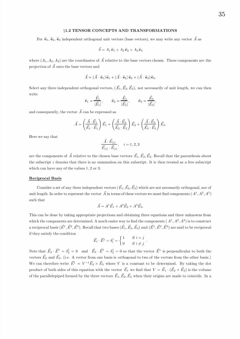
§1.2 TENSOR CONCEPTS AND TRANSFORMATIONS
For e1, e2, e3 independent orthogonal unit vectors (base vectors), we may write any vector A as
A = A1
e1 + A2
e2 + A3
e3
where (A1, A2, A3) are the coordinates of A relative to the base vectors chosen. These components are the
projection of A onto the base vectors and
A = ( A · e1) e1 + ( A · e2) e2 + ( A · e3) e3.
Select any three independent orthogonal vectors, ( E 1, E 2, E 3), not necessarily of unit length, we can then
write e1 = E 1
| E 1|, e2 =
E 2
| E 2|, e3 =
E 3
| E 3|,
and consequently, the vector A can be expressed as
A = A · E 1
E 1 · E 1
E 1 +
A · E 2 E 2 · E 2
E 2 +
A · E 3 E 3 · E 3
E 3.
Here we say that A · E (i)
E (i) · E (i)
, i = 1, 2, 3
are the components of A relative to the chosen base vectors E 1, E 2, E 3. Recall that the parenthesis about
the subscript i denotes that there is no summation on this subscript. It is then treated as a free subscript
which can have any of the values 1, 2 or 3.
Reciprocal Basis
Consider a set of any three independent vectors ( E 1, E 2, E 3) which are not necessarily orthogonal, nor of
unit length. In order to represent the vector A in terms of these vectors we must find components (A1, A2, A3)
such that
A = A1 E 1 + A2 E 2 + A3 E 3.
This can be done by taking appropriate projections and obtaining three equations and three unknowns from
which the components are determined. A much easier way to find the components (A1, A2, A3) is to construct
a reciprocal basis ( E 1, E 2, E 3). Recall that two bases ( E 1, E 2, E 3) and ( E 1, E 2, E 3) are said to be reciprocal
if they satisfy the condition
E i · E j = δji = 1 if i = j
0 if i = j.
Note that E 2 · E 1 = δ12 = 0 and E 3 · E 1 = δ13 = 0 so that the vector E 1 is perpendicular to both the
vectors E 2 and E 3. (i.e. A vector from one basis is orthogonal to two of the vectors from the other basis.)
We can therefore write E 1 = V −1 E 2 × E 3 where V is a constant to be determined. By taking the dot
product of both sides of this equation with the vector E 1 we find that V = E 1 · ( E 2 × E 3) is the volume
of the parallelepiped formed by the three vectors E 1, E 2, E 3 when their origins are made to coincide. In a
8/6/2019 Introduction to Tensor Calculus Continuum Mechanics - J. Heinbockel
http://slidepdf.com/reader/full/introduction-to-tensor-calculus-continuum-mechanics-j-heinbockel 40/372
36
similar manner it can be demonstrated that for ( E 1, E 2, E 3) a given set of basis vectors, then the reciprocal
basis vectors are determined from the relations
E 1 =1
V E 2 × E 3, E 2 =
1
V E 3 × E 1, E 3 =
1
V E 1 × E 2,
where V = E 1 · ( E 2 × E 3) = 0 is a triple scalar product and represents the volume of the parallelepiped
having the basis vectors for its sides.Let ( E 1, E 2, E 3) and ( E 1, E 2, E 3) denote a system of reciprocal bases. We can represent any vector A
with respect to either of these bases. If we select the basis ( E 1, E 2, E 3) and represent A in the form
A = A1 E 1 + A2 E 2 + A3 E 3, (1.2.1)
then the components (A1, A2, A3) of A relative to the basis vectors ( E 1, E 2, E 3) are called the contravariant
components of A. These components can be determined from the equations
A · E 1 = A1, A · E 2 = A2, A · E 3 = A3.
Similarly, if we choose the reciprocal basis ( E 1, E 2, E 3) and represent A in the form
A = A1
E 1 + A2
E 2 + A3
E 3, (1.2.2)
then the components (A1, A2, A3) relative to the basis ( E 1, E 2, E 3) are called the covariant components of
A. These components can be determined from the relations
A · E 1 = A1, A · E 2 = A2, A · E 3 = A3.
The contravariant and covariant components are different ways of representing the same vector with respect
to a set of reciprocal basis vectors. There is a simple relationship between these components which we now
develop. We introduce the notation
E i · E j = gij = gji, and E i · E j = gij = gji (1.2.3)
where gij are called the metric components of the space and gij are called the conjugate metric components
of the space. We can then write
A · E 1 = A1( E 1 · E 1) + A2( E 2 · E 1) + A3( E 3 · E 1) = A1
A · E 1 = A1( E 1 · E 1) + A2( E 2 · E 1) + A3( E 3 · E 1) = A1
or
A1 = A1g11 + A2g12 + A3g13. (1.2.4)
In a similar manner, by considering the dot products A · E 2 and A · E 3 one can establish the results
A2 = A1g21 + A2g22 + A3g23 A3 = A1g31 + A2g32 + A3g33.
These results can be expressed with the index notation as
Ai = gikAk
. (1.2.6)Forming the dot products A · E 1, A · E 2, A · E 3 it can be verified that
Ai = gikAk. (1.2.7)
The equations (1.2.6) and (1.2.7) are relations which exist between the contravariant and covariant compo-
nents of the vector A. Similarly, if for some value j we have E j = α E 1 + β E 2 + γ E 3, then one can show
that E j = gij E i. This is left as an exercise.

8/6/2019 Introduction to Tensor Calculus Continuum Mechanics - J. Heinbockel
http://slidepdf.com/reader/full/introduction-to-tensor-calculus-continuum-mechanics-j-heinbockel 41/372
37
Coordinate Transformations
Consider a coordinate transformation from a set of coordinates (x, y, z) to (u, v, w) defined by a set of
transformation equationsx = x(u, v, w)
y = y(u, v, w)
z = z(u, v, w)
(1.2.8)
It is assumed that these transformations are single valued, continuous and possess the inverse transformation
u = u(x, y, z)
v = v(x, y, z)
w = w(x, y, z).
(1.2.9)
These transformation equations define a set of coordinate surfaces and coordinate curves. The coordinate
surfaces are defined by the equationsu(x, y, z) = c1
v(x, y, z) = c2
w(x, y, z) = c3
(1.2.10)
where c1, c2, c3 are constants. These surfaces intersect in the coordinate curves
r(u, c2, c3), r(c1, v , c3), r(c1, c2, w), (1.2.11)
where
r(u, v, w) = x(u, v, w) e1 + y(u, v, w) e2 + z(u, v, w) e3.
The general situation is illustrated in the figure 1.2-1.
Consider the vectors
E 1 = grad u = ∇u, E 2 = grad v = ∇v, E 3 = grad w = ∇w (1.2.12)
evaluated at the common point of intersection (c1, c2, c3) of the coordinate surfaces. The system of vectors
( E 1, E 2, E 3) can be selected as a system of basis vectors which are normal to the coordinate surfaces.
Similarly, the vectors
E 1 =∂r
∂u, E 2 =
∂r
∂v, E 3 =
∂r
∂w(1.2.13)
when evaluated at the common point of intersection (c1, c2, c3) forms a system of vectors ( E 1, E 2, E 3) which
we can select as a basis. This basis is a set of tangent vectors to the coordinate curves. It is now demonstratedthat the normal basis ( E 1, E 2, E 3) and the tangential basis ( E 1, E 2, E 3) are a set of reciprocal bases.
Recall that r = x e1 + y e2 + z e3 denotes the position vector of a variable point. By substitution for
x, y, z from (1.2.8) there results
r = r(u, v, w) = x(u, v, w) e1 + y(u, v, w) e2 + z(u, v, w) e3. (1.2.14)

8/6/2019 Introduction to Tensor Calculus Continuum Mechanics - J. Heinbockel
http://slidepdf.com/reader/full/introduction-to-tensor-calculus-continuum-mechanics-j-heinbockel 42/372
38
Figure 1.2-1. Coordinate curves and coordinate surfaces.
A small change in r is denoted
dr = dx e1 + dy e2 + dz e3 =∂r
∂udu +
∂r
∂vdv +
∂r
∂wdw (1.2.15)
where∂r
∂u=
∂x
∂u e1 +
∂y
∂u e2 +
∂z
∂u e3
∂r
∂v=
∂x
∂ve1 +
∂y
∂v e2 +
∂z
∂v e3
∂r
∂w=
∂x
∂w e1 +
∂y
∂w e2 +
∂z
∂w e3.
(1.2.16)
In terms of the u, v, w coordinates, this change can be thought of as moving along the diagonal of a paral-
lelepiped having the vector sides∂r
∂u
du,∂r
∂v
dv, and∂r
∂w
dw.
Assume u = u(x, y, z) is defined by equation (1.2.9) and differentiate this relation to obtain
du =∂u
∂xdx +
∂u
∂ydy +
∂u
∂zdz. (1.2.17)
The equation (1.2.15) enables us to represent this differential in the form:
du = grad u · dr
du = grad u ·
∂r
∂udu +
∂r
∂vdv +
∂r
∂wdw
du =
grad u · ∂r
∂u
du +
grad u · ∂r
∂v
dv +
grad u · ∂r
∂w
dw.
(1.2.18)
By comparing like terms in this last equation we find that
E 1 · E 1 = 1, E 1 · E 2 = 0, E 1 · E 3 = 0. (1.2.19)
Similarly, from the other equations in equation (1.2.9) which define v = v(x, y, z), and w = w(x, y, z) it
can be demonstrated that
dv =
grad v · ∂r
∂u
du +
grad v · ∂r
∂v
dv +
grad v · ∂r
∂w
dw (1.2.20)

8/6/2019 Introduction to Tensor Calculus Continuum Mechanics - J. Heinbockel
http://slidepdf.com/reader/full/introduction-to-tensor-calculus-continuum-mechanics-j-heinbockel 43/372
39
and
dw =
grad w · ∂r
∂u
du +
grad w · ∂r
∂v
dv +
grad w · ∂r
∂w
dw. (1.2.21)
By comparing like terms in equations (1.2.20) and (1.2.21) we find
E 2
· E 1 = 0, E 2
· E 2 = 1, E 2
· E 3 = 0
E 3 · E 1 = 0, E 3 · E 2 = 0, E 3 · E 3 = 1.(1.2.22)
The equations (1.2.22) and (1.2.19) show us that the basis vectors defined by equations (1.2.12) and (1.2.13)
are reciprocal.
Introducing the notation
(x1, x2, x3) = (u, v, w) (y1, y2, y3) = (x, y, z) (1.2.23)
where the xs denote the generalized coordinates and the ys denote the rectangular Cartesian coordinates,
the above equations can be expressed in a more concise form with the index notation. For example, if
xi = xi(x, y, z) = xi(y1, y2, y3), and yi = yi(u, v, w) = yi(x1, x2, x3), i = 1, 2, 3 (1.2.24)
then the reciprocal basis vectors can be represented
E i = grad xi, i = 1, 2, 3 (1.2.25)
and
E i =∂r
∂xi, i = 1, 2, 3. (1.2.26)
We now show that these basis vectors are reciprocal. Observe that r = r(x1, x2, x3) with
dr =∂r
∂xmdxm (1.2.27)
and consequently
dxi = grad xi · dr = grad xi · ∂r
∂xmdxm =
E i · E m
dxm = δi
m dxm, i = 1, 2, 3 (1.2.28)
Comparing like terms in this last equation establishes the result that
E i · E m = δim, i, m = 1, 2, 3 (1.2.29)
which demonstrates that the basis vectors are reciprocal.
8/6/2019 Introduction to Tensor Calculus Continuum Mechanics - J. Heinbockel
http://slidepdf.com/reader/full/introduction-to-tensor-calculus-continuum-mechanics-j-heinbockel 44/372
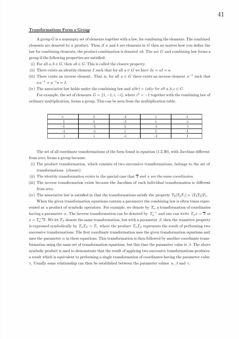
8/6/2019 Introduction to Tensor Calculus Continuum Mechanics - J. Heinbockel
http://slidepdf.com/reader/full/introduction-to-tensor-calculus-continuum-mechanics-j-heinbockel 45/372
41
Transformations Form a Group
A group G is a nonempty set of elements together with a law, for combining the elements. The combined
elements are denoted by a product. Thus, if a and b are elements in G then no matter how you define the
law for combining elements, the product combination is denoted ab. The set G and combining law forms a
group if the following properties are satisfied:(i) For all a, b ∈ G, then ab ∈ G. This is called the closure property.
(ii) There exists an identity element I such that for all a ∈ G we have Ia = aI = a.
(iii) There exists an inverse element. That is, for all a ∈ G there exists an inverse element a−1 such that
a a−1 = a−1a = I.
(iv) The associative law holds under the combining law and a(bc) = (ab)c for all a,b,c ∈ G.
For example, the set of elements G = 1,−1, i,−i, where i2 = −1 together with the combining law of
ordinary multiplication, forms a group. This can be seen from the multiplication table.
× 1 -1 i -i1 1 -1 i -i-1 -1 1 -i i-i -i i 1 -1i i -i -1 1
The set of all coordinate transformations of the form found in equation (1.2.30), with Jacobian different
from zero, forms a group because:
(i) The product transformation, which consists of two successive transformations, belongs to the set of
transformations. (closure)
(ii) The identity transformation exists in the special case that x and x are the same coordinates.(iii) The inverse transformation exists because the Jacobian of each individual transformation is different
from zero.
(iv) The associative law is satisfied in that the transformations satisfy the property T 3(T 2T 1) = (T 3T 2)T 1.
When the given transformation equations contain a parameter the combining law is often times repre-
sented as a product of symbolic operators. For example, we denote by T α a transformation of coordinates
having a parameter α. The inverse transformation can be denoted by T −1α and one can write T αx = x or
x = T −1α x. We let T β denote the same transformation, but with a parameter β , then the transitive property
is expressed symbolically by T αT β = T γ where the product T αT β represents the result of performing two
successive transformations. The first coordinate transformation uses the given transformation equations and
uses the parameter α in these equations. This transformation is then followed by another coordinate trans-
formation using the same set of transformation equations, but this time the parameter value is β. The above
symbolic product is used to demonstrate that the result of applying two successive transformations produces
a result which is equivalent to performing a single transformation of coordinates having the parameter value
γ. Usually some relationship can then be established between the parameter values α, β and γ.

8/6/2019 Introduction to Tensor Calculus Continuum Mechanics - J. Heinbockel
http://slidepdf.com/reader/full/introduction-to-tensor-calculus-continuum-mechanics-j-heinbockel 46/372
42
Figure 1.2-2. Cylindrical coordinates.
In this symbolic notation, we let T θ denote the identity transformation. That is, using the parameter
value of θ in the given set of transformation equations produces the identity transformation. The inverse
transformation can then be expressed in the form of finding the parameter value β such that T αT β = T θ.
Cartesian Coordinates
At times it is convenient to introduce an orthogonal Cartesian coordinate system having coordinates
yi, i = 1, 2, . . . , N . This space is denoted E N and represents an N-dimensional Euclidean space. Whenever
the generalized independent coordinates xi, i = 1, . . . , N are functions of the ys, and these equations are
functionally independent, then there exists independent transformation equations
yi = yi(x1, x2, . . . , xN ), i = 1, 2, . . . , N , (1.2.34)
with Jacobian different from zero. Similarly, if there is some other set of generalized coordinates, say a barred
system xi
, i = 1, . . . , N where the x
s are independent functions of the y
s, then there will exist another setof independent transformation equations
yi = yi(x1, x2, . . . , xN ), i = 1, 2, . . . , N , (1.2.35)
with Jacobian different from zero. The transformations found in the equations (1.2.34) and (1.2.35) imply
that there exists relations between the xs and xs of the form (1.2.30) with inverse transformations of the
form (1.2.32). It should be remembered that the concepts and ideas developed in this section can be applied
to a space V N of any finite dimension. Two dimensional surfaces (N = 2) and three dimensional spaces
(N = 3) will occupy most of our applications. In relativity, one must consider spaces where N = 4.
EXAMPLE 1.2-1. (cylindrical coordinates (r,θ,z)) Consider the transformation
x = x(r,θ,z) = r cos θ y = y(r,θ,z) = r sin θ z = z(r,θ,z) = z
from rectangular coordinates (x, y, z) to cylindrical coordinates (r,θ,z), illustrated in the figure 1.2-2. By
letting
y1 = x, y2 = y, y3 = z x1 = r, x2 = θ, x3 = z
the above set of equations are examples of the transformation equations (1.2.8) with u = r, v = θ, w = z as
the generalized coordinates.
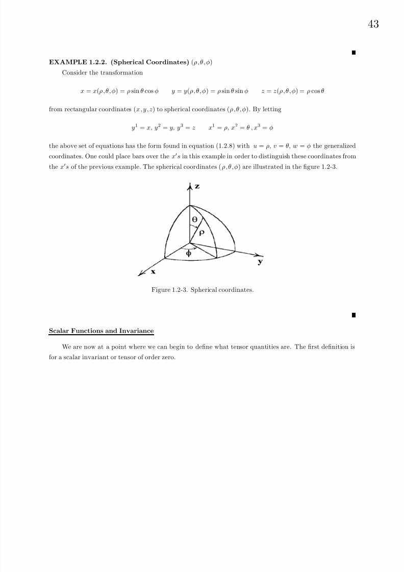
8/6/2019 Introduction to Tensor Calculus Continuum Mechanics - J. Heinbockel
http://slidepdf.com/reader/full/introduction-to-tensor-calculus-continuum-mechanics-j-heinbockel 47/372
43
EXAMPLE 1.2.2. (Spherical Coordinates) (ρ,θ,φ)
Consider the transformation
x = x(ρ,θ,φ) = ρ sin θ cos φ y = y(ρ,θ,φ) = ρ sin θ sin φ z = z(ρ,θ,φ) = ρ cos θ
from rectangular coordinates (x, y, z) to spherical coordinates (ρ,θ,φ). By letting
y1 = x, y2 = y, y3 = z x1 = ρ, x2 = θ , x3 = φ
the above set of equations has the form found in equation (1.2.8) with u = ρ, v = θ, w = φ the generalized
coordinates. One could place bars over the xs in this example in order to distinguish these coordinates from
the xs of the previous example. The spherical coordinates (ρ,θ,φ) are illustrated in the figure 1.2-3.
Figure 1.2-3. Spherical coordinates.
Scalar Functions and Invariance
We are now at a point where we can begin to define what tensor quantities are. The first definition is
for a scalar invariant or tensor of order zero.

8/6/2019 Introduction to Tensor Calculus Continuum Mechanics - J. Heinbockel
http://slidepdf.com/reader/full/introduction-to-tensor-calculus-continuum-mechanics-j-heinbockel 48/372
44
Definition: ( Absolute scalar field) Assume there exists a coordinate
transformation of the type (1.2.30) with Jacobian J different from zero. Let
the scalar function
f = f (x1, x2, . . . , xN ) (1.2.36)
be a function of the coordinates xi, i = 1, . . . , N in a space V N . Whenever
there exists a function
f = f (x1, x2, . . . , xN ) (1.2.37)
which is a function of the coordinates xi, i = 1, . . . , N such that f = J W f,
then f is called a tensor of rank or order zero of weight W in the space V N .
Whenever W = 0, the scalar f is called the component of an absolute scalar
field and is referred to as an absolute tensor of rank or order zero.
That is, an absolute scalar field is an invariant object in the space V N with respect to the group of
coordinate transformations. It has a single component in each coordinate system. For any scalar function
of the type defined by equation (1.2.36), we can substitute the transformation equations (1.2.30) and obtain
f = f (x1, . . . , xN ) = f (x1(x), . . . , xN (x)) = f (x1, . . . , xN ). (1.2.38)
Vector Transformation, Contravariant Components
In V N consider a curve C defined by the set of parametric equations
C : xi
= xi
(t), i = 1, . . . , N
where t is a parameter. The tangent vector to the curve C is the vector
T =
dx1
dt,
dx2
dt, . . . ,
dxN
dt
.
In index notation, which focuses attention on the components, this tangent vector is denoted
T i =dxi
dt, i = 1, . . . , N .
For a coordinate transformation of the type defined by equation (1.2.30) with its inverse transformation
defined by equation (1.2.32), the curve C is represented in the barred space by
xi = xi(x1(t), x2(t), . . . , xN (t)) = xi(t), i = 1, . . . , N ,
with t unchanged. The tangent to the curve in the barred system of coordinates is represented by
dxi
dt=
∂ xi
∂xj
dxj
dt, i = 1, . . . , N . (1.2.39)

8/6/2019 Introduction to Tensor Calculus Continuum Mechanics - J. Heinbockel
http://slidepdf.com/reader/full/introduction-to-tensor-calculus-continuum-mechanics-j-heinbockel 49/372
45
Letting T i, i = 1, . . . , N denote the components of this tangent vector in the barred system of coordinates,
the equation (1.2.39) can then be expressed in the form
T i
=∂xi
∂xjT j, i, j = 1, . . . , N . (1.2.40)
This equation is said to define the transformation law associated with an absolute contravariant tensor of
rank or order one. In the case N = 3 the matrix form of this transformation is representedT 1
T 2
T 3
=
∂x1
∂x1
∂x1
∂x2
∂x1
∂x3
∂x2
∂x1
∂x2
∂x2
∂x2
∂x3
∂x3
∂x1
∂x3
∂x2
∂x3
∂x3
T 1
T 2
T 3
(1.2.41)
A more general definition is
Definition: (Contravariant tensor) Whenever N quantities Ai in
a coordinate system (x1
, . . . , xN
) are related to N quantities A
i
in acoordinate system (x1, . . . , xN ) such that the Jacobian J is different
from zero, then if the transformation law
Ai
= J W ∂xi
∂xjAj
is satisfied, these quantities are called the components of a relative tensor
of rank or order one with weight W . Whenever W = 0 these quantities
are called the components of an absolute tensor of rank or order one.
We see that the above transformation law satisfies the group properties.
EXAMPLE 1.2-3. (Transitive Property of Contravariant Transformation)
Show that successive contravariant transformations is also a contravariant transformation.
Solution: Consider the transformation of a vector from an unbarred to a barred system of coordinates. A
vector or absolute tensor of rank one Ai = Ai(x), i = 1, . . . , N will transform like the equation (1.2.40) and
Ai(x) =
∂xi
∂xjAj (x). (1.2.42)
Another transformation from x → x coordinates will produce the components
Ai(x) =
∂xi
∂xj Aj
(x) (1.2.43)
Here we have used the notation Aj (x) to emphasize the dependence of the components Aj upon the x
coordinates. Changing indices and substituting equation (1.2.42) into (1.2.43) we find
Ai(x) =
∂xi
∂xj
∂xj
∂xmAm(x). (1.2.44)

8/6/2019 Introduction to Tensor Calculus Continuum Mechanics - J. Heinbockel
http://slidepdf.com/reader/full/introduction-to-tensor-calculus-continuum-mechanics-j-heinbockel 50/372
46
From the fact that∂x
i
∂xj
∂xj
∂xm=
∂xi
∂xm,
the equation (1.2.44) simplifies to
Ai(x) =
∂xi
∂x
mAm(x) (1.2.45)
and hence this transformation is also contravariant. We express this by saying that the above are transitive
with respect to the group of coordinate transformations.
Note that from the chain rule one can write
∂xm
∂xj
∂xj
∂xn=
∂xm
∂x1
∂x1
∂xn+
∂xm
∂x2
∂x2
∂xn+
∂xm
∂x3
∂x3
∂xn=
∂xm
∂xn= δm
n .
Do not make the mistake of writing
∂xm
∂x2
∂x2
∂xn=
∂xm
∂xnor
∂xm
∂x3
∂x3
∂xn=
∂xm
∂xn
as these expressions are incorrect. Note that there are no summations in these terms, whereas there is a
summation index in the representation of the chain rule.
Vector Transformation, Covariant Components
Consider a scalar invariant A(x) = A(x) which is a shorthand notation for the equation
A(x1, x2, . . . , xn) = A(x1, x2, . . . , xn)
involving the coordinate transformation of equation (1.2.30). By the chain rule we differentiate this invariant
and find that the components of the gradient must satisfy
∂A
∂xi =∂A
∂xj
∂xj
∂xi . (1.2.46)
Let
Aj =∂A
∂xjand Ai =
∂A
∂xi,
then equation (1.2.46) can be expressed as the transformation law
Ai = Aj∂xj
∂xi . (1.2.47)
This is the transformation law for an absolute covariant tensor of rank or order one. A more general definition
is
8/6/2019 Introduction to Tensor Calculus Continuum Mechanics - J. Heinbockel
http://slidepdf.com/reader/full/introduction-to-tensor-calculus-continuum-mechanics-j-heinbockel 51/372
47
Definition: (Covariant tensor) Whenever N quantities Ai in a
coordinate system (x1, . . . , xN ) are related to N quantities Ai in a co-
ordinate system (x1, . . . , xN ), with Jacobian J different from zero, such
that the transformation law
Ai = J W ∂xj
∂xi Aj (1.2.48)
is satisfied, then these quantities are called the components of a relative
covariant tensor of rank or order one having a weight of W . When-
ever W = 0, these quantities are called the components of an absolute
covariant tensor of rank or order one.
Again we note that the above transformation satisfies the group properties. Absolute tensors of rank or
order one are referred to as vectors while absolute tensors of rank or order zero are referred to as scalars.EXAMPLE 1.2-4. (Transitive Property of Covariant Transformation)
Consider a sequence of transformation laws of the type defined by the equation (1.2.47)
x → x
x → x
Ai(x) = Aj (x)∂xj
∂xi
Ak(x) = Am(x)∂xm
∂xk
We can therefore express the transformation of the components associated with the coordinate transformation
x → x and
Ak(x) = Aj (x)∂xj
∂xm
∂xm
∂xk
= Aj (x)∂xj
∂xk
,
which demonstrates the transitive property of a covariant transformation.
Higher Order Tensors
We have shown that first order tensors are quantities which obey certain transformation laws. Higher
order tensors are defined in a similar manner and also satisfy the group properties. We assume that we are
given transformations of the type illustrated in equations (1.2.30) and (1.2.32) which are single valued and
continuous with Jacobian J different from zero. Further, the quantities xi and xi, i = 1, . . . , n represent the
coordinates in any two coordinate systems. The following transformation laws define second order and third
order tensors.
8/6/2019 Introduction to Tensor Calculus Continuum Mechanics - J. Heinbockel
http://slidepdf.com/reader/full/introduction-to-tensor-calculus-continuum-mechanics-j-heinbockel 52/372

8/6/2019 Introduction to Tensor Calculus Continuum Mechanics - J. Heinbockel
http://slidepdf.com/reader/full/introduction-to-tensor-calculus-continuum-mechanics-j-heinbockel 53/372
49
General Definition
In general a mixed tensor of rank or order (m + n)
T i1i2...imj1j2...jn (1.2.53)
is contravariant of order m and covariant of order n if it obeys the transformation law
T i1i2...imj1j2...jn =
J x
x
W
T a1a2...amb1b2...bn
∂xi1
∂xa1
∂xi2
∂xa2· · · ∂xim
∂xam· ∂xb1
∂xj1
∂xb2
∂xj2· · · ∂xbn
∂xjn(1.2.54)
where
J x
x
=
∂x
∂x
=∂ (x1, x2, . . . , xN )
∂ (x1, x2, . . . , xN )
is the Jacobian of the transformation. When W = 0 the tensor is called an absolute tensor, otherwise it is
called a relative tensor of weight W.
Here superscripts are used to denote contravariant components and subscripts are used to denote covari-
ant components. Thus, if we are given the tensor components in one coordinate system, then the componentsin any other coordinate system are determined by the transformation law of equation (1.2.54). Throughout
the remainder of this text one should treat all tensors as absolute tensors unless specified otherwise.
Dyads and Polyads
Note that vectors can be represented in bold face type with the notation
A = AiEi
This notation can also be generalized to tensor quantities. Higher order tensors can also be denoted by bold
face type. For example the tensor components T ij and Bijk can be represented in terms of the basis vectors
Ei, i = 1, . . . , N by using a notation which is similar to that for the representation of vectors. For example,
T = T ijEiEj
B = Bijk EiEjEk.
Here T denotes a tensor with components T ij and B denotes a tensor with components Bijk . The quantities
EiEj are called unit dyads and EiEjEk are called unit triads. There is no multiplication sign between the
basis vectors. This notation is called a polyad notation. A further generalization of this notation is the
representation of an arbitrary tensor using the basis and reciprocal basis vectors in bold type. For example,
a mixed tensor would have the polyadic representation
T = T ij...klm...nEiEj . . . EkElEm . . . En.
A dyadic is formed by the outer or direct product of two vectors. For example, the outer product of the
vectors
a = a1E1 + a2E2 + a3E3 and b = b1E1 + b2E2 + b3E3

8/6/2019 Introduction to Tensor Calculus Continuum Mechanics - J. Heinbockel
http://slidepdf.com/reader/full/introduction-to-tensor-calculus-continuum-mechanics-j-heinbockel 54/372
50
gives the dyadab =a1b1E1E1 + a1b2E1E2 + a1b3E1E3
a2b1E2E1 + a2b2E2E2 + a2b3E2E3
a3b1E3E1 + a3b2E3E2 + a3b3E3E3.
In general, a dyad can be represented
A = AijEiEj i, j = 1, . . . , N
where the summation convention is in effect for the repeated indices. The coefficients Aij are called the
coefficients of the dyad. When the coefficients are written as an N × N array it is called a matrix. Every
second order tensor can be written as a linear combination of dyads. The dyads form a basis for the second
order tensors. As the example above illustrates, the nine dyads E1E1 , E1E2, . . . , E3E3 , associated with
the outer products of three dimensional base vectors, constitute a basis for the second order tensor A = ab
having the components Aij = aibj with i, j = 1, 2, 3. Similarly, a triad has the form
T = T ijk EiEj Ek Sum on repeated indices
where i,j,k have the range 1, 2, . . . , N . The set of outer or direct products EiEjEk , with i,j,k = 1, . . . , N
constitutes a basis for all third order tensors. Tensor components with mixed suffixes like C ijk are associated
with triad basis of the form
C = C ijk EiEj Ek
where i,j,k have the range 1, 2, . . . N . Dyads are associated with the outer product of two vectors, while triads,
tetrads,... are associated with higher-order outer products. These higher-order outer or direct products are
referred to as polyads.
The polyad notation is a generalization of the vector notation. The subject of how polyad componentstransform between coordinate systems is the subject of tensor calculus.
In Cartesian coordinates we have Ei = Ei = ei and a dyadic with components called dyads is written
A = Aij ei ej orA =A11 e1 e1 + A12 e1 e2 + A13 e1 e3
A21 e2 e1 + A22 e2 e2 + A23 e2 e3
A31 e3 e1 + A32 e3 e2 + A33 e3 e3
where the terms
ei
ej are called unit dyads. Note that a dyadic has nine components as compared with a
vector which has only three components. The conjugate dyadic Ac is defined by a transposition of the unit
vectors in A, to obtainAc =A11 e1 e1 + A12 e2 e1 + A13 e3 e1
A21 e1 e2 + A22 e2 e2 + A23 e3 e2
A31 e1 e3 + A32 e2 e3 + A33 e3 e3
8/6/2019 Introduction to Tensor Calculus Continuum Mechanics - J. Heinbockel
http://slidepdf.com/reader/full/introduction-to-tensor-calculus-continuum-mechanics-j-heinbockel 55/372
51
If a dyadic equals its conjugate A = Ac, then Aij = Aji and the dyadic is called symmetric. If a dyadic
equals the negative of its conjugate A = −Ac, then Aij = −Aji and the dyadic is called skew-symmetric. A
special dyadic called the identical dyadic or idemfactor is defined by
J =
e1
e1 +
e2
e2 +
e3
e3.
This dyadic has the property that pre or post dot product multiplication of J with a vector V produces the
same vector V . For example,
V · J = (V 1 e1 + V 2 e2 + V 3 e3) · J
= V 1 e1 · e1 e1 + V 2 e2 · e2 e2 + V 3 e3 · e3 e3 = V
and J · V = J · (V 1 e1 + V 2 e2 + V 3 e3)
= V 1 e1 e1 · e1 + V 2 e2 e2 · e2 + V 3 e3 e3 · e3 = V
A dyadic operation often used in physics and chemistry is the double dot product A : B where A and
B are both dyadics. Here both dyadics are expanded using the distributive law of multiplication, and then
each unit dyad pair
ei
ej :
em
en are combined according to the rule
ei ej : em en = ( ei · em)( ej · en).For example, if A = Aij ei ej and B = Bij ei ej, then the double dot product A : B is calculated as follows.
A : B = (Aij ei ej ) : (Bmn em en) = Aij Bmn( ei ej : em en) = Aij Bmn( ei · em)( ej · en)
= Aij Bmnδimδjn = AmjBmj
= A11B11 + A12B12 + A13B13
+ A21B21 + A22B22 + A23B23
+ A31B31 + A32B32 + A33B33
When operating with dyads, triads and polyads, there is a definite order to the way vectors and polyad
components are represented. For example, for A = Ai ei and B = Bi
ei vectors with outer product
A B = AmBn em en = φ
there is produced the dyadic φ with components AmBn. In comparison, the outer product
B A = BmAn em en = ψ
produces the dyadic ψ with components BmAn. That is
φ = A B =A1B1 e1 e1 + A1B2 e1 e2 + A1B3 e1 e3
A2B1 e2 e1 + A2B2 e2 e2 + A2B3 e2 e3
A3B1 e3 e1 + A3B2 e3 e2 + A3B3 e3 e3
and ψ = B A =B1A1
e1
e1 + B1A2
e1
e2 + B1A3
e1
e3
B2A1 e2 e1 + B2A2 e2 e2 + B2A3 e2 e3
B3A1 e3 e1 + B3A2 e3 e2 + B3A3 e3 e3
are different dyadics.
The scalar dot product of a dyad with a vector C is defined for both pre and post multiplication as
φ · C = A B · C = A( B · C )
C · φ = C · A B =( C · A) B
These products are, in general, not equal.

8/6/2019 Introduction to Tensor Calculus Continuum Mechanics - J. Heinbockel
http://slidepdf.com/reader/full/introduction-to-tensor-calculus-continuum-mechanics-j-heinbockel 56/372
52
Operations Using Tensors
The following are some important tensor operations which are used to derive special equations and to
prove various identities.
Addition and Subtraction
Tensors of the same type and weight can be added or subtracted. For example, two third order mixed
tensors, when added, produce another third order mixed tensor. Let Aijk and Bi
jk denote two third order
mixed tensors. Their sum is denoted
C ijk = Aijk + Bi
jk.
That is, like components are added. The sum is also a mixed tensor as we now verify. By hypothesis Aijk
and Bijk are third order mixed tensors and hence must obey the transformation laws
Aijk = Am
np
∂xi
∂xm
∂xn
∂xj
∂x p
∂xk
Bi
jk = Bmnp
∂xi
∂xm
∂xn
∂xj
∂x p
∂xk.
We let C ijk = Aijk + Bi
jk denote the sum in the transformed coordinates. Then the addition of the above
transformation equations produces
C i
jk =
Ai
jk + Bi
jk
=
Amnp + Bm
np
∂xi
∂xm
∂xn
∂xj
∂x p
∂xk= C mnp
∂xi
∂xm
∂xn
∂xj
∂x p
∂xk.
Consequently, the sum transforms as a mixed third order tensor.
Multiplication (Outer Product)
The product of two tensors is also a tensor. The rank or order of the resulting tensor is the sum of
the ranks of the tensors occurring in the multiplication. As an example, let Aijk denote a mixed third order
tensor and let Blm denote a mixed second order tensor. The outer product of these two tensors is the fifth
order tensor
C iljkm = Ai
jk Blm, i,j,k,l,m = 1, 2, . . . , N .
Here all indices are free indices as i, j, k, l , m take on any of the integer values 1, 2, . . . , N . Let Ai
jk and Bl
m
denote the components of the given tensors in the barred system of coordinates. We define C iljkm as the
outer product of these components. Observe that C iljkm is a tensor for by hypothesis Ai
jk and Blm are tensors
and hence obey the transformation laws
Aαβγ = Ai
jk
∂xα
∂xi
∂xj
∂xβ
∂xk
∂xγ
Bδ = Bl
m
∂xδ
∂xl
∂xm
∂x .
(1.2.55)
The outer product of these components produces
C αδβγ = A
αβγ B
δ = Ai
jk Blm
∂xα
∂xi
∂xj
∂xβ
∂xk
∂xγ
∂xδ
∂xl
∂xm
∂x
= C iljkm
∂xα
∂xi
∂xj
∂xβ
∂xk
∂xγ
∂xδ
∂xl
∂xm
∂x
(1.2.56)
which demonstrates that C iljkm transforms as a mixed fifth order absolute tensor. Other outer products are
analyzed in a similar way.

8/6/2019 Introduction to Tensor Calculus Continuum Mechanics - J. Heinbockel
http://slidepdf.com/reader/full/introduction-to-tensor-calculus-continuum-mechanics-j-heinbockel 57/372
53
Contraction
The operation of contraction on any mixed tensor of rank m is performed when an upper index is
set equal to a lower index and the summation convention is invoked. When the summation is performed
over the repeated indices the resulting quantity is also a tensor of rank or order (m − 2). For example, let
Ai
jk, i, j, k = 1, 2, . . . , N denote a mixed tensor and perform a contraction by setting j equal to i. We obtain
Aiik = A1
1k + A22k + · · · + AN
Nk = Ak (1.2.57)
where k is a free index. To show that Ak is a tensor, we let Aiik = Ak denote the contraction on the
transformed components of Aijk . By hypothesis Ai
jk is a mixed tensor and hence the components must
satisfy the transformation law
Aijk = Am
np
∂xi
∂xm
∂xn
∂xj
∂x p
∂xk.
Now execute a contraction by setting j equal to i and perform a summation over the repeated index. We
find
Aiik = Ak = Am
np
∂xi
∂xm
∂xn
∂xi
∂x p
∂xk= Am
np
∂xn
∂xm
∂x p
∂xk
= Amnpδn
m∂x p
∂xk= An
np∂x p
∂xk= A p
∂x p
∂xk.
(1.2.58)
Hence, the contraction produces a tensor of rank two less than the original tensor. Contractions on other
mixed tensors can be analyzed in a similar manner.
New tensors can be constructed from old tensors by performing a contraction on an upper and lower
index. This process can be repeated as long as there is an upper and lower index upon which to perform the
contraction. Each time a contraction is performed the rank of the resulting tensor is two less than the rank
of the original tensor.
Multiplication (Inner Product)
The inner product of two tensors is obtained by:
(i) first taking the outer product of the given tensors and
(ii) performing a contraction on two of the indices.
EXAMPLE 1.2-5. (Inner product)
Let Ai and Bj denote the components of two first order tensors (vectors). The outer product of these
tensors is
C ij = AiBj , i, j = 1, 2, . . . , N .
The inner product of these tensors is the scalar
C = Ai
Bi = A1
B1 + A2
B2 + · · · + AN
BN .Note that in some situations the inner product is performed by employing only subscript indices. For
example, the above inner product is sometimes expressed as
C = AiBi = A1B1 + A2B2 + · · ·AN BN .
This notation is discussed later when Cartesian tensors are considered.
8/6/2019 Introduction to Tensor Calculus Continuum Mechanics - J. Heinbockel
http://slidepdf.com/reader/full/introduction-to-tensor-calculus-continuum-mechanics-j-heinbockel 58/372
54
Quotient Law
Assume Bqsr and C s p are arbitrary absolute tensors. Further assume we have a quantity A(ijk ) which
we think might be a third order mixed tensor Aijk . By showing that the equation
ArqpBqs
r = C s p
is satisfied, then it follows that Arqp must be a tensor. This is an example of the quotient law. Obviously,
this result can be generalized to apply to tensors of any order or rank. To prove the above assertion we shall
show from the above equation that Aijk is a tensor. Let xi and xi denote a barred and unbarred system of
coordinates which are related by transformations of the form defined by equation (1.2.30). In the barred
system, we assume that
ArqpB
qsr = C
s p (1.2.59)
where by hypothesis Bijk and C lm are arbitrary absolute tensors and therefore must satisfy the transformation
equations
Bqs
r= Bij
k
∂xq
∂xi
∂xs
∂xj
∂xk
∂xr
C s
p = C lm∂xs
∂xl
∂xm
∂x p .
We substitute for Bqsr and C
s p in the equation (1.2.59) and obtain the equation
Arqp
Bij
k
∂xq
∂xi
∂xs
∂xj
∂xk
∂xr
=
C lm
∂xs
∂xl
∂xm
∂x p
= Ar
qmBqlr
∂xs
∂xl
∂xm
∂x p .
Since the summation indices are dummy indices they can be replaced by other symbols. We change l to j,
q to i and r to k and write the above equation as
∂xs
∂xjA
rqp
∂xq
∂xi∂xk
∂xr − Akim
∂xm
∂x pBij
k = 0.
Use inner multiplication by ∂xn
∂xs and simplify this equation to the form
δnj
A
rqp
∂xq
∂xi
∂xk
∂xr − Akim
∂xm
∂x p
Bij
k = 0 orA
rqp
∂xq
∂xi
∂xk
∂xr − Akim
∂xm
∂x p
Bin
k = 0.
Because Bink is an arbitrary tensor, the quantity inside the brackets is zero and therefore
Ar
qp
∂xq
∂xi
∂xk
∂xr −Ak
im
∂xm
∂x p= 0.
This equation is simplified by inner multiplication by ∂xi
∂xj∂xl
∂xk to obtain
δqj δl
rAr
qp − Akim
∂xm
∂x p
∂xi
∂xj
∂xl
∂xk= 0 or
Aljp = Ak
im
∂xm
∂x p
∂xi
∂xj
∂xl
∂xk
which is the transformation law for a third order mixed tensor.

8/6/2019 Introduction to Tensor Calculus Continuum Mechanics - J. Heinbockel
http://slidepdf.com/reader/full/introduction-to-tensor-calculus-continuum-mechanics-j-heinbockel 59/372
55
EXERCISE 1.2
1. Consider the transformation equations representing a rotation of axes through an angle α.
T α : x1 = x1 cos α − x2 sin α
x2 = x1 sin α + x2 cos α
Treat α as a parameter and show this set of transformations constitutes a group by finding the value of α
which:
(i) gives the identity transformation.
(ii) gives the inverse transformation.
(iii) show the transformation is transitive in that a transformation with α = θ1 followed by a transformation
with α = θ2 is equivalent to the transformation using α = θ1 + θ2.
2. Show the transformation
T α :
x1 = αx1
x2 = 1α
x2
forms a group with α as a parameter. Find the value of α such that:(i) the identity transformation exists.
(ii) the inverse transformation exists.
(iii) the transitive property is satisfied.
3. Show the given transformation forms a group with parameter α.
T α :
x1 = x1
1−αx1
x2 = x2
1−αx1
4. Consider the Lorentz transformation from relativity theory having the velocity parameter V, c is the
speed of light and x4 = t is time.
T V :
x1 = x1
−V x4
1−V 2
c2
x2 = x2
x3 = x3
x4 =x4−V x1
c2 1−V 2
c2
Show this set of transformations constitutes a group, by establishing:
(i) V = 0 gives the identity transformation T 0.
(ii) T V 2 · T V 1 = T 0 requires that V 2 = −V 1.
(iii) T V 2 · T V 1 = T V 3 requires that
V 3 =
V 1 + V 2
1 + V 1V 2c2 .
5. For ( E 1, E 2, E 3) an arbitrary independent basis, (a) Verify that
E 1 =1
V E 2 × E 3, E 2 =
1
V E 3 × E 1, E 3 =
1
V E 1 × E 2
is a reciprocal basis, where V = E 1 · ( E 2 × E 3) (b) Show that E j = gij E i.

8/6/2019 Introduction to Tensor Calculus Continuum Mechanics - J. Heinbockel
http://slidepdf.com/reader/full/introduction-to-tensor-calculus-continuum-mechanics-j-heinbockel 60/372
56
Figure 1.2-4. Cylindrical coordinates (r,β,z).
6. For the cylindrical coordinates (r,β,z) illustrated in the figure 1.2-4.
(a) Write out the transformation equations from rectangular (x, y, z) coordinates to cylindrical (r,β,z)
coordinates. Also write out the inverse transformation.
(b) Determine the following basis vectors in cylindrical coordinates and represent your results in terms of
cylindrical coordinates.
(i) The tangential basis E 1, E 2, E 3. (ii)The normal basis E 1, E 2, E 3. (iii) er, eβ , ez
where er, eβ, ez are normalized vectors in the directions of the tangential basis.
(c) A vector A = Ax
e1 + Ay
e2 + Az
e3 can be represented in any of the forms:
A = A1 E 1 + A2 E 2 + A3 E 3
A = A1 E 1 + A2
E 2 + A3 E 3
A = Arer + Aβ eβ + Azez
depending upon the basis vectors selected . In terms of the components Ax, Ay, Az
(i) Solve for the contravariant components A1, A2, A3.
(ii) Solve for the covariant components A1, A2, A3.
(iii) Solve for the components Ar, Aβ , Az. Express all results in cylindrical coordinates. (Note the
components Ar, Aβ , Az are referred to as physical components. Physical components are considered in
more detail in a later section.)
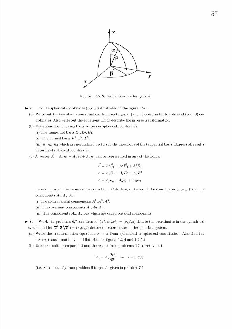
8/6/2019 Introduction to Tensor Calculus Continuum Mechanics - J. Heinbockel
http://slidepdf.com/reader/full/introduction-to-tensor-calculus-continuum-mechanics-j-heinbockel 61/372
57
Figure 1.2-5. Spherical coordinates (ρ,α,β ).
7. For the spherical coordinates (ρ,α,β ) illustrated in the figure 1.2-5.
(a) Write out the transformation equations from rectangular (x, y, z) coordinates to spherical (ρ,α,β ) co-ordinates. Also write out the equations which describe the inverse transformation.
(b) Determine the following basis vectors in spherical coordinates
(i) The tangential basis E 1, E 2, E 3.
(ii) The normal basis E 1, E 2, E 3.
(iii) eρ, eα, eβ which are normalized vectors in the directions of the tangential basis. Express all results
in terms of spherical coordinates.
(c) A vector A = Ax e1 + Ay e2 + Az e3 can be represented in any of the forms:
A = A1 E 1 + A2 E 2 + A3 E 3
A = A1 E 1 + A2 E 2 + A3 E 3
A = Aρeρ + Aαeα + Aβ eβ
depending upon the basis vectors selected . Calculate, in terms of the coordinates (ρ,α,β ) and the
components Ax, Ay, Az
(i) The contravariant components A1, A2, A3.
(ii) The covariant components A1, A2, A3.
(iii) The components Aρ, Aα, Aβ which are called physical components.
8. Work the problems 6,7 and then let (x1, x2, x3) = (r,β,z) denote the coordinates in the cylindrical
system and let (x1, x2, x3) = (ρ,α,β ) denote the coordinates in the spherical system.
(a) Write the transformation equations x → x from cylindrical to spherical coordinates. Also find the
inverse transformations. ( Hint: See the figures 1.2-4 and 1.2-5.)
(b) Use the results from part (a) and the results from problems 6,7 to verify that
Ai = Aj∂xj
∂xi for i = 1, 2, 3.
(i.e. Substitute Aj from problem 6 to get Ai given in problem 7.)
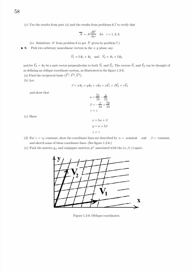
8/6/2019 Introduction to Tensor Calculus Continuum Mechanics - J. Heinbockel
http://slidepdf.com/reader/full/introduction-to-tensor-calculus-continuum-mechanics-j-heinbockel 62/372
58
(c) Use the results from part (a) and the results from problems 6,7 to verify that
Ai
= Aj ∂xi
∂xjfor i = 1, 2, 3.
(i.e. Substitute Aj from problem 6 to get Ai given by problem 7.)
9. Pick two arbitrary noncolinear vectors in the x, y plane, say
V 1 = 5 e1 + e2 and V 2 = e1 + 5 e2
and let V 3 = e3 be a unit vector perpendicular to both V 1 and V 2. The vectors V 1 and V 2 can be thought of
as defining an oblique coordinate system, as illustrated in the figure 1.2-6.
(a) Find the reciprocal basis ( V 1, V 2, V 3).
(b) Let
r = x e1 + y e2 + z e3 = α V 1 + β V 2 + γ V 3
and show that
α = 5x24
− y24
β = − x
24+
5y
24γ = z
(c) Showx = 5α + β
y = α + 5β
z = γ
(d) For γ = γ 0 constant, show the coordinate lines are described by α = constant and β = constant,
and sketch some of these coordinate lines. (See figure 1.2-6.)(e) Find the metrics gij and conjugate metrices gij associated with the (α, β, γ ) space.
Figure 1.2-6. Oblique coordinates.

8/6/2019 Introduction to Tensor Calculus Continuum Mechanics - J. Heinbockel
http://slidepdf.com/reader/full/introduction-to-tensor-calculus-continuum-mechanics-j-heinbockel 63/372
59
10. Consider the transformation equations
x = x(u, v, w)
y = y(u, v, w)
z = z(u, v, w)
substituted into the position vector
r = x e1 + y e2 + z e3.
Define the basis vectors
( E 1, E 2, E 3) =
∂r
∂u,
∂r
∂v,
∂r
∂w
with the reciprocal basis
E 1 =1
V E 2 × E 3, E 2 =
1
V E 3 × E 1, E 3 =
1
V E 1 × E 2.
where
V = E 1 · ( E 2 × E 3).
Let v = E 1 · ( E 2 × E 3) and show that v · V = 1.
11. Given the coordinate transformation
x = −u − 2v y = −u − v z = z
(a) Find and illustrate graphically some of the coordinate curves.
(b) For r = r(u, v, z) a position vector, define the basis vectors
E 1 =
∂r
∂u , E 2 =
∂r
∂v , E 3 =
∂r
∂z .
Calculate these vectors and then calculate the reciprocal basis E 1, E 2, E 3.
(c) With respect to the basis vectors in (b) find the contravariant components Ai associated with the vector
A = α1 e1 + α2 e2 + α3 e3
where (α1, α2, α3) are constants.
(d) Find the covariant components Ai associated with the vector A given in part (c).
(e) Calculate the metric tensor gij and conjugate metric tensor gij .
(f) From the results (e), verify that gijgjk = δki
(g) Use the results from (c)(d) and (e) to verify that Ai = gikAk
(h) Use the results from (c)(d) and (e) to verify that Ai = gikAk
(i) Find the projection of the vector A on unit vectors in the directions E 1, E 2, E 3.
(j) Find the projection of the vector A on unit vectors the directions E 1, E 2, E 3.
8/6/2019 Introduction to Tensor Calculus Continuum Mechanics - J. Heinbockel
http://slidepdf.com/reader/full/introduction-to-tensor-calculus-continuum-mechanics-j-heinbockel 64/372
60
12. For r = yi ei where yi = yi(x1, x2, x3), i = 1, 2, 3 we have by definition
E j =∂r
∂xj=
∂y i
∂xjei. From this relation show that E m =
∂xm
∂y jej
and consequently
gij = E i · E j =∂y m
∂xi
∂y m
∂xj, and gij = E i · E j =
∂xi
∂y m
∂xj
∂y m, i, j, m = 1, . . . , 3
13. Consider the set of all coordinate transformations of the form
yi = aij xj + bi
where aij and bi are constants and the determinant of ai
j is different from zero. Show this set of transforma-
tions forms a group.
14. For αi , β i constants and t a parameter, xi = αi + t β i,i = 1, 2, 3 is the parametric representation of
a straight line. Find the parametric equation of the line which passes through the two points (1, 2, 3) and
(14, 7,−3). What does the vector drdt represent?
15. A surface can be represented using two parameters u, v by introducing the parametric equations
xi = xi(u, v), i = 1, 2, 3, a < u < b and c < v < d.
The parameters u, v are called the curvilinear coordinates of a point on the surface. A point on the surface
can be represented by the position vector r = r(u, v) = x1(u, v) e1 + x2(u, v) e2 + x3(u, v) e3. The vectors ∂r∂u
and ∂r∂v are tangent vectors to the coordinate surface curves r(u, c2) and r(c1, v) respectively. An element of
surface area dS on the surface is defined as the area of the elemental parallelogram having the vector sides∂r∂u du and ∂r
∂v dv. Show that
dS = | ∂r
∂u× ∂r
∂v| dudv =
g11g22 − (g12)2 dudv
where
g11 =∂r
∂u· ∂r
∂ug12 =
∂r
∂u· ∂r
∂vg22 =
∂r
∂v· ∂r
∂v.
Hint: ( A × B) · ( A × B) = | A × B|2 See Exercise 1.1, problem 9(c).
16.
(a) Use the results from problem 15 and find the element of surface area of the circular cone
x = u sin α cos v y = u sin α sin v z = u cos α
α a constant 0 ≤ u ≤ b 0 ≤ v ≤ 2π
(b) Find the surface area of the above cone.

8/6/2019 Introduction to Tensor Calculus Continuum Mechanics - J. Heinbockel
http://slidepdf.com/reader/full/introduction-to-tensor-calculus-continuum-mechanics-j-heinbockel 65/372
61
17. The equation of a plane is defined in terms of two parameters u and v and has the form
xi = αi u + β i v + γ i i = 1, 2, 3,
where αi β i and γ i are constants. Find the equation of the plane which passes through the points (1, 2, 3),
(14, 7,−3) and (5, 5, 5). What does this problem have to do with the position vector r(u, v), the vectors∂r∂u , ∂r
∂v and r(0, 0)? Hint: See problem 15.
18. Determine the points of intersection of the curve x1 = t, x2 = (t)2, x3 = (t)3 with the plane
8 x1 − 5 x2 + x3 − 4 = 0.
19. Verify the relations V eijk E k = E i × E j and v−1 eijk E k = E i × E j where v = E 1 · ( E 2 × E 3) and
V = E 1 · ( E 2 × E 3)..
20. Let xi and xi, i = 1, 2, 3 be related by the linear transformation xi = cij xj , where ci
j are constants
such that the determinant c = det(cij ) is different from zero. Let γ
nm denote the cofactor of c
mn divided by
the determinant c.
(a) Show that cij γ jk = γ ij cj
k = δik.
(b) Show the inverse transformation can be expressed xi = γ ij xj .
(c) Show that if Ai is a contravariant vector, then its transformed components are A p = c pqAq.
(d) Show that if Ai is a covariant vector, then its transformed components are Ai = γ pi A p.
21. Show that the outer product of two contravariant vectors Ai and Bi, i = 1, 2, 3 results in a second
order contravariant tensor.
22. Show that for the position vector r = yi(x1, x2, x3)
ei the element of arc length squared is
ds2 = dr · dr = gijdxidxj where gij = E i · E j = ∂ym
∂xi ∂ym
∂xj .
23. For Aijk , Bm
n and C ptq absolute tensors, show that if Aijk Bk
n = C ijn then Aijk B
kn = C
ijn.
24. Let Aij denote an absolute covariant tensor of order 2. Show that the determinant A = det(Aij ) is
an invariant of weight 2 and
(A) is an invariant of weight 1.
25. Let Bij denote an absolute contravariant tensor of order 2. Show that the determinant B = det(Bij )
is an invariant of weight −2 and√
B is an invariant of weight −1.
26.
(a) Write out the contravariant components of the following vectors
(i) E 1 (ii) E 2 (iii) E 3 where E i =∂r
∂xifor i = 1, 2, 3.
(b) Write out the covariant components of the following vectors
(i) E 1 (ii) E 2 (ii) E 3 where E i = grad xi, for i = 1, 2, 3.

8/6/2019 Introduction to Tensor Calculus Continuum Mechanics - J. Heinbockel
http://slidepdf.com/reader/full/introduction-to-tensor-calculus-continuum-mechanics-j-heinbockel 66/372

8/6/2019 Introduction to Tensor Calculus Continuum Mechanics - J. Heinbockel
http://slidepdf.com/reader/full/introduction-to-tensor-calculus-continuum-mechanics-j-heinbockel 67/372
63
40. Let Ai = Ai(x1, x2, . . . , xN ) denote the components of an absolute contravariant tensor. Form the
quantity Bij = ∂Ai
∂xj and determine if Bij transforms like a tensor.
41. Let Ai denote the components of a covariant vector. (a) Show that aij =∂Ai
∂xj− ∂Aj
∂xiare the
components of a second order tensor. (b) Show that∂aij
∂xk
+∂ajk
∂xi
+∂aki
∂xj
= 0.
42. Show that xi = K eijk Aj Bk, with K = 0 and arbitrary, is a general solution of the system of equations
Aixi = 0, Bixi = 0, i = 1, 2, 3. Give a geometric interpretation of this result in terms of vectors.
43. Given the vector A = y e1 + z e2 + x e3 where e1, e2, e3 denote a set of unit basis vectors which
define a set of orthogonal x, y, z axes. Let E 1 = 3 e1 + 4 e2, E 2 = 4 e1 + 7 e2 and E 3 = e3 denote a set of
basis vectors which define a set of u, v, w axes. (a) Find the coordinate transformation between these two
sets of axes. (b) Find a set of reciprocal vectors E 1, E 3, E 3. (c) Calculate the covariant components of A.
(d) Calculate the contravariant components of A.
44. Let A = Aij
ei
ej denote a dyadic. Show that
A : Ac = A11A11 + A12A21 + A13A31 + A21A12 + A22A22 + A23A32 + A31A13 + A32A23 + A23A33
45. Let A = Ai ei, B = Bi ei, C = C i ei, D = Di ei denote vectors and let φ = A B, ψ = C D denote
dyadics which are the outer products involving the above vectors. Show that the double dot product satisfies
φ : ψ = A B : C D = ( A · C )( B · D)
46. Show that if aij is a symmetric tensor in one coordinate system, then it is symmetric in all coordinate
systems.
47. Write the transformation laws for the given tensors. (a) Akij (b) A
ijk (c) A
ijkm
48. Show that if Ai = Aj∂xj
∂xi , then Ai = Aj∂xj
∂xi . Note that this is equivalent to interchanging the bar
and unbarred systems.
49.
(a) Show that under the linear homogeneous transformation
x1 =a11x1 + a2
1x2
x2 =a12x1 + a2
2x2
the quadratic form
Q(x1, x2) = g11(x1)2 + 2g12x1x2 + g22(x2)2 becomes Q(x1, x2) = g11(x1)2 + 2g12x1x2 + g22(x2)2
where gij = g11aj1ai
1 + g12(ai1aj
2 + aj1ai
2) + g22ai2aj
2.
(b) Show F = g11g22− (g12)2 is a relative invariant of weight 2 of the quadratic form Q(x1, x2) with respect
to the group of linear homogeneous transformations. i.e. Show that F = ∆2F where F = g11g22−(g12)2
and ∆ = (a11a2
2 − a21a1
2).
8/6/2019 Introduction to Tensor Calculus Continuum Mechanics - J. Heinbockel
http://slidepdf.com/reader/full/introduction-to-tensor-calculus-continuum-mechanics-j-heinbockel 68/372
64
50. Let ai and bi for i = 1, . . . , n denote arbitrary vectors and form the dyadic
Φ = a1b1 + a2b2 + · · · + anbn.
By definition the first scalar invariant of Φ is
φ1 = a1 · b1 + a2 · b2 + · · · + an · bn
where a dot product operator has been placed between the vectors. The first vector invariant of Φ is defined
φ = a1 × b1 + a2 × b2 + · · · + an × bn
where a vector cross product operator has been placed between the vectors.
(a) Show that the first scalar and vector invariant of
Φ = e1 e2 + e2 e3 + e3 e3
are respectively 1 and e1 + e3.
(b) From the vector f = f 1
e1 + f 2
e2 + f 3
e3 one can form the dyadic ∇f having the matrix components
∇f = ∂f 1∂x
∂f 2∂x
∂f 3∂x
∂f 1∂y
∂f 2∂y
∂f 3∂y
∂f 1∂z
∂f 2∂z
∂f 3∂z
.
Show that this dyadic has the first scalar and vector invariants given by
∇ · f =∂f 1∂x
+∂f 2∂y
+∂f 3∂z
∇× f =
∂f 3∂y
− ∂f 2∂z
e1 +
∂f 1∂z
− ∂f 3∂x
e2 +
∂f 2∂x
− ∂f 1∂y
e3
51. Let Φ denote the dyadic given in problem 50. The dyadic Φ2 defined by
Φ2 =1
2
i,j
ai × aj bi × bj
is called the Gibbs second dyadic of Φ, where the summation is taken over all permutations of i and j. Wheni = j the dyad vanishes. Note that the permutations i, j and j, i give the same dyad and so occurs twice
in the final sum. The factor 1/2 removes this doubling. Associated with the Gibbs dyad Φ2 are the scalar
invariants
φ2 =1
2
i,j
(ai × aj ) · (bi × bj )
φ3 =1
6
i,j,k
(ai × aj · ak)(bi × bj · bk)
Show that the dyad
Φ = a s + t q + c u
hasthe first scalar invariant φ1 = a · s + b · t + c · u
the first vector invariant φ = a × s + b × t + c × u
Gibbs second dyad Φ2 = b × ct× u + c × au × s + a × bs × t
second scalar of Φ φ2 = (b × c) · (t · u) + (c × a) · (u × s) + (a × b) · (s × t)
third scalar of Φ φ3 = (a × b · c)(s × t · u)
8/6/2019 Introduction to Tensor Calculus Continuum Mechanics - J. Heinbockel
http://slidepdf.com/reader/full/introduction-to-tensor-calculus-continuum-mechanics-j-heinbockel 69/372
65
52. (Spherical Trigonometry) Construct a spherical triangle ABC on the surface of a unit sphere with
sides and angles less than 180 degrees. Denote by a,b c the unit vectors from the origin of the sphere to the
vertices A,B and C. Make the construction such that a ·(b×c) is positive with a, b, c forming a right-handed
system. Let α, β, γ denote the angles between these unit vectors such that
a · b = cos γ c · a = cos β b · c = cos α. (1)
The great circles through the vertices A,B,C then make up the sides of the spherical triangle where side α
is opposite vertex A, side β is opposite vertex B and side γ is opposite the vertex C. The angles A,B and C
between the various planes formed by the vectors a, b and c are called the interior dihedral angles of the
spherical triangle. Note that the cross products
a × b = sin γ c b × c = sin α a c × a = sin β b (2)
define unit vectors a, b and c perpendicular to the planes determined by the unit vectors a, b and c. The
dot products
a·
b = cos γ b·
c = cos α c·
a = cos β (3)
define the angles α,β and γ which are called the exterior dihedral angles at the vertices A,B and C and are
such that
α = π − A β = π − B γ = π − C. (4)
(a) Using appropriate scaling, show that the vectors a, b, c and a, b, c form a reciprocal set.
(b) Show that a · (b × c) = sin α a · a = sin β b · b = sin γ c · c
(c) Show that a · (b × c) = sin α a · a = sin β b · b = sin γ c · c
(d) Using parts (b) and (c) show thatsin α
sin α=
sin β
sin β =
sin γ
sin γ
(e) Use the results from equation (4) to derive the law of sines for spherical triangles
sin α
sin A=
sin β
sin B=
sin γ
sin C
(f) Using the equations (2) show that
sin β sin γ b · c = (c × a) · (a × b) = (c · a)(a · b)− b · c
and hence show that
cos α = cos β cos γ − sin β sin γ cos α.
In a similar manner show also that
cos α = cos β cos γ − sin β sin γ cos α.
(g) Using part (f) derive the law of cosines for spherical triangles
cos α =cos β cos γ + sin β sin γ cos A
cos A = − cos B cos C + sin B sin C cos α
A cyclic permutation of the symbols produces similar results involving the other angles and sides of the
spherical triangle.

8/6/2019 Introduction to Tensor Calculus Continuum Mechanics - J. Heinbockel
http://slidepdf.com/reader/full/introduction-to-tensor-calculus-continuum-mechanics-j-heinbockel 70/372
65
§1.3 SPECIAL TENSORS
Knowing how tensors are defined and recognizing a tensor when it pops up in front of you are two
different things. Some quantities, which are tensors, frequently arise in applied problems and you should
learn to recognize these special tensors when they occur. In this section some important tensor quantities
are defined. We also consider how these special tensors can in turn be used to define other tensors.
Metric Tensor
Define yi, i = 1, . . . , N as independent coordinates in an N dimensional orthogonal Cartesian coordinate
system. The distance squared between two points yi and yi + dyi, i = 1, . . . , N is defined by the
expression
ds2 = dymdym = (dy1)2 + (dy2)2 + · · · + (dyN )2. (1.3.1)
Assume that the coordinates yi are related to a set of independent generalized coordinates xi, i = 1, . . . , N
by a set of transformation equations
yi = yi(x1, x2, . . . , xN ), i = 1, . . . , N . (1.3.2)
To emphasize that each yi depends upon the x coordinates we sometimes use the notation yi = yi(x), for
i = 1, . . . , N . The differential of each coordinate can be written as
dym =∂ym
∂xjdxj , m = 1, . . . , N , (1.3.3)
and consequently in the x-generalized coordinates the distance squared, found from the equation (1.3.1),
becomes a quadratic form. Substituting equation (1.3.3) into equation (1.3.1) we find
ds2 =∂ym
∂xi
∂ym
∂xjdxidxj = gij dxidxj (1.3.4)
where
gij =∂ym
∂xi
∂ym
∂xj, i, j = 1, . . . , N (1.3.5)
are called the metrices of the space defined by the coordinates xi, i = 1, . . . , N . Here the gij are functions of
the x coordinates and is sometimes written as gij = gij(x). Further, the metrices gij are symmetric in the
indices i and j so that gij = gji for all values of i and j over the range of the indices. If we transform to
another coordinate system, say xi, i = 1, . . . , N , then the element of arc length squared is expressed in terms
of the barred coordinates and ds2 = gij dxidxj , where gij = gij(x) is a function of the barred coordinates.
The following example demonstrates that these metrices are second order covariant tensors.

8/6/2019 Introduction to Tensor Calculus Continuum Mechanics - J. Heinbockel
http://slidepdf.com/reader/full/introduction-to-tensor-calculus-continuum-mechanics-j-heinbockel 71/372
8/6/2019 Introduction to Tensor Calculus Continuum Mechanics - J. Heinbockel
http://slidepdf.com/reader/full/introduction-to-tensor-calculus-continuum-mechanics-j-heinbockel 72/372
67
and consequently dr =∂r
∂udu +
∂r
∂vdv +
∂r
∂wdw, where
E 1 =∂r
∂u=
∂x
∂ue1 +
∂y
∂ue2 +
∂z
∂ue3
E 2 =∂r
∂v
=∂x
∂v e1 +∂y
∂v e2 +∂z
∂v e3 E 3 =
∂r
∂w=
∂x
∂we1 +
∂y
∂we2 +
∂z
∂we3.
(1.3.11)
are tangent vectors to the coordinate curves. The element of arc length in the curvilinear coordinates is
ds2 = dr · dr =∂r
∂u· ∂r
∂ududu +
∂r
∂u· ∂r
∂vdudv +
∂r
∂u· ∂r
∂wdudw
+∂r
∂v· ∂r
∂udvdu +
∂r
∂v· ∂r
∂vdvdv +
∂r
∂v· ∂r
∂wdvdw
+∂r
∂w· ∂r
∂udwdu +
∂r
∂w· ∂r
∂vdwdv +
∂r
∂w· ∂r
∂wdwdw.
(1.3.12)
Utilizing the summation convention, the above can be expressed in the index notation. Define the
quantities
g11 =∂r
∂u· ∂r
∂u
g21 =∂r
∂v· ∂r
∂u
g31 =∂r
∂w· ∂r
∂u
g12 =∂r
∂u· ∂r
∂v
g22 =∂r
∂v· ∂r
∂v
g32 =∂r
∂w· ∂r
∂v
g13 =∂r
∂u· ∂r
∂w
g23 =∂r
∂v· ∂r
∂w
g33 =∂r
∂w· ∂r
∂w
and let x1 = u, x2 = v, x3 = w. Then the above element of arc length can be expressed as
ds2 = E i · E j dxidxj = gijdxidxj , i, j = 1, 2, 3
wheregij = E i · E j =
∂r
∂xi· ∂r
∂xj=
∂ym
∂xi
∂ym
∂xj, i, j free indices (1.3.13)
are called the metric components of the curvilinear coordinate system. The metric components may be
thought of as the elements of a symmetric matrix, since gij = gji . In the rectangular coordinate system
x,y,z, the element of arc length squared is ds2 = dx2 + dy2 + dz2. In this space the metric components are
gij =
1 0 00 1 00 0 1
.
8/6/2019 Introduction to Tensor Calculus Continuum Mechanics - J. Heinbockel
http://slidepdf.com/reader/full/introduction-to-tensor-calculus-continuum-mechanics-j-heinbockel 73/372
68
EXAMPLE 1.3-3. (Cylindrical coordinates (r,θ,z))
The transformation equations from rectangular coordinates to cylindrical coordinates can be expressed
as x = r cos θ, y = r sin θ, z = z. Here y1 = x, y2 = y, y3 = z and x1 = r, x2 = θ, x3 = z, and the
position vector can be expressed r = r(r,θ,z) = r cos θ
e1 + r sin θ
e2 + z
e3. The derivatives of this position
vector are calculated and we find
E 1 =∂r
∂r= cos θ e1 + sin θ e2, E 2 =
∂r
∂θ= −r sin θ e1 + r cos θ e2, E 3 =
∂r
∂z= e3.
From the results in equation (1.3.13), the metric components of this space are
gij =
1 0 00 r2 00 0 1
.
We note that since gij = 0 when i = j, the coordinate system is orthogonal.
Given a set of transformations of the form found in equation (1.3.10), one can readily determine the
metric components associated with the generalized coordinates. For future reference we list several differ-
ent coordinate systems together with their metric components. Each of the listed coordinate systems are
orthogonal and so gij = 0 for i = j. The metric components of these orthogonal systems have the form
gij =
h21 0 0
0 h22 0
0 0 h23
and the element of arc length squared is
ds2 = h21(dx1)2 + h22(dx2)2 + h23(dx3)2.
1. Cartesian coordinates (x, y, z)x = x
y = y
z = z
h1 = 1
h2 = 1
h3 = 1
The coordinate curves are formed by the intersection of the coordinate surfaces
x =Constant, y =Constant and z =Constant.

8/6/2019 Introduction to Tensor Calculus Continuum Mechanics - J. Heinbockel
http://slidepdf.com/reader/full/introduction-to-tensor-calculus-continuum-mechanics-j-heinbockel 74/372
69
Figure 1.3-1. Cylindrical coordinates.
2. Cylindrical coordinates (r,θ,z)
x = r cos θ
y = r sin θ
z = z
r ≥ 0
0 ≤ θ ≤ 2π
−∞ < z < ∞
h1 = 1
h2 = r
h3 = 1
The coordinate curves, illustrated in the figure 1.3-1, are formed by the intersection of the coordinate
surfacesx2 + y2 = r2, Cylinders
y/x = tan θ Planes
z = Constant Planes.
3. Spherical coordinates (ρ,θ,φ)
x = ρ sin θ cos φ
y = ρ sin θ sin φ
z = ρ cos θ
ρ ≥ 0
0 ≤ θ ≤ π
0 ≤ φ ≤ 2π
h1 = 1
h2 = ρ
h3 = ρ sin θ
The coordinate curves, illustrated in the figure 1.3-2, are formed by the intersection of the coordinate
surfacesx2 + y2 + z2 = ρ2 Spheres
x2 + y2 = tan2 θ z2 Cones
y = x tan φ Planes.
4. Parabolic cylindrical coordinates (ξ, η, z)
x = ξη
y =1
2(ξ2 − η2)
z = z
−∞ < ξ < ∞−∞ < z < ∞
η ≥ 0
h1 =
ξ2 + η2
h2 =
ξ2 + η2
h3 = 1
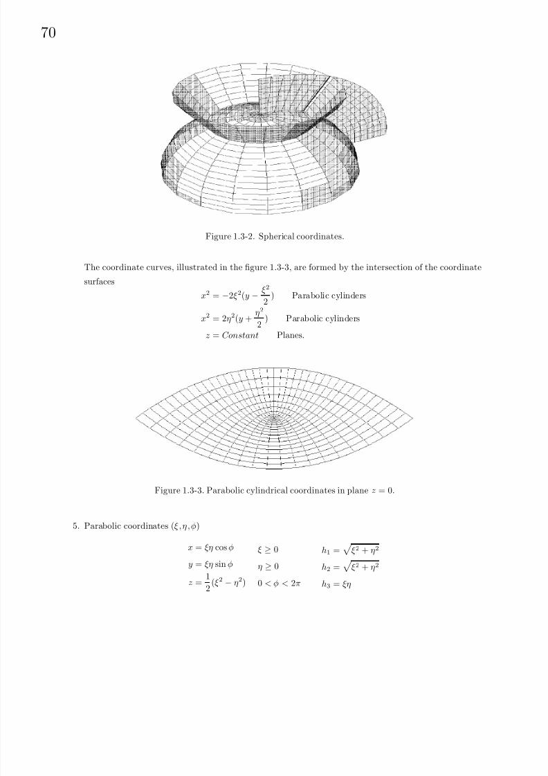
8/6/2019 Introduction to Tensor Calculus Continuum Mechanics - J. Heinbockel
http://slidepdf.com/reader/full/introduction-to-tensor-calculus-continuum-mechanics-j-heinbockel 75/372
70
Figure 1.3-2. Spherical coordinates.
The coordinate curves, illustrated in the figure 1.3-3, are formed by the intersection of the coordinatesurfaces
x2 = −2ξ2(y − ξ2
2) Parabolic cylinders
x2 = 2η2(y +η2
2) Parabolic cylinders
z = Constant Planes.
Figure 1.3-3. Parabolic cylindrical coordinates in plane z = 0.
5. Parabolic coordinates (ξ, η, φ)
x = ξη cos φ
y = ξη sin φ
z =1
2(ξ2 − η2)
ξ ≥ 0
η ≥ 0
0 < φ < 2π
h1 = ξ2 + η2
h2 =
ξ2 + η2
h3 = ξη

8/6/2019 Introduction to Tensor Calculus Continuum Mechanics - J. Heinbockel
http://slidepdf.com/reader/full/introduction-to-tensor-calculus-continuum-mechanics-j-heinbockel 76/372
71
The coordinate curves, illustrated in the figure 1.3-4, are formed by the intersection of the coordinate
surfaces
x2 + y2 = −2ξ2(z − ξ2
2) Paraboloids
x2 + y2 = 2η2(z +η2
2) Paraboloids
y = x tan φ Planes.
Figure 1.3-4. Parabolic coordinates, φ = π/4.
6. Elliptic cylindrical coordinates (ξ, η, z)
x = cosh ξ cos η
y = sinh ξ sin η
z = z
ξ ≥ 0
0 ≤ η ≤ 2π
−∞ < z < ∞
h1 =
sinh2 ξ + sin2 η
h2 =
sinh2 ξ + sin2 η
h3 = 1
The coordinate curves, illustrated in the figure 1.3-5, are formed by the intersection of the coordinatesurfaces
x2
cosh2 ξ+
y2
sinh2 ξ= 1 Elliptic cylinders
x2
cos2 η− y2
sin2 η= 1 Hyperbolic cylinders
z = Constant Planes.

8/6/2019 Introduction to Tensor Calculus Continuum Mechanics - J. Heinbockel
http://slidepdf.com/reader/full/introduction-to-tensor-calculus-continuum-mechanics-j-heinbockel 77/372
72
Figure 1.3-5. Elliptic cylindrical coordinates in the plane z = 0.
7. Elliptic coordinates (ξ, η, φ)
x =
(1− η2)(ξ2 − 1) cos φ
y =
(1− η2)(ξ2 − 1)sin φ
z = ξη
1 ≤ ξ < ∞− 1 ≤ η ≤ 1
0 ≤ φ < 2π
h1 =
ξ2 − η2
ξ2 − 1
h2 =
ξ2 − η2
1 − η2
h3 = (1−
η2)(ξ2
−1)
The coordinate curves, illustrated in the figure 1.3-6, are formed by the intersection of the coordinate
surfacesx2
ξ2 − 1+
y2
ξ2 − 1+
z2
ξ2= 1 Prolate ellipsoid
z2
η2− x2
1 − η2− y2
1 − η2= 1 Two-sheeted hyperboloid
y = x tan φ Planes
8. Bipolar coordinates (u, v, z)
x =a sinh v
cosh v − cos u
, 0
≤u < 2π
y =a sin u
cosh v − cos u, −∞ < v < ∞
z = z −∞ < z < ∞
h21 = h2
2
h22 =
a2
(cosh v − cos u)2
h23 = 1
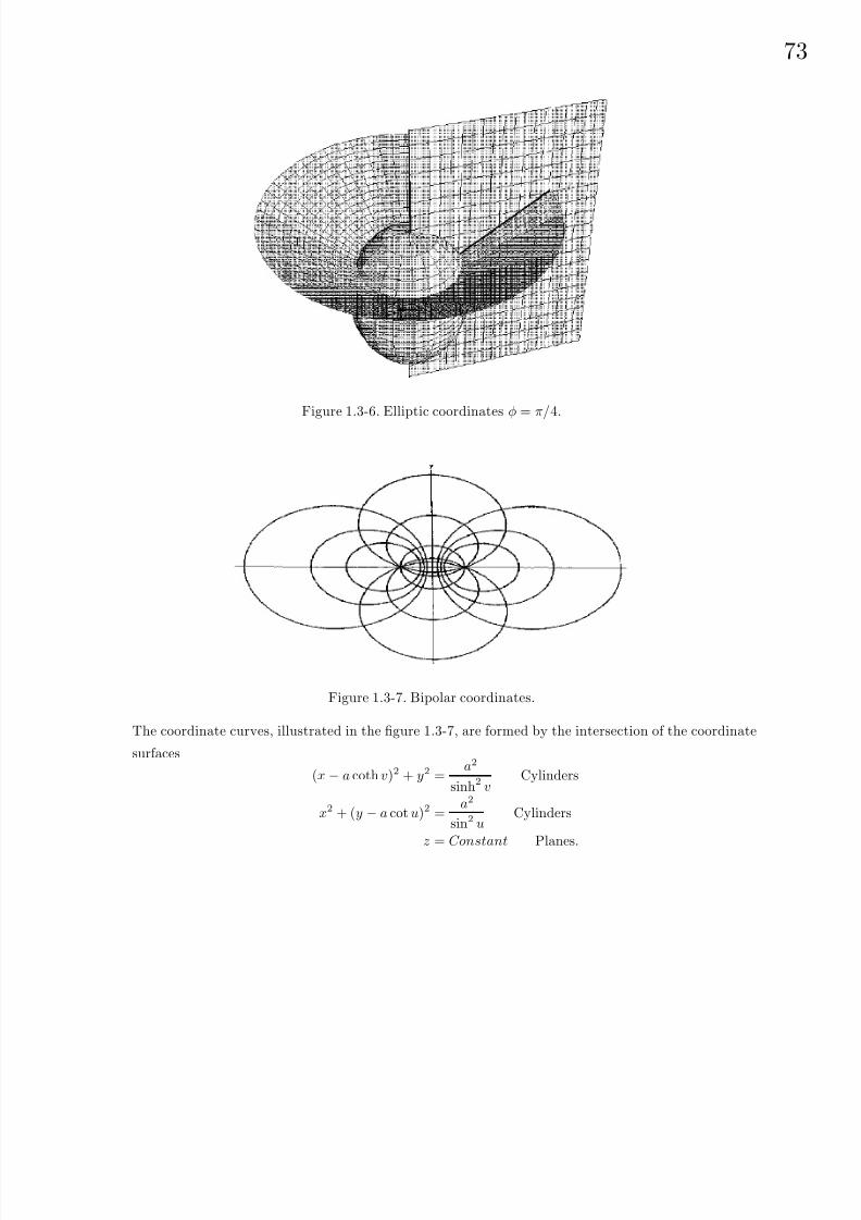
8/6/2019 Introduction to Tensor Calculus Continuum Mechanics - J. Heinbockel
http://slidepdf.com/reader/full/introduction-to-tensor-calculus-continuum-mechanics-j-heinbockel 78/372
73
Figure 1.3-6. Elliptic coordinates φ = π/4.
Figure 1.3-7. Bipolar coordinates.
The coordinate curves, illustrated in the figure 1.3-7, are formed by the intersection of the coordinate
surfaces
(x − a coth v)2 + y2 =a2
sinh2 vCylinders
x2 + (y − a cot u)2 =a2
sin2 uCylinders
z = Constant Planes.

8/6/2019 Introduction to Tensor Calculus Continuum Mechanics - J. Heinbockel
http://slidepdf.com/reader/full/introduction-to-tensor-calculus-continuum-mechanics-j-heinbockel 79/372
74
9. Conical coordinates (u, v, w)
x =uvw
ab, b2 > v2 > a2 > w2, u ≥ 0
y =u
a
(v2 − a2)(w2 − a2)
a2 − b2
z = ub (v2 − b2)(w2 − b2)
b2 − a2
h21 = 1
h22 =
u2(v2 − w2)
(v2 − a2)(b2 − v2)
h23 = u
2
(v2
− w2
)(w2 − a2)(w2 − b2)
The coordinate curves, illustrated in the figure 1.3-8, are formed by the intersection of the coordinate
surfacesx2 + y2 + z2 = u2 Spheres
x2
v2+
y2
v2 − a2+
z2
v2 − b2=0, Cones
x2
w2+
y2
w2 − a2+
z2
w2 − b2= 0, Cones.
Figure 1.3-8. Conical coordinates.
10. Prolate spheroidal coordinates (u, v, φ)
x = a sinh u sin v cos φ, u ≥ 0
y = a sinh u sin v sin φ, 0 ≤ v ≤ π
z = a cosh u cos v, 0
≤φ < 2π
h21 = h2
2
h22 = a2(sinh2 u + sin2 v)
h23 = a2 sinh2 u sin2 v
The coordinate curves, illustrated in the figure 1.3-9, are formed by the intersection of the coordinate
surfacesx2
(a sinh u)2+
y2
(a sinh u)2+
z2
(a cosh u)2= 1, Prolate ellipsoids
z2
(a cos v)2− x2
(a sin v)2− y2
(a sin v)2= 1, Two-sheeted hyperboloid
y = x tan φ, Planes.

8/6/2019 Introduction to Tensor Calculus Continuum Mechanics - J. Heinbockel
http://slidepdf.com/reader/full/introduction-to-tensor-calculus-continuum-mechanics-j-heinbockel 80/372
75
Figure 1.3-9. Prolate spheroidal coordinates
11. Oblate spheroidal coordinates (ξ, η, φ)
x = a cosh ξ cos η cos φ, ξ ≥ 0
y = a cosh ξ cos η sin φ, −π
2≤ η ≤ π
2z = a sinh ξ sin η, 0 ≤ φ ≤ 2π
h21 = h2
2
h22 = a2(sinh2 ξ + sin2 η)
h23 = a2 cosh2 ξ cos2 η
The coordinate curves, illustrated in the figure 1.3-10, are formed by the intersection of the coordinate
surfacesx2
(a cosh ξ)2+
y2
(a cosh ξ)2+
z2
(a sinh ξ)2= 1, Oblate ellipsoids
x2
(a cos η)2+
y2
(a cos η)2− z2
(a sin η)2= 1, One-sheet hyperboloids
y = x tan φ, Planes.
12. Toroidal coordinates (u, v, φ)
x =a sinh v cos φ
cosh v − cos u, 0 ≤ u < 2π
y =a sinh v sin φ
cosh v − cos u, −∞ < v < ∞
z =a sin u
cosh v − cos u, 0 ≤ φ < 2π
h21 = h2
2
h22 =
a2
(cosh v − cos u)2
h23 =
a2 sinh2 v
(cosh v − cos u)2
The coordinate curves, illustrated in the figure 1.3-11, are formed by the intersection of the coordinate
surfaces
x2 + y2 +
z − a cos u
sin u
2=
a2
sin2 u, Spheres
x2 + y2 − acosh v
sinh v
2
+ z2 =a2
sinh2 v, Torus
y = x tan φ, planes
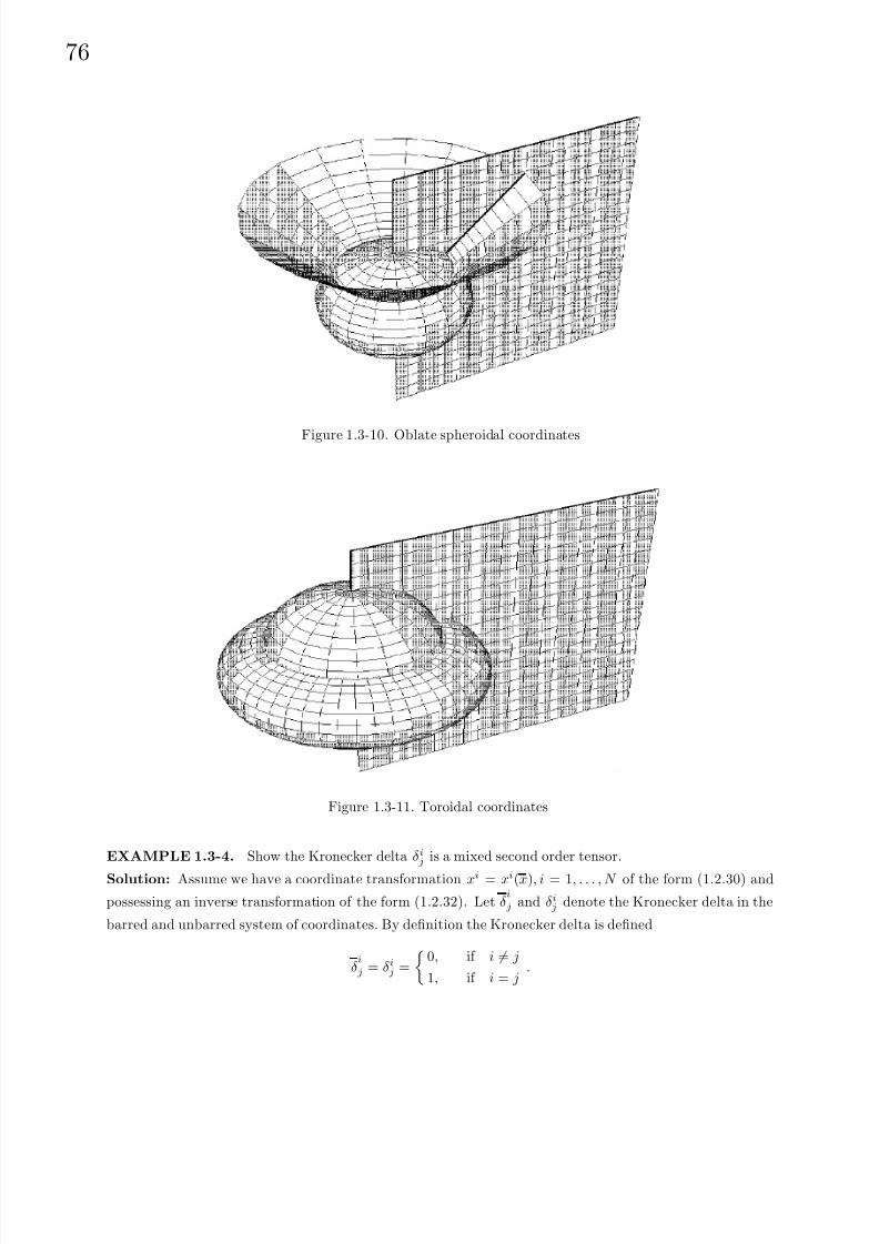
8/6/2019 Introduction to Tensor Calculus Continuum Mechanics - J. Heinbockel
http://slidepdf.com/reader/full/introduction-to-tensor-calculus-continuum-mechanics-j-heinbockel 81/372
76
Figure 1.3-10. Oblate spheroidal coordinates
Figure 1.3-11. Toroidal coordinates
EXAMPLE 1.3-4. Show the Kronecker delta δij is a mixed second order tensor.
Solution: Assume we have a coordinate transformation xi = xi(x), i = 1, . . . , N of the form (1.2.30) and
possessing an inverse transformation of the form (1.2.32). Let δi
j and δij denote the Kronecker delta in the
barred and unbarred system of coordinates. By definition the Kronecker delta is defined
δi
j = δij =
0, if i = j
1, if i = j.

8/6/2019 Introduction to Tensor Calculus Continuum Mechanics - J. Heinbockel
http://slidepdf.com/reader/full/introduction-to-tensor-calculus-continuum-mechanics-j-heinbockel 82/372
77
Employing the chain rule we write
∂xm
∂xn =∂xm
∂xi
∂xi
∂xn =∂xm
∂xi
∂xk
∂xn δik (1.3.14)
By hypothesis, the xi, i = 1, . . . , N are independent coordinates and therefore we have ∂xm
∂xn= δ
m
n and (1.3.14)
simplifies to
δm
n = δik∂xm
∂xi
∂xk
∂xn .
Therefore, the Kronecker delta transforms as a mixed second order tensor.
Conjugate Metric Tensor
Let g denote the determinant of the matrix having the metric tensor gij , i , j = 1, . . . , N as its elements.
In our study of cofactor elements of a matrix we have shown that
cof (g1j)g1k + cof (g2j)g2k + . . . + cof (gNj )gNk = gδjk. (1.3.15)
We can use this fact to find the elements in the inverse matrix associated with the matrix having the
components gij. The elements of this inverse matrix are
gij =1
gcof (gij) (1.3.16)
and are called the conjugate metric components. We examine the summation gijgik and find:
gijgik = g1jg1k + g2jg2k + . . . + gNj gNk
=1
g[cof (g1j)g1k + cof (g2j)g2k + . . . + cof (gNj )gNk ]
=1
g
gδjk
= δjk
The equation
gijgik = δjk (1.3.17)
is an example where we can use the quotient law to show gij is a second order contravariant tensor. Because
of the symmetry of gij and gij the equation (1.3.17) can be represented in other forms.
EXAMPLE 1.3-5. Let Ai and Ai denote respectively the covariant and contravariant components of a
vector A. Show these components are related by the equations
Ai = gijAj (1.3.18)
Ak = gjkAj (1.3.19)
where gij and gij are the metric and conjugate metric components of the space.
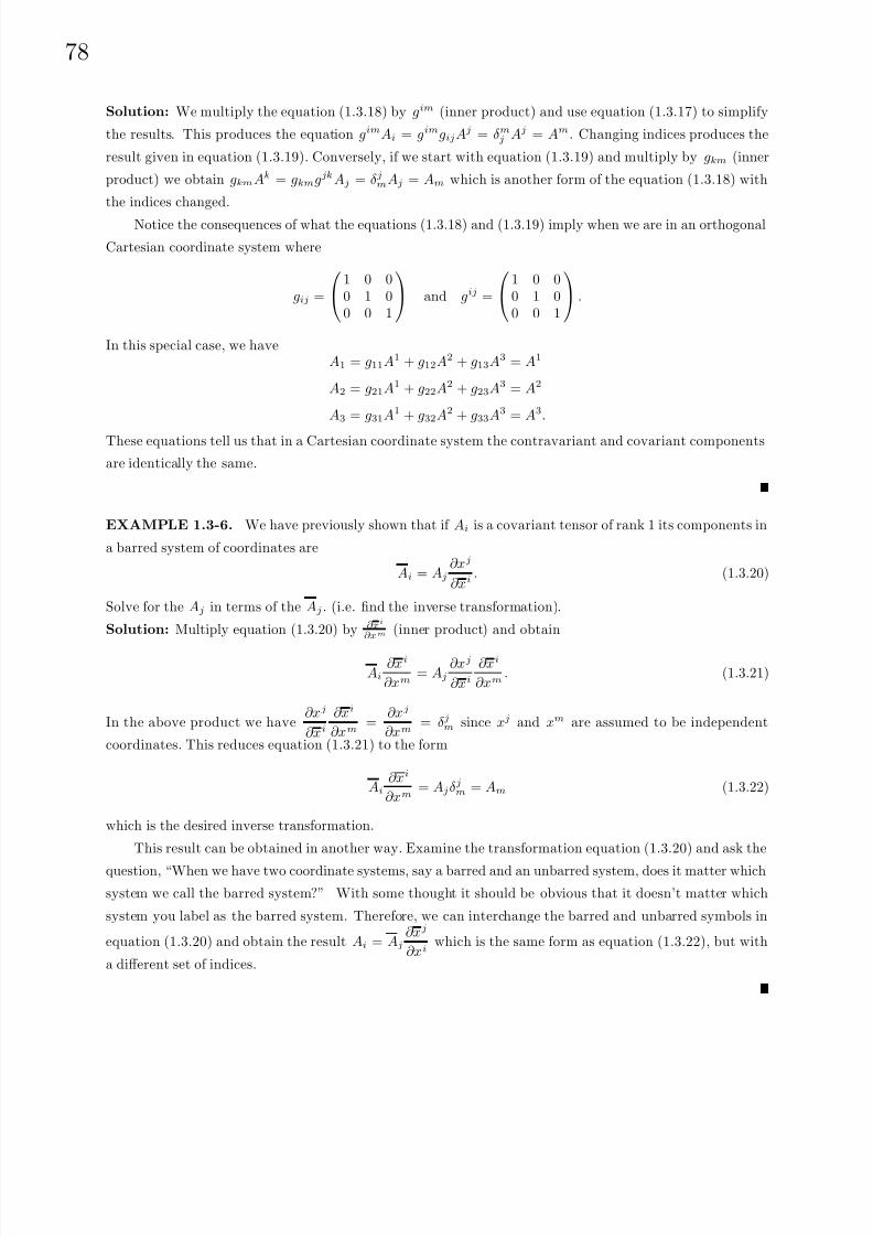
8/6/2019 Introduction to Tensor Calculus Continuum Mechanics - J. Heinbockel
http://slidepdf.com/reader/full/introduction-to-tensor-calculus-continuum-mechanics-j-heinbockel 83/372
78
Solution: We multiply the equation (1.3.18) by gim (inner product) and use equation (1.3.17) to simplify
the results. This produces the equation gimAi = gimgijAj = δmj Aj = Am. Changing indices produces the
result given in equation (1.3.19). Conversely, if we start with equation (1.3.19) and multiply by gkm (inner
product) we obtain gkmAk = gkmgjkAj = δjmAj = Am which is another form of the equation (1.3.18) with
the indices changed.
Notice the consequences of what the equations (1.3.18) and (1.3.19) imply when we are in an orthogonal
Cartesian coordinate system where
gij =
1 0 00 1 00 0 1
and gij =
1 0 00 1 00 0 1
.
In this special case, we haveA1 = g11A1 + g12A2 + g13A3 = A1
A2 = g21A1 + g22A2 + g23A3 = A2
A3 = g31A1 + g32A2 + g33A3 = A3.
These equations tell us that in a Cartesian coordinate system the contravariant and covariant components
are identically the same.
EXAMPLE 1.3-6. We have previously shown that if Ai is a covariant tensor of rank 1 its components in
a barred system of coordinates are
Ai = Aj
∂xj
∂xi. (1.3.20)
Solve for the Aj in terms of the Aj . (i.e. find the inverse transformation).
Solution: Multiply equation (1.3.20) by ∂xi
∂xm(inner product) and obtain
Ai
∂xi
∂xm= Aj
∂xj
∂xi
∂xi
∂xm. (1.3.21)
In the above product we have∂xj
∂xi
∂xi
∂xm=
∂xj
∂xm= δjm since xj and xm are assumed to be independent
coordinates. This reduces equation (1.3.21) to the form
Ai
∂xi
∂xm= Ajδjm = Am (1.3.22)
which is the desired inverse transformation.
This result can be obtained in another way. Examine the transformation equation (1.3.20) and ask the
question, “When we have two coordinate systems, say a barred and an unbarred system, does it matter which
system we call the barred system?” With some thought it should be obvious that it doesn’t matter which
system you label as the barred system. Therefore, we can interchange the barred and unbarred symbols in
equation (1.3.20) and obtain the result Ai = Aj
∂xj
∂xiwhich is the same form as equation (1.3.22), but with
a different set of indices.
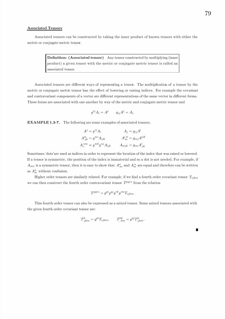
8/6/2019 Introduction to Tensor Calculus Continuum Mechanics - J. Heinbockel
http://slidepdf.com/reader/full/introduction-to-tensor-calculus-continuum-mechanics-j-heinbockel 84/372
79
Associated Tensors
Associated tensors can be constructed by taking the inner product of known tensors with either the
metric or conjugate metric tensor.
Definition: (Associated tensor) Any tensor constructed by multiplying (inner
product) a given tensor with the metric or conjugate metric tensor is called an
associated tensor.
Associated tensors are different ways of representing a tensor. The multiplication of a tensor by the
metric or conjugate metric tensor has the effect of lowering or raising indices. For example the covariant
and contravariant components of a vector are different representations of the same vector in different forms.
These forms are associated with one another by way of the metric and conjugate metric tensor and
gijAi = Aj gijAj = Ai.
EXAMPLE 1.3-7. The following are some examples of associated tensors.
Aj = gijAi
Am.jk = gmiAijk
A.nmi.. = gmkgnjAijk
Aj = gijAi
Ai.km = gmjAijk
Amjk = gimAi.jk
Sometimes ‘dots’are used as indices in order to represent the location of the index that was raised or lowered.
If a tensor is symmetric, the position of the index is immaterial and so a dot is not needed. For example, if
Amn is a symmetric tensor, then it is easy to show that An
.m
and A.n
m
are equal and therefore can be written
as Anm without confusion.
Higher order tensors are similarly related. For example, if we find a fourth order covariant tensor T ijkm
we can then construct the fourth order contravariant tensor T pqrs from the relation
T pqrs = g pigqjgrkgsmT ijkm.
This fourth order tensor can also be expressed as a mixed tensor. Some mixed tensors associated with
the given fourth order covariant tensor are:
T p.jkm = g piT ijkm, T pq..km = gqjT p.jkm.

8/6/2019 Introduction to Tensor Calculus Continuum Mechanics - J. Heinbockel
http://slidepdf.com/reader/full/introduction-to-tensor-calculus-continuum-mechanics-j-heinbockel 85/372
80
Riemann Space V N
A Riemannian space V N is said to exist if the element of arc length squared has the form
ds2 = gijdxidxj (1.3.23)
where the metrices gij = gij(x1, x2, . . . , xN ) are continuous functions of the coordinates and are different
from constants. In the special case gij = δij the Riemannian space V N reduces to a Euclidean space E N .
The element of arc length squared defined by equation (1.3.23) is called the Riemannian metric and any
geometry which results by using this metric is called a Riemannian geometry. A space V N is called flat if
it is possible to find a coordinate transformation where the element of arclength squared is ds2 = i(dxi)2
where each i is either +1 or −1. A space which is not flat is called curved.
Geometry in V N
Given two vectors A = Ai E i and B = Bj E j , then their dot product can be represented
A · B = AiBj E i · E j = gijAiBj = AjBj = AiBi = gijAjBi = | A|| B| cos θ. (1.3.24)
Consequently, in an N dimensional Riemannian space V N the dot or inner product of two vectors A and B
is defined:
gijAiBj = AjBj = AiBi = gijAjBi = AB cos θ. (1.3.25)
In this definition A is the magnitude of the vector Ai, the quantity B is the magnitude of the vector Bi and
θ is the angle between the vectors when their origins are made to coincide. In the special case that θ = 90
we have gijAiBj = 0 as the condition that must be satisfied in order that the given vectors Ai and Bi are
orthogonal to one another. Consider also the special case of equation (1.3.25) when Ai = Bi and θ = 0. In
this case the equations (1.3.25) inform us that
ginAnAi = AiAi = ginAiAn = (A)2. (1.3.26)
From this equation one can determine the magnitude of the vector Ai. The magnitudes A and B can be
written A = (ginAiAn)1
2 and B = (g pqB pBq)1
2 and so we can express equation (1.3.24) in the form
cos θ =gijAiBj
(gmnAmAn)1
2 (g pqB pBq)1
2
. (1.3.27)
An import application of the above concepts arises in the dynamics of rigid body motion. Note that if a
vector A
i
has constant magnitude and the magnitude of
dAi
dt is different from zero, then the vectors A
i
anddAi
dtmust be orthogonal to one another due to the fact that gijAi dA
j
dt= 0. As an example, consider the unit
vectors e1, e2 and e3 on a rotating system of Cartesian axes. We have for constants ci, i = 1, 6 that
d e1dt
= c1 e2 + c2 e3 d e2dt
= c3 e3 + c4 e1 d e3dt
= c5 e1 + c6 e2because the derivative of any ei (i fixed) constant vector must lie in a plane containing the vectors ej and ek, ( j = i , k = i and j = k), since any vector in this plane must be perpendicular to ei.

8/6/2019 Introduction to Tensor Calculus Continuum Mechanics - J. Heinbockel
http://slidepdf.com/reader/full/introduction-to-tensor-calculus-continuum-mechanics-j-heinbockel 86/372
81
The above definition of a dot product in V N can be used to define unit vectors in V N .
Definition: (Unit vector) Whenever the magnitude of a vec-
tor Ai is unity, the vector is called a unit vector. In this case we
havegijAiAj = 1. (1.3.28)
EXAMPLE 1.3-8. (Unit vectors)
In V N the element of arc length squared is expressed ds2 = gij dxidxj which can be expressed in the
form 1 = gijdxi
ds
dxj
ds. This equation states that the vector
dxi
ds, i = 1, . . . , N is a unit vector. One application
of this equation is to consider a particle moving along a curve in V N which is described by the parametric
equations xi = xi(t), for i = 1, . . . , N . The vector V i = dxi
dt
, i = 1, . . . , N represents a velocity vector of the
particle. By chain rule differentiation we have
V i =dxi
dt=
dxi
ds
ds
dt= V
dxi
ds, (1.3.29)
where V = dsdt
is the scalar speed of the particle and dxi
dsis a unit tangent vector to the curve. The equation
(1.3.29) shows that the velocity is directed along the tangent to the curve and has a magnitude V. That isds
dt
2
= (V )2 = gijV iV j .
EXAMPLE 1.3-9. (Curvilinear coordinates)
Find an expression for the cosine of the angles between the coordinate curves associated with the
transformation equations
x = x(u, v, w), y = y(u, v, w), z = z(u, v, w).

8/6/2019 Introduction to Tensor Calculus Continuum Mechanics - J. Heinbockel
http://slidepdf.com/reader/full/introduction-to-tensor-calculus-continuum-mechanics-j-heinbockel 87/372
82
Figure 1.3-12. Angles between curvilinear coordinates.
Solution: Let y1 = x, y2 = y, y3 = z and x1 = u, x2 = v, x3 = w denote the Cartesian and curvilinear
coordinates respectively. With reference to the figure 1.3-12 we can interpret the intersection of the surfaces
v = c2 and w = c3 as the curve r = r(u, c2, c3) which is a function of the parameter u. By moving only along
this curve we have dr =∂r
∂u du and consequently
ds2 = dr · dr =∂r
∂u· ∂r
∂ududu = g11(dx1)2,
or
1 =dr
ds· dr
ds= g11
dx1
ds
2
.
This equation shows that the vector dx1
ds= 1√
g11is a unit vector along this curve. This tangent vector can
be represented by tr(1) = 1√ g11
δr1 .
The curve which is defined by the intersection of the surfaces u = c1 and w = c3 has the unit tangent
vector tr(2) = 1√ g22
δr2. Similarly, the curve which is defined as the intersection of the surfaces u = c1 and
v = c2 has the unit tangent vector tr(3) = 1√ g33 δr3 . The cosine of the angle θ12, which is the angle between the
unit vectors tr(1) and tr(2), is obtained from the result of equation (1.3.25). We find
cos θ12 = g pqt p(1)tq(2) = g pq1√g11
δ p11√g22
δq2 =g12√
g11√
g22.
For θ13 the angle between the directions ti(1) and ti(3) we find
cos θ13 =g13√
g11√
g33.
Finally, for θ23 the angle between the directions ti(2) and ti(3) we find
cos θ23 =g23
√g22√
g33
.
When θ13 = θ12 = θ23 = 90, we have g12 = g13 = g23 = 0 and the coordinate curves which make up the
curvilinear coordinate system are orthogonal to one another.
In an orthogonal coordinate system we adopt the notation
g11 = (h1)2, g22 = (h2)2, g33 = (h3)2 and gij = 0, i = j.
8/6/2019 Introduction to Tensor Calculus Continuum Mechanics - J. Heinbockel
http://slidepdf.com/reader/full/introduction-to-tensor-calculus-continuum-mechanics-j-heinbockel 88/372
83
Epsilon Permutation Symbol
Associated with the e−permutation symbols there are the epsilon permutation symbols defined by the
relations
ijk =√
geijk and ijk =1√
geijk (1.3.30)
where g is the determinant of the metrices gij.
It can be demonstrated that the eijk permutation symbol is a relative tensor of weight −1 whereas the
ijk permutation symbol is an absolute tensor. Similarly, the eijk permutation symbol is a relative tensor of
weight +1 and the corresponding ijk permutation symbol is an absolute tensor.
EXAMPLE 1.3-10. ( permutation symbol)
Show that eijk is a relative tensor of weight −1 and the corresponding ijk permutation symbol is an
absolute tensor.
Solution: Examine the Jacobian
J x
x =
∂x1
∂x1∂x1
∂x2∂x1
∂x3
∂x2
∂x1∂x2
∂x2∂x2
∂x3
∂x3
∂x1∂x
3
∂x2∂x
3
∂x3
and make the substitution
aij =∂xi
∂xj, i, j = 1, 2, 3.
From the definition of a determinant we may write
eijkaimajnak p = J (x
x)emnp. (1.3.31)
By definition, emnp = emnp in all coordinate systems and hence equation (1.3.31) can be expressed in the
form
J (x
x
)−1
eijk∂xi
∂xm
∂xj
∂xn
∂xk
∂x p = emnp (1.3.32)
which demonstrates that eijk transforms as a relative tensor of weight −1.
We have previously shown the metric tensor gij is a second order covariant tensor and transforms
according to the rule gij = gmn
∂xm
∂xi
∂xn
∂xj. Taking the determinant of this result we find
g = |gij | = |gmn|∂xm
∂xi
2 = g
J (x
x)2
(1.3.33)
where g is the determinant of (gij) and g is the determinant of (gij). This result demonstrates that g is a
scalar invariant of weight +2. Taking the square root of this result we find that
g = √gJ (x
x ). (1.3.34)
Consequently, we call√
g a scalar invariant of weight +1. Now multiply both sides of equation (1.3.32) by√
g and use (1.3.34) to verify the relation
√g eijk
∂xi
∂xm
∂xj
∂xn
∂xk
∂x p=
g emnp. (1.3.35)
This equation demonstrates that the quantity ijk =√
g eijk transforms like an absolute tensor.

8/6/2019 Introduction to Tensor Calculus Continuum Mechanics - J. Heinbockel
http://slidepdf.com/reader/full/introduction-to-tensor-calculus-continuum-mechanics-j-heinbockel 89/372
84
Figure 1.3-14. Translation followed by rotation of axes
In a similar manner one can show eijk is a relative tensor of weight +1 and ijk = 1√ g
eijk is an absolute
tensor. This is left as an exercise.
Another exercise found at the end of this section is to show that a generalization of the e − δ identityis the epsilon identity
gijiptjrs = g prgts − g psgtr. (1.3.36)
Cartesian Tensors
Consider the motion of a rigid rod in two dimensions. No matter how complicated the movement of
the rod is we can describe the motion as a translation followed by a rotation. Consider the rigid rod AB
illustrated in the figure 1.3-13.
Figure 1.3-13. Motion of rigid rod
In this figure there is a before and after picture of the rod’s position. By moving the point B to B we
have a translation. This is then followed by a rotation holding B fixed.

8/6/2019 Introduction to Tensor Calculus Continuum Mechanics - J. Heinbockel
http://slidepdf.com/reader/full/introduction-to-tensor-calculus-continuum-mechanics-j-heinbockel 90/372
85
Figure 1.3-15. Rotation of axes
A similar situation exists in three dimensions. Consider two sets of Cartesian axes, say a barred and
unbarred system as illustrated in the figure 1.3-14. Let us translate the origin 0 to 0 and then rotate the
(x, y, z) axes until they coincide with the (x, y, z) axes. We consider first the rotation of axes when theorigins 0 and 0 coincide as the translational distance can be represented by a vector bk, k = 1, 2, 3. When
the origin 0 is translated to 0 we have the situation illustrated in the figure 1.3-15, where the barred axes
can be thought of as a transformation due to rotation.
Let
r = x e1 + y e2 + z e3 (1.3.37)
denote the position vector of a variable point P with coordinates (x, y, z) with respect to the origin 0 and the
unit vectors e1, e2, e3. This same point, when referenced with respect to the origin 0 and the unit vectors
e1, e2, e3, has the representation
r = x e1 + y e2 + z e3. (1.3.38)
By considering the projections of r upon the barred and unbarred axes we can construct the transformation
equations relating the barred and unbarred axes. We calculate the projections of r onto the x, y and z axes
and find:r · e1 = x = x( e1 · e1) + y( e2 · e1) + z( e3 · e1)
r · e2 = y = x( e1 · e2) + y( e2 · e2) + z( e3 · e2)
r · e3 = z = x( e1 · e3) + y( e2 · e3) + z( e3 · e3).
(1.3.39)
We also calculate the projection of r onto the x, y, z axes and find:
r · e1 = x = x(
e1 · e1) + y(
e2 · e1) + z(
e3 · e1)
r · e2 = y = x( e1 · e2) + y( e2 · e2) + z( e3 · e2)
r · e3 = z = x( e1 · e3) + y( e2 · e3) + z( e3 · e3).
(1.3.40)
By introducing the notation (y1, y2, y3) = (x, y, z) (y1, y2, y3) = (x, y, z) and defining θij as the angle
between the unit vectors ei and ej , we can represent the above transformation equations in a more concise
8/6/2019 Introduction to Tensor Calculus Continuum Mechanics - J. Heinbockel
http://slidepdf.com/reader/full/introduction-to-tensor-calculus-continuum-mechanics-j-heinbockel 91/372
86
form. We observe that the direction cosines can be written as
11 = e1 · e1 = cos θ11
21 = e2 · e1 = cos θ21
31 = e3 · e1 = cos θ31
12 = e1 · e2 = cos θ12
22 = e2 · e2 = cos θ22
32 = e3 · e2 = cos θ32
13 = e1 · e3 = cos θ13
23 = e2 · e3 = cos θ23
33 = e3 · e3 = cos θ33
(1.3.41)
which enables us to write the equations (1.3.39) and (1.3.40) in the form
yi = ijyj and yi = jiyj . (1.3.42)
Using the index notation we represent the unit vectors as:
er = pr e p or e p = pr er (1.3.43)
where pr are the direction cosines. In both the barred and unbarred system the unit vectors are orthogonal
and consequently we must have the dot products
er · e p = δrp and em · en = δmn (1.3.44)
where δij is the Kronecker delta. Substituting equation (1.3.43) into equation (1.3.44) we find the direction
cosines ij must satisfy the relations:
er · es = pr e p · ms em = prms e p · em = prmsδ pm = mrms = δrs
and er · es = rm em · sn en = rmsn em · en = rmsnδmn = rmsm = δrs.
The relations
mrms = δrs and rmsm = δrs, (1.3.45)
with summation index m, are important relations which are satisfied by the direction cosines associated with
a rotation of axes.
Combining the rotation and translation equations we find
yi = ijyj rotation
+ bi translation
. (1.3.46)
We multiply this equation by ik and make use of the relations (1.3.45) to find the inverse transformation
yk = ik(yi − bi). (1.3.47)
These transformations are called linear or affine transformations.
Consider the xi axes as fixed, while the xi axes are rotating with respect to the xi axes where both sets
of axes have a common origin. Let A = Ai ei denote a vector fixed in and rotating with the xi axes. We
denote byd A
dt
f
andd A
dt
r
the derivatives of A with respect to the fixed (f) and rotating (r) axes. We can

8/6/2019 Introduction to Tensor Calculus Continuum Mechanics - J. Heinbockel
http://slidepdf.com/reader/full/introduction-to-tensor-calculus-continuum-mechanics-j-heinbockel 92/372
87
write, with respect to the fixed axes, thatd A
dt
f
=dAi
dtei + Ai d ei
dt. Note that
d eidt
is the derivative of a
vector with constant magnitude. Therefore there exists constants ωi, i = 1, . . . , 6 such that
d
e1
dt= ω3
e2 − ω2
e3
d
e2
dt= ω1
e3 − ω4
e1
d
e3
dt= ω5
e1 − ω6
e2
i.e. see page 80. From the dot product e1 · e2 = 0 we obtain by differentiation e1 · d e2dt
+ d e1dt
· e2 = 0
which implies ω4 = ω3. Similarly, from the dot products e1 · e3 and e2 · e3 we obtain by differentiation the
additional relations ω5 = ω2 and ω6 = ω1. The derivative of A with respect to the fixed axes can now be
represented
d A
dt
f
=dAi
dtei + (ω2A3 − ω3A2) e1 + (ω3A1 − ω1A3) e2 + (ω1A2 − ω2A1) e3 =
d A
dt
r
+ ω × A
where ω = ωi ei is called an angular velocity vector of the rotating system. The term ω × A represents the
velocity of the rotating system relative to the fixed system andd A
dt
r
=dAi
dt
ei represents the derivative with
respect to the rotating system.Employing the special transformation equations (1.3.46) let us examine how tensor quantities transform
when subjected to a translation and rotation of axes. These are our special transformation laws for Cartesian
tensors. We examine only the transformation laws for first and second order Cartesian tensor as higher order
transformation laws are easily discerned. We have previously shown that in general the first and second order
tensor quantities satisfy the transformation laws:
Ai = Aj
∂yj
∂y i
(1.3.48)
Ai
= Aj ∂y i
∂yj
(1.3.49)
Amn
= Aij
∂ym∂yi
∂yn∂yj
(1.3.50)
Amn = Aij
∂yi
∂ym
∂yj∂yn
(1.3.51)
Am
n = Aij
∂ym
∂yi
∂yj
∂yn
(1.3.52)
For the special case of Cartesian tensors we assume that yi and yi, i = 1, 2, 3 are linearly independent. We
differentiate the equations (1.3.46) and (1.3.47) and find
∂yi
∂yk
= ij∂yj
∂yk
= ijδjk = ik, and∂yk
∂ym
= ik∂yi
∂ym
= ikδim = mk.
Substituting these derivatives into the transformation equations (1.3.48) through (1.3.52) we produce thetransformation equations
Ai = Ajji
Ai
= Ajji
Amn
= Aijimjn
Amn = Aijimjn
Am
n = Aijimjn.
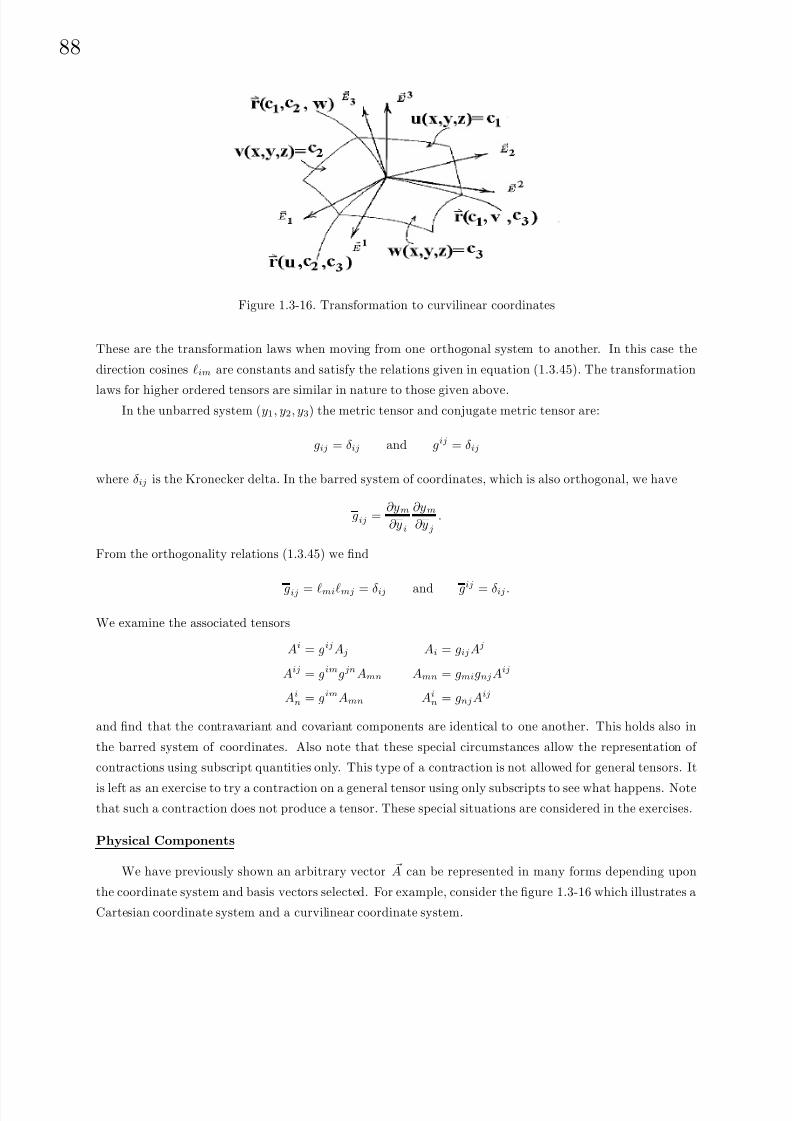
8/6/2019 Introduction to Tensor Calculus Continuum Mechanics - J. Heinbockel
http://slidepdf.com/reader/full/introduction-to-tensor-calculus-continuum-mechanics-j-heinbockel 93/372
88
Figure 1.3-16. Transformation to curvilinear coordinates
These are the transformation laws when moving from one orthogonal system to another. In this case the
direction cosines im are constants and satisfy the relations given in equation (1.3.45). The transformation
laws for higher ordered tensors are similar in nature to those given above.In the unbarred system (y1, y2, y3) the metric tensor and conjugate metric tensor are:
gij = δij and gij = δij
where δij is the Kronecker delta. In the barred system of coordinates, which is also orthogonal, we have
gij =∂ym
∂y i
∂ym
∂yj
.
From the orthogonality relations (1.3.45) we find
gij = mimj = δij and gij
= δij .
We examine the associated tensors
Ai = gijAj
Aij = gimgjnAmn
Ain = gimAmn
Ai = gijAj
Amn = gmignjAij
Ain = gnjAij
and find that the contravariant and covariant components are identical to one another. This holds also in
the barred system of coordinates. Also note that these special circumstances allow the representation of
contractions using subscript quantities only. This type of a contraction is not allowed for general tensors. It
is left as an exercise to try a contraction on a general tensor using only subscripts to see what happens. Note
that such a contraction does not produce a tensor. These special situations are considered in the exercises.
Physical Components
We have previously shown an arbitrary vector A can be represented in many forms depending upon
the coordinate system and basis vectors selected. For example, consider the figure 1.3-16 which illustrates a
Cartesian coordinate system and a curvilinear coordinate system.
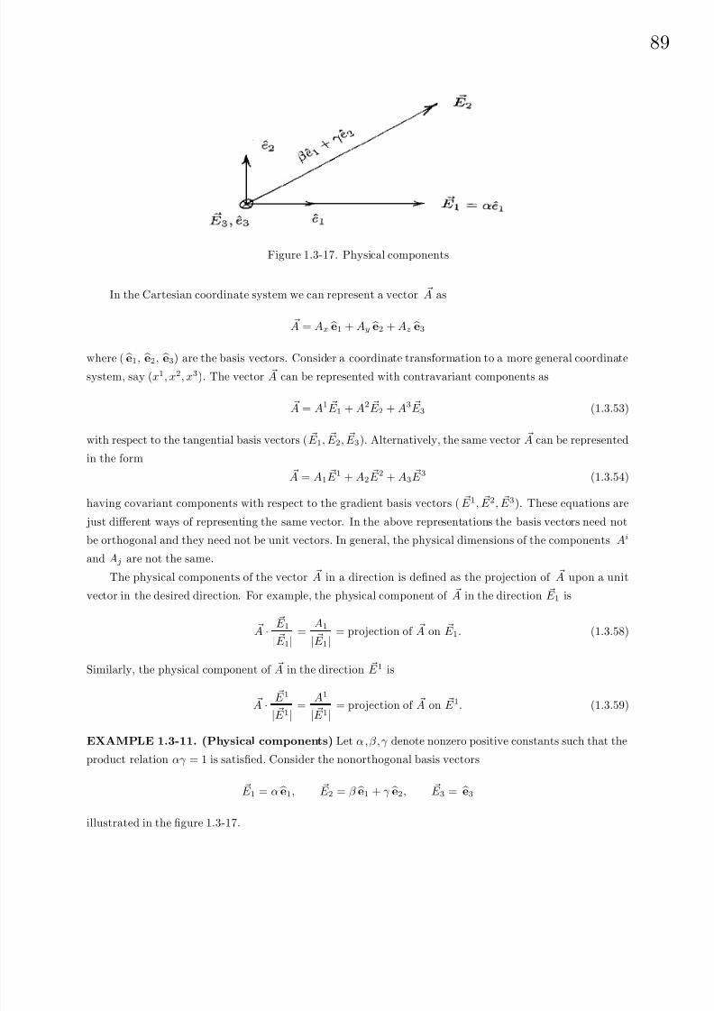
8/6/2019 Introduction to Tensor Calculus Continuum Mechanics - J. Heinbockel
http://slidepdf.com/reader/full/introduction-to-tensor-calculus-continuum-mechanics-j-heinbockel 94/372
89
Figure 1.3-17. Physical components
In the Cartesian coordinate system we can represent a vector A as
A = Ax
e1 + Ay
e2 + Az
e3
where ( e1, e2, e3) are the basis vectors. Consider a coordinate transformation to a more general coordinate
system, say (x1, x2, x3). The vector A can be represented with contravariant components as
A = A1 E 1 + A2 E 2 + A3 E 3 (1.3.53)
with respect to the tangential basis vectors ( E 1, E 2, E 3). Alternatively, the same vector A can be represented
in the form
A = A1 E 1 + A2
E 2 + A3 E 3 (1.3.54)
having covariant components with respect to the gradient basis vectors ( E 1, E 2, E 3). These equations are
just different ways of representing the same vector. In the above representations the basis vectors need not
be orthogonal and they need not be unit vectors. In general, the physical dimensions of the components Ai
and Aj are not the same.
The physical components of the vector A in a direction is defined as the projection of A upon a unit
vector in the desired direction. For example, the physical component of A in the direction E 1 is
A · E 1
| E 1|=
A1
| E 1|= projection of A on E 1. (1.3.58)
Similarly, the physical component of A in the direction E 1 is
A · E 1
| E 1| =
A1
| E 1| = projection of A on E 1
. (1.3.59)
EXAMPLE 1.3-11. (Physical components) Let α, β, γ denote nonzero positive constants such that the
product relation αγ = 1 is satisfied. Consider the nonorthogonal basis vectors
E 1 = α e1, E 2 = β e1 + γ e2, E 3 = e3illustrated in the figure 1.3-17.

8/6/2019 Introduction to Tensor Calculus Continuum Mechanics - J. Heinbockel
http://slidepdf.com/reader/full/introduction-to-tensor-calculus-continuum-mechanics-j-heinbockel 95/372
90
It is readily verified that the reciprocal basis is
E 1 = γ e1 − β e2, E 2 = α e2, E 3 = e3.
Consider the problem of representing the vector A = Ax
e1 + Ay
e2 in the contravariant vector form
A = A1 E 1 + A2 E 2 or tensor form Ai, i = 1, 2.
This vector has the contravariant components
A1 = A · E 1 = γAx − βAy and A2 = A · E 2 = αAy.
Alternatively, this same vector can be represented as the covariant vector
A = A1 E 1 + A2
E 2 which has the tensor form Ai, i = 1, 2.
The covariant components are found from the relations
A1 = A · E 1 = αAx A2 = A · E 2 = βAx + γAy.
The physical components of A in the directions E 1 and E 2 are found to be:
A · E 1
| E 1| =A1
| E 1| =γAx − βAy
γ 2 + β 2= A(1)
A · E 2
| E 2| =A2
| E 2| =αAy
α= Ay = A(2).
Note that these same results are obtained from the dot product relations using either form of the vector A.
For example, we can write
A · E 1
| E 1| =A1( E 1 · E 1) + A2( E 2 · E 1)
| E 1| = A(1)
and A · E 2
| E 2| =A1( E 1 · E 2) + A2( E 2 · E 2)
| E 2| = A(2).
In general, the physical components of a vector A in a direction of a unit vector λi is the generalized
dot product in V N . This dot product is an invariant and can be expressed
gijAi
λj
= Ai
λi = Aiλi
= projection of A in direction of λi

8/6/2019 Introduction to Tensor Calculus Continuum Mechanics - J. Heinbockel
http://slidepdf.com/reader/full/introduction-to-tensor-calculus-continuum-mechanics-j-heinbockel 96/372
91
Physical Components For Orthogonal Coordinates
In orthogonal coordinates observe the element of arc length squared in V 3 is
ds2 = gijdxidxj = (h1)2(dx1)2 + (h2)2(dx2)2 + (h3)2(dx3)2
where
gij =
(h1)2 0 00 (h2)2 00 0 (h3)2
. (1.3.60)
In this case the curvilinear coordinates are orthogonal and
h2(i) = g(i)(i) i not summed and gij = 0, i = j.
At an arbitrary point in this coordinate system we take λi, i = 1, 2, 3 as a unit vector in the direction
of the coordinate x1. We then obtain
λ1 = dx1
ds , λ2 = 0, λ3 = 0.
This is a unit vector since
1 = gijλiλj = g11λ1λ1 = h21(λ1)2
or λ1 = 1h1
. Here the curvilinear coordinate system is orthogonal and in this case the physical component
of a vector Ai, in the direction xi, is the projection of Ai on λi in V 3. The projection in the x1 direction is
determined from
A(1) = gijAiλj = g11A1λ1 = h21A1 1
h1= h1A1.
Similarly, we choose unit vectors µi and ν i, i = 1, 2, 3 in the x2 and x3 directions. These unit vectors
can be represented
µ1 =0,
ν 1 =0,
µ2 =dx2
ds=
1
h2,
ν 2 =0,
µ3 =0
ν 3 =dx3
ds=
1
h3
and the physical components of the vector Ai in these directions are calculated as
A(2) = h2A2 and A(3) = h3A3.
In summary, we can say that in an orthogonal coordinate system the physical components of a contravariant
tensor of order one can be determined from the equations
A(i) = h(i)A(i) =√
g(i)(i)A(i), i = 1, 2 or 3 no summation on i,
which is a short hand notation for the physical components (h1A1, h2A2, h3A3). In an orthogonal coordinate
system the nonzero conjugate metric components are
g(i)(i) =1
g(i)(i), i = 1, 2, or 3 no summation on i.

8/6/2019 Introduction to Tensor Calculus Continuum Mechanics - J. Heinbockel
http://slidepdf.com/reader/full/introduction-to-tensor-calculus-continuum-mechanics-j-heinbockel 97/372
92
These components are needed to calculate the physical components associated with a covariant tensor of
order one. For example, in the x1−direction, we have the covariant components
λ1 = g11λ1 = h21
1
h1= h1, λ2 = 0, λ3 = 0
and consequently the projection in V 3
can be represented
gijAiλj = gijAigjmλm = Ajgjmλm = A1λ1g11 = A1h11
h21
=A1
h1= A(1).
In a similar manner we calculate the relations
A(2) =A2
h2and A(3) =
A3
h3
for the other physical components in the directions x2 and x3. These physical components can be represented
in the short hand notation
A(i) =A(i)
h(i)
=A(i)
√g(i)(i), i = 1, 2 or 3 no summation on i.
In an orthogonal coordinate system the physical components associated with both the contravariant and
covariant components are the same. To show this we note that when Aigij = Aj is summed on i we obtain
A1g1j + A2g2j + A3g3j = Aj .
Since gij = 0 for i = j this equation reduces to
A(i)g(i)(i) = A(i), i not summed.
Another form for this equation is
A(i) = A(i)√g(i)(i) =A(i)√g(i)(i)
i not summed,
which demonstrates that the physical components associated with the contravariant and covariant compo-
nents are identical.
NOTATION The physical components are sometimes expressed by symbols with subscripts which represent
the coordinate curve along which the projection is taken. For example, let H i denote the contravariant
components of a first order tensor. The following are some examples of the representation of the physical
components of H i in various coordinate systems:
orthogonal coordinate tensor physical
coordinates system components components
general (x1, x2, x3) H i H (1), H (2), H (3)
rectangular (x, y, z) H i H x, H y, H z
cylindrical (r,θ,z) H i H r, H θ, H z
spherical (ρ,θ,φ) H i H ρ, H θ, H φ
general (u,v,w) H i H u, H v , H w

8/6/2019 Introduction to Tensor Calculus Continuum Mechanics - J. Heinbockel
http://slidepdf.com/reader/full/introduction-to-tensor-calculus-continuum-mechanics-j-heinbockel 98/372
93
Higher Order Tensors
The physical components associated with higher ordered tensors are defined by projections in V N just
like the case with first order tensors. For an nth ordered tensor T ij...k we can select n unit vectors λi, µi, . . . , ν i
and form the inner product (projection)
T ij...kλ
i
µ
j
. . . ν
k
.
When projecting the tensor components onto the coordinate curves, there are N choices for each of the unit
vectors. This produces N n physical components.
The above inner product represents the physical component of the tensor T ij...k along the directions of
the unit vectors λi, µi, . . . , ν i. The selected unit vectors may or may not be orthogonal. In the cases where
the selected unit vectors are all orthogonal to one another, the calculation of the physical components is
greatly simplified. By relabeling the unit vectors λi(m), λi
(n), . . . , λi( p) where (m), (n), ..., ( p) represent one of
the N directions, the physical components of a general nth order tensor is represented
T (m n . . . p) = T ij...kλi(m)λj
(n). . . λk
( p)
EXAMPLE 1.3-12. (Physical components)
In an orthogonal curvilinear coordinate system V 3 with metric gij , i,j = 1, 2, 3, find the physical com-
ponents of
(i) the second order tensor Aij . (ii) the second order tensor Aij . (iii) the second order tensor Aij .
Solution: The physical components of Amn, m , n = 1, 2, 3 along the directions of two unit vectors λi and
µi is defined as the inner product in V 3. These physical components can be expressed
A(ij) = Amnλm(i)µn
(j) i, j = 1, 2, 3,
where the subscripts (i) and ( j) represent one of the coordinate directions. Dropping the subscripts ( i) and
( j), we make the observation that in an orthogonal curvilinear coordinate system there are three choices for
the direction of the unit vector λi and also three choices for the direction of the unit vector µi. These three
choices represent the directions along the x1, x2 or x3 coordinate curves which emanate from a point of the
curvilinear coordinate system. This produces a total of nine possible physical components associated with
the tensor Amn.
For example, we can obtain the components of the unit vector λi, i = 1, 2, 3 in the x1 direction directly
from an examination of the element of arc length squared
ds2 = (h1)2(dx1)2 + (h2)2(dx2)2 + (h3)2(dx3)2.
By setting dx2
= dx3
= 0, we find
dx1
ds=
1
h1= λ1, λ2 = 0, λ3 = 0.
This is the vector λi(1), i = 1, 2, 3. Similarly, if we choose to select the unit vector λi, i = 1, 2, 3 in the x2
direction, we set dx1 = dx3 = 0 in the element of arc length squared and find the components
λ1 = 0, λ2 =dx2
ds=
1
h2, λ3 = 0.

8/6/2019 Introduction to Tensor Calculus Continuum Mechanics - J. Heinbockel
http://slidepdf.com/reader/full/introduction-to-tensor-calculus-continuum-mechanics-j-heinbockel 99/372
94
This is the vector λi(2), i = 1, 2, 3. Finally, if we select λi, i = 1, 2, 3 in the x3 direction, we set dx1 = dx2 = 0
in the element of arc length squared and determine the unit vector
λ1 = 0, λ2 = 0, λ3 =dx3
ds=
1
h3.
This is the vector λi(3), i = 1, 2, 3. Similarly, the unit vector µi can be selected as one of the above three
directions. Examining all nine possible combinations for selecting the unit vectors, we calculate the physical
components in an orthogonal coordinate system as:
A(11) =A11
h1h1
A(21) =A21
h1h2
A(31) =A31
h3h1
A(12) =A12
h1h2
A(22) =A22
h2h2
A(32) =A32
h3h2
A(13) =A13
h1h3
A(23) =A23
h2h3
A(33) =A33
h3h3
These results can be written in the more compact form
A(ij) =A(i)(j)
h(i)h(j)no summation on i or j . (1.3.61)
For mixed tensors we have
Aij = gimAmj = gi1A1j + gi2A2j + gi3A3j . (1.3.62)
From the fact gij = 0 for i = j, together with the physical components from equation (1.3.61), the equation
(1.3.62) reduces to
A
(i)
(j) = g
(i)(i)
A(i)(j) =
1
h2(i) · h(i)h(j)A(ij) no summation on i and i, j = 1, 2 or 3.
This can also be written in the form
A(ij) = A(i)(j)
h(i)
h(j)no summation on i or j. (1.3.63)
Hence, the physical components associated with the mixed tensor Aij in an orthogonal coordinate system
can be expressed asA(11) = A1
1
A(21) = A21
h2
h1
A(31) = A31
h3
h1
A(12) = A12
h1
h2
A(22) = A22
A(32) = A32
h3
h2
A(13) = A13
h1
h3
A(23) = A23
h2
h3
A(33) = A33.
For second order contravariant tensors we may write
Aijgjm = Aim = Ai1g1m + Ai2g2m + Ai3g3m.
8/6/2019 Introduction to Tensor Calculus Continuum Mechanics - J. Heinbockel
http://slidepdf.com/reader/full/introduction-to-tensor-calculus-continuum-mechanics-j-heinbockel 100/372
95
We use the fact gij = 0 for i = j together with the physical components from equation (1.3.63) to reduce the
above equation to the form A(i)(m) = A(i)(m)g(m)(m) no summation on m . In terms of physical components
we have
h(m)
h(i)A(im) = A(i)(m)h2
(m) or A(im) = A(i)(m)h(i)h(m). no summation i, m = 1, 2, 3 (1.3.64)
Examining the results from equation (1.3.64) we find that the physical components associated with the
contravariant tensor Aij , in an orthogonal coordinate system, can be written as:
A(11) = A11h1h1
A(21) = A21h2h1
A(31) = A31h3h1
A(12) = A12h1h2
A(22) = A22h2h2
A(32) = A32h3h2
A(13) = A13h1h3
A(23) = A23h2h3
A(33) = A33h3h3.
Physical Components in General
In an orthogonal curvilinear coordinate system, the physical components associated with the nth order
tensor T ij...kl along the curvilinear coordinate directions can be represented:
T (ij . . . kl) =T (i)(j)...(k)(l)
h(i)h(j) . . . h(k)h(l)no summations.
These physical components can be related to the various tensors associated with T ij...kl. For example, in
an orthogonal coordinate system, the physical components associated with the mixed tensor T ij...mn...kl can be
expressed as:
T (ij . . . m n . . . kl) = T (i)(j)...(m)(n)...(k)(l)
h(i)h(j) . . . h(m)
h(n) . . . h(k)h(l)no summations. (1.3.65)
EXAMPLE 1.3-13. (Physical components) Let xi = xi(t), i = 1, 2, 3 denote the position vector of a
particle which moves as a function of time t. Assume there exists a coordinate transformation xi = xi(x), for
i = 1, 2, 3, of the form given by equations (1.2.33). The position of the particle when referenced with respect
to the barred system of coordinates can be found by substitution. The generalized velocity of the particle
in the unbarred system is a vector with components
vi =dxi
dt, i = 1, 2, 3.
The generalized velocity components of the same particle in the barred system is obtained from the chain
rule. We find this velocity is represented by
vi =dxi
dt=
∂xi
∂xj
dxj
dt=
∂xi
∂xjvj .
This equation implies that the contravariant quantities
(v1, v2, v3) = (dx1
dt,
dx2
dt,
dx3
dt)

8/6/2019 Introduction to Tensor Calculus Continuum Mechanics - J. Heinbockel
http://slidepdf.com/reader/full/introduction-to-tensor-calculus-continuum-mechanics-j-heinbockel 101/372
96
are tensor quantities. These quantities are called the components of the generalized velocity. The coordinates
x1, x2, x3 are generalized coordinates. This means we can select any set of three independent variables for
the representation of the motion. The variables selected might not have the same dimensions. For example,
in cylindrical coordinates we let (x1 = r, x2 = θ, x3 = z). Here x1 and x3 have dimensions of distance but x2
has dimensions of angular displacement. The generalized velocities are
v1 =dx1
dt=
dr
dt, v2 =
dx2
dt=
dθ
dt, v3 =
dx3
dt=
dz
dt.
Here v1 and v3 have units of length divided by time while v2 has the units of angular velocity or angular
change divided by time. Clearly, these dimensions are not all the same. Let us examine the physical
components of the generalized velocities. We find in cylindrical coordinates h1 = 1, h2 = r, h3 = 1 and the
physical components of the velocity have the forms:
vr = v(1) = v1h1 =dr
dt, vθ = v(2) = v2h2 = r
dθ
dt, vz = v(3) = v3h3 =
dz
dt.
Now the physical components of the velocity all have the same units of length divided by time.
Additional examples of the use of physical components are considered later. For the time being, just
remember that when tensor equations are derived, the equations are valid in any generalized coordinate
system. In particular, we are interested in the representation of physical laws which are to be invariant and
independent of the coordinate system used to represent these laws. Once a tensor equation is derived, we
can chose any type of generalized coordinates and expand the tensor equations. Before using any expanded
tensor equations we must replace all the tensor components by their corresponding physical components in
order that the equations are dimensionally homogeneous. It is these expanded equations, expressed in terms
of the physical components, which are used to solve applied problems.
Tensors and Multilinear Forms
Tensors can be thought of as being created by multilinear forms defined on some vector space V. Let
us define on a vector space V a linear form, a bilinear form and a general multilinear form. We can then
illustrate how tensors are created from these forms.
Definition: (Linear form) Let V denote a vector space which
contains vectors x, x1, x2, . . . . A linear form in x is a scalar function
ϕ(x) having a single vector argument x which satisfies the linearity
properties:
(i) ϕ(x1 + x2) = ϕ( x1) + ϕ(x2)
(ii) ϕ(µ x1) = µϕ( x1)(1.3.66)
for all arbitrary vectors x1, x2 in V and all real numbers µ.
8/6/2019 Introduction to Tensor Calculus Continuum Mechanics - J. Heinbockel
http://slidepdf.com/reader/full/introduction-to-tensor-calculus-continuum-mechanics-j-heinbockel 102/372

8/6/2019 Introduction to Tensor Calculus Continuum Mechanics - J. Heinbockel
http://slidepdf.com/reader/full/introduction-to-tensor-calculus-continuum-mechanics-j-heinbockel 103/372
98
Note in the definition of a bilinear form that the scalar function ϕ is linear in both the arguments x and
y. An example of a bilinear form is the dot product relation
ϕ(x, y) = x · y (1.3.69)
where both x and y belong to the same vector space V.The definition of a bilinear form suggests how multilinear forms can be defined.
Definition: (Multilinear forms) A multilinear form of degree M or a M degree
linear form in the vector arguments
x1, x2, . . . , xM
is a scalar function
ϕ(x1, x2, . . . , xM )
of M vector arguments which satisfies the property that it is a linear form in each of its
arguments. That is, ϕ must satisfy for each j = 1, 2, . . . , M the properties:
(i) ϕ( x1, . . . , xj1 + xj2, . . . xM ) = ϕ(x1, . . . , xj1, . . . , xM ) + ϕ(x1, . . . , xj2, . . . , xM )
(ii) ϕ(x1, . . . , µxj , . . . , xM ) = µϕ( x1, . . . , xj , . . . , xM )(1.3.70)
for all arbitrary vectors x1, . . . , xM in the vector space V and all real numbers µ.
An example of a third degree multilinear form or trilinear form is the triple scalar product
ϕ(x, y, z) = x · (y × z). (1.3.71)
Note that multilinear forms are independent of the coordinate system selected and depend only upon the
vector arguments. In a three dimensional vector space we select the basis vectors ( e1, e2, e3) and represent
all vectors with respect to this basis set. For example, if x, y, z are three vectors we can represent these
vectors in the component forms
x = xi
ei, y = yj
ej , z = zk
ek (1.3.72)
where we have employed the summation convention on the repeated indices i, j and k. Substituting equations
(1.3.72) into equation (1.3.71) we obtain
ϕ(xi ei, yj ej, zk ek) = xiyjzkϕ( ei, ej , ek), (1.3.73)
since ϕ is linear in all its arguments. By defining the tensor quantity
ϕ( ei, ej , ek) = eijk (1.3.74)
8/6/2019 Introduction to Tensor Calculus Continuum Mechanics - J. Heinbockel
http://slidepdf.com/reader/full/introduction-to-tensor-calculus-continuum-mechanics-j-heinbockel 104/372
99
(See exercise 1.1, problem 15) the trilinear form, given by equation (1.3.71), with vectors from equations
(1.3.72), can be expressed as
ϕ(x, y, z) = eijkxiyjzk, i, j, k = 1, 2, 3. (1.3.75)
The coefficients eijk of the trilinear form is called a third order tensor. It is the familiar permutation symbol
considered earlier.
In a multilinear form of degree M , ϕ(x, y, . . . , z), the M arguments can be represented in a component
form with respect to a set of basis vectors ( e1, e2, e3). Let these vectors have components xi, yi, zi, i = 1, 2, 3
with respect to the selected basis vectors. We then can write
x = xi ei, y = yj ej, z = zk ek.
Substituting these vectors into the M degree multilinear form produces
ϕ(xi ei, yj ej, . . . , zk ek) = xiyj · · · zkϕ( ei, ej, . . . , ek). (1.3.76)
Consequently, the multilinear form defines a set of coefficients
aij...k
= ϕ( ei, ej, . . . , ek) (1.3.77)
which are referred to as the components of a tensor of order M. The tensor is thus created by the multilinear
form and has M indices if ϕ is of degree M.
Note that if we change to a different set of basis vectors, say, ( E 1, E 2, E 3) the multilinear form defines
a new tensor
aij...k = ϕ( E i, E j , . . . , E k). (1.3.78)
This new tensor has a bar over it to distinguish it from the previous tensor. A definite relation exists between
the new and old basis vectors and consequently there exists a definite relation between the components of
the barred and unbarred tensors components. Recall that if we are given a set of transformation equations
yi
= yi
(x1
, x2
, x3
), i = 1, 2, 3, (1.3.79)
from rectangular to generalized curvilinear coordinates, we can express the basis vectors in the new system
by the equations
E i =∂y j
∂xiej, i = 1, 2, 3. (1.3.80)
For example, see equations (1.3.11) with y1 = x, y2 = y, y3 = z, x1 = u, x2 = v, x3 = w. Substituting
equations (1.3.80) into equations (1.3.78) we obtain
aij...k = ϕ(∂yα
∂xieα,
∂yβ
∂xjeβ , . . . ,
∂yγ
∂xkeγ).
By the linearity property of ϕ, this equation is expressible in the form
aij...k = ∂yα
∂xi∂y
β
∂xj. . . ∂y
γ
∂xkϕ( eα, eβ, . . . , eγ)
aij...k =∂yα
∂xi
∂yβ
∂xj. . .
∂yγ
∂xkaαβ...γ
This is the familiar transformation law for a covariant tensor of degree M. By selecting reciprocal basis
vectors the corresponding transformation laws for contravariant vectors can be determined.
The above examples illustrate that tensors can be considered as quantities derivable from multilinear
forms defined on some vector space.

8/6/2019 Introduction to Tensor Calculus Continuum Mechanics - J. Heinbockel
http://slidepdf.com/reader/full/introduction-to-tensor-calculus-continuum-mechanics-j-heinbockel 105/372
100
Dual Tensors
The e-permutation symbol is often used to generate new tensors from given tensors. For T i1i2...im a
skew-symmetric tensor, we define the tensor
T j1j2...jn−m =1
m!ej1j2...jn−mi1i2...imT i1i2...im m ≤ n (1.3.81)
as the dual tensor associated with T i1i2...im . Note that the e-permutation symbol or alternating tensor has
a weight of +1 and consequently the dual tensor will have a higher weight than the original tensor.
The e-permutation symbol has the following properties
ei1i2...iN ei1i2...iN = N !
ei1i2...iN ej1j2...jN = δi1i2...iNj1j2...jN
ek1k2...kmi1i2...iN−mej1j2...jmi1i2...iN−m = (N − m)!δj1j2...jmk1k2...km
δj1j2...jmk1k2...kmT j1j2...jm = m!T k1k2...km .
(1.3.82)
Using the above properties we can solve for the skew-symmetric tensor in terms of the dual tensor. We find
T i1i2...im =1
(n− m)!ei1i2...imj1j2...jn−m T j1j2...jn−m . (1.3.83)
For example, if Aij i, j = 1, 2, 3 is a skew-symmetric tensor, we may associate with it the dual tensor
V i =1
2!eijkAjk ,
which is a first order tensor or vector. Note that Aij has the components
0 A12 A13
−A12 0 A23
−A13 −A23 0
(1.3.84)
and consequently, the components of the vector V are
(V 1, V 2, V 3) = (A23, A31, A12). (1.3.85)
Note that the vector components have a cyclic order to the indices which comes from the cyclic properties
of the e-permutation symbol.
As another example, consider the fourth order skew-symmetric tensor Aijkl , i, j, k,l = 1, . . . , n. We can
associate with this tensor any of the dual tensor quantities
V =1
4!eijklAijkl
V i =1
4! eijklmAjklm
V ij =1
4!eijklmnAklmn
V ijk =1
4!eijklmnpAlmnp
V ijkl =1
4!eijklmnprAmnpr
(1.3.86)
Applications of dual tensors can be found in section 2.2.

8/6/2019 Introduction to Tensor Calculus Continuum Mechanics - J. Heinbockel
http://slidepdf.com/reader/full/introduction-to-tensor-calculus-continuum-mechanics-j-heinbockel 106/372
10
EXERCISE 1.3
1.
(a) From the transformation law for the second order tensor gij = gab∂xa
∂xi
∂xb
∂xj
solve for the gab in terms of gij .
(b) Show that if gij is symmetric in one coordinate system it is symmetric in all coordinate systems.(c) Let g = det(gij) and g = det(gij) and show that g = gJ 2(x
x) and consequently
g =
√gJ (
x
x). This
shows that g is a scalar invariant of weight 2 and√
g is a scalar invariant of weight 1.
2. For
gij =∂ym
∂xi
∂ym
∂xjshow that gij =
∂xi
∂ym
∂xj
∂ym
3. Show that in a curvilinear coordinate system which is orthogonal we have:
(a) g = det(gij) = g11g22g33
(b) gmn
= gmn = 0 for m= n
(c) gNN =1
gNN
for N = 1, 2, 3 (no summation on N)
4. Show that g = det(gij) =
∂y i
∂xj
2 = J 2, where J is the Jacobian.
5. Define the quantities h1 = hu = |∂r
∂u|, h2 = hv = |∂r
∂v|, h3 = hw = | ∂r
∂w| and construct the unit
vectors
eu =
1
h1
∂r
∂u,
ev =
1
h2
∂r
∂v,
ew =
1
h3
∂r
∂w.
(a) Assume the coordinate system is orthogonal and show that
g11 = h21 =
∂x
∂u
2
+
∂y
∂u
2
+
∂z
∂u
2
,
g22 = h22 =
∂x
∂v
2
+
∂y
∂v
2
+
∂z
∂v
2
,
g33 = h23 =
∂x
∂w
2
+
∂y
∂w
2
+
∂z
∂w
2
.
(b) Show that dr can be expressed in the form dr = h1 eu du + h2 ev dv + h3 ew dw.
(c) Show that the volume of the elemental parallelepiped having dr as diagonal can be represented
dτ =√
g dudvdw = J dudvdw =∂ (x, y, z)
∂ (u, v, w)dudvdw.
Hint:
| A · ( B × C )| =
A1 A2 A3
B1 B2 B3
C 1 C 2 C 3

8/6/2019 Introduction to Tensor Calculus Continuum Mechanics - J. Heinbockel
http://slidepdf.com/reader/full/introduction-to-tensor-calculus-continuum-mechanics-j-heinbockel 107/372
102
Figure 1.3-18 Oblique cylindrical coordinates.
6. For the change dr given in problem 5, show the elemental parallelepiped with diagonal dr has:
(a) the element of area dS 1 =
g22g33 − g223 dvdw in the u =constant surface.
(b) The element of area dS 2 =
g33g11 − g213 dudw in the v =constant surface.
(c) the element of area dS 3 =
g11g22 − g212 dudv in the w =constant surface.
(d) What do the above elements of area reduce to in the special case the curvilinear coordinates are orthog-
onal? Hint:| A× B| =
( A × B) · ( A × B)
=
( A · A)( B · B) − ( A · B)( A · B)
.
7. In Cartesian coordinates you are given the affine transformation. xi = ijxj where
x1 =1
15(5x1 − 14x2 + 2x3), x2 = −1
3(2x1 + x2 + 2x3), x3 =
1
15(10x1 + 2x2 − 11x3)
(a) Show the transformation is orthogonal.
(b) A vector A(x1, x2, x3) in the unbarred system has the components
A1 = (x1)2, A2 = (x2)2 A3 = (x3)2.
Find the components of this vector in the barred system of coordinates.
8. Calculate the metric and conjugate metric tensors in cylindrical coordinates (r,θ,z).
9. Calculate the metric and conjugate metric tensors in spherical coordinates (ρ,θ,φ).
10. Calculate the metric and conjugate metric tensors in parabolic cylindrical coordinates (ξ, η, z).
11. Calculate the metric and conjugate metric components in elliptic cylindrical coordinates (ξ, η, z).
12. Calculate the metric and conjugate metric components for the oblique cylindrical coordinates (r,φ,η),
illustrated in figure 1.3-18, where x = r cos φ, y = r sin φ + η cos α, z = η sin α and α is a parameter
0 < α ≤ π2
. Note: When α = π2 cylindrical coordinates result.
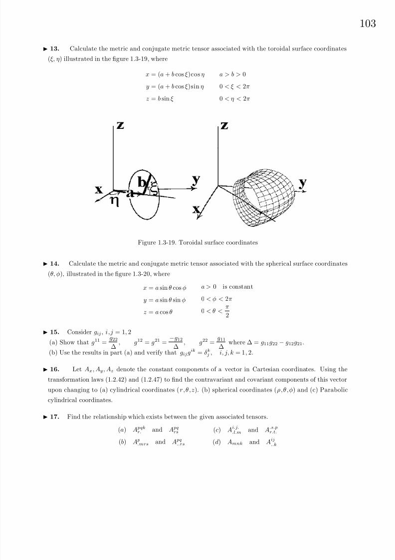
8/6/2019 Introduction to Tensor Calculus Continuum Mechanics - J. Heinbockel
http://slidepdf.com/reader/full/introduction-to-tensor-calculus-continuum-mechanics-j-heinbockel 108/372
10
13. Calculate the metric and conjugate metric tensor associated with the toroidal surface coordinates
(ξ, η) illustrated in the figure 1.3-19, where
x = (a + b cos ξ)cos η
y = (a + b cos ξ)sin η
z = b sin ξ
a > b > 0
0 < ξ < 2π
0 < η < 2π
Figure 1.3-19. Toroidal surface coordinates
14. Calculate the metric and conjugate metric tensor associated with the spherical surface coordinates
(θ, φ), illustrated in the figure 1.3-20, where
x = a sin θ cos φ
y = a sin θ sin φ
z = a cos θ
a > 0 is constant
0 < φ < 2π
0 < θ <π
2
15. Consider gij , i,j = 1, 2
(a) Show that g11 =g22∆
, g12 = g21 =−g12
∆, g22 =
g11∆
where ∆ = g11g22 − g12g21.
(b) Use the results in part (a) and verify that gijgik = δkj , i, j, k = 1, 2.
16. Let Ax, Ay, Az denote the constant components of a vector in Cartesian coordinates. Using the
transformation laws (1.2.42) and (1.2.47) to find the contravariant and covariant components of this vector
upon changing to (a) cylindrical coordinates (r,θ,z). (b) spherical coordinates (ρ,θ,φ) and (c) Paraboliccylindrical coordinates.
17. Find the relationship which exists between the given associated tensors.
(a) A pqkr. and A pq
rs
(b) A p.mrs and A pq
..rs
(c) Ai.j..l.m and A.s.p
r.t.
(d) Amnk and Aij..k
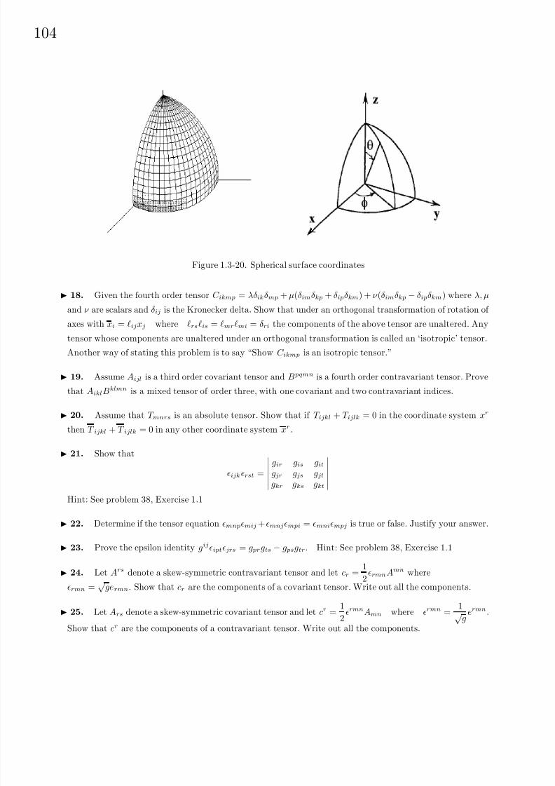
8/6/2019 Introduction to Tensor Calculus Continuum Mechanics - J. Heinbockel
http://slidepdf.com/reader/full/introduction-to-tensor-calculus-continuum-mechanics-j-heinbockel 109/372
104
Figure 1.3-20. Spherical surface coordinates
18. Given the fourth order tensor C ikmp = λδikδmp + µ(δimδkp + δipδkm) + ν (δimδkp − δipδkm) where λ, µ
and ν are scalars and δij is the Kronecker delta. Show that under an orthogonal transformation of rotation of
axes with xi = ijxj where rsis = mrmi = δri the components of the above tensor are unaltered. Any
tensor whose components are unaltered under an orthogonal transformation is called an ‘isotropic’ tensor.
Another way of stating this problem is to say “Show C ikmp is an isotropic tensor.”
19. Assume Aijl is a third order covariant tensor and B pqmn is a fourth order contravariant tensor. Prove
that AiklBklmn is a mixed tensor of order three, with one covariant and two contravariant indices.
20. Assume that T mnrs is an absolute tensor. Show that if T ijkl + T ijlk = 0 in the coordinate system xr
then T ijkl + T ijlk = 0 in any other coordinate system xr.
21. Show that
ijkrst =
gir gis gitgjr gjs gjtgkr gks gkt
Hint: See problem 38, Exercise 1.1
22. Determine if the tensor equation mnpmij + mnjmpi = mnimpj is true or false. Justify your answer.
23. Prove the epsilon identity gij
iptjrs = g prgts − g psgtr. Hint: See problem 38, Exercise 1.1
24. Let Ars denote a skew-symmetric contravariant tensor and let cr =1
2rmnAmn where
rmn =√
germn. Show that cr are the components of a covariant tensor. Write out all the components.
25. Let Ars denote a skew-symmetric covariant tensor and let cr =1
2rmnAmn where rmn =
1√g
ermn.
Show that cr are the components of a contravariant tensor. Write out all the components.
8/6/2019 Introduction to Tensor Calculus Continuum Mechanics - J. Heinbockel
http://slidepdf.com/reader/full/introduction-to-tensor-calculus-continuum-mechanics-j-heinbockel 110/372
10
26. Let A pqBqsr = C s pr where Bqs
r is a relative tensor of weight ω1 and C s pr is a relative tensor of weight
ω2. Prove that A pq is a relative tensor of weight (ω2 − ω1).
27. When Aij is an absolute tensor prove that
√gAi
j is a relative tensor of weight +1.
28. When A
i
j is an absolute tensor prove that
1
√ gA
i
j is a relative tensor of weight −1.
29.
(a) Show eijk is a relative tensor of weight +1.
(b) Show ijk = 1√ g
eijk is an absolute tensor. Hint: See example 1.1-25.
30. The equation of a surface can be represented by an equation of the form Φ(x1, x2, x3) = constant.
Show that a unit normal vector to the surface can be represented by the vector
ni =gij ∂ Φ
∂xj
(gmn ∂ Φ∂xm
∂ Φ∂xn
)1
2
.
31. Assume that gij = λgij with λ a nonzero constant. Find and calculate gij in terms of gij.
32. Determine if the following tensor equation is true. Justify your answer.
rjkAri + irkAr
j + ijrArk = ijkAr
r.
Hint: See problem 21, Exercise 1.1.
33. Show that for C i and C i associated tensors, and C i = ijkAjBk, then C i = ijkAjBk
34. Prove that ijk and ijk are associated tensors. Hint: Consider the determinant of gij .
35. Show ijkAiBjC k = ijkAiBjC k.
36. Let T ij , i, j = 1, 2, 3 denote a second order mixed tensor. Show that the given quantities are scalar
invariants.(i) I 1 = T ii
(ii) I 2 =1
2
(T ii )2 − T imT mi
(iii) I 3 = det|T ij |
37.
(a) Assume Aij
and Bij
, i, j = 1, 2, 3 are absolute contravariant tensors, and determine if the inner productC ik = AijBjk is an absolute tensor?
(b) Assume that the condition∂xj
∂xn
∂xj
∂xm= δnm is satisfied, and determine whether the inner product in
part (a) is a tensor?
(c) Consider only transformations which are a rotation and translation of axes yi = ijyj + bi, where ij are
direction cosines for the rotation of axes. Show that∂yj
∂yn
∂yj
∂ym= δnm

8/6/2019 Introduction to Tensor Calculus Continuum Mechanics - J. Heinbockel
http://slidepdf.com/reader/full/introduction-to-tensor-calculus-continuum-mechanics-j-heinbockel 111/372
106
38. For Aijk a Cartesian tensor, determine if a contraction on the indices i and j is allowed. That
is, determine if the quantity Ak = Aiik, (summation on i) is a tensor. Hint: See part(c) of the previous
problem.
39. Prove the e-δ identity eijkeimn = δjmδkn − δjnδkm.
40. Consider the vector V k, k = 1, 2, 3 and define the matrix (aij) having the elements aij = eijkV k,
where eijk is the e−permutation symbol.
(a) Solve for V i in terms of amn by multiplying both sides of the given equation by eijl and note the e − δ
identity allows us to simplify the result.
(b) Sum the given expression on k and then assign values to the free indices (i,j=1,2,3) and compare your
results with part (a).
(c) Is aij symmetric, skew-symmetric, or neither?
41. It can be shown that the continuity equation of fluid dynamics can be expressed in the tensor form
1√g
∂
∂xr (√gV r) +∂
∂t = 0,
where is the density of the fluid, t is time, V r, with r = 1, 2, 3 are the velocity components and g = |gij |is the determinant of the metric tensor. Employing the summation convention and replacing the tensor
components of velocity by their physical components, express the continuity equation in
(a) Cartesian coordinates (x, y, z) with physical components V x, V y, V z.
(b) Cylindrical coordinates (r,θ,z) with physical components V r, V θ, V z.
(c) Spherical coordinates (ρ,θ,φ) with physical components V ρ, V θ, V φ.
42. Let x1, x2, x3 denote a set of skewed coordinates with respect to the Cartesian coordinates y1, y2, y3.
Assume that E 1, E 2, E 3 are unit vectors in the directions of the x1, x2 and x3 axes respectively. If the unit
vectors satisfy the relations E 1 · E 1 = 1
E 2 · E 2 = 1
E 3 · E 3 = 1
E 1 · E 2 = cos θ12
E 1 · E 3 = cos θ13
E 2 · E 3 = cos θ23,
then calculate the metrices gij and conjugate metrices gij.
43. Let Aij , i, j = 1, 2, 3, 4 denote the skew-symmetric second rank tensor
Aij =
0 a b c−a 0 d e−b −d 0 f −c −e −f 0
,
where a,b,c,d,e,f are complex constants. Calculate the components of the dual tensor
V ij =1
2eijklAkl.

8/6/2019 Introduction to Tensor Calculus Continuum Mechanics - J. Heinbockel
http://slidepdf.com/reader/full/introduction-to-tensor-calculus-continuum-mechanics-j-heinbockel 112/372
10
44. In Cartesian coordinates the vorticity tensor at a point in a fluid medium is defined
ωij =1
2
∂V j∂xi
− ∂V i∂xj
where V i are the velocity components of the fluid at the point. The vorticity vector at a point in a fluid
medium in Cartesian coordinates is defined by ωi =1
2eijkωjk . Show that these tensors are dual tensors.
45. Write out the relation between each of the components of the dual tensors
T ij =1
2eijklT kl i, j, k, l = 1, 2, 3, 4
and show that if ijkl is an even permutation of 1234, then T ij = T kl.
46. Consider the general affine transformation xi = aijxj where (x1, x2, x3) = (x, y, z) with inverse
transformation xi = bij xj . Determine (a) the image of the plane Ax + By + Cz + D = 0 under this
transformation and (b) the image of a second degree conic section
Ax2 + 2Bxy + Cy2 + Dx + Ey + F = 0.
47. Using a multilinear form of degree M, derive the transformation law for a contravariant vector of
degree M.
48. Let g denote the determinant of gij and show that∂g
∂xk= ggij ∂gij
∂xk.
49. We have shown that for a rotation of xyz axes with respect to a set of fixed xyz axes, the derivative
of a vector A with respect to an observer on the barred axes is given by
d A
dt
f
=d A
dt
r
+ ω × A.
Introduce the operators
Df A =
d A
dt f = derivative in fixed system
Dr A =
d A
dt
r
= derivative in rotating system
(a) Show that Df A = (Dr + ω×) A.
(b) Consider the special case that the vector A is the position vector r. Show that Df r = (Dr + ω×)r
produces V
f
= V
r
+ ω × r where V
f
represents the velocity of a particle relative to the fixed system
and V
r
represents the velocity of a particle with respect to the rotating system of coordinates.
(c) Show that af = ar + ω × ( ω × r) where af represents the acceleration of a particle relative to the
fixed system and ar
represents the acceleration of a particle with respect to the rotating system.
(d) Show in the special case ω is a constant that
a
f
= 2 ω × V + ω × ( ω × r)
where V is the velocity of the particle relative to the rotating system. The term 2 ω × V is referred to
as the Coriolis acceleration and the term ω × ( ω × r) is referred to as the centripetal acceleration.
8/6/2019 Introduction to Tensor Calculus Continuum Mechanics - J. Heinbockel
http://slidepdf.com/reader/full/introduction-to-tensor-calculus-continuum-mechanics-j-heinbockel 113/372
108
§1.4 DERIVATIVE OF A TENSOR
In this section we develop some additional operations associated with tensors. Historically, one of the
basic problems of the tensor calculus was to try and find a tensor quantity which is a function of the metric
tensor gij and some of its derivatives∂gij
∂xm,
∂ 2gij
∂xm∂xn, . . . . A solution of this problem is the fourth order
Riemann Christoffel tensor Rijkl to be developed shortly. In order to understand how this tensor was arrivedat, we must first develop some preliminary relationships involving Christoffel symbols.
Christoffel Symbols
Let us consider the metric tensor gij which we know satisfies the transformation law
gαβ = gab∂xa
∂xα
∂xb
∂xβ.
Define the quantity
(α ,β ,γ ) =
∂g αβ
∂xγ =∂gab
∂xc
∂xc
∂xγ
∂xa
∂xα
∂xb
∂xβ + gab
∂ 2xa
∂xα∂xγ
∂xb
∂xβ + gab
∂xa
∂xα
∂ 2xb
∂xβ∂xγ
and form the combination of terms1
2[(α ,β ,γ ) + (β , γ , α) − (γ , α , β )] to obtain the result
1
2
∂g αβ
∂xγ +∂g βγ
∂xα − ∂g γα
∂xβ
=
1
2
∂gab
∂xc+
∂gbc
∂xa− ∂gca
∂xb
∂xa
∂xα
∂xb
∂xβ
∂xc
∂xγ + gab∂xb
∂xβ
∂ 2xa
∂xα∂xγ . (1.4.1)
In this equation the combination of derivatives occurring inside the brackets is called a Christoffel symbol
of the first kind and is defined by the notation
[ac,b] = [ca,b] =1
2∂gab
∂xc
+∂gbc
∂xa
−∂gac
∂xb . (1.4.2)
The equation (1.4.1) defines the transformation for a Christoffel symbol of the first kind and can be expressed
as
[α γ , β ] = [ac,b]∂xa
∂xα
∂xb
∂xβ
∂xc
∂xγ + gab∂ 2xa
∂xα∂xγ
∂xb
∂xβ. (1.4.3)
Observe that the Christoffel symbol of the first kind [ac,b] does not transform like a tensor. However, it is
symmetric in the indices a and c.
At this time it is convenient to use the equation (1.4.3) to develop an expression for the second derivative
term which occurs in that equation as this second derivative term arises in some of our future considerations.
To solve for this second derivative we can multiply equation (1.4.3) by∂xβ
∂x
dgde and simplify the result to the
form∂ 2xe
∂xα∂xγ = −gde[ac,d]∂xa
∂xα
∂xc
∂xγ + [α γ , β ]∂xβ
∂xdgde. (1.4.4)
The transformation gde = gλµ ∂xd
∂xλ
∂xe
∂xµ allows us to express the equation (1.4.4) in the form
∂ 2xe
∂xα∂xγ = −gde[ac,d]∂xa
∂xα
∂xc
∂xγ + gβµ[α γ , β ]∂xe
∂xµ . (1.4.5)

8/6/2019 Introduction to Tensor Calculus Continuum Mechanics - J. Heinbockel
http://slidepdf.com/reader/full/introduction-to-tensor-calculus-continuum-mechanics-j-heinbockel 114/372
10
Define the Christoffel symbol of the second kind as
i
j k
=
i
k j
= giα[ jk,α] =
1
2giα
∂gkα
∂xj+
∂gjα
∂xk− ∂gjk
∂xα
. (1.4.6)
This Christoffel symbol of the second kind is symmetric in the indices j and k and from equation (1.4.5) we
see that it satisfies the transformation lawµ
α γ
∂xe
∂xµ =
e
a c
∂xa
∂xα
∂xc
∂xγ +∂ 2xe
∂xα∂xγ . (1.4.7)
Observe that the Christoffel symbol of the second kind does not transform like a tensor quantity. We can use
the relation defined by equation (1.4.7) to express the second derivative of the transformation equations in
terms of the Christoffel symbols of the second kind. At times it will be convenient to represent the Christoffel
symbols with a subscript to indicate the metric from which they are calculated. Thus, an alternative notation
for
i
j k
is the notation
i
j k
g
.
EXAMPLE 1.4-1. (Christoffel symbols) Solve for the Christoffel symbol of the first kind in terms of the Christoffel symbol of the second kind.
Solution: By the definition from equation (1.4.6) we have
i
j k
= giα[ jk,α].
We multiply this equation by gβi and find
gβi
i
j k
= δα
β [ jk,α] = [ jk,β ]
and so[ jk,α] = gαi
i
j k
= gα1
1
j k
+ · · · + gαN
N
j k
.
EXAMPLE 1.4-2. (Christoffel symbols of first kind)
Derive formulas to find the Christoffel symbols of the first kind in a generalized orthogonal coordinate
system with metric coefficients
gij = 0 for i = j and g(i)(i) = h2(i), i = 1, 2, 3
where i is not summed.Solution: In an orthogonal coordinate system where gij = 0 for i = j we observe that
[ab,c] =1
2
∂gac
∂xb+
∂gbc
∂xa− ∂gab
∂xc
. (1.4.8)
Here there are 33 = 27 quantities to calculate. We consider the following cases:

8/6/2019 Introduction to Tensor Calculus Continuum Mechanics - J. Heinbockel
http://slidepdf.com/reader/full/introduction-to-tensor-calculus-continuum-mechanics-j-heinbockel 115/372

8/6/2019 Introduction to Tensor Calculus Continuum Mechanics - J. Heinbockel
http://slidepdf.com/reader/full/introduction-to-tensor-calculus-continuum-mechanics-j-heinbockel 116/372
11
EXAMPLE 1.4-4. (Christoffel symbols of the second kind)
Find formulas for the calculation of the Christoffel symbols of the second kind in a generalized orthogonal
coordinate system with metric coefficients
gij = 0 for i = j and g(i)(i) = h2(i), i = 1, 2, 3
where i is not summed.
Solution: By definition we have
i
j k
= gim[ jk,m] = gi1[ jk, 1] + gi2[ jk, 2] + gi3[ jk, 3] (1.4.12)
By hypothesis the coordinate system is orthogonal and so
gij = 0 for i = j and gii =1
giii not summed.
The only nonzero term in the equation (1.4.12) occurs when m = i and consequently
i
j k
= gii[ jk,i] =
[ jk,i]
giino summation on i. (1.4.13)
We can now consider the four cases considered in the example 1.4-2.
CASE I Let j = k = i and show
i
i i
=
[ii,i]
gii=
1
2gii
∂gii
∂xi=
1
2
∂
∂xiln gii no summation on i. (1.4.14)
CASE II Let k = j = i and show
i
j j
= [ jj,i]
gii= −1
2gii
∂gjj
∂xino summation on i or j. (1.4.15)
CASE III Let i = j = k and verify that
j
j k
=
j
k j
=
[ jk,j]
gjj=
1
2gjj
∂gjj
∂xk=
1
2
∂
∂xkln gjj no summation on i or j. (1.4.16)
CASE IV For the case i = j = k we find
i
j k
=
[ jk,i]
gii= 0, i = j = k no summation on i.
The above cases represent all 27 terms.
8/6/2019 Introduction to Tensor Calculus Continuum Mechanics - J. Heinbockel
http://slidepdf.com/reader/full/introduction-to-tensor-calculus-continuum-mechanics-j-heinbockel 117/372
112
EXAMPLE 1.4-5. (Notation) In the case of cylindrical coordinates we can use the above relations and
find the nonzero Christoffel symbols of the second kind:1
2 2
= − 1
2g11
∂g22
∂x1= −x1 = −r
2
1 2
= 2
2 1
=1
2g22
∂g22
∂x1 =1
x1 =1
r
Note 1: The notation for the above Christoffel symbols are based upon the assumption that x1 = r, x2 = θ
and x3 = z. However, in tensor calculus the choice of the coordinates can be arbitrary. We could just as well
have defined x1 = z, x2 = r and x3 = θ. In this latter case, the numbering system of the Christoffel symbols
changes. To avoid confusion, an alternate method of writing the Christoffel symbols is to use coordinates in
place of the integers 1,2 and 3. For example, in cylindrical coordinates we can writeθ
r θ
=
θ
θ r
=
1
rand
r
θ θ
= −r.
If we define x1
= r, x2
= θ, x3
= z, then the nonzero Christoffel symbols are written as2
1 2
=
2
2 1
=
1
rand
1
2 2
= −r.
In contrast, if we define x1 = z, x2 = r, x3 = θ, then the nonzero Christoffel symbols are written3
2 3
=
3
3 2
=
1
rand
2
3 3
= −r.
Note 2: Some textbooks use the notation Γa,bc for Christoffel symbols of the first kind and Γdbc = gdaΓa,bc for
Christoffel symbols of the second kind. This notation is not used in these notes since the notation suggests
that the Christoffel symbols are third order tensors, which is not true. The Christoffel symbols of the first
and second kind are not tensors. This fact is clearly illustrated by the transformation equations (1.4.3) and
(1.4.7).
Covariant Differentiation
Let Ai denote a covariant tensor of rank 1 which obeys the transformation law
Aα = Ai∂xi
∂xα . (1.4.17)
Differentiate this relation with respect to xβ and show
∂Aα
∂xβ= Ai
∂ 2xi
∂xα∂xβ+
∂Ai
∂xj
∂xj
∂xβ
∂xi
∂xα . (1.4.18)
Now use the relation from equation (1.4.7) to eliminate the second derivative term from (1.4.18) and express
it in the form∂Aα
∂xβ= Ai
σ
α β
∂xi
∂xσ −
i
j k
∂xj
∂xα
∂xk
∂xβ
+
∂Ai
∂xj
∂xj
∂xβ
∂xi
∂xα . (1.4.19)
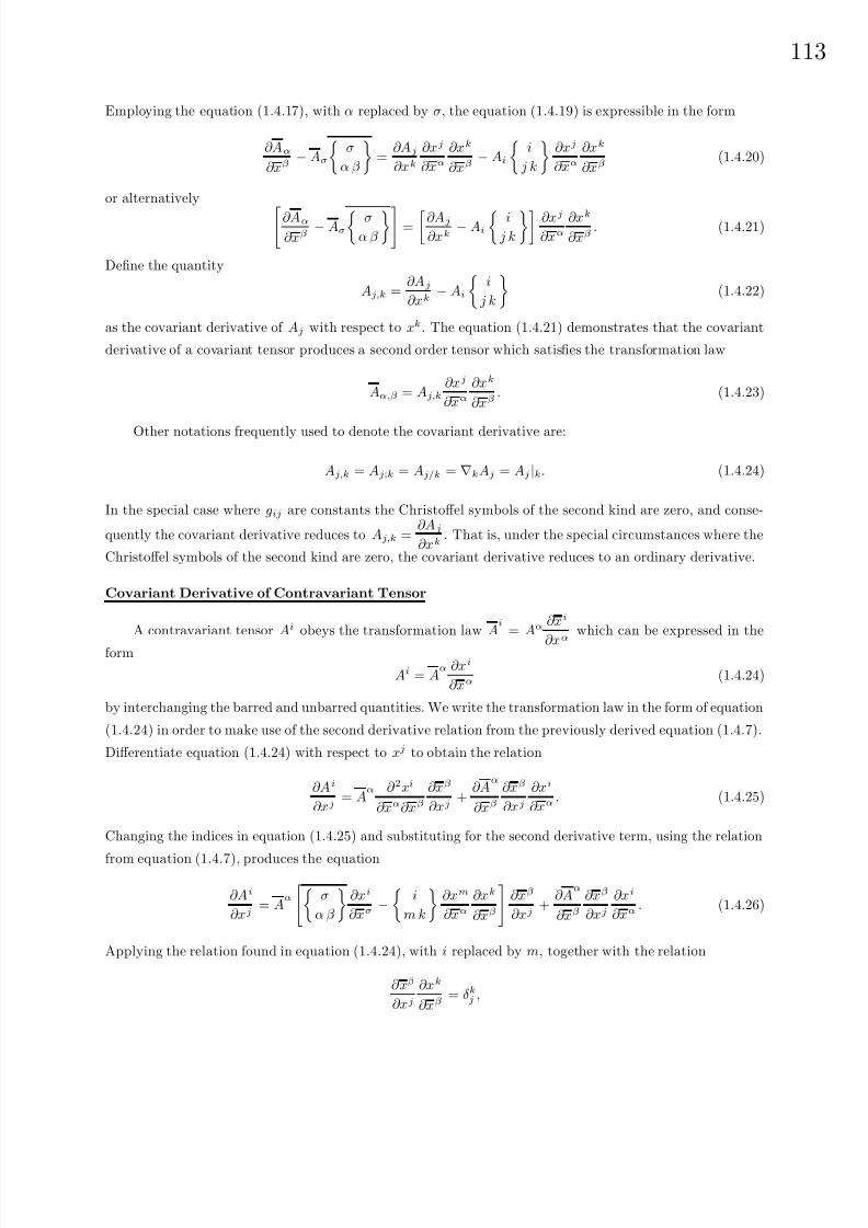
8/6/2019 Introduction to Tensor Calculus Continuum Mechanics - J. Heinbockel
http://slidepdf.com/reader/full/introduction-to-tensor-calculus-continuum-mechanics-j-heinbockel 118/372
11
Employing the equation (1.4.17), with α replaced by σ, the equation (1.4.19) is expressible in the form
∂Aα
∂xβ− Aσ
σ
α β
=
∂Aj
∂xk
∂xj
∂xα
∂xk
∂xβ− Ai
i
j k
∂xj
∂xα
∂xk
∂xβ(1.4.20)
or alternatively ∂Aα
∂xβ− Aσ
σ
α β
=
∂Aj
∂xk− Ai
i
j k
∂xj
∂xα∂xk
∂xβ. (1.4.21)
Define the quantity
Aj,k =∂Aj
∂xk− Ai
i
j k
(1.4.22)
as the covariant derivative of Aj with respect to xk. The equation (1.4.21) demonstrates that the covariant
derivative of a covariant tensor produces a second order tensor which satisfies the transformation law
Aα,β = Aj,k∂xj
∂xα
∂xk
∂xβ. (1.4.23)
Other notations frequently used to denote the covariant derivative are:
Aj,k = Aj;k = Aj/k = ∇kAj = Aj |k. (1.4.24)
In the special case where gij are constants the Christoffel symbols of the second kind are zero, and conse-
quently the covariant derivative reduces to Aj,k =∂Aj
∂xk. That is, under the special circumstances where the
Christoffel symbols of the second kind are zero, the covariant derivative reduces to an ordinary derivative.
Covariant Derivative of Contravariant Tensor
A contravariant tensor Ai obeys the transformation law Ai
= Aα ∂xi
∂xα
which can be expressed in the
form
Ai = Aα ∂xi
∂xα (1.4.24)
by interchanging the barred and unbarred quantities. We write the transformation law in the form of equation
(1.4.24) in order to make use of the second derivative relation from the previously derived equation (1.4.7).
Differentiate equation (1.4.24) with respect to xj to obtain the relation
∂Ai
∂xj= A
α ∂ 2xi
∂xα∂xβ
∂xβ
∂xj+
∂Aα
∂xβ
∂xβ
∂xj
∂xi
∂xα . (1.4.25)
Changing the indices in equation (1.4.25) and substituting for the second derivative term, using the relation
from equation (1.4.7), produces the equation
∂Ai
∂xj= A
α
σ
α β
∂xi
∂xσ −
i
m k
∂xm
∂xα
∂xk
∂xβ
∂xβ
∂xj+
∂Aα
∂xβ
∂xβ
∂xj
∂xi
∂xα . (1.4.26)
Applying the relation found in equation (1.4.24), with i replaced by m, together with the relation
∂ xβ
∂xj
∂xk
∂xβ= δk
j ,

8/6/2019 Introduction to Tensor Calculus Continuum Mechanics - J. Heinbockel
http://slidepdf.com/reader/full/introduction-to-tensor-calculus-continuum-mechanics-j-heinbockel 119/372
114
we simplify equation (1.4.26) to the form
∂Ai
∂xj+
i
m j
Am
=
∂A
σ
∂xβ+
σ
α β
A
α
∂xβ
∂xj
∂xi
∂xσ . (1.4.27)
Define the quantity
Ai,j =
∂Ai
∂xj+
i
m j
Am (1.4.28)
as the covariant derivative of the contravariant tensor Ai. The equation (1.4.27) demonstrates that a covariant
derivative of a contravariant tensor will transform like a mixed second order tensor and
Ai,j = A
σ,β
∂xβ
∂xj
∂xi
∂xσ . (1.4.29)
Again it should be observed that for the condition where gij are constants we have Ai,j =
∂Ai
∂xjand the
covariant derivative of a contravariant tensor reduces to an ordinary derivative in this special case.
In a similar manner the covariant derivative of second rank tensors can be derived. We find these
derivatives have the forms:
Aij,k =∂Aij
∂xk− Aσj
σ
i k
− Aiσ
σ
j k
Aij ,k =
∂Aij
∂xk+ Aσ
j
i
σ k
− Ai
σ
σ
j k
Aij
,k =∂Aij
∂xk+ Aσj
i
σ k
+ Aiσ
j
σ k
.
(1.4.30)
In general, the covariant derivative of a mixed tensor
Aij...klm...p
of rank n has the form
Aij...klm...p,q =
∂Aij...klm...p
∂xq+ Aσj...k
lm...p
i
σ q
+ Aiσ...k
lm...p
j
σ q
+ · · · + Aij...σ
lm...p
k
σ q
− Aij...kσm...p
σ
l q
− Aij...k
lσ...p
σ
m q
− · · · −Aij...k
lm...σ
σ
p q
(1.4.31)
and this derivative is a tensor of rank n + 1. Note the pattern of the + signs for the contravariant indices
and the − signs for the covariant indices.
Observe that the covariant derivative of an nth order tensor produces an n+1st order tensor, the indices
of these higher order tensors can also be raised and lowered by multiplication by the metric or conjugate
metric tensor. For example we can write
gimAjk |m = Ajk |i and gimAjk |m = Ajk |i
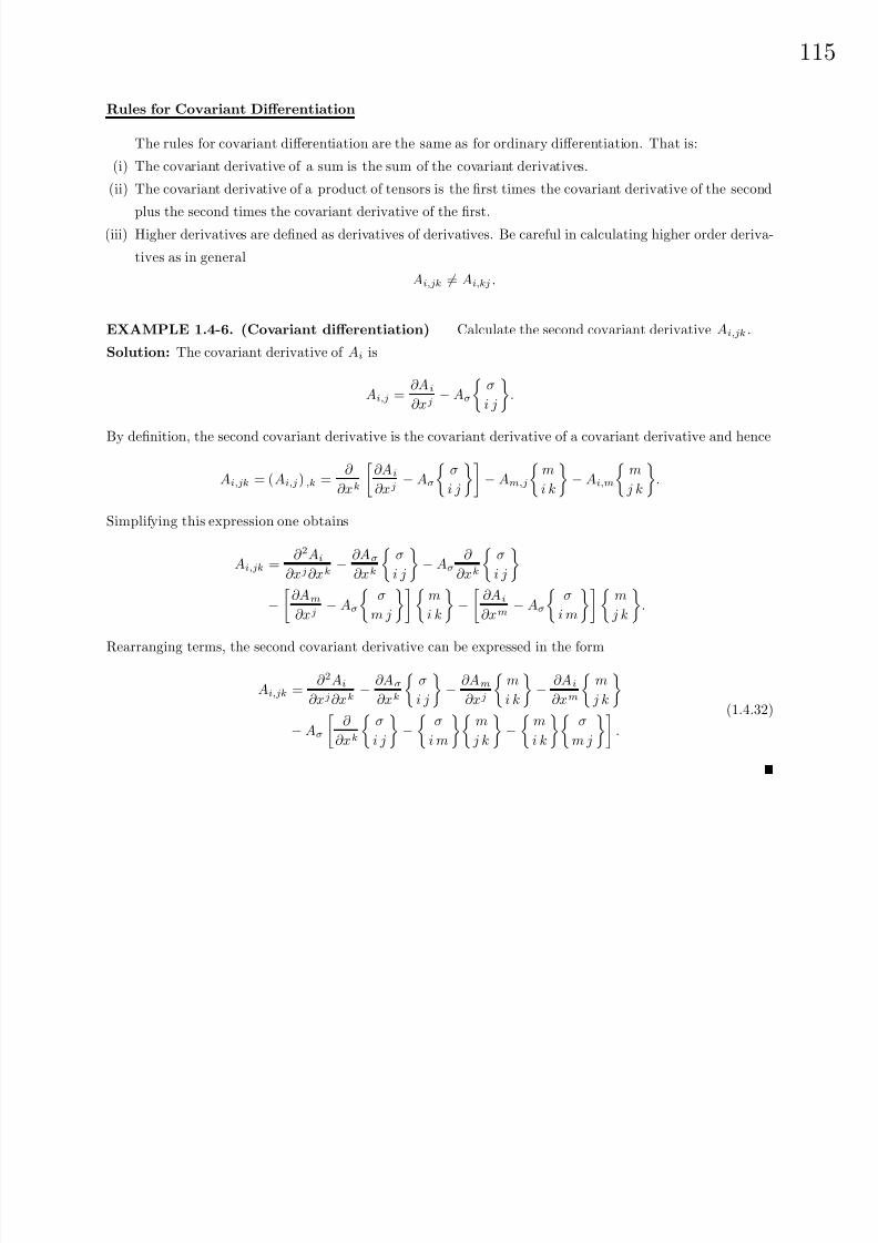
8/6/2019 Introduction to Tensor Calculus Continuum Mechanics - J. Heinbockel
http://slidepdf.com/reader/full/introduction-to-tensor-calculus-continuum-mechanics-j-heinbockel 120/372
11
Rules for Covariant Differentiation
The rules for covariant differentiation are the same as for ordinary differentiation. That is:
(i) The covariant derivative of a sum is the sum of the covariant derivatives.
(ii) The covariant derivative of a product of tensors is the first times the covariant derivative of the second
plus the second times the covariant derivative of the first.(iii) Higher derivatives are defined as derivatives of derivatives. Be careful in calculating higher order deriva-
tives as in general
Ai,jk = Ai,kj .
EXAMPLE 1.4-6. (Covariant differentiation) Calculate the second covariant derivative Ai,jk .
Solution: The covariant derivative of Ai is
Ai,j =∂Ai
∂xj− Aσ
σ
i j
.
By definition, the second covariant derivative is the covariant derivative of a covariant derivative and hence
Ai,jk = (Ai,j ) ,k =∂
∂xk
∂Ai
∂xj− Aσ
σ
i j
− Am,j
m
i k
− Ai,m
m
j k
.
Simplifying this expression one obtains
Ai,jk =∂ 2Ai
∂xj ∂xk− ∂Aσ
∂xk
σ
i j
− Aσ
∂
∂xk
σ
i j
−
∂Am
∂xj− Aσ
σ
m j
m
i k
−
∂Ai
∂xm− Aσ
σ
i m
m
j k
.
Rearranging terms, the second covariant derivative can be expressed in the form
Ai,jk =∂ 2Ai
∂xj ∂xk− ∂Aσ
∂xk
σ
i j
− ∂Am
∂xj
m
i k
− ∂Ai
∂xm
m
j k
− Aσ
∂
∂xk
σ
i j
−
σ
i m
m
j k
−
m
i k
σ
m j
.
(1.4.32)
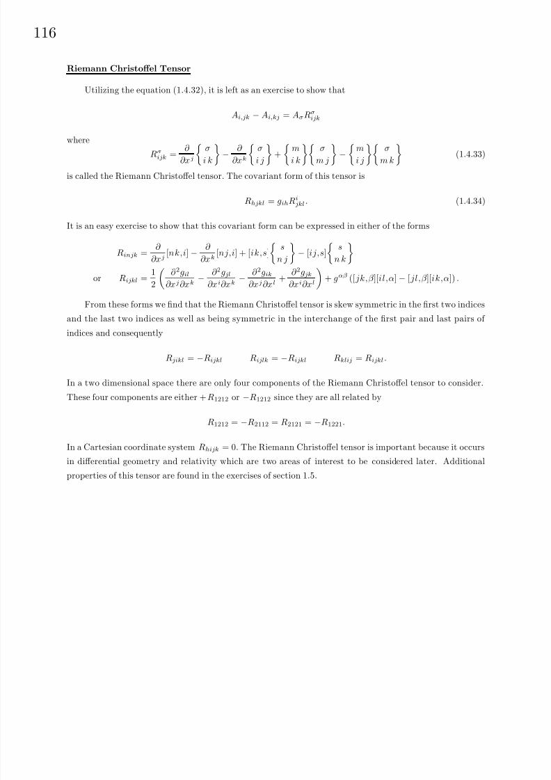
8/6/2019 Introduction to Tensor Calculus Continuum Mechanics - J. Heinbockel
http://slidepdf.com/reader/full/introduction-to-tensor-calculus-continuum-mechanics-j-heinbockel 121/372
116
Riemann Christoffel Tensor
Utilizing the equation (1.4.32), it is left as an exercise to show that
Ai,jk − Ai,kj = AσRσijk
where
Rσijk =
∂
∂xj
σ
i k
− ∂
∂xk
σ
i j
+
m
i k
σ
m j
−
m
i j
σ
m k
(1.4.33)
is called the Riemann Christoffel tensor. The covariant form of this tensor is
Rhjkl = gihRijkl . (1.4.34)
It is an easy exercise to show that this covariant form can be expressed in either of the forms
Rinjk =∂
∂xj[nk,i] − ∂
∂xk[nj,i] + [ik,s]
s
n j
− [ij,s]
s
n k
or Rijkl = 12
∂ 2
gil
∂xj ∂xk− ∂
2
gjl
∂xi∂xk− ∂
2
gik
∂xj ∂xl+ ∂
2
gjk
∂xi∂xl
+ gαβ ([ jk,β ][il,α] − [ jl,β ][ik,α]) .
From these forms we find that the Riemann Christoffel tensor is skew symmetric in the first two indices
and the last two indices as well as being symmetric in the interchange of the first pair and last pairs of
indices and consequently
Rjikl = −Rijkl Rijlk = −Rijkl Rklij = Rijkl .
In a two dimensional space there are only four components of the Riemann Christoffel tensor to consider.
These four components are either +R1212 or −R1212 since they are all related by
R1212 = −R2112 = R2121 = −R1221.
In a Cartesian coordinate system Rhijk = 0. The Riemann Christoffel tensor is important because it occurs
in differential geometry and relativity which are two areas of interest to be considered later. Additional
properties of this tensor are found in the exercises of section 1.5.
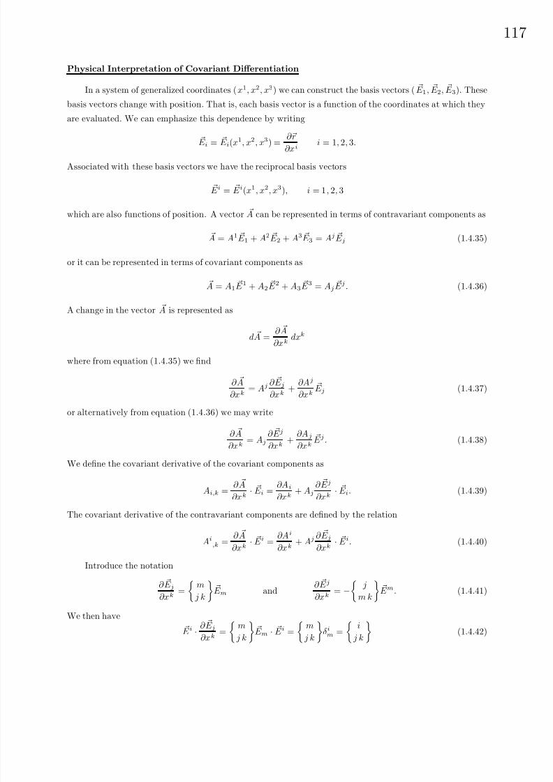
8/6/2019 Introduction to Tensor Calculus Continuum Mechanics - J. Heinbockel
http://slidepdf.com/reader/full/introduction-to-tensor-calculus-continuum-mechanics-j-heinbockel 122/372
11
Physical Interpretation of Covariant Differentiation
In a system of generalized coordinates (x1, x2, x3) we can construct the basis vectors ( E 1, E 2, E 3). These
basis vectors change with position. That is, each basis vector is a function of the coordinates at which they
are evaluated. We can emphasize this dependence by writing
E i = E i(x1, x2, x3) = ∂r∂xi
i = 1, 2, 3.
Associated with these basis vectors we have the reciprocal basis vectors
E i = E i(x1, x2, x3), i = 1, 2, 3
which are also functions of position. A vector A can be represented in terms of contravariant components as
A = A1 E 1 + A2 E 2 + A3 E 3 = Aj E j (1.4.35)
or it can be represented in terms of covariant components as
A = A1 E 1 + A2
E 2 + A3 E 3 = Aj
E j . (1.4.36)
A change in the vector A is represented as
d A =∂ A
∂xkdxk
where from equation (1.4.35) we find
∂ A
∂xk= Aj ∂ E j
∂xk+
∂Aj
∂xk E j (1.4.37)
or alternatively from equation (1.4.36) we may write
∂ A
∂xk= Aj
∂ E j
∂xk+
∂Aj
∂xk E j . (1.4.38)
We define the covariant derivative of the covariant components as
Ai,k =∂ A
∂xk· E i =
∂Ai
∂xk+ Aj
∂ E j
∂xk· E i. (1.4.39)
The covariant derivative of the contravariant components are defined by the relation
Ai
,k
=∂ A
∂xk · E i =
∂Ai
∂xk
+ Aj ∂ E j
∂xk · E i. (1.4.40)
Introduce the notation
∂ E j
∂xk=
m
j k
E m and
∂ E j
∂xk= −
j
m k
E m. (1.4.41)
We then have
E i · ∂ E j
∂xk=
m
j k
E m · E i =
m
j k
δi
m =
i
j k
(1.4.42)

8/6/2019 Introduction to Tensor Calculus Continuum Mechanics - J. Heinbockel
http://slidepdf.com/reader/full/introduction-to-tensor-calculus-continuum-mechanics-j-heinbockel 123/372
118
and
E i · ∂ E j
∂xk= −
j
m k
E m · E i = −
j
m k
δm
i = −
j
i k
. (1.4.43)
Then equations (1.4.39) and (1.4.40) become
Ai,k =
∂Ai
∂xk − j
i k
Aj
Ai,k =
∂Ai
∂xk+
i
j k
Aj ,
which is consistent with our earlier definitions from equations (1.4.22) and (1.4.28). Here the first term of
the covariant derivative represents the rate of change of the tensor field as we move along a coordinate curve.
The second term in the covariant derivative represents the change in the local basis vectors as we move
along the coordinate curves. This is the physical interpretation associated with the Christoffel symbols of
the second kind.
We make the observation that the derivatives of the basis vectors in equations (1.4.39) and (1.4.40) are
related since E i · E j = δ
ji
and consequently∂
∂xk( E i · E j ) = E i · ∂ E j
∂xk+
∂ E i
∂xk· E j = 0
or E i · ∂ E j
∂xk= − E j · ∂ E i
∂xk
Hence we can express equation (1.4.39) in the form
Ai,k =∂Ai
∂xk− Aj
E j · ∂ E i
∂xk. (1.4.44)
We write the first equation in (1.4.41) in the form
∂ E j
∂xk=
m
j k
gim
E i = [ jk,i] E i (1.4.45)
and consequently∂ E j
∂xk· E m =
i
j k
E i · E m =
i
j k
δm
i =
m
j k
and∂ E j
∂xk· E m =[ jk,i] E i · E m = [ jk,i]δi
m = [ jk,m].
(1.4.46)
These results also reduce the equations (1.4.40) and (1.4.44) to our previous forms for the covariant deriva-
tives.The equations (1.4.41) are representations of the vectors ∂ Ei
∂xkand ∂ Ej
∂xkin terms of the basis vectors and
reciprocal basis vectors of the space. The covariant derivative relations then take into account how these
vectors change with position and affect changes in the tensor field.
The Christoffel symbols in equations (1.4.46) are symmetric in the indices j and k since
∂ E j
∂xk=
∂
∂xk
∂r
∂xj
=
∂
∂xj
∂r
∂xk
=
∂ E k
∂xj. (1.4.47)

8/6/2019 Introduction to Tensor Calculus Continuum Mechanics - J. Heinbockel
http://slidepdf.com/reader/full/introduction-to-tensor-calculus-continuum-mechanics-j-heinbockel 124/372
11
The equations (1.4.46) and (1.4.47) enable us to write
[ jk,m] = E m · ∂ E j
∂xk=
1
2
E m · ∂ E j
∂xk+ E m · ∂ E k
∂xj
=1
2 ∂
∂xk E m
· E j +
∂
∂xj E m
· E k−
E j
·
∂ E m
∂xk
− E k
·
∂ E m
∂xj
=1
2
∂
∂xk
E m · E j
+
∂
∂xj
E m · E k
− E j · ∂ E k
∂xm− E k · ∂ E j
∂xm
=1
2
∂
∂xk
E m · E j
+
∂
∂xj
E m · E k
− ∂
∂xm
E j · E k
=1
2
∂gmj
∂xk+
∂gmk
∂xj− ∂gjk
∂xm
= [kj,m]
which again agrees with our previous result.
For future reference we make the observation that if the vector A is represented in the form A = Aj E j ,
involving contravariant components, then we may write
d A =∂ A
∂xkdxk =
∂Aj
∂xk E j + Aj ∂ E j
∂xk
dxk
=
∂Aj
∂xk E j + Aj
i
j k
E i
dxk
=
∂Aj
∂xk+
j
m k
Am
E j dxk = A
j,k dxk E j .
(1.4.48)
Similarly, if the vector A is represented in the form A = Aj E j involving covariant components it is left as
an exercise to show that
d A = Aj,k dxk E j (1.4.49)
Ricci’s Theorem
Ricci’s theorem states that the covariant derivative of the metric tensor vanishes and gik,l = 0.
Proof: We have
gik,l =∂gik
∂xl−
m
k l
gim −
m
i l
gmk
gik,l =∂gik
∂xl− [kl,i] − [il,k]
gik,l =∂gik
∂xl− 1
2
∂gik
∂xl+
∂gil
∂xk− ∂gkl
∂xi
− 1
2
∂gik
∂xl+
∂gkl
∂xi− ∂gil
∂xk
= 0.
Because of Ricci’s theorem the components of the metric tensor can be regarded as constants during covariant
differentiation.
EXAMPLE 1.4-7. (Covariant differentiation) Show that δij,k = 0.
Solution
δij,k =
∂δ ij
∂xk+ δσ
j
i
σ k
− δi
σ
σ
j k
=
i
j k
−
i
j k
= 0.

8/6/2019 Introduction to Tensor Calculus Continuum Mechanics - J. Heinbockel
http://slidepdf.com/reader/full/introduction-to-tensor-calculus-continuum-mechanics-j-heinbockel 125/372
120
EXAMPLE 1.4-8. (Covariant differentiation) Show that gij
,k = 0.
Solution: Since gijgjk = δki we take the covariant derivative of this expression and find
(gij gjk ),l = δki,l = 0
gijgjk
,l + gij,lgjk = 0.
But gij,l = 0 by Ricci’s theorem and hence gij gjk,l = 0. We multiply this expression by gim and obtain
gimgijgjk
,l = δmj g
jk,l = gmk
,l = 0
which demonstrates that the covariant derivative of the conjugate metric tensor is also zero.
EXAMPLE 1.4-9. (Covariant differentiation) Some additional examples of covariant differentiation
are:(i) (gilAl),k = gilAl
,k = Ai,k
(ii) (gimgjnAij
) ,k = gimgjnAij,k = Amn,k
Intrinsic or Absolute Differentiation
The intrinsic or absolute derivative of a covariant vector Ai taken along a curve xi = xi(t), i = 1, . . . , N
is defined as the inner product of the covariant derivative with the tangent vector to the curve. The intrinsic
derivative is representedδAi
δt= Ai,j
dxj
dt
δAi
δt =∂Ai
∂xj − Aα α
i j dxj
dt
δAi
δt=
dAi
dt− Aα
α
i j
dxj
dt.
(1.4.50)
Similarly, the absolute or intrinsic derivative of a contravariant tensor Ai is represented
δAi
δt= Ai
,j
dxj
dt=
dAi
dt+
i
j k
Ak dxj
dt.
The intrinsic or absolute derivative is used to differentiate sums and products in the same manner as used
in ordinary differentiation. Also if the coordinate system is Cartesian the intrinsic derivative becomes an
ordinary derivative.
The intrinsic derivative of higher order tensors is similarly defined as an inner product of the covariant
derivative with the tangent vector to the given curve. For example,
δAijklm
δt= A
ijklm,p
dx p
dt
is the intrinsic derivative of the fifth order mixed tensor Aijklm.

8/6/2019 Introduction to Tensor Calculus Continuum Mechanics - J. Heinbockel
http://slidepdf.com/reader/full/introduction-to-tensor-calculus-continuum-mechanics-j-heinbockel 126/372
12
EXAMPLE 1.4-10. (Generalized velocity and acceleration) Let t denote time and let xi = xi(t)
for i = 1, . . . , N , denote the position vector of a particle in the generalized coordinates ( x1, . . . , xN ). From
the transformation equations (1.2.30), the position vector of the same particle in the barred system of
coordinates, (x1, x2, . . . , xN ), is
xi = xi(x1(t), x2(t), . . . , xN (t)) = xi(t), i = 1, . . . , N .
The generalized velocity is vi = dxi
dt , i = 1, . . . , N . The quantity vi transforms as a tensor since by definition
vi =dxi
dt=
∂xi
∂xj
dxj
dt=
∂xi
∂xjvj . (1.4.51)
Let us now find an expression for the generalized acceleration. Write equation (1.4.51) in the form
vj = vi ∂xj
∂xi (1.4.52)
and differentiate with respect to time to obtain
dvj
dt= vi ∂ 2xj
∂xi∂xk
dxk
dt+
dvi
dt
∂xj
∂xi (1.4.53)
The equation (1.4.53) demonstrates that dvi
dt does not transform like a tensor. From the equation (1.4.7)
previously derived, we change indices and write equation (1.4.53) in the form
dvj
dt= vi dxk
dt
σ
i k
∂xj
∂xσ −
j
a c
∂xa
∂xi
∂xc
∂xk
+
∂xj
∂xi
dvi
dt.
Rearranging terms we find
∂v j
∂xk
dxk
dt+
j
a c
∂xa
∂xivi
∂xc
∂xk
dxk
dt
=
∂xj
∂xi
∂v i
∂xk
dxk
dt+
σ
i k
vi ∂xj
∂xσ
dxk
dtor
∂v j
∂xk+
j
a k
va
dxk
dt=
∂v σ
∂xk+
σ
i k
vi
dxk
dt
∂xj
∂xσ
δvj
δt=
δvσ
δt
∂xj
∂xσ .
The above equation illustrates that the intrinsic derivative of the velocity is a tensor quantity. This derivative
is called the generalized acceleration and is denoted
f
i
=
δvi
δt = v
i
,j
dxj
dt =
dvi
dt + i
m n
v
m
v
n
=
d2xi
dt2 + i
m ndxm
dt
dxn
dt , i = 1, . . . , N (1.4.54)
To summarize, we have shown that if
xi = xi(t), i = 1, . . . , N is the generalized position vector, then
vi =dxi
dt, i = 1, . . . , N is the generalized velocity, and
f i =δvi
δt= vi
,j
dxj
dt, i = 1, . . . , N is the generalized acceleration.

8/6/2019 Introduction to Tensor Calculus Continuum Mechanics - J. Heinbockel
http://slidepdf.com/reader/full/introduction-to-tensor-calculus-continuum-mechanics-j-heinbockel 127/372
122
Parallel Vector Fields
Let yi = yi(t), i = 1, 2, 3 denote a space curve C in a Cartesian coordinate system and let Y i define a
constant vector in this system. Construct at each point of the curve C the vector Y i. This produces a field
of parallel vectors along the curve C. What happens to the curve and the field of parallel vectors when we
transform to an arbitrary coordinate system using the transformation equations
yi = yi(x1, x2, x3), i = 1, 2, 3
with inverse transformation
xi = xi(y1, y2, y3), i = 1, 2, 3?
The space curve C in the new coordinates is obtained directly from the transformation equations and can
be written
xi = xi(y1(t), y2(t), y3(t)) = xi(t), i = 1, 2, 3.
The field of parallel vectors Y i become X i in the new coordinates where
Y i = X j∂y i
∂xj. (1.4.55)
Since the components of Y i are constants, their derivatives will be zero and consequently we obtain by
differentiating the equation (1.4.55), with respect to the parameter t, that the field of parallel vectors X i
must satisfy the differential equation
dX j
dt
∂y i
∂xj+ X j
∂ 2yi
∂xj ∂xm
dxm
dt=
dY i
dt= 0. (1.4.56)
Changing symbols in the equation (1.4.7) and setting the Christoffel symbol to zero in the Cartesian system
of coordinates, we represent equation (1.4.7) in the form
∂ 2yi
∂xj ∂xm=
α
j m
∂y i
∂xα
and consequently, the equation (1.4.56) can be reduced to the form
δX j
δt=
dX j
dt+
j
k m
X k
dxm
dt= 0. (1.4.57)
The equation (1.4.57) is the differential equation which must be satisfied by a parallel field of vectors X i
along an arbitrary curve xi(t).
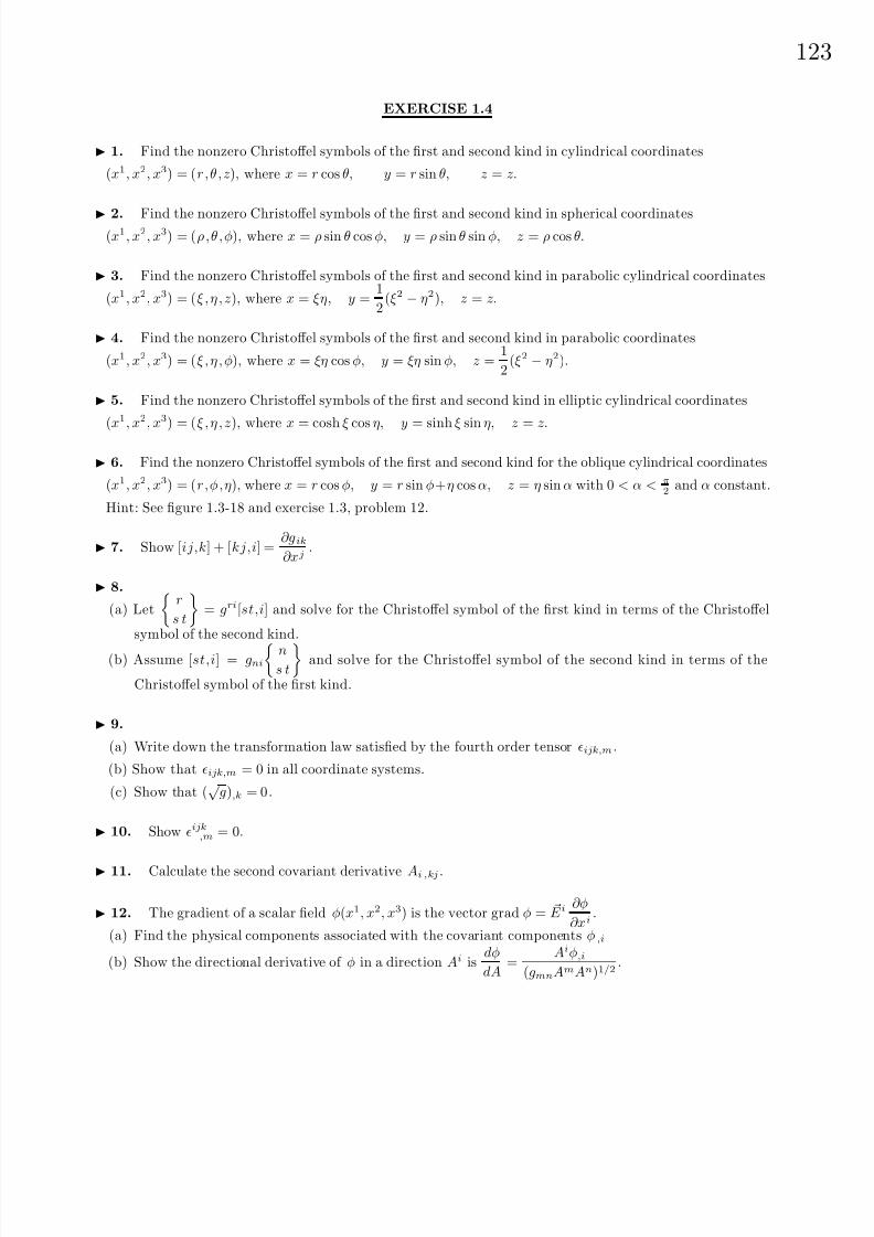
8/6/2019 Introduction to Tensor Calculus Continuum Mechanics - J. Heinbockel
http://slidepdf.com/reader/full/introduction-to-tensor-calculus-continuum-mechanics-j-heinbockel 128/372
12
EXERCISE 1.4
1. Find the nonzero Christoffel symbols of the first and second kind in cylindrical coordinates
(x1, x2, x3) = (r,θ,z), where x = r cos θ, y = r sin θ, z = z.
2. Find the nonzero Christoffel symbols of the first and second kind in spherical coordinates(x1, x2, x3) = (ρ ,θ,φ), where x = ρ sin θ cos φ, y = ρ sin θ sin φ, z = ρ cos θ.
3. Find the nonzero Christoffel symbols of the first and second kind in parabolic cylindrical coordinates
(x1, x2, x3) = (ξ , η , z), where x = ξη, y =1
2(ξ2 − η2), z = z.
4. Find the nonzero Christoffel symbols of the first and second kind in parabolic coordinates
(x1, x2, x3) = (ξ , η , φ), where x = ξη cos φ, y = ξη sin φ, z =1
2(ξ2 − η2).
5. Find the nonzero Christoffel symbols of the first and second kind in elliptic cylindrical coordinates
(x1, x2, x3) = (ξ , η , z), where x = cosh ξ cos η, y = sinh ξ sin η, z = z.
6. Find the nonzero Christoffel symbols of the first and second kind for the oblique cylindrical coordinates
(x1, x2, x3) = (r,φ,η), where x = r cos φ, y = r sin φ+η cos α, z = η sin α with 0 < α < π2 and α constant.
Hint: See figure 1.3-18 and exercise 1.3, problem 12.
7. Show [ij,k] + [kj,i] =∂gik
∂xj.
8.
(a) Let
r
s t
= gri[st,i] and solve for the Christoffel symbol of the first kind in terms of the Christoffel
symbol of the second kind.
(b) Assume [st,i] = gni
n
s t
and solve for the Christoffel symbol of the second kind in terms of the
Christoffel symbol of the first kind.
9.
(a) Write down the transformation law satisfied by the fourth order tensor ijk,m.
(b) Show that ijk,m = 0 in all coordinate systems.
(c) Show that (√
g),k = 0.
10. Show ijk,m = 0.
11. Calculate the second covariant derivative Ai ,kj .
12. The gradient of a scalar field φ(x1, x2, x3) is the vector grad φ = E i∂φ
∂xi.
(a) Find the physical components associated with the covariant components φ ,i
(b) Show the directional derivative of φ in a direction Ai isdφ
dA=
Aiφ,i
(gmnAmAn)1/2.

8/6/2019 Introduction to Tensor Calculus Continuum Mechanics - J. Heinbockel
http://slidepdf.com/reader/full/introduction-to-tensor-calculus-continuum-mechanics-j-heinbockel 129/372
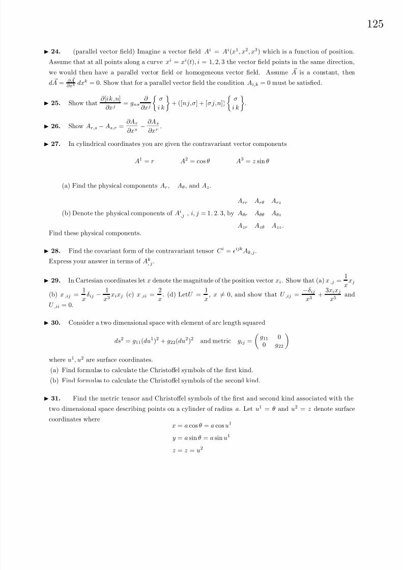
8/6/2019 Introduction to Tensor Calculus Continuum Mechanics - J. Heinbockel
http://slidepdf.com/reader/full/introduction-to-tensor-calculus-continuum-mechanics-j-heinbockel 130/372
12
24. (parallel vector field) Imagine a vector field Ai = Ai(x1, x2, x3) which is a function of position.
Assume that at all points along a curve xi = xi(t), i = 1, 2, 3 the vector field points in the same direction,
we would then have a parallel vector field or homogeneous vector field. Assume A is a constant, then
d A = ∂ A∂xk dxk = 0. Show that for a parallel vector field the condition Ai,k = 0 must be satisfied.
25. Show that ∂ [ik,n]∂xj
= gnσ ∂ ∂xj
σ
i k
+ ([nj,σ] + [σj,n])
σ
i k
.
26. Show Ar,s − As,r =∂Ar
∂xs− ∂As
∂xr.
27. In cylindrical coordinates you are given the contravariant vector components
A1 = r A2 = cos θ A3 = z sin θ
(a) Find the physical components Ar, Aθ, and Az.
(b) Denote the physical components of Ai,j , i, j = 1, 2, 3, by
Arr Arθ Arz
Aθr Aθθ Aθz
Azr Azθ Azz .Find these physical components.
28. Find the covariant form of the contravariant tensor C i = ijk Ak,j.
Express your answer in terms of Ak, j .
29. In Cartesian coordinates let x denote the magnitude of the position vector xi. Show that (a) x ,j =1
xxj
(b) x ,ij =1
x
δij
−1
x3
xixj (c) x ,ii =2
x
. (d) LetU =1
x
, x
= 0, and show that U ,ij =
−δij
x3
+3xixj
x5
and
U ,ii = 0.
30. Consider a two dimensional space with element of arc length squared
ds2 = g11(du1)2 + g22(du2)2 and metric gij =
g11 0
0 g22
where u1, u2 are surface coordinates.
(a) Find formulas to calculate the Christoffel symbols of the first kind.
(b) Find formulas to calculate the Christoffel symbols of the second kind.
31. Find the metric tensor and Christoffel symbols of the first and second kind associated with thetwo dimensional space describing points on a cylinder of radius a. Let u1 = θ and u2 = z denote surface
coordinates wherex = a cos θ = a cos u1
y = a sin θ = a sin u1
z = z = u2

8/6/2019 Introduction to Tensor Calculus Continuum Mechanics - J. Heinbockel
http://slidepdf.com/reader/full/introduction-to-tensor-calculus-continuum-mechanics-j-heinbockel 131/372
126
32. Find the metric tensor and Christoffel symbols of the first and second kind associated with the
two dimensional space describing points on a sphere of radius a. Let u1 = θ and u2 = φ denote surface
coordinates wherex = a sin θ cos φ = a sin u1 cos u2
y = a sin θ sin φ = a sin u1 sin u2
z = a cos θ = a cos u1
33. Find the metric tensor and Christoffel symbols of the first and second kind associated with the
two dimensional space describing points on a torus having the parameters a and b and surface coordinates
u1 = ξ, u2 = η. illustrated in the figure 1.3-19. The points on the surface of the torus are given in terms
of the surface coordinates by the equations
x = (a + b cos ξ)cos η
y = (a + b cos ξ)sin η
z = b sin ξ
34. Prove that eijk ambjckui,m + eijkaibmckuj
,m + eijk aibjcmuk,m = ur
,reijk aibjck. Hint: See Exercise 1.3,
problem 32 and Exercise 1.1, problem 21.
35. Calculate the second covariant derivative Ai,jk .
36. Show that σij,j =
1√g
∂
∂xj
√gσij
+ σmn
i
m n
37. Find the contravariant, covariant and physical components of velocity and acceleration in (a) Cartesian
coordinates and (b) cylindrical coordinates.
38. Find the contravariant, covariant and physical components of velocity and acceleration in spherical
coordinates.
39. In spherical coordinates (ρ ,θ,φ) show that the acceleration components can be represented in terms
of the velocity components as
f ρ = vρ −v2
θ + v2φ
ρ, f θ = vθ +
vρvθ
ρ− v2
φ
ρ tan θ, f φ = vφ +
vρvφ
ρ+
vθvφ
ρ tan θ
Hint: Calculate vρ, vθ, vφ.
40. The divergence of a vector Ai is Ai,i. That is, perform a contraction on the covariant derivative
Ai,j to obtain Ai
,i. Calculate the divergence in (a) Cartesian coordinates (b) cylindrical coordinates and (c)
spherical coordinates.
41. If S is a scalar invariant of weight one and Aijk is a third order relative tensor of weight W , show
that S −W Aijk is an absolute tensor.
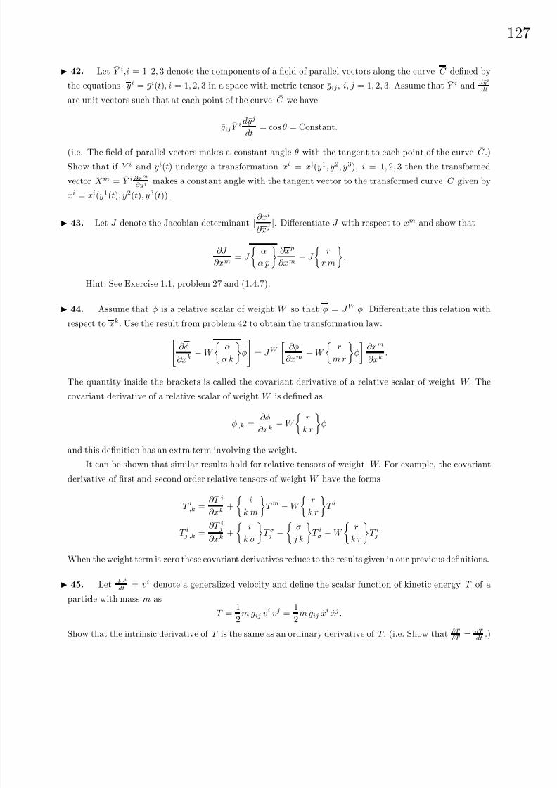
8/6/2019 Introduction to Tensor Calculus Continuum Mechanics - J. Heinbockel
http://slidepdf.com/reader/full/introduction-to-tensor-calculus-continuum-mechanics-j-heinbockel 132/372
12
42. Let Y i,i = 1, 2, 3 denote the components of a field of parallel vectors along the curve C defined by
the equations yi = yi(t), i = 1, 2, 3 in a space with metric tensor gij, i, j = 1, 2, 3. Assume that Y i and dyi
dt
are unit vectors such that at each point of the curve C we have
gij Y idyj
dt= cos θ = Constant.
(i.e. The field of parallel vectors makes a constant angle θ with the tangent to each point of the curve C .)
Show that if Y i and yi(t) undergo a transformation xi = xi(y1, y2, y3), i = 1, 2, 3 then the transformed
vector X m = Y i ∂xm
∂ yj makes a constant angle with the tangent vector to the transformed curve C given by
xi = xi(y1(t), y2(t), y3(t)).
43. Let J denote the Jacobian determinant | ∂xi
∂xj |. Differentiate J with respect to xm and show that
∂J
∂xm= J
α
α p
∂x p
∂xm− J
r
r m
.
Hint: See Exercise 1.1, problem 27 and (1.4.7).
44. Assume that φ is a relative scalar of weight W so that φ = J W φ. Differentiate this relation with
respect to xk. Use the result from problem 42 to obtain the transformation law:∂φ
∂xk− W
α
α k
φ
= J W
∂φ
∂xm− W
r
m r
φ
∂xm
∂xk.
The quantity inside the brackets is called the covariant derivative of a relative scalar of weight W. The
covariant derivative of a relative scalar of weight W is defined as
φ ,k =∂φ
∂xk− W
r
k r
φ
and this definition has an extra term involving the weight.
It can be shown that similar results hold for relative tensors of weight W. For example, the covariant
derivative of first and second order relative tensors of weight W have the forms
T i,k =∂T i
∂xk+
i
k m
T m − W
r
k r
T i
T ij ,k =∂T ij
∂xk+
i
k σ
T σj −
σ
j k
T iσ − W
r
k r
T ij
When the weight term is zero these covariant derivatives reduce to the results given in our previous definitions.
45. Let dxi
dt = vi denote a generalized velocity and define the scalar function of kinetic energy T of a
particle with mass m as
T =1
2m gij vi vj =
1
2m gij xi xj .
Show that the intrinsic derivative of T is the same as an ordinary derivative of T. (i.e. Show that δT δT
= dT dt
.)

8/6/2019 Introduction to Tensor Calculus Continuum Mechanics - J. Heinbockel
http://slidepdf.com/reader/full/introduction-to-tensor-calculus-continuum-mechanics-j-heinbockel 133/372
128
46. Verify the relations∂gij
∂xk= −gmj gni
∂g nm
∂xk
∂g in
∂xk= −gmn gij ∂gjm
∂xk
47. Assume that Bijk is an absolute tensor. Is the quantity T jk = 1√g
∂ ∂xi
√gBijk
a tensor? Justify
your answer. If your answer is “no”, explain your answer and determine if there any conditions you can
impose upon Bijk such that the above quantity will be a tensor?
48. The e-permutation symbol can be used to define various vector products. Let Ai, Bi, C i, Di
i = 1, . . . , N denote vectors, then expand and verify the following products:
(a) In two dimensionsR =eijAiBj a scalar determinant.
Ri =eijAj a vector (rotation).
(b) In three dimensionsS =eijkAiBj C k a scalar determinant.
S i =eijkBj C k a vector cross product.
S ij =eijkC k a skew-symmetric matrix
(c) In four dimensions
T =eijkmAiBjC kDm a scalar determinant.
T i =eijkmBj C kDm 4-dimensional cross product.
T ij =eijkmC kDm skew-symmetric matrix.
T ijk =eikmDm skew-symmetric tensor.
with similar products in higher dimensions.
49. Expand the curl operator for:
(a) Two dimensions B = eij Aj,i
(b) Three dimensions Bi = eijk Ak,j
(c) Four dimensions Bij = eijkmAm,k

8/6/2019 Introduction to Tensor Calculus Continuum Mechanics - J. Heinbockel
http://slidepdf.com/reader/full/introduction-to-tensor-calculus-continuum-mechanics-j-heinbockel 134/372
12
§1.5 DIFFERENTIAL GEOMETRY AND RELATIVITY
In this section we will examine some fundamental properties of curves and surfaces. In particular, at
each point of a space curve we can construct a moving coordinate system consisting of a tangent vector, a
normal vector and a binormal vector which is perpendicular to both the tangent and normal vectors. How
these vectors change as we move along the space curve brings up the subjects of curvature and torsion
associated with a space curve. The curvature is a measure of how the tangent vector to the curve is changing
and the torsion is a measure of the twisting of the curve out of a plane. We will find that straight lines have
zero curvature and plane curves have zero torsion.
In a similar fashion, associated with every smooth surface there are two coordinate surface curves and
a normal surface vector through each point on the surface. The coordinate surface curves have tangent
vectors which together with the normal surface vectors create a set of basis vectors. These vectors can be
used to define such things as a two dimensional surface metric and a second order curvature tensor. The
coordinate curves have tangent vectors which together with the surface normal form a coordinate system at
each point of the surface. How these surface vectors change brings into consideration two different curvatures.
A normal curvature and a tangential curvature (geodesic curvature). How these curvatures are related tothe curvature tensor and to the Riemann Christoffel tensor, introduced in the last section, as well as other
interesting relationships between the various surface vectors and curvatures, is the subject area of differential
geometry.
Also presented in this section is a brief introduction to relativity where again the Riemann Christoffel
tensor will occur. Properties of this important tensor are developed in the exercises of this section.
Space Curves and Curvature
For xi = xi(s),i = 1, 2, 3, a 3-dimensional space curve in a Riemannian space V n with metric tensor gij ,
and arc length parameter s, the vector T i = dxi
ds represents a tangent vector to the curve at a point P on
the curve. The vector T i is a unit vector because
gijT iT j = gijdxi
ds
dxj
ds= 1. (1.5.1)
Differentiate intrinsically, with respect to arc length, the relation (1.5.1) and verify that
gij T iδT j
δs+ gij
δT i
δsT j = 0, (1.5.2)
which implies that
gijT jδT i
δs= 0. (1.5.3)
Hence, the vectorδT i
δs is perpendicular to the tangent vector T i
. Define the unit normal vector N i
to thespace curve to be in the same direction as the vector δT i
δs and write
N i =1
κ
δT i
δs(1.5.4)
where κ is a scale factor, called the curvature, and is selected such that
gijN iN j = 1 which implies gijδT i
δs
δT j
δs= κ2. (1.5.5)

8/6/2019 Introduction to Tensor Calculus Continuum Mechanics - J. Heinbockel
http://slidepdf.com/reader/full/introduction-to-tensor-calculus-continuum-mechanics-j-heinbockel 135/372
130
The reciprocal of curvature is called the radius of curvature. The curvature measures the rate of change of
the tangent vector to the curve as the arc length varies. By differentiating intrinsically, with respect to arc
length s, the relation gijT iN j = 0 we find that
gijT iδN j
δs+ gij
δT i
δsN j = 0. (1.5.6)
Consequently, the curvature κ can be determined from the relation
gijT iδN j
δs= −gij
δT i
δsN j = −gijκN iN j = −κ (1.5.7)
which defines the sign of the curvature. In a similar fashion we differentiate the relation (1.5.5) and find that
gijN iδN j
δs= 0. (1.5.8)
This later equation indicates that the vector δN j
δs is perpendicular to the unit normal N i. The equation
(1.5.3) indicates that T i is also perpendicular to N i and hence any linear combination of these vectors will
also be perpendicular to N i. The unit binormal vector is defined by selecting the linear combination
δN j
δs+ κT j (1.5.9)
and then scaling it into a unit vector by defining
Bj =1
τ
δN j
δs+ κT j
(1.5.10)
where τ is a scalar called the torsion. The sign of τ is selected such that the vectors T i, N i and Bi form a
right handed system with ijkT iN j Bk = 1 and the magnitude of τ is selected such that Bi is a unit vector
satisfying
gijBiBj = 1. (1.5.11)
The triad of vectors T i, N i, Bi at a point on the curve form three planes. The plane containing T i and Bi is
called the rectifying plane. The plane containing N i and Bi is called the normal plane. The plane containing
T i and N i is called the osculating plane. The reciprocal of the torsion is called the radius of torsion. The
torsion measures the rate of change of the osculating plane. The vectors T i, N i and Bi form a right-handed
orthogonal system at a point on the space curve and satisfy the relation
Bi = ijk T j N k. (1.5.12)
By using the equation (1.5.10) it can be shown that Bi is perpendicular to both the vectors T i and N i since
gij BiT j = 0 and gijBiN j = 0.
It is left as an exercise to show that the binormal vector Bi satisfies the relation δBi
δs = −τ N i. The three
relationsδT i
δs= κN i
δN i
δs= τBi − κT i
δBi
δs= −τ N i
(1.5.13)

8/6/2019 Introduction to Tensor Calculus Continuum Mechanics - J. Heinbockel
http://slidepdf.com/reader/full/introduction-to-tensor-calculus-continuum-mechanics-j-heinbockel 136/372

8/6/2019 Introduction to Tensor Calculus Continuum Mechanics - J. Heinbockel
http://slidepdf.com/reader/full/introduction-to-tensor-calculus-continuum-mechanics-j-heinbockel 137/372
132
and is such that the vectors E 1, E 2 and n form a right-handed system of coordinates.
If we transform from one set of curvilinear coordinates (u, v) to another set (u, v), which are determined
by a set of transformation laws
u = u(u, v), v = v(u, v),
the equation of the surface becomes
r = r(u, v) = x(u(u, v), v(u, v)) e1 + y(u(u, v), v(u, v)) e2 + z(u(u, v), v(u, v)) e3and the tangent vectors to the new coordinate curves are
∂r
∂ u=
∂r
∂u
∂u
∂ u+
∂r
∂v
∂v
∂ uand
∂r
∂ v=
∂r
∂u
∂u
∂ v+
∂r
∂v
∂v
∂ v.
Using the indicial notation this result can be represented as
∂y i
∂ uα=
∂y i
∂uβ
∂uβ
∂ uα.
This is the transformation law connecting the two systems of basis vectors on the surface.
A curve on the surface is defined by a relation f (u, v) = 0 between the curvilinear coordinates. Another
way to represent a curve on the surface is to represent it in a parametric form where u = u(t) and v = v(t),
where t is a parameter. The vectordr
dt=
∂r
∂u
du
dt+
∂r
∂v
dv
dt
is tangent to the curve on the surface.
An element of arc length with respect to the surface coordinates is represented by
ds2 = dr · dr =∂r
∂uα· ∂r
∂uβduα duβ = aαβduαduβ (1.5.19)
where aαβ = ∂r∂uα
·∂r
∂uβ with α, β = 1, 2 defines a surface metric. This element of arc length on the surface is
often written as the quadratic form
A = ds2 = E (du)2 + 2Fdudv + G(dv)2 =1
E (E du + F dv)2 +
EG − F 2
E dv2 (1.5.20)
and called the first fundamental form of the surface. Observe that for ds2 to be positive definite the quantities
E and EG − F 2 must be positive.
The surface metric associated with the two dimensional surface is defined by
aαβ = E α · E β =∂r
∂uα· ∂r
∂uβ=
∂y i
∂uα
∂y i
∂uβ, α, β = 1, 2 (1.5.21)
with conjugate metric tensor aαβ defined such that aαβaβγ = δαγ . Here the surface is embedded in a three
dimensional space with metric gij and aαβ is the two dimensional surface metric. In the equation (1.5.20)
the quantities E, F , G are functions of the surface coordinates u, v and are determined from the relations
E =a11 =∂r
∂u· ∂r
∂u=
∂y i
∂u1
∂y i
∂u1
F =a12 =∂r
∂u· ∂r
∂v=
∂y i
∂u1
∂y i
∂u2
G =a22 =∂r
∂v· ∂r
∂v=
∂y i
∂u2
∂y i
∂u2
(1.5.22)

8/6/2019 Introduction to Tensor Calculus Continuum Mechanics - J. Heinbockel
http://slidepdf.com/reader/full/introduction-to-tensor-calculus-continuum-mechanics-j-heinbockel 138/372
13
Here and throughout the remainder of this section, we adopt the convention that Greek letters have the
range 1,2, while Latin letters have the range 1,2,3.
Construct at a general point P on the surface the unit normal vector n at this point. Also construct a
plane which contains this unit surface normal vector
n. Observe that there are an infinite number of planes
which contain this unit surface normal. For now, select one of these planes, then later on we will consider
all such planes. Let r = r(s) denote the position vector defining a curve C which is the intersection of the
selected plane with the surface, where s is the arc length along the curve, which is measured from some fixed
point on the curve. Let us find the curvature of this curve of intersection. The vector T = drds , evaluated
at the point P, is a unit tangent vector to the curve C and lies in the tangent plane to the surface at the
point P. Here we are using ordinary differentiation rather than intrinsic differentiation because we are in
a Cartesian system of coordinates. Differentiating the relation T · T = 1, with respect to arc length s we
find that T · d T ds = 0 which implies that the vector d T
ds is perpendicular to the tangent vector T . Since the
coordinate system is Cartesian we can treat the curve of intersection C as a space curve, then the vector
K = d
T
ds , evaluated at point P, is defined as the curvature vector with curvature | K | = κ and radius of
curvature R = 1/κ. A unit normal N to the space curve is taken in the same direction asd T
ds so that the
curvature will always be positive. We can then write K = κ N =d T
ds. Consider the geometry of figure 1.5-1
and define on the surface a unit vector u = n× T which is perpendicular to both the surface tangent vector T and the surface normal vector n, such that the vectors T i,ui and ni forms a right-handed system.
Figure 1.5-1 Surface curve with tangent plane and a normal plane.

8/6/2019 Introduction to Tensor Calculus Continuum Mechanics - J. Heinbockel
http://slidepdf.com/reader/full/introduction-to-tensor-calculus-continuum-mechanics-j-heinbockel 139/372
134
The direction of u in relation to T is in the same sense as the surface tangents E 1 and E 2. Note that
the vector d T ds is perpendicular to the tangent vector T and lies in the plane which contains the vectors n
and u. We can therefore write the curvature vector K in the component form
K =d
T
ds
= κ(n) n + κ(g) u = K n + K g (1.5.23)
where κ(n) is called the normal curvature and κ(g) is called the geodesic curvature. The subscripts are not
indices. These curvatures can be calculated as follows. From the orthogonality condition n · T = 0 we obtain
by differentiation with respect to arc length s the result n · d T
ds+ T · d n
ds= 0. Consequently, the normal
curvature is determined from the dot product relation
n · K = κ(n) = − T · d nds
= −dr
ds· d n
ds. (1.5.24)
By taking the dot product of
u with equation (1.5.23) we find that the geodesic curvature is determined
from the triple scalar product relation
κ(g) = u · d T
ds= ( n × T ) · d T
ds. (1.5.25)
Normal Curvature
The equation (1.5.24) can be expressed in terms of a quadratic form by writing
κ(n) ds2 = −dr · d n. (1.5.26)
The unit normal to the surface
n and position vector r are functions of the surface coordinates u, v with
dr =
∂r
∂u du +
∂r
∂v dv and d n =
∂ n∂u du +
∂ n∂v dv. (1.5.27)
We define the quadratic form
B = −dr · d n = −
∂r
∂udu +
∂r
∂vdv
·
∂ n∂u
du +∂ n∂v
dv
B = e(du)2 + 2fdudv + g(dv)2 = bαβ duαduβ
(1.5.28)
where
e = − ∂r
∂u· ∂ n
∂u, 2f = −
∂r
∂u· ∂ n
∂v+
∂ n∂u
· ∂r
∂v
, g = −∂r
∂v· ∂ n
∂v(1.5.29)
and bαβ α, β = 1, 2 is called the curvature tensor and aαγbαβ = bγβ is an associated curvature tensor.
The quadratic form of equation (1.5.28) is called the second fundamental form of the surface. Alternative
methods for calculating the coefficients of this quadratic form result from the following considerations. The
unit surface normal is perpendicular to the tangent vectors to the coordinate curves at the point P and
therefore we have the orthogonality relationships
∂r
∂u· n = 0 and
∂r
∂v· n = 0. (1.5.30)

8/6/2019 Introduction to Tensor Calculus Continuum Mechanics - J. Heinbockel
http://slidepdf.com/reader/full/introduction-to-tensor-calculus-continuum-mechanics-j-heinbockel 140/372
13
Observe that by differentiating the relations in equation (1.5.30), with respect to both u and v, one can
derive the results
e =∂ 2r
∂u2· n = −∂r
∂u· ∂ n
∂u= b11
f =∂ 2r
∂u∂v·
n = − ∂r
∂u· ∂
n
∂v= −∂
n
∂u· ∂r
∂v= b21 = b12
g = ∂ 2r∂v2
· n = −∂r∂v
· ∂ n∂v
= b22
(1.5.31)
and consequently the curvature tensor can be expressed as
bαβ = − ∂r
∂uα· ∂ n
∂uβ. (1.5.32)
The quadratic forms from equations (1.5.20) and (1.5.28) enable us to represent the normal curvature
in the form of a ratio of quadratic forms. We find from equation (1.5.26) that the normal curvature in the
direction dudv is
κ(n) =B
A=
e(du)2 + 2f dudv + g(dv)2
E (du)2 + 2F dudv + G(dv)2. (1.5.33)
If we write the unit tangent vector to the curve in the form T = drds = ∂r
∂uαduα
ds and express the derivative
of the unit surface normal with respect to arc length as d nds = ∂ n
∂uβduβ
ds , then the normal curvature can be
expressed in the form
κ(n) = − T · d nds
= −
∂r
∂uα· ∂ n
∂uβ
duα
ds
duβ
ds
=bαβduαduβ
ds2=
bαβduαduβ
aαβduαduβ.
(1.5.34)
Observe that the curvature tensor is a second order symmetric tensor.
In the previous discussions, the plane containing the unit normal vector was arbitrary. Let us now
consider all such planes that pass through this unit surface normal. As we vary the plane containing the unit
surface normal n at P we get different curves of intersection with the surface. Each curve has a curvature
associated with it. By examining all such planes we can find the maximum and minimum normal curvatures
associated with the surface. We write equation (1.5.33) in the form
κ(n) =e + 2f λ + gλ2
E + 2F λ + Gλ2(1.5.35)
where λ = dvdu
. From the theory of proportions we can also write this equation in the form
κ(n) =(e + f λ) + λ(f + gλ)
(E + F λ) + λ(F + Gλ)=
f + gλ
F + Gλ=
e + f λ
E + F λ. (1.5.36)
Consequently, the curvature κ will satisfy the differential equations
(e − κE )du + (f − κF )dv = 0 and (f − κF )du + (g − κG)dv = 0. (1.5.37)
The maximum and minimum curvatures occur in those directions λ wheredκ(n)
dλ = 0. Calculating the deriva-
tive of κ(n) with respect to λ and setting the derivative to zero we obtain a quadratic equation in λ
(F g − Gf )λ2 + (Eg − Ge)λ + (Ef − F e) = 0, (F g − Gf ) = 0.
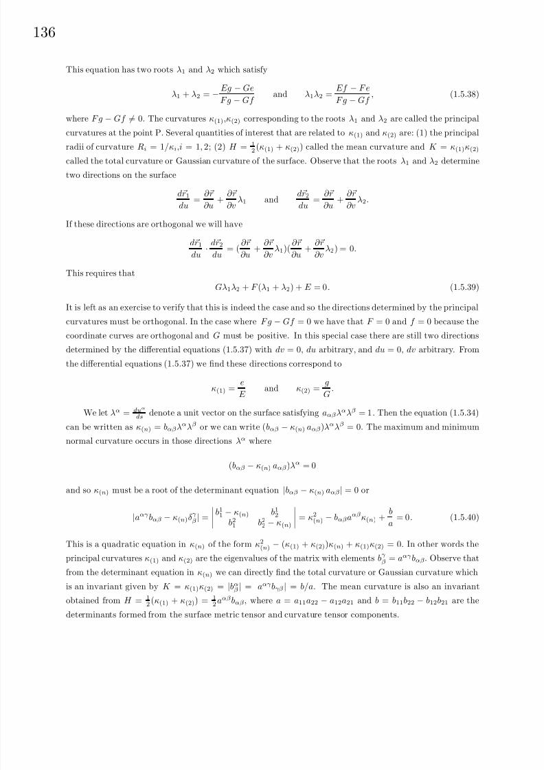
8/6/2019 Introduction to Tensor Calculus Continuum Mechanics - J. Heinbockel
http://slidepdf.com/reader/full/introduction-to-tensor-calculus-continuum-mechanics-j-heinbockel 141/372

8/6/2019 Introduction to Tensor Calculus Continuum Mechanics - J. Heinbockel
http://slidepdf.com/reader/full/introduction-to-tensor-calculus-continuum-mechanics-j-heinbockel 142/372
13
The equations of Gauss, Weingarten and Codazzi
At each point on a space curve we can construct a unit tangent T , a unit normal N and unit binormal
B. The derivatives of these vectors, with respect to arc length, can also be represented as linear combinations
of the base vectors T , N , B. See for example the Frenet-Serret formulas from equations (1.5.13). In a similar
fashion the surface vectors ru, rv, n form a basis and the derivatives of these basis vectors with respect to
the surface coordinates u, v can also be expressed as linear combinations of the basis vectors ru, rv, n. For
example, the derivatives ruu, ruv, rvv can be expressed as linear combinations of ru, rv, n. We can write
ruu = c1ru + c2rv + c3 nruv = c4ru + c5rv + c6 nrvv = c7ru + c8rv + c9 n
(1.5.41)
where c1, . . . , c9 are constants to be determined. It is an easy exercise (see exercise 1.5, problem 8) to show
that these equations can be written in the indicial notation as
∂ 2r
∂uα∂uβ
= γ
α β ∂r
∂uγ
+ bαβ n. (1.5.42)
These equations are known as the Gauss equations.
In a similar fashion the derivatives of the normal vector can be represented as linear combinations of
the surface basis vectors. If we write
∂ n∂u
= c1ru + c2rv
∂ n∂v
= c3ru + c4rv
or
∂r
∂u= c∗1
∂ n∂u
+ c∗2∂ n∂v
∂r
∂v= c∗3
∂ n∂u
+ c∗4∂ n∂v
(1.5.43)
where c1, . . . , c4 and c∗1, . . . , c∗4 are constants. These equations are known as the Weingarten equations. It
is easily demonstrated (see exercise 1.5, problem 9) that the Weingarten equations can be written in the
indicial form∂ n
∂uα= −bβ
α
∂r
∂uβ(1.5.44)
where bβα = aβγ bγα is the mixed second order form of the curvature tensor.
The equations of Gauss produce a system of partial differential equations defining the surface coordinates
xi as a function of the curvilinear coordinates u and v. The equations are not independent as certain
compatibility conditions must be satisfied. In particular, it is required that the mixed partial derivatives
must satisfy∂ 3r
∂uα∂uβ∂uδ=
∂ 3r
∂uα∂uδ∂uβ.
We calculate
∂ 3r
∂uα∂uβ∂uδ=
γ
α β
∂ 2r
∂uγ∂uδ+
∂ γα β
∂uδ
∂r
∂uγ+ bαβ
∂ n∂uδ
+∂bαβ
∂uδn
and use the equations of Gauss and Weingarten to express this derivative in the form
∂ 3r
∂uα∂uβ∂uδ=
∂
ω
α β
∂uδ
+
γ
α β
ω
γ δ
− bαβbω
δ
∂r
∂uω+
γ
α β
bγδ +
∂bαβ
∂uδ
n.
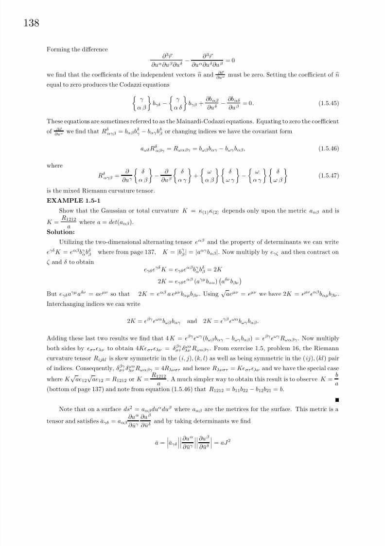
8/6/2019 Introduction to Tensor Calculus Continuum Mechanics - J. Heinbockel
http://slidepdf.com/reader/full/introduction-to-tensor-calculus-continuum-mechanics-j-heinbockel 143/372
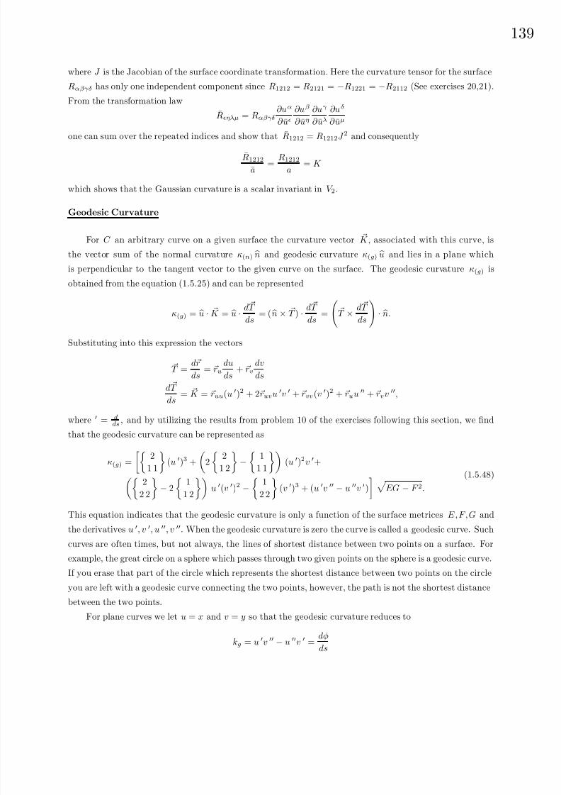
8/6/2019 Introduction to Tensor Calculus Continuum Mechanics - J. Heinbockel
http://slidepdf.com/reader/full/introduction-to-tensor-calculus-continuum-mechanics-j-heinbockel 144/372

8/6/2019 Introduction to Tensor Calculus Continuum Mechanics - J. Heinbockel
http://slidepdf.com/reader/full/introduction-to-tensor-calculus-continuum-mechanics-j-heinbockel 145/372
140
where φ is the angle between the tangent T to the curve and the unit vector e1.
Geodesics are curves on the surface where the geodesic curvature is zero. Since kg = 0 along a geodesic
surface curve, then at every point on this surface curve the normal N to the curve will be in the same
direction as the normal
n to the surface. In this case, we have ru ·
n = 0 and rv ·
n = 0 which reduces to
d T ds
· ru = 0 and d T ds
· rv = 0, (1.5.49)
since the vectors n and d T ds have the same direction. In particular, we may write
T =dr
ds=
∂r
∂u
du
ds+
∂r
∂v
dv
ds= ru u + rv v
d T
ds= ruu (u )2 + 2ruv u v + rvv (v )2 + ru u + rv v
Consequently, the equations (1.5.49) become
d T
ds · ru = (ruu · ru) (u
)2 + 2(ruv · ru) u
v
+ (rvv · ru) (v
)2 + Eu
+ F v
= 0
d T
ds· rv = (ruu · rv) (u )2 + 2(ruv · rv) u v + (rvv · rv) (v )2 + F u + Gv = 0.
. (1.5.50)
Utilizing the results from exercise 1.5,(See problems 4,5 and 6), we can eliminate v from the equations
(1.5.50) to obtain
d2u
ds2+
1
1 1
du
ds
2
+ 2
1
1 2
du
ds
dv
ds+
1
2 2
dv
ds
2
= 0
and eliminating u from the equations (1.5.50) produces the equation
d2v
ds2+ 2
1 1du
ds2
+ 2 2
1 2 du
ds
dv
ds+ 2
2 2dv
ds2
= 0.
In tensor form, these last two equations are written
d2uα
ds2+
α
β γ
a
duβ
ds
duγ
ds= 0, α, β, γ = 1, 2 (1.5.51)
where u = u1 and v = u2. The equations (1.5.51) are the differential equations defining a geodesic curve on
a surface. We will find that these same type of equations arise in considering the shortest distance between
two points in a generalized coordinate system. See for example problem 18 in exercise 2.2.

8/6/2019 Introduction to Tensor Calculus Continuum Mechanics - J. Heinbockel
http://slidepdf.com/reader/full/introduction-to-tensor-calculus-continuum-mechanics-j-heinbockel 146/372
14
Tensor Derivatives
Let uα = uα(t) denote the parametric equations of a curve on the surface defined by the parametric
equations xi = xi(u1, u2). We can then represent the surface curve in the spatial geometry since the surface
curve can be represented in the spatial coordinates through the representation xi = xi(u1(t), u2(t)) = xi(t).
Recall that for xi = xi(t) a given curve C , the intrinsic derivative of a vector field Ai along C is defined as
the inner product of the covariant derivative of the vector field with the tangent vector to the curve. This
intrinsic derivative is written
δAi
δt= Ai
,j
dxj
dt=
∂Ai
∂xj+
i
j k
g
Ak
dxj
dt
orδAi
δt=
dAi
dt+
i
j k
g
Ak dxj
dt
where the subscript g indicates that the Christoffel symbol is formed from the spatial metric gij. If Aα is a
surface vector defined along the curve C, the intrinsic derivative is represented
δAα
δt= Aα
,β
duβ
dt=∂Aα
∂uβ+ α
β γ
a
Aγ duβ
dt
orδAα
δt=
dAα
dt+
α
β γ
a
Aγ duβ
dt
where the subscript a denotes that the Christoffel is formed from the surface metric aαβ.
Similarly, the formulas for the intrinsic derivative of a covariant spatial vector Ai or covariant surface
vector Aα are given byδAi
δt=
dAi
dt−
k
i j
g
Akdxj
dt
andδAα
δt=
dAα
dt−
γ
α β
a
Aαduβ
dt.
Consider a mixed tensor T iα which is contravariant with respect to a transformation of space coordinates
xi and covariant with respect to a transformation of surface coordinates uα. For T iα defined over the surface
curve C, which can also be viewed as a space curve C, define the scalar invariant Ψ = Ψ( t) = T iαAiBα where
Ai is a parallel vector field along the curve C when it is viewed as a space curve and Bα is also a parallel
vector field along the curve C when it is viewed as a surface curve. Recall that these parallel vector fields
must satisfy the differential equations
δAiδt
= dAidt
− ki j
g
Ak dxj
dt= 0 and δB
α
δt= dB
α
dt+ α
β γ
a
Bγ duβ
dt= 0. (1.5.52)
The scalar invariant Ψ is a function of the parameter t of the space curve since both the tensor and the
parallel vector fields are to be evaluated along the curve C. By differentiating the function Ψ with respect
to the parameter t there results
dΨ
dt=
dT iαdt
AiBα + T iαdAi
dtBα + T iαAi
dBα
dt. (1.5.53)
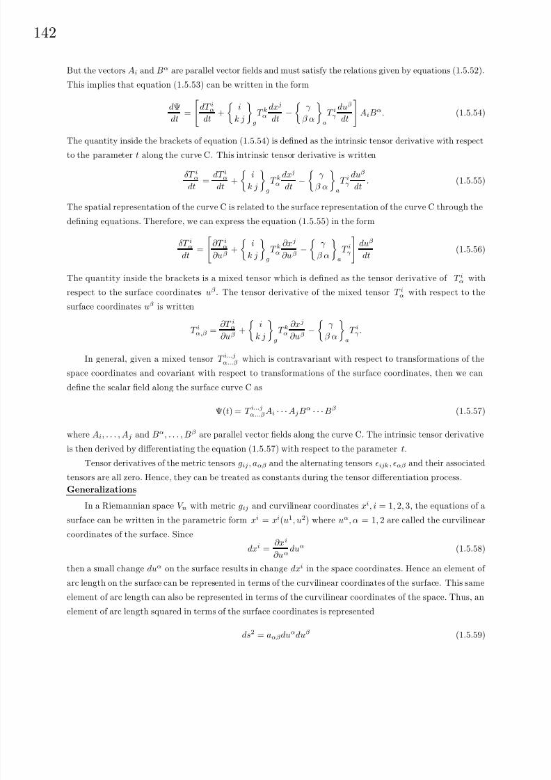
8/6/2019 Introduction to Tensor Calculus Continuum Mechanics - J. Heinbockel
http://slidepdf.com/reader/full/introduction-to-tensor-calculus-continuum-mechanics-j-heinbockel 147/372

8/6/2019 Introduction to Tensor Calculus Continuum Mechanics - J. Heinbockel
http://slidepdf.com/reader/full/introduction-to-tensor-calculus-continuum-mechanics-j-heinbockel 148/372
14
where aαβ is the metric of the surface. This same element when viewed as a spatial element is represented
ds2 = gij dxidxj . (1.5.60)
By equating the equations (1.5.59) and (1.5.60) we find that
gijdxidxj = gij∂xi
∂uα∂xj
∂uβduαduβ = aαβduαduβ . (1.5.61)
The equation (1.5.61) shows that the surface metric is related to the spatial metric and can be calculated
from the relation aαβ = gij∂xi
∂uα
∂xj
∂uβ. This equation reduces to the equation (1.5.21) in the special case of
Cartesian coordinates. In the surface coordinates we define the quadratic form A = aαβduαduβ as the first
fundamental form of the surface. The tangent vector to the coordinate curves defining the surface are given
by ∂xi
∂uα and can be viewed as either a covariant surface vector or a contravariant spatial vector. We define
this vector as
xiα =
∂xi
∂uα, i = 1, 2, 3, α = 1, 2. (1.5.62)
Any vector which is a linear combination of the tangent vectors to the coordinate curves is called a surface
vector. A surface vector Aα can also be viewed as a spatial vector Ai. The relation between the spatial
representation and surface representation is Ai = Aαxiα. The surface representation Aα, α = 1, 2 and the
spatial representation Ai, i = 1, 2, 3 define the same direction and magnitude since
gijAiAj = gij AαxiαAβ xj
β = gij xiαxj
β AαAβ = aαβAαAβ .
Consider any two surface vectors Aα and Bα and their spatial representations Ai and Bi where
Ai = Aαxiα and Bi = Bαxi
α. (1.5.63)
These vectors are tangent to the surface and so a unit normal vector to the surface can be defined from the
cross product relation
niAB sin θ = ijk Aj Bk (1.5.64)
where A, B are the magnitudes of Ai, Bi and θ is the angle between the vectors when their origins are made
to coincide. Substituting equations (1.5.63) into the equation (1.5.64) we find
niAB sin θ = ijk AαxjαBβ xk
β . (1.5.65)
In terms of the surface metric we have AB sin θ = αβAαBβ so that equation (1.5.65) can be written in the
form
(niαβ − ijkxjαxk
β )AαBβ = 0 (1.5.66)
which for arbitrary surface vectors implies
niαβ = ijk xjαxk
β or ni =1
2αβijk xj
αxkβ . (1.5.67)
The equation (1.5.67) defines a unit normal vector to the surface in terms of the tangent vectors to the
coordinate curves. This unit normal vector is related to the covariant derivative of the surface tangents as
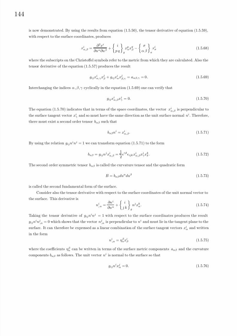
8/6/2019 Introduction to Tensor Calculus Continuum Mechanics - J. Heinbockel
http://slidepdf.com/reader/full/introduction-to-tensor-calculus-continuum-mechanics-j-heinbockel 149/372
144
is now demonstrated. By using the results from equation (1.5.50), the tensor derivative of equation (1.5.59),
with respect to the surface coordinates, produces
xiα,β =
∂ 2xi
∂uα∂uβ+
i
p q
g
x pαxq
β −
σ
α β
a
xiσ (1.5.68)
where the subscripts on the Christoffel symbols refer to the metric from which they are calculated. Also the
tensor derivative of the equation (1.5.57) produces the result
gijxiα,γxj
β + gijxiαxj
β,γ = aαβ,γ = 0. (1.5.69)
Interchanging the indices α, β, γ cyclically in the equation (1.5.69) one can verify that
gijxiα,βxj
γ = 0. (1.5.70)
The equation (1.5.70) indicates that in terms of the space coordinates, the vector xiα,β is perpendicular to
the surface tangent vector xi
γand so must have the same direction as the unit surface normal ni. Therefore,
there must exist a second order tensor bαβ such that
bαβni = xiα,β. (1.5.71)
By using the relation gij ninj = 1 we can transform equation (1.5.71) to the form
bαβ = gijnj xiα,β =
1
2γδ ijk xi
α,βxjγ xk
δ . (1.5.72)
The second order symmetric tensor bαβ is called the curvature tensor and the quadratic form
B = bαβduα
duβ
(1.5.73)
is called the second fundamental form of the surface.
Consider also the tensor derivative with respect to the surface coordinates of the unit normal vector to
the surface. This derivative is
ni, α =
∂ni
∂uα+
i
j k
g
nj xkα. (1.5.74)
Taking the tensor derivative of gijninj = 1 with respect to the surface coordinates produces the result
gij ninj,α = 0 which shows that the vector nj
,α is perpendicular to ni and must lie in the tangent plane to the
surface. It can therefore be expressed as a linear combination of the surface tangent vectors xiα and written
in the formni
,α = ηβαxi
β (1.5.75)
where the coefficients ηβα can be written in terms of the surface metric components aαβ and the curvature
components bαβ as follows. The unit vector ni is normal to the surface so that
gijnixjα = 0. (1.5.76)

8/6/2019 Introduction to Tensor Calculus Continuum Mechanics - J. Heinbockel
http://slidepdf.com/reader/full/introduction-to-tensor-calculus-continuum-mechanics-j-heinbockel 150/372
14
The tensor derivative of this equation with respect to the surface coordinates gives
gijniβxj
α + gij nixjα,β = 0. (1.5.77)
Substitute into equation (1.5.77) the relations from equations (1.5.57), (1.5.71) and (1.5.75) and show that
bαβ = −aαγηγβ . (1.5.78)
Solving the equation (1.5.78) for the coefficients ηγβ we find
ηγβ = −aαγbαβ. (1.5.79)
Now substituting equation (1.5.79) into the equation (1.5.75) produces the Weingarten formula
ni,α = −aγβ bγαxi
β . (1.5.80)
This is a relation for the derivative of the unit normal in terms of the surface metric, curvature tensor andsurface tangents.
A third fundamental form of the surface is given by the quadratic form
C = cαβduαduβ (1.5.81)
where cαβ is defined as the symmetric surface tensor
cαβ = gijni,αnj
,β . (1.5.82)
By using the Weingarten formula in the equation (1.5.81) one can verify that
cαβ = aγδ bαγbβδ . (1.5.83)
Geodesic Coordinates
In a Cartesian coordinate system the metric tensor gij is a constant and consequently the Christoffel
symbols are zero at all points of the space. This is because the Christoffel symbols are dependent upon
the derivatives of the metric tensor which is constant. If the space V N is not Cartesian then the Christoffel
symbols do not vanish at all points of the space. However, it is possible to find a coordinate system where
the Christoffel symbols will all vanish at a given point P of the space. Such coordinates are called geodesic
coordinates of the point P.Consider a two dimensional surface with surface coordinates uα and surface metric aαβ. If we transform
to some other two dimensional coordinate system, say uα with metric aαβ, where the two coordinates are
related by transformation equations of the form
uα = uα(u 1, u 2), α = 1, 2, (1.5.84)

8/6/2019 Introduction to Tensor Calculus Continuum Mechanics - J. Heinbockel
http://slidepdf.com/reader/full/introduction-to-tensor-calculus-continuum-mechanics-j-heinbockel 151/372
146
then from the transformation equation (1.4.7) we can write, after changing symbols,δ
β γ
a
∂uα
∂ u δ=
α
δ
a
∂uδ
∂ u β
∂u
∂ u γ+
∂ 2uα
∂ u β ∂ u γ. (1.5.85)
This is a relationship between the Christoffel symbols in the two coordinate systems. If δ
β γa
vanishes at
a point P , then for that particular point the equation (1.5.85) reduces to
∂ 2uα
∂ u β∂ u γ= −
α
δ
a
∂uδ
∂ u β
∂u
∂ u γ(1.5.86)
where all terms are evaluated at the point P. Conversely, if the equation (1.5.86) is satisfied at the point P,
then the Christoffel symbol
δ
β γ
a
must be zero at this point. Consider the special coordinate transforma-
tion
uα = uα0 + u α − 1
2
α
β γ
a
u β u α (1.5.87)
where uα0 are the surface coordinates of the point P. The point P in the new coordinates is given by
u α = 0. We now differentiate the relation (1.5.87) to see if it satisfies the equation (1.5.86). We calculate
the derivatives∂uα
∂ u τ = δα
τ −1
2
α
β τ
a
uβ − 1
2
α
τ γ
a
uγ
uα=0(1.5.88)
and∂ 2uα
∂ u τ ∂ u σ= −
α
τ σ
a
uα=0
(1.5.89)
where these derivative are evaluated at u α = 0. We find the derivative equations (1.5.88) and (1.5.89) do
satisfy the equation (1.5.86) locally at the point P. Hence, the Christoffel symbols will all be zero at this
particular point. The new coordinates can then be called geodesic coordinates.
Riemann Christoffel Tensor
Consider the Riemann Christoffel tensor defined by the equation (1.4.33). Various properties of this
tensor are derived in the exercises at the end of this section. We will be particularly interested in the
Riemann Christoffel tensor in a two dimensional space with metric aαβ and coordinates uα. We find the
Riemann Christoffel tensor has the form
Rδ. αβγ =
∂
∂uβ
δ
α γ
− ∂
∂uγ
δ
α β
+
τ
α γ
δ
β τ
−
τ
α β
δ
γ τ
(1.5.90)
where the Christoffel symbols are evaluated with respect to the surface metric. The above tensor has the
associated tensor
Rσαβγ = aσδ Rδ. αβγ (1.5.91)
which is skew-symmetric in the indices (σ, α) and (β, γ ) such that
Rσαβγ = −Rασβγ and Rσαβγ = −Rσαγβ . (1.5.92)
The two dimensional alternating tensor is used to define the constant
K =1
4αβγδ Rαβγδ (1.5.93)
8/6/2019 Introduction to Tensor Calculus Continuum Mechanics - J. Heinbockel
http://slidepdf.com/reader/full/introduction-to-tensor-calculus-continuum-mechanics-j-heinbockel 152/372
14
(see example 1.5-1) which is an invariant of the surface and called the Gaussian curvature or total curvature.
In the exercises following this section it is shown that the Riemann Christoffel tensor of the surface can be
expressed in terms of the total curvature and the alternating tensors as
Rαβγδ = Kαβγδ . (1.5.94)
Consider the second tensor derivative of xrα which is given by
xrα,βγ =
∂xrα,β
∂uγ+
r
m n
g
xrα,βxn
γ −
δ
α γ
a
xrδ,β −
δ
β γ
a
xrα,γ (1.5.95)
which can be shown to satisfy the relation
xrα,βγ − xr
α,γβ = Rδ.αβγ xr
δ. (1.5.96)
Using the relation (1.5.96) we can now derive some interesting properties relating to the tensors aαβ, bαβ,
cαβ, Rαβγδ, the mean curvature H and the total curvature K.
Consider the tensor derivative of the equation (1.5.71) which can be written
xiα,βγ = bαβ,γ ni + bαβni
,γ (1.5.97)
where
bαβ,γ =∂bαβ
∂uα−
σ
α γ
a
bσβ −
σ
β γ
a
bασ. (1.5.98)
By using the Weingarten formula, given in equation (1.5.80), the equation (1.5.97) can be expressed in the
form
xiα,βγ = bαβ,γ ni − bαβaτ σbτ γxi
σ (1.5.99)
and by using the equations (1.5.98) and (1.5.99) it can be established that
xrα,βγ − xr
α,γβ = (bαβ,γ − bαγ,β)nr − aτ δ(bαβbτ γ − bαγbτ β)xrδ. (1.5.100)
Now by equating the results from the equations (1.5.96) and (1.5.100) we arrive at the relation
Rδ.αβγ xr
δ = (bαβ,γ − bαγ,β)nr − aτ δ(bαβbτ γ − bαγbτ β)xrδ. (1.5.101)
Multiplying the equation (1.5.101) by nr and using the results from the equation (1.5.76) there results the
Codazzi equations
bαβ,γ −
bαγ,β
= 0. (1.5.102)
Multiplying the equation (1.5.101) by grmxmσ and simplifying one can derive the Gauss equations of the
surface
Rσαβγ = bαγbσβ − bαβbσγ . (1.5.103)
By using the Gauss equations (1.5.103) the equation (1.5.94) can be written as
Kσαβγ = bαγbσβ − bαβbσγ . (1.5.104)

8/6/2019 Introduction to Tensor Calculus Continuum Mechanics - J. Heinbockel
http://slidepdf.com/reader/full/introduction-to-tensor-calculus-continuum-mechanics-j-heinbockel 153/372
148
Another form of equation (1.5.104) is obtained by using the equation (1.5.83) together with the relation
aαβ = −aσγ σαβγ . It is left as an exercise to verify the resulting form
−Kaαβ = cαβ − aσγ bσγ bαβ. (1.5.106)
Define the quantityH =
1
2aσγ bσγ (1.5.107)
as the mean curvature of the surface, then the equation (1.5.106) can be written in the form
cαβ − 2H bαβ + K aαβ = 0. (1.5.108)
By multiplying the equation (1.5.108) by duαduβ and summing, we find
C − 2H B + K A = 0 (1.5.109)
is a relation connecting the first, second and third fundamental forms.
EXAMPLE 1.5-2
In a two dimensional space the Riemann Christoffel tensor has only one nonzero independent component
R1212. ( See Exercise 1.5, problem number 21.) Consequently, the equation (1.5.104) can be written in the
form K √
ae12√
ae12 = b22b11 − b21b12 and solving for the Gaussian curvature K we find
K =b22b11 − b12b21
a11a22 − a12a21=
b
a=
R1212
a. (1.5.110)
Surface Curvature
For a surface curve uα = uα(s),α = 1, 2 lying upon a surface xi = xi(u1, u2),i = 1, 2, 3, we have a two
dimensional space embedded in a three dimensional space. Thus, if tα =duα
dsis a unit tangent vector to
the surface curve then aαβduα
ds
duβ
ds= aαβtαtβ = 1. This same vector can be represented as the unit tangent
vector to the space curve xi = xi(u1(s), u2(s)) with T i =dxi
ds. That is we will have gij
dxi
ds
dxj
ds= gijT iT j = 1.
The surface vector tα and the space vector T i are related by
T i =∂xi
∂uα
duα
ds= xi
αtα. (1.5.111)
The surface vector tα is a unit vector so that aαβtαtβ = 1. If we differentiate this equation intrinsically with
respect to the parameter s, we find that aαβtα δtβ
δs = 0. This shows that the surface vector δtα
δs is perpendicular
to the surface vector tα. Let uα denote a unit normal vector in the surface plane which is orthogonal to the
tangent vector tα. The direction of uα is selected such that αβtαuβ = 1. Therefore, there exists a scalar κ(g)
such thatδtα
δs= κ(g)uα (1.5.112)
8/6/2019 Introduction to Tensor Calculus Continuum Mechanics - J. Heinbockel
http://slidepdf.com/reader/full/introduction-to-tensor-calculus-continuum-mechanics-j-heinbockel 154/372
14
where κ(g) is called the geodesic curvature of the curve. In a similar manner it can be shown that δuα
δs
is a surface vector orthogonal to tα. Let δuα
δs = αtα where α is a scalar constant to be determined. By
differentiating the relation aαβtαuβ = 0 intrinsically and simplifying we find that α = −κ(g) and therefore
δuα
δs
=
−κ(g)tα. (1.5.113)
The equations (1.5.112) and (1.5.113) are sometimes referred to as the Frenet-Serret formula for a curve
relative to a surface.
Taking the intrinsic derivative of equation (1.5.111), with respect to the parameter s, we find that
δT i
δs= xi
α
δtα
δs+ xi
α,β
duβ
dstα. (1.5.114)
Treating the curve as a space curve we use the Frenet formulas (1.5.13). If we treat the curve as a surface
curve, then we use the Frenet formulas (1.5.112) and (1.5.113). In this way the equation (1.5.114) can be
written in the form
κN i = xiακ(g)uα + xiα,βtβtα. (1.5.115)
By using the results from equation (1.5.71) in equation (1.5.115) we obtain
κN i = κ(g)ui + bαβnitαtβ (1.5.116)
where ui is the space vector counterpart of the surface vector uα. Let θ denote the angle between the surface
normal ni and the principal normal N i, then we have that cos θ = niN i. Hence, by multiplying the equation
(1.5.116) by ni we obtain
κ cos θ = bαβtαtβ . (1.5.117)
Consequently, for all curves on the surface with the same tangent vector tα
, the quantity κ cos θ will remainconstant. This result is known as Meusnier’s theorem. Note also that κ cos θ = κ(n) is the normal component
of the curvature and κ sin θ = κ(g) is the geodesic component of the curvature. Therefore, we write the
equation (1.5.117) as
κ(n) = bαβtαtβ (1.5.118)
which represents the normal curvature of the surface in the direction tα. The equation (1.5.118) can also be
written in the form
κ(n) = bαβduα
ds
duβ
ds=
B
A(1.5.119)
which is a ratio of quadratic forms.
The surface directions for which κ(n) has a maximum or minimum value is determined from the equation
(1.5.119) which is written as
(bαβ − κ(n)aαβ)λαλβ = 0. (1.5.120)
The direction giving a maximum or minimum value to κ(n) must then satisfy
(bαβ − κ(n)aαβ)λβ = 0 (1.5.121)

8/6/2019 Introduction to Tensor Calculus Continuum Mechanics - J. Heinbockel
http://slidepdf.com/reader/full/introduction-to-tensor-calculus-continuum-mechanics-j-heinbockel 155/372
150
so that κ(n) must be a root of the determinant equation
det(bαβ − κ(n)aαβ) = 0. (1.5.122)
The expanded form of equation (1.5.122) can be written as
κ2(n) − aαβbαβκ(n) +
b
a= 0 (1.5.123)
where a = a11a22− a12a21 and b = b11b22− b12b21. Using the definition given in equation (1.5.107) and using
the result from equation (1.5.110), the equation (1.5.123) can be expressed in the form
κ2(n) − 2H κ(n) + K = 0. (1.5.124)
The roots κ(1) and κ(2) of the equation (1.5.124) then satisfy the relations
H =1
2(κ(1) + κ(2)) (1.5.125)
and
K = κ(1)κ(2). (1.5.126)
Here H is the mean value of the principal curvatures and K is the Gaussian or total curvature which is the
product of the principal curvatures. It is readily verified that
H =Eg − 2f F + eG
2(EG − F 2)and K =
eg − f 2
EG − F 2
are invariants obtained from the surface metric and curvature tensor.
Relativity
Sir Isaac Newton and Albert Einstein viewed the world differently when it came to describing gravity and
the motion of the planets. In this brief introduction to relativity we will compare the Newtonian equations
with the relativistic equations in describing planetary motion. We begin with an examination of Newtonian
systems.
Newton’s viewpoint of planetary motion is a multiple bodied problem, but for simplicity we consider
only a two body problem, say the sun and some planet where the motion takes place in a plane. Newton’s
law of gravitation states that two masses m and M are attracted toward each other with a force of magnitudeGmM
ρ2 , where G is a constant, ρ is the distance between the masses, m is the mass of the planet and M is the
mass of the sun. One can construct an x, y plane containing the two masses with the origin located at thecenter of mass of the sun. Let eρ = cos φ e1 + sin φ e2 denote a unit vector at the origin of this coordinate
system and pointing in the direction of the mass m. The vector force of attraction of mass M on mass m is
given by the relation
F =−GmM
ρ2eρ. (1.5.127)

8/6/2019 Introduction to Tensor Calculus Continuum Mechanics - J. Heinbockel
http://slidepdf.com/reader/full/introduction-to-tensor-calculus-continuum-mechanics-j-heinbockel 156/372
15
Figure 1.5-2. Parabolic and elliptic conic sections
The equation of motion of mass m with respect to mass M is obtained from Newton’s second law. Let ρ = ρ eρ denote the position vector of mass m with respect to the origin. Newton’s second law can then be
written in any of the forms
F =−GmM
ρ2eρ = m
d2 ρ
dt2= m
d V
dt=−GmM
ρ3 ρ (1.5.128)
and from this equation we can show that the motion of the mass m can be described as a conic section.
Recall that a conic section is defined as a locus of points p(x, y) such that the distance of p from a fixed
point (or points), called a focus (foci), is proportional to the distance of the point p from a fixed line, called
a directrix, that does not contain the fixed point. The constant of proportionality is called the eccentricity
and is denoted by the symbol . For = 1 a parabola results; for 0 ≤ ≤ 1 an ellipse results; for > 1 ahyperbola results; and if = 0 the conic section is a circle.
With reference to figure 1.5-2, a conic section is defined in terms of the ratio F P P D
= where F P = ρ and
P D = 2q − ρ cos φ. From the ratio we solve for ρ and obtain the polar representation for the conic section
ρ =p
1 + cos φ(1.5.129)
8/6/2019 Introduction to Tensor Calculus Continuum Mechanics - J. Heinbockel
http://slidepdf.com/reader/full/introduction-to-tensor-calculus-continuum-mechanics-j-heinbockel 157/372
152
where p = 2q and the angle φ is known as the true anomaly associated with the orbit. The quantity p is
called the semi-parameter of the conic section. (Note that when φ = π2 , then ρ = p.) A more general form
of the above equation is
ρ =p
1 + cos(φ−
φ0)or u =
1
ρ= A[1 + cos(φ − φ0)], (1.5.130)
where φ0 is an arbitrary starting anomaly. An additional symbol a, known as the semi-major axes of an
elliptical orbit can be introduced where q,p,,a are related by
p
1 + = q = a(1− ) or p = a(1− 2). (1.5.131)
To show that the equation (1.5.128) produces a conic section for the motion of mass m with respect to
mass M we will show that one form of the solution of equation (1.5.128) is given by the equation (1.5.129).
To verify this we use the following vector identities:
ρ
× eρ =0
d
dt
ρ × d ρ
dt
= ρ × d2 ρ
dt2
eρ · d eρ
dt=0
eρ × eρ × d eρ
dt
= − d eρ
dt.
(1.5.132)
From the equation (1.5.128) we find that
d
dt
ρ × d ρ
dt
= ρ × d2 ρ
dt2= −GM
ρ2 ρ ×
eρ = 0 (1.5.133)
so that an integration of equation (1.5.133) produces
ρ × d ρ
dt= h = constant. (1.5.134)
The quantity H = ρ × m V = ρ × m d ρdt is the angular momentum of the mass m so that the quantity h
represents the angular momentum per unit mass. The equation (1.5.134) tells us that h is a constant for our
two body system. Note that because h is constant we have
d
dt
V × h
=
d V
dt× h =− GM
ρ2
eρ ×
ρ× d ρ
dt
=−GM
ρ2 eρ × [ ρ eρ × (ρ
d eρ
dt +
dρ
dt eρ)]
=− GM
ρ2eρ × ( eρ × d eρ
dt)ρ2 = GM
d eρ
dt
and consequently an integration produces
V × h = GM eρ + C

8/6/2019 Introduction to Tensor Calculus Continuum Mechanics - J. Heinbockel
http://slidepdf.com/reader/full/introduction-to-tensor-calculus-continuum-mechanics-j-heinbockel 158/372
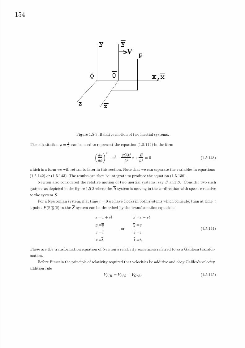
8/6/2019 Introduction to Tensor Calculus Continuum Mechanics - J. Heinbockel
http://slidepdf.com/reader/full/introduction-to-tensor-calculus-continuum-mechanics-j-heinbockel 159/372
154
Figure 1.5-3. Relative motion of two inertial systems.
The substitution ρ = 1u can be used to represent the equation (1.5.142) in the form
du
dφ
2
+ u2 − 2GM
h2u +
E
h2= 0 (1.5.143)
which is a form we will return to later in this section. Note that we can separate the variables in equations
(1.5.142) or (1.5.143). The results can then be integrate to produce the equation (1.5.130).
Newton also considered the relative motion of two inertial systems, say S and S . Consider two suchsystems as depicted in the figure 1.5-3 where the S system is moving in the x−direction with speed v relative
to the system S.
For a Newtonian system, if at time t = 0 we have clocks in both systems which coincide, than at time t
a point P (x, y, z) in the S system can be described by the transformation equations
x =x + vt
y =y
z =z
t =t
or
x =x − vt
y =y
z =z
t =t.
(1.5.144)
These are the transformation equation of Newton’s relativity sometimes referred to as a Galilean transfor-
mation.
Before Einstein the principle of relativity required that velocities be additive and obey Galileo’s velocity
addition rule
V P/R = V P/Q + V Q/R. (1.5.145)
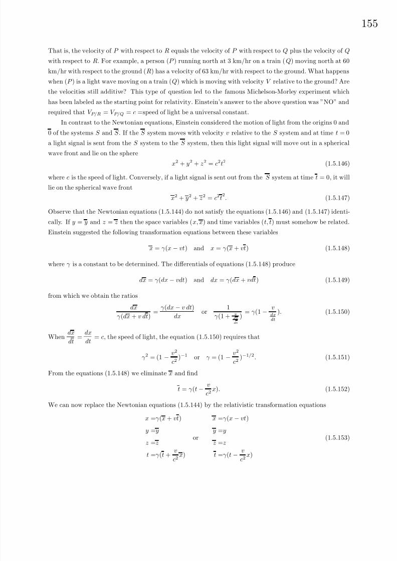
8/6/2019 Introduction to Tensor Calculus Continuum Mechanics - J. Heinbockel
http://slidepdf.com/reader/full/introduction-to-tensor-calculus-continuum-mechanics-j-heinbockel 160/372

8/6/2019 Introduction to Tensor Calculus Continuum Mechanics - J. Heinbockel
http://slidepdf.com/reader/full/introduction-to-tensor-calculus-continuum-mechanics-j-heinbockel 161/372
156
where γ is given by equation (1.5.151). These equations are also known as the Lorentz transformation.
Note that for v << c, thenv
c2≈ 0, γ ≈ 1 , then the equations (1.5.153) closely approximate the equations
(1.5.144). The equations (1.5.153) also satisfy the equations (1.5.146) and (1.5.147) identically as can be
readily verified by substitution. Further, by using chain rule differentiation we obtain from the relations
(1.5.148) that
dx
dt=
dxdt + v
1 +dx
dt
cvc
. (1.5.154)
The equation (1.5.154) is the Einstein relative velocity addition rule which replaces the previous Newtonian
rule given by equation (1.5.145). We can rewrite equation (1.5.154) in the notation of equation (1.5.145) as
V P/R =V P/Q + V Q/R
1 +V P/Q
c
V Q/R
c
. (1.5.155)
Observe that when V P/Q << c and V Q/R << c then equation (1.5.155) approximates closely the equation
(1.5.145). Also as V P/Q and V Q/R approach the speed of light we have
limV P/Q→C
V Q/R→C
V P/Q + V Q/R
1 +V P/Q
c
V Q/R
c
= c (1.5.156)
which agrees with Einstein’s hypothesis that the speed of light is an invariant.
Let us return now to the viewpoint of what gravitation is. Einstein thought of space and time as being
related and viewed the motion of the planets as being that of geodesic paths in a space-time continuum.
Recall the equations of geodesics are given by
d2xi
ds2+
i
j k
dxj
ds
dxk
ds= 0, (1.5.157)
where s is arc length. These equations are to be associated with a 4-dimensional space-time metric gij
where the indices i, j take on the values 1, 2, 3, 4 and the xi are generalized coordinates. Einstein asked
the question, ”Can one introduce a space-time metric gij such that the equations (1.5.157) can somehow
reproduce the law of gravitational attraction d2 ρdt2 + GM
ρ3 ρ = 0?” Then the motion of the planets can be
viewed as optimized motion in a space-time continuum where the metrices of the space simulate the law of
gravitational attraction. Einstein thought that this motion should be related to the curvature of the space
which can be obtained from the Riemann-Christoffel tensor Rijkl . The metric we desire gij, i, j = 1, 2, 3, 4
has 16 components. The conjugate metric tensor gij is defined such that gijgjk = δik and an element of
arc length squared is given by ds2 = gij dxidxj . Einstein thought that the metrices should come from the
Riemann-Christoffel curvature tensor which, for n = 4 has 256 components, but only 20 of these are linearly
independent. This seems like a large number of equations from which to obtain the law of gravitational
attraction and so Einstein considered the contracted tensor
Gij = Rtijt =
∂
∂xj
n
i n
− ∂
∂xn
n
i j
+
m
i n
n
m j
−
m
i j
n
m n
. (1.5.158)
Spherical coordinates (ρ,θ,φ) suggests a metric similar to
ds2 = −(dρ)2 − ρ2(dθ)2 − ρ2 sin2 θ(dφ)2 + c2(dt)2
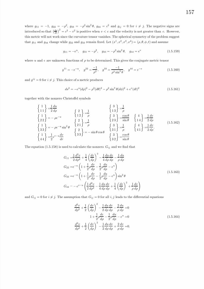
8/6/2019 Introduction to Tensor Calculus Continuum Mechanics - J. Heinbockel
http://slidepdf.com/reader/full/introduction-to-tensor-calculus-continuum-mechanics-j-heinbockel 162/372
15
where g11 = −1, g22 = −ρ2, g33 = −ρ2 sin2 θ, g44 = c2 and gij = 0 for i = j. The negative signs are
introduced so that
dsdt
2= c2 − v2 is positive when v < c and the velocity is not greater than c. However,
this metric will not work since the curvature tensor vanishes. The spherical symmetry of the problem suggest
that g11 and g44 change while g22 and g33 remain fixed. Let (x1, x2, x3, x4) = (ρ,θ,φ,t) and assume
g11 = −eu, g22 = −ρ2, g33 = −ρ2 sin2 θ, g44 = ev (1.5.159)
where u and v are unknown functions of ρ to be determined. This gives the conjugate metric tensor
g11 = −e−u, g22 =−1
ρ2, g33 =
−1
ρ2 sin2 θ, g44 = e−v (1.5.160)
and gij = 0 for i = j. This choice of a metric produces
ds2 = −eu(dρ)2 − ρ2(dθ)2 − ρ2 sin2 θ(dφ)2 + ev(dt)2 (1.5.161)
together with the nonzero Christoffel symbols1
1 1
=
1
2
du
dρ1
2 2
=− ρe−u
1
3 3
=− ρe−u sin2 θ
1
4 4
=
1
2ev−u dv
dr
2
1 2
=
1
ρ2
2 1
=
1
ρ2
3 3
=− sin θ cos θ
3
1 3
=
1
ρ3
2 3
=
cos θ
sin θ3
3 1
=
1
ρ3
3 2
=
cos θ
sin θ
4
1 4
=
1
2
dv
dρ4
4 1
=
1
2
dv
dρ.
(1.5.162)
The equation (1.5.158) is used to calculate the nonzero Gij and we find that
G11 =1
2
d2v
dρ2+
1
4
dv
dρ
2
− 1
4
du
dρ
dv
dρ− 1
ρ
du
dρ
G22 =e−u
1 +
1
2ρ
dv
dρ− 1
2ρ
du
dρ− eu
G33 =e−u
1 +
1
2ρ
dv
dρ− 1
2ρ
du
dρ− eu
sin2 θ
G44 = − ev−u
1
2
d2v
dρ2− 1
4
du
dρ
dv
dρ+
1
4
dv
dρ
2
+1
ρ
dv
dρ
(1.5.163)
and Gij = 0 for i = j. The assumption that Gij = 0 for all i, j leads to the differential equations
d2v
dρ2+
1
2
dv
dρ
2
− 1
2
du
dρ
dv
dρ− 2
ρ
du
dρ=0
1 +1
2ρ
dv
dρ− 1
2ρ
du
dρ− eu =0
d2v
dρ2+
1
2
dv
dρ
2
− 1
2
du
dρ
dv
dρ+
2
ρ
dv
dρ=0.
(1.5.164)

8/6/2019 Introduction to Tensor Calculus Continuum Mechanics - J. Heinbockel
http://slidepdf.com/reader/full/introduction-to-tensor-calculus-continuum-mechanics-j-heinbockel 163/372
158
Subtracting the first equation from the third equation gives
du
dρ+
dv
dρ= 0 or u + v = c1 = constant. (1.5.165)
The second equation in (1.5.164) then becomes
ρdudρ
= 1 − eu (1.5.166)
Separate the variables in equation (1.5.166) and integrate to obtain the result
eu =1
1 − c2ρ
(1.5.167)
where c2 is a constant of integration and consequently
ev = ec1−u = ec1
1 − c2
ρ
. (1.5.168)
The constant c1 is selected such that g44 approaches c2 as ρ increases without bound. This produces the
metrices
g11 =−1
1 − c2ρ
, g22 = −ρ2, g33 = −ρ2 sin2 θ, g44 = c2(1− c2ρ
) (1.5.169)
where c2 is a constant still to be determined. The metrices given by equation (1.5.169) are now used to
expand the equations (1.5.157) representing the geodesics in this four dimensional space. The differential
equations representing the geodesics are found to be
d2ρ
ds2+
1
2
du
dρ
dρ
ds
2− ρe−u
dθ
ds
2− ρe−u sin2 θ
dφ
ds
2+
1
2ev−u
dv
dρ
dt
ds
2= 0 (1.5.170)
d2θ
ds2
+2
ρ
dθ
ds
dρ
ds
− sin θ cos θdφ
ds2
= 0 (1.5.171)
d2φ
ds2+
2
ρ
dφ
ds
dρ
ds+ 2
cos θ
sin θ
dφ
ds
dθ
ds= 0 (1.5.172)
d2t
ds2+
dv
dρ
dt
ds
dρ
ds= 0. (1.5.173)
The equation (1.5.171) is identically satisfied if we examine planar orbits where θ = π2 is a constant. This
value of θ also simplifies the equations (1.5.170) and (1.5.172). The equation (1.5.172) becomes an exact
differential equationd
ds
ρ2
dφ
ds
= 0 or ρ2
dφ
ds= c4, (1.5.174)
and the equation (1.5.173) also becomes an exact differential
d
ds
dt
dsev
= 0 ordt
dsev = c5, (1.5.175)
where c4 and c5 are constants of integration. This leaves the equation (1.5.170) which determines ρ. Substi-
tuting the results from equations (1.5.174) and (1.5.175), together with the relation (1.5.161), the equation
(1.5.170) reduces tod2ρ
ds2+
c22ρ2
+c2c242ρ4
− (1− c2ρ
)c24ρ3
= 0. (1.5.176)

8/6/2019 Introduction to Tensor Calculus Continuum Mechanics - J. Heinbockel
http://slidepdf.com/reader/full/introduction-to-tensor-calculus-continuum-mechanics-j-heinbockel 164/372
15
By the chain rule we have
d2ρ
ds2=
d2ρ
dφ2
dφ
ds
2
+dρ
dφ
d2φ
ds2=
d2ρ
dφ2
c24ρ4
+
dρ
dφ
2−2c24ρ5
and so equation (1.5.176) can be written in the form
d2ρ
dφ2− 2
ρ
dρ
dφ
2
+c22
ρ2
c24+
c22−
1 − c2ρ
ρ = 0. (1.5.177)
The substitution ρ = 1u reduces the equation (1.5.177) to the form
d2u
dφ2+ u − c2
2c24=
3
2c2u2. (1.5.178)
Multiply the equation (1.5.178) by 2 dudφ and integrate with respect to φ to obtain
du
dφ
2
+ u2 − c2c24
u = c2u3 + c6. (1.5.179)
where c6 is a constant of integration. To determine the constant c6 we write the equation (1.5.161) in the
special case θ = π2 and use the substitutions from the equations (1.5.174) and (1.5.175) to obtain
eu
dρ
ds
2
= eu
dρ
dφ
dφ
ds
2
= 1 − ρ2
dφ
ds
2
+ ev
dt
ds
2
or dρ
dφ
2
+
1 − c2
ρ
ρ2 +
1 − c2
ρ− c25
c2
ρ4
c24= 0. (1.5.180)
The substitution ρ = 1u reduces the equation (1.5.180) to the form
dudφ2
+ u2 − c2u3 + 1c24− c2c24
u − c
2
5c2c24
= 0. (1.5.181)
Now comparing the equations (1.5.181) and (1.5.179) we select
c6 =
c25c2− 1
1
c24
so that the equation (1.5.179) takes on the formdu
dφ
2
+ u2 − c2c24
u +
1 − c25
c2
1
c24= c2u3 (1.5.182)
Now we can compare our relativistic equation (1.5.182) with our Newtonian equation (1.5.143). In order
that the two equations almost agree we select the constants c2, c4, c5 so that
c2c24
=2GM
h2and
1 − c25c2
c24=
E
h2. (1.5.183)
The equations (1.5.183) are only two equations in three unknowns and so we use the additional equation
limρ→∞
ρ2dφ
dt= lim
ρ→∞ρ2
dφ
ds
ds
dt= h (1.5.184)

8/6/2019 Introduction to Tensor Calculus Continuum Mechanics - J. Heinbockel
http://slidepdf.com/reader/full/introduction-to-tensor-calculus-continuum-mechanics-j-heinbockel 165/372
160
which is obtained from equation (1.5.141). Substituting equations (1.5.174) and (1.5.175) into equation
(1.5.184), rearranging terms and taking the limit we find that
c4c2
c5= h. (1.5.185)
From equations (1.5.183) and (1.5.185) we obtain the results that
c25 =c2
1 + Ec2
, c2 =2GM
c2
1
1 + E/c2
, c4 =
h
c
1 + E/c2(1.5.186)
These values substituted into equation (1.5.181) produce the differential equationdu
dφ
2
+ u2 − 2GM
h2u +
E
h2=
2GM
c2
1
1 + E/c2
u3. (1.5.187)
Let α = c2c24
= 2GM h2 and β = c2 = 2GM
c2 ( 11+E/c2 ) then the differential equation (1.5.178) can be written as
d2u
dφ2 + u −α
2 =3
2 βu2. (1.5.188)
We know the solution to equation (1.5.143) is given by
u =1
ρ= A(1 + cos(φ − φ0)) (1.5.189)
and so we assume a solution to equation (1.5.188) of this same general form. We know that A is small and so
we make the assumption that the solution of equation (1.5.188) given by equation (1.5.189) is such that φ0 is
approximately constant and varies slowly as a function of Aφ. Observe that if φ0 = φ0(Aφ), then dφ0
dφ = φ0A
and d2φ0
dφ2 = φ0A2, where primes denote differentiation with respect to the argument of the function. (i.e.
Aφ for this problem.) The derivatives of equation (1.5.189) producedu
dφ=− A sin(φ − φ0)(1 − φ0A)
d2u
dφ2=A3 sin(φ − φ0)φ0 − A cos(φ − φ0)(1− 2Aφ0 + A2(φ0)2)
=− A cos(φ − φ0) + 2A2φ0 cos(φ − φ0) + O(A3).
Substituting these derivatives into the differential equation (1.5.188) produces the equations
2A2φ0 cos(φ − φ0) + A − α
2=
3β
2
A2 + 2A2 cos(φ − φ0) + 2A2 cos2(φ − φ0)
+ O(A3).
Now A is small so that terms O(A3
) can be neglected. Equating the constant terms and the coefficient of the cos(φ − φ0) terms we obtain the equations
A − α
2=
3β
2A2 2A2φ0 = 3βA2 +
3β
22A2 cos(φ − φ0).
Treating φ0 as essentially constant, the above system has the approximate solutions
A ≈ α
2φ0 ≈ 3β
2Aφ +
3β
4A sin(φ − φ0) (1.5.190)
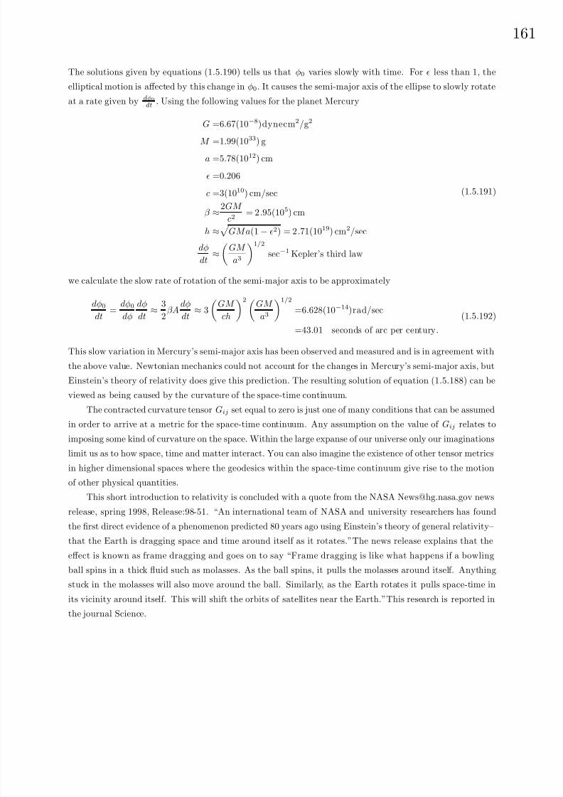
8/6/2019 Introduction to Tensor Calculus Continuum Mechanics - J. Heinbockel
http://slidepdf.com/reader/full/introduction-to-tensor-calculus-continuum-mechanics-j-heinbockel 166/372
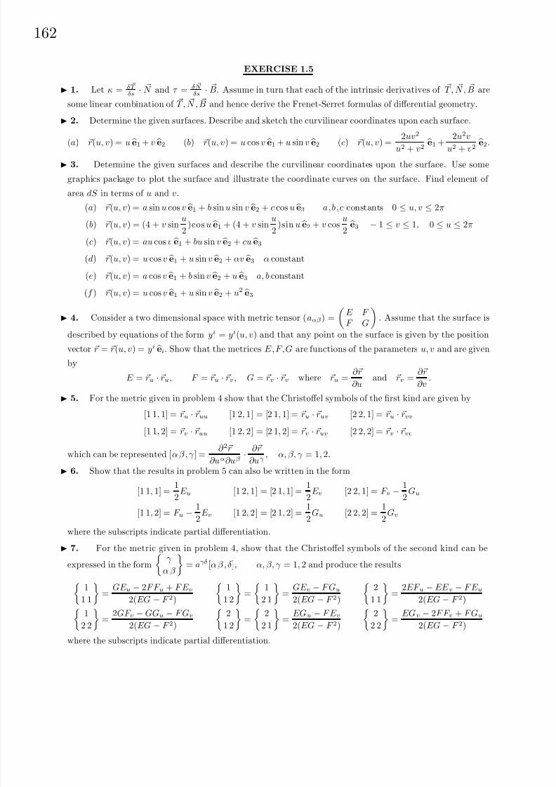
8/6/2019 Introduction to Tensor Calculus Continuum Mechanics - J. Heinbockel
http://slidepdf.com/reader/full/introduction-to-tensor-calculus-continuum-mechanics-j-heinbockel 167/372

8/6/2019 Introduction to Tensor Calculus Continuum Mechanics - J. Heinbockel
http://slidepdf.com/reader/full/introduction-to-tensor-calculus-continuum-mechanics-j-heinbockel 168/372
16
8. Derive the Gauss equations by assuming that
ruu = c1ru + c2rv + c3 n, ruv = c4ru + c5rv + c6 n, rvv = c7ru + c8rv + c9 nwhere c1, . . . , c9 are constants determined by taking dot products of the above vectors with the vectors ru, rv ,
and n. Show that c1 = 1
1 1, c2 = 2
1 1, c3 = e, c4 = 1
1 2, c5 = 2
1 2, c6 = f,
c7 =
1
2 2
, c8 =
2
2 2
, c9 = g Show the Gauss equations can be written
∂ 2r
∂uα∂uβ=
γ
α β
∂r
∂uγ+ bαβ n.
9. Derive the Weingarten equations
nu = c1ru + c2rv nv = c3ru + c4rv
andru = c∗1 nu + c∗2 nv
rv = c∗3 nu + c∗4 nv
and show
c1 =f F − eG
EG − F 2
c2 =eF
−f E
EG − F 2
c3 =gF − f G
EG − F 2
c4 =f F
−gE
EG − F 2
c∗1 =f F − gE
eg − f 2
c∗
2 =f E
−eF
eg − f 2
c∗3 =f G − gF
eg − f 2
c∗
4 =f F
−eG
eg − f 2
The constants in the above equations are determined in a manner similar to that suggested in problem 8.
Show that the Weingarten equations can be written in the form
∂ n∂uα
= −bβα
∂r
∂uβ.
10. Using n =ru × rv√EG − F 2
, the results from exercise 1.1, problem 9(a), and the results from problem 5,
verify that
(ru × ruu) · n = 2
1 1 EG − F 2
(ru × ruv) · n =
2
1 2
EG − F 2
(rv × ruu) · n = −
1
1 1
EG − F 2
(ru × rvv ) · n =
2
2 2
EG − F 2
(rv × ruv ) · n = −
1
2 1
EG − F 2
(rv × rvv ) · n = −
1
2 2
EG − F 2
(ru × rv) · n =
EG − F 2
and then derive the formula for the geodesic curvature given by equation (1.5.48).
Hint:(
n × T ) · d T
ds= ( T × d T
ds) ·
n and aαδ]β γ , δ] =
α
β γ .

8/6/2019 Introduction to Tensor Calculus Continuum Mechanics - J. Heinbockel
http://slidepdf.com/reader/full/introduction-to-tensor-calculus-continuum-mechanics-j-heinbockel 169/372

8/6/2019 Introduction to Tensor Calculus Continuum Mechanics - J. Heinbockel
http://slidepdf.com/reader/full/introduction-to-tensor-calculus-continuum-mechanics-j-heinbockel 170/372
16
20. Find the number of independent components associated with the Riemann Christoffel tensor
Rijkm, i, j, k, m = 1, 2, . . . , N . There are N 4 components to examine in an N −dimensional space. Many of
these components are zero and many of the nonzero components are related to one another by symmetries
or the cyclic properties. Verify the following cases:
CASE I We examine components of the form Rinin , i
= n with no summation of i or n. The first index
can be chosen in N ways and therefore with i = n the second index can be chosen in N − 1 ways. Observe
that Rinin = Rnini, (no summation on i or n) and so one half of the total combinations are repeated. This
leaves M 1 = 12N (N − 1) components of the form Rinin. The quantity M 1 can also be thought of as the
number of distinct pairs of indices (i, n).
CASE II We next examine components of the form Rinji, i = n = j where there is no summation on
the index i. We have previously shown that the first pair of indices can be chosen in M 1 ways. Therefore,
the third index can be selected in N − 2 ways and consequently there are M 2 = 12N (N − 1)(N − 2) distinct
components of the form Rinji with i = n = j.
CASE III Next examine components of the form Rinjk where i = n = j = k. From CASE I the first pairs
of indices (i, n) can be chosen in M 1 ways. Taking into account symmetries, it can be shown that the secondpair of indices can be chosen in 1
2(N −2)(N −3) ways. This implies that there are 14N (N −1)(N −2)(N −3)
ways of choosing the indices i,n,j and k with i = n = j = k. By symmetry the pairs (i, n) and ( j,k) can be
interchanged and therefore only one half of these combinations are distinct. This leaves
1
8N (N − 1)(N − 2)(N − 3)
distinct pairs of indices. Also from the cyclic relations we find that only two thirds of the above components
are distinct. This produces
M 3 =N (N − 1)(N − 2)(N − 3)
12
distinct components of the form Rinjk with i = n = j = k.Adding the above components from each case we find there are
M 4 = M 1 + M 2 + M 3 =N 2(N 2 − 1)
12
distinct and independent components.
Verify the entries in the following table:
Dimension of space N 1 2 3 4 5
Number of components N 4 1 16 81 256 625
M 4 = Independent components of Rijkm 0 1 6 20 50
Note 1: A one dimensional space can not be curved and all one dimensional spaces are Euclidean. (i.e. if we have
an element of arc length squared given by ds2 = f (x)(dx)2, we can make the coordinate transformation f (x)dx = du and reduce the arc length squared to the form ds2 = du2.)
Note 2: In a two dimensional space, the indices can only take on the values 1 and 2. In this special case there
are 16 possible components. It can be shown that the only nonvanishing components are:
R1212 = −R1221 = −R2112 = R2121.
8/6/2019 Introduction to Tensor Calculus Continuum Mechanics - J. Heinbockel
http://slidepdf.com/reader/full/introduction-to-tensor-calculus-continuum-mechanics-j-heinbockel 171/372
166
For these nonvanishing components only one independent component exists. By convention, the com-
ponent R1212 is selected as the single independent component and all other nonzero components are
expressed in terms of this component.
Find the nonvanishing independent components Rijkl for i, j, k, l = 1, 2, 3, 4 and show that
R1212
R1313
R2323
R1414
R2424
R3434
R1231
R1421
R1341
R2132
R2142
R2342
R3213
R3243
R3143
R4124
R4314
R4234
R1324
R1432
can be selected as the twenty independent components.
21.
(a) For N = 2 show R1212 is the only nonzero independent component and
R1212 = R2121 = −R1221 = −R2112.(b) Show that on the surface of a sphere of radius r0 we have R1212 = r20 sin2 θ.
22. Show for N = 2 that
R1212 = R1212J 2 = R1212
∂x
∂x
2 23. Define Rij = Rs
.ijs as the Ricci tensor and Gij = Ri
j − 12δi
j R as the Einstein tensor, where Rij = gikRkj
and R = Rii. Show that
(a) Rjk = gabRjabk
(b) Rij =∂ 2 log
√g
∂xi∂xj−
b
i j∂ log
√g
∂xb− ∂
∂xaa
i j+
b
i aa
j b(c) Riijk = 0
24. By employing the results from the previous problem show that in the case N = 2 we have
R11
g11=
R22
g22=
R12
g12= −R1212
g
where g is the determinant of gij.
25. Consider the case N = 2 where we have g12 = g21 = 0 and show that
(a) R12 = R21 = 0
(b) R11g22 = R22g11 = R1221
(c) R =2R1221
g11g22
(d) Rij = 12
Rgij, where R = gijRij
The scalar invariant R is known as the Einstein curvature of the surface and the tensor Gij = Ri
j − 12δi
j R is
known as the Einstein tensor.
26. For N = 3 show that R1212, R1313, R2323, R1213, R2123, R3132 are independent components of the
Riemann Christoffel tensor.
8/6/2019 Introduction to Tensor Calculus Continuum Mechanics - J. Heinbockel
http://slidepdf.com/reader/full/introduction-to-tensor-calculus-continuum-mechanics-j-heinbockel 172/372
16
27. For N = 2 and aαβ =
a11 0
0 a22
show that
K =R1212
a= − 1
2√
a
∂
∂u1
1√a
∂a22
∂u1
+
∂
∂u2
1√
a
∂a11
∂u2
.
28. For N = 2 and aαβ = a11 a12a21 a22
show that
K =1
2√
a
∂
∂u1
a12
a11√
a
∂a11
∂u2− 1√
a
∂a22
∂u1
+
∂
∂u2
2√
a
∂a12
∂u1− 1√
a
∂a11
∂u2− a12
a11√
a
∂a11
∂u1
.
Check your results by setting a12 = a21 = 0 and comparing this answer with that given in the problem 27.
29. Write out the Frenet-Serret formulas (1.5.112)(1.5.113) for surface curves in terms of Christoffel
symbols of the second kind.
30.
(a) Use the fact that for n = 2 we have R1212 = R2121 = −R2112 = −R1221 together with eαβ, eαβ the two
dimensional alternating tensors to show that the equation (1.5.110) can be written as
Rαβγδ = Kαβγδ where αβ =√
aeαβ and αβ =1√a
eαβ
are the corresponding epsilon tensors.
(b) Show that from the result in part (a) we obtain1
4Rαβγδαβγδ = K.
Hint: See equations (1.3.82),(1.5.93) and (1.5.94).
31. Verify the result given by the equation (1.5.100).
32. Show that aαβcαβ = 4H 2 − 2K.
33. Find equations for the principal curvatures associated with the surface
x = u, y = v, z = f (u, v).
34. Geodesics on a sphere Let (θ, φ) denote the surface coordinates of the sphere of radius ρ defined
by the parametric equations
x = ρ sin θ cos φ, y = ρ sin θ sin φ, z = ρ cos θ. (1)
Consider also a plane which passes through the origin with normal having the direction numbers (n1, n2, n3).
This plane is represented by n1x + n2y + n3z = 0 and intersects the sphere in a great circle which is described
by the relation
n1 sin θ cos φ + n2 sin θ sin φ + n3 cos θ = 0. (2)
This is an implicit relation between the surface coordinates θ, φ which describes the great circle lying on the
sphere. We can write this later equation in the form
n1 cos φ + n2 sin φ =−n3
tan θ(3)

8/6/2019 Introduction to Tensor Calculus Continuum Mechanics - J. Heinbockel
http://slidepdf.com/reader/full/introduction-to-tensor-calculus-continuum-mechanics-j-heinbockel 173/372
168
and in the special case where n1 = cos β , n2 = sin β ,n3 = − tan α is expressible in the form
cos(φ − β ) =tan α
tan θor φ − β = cos−1
tan α
tan θ
. (4)
The above equation defines an explicit relationship between the surface coordinates which defines a great
circle on the sphere. The arc length squared relation satisfied by the surface coordinates together with theequation obtained by differentiating equation (4) with respect to arc length s gives the relations
sin2 θdφ
ds=
tan α 1 − tan2 α
tan2 θ
dθ
ds(5)
ds2 = ρ2 dθ2 + ρ2 sin2 θ dφ2 (6)
The above equations (1)-(6) are needed to consider the following problem.
(a) Show that the differential equations defining the geodesics on the surface of a sphere (equations (1.5.51))
ared2θ
ds2− sin θ cos θ
dφ
ds
2
= 0 (7)
d2φ
ds2+ 2 cot θ
dθ
ds
dφ
ds= 0 (8)
(b) Multiply equation (8) by sin2 θ and integrate to obtain
sin2 θdφ
ds= c1 (9)
where c1 is a constant of integration.
(c) Multiply equation (7) by dθds and use the result of equation (9) to show that an integration produces
dθ
ds
2
=−c21
sin2 θ+ c22 (10)
where c22 is a constant of integration.
(d) Use the equations (5)(6) to show that c2 = 1/ρ and c1 = sinαρ .
(e) Show that equations (9) and (10) imply that
dφ
dθ =tan α
tan2 θ
sec2 θ 1− tan2 α
tan2 θ
and making the substitution u = tan αtan θ this equation can be integrated to obtain the equation (4). We
can now expand the equation (4) and express the results in terms of x, y, z to obtain the equation (3).
This produces a plane which intersects the sphere in a great circle. Consequently, the geodesics on a
sphere are great circles.
8/6/2019 Introduction to Tensor Calculus Continuum Mechanics - J. Heinbockel
http://slidepdf.com/reader/full/introduction-to-tensor-calculus-continuum-mechanics-j-heinbockel 174/372
16
35. Find the differential equations defining the geodesics on the surface of a cylinder.
36. Find the differential equations defining the geodesics on the surface of a torus. (See problem 13,
Exercise 1.3)
37. Find the differential equations defining the geodesics on the surface of revolution
x = r cos φ, y = r sin φ, z = f (r).
Note the curve z = f (x) gives a profile of the surface. The curves r = Constant are the parallels, while the
curves φ = Constant are the meridians of the surface and
ds2 = (1 + f 2) dr2 + r2dφ2.
38. Find the unit normal and tangent plane to an arbitrary point on the right circular cone
x = u sin α cos φ, y = u sin α sin φ, z = u cos α.
This is a surface of revolution with r = u sin α and f (r) = r cot α with α constant.
39. Let s denote arc length and assume the position vector r(s) is analytic about a point s0. Show that
the Taylor series r(s) = r(s0) + hr (s0) +h2
2!r (s0) +
h3
3!r (s0) + · · · about the point s0, with h = s− s0 is
given by r(s) = r(s0) + h T + 12
κh2 N + 16
h3(−κ2 T + κ N + κτ B) + · · · which is obtained by differentiating
the Frenet formulas.
40.
(a) Show that the circular helix defined by x = a cos t, y = a sin t, z = bt with a, b constants, has the
property that any tangent to the curve makes a constant angle with the line defining the z-axis.
(i.e. T · e3 = cos α = constant.)
(b) Show also that N · e3 = 0 and consequently e3 is parallel to the rectifying plane, which implies that e3 = T cos α + B sin α.
(c) Differentiate the result in part (b) and show that κ/τ = tan α is a constant.
41. Consider a space curve xi = xi(s) in Cartesian coordinates.
(a) Show that κ =d T
ds
=
xixi
(b) Show that τ =1
κ2eijk xixj xk . Hint: Consider r · r × r
42.
(a) Find the direction cosines of a normal to a surface z = f (x, y).
(b) Find the direction cosines of a normal to a surface F (x, y, z) = 0.
(c) Find the direction cosines of a normal to a surface x = x(u, v), y = y(u, v), z = z(u, v).
43. Show that for a smooth surface z = f (x, y) the Gaussian curvature at a point on the surface is given
by
K =f xxf yy − f 2xy
(f 2x + f 2y + 1)2.

8/6/2019 Introduction to Tensor Calculus Continuum Mechanics - J. Heinbockel
http://slidepdf.com/reader/full/introduction-to-tensor-calculus-continuum-mechanics-j-heinbockel 175/372
170
44. Show that for a smooth surface z = f (x, y) the mean curvature at a point on the surface is given by
H =(1 + f 2y )f xx − 2f xf yf xy + (1 + f 2x )f yy
2(f 2x + f 2y + 1)3/2.
45. Express the Frenet-Serret formulas (1.5.13) in terms of Christoffel symbols of the second kind.
46. Verify the relation (1.5.106).
47. In V n assume that Rij = ρgij and show that ρ = Rn where R = gijRij . This result is known as
Einstein’s gravitational equation at points where matter is present. It is analogous to the Poisson equation
∇2V = ρ from the Newtonian theory of gravitation.
48. In V n assume that Rijkl = K (gikgjl − gilgjk ) and show that R = Kn(1− n). (Hint: See problem 23.)
49. Assume gij = 0 for i = j and verify the following.
(a) Rhijk = 0 for h = i = j = k
(b) Rhiik =√
gii
∂ 2√
gii
∂xh∂xk− ∂
√gii
∂xh
∂ log√
ghh
∂xk− ∂
√gii
∂xk
∂ log√
gkk
∂xh
for h,i,k unequal.
(c) Rhiih =√
gii√
ghh
∂
∂xh
1√ghh
∂ √gii
∂xh
+
∂
∂xi
1√gii
∂ √ghh
∂xi
+
nm=1
m=h m=i
∂ √gii
∂xm
∂ √ghh
∂xm
where h = i.
50. Consider a surface of revolution where x = r cos θ, y = r sin θ and z = f (r) is a given function of r.
(a) Show in this V 2 we have ds2 = (1 + (f )2)dr2 + r2dθ2 where = dds .
(b) Show the geodesic equations in this V 2 are
d2r
ds2+
f f
1 + (f )2
dr
ds
2
− r
1 + (f )2
dθ
ds
2
= 0
d2θ
ds2+
2
r
dθ
ds
dr
ds= 0
(c) Solve the second equation in part (b) to obtaindθ
ds=
a
r2. Substitute this result for ds in part (a) to show
dθ = ±a
1 + (f )2
r√
r2 − a2dr which theoretically can be integrated.

8/6/2019 Introduction to Tensor Calculus Continuum Mechanics - J. Heinbockel
http://slidepdf.com/reader/full/introduction-to-tensor-calculus-continuum-mechanics-j-heinbockel 176/372
17
PART 2: INTRODUCTION TO CONTINUUM MECHANICS
In the following sections we develop some applications of tensor calculus in the areas of dynamics,
elasticity, fluids and electricity and magnetism. We begin by first developing generalized expressions for the
vector operations of gradient, divergence, and curl. Also generalized expressions for other vector operators
are considered in order that tensor equations can be converted to vector equations. We construct a table to
aid in the translating of generalized tensor equations to vector form and vice versa.
The basic equations of continuum mechanics are developed in the later sections. These equations are
developed in both Cartesian and generalized tensor form and then converted to vector form.
§2.1 TENSOR NOTATION FOR SCALAR AND VECTOR QUANTITIES
We consider the tensor representation of some vector expressions. Our goal is to develop the ability to
convert vector equations to tensor form as well as being able to represent tensor equations in vector form.
In this section the basic equations of continuum mechanics are represented using both a vector notation andthe indicial notation which focuses attention on the tensor components. In order to move back and forth
between these notations, the representation of vector quantities in tensor form is now considered.
Gradient
For Φ = Φ(x1, x2, . . . , xN ) a scalar function of the coordinates xi, i = 1, . . . , N , the gradient of Φ is
defined as the covariant vector
Φ,i =∂ Φ
∂xi, i = 1, . . . , N . (2.1.1)
The contravariant form of the gradient is
g
im
Φ,m. (2.1.2)
Note, if C i = gimΦ,m, i = 1, 2, 3 are the tensor components of the gradient then in an orthogonal coordinate
system we will have
C 1 = g11Φ,1, C 2 = g22Φ,2, C 3 = g33Φ,3.
We note that in an orthogonal coordinate system that gii = 1/h2i , (no sum on i), i = 1, 2, 3 and hence
replacing the tensor components by their equivalent physical components there results the equations
C (1)
h1=
1
h21
∂ Φ
∂x1,
C (2)
h2=
1
h22
∂ Φ
∂x2,
C (3)
h3=
1
h23
∂ Φ
∂x3.
Simplifying, we find the physical components of the gradient are
C (1) =1
h1
∂ Φ
∂x1, C (2) =
1
h2
∂ Φ
∂x2, C (3) =
1
h3
∂ Φ
∂x3.
These results are only valid when the coordinate system is orthogonal and gij = 0 for i = j and gii = h2i ,
with i = 1, 2, 3, and where i is not summed.
8/6/2019 Introduction to Tensor Calculus Continuum Mechanics - J. Heinbockel
http://slidepdf.com/reader/full/introduction-to-tensor-calculus-continuum-mechanics-j-heinbockel 177/372
172
Divergence
The divergence of a contravariant tensor Ar is obtained by taking the covariant derivative with respect
to xk and then performing a contraction. This produces
div Ar = Ar,r. (2.1.3)
Still another form for the divergence is obtained by simplifying the expression (2.1.3). The covariant deriva-
tive can be represented
Ar,k =
∂Ar
∂xk+
r
m k
Am.
Upon contracting the indices r and k and using the result from Exercise 1.4, problem 13, we obtain
Ar,r =
∂Ar
∂xr+
1√g
∂ (√
g)
∂xmAm
Ar,r =
1√g
√g
∂Ar
∂xr+ Ar ∂
√g
∂xr Ar
,r =1√
g
∂
∂xr(√
gAr) .
(2.1.4)
EXAMPLE 2.1-1. (Divergence) Find the representation of the divergence of a vector Ar in spherical
coordinates (ρ,θ,φ). Solution: In spherical coordinates we have
x1 = ρ, x2 = θ, x3 = φ with gij = 0 for i = j and
g11 = h21 = 1, g22 = h2
2 = ρ2, g33 = h23 = ρ2 sin2 θ.
The determinant of gij is g = |gij| = ρ4 sin2 θ and√
g = ρ2 sin θ. Employing the relation (2.1.4) we find
div Ar =1√
g
∂
∂x1(√
gA1) +∂
∂x2(√
gA2) +∂
∂x3(√
gA3)
.
In terms of the physical components this equation becomes
div Ar =1√
g
∂
∂ρ(√
gA(1)
h1) +
∂
∂θ(√
gA(2)
h2) +
∂
∂φ(√
gA(3)
h3)
.
By using the notation
A(1) = Aρ, A(2) = Aθ, A(3) = Aφ
for the physical components, the divergence can be expressed in either of the forms:
div Ar =1
ρ2 sin θ
∂
∂ρ(ρ2 sin θAρ) +
∂
∂θ(ρ2 sin θ
Aθ
ρ) +
∂
∂φ(ρ2 sin θ
Aφ
ρ sin θ)
or
div Ar =1
ρ2∂
∂ρ(ρ2Aρ) +
1
ρ sin θ
∂
∂θ(sin θAθ) +
1
ρ sin θ
∂Aφ
∂φ.
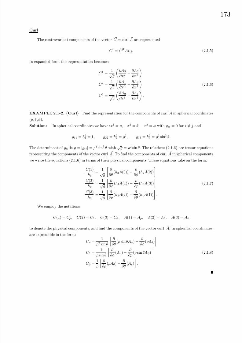
8/6/2019 Introduction to Tensor Calculus Continuum Mechanics - J. Heinbockel
http://slidepdf.com/reader/full/introduction-to-tensor-calculus-continuum-mechanics-j-heinbockel 178/372

8/6/2019 Introduction to Tensor Calculus Continuum Mechanics - J. Heinbockel
http://slidepdf.com/reader/full/introduction-to-tensor-calculus-continuum-mechanics-j-heinbockel 179/372
174
Laplacian
The Laplacian ∇2U has the contravariant form
∇2U = gijU ,ij = (gijU ,i),j =
gij
∂U
∂xi
,j
. (2.1.9)
Expanding this expression produces the equations:
∇2U =∂
∂xj
gij
∂U
∂xi
+ gim
∂U
∂xi
j
m j
∇2U =∂
∂xj
gij
∂U
∂xi
+
1√g
∂ √
g
∂xjgij
∂U
∂xi
∇2U =1√
g
√g
∂
∂xj
gij
∂U
∂xi
+ gij
∂U
∂xi
∂ √
g
∂xj
∇2U =1√
g
∂
∂xj
√ggij
∂U
∂xi
.
(2.1.10)
In orthogonal coordinates we have gij = 0 for i = j and
g11 = h21, g22 = h2
2, g33 = h23
and so (2.1.10) when expanded reduces to the form
∇2U =1
h1h2h3
∂
∂x1
h2h3
h1
∂U
∂x1
+
∂
∂x2
h1h3
h2
∂U
∂x2
+
∂
∂x3
h1h2
h3
∂U
∂x3
. (2.1.11)
This representation is only valid in an orthogonal system of coordinates.
EXAMPLE 2.1-3. (Laplacian) Find the Laplacian in spherical coordinates.
Solution: Utilizing the results given in the previous example we find the Laplacian in spherical coordinates
has the form
∇2U =1
ρ2 sin θ
∂
∂ρ
ρ2 sin θ
∂U
∂ρ
+
∂
∂θ
sin θ
∂U
∂θ
+
∂
∂φ
1
sin θ
∂U
∂φ
. (2.1.12)
This simplifies to
∇2U =∂ 2U
∂ρ2+
2
ρ
∂U
∂ρ+
1
ρ2∂ 2U
∂θ2+
cot θ
ρ2∂U
∂θ+
1
ρ2 sin2 θ
∂ 2U
∂φ2. (2.1.13)
The table 1 gives the vector and tensor representation for various quantities of interest.

8/6/2019 Introduction to Tensor Calculus Continuum Mechanics - J. Heinbockel
http://slidepdf.com/reader/full/introduction-to-tensor-calculus-continuum-mechanics-j-heinbockel 180/372
17
VECTOR GENERAL TENSOR CARTESIAN TENSOR
A A
i
or Ai Ai
A · B AiBi = gijAiBj = AiBi
AiBi = gijAiBj
AiBi
C = A × B C i =1√
geijkAjBk C i = eijkAjBk
∇Φ = grad Φ gimΦ,m Φ,i =∂ Φ
∂xi
∇ · A = div A gmnAm,n = Ar,r =
1√g
∂
∂xr(√
gAr) Ai,i =∂Ai
∂xi
∇× A = C = curl A C i = ijkAk,j C i = eijk∂Ak
∂xj
∇2U gmnU ,mn =1√
g
∂
∂xj
√ggij
∂U
∂xi
∂
∂xi
∂U
∂xi
C = ( A · ∇) B C i = AmBi,m C i = Am
∂Bi
∂xm
C = A(∇ · B) C i = AiBj,j C i = Ai
∂Bm
∂xm
C = ∇2 A C i = gjmAi,mj or C i = gjmAi,mj C i = ∂
∂xm
∂Ai
∂xm
A · ∇
φ gimAiφ ,m Aiφ,i
∇∇ · A
gim
Ar
,r
,m
∂ 2Ar
∂xi∂xr
∇×∇× A
ijkgjm
kstAt,s
,m
∂ 2Aj
∂xj∂xi− ∂ 2Ai
∂xj∂xj
Table 1 Vector and tensor representations.
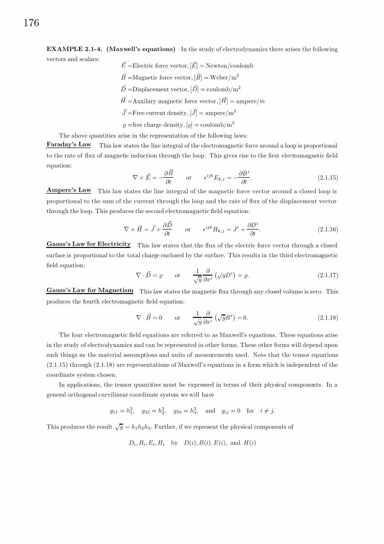
8/6/2019 Introduction to Tensor Calculus Continuum Mechanics - J. Heinbockel
http://slidepdf.com/reader/full/introduction-to-tensor-calculus-continuum-mechanics-j-heinbockel 181/372
176
EXAMPLE 2.1-4. (Maxwell’s equations) In the study of electrodynamics there arises the following
vectors and scalars: E =Electric force vector, [ E ] = Newton/coulomb
B =Magnetic force vector, [ B] = Weber/m2
D =Displacement vector, [ D] = coulomb/m2
H =Auxilary magnetic force vector, [ H ] = ampere/m
J =Free current density, [ J ] = ampere/m2
=free charge density, [] = coulomb/m3
The above quantities arise in the representation of the following laws:
Faraday’s Law This law states the line integral of the electromagnetic force around a loop is proportional
to the rate of flux of magnetic induction through the loop. This gives rise to the first electromagnetic field
equation:
∇× E = −∂ B
∂tor ijkE k,j = −∂B i
∂t. (2.1.15)
Ampere’s Law This law states the line integral of the magnetic force vector around a closed loop isproportional to the sum of the current through the loop and the rate of flux of the displacement vector
through the loop. This produces the second electromagnetic field equation:
∇× H = J +∂ D
∂tor ijkH k,j = J i +
∂Di
∂t. (2.1.16)
Gauss’s Law for Electricity This law states that the flux of the electric force vector through a closed
surface is proportional to the total charge enclosed by the surface. This results in the third electromagnetic
field equation:
∇ · D = or1√
g
∂
∂xi √
gDi
= . (2.1.17)
Gauss’s Law for Magnetism This law states the magnetic flux through any closed volume is zero. This
produces the fourth electromagnetic field equation:
∇ · B = 0 or1√
g
∂
∂xi
√gB i
= 0. (2.1.18)
The four electromagnetic field equations are referred to as Maxwell’s equations. These equations arise
in the study of electrodynamics and can be represented in other forms. These other forms will depend upon
such things as the material assumptions and units of measurements used. Note that the tensor equations
(2.1.15) through (2.1.18) are representations of Maxwell’s equations in a form which is independent of the
coordinate system chosen.
In applications, the tensor quantities must be expressed in terms of their physical components. In a
general orthogonal curvilinear coordinate system we will have
g11 = h21, g22 = h2
2, g33 = h23, and gij = 0 for i = j.
This produces the result√
g = h1h2h3. Further, if we represent the physical components of
Di, Bi, E i, H i by D(i), B(i), E (i), and H (i)

8/6/2019 Introduction to Tensor Calculus Continuum Mechanics - J. Heinbockel
http://slidepdf.com/reader/full/introduction-to-tensor-calculus-continuum-mechanics-j-heinbockel 182/372
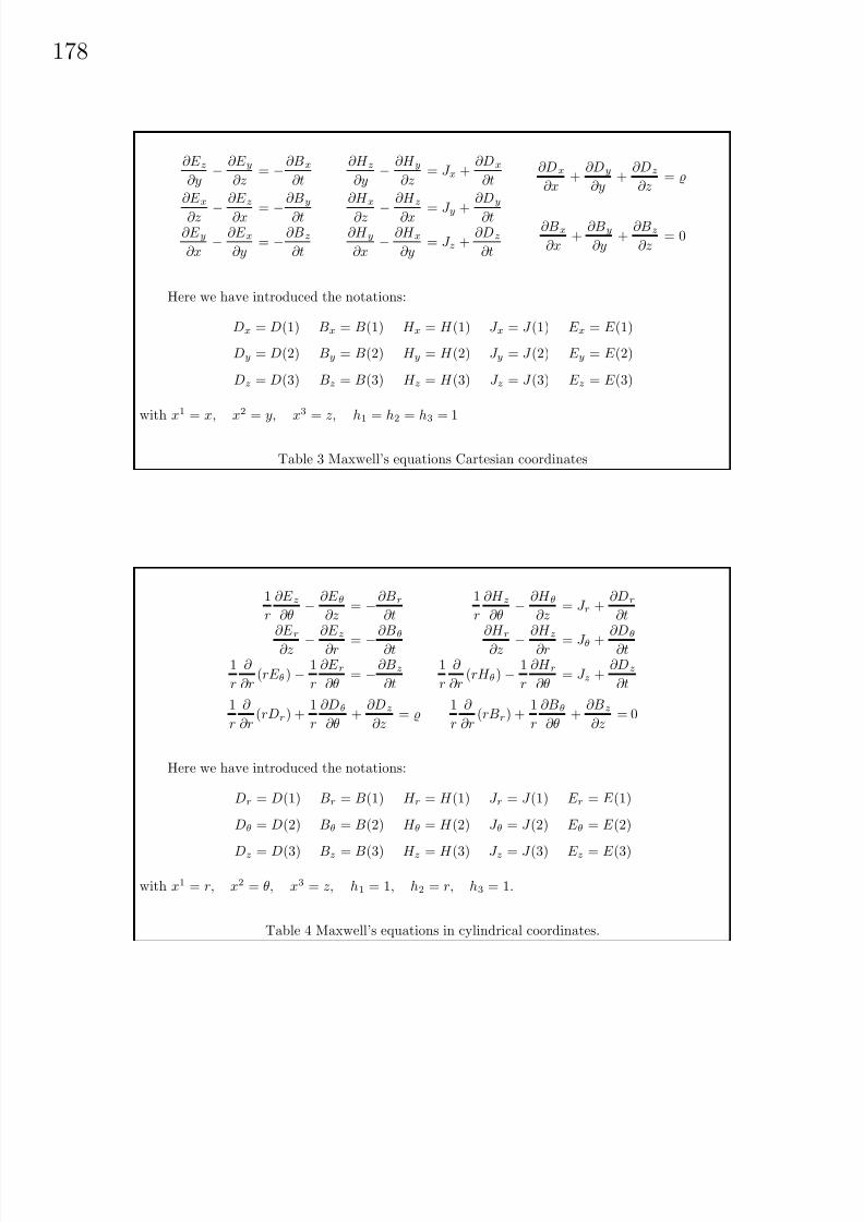
8/6/2019 Introduction to Tensor Calculus Continuum Mechanics - J. Heinbockel
http://slidepdf.com/reader/full/introduction-to-tensor-calculus-continuum-mechanics-j-heinbockel 183/372
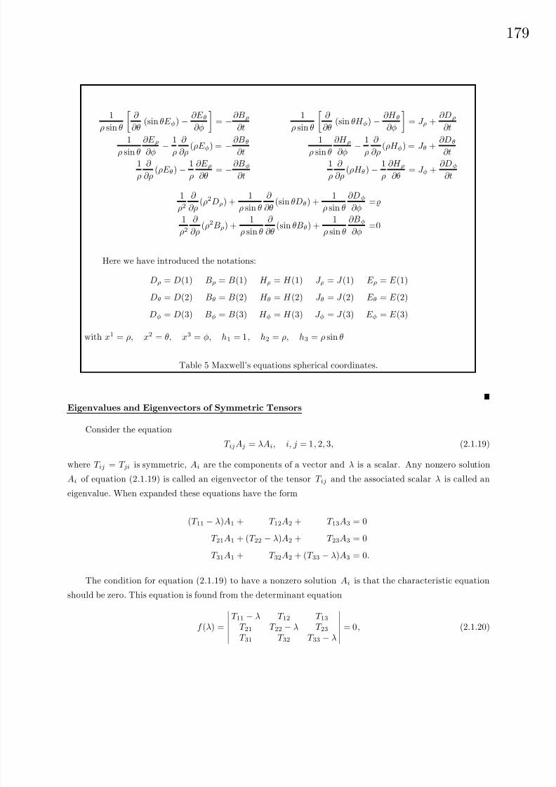
8/6/2019 Introduction to Tensor Calculus Continuum Mechanics - J. Heinbockel
http://slidepdf.com/reader/full/introduction-to-tensor-calculus-continuum-mechanics-j-heinbockel 184/372

8/6/2019 Introduction to Tensor Calculus Continuum Mechanics - J. Heinbockel
http://slidepdf.com/reader/full/introduction-to-tensor-calculus-continuum-mechanics-j-heinbockel 185/372
180
which when expanded is a cubic equation of the form
f (λ) = −λ3 + I 1λ2 − I 2λ + I 3 = 0, (2.1.21)
where I 1, I 2 and I 3 are invariants defined by the relations
I 1 = T ii
I 2 =1
2T iiT jj − 1
2T ijT ij
I 3 = eijkT i1T j2T k3.
(2.1.22)
When T ij is subjected to an orthogonal transformation, where T mn = T ijimjn, then
imjn (T mn − λ δmn) = T ij − λ δij and det (T mn − λ δmn) = det
T ij − λ δij
.
Hence, the eigenvalues of a second order tensor remain invariant under an orthogonal transformation.
If T ij is real and symmetric then
• the eigenvalues of T ij will be real, and
• the eigenvectors corresponding to distinct eigenvalues will be orthogonal.
Proof: To show a quantity is real we show that the conjugate of the quantity equals the given quantity. If
(2.1.19) is satisfied, we multiply by the conjugate Ai and obtain
AiT ijAj = λAiAi. (2.1.25)
The right hand side of this equation has the inner product AiAi which is real. It remains to show the left
hand side of equation (2.1.25) is also real. Consider the conjugate of this left hand side and write
AiT ijAj = AiT ijAj = AiT jiAj = AiT ijAj .
Consequently, the left hand side of equation (2.1.25) is real and the eigenvalue λ can be represented as the
ratio of two real quantities.
Assume that λ(1) and λ(2) are two distinct eigenvalues which produce the unit eigenvectors L1 and L2
with components i1 and i2, i = 1, 2, 3 respectively. We then have
T ijj1 = λ(1)i1 and T ijj2 = λ(2)i2. (2.1.26)
Consider the productsλ(1)i1i2 = T ijj1i2,
λ(2)i1i2 = i1T ijj2 = j1T jii2.(2.1.27)
and subtract these equations. We find that
[λ(1) − λ(2)]i1i2 = 0. (2.1.28)
By hypothesis, λ(1) is different from λ(2) and consequently the inner product i1i2 must be zero. Therefore,
the eigenvectors corresponding to distinct eigenvalues are orthogonal.

8/6/2019 Introduction to Tensor Calculus Continuum Mechanics - J. Heinbockel
http://slidepdf.com/reader/full/introduction-to-tensor-calculus-continuum-mechanics-j-heinbockel 186/372
18
Therefore, associated with distinct eigenvalues λ(i), i = 1, 2, 3 there are unit eigenvectors
L(i) = i1 e1 + i2 e2 + i3 e3
with components im, m = 1, 2, 3 which are direction cosines and satisfy
inim = δmn and ijjm = δim. (2.1.23)
The unit eigenvectors satisfy the relations
T ijj1 = λ(1)i1 T ijj2 = λ(2)i2 T ijj3 = λ(3)i3
and can be written as the single equation
T ijjm = λ(m)im, m = 1, 2, or 3 m not summed.
Consider the transformation
xi = ijxj or xm = mjxj
which represents a rotation of axes, where ij are the direction cosines from the eigenvectors of T ij. This is a
linear transformation where the ij satisfy equation (2.1.23). Such a transformation is called an orthogonal
transformation. In the new x coordinate system, called principal axes, we have
T mn = T ij∂xi
∂xm
∂xj
∂xn = T ijimjn = λ(n)inim = λ(n)δmn (no sum on n). (2.1.24)
This equation shows that in the barred coordinate system there are the components
T mn
=
λ(1) 0 0
0 λ(2) 00 0 λ(3)
.
That is, along the principal axes the tensor components T ij are transformed to the components T ij where
T ij = 0 for i = j. The elements T (i)(i) , i not summed, represent the eigenvalues of the transformation
(2.1.19).

8/6/2019 Introduction to Tensor Calculus Continuum Mechanics - J. Heinbockel
http://slidepdf.com/reader/full/introduction-to-tensor-calculus-continuum-mechanics-j-heinbockel 187/372
182
EXERCISE 2.1
1. In cylindrical coordinates (r,θ,z) with f = f (r,θ,z) find the gradient of f.
2. In cylindrical coordinates (r,θ,z) with A = A(r,θ,z) find div A.
3. In cylindrical coordinates (r,θ,z) for A = A(r,θ,z) find curl A.
4. In cylindrical coordinates (r,θ,z) for f = f (r,θ,z) find ∇2 f.
5. In spherical coordinates (ρ,θ,φ) with f = f (ρ,θ,φ) find the gradient of f.
6. In spherical coordinates (ρ,θ,φ) with A = A(ρ,θ,φ) find div A.
7. In spherical coordinates (ρ,θ,φ) for A = A(ρ,θ,φ) find curl A.
8. In spherical coordinates (ρ,θ,φ) for f = f (ρ,θ,φ) find ∇2 f.
9. Let r = x e1+ y e2+z e3 denote the position vector of a variable point (x, y, z) in Cartesian coordinates.
Let r = |r| denote the distance of this point from the origin. Find in terms of r and r:
(a) grad (r) (b) grad (rm) (c) grad (1
r) (d) grad(lnr) (e) grad (φ)
where φ = φ(r) is an arbitrary function of r.
10. Let r = x e1+y e2+z e3 denote the position vector of a variable point (x, y, z) in Cartesian coordinates.
Let r = |r| denote the distance of this point from the origin. Find:
(a) div (r) (b) div (rmr) (c) div (r−3r) (d) div (φ r)
where φ = φ(r) is an arbitrary function or r.
11. Let r = x e1 + y e2 + z e3 denote the position vector of a variable point (x, y, z) in Cartesian
coordinates. Let r = |r| denote the distance of this point from the origin. Find: (a) curl r (b) curl (φ r)
where φ = φ(r) is an arbitrary function of r.
12. Expand and simplify the representation for curl (curl A).
13. Show that the curl of the gradient is zero in generalized coordinates.
14. Write out the physical components associated with the gradient of φ = φ(x1, x2, x3).
15. Show that
gimAi,m =1
√g
∂
∂x
i √
ggimAm = Ai,i =
1
√g
∂
∂x
i √
gAi .

8/6/2019 Introduction to Tensor Calculus Continuum Mechanics - J. Heinbockel
http://slidepdf.com/reader/full/introduction-to-tensor-calculus-continuum-mechanics-j-heinbockel 188/372
18
16. Let r = (r ·r)1/2 =
x2 + y2 + z2) and calculate (a) ∇2(r) (b) ∇2(1/r) (c) ∇2(r2) (d) ∇2(1/r2)
17. Given the tensor equations Dij = 12(vi,j + vj,i), i, j = 1, 2, 3. Let v(1), v(2), v(3) denote the
physical components of v1, v2, v3 and let D(ij) denote the physical components associated with Dij . Assume
the coordinate system (x1, x2, x3) is orthogonal with metric coefficients g(i)(i) = h2i , i = 1, 2, 3 and gij = 0
for i = j.(a) Find expressions for the physical components D(11), D(22) and D(33) in terms of the physical compo-
nents v(i), i = 1, 2, 3. Answer: D(ii) =1
hi
∂V (i)
∂xi+j=i
V ( j)
hihj
∂hi
∂xjno sum on i.
(b) Find expressions for the physical components D(12), D(13) and D(23) in terms of the physical compo-
nents v(i), i = 1, 2, 3. Answer: D(ij) =1
2
hi
hj
∂
∂xj
V (i)
hi
+
hj
hi
∂
∂xi
V ( j)
hj
18. Write out the tensor equations in problem 17 in Cartesian coordinates.
19. Write out the tensor equations in problem 17 in cylindrical coordinates.
20. Write out the tensor equations in problem 17 in spherical coordinates.
21. Express the vector equation (λ + 2µ)∇Φ − 2µ∇× ω + F = 0 in tensor form.
22. Write out the equations in problem 21 for a generalized orthogonal coordinate system in terms of
physical components.
23. Write out the equations in problem 22 for cylindrical coordinates.
24. Write out the equations in problem 22 for spherical coordinates.
25. Use equation (2.1.4) to represent the divergence in parabolic cylindrical coordinates (ξ, η, z).
26. Use equation (2.1.4) to represent the divergence in parabolic coordinates (ξ, η, φ).
27. Use equation (2.1.4) to represent the divergence in elliptic cylindrical coordinates (ξ, η, z).
Change the given equations from a vector notation to a tensor notation.
28. B = v ∇ · A + (∇ · v) A
29.d
dt[ A · ( B × C )] =
d A
dt· ( B × C ) + A · (
d B
dt× C ) + A · ( B × d C
dt)
30.dv
dt=
∂v
∂t+ (v · ∇)v
31.1
c
∂ H
∂t= −curl E
32.d Bdt
− ( B · ∇)v + B(∇ · v) = 0

8/6/2019 Introduction to Tensor Calculus Continuum Mechanics - J. Heinbockel
http://slidepdf.com/reader/full/introduction-to-tensor-calculus-continuum-mechanics-j-heinbockel 189/372
184
Change the given equations from a tensor notation to a vector notation.
33. ijkBk,j + F i = 0
34. gijjklBl,k + F i = 0
35.∂
∂t
+ (vi), i = 0
36. (∂vi∂t
+ vm∂vi
∂xm) = − ∂P
∂xi+ µ
∂ 2vi∂xm∂xm
+ F i
37. The moment of inertia of an area or second moment of area is defined by I ij =
A
(ymymδij−yiyj) dA
where dA is an element of area. Calculate the moment of inertia I ij , i, j = 1, 2 for the triangle illustrated in
the figure 2.1-1 and show that I ij =
112
bh3 − 124
b2h2
− 124b2h2 1
12b3h
.
Figure 2.1-1 Moments of inertia for a triangle
38. Use the results from problem 37 and rotate the axes in figure 2.1-1 through an angle θ to a barredsystem of coordinates.
(a) Show that in the barred system of coordinates
I 11 =
I 11 + I 22
2
+
I 11 − I 22
2
cos2θ + I 12 sin2θ
I 12 = I 21 = −
I 11 − I 222
sin2θ + I 12 cos2θ
I 22 =
I 11 + I 22
2
−
I 11 − I 222
cos2θ − I 12 sin2θ
(b) For what value of θ will I 11 have a maximum value?(c) Show that when I 11 is a maximum, we will have I 22 a minimum and I 12 = I 21 = 0.

8/6/2019 Introduction to Tensor Calculus Continuum Mechanics - J. Heinbockel
http://slidepdf.com/reader/full/introduction-to-tensor-calculus-continuum-mechanics-j-heinbockel 190/372
18
Figure 2.1-2 Mohr’s circle
39. Otto Mohr1 gave the following physical interpretation to the results obtained in problem 38:
• Plot the points A(I 11, I 12) and B(I 22,−I 12) as illustrated in the figure 2.1-2
• Draw the line AB and calculate the point C where this line intersects the I axes. Show the point C has the coordinates
(I 11 + I 22
2, 0)
• Calculate the radius of the circle with center at the point C and with diagonal AB and show this
radius is
r =
I 11 − I 22
2
2
+ I 212
• Show the maximum and minimum values of I occur where the constructed circle intersects the I axes.
Show that I max = I 11 =I 11 + I 22
2+ r I min = I 22 =
I 11 + I 222
− r.
40. Show directly that the eigenvalues of the symmetric matrix I ij =
I 11 I 12I 21 I 22
are λ1 = I max and
λ2 = I min where I max and I min are given in problem 39.
41. Find the principal axes and moments of inertia for the triangle given in problem 37 and summarize
your results from problems 37,38,39, and 40.
42. Verify for orthogonal coordinates the relations
∇× A
· e(i) =
3k=1
e(i)jkh1h2h3
h(i)
∂ (h(k)A(k))
∂xj
or
∇× A = 1h1h2h3
h1 e1 h2 e2 h3 e3
∂ ∂x1
∂ ∂x2
∂ ∂x3
h1A(1) h2A(2) h3A(3)
.
43. Verify for orthogonal coordinates the relation
∇× (∇× A)
· e(i) =
3m=1
e(i)jrersmh(i)
h1h2h3
∂
∂xj
h2(r)
h1h2h3
∂ (h(m)A(m))
∂xs
1Christian Otto Mohr (1835-1918) German civil engineer.
8/6/2019 Introduction to Tensor Calculus Continuum Mechanics - J. Heinbockel
http://slidepdf.com/reader/full/introduction-to-tensor-calculus-continuum-mechanics-j-heinbockel 191/372

8/6/2019 Introduction to Tensor Calculus Continuum Mechanics - J. Heinbockel
http://slidepdf.com/reader/full/introduction-to-tensor-calculus-continuum-mechanics-j-heinbockel 192/372
18
§2.2 DYNAMICS
Dynamics is concerned with studying the motion of particles and rigid bodies. By studying the motion
of a single hypothetical particle, one can discern the motion of a system of particles. This in turn leads to
the study of the motion of individual points in a continuous deformable medium.
Particle Movement
The trajectory of a particle in a generalized coordinate system is described by the parametric equations
xi = xi(t), i = 1, . . . , N (2.2.1)
where t is a time parameter. If the coordinates are changed to a barred system by introducing a coordinate
transformation
xi = xi(x1, x2, . . . , xN ), i = 1, . . . , N
then the trajectory of the particle in the barred system of coordinates is
xi = xi(x1(t), x2(t), . . . , xN (t)), i = 1, . . . , N . (2.2.2)
The generalized velocity of the particle in the unbarred system is defined by
vi =dxi
dt, i = 1, . . . , N . (2.2.3)
By the chain rule differentiation of the transformation equations (2.2.2) one can verify that the velocity in
the barred system is
vr =dxr
dt=
∂xr
∂xj
dxj
dt=
∂xr
∂xjvj , r = 1, . . . , N . (2.2.4)
Consequently, the generalized velocity vi is a first order contravariant tensor. The speed of the particle is
obtained from the magnitude of the velocity and is
v2 = gijvivj .
The generalized acceleration f i of the particle is defined as the intrinsic derivative of the generalized velocity.
The generalized acceleration has the form
f i =δvi
δt= vi
,n
dxn
dt=
dvi
dt+
i
m n
vmvn =
d2xi
dt2+
i
m n
dxm
dt
dxn
dt(2.2.5)
and the magnitude of the acceleration isf 2 = gijf if j.
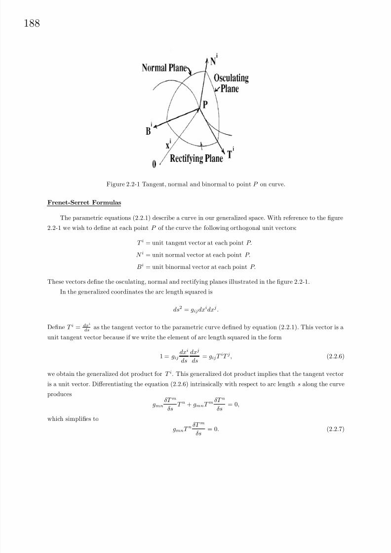
8/6/2019 Introduction to Tensor Calculus Continuum Mechanics - J. Heinbockel
http://slidepdf.com/reader/full/introduction-to-tensor-calculus-continuum-mechanics-j-heinbockel 193/372
188
Figure 2.2-1 Tangent, normal and binormal to point P on curve.
Frenet-Serret Formulas
The parametric equations (2.2.1) describe a curve in our generalized space. With reference to the figure
2.2-1 we wish to define at each point P of the curve the following orthogonal unit vectors:
T i = unit tangent vector at each point P.
N i = unit normal vector at each point P.
Bi = unit binormal vector at each point P.
These vectors define the osculating, normal and rectifying planes illustrated in the figure 2.2-1.
In the generalized coordinates the arc length squared is
ds2 = gijdxidxj .
Define T i = dxi
ds as the tangent vector to the parametric curve defined by equation (2.2.1). This vector is a
unit tangent vector because if we write the element of arc length squared in the form
1 = gijdxi
ds
dxj
ds= gijT iT j, (2.2.6)
we obtain the generalized dot product for T i. This generalized dot product implies that the tangent vector
is a unit vector. Differentiating the equation (2.2.6) intrinsically with respect to arc length s along the curve
produces
gmnδT m
δsT n + gmnT m
δT n
δs= 0,
which simplifies to
gmnT nδT m
δs= 0. (2.2.7)
8/6/2019 Introduction to Tensor Calculus Continuum Mechanics - J. Heinbockel
http://slidepdf.com/reader/full/introduction-to-tensor-calculus-continuum-mechanics-j-heinbockel 194/372
18
The equation (2.2.7) is a statement that the vector δT m
δs is orthogonal to the vector T m. The unit normal
vector is defined as
N i =1
κ
δT i
δsor N i =
1
κ
δT iδs
, (2.2.8)
where κ is a scalar called the curvature and is chosen such that the magnitude of N i is unity. The reciprocal
of the curvature is R =1
κ , which is called the radius of curvature. The curvature of a straight line is zerowhile the curvature of a circle is a constant. The curvature measures the rate of change of the tangent vector
as the arc length varies.
The equation (2.2.7) can be expressed in the form
gijT iN j = 0. (2.2.9)
Taking the intrinsic derivative of equation (2.2.9) with respect to the arc length s produces
gijT iδN j
δs+ gij
δT i
δsN j = 0
orgijT i
δN j
δs= −gij
δT i
δsN j = −κgijN iN j = −κ. (2.2.10)
The generalized dot product can be written
gijT iT j = 1,
and consequently we can express equation (2.2.10) in the form
gijT iδN j
δs= −κgijT iT j or gijT i
δN j
δs+ κT j
= 0. (2.2.11)
Consequently, the vector δN j
δs+ κT j (2.2.12)
is orthogonal to T i. In a similar manner, we can use the relation gijN iN j = 1 and differentiate intrinsically
with respect to the arc length s to show that
gijN iδN j
δs= 0.
This in turn can be expressed in the form
gijN i
δN j
δs+ κT j
= 0.
This form of the equation implies that the vector represented in equation (2.2.12) is also orthogonal to the
unit normal N i. We define the unit binormal vector as
Bi =1
τ
δN i
δs+ κT i
or Bi =
1
τ
δN iδs
+ κT i
(2.2.13)
where τ is a scalar called the torsion. The torsion is chosen such that the binormal vector is a unit vector.
The torsion measures the rate of change of the osculating plane and consequently, the torsion τ is a measure
8/6/2019 Introduction to Tensor Calculus Continuum Mechanics - J. Heinbockel
http://slidepdf.com/reader/full/introduction-to-tensor-calculus-continuum-mechanics-j-heinbockel 195/372
190
of the twisting of the curve out of a plane. The value τ = 0 corresponds to a plane curve. The vectors
T i, N i, Bi, i = 1, 2, 3 satisfy the cross product relation
Bi = ijkT jN k.
If we differentiate this relation intrinsically with respect to arc length s we find
δBi
δs= ijk
T j
δN kδs
+δT jδs
N k
= ijk [T j(τBk − κT k) + κN jN k]
= τ ijkT jBk = −τ ikjBkT j = −τ N i.
(2.2.14)
The relations (2.2.8),(2.2.13) and (2.2.14) are now summarized and written
δT i
δs= κN i
δN i
δs = τBi
− κT i
δBi
δs= −τ N i.
(2.2.15)
These equations are known as the Frenet-Serret formulas of differential geometry.
Velocity and Acceleration
Chain rule differentiation of the generalized velocity is expressible in the form
vi =dxi
dt=
dxi
ds
ds
dt= T iv, (2.2.16)
where v = dsdt is the speed of the particle and is the magnitude of vi. The vector T i is the unit tangent vector
to the trajectory curve at the time t. The equation (2.2.16) is a statement of the fact that the velocity of a
particle is always in the direction of the tangent vector to the curve and has the speed v.
By chain rule differentiation, the generalized acceleration is expressible in the form
f r =δvr
δt=
dv
dtT r + v
δT r
δt
=dv
dtT r + v
δT r
δs
ds
dt
=dv
dtT r + κv2N r.
(2.2.17)
The equation (2.2.17) states that the acceleration lies in the osculating plane. Further, the equation (2.2.17)
indicates that the tangential component of the acceleration is dvdt , while the normal component of the accel-
eration is κv2.

8/6/2019 Introduction to Tensor Calculus Continuum Mechanics - J. Heinbockel
http://slidepdf.com/reader/full/introduction-to-tensor-calculus-continuum-mechanics-j-heinbockel 196/372
19
Work and Potential Energy
Define M as the constant mass of the particle as it moves along the curve defined by equation (2.2.1).
Also let Qr denote the components of a force vector (in appropriate units of measurements) which acts upon
the particle. Newton’s second law of motion can then be expressed in the form
Qr = M f r or Qr = M f r. (2.2.18)
The work done W in moving a particle from a point P 0 to a point P 1 along a curve xr = xr(t), r = 1, 2, 3,
with parameter t, is represented by a summation of the tangential components of the forces acting along the
path and is defined as the line integral
W =
P 1
P 0
Qrdxr
dsds =
P 1
P 0
Qr dxr =
t1t0
Qrdxr
dtdt =
t1t0
Qrvr dt (2.2.19)
where Qr = grsQs is the covariant form of the force vector, t is the time parameter and s is arc length along
the curve.
Conservative Systems
If the force vector is conservative it means that the force is derivable from a scalar potential function
V = V (x1, x2, . . . , xN ) such that Qr = −V ,r = − ∂V
∂xr, r = 1, . . . , N . (2.2.20)
In this case the equation (2.2.19) can be integrated and we find that to within an additive constant we will
have V = −W. The potential function V is called the potential energy of the particle and the work done
becomes the change in potential energy between the starting and end points and is independent of the path
connecting the points.
Lagrange’s Equations of Motion
The kinetic energy T of the particle is defined as one half the mass times the velocity squared and can
be expressed in any of the forms
T =1
2M
ds
dt
2
=1
2M v2 =
1
2M gmnvmvn =
1
2M gmnxmxn, (2.2.21)
where the dot notation denotes differentiation with respect to time. It is an easy exercise to calculate the
derivatives∂T
∂ xr
= M grmxm
d
dt
∂T
∂ xr
= M
grmxm +
∂grm
∂xnxnxm
∂T
∂xr=
1
2M
∂gmn
∂xrxmxn,
(2.2.22)
and thereby verify the relation
d
dt
∂T
∂ xr
− ∂T
∂xr= M f r = Qr, r = 1, . . . , N . (2.2.23)

8/6/2019 Introduction to Tensor Calculus Continuum Mechanics - J. Heinbockel
http://slidepdf.com/reader/full/introduction-to-tensor-calculus-continuum-mechanics-j-heinbockel 197/372
192
This equation is called the Lagrange’s form of the equations of motion.
EXAMPLE 2.2-1. (Equations of motion in spherical coordinates) Find the Lagrange’s form of
the equations of motion in spherical coordinates.
Solution: Let x1 = ρ, x2 = θ, x3 = φ then the element of arc length squared in spherical coordinates has
the formds2 = (dρ)2 + ρ2(dθ)2 + ρ2 sin2 θ(dφ)2.
The element of arc length squared can be used to construct the kinetic energy. For example,
T =1
2M
ds
dt
2
=1
2M
( ρ)2 + ρ2(θ)2 + ρ2 sin2 θ(φ)2
.
The Lagrange form of the equations of motion of a particle are found from the relations (2.2.23) and are
calculated to be:
Mf 1 = Q1 =d
dt ∂T
∂ ρ− ∂T
∂ρ= M
ρ − ρ(θ)2 − ρ sin2 θ(φ)2
Mf 2 = Q2 =
ddt∂T
∂ θ
− ∂T ∂θ
= M d
dt
ρ2θ− ρ2 sin θ cos θ(φ)2
Mf 3 = Q3 =
d
dt
∂T
∂ φ
− ∂T
∂φ= M
d
dt
ρ2 sin2 θφ
.
In terms of physical components we have
Qρ = M
ρ − ρ(θ)2 − ρ sin2 θ(φ)2
Qθ =M
ρ
d
dt
ρ2θ
− ρ2 sin θ cos θ(φ)2
Qφ =
M
ρ sin θ d
dt ρ2 sin2 θφ .
Euler-Lagrange Equations of Motion
Starting with the Lagrange’s form of the equations of motion from equation (2.2.23), we assume that
the external force Qr is derivable from a potential function V as specified by the equation (2.2.20). That is,
we assume the system is conservative and express the equations of motion in the form
d
dt
∂T
∂ xr
− ∂T
∂xr= − ∂V
∂xr= Qr, r = 1, . . . , N (2.2.24)
The Lagrangian is defined by the equation
L = T − V = T (x1, . . . , xN , x1, . . . , xN ) − V (x1, . . . , xN ) = L(xi, xi). (2.2.25)
Employing the defining equation (2.2.25), it is readily verified that the equations of motion are expressible
in the formd
dt
∂L
∂ xr
− ∂L
∂xr= 0, r = 1, . . . , N , (2.2.26)
which are called the Euler-Lagrange form for the equations of motion.

8/6/2019 Introduction to Tensor Calculus Continuum Mechanics - J. Heinbockel
http://slidepdf.com/reader/full/introduction-to-tensor-calculus-continuum-mechanics-j-heinbockel 198/372

8/6/2019 Introduction to Tensor Calculus Continuum Mechanics - J. Heinbockel
http://slidepdf.com/reader/full/introduction-to-tensor-calculus-continuum-mechanics-j-heinbockel 199/372
194
EXAMPLE 2.2-3. (Simple pendulum) Find the equation of motion for the pendulum system illus-
trated in the figure 2.2-3.
Solution: Choose the angle θ illustrated in the figure 2.2-3 as the generalized coordinate. If the pendulum
is moved from a vertical position through an angle θ, we observe that the mass m moves up a distance
h =
− cos θ. The work done in moving this mass a vertical distance h is
W = −mgh = −mg(1− cos θ),
since the force is −mg in this coordinate system. In moving the pendulum through an angle θ, the arc length
s swept out by the mass m is s = θ. This implies that the kinetic energy can be expressed
T =1
2m
ds
dt
2
=1
2m
θ2
=1
2m2(θ)2.
Figure 2.2-3 Simple pendulum system
The Lagrangian of the system is
L = T − V =1
2m2(θ)2 − mg(1− cos θ)
and from this we find the equation of motion
d
dt ∂L
∂ θ −∂L
∂θ = 0 ord
dt m2θ− mg(− sin θ) = 0.
This in turn simplifies to the equation
θ +g
sin θ = 0.
This equation together with a set of initial conditions for θ and θ represents the nonlinear differential equation
which describes the motion of a pendulum without damping.

8/6/2019 Introduction to Tensor Calculus Continuum Mechanics - J. Heinbockel
http://slidepdf.com/reader/full/introduction-to-tensor-calculus-continuum-mechanics-j-heinbockel 200/372
19
EXAMPLE 2.2-4. (Compound pendulum) Find the equations of motion for the compound pendulum
illustrated in the figure 2.2-4.
Solution: Choose for the generalized coordinates the angles x1 = θ1 and x2 = θ2 illustrated in the figure
2.2-4. To find the potential function V for this system we consider the work done as the masses m1 and
m2 are moved. Consider independent motions of the angles θ1 and θ2. Imagine the compound pendulum
initially in the vertical position as illustrated in the figure 2.2-4(a). Now let m1 be displaced due to a change
in θ1 and obtain the figure 2.2-4(b). The work done to achieve this position is
W 1 = −(m1 + m2)gh1 = −(m1 + m2)gL1(1 − cos θ1).
Starting from the position in figure 2.2-4(b) we now let θ2 undergo a displacement and achieve the configu-
ration in the figure 2.2-4(c).
Figure 2.2-4 Compound pendulum
The work done due to the displacement θ2 can be represented
W 2 = −m2gh2 = −m2gL2(1 − cos θ2).
Since the potential energy V satisfies V = −W to within an additive constant, we can write
V = −W = −W 1 − W 2 = −(m1 + m2)gL1 cos θ1 − m2gL2 cos θ2 + constant,
where the constant term in the potential energy has been neglected since it does not contribute anything to
the equations of motion. (i.e. the derivative of a constant is zero.)
The kinetic energy term for this system can be represented
T =1
2m1
ds1dt
2
+1
2m2
ds2dt
2
T =1
2m1(x21 + y21) +
1
2m2(x22 + y22),
(2.2.27)

8/6/2019 Introduction to Tensor Calculus Continuum Mechanics - J. Heinbockel
http://slidepdf.com/reader/full/introduction-to-tensor-calculus-continuum-mechanics-j-heinbockel 201/372
196
where(x1, y1) = (L1 sin θ1 , −L1 cos θ1)
(x2, y2) = (L1 sin θ1 + L2 sin θ2,−L1 cos θ1 − L2 cos θ2)(2.2.28)
are the coordinates of the masses m1 and m2 respectively. Substituting the equations (2.2.28) into equation
(2.2.27) and simplifying produces the kinetic energy expression
T =1
2(m1 + m2)L2
1θ21 + m2L1L2θ1θ2 cos(θ1 − θ2) +1
2m2L2
2θ22 . (2.2.29)
Writing the Lagrangian as L = T −V , the equations describing the motion of the compound pendulum
are obtained from the Lagrangian equations
d
dt
∂L
∂ θ1
− ∂L
∂θ1= 0 and
d
dt
∂L
∂ θ2
− ∂L
∂θ2= 0.
Calculating the necessary derivatives, substituting them into the Lagrangian equations of motion and then
simplifying we derive the equations of motion
L1θ1 + m2
m1 + m2L2θ2 cos(θ1 − θ2) + m2
m1 + m2L2(θ2)2 sin(θ1 − θ2) + g sin θ1 = 0
L1θ1 cos(θ1 − θ2) + L2θ2 − L1(θ1)2 sin(θ1 − θ2) + g sin θ2 = 0.
These equations are a set of coupled, second order nonlinear ordinary differential equations. These equations
are subject to initial conditions being imposed upon the angular displacements (θ1, θ2) and the angular
velocities (θ1, θ2).
Alternative Derivation of Lagrange’s Equations of Motion
Let c denote a given curve represented in the parametric form
xi = xi(t), i = 1, . . . , N, t0 ≤ t ≤ t1
and let P 0, P 1 denote two points on this curve corresponding to the parameter values t0 and t1 respectively.
Let c denote another curve which also passes through the two points P 0 and P 1 as illustrated in the figure
2.2-5.
The curve c is represented in the parametric form
xi = xi(t) = xi(t) + ηi(t), i = 1, . . . , N, t0 ≤ t ≤ t1
in terms of a parameter . In this representation the function ηi(t) must satisfy the end conditions
ηi(t0) = 0 and ηi(t1) = 0 i = 1, . . . , N
since the curve c is assumed to pass through the end points P 0 and P 1.
Consider the line integral
I () =
t1t0
L(t, xi + ηi, xi + ηi) dt, (2.2.30)
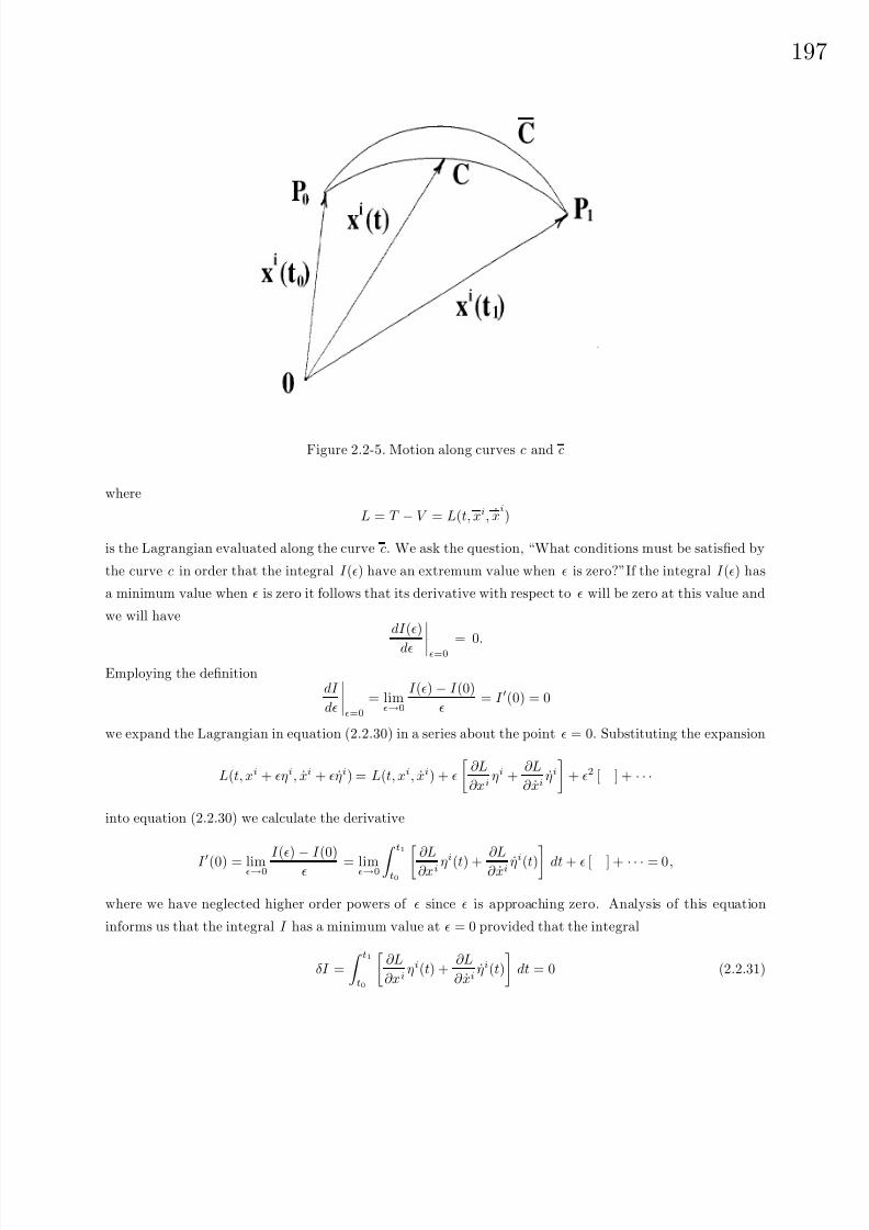
8/6/2019 Introduction to Tensor Calculus Continuum Mechanics - J. Heinbockel
http://slidepdf.com/reader/full/introduction-to-tensor-calculus-continuum-mechanics-j-heinbockel 202/372
19
Figure 2.2-5. Motion along curves c and c
where
L = T − V = L(t, xi, xi)
is the Lagrangian evaluated along the curve c. We ask the question, “What conditions must be satisfied by
the curve c in order that the integral I () have an extremum value when is zero?”If the integral I () has
a minimum value when is zero it follows that its derivative with respect to will be zero at this value and
we will havedI ()
d =0
= 0.
Employing the definitiondI
d
=0
= lim→0
I () − I (0)
= I (0) = 0
we expand the Lagrangian in equation (2.2.30) in a series about the point = 0. Substituting the expansion
L(t, xi + ηi, xi + ηi) = L(t, xi, xi) +
∂L
∂xiηi +
∂L
∂ xiηi
+ 2 [ ] + · · ·
into equation (2.2.30) we calculate the derivative
I (0) = lim→0
I ()−
I (0)
= lim→0 t1t0 ∂L
∂xi ηi(t) +∂L
∂ xi ηi(t) dt + [ ] + · · · = 0,
where we have neglected higher order powers of since is approaching zero. Analysis of this equation
informs us that the integral I has a minimum value at = 0 provided that the integral
δI =
t1t0
∂L
∂xiηi(t) +
∂L
∂ xiηi(t)
dt = 0 (2.2.31)
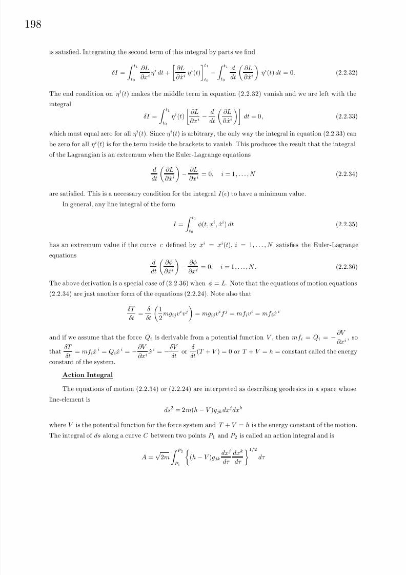
8/6/2019 Introduction to Tensor Calculus Continuum Mechanics - J. Heinbockel
http://slidepdf.com/reader/full/introduction-to-tensor-calculus-continuum-mechanics-j-heinbockel 203/372
198
is satisfied. Integrating the second term of this integral by parts we find
δI =
t1t0
∂L
∂xiηi dt +
∂L
∂ xiηi(t)
t1t0
− t1t0
d
dt
∂L
∂ xi
ηi(t) dt = 0. (2.2.32)
The end condition on ηi(t) makes the middle term in equation (2.2.32) vanish and we are left with the
integral
δI =
t1t0
ηi(t)
∂L
∂xi− d
dt
∂L
∂ xi
dt = 0, (2.2.33)
which must equal zero for all ηi(t). Since ηi(t) is arbitrary, the only way the integral in equation (2.2.33) can
be zero for all ηi(t) is for the term inside the brackets to vanish. This produces the result that the integral
of the Lagrangian is an extremum when the Euler-Lagrange equations
d
dt
∂L
∂ xi
− ∂L
∂xi= 0, i = 1, . . . , N (2.2.34)
are satisfied. This is a necessary condition for the integral I () to have a minimum value.
In general, any line integral of the form
I =
t1t0
φ(t, xi, xi) dt (2.2.35)
has an extremum value if the curve c defined by xi = xi(t), i = 1, . . . , N satisfies the Euler-Lagrange
equationsd
dt
∂φ
∂ xi
− ∂φ
∂xi= 0, i = 1, . . . , N . (2.2.36)
The above derivation is a special case of (2.2.36) when φ = L. Note that the equations of motion equations
(2.2.34) are just another form of the equations (2.2.24). Note also that
δT
δt=
δ
δt
1
2mgijvivj
= mgijvif j = mf iv
i = mf ixi
and if we assume that the force Qi is derivable from a potential function V , then mf i = Qi = −∂V
∂xi, so
thatδT
δt= mf ix
i = Qixi = − ∂V
∂xix i = −δV
δtor
δ
δt(T + V ) = 0 or T + V = h = constant called the energy
constant of the system.
Action Integral
The equations of motion (2.2.34) or (2.2.24) are interpreted as describing geodesics in a space whose
line-element isds2 = 2m(h − V )gjkdxjdxk
where V is the potential function for the force system and T + V = h is the energy constant of the motion.
The integral of ds along a curve C between two points P 1 and P 2 is called an action integral and is
A =√
2m
P 2
P 1
(h − V )gjk
dxj
dτ
dxk
dτ
1/2
dτ

8/6/2019 Introduction to Tensor Calculus Continuum Mechanics - J. Heinbockel
http://slidepdf.com/reader/full/introduction-to-tensor-calculus-continuum-mechanics-j-heinbockel 204/372

8/6/2019 Introduction to Tensor Calculus Continuum Mechanics - J. Heinbockel
http://slidepdf.com/reader/full/introduction-to-tensor-calculus-continuum-mechanics-j-heinbockel 205/372
200
Employing the e − δ identity the equation (2.2.38) can be simplified to the form
T =1
2
N α=1
m(α)
ωmωmx
(α)k x
(α)k − ωnωkx
(α)k x(α)
n
.
Define the second moments and products of inertia by the equation
I ij =N
α=1
m(α)
x(α)k x
(α)k δij − x
(α)i x
(α)j
(2.2.39)
and write the kinetic energy in the form
T =1
2I ijωiωj . (2.2.40)
Similarly, the angular momentum of the system of particles can also be represented in terms of the
second moments and products of inertia. The angular momentum of a system of particles is defined as a
summation of the moments of the linear momentum of each individual particle and is
H i =N
α=1
m(α)eijkx(α)j v
(α)k =
N α=1
m(α)eijkx(α)j ekmnωmx(α)
n . (2.2.41)
The e − δ identity simplifies the equation (2.2.41) to the form
H i = ωj
N α=1
m(α)
x(α)n x(α)
n δij − x(α)j x
(α)i
= ωjI ji. (2.2.42)
The equations of motion of a rigid body is obtained by applying Newton’s second law of motion to the
system of N particles. The equation of motion of the αth particle is written
m(α)x(α)i = F
(α)i . (2.2.43)
Summing equation (2.2.43) over all particles gives the result
N α=1
m(α)x(α)i =
N α=1
F (α)i . (2.2.44)
This represents the translational equations of motion of the rigid body. The equation (2.2.44) represents the
rate of change of linear momentum being equal to the total external force acting upon the system. Taking
the cross product of equation (2.2.43) with the position vector x(α)j produces
m(α)x(α)t erstx(α)s = erstx(α)s F (α)t
and summing over all particles we find the equation
N α=1
m(α)erstx(α)s x
(α)t =
N α=1
erstx(α)s F (α)t . (2.2.45)

8/6/2019 Introduction to Tensor Calculus Continuum Mechanics - J. Heinbockel
http://slidepdf.com/reader/full/introduction-to-tensor-calculus-continuum-mechanics-j-heinbockel 206/372
20
The equations (2.2.44) and (2.2.45) represent the conservation of linear and angular momentum and can be
written in the formsd
dt
N
α=1
m(α)x(α)r
=
N α=1
F (α)r (2.2.46)
and
ddt N
α=1
m(α)erstx(α)s x
(α)t =
N α=1
erstx(α)s F
(α)t . (2.2.47)
By definition we have Gr =
m(α)x(α)r representing the linear momentum, F r =
F (α)r the total force
acting on the system of particles, H r =
m(α)erstx(α)s x
(α)t is the angular momentum of the system relative
to the origin, and M r =
erstx(α)s F
(α)t is the total moment of the system relative to the origin. We can
therefore express the equations (2.2.46) and (2.2.47) in the form
dGr
dt= F r (2.2.48)
and
dH rdt
= M r. (2.2.49)
The equation (2.2.49) expresses the fact that the rate of change of angular momentum is equal to the
moment of the external forces about the origin. These equations show that the motion of a system of
particles can be studied by considering the motion of the center of mass of the system (translational motion)
and simultaneously considering the motion of points about the center of mass (rotational motion).
We now develop some relations in order to express the equations (2.2.49) in an alternate form. Toward
this purpose we consider first the concepts of relative motion and angular velocity.
Relative Motion and Angular Velocity
Consider two different reference frames denoted by S and S . Both reference frames are Cartesiancoordinates with axes xi and xi , i = 1, 2, 3, respectively. The reference frame S is fixed in space and is
called an inertial reference frame or space-fixed reference system of axes. The reference frame S is fixed
to and rotates with the rigid body and is called a body-fixed system of axes. Again, for convenience, it
is assumed that the origins of both reference systems are fixed at the center of mass of the rigid body.
Further, we let the system S have the basis vectors ei, i = 1, 2, 3, while the reference system S has the basis
vectors ei , i = 1, 2, 3. The transformation equations between the two sets of reference axes are the affine
transformations
xi = jixj and xi = ijxj (2.2.50)
where ij = ij(t) are direction cosines which are functions of time t (i.e. the ij are the cosines of theangles between the barred and unbarred axes where the barred axes are rotating relative to the space-fixed
unbarred axes.) The direction cosines satisfy the relations
ijik = δjk and ijkj = δik. (2.2.51)
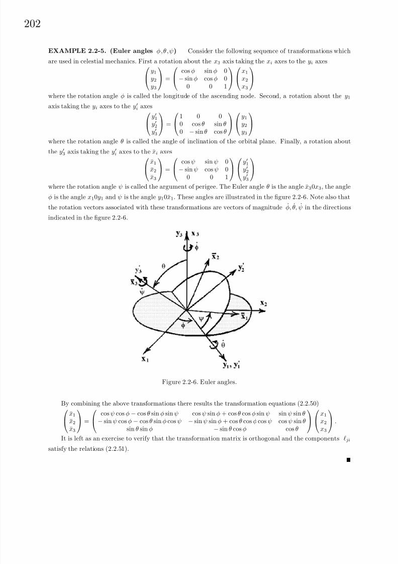
8/6/2019 Introduction to Tensor Calculus Continuum Mechanics - J. Heinbockel
http://slidepdf.com/reader/full/introduction-to-tensor-calculus-continuum-mechanics-j-heinbockel 207/372
202
EXAMPLE 2.2-5. (Euler angles φ,θ,ψ) Consider the following sequence of transformations which
are used in celestial mechanics. First a rotation about the x3 axis taking the xi axes to the yi axes y1y2y3
=
cos φ sin φ 0− sin φ cos φ 0
0 0 1
x1
x2
x3
where the rotation angle φ is called the longitude of the ascending node. Second, a rotation about the y1axis taking the yi axes to the yi axes y1
y2y3
=
1 0 00 cos θ sin θ0 − sin θ cos θ
y1y2y3
where the rotation angle θ is called the angle of inclination of the orbital plane. Finally, a rotation about
the y3 axis taking the yi axes to the xi axes x1
x2
x3
=
cos ψ sin ψ 0− sin ψ cos ψ 0
0 0 1
y1y2y3
where the rotation angle ψ is called the argument of perigee. The Euler angle θ is the angle x30x3, the angle
φ is the angle x10y1 and ψ is the angle y10x1. These angles are illustrated in the figure 2.2-6. Note also thatthe rotation vectors associated with these transformations are vectors of magnitude φ, θ, ψ in the directions
indicated in the figure 2.2-6.
Figure 2.2-6. Euler angles.
By combining the above transformations there results the transformation equations (2.2.50) x1x2x3
=
cos ψ cos φ − cos θ sin φ sin ψ cos ψ sin φ + cos θ cos φ sin ψ sin ψ sin θ− sin ψ cos φ − cos θ sin φ cos ψ − sin ψ sin φ + cos θ cos φ cos ψ cos ψ sin θ
sin θ sin φ − sin θ cos φ cos θ
x1
x2
x3
.
It is left as an exercise to verify that the transformation matrix is orthogonal and the components ji
satisfy the relations (2.2.51).

8/6/2019 Introduction to Tensor Calculus Continuum Mechanics - J. Heinbockel
http://slidepdf.com/reader/full/introduction-to-tensor-calculus-continuum-mechanics-j-heinbockel 208/372
20
Consider the velocity of a point which is rotating with the rigid body. Denote by vi = vi(S ), for
i = 1, 2, 3, the velocity components relative to the S reference frame and by vi = vi(S ), i = 1, 2, 3 the
velocity components of the same point relative to the body-fixed axes. In terms of the basis vectors we can
write
V = v1(S ) e1 + v2(S ) e2 + v3(S ) e3 =dxi
dt
ei (2.2.52)
as the velocity in the S reference frame. Similarly, we write
V = v1(S ) e1 + v2(S ) e2 + v3(S ) e3 =dxi
dt ei (2.2.53)
as the velocity components relative to the body-fixed reference frame. There are occasions when it is desirable
to represent V in the S frame of reference and V in the S frame of reference. In these instances we can write
V = v1(S ) e1 + v2(S ) e2 + v3(S ) e3 (2.2.54)
and V = v1(S ) e1 + v2(S ) e2 + v3(S ) e3. (2.2.55)
Here we have adopted the notation that vi(S ) are the velocity components relative to the S reference frame
and vi(S ) are the same velocity components relative to the S reference frame. Similarly, vi(S ) denotes the
velocity components relative to the S reference frame, while vi(S ) denotes the same velocity components
relative to the S reference frame.
Here both V and V are vectors and so their components are first order tensors and satisfy the transfor-
mation laws
vi(S ) = jivj(S ) = jixj and vi(S ) = ijvj(S ) = ij xj. (2.2.56)
The equations (2.2.56) define the relative velocity components as functions of time t. By differentiating the
equations (2.2.50) we obtaindxi
dt= vi(S ) = jixj + jixj (2.2.57)
anddxi
dt= vi(S ) = ij xj + ijxj . (2.2.58)
Multiply the equation (2.2.57) by mi and multiply the equation (2.2.58) by im and derive the relations
vm(S ) = vm(S ) + mijixj (2.2.59)
and
vm(S ) = vm(S ) + im˙ijxj . (2.2.60)
The equations (2.2.59) and (2.2.60) describe the transformation laws of the velocity components upon chang-
ing from the S to the S reference frame. These equations can be expressed in terms of the angular velocity
by making certain substitutions which are now defined.
The first order angular velocity vector ωi is related to the second order skew-symmetric angular velocity
tensor ωij by the defining equation
ωmn = eimnωi. (2.2.61)

8/6/2019 Introduction to Tensor Calculus Continuum Mechanics - J. Heinbockel
http://slidepdf.com/reader/full/introduction-to-tensor-calculus-continuum-mechanics-j-heinbockel 209/372
8/6/2019 Introduction to Tensor Calculus Continuum Mechanics - J. Heinbockel
http://slidepdf.com/reader/full/introduction-to-tensor-calculus-continuum-mechanics-j-heinbockel 210/372
20
Now if we multiply equation (2.2.49) by erjk , then it can be written in the form
dH ijdt
= M ij. (2.2.67)
Similarly, if we multiply the equation (2.2.42) by eimn, then it can be expressed in the alternate form
H mn = eimnωjI ji = I mnstωst
and because of this relation the equation (2.2.67) can be expressed as
d
dt(I ijstωst) = M ij. (2.2.68)
We write this equation in the barred system of coordinates where I pqrs will be a constant and consequently
its derivative will be zero. We employ the transformation equations
I ijst = ipjqsrtkI pqrk
ωij = sitjωst
M pq = ipjqM ij
and then multiply the equation (2.2.68) by ipjq and simplify to obtain
ipjqd
dt
iαjβI αβrkωrk
= M pq.
Expand all terms in this equation and take note that the derivative of the I αβrk is zero. The expanded
equation then simplifies to
I pqrkdωrk
dt+ (δαuδ pvδβq + δ pαδβuδqv) I αβrkωrkωuv = M pq. (2.2.69)
Substitute into equation (2.2.69) the relations from equations (2.2.61),(2.2.64) and (2.2.66), and then multiply
by empq and simplify to obtain the Euler’s equations of motion
I imdωi
dt− etmjI ijωiωt = M m. (2.2.70)
Dropping the bar notation and performing the indicated summations over the range 1,2,3 we find the
Euler equations have the form
I 11dω1
dt+ I 21
dω2
dt+ I 31
dω3
dt+ (I 13ω1 + I 23ω2 + I 33ω3) ω2 − (I 12ω1 + I 22ω2 + I 32ω3) ω3 = M 1
I 12dω1
dt+ I 22
dω2
dt+ I 32
dω3
dt+ (I 11ω1 + I 21ω2 + I 31ω3) ω3 − (I 13ω1 + I 23ω2 + I 33ω3) ω1 = M 2
I 13dω1
dt+ I 23
dω2
dt+ I 33
dω3
dt+ (I 12ω1 + I 22ω2 + I 32ω3) ω1 − (I 11ω1 + I 21ω2 + I 31ω3) ω2 = M 3.
(2.2.71)
In the special case where the barred axes are principal axes, then I ij = 0 for i = j and the Euler’s
equations reduces to the system of nonlinear differential equations
I 11dω1
dt+ (I 33 − I 22)ω2ω3 = M 1
I 22dω2
dt+ (I 11 − I 33)ω3ω1 = M 2
I 33dω3
dt+ (I 22 − I 11)ω1ω2 = M 3.
(2.2.72)
In the case of constant coefficients and constant moments the solutions of the above differential equations
can be expressed in terms of Jacobi elliptic functions.

8/6/2019 Introduction to Tensor Calculus Continuum Mechanics - J. Heinbockel
http://slidepdf.com/reader/full/introduction-to-tensor-calculus-continuum-mechanics-j-heinbockel 211/372

8/6/2019 Introduction to Tensor Calculus Continuum Mechanics - J. Heinbockel
http://slidepdf.com/reader/full/introduction-to-tensor-calculus-continuum-mechanics-j-heinbockel 212/372
20
Figure 2.2-7. Pulley and mass system
17. For the pulley and mass system illustrated in the figure 2.2-7 let
a = the radius of each pulley.
1 = the length of the upper chord.
2 = the length of the lower chord.
Neglect the weight of the pulley and find the equations of motion for the pulley mass system.
18. Let φ = dsdt
, where s is the arc length between two points on a curve in generalized coordinates.
(a) Write the arc length in general coordinates as ds =
gmnxmxndt and show the integral I , defined by
equation (2.2.35), represents the distance between two points on a curve.
(b) Using the Euler-Lagrange equations (2.2.36) show that the shortest distance between two points in a
generalized space is the curve defined by the equations: xi +
i
j k
xj xk = xi
d2sdt2
dsdt
(c) Show in the special case t = s the equations in part (b) reduce tod2xi
ds2+
i
j k
dxj
ds
dxk
ds= 0, for
i = 1, . . . , N . An examination of equation (1.5.51) shows that the above curves are geodesic curves.
(d) Show that the shortest distance between two points in a plane is a straight line.
(e) Consider two points on the surface of a cylinder of radius a. Let u1 = θ and u2 = z denote surface
coordinates in the two dimensional space defined by the surface of the cylinder. Show that the shortest
distance between the points where θ = 0, z = 0 and θ = π, z = H is L = a2π2 + H 2.
19. For T = 12
mgijvivj the kinetic energy of a particle and V the potential energy of the particle show
that T + V = constant.
Hint: mf i = Qi = − ∂V ∂xi , i = 1, 2, 3 and dxi
dt = xi = vi, i = 1, 2, 3.

8/6/2019 Introduction to Tensor Calculus Continuum Mechanics - J. Heinbockel
http://slidepdf.com/reader/full/introduction-to-tensor-calculus-continuum-mechanics-j-heinbockel 213/372
208
20. Define H = T + V as the sum of the kinetic energy and potential energy of a particle. The quantity
H = H (xr, pr) is called the Hamiltonian of the particle and it is expressed in terms of:
• the particle position xi and
• the particle momentum pi = mvi = mgijxj . Here xrand pr are treated as independent variables.
(a) Show that the particle momentum is a covariant tensor of rank 1.(b) Express the kinetic energy T in terms of the particle momentum.
(c) Show that pi =∂T
∂ xi.
(d) Show thatdxi
dt=
∂H
∂piand
dpi
dt= −∂H
∂xi. These are a set of differential equations describing the
position change and momentum change of the particle and are known as Hamilton’s equations of motion
for a particle.
21. Let δT i
δs = κN i and δN i
δs = τ Bi − κT i and calculate the intrinsic derivative of the cross product
Bi = ijkT jN k and find δBi
δs in terms of the unit normal vector.
22. For T the kinetic energy of a particle and V the potential energy of a particle, define the Lagrangian
L = L(xi, xi) = T − V =1
2Mgijxixj − V as a function of the independent variables xi, xi. Define the
Hamiltonian H = H (xi, pi) = T + V =1
2M gij pi pj + V, as a function of the independent variables xi, pi,
where pi is the momentum vector of the particle and M is the mass of the particle.
(a) Show that pi =∂T
∂ xi.
(b) Show that∂H
∂xi= − ∂L
∂xi
23. When the Euler angles, figure 2.2-6, are applied to the motion of rotating objects, θ is the angle
of nutation, φ is the angle of precession and ψ is the angle of spin. Take projections and show that the
time derivative of the Euler angles are related to the angular velocity vector components ωx, ωy, ωz by the
relationsωx = θ cos ψ + φ sin θ sin ψ
ωy = −θ sin ψ + φ sin θ cos ψ
ωz = ψ + φ cos θ
where ωx, ωy, ωz are the angular velocity components along the x1, x2, x3 axes.
24. Find the equations of motion for the compound pendulum illustrated in the figure 2.2-8.
25. Let F = −GMmr3
r denote the inverse square law force of attraction between the earth and sun, with
G a universal constant, M the mass of the sun, m the mass of the earth and rr a unit vector from origin
at the center of the sun pointing toward the earth. (a) Write down Newton’s second law, in both vector
and tensor form, which describes the motion of the earth about the sun. (b) Show thatd
dt(r × v) = 0 and
consequently r × v = r × drdt = h = a constant.

8/6/2019 Introduction to Tensor Calculus Continuum Mechanics - J. Heinbockel
http://slidepdf.com/reader/full/introduction-to-tensor-calculus-continuum-mechanics-j-heinbockel 214/372
20
Figure 2.2-8. Compound pendulum
26. Construct a set of axes fixed and attached to an airplane. Let the x axis be a longitudinal axis running
from the rear to the front of the plane along its center line. Let the y axis run between the wing tips and
let the z axis form a right-handed system of coordinates. The y axis is called a lateral axis and the z axis is
called a normal axis. Define pitch as any angular motion about the lateral axis. Define roll as any angular
motion about the longitudinal axis. Define yaw as any angular motion about the normal axis. Consider two
sets of axes. One set is the x, y, z axes attached to and moving with the aircraft. The other set of axes is
denoted X, Y, Z and is fixed in space ( an inertial set of axes). Describe the pitch, roll and yaw of an aircraft
with respect to the inertial set of axes. Show the transformation is orthogonal. Hint: Consider pitch with
respect to the fixed axes, then consider roll with respect to the pitch axes and finally consider yaw with
respect to the roll axes. This produces three separate transformation matrices which can then be combined
to describe the motions of pitch, roll and yaw of an aircraft.
27. In Cartesian coordinates let F i = F i(x1, x2, x3) denote a force field and let xi = xi(t) denote a curve
C . (a) Show Newton’s second law implies that along the curve C d
dt
1
2m
dxi
dt
2
= F i(x1, x2, x3)dxi
dt
(no summation on i) and hence
d
dt
1
2m
dx1
dt 2
+
dx2
dt 2
+
dx3
dt 2
=d
dt 1
2mv2
= F 1
dx1
dt+ F 2
dx2
dt+ F 3
dx3
dt
(b) Consider two points on the curve C , say point A, xi(tA) and point B, xi(tB) and show that the work
done in moving from A to B in the force field F i is
1
2mv2
tBtA
=
BA
F idx1 + F 2dx2 + F 3dx3
8/6/2019 Introduction to Tensor Calculus Continuum Mechanics - J. Heinbockel
http://slidepdf.com/reader/full/introduction-to-tensor-calculus-continuum-mechanics-j-heinbockel 215/372
210
where the right hand side is a line integral along the path C from A to B. (c) Show that if the force field is
derivable from a potential function U (x1, x2, x3) by taking the gradient, then the work done is independent
of the path C and depends only upon the end points A and B.
28. Find the Lagrangian equations of motion of a spherical pendulum which consists of a bob of mass m
suspended at the end of a wire of length , which is free to swing in any direction subject to the constraint
that the wire length is constant. Neglect the weight of the wire and show that for the wire attached to the
origin of a right handed x, y, z coordinate system, with the z axis downward, φ the angle between the wire
and the z axis and θ the angle of rotation of the bob from the y axis, that there results the equations of
motiond
dt
sin2 φ
dθ
dt
= 0 and
d2φ
dt2−
dθ
dt
2
sin φ cos φ +g
sin φ = 0
29. In Cartesian coordinates show the Frenet formulas can be written
d T
ds= δ × T ,
d N
ds= δ × N,
d B
ds= δ × B
where δ is the Darboux vector and is defined δ = τ T + κ B.
30. Consider the following two cases for rigid body rotation.
Case 1: Rigid body rotation about a fixed line which is called the fixed axis of rotation. Select a point 0
on this fixed axis and denote by e a unit vector from 0 in the direction of the fixed line and denote by eR
a unit vector which is perpendicular to the fixed axis of rotation. The position vector of a general point
in the rigid body can then be represented by a position vector from the point 0 given by r = h e + r0 eR
where h, r0 and e are all constants and the vector eR is fixed in and rotating with the rigid body.
Denote by ω =dθ
dtthe scalar angular change with respect to time of the vector eR as it rotates about
the fixed line and define the vector angular velocity as ω = ddt (θ e) = dθdt e where θ e is defined as the
vector angle of rotation.
(a) Show thatd eR
dθ= e × eR.
(b) Show that V =dr
dt= r0
d eR
dt= r0
d eR
dθ
dθ
dt= ω × (r0 eR) = ω × (h e + r0 eR) = ω × r.
Case 2: Rigid body rotation about a fixed point 0. Construct at point 0 the unit vector e1 which is
fixed in and rotating with the rigid body. From pages 80,87 we know thatd e1dt
must be perpendicular
to e1 and so we can define the vector e2 as a unit vector which is in the direction of d e1dt
such that
d e1dt
= α e2 for some constant α. We can then define the unit vector e3 from e3 = e1 × e2.
(a) Show that d e3dt
, which must be perpendicular to e3, is also perpendicular to e1.
(b) Show thatd e3dt
can be written asd e3dt
= β e2 for some constant β.
(c) From e2 = e3 × e1 show thatd e2dt
= (α e3 − β e1) × e2
(d) Define ω = α e3 − β e1 and show thatd e1dt
= ω × e1,d e2dt
= ω × e2,d e3
dt= ω × e3

8/6/2019 Introduction to Tensor Calculus Continuum Mechanics - J. Heinbockel
http://slidepdf.com/reader/full/introduction-to-tensor-calculus-continuum-mechanics-j-heinbockel 216/372
21
(e) Let r = x e1 + y e2 + z e3 denote an arbitrary point within the rigid body with respect to the point 0.
Show thatdr
dt= ω × r.
Note that in Case 2 the direction of ω is not fixed as the unit vectors e3 and e1 are constantly changing.
In this case the direction ω is called an instantaneous axis of rotation and ω, which also can change in
magnitude and direction, is called the instantaneous angular velocity.
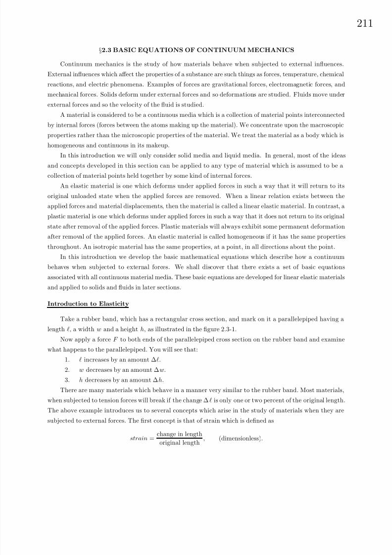
8/6/2019 Introduction to Tensor Calculus Continuum Mechanics - J. Heinbockel
http://slidepdf.com/reader/full/introduction-to-tensor-calculus-continuum-mechanics-j-heinbockel 217/372
21
§2.3 BASIC EQUATIONS OF CONTINUUM MECHANICS
Continuum mechanics is the study of how materials behave when subjected to external influences.
External influences which affect the properties of a substance are such things as forces, temperature, chemical
reactions, and electric phenomena. Examples of forces are gravitational forces, electromagnetic forces, and
mechanical forces. Solids deform under external forces and so deformations are studied. Fluids move underexternal forces and so the velocity of the fluid is studied.
A material is considered to be a continuous media which is a collection of material points interconnected
by internal forces (forces between the atoms making up the material). We concentrate upon the macroscopic
properties rather than the microscopic properties of the material. We treat the material as a body which is
homogeneous and continuous in its makeup.
In this introduction we will only consider solid media and liquid media. In general, most of the ideas
and concepts developed in this section can be applied to any type of material which is assumed to be a
collection of material points held together by some kind of internal forces.
An elastic material is one which deforms under applied forces in such a way that it will return to its
original unloaded state when the applied forces are removed. When a linear relation exists between the
applied forces and material displacements, then the material is called a linear elastic material. In contrast, a
plastic material is one which deforms under applied forces in such a way that it does not return to its original
state after removal of the applied forces. Plastic materials will always exhibit some permanent deformation
after removal of the applied forces. An elastic material is called homogeneous if it has the same properties
throughout. An isotropic material has the same properties, at a point, in all directions about the point.
In this introduction we develop the basic mathematical equations which describe how a continuum
behaves when subjected to external forces. We shall discover that there exists a set of basic equations
associated with all continuous material media. These basic equations are developed for linear elastic materials
and applied to solids and fluids in later sections.
Introduction to Elasticity
Take a rubber band, which has a rectangular cross section, and mark on it a parallelepiped having a
length , a width w and a height h, as illustrated in the figure 2.3-1.
Now apply a force F to both ends of the parallelepiped cross section on the rubber band and examine
what happens to the parallelepiped. You will see that:
1. increases by an amount ∆.
2. w decreases by an amount ∆w.
3. h decreases by an amount ∆h.
There are many materials which behave in a manner very similar to the rubber band. Most materials,
when subjected to tension forces will break if the change ∆ is only one or two percent of the original length.
The above example introduces us to several concepts which arise in the study of materials when they are
subjected to external forces. The first concept is that of strain which is defined as
strain =change in length
original length, (dimensionless).

8/6/2019 Introduction to Tensor Calculus Continuum Mechanics - J. Heinbockel
http://slidepdf.com/reader/full/introduction-to-tensor-calculus-continuum-mechanics-j-heinbockel 218/372

8/6/2019 Introduction to Tensor Calculus Continuum Mechanics - J. Heinbockel
http://slidepdf.com/reader/full/introduction-to-tensor-calculus-continuum-mechanics-j-heinbockel 219/372
21
Figure 2.3-2. Typical Stress-strain curve.
Consider a typical stress-strain curve, such as the one illustrated in the figure 2.3-2, which is obtained
by placing a material in the shape of a rod or wire in a machine capable of performing tensile straining at a
low rate. The engineering stress is the tensile force F divided by the original cross sectional area A0. Note
that during a tensile straining the cross sectional area A of the sample is continually changing and getting
smaller so that the actual stress will be larger than the engineering stress. Observe in the figure 2.3-2 that
the stress-strain relation remains linear up to a point labeled the proportional limit. For stress-strain points
in this linear region the Hooke’s law holds and the material will return to its original shape when the loading
is removed. For points beyond the proportional limit, but less than the yield point, the material no longer
obeys Hooke’s law. In this nonlinear region the material still returns to its original shape when the loading
is removed. The region beyond the yield point is called the plastic region. At the yield point and beyond,
there is a great deal of material deformation while the loading undergoes only small changes. For points
in this plastic region, the material undergoes a permanent deformation and does not return to its original
shape when the loading is removed. In the plastic region there usually occurs deformation due to slipping of
atomic planes within the material. In this introductory section we will restrict our discussions of materialstress-strain properties to the linear region.
EXAMPLE 2.3-1. (One dimensional elasticity) Consider a circular rod with cross sectional area A
which is subjected to an external force F applied to both ends. The figure 2.3-3 illustrates what happens to
the rod after the tension force F is applied. Consider two neighboring points P and Q on the rod, where P
is at the point x and Q is at the point x + ∆x. When the force F is applied to the rod it is stretched and
P moves to P and Q moves to Q. We assume that when F is applied to the rod there is a displacement
function u = u(x, t) which describes how each point in the rod moves as a function of time t. If we know the
displacement function u = u(x, t) we would then be able to calculate the following distances in terms of the
displacement function
P P = u(x, t), 0P = x + u(x, t), QQ = u(x + ∆x, t) 0Q = x + ∆x + u(x + ∆x, t).

8/6/2019 Introduction to Tensor Calculus Continuum Mechanics - J. Heinbockel
http://slidepdf.com/reader/full/introduction-to-tensor-calculus-continuum-mechanics-j-heinbockel 220/372
214
Figure 2.3-3. One dimensional rod subjected to tension force
The strain associated with the distance = ∆x = P Q is
e =∆
=
P Q − P Q
P Q=
(0Q − 0P )− (0Q− 0P )
P Q
e = [x + ∆x + u(x + ∆x, t) − (x + u(x, t))]− [(x + ∆x) − x]∆x
e =u(x + ∆x, t) − u(x, t)
∆x.
Use the Hooke’s law part(i) and write
F
A= E
u(x + ∆x, t) − u(x, t)
∆x.
Taking the limit as ∆x approaches zero we find that
F
A= E
∂u(x, t)
∂x.
Hence, the stress is proportional to the spatial derivative of the displacement function.
Normal and Shearing Stresses
Let us consider a more general situation in which we have some material which can be described as
having a surface area S which encloses a volume V. Assume that the density of the material is and the
material is homogeneous and isotropic. Further assume that the material is subjected to the forces b and t (n)
where b is a body force per unit mass [force/mass], and t (n) is a surface traction per unit area [force/area].
The superscript (n) on the vector is to remind you that we will only be interested in the normal component
of the surface forces. We will neglect body couples, surface couples, and concentrated forces or couples that
act at a single point. If the forces described above are everywhere continuous we can calculate the resultant
force F and resultant moment M acting on the material by constructing various surface and volume integrals
which sum the forces acting upon the material. In particular, the resultant force F acting on our material
can be described by the surface and volume integrals:
F =
S
t (n) dS +
V
b dτ (2.3.3)

8/6/2019 Introduction to Tensor Calculus Continuum Mechanics - J. Heinbockel
http://slidepdf.com/reader/full/introduction-to-tensor-calculus-continuum-mechanics-j-heinbockel 221/372
8/6/2019 Introduction to Tensor Calculus Continuum Mechanics - J. Heinbockel
http://slidepdf.com/reader/full/introduction-to-tensor-calculus-continuum-mechanics-j-heinbockel 222/372
216
Figure 2.3-5. Stress distribution at a point
For i = 1, 2, 3 we adopt the convention of sketching the components of t i in the positive directions if
the exterior normal to the surface xi = constant also points in the positive direction. This gives rise to the
figure 2.3-4 which illustrates the stress vectors acting upon an element of volume in rectangular Cartesian
coordinates. The components σ11, σ22, σ33 are called normal stresses while the components σij , i = j are
called shearing stresses. The equations (2.3.7) can be written in the more compact form using the indicial
notation as
t i = σij ej , i, j = 1, 2, 3. (2.3.8)
If we know the stress distribution at three orthogonal interfaces at a point P in a solid body, we can then
determine the stress at the point P with respect to any plane passing through the point P. With reference to
the figure 2.3-5, consider an arbitrary plane passing through the point P which lies within the material body
being considered. Construct the elemental tetrahedron with orthogonal axes parallel to the x1 = x, x2 = y
and x3 = z axes. In this figure we have the following surface tractions:
− t 1 on the surface 0BC
− t 2 on the surface 0AC
− t 3 on the surface 0AB
t (n) on the surface ABC
The superscript parenthesis n is to remind you that this surface traction depends upon the orientation of
the plane ABC which is determined by a unit normal vector having the direction cosines n1, n2 and n3.

8/6/2019 Introduction to Tensor Calculus Continuum Mechanics - J. Heinbockel
http://slidepdf.com/reader/full/introduction-to-tensor-calculus-continuum-mechanics-j-heinbockel 223/372
8/6/2019 Introduction to Tensor Calculus Continuum Mechanics - J. Heinbockel
http://slidepdf.com/reader/full/introduction-to-tensor-calculus-continuum-mechanics-j-heinbockel 224/372
218
Conservation of Linear Momentum
Let R denote a region in space where there exists a material volume with density having surface
tractions and body forces acting upon it. Let vi denote the velocity of the material volume and use Newton’s
second law to set the time rate of change of linear momentum equal to the forces acting upon the volume as
in (2.3.5). We find δ
δt
R
vj dτ
=
S
σij ni dS +
R
bj dτ.
Here dτ is an element of volume, dS is an element of surface area, bj are body forces per unit mass, and σij
are the stresses. Employing the Gauss divergence theorem, the surface integral term is replaced by a volume
integral and Newton’s second law is expressed in the form
R
f j − bj − σij
,i
dτ = 0, (2.3.16)
where f j is the acceleration from equation (1.4.54). Since R is an arbitrary region, the equation (2.3.16)
implies that
σij,i + bj = f j. (2.3.17)
This equation arises from a balance of linear momentum and represents the equations of motion for material
in a continuum. If there is no velocity term, then equation (2.3.17) reduces to an equilibrium equation which
can be written
σij,i + bj = 0. (2.3.18)
This equation can also be written in the covariant form
gsiσms,i + bm = 0,
which reduces to σij,j + bi = 0 in Cartesian coordinates. The equation (2.3.18) is an equilibrium equation
and is one of our fundamental equations describing a continuum.
Conservation of Angular Momentum
The conservation of angular momentum equation (2.3.6) has the Cartesian tensors representation
d
dt
R
eijk xj vk dτ
=
S
eijk xj σ pkn p dS +
R
eijk xj bk dτ. (2.3.19)
Employing the Gauss divergence theorem, the surface integral term is replaced by a volume integral to obtain
R
eijk d
dt(xj vk) − eijk
xj bk + ∂
∂x p(xj σ pk)
dτ = 0. (2.3.20)
Since equation (2.3.20) must hold for all arbitrary volumes R we conclude that
eijk d
dt(xj vk) = eijk
xj bk + xj
∂σ pk
∂x p+ σjk

8/6/2019 Introduction to Tensor Calculus Continuum Mechanics - J. Heinbockel
http://slidepdf.com/reader/full/introduction-to-tensor-calculus-continuum-mechanics-j-heinbockel 225/372
21
Figure 2.3-6. Shearing parallel to the y axis
which can be rewritten in the form
eijk
σjk + xj (
∂σ pk
∂x p+ bk −
dvk
dt) − vj vk
= 0. (2.3.21)
In the equation (2.3.21) the middle term is zero because of the equation (2.3.17). Also the last term in(2.3.21) is zero because eijk vj vk represents the cross product of a vector with itself. The equation (2.3.21)
therefore reduces to
eijk σjk = 0, (2.3.22)
which implies (see exercise 1.1, problem 22) that σij = σji for all i and j. Thus, the conservation of angular
momentum requires that the stress tensor be symmetric. Consequently, there are only 6 independent stress
components to be determined. This is another fundamental law for a continuum.
Strain in Two Dimensions
Consider the matrix equation xy
=
1 0β 1
xy
(2.3.23)
which can be used to transform points (x, y) to points (x, y). When this transformation is applied to the
unit square illustrated in the figure 2.3-6(a) we obtain the geometry illustrated in the figure 2.3-6(b) which
represents a shearing parallel to the y axis. If β is very small, we can use the approximation tan β ≈ β and
then this transformation can be thought of as a rotation of the element P 1P 2 through an angle β to the
position P 1P 2 when the barred axes are placed atop the unbarred axes.
Similarly, the matrix equation xy
=
1 α0 1
xy
(2.3.24)
can be used to represent a shearing of the unit square parallel to the x axis as illustrated in the figure
2.3-7(b).

8/6/2019 Introduction to Tensor Calculus Continuum Mechanics - J. Heinbockel
http://slidepdf.com/reader/full/introduction-to-tensor-calculus-continuum-mechanics-j-heinbockel 226/372
220
Figure 2.3-7. Shearing parallel to the x axis
Figure 2.3-8. Shearing parallel to x and y axes
Again, if α is very small, we may use the approximation tan α ≈ α and interpret α as an angular rotation
of the element P 1P 4 to the position P 1P 4. Now let us multiply the matrices given in equations (2.3.23) and
(2.3.24). Note that the order of multiplication is important as can be seen by an examination of the products
xy
=
1 0β 1
1 α0 1
xy
=
1 αβ 1 + αβ
xy
xy
=
1 α0 1
1 0β 1
xy
=
1 + αβ α
β 1
xy
.
(2.3.25)
In equation (2.3.25) we will assume that the product αβ is very, very small and can be neglected. Then the
order of matrix multiplication will be immaterial and the transformation equation (2.3.25) will reduce to
xy
=
1 αβ 1
xy
. (2.3.26)
Applying this transformation to our unit square we obtain the simultaneous shearing parallel to both the xand y axes as illustrated in the figure 2.3-8.
This transformation can then be interpreted as the superposition of the two shearing elements depicted
in the figure 2.3-9.
For comparison, we consider also the transformation equation
xy
=
1 0−α 1
xy
(2.3.27)

8/6/2019 Introduction to Tensor Calculus Continuum Mechanics - J. Heinbockel
http://slidepdf.com/reader/full/introduction-to-tensor-calculus-continuum-mechanics-j-heinbockel 227/372
22
Figure 2.3-9. Superposition of shearing elements
Figure 2.3-10. Rotation of element P 1P 2
where α is very small. Applying this transformation to the unit square previously considered we obtain the
results illustrated in the figure 2.3-10.Note the difference in the direction of shearing associated with the transformation equations (2.3.27)
and (2.3.23) illustrated in the figures 2.3-6 and 2.3-10. If the matrices appearing in the equations (2.3.24)
and (2.3.27) are multiplied and we neglect product terms because α is assumed to be very small, we obtain
the matrix equation
xy
=
1 α−α 1
xy
=
1 00 1
xy
identity
+
0 α−α 0
xy
rotation
. (2.3.28)
This can be interpreted as a superposition of the transformation equations (2.3.24) and (2.3.27) which
represents a rotation of the unit square as illustrated in the figure 2.3-11.
The matrix on the right-hand side of equation (2.3.28) is referred to as a rotation matrix. The ideas
illustrated by the above simple transformations will appear again when we consider the transformation of an
arbitrary small element in a continuum when it under goes a strain. In particular, we will be interested in
extracting the rigid body rotation from a deformed element and treating this rotation separately from the
strain displacement.
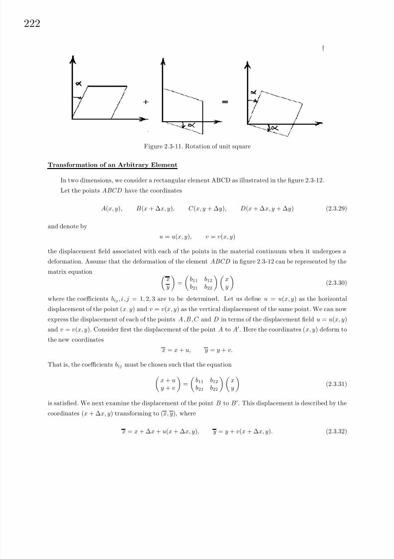
8/6/2019 Introduction to Tensor Calculus Continuum Mechanics - J. Heinbockel
http://slidepdf.com/reader/full/introduction-to-tensor-calculus-continuum-mechanics-j-heinbockel 228/372
222
Figure 2.3-11. Rotation of unit square
Transformation of an Arbitrary Element
In two dimensions, we consider a rectangular element ABCD as illustrated in the figure 2.3-12.
Let the points ABCD have the coordinates
A(x, y), B(x + ∆x, y), C (x, y + ∆y), D(x + ∆x, y + ∆y) (2.3.29)
and denote by
u = u(x, y), v = v(x, y)
the displacement field associated with each of the points in the material continuum when it undergoes a
deformation. Assume that the deformation of the element ABCD in figure 2.3-12 can be represented by the
matrix equation xy
=
b11 b12
b21 b22
xy
(2.3.30)
where the coefficients bij , i , j = 1, 2, 3 are to be determined. Let us define u = u(x, y) as the horizontal
displacement of the point (x, y) and v = v(x, y) as the vertical displacement of the same point. We can now
express the displacement of each of the points A , B, C and D in terms of the displacement field u = u(x, y)
and v = v(x, y). Consider first the displacement of the point A to A. Here the coordinates (x, y) deform to
the new coordinates
x = x + u, y = y + v.
That is, the coefficients bij must be chosen such that the equation
x + uy + v =
b11 b12
b21 b22 xy (2.3.31)
is satisfied. We next examine the displacement of the point B to B. This displacement is described by the
coordinates (x + ∆x, y) transforming to (x, y), where
x = x + ∆x + u(x + ∆x, y), y = y + v(x + ∆x, y). (2.3.32)

8/6/2019 Introduction to Tensor Calculus Continuum Mechanics - J. Heinbockel
http://slidepdf.com/reader/full/introduction-to-tensor-calculus-continuum-mechanics-j-heinbockel 229/372
22
Figure 2.3-12. Displacement of element ABCD to ABC D
Expanding u and v in (2.3.32) in Taylor series about the point (x, y) we find
x = x + ∆x + u +
∂u
∂x ∆x + h.o.t.
y = y + v +∂v
∂x∆x + h.o.t.,
(2.3.33)
where h.o.t. denotes higher order terms which have been neglected. The equations (2.3.33) require that the
coefficients bij satisfy the matrix equation
x + u + ∆x + ∂u
∂x∆x
y + v + ∂v∂x
∆x
=
b11 b12
b21 b22
x + ∆x
y
. (2.3.34)
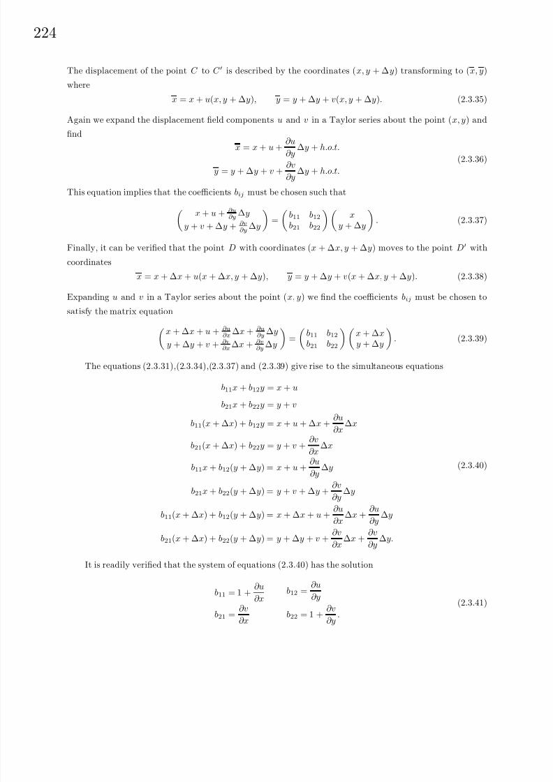
8/6/2019 Introduction to Tensor Calculus Continuum Mechanics - J. Heinbockel
http://slidepdf.com/reader/full/introduction-to-tensor-calculus-continuum-mechanics-j-heinbockel 230/372
224
The displacement of the point C to C is described by the coordinates (x, y + ∆y) transforming to (x, y)
where
x = x + u(x, y + ∆y), y = y + ∆y + v(x, y + ∆y). (2.3.35)
Again we expand the displacement field components u and v in a Taylor series about the point (x, y) and
findx = x + u +
∂u
∂y∆y + h.o.t.
y = y + ∆y + v +∂v
∂y∆y + h.o.t.
(2.3.36)
This equation implies that the coefficients bij must be chosen such that
x + u + ∂u
∂y∆y
y + v + ∆y + ∂v∂y
∆y
=
b11 b12
b21 b22
x
y + ∆y
. (2.3.37)
Finally, it can be verified that the point D with coordinates (x + ∆x, y + ∆y) moves to the point D with
coordinates
x = x + ∆x + u(x + ∆x, y + ∆y), y = y + ∆y + v(x + ∆x, y + ∆y). (2.3.38)
Expanding u and v in a Taylor series about the point (x, y) we find the coefficients bij must be chosen to
satisfy the matrix equation
x + ∆x + u + ∂u
∂x∆x + ∂u
∂y∆y
y + ∆y + v + ∂v∂x
∆x + ∂v∂y
∆y
=
b11 b12
b21 b22
x + ∆xy + ∆y
. (2.3.39)
The equations (2.3.31),(2.3.34),(2.3.37) and (2.3.39) give rise to the simultaneous equations
b11x + b12y = x + u
b21x + b22y = y + v
b11(x + ∆x) + b12y = x + u + ∆x +∂u
∂x∆x
b21(x + ∆x) + b22y = y + v +∂v
∂x∆x
b11x + b12(y + ∆y) = x + u +∂u
∂y∆y
b21x + b22(y + ∆y) = y + v + ∆y +∂v
∂y∆y
b11(x + ∆x) + b12(y + ∆y) = x + ∆x + u +∂u
∂x∆x +
∂u
∂y∆y
b21(x + ∆x) + b22(y + ∆y) = y + ∆y + v +∂v
∂x
∆x +∂v
∂y
∆y.
(2.3.40)
It is readily verified that the system of equations (2.3.40) has the solution
b11 = 1 +∂u
∂x
b21 =∂v
∂x
b12 =∂u
∂y
b22 = 1 +∂v
∂y.
(2.3.41)
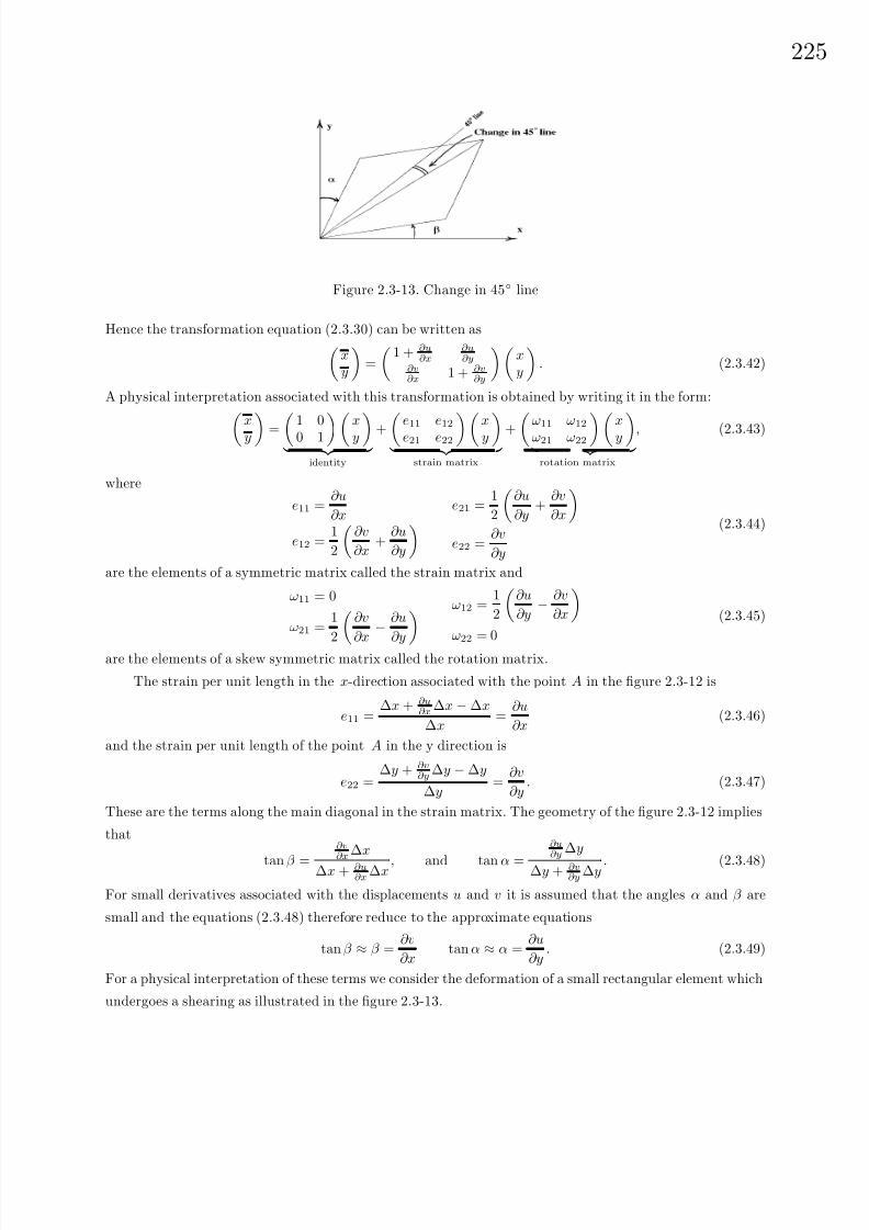
8/6/2019 Introduction to Tensor Calculus Continuum Mechanics - J. Heinbockel
http://slidepdf.com/reader/full/introduction-to-tensor-calculus-continuum-mechanics-j-heinbockel 231/372
22
Figure 2.3-13. Change in 45 line
Hence the transformation equation (2.3.30) can be written asxy
=
1 + ∂u
∂x∂u∂y
∂v∂x
1 + ∂v∂y
xy
. (2.3.42)
A physical interpretation associated with this transformation is obtained by writing it in the form:
xy = 1 0
0 1 xy
identity
+ e11 e12
e21 e22x
y strain matrix
+ ω11 ω12
ω21 ω22x
y rotation matrix
, (2.3.43)
where
e11 =∂u
∂x
e12 =1
2
∂v
∂x+
∂u
∂y
e21 =1
2
∂u
∂y+
∂v
∂x
e22 =∂v
∂y
(2.3.44)
are the elements of a symmetric matrix called the strain matrix and
ω11 = 0
ω21 =1
2
∂v
∂x− ∂u
∂y
ω12 =1
2
∂u
∂y− ∂v
∂x
ω22 = 0
(2.3.45)
are the elements of a skew symmetric matrix called the rotation matrix.
The strain per unit length in the x-direction associated with the point A in the figure 2.3-12 is
e11 =∆x + ∂u
∂x∆x − ∆x
∆x=
∂u
∂x(2.3.46)
and the strain per unit length of the point A in the y direction is
e22 =∆y + ∂v
∂y∆y − ∆y
∆y=
∂v
∂y. (2.3.47)
These are the terms along the main diagonal in the strain matrix. The geometry of the figure 2.3-12 implies
that
tan β =
∂v∂x
∆x
∆x + ∂u∂x
∆x , and tan α =
∂u∂y
∆y
∆y + ∂v∂y
∆y . (2.3.48)
For small derivatives associated with the displacements u and v it is assumed that the angles α and β are
small and the equations (2.3.48) therefore reduce to the approximate equations
tan β ≈ β =∂v
∂xtan α ≈ α =
∂u
∂y. (2.3.49)
For a physical interpretation of these terms we consider the deformation of a small rectangular element which
undergoes a shearing as illustrated in the figure 2.3-13.

8/6/2019 Introduction to Tensor Calculus Continuum Mechanics - J. Heinbockel
http://slidepdf.com/reader/full/introduction-to-tensor-calculus-continuum-mechanics-j-heinbockel 232/372
226
Figure 2.3-14. Displacement field due to state of strain
The quantity
α + β =
∂u
∂y+
∂v
∂x
= 2e12 = 2e21 (2.3.50)
is the change from a ninety degree angle due to the deformation and hence we can write 12 (α + β ) = e12 = e21
as representing a change from a 45 angle due to the deformation. The quantities e21, e12 are called the
shear strains and the quantity
γ 12 = 2e12 (2.3.51)
is called the shear angle.
In the equation (2.3.45), the quantities ω21 = −ω12 are the elements of the rigid body rotation matrix
and are interpreted as angles associated with a rotation. The situation is analogous to the transformations
and figures for the deformation of the unit square which was considered earlier.
Strain in Three Dimensions
The development of strain in three dimensions is approached from two different viewpoints. The first
approach considers the derivation using Cartesian tensors and the second approach considers the derivation
of strain using generalized tensors.
Cartesian Tensor Derivation of Strain.
Consider a material which is subjected to external forces such that all the points in the material undergo
a deformation. Let (y1, y2, y3) denote a set of orthogonal Cartesian coordinates, fixed in space, which is
used to describe the deformations within the material. Further, let ui = ui(y1, y2, y3), i = 1, 2, 3 denote a
displacement field which describes the displacement of each point within the material. With reference to thefigure 2.3-14 let P and Q denote two neighboring points within the material while it is in an unstrained state.
These points move to the points P and Q when the material is in a state of strain. We let yi, i = 1, 2, 3
represent the position vector to the general point P in the material, which is in an unstrained state, and
denote by yi + ui, i = 1, 2, 3 the position vector of the point P when the material is in a state of strain.

8/6/2019 Introduction to Tensor Calculus Continuum Mechanics - J. Heinbockel
http://slidepdf.com/reader/full/introduction-to-tensor-calculus-continuum-mechanics-j-heinbockel 233/372
22
For Q a neighboring point of P which moves to Q when the material is in a state of strain, we have
from the figure 2.3-14 the following vectors:
position of P : yi, i = 1, 2, 3
position of P : yi + ui(y1, y2, y3), i = 1, 2, 3
position of Q : yi + ∆yi, i = 1, 2, 3position of Q : yi + ∆yi + ui(y1 + ∆y1, y2 + ∆y2, y3 + ∆y3), i = 1, 2, 3
(2.3.52)
Employing our earlier one dimensional definition of strain, we define the strain associated with the point P
in the direction P Q as e =L − L0
L0, where L0 = P Q and L = P Q. To calculate the strain we need to first
calculate the distances L0 and L. The quantities L20 and L2 are easily calculated by considering dot products
of vectors. For example, we have L20 = ∆yi∆yi, and the distance L = P Q is the magnitude of the vector
yi + ∆yi + ui(y1 + ∆y1, y2 + ∆y2, y3 + ∆y3) − (yi + ui(y1, y2, y3)), i = 1, 2, 3.
Expanding the quantity ui(y1 + ∆y1, y2 + ∆y2, y3 + ∆y3) in a Taylor series about the point P and neglecting
higher order terms of the expansion we find that
L2 = (∆yi +∂ui
∂ym
∆ym)(∆yi +∂ui
∂yn
∆yn).
Expanding the terms in this expression produces the equation
L2 = ∆yi∆yi +∂ui
∂yn
∆yi∆yn +∂ui
∂ym
∆ym∆yi +∂ui
∂ym
∂ui
∂yn
∆ym∆yn.
Note that L and L0 are very small and so we express the difference L2 −L20 in terms of the strain e. We can
write
L2 − L20 = (L + L0)(L − L0) = (L − L0 + 2L0)(L − L0) = (e + 2)eL2
0.
Now for e very small, and e2 negligible, the above equation produces the approximation
eL20 ≈ L2 − L20
2= 1
2
∂um
∂yn
+ ∂un
∂ym
+ ∂ur
∂ym
∂ur
∂yn
∆ym∆yn.
The quantities
emn =1
2
∂um
∂yn
+∂un
∂ym
+∂ur
∂ym
∂ur
∂yn
(2.3.53)
is called the Green strain tensor or Lagrangian strain tensor. To show that eij is indeed a tensor, we consider
the transformation yi = ijyj +bi, where ji ki = δjk = ij ik. Note that from the derivative relation ∂yi∂yj
= ij
and the transformation equations ui = ij uj, i = 1, 2, 3 we can express the strain in the barred system of
coordinates. Performing the necessary calculations produces
eij =1
2 ∂ui
∂yj
+∂uj
∂yi
+∂ur
∂y i
∂ur
∂yj =
1
2
∂
∂yn
(ikuk)∂yn
∂yj
+∂
∂ym
(jk uk)∂ym
∂yi
+∂
∂yk
(rsus)∂yk
∂y i
∂
∂yt
(rmum)∂yt
∂y j
=1
2
imnj
∂um
∂yn
+ jk mi
∂uk
∂ym
+ rsrpkitj
∂us
∂yk
∂u p
∂yt
=1
2
∂um
∂yn
+∂un
∂ym
+∂us
∂ym
∂us
∂yn
imnj
or eij = emnimnj .Consequently, the strain eij transforms like a second order Cartesian tensor.

8/6/2019 Introduction to Tensor Calculus Continuum Mechanics - J. Heinbockel
http://slidepdf.com/reader/full/introduction-to-tensor-calculus-continuum-mechanics-j-heinbockel 234/372
228
Lagrangian and Eulerian Systems
Let xi denote the initial position of a material particle in a continuum. Assume that at a later time the
particle has moved to another point whose coordinates are xi. Both sets of coordinates are referred to the
same coordinate system. When the final position can be expressed as a function of the initial position and
time we can write xi = xi(x1, x2, x3, t). Whenever the changes of any physical quantity is represented in terms
of its initial position and time, the representation is referred to as a Lagrangian or material representation of
the quantity. This can be thought of as a transformation of the coordinates. When the Jacobian J ( xx
) of this
transformation is different from zero, the above set of equations have a unique inverse xi = xi(x1, x2, x3, t),
where the position of the particle is now expressed in terms of its instantaneous position and time. Such a
representation is referred to as an Eulerian or spatial description of the motion.
Let (x1, x2, x3) denote the initial position of a particle whose motion is described by xi = xi(x1, x2, x3, t),
then ui = xi − xi denotes the displacement vector which can by represented in a Lagrangian or Eulerian
form. For example, if x1 = 2(x1 − x2)(et − 1) + (x2 − x1)(e−t − 1) + x1
x2 = (x1 − x2)(et
− 1) + (x2 − x1)(e−t
− 1) + x2
x3 = x3
then the displacement vector can be represented in the Lagrangian form
u1 = 2(x1 − x2)(et − 1) + (x2 − x1)(e−t − 1)
u2 = (x1 − x2)(et − 1) + (x2 − x1)(e−t − 1)
u3 = 0
or the Eulerian form
u1 = x1
−(2x2
−x1)(1
−e−t)
−(x1
−x2)(e−2t
−e−t)
−x1e−t
u2 = x2 − (2x2 − x1)(1− e−t) − (x2 − x1)(e−2t − e−t) − x2e−t
u3 = 0.
Note that in the Lagrangian system the displacements are expressed in terms of the initial position and
time, while in the Eulerian system the independent variables are the position coordinates and time. Euler
equations describe, as a function of time, how such things as density, pressure, and fluid velocity change at
a fixed point in the medium. In contrast, the Lagrangian viewpoint follows the time history of a moving
individual fluid particle as it moves through the medium.
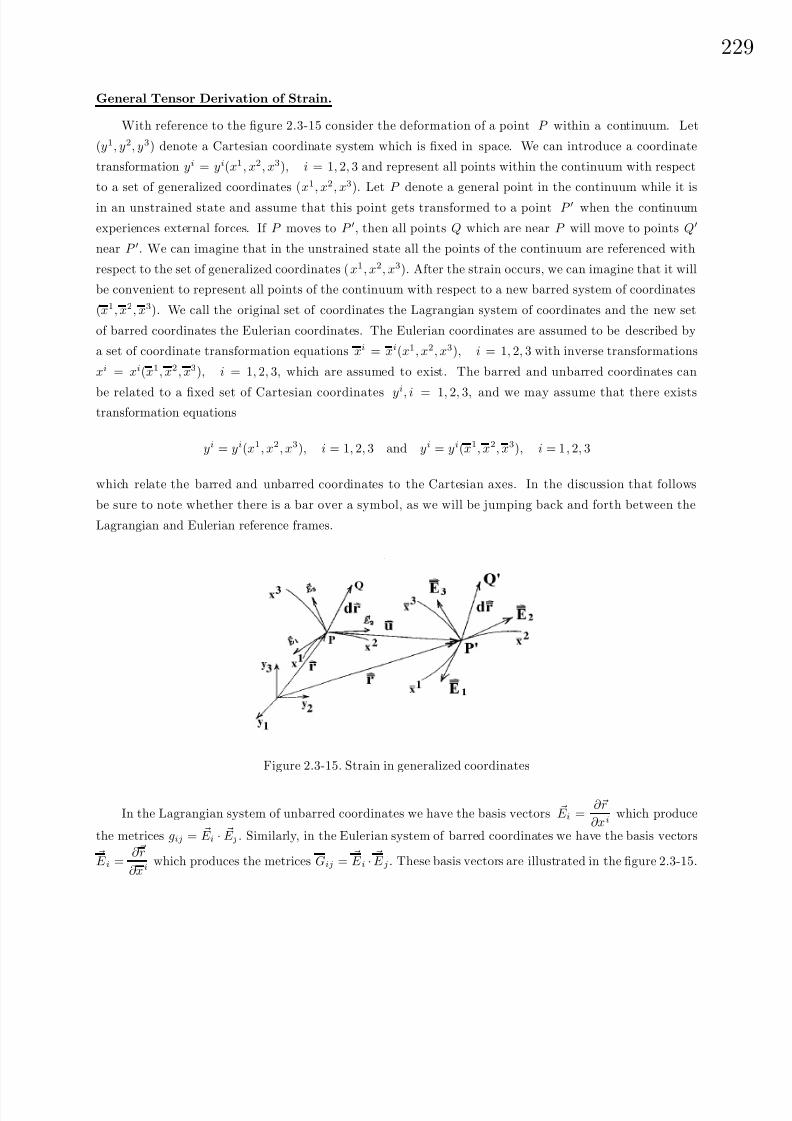
8/6/2019 Introduction to Tensor Calculus Continuum Mechanics - J. Heinbockel
http://slidepdf.com/reader/full/introduction-to-tensor-calculus-continuum-mechanics-j-heinbockel 235/372
22
General Tensor Derivation of Strain.
With reference to the figure 2.3-15 consider the deformation of a point P within a continuum. Let
(y1, y2, y3) denote a Cartesian coordinate system which is fixed in space. We can introduce a coordinate
transformation yi = yi(x1, x2, x3), i = 1, 2, 3 and represent all points within the continuum with respect
to a set of generalized coordinates (x1, x2, x3). Let P denote a general point in the continuum while it is
in an unstrained state and assume that this point gets transformed to a point P when the continuum
experiences external forces. If P moves to P , then all points Q which are near P will move to points Q
near P . We can imagine that in the unstrained state all the points of the continuum are referenced with
respect to the set of generalized coordinates (x1, x2, x3). After the strain occurs, we can imagine that it will
be convenient to represent all points of the continuum with respect to a new barred system of coordinates
(x1, x2, x3). We call the original set of coordinates the Lagrangian system of coordinates and the new set
of barred coordinates the Eulerian coordinates. The Eulerian coordinates are assumed to be described by
a set of coordinate transformation equations xi = xi(x1, x2, x3), i = 1, 2, 3 with inverse transformations
xi = xi(x1, x2, x3), i = 1, 2, 3, which are assumed to exist. The barred and unbarred coordinates can
be related to a fixed set of Cartesian coordinates yi, i = 1, 2, 3, and we may assume that there existstransformation equations
yi = yi(x1, x2, x3), i = 1, 2, 3 and yi = yi(x1, x2, x3), i = 1, 2, 3
which relate the barred and unbarred coordinates to the Cartesian axes. In the discussion that follows
be sure to note whether there is a bar over a symbol, as we will be jumping back and forth between the
Lagrangian and Eulerian reference frames.
Figure 2.3-15. Strain in generalized coordinates
In the Lagrangian system of unbarred coordinates we have the basis vectors E i =∂r
∂xiwhich produce
the metrices gij = E i · E j . Similarly, in the Eulerian system of barred coordinates we have the basis vectors
E i =∂ r
∂xiwhich produces the metrices Gij = E i · E j . These basis vectors are illustrated in the figure 2.3-15.
8/6/2019 Introduction to Tensor Calculus Continuum Mechanics - J. Heinbockel
http://slidepdf.com/reader/full/introduction-to-tensor-calculus-continuum-mechanics-j-heinbockel 236/372
230
We assume that an element of arc length squared ds2 in the unstrained state is deformed to the element
of arc length squared ds2 in the strained state. An element of arc length squared can be expressed in terms
of the barred or unbarred coordinates. For example, in the Lagrangian system, let dr = P Q so that
L20 = dr · dr = ds2 = gij dxidxj , (2.3.54)
where gij are the metrices in the Lagrangian coordinate system. This same element of arc length squared
can be expressed in the barred system by
L20 = ds2 = gij dxidxj , where gij = gmn
∂xm
∂xi
∂xn
∂xj. (2.3.55)
Similarly, in the Eulerian system of coordinates the deformed arc length squared is
L2 = d r · d r = ds2 = Gij dxidxj , (2.3.56)
where Gij are the metrices in the Eulerian system of coordinates. This same element of arc length squared
can be expressed in the Lagrangian system by the relation
L2 = ds2 = Gij dxidxj , where Gij = Gmn
∂xm
∂xi
∂xn
∂xj. (2.3.57)
In the Lagrangian system we have
ds2 − ds2 = (Gij − gij)dxidxj = 2eij dxidxj
where
eij =1
2(Gij − gij) (2.3.58)
is called the Green strain tensor or Lagrangian strain tensor. Alternatively, in the Eulerian system of
coordinates we may write
ds2 − ds2 =
Gij − gij
dxidxj = 2eijdxidxj
where
eij =1
2
Gij − gij
(2.3.59)
is called the Almansi strain tensor or Eulerian strain tensor.

8/6/2019 Introduction to Tensor Calculus Continuum Mechanics - J. Heinbockel
http://slidepdf.com/reader/full/introduction-to-tensor-calculus-continuum-mechanics-j-heinbockel 237/372
23
Note also in the figure 2.3-15 there is the displacement vector u. This vector can be represented in any
of the following forms:
u = ui E i contravariant, Lagrangian basis
u = ui E i covariant, Lagrangian reciprocal basis
u = ui E i contravariant, Eulerian basis
u = ui
E
icovariant, Eulerian reciprocal basis.
By vector addition we have r + u = r and consequently dr + du = d r. In the Lagrangian frame of reference
at the point P we represent u in the contravariant form u = ui E i and write dr in the form dr = dxi E i. By
use of the equation (1.4.48) we can express du in the form du = ui,kdxk E i. These substitutions produce the
representation d r = (dxi + ui,kdxk) E i in the Lagrangian coordinate system. We can then express ds2 in the
Lagrangian system. We find
d r · d r = ds2 = (dxi + ui,kdxk) E i · (dxj + uj
,mdxm) E j
= (dxi
dxj
+ uj
,mdxm
dxi
+ ui
,kdxk
dxj
+ ui
,kuj
,mdxk
dxm
)gij
and consequently from the relation (2.3.58) we derive the representation
eij =1
2
ui,j + uj,i + um,ium
,j
. (2.3.60)
This is the representation of the Lagrangian strain tensor in any system of coordinates. The strain tensor
eij is symmetric. We will restrict our study to small deformations and neglect the product terms in equation
(2.3.60). Under these conditions the equation (2.3.60) reduces to eij = 12 (ui,j + uj,i).
If instead, we chose to represent the displacement u with respect to the Eulerian basis, then we can
write
u = u
i
E i with du = u
i
,kdx
k
E i.
These relations imply that
dr = d r − du = (dxi − ui,kdxk) E i.
This representation of dr in the Eulerian frame of reference can be used to calculate the strain eij from the
relation ds2 − ds2. It is left as an exercise to show that there results
eij =1
2
ui,j + uj,i − um,ium
,j
. (2.3.61)
The equation (2.3.61) is the representation of the Eulerian strain tensor in any system of coordinates. Under
conditions of small deformations both the equations (2.3.60) and (2.3.61) reduce to the linearized Lagrangian
and Eulerian strain tensor eij = 12 (ui,j + uj,i). In the case of large deformations the equations (2.3.60) and(2.3.61) describe the strains. In the case of linear elasticity, where the deformations are very small, the
product terms in equations (2.3.60) and (2.3.61) are neglected and the Lagrangian and Eulerian strains
reduce to their linearized forms
eij =1
2[ui,j + uj,i] eij =
1
2[ui,j + uj,i] . (2.3.62)

8/6/2019 Introduction to Tensor Calculus Continuum Mechanics - J. Heinbockel
http://slidepdf.com/reader/full/introduction-to-tensor-calculus-continuum-mechanics-j-heinbockel 238/372
232
Figure 2.3-16. Displacement due to strain
Compressible and Incompressible Material With reference to figure 2.3-16, let xi, i = 1, 2, 3 denote
the position vector of an arbitrary point P in a continuum before there is a state of strain. Let Q be
a neighboring point of P with position vector xi + dxi, i = 1, 2, 3. Also in the figure 2.3-16 there is the
displacement vector u. Here it is assumed that u = u(x1, x2, x3) denotes the displacement field when the
continuum is in a state of strain. The figure 2.3-16 illustrates that in a state of strain P moves to P and Q
moves to Q. Let us find a relationship between the distance P Q before the strain and the distance P Q when
the continuum is in a state of strain. For E 1, E 2, E 3 basis functions constructed at P we have previously
shown that if
u(x1, x2, x3) = ui E i then du = ui,j dxj E i.
Now for u + du the displacement of the point Q we may use vector addition and write
P Q + u + du = u + P Q. (2.3.63)
Let P Q = dxi
E i = ai
E i denote an arbitrary small change in the continuum. This arbitrary displacementgets deformed to P Q = Ai E i due to the state of strain in the continuum. Employing the equation (2.3.63)
we write
dxi + ui,j dxj = ai + ui
,j aj = Ai
which can be written in the form
δai = Ai − ai = ui,j aj where dxi = ai, i = 1, 2, 3 (2.3.64)
denotes an arbitrary small change. The tensor ui,j and the associated tensor ui,j = gitut
,j are in general
not symmetric tensors. However, we know we can express ui,j as the sum of a symmetric (eij ) and skew-
symmetric(ωij) tensor. We therefore write
ui,j = eij + ωij or ui,j = ei
j + ωij ,
where
eij =1
2(ui,j + uj,i) =
1
2(gimum
,j + gjmum,i) and ωij =
1
2(ui,j − uj,i) =
1
2(gimum
,j − gjmum,i) .
The deformation of a small quantity ai can therefore be represented by a pure strain Ai − ai = eisas followed
by a rotation Ai − ai = ωisas.
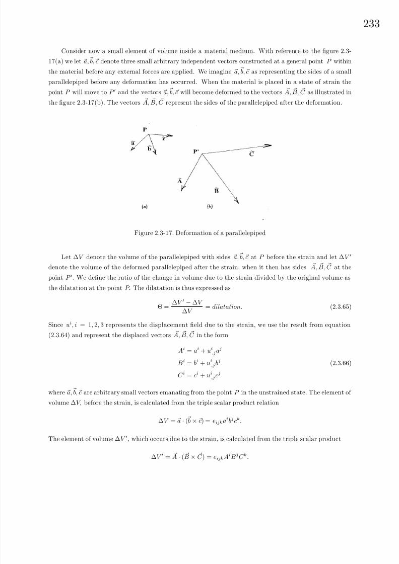
8/6/2019 Introduction to Tensor Calculus Continuum Mechanics - J. Heinbockel
http://slidepdf.com/reader/full/introduction-to-tensor-calculus-continuum-mechanics-j-heinbockel 239/372
23
Consider now a small element of volume inside a material medium. With reference to the figure 2.3-
17(a) we let a, b, c denote three small arbitrary independent vectors constructed at a general point P within
the material before any external forces are applied. We imagine a, b, c as representing the sides of a small
parallelepiped before any deformation has occurred. When the material is placed in a state of strain the
point P will move to P and the vectors a, b, c will become deformed to the vectors A, B, C as illustrated in
the figure 2.3-17(b). The vectors A, B, C represent the sides of the parallelepiped after the deformation.
Figure 2.3-17. Deformation of a parallelepiped
Let ∆V denote the volume of the parallelepiped with sides a, b, c at P before the strain and let ∆V
denote the volume of the deformed parallelepiped after the strain, when it then has sides A, B, C at the
point P . We define the ratio of the change in volume due to the strain divided by the original volume as
the dilatation at the point P. The dilatation is thus expressed as
Θ =∆V − ∆V
∆V = dilatation. (2.3.65)
Since ui, i = 1, 2, 3 represents the displacement field due to the strain, we use the result from equation
(2.3.64) and represent the displaced vectors A, B, C in the form
Ai = ai + ui,j aj
Bi = bi + ui,j bj
C i = ci + ui,j cj
(2.3.66)
where a, b, c are arbitrary small vectors emanating from the point P in the unstrained state. The element of
volume ∆V, before the strain, is calculated from the triple scalar product relation
∆V = a · ( b × c) = eijk aibj ck.
The element of volume ∆V , which occurs due to the strain, is calculated from the triple scalar product
∆V = A · ( B × C ) = eijk AiBj C k.

8/6/2019 Introduction to Tensor Calculus Continuum Mechanics - J. Heinbockel
http://slidepdf.com/reader/full/introduction-to-tensor-calculus-continuum-mechanics-j-heinbockel 240/372
234
Substituting the relations from the equations (2.3.66) into the triple scalar product gives
∆V = eijk (ai + ui,mam)(bj + uj
,nbn)(ck + uk,pc p).
Expanding the triple scalar product and employing the result from Exercise 1.4, problem 34, we find the
simplified result gives us the dilatation
Θ =∆V − ∆V
∆V = ur
,r = div (u). (2.3.67)
That is, the dilatation is the divergence of the displacement field. If the divergence of the displacement field
is zero, there is no volume change and the material is said to be incompressible. If the divergence of the
displacement field is different from zero, the material is said to be compressible.
Note that the strain eij is expressible in terms of the displacement field by the relation
eij =1
2(ui,j + uj,i), and consequently gmnemn = ur
,r . (2.3.68)
Hence, for an orthogonal system of coordinates the dilatation can be expressed in terms of the strain elementsalong the main diagonal.
Conservation of Mass
Consider the material in an arbitrary region R of a continuum. Let = (x, y, z, t) denote the density
of the material within the region. Assume that the dimension of the density is gm/cm3 in the cgs system
of units. We shall assume that the region R is bounded by a closed surface S with exterior unit normal n
defined everywhere on the surface. Further, we let v = v(x, y, z, t) denote a velocity field associated with all
points within the continuum. The velocity field has units of cm/sec in the cgs system of units. Neglecting
sources and sinks, the law of conservation of mass examines all the material entering and leaving a region R.
Enclosed within R is the material mass m where m =
R
dτ with dimensions of gm in the cgs system of
units. Here dτ denotes an element of volume inside the region R. The change of mass with time is obtained
by differentiating the above relation. Differentiating the mass produces the equation
∂m
∂t=
R
∂
∂tdτ (2.3.69)
and has the dimensions of gm/sec.
Consider also the surface integral
I =
S
v · n dσ (2.3.70)
where dσ is an element of surface area on the surface S which encloses R and n is the exterior unit normalvector to the surface S. The dimensions of the integral I is determined by examining the dimensions of each
term in the integrand of I. We find that
[I ] =gm
cm3· cm
sec· cm2 =
gm
sec
and so the dimension of I is the same as the dimensions for the change of mass within the region R. The
surface integral I is the flux rate of material crossing the surface of R and represents the change of mass

8/6/2019 Introduction to Tensor Calculus Continuum Mechanics - J. Heinbockel
http://slidepdf.com/reader/full/introduction-to-tensor-calculus-continuum-mechanics-j-heinbockel 241/372
23
entering the region if v · n is negative and the change of mass leaving the region if v · n is positive, as n is
always an exterior unit normal vector. Equating the relations from equations (2.3.69) and (2.3.70) we obtain
a mathematical statement for mass conservation
∂m
∂t=
R
∂
∂tdτ = −
S
v · n dσ. (2.3.71)
The equation (2.3.71) implies that the rate at which the mass contained in R increases must equal the rate
at which the mass flows into R through the surface S. The negative sign changes the direction of the exterior
normal so that we consider flow of material into the region. Employing the Gauss divergence theorem, the
surface integral in equation (2.3.71) can be replaced by a volume integral and the law of conservation of
mass is then expressible in the form
R
∂
∂t+ div (v)
dτ = 0. (2.3.72)
Since the region R is an arbitrary volume we conclude that the term inside the brackets must equal zero.
This gives us the continuity equation∂
∂t+ div (v) = 0 (2.3.73)
which represents the mass conservation law in terms of velocity components. This is the Eulerian represen-
tation of continuity of mass flow.
Equivalent forms of the continuity equation are:
∂
∂t+ v · grad + div v = 0
∂
∂t+ vi
∂
∂xi+
∂vi
∂xi= 0
D
Dt +
∂vi
∂xi = 0
whereD
Dt=
∂
∂t+
∂
∂xi
dxi
dt=
∂
∂t+
∂
∂xivi is called the material derivative of the density . Note that the
material derivative contains the expression ∂∂xi
vi which is known as the convective or advection term. If the
density = (x, y, z, t) is a constant we have
D
Dt=
∂
∂t+
∂
∂x
dx
dt+
∂
∂y
dy
dt+
∂
∂z
dz
dt=
∂
∂t+
∂
∂xi
dxi
dt= 0 (2.3.74)
and hence the continuity equation reduces to div (v) = 0. Thus, if div (v) is zero, then the material is
incompressible.
EXAMPLE 2.3-2. (Continuity Equation) Find the Lagrangian representation of mass conservation.
Solution: Let (X, Y, Z ) denote the initial position of a fluid particle and denote the density of the fluid by
(X, Y, Z, t) so that (X,Y,Z, 0) denotes the density at the time t = 0. Consider a simple closed region in
our continuum and denote this region by R(0) at time t = 0 and by R(t) at some later time t. That is, all
the points in R(0) move in a one-to-one fashion to points in R(t). Initially the mass of material in R(0) is
m(0) =
R(0)
(X,Y,Z, 0) dτ (0) where dτ (0) = dXdY dZ is an element of volume in R(0). We have after a

8/6/2019 Introduction to Tensor Calculus Continuum Mechanics - J. Heinbockel
http://slidepdf.com/reader/full/introduction-to-tensor-calculus-continuum-mechanics-j-heinbockel 242/372
236
time t has elapsed the mass of material in the region R(t) given by m(t) =
R(t)
(X, Y, Z, t) dτ (t) where
dτ (t) = dxdydz is a deformed element of volume related to the dτ (0) by dτ (t) = J
x,y,zX,Y,Z
dτ (0) where J is
the Jacobian of the Eulerian (x, y, z) variables with respect to the Lagrangian (X , Y , Z ) representation. For
mass conservation we require that m(t) = m(0) for all t. This implies that
(X, Y, Z, t)J = (X,Y,Z, 0) (2.3.75)
for all time, since the initial region R(0) is arbitrary. The right hand side of equation (2.3.75) is independent
of time and sod
dt((X, Y, Z, t)J ) = 0. (2.3.76)
This is the Lagrangian form of the continuity equation which expresses mass conservation. Using the result
thatdJ
dt= J div V , (see problem 28, Exercise 2.3), the equation (2.3.76) can be expanded and written in the
formD
Dt
+ div V = 0 (2.3.77)
where DDt
is from equation (2.3.74). The form of the continuity equation (2.3.77) is one of the Eulerian forms
previously developed.
In the Eulerian coordinates the continuity equation is written ∂∂t
+ div (v) = 0, while in the Lagrangian
system the continuity equation is written d( J )dt
= 0. Note that the velocity carries the Lagrangian axes and
the density change grad . This is reflective of the advection term v · grad . Thus, in order for mass to
be conserved it need not remain stationary. The mass can flow and the density can change. The material
derivative is a transport rule depicting the relation between the Eulerian and Lagrangian viewpoints.
In general, from a Lagrangian viewpoint, any quantity Q(x, y, z, t) which is a function of both position
and time is seen as being transported by the fluid velocity (v1, v2, v3) to Q(x + v1dt,y + v2dt,z + v3dt,t + dt).
Then the time derivative of Q contains both ∂Q∂t
and the advection term v · ∇Q. In terms of mass flow, the
Eulerian viewpoint sees flow into and out of a fixed volume in space, as depicted by the equation (2.3.71),
In contrast, the Lagrangian viewpoint sees the same volume moving with the fluid and consequently
D
Dt
R(t)
ρ dτ = 0,
where R(t) represents the volume moving with the fluid. Both viewpoints produce the same continuity
equation reflecting the conservation of mass.
Summary of Basic Equations
Let us summarize the basic equations which are valid for all types of a continuum. We have derived:
• Conservation of mass (continuity equation)
∂
∂t+ (vi),i = 0

8/6/2019 Introduction to Tensor Calculus Continuum Mechanics - J. Heinbockel
http://slidepdf.com/reader/full/introduction-to-tensor-calculus-continuum-mechanics-j-heinbockel 243/372
23
• Conservation of linear momentum sometimes called the Cauchy equation of motion.
σij,i + bj = f j, j = 1, 2, 3.
• Conservation of angular momentum
σij = σji
• Strain tensor for linear elasticity
eij =1
2(ui,j + uj,i).
If we assume that the continuum is in equilibrium, and there is no motion, then the velocity and
acceleration terms above will be zero. The continuity equation then implies that the density is a constant.
The conservation of angular momentum equation requires that the stress tensor be symmetric and we need
find only six stresses. The remaining equations reduce to a set of nine equations in the fifteen unknowns:
3 displacements u1, u2, u3
6 strains e11, e12, e13, e22, e23, e33
6 stresses σ11, σ12, σ13, σ22, σ23, σ33
Consequently, we still need additional information if we desire to determine these unknowns.
Note that the above equations do not involve any equations describing the material properties of the
continuum. We would expect solid materials to act differently from liquid material when subjected to external
forces. An equation or equations which describe the material properties are called constitutive equations.
In the following sections we will investigate constitutive equations for solids and liquids. We will restrict
our study to linear elastic materials over a range where there is a linear relationship between the stress and
strain. We will not consider plastic or viscoelastic materials. Viscoelastic materials have the property that
the stress is not only a function of strain but also a function of the rates of change of the stresses and strainsand consequently properties of these materials are time dependent.

8/6/2019 Introduction to Tensor Calculus Continuum Mechanics - J. Heinbockel
http://slidepdf.com/reader/full/introduction-to-tensor-calculus-continuum-mechanics-j-heinbockel 244/372
238
EXERCISE 2.3
1. Assume an orthogonal coordinate system with metric tensor gij = 0 for i = j and g(i)(i) = h2i (no
summation on i). Use the definition of strain
ers =1
2(ur,s + us,r) =
1
2 grtut,s + gstut
,rand show that in terms of the physical components
e(ij) =eij
hihj
no summation on i or j
u(i) = hiui no summation on i
there results the equations:
eii = git
∂ut
∂xi+
t
m i
um
no summation on i
2eij = git
∂ut
∂xj+ gjt
∂ut
∂xi, i = j
e(ii) =∂
∂xi
u(i)
hi
+
1
2h2i
3m=1
u(m)
hm
∂
∂xm
h2
i
no summation on i
2e(ij) =hi
hj
∂
∂xj
u(i)
hi
+
hj
hi
∂
∂xi
u( j)
hj
, no summation on i or j, i = j.
2. Use the results from problem 1 to write out all components of the strain tensor in Cartesian coordinates.
Use the notation u(1) = u,u(2) = v,u(3) = w and
e(11) = exx, e(22) = eyy , e(33) = ezz , e(12) = exy, e(13) = exz, e(23) = eyz
to verify the relations:
exx = ∂u∂x
eyy =∂v
∂y
ezz =∂w
∂z
exy = 12 ∂v
∂x+ ∂u
∂y
exz =1
2
∂u
∂z+
∂w
∂x
ezy =1
2
∂w
∂y+
∂v
∂z
3. Use the results from problem 1 to write out all components of the strain tensor in cylindrical coordinates.
Use the notation u(1) = ur , u(2) = uθ, u(3) = uz and
e(11) = err , e(22) = eθθ, e(33) = ezz , e(12) = erθ , e(13) = erz , e(23) = eθz
to verify the relations:
err =∂ur
∂r
eθθ =1
r
∂uθ
∂θ+
ur
r
ezz =∂uz
∂z
erθ =1
2
1
r
∂ur
∂θ+
∂uθ
∂r− uθ
r
erz =1
2
∂uz
∂r+
∂ur
∂z
eθz =1
2
∂uθ
∂z+
1
r
∂uz
∂θ
8/6/2019 Introduction to Tensor Calculus Continuum Mechanics - J. Heinbockel
http://slidepdf.com/reader/full/introduction-to-tensor-calculus-continuum-mechanics-j-heinbockel 245/372
23
4. Use the results from problem 1 to write out all components of the strain tensor in spherical coordinates.
Use the notation u(1) = uρ,u(2) = uθ,u(3) = uφ and
e(11) = eρρ, e(22) = eθθ , e(33) = eφφ, e(12) = eρθ, e(13) = eρφ, e(23) = eθφ
to verify the relations
eρρ =∂uρ
∂ρ
eθθ =1
ρ
∂uθ
∂θ+
uρ
ρ
eφφ =1
ρ sin θ
∂uφ
∂φ+
uρ
ρ+
uθ
ρcot θ
eρθ =1
2
1
ρ
∂uρ
∂θ− uθ
ρ+
∂uθ
∂ρ
eρφ =1
2
1
ρ sin θ
∂uρ
∂φ− uφ
ρ+
∂uφ
∂ρ
eθφ =1
2
1
ρ
∂uφ
∂θ− uφ
ρcot θ +
1
ρ sin θ
∂uθ
∂φ
5. Expand equation (2.3.67) and find the dilatation in terms of the physical components of an orthogonal
system and verify that
Θ = 1h1h2h3
∂ (h2h3u(1))∂x1 + ∂ (h1h3u(2))∂x2 + ∂ (h1h2u(3))∂x3
6. Verify that the dilatation in Cartesian coordinates is
Θ = exx + eyy + ezz =∂u
∂x+
∂v
∂y+
∂w
∂z.
7. Verify that the dilatation in cylindrical coordinates is
Θ = err + eθθ + ezz =∂ur
∂r+
1
r
∂uθ
∂θ+
1
rur +
∂uz
∂z.
8. Verify that the dilatation in spherical coordinates is
Θ = eρρ + eθθ + eφφ =∂uρ
∂ρ+
1
ρ
∂uθ
∂θ+
2
ρuρ +
1
ρ sin θ
∂uφ
∂φ+
uθ cot θ
ρ.
9. Show that in an orthogonal set of coordinates the rotation tensor ωij can be written in terms of physical
components in the form
ω(ij) =1
2hihj
∂ (hiu(i))
∂xj− ∂ (hju( j))
∂xi
, no summations
Hint: See problem 1.
10. Use the result from problem 9 to verify that in Cartesian coordinates
ωyx =1
2
∂v
∂x− ∂u
∂y
ωxz =1
2
∂u
∂z− ∂w
∂x
ωzy =1
2
∂w
∂y− ∂v
∂z
8/6/2019 Introduction to Tensor Calculus Continuum Mechanics - J. Heinbockel
http://slidepdf.com/reader/full/introduction-to-tensor-calculus-continuum-mechanics-j-heinbockel 246/372
240
11. Use the results from problem 9 to verify that in cylindrical coordinates
ωθr =1
2r
∂ (ruθ)
∂r− ∂ur
∂θ
ωrz =1
2
∂ur
∂z− ∂uz
∂r
ωzθ =12
1r
∂uz
∂θ− ∂uθ
∂z
12. Use the results from problem 9 to verify that in spherical coordinates
ωθρ =1
2ρ
∂ (ρuθ)
∂ρ− ∂uρ
∂θ
ωρφ =1
2ρ
1
sin θ
∂uρ
∂φ− ∂ (ρuφ)
∂ρ
ωφθ =1
2ρ sin θ
∂ (uφ sin θ)
∂θ− ∂uθ
∂φ
13. The conditions for static equilibrium in a linear elastic material are determined from the conservation
law
σji ,j + bi = 0, i, j = 1, 2, 3,
where σij are the stress tensor components, bi are the external body forces per unit mass and is the density
of the material. Assume an orthogonal coordinate system and verify the following results.
(a) Show that
σji ,j =
1√g
∂
∂xj(√
gσji ) − [ij,m]σmj
(b) Use the substitutions
σ(ij) = σji
hj
hino summation on i or j
b(i) =bi
hi
no summation on i
σ(ij) = σij hihj no summation on i or j
and express the equilibrium equations in terms of physical components and verify the relations
3j=1
1√g
∂
∂xj
√ghiσ(ij)
hj
− 1
2
3j=1
σ( jj )
h2j
∂ (h2j )
∂xi+ hib(i) = 0,
where there is no summation on i.
14. Use the results from problem 13 and verify that the equilibrium equations in Cartesian coordinatescan be expressed
∂σxx
∂x+
∂σxy
∂y+
∂σxz
∂z+ bx = 0
∂σyx
∂x+
∂σyy
∂y+
∂σyz
∂z+ by = 0
∂σzx
∂x+
∂σzy
∂y+
∂σzz
∂z+ bz = 0
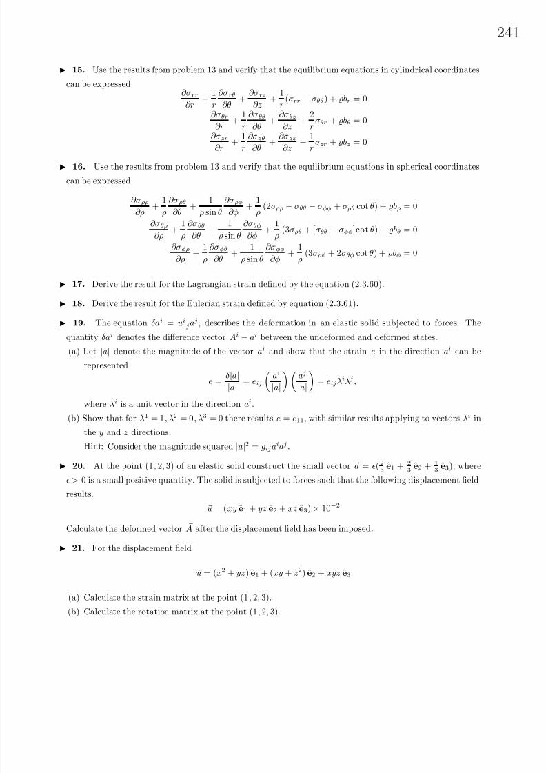
8/6/2019 Introduction to Tensor Calculus Continuum Mechanics - J. Heinbockel
http://slidepdf.com/reader/full/introduction-to-tensor-calculus-continuum-mechanics-j-heinbockel 247/372

8/6/2019 Introduction to Tensor Calculus Continuum Mechanics - J. Heinbockel
http://slidepdf.com/reader/full/introduction-to-tensor-calculus-continuum-mechanics-j-heinbockel 248/372
242
22. Show that for an orthogonal coordinate system the ith component of the convective operator can be
written
[( V · ∇) A]i =
3m=1
V (m)
hm
∂A(i)
∂xm+
3m=1
m=i
A(m)
hmhi
V (i)
∂hi
∂xm− V (m)
∂hm
∂xi
23. Consider a parallelepiped with dimensions ,w,h which has a uniform pressure P applied to eachface. Show that the volume strain can be expressed as
∆V
V =
∆
+
∆w
w+
∆h
h=−3P (1− 2ν )
E .
The quantity k = E/3(1 − 2ν ) is called the bulk modulus of elasticity.
24. Show in Cartesian coordinates the continuity equation is
∂
∂t+
∂ (u)
∂x+
∂ (v)
∂y+
∂ (w)
∂z= 0,
where (u, v, w) are the velocity components.
25. Show in cylindrical coordinates the continuity equation is
∂
∂t+
1
r
∂ (rV r )
∂r+
1
r
∂ (V θ)
∂θ+
∂ (V z)
∂z= 0
where V r, V θ, V z are the velocity components.
26. Show in spherical coordinates the continuity equation is
∂
∂t+
1
ρ2
∂ (ρ2V ρ)
∂ρ+
1
ρ sin θ
∂ (V θ sin θ)
∂θ+
1
ρ sin θ
∂ (V φ)
∂φ= 0
where V ρ, V θ, V φ are the velocity components.
27. (a) Apply a stress σyy to both ends of a square element in a x, y continuum. Illustrate and label
all changes that occur due to this stress. (b) Apply a stress σxx to both ends of a square element in a
x, y continuum. Illustrate and label all changes that occur due to this stress. (c) Use superposition of your
results in parts (a) and (b) and explain each term in the relations
exx =σxx
E − ν
σyy
E and eyy =
σyy
E − ν
σxx
E .
28. Show that the time derivative of the Jacobian J = J
x, y, z
X, Y, Z
satisfies
dJ
dt= J div V where
div V =∂V 1∂x
+∂V 2∂y
+∂V 3∂z
and V 1 =dx
dt, V 2 =
dy
dt, V 3 =
dz
dt.
Hint: Let (x, y, z) = (x1, x2, x3) and (X, Y, Z ) = (X 1, X 2, X 3), then note that
eijk
∂V 1∂X i
∂x2
∂X j
∂x3
∂X k= eijk
∂V 1∂xm
∂xm
∂X i
∂x2
∂X j
∂x3
∂X k= eijk
∂x1
∂X i
∂x2
∂X j
∂x3
∂X k
∂V 1∂x1
, etc.

8/6/2019 Introduction to Tensor Calculus Continuum Mechanics - J. Heinbockel
http://slidepdf.com/reader/full/introduction-to-tensor-calculus-continuum-mechanics-j-heinbockel 249/372
24
§2.4 CONTINUUM MECHANICS (SOLIDS)
In this introduction to continuum mechanics we consider the basic equations describing the physical
effects created by external forces acting upon solids and fluids. In addition to the basic equations that
are applicable to all continua, there are equations which are constructed to take into account material
characteristics. These equations are called constitutive equations. For example, in the study of solids the
constitutive equations for a linear elastic material is a set of relations between stress and strain. In the study
of fluids, the constitutive equations consists of a set of relations between stress and rate of strain. Constitutive
equations are usually constructed from some basic axioms. The resulting equations have unknown material
parameters which can be determined from experimental investigations.
One of the basic axioms, used in the study of elastic solids, is that of material invariance. This ax-
iom requires that certain symmetry conditions of solids are to remain invariant under a set of orthogonal
transformations and translations. This axiom is employed in the next section to simplify the constitutive
equations for elasticity. We begin our study of continuum mechanics by investigating the development of
constitutive equations for linear elastic solids.
Generalized Hooke’s Law
If the continuum material is a linear elastic material, we introduce the generalized Hooke’s law in
Cartesian coordinates
σij = cijklekl, i, j, k, l = 1, 2, 3. (2.4.1)
The Hooke’s law is a statement that the stress is proportional to the gradient of the deformation occurring
in the material. These equations assume a linear relationship exists between the components of the stress
tensor and strain tensor and we say stress is a linear function of strain. Such relations are referred to as a
set of constitutive equations. Constitutive equations serve to describe the material properties of the medium
when it is subjected to external forces.
Constitutive Equations
The equations (2.4.1) are constitutive equations which are applicable for materials exhibiting small
deformations when subjected to external forces. The 81 constants cijkl are called the elastic stiffness of the
material. The above relations can also be expressed in the form
eij = sijklσkl , i, j, k, l = 1, 2, 3 (2.4.2)
where sijkl are constants called the elastic compliance of the material. Since the stress σij and strain eij
have been shown to be tensors we can conclude that both the elastic stiffness cijkl and elastic compliance
sijkl are fourth order tensors. Due to the symmetry of the stress and strain tensors we find that the elasticstiffness and elastic compliance tensor must satisfy the relations
cijkl = cjikl = cijlk = cjilk
sijkl = sjikl = sijlk = sjilk(2.4.3)
and consequently only 36 of the 81 constants are actually independent. If all 36 of the material (crystal)
constants are independent the material is called triclinic and there are no material symmetries.

8/6/2019 Introduction to Tensor Calculus Continuum Mechanics - J. Heinbockel
http://slidepdf.com/reader/full/introduction-to-tensor-calculus-continuum-mechanics-j-heinbockel 250/372
244
Restrictions on Elastic Constants due to Symmetry
The equations (2.4.1) and (2.4.2) can be replaced by an equivalent set of equations which are easier to
analyze. This is accomplished by defining the quantities
e1, e2, e3, e4, e5, e6
σ1, σ2, σ3, σ4, σ5, σ6
where e1 e4 e5
e4 e2 e6e5 e6 e3
=
e11 e12 e13
e21 e22 e23e31 e32 e33
and σ1 σ4 σ5
σ4 σ2 σ6σ5 σ6 σ3
=
σ11 σ12 σ13
σ21 σ22 σ23σ31 σ32 σ33
.
Then the generalized Hooke’s law from the equations (2.4.1) and (2.4.2) can be represented in either of
the formsσi = cijej or ei = sijσj where i, j = 1, . . . , 6 (2.4.4)
where cij are constants related to the elastic stiffness and sij are constants related to the elastic compliance.
These constants satisfy the relation
smicij = δmj where i,m,j = 1, . . . , 6 (2.4.5)
Here
eij =
ei, i = j = 1, 2, 3
e1+i+j, i = j, and i = 1, or, 2
and similarlyσij =
σi, i = j = 1, 2, 3
σ1+i+j , i = j, and i = 1, or, 2.
These relations show that the constants cij are related to the elastic stiffness coefficients c pqrs by the
relationscm1 = cij11
cm2 = cij22
cm3 = cij33
cm4 = 2cij12
cm5 = 2cij13
cm6 = 2cij23
where
m = i, if i = j = 1, 2, or 3
1 + i + j, if i
= j and i = 1or2.
A similar type relation holds for the constants sij and s pqrs. The above relations can be verified by expanding
the equations (2.4.1) and (2.4.2) and comparing like terms with the expanded form of the equation (2.4.4).

8/6/2019 Introduction to Tensor Calculus Continuum Mechanics - J. Heinbockel
http://slidepdf.com/reader/full/introduction-to-tensor-calculus-continuum-mechanics-j-heinbockel 251/372
24
The generalized Hooke’s law can now be expressed in a form where the 36 independent constants can
be examined in more detail under special material symmetries. We will examine the form
e1e2e3
e4e5e6
=
s11 s12 s13 s14 s15 s16s21 s22 s23 s24 s25 s26s31 s32 s33 s34 s35 s36
s41 s42 s43 s44 s45 s46s51 s52 s53 s54 s55 s56s61 s62 s63 s64 s65 s66
σ1σ2σ3
σ4σ5σ6
. (2.4.6)
Alternatively, in the arguments that follow, one can examine the equivalent form
σ1σ2σ3σ4σ5σ6
=
c11 c12 c13 c14 c15 c16c21 c22 c23 c24 c25 c26c31 c32 c33 c34 c35 c36c41 c42 c43 c44 c45 c46c51 c52 c53 c54 c55 c56c61 c62 c63 c64 c65 c66
e1e2e3e4e5e6
.
Material Symmetries
A material (crystal) with one plane of symmetry is called an aelotropic material. If we let the x1-
x2 plane be a plane of symmetry then the equations (2.4.6) must remain invariant under the coordinate
transformation x1
x2x3
=
1 0 0
0 1 00 0 −1
x1
x2x3
(2.4.7)
which represents an inversion of the x3 axis. That is, if the x1-x2 plane is a plane of symmetry we should be
able to replace x3 by −x3 and the equations (2.4.6) should remain unchanged. This is equivalent to saying
that a transformation of the type from equation (2.4.7) changes the Hooke’s law to the form ei = sijσj where
the sij remain unaltered because it is the same material. Employing the transformation equations
x1 = x1, x2 = x2, x3 = −x3 (2.4.8)
we examine the stress and strain transformation equations
σij = σ pq∂x p∂xi
∂xq
∂xj
and eij = e pq∂x p∂xi
∂xq
∂xj
. (2.4.9)
If we expand both of the equations (2.4.9) and substitute in the nonzero derivatives
∂x1
∂x1= 1,
∂x2
∂x2= 1,
∂x3
∂x3= −1, (2.4.10)
we obtain the relations σ11 = σ11
σ22 = σ22
σ33 = σ33
σ21 = σ21
σ31 = −σ31
σ23 = −σ23
e11 = e11
e22 = e22
e33 = e33
e21 = e21
e31 = −e31
e23 = −e23.
(2.4.11)

8/6/2019 Introduction to Tensor Calculus Continuum Mechanics - J. Heinbockel
http://slidepdf.com/reader/full/introduction-to-tensor-calculus-continuum-mechanics-j-heinbockel 252/372
246
We conclude that if the material undergoes a strain, with the x1-x2 plane as a plane of symmetry then
e5 and e6 change sign upon reversal of the x3 axis and e1, e2, e3, e4 remain unchanged. Similarly, we find σ5
and σ6 change sign while σ1, σ2, σ3, σ4 remain unchanged. The equation (2.4.6) then becomes
e1e2e3e4
−e5−e6
=
s11 s12 s13 s14 s15 s16s21 s22 s23 s24 s25 s26s31 s32 s33 s34 s35 s36s41 s42 s43 s44 s45 s46s51 s52 s53 s54 s55 s56s61 s62 s63 s64 s65 s66
σ1σ2σ3σ4
−σ5−σ6
. (2.4.12)
If the stress strain relation for the new orientation of the x3 axis is to have the same form as the
old orientation, then the equations (2.4.6) and (2.4.12) must give the same results. Comparison of these
equations we find thats15 = s16 = 0
s25 = s26 = 0
s35 = s36 = 0
s45 = s46 = 0
s51 = s52 = s53 = s54 = 0
s61 = s62 = s63 = s64 = 0.
(2.4.13)
In summary, from an examination of the equations (2.4.6) and (2.4.12) we find that for an aelotropic
material (crystal), with one plane of symmetry, the 36 constants sij reduce to 20 constants and the generalized
Hooke’s law (constitutive equation) has the form
e1e2e3e4e5e6
=
s11 s12 s13 s14 0 0s21 s22 s23 s24 0 0s31 s32 s33 s34 0 0s41 s42 s43 s44 0 0
0 0 0 0 s55 s560 0 0 0 s65 s66
σ1σ2σ3σ4σ5σ6
. (2.4.14)
Alternatively, the Hooke’s law can be represented in the form
σ1σ2σ3σ4σ5σ6
=
c11 c12 c13 c14 0 0c21 c22 c23 c24 0 0c31 c32 c33 c34 0 0c41 c42 c43 c44 0 00 0 0 0 c55 c560 0 0 0 c65 c66
e1e2e3e4e5e6
.

8/6/2019 Introduction to Tensor Calculus Continuum Mechanics - J. Heinbockel
http://slidepdf.com/reader/full/introduction-to-tensor-calculus-continuum-mechanics-j-heinbockel 253/372
24
Additional Symmetries
If the material (crystal) is such that there is an additional plane of symmetry, say the x2-x3 plane, then
reversal of the x1 axis should leave the equations (2.4.14) unaltered. If there are two planes of symmetry
then there will automatically be a third plane of symmetry. Such a material (crystal) is called orthotropic.
Introducing the additional transformation
x1 = −x1, x2 = x2, x3 = x3
which represents the reversal of the x1 axes, the expanded form of equations (2.4.9) are used to calculate the
effect of such a transformation upon the stress and strain tensor. We find σ1, σ2, σ3, σ6, e1, e2, e3, e6 remain
unchanged while σ4, σ5, e4, e5 change sign. The equation (2.4.14) then becomes
e1e2e3
−e4
−e5e6
=
s11 s12 s13 s14 0 0s21 s22 s23 s24 0 0s31 s32 s33 s34 0 0s41 s42 s43 s44 0 0
0 0 0 0 s55 s560 0 0 0 s65 s66
σ1σ2σ3
−σ4
−σ5σ6
. (2.4.15)
Note that if the constitutive equations (2.4.14) and (2.4.15) are to produce the same results upon reversal
of the x1 axes, then we require that the following coefficients be equated to zero:
s14 = s24 = s34 = 0
s41 = s42 = s43 = 0
s56 = s65 = 0.
This then produces the constitutive equation
e1e2e3e4e5e6
=
s11 s12 s13 0 0 0s21 s22 s23 0 0 0s31 s32 s33 0 0 0
0 0 0 s44 0 00 0 0 0 s55 00 0 0 0 0 s66
σ1σ2σ3σ4σ5σ6
(2.4.16)
or its equivalent form
σ1σ2σ3σ4σ5
σ6
=
c11 c12 c13 0 0 0c21 c22 c23 0 0 0c31 c32 c33 0 0 00 0 0 c44 0 00 0 0 0 c55 0
0 0 0 0 0 c66
e1e2e3e4e5
e6
and the original 36 constants have been reduced to 12 constants. This is the constitutive equation for
orthotropic material (crystals).

8/6/2019 Introduction to Tensor Calculus Continuum Mechanics - J. Heinbockel
http://slidepdf.com/reader/full/introduction-to-tensor-calculus-continuum-mechanics-j-heinbockel 254/372
248
Axis of Symmetry
If in addition to three planes of symmetry there is an axis of symmetry then the material (crystal) is
termed hexagonal. Assume that the x1 axis is an axis of symmetry and consider the effect of the transfor-
mation
x
1
= x
1
, x
2
= x
3
x
3
= −x
2
upon the constitutive equations. It is left as an exercise to verify that the constitutive equations reduce to
the form where there are 7 independent constants having either of the forms
e1e2e3e4e5e6
=
s11 s12 s12 0 0 0s21 s22 s23 0 0 0s21 s23 s22 0 0 0
0 0 0 s44 0 00 0 0 0 s44 00 0 0 0 0 s66
σ1σ2σ3σ4σ5σ6
or
σ1
σ2σ3σ4σ5σ6
=
c11 c12 c12 0 0 0
c21 c22 c23 0 0 0c21 c23 c22 0 0 00 0 0 c44 0 00 0 0 0 c44 00 0 0 0 0 c66
e1
e2e3e4e5e6
.
Finally, if the material is completely symmetric, the x2 axis is also an axis of symmetry and we can
consider the effect of the transformation
x1 = −x3, x2 = x2, x3 = x1
upon the constitutive equations. It can be verified that these transformations reduce the Hooke’s law
constitutive equation to the form
e1e2e3e4e5e6
=
s11 s12 s12 0 0 0s12 s11 s12 0 0 0s12 s12 s11 0 0 0
0 0 0 s44 0 00 0 0 0 s44 00 0 0 0 0 s44
σ1σ2σ3σ4σ5σ6
. (2.4.17)
Materials (crystals) with atomic arrangements that exhibit the above symmetries are called isotropic
materials. An equivalent form of (2.4.17) is the relation
σ1σ2σ3σ4σ5σ6
=
c11 c12 c12 0 0 0c12 c11 c12 0 0 0
c12 c12 c11 0 0 00 0 0 c44 0 00 0 0 0 c44 00 0 0 0 0 c44
e1e2e3e4e5e6
.
The figure 2.4-1 lists values for the elastic stiffness associated with some metals which are isotropic 1
1Additional constants are given in “International Tables of Selected Constants”, Metals: Thermal and
Mechanical Data, Vol. 16, Edited by S. Allard, Pergamon Press, 1969.
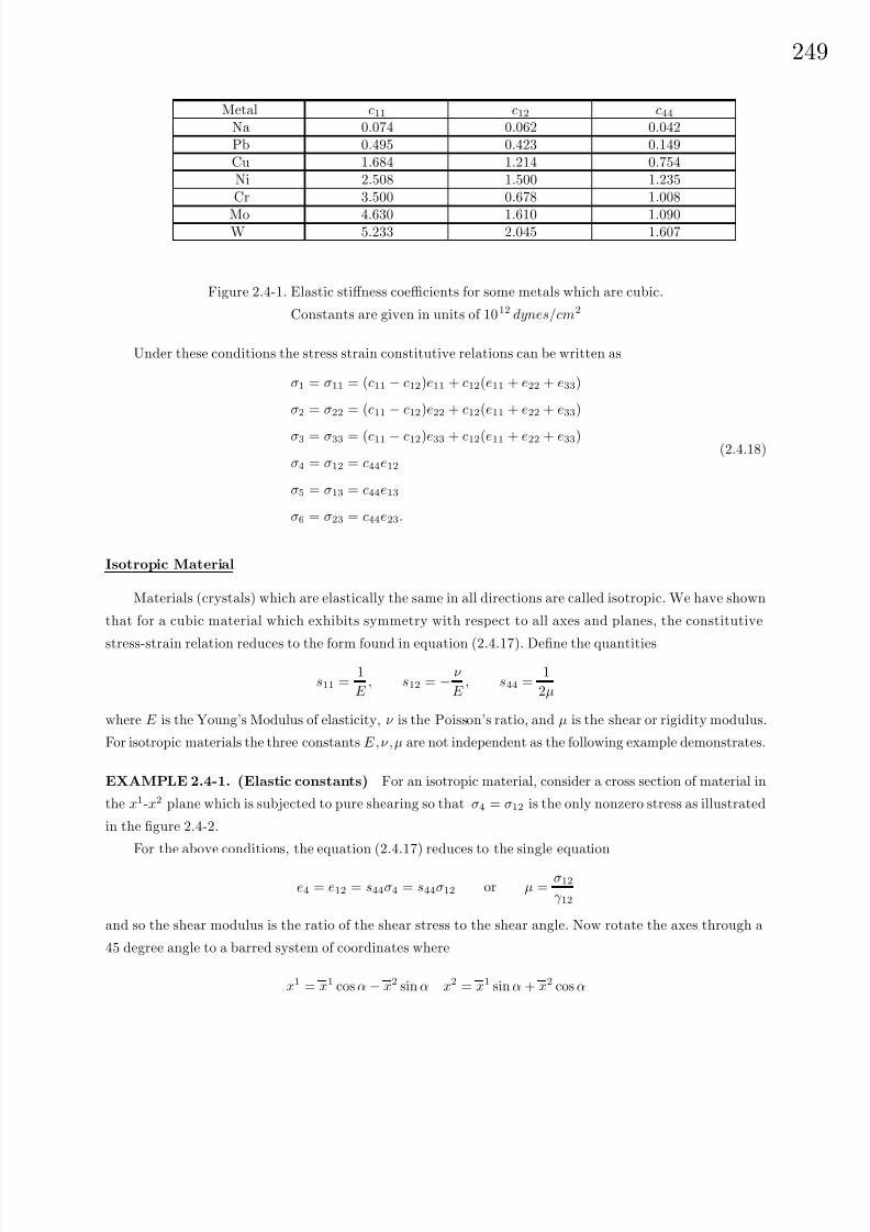
8/6/2019 Introduction to Tensor Calculus Continuum Mechanics - J. Heinbockel
http://slidepdf.com/reader/full/introduction-to-tensor-calculus-continuum-mechanics-j-heinbockel 255/372
24
Metal c11 c12 c44Na 0.074 0.062 0.042Pb 0.495 0.423 0.149Cu 1.684 1.214 0.754Ni 2.508 1.500 1.235Cr 3.500 0.678 1.008
Mo 4.630 1.610 1.090W 5.233 2.045 1.607
Figure 2.4-1. Elastic stiffness coefficients for some metals which are cubic.
Constants are given in units of 1012 dynes/cm2
Under these conditions the stress strain constitutive relations can be written as
σ1 = σ11 = (c11 − c12)e11 + c12(e11 + e22 + e33)
σ2 = σ22 = (c11 − c12)e22 + c12(e11 + e22 + e33)
σ3 = σ33 = (c11 − c12)e33 + c12(e11 + e22 + e33)
σ4 = σ12 = c44e12
σ5 = σ13 = c44e13
σ6 = σ23 = c44e23.
(2.4.18)
Isotropic Material
Materials (crystals) which are elastically the same in all directions are called isotropic. We have shown
that for a cubic material which exhibits symmetry with respect to all axes and planes, the constitutive
stress-strain relation reduces to the form found in equation (2.4.17). Define the quantities
s11 =1
E , s12 = − ν
E , s44 =
1
2µ
where E is the Young’s Modulus of elasticity, ν is the Poisson’s ratio, and µ is the shear or rigidity modulus.
For isotropic materials the three constants E, ν , µ are not independent as the following example demonstrates.
EXAMPLE 2.4-1. (Elastic constants) For an isotropic material, consider a cross section of material in
the x1-x2 plane which is subjected to pure shearing so that σ4 = σ12 is the only nonzero stress as illustrated
in the figure 2.4-2.
For the above conditions, the equation (2.4.17) reduces to the single equation
e4 = e12 = s44σ4 = s44σ12 or µ =σ12γ 12
and so the shear modulus is the ratio of the shear stress to the shear angle. Now rotate the axes through a
45 degree angle to a barred system of coordinates where
x1 = x1 cos α − x2 sin α x2 = x1 sin α + x2 cos α

8/6/2019 Introduction to Tensor Calculus Continuum Mechanics - J. Heinbockel
http://slidepdf.com/reader/full/introduction-to-tensor-calculus-continuum-mechanics-j-heinbockel 256/372

8/6/2019 Introduction to Tensor Calculus Continuum Mechanics - J. Heinbockel
http://slidepdf.com/reader/full/introduction-to-tensor-calculus-continuum-mechanics-j-heinbockel 257/372
25
The previous discussion has shown that for an isotropic material the generalized Hooke’s law (constitu-
tive equations) have the form
e11 =1
E [σ11 − ν (σ22 + σ33)]
e22 =
1
E [σ22 − ν (σ33 + σ11)]
e33 =1
E [σ33 − ν (σ11 + σ22)]
e21 = e12 =1 + ν
E σ12
e32 = e23 =1 + ν
E σ23
e31 = e13 =1 + ν
E σ13
, (2.4.20)
where equation (2.4.19) holds. These equations can be expressed in the indicial notation and have the form
eij =1 + ν
E
σij
−
ν
E
σkkδij , (2.4.21)
where σkk = σ11 + σ22 + σ33 is a stress invariant and δij is the Kronecker delta. We can solve for the stress
in terms of the strain by performing a contraction on i and j in equation (2.4.21). This gives the dilatation
eii =1 + ν
E σii − 3ν
E σkk =
1 − 2ν
E σkk .
Note that from the result in equation (2.4.21) we are now able to solve for the stress in terms of the strain.
We find
eij =1 + ν
E σij − ν
1
−2ν
ekkδij
E 1 + ν
eij = σij − νE (1 + ν )(1 − 2ν )
ekkδij
or σij =E
1 + ν eij +
νE
(1 + ν )(1 − 2ν )ekkδij .
(2.4.22)
The tensor equation (2.4.22) represents the six scalar equations
σ11 =E
(1 + ν )(1 − 2ν )[(1 − ν )e11 + ν (e22 + e33)]
σ22 =E
(1 + ν )(1 − 2ν )[(1 − ν )e22 + ν (e33 + e11)]
σ33 =E
(1 + ν )(1 − 2ν )
[(1
−ν )e33 + ν (e22 + e11)]
σ12 =E
1 + ν e12
σ13 =E
1 + ν e13
σ23 =E
1 + ν
e23.

8/6/2019 Introduction to Tensor Calculus Continuum Mechanics - J. Heinbockel
http://slidepdf.com/reader/full/introduction-to-tensor-calculus-continuum-mechanics-j-heinbockel 258/372
252
Alternative Approach to Constitutive Equations
The constitutive equation defined by Hooke’s generalized law for isotropic materials can be approached
from another point of view. Consider the generalized Hooke’s law
σij = cijklekl, i, j, k, l = 1, 2, 3.
If we transform to a barred system of coordinates, we will have the new Hooke’s law
σij = cijklekl, i, j, k, l = 1, 2, 3.
For an isotropic material we require that
cijkl = cijkl.
Tensors whose components are the same in all coordinate systems are called isotropic tensors. We have
previously shown in Exercise 1.3, problem 18, that
c pqrs = λδ pqδrs + µ(δ prδqs + δ psδqr) + κ(δ prδqs − δ psδqr)
is an isotropic tensor when we consider affine type transformations. If we further require the symmetry
conditions found in equations (2.4.3) be satisfied, we find that κ = 0 and consequently the generalized
Hooke’s law must have the form
σ pq = c pqrsers = [λδ pqδrs + µ(δ prδqs + δ psδqr)] ers
σ pq = λδ pqerr + µ(e pq + eqp)
or σ pq = 2µe pq + λerrδ pq,
(2.4.23)
where err
= e11
+ e22
+ e33
= Θ is the dilatation. The constants λ and µ are called Lame’s constants.
Comparing the equation (2.4.22) with equation (2.4.23) we find that the constants λ and µ satisfy the
relations
µ =E
2(1 + ν )λ =
νE
(1 + ν )(1 − 2ν ). (2.4.24)
In addition to the constants E, ν , µ , λ, it is sometimes convenient to introduce the constant k, called the bulk
modulus of elasticity, (Exercise 2.3, problem 23), defined by
k =E
3(1 − 2ν ). (2.4.25)
The stress-strain constitutive equation (2.4.23) was derived using Cartesian tensors. To generalize the
equation (2.4.23) we consider a transformation from a Cartesian coordinate system yi, i = 1, 2, 3 to a general
coordinate system xi, i = 1, 2, 3. We employ the relations
gij =∂ym
∂xi
∂ym
∂xj, gij =
∂xi
∂ym
∂xj
∂ym
and
σmn = σij
∂y i
∂xm
∂yj
∂xn , emn = eij∂y i
∂xm
∂yj
∂xn , or erq = eij∂xi
∂yr
∂xj
∂yq
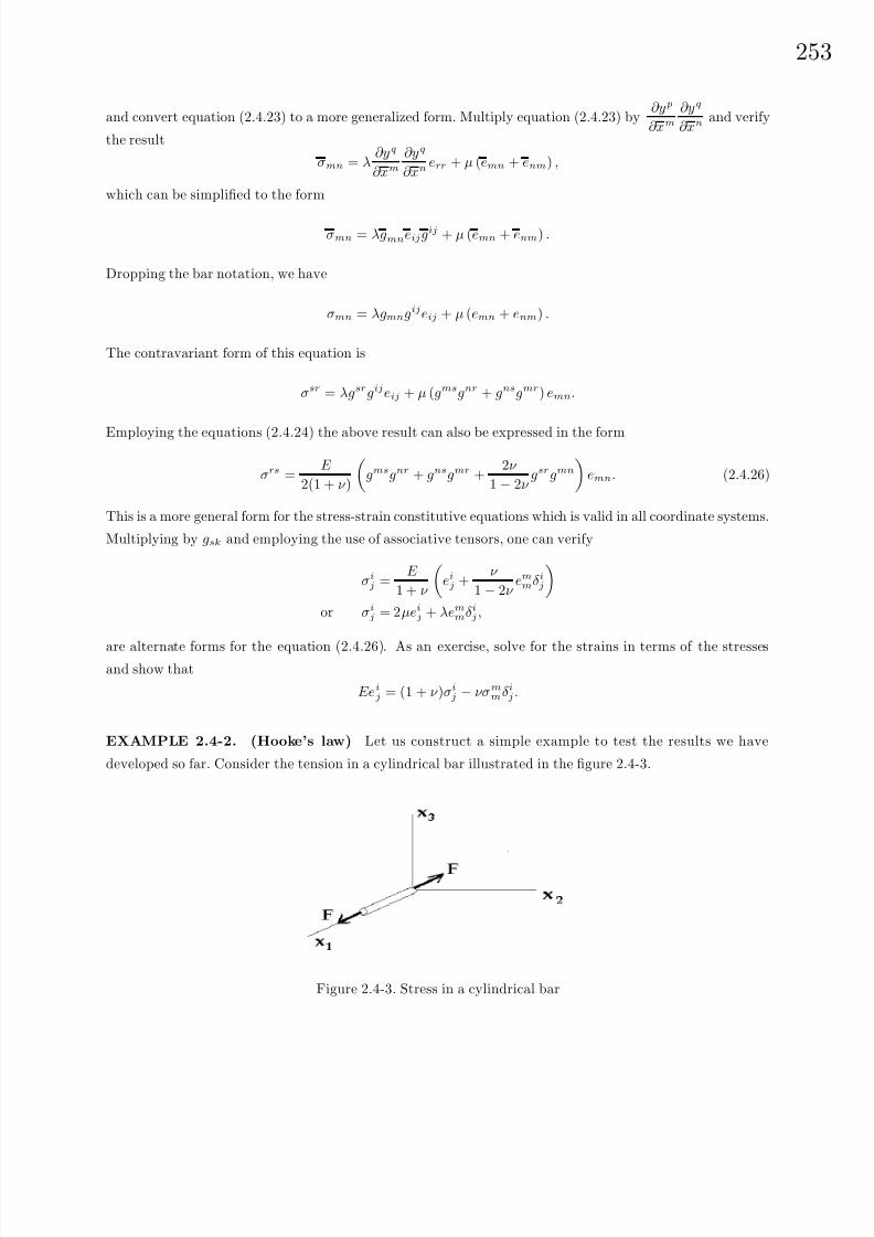
8/6/2019 Introduction to Tensor Calculus Continuum Mechanics - J. Heinbockel
http://slidepdf.com/reader/full/introduction-to-tensor-calculus-continuum-mechanics-j-heinbockel 259/372

8/6/2019 Introduction to Tensor Calculus Continuum Mechanics - J. Heinbockel
http://slidepdf.com/reader/full/introduction-to-tensor-calculus-continuum-mechanics-j-heinbockel 260/372
254
Assume that
σij =
F
A0 0
0 0 00 0 0
where F is the constant applied force and A is the cross sectional area of the cylinder. Consequently, the
generalized Hooke’s law (2.4.21) produces the nonzero strains
e11 =1 + ν
E σ11 − ν
E (σ11 + σ22 + σ33) =
σ11E
e22 =−ν
E σ11
e33 =−ν
E σ11
From these equations we obtain:
The first part of Hooke’s law
σ11 = Ee11 orF
A= Ee11.
The second part of Hooke’s law
lateral contraction
longitudinal extension=
−e22e11
=−e33e11
= ν = Poisson’s ratio.
This example demonstrates that the generalized Hooke’s law for homogeneous and isotropic materials
reduces to our previous one dimensional result given in (2.3.1) and (2.3.2).
Basic Equations of Elasticity
Assuming the density is constant, the basic equations of elasticity reduce to the equations representing
conservation of linear momentum and angular momentum together with the strain-displacement relations
and constitutive equations. In these equations the body forces are assumed known. These basic equations
produce 15 equations in 15 unknowns and are a formidable set of equations to solve. Methods for solving
these simultaneous equations are: 1) Express the linear momentum equations in terms of the displacements
ui and obtain a system of partial differential equations. Solve the system of partial differential equations
for the displacements ui and then calculate the corresponding strains. The strains can be used to calculate
the stresses from the constitutive equations. 2) Solve for the stresses and from the stresses calculate the
strains and from the strains calculate the displacements. This converse problem requires some additional
considerations which will be addressed shortly.
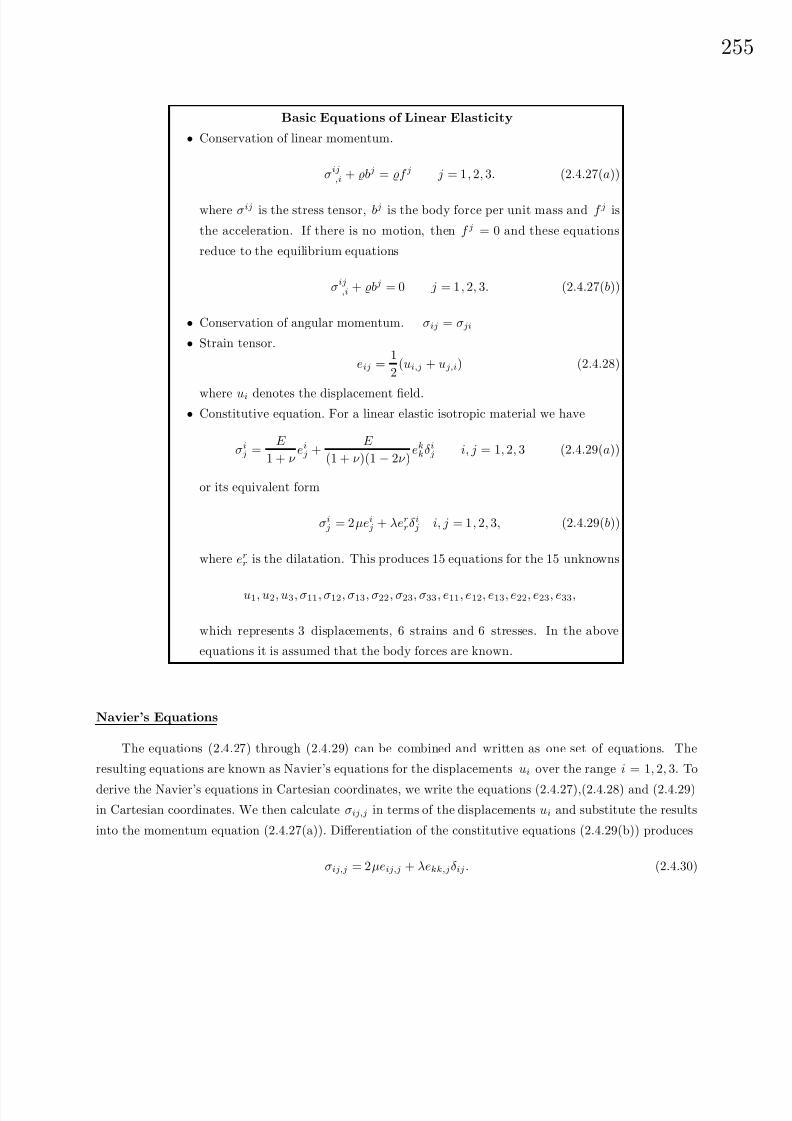
8/6/2019 Introduction to Tensor Calculus Continuum Mechanics - J. Heinbockel
http://slidepdf.com/reader/full/introduction-to-tensor-calculus-continuum-mechanics-j-heinbockel 261/372
25
Basic Equations of Linear Elasticity
• Conservation of linear momentum.
σij,i + bj = f j j = 1, 2, 3. (2.4.27(a))
where σij is the stress tensor, bj is the body force per unit mass and f j is
the acceleration. If there is no motion, then f j = 0 and these equations
reduce to the equilibrium equations
σij,i + bj = 0 j = 1, 2, 3. (2.4.27(b))
• Conservation of angular momentum. σij = σji
• Strain tensor.
eij =1
2(ui,j + uj,i) (2.4.28)
where ui denotes the displacement field.• Constitutive equation. For a linear elastic isotropic material we have
σij =
E
1 + ν eij +
E
(1 + ν )(1 − 2ν )ekkδij i, j = 1, 2, 3 (2.4.29(a))
or its equivalent form
σij = 2µeij + λerrδij i, j = 1, 2, 3, (2.4.29(b))
where err is the dilatation. This produces 15 equations for the 15 unknowns
u1, u2, u3, σ11, σ12, σ13, σ22, σ23, σ33, e11, e12, e13, e22, e23, e33,
which represents 3 displacements, 6 strains and 6 stresses. In the above
equations it is assumed that the body forces are known.
Navier’s Equations
The equations (2.4.27) through (2.4.29) can be combined and written as one set of equations. The
resulting equations are known as Navier’s equations for the displacements ui over the range i = 1, 2, 3. To
derive the Navier’s equations in Cartesian coordinates, we write the equations (2.4.27),(2.4.28) and (2.4.29)
in Cartesian coordinates. We then calculate σij,j in terms of the displacements ui and substitute the results
into the momentum equation (2.4.27(a)). Differentiation of the constitutive equations (2.4.29(b)) produces
σij,j = 2µeij,j + λekk,jδij. (2.4.30)

8/6/2019 Introduction to Tensor Calculus Continuum Mechanics - J. Heinbockel
http://slidepdf.com/reader/full/introduction-to-tensor-calculus-continuum-mechanics-j-heinbockel 262/372
256
A contraction of the strain produces the dilatation
err =1
2(ur,r + ur,r) = ur,r (2.4.31)
From the dilatation we calculate the covariant derivative
ekk,j = uk,kj . (2.4.32)
Employing the strain relation from equation (2.4.28), we calculate the covariant derivative
eij,j =1
2(ui,jj + uj,ij). (2.4.33)
These results allow us to express the covariant derivative of the stress in terms of the displacement field. We
findσij,j = µ [ui,jj + uj,ij ] + λδijuk,kj
or σij,j = (λ + µ)uk,ki + µui,jj .(2.4.34)
Substituting equation (2.4.34) into the linear momentum equation produces the Navier equations:
(λ + µ)uk,ki + µui,jj + bi = f i, i = 1, 2, 3. (2.4.35)
In vector form these equations can be expressed
(λ + µ)∇ (∇ · u) + µ∇2u + b = f, (2.4.36)
where u is the displacement vector, b is the body force per unit mass and f is the acceleration. In Cartesian
coordinates these equations have the form:
(λ + µ)
∂ 2u1
∂x1∂xi
+ ∂ 2u2
∂x2∂xi
+ ∂ 2u3∂x3∂xi
+ µ∇2ui + bi = ∂ 2ui
∂t2,
for i = 1, 2, 3, where
∇2ui =∂ 2ui
∂x12
+∂ 2ui
∂x22
+∂ 2ui
∂x32
.
The Navier equations must be satisfied by a set of functions ui = ui(x1, x2, x3) which represent the
displacement at each point inside some prescribed region R. Knowing the displacement field we can calculate
the strain field directly using the equation (2.4.28). Knowledge of the strain field enables us to construct the
corresponding stress field from the constitutive equations.
In the absence of body forces, such as gravity, the solution to equation (2.4.36) can be represented
in the form u = u (1) + u (2), where u (1) satisfies div u (1) = ∇ · u (1) = 0 and the vector u (2) satisfies
curl u (2) = ∇ × u (2) = 0. The vector field u (1) is called a solenoidal field, while the vector field u (2) is
called an irrotational field. Substituting u into the equation (2.4.36) and setting b = 0, we find in Cartesian
coordinates that
∂ 2u (1)
∂t2+
∂ 2u (2)
∂t2
= (λ + µ)∇
∇ · u (2)
+ µ∇2u (1) + µ∇2u (2). (2.4.37)

8/6/2019 Introduction to Tensor Calculus Continuum Mechanics - J. Heinbockel
http://slidepdf.com/reader/full/introduction-to-tensor-calculus-continuum-mechanics-j-heinbockel 263/372
25
The vector field u (1) can be eliminated from equation (2.4.37) by taking the divergence of both sides of the
equation. This produces
∂ 2∇ · u (2)
∂t2= (λ + µ)∇2(∇ · u (2)) + µ∇ · ∇2u (2).
The displacement field is assumed to be continuous and so we can interchange the order of the operators ∇2
and ∇ and write
∇ ·
∂ 2u (2)
∂t2− (λ + 2µ)∇2u (2)
= 0.
This last equation implies that
∂ 2u (2)
∂t2= (λ + 2µ)∇2u(2)
and consequently, u (2) is a vector wave which moves with the speed
(λ + 2µ)/. Similarly, when the vector
field u (2) is eliminated from the equation (2.4.37), by taking the curl of both sides, we find the vector u (1)
also satisfies a wave equation having the form
∂ 2u (1)
∂t2= µ∇2u (1).
This later wave moves with the speed
µ/. The vector u (2) is a compressive wave, while the wave u (1) is
a shearing wave.
The exercises 30 through 38 enable us to write the Navier’s equations in Cartesian, cylindrical or
spherical coordinates. In particular, we have for cartesian coordinates
(λ + µ)(∂ 2u
∂x2+
∂ 2v
∂x∂y+
∂ 2w
∂x∂z) + µ(
∂ 2u
∂x2+
∂ 2u
∂y2+
∂ 2u
∂z2) + bx =
∂ 2u
∂t2
(λ + µ)(∂ 2u
∂x∂y+
∂ 2v
∂y2
+∂ 2w
∂y∂z) + µ(
∂ 2v
∂x2
+∂ 2v
∂y2
+∂ 2v
∂z2) + by =
∂ 2v
∂t2
(λ + µ)(∂ 2u
∂x∂z+
∂ 2v
∂y∂z+
∂ 2w
∂z2) + µ(
∂ 2w
∂x2+
∂ 2w
∂y2+
∂ 2w
∂z2) + bz =
∂ 2w
∂t2
and in cylindrical coordinates
(λ + µ)∂
∂r
1
r
∂
∂r(rur) +
1
r
∂uθ
∂θ+
∂uz
∂z
+
µ(∂ 2ur
∂r2+
1
r
∂ur
∂r+
1
r2∂ 2ur
∂θ2+
∂ 2ur
∂z2− ur
r2− 2
r2∂uθ
∂θ) + br =
∂ 2ur
∂t2
(λ + µ)1
r
∂
∂θ 1
r
∂
∂r(rur) +
1
r
∂uθ
∂θ+
∂uz
∂z +
µ(∂ 2uθ
∂r2+
1
r
∂uθ
∂r+
1
r2∂ 2uθ
∂θ2+
∂ 2uθ
∂z2+
2
r2∂ur
∂θ− uθ
r2) + bθ =
∂ 2uθ
∂t2
(λ + µ)∂
∂z
1
r
∂
∂r(rur) +
1
r
∂uθ
∂θ+
∂uz
∂z
+
µ(∂ 2uz
∂r2+
1
r
∂uz
∂r+
1
r2∂ 2uz
∂θ2+
∂ 2uz
∂z2) + bz =
∂ 2uz
∂t2
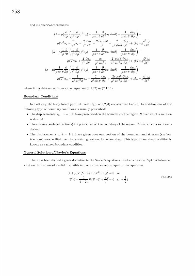
8/6/2019 Introduction to Tensor Calculus Continuum Mechanics - J. Heinbockel
http://slidepdf.com/reader/full/introduction-to-tensor-calculus-continuum-mechanics-j-heinbockel 264/372
258
and in spherical coordinates
(λ + µ)∂
∂ρ
1
ρ2∂
∂ρ(ρ2uρ) +
1
ρ sin θ
∂
∂θ(uθ sin θ) +
1
ρ sin θ
∂uφ
∂φ
+
µ(∇2uρ − 2
ρ2uρ − 2
ρ2∂uθ
∂θ− 2uθ cot θ
ρ2− 2
ρ2 sin θ
∂uφ
∂φ) + bρ =
∂ 2uρ
∂t2
(λ + µ)1
ρ
∂
∂θ
1
ρ2∂
∂ρ(ρ2uρ) +
1
ρ sin θ
∂
∂θ(uθ sin θ) +
1
ρ sin θ
∂uφ
∂φ
+
µ(∇2uθ +2
ρ2∂uρ
∂θ− uθ
ρ2 sin2 θ− 2
ρ2cos θ
sin2 θ
∂uφ
∂φ) + bθ =
∂ 2uθ
∂t2
(λ + µ)1
ρ sin θ
∂
∂φ
1
ρ2∂
∂ρ(ρ2uρ) +
1
ρ sin θ
∂
∂θ(uθ sin θ) +
1
ρ sin θ
∂uφ
∂φ
+
µ(∇2uφ − 1
ρ2 sin2 θuφ +
2
ρ2 sin θ
∂uρ
∂φ+
2cos θ
ρ2 sin2 θ
∂uθ
∂φ) + bφ =
∂ 2uφ
∂t2
where ∇2 is determined from either equation (2.1.12) or (2.1.13).
Boundary Conditions
In elasticity the body forces per unit mass (bi, i = 1, 2, 3) are assumed known. In addition one of the
following type of boundary conditions is usually prescribed:
• The displacements ui, i = 1, 2, 3 are prescribed on the boundary of the region R over which a solution
is desired.
• The stresses (surface tractions) are prescribed on the boundary of the region R over which a solution is
desired.
• The displacements ui, i = 1, 2, 3 are given over one portion of the boundary and stresses (surface
tractions) are specified over the remaining portion of the boundary. This type of boundary condition is
known as a mixed boundary condition.
General Solution of Navier’s Equations
There has been derived a general solution to the Navier’s equations. It is known as the Papkovich-Neuber
solution. In the case of a solid in equilibrium one must solve the equilibrium equations
(λ + µ)∇ (∇ · u) + µ∇2u + b = 0 or
∇2 u +1
1 − 2ν ∇(∇ · u) +
µ b = 0 (ν = 1
2)
(2.4.38)

8/6/2019 Introduction to Tensor Calculus Continuum Mechanics - J. Heinbockel
http://slidepdf.com/reader/full/introduction-to-tensor-calculus-continuum-mechanics-j-heinbockel 265/372
25
THEOREM A general elastostatic solution of the equation (2.4.38) in terms of harmonic potentials φ, ψ
is
u = grad (φ + r · ψ) − 4(1 − ν ) ψ (2.4.39)
where φ and ψ are continuous solutions of the equations
∇2φ = −r · b4µ(1 − ν )
and ∇2 ψ = b4µ(1 − ν )
(2.4.40)
with r = x e1 + y e2 + z e3 a position vector to a general point (x, y, z) within the continuum.
Proof: First we write equation (2.4.38) in the tensor form
ui,kk +1
1 − 2ν (uj,j) ,i +
µbi = 0 (2.4.41)
Now our problem is to show that equation (2.4.39), in tensor form,
ui = φ,i + (xjψj),i − 4(1 − ν )ψi (2.4.42)
is a solution of equation (2.4.41). Toward this purpose, we differentiate equation (2.4.42)
ui,k = φ,ik + (xjψj),ik − 4(1 − ν )ψi,k (2.4.43)
and then contract on i and k giving
ui,i = φ,ii + (xjψj),ii − 4(1 − ν )ψi,i. (2.4.44)
Employing the identity (xjψj),ii = 2ψi,i + xiψi,kk the equation (2.4.44) becomes
ui,i = φ,ii + 2ψi,i + xiψi,kk − 4(1 − ν )ψi,i. (2.4.45)
By differentiating equation (2.4.43) we establish that
ui,kk = φ,ikk + (xjψj),ikk − 4(1 − ν )ψi,kk
= (φ,kk),i + ((xjψj),kk),i
− 4(1 − ν )ψi,kk
= [φ,kk + 2ψj,j + xjψj,kk],i
− 4(1 − ν )ψi,kk .
(2.4.46)
We use the hypothesis
φ,kk =−xjF j
4µ(1 − ν )and ψj,kk =
F j4µ(1 − ν )
,
and simplify the equation (2.4.46) to the form
ui,kk = 2ψj,ji − 4(1 − ν )ψi,kk . (2.4.47)
Also by differentiating (2.4.45) one can establish that
uj,ji = (φ,jj ),i + 2ψj,ji + (xjψj,kk),i − 4(1 − ν )ψj,ji
=
−xjF j4µ(1 − ν )
,i
+ 2ψj,ji +
xjF j
4µ(1 − ν )
,i
− 4(1 − ν )ψj,ji
= −2(1 − 2ν )ψj,ji.
(2.4.48)

8/6/2019 Introduction to Tensor Calculus Continuum Mechanics - J. Heinbockel
http://slidepdf.com/reader/full/introduction-to-tensor-calculus-continuum-mechanics-j-heinbockel 266/372
260
Finally, from the equations (2.4.47) and (2.4.48) we obtain the desired result that
ui,kk +1
1 − 2ν uj,ji +
F iµ
= 0.
Consequently, the equation (2.4.39) is a solution of equation (2.4.38).
As a special case of the above theorem, note that when the body forces are zero, the equations (2.4.40)become
∇2φ = 0 and ∇2 ψ = 0.
In this case, we find that equation (2.4.39) is a solution of equation (2.4.38) provided φ and each component of
ψ are harmonic functions. The Papkovich-Neuber potentials are used together with complex variable theory
to solve various two-dimensional elastostatic problems of elasticity. Note also that the Papkovich-Neuber
potentials are not unique as different combinations of φ and ψ can produce the same value for u.
Compatibility Equations
If we know or can derive the displacement field ui, i = 1, 2, 3 we can then calculate the components of the strain tensor
eij =1
2(ui,j + uj,i). (2.4.49)
Knowing the strain components, the stress is found using the constitutive relations.
Consider the converse problem where the strain tensor is given or implied due to the assigned stress
field and we are asked to determine the displacement field ui, i = 1, 2, 3. Is this a realistic request? Is it even
possible to solve for three displacements given six strain components? It turns out that certain mathematical
restrictions must be placed upon the strain components in order that the inverse problem have a solution.
These mathematical restrictions are known as compatibility equations. That is, we cannot arbitrarily assign
six strain components eij and expect to find a displacement field ui, i = 1, 2, 3 with three components which
satisfies the strain relation as given in equation (2.4.49).
EXAMPLE 2.4-3. Suppose we are given the two partial differential equations,
∂u
∂x= x + y and
∂u
∂y= x3.
Can we solve for u = u(x, y)? The answer to this question is “no”, because the given equations are inconsis-
tent. The inconsistency is illustrated if we calculate the mixed second derivatives from each equation. We
find from the first equation that∂ 2u
∂x∂y= 1 and from the second equation we calculate
∂ 2u
∂y∂x= 3x2. These
mixed second partial derivatives are unequal for all x different from√
3/3. In general, if we have two first
order partial differential equations∂u∂x
= f (x, y) and∂u∂y
= g(x, y), then for consistency (integrability of
the equations) we require that the mixed partial derivatives
∂ 2u
∂x∂y=
∂f
∂y=
∂ 2u
∂y∂x=
∂g
∂x
be equal to one another for all x and y values over the domain for which the solution is desired. This is an
example of a compatibility equation.
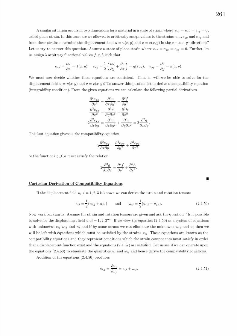
8/6/2019 Introduction to Tensor Calculus Continuum Mechanics - J. Heinbockel
http://slidepdf.com/reader/full/introduction-to-tensor-calculus-continuum-mechanics-j-heinbockel 267/372
26
A similar situation occurs in two dimensions for a material in a state of strain where ezz = ezx = ezy = 0,
called plane strain. In this case, are we allowed to arbitrarily assign values to the strains exx, eyy and exy and
from these strains determine the displacement field u = u(x, y) and v = v(x, y) in the x− and y−directions?
Let us try to answer this question. Assume a state of plane strain where ezz = ezx = ezy = 0. Further, let
us assign 3 arbitrary functional values f , g , h such that
exx =∂u
∂x= f (x, y), exy =
1
2
∂u
∂y+
∂v
∂x
= g(x, y), eyy =
∂v
∂y= h(x, y).
We must now decide whether these equations are consistent. That is, will we be able to solve for the
displacement field u = u(x, y) and v = v(x, y)? To answer this question, let us derive a compatibility equation
(integrability condition). From the given equations we can calculate the following partial derivatives
∂ 2exx∂y2
=∂ 3u
∂x∂y2=
∂ 2f
∂y2
∂ 2eyy∂x2
=∂ 3v
∂y∂x2=
∂ 2h
∂x2
2∂ 2exy∂x∂y
=∂ 3u
∂x∂y2+
∂ 3v
∂y∂x2= 2
∂ 2g
∂x∂y.
This last equation gives us the compatibility equation
2∂ 2exy∂x∂y
=∂ 2exx
∂y2+
∂ 2eyy∂x2
or the functions g , f , h must satisfy the relation
2∂ 2g
∂x∂y=
∂ 2f
∂y2+
∂ 2h
∂x2.
Cartesian Derivation of Compatibility Equations
If the displacement field ui, i = 1, 2, 3 is known we can derive the strain and rotation tensors
eij =1
2(ui,j + uj,i) and ωij =
1
2(ui,j − uj,i). (2.4.50)
Now work backwards. Assume the strain and rotation tensors are given and ask the question, “Is it possible
to solve for the displacement field ui, i = 1, 2, 3?” If we view the equation (2.4.50) as a system of equations
with unknowns eij , ωij and ui and if by some means we can eliminate the unknowns ωij and ui then we
will be left with equations which must be satisfied by the strains eij . These equations are known as the
compatibility equations and they represent conditions which the strain components must satisfy in order
that a displacement function exist and the equations (2.4.37) are satisfied. Let us see if we can operate upon
the equations (2.4.50) to eliminate the quantities ui and ωij and hence derive the compatibility equations.
Addition of the equations (2.4.50) produces
ui,j =∂ui
∂xj
= eij + ωij. (2.4.51)

8/6/2019 Introduction to Tensor Calculus Continuum Mechanics - J. Heinbockel
http://slidepdf.com/reader/full/introduction-to-tensor-calculus-continuum-mechanics-j-heinbockel 268/372
262
Differentiate this expression with respect to xk and verify the result
∂ 2ui
∂xj∂xk
=∂eij
∂xk
+∂ωij
∂xk
. (2.4.52)
We further assume that the displacement field is continuous so that the mixed partial derivatives are equal
and
∂ 2
ui∂xj∂xk
= ∂ 2
ui∂xk∂xj
. (2.4.53)
Interchanging j and k in equation (2.4.52) gives us
∂ 2ui
∂xk∂xj
=∂eik
∂xj
+∂ωik
∂xj
. (2.4.54)
Equating the second derivatives from equations (2.4.54) and (2.4.52) and rearranging terms produces the
result∂eij
∂xk
− ∂eik
∂xj
=∂ωik
∂xj
− ∂ωij
∂xk
(2.4.55)
Making the observation that ωij satisfies∂ωik
∂xj
− ∂ωij
∂xk
=∂ωjk
∂xi
, the equation (2.4.55) simplifies to the
form ∂eij
∂xk
− ∂eik
∂xj
=∂ωjk
∂xi
. (2.4.56)
The term involving ωjk can be eliminated by using the mixed partial derivative relation
∂ 2ωjk
∂xi∂xm
=∂ 2ωjk
∂xm∂xi
. (2.4.57)
To derive the compatibility equations we differentiate equation (2.4.56) with respect to xm and then
interchanging the indices i and m and substitute the results into equation (2.4.57). This will produce the
compatibility equations∂ 2eij
∂xm∂xk
+∂ 2emk
∂xi∂xj
− ∂ 2eik∂xm∂xj
− ∂ 2emj
∂xi∂xk
= 0. (2.4.58)
This is a set of 81 partial differential equations which must be satisfied by the strain components. Fortunately,due to symmetry considerations only 6 of these 81 equations are distinct. These 6 distinct equations are
known as the St. Venant’s compatibility equations and can be written as
∂ 2e11∂x2∂x3
=∂ 2e12
∂x1∂x3− ∂ 2e23
∂x12
+∂ 2e31
∂x1∂x2
∂ 2e22∂x1∂x3
=∂ 2e23
∂x2∂x1− ∂ 2e31
∂x22
+∂ 2e12
∂x2∂x3
∂ 2e33∂x1∂x2
=∂ 2e31
∂x3∂x2− ∂ 2e12
∂x32
+∂ 2e23
∂x3∂x1
2∂ 2e12
∂x1∂x2=
∂ 2e11∂x2
2+
∂ 2e22∂x1
2
2 ∂ 2e23∂x2∂x3
= ∂ 2e22∂x3
2+ ∂ 2e33
∂x22
2∂ 2e31
∂x3∂x1=
∂ 2e33∂x1
2+
∂ 2e11∂x3
2.
(2.4.59)
Observe that the fourth compatibility equation is the same as that derived in the example 2.4-3.
These compatibility equations can also be expressed in the indicial form
eij,km + emk,ji − eik,jm − emj,ki = 0. (2.4.60)

8/6/2019 Introduction to Tensor Calculus Continuum Mechanics - J. Heinbockel
http://slidepdf.com/reader/full/introduction-to-tensor-calculus-continuum-mechanics-j-heinbockel 269/372
26
Compatibility Equations in Terms of Stress
In the generalized Hooke’s law, equation (2.4.29), we can solve for the strain in terms of stress. This
in turn will give rise to a representation of the compatibility equations in terms of stress. The resulting
equations are known as the Beltrami-Michell equations. Utilizing the strain-stress relation
eij = 1 + ν E
σij − ν E
σkkδij
we substitute for the strain in the equations (2.4.60) and rearrange terms to produce the result
σij,km + σmk,ji − σik,jm − σmj,ki =ν
1 + ν [δijσnn,km + δmkσnn,ji − δikσnn,jm − δmjσnn,ki] .
(2.4.61)
Now only 6 of these 81 equations are linearly independent. It can be shown that the 6 linearly independent
equations are equivalent to the equations obtained by setting k = m and summing over the repeated indices.
We then obtain the equations
σij,mm + σmm,ij − (σim,m),j
− (σmj,m),i
=ν
1 + ν [δijσnn,mm + σnn,ij ] .
Employing the equilibrium equation σij,i + bj = 0 the above result can be written in the form
σij,mm +1
1 + ν σkk,ij − ν
1 + ν δijσnn,mm = −(bi),j − (bj),i
or
∇2σij +1
1 + ν σkk,ij − ν
1 + ν δijσnn,mm = −(bi),j − (bj),i.
This result can be further simplified by observing that a contraction on the indices k and i in equation
(2.4.61) followed by a contraction on the indices m and j produces the result
σij,ij =1 − ν
1 + ν σnn,jj .
Consequently, the Beltrami-Michell equations can be written in the form
∇2σij +1
1 + ν σ pp,ij = − ν
1 − ν δij(bk) ,k − (bi) ,j − (bj) ,i. (2.4.62)
Their derivation is left as an exercise. The Beltrami-Michell equations together with the linear momentum
(equilibrium) equations σij,i + bj = 0 represent 9 equations in six unknown stresses. This combinations
of equations is difficult to handle. An easier combination of equations in terms of stress functions will be
developed shortly.
The Navier equations with boundary conditions are difficult to solve in general. Let us take the mo-
mentum equations (2.4.27(a)), the strain relations (2.4.28) and constitutive equations (Hooke’s law) (2.4.29)
and make simplifying assumptions so that a more tractable systems results.
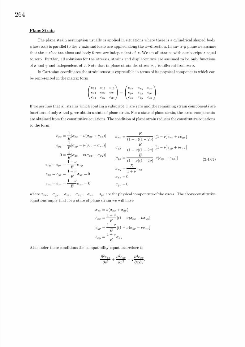
8/6/2019 Introduction to Tensor Calculus Continuum Mechanics - J. Heinbockel
http://slidepdf.com/reader/full/introduction-to-tensor-calculus-continuum-mechanics-j-heinbockel 270/372
264
Plane Strain
The plane strain assumption usually is applied in situations where there is a cylindrical shaped body
whose axis is parallel to the z axis and loads are applied along the z−direction. In any x-y plane we assume
that the surface tractions and body forces are independent of z. We set all strains with a subscript z equal
to zero. Further, all solutions for the stresses, strains and displacements are assumed to be only functionsof x and y and independent of z. Note that in plane strain the stress σzz is different from zero.
In Cartesian coordinates the strain tensor is expressible in terms of its physical components which can
be represented in the matrix form
e11 e12 e13
e21 e22 e23e31 e32 e33
=
exx exy exz
eyx eyy eyzezx ezy ezz
.
If we assume that all strains which contain a subscript z are zero and the remaining strain components are
functions of only x and y, we obtain a state of plane strain. For a state of plane strain, the stress components
are obtained from the constitutive equations. The condition of plane strain reduces the constitutive equations
to the form:
exx =1
E [σxx − ν (σyy + σzz)]
eyy =1
E [σyy − ν (σzz + σxx)]
0 =1
E [σzz − ν (σxx + σyy)]
exy = eyx =1 + ν
E σxy
ezy = eyz =1 + ν
E σyz = 0
ezx = exz = 1 + ν E σxz = 0
σxx =E
(1 + ν )(1 − 2ν )[(1 − ν )exx + νeyy ]
σyy =E
(1 + ν )(1 − 2ν )[(1 − ν )eyy + νexx]
σzz =E
(1 + ν )(1 − 2ν )[ν (eyy + exx)]
σxy =E
1 + ν exy
σxz = 0
σyz = 0
(2.4.63)
where σxx, σyy , σzz , σxy, σxz, σyz are the physical components of the stress. The above constitutive
equations imply that for a state of plane strain we will have
σzz = ν (σxx + σyy)
exx =1 + ν
E [(1 − ν )σxx − νσyy ]
eyy =1 + ν
E [(1 − ν )σyy − νσxx]
exy =1 + ν
E σxy.
Also under these conditions the compatibility equations reduce to
∂ 2exx∂y2
+∂ 2eyy∂x2
= 2∂ 2exy∂x∂y
.

8/6/2019 Introduction to Tensor Calculus Continuum Mechanics - J. Heinbockel
http://slidepdf.com/reader/full/introduction-to-tensor-calculus-continuum-mechanics-j-heinbockel 271/372
26
Plane Stress
An assumption of plane stress is usually applied to thin flat plates. The plate thinness is assumed to be
in the z−direction and loads are applied perpendicular to z. Under these conditions all stress components
with a subscript z are assumed to be zero. The remaining stress components are then treated as functions
of x and y.In Cartesian coordinates the stress tensor is expressible in terms of its physical components and can be
represented by the matrix σ11 σ12 σ13
σ21 σ22 σ23σ31 σ32 σ33
=
σxx σxy σxz
σyx σyy σyz
σzx σzy σzz
.
If we assume that all the stresses with a subscript z are zero and the remaining stresses are only functions of
x and y we obtain a state of plane stress. The constitutive equations simplify if we assume a state of plane
stress. These simplified equations are
exx =1
E σxx − ν
E σyy
eyy = 1E
σyy − ν E
σxx
ezz = − ν
E (σxx + σyy)
exy =1 + ν
E σxy
exz = 0
eyz = 0.
σxx =E
1
−ν 2
[exx + νeyy ]
σyy = E 1 − ν 2
[eyy + νexx]
σzz = 0 = (1 − ν )ezz + ν (exx + eyy)
σxy =E
1 + ν exy
σyz = 0
σxz = 0
(2.4.64)
For a state of plane stress the compatibility equations reduce to
∂ 2exx∂y2
+∂ 2eyy
∂x2= 2
∂ 2exy∂x∂y
(2.4.65)
and the three additional equations
∂ 2ezz∂x2
= 0,∂ 2ezz
∂y2= 0,
∂ 2ezz∂x∂y
= 0.
These three additional equations complicate the plane stress problem.
Airy Stress Function
In Cartesian coordinates we examine the equilibrium equations (2.4.25(b)) under the conditions of plane
strain. In terms of physical components we find that these equations reduce to
∂σxx
∂x+
∂σxy
∂y+ bx = 0,
∂σyx
∂x+
∂σyy
∂y+ by = 0,
∂σzz
∂z= 0.
The last equation is satisfied since σzz is a function of x and y. If we further assume that the body forces
are conservative and derivable from a potential function V by the operation b = −grad V or bi = −V ,i
we can express the above equilibrium equations in the form:
∂σxx
∂x+
∂σxy
∂y− ∂V
∂x= 0
∂σyx
∂x+
∂σyy
∂y− ∂V
∂y= 0
(2.4.66)
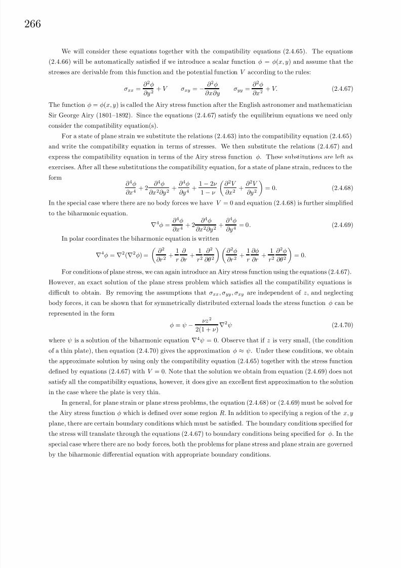
8/6/2019 Introduction to Tensor Calculus Continuum Mechanics - J. Heinbockel
http://slidepdf.com/reader/full/introduction-to-tensor-calculus-continuum-mechanics-j-heinbockel 272/372
266
We will consider these equations together with the compatibility equations (2.4.65). The equations
(2.4.66) will be automatically satisfied if we introduce a scalar function φ = φ(x, y) and assume that the
stresses are derivable from this function and the potential function V according to the rules:
σxx =∂ 2φ
∂y2+ V σxy = − ∂ 2φ
∂x∂yσyy =
∂ 2φ
∂x2+ V. (2.4.67)
The function φ = φ(x, y) is called the Airy stress function after the English astronomer and mathematician
Sir George Airy (1801–1892). Since the equations (2.4.67) satisfy the equilibrium equations we need only
consider the compatibility equation(s).
For a state of plane strain we substitute the relations (2.4.63) into the compatibility equation (2.4.65)
and write the compatibility equation in terms of stresses. We then substitute the relations (2.4.67) and
express the compatibility equation in terms of the Airy stress function φ. These substitutions are left as
exercises. After all these substitutions the compatibility equation, for a state of plane strain, reduces to the
form∂ 4φ
∂x4+ 2
∂ 4φ
∂x2∂y2+
∂ 4φ
∂y4+
1 − 2ν
1
−ν
∂ 2V
∂x2+
∂ 2V
∂y2 = 0. (2.4.68)
In the special case where there are no body forces we have V = 0 and equation (2.4.68) is further simplified
to the biharmonic equation.
∇4φ =∂ 4φ
∂x4+ 2
∂ 4φ
∂x2∂y2+
∂ 4φ
∂y4= 0. (2.4.69)
In polar coordinates the biharmonic equation is written
∇4φ = ∇2(∇2φ) =
∂ 2
∂r2+
1
r
∂
∂r+
1
r2∂ 2
∂θ2
∂ 2φ
∂r2+
1
r
∂φ
∂r+
1
r2∂ 2φ
∂θ2
= 0.
For conditions of plane stress, we can again introduce an Airy stress function using the equations (2.4.67).
However, an exact solution of the plane stress problem which satisfies all the compatibility equations is
difficult to obtain. By removing the assumptions that σxx, σyy , σxy are independent of z, and neglecting
body forces, it can be shown that for symmetrically distributed external loads the stress function φ can be
represented in the form
φ = ψ − νz2
2(1 + ν )∇2ψ (2.4.70)
where ψ is a solution of the biharmonic equation ∇4ψ = 0. Observe that if z is very small, (the condition
of a thin plate), then equation (2.4.70) gives the approximation φ ≈ ψ. Under these conditions, we obtain
the approximate solution by using only the compatibility equation (2.4.65) together with the stress function
defined by equations (2.4.67) with V = 0. Note that the solution we obtain from equation (2.4.69) does not
satisfy all the compatibility equations, however, it does give an excellent first approximation to the solution
in the case where the plate is very thin.
In general, for plane strain or plane stress problems, the equation (2.4.68) or (2.4.69) must be solved for
the Airy stress function φ which is defined over some region R. In addition to specifying a region of the x, y
plane, there are certain boundary conditions which must be satisfied. The boundary conditions specified for
the stress will translate through the equations (2.4.67) to boundary conditions being specified for φ. In the
special case where there are no body forces, both the problems for plane stress and plane strain are governed
by the biharmonic differential equation with appropriate boundary conditions.

8/6/2019 Introduction to Tensor Calculus Continuum Mechanics - J. Heinbockel
http://slidepdf.com/reader/full/introduction-to-tensor-calculus-continuum-mechanics-j-heinbockel 273/372
26
EXAMPLE 2.4-4 Assume there exist a state of plane strain with zero body forces. For F 11, F 12, F 22
constants, consider the function defined by
φ = φ(x, y) =1
2
F 22 x2 − 2F 12 xy + F 11 y2
.
This function is an Airy stress function because it satisfies the biharmonic equation ∇4
φ = 0. The resultingstress field is
σxx =∂ 2φ
∂y2= F 11 σyy =
∂ 2φ
∂x2= F 22 σxy = − ∂ 2φ
∂x∂y= F 12.
This example, corresponds to stresses on an infinite flat plate and illustrates a situation where all the stress
components are constants for all values of x and y. In this case, we have σzz = ν (F 11+F 22). The corresponding
strain field is obtained from the constitutive equations. We find these strains are
exx =1 + ν
E [(1 − ν )F 11 − νF 22] eyy =
1 + ν
E [(1 − ν )F 22 − νF 11] exy =
1 + ν
E F 12.
The displacement field is found to be
u = u(x, y) =1 + ν
E [(1 − ν )F 11 − νF 22] x +
1 + ν
E
F 12y + c1y + c2
v = v(x, y) =1 + ν
E [(1 − ν )F 22 − νF 11] y +
1 + ν
E
F 12x − c1x + c3,
with c1, c2, c3 constants, and is obtained by integrating the strain displacement equations given in Exercise
2.3, problem 2.
EXAMPLE 2.4-5. A special case from the previous example is obtained by setting F 22 = F 12 = 0.
This is the situation of an infinite plate with only tension in the x−direction. In this special case we have
φ =1
2F 11y2
. Changing to polar coordinates we write
φ = φ(r, θ) =F 11
2r2 sin2 θ =
F 114
r2(1 − cos2θ).
The Exercise 2.4, problem 20, suggests we utilize the Airy equations in polar coordinates and calculate the
stresses
σrr =1
r
∂φ
∂r+
1
r2∂ 2φ
∂θ2= F 11 cos2 θ =
F 112
(1 + cos 2θ)
σθθ =∂ 2φ
∂r2= F 11 sin2 θ =
F 112
(1 − cos2θ)
σrθ =1
r2∂φ
∂θ− 1
r
∂ 2φ
∂r∂θ= −F 11
2sin2θ.

8/6/2019 Introduction to Tensor Calculus Continuum Mechanics - J. Heinbockel
http://slidepdf.com/reader/full/introduction-to-tensor-calculus-continuum-mechanics-j-heinbockel 274/372
8/6/2019 Introduction to Tensor Calculus Continuum Mechanics - J. Heinbockel
http://slidepdf.com/reader/full/introduction-to-tensor-calculus-continuum-mechanics-j-heinbockel 275/372
26
The stresses are to remain bounded for all values of r and consequently we require c1 and c6 to be zero
to avoid infinite stresses for large values of r. The stress σrr |r=a = 0 requires that
2c2 +c3a2
= 0 and 2c5 + 6c7a4
+ 4c8a2
= 0.
The stress σrθ |r=a = 0 requires that2c5 − 6
c7a4
− 2c8a2
= 0.
In the limit as r → ∞ we require that the stresses must satisfy the boundary conditions from the previous
example 2.4-5. This leads to the equations 2c2 =F 11
2and 2c5 = −F 11
2. Solving the above system of equations
produces the Airy stress function
φ = φ(r, θ) =F 11
4+
F 114
r2 − a2
2F 11 ln r + c4 +
F 11a2
2− F 11
4r2 − F 11a4
4r2
cos2θ
and the corresponding stress field is
σrr = F 112
1 − a
2
r2
+ F 112
1 + 3 a
4
r4− 4 a
2
r2
cos2θ
σrθ = −F 112
1 − 3
a4
r4+ 2
a2
r2
sin2θ
σθθ =F 11
2
1 +
a2
r2
− F 11
2
1 + 3
a4
r4
cos2θ.
There is a maximum stress σθθ = 3F 11 at θ = π/2, 3π/2 and a minimum stress σθθ = −F 11 at θ = 0, π.
The effect of the circular hole has been to magnify the applied stress. The factor of 3 is known as a stress
concentration factor. In general, sharp corners and unusually shaped boundaries produce much higher stress
concentration factors than rounded boundaries.
EXAMPLE 2.4-7. Consider an infinite cylindrical tube, with inner radius R1 and the outer radius R0,
which is subjected to an internal pressure P 1 and an external pressure P 0 as illustrated in the figure 2.4-7.
Find the stress and displacement fields.
Solution: Let ur, uθ, uz denote the displacement field. We assume that uθ = 0 and uz = 0 since the
cylindrical surface r equal to a constant does not move in the θ or z directions. The displacement ur = ur(r)
is assumed to depend only upon the radial distance r. Under these conditions the Navier equations become
(λ + 2µ)d
dr
1
r
d
dr(rur)
= 0.
This equation has the solution ur = c1 r2
+ c2r
and the strain components are found from the relations
err =dur
dr, eθθ =
ur
r, ezz = erθ = erz = ezθ = 0.
The stresses are determined from Hooke’s law (the constitutive equations) and we write
σij = λδijΘ + 2µeij,
8/6/2019 Introduction to Tensor Calculus Continuum Mechanics - J. Heinbockel
http://slidepdf.com/reader/full/introduction-to-tensor-calculus-continuum-mechanics-j-heinbockel 276/372
270
where
Θ =∂ur
∂r+
ur
r=
1
r
∂
∂r(rur)
is the dilatation. These stresses are found to be
σrr = (λ + µ)c1−
2µ
r2
c2 σθθ = (λ + µ)c1 +2µ
r2
c2 σzz = λc1 σrθ = σrz = σzθ = 0.
We now apply the boundary conditions
σrr |r=R1nr = −
(λ + µ)c1 − 2µ
R21
c2
= +P 1 and σrr |r=R0
nr =
(λ + µ)c1 − 2µ
R20
c2
= −P 0.
Solving for the constants c1 and c2 we find
c1 =R21P 1 − R2
0P 0(λ + µ)(R2
0 − R21)
, c2 =R21R2
0(P 1 − P 0)
2µ(R20 − R2
1).
This produces the displacement field
ur = R21P 12(R2
0 − R21)
r
λ + µ+ R20
µr
− R20P 0
2(R20 − R2
1)
r
λ + µ+ R21
µr
, uθ = 0, uz = 0,
and stress fields
σrr =R21P 1
R20 − R2
1
1 − R2
0
r2
− R2
0P 0R20 − R2
1
1 − R2
1
r2
σθθ =R21P 1
R20 − R2
1
1 +
R20
r2
− R2
0P 0R20 − R2
1
1 +
R21
r2
σzz =
λ
λ + µ
R21P 1 − R2
0P 0R20 − R2
1
σrz = σzθ = σrθ = 0
EXAMPLE 2.4-8. By making simplifying assumptions the Navier equations can be reduced to a more
tractable form. For example, we can reduce the Navier equations to a one dimensional problem by making
the following assumptions
1. Cartesian coordinates x1 = x, x2 = y, x3 = z
2. u1 = u1(x, t), u2 = u3 = 0.
3. There are no body forces.
4. Initial conditions of u1(x, 0) = 0 and∂u1(x, 0)
∂t= 0
5. Boundary conditions of the displacement type u1(0, t) = f (t),
where f (t) is a specified function. These assumptions reduce the Navier equations to the single one dimen-
sional wave equation∂ 2u1∂t2
= α2 ∂ 2u1∂x2
, α2 =λ + 2µ
ρ.
The solution of this equation is
u1(x, t) =
f (t − x/α), x ≤ αt
0, x > αt.

8/6/2019 Introduction to Tensor Calculus Continuum Mechanics - J. Heinbockel
http://slidepdf.com/reader/full/introduction-to-tensor-calculus-continuum-mechanics-j-heinbockel 277/372
27
The solution represents a longitudinal elastic wave propagating in the x−direction with speed α. The stress
wave associated with this displacement is determined from the constitutive equations. We find
σxx = (λ + µ)exx = (λ + µ)∂u1
∂x.
This produces the stress wave
σxx =
− (λ+µ)α
f (t − x/α), x ≤ αt
0, x > αt.
Here there is a discontinuity in the stress wave front at x = αt.
Summary of Basic Equations of Elasticity
The equilibrium equations for a continuum have been shown to have the form σij,j + bi = 0, where
bi are the body forces per unit mass and σij is the stress tensor. In addition to the above equations we
have the constitutive equations σij = λekkδij + 2µeij which is a generalized Hooke’s law relating stress to
strain for a linear elastic isotropic material. The strain tensor is related to the displacement field ui by
the strain equations eij =1
2(ui,j + uj,i) . These equations can be combined to obtain the Navier equations
µui,jj + (λ + µ)uj,ji + bi = 0.
The above equations must be satisfied at all interior points of the material body. A boundary value
problem results when conditions on the displacement of the boundary are specified. That is, the Navier
equations must be solved subject to the prescribed displacement boundary conditions. If conditions on
the stress at the boundary are specified, then these prescribed stresses are called surface tractions and
must satisfy the relations ti (n) = σijnj , where ni is a unit outward normal vector to the boundary. For
surface tractions, we need to use the compatibility equations combined with the constitutive equations and
equilibrium equations. This gives rise to the Beltrami-Michell equations of compatibility
σij,kk +1
1 + ν σkk,ij + (bi,j + bj,i) +
ν
1 − ν bk,k = 0.
Here we must solve for the stress components throughout the continuum where the above equations hold
subject to the surface traction boundary conditions. Note that if an elasticity problem is formed in terms of
the displacement functions, then the compatibility equations can be ignored.
For mixed boundary value problems we must solve a system of equations consisting of the equilibrium
equations, constitutive equations, and strain displacement equations. We must solve these equations subject
to conditions where the displacements ui are prescribed on some portion(s) of the boundary and stresses are
prescribed on the remaining portion(s) of the boundary. Mixed boundary value problems are more difficultto solve.
For elastodynamic problems, the equilibrium equations are replaced by equations of motion. In this
case we need a set of initial conditions as well as boundary conditions before attempting to solve our basic
system of equations.
8/6/2019 Introduction to Tensor Calculus Continuum Mechanics - J. Heinbockel
http://slidepdf.com/reader/full/introduction-to-tensor-calculus-continuum-mechanics-j-heinbockel 278/372
272
EXERCISE 2.4
1. Verify the generalized Hooke’s law constitutive equations for hexagonal materials.
In the following problems the Young’s modulus E, Poisson’s ratio ν, the shear modulus or modulus
of rigidity µ (sometimes denoted by G in Engineering texts), Lame’s constant λ and the bulk modulus of elasticity k are assumed to satisfy the equations (2.4.19), (2.4.24) and (2.4.25). Show that these relations
imply the additional relations given in the problems 2 through 6.
2.
E =µ(3λ + 2µ)
µ + λ
E =λ(1 + ν )(1 − 2ν )
ν
E =9k(k − λ)
3k − λ
E = 2µ(1 + ν )
E =9kµ
µ + 3k
E = 3(1 − 2ν )k
3.
ν =3k − E
6k
ν = λ2(µ + λ)
ν = (E + λ)2 + 8λ2 − (E + λ)
4λ
ν =3k − 2µ
2(µ + 3k)
ν =E − 2µ
2µ
ν =λ
3k − λ
4.
k =
(E + λ)2 + 8λ2 + (E + 3λ)
6
k =2µ + 3λ
3
k =E
3(1 − 2ν )
k =µE
3(3µ − E )
k =2µ(1 + ν )
3(1 − 2ν )
k =λ(1 + ν )
3ν
5.
µ =3(k − λ)
2
µ =λ(1
−2ν )
2ν
µ =3k(1 − 2ν )
2(1 + ν )
µ = 3Ek9k − E
µ =
(E + λ)2 + 8λ2 + (E − 3λ)
4
µ =E
2(1 + ν )
6.
λ =3kν
1 + ν
λ =µ(2µ − E )
E − 3µ
λ =3k − 2µ
3
λ =3k(3k − E )
9k − E
λ =νE
(1 + ν )(1 − 2ν )
λ =2µν
1 − 2ν
7. The previous exercises 2 through 6 imply that the generalized Hooke’s law
σij = 2µeij + λδijekk
is expressible in a variety of forms. From the set of constants (µ,λ,ν ,E ,k) we can select any two constants
and then express Hooke’s law in terms of these constants.
(a) Express the above Hooke’s law in terms of the constants E and ν.
(b) Express the above Hooke’s law in terms of the constants k and E.
(c) Express the above Hooke’s law in terms of physical components. Hint: The quantity ekk is an invariant
hence all you need to know is how second order tensors are represented in terms of physical components.
See also problems 10,11,12.
8/6/2019 Introduction to Tensor Calculus Continuum Mechanics - J. Heinbockel
http://slidepdf.com/reader/full/introduction-to-tensor-calculus-continuum-mechanics-j-heinbockel 279/372
27
8. Verify the equations defining the stress for plane strain in Cartesian coordinates are
σxx =E
(1 + ν )(1 − 2ν )[(1 − ν )exx + νeyy ]
σyy =E
(1 + ν )(1
−2ν )
[(1 − ν )eyy + νexx]
σzz = Eν (1 + ν )(1 − 2ν )
[exx + eyy ]
σxy =E
1 + ν exy
σyz = σxz = 0
9. Verify the equations defining the stress for plane strain in polar coordinates are
σrr =E
(1 + ν )(1 − 2ν )[(1 − ν )err + νeθθ ]
σθθ =E
(1 + ν )(1−
2ν )[(1 − ν )eθθ + νerr ]
σzz =νE
(1 + ν )(1 − 2ν )[err + eθθ]
σrθ =E
1 + ν erθ
σrz = σθz = 0
10. Write out the independent components of Hooke’s generalized law for strain in terms of stress, and
stress in terms of strain, in Cartesian coordinates. Express your results using the parameters ν and E.
(Assume a linear elastic, homogeneous, isotropic material.)
11. Write out the independent components of Hooke’s generalized law for strain in terms of stress, and
stress in terms of strain, in cylindrical coordinates. Express your results using the parameters ν and E.
(Assume a linear elastic, homogeneous, isotropic material.)
12. Write out the independent components of Hooke’s generalized law for strain in terms of stress, and
stress in terms of strain in spherical coordinates. Express your results using the parameters ν and E. (Assume
a linear elastic, homogeneous, isotropic material.)
13. For a linear elastic, homogeneous, isotropic material assume there exists a state of plane strain in
Cartesian coordinates. Verify the equilibrium equations are
∂σxx
∂x
+∂σxy
∂y
+ bx = 0
∂σyx
∂x+
∂σyy
∂y+ by = 0
∂σzz
∂z+ bz = 0
Hint: See problem 14, Exercise 2.3.
8/6/2019 Introduction to Tensor Calculus Continuum Mechanics - J. Heinbockel
http://slidepdf.com/reader/full/introduction-to-tensor-calculus-continuum-mechanics-j-heinbockel 280/372
274
14 . For a linear elastic, homogeneous, isotropic material assume there exists a state of plane strain in
polar coordinates. Verify the equilibrium equations are
∂σrr
∂r+
1
r
∂σrθ
∂θ+
1
r(σrr − σθθ) + br = 0
∂σrθ
∂r +
1
r
∂σθθ
∂θ +
2
r σrθ + bθ = 0∂σzz
∂z+ bz = 0
Hint: See problem 15, Exercise 2.3.
15. For a linear elastic, homogeneous, isotropic material assume there exists a state of plane stress in
Cartesian coordinates. Verify the equilibrium equations are
∂σxx
∂x+
∂σxy
∂y+ bx = 0
∂σyx
∂x+
∂σyy
∂y+ by = 0
16. Determine the compatibility equations in terms of the Airy stress function φ when there exists a state
of plane stress. Assume the body forces are derivable from a potential function V.
17. For a linear elastic, homogeneous, isotropic material assume there exists a state of plane stress in
polar coordinates. Verify the equilibrium equations are
∂σrr
∂r+
1
r
∂σrθ
∂θ+
1
r(σrr − σθθ) + br = 0
∂σrθ
∂r+
1
r
∂σθθ
∂θ+
2
rσrθ + bθ = 0
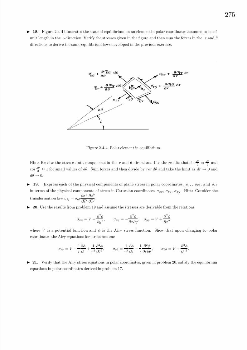
8/6/2019 Introduction to Tensor Calculus Continuum Mechanics - J. Heinbockel
http://slidepdf.com/reader/full/introduction-to-tensor-calculus-continuum-mechanics-j-heinbockel 281/372
27
18. Figure 2.4-4 illustrates the state of equilibrium on an element in polar coordinates assumed to be of
unit length in the z-direction. Verify the stresses given in the figure and then sum the forces in the r and θ
directions to derive the same equilibrium laws developed in the previous exercise.
Figure 2.4-4. Polar element in equilibrium.
Hint: Resolve the stresses into components in the r and θ directions. Use the results that sin dθ2
≈ dθ2 and
cos dθ2 ≈ 1 for small values of dθ. Sum forces and then divide by rdr dθ and take the limit as dr → 0 and
dθ → 0.
19. Express each of the physical components of plane stress in polar coordinates, σrr , σθθ , and σrθ
in terms of the physical components of stress in Cartesian coordinates σxx, σyy , σxy . Hint: Consider the
transformation law σij = σab
∂xa
∂xi
∂xb
∂xj.
20. Use the results from problem 19 and assume the stresses are derivable from the relations
σxx = V +∂ 2φ
∂y2, σxy = − ∂ 2φ
∂x∂y, σyy = V +
∂ 2φ
∂x2
where V is a potential function and φ is the Airy stress function. Show that upon changing to polar
coordinates the Airy equations for stress become
σrr = V + 1r
∂φ∂r
+ 1r2
∂ 2φ∂θ2
, σrθ = 1r2
∂φ∂θ
− 1r
∂ 2φ∂r∂θ
, σθθ = V + ∂ 2φ∂r2
.
21. Verify that the Airy stress equations in polar coordinates, given in problem 20, satisfy the equilibrium
equations in polar coordinates derived in problem 17.

8/6/2019 Introduction to Tensor Calculus Continuum Mechanics - J. Heinbockel
http://slidepdf.com/reader/full/introduction-to-tensor-calculus-continuum-mechanics-j-heinbockel 282/372
276
22. In Cartesian coordinates show that the traction boundary conditions, equations (2.3.11), can be
written in terms of the constants λ and µ as
T 1 = λn1ekk + µ
2n1
∂u1
∂x1+ n2
∂u1
∂x2+
∂u2
∂x1
+ n3
∂u1
∂x3+
∂u3
∂x1
T 2 = λn2ekk + µ
n1∂u2
∂x1 +∂u1
∂x2
+ 2n2
∂u2
∂x2 + n3∂u2
∂x3 +∂u3
∂x2
T 3 = λn3ekk + µ
n1
∂u3
∂x1+
∂u1
∂x3
+ n2
∂u3
∂x2+
∂u2
∂x3
+ 2n3
∂u3
∂x3
where (n1, n2, n3) are the direction cosines of the unit normal to the surface, u1, u2, u3 are the components
of the displacements and T 1, T 2, T 3 are the surface tractions.
23. Consider an infinite plane subject to tension in the x−direction only. Assume a state of plane strain
and let σxx = T with σxy = σyy = 0. Find the strain components exx, eyy and exy. Also find the displacement
field u = u(x, y) and v = v(x, y).
24. Consider an infinite plane subject to tension in the y-direction only. Assume a state of plane strainand let σyy = T with σxx = σxy = 0. Find the strain components exx, eyy and exy. Also find the displacement
field u = u(x, y) and v = v(x, y).
25. Consider an infinite plane subject to tension in both the x and y directions. Assume a state of plane
strain and let σxx = T , σyy = T and σxy = 0. Find the strain components exx, eyy and exy. Also find the
displacement field u = u(x, y) and v = v(x, y).
26. An infinite cylindrical rod of radius R0 has an external pressure P 0 as illustrated in figure 2.5-5. Find
the stress and displacement fields.
Figure 2.4-5. External pressure on a rod.

8/6/2019 Introduction to Tensor Calculus Continuum Mechanics - J. Heinbockel
http://slidepdf.com/reader/full/introduction-to-tensor-calculus-continuum-mechanics-j-heinbockel 283/372
27
Figure 2.4-6. Internal pressure on circular hole.
Figure 2.4-7. Tube with internal and external pressure.
27. An infinite plane has a circular hole of radius R1 with an internal pressure P 1 as illustrated in thefigure 2.4-6. Find the stress and displacement fields.
28. A tube of inner radius R1 and outer radius R0 has an internal pressure of P 1 and an external pressure
of P 0 as illustrated in the figure 2.4-7. Verify the stress and displacement fields derived in example 2.4-7.
29. Use Cartesian tensors and combine the equations of equilibrium σij,j + bi = 0, Hooke’s law σij =
λekkδij + 2µeij and the strain tensor eij =1
2(ui,j + uj,i) and derive the Navier equations of equilibrium
σij,j + bi = (λ + µ)∂ Θ
∂xi+ µ
∂ 2ui
∂xk∂xk+ bi = 0,
where Θ = e11 + e22 + e33 is the dilatation.
30. Show the Navier equations in problem 29 can be written in the tensor form
µui,jj + (λ + µ)uj,ji + bi = 0
or the vector form
µ∇2u + (λ + µ)∇ (∇ · u) + b = 0.

8/6/2019 Introduction to Tensor Calculus Continuum Mechanics - J. Heinbockel
http://slidepdf.com/reader/full/introduction-to-tensor-calculus-continuum-mechanics-j-heinbockel 284/372
278
31. Show that in an orthogonal coordinate system the components of ∇(∇ · u) can be expressed in terms
of physical components by the relation
[∇ (∇ · u)]i =1
hi
∂
∂xi
1
h1h2h3
∂ (h2h3u(1))
∂x1+
∂ (h1h3u(2))
∂x2+
∂ (h1h2u(3))
∂x3
32. Show that in orthogonal coordinates the components of ∇2
u can be written∇2ui
= gjkui,jk = Ai
and in terms of physical components one can write
hiA(i) =3
j=1
1
h2j
∂ 2(hiu(i))
∂xj∂xj− 2
3m=1
m
i j
∂ (hmu(m))
∂xj−
3m=1
m
j j
∂ (hiu(i))
∂xm
−3
m=1
hmu(m)
∂
∂xj
m
i j
−
3 p=1
m
i p
p
j j
−
3 p=1
m
j p
p
i j
33. Use the results in problem 32 to show in Cartesian coordinates the physical components of [∇2u]i = Ai
can be represented ∇2 u · e1 = A(1) =
∂ 2u
∂x2+
∂ 2u
∂y2+
∂ 2u
∂z2
∇2 u · e2 = A(2) =
∂ 2v
∂x2+
∂ 2v
∂y2+
∂ 2v
∂z2
∇2 u · e3 = A(3) =
∂ 2w
∂x2+
∂ 2w
∂y2+
∂ 2w
∂z2
where (u, v, w) are the components of the displacement vector u.
34. Use the results in problem 32 to show in cylindrical coordinates the physical components of [∇2u]i = Ai
can be represented ∇2u · er = A(1) = ∇2ur − 1
r2ur − 2
r2∂uθ
∂θ∇2 u · eθ = A(2) = ∇2uθ +
2
r2∂ur
∂θ− 1
r2uθ∇2u
· ez = A(3) = ∇2uz
where ur, uθ, uz are the physical components of u and ∇2α =∂ 2α
∂r2+
1
r
∂α
∂r+
1
r2∂ 2α
∂θ2+
∂ 2α
∂z2
35. Use the results in problem 32 to show in spherical coordinates the physical components of [∇2u]i = Ai
can be represented
∇2u
· eρ = A(1) = ∇2uρ − 2
ρ2uρ − 2
ρ2∂uθ
∂θ− 2cot θ
ρ2uθ − 2
ρ2 sin θ
∂uφ
∂φ∇2u · eθ = A(2) = ∇2uθ + 2
ρ2∂uρ
∂θ− 1
ρ2 sin θuθ − 2cos θ
ρ2 sin2 θ∂uθ
∂φ∇2u · eφ = A(3) = ∇2uφ − 1
ρ2 sin2 θuφ +
2
ρ2 sin θ
∂uρ
∂φ+
2cos θ
ρ2 sin2 θ
∂uθ
∂φ
where uρ, uθ, uφ are the physical components of u and where
∇2α =∂ 2α
∂ρ2+
2
ρ
∂α
∂ρ+
1
ρ2∂ 2α
∂θ2+
cot θ
ρ2∂α
∂θ+
1
ρ2 sin2 θ
∂ 2α
∂φ2

8/6/2019 Introduction to Tensor Calculus Continuum Mechanics - J. Heinbockel
http://slidepdf.com/reader/full/introduction-to-tensor-calculus-continuum-mechanics-j-heinbockel 285/372
27
36. Combine the results from problems 30,31,32 and 33 and write the Navier equations of equilibrium
in Cartesian coordinates. Alternatively, write the stress-strain relations (2.4.29(b)) in terms of physical
components and then use these results, together with the results from Exercise 2.3, problems 2 and 14, to
derive the Navier equations.
37. Combine the results from problems 30,31,32 and 34 and write the Navier equations of equilibrium
in cylindrical coordinates. Alternatively, write the stress-strain relations (2.4.29(b)) in terms of physical
components and then use these results, together with the results from Exercise 2.3, problems 3 and 15, to
derive the Navier equations.
38. Combine the results from problems 30,31,32 and 35 and write the Navier equations of equilibrium
in spherical coordinates. Alternatively, write the stress-strain relations (2.4.29(b)) in terms of physical
components and then use these results, together with the results from Exercise 2.3, problems 4 and 16, to
derive the Navier equations.
39. Assume b = −grad V and let φ denote the Airy stress function defined by
σxx =V +
∂ 2φ
∂y2
σyy =V +∂ 2φ
∂x2
σxy = − ∂ 2φ
∂x∂y
(a) Show that for conditions of plane strain the equilibrium equations in two dimensions are satisfied by the
above definitions. (b) Express the compatibility equation
∂ 2exx∂y2
+∂ 2eyy
∂x2= 2
∂ 2exy∂x∂y
in terms of φ and V and show that
∇4φ +
1 − 2ν
1 − ν ∇2V = 0.
40. Consider the case where the body forces are conservative and derivable from a scalar potential function
such that bi = −V ,i. Show that under conditions of plane strain in rectangular Cartesian coordinates the
compatibility equation e11,22 + e22,11 = 2e12,12 can be reduced to the form ∇2σii =1
1 − ν ∇2V , i = 1, 2
involving the stresses and the potential. Hint: Differentiate the equilibrium equations.
41. Use the relation σij = 2µeij + λemmδij and solve for the strain in terms of the stress.
42. Derive the equation (2.4.26) from the equation (2.4.23).
43. In two dimensions assume that the body forces are derivable from a potential function V and
bi = −gijV ,j . Also assume that the stress is derivable from the Airy stress function and the potential
function by employing the relations σij = imjn um,n + gijV i, j, m, n = 1, 2 where um = φ ,m and
pq is the two dimensional epsilon permutation symbol and all indices have the range 1,2.
(a) Show that imjn (φm) ,nj = 0.
(b) Show that σij,j = −bi.
(c) Verify the stress laws for cylindrical and Cartesian coordinates given in problem 20 by using the above
expression for σij . Hint: Expand the contravariant derivative and convert all terms to physical compo-
nents. Also recall that ij = 1√ g
eij .
8/6/2019 Introduction to Tensor Calculus Continuum Mechanics - J. Heinbockel
http://slidepdf.com/reader/full/introduction-to-tensor-calculus-continuum-mechanics-j-heinbockel 286/372
280
44. Consider a material with body forces per unit volume ρF i, i = 1, 2, 3 and surface tractions denoted by
σr = σrjnj , where nj is a unit surface normal. Further, let δui denote a small displacement vector associated
with a small variation in the strain δeij.
(a) Show the work done during a small variation in strain is δW = δW B + δW S where δW B =
V
ρF iδui dτ
is a volume integral representing the work done by the body forces and δW S = S
σr
δur dS is a surfaceintegral representing the work done by the surface forces.
(b) Using the Gauss divergence theorem show that the work done can be represented as
δW =1
2
V
cijmnδ[emneij] dτ or W =1
2
V
σijeij dτ.
The scalar quantity 12σijeij is called the strain energy density or strain energy per unit volume.
Hint: Interchange subscripts, add terms and calculate 2W = V
σij [δui,j + δuj,i] dτ.
45. Consider a spherical shell subjected to an internal pressure pi and external pressure po. Let a denote
the inner radius and b the outer radius of the spherical shell. Find the displacement and stress fields in
spherical coordinates (ρ,θ,φ).Hint: Assume symmetry in the θ and φ directions and let the physical components of displacements satisfy
the relations uρ = uρ(ρ), uθ = uφ = 0.
46. (a) Verify the average normal stress is proportional to the dilatation, where the proportionality
constant is the bulk modulus of elasticity. i.e. Show that 13σi
i = E1−2ν
13eii = keii where k is the bulk modulus
of elasticity.
(b) Define the quantities of strain deviation and stress deviation in terms of the average normal stress
s = 13
σii and average cubic dilatation e = 1
3eii as follows
strain deviator εij = eij
−eδij
stress deviator sij = σij − sδij
Show that zero results when a contraction is performed on the stress and strain deviators. (The above
definitions are used to split the strain tensor into two parts. One part represents pure dilatation and
the other part represents pure distortion.)
(c) Show that (1 − 2ν )s = Ee or s = (3λ + 2µ)e
(d) Express Hooke’s law in terms of the strain and stress deviator and show
E (εij + eδij) = (1 + ν )sij + (1 − 2ν )sδij
which simplifies to sij = 2µεij .
47. Show the strain energy density (problem 44) can be written in terms of the stress and strain deviators
(problem 46) and
W =1
2
V
σijeij dτ =1
2
V
(3se + sijεij) dτ
and from Hooke’s law
W =3
2
V
((3λ + 2µ)e2 +2µ
3εijεij) dτ.
8/6/2019 Introduction to Tensor Calculus Continuum Mechanics - J. Heinbockel
http://slidepdf.com/reader/full/introduction-to-tensor-calculus-continuum-mechanics-j-heinbockel 287/372
28
48. Find the stress σrr ,σrθ and σθθ in an infinite plate with a small circular hole, which is traction free,
when the plate is subjected to a pure shearing force F 12. Determine the maximum stress.
49. Show that in terms of E and ν
C 1111 =E (1 − ν )
(1 + ν )(1 − 2ν )
C 1122 =Eν
(1 + ν )(1 − 2ν )
C 1212 =E
2(1 + ν )
50. Show that in Cartesian coordinates the quantity
S = σxxσyy + σyyσzz + σzzσxx − (σxy)2 − (σyz )2 − (σxz)2
is a stress invariant. Hint: First verify that in tensor form S =1
2(σiiσjj − σijσij).
51. Show that in Cartesian coordinates for a state of plane strain where the displacements are given by
u = u(x, y),v = v(x, y) and w = 0, the stress components must satisfy the equations
∂σxx
∂x+
∂σxy
∂y+ bx =0
∂σyx
∂x+
∂σyy
∂y+ by =0
∇2(σxx + σyy) =−
1 − ν
∂bx∂x
+∂by∂y
52. Show that in Cartesian coordinates for a state of plane stress where σxx = σxx(x, y), σyy = σyy(x, y),
σxy = σxy(x, y) and σxz = σyz = σzz = 0 the stress components must satisfy
∂σxx
∂x+
∂σxy
∂y+ bx =0
∂σyx
∂x
+∂σyy
∂y
+ by =0
∇2(σxx + σyy) = − (ν + 1)
∂bx∂x
+∂by∂y

8/6/2019 Introduction to Tensor Calculus Continuum Mechanics - J. Heinbockel
http://slidepdf.com/reader/full/introduction-to-tensor-calculus-continuum-mechanics-j-heinbockel 288/372
282
§2.5 CONTINUUM MECHANICS (FLUIDS)
Let us consider a fluid medium and use Cartesian tensors to derive the mathematical equations that
describe how a fluid behaves. A fluid continuum, like a solid continuum, is characterized by equations
describing:
1. Conservation of linear momentumσij,j + bi = vi (2.5.1)
2. Conservation of angular momentum σij = σji .
3. Conservation of mass (continuity equation)
∂
∂t+
∂
∂xivi +
∂vi∂xi
= 0 orD
Dt+ ∇ · V = 0. (2.5.2)
In the above equations vi, i = 1, 2, 3 is a velocity field, is the density of the fluid, σij is the stress tensor
and bj is an external force per unit mass. In the cgs system of units of measurement, the above quantities
have dimensions
[vj ] = cm/sec2, [bj ] = dynes/g, [σij ] = dyne/cm2, [] = g/cm3. (2.5.3)
The displacement field ui, i = 1, 2, 3 can be represented in terms of the velocity field vi, i = 1, 2, 3, by
the relation
ui =
t0
vi dt. (2.5.4)
The strain tensor components of the medium can then be represented in terms of the velocity field as
eij =1
2(ui,j + uj,i) =
t0
1
2(vi,j + vj,i) dt =
t0
Dij dt, (2.5.5)
where
Dij =1
2(vi,j + vj,i) (2.5.6)
is called the rate of deformation tensor , velocity strain tensor , or rate of strain tensor.
Note the difference in the equations describing a solid continuum compared with those for a fluid
continuum. In describing a solid continuum we were primarily interested in calculating the displacement
field ui, i = 1, 2, 3 when the continuum was subjected to external forces. In describing a fluid medium, we
calculate the velocity field vi, i = 1, 2, 3 when the continuum is subjected to external forces. We therefore
replace the strain tensor relations by the velocity strain tensor relations in all future considerations concerning
the study of fluid motion.
Constitutive Equations for Fluids
In addition to the above basic equations, we will need a set of constitutive equations which describe the
material properties of the fluid. Toward this purpose consider an arbitrary point within the fluid medium
and pass an imaginary plane through the point. The orientation of the plane is determined by a unit normal
ni , i = 1, 2, 3 to the planar surface. For a fluid at rest we wish to determine the stress vector t(n)i acting
on the plane element passing through the selected point P. We desire to express t(n)i in terms of the stress
tensor σij . The superscript (n) on the stress vector is to remind you that the stress acting on the planar
element depends upon the orientation of the plane through the point.
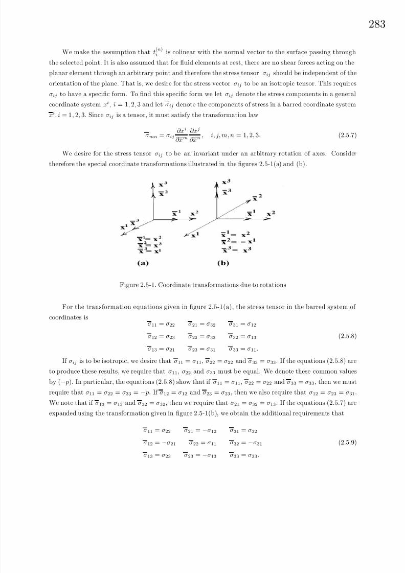
8/6/2019 Introduction to Tensor Calculus Continuum Mechanics - J. Heinbockel
http://slidepdf.com/reader/full/introduction-to-tensor-calculus-continuum-mechanics-j-heinbockel 289/372
28
We make the assumption that t(n)i is colinear with the normal vector to the surface passing through
the selected point. It is also assumed that for fluid elements at rest, there are no shear forces acting on the
planar element through an arbitrary point and therefore the stress tensor σij should be independent of the
orientation of the plane. That is, we desire for the stress vector σij to be an isotropic tensor. This requires
σij to have a specific form. To find this specific form we let σij denote the stress components in a general
coordinate system xi, i = 1, 2, 3 and let σij denote the components of stress in a barred coordinate system
xi, i = 1, 2, 3. Since σij is a tensor, it must satisfy the transformation law
σmn = σij∂xi
∂xm∂xj
∂xn, i, j, m, n = 1, 2, 3. (2.5.7)
We desire for the stress tensor σij to be an invariant under an arbitrary rotation of axes. Consider
therefore the special coordinate transformations illustrated in the figures 2.5-1(a) and (b).
Figure 2.5-1. Coordinate transformations due to rotations
For the transformation equations given in figure 2.5-1(a), the stress tensor in the barred system of
coordinates isσ11 = σ22 σ21 = σ32 σ31 = σ12
σ12 = σ23 σ22 = σ33 σ32 = σ13
σ13 = σ21 σ23 = σ31 σ33 = σ11.
(2.5.8)
If σij is to be isotropic, we desire that σ11 = σ11, σ22 = σ22 and σ33 = σ33. If the equations (2.5.8) are
to produce these results, we require that σ11, σ22 and σ33 must be equal. We denote these common values
by (− p). In particular, the equations (2.5.8) show that if σ11 = σ11, σ22 = σ22 and σ33 = σ33, then we must
require that σ11 = σ22 = σ33 = − p. If σ12 = σ12 and σ23 = σ23, then we also require that σ12 = σ23 = σ31.
We note that if σ13 = σ13 and σ32 = σ32, then we require that σ21 = σ32 = σ13. If the equations (2.5.7) are
expanded using the transformation given in figure 2.5-1(b), we obtain the additional requirements that
σ11 = σ22 σ21 = −σ12 σ31 = σ32
σ12 = −σ21 σ22 = σ11 σ32 = −σ31
σ13 = σ23 σ23 = −σ13 σ33 = σ33.
(2.5.9)

8/6/2019 Introduction to Tensor Calculus Continuum Mechanics - J. Heinbockel
http://slidepdf.com/reader/full/introduction-to-tensor-calculus-continuum-mechanics-j-heinbockel 290/372
284
Analysis of these equations implies that if σij is to be isotropic, then σ21 = σ21 = −σ12 = −σ21
or σ21 = 0 which implies σ12 = σ23 = σ31 = σ21 = σ32 = σ13 = 0. (2.5.10)
The above analysis demonstrates that if the stress tensor σij is to be isotropic, it must have the form
σij = − pδij . (2.5.11)
Use the traction condition (2.3.11), and express the stress vector as
t(n)j = σijni = − pnj. (2.5.12)
This equation is interpreted as representing the stress vector at a point on a surface with outward unit
normal ni, where p is the pressure (hydrostatic pressure) stress magnitude assumed to be positive. The
negative sign in equation (2.5.12) denotes a compressive stress.
Imagine a submerged object in a fluid medium. We further imagine the object to be covered with unit
normal vectors emanating from each point on its surface. The equation (2.5.12) shows that the hydrostatic
pressure always acts on the object in a compressive manner. A force results from the stress vector acting on
the object. The direction of the force is opposite to the direction of the unit outward normal vectors. It is
a compressive force at each point on the surface of the object.
The above considerations were for a fluid at rest (hydrostatics). For a fluid in motion (hydrodynamics)
a different set of assumptions must be made. Hydrodynamical experiments show that the shear stress
components are not zero and so we assume a stress tensor having the form
σij = − pδij + τ ij , i, j = 1, 2, 3, (2.5.13)
where τ ij is called the viscous stress tensor. Note that all real fluids are both viscous and compressible.
Definition: (Viscous/inviscid fluid) If the viscous stress ten-
sor τ ij is zero for all i,j, then the fluid is called an inviscid, non-
viscous, ideal or perfect fluid. The fluid is called viscous when τ ij
is different from zero.
In these notes it is assumed that the equation (2.5.13) represents the basic form for constitutive equations
describing fluid motion.
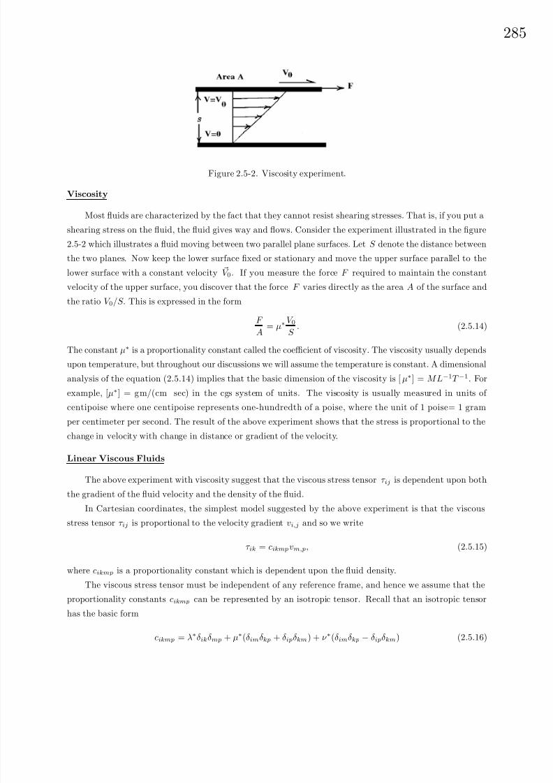
8/6/2019 Introduction to Tensor Calculus Continuum Mechanics - J. Heinbockel
http://slidepdf.com/reader/full/introduction-to-tensor-calculus-continuum-mechanics-j-heinbockel 291/372
28
Figure 2.5-2. Viscosity experiment.
Viscosity
Most fluids are characterized by the fact that they cannot resist shearing stresses. That is, if you put a
shearing stress on the fluid, the fluid gives way and flows. Consider the experiment illustrated in the figure
2.5-2 which illustrates a fluid moving between two parallel plane surfaces. Let S denote the distance between
the two planes. Now keep the lower surface fixed or stationary and move the upper surface parallel to the
lower surface with a constant velocity V 0. If you measure the force F required to maintain the constantvelocity of the upper surface, you discover that the force F varies directly as the area A of the surface and
the ratio V 0/S. This is expressed in the form
F
A= µ∗
V 0S
. (2.5.14)
The constant µ∗ is a proportionality constant called the coefficient of viscosity. The viscosity usually depends
upon temperature, but throughout our discussions we will assume the temperature is constant. A dimensional
analysis of the equation (2.5.14) implies that the basic dimension of the viscosity is [µ∗] = ML−1T −1. For
example, [µ∗] = gm/(cm sec) in the cgs system of units. The viscosity is usually measured in units of
centipoise where one centipoise represents one-hundredth of a poise, where the unit of 1 poise= 1 gramper centimeter per second. The result of the above experiment shows that the stress is proportional to the
change in velocity with change in distance or gradient of the velocity.
Linear Viscous Fluids
The above experiment with viscosity suggest that the viscous stress tensor τ ij is dependent upon both
the gradient of the fluid velocity and the density of the fluid.
In Cartesian coordinates, the simplest model suggested by the above experiment is that the viscous
stress tensor τ ij is proportional to the velocity gradient vi,j and so we write
τ ik = cikmpvm,p, (2.5.15)
where cikmp is a proportionality constant which is dependent upon the fluid density.
The viscous stress tensor must be independent of any reference frame, and hence we assume that the
proportionality constants cikmp can be represented by an isotropic tensor. Recall that an isotropic tensor
has the basic form
cikmp = λ∗δikδmp + µ∗(δimδkp + δipδkm) + ν ∗(δimδkp − δipδkm) (2.5.16)

8/6/2019 Introduction to Tensor Calculus Continuum Mechanics - J. Heinbockel
http://slidepdf.com/reader/full/introduction-to-tensor-calculus-continuum-mechanics-j-heinbockel 292/372
286
where λ∗, µ∗ and ν ∗ are constants. Examining the results from equations (2.5.11) and (2.5.13) we find that if
the viscous stress is symmetric, then τ ij = τ ji. This requires ν ∗ be chosen as zero. Consequently, the viscous
stress tensor reduces to the form
τ ik = λ∗δikv p,p + µ∗(vk,i + vi,k). (2.5.17)
The coefficient µ∗
is called the first coefficient of viscosity and the coefficient λ∗
is called the second coefficientof viscosity. Sometimes it is convenient to define
ζ = λ∗ +2
3µ∗ (2.5.18)
as “another second coefficient of viscosity,” or “bulk coefficient of viscosity.” The condition of zero bulk
viscosity is known as Stokes hypothesis. Many fluids problems assume the Stoke’s hypothesis. This requires
that the bulk coefficient be zero or very small. Under these circumstances the second coefficient of viscosity
is related to the first coefficient of viscosity by the relation λ∗ = −23µ∗. In the study of shock waves and
acoustic waves the Stoke’s hypothesis is not applicable.
There are many tables and empirical formulas where the viscosity of different types of fluids or gasescan be obtained. For example, in the study of the kinetic theory of gases the viscosity can be calculated
from the Sutherland formula µ∗ =C 1gT 3/2
T + C 2where C 1, C 2 are constants for a specific gas. These constants
can be found in certain tables. The quantity g is the gravitational constant and T is the temperature in
degrees Rankine (oR = 460 + oF ). Many other empirical formulas like the above exist. Also many graphs
and tabular values of viscosity can be found. The table 5.1 lists the approximate values of the viscosity of
some selected fluids and gases.
Table 5.1
Viscosity of selected fluids and gasesin units of
gramcm−sec = Poise
at Atmospheric Pressure.Substance 0C 20C 60C 100C
Water 0.01798 0.01002 0.00469 0.00284Alcohol 0.01773
Ethyl Alcohol 0.012 0.00592Glycol 0.199 0.0495 0.0199
Mercury 0.017 0.0157 0.013 0.0100Air 1.708(10−4) 2.175(10−4)
Helium 1.86(10−4) 1.94(10−4) 2.28(10−4)
Nitrogen 1.658(10−4) 1.74(10−4) 1.92(10−4) 2.09(10−4)
The viscous stress tensor given in equation (2.5.17) may also be expressed in terms of the rate of
deformation tensor defined by equation (2.5.6). This representation is
τ ij = λ∗δijDkk + 2µ∗Dij , (2.5.19)
where 2Dij = vi,j + vj,i and Dkk = D11 + D22 + D33 = v1,1 + v2,2 + v3,3 = vi,i = Θ is the rate of change
of the dilatation considered earlier. In Cartesian form, with velocity components u,v,w, the viscous stress

8/6/2019 Introduction to Tensor Calculus Continuum Mechanics - J. Heinbockel
http://slidepdf.com/reader/full/introduction-to-tensor-calculus-continuum-mechanics-j-heinbockel 293/372
28
tensor components are
τ xx =(λ∗ + 2µ∗)∂u
∂x+ λ∗
∂v
∂y+∂w
∂z
τ yy =(λ∗ + 2µ∗)
∂v
∂y+ λ∗
∂u
∂x+∂w
∂z
τ zz =(λ
∗
+ 2µ
∗
)
∂w
∂z + λ
∗∂u∂x +
∂v
∂y
τ yx = τ xy =µ∗∂u
∂y+∂v
∂x
τ zx = τ xz =µ∗
∂w
∂x+∂u
∂z
τ zy = τ yz =µ
∗ ∂v∂z +
∂w
∂y In cylindrical form, with velocity components vr, vθ, vz, the viscous stess tensor components are
τ rr =2µ∗∂vr
∂r+ λ∗∇ · V
τ θθ =2µ∗
1
r
∂vθ
∂θ+vr
r
+ λ∗∇ · V
τ zz =2µ∗∂vz
∂z+ λ∗∇ · V
where ∇ · V =1
r
∂
∂r(rvr) +
1
r
∂vθ
∂θ+∂vz
∂z
τ θr = τ rθ =µ∗
1
r
∂vr
∂θ+∂vθ
∂r−vθ
r
τ rz = τ zr =µ∗
∂vr
∂z+∂vz
∂r
τ zθ = τ θz =µ∗
1
r
∂vz
∂θ+∂vθ
∂z
In spherical coordinates, with velocity components vρ, vθ, vφ, the viscous stress tensor components have the
form
τ ρρ =2µ∗∂vρ
∂ρ+ λ∗∇ · V
τ θθ =2µ∗
1
ρ
∂vθ
∂θ+vρ
ρ
+ λ∗∇ · V
τ φφ =2µ∗
1
ρ sin θ
∂vφ
∂φ+vρ
ρ+vθ cot θ
ρ
+ λ∗∇ · V
where ∇ · V =1
ρ2∂
∂ρ
ρ2vρ
+
1
ρ sin θ
∂
∂θ(sin θvθ) +
1
ρ sin θ
∂vφ
∂φ
τ ρθ = τ θρ =µ∗ρ∂
∂ρ
vθ
ρ
+
1
ρ
∂vρ
∂θ
τ φρ = τ ρφ =µ∗
1
ρ sin θ
∂vr
∂φ+ ρ
∂
∂ρ
vθ
ρ
τ θφ = τ φθ =µ∗
sin θ
ρ
∂
∂θ
vφ
sin θ
+
1
ρ sin θ
∂vθ
∂φ
Note that the viscous stress tensor is a linear function of the rate of deformation tensor Dij . Such a
fluid is called a Newtonian fluid. In cases where the viscous stress tensor is a nonlinear function of Dij the
fluid is called non-Newtonian.
Definition: (Newtonian Fluid) If the viscous stress tensor τ ij
is expressible as a linear function of the rate of deformation tensor
Dij , the fluid is called a Newtonian fluid. Otherwise, the fluid is
called a non-Newtonian fluid.
Important note: Do not assume an arbitrary form for the constitutive equations unless there is ex-
perimental evidence to support your assumption. A constitutive equation is a very important step in the
modeling processes as it describes the material you are working with. One cannot arbitrarily assign a form
to the viscous stress and expect the mathematical equations to describe the correct fluid behavior. The form
of the viscous stress is an important part of the modeling process and by assigning different forms to the
viscous stress tensor then various types of materials can be modeled. We restrict our study in these notes
to Newtonian fluids.
In Cartesian coordinates the rate of deformation-stress constitutive equations for a Newtonian fluid can
be written as
σij = − pδij + λ∗δijDkk + 2µ∗Dij (2.5.20)

8/6/2019 Introduction to Tensor Calculus Continuum Mechanics - J. Heinbockel
http://slidepdf.com/reader/full/introduction-to-tensor-calculus-continuum-mechanics-j-heinbockel 294/372
288
which can also be written in the alternative form
σij = − pδij + λ∗δijvk,k + µ∗(vi,j + vj,i) (2.5.21)
involving the gradient of the velocity.
Upon transforming from a Cartesian coordinate system yi
, i = 1, 2, 3 to a more general system of coordinates xi, i = 1, 2, 3, we write
σmn = σij∂y i
∂xm∂y j
∂xn. (2.5.22)
Now using the divergence from equation (2.1.3) and substituting equation (2.5.21) into equation (2.5.22) we
obtain a more general expression for the constitutive equation. Performing the indicated substitutions there
results
σmn =− pδij + λ∗δijvk,k + µ∗(vi,j + vj,i)
∂y i
∂xm∂yj
∂xn
σmn = − pgmn + λ∗gmnvk,k + µ∗(vm,n + vn,m).
Dropping the bar notation, the stress-velocity strain relationships in the general coordinates xi, i = 1, 2, 3, is
σmn = − pgmn + λ∗gmngikvi,k + µ∗(vm,n + vn,m). (2.5.23)
Summary
The basic equations which describe the motion of a Newtonian fluid are :
Continuity equation (Conservation of mass)
∂
∂t+
vi,i
= 0, orD
Dt+ ∇ · V = 0 1 equation. (2.5.24)
Conservation of linear momentum σij,j + bi = vi, 3 equations
or in vector form D V
Dt= b + ∇ ·σ = b − ∇ p + ∇ ·τ (2.5.25)
where σ =3
i=1
3j=1(− pδij + τ ij) ei ej and τ =
3i=1
3j=1 τ ij ei ej are second order tensors. Conser-
vation of angular momentum σij = σji, (Reduces the set of equations (2.5.23) to 6 equations.) Rate of
deformation tensor (Velocity strain tensor)
Dij =1
2(vi,j + vj,i) , 6 equations. (2.5.26)
Constitutive equations
σmn = − pgmn + λ∗gmngikvi,k + µ∗(vm,n + vn,m), 6 equations. (2.5.27)
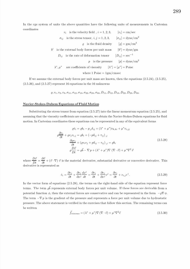
8/6/2019 Introduction to Tensor Calculus Continuum Mechanics - J. Heinbockel
http://slidepdf.com/reader/full/introduction-to-tensor-calculus-continuum-mechanics-j-heinbockel 295/372
28
In the cgs system of units the above quantities have the following units of measurements in Cartesian
coordinatesvi is the velocity field , i = 1, 2, 3, [vi] = cm/sec
σij is the stress tensor, i, j = 1, 2, 3, [σij ] = dyne/cm2
is the fluid density [] = gm/cm3
bi is the external body forces per unit mass [bi] = dyne/gm
Dij is the rate of deformation tensor [Dij] = sec−1
p is the pressure [ p] = dyne/cm2
λ∗, µ∗ are coefficients of viscosity [λ∗] = [µ∗] = Poise
where 1 Poise = 1gm/cmsec
If we assume the external body forces per unit mass are known, then the equations (2.5.24), (2.5.25),
(2.5.26), and (2.5.27) represent 16 equations in the 16 unknowns
, v1
, v2
, v3
, σ11
, σ12
, σ13
, σ22
, σ23
, σ33
, D11
, D12
, D13
, D22
, D23
, D33
.
Navier-Stokes-Duhem Equations of Fluid Motion
Substituting the stress tensor from equation (2.5.27) into the linear momentum equation (2.5.25), and
assuming that the viscosity coefficients are constants, we obtain the Navier-Stokes-Duhem equations for fluid
motion. In Cartesian coordinates these equations can be represented in any of the equivalent forms
vi = bi − p,jδij + (λ∗ + µ∗)vk,ki + µ∗vi,jj
∂vi∂t
+ vjvi,j = bi + (− pδij + τ ij) ,j
∂vi∂t
+ (vivj + pδij − τ ij) ,j = bi
Dv
Dt= b − ∇ p + (λ∗ + µ∗)∇ (∇ · v) + µ∗∇2 v
(2.5.28)
whereDv
Dt=
∂v
∂t+ (v · ∇) v is the material derivative, substantial derivative or convective derivative. This
derivative is represented as
vi =∂vi∂t
+∂vi∂xj
dxj
dt=
∂vi∂t
+∂vi∂xj
vj =∂vi∂t
+ vi,jvj . (2.5.29)
In the vector form of equations (2.5.28), the terms on the right-hand side of the equation represent force
terms. The term b represents external body forces per unit volume. If these forces are derivable from apotential function φ, then the external forces are conservative and can be represented in the form −∇ φ.
The term −∇ p is the gradient of the pressure and represents a force per unit volume due to hydrostatic
pressure. The above statement is verified in the exercises that follow this section. The remaining terms can
be written
f viscous = (λ∗ + µ∗)∇ (∇ · v) + µ∗∇2v (2.5.30)

8/6/2019 Introduction to Tensor Calculus Continuum Mechanics - J. Heinbockel
http://slidepdf.com/reader/full/introduction-to-tensor-calculus-continuum-mechanics-j-heinbockel 296/372
290
and are given the physical interpretation of an internal force per unit volume. These internal forces arise
from the shearing stresses in the moving fluid. If f viscous is zero the vector equation in (2.5.28) is called
Euler’s equation.
If the viscosity coefficients are nonconstant, then the Navier-Stokes equations can be written in the
Cartesian form
[∂vi∂t
+ vj∂vi∂xj
] =bi +∂
∂xj
− pδij + λ∗δij
∂vk∂xk
+ µ∗
∂vi∂xj
+∂vj∂xi
=bi − ∂p
∂xi+
∂
∂xi
λ∗
∂vk∂xk
+
∂
∂xj
µ∗
∂vi∂xj
+∂vj∂xi
which can also be written in terms of the bulk coefficient of viscosity ζ = λ∗ + 2
3µ∗ as
[∂vi∂t
+ vj∂vi∂xj
] =bi − ∂p
∂xi+
∂
∂xi
(ζ − 2
3µ∗)
∂vk∂xk
+
∂
∂xj
µ∗
∂vi∂xj
+∂vj∂xi
=bi − ∂p
∂xi+
∂
∂xi ζ
∂vk∂xk
+∂
∂xj µ∗
∂vi∂xj
+∂vj∂xi
− 2
3δij
∂vk∂xk
These equations form the basics of viscous flow theory.
In the case of orthogonal coordinates, where g(i)(i) = h2i (no summation) and gij = 0 for i = j, general
expressions for the Navier-Stokes equations in terms of the physical components v(1), v(2), v(3) are:
Navier-Stokes-Duhem equations for compressible fluid in terms of physical components: (i = j = k)
∂v(i)
∂t+v(1)
h1
∂v(i)
∂x1+v(2)
h2
∂v(i)
∂x2+v(3)
h3
∂v(i)
∂x3
−v( j)
hihj v( j)
∂hj
∂xi− v(i)
∂hi
∂xj+
v(k)
hihk v(i)
∂hi
∂xk− v(k)
∂hk
∂xi =
b(i)
hi−
1
hi
∂p
∂xi+
1
hi
∂
∂xi
λ∗∇ · V
+
µ∗
hihj
hjhi
∂
∂xi
v( j)
hj
+hi
hj
∂
∂xj
v(i)
hi
∂hi∂hj
+µ∗
hihk
hi
hk
∂
∂xk
v(i)
hi
+hk
hi
∂
∂xi
v(k)
hk
∂hi
∂xk−
2µ∗
hihj
1
hj
∂v( j)
∂xj+
v(k)
hjhk
∂hj
∂xk+
v(i)
hihj
∂hj
∂xi
−
2µ∗
hihk
1
hk
∂v(k)
∂xk+
v(i)
hihk
∂hk
∂xi+
v(k)
hkhj
∂hk
∂xi
∂hk
∂xi+
1
hihjhk
∂
∂xi
2µ∗hjhk
1
hi
∂v(i)
∂xi+
v( j)
hihj
∂hi
∂hj+
v(k)
hihk
∂hi
∂xk
+
∂
∂xj
µ∗hihk
hj
hi
∂
∂xi
v( j)
hj
+hi
hj
∂
∂xj
v(i)
hi
+
∂
∂xk
µ∗hihj
hi
hk
∂
∂xk
v(i)
hi
+hk
hi
∂
∂xi
v(k)
hk
(2.5.31)
where ∇ · v is found in equation (2.1.4).
In the above equation, cyclic values are assigned to i, j and k. That is, for the x1 components assign
the values i = 1, j = 2, k = 3; for the x2 components assign the values i = 2, j = 3, k = 1; and for the x3
components assign the values i = 3, j = 1, k = 2.
The tables 5.2, 5.3 and 5.4 show the expanded form of the Navier-Stokes equations in Cartesian, cylin-
drical and spherical coordinates respectively.
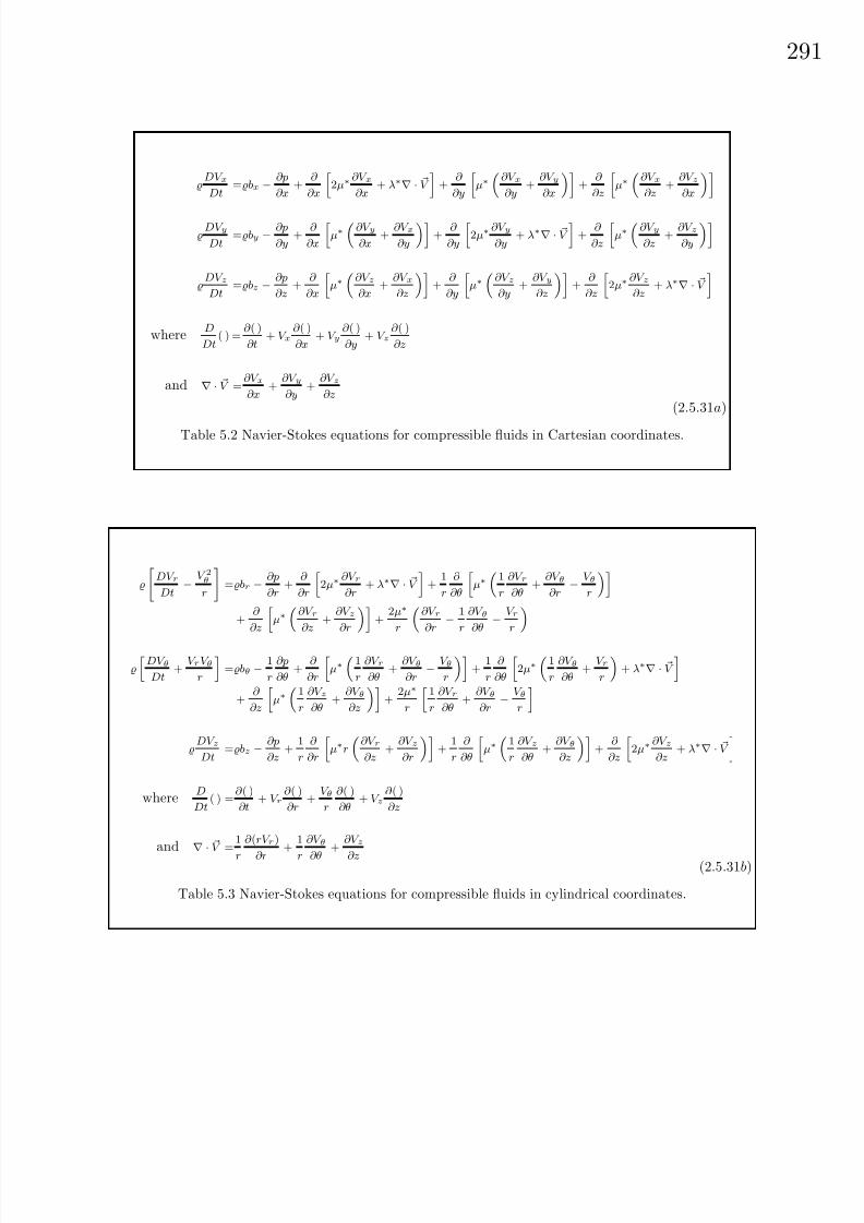
8/6/2019 Introduction to Tensor Calculus Continuum Mechanics - J. Heinbockel
http://slidepdf.com/reader/full/introduction-to-tensor-calculus-continuum-mechanics-j-heinbockel 297/372
29
DV x
Dt=bx −
∂p
∂x+
∂
∂x
2µ∗
∂V x
∂x+ λ∗∇ · V
+
∂
∂y
µ∗
∂V x
∂y+∂V y
∂x
+
∂
∂z
µ∗
∂V x
∂z+∂V z
∂x
DV y
Dt=by −
∂p
∂y+
∂
∂x
µ∗∂V y
∂x+∂V x
∂y
+
∂
∂y
2µ∗
∂V y
∂y+ λ∗∇ · V
+
∂
∂z
µ∗∂V y
∂z+∂V z
∂y
DV z
Dt=bz −
∂p
∂z+
∂
∂x
µ∗∂V z
∂x+∂V x
∂z
+
∂
∂y
µ∗∂V z
∂y+∂V y
∂z
+
∂
∂z
2µ∗
∂V z
∂z+ λ∗∇ · V
whereD
Dt( ) =
∂ ( )
∂t+ V x
∂ ( )
∂x+ V y
∂ ( )
∂y+ V z
∂ ( )
∂z
and ∇ · V =∂V x
∂x+∂V y
∂y+∂V z
∂z
(2.5.31a)
Table 5.2 Navier-Stokes equations for compressible fluids in Cartesian coordinates.
DV r
Dt−V 2θ
r
=br −
∂p
∂r+
∂
∂r
2µ∗
∂V r
∂r+ λ∗∇ · V
+
1
r
∂
∂θ
µ∗
1
r
∂V r
∂θ+∂V θ
∂r−V θ
r
+
∂
∂z µ∗
∂V r
∂z+∂V z
∂r +
2µ∗
r ∂V r
∂r−
1
r
∂V θ
∂θ−V r
r
DV θ
Dt+V rV θ
r
=bθ −
1
r
∂p
∂θ+
∂
∂r
µ∗
1
r
∂V r
∂θ+∂V θ
∂r−V θ
r
+
1
r
∂
∂θ
2µ∗
1
r
∂V θ
∂θ+V r
r
+ λ∗∇ · V
+
∂
∂z
µ∗
1
r
∂V z
∂θ+∂V θ
∂z
+
2µ∗
r
1
r
∂V r
∂θ+∂V θ
∂r−V θ
r
DV z
Dt=bz −
∂p
∂z+
1
r
∂
∂r
µ∗r
∂V r
∂z+∂V z
∂r
+
1
r
∂
∂θ
µ∗
1
r
∂V z
∂θ+∂V θ
∂z
+
∂
∂z
2µ∗
∂V z
∂z+ λ∗∇ · V
whereD
Dt( ) =
∂ ( )
∂t+ V r
∂ ( )
∂r+V θ
r
∂ ( )
∂θ+ V z
∂ ( )
∂z
and ∇ · V =1
r
∂ (rV r)
∂r
+1
r
∂V θ
∂θ
+∂V z
∂z (2.5.31b)
Table 5.3 Navier-Stokes equations for compressible fluids in cylindrical coordinates.
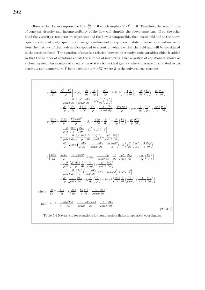
8/6/2019 Introduction to Tensor Calculus Continuum Mechanics - J. Heinbockel
http://slidepdf.com/reader/full/introduction-to-tensor-calculus-continuum-mechanics-j-heinbockel 298/372
292
Observe that for incompressible flow DDt = 0 which implies ∇ · V = 0. Therefore, the assumptions
of constant viscosity and incompressibility of the flow will simplify the above equations. If on the other
hand the viscosity is temperature dependent and the flow is compressible, then one should add to the above
equations the continuity equation, an energy equation and an equation of state. The energy equation comes
from the first law of thermodynamics applied to a control volume within the fluid and will be considered
in the sections ahead. The equation of state is a relation between thermodynamic variables which is added
so that the number of equations equals the number of unknowns. Such a system of equations is known as
a closed system. An example of an equation of state is the ideal gas law where pressure p is related to gas
density and temperature T by the relation p = RT where R is the universal gas constant.
DV ρ
Dt−
V 2θ + V 2φ
ρ
= bρ −
∂p
∂ρ+
∂
∂ρ
2µ∗
∂V ρ
∂ρ+ λ∗∇ · V
+
1
ρ
∂
∂θ
µ∗ρ
∂
∂ρ
V θ
ρ
+µ∗
ρ
∂V ρ
∂θ
+
1
ρ sin θ
∂
∂φ µ∗
ρ sin θ
∂V ρ
∂φ + µ∗
ρ
∂
∂ρ V φρ +µ∗
ρ
4∂V ρ
∂ρ−
2
ρ
∂V θ
∂θ−
4V ρ
ρ−
2
ρ sin θ
∂V φ
∂φ−
2V θ cot θ
ρ+ ρ cot θ
∂
∂ρ
V θ
ρ
+
cot θ
ρ
∂V ρ
∂θ
DV θ
Dt+
V ρV θ
ρ−
V 2φ
cot θ
ρ
= bθ −
1
ρ
∂p
∂θ+
∂
∂ρ
µ∗ρ
∂
∂ρ
V θ
ρ
+µ∗
ρ
∂V ρ
∂θ
+
1
ρ
∂
∂θ
2µ∗
ρ
∂V θ
∂θ+ V ρ
+ λ∗∇ · V
+
1
ρ sin θ
∂
∂φ
µ∗ sin θ
ρ
∂
∂θ
V φ
sin θ
+
µ∗
ρ sin θ
∂V θ
∂φ
+µ∗
ρ
2cot θ
1
ρ
∂V θ
∂θ−
1
ρ sin θ
∂V φ
∂φ−V θ cot θ
ρ
+ 3
ρ∂
∂ρ
V θ
ρ
+
1
ρ
∂V ρ
∂θ
DV φDt
+V θV φ
ρ+V θV φ cot θ
ρ
= bφ −
1
ρ sin θ
∂p
∂φ+
∂
∂ρ
µ∗
ρ sin θ
∂V ρ
∂φ+ µ∗ρ
∂
∂ρ
V φρ
+
1
ρ
∂
∂θ
µ∗ sin θ
ρ
∂
∂θ
V φ
sin θ
+
µ∗
ρ sin θ
∂V θ
∂φ
+
1
ρ sin θ
∂
∂φ
2µ∗
ρ
1
sin θ
∂V φ
∂φ+ V ρ + V θ cot θ
+ λ∗∇ · V
+µ∗
ρ
3
ρ sin θ
∂V ρ
∂φ+ 3ρ
∂
∂ρ
V φ
ρ
+ 2 cot θ
sin θ
ρ
∂
∂θ
V φ
sin θ
+
1
ρ sin θ
∂V θ
∂φ
whereD
Dt( ) =
∂ ( )
∂t+ V ρ
∂ ( )
∂ρ+V θ
ρ
∂ ( )
∂θ+
V φ
ρ sin θ
∂ ( )
∂φ
and ∇ · V = 1ρ2
∂ (ρ
2
V ρ)∂ρ
+ 1ρ sin θ
∂V θ sin θ∂θ
+ 1ρ sin θ
∂V φ
∂φ
(2.5.31c)
Table 5.4 Navier-Stokes equations for compressible fluids in spherical coordinates.
8/6/2019 Introduction to Tensor Calculus Continuum Mechanics - J. Heinbockel
http://slidepdf.com/reader/full/introduction-to-tensor-calculus-continuum-mechanics-j-heinbockel 299/372
29
We now consider various special cases of the Navier-Stokes-Duhem equations.
Special Case 1: Assume that b is a conservative force such that b = −∇ φ. Also assume that the viscous
force terms are zero. Consider steady flow ( ∂v∂t = 0) and show that equation (2.5.28) reduces to the equation
(v · ∇) v =−1
∇ p − ∇ φ is constant. (2.5.32)
Employing the vector identity
(v · ∇) v = (∇ × v) × v +1
2∇(v · v), (2.5.33)
we take the dot product of equation (2.5.32) with the vector v. Noting that v · [(∇ × v) × v] = 0 we obtain
v · ∇
p
+ φ +
1
2v2
= 0. (2.5.34)
This equation shows that for steady flow we will have
p
+ φ +
1
2v2 = constant (2.5.35)
along a streamline. This result is known as Bernoulli’s theorem. In the special case where φ = gh is a
force due to gravity, the equation (2.5.35) reduces top
+
v2
2+ gh = constant. This equation is known as
Bernoulli’s equation. It is a conservation of energy statement which has many applications in fluids.
Special Case 2: Assume that b = −∇ φ is conservative and define the quantity Ω by
Ω = ∇ × v = curl v ω =1
2Ω (2.5.36)
as the vorticity vector associated with the fluid flow and observe that its magnitude is equivalent to twice
the angular velocity of a fluid particle. Then using the identity from equation (2.5.33) we can write the
Navier-Stokes-Duhem equations in terms of the vorticity vector. We obtain the hydrodynamic equations
∂v
∂t+ Ω × v +
1
2∇ v2 = − 1
∇ p − ∇ φ +
1
f viscous, (2.5.37)
where f viscous is defined by equation (2.5.30). In the special case of nonviscous flow this further reduces to
the Euler equation∂v
∂t+ Ω × v +
1
2∇ v2 = − 1
∇ p − ∇ φ.
If the density is a function of the pressure only it is customary to introduce the function
P = p
c
dp
so that ∇P =
dP
dp∇ p =
1
∇ p
then the Euler equation becomes
∂v
∂t+ Ω × v = −∇(P + φ +
1
2v2).
Some examples of vorticies are smoke rings, hurricanes, tornadoes, and some sun spots. You can create
a vortex by letting water stand in a sink and then remove the plug. Watch the water and you will see that
a rotation or vortex begins to occur. Vortices are associated with circulating motion.

8/6/2019 Introduction to Tensor Calculus Continuum Mechanics - J. Heinbockel
http://slidepdf.com/reader/full/introduction-to-tensor-calculus-continuum-mechanics-j-heinbockel 300/372
294
Pick an arbitrary simple closed curve C and place it in the fluid flow and define the line integral
K =
C
v · et ds, where ds is an element of arc length along the curve C, v is the vector field defining the
velocity, and et is a unit tangent vector to the curve C. The integral K is called the circulation of the fluid
around the closed curve C. The circulation is the summation of the tangential components of the velocity
field along the curve C. The local vorticity at a point is defined as the limit
limArea→0
Circulation around C
Area inside C = circulation per unit area.
By Stokes theorem, if curl v = 0, then the fluid is called irrotational and the circulation is zero. Otherwise
the fluid is rotational and possesses vorticity.
If we are only interested in the velocity field we can eliminate the pressure by taking the curl of both
sides of the equation (2.5.37). If we further assume that the fluid is incompressible we obtain the special
equations∇ · v = 0 Incompressible fluid, is constant.
Ω = curl v Definition of vorticity vector.
∂ Ω
∂t+ ∇ × ( Ω × v) =
µ∗
∇2 Ω Results because curl of gradient is zero.
(2.5.38)
Note that when Ω is identically zero, we have irrotational motion and the above equations reduce to the
Cauchy-Riemann equations. Note also that if the term ∇ × ( Ω × v) is neglected, then the last equation in
equation (2.5.38) reduces to a diffusion equation. This suggests that the vorticity diffuses through the fluid
once it is created.
Vorticity can be caused by a rigid rotation or by shear flow. For example, in cylindrical coordinates let
V = rω eθ, with r, ω constants, denote a rotational motion, then curl V = ∇ × V = 2ω ez, which shows the
vorticity is twice the rotation vector. Shear can also produce vorticity. For example, consider the velocity
field V = y e1 with y ≥ 0. Observe that this type of flow produces shear because |
V | increases as y increases.
For this flow field we have curl V = ∇ × V = − e3. The right-hand rule tells us that if an imaginary paddle
wheel is placed in the flow it would rotate clockwise because of the shear effects.
Scaled Variables
In the Navier-Stokes-Duhem equations for fluid flow we make the assumption that the external body
forces are derivable from a potential function φ and write b = −∇ φ [dyne/gm] We also want to write the
Navier-Stokes equations in terms of scaled variables
v =v
v0
p = p p0
=
0
t = tτ
φ =φ
gL,
x = xL
y =y
L
z = zL
which can be referred to as the barred system of dimensionless variables. Dimensionless variables are intro-
duced by scaling each variable associated with a set of equations by an appropriate constant term called a
characteristic constant associated with that variable. Usually the characteristic constants are chosen from
various parameters used in the formulation of the set of equations. The characteristic constants assigned to
each variable are not unique and so problems can be scaled in a variety of ways. The characteristic constants
8/6/2019 Introduction to Tensor Calculus Continuum Mechanics - J. Heinbockel
http://slidepdf.com/reader/full/introduction-to-tensor-calculus-continuum-mechanics-j-heinbockel 301/372
29
assigned to each variable are scales, of the appropriate dimension, which act as reference quantities which
reflect the order of magnitude changes expected of that variable over a certain range or area of interest
associated with the problem. An inappropriate magnitude selected for a characteristic constant can result
in a scaling where significant information concerning the problem can be lost. This is analogous to selecting
an inappropriate mesh size in a numerical method. The numerical method might give you an answer but
details of the answer might be lost.
In the above scaling of the variables occurring in the Navier-Stokes equations we let v0 denote some
characteristic speed, p0 a characteristic pressure, 0 a characteristic density, L a characteristic length, g the
acceleration of gravity and τ a characteristic time (for example τ = L/v0), then the barred variables v, p,
,φ, t, x, y and z are dimensionless. Define the barred gradient operator by
∇ =∂
∂xe1 +
∂
∂ye2 +
∂
∂ze3
where all derivatives are with respect to the barred variables. The above change of variables reduces the
Navier-Stokes-Duhem equations
∂v
∂t+ (v · ∇) v = −∇φ − ∇ p + (λ∗ + µ∗)∇ (∇ · v) + µ∗∇2 v, (2.5.39)
to the form0v0
τ
∂ v
∂t+
0v20
L
v · ∇ v = −0g∇ φ − p0
L
∇ p
+(λ∗ + µ∗)
L2v0∇
∇ · v
+
µ∗v0
L2
∇2 v.
(2.5.40)
Now if each term in the equation (2.5.40) is divided by the coefficient 0v20/L, we obtain the equation
S∂ v∂t
+ v · ∇ v =
−1F
∇ φ − E ∇ p +λ∗
µ∗+ 1
1R
∇ ∇ · v
+1R
∇2 v (2.5.41)
which has the dimensionless coefficients
E =p0
0v20= Euler number
F =v20gL
= Froude number, g is acceleration of gravity
R =0V 0L
µ∗= Reynolds number
S =L
τv0= Strouhal number.
Dropping the bars over the symbols, we write the dimensionless equation using the above coefficients.
The scaled equation is found to have the form
S∂v
∂t+ (v · ∇)v = − 1
F ∇φ − E ∇ p +
λ∗
µ∗+ 1
1
R∇ (∇ · v) +
1
R∇2v (2.5.42)
8/6/2019 Introduction to Tensor Calculus Continuum Mechanics - J. Heinbockel
http://slidepdf.com/reader/full/introduction-to-tensor-calculus-continuum-mechanics-j-heinbockel 302/372
296
Boundary Conditions
Fluids problems can be classified as internal flows or external flows. An example of an internal flow
problem is that of fluid moving through a converging-diverging nozzle. An example of an external flow
problem is fluid flow around the boundary of an aircraft. For both types of problems there is some sort of
boundary which influences how the fluid behaves. In these types of problems the fluid is assumed to adhereto a boundary. Let rb denote the position vector to a point on a boundary associated with a moving fluid,
and let r denote the position vector to a general point in the fluid. Define v(r) as the velocity of the fluid at
the point r and define v(rb) as the known velocity of the boundary. The boundary might be moving within
the fluid or it could be fixed in which case the velocity at all points on the boundary is zero. We define the
boundary condition associated with a moving fluid as an adherence boundary condition.
Definition: (Adherence Boundary Condition)
An adherence boundary condition associated with a fluid in motion
is defined as the limit limr→rb
v(r) = v(rb) where rb is the position
vector to a point on the boundary.
Sometimes, when no finite boundaries are present, it is necessary to impose conditions on the components
of the velocity far from the origin. Such conditions are referred to as boundary conditions at infinity.
Summary and Additional Considerations
Throughout the development of the basic equations of continuum mechanics we have neglected ther-
modynamical and electromagnetic effects. The inclusion of thermodynamics and electromagnetic fields adds
additional terms to the basic equations of a continua. These basic equations describing a continuum are:
Conservation of massThe conservation of mass is a statement that the total mass of a body is unchanged during its motion.
This is represented by the continuity equation
∂
∂t+ (vk),k = 0 or
D
Dt+ ∇ · V = 0
where is the mass density and vk is the velocity.
Conservation of linear momentum
The conservation of linear momentum requires that the time rate of change of linear momentum equal
the resultant of all forces acting on the body. In symbols, we write
D
Dt
V
vi dτ = S
F i(s)ni dS + V
F i(b) dτ +n
α=1
F i(α) (2.5.43)
where Dvi
Dt = ∂vi
∂t + ∂vi
∂xkvk is the material derivative, F i(s) are the surface forces per unit area, F i(b) are the
body forces per unit mass and F i(α) represents isolated external forces. Here S represents the surface and
V represents the volume of the control volume. The right-hand side of this conservation law represents the
resultant force coming from the consideration of all surface forces and body forces acting on a control volume.
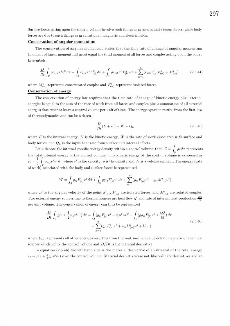
8/6/2019 Introduction to Tensor Calculus Continuum Mechanics - J. Heinbockel
http://slidepdf.com/reader/full/introduction-to-tensor-calculus-continuum-mechanics-j-heinbockel 303/372
29
Surface forces acting upon the control volume involve such things as pressures and viscous forces, while body
forces are due to such things as gravitational, magnetic and electric fields.
Conservation of angular momentum
The conservation of angular momentum states that the time rate of change of angular momentum
(moment of linear momentum) must equal the total moment of all forces and couples acting upon the body.
In symbols,
D
Dt
V
eijkxjvk dτ =
S
eijkxjF k(s) dS +
V
eijkxjF k(b) dτ +n
α=1
(eijkxj(α)F k(α) + M i(α)) (2.5.44)
where M i(α) represents concentrated couples and F k(α) represents isolated forces.
Conservation of energy
The conservation of energy law requires that the time rate of change of kinetic energy plus internal
energies is equal to the sum of the rate of work from all forces and couples plus a summation of all external
energies that enter or leave a control volume per unit of time. The energy equation results from the first law
of thermodynamics and can be written
D
Dt(E + K ) = W + Qh (2.5.45)
where E is the internal energy, K is the kinetic energy, W is the rate of work associated with surface and
body forces, and Qh is the input heat rate from surface and internal effects.
Let e denote the internal specific energy density within a control volume, then E =
V
edτ represents
the total internal energy of the control volume. The kinetic energy of the control volume is expressed as
K =1
2
V
gijvivj dτ where vi is the velocity, is the density and dτ is a volume element. The energy (rate
of work) associated with the body and surface forces is represented
W =
S
gijF i(s)vj dS +
V
gijF i(b)vj dτ +n
α=1
(gijF i(α)vj + gijM i(α)ωj)
where ωj is the angular velocity of the point xi(α), F i(α) are isolated forces, and M i(α) are isolated couples.
Two external energy sources due to thermal sources are heat flow qi and rate of internal heat production ∂Q∂t
per unit volume. The conservation of energy can thus be represented
D
Dt
V
(e +1
2gijvivj) dτ =
S
(gijF i(s)vj − qini) dS +
V
(gijF i(b)vj +∂Q
∂t) dτ
+
n
α=1(gijF i
(α)
vj + gijM i
(α)
ωj + U (α))
(2.5.46)
where U (α) represents all other energies resulting from thermal, mechanical, electric, magnetic or chemical
sources which influx the control volume and D/Dt is the material derivative.
In equation (2.5.46) the left hand side is the material derivative of an integral of the total energy
et = (e + 12gijvivj) over the control volume. Material derivatives are not like ordinary derivatives and so

8/6/2019 Introduction to Tensor Calculus Continuum Mechanics - J. Heinbockel
http://slidepdf.com/reader/full/introduction-to-tensor-calculus-continuum-mechanics-j-heinbockel 304/372
298
we cannot interchange the order of differentiation and integration in this term. Here we must use the result
thatD
Dt
V
et dτ =
V
∂et∂t
+ ∇ · (et V )
dτ.
To prove this result we consider a more general problem. Let A denote the amount of some quantity per
unit mass. The quantity A can be a scalar, vector or tensor. The total amount of this quantity inside thecontrol volume is A =
V
A dτ and therefore the rate of change of this quantity is
∂A
∂t=
V
∂ (A)
∂tdτ =
D
Dt
V
A dτ − S
A V · ndS,
which represents the rate of change of material within the control volume plus the influx into the control
volume. The minus sign is because n is always a unit outward normal. By converting the surface integral to
a volume integral, by the Gauss divergence theorem, and rearranging terms we find that
D
Dt
V
A dτ =
V
∂ (A)
∂t+ ∇ · (A V )
dτ.
In equation (2.5.46) we neglect all isolated external forces and substitute F i(s) = σijnj , F i(b) = bi where
σij = − pδij + τ ij . We then replace all surface integrals by volume integrals and find that the conservation of
energy can be represented in the form
∂et∂t
+ ∇ · (et V ) = ∇(σ · V ) − ∇ · q + b · V +∂Q
∂t(2.5.47)
where et = e + (v21 + v22 + v23)/2 is the total energy and σ =3
i=1
3j=1 σij ei ej is the second order stress
tensor. Here
σ · V = − p V +
3
j=1τ 1jvj e1 +
3
j=1τ 2jvj e2 +
3
j=1τ 3jvj e3 = − p V +τ · V
and τ ij = µ∗(vi,j + vj,i) + λ∗δijvk,k is the viscous stress tensor. Using the identities
D(et/)
Dt=
∂et∂t
+ ∇ · (et V ) and D(et/)
Dt=
De
Dt+
D(V 2/2)
Dt
together with the momentum equation (2.5.25) dotted with V as
D V
Dt· V = b · V − ∇ p · V + (∇ ·τ ) · V
the energy equation (2.5.47) can then be represented in the form
D e
Dt + p(∇ · V ) = −∇ · q +∂Q
∂t + Φ (2.5.48)
where Φ is the dissipation function and can be represented
Φ = (τ ijvi) ,j − viτ ij,j = ∇ · (τ · V ) − (∇ ·τ ) · V .
As an exercise it can be shown that the dissipation function can also be represented as Φ = 2µ∗DijDij+λ∗Θ2
where Θ is the dilatation. The heat flow vector is determined from the Fourier law of heat conduction in
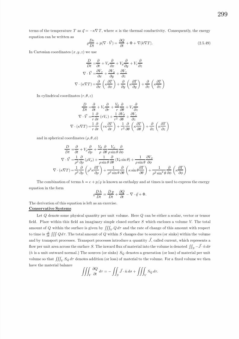
8/6/2019 Introduction to Tensor Calculus Continuum Mechanics - J. Heinbockel
http://slidepdf.com/reader/full/introduction-to-tensor-calculus-continuum-mechanics-j-heinbockel 305/372
29
terms of the temperature T as q = −κ∇ T , where κ is the thermal conductivity. Consequently, the energy
equation can be written as
De
Dt+ p(∇ · V ) =
∂Q
∂t+ Φ + ∇(k∇T ). (2.5.49)
In Cartesian coordinates (x, y, z) we use
DDt
=∂ ∂t
+ V x∂
∂x+ V y
∂ ∂y
+ V z∂
∂z
∇ · V =∂V x∂x
+∂V y∂y
+∂V z∂z
∇ · (κ∇T ) =∂
∂x
κ
∂T
∂x
+
∂
∂y
κ
∂T
∂y
+
∂
∂z
κ
∂T
∂z
In cylindrical coordinates (r,θ,z)
D
Dt=
∂
∂t+ V r
∂
∂r+
V θr
∂
∂θ+ V z
∂
∂z
∇ · V =
1
r
∂
∂r(rV
r) +
1
r2
∂V θ
∂θ+
∂V z
∂z
∇ · (κ∇T ) =1
r
∂
∂r
rκ
∂T
∂r
+
1
r2∂
∂θ
κ
∂T
∂θ
+
∂
∂z
κ
∂T
∂z
and in spherical coordinates (ρ,θ,φ)
D
Dt=
∂
∂t+ V ρ
∂
∂ρ+
V θρ
∂
∂θ
V φρ sin θ
∂
∂φ
∇ · V =1
ρ2∂
∂ρ(ρV ρ) +
1
ρ sin θ
∂
∂θ(V θ sin θ) +
1
ρ sin θ
∂V φ∂φ
∇ · (κ∇T ) =1
ρ2∂
∂ρ
ρ2κ
∂T
∂ρ
+
1
ρ2 sin θ
∂
∂θ
κ sin θ
∂T
∂θ
+
1
ρ2 sin2 θ
∂
∂φ
κ
∂T
∂φ
The combination of terms h = e + p/ is known as enthalpy and at times is used to express the energy
equation in the form
D h
Dt=
D p
Dt+
∂Q
∂t− ∇ · q + Φ.
The derivation of this equation is left as an exercise.
Conservative Systems
Let Q denote some physical quantity per unit volume. Here Q can be either a scalar, vector or tensor
field. Place within this field an imaginary simple closed surface S which encloses a volume V. The total
amount of Q within the surface is given by
V Q dτ and the rate of change of this amount with respect
to time is ∂ ∂t Qdτ. The total amount of Q within S changes due to sources (or sinks) within the volume
and by transport processes. Transport processes introduce a quantity J, called current, which represents a
flow per unit area across the surface S. The inward flux of material into the volume is denoted
S− J · n dσ
(n is a unit outward normal.) The sources (or sinks) S Q denotes a generation (or loss) of material per unit
volume so that
V S Q dτ denotes addition (or loss) of material to the volume. For a fixed volume we then
have the material balance V
∂Q
∂tdτ = −
S
J · n dσ +
V
S Q dτ.

8/6/2019 Introduction to Tensor Calculus Continuum Mechanics - J. Heinbockel
http://slidepdf.com/reader/full/introduction-to-tensor-calculus-continuum-mechanics-j-heinbockel 306/372
300
Using the divergence theorem of Gauss one can derive the general conservation law
∂Q
∂t+ ∇ · J = S Q (2.5.50)
The continuity equation and energy equations are examples of a scalar conservation law in the special case
where S Q
= 0. In Cartesian coordinates, we can represent the continuity equation by letting
Q = and J = V = (V x e1 + V y e2 + V z e3) (2.5.51)
The energy equation conservation law is represented by selecting Q = et and neglecting the rate of internal
heat energy we let
J =
(et + p)v1 −
3i=1
viτ xi + qx
e1+
(et + p)v2 −3i=1
viτ yi + qy
e2+
(et + p)v3 −3i=1
viτ zi + qz e3.
(2.5.52)
In a general orthogonal system of coordinates (x1, x2, x3) the equation (2.5.50) is written
∂
∂t((h1h2h3Q)) +
∂
∂x1((h2h3J 1)) +
∂
∂x2((h1h3J 2)) +
∂
∂x3((h1h2J 3)) = 0,
where h1, h2, h3 are scale factors obtained from the transformation equations to the general orthogonal
coordinates.
The momentum equations are examples of a vector conservation law having the form
∂a
∂t+ ∇ · (T ) = b (2.5.53)
where a is a vector and T is a second order symmetric tensor T =
3k=1
3j=1
T jk ej ek. In Cartesian coordinates
we let a = (V x e1 + V y e2 + V z e3) and T ij = vivj + pδij − τ ij . In general coordinates (x1, x2, x3) the
momentum equations result by selecting a = V and T ij = vivj + pδij − τ ij. In a general orthogonal system
the conservation law (2.5.53) has the general form
∂
∂t((h1h2h3a)) +
∂
∂x1
(h2h3T · e1)
+
∂
∂x2
(h1h3T · e2)
+
∂
∂x3
(h1h2T · e3)
= b. (2.5.54)
Neglecting body forces and internal heat production, the continuity, momentum and energy equations
can be expressed in the strong conservative form
∂U
∂t+
∂E
∂x+
∂F
∂y+
∂G
∂z= 0 (2.5.55)
where
U =
ρ
ρV xρV yρV zet
(2.5.56)

8/6/2019 Introduction to Tensor Calculus Continuum Mechanics - J. Heinbockel
http://slidepdf.com/reader/full/introduction-to-tensor-calculus-continuum-mechanics-j-heinbockel 307/372
30
E =
ρV x
ρV 2x + p − τ xxρV xV y − τ xyρV xV z − τ xz
(et + p)V x − V xτ xx − V yτ xy − V zτ xz + qx
(2.5.57)
F =
ρV y
ρV xV y − τ xyρV 2y + p − τ yy
ρV yV z − τ yz(et + p)V y − V xτ yx − V yτ yy − V zτ yz + qy
(2.5.58)
G =
ρV z
ρV xV z − τ xzρV yV z − τ yz
ρV 2z + p − τ zz(et + p)V z − V xτ zx − V yτ zy − V zτ zz + qz
(2.5.59)
where the shear stresses are τ ij = µ∗(V i,j + V j,i) + δijλ∗V k,k for i,j,k = 1, 2, 3.
Computational Coordinates
To transform the conservative system (2.5.55) from a physical (x, y, z) domain to a computational (ξ, η, ζ )domain requires that a general change of variables take place. Consider the following general transformation
of the independent variables
ξ = ξ(x, y, z) η = η(x, y, z) ζ = ζ (x, y, z) (2.5.60)
with Jacobian different from zero. The chain rule for changing variables in equation (2.5.55) requires the
operators∂ ( )
∂x=
∂ ( )
∂ξξx +
∂ ( )
∂ηηx +
∂ ( )
∂ζ ζ x
∂ ( )
∂y =
∂ ( )
∂ξ ξy +
∂ ( )
∂η ηy +
∂ ( )
∂ζ ζ y
∂ ( )
∂z=
∂ ( )
∂ξξz +
∂ ( )
∂ηηz +
∂ ( )
∂ζ ζ z
(2.5.61)
The partial derivatives in these equations occur in the differential expressions
dξ =ξx dx + ξy dy + ξz dz
dη =ηx dx + ηy dy + ηz dz
dζ =ζ x dx + ζ y dy + ζ z dz
or
dξdηdζ
=
ξx ξy ξzηx ηy ηzζ x ζ y ζ z
dxdydz
(2.5.62)
In a similar mannaer from the inverse transformation equations
x = x(ξ, η, ζ ) y = y(ξ, η, ζ ) z = z(ξ, η, ζ ) (2.5.63)
we can write the differentials
dx =xξ dξ + xη dη + xζ dζ
dy =yξ dξ + yη dη + yζ dζ
dz =zξ dξ + zζ dζ + zζ dζ
or
dxdydz
=
xξ xη xζyξ yη yζzξ zη zζ
dξdηdζ
(2.5.64)

8/6/2019 Introduction to Tensor Calculus Continuum Mechanics - J. Heinbockel
http://slidepdf.com/reader/full/introduction-to-tensor-calculus-continuum-mechanics-j-heinbockel 308/372
302
The transformations (2.5.62) and (2.5.64) are inverses of each other and so we can write ξx ξy ξzηx ηy ηzζ x ζ y ζ z
=
xξ xη xζyξ yη yζzξ zη zζ
−1
=J yηzζ−
yζzη−
(xηzζ−
xζzη) xηyζ−
xζyη−(yξzζ − yζzξ) xξzζ − xζzξ −(xξyζ − xζyξ)
yξzη − yηzξ −(xξzη − xηzξ) xξyη − xηyξ
(2.5.65)
By comparing like elements in equation (2.5.65) we obtain the relations
ξx =J (yηzζ − yζzη)
ξy = − J (xηzζ − xζzη)
ξz =J (xηyζ − xζyη)
ηx = − J (yξzζ − yζzξ)
ηy =J (xξzζ − zζzξ)
ηz = − J (xξyζ − xζyξ)
ζ x =J (yξzη − yηzξ)
ζ y = − J (xξzη − xηzξ)
ζ z =J (xξyη − xηyξ)
(2.5.66)
The equations (2.5.55) can now be written in terms of the new variables (ξ, η, ζ ) as
∂U
∂t +∂E
∂ξ ξx +∂E
∂η ηx +∂E
∂ζ ζ x +∂F
∂ξ ξy +∂F
∂η ηy +∂F
∂ζ ζ y +∂G
∂ξ ξz +∂G
∂η ηz +∂G
∂ζ ζ z = 0 (2.5.67)
Now divide each term by the Jacobian J and write the equation (2.5.67) in the form
∂
∂t
U
J
+
∂
∂ξ
Eξx + F ξy + Gξz
J
+
∂
∂η
Eηx + F ηy + Gηz
J
+
∂
∂ζ
Eζ x + F ζ y + Gζ z
J
−E
∂
∂ξ ξx
J +∂
∂η ηx
J +∂
∂ζ ζ x
J − F
∂
∂ξ
ξyJ
+
∂
∂η
ηyJ
+
∂
∂ζ
ζ yJ
− G
∂
∂ξ
ξzJ
+
∂
∂η
ηzJ
+
∂
∂ζ
ζ zJ
= 0
(2.5.68)
Using the relations given in equation (2.5.66) one can show that the curly bracketed terms above are all zero
and so the transformed equations (2.5.55) can also be written in the conservative form
∂ U
∂t+
∂ E
∂ξ+
∂ F
∂η+
∂ G∂ζ
= 0 (2.5.69)
where U =U
J E =Eξx + F ξy + Gξz
J F =Eηx + F ηy + Gηz
J G =Eζ x + F ζ y + Gζ z
J
(2.5.70)

8/6/2019 Introduction to Tensor Calculus Continuum Mechanics - J. Heinbockel
http://slidepdf.com/reader/full/introduction-to-tensor-calculus-continuum-mechanics-j-heinbockel 309/372
30
Fourier law of heat conduction
The Fourier law of heat conduction can be written qi = −κT ,i for isotropic material and qi = −κijT ,j
for anisotropic material. The Prandtl number is a nondimensional constant defined as P r =cpµ
∗
κ so that
the heat flow terms can be represented in Cartesian coordinates as
qx = −c pµ∗
P r
∂T
∂x qy = −c pµ∗
P r
∂T
∂y qz = −c pµ∗
P r
∂T
∂z
Now one can employ the equation of state relations P = e(γ − 1), c p = γRγ−1 , c pT = γRT
γ−1 and write the
above equations in the alternate forms
qx = − µ∗
P r(γ − 1)
∂
∂x
γP
qy = − µ∗
P r(γ − 1)
∂
∂y
γP
qz = − µ∗
P r(γ − 1)
∂
∂z
γP
The speed of sound is given by a =
γP
=
γRT and so one can substitute a2 in place of the ratioγP
in the above equations.
Equilibrium and Nonequilibrium ThermodynamicsHigh temperature gas flows require special considerations. In particular, the specific heat for monotonic
and diatomic gases are different and are in general a function of temperature. The energy of a gas can be
written as e = et + er + ev + ee + en where et represents translational energy, er is rotational energy, ev is
vibrational energy, ee is electronic energy, and en is nuclear energy. The gases follow a Boltzmann distribution
for each degree of freedom and consequently at very high temperatures the rotational, translational and
vibrational degrees of freedom can each have their own temperature. Under these conditions the gas is said
to be in a state of nonequilibrium. In such a situation one needs additional energy equations. The energy
equation developed in these notes is for equilibrium thermodynamics where the rotational, translational and
vibrational temperatures are the same.
Equation of state
It is assumed that an equation of state such as the universal gas law or perfect gas law pV = nRT
holds which relates pressure p [N/m2], volume V [m3], amount of gas n [mol],and temperature T [K ] where
R [J/mol − K ] is the universal molar gas constant. If the ideal gas law is represented in the form p = RT
where [Kg/m3] is the gas density, then the universal gas constant must be expressed in units of [ J/Kg−K ]
(See Appendix A). Many gases deviate from this ideal behavior. In order to account for the intermolecular
forces associated with high density gases, an empirical equation of state of the form
p = ρRT +M 1
n=1β nρn+r1 + e−γ1ρ−γ2ρ
2
M 2
n=1cnρn+r2
involving constants M 1, M 2, β n, cn, r1, r2, γ 1, γ 2 is often used. For a perfect gas the relations
e = cvT γ =c pcv
cv =R
γ − 1c p =
γR
γ − 1h = c pT
hold, where R is the universal gas constant, cv is the specific heat at constant volume, c p is the specific
heat at constant pressure, γ is the ratio of specific heats and h is the enthalpy. For cv and c p constants the
relations p = (γ − 1)e and RT = (γ − 1)e can be verified.

8/6/2019 Introduction to Tensor Calculus Continuum Mechanics - J. Heinbockel
http://slidepdf.com/reader/full/introduction-to-tensor-calculus-continuum-mechanics-j-heinbockel 310/372
304
EXAMPLE 2.5-1. (One-dimensional fluid flow)
Construct an x-axis running along the center line of a long cylinder with cross sectional area A. Consider
the motion of a gas driven by a piston and moving with velocity v1 = u in the x-direction. From an Eulerian
point of view we imagine a control volume fixed within the cylinder and assume zero body forces. We require
the following equations be satisfied.
Conservation of mass ∂∂t
+ div( V ) = 0 which in one-dimension reduces to ∂∂t
+ ∂ ∂x
(u) = 0.
Conservation of momentum, equation (2.5.28) reduces to∂
∂t(u) +
∂
∂x
u2
+
∂p
∂x= 0.
Conservation of energy, equation (2.5.48) in the absence of heat flow and internal heat production,
becomes in one dimension
∂e
∂t+ u
∂e
∂x
+ p
∂u
∂x= 0. Using the conservation of mass relation this
equation can be written in the form∂
∂t(e) +
∂
∂x(eu) + p
∂u
∂x= 0.
In contrast, from a Lagrangian point of view we let the control volume move with the flow and consider
advection terms. This gives the following three equations which can then be compared with the above
Eulerian equations of motion.
Conservation of mass
d
dt (J ) = 0 which in one-dimension is equivalent to
D
Dt +
∂u
∂x = 0.
Conservation of momentum, equation (2.5.25) in one-dimension Du
Dt+
∂p
∂x= 0.
Conservation of energy, equation (2.5.48) in one-dimension De
Dt+ p
∂u
∂x= 0. In the above equations
D( )Dt = ∂
∂t ( ) + u ∂ ∂x ( ). The Lagrangian viewpoint gives three equations in the three unknowns ρ,u,e.
In both the Eulerian and Lagrangian equations the pressure p represents the total pressure p = pg + pv
where pg is the gas pressure and pv is the viscous pressure which causes loss of kinetic energy. The gas pressure
is a function of , e and is determined from the ideal gas law pg = RT = (c p − cv)T = (cpcv
− 1)cvT or
pg = (γ − 1)e. Some kind of assumption is usually made to represent the viscous pressure pv as a function
of e, u. The above equations are then subjected to boundary and initial conditions and are usually solved
numerically.
Entropy inequality
Energy transfer is not always reversible. Many energy transfer processes are irreversible. The second
law of thermodynamics allows energy transfer to be reversible only in special circumstances. In general,
the second law of thermodynamics can be written as an entropy inequality, known as the Clausius-Duhem
inequality. This inequality states that the time rate of change of the total entropy is greater than or equal to
the total entropy change occurring across the surface and within the body of a control volume. The Clausius-
Duhem inequality places restrictions on the constitutive equations. This inequality can be expressed in the
form D
Dt
V
sdτ Rate of entropy increase
≥ S
sini dS + V
ρbdτ +n
α=1
B(α) Entropy input rate into control volume
where s is the specific entropy density, si is an entropy flux, b is an entropy source and B(α) are isolated
entropy sources. Irreversible processes are characterized by the use of the inequality sign while for reversible
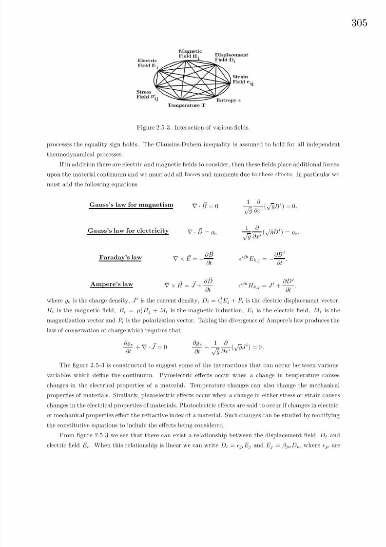
8/6/2019 Introduction to Tensor Calculus Continuum Mechanics - J. Heinbockel
http://slidepdf.com/reader/full/introduction-to-tensor-calculus-continuum-mechanics-j-heinbockel 311/372
30
Figure 2.5-3. Interaction of various fields.
processes the equality sign holds. The Clausius-Duhem inequality is assumed to hold for all independent
thermodynamical processes.
If in addition there are electric and magnetic fields to consider, then these fields place additional forces
upon the material continuum and we must add all forces and moments due to these effects. In particular we
must add the following equations
Gauss’s law for magnetism ∇ · B = 01√
g
∂
∂xi(√
gB i) = 0.
Gauss’s law for electricity ∇ · D = e1√
g
∂
∂xi(√
gDi) = e.
Faraday’s law ∇ × E = −∂ B
∂tijkE k,j = −∂B i
∂t.
Ampere’s law ∇ × H =
J +
∂ D
∂t ijk
H k,j = J i
+
∂Di
∂t .
where e is the charge density, J i is the current density, Di = jiE j + P i is the electric displacement vector,
H i is the magnetic field, Bi = µjiH j + M i is the magnetic induction, E i is the electric field, M i is the
magnetization vector and P i is the polarization vector. Taking the divergence of Ampere’s law produces the
law of conservation of charge which requires that
∂e∂t
+ ∇ · J = 0∂e∂t
+1√
g
∂
∂xi(√
gJ i) = 0.
The figure 2.5-3 is constructed to suggest some of the interactions that can occur between various
variables which define the continuum. Pyroelectric effects occur when a change in temperature causes
changes in the electrical properties of a material. Temperature changes can also change the mechanical
properties of materials. Similarly, piezoelectric effects occur when a change in either stress or strain causes
changes in the electrical properties of materials. Photoelectric effects are said to occur if changes in electric
or mechanical properties effect the refractive index of a material. Such changes can be studied by modifying
the constitutive equations to include the effects being considered.
From figure 2.5-3 we see that there can exist a relationship between the displacement field Di and
electric field E i. When this relationship is linear we can write Di = jiE j and E j = β jnDn, where ji are
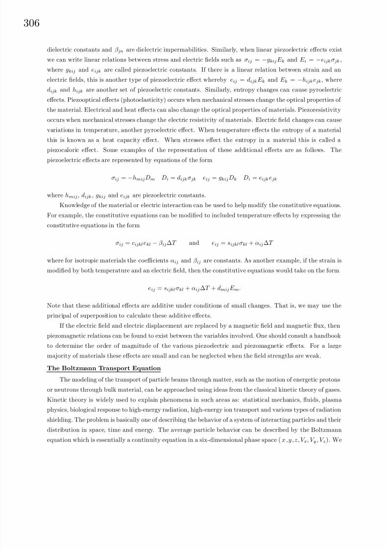
8/6/2019 Introduction to Tensor Calculus Continuum Mechanics - J. Heinbockel
http://slidepdf.com/reader/full/introduction-to-tensor-calculus-continuum-mechanics-j-heinbockel 312/372
306
dielectric constants and β jn are dielectric impermabilities. Similarly, when linear piezoelectric effects exist
we can write linear relations between stress and electric fields such as σij = −gkijE k and E i = −eijkσjk ,
where gkij and eijk are called piezoelectric constants. If there is a linear relation between strain and an
electric fields, this is another type of piezoelectric effect whereby eij = dijkE k and E k = −hijkejk , where
dijk and hijk are another set of piezoelectric constants. Similarly, entropy changes can cause pyroelectric
effects. Piezooptical effects (photoelasticity) occurs when mechanical stresses change the optical properties of
the material. Electrical and heat effects can also change the optical properties of materials. Piezoresistivity
occurs when mechanical stresses change the electric resistivity of materials. Electric field changes can cause
variations in temperature, another pyroelectric effect. When temperature effects the entropy of a material
this is known as a heat capacity effect. When stresses effect the entropy in a material this is called a
piezocaloric effect. Some examples of the representation of these additional effects are as follows. The
piezoelectric effects are represented by equations of the form
σij = −hmijDm Di = dijkσjk eij = gkijDk Di = eijkejk
where hmij, dijk , gkij and eijk are piezoelectric constants.
Knowledge of the material or electric interaction can be used to help modify the constitutive equations.
For example, the constitutive equations can be modified to included temperature effects by expressing the
constitutive equations in the form
σij = cijklekl − β ij∆T and eij = sijklσkl + αij∆T
where for isotropic materials the coefficients αij and β ij are constants. As another example, if the strain is
modified by both temperature and an electric field, then the constitutive equations would take on the form
eij = sijklσkl + αij∆T + dmijE m.
Note that these additional effects are additive under conditions of small changes. That is, we may use the
principal of superposition to calculate these additive effects.
If the electric field and electric displacement are replaced by a magnetic field and magnetic flux, then
piezomagnetic relations can be found to exist between the variables involved. One should consult a handbook
to determine the order of magnitude of the various piezoelectric and piezomagnetic effects. For a large
majority of materials these effects are small and can be neglected when the field strengths are weak.
The Boltzmann Transport Equation
The modeling of the transport of particle beams through matter, such as the motion of energetic protons
or neutrons through bulk material, can be approached using ideas from the classical kinetic theory of gases.
Kinetic theory is widely used to explain phenomena in such areas as: statistical mechanics, fluids, plasma
physics, biological response to high-energy radiation, high-energy ion transport and various types of radiation
shielding. The problem is basically one of describing the behavior of a system of interacting particles and their
distribution in space, time and energy. The average particle behavior can be described by the Boltzmann
equation which is essentially a continuity equation in a six-dimensional phase space ( x, y, z, V x, V y , V z). We

8/6/2019 Introduction to Tensor Calculus Continuum Mechanics - J. Heinbockel
http://slidepdf.com/reader/full/introduction-to-tensor-calculus-continuum-mechanics-j-heinbockel 313/372
30
will be interested in examining how the particles in a volume element of phase space change with time. We
introduce the following notation:
(i) r the position vector of a typical particle of phase space and dτ = dxdydz the corresponding spatial
volume element at this position.
(ii) V the velocity vector associated with a typical particle of phase space and dτ v = dV xdV ydV z the
corresponding velocity volume element.
(iii) Ω a unit vector in the direction of the velocity V = v Ω.
(iv) E = 12mv2 kinetic energy of particle.
(v) d Ω is a solid angle about the direction Ω and dτ dE d Ω is a volume element of phase space involving the
solid angle about the direction Ω.
(vi) n = n(r, E, Ω, t) the number of particles in phase space per unit volume at position r per unit velocity
at position V per unit energy in the solid angle d Ω at time t and N = N (r, E, Ω, t) = vn(r, E, Ω, t)
the number of particles per unit volume per unit energy in the solid angle d Ω at time t. The quantity
N (r, E, Ω, t)dτ dE d Ω represents the number of particles in a volume element around the position r with
energy between E and E + dE having direction Ω in the solid angle d
Ω at time t.
(vii) φ(r, E, Ω, t) = vN (r, E, Ω, t) is the particle flux (number of particles/cm2 − Mev − sec).
(viii) Σ(E → E, Ω → Ω) a scattering cross-section which represents the fraction of particles with energy E
and direction Ω that scatter into the energy range between E and E + dE having direction Ω in the
solid angle d Ω per particle flux.
(ix) Σs(E, r) fractional number of particles scattered out of volume element of phase space per unit volume
per flux.
(x) Σa(E, r) fractional number of particles absorbed in a unit volume of phase space per unit volume per
flux.
Consider a particle at time t having a position r in phase space as illustrated in the figure 2.5-4. This
particle has a velocity V in a direction Ω and has an energy E . In terms of dτ = dxdy dz, Ω and E an
element of volume of phase space can be denoted dτdEd Ω, where d Ω = d Ω(θ, ψ) = sin θdθdψ is a solid angle
about the direction Ω.
The Boltzmann transport equation represents the rate of change of particle density in a volume element
dτ dE d Ω of phase space and is written
d
dtN (r, E, Ω, t) dτ dE d Ω = DC N (r, E, Ω, t) (2.5.71)
where DC is a collision operator representing gains and losses of particles to the volume element of phase
space due to scattering and absorption processes. The gains to the volume element are due to any sources
S (r, E, Ω, t) per unit volume of phase space, with units of number of particles/sec per volume of phase space,
together with any scattering of particles into the volume element of phase space. That is particles entering
the volume element of phase space with energy E , which experience a collision, leave with some energy
E − ∆E and thus will be lost from our volume element. Particles entering with energies E > E may,

8/6/2019 Introduction to Tensor Calculus Continuum Mechanics - J. Heinbockel
http://slidepdf.com/reader/full/introduction-to-tensor-calculus-continuum-mechanics-j-heinbockel 314/372
308
Figure 2.5-4. Volume element and solid angle about position r.
depending upon the cross-sections, exit with energy E − ∆E = E and thus will contribute a gain to the
volume element. In terms of the flux φ the gains due to scattering into the volume element are denoted by d Ω
dE Σ(E → E, Ω → Ω)φ(r, E , Ω, t) dτ dE d Ω
and represents the particles at position r experiencing a scattering collision with a particle of energy E and
direction Ω which causes the particle to end up with energy between E and E + dE and direction Ω in d Ω.
The summations are over all possible initial energies.
In terms of φ the losses are due to those particles leaving the volume element because of scattering and
are
Σs(E, r)φ(r, E, Ω, t)dτ dE d
Ω.
The particles which are lost due to absorption processes are
Σa(E, r)φ(r, E, Ω, t) dτ dE d Ω.
The total change to the number of particles in an element of phase space per unit of time is obtained by
summing all gains and losses. This total change is
dN
dtdτ dE dΩ =
d Ω
dE Σ(E → E, Ω → Ω)φ(r, E , Ω, t) dτ dE d Ω
− Σs(E, r)φ(r, E, Ω, t)dτ dE dΩ
− Σa(E, r)φ(r, E, Ω, t) dτ dE d Ω+ S (r, E, Ω, t)dτ dE d Ω.
(2.5.72)
The rate of change dN dt on the left-hand side of equation (2.5.72) expands to
dN
dt=
∂N
∂t+
∂N
∂x
dx
dt+
∂N
∂y
dy
dt+
∂N
∂z
dz
dt
+∂N
∂V x
dV xdt
+∂N
∂V y
dV ydt
+∂N
∂V z
dV zdt

8/6/2019 Introduction to Tensor Calculus Continuum Mechanics - J. Heinbockel
http://slidepdf.com/reader/full/introduction-to-tensor-calculus-continuum-mechanics-j-heinbockel 315/372
30
which can be written asdN
dt=
∂N
∂t+ V · ∇rN +
F
m· ∇ V N (2.5.73)
where d V dt =
F m represents any forces acting upon the particles. The Boltzmann equation can then be
expressed as
∂N ∂t
+ V · ∇rN + F m
· ∇ V N = Gains − Losses. (2.5.74)
If the right-hand side of the equation (2.5.74) is zero, the equation is known as the Liouville equation. In
the special case where the velocities are constant and do not change with time the above equation (2.5.74)
can be written in terms of the flux φ and has the form1
v
∂
∂t+ Ω · ∇r + Σs(E, r) + Σa(E, r)
φ(r, E, Ω, t) = DC φ (2.5.75)
where
DC φ =
d Ω
dE Σ(E → E, Ω → Ω)φ(r, E , Ω, t) + S (r, E, Ω, t).
The above equation represents the Boltzmann transport equation in the case where all the particles are
the same. In the case of atomic collisions of particles one must take into consideration the generation of
secondary particles resulting from the collisions.
Let there be a number of particles of type j in a volume element of phase space. For example j = p
(protons) and j = n (neutrons). We consider steady state conditions and define the quantities
(i) φj(r, E, Ω) as the flux of the particles of type j.
(ii) σjk( Ω, Ω, E , E ) the collision cross-section representing processes where particles of type k moving in
direction Ω with energy E produce a type j particle moving in the direction Ω with energy E .
(iii) σj(E ) = Σs(E, r) + Σa(E, r) the cross-section for type j particles.
The steady state form of the equation (2.5.64) can then be written as
Ω · ∇φj(r, E, Ω)+σj(E )φj(r, E, Ω)
=k
σjk( Ω, Ω, E , E )φk(r, E , Ω)d ΩdE
(2.5.76)
where the summation is over all particles k = j.
The Boltzmann transport equation can be represented in many different forms. These various forms
are dependent upon the assumptions made during the derivation, the type of particles, and collision cross-
sections. In general the collision cross-sections are dependent upon three components.
(1) Elastic collisions. Here the nucleus is not excited by the collision but energy is transferred by projectile
recoil.(2) Inelastic collisions. Here some particles are raised to a higher energy state but the excitation energy is
not sufficient to produce any particle emissions due to the collision.
(3) Non-elastic collisions. Here the nucleus is left in an excited state due to the collision processes and
some of its nucleons (protons or neutrons) are ejected. The remaining nucleons interact to form a stable
structure and usually produce a distribution of low energy particles which is isotropic in character.

8/6/2019 Introduction to Tensor Calculus Continuum Mechanics - J. Heinbockel
http://slidepdf.com/reader/full/introduction-to-tensor-calculus-continuum-mechanics-j-heinbockel 316/372
310
Various assumptions can be made concerning the particle flux. The resulting form of Boltzmann’s
equation must be modified to reflect these additional assumptions. As an example, we consider modifications
to Boltzmann’s equation in order to describe the motion of a massive ion moving into a region filled with a
homogeneous material. Here it is assumed that the mean-free path for nuclear collisions is large in comparison
with the mean-free path for ion interaction with electrons. In addition, the following assumptions are made
(i) All collision interactions are non-elastic.
(ii) The secondary particles produced have the same direction as the original particle. This is called the
straight-ahead approximation.
(iii) Secondary particles never have kinetic energies greater than the original projectile that produced them.
(iv) A charged particle will eventually transfer all of its kinetic energy and stop in the media. This stopping
distance is called the range of the projectile. The stopping power S j(E ) = dEdx represents the energy
loss per unit length traveled in the media and determines the range by the relationdRj
dE = 1Sj(E)
or
Rj(E ) = E0
dE
Sj(E). Using the above assumptions Wilson, et.al.1 show that the steady state linearized
Boltzmann equation for homogeneous materials takes on the form
Ω · ∇φj(r, E, Ω) − 1Aj
∂ ∂E
(S j(E )φj(r, E, Ω)) + σj(E )φj(r, E, Ω)
=k=j
dE d Ω σjk( Ω, Ω, E , E )φk(r, E , Ω)
(2.5.77)
where Aj is the atomic mass of the ion of type j and φj(r, E, Ω) is the flux of ions of type j moving in
the direction Ω with energy E .
Observe that in most cases the left-hand side of the Boltzmann equation represents the time rate of
change of a distribution type function in a phase space while the right-hand side of the Boltzmann equation
represents the time rate of change of this distribution function within a volume element of phase space due
to scattering and absorption collision processes.
Boltzmann Equation for gases
Consider the Boltzmann equation in terms of a particle distribution function f (r, V , t) which can be
written as ∂
∂t+ V · ∇r +
F
m· ∇ V
f (r, V , t) = DC f (r, V , t) (2.5.78)
for a single species of gas particles where there is only scattering and no absorption of the particles. An
element of volume in phase space (x, y, z, V x, V y, V z) can be thought of as a volume element dτ = dxdydz
for the spatial elements together with a volume element dτ v = dV xdV ydV z for the velocity elements. These
elements are centered at position r and velocity V at time t. In phase space a constant velocity V 1 can be
thought of as a sphere since V 21 = V 2x + V 2y + V 2z . The phase space volume element dτdτ v changes with time
since the position r and velocity V change with time. The position vector r changes because of velocity
1John W. Wilson, Lawrence W. Townsend, Walter Schimmerling, Govind S. Khandelwal, Ferdous Kahn,
John E. Nealy, Francis A. Cucinotta, Lisa C. Simonsen, Judy L. Shinn, and John W. Norbury, Transport
Methods and Interactions for Space Radiations, NASA Reference Publication 1257, December 1991.

8/6/2019 Introduction to Tensor Calculus Continuum Mechanics - J. Heinbockel
http://slidepdf.com/reader/full/introduction-to-tensor-calculus-continuum-mechanics-j-heinbockel 317/372

8/6/2019 Introduction to Tensor Calculus Continuum Mechanics - J. Heinbockel
http://slidepdf.com/reader/full/introduction-to-tensor-calculus-continuum-mechanics-j-heinbockel 318/372
312
• The particle density per unit volume
n = n(r, t) =
dτ V f (r, V , t) =
+∞ −∞
f (r, V , t)dV xdV ydV z (2.5.84)
where ρ = nm is the mass density.• The mean velocity
V 1 = V =1
n
+∞ −∞
V 1f (r, V 1, t)dV 1xdV 1ydV 1z
For any quantity Q = Q( V 1) define the barred quantity
Q = Q(r, t) =1
n(r, t)
Q( V )f (r, V , t) dτ V =
1
n
+∞ −∞
Q( V )f (r, V , t)dV xdV ydV z . (2.5.85)
Further, assume that
F
m is independent of V , then the moment of equation (2.5.83) produces the result
∂
∂t
nφ
+3i=1
∂
∂xi
nV 1iφ− n
3i=1
F im
∂φ
∂V 1i= 0 (2.5.86)
known as the Maxwell transfer equation. The first term in equation (2.5.86) follows from the integrals ∂f (r, V 1, t)
∂tφ( V 1)dτ V 1 =
∂
∂t
f (r, V 1, t)φ( V 1) dτ V 1 =
∂
∂t(nφ) (2.5.87)
where differentiation and integration have been interchanged. The second term in equation (2.5.86) follows
from the integral V 1∇rf φ( V 1)dτ V 1 = 3i=1
V 1i ∂f ∂xi
φ dτ V 1
=
3i=1
∂
∂xi
V 1iφf dτ V 1
=3i=1
∂
∂xi
nV 1iφ
.
(2.5.88)
The third term in equation (2.5.86) is obtained from the following integral where integration by parts is
employed
F
m∇ V 1
fφdτ V 1 = 3
i=1 F i
m
∂f
∂V 1iφ dτ V 1
=
+∞ −∞
3i=1
φ
F im
∂f
∂V 1i
dV 1xdV 1ydV 1y
= −
∂
∂V 1i
F im
φ
f dτ V 1
= −n∂
∂V 1i
F im
φ
= −F i
m
∂φ
∂V 1i
(2.5.89)
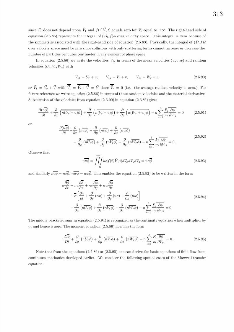
8/6/2019 Introduction to Tensor Calculus Continuum Mechanics - J. Heinbockel
http://slidepdf.com/reader/full/introduction-to-tensor-calculus-continuum-mechanics-j-heinbockel 319/372
31
since F i does not depend upon V 1 and f (r, V , t) equals zero for V i equal to ±∞. The right-hand side of
equation (2.5.86) represents the integral of (DC f )φ over velocity space. This integral is zero because of
the symmetries associated with the right-hand side of equation (2.5.83). Physically, the integral of (Dcf )φ
over velocity space must be zero since collisions with only scattering terms cannot increase or decrease the
number of particles per cubic centimeter in any element of phase space.
In equation (2.5.86) we write the velocities V 1i in terms of the mean velocities (u, v, w) and random
velocities (U r, V r, W r) with
V 11 = U r + u, V 12 = V r + v, V 13 = W r + w (2.5.90)
or V 1 = V r + V with V 1 = V r + V = V since V r = 0 (i.e. the average random velocity is zero.) For
future reference we write equation (2.5.86) in terms of these random velocities and the material derivative.
Substitution of the velocities from equation (2.5.90) in equation (2.5.86) gives
∂ (nφ)
∂t
+∂
∂x n(U r + u)φ +∂
∂y n(V r + v)φ+∂
∂z n(W r + w)φ−n
3
i=1F i
m
∂φ
∂V 1i= 0 (2.5.91)
or∂ (nφ)
∂t+
∂
∂x
nuφ
+
∂
∂y
nvφ
+
∂
∂z
nwφ
+
∂
∂x
nU rφ
+
∂
∂y
nV rφ
+
∂
∂z
nW rφ
− n3i=1
F im
∂φ
∂V 1i= 0.
(2.5.92)
Observe that
nuφ =
+∞ −∞
uφf (r, V , t)dV xdV ydV z = nuφ (2.5.93)
and similarly nvφ = nvφ, nwφ = nwφ. This enables the equation (2.5.92) to be written in the form
n∂φ
∂t+ nu
∂φ
∂x+ nv
∂φ
∂y+ nw
∂φ
∂z
+ φ
∂n
∂t+
∂
∂x(nu) +
∂
∂y(nv) +
∂
∂z(nw)
+
∂
∂x
nU rφ
+
∂
∂y
nV rφ
+
∂
∂z
nW rφ
− n3i=1
F im
∂φ
∂V 1i= 0.
(2.5.94)
The middle bracketed sum in equation (2.5.94) is recognized as the continuity equation when multiplied by
m and hence is zero. The moment equation (2.5.86) now has the form
nDφ
Dt+
∂
∂x
nU rφ
+
∂
∂y
nV rφ
+
∂
∂z
nW rφ
− n3i=1
F im
∂φ
∂V 1i= 0. (2.5.95)
Note that from the equations (2.5.86) or (2.5.95) one can derive the basic equations of fluid flow from
continuum mechanics developed earlier. We consider the following special cases of the Maxwell transfer
equation.
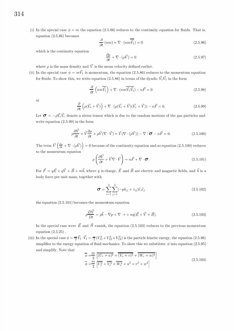
8/6/2019 Introduction to Tensor Calculus Continuum Mechanics - J. Heinbockel
http://slidepdf.com/reader/full/introduction-to-tensor-calculus-continuum-mechanics-j-heinbockel 320/372
314
(i) In the special case φ = m the equation (2.5.86) reduces to the continuity equation for fluids. That is,
equation (2.5.86) becomes∂
∂t(nm) + ∇ · (nm V 1) = 0 (2.5.96)
which is the continuity equation∂ρ
∂t + ∇ · (ρ V ) = 0 (2.5.97)
where ρ is the mass density and V is the mean velocity defined earlier.
(ii) In the special case φ = m V 1 is momentum, the equation (2.5.86) reduces to the momentum equation
for fluids. To show this, we write equation (2.5.86) in terms of the dyadic V 1 V 1 in the form
∂
∂t
nm V 1
+ ∇ · (nm V 1 V 1) − n F = 0 (2.5.98)
or∂
∂t
ρ( V r + V )
+ ∇ · (ρ( V r + V )( V r + V )) − n F = 0. (2.5.99)
Let σ = −ρ V r V r denote a stress tensor which is due to the random motions of the gas particles andwrite equation (2.5.99) in the form
ρ∂ V
∂t+ V
∂ρ
∂t+ ρ V (∇ · V ) + V (∇ · (ρ V )) − ∇ ·σ − n F = 0. (2.5.100)
The term V ∂ρ∂t + ∇ · (ρ V )
= 0 because of the continuity equation and so equation (2.5.100) reduces
to the momentum equation
ρ
∂ V
∂t+ V ∇ · V
= n F + ∇ ·σ. (2.5.101)
For F = q E + q V
× B + m b, where q is charge, E and B are electric and magnetic fields, and b is a
body force per unit mass, together with
σ =
3i=1
3j=1
(− pδij + τ ij) ei ej (2.5.102)
the equation (2.5.101) becomes the momentum equation
ρD V
Dt= ρ b − ∇ p + ∇ · τ + nq( E + V × B). (2.5.103)
In the special case were E and B vanish, the equation (2.5.103) reduces to the previous momentum
equation (2.5.25) .(iii) In the special case φ = m
2 V 1 · V 1 = m
2 (V 211 + V 212 + V 213) is the particle kinetic energy, the equation (2.5.86)
simplifies to the energy equation of fluid mechanics. To show this we substitute φ into equation (2.5.95)
and simplify. Note that
φ =m
2
(U r + u)2 + (V r + v)2 + (W r + w)2
φ =
m
2
U 2r + V 2r + W 2r + u2 + v2 + w2
(2.5.104)
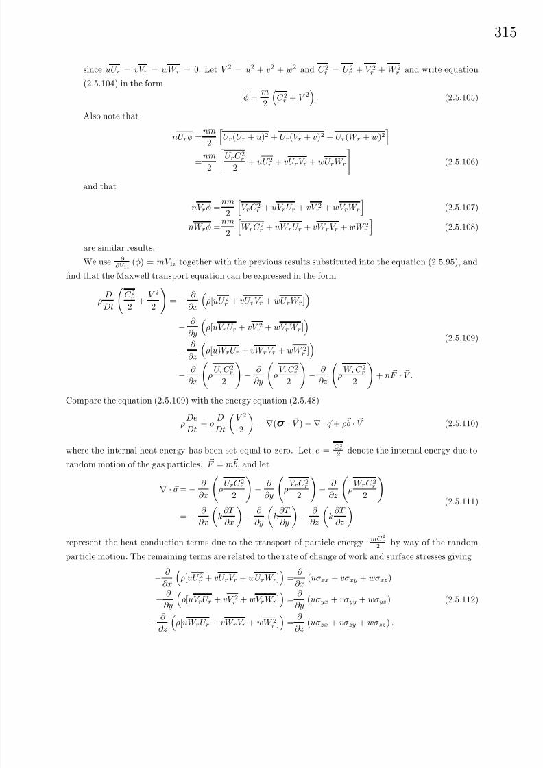
8/6/2019 Introduction to Tensor Calculus Continuum Mechanics - J. Heinbockel
http://slidepdf.com/reader/full/introduction-to-tensor-calculus-continuum-mechanics-j-heinbockel 321/372
31
since uU r = vV r = wW r = 0. Let V 2 = u2 + v2 + w2 and C 2r = U 2r + V 2r + W 2r and write equation
(2.5.104) in the form
φ =m
2
C 2r + V 2
. (2.5.105)
Also note that
nU rφ = nm2U r(U r + u)2 + U r(V r + v)2 + U r(W r + w)2
=nm
2
U rC 2r
2+ uU 2r + vU rV r + wU rW r
(2.5.106)
and that
nV rφ =nm
2
V rC 2r + uV rU r + vV 2r + wV rW r
(2.5.107)
nW rφ =nm
2
W rC 2r + uW rU r + vW rV r + wW 2r
(2.5.108)
are similar results.
We use ∂ ∂V 1
i
(φ) = mV 1i together with the previous results substituted into the equation (2.5.95), and
find that the Maxwell transport equation can be expressed in the form
ρD
Dt
C 2r2
+V 2
2
= − ∂
∂x
ρ[uU 2r + vU rV r + wU rW r]
− ∂
∂y
ρ[uV rU r + vV 2r + wV rW r]
− ∂
∂z
ρ[uW rU r + vW rV r + wW 2r ]
− ∂
∂x
ρ
U rC 2r2
− ∂
∂y
ρ
V rC 2r2
− ∂
∂z
ρ
W rC 2r2
+ n F · V .
(2.5.109)
Compare the equation (2.5.109) with the energy equation (2.5.48)
ρDe
Dt+ ρ
D
Dt
V 2
2
= ∇(σ · V ) − ∇ · q + ρ b · V (2.5.110)
where the internal heat energy has been set equal to zero. Let e =C 2r2 denote the internal energy due to
random motion of the gas particles, F = m b, and let
∇ · q = − ∂
∂x
ρ
U rC 2r2
− ∂
∂y
ρ
V rC 2r2
− ∂
∂z
ρ
W rC 2r2
= − ∂
∂x
k
∂T
∂x
− ∂
∂y
k
∂T
∂y
− ∂
∂z
k
∂T
∂z
(2.5.111)
represent the heat conduction terms due to the transport of particle energy mC 2
r
2 by way of the random
particle motion. The remaining terms are related to the rate of change of work and surface stresses giving
− ∂
∂x
ρ[uU 2r + vU rV r + wU rW r]
=
∂
∂x(uσxx + vσxy + wσxz)
− ∂
∂y
ρ[uV rU r + vV 2r + wV rW r]
=
∂
∂y(uσyx + vσyy + wσyz )
− ∂
∂z
ρ[uW rU r + vW rV r + wW 2r ]
=
∂
∂z(uσzx + vσzy + wσzz) .
(2.5.112)

8/6/2019 Introduction to Tensor Calculus Continuum Mechanics - J. Heinbockel
http://slidepdf.com/reader/full/introduction-to-tensor-calculus-continuum-mechanics-j-heinbockel 322/372
316
This gives the stress relations due to random particle motion
σxx = − ρU 2r
σxy = − ρU rV r
σxz =
−ρU rW r
σyx = − ρV rU r
σyy = − ρV 2r
σyz =
−ρV rW r
σzx = − ρW rU r
σzy = − ρW rV r
σzz =
−ρW 2r .
(2.5.113)
The Boltzmann equation is a basic macroscopic model used for the study of individual particle motion
where one takes into account the distribution of particles in both space, time and energy. The Boltzmann
equation for gases assumes only binary collisions as three-body or multi-body collisions are assumed to
rarely occur. Another assumption used in the development of the Boltzmann equation is that the actual
time of collision is thought to be small in comparison with the time between collisions. The basic problem
associated with the Boltzmann equation is to find a velocity distribution, subject to either boundary and/or
initial conditions, which describes a given gas flow.
The continuum equations involve trying to obtain the macroscopic variables of density, mean velocity,
stress, temperature and pressure which occur in the basic equations of continuum mechanics considered
earlier. Note that the moments of the Boltzmann equation, derived for gases, also produced these same
continuum equations and so they are valid for gases as well as liquids.
In certain situations one can assume that the gases approximate a Maxwellian distribution
f (r, V , t) ≈ n(r, t) m
2πkT
3/2exp
− m
2kT V · V
(2.5.114)
thereby enabling the calculation of the pressure tensor and temperature from statistical considerations.
In general, one can say that the Boltzmann integral-differential equation and the Maxwell transfer
equation are two important formulations in the kinetic theory of gases. The Maxwell transfer equation
depends upon some gas-particle property φ which is assumed to be a function of the gas-particle velocity.
The Boltzmann equation depends upon a gas-particle velocity distribution function f which depends upon
position r, velocity V and time t. These formulations represent two distinct and important viewpoints
considered in the kinetic theory of gases.

8/6/2019 Introduction to Tensor Calculus Continuum Mechanics - J. Heinbockel
http://slidepdf.com/reader/full/introduction-to-tensor-calculus-continuum-mechanics-j-heinbockel 323/372
31
EXERCISE 2.5
1. Let p = p(x, y, z), [dyne/cm2] denote the pressure at a point (x, y, z) in a fluid medium at rest
(hydrostatics), and let ∆V denote an element of fluid volume situated at this point as illustrated in the
figure 2.5-5.
Figure 2.5-5. Pressure acting on a volume element.
(a) Show that the force acting on the face ABCD is p(x, y, z)∆y∆z e1.
(b) Show that the force acting on the face EFGH is
− p(x + ∆x, y, z)∆y∆z e1 = − p(x, y, z) +∂p∂x
∆x +∂ 2 p∂x2
(∆x)2
2!+ · · ·∆y∆z e1.
(c) In part (b) neglect terms with powers of ∆x greater than or equal to 2 and show that the resultant force
in the x-direction is − ∂p
∂x∆x∆y∆z e1.
(d) What has been done in the x-direction can also be done in the y and z-directions. Show that the
resultant forces in these directions are − ∂p
∂y∆x∆y∆z e2 and − ∂p
∂z∆x∆y∆z e3. (e) Show that −∇ p =
−
∂p
∂xe1 +
∂p
∂ye2 +
∂p
∂ze3
is the force per unit volume acting at the point (x, y, z) of the fluid medium.
2. Follow the example of exercise 1 above but use cylindrical coordinates and find the force per unit volume
at a point (r,θ,z). Hint: An element of volume in cylindrical coordinates is given by ∆V = r∆r∆θ∆z. 3. Follow the example of exercise 1 above but use spherical coordinates and find the force per unit volume
at a point (ρ,θ,φ). Hint: An element of volume in spherical coordinates is ∆V = ρ2 sin θ∆ρ∆θ∆φ.
4. Show that if the density = (x, y, z, t) is a constant, then vr,r = 0.
5. Assume that λ∗ and µ∗ are zero. Such a fluid is called a nonviscous or perfect fluid. (a) Show the
Cartesian equations describing conservation of linear momentum are
∂u
∂t+ u
∂u
∂x+ v
∂u
∂y+ w
∂u
∂z= bx − 1
∂p
∂x
∂v
∂t
+ u∂v
∂x
+ v∂v
∂y
+ w∂v
∂z
= by−
1
∂p
∂y∂w
∂t+ u
∂w
∂x+ v
∂w
∂y+ w
∂w
∂z= bz − 1
∂p
∂z
where (u, v, w) are the physical components of the fluid velocity. (b) Show that the continuity equation can
be written∂
∂t+
∂
∂x(u) +
∂
∂y(v) +
∂
∂z(w) = 0
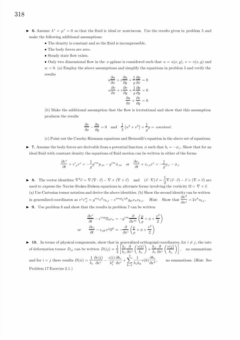
8/6/2019 Introduction to Tensor Calculus Continuum Mechanics - J. Heinbockel
http://slidepdf.com/reader/full/introduction-to-tensor-calculus-continuum-mechanics-j-heinbockel 324/372
318
6. Assume λ∗ = µ∗ = 0 so that the fluid is ideal or nonviscous. Use the results given in problem 5 and
make the following additional assumptions:
• The density is constant and so the fluid is incompressible.
• The body forces are zero.
•Steady state flow exists.
• Only two dimensional flow in the x-yplane is considered such that u = u(x, y), v = v(x, y) and
w = 0. (a) Employ the above assumptions and simplify the equations in problem 5 and verify the
results
u∂u
∂x+ v
∂u
∂y+
1
∂p
∂x= 0
u∂v
∂x+ v
∂v
∂y+
1
∂p
∂y= 0
∂u
∂x+
∂v
∂y= 0
(b) Make the additional assumption that the flow is irrotational and show that this assumption
produces the results
∂v
∂x− ∂u
∂y= 0 and
1
2
u2 + v2
+
1
p = constant.
(c) Point out the Cauchy-Riemann equations and Bernoulli’s equation in the above set of equations.
7. Assume the body forces are derivable from a potential function φ such that bi = −φ,i. Show that for an
ideal fluid with constant density the equations of fluid motion can be written in either of the forms
∂vr
∂t+ vr,svs = − 1
grm p,m − grmφ,m or
∂vr∂t
+ vr,svs = −1
p,r − φ,r
8. The vector identities ∇2v = ∇ (∇ · v) − ∇ × (∇ × v) and (v · ∇) v = 12∇ (v · v) − v × (∇ × v) are
used to express the Navier-Stokes-Duhem equations in alternate forms involving the vorticity Ω = ∇ × v.
(a) Use Cartesian tensor notation and derive the above identities. (b) Show the second identity can be written
in generalized coordinates as vjvm,j = gmjvkvk,j − mnpijkg pivnvk,j. Hint: Show that∂v2
∂xj= 2vkvk,j .
9. Use problem 8 and show that the results in problem 7 can be written
∂vr
∂t− rnpΩ pvn = −grm
∂
∂xm
p
+ φ +
v2
2
or
∂vi∂t
− ijkvjΩk = − ∂
∂xi
p
+ φ +
v2
2
10. In terms of physical components, show that in generalized orthogonal coordinates, for i = j, the rate
of deformation tensor Dij can be written D(ij) =1
2
hihj
∂
∂xj
v(i)
hi
+
hjhi
∂
∂xi
v( j)
hj
, no summations
and for i = j there results D(ii) =1
hi
∂v(i)
∂xi− v(i)
h2i
∂hi∂xi
+3
k=1
1
hihkv(k)
∂hi∂xk
, no summations. (Hint: See
Problem 17 Exercise 2.1.)

8/6/2019 Introduction to Tensor Calculus Continuum Mechanics - J. Heinbockel
http://slidepdf.com/reader/full/introduction-to-tensor-calculus-continuum-mechanics-j-heinbockel 325/372
31
Figure 2.5-6. Plane Couette flow
11. Find the physical components of the rate of deformation tensor Dij in Cartesian coordinates. (Hint:
See problem 10.)
12. Find the physical components of the rate of deformation tensor in cylindrical coordinates. (Hint: See
problem 10.)
13. (Plane Couette flow) Assume a viscous fluid with constant density is between two plates as illustrated
in the figure 2.5-6.
(a) Define ν = µ∗
as the kinematic viscosity and show the equations of fluid motion can be written
∂vi
∂t+ vi,svs = −1
gim p,m + νgjmvi,mj + gijbj , i = 1, 2, 3
(b) Let v = (u, v, w) denote the physical components of the fluid flow and make the following assumptions
• u = u(y), v = w = 0
• Steady state flow exists
• The top plate, with area A, is a distance above the bottom plate. The bottom plate is fixed and
a constant force F is applied to the top plate to keep it moving with a velocity u0 = u().• p and are constants
• The body force components are zero.
Find the velocity u = u(y)
(c) Show the tangential stress exerted by the moving fluid isF
A= σ21 = σxy = σyx = µ∗
u0
. This
example illustrates that the stress is proportional to u0 and inversely proportional to .
14. In the continuity equation make the change of variables
t =t
τ , =
0, v =
v
v0, x =
x
L, y =
y
L, z =
z
L
and write the continuity equation in terms of the barred variables and the Strouhal parameter.
15. (Plane Poiseuille flow) Consider two flat plates parallel to one another as illustrated in the figure
2.5-7. One plate is at y = 0 and the other plate is at y = 2. Let v = (u, v, w) denote the physical components
of the fluid velocity and make the following assumptions concerning the flow The body forces are zero. The
derivative∂p
∂x= − p0 is a constant and
∂p
∂y=
∂p
∂z= 0. The velocity in the x-direction is a function of y only

8/6/2019 Introduction to Tensor Calculus Continuum Mechanics - J. Heinbockel
http://slidepdf.com/reader/full/introduction-to-tensor-calculus-continuum-mechanics-j-heinbockel 326/372
320
Figure 2.5-7. Plane Poiseuille flow
with u = u(y) and v = w = 0 with boundary values u(0) = u(2) = 0. The density is constant and ν = µ∗/
is the kinematic viscosity.
(a) Show the equation of fluid motion is ν d2u
dy2+
p0
= 0, u(0) = u(2) = 0
(b) Find the velocity u = u(y) and find the maximum velocity in the x-direction. (c) Let M denote the
mass flow rate across the plane x = x0 = constant, , where 0 ≤ y ≤ 2, and 0 ≤ z ≤ 1.
Show that M =2
3µ∗p03. Note that as µ∗ increases, M decreases.
16. The heat equation (or diffusion equation) can be expressed div ( k grad u)+ H =∂ (δcu)
∂t, where c is the
specific heat [cal/gmC], δ is the volume density [gm/cm3], H is the rate of heat generation [cal/seccm3], u
is the temperature [C], k is the thermal conductivity [cal/seccmC]. Assume constant thermal conductivity,
volume density and specific heat and express the boundary value problem
k∂ 2u
∂x2= δc
∂u
∂t, 0 < x < L
u(0, t) = 0, u(L, t) = u1, u(x, 0) = f (x)
in a form where all the variables are dimensionless. Assume u1 is constant.
17. Simplify the Navier-Stokes-Duhem equations using the assumption that there is incompressible flow.
18. (Rayleigh impulsive flow) The figure 2.5-8 illustrates fluid motion in the plane where y > 0 above a
plate located along the axis where y = 0. The plate along y = 0 has zero velocity for all negative time and
at time t = 0 the plate is given an instantaneous velocity u0 in the positive x-direction. Assume the physical
components of the velocity are v = (u, v, w) which satisfy u = u(y, t), v = w = 0. Assume that the density
of the fluid is constant, the gradient of the pressure is zero, and the body forces are zero. (a) Show that the
velocity in the x-direction is governed by the differential equation
∂u∂t
= ν ∂ 2u∂y2
, with ν = µ∗
.
Assume u satisfies the initial condition u(0, t) = u0H (t) where H is the Heaviside step function. Also assume
there exist a condition at infinity limy→∞ u(y, t). This latter condition requires a bounded velocity at infinity.
(b) Use any method to show the velocity is
u(y, t) = u0 − u0 erf
y
2√
νt
= u0 erfc
y
2√
νt
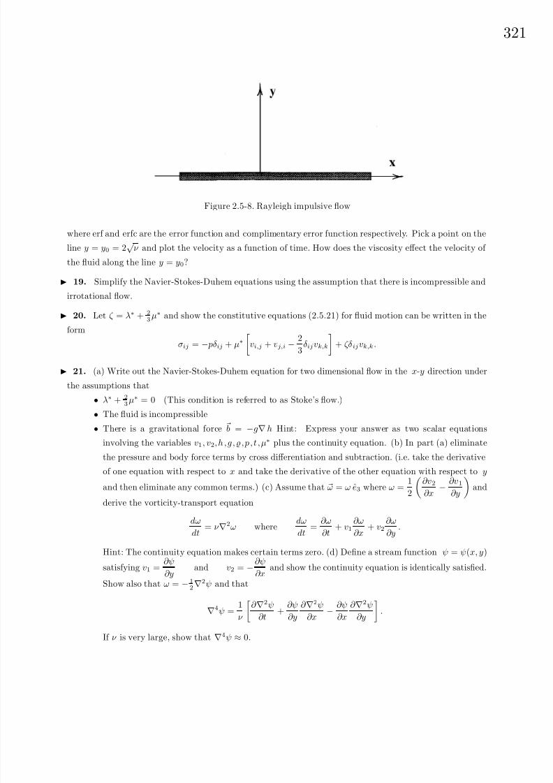
8/6/2019 Introduction to Tensor Calculus Continuum Mechanics - J. Heinbockel
http://slidepdf.com/reader/full/introduction-to-tensor-calculus-continuum-mechanics-j-heinbockel 327/372
32
Figure 2.5-8. Rayleigh impulsive flow
where erf and erfc are the error function and complimentary error function respectively. Pick a point on the
line y = y0 = 2√
ν and plot the velocity as a function of time. How does the viscosity effect the velocity of
the fluid along the line y = y0?
19. Simplify the Navier-Stokes-Duhem equations using the assumption that there is incompressible and
irrotational flow.
20. Let ζ = λ∗ + 23
µ∗ and show the constitutive equations (2.5.21) for fluid motion can be written in the
form
σij = − pδij + µ∗
vi,j + vj,i − 2
3δijvk,k
+ ζδijvk,k.
21. (a) Write out the Navier-Stokes-Duhem equation for two dimensional flow in the x-y direction under
the assumptions that
• λ∗ + 23
µ∗ = 0 (This condition is referred to as Stoke’s flow.)
• The fluid is incompressible
• There is a gravitational force b = −g∇ h Hint: Express your answer as two scalar equations
involving the variables v1, v2, h, g, , p, t , µ∗ plus the continuity equation. (b) In part (a) eliminate
the pressure and body force terms by cross differentiation and subtraction. (i.e. take the derivative
of one equation with respect to x and take the derivative of the other equation with respect to y
and then eliminate any common terms.) (c) Assume that ω = ω e3 where ω =1
2
∂v2∂x
− ∂v1∂y
and
derive the vorticity-transport equation
dω
dt= ν ∇2ω where
dω
dt=
∂ω
∂t+ v1
∂ω
∂x+ v2
∂ω
∂y.
Hint: The continuity equation makes certain terms zero. (d) Define a stream function ψ = ψ(x, y)
satisfying v1 =∂ψ
∂yand v2 = −∂ψ
∂xand show the continuity equation is identically satisfied.
Show also that ω = −12∇2ψ and that
∇4ψ =1
ν
∂ ∇2ψ
∂t+
∂ψ
∂y
∂ ∇2ψ
∂x− ∂ψ
∂x
∂ ∇2ψ
∂y
.
If ν is very large, show that ∇4ψ ≈ 0.

8/6/2019 Introduction to Tensor Calculus Continuum Mechanics - J. Heinbockel
http://slidepdf.com/reader/full/introduction-to-tensor-calculus-continuum-mechanics-j-heinbockel 328/372
322
22. In generalized orthogonal coordinates, show that the physical components of the rate of deformation
stress can be written, for i = j
σ(ij) = µ∗
hihj
∂
∂xj
v(i)
hi
+
hjhi
∂
∂xi
v( j)
hj
, no summation,
and for i = j = k
σ(ii) = − p + 2µ∗
1
hi
∂v(i)
∂xi+
1
hihjv( j)
∂hi∂xj
+1
hihkv(k)
∂hi∂xk
+
λ∗
h1h2h3
∂
∂x1h2h3v(1) +
∂
∂x2h1h3v(2) +
∂
∂x3h1h2v(3)
, no summation
23. Find the physical components for the rate of deformation stress in Cartesian coordinates. Hint: See
problem 22.
24. Find the physical components for the rate of deformations stress in cylindrical coordinates. Hint: See
problem 22. 25. Verify the Navier-Stokes equations for an incompressible fluid can be written vi = −1
p,i+ νvi,mm + bi
where ν = µ∗
is called the kinematic viscosity.
26. Verify the Navier-Stokes equations for a compressible fluid with zero bulk viscosity can be written
vi = − 1
p,i +
ν
3vm,mi + νvi,mm + bi with ν = µ∗
the kinematic viscosity.
27. The constitutive equation for a certain non-Newtonian Stokesian fluid is σij = − pδij+βDij+γDikDkj .
Assume that β and γ are constants (a) Verify that σij,j = − p,i + βDij,j + γ (DikDkj,j + Dik,jDkj)
(b) Write out the Cauchy equations of motion in Cartesian coordinates. (See page 236).
28. Let the constitutive equations relating stress and strain for a solid material take into account thermalstresses due to a temperature T . The constitutive equations have the form eij =
1 + ν
E σij− ν
E σkk δij+α T δij
where α is a coefficient of linear expansion for the material and T is the absolute temperature. Solve for the
stress in terms of strains.
29. Derive equation (2.5.53) and then show that when the bulk coefficient of viscosity is zero, the Navier-
Stokes equations, in Cartesian coordinates, can be written in the conservation form
∂ (u)
∂t+
∂ (u2 + p − τ xx)
∂x+
∂ (uv − τ xy)
∂y+
∂ (uw − τ xz)
∂z= bx
∂ (v)
∂t+
∂ (uv − τ xy)
∂x+
∂ (v2 + p − τ yy)
∂y+
∂ (vw − τ yz)
∂z= by
∂ (w)
∂t+
∂ (uw − τ xz)
∂x+
∂ (vw − τ yz)
∂y+
∂ (w2 + p − τ zz)
∂z= bz
where v1 = u,v2 = v,v3 = w and τ ij = µ∗(vi,j + vj,i − 2
3δijvk,k). Hint: Alternatively, consider 2.5.29 and use
the continuity equation.
8/6/2019 Introduction to Tensor Calculus Continuum Mechanics - J. Heinbockel
http://slidepdf.com/reader/full/introduction-to-tensor-calculus-continuum-mechanics-j-heinbockel 329/372
32
30. Show that for a perfect gas, where λ∗ = −23µ∗ and η = µ∗ is a function of position, the vector form
of equation (2.5.25) is
Dv
Dt= b − ∇ p +
4
3∇(η∇ · v) + ∇(v · ∇η) − v ∇2η + (∇η) × (∇ × v) − (∇ · v)∇η − ∇ × (∇ × (ηv))
31. Derive the energy equation D hDt
= D pDt
+ ∂Q∂t
− ∇ · q + Φ. Hint: Use the continuity equation.
32. Show that in Cartesian coordinates the Navier-Stokes equations of motion for a compressible fluid
can be written
ρDu
Dt=ρbx − ∂p
∂x+
∂
∂x
2µ∗
∂u
∂x+ λ∗∇ · V
+
∂
∂y
µ∗(
∂u
∂y+
∂v
∂x)
+
∂
∂z
µ∗(
∂w
∂x+
∂u
∂z)
ρ
Dv
Dt=ρby − ∂p
∂y+
∂
∂y
2µ∗
∂v
∂y+ λ∗∇ · V
+
∂
∂z
µ∗(
∂v
∂z+
∂w
∂y)
+
∂
∂x
µ∗(
∂w
∂y+
∂w
∂x)
ρ
Dv
Dt=ρbz − ∂p
∂z+
∂
∂z
2µ∗
∂w
∂z+ λ∗∇ · V
+
∂
∂x
µ∗(
∂w
∂x+
∂u
∂z)
+
∂
∂y
µ∗(
∂v
∂z+
∂w
∂y)
where (V x, V y, V z) = (u, v, w).
33. Show that in cylindrical coordinates the Navier-Stokes equations of motion for a compressible fluid
can be written
DV rDt
− V 2θr
=br − ∂p
∂r+
∂
∂r
2µ∗
∂V r∂r
+ λ∗∇ · V
+
1
r
∂
∂θ
µ∗(
1
r
∂V r∂θ
+∂V θ∂r
− V θr
)
+
∂
∂z
µ∗(
∂V r∂z
+∂V z∂r
)
+
2µ∗
r(
∂V r∂r
− 1
r
∂V θ∂θ
− V rr
)
DV θDt
+V rV θ
r
=bθ − 1
r
∂p
∂θ+
1
r
∂
∂θ
2µ∗(
1
r
∂V θ∂θ
+V rr
) + λ∗∇ · V
+
∂
∂z
µ∗(
1
r
∂V z∂θ
+∂V θ∂z
)
+
∂
∂r µ∗
(
1
r
∂V r
∂θ +
∂V θ
∂r −V θ
r )+
2µ∗
r (
1
r
∂V r
∂θ +
∂V θ
∂r −V θ
r )
DV zDt
=bz − ∂p
∂z+
∂
∂z
2µ∗
∂V z∂z
+ λ∗∇ · V
+
1
r
∂
∂r
µ∗r(
∂V r∂z
+∂V z∂r
)
+
1
r
∂
∂θ
µ∗(
1
r
∂V z∂θ
+∂V θ∂z
)
34. Show that the dissipation function Φ can be written as Φ = 2µ∗DijDij + λ∗Θ2.
35. Verify the identities:
(a) D
Dt(et/) =
∂et∂t
+ ∇ · (et V ) (b) D
Dt(et/) =
De
Dt+
D
Dt V 2/2
.
36. Show that the conservation law for heat flow is given by
∂T
∂t+ ∇ · (T v − κ∇T ) = S Q
where κ is the thermal conductivity of the material, T is the temperature, J advection = T v,
J conduction = −κ∇T and S Q is a source term. Note that in a solid material there is no flow and so v = 0 and

8/6/2019 Introduction to Tensor Calculus Continuum Mechanics - J. Heinbockel
http://slidepdf.com/reader/full/introduction-to-tensor-calculus-continuum-mechanics-j-heinbockel 330/372
324
the above equation reduces to the heat equation. Assign units of measurements to each term in the above
equation and make sure the equation is dimensionally homogeneous.
37. Show that in spherical coordinates the Navier-Stokes equations of motion for a compressible fluid can
be written
(DV ρDt −
V 2θ + V 2φρ ) = bρ −
∂p
∂ρ +∂
∂ρ 2µ∗∂V ρ
∂ρ + λ∗
∇ · V +1
ρ
∂
∂θ µ∗
(ρ∂
∂ρ (V θ/ρ) +1
ρ
∂V ρ∂θ )
+1
ρ sin θ
∂
∂φ
µ∗(
1
ρ sin θ
∂V ρ∂φ
+ ρ∂
∂ρ(V φ/ρ))
+
µ∗
ρ(4
∂V ρ∂ρ
− 2
ρ
∂V θ∂θ
− 4V ρρ
− 2
ρ sin θ
∂V φ∂φ
− 2V θ cot θ
ρ+ ρ cot θ
∂
∂ρ(V θ/ρ) +
cot θ
ρ
∂V ρ∂θ
)
(DV θDt
+V ρV θ
ρ−V 2φ cot θ
ρ) = bθ − 1
ρ
∂p
∂θ+
1
ρ
∂
∂θ
2µ∗
ρ(
∂V θ∂θ
+ V ρ) + λ∗∇ · V
+
1
ρ sin θ
∂
∂φ
µ∗(
sin θ
ρ
∂
∂θ(V φ/ sin θ) +
1
ρ sin θ
∂V θ∂φ
)
+
∂
∂ρ
µ∗(ρ
∂
∂ρ(V θ/ρ) +
1
ρ
∂V ρ∂θ
)
+
µ∗
ρ 21
ρ
∂V θ∂θ
− 1
ρ sin θ
∂V φ∂φ
− V θ cot θ
ρ cot θ + 3ρ∂
∂ρ(V θ/ρ) +
1
ρ
∂V ρ∂θ
DV φ
Dt+
V φV ρρ
+V θV φ cot θ
ρ
= bφ − 1
ρ sin θ
∂p
∂φ+
∂
∂ρ
µ∗ 1
ρ sin θ
∂V ρ∂φ
+ ρ∂
∂ρ(V φ/ρ)
+
1
ρ sin θ
∂
∂φ
2µ∗
ρ
1
sin θ
∂V φ∂φ
+ V ρ + V θ cot θ
+ λ∗∇ · V
+
1
ρ
∂
∂θ
µ∗
sin θ
ρ
∂
∂θ(V φ/ sin θ) +
1
ρ sin θ
∂V θ∂φ
+
µ∗
ρ
3
1
ρ sin θ
∂V ρ∂φ
+ ρ∂
∂ρ(V φ/ρ)
+ 2 cot θ
sin θ
ρ
∂
∂θ(V φ/ sin θ) +
1
ρ sin θ
∂V θ∂φ
38. Verify all the equations (2.5.28).
39. Use the conservation of energy equation (2.5.47) together with the momentum equation (2.5.25) to
derive the equation (2.5.48).
40. Verify the equation (2.5.55).
41. Consider nonviscous flow and write the 3 linear momentum equations and the continuity equation
and make the following assumptions: (i) The density is constant. (ii) Body forces are zero. (iii) Steady
state flow only. (iv) Consider only two dimensional flow with non-zero velocity components u = u(x, y) and
v = v(x, y). Show that there results the system of equations
u∂u
∂x+ v
∂u
∂y+
1
∂P
∂x= 0, u
∂v
∂x+ v
∂v
∂y+
1
∂P
∂y= 0,
∂u
∂x+
∂v
∂y= 0.
Recognize that the last equation in the above set as one of the Cauchy-Riemann equations that f (z) = u− iv
be an analytic function of a complex variable. Further assume that the fluid flow is irrotational so that∂v
∂x− ∂u
∂y= 0. Show that this implies that
1
2
u2 + v2
+
P
= Constant. If in addition u and v are derivable
from a potential function φ(x, y), such that u = ∂φ∂x and v = ∂φ
∂y , then show that φ is a harmonic function.
By constructing the conjugate harmonic function ψ(x, y) the complex potential F (z) = φ(x, y) + iψ(x, y) is
such that F (z) = u(x, y) − iv(x, y) and F (z) gives the velocity. The family of curves φ(x, y) =constant are
called equipotential curves and the family of curves ψ(x, y) = constant are called streamlines. Show that
these families are an orthogonal family of curves.
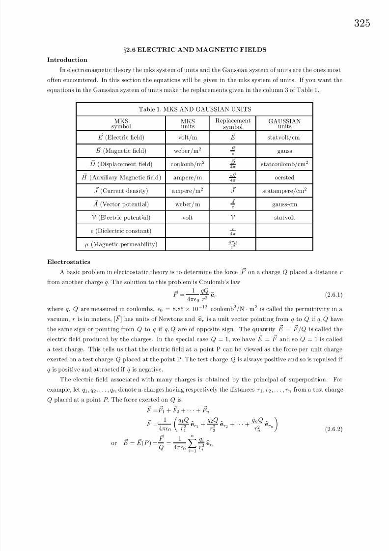
8/6/2019 Introduction to Tensor Calculus Continuum Mechanics - J. Heinbockel
http://slidepdf.com/reader/full/introduction-to-tensor-calculus-continuum-mechanics-j-heinbockel 331/372
32
§2.6 ELECTRIC AND MAGNETIC FIELDS
Introduction
In electromagnetic theory the mks system of units and the Gaussian system of units are the ones most
often encountered. In this section the equations will be given in the mks system of units. If you want the
equations in the Gaussian system of units make the replacements given in the column 3 of Table 1.
Table 1. MKS AND GAUSSIAN UNITS
MKSsymbol
MKSunits
Replacementsymbol
GAUSSIANunits
E (Electric field) volt/m E statvolt/cm
B (Magnetic field) weber/m2 Bc gauss
D (Displacement field) coulomb/m2 D4π statcoulomb/cm2
H (Auxiliary Magnetic field) ampere/m c H 4π oersted
J (Current density) ampere/m
2 J statampere/cm
2
A (Vector potential) weber/m Ac gauss-cm
V (Electric potential) volt V statvolt
(Dielectric constant) 4π
µ (Magnetic permeability) 4πµc2
Electrostatics
A basic problem in electrostatic theory is to determine the force F on a charge Q placed a distance r
from another charge q. The solution to this problem is Coulomb’s law
F = 14π0
qQr2er (2.6.1)
where q, Q are measured in coulombs, 0 = 8.85 × 10⁻¹² coulomb2/N · m2 is called the permittivity in a
vacuum, r is in meters, [ F ] has units of Newtons and er is a unit vector pointing from q to Q if q, Q have
the same sign or pointing from Q to q if q, Q are of opposite sign. The quantity E = F /Q is called the
electric field produced by the charges. In the special case Q = 1, we have E = F and so Q = 1 is called
a test charge. This tells us that the electric field at a point P can be viewed as the force per unit charge
exerted on a test charge Q placed at the point P. The test charge Q is always positive and so is repulsed if
q is positive and attracted if q is negative.
The electric field associated with many charges is obtained by the principal of superposition. For
example, let q1, q2, . . . , qn denote n-charges having respectively the distances r1, r2, . . . , rn from a test charge
Q placed at a point P. The force exerted on Q is
F = F 1 + F 2 + · · · + F n
F =1
4π0
q1Q
r21 er1 +
q2Q
r22 er2 + · · · +
qnQ
r2n ern
or E = E (P ) =
F
Q=
1
4π0
ni=1
qir2i eri
(2.6.2)

8/6/2019 Introduction to Tensor Calculus Continuum Mechanics - J. Heinbockel
http://slidepdf.com/reader/full/introduction-to-tensor-calculus-continuum-mechanics-j-heinbockel 332/372
326
where E = E (P ) is the electric field associated with the system of charges. The equation (2.6.2) can be gen-
eralized to other situations by defining other types of charge distributions. We introduce a line charge density
λ∗, (coulomb/m), a surface charge density µ∗, (coulomb/m2), a volume charge density ρ∗, (coulomb/m3),
then we can calculate the electric field associated with these other types of charge distributions. For example,
if there is a charge distribution λ∗ = λ∗(s) along a curve C , where s is an arc length parameter, then we
would have
E (P ) =1
4π0
C
er
r2λ∗ds (2.6.3)
as the electric field at a point P due to this charge distribution. The integral in equation (2.6.3) being a
line integral along the curve C and where ds is an element of arc length. Here equation (2.6.3) represents a
continuous summation of the charges along the curve C. For a continuous charge distribution over a surface
S , the electric field at a point P is
E (P ) =1
4π0
S
er
r2µ∗dσ (2.6.4)
where dσ represents an element of surface area on S . Similarly, if ρ∗ represents a continuous charge distri-
bution throughout a volume V , then the electric field is represented
E (P ) =1
4π0
V
er
r2ρ∗ dτ (2.6.5)
where dτ is an element of volume. In the equations (2.6.3), (2.6.4), (2.6.5) we let (x, y, z) denote the position
of the test charge and let (x, y, z) denote a point on the line, on the surface or within the volume, then
r = (x − x) e1 + (y − y) e2 + (z − z) e3 (2.6.6)
represents the distance from the point P to an element of charge λ∗ds, µ∗dσ or ρ∗dτ with r = |r| and
er =
r
r.
If the electric field is conservative, then∇ ×
E = 0, and so it is derivable from a potential functionV
by taking the negative of the gradient of V and
E = −∇V . (2.6.7)
For these conditions note that ∇V · dr = − E · dr is an exact differential so that the potential function can
be represented by the line integral
V = V (P ) = − P
α
E · dr (2.6.8)
where α is some reference point (usually infinity, where V (∞) = 0). For a conservative electric field the line
integral will be independent of the path connecting any two points a and b so that
V (b) − V (a) = − bα
E · dr −
− aα
E · dr
= −
ba
E · dr =
ba
∇V · dr. (2.6.9)
Let α = ∞ in equation (2.6.8), then the potential function associated with a point charge moving in
the radial direction er is
V (r) = − r∞
E · dr =−q
4π0
r∞
1
r2dr =
q
4π0
1
r|r∞=
q
4π0r.
8/6/2019 Introduction to Tensor Calculus Continuum Mechanics - J. Heinbockel
http://slidepdf.com/reader/full/introduction-to-tensor-calculus-continuum-mechanics-j-heinbockel 333/372
32
By superposition, the potential at a point P for a continuous volume distribution of charges is given by
V (P ) =1
4π0
V
ρ∗
rdτ and for a surface distribution of charges V (P ) =
1
4π0
S
µ∗
rdσ and for a line
distribution of charges V (P ) =1
4π0
C
λ∗
rds; and for a discrete distribution of point charges
V (P ) =
1
4π0
N
i=1 qi
ri. When the potential functions are defined from a common reference point, then the
principal of superposition applies.
The potential function V is related to the work done W in moving a charge within the electric field.
The work done in moving a test charge Q from point a to point b is an integral of the force times distance
moved. The electric force on a test charge Q is F = Q E and so the force F = −Q E is in opposition to this
force as you move the test charge. The work done is
W =
ba
F · dr =
ba
−Q E · dr = Q
ba
∇V · dr = Q[V (b) − V (a)]. (2.6.10)
The work done is independent of the path joining the two points and depends only on the end points and
the change in the potential. If one moves Q from infinity to point b, then the above becomes W = QV (b).
An electric field E = E (P ) is a vector field which can be represented graphically by constructing vectors
at various selected points in the space. Such a plot is called a vector field plot. A field line associated with
a vector field is a curve such that the tangent vector to a point on the curve has the same direction as the
vector field at that point. Field lines are used as an aid for visualization of an electric field and vector fields
in general. The tangent to a field line at a point has the same direction as the vector field E at that point.
For example, in two dimensions let r = x e1 + y e2 denote the position vector to a point on a field line. The
tangent vector to this point has the direction dr = dx e1 + dy e2. If E = E (x, y) = −N (x, y) e1 + M (x, y) e2is the vector field constructed at the same point, then E and dr must be colinear. Thus, for each point (x, y)
on a field line we require that dr = K E for some constant K . Equating like components we find that the
field lines must satisfy the differential relation.
dx
−N (x, y)=
dy
M (x, y)=K
or M (x, y) dx + N (x, y) dy =0.
(2.6.11)
In two dimensions, the family of equipotential curves V (x, y) = C 1 =constant, are orthogonal to the family
of field lines and are described by solutions of the differential equation
N (x, y) dx − M (x, y) dy = 0
obtained from equation (2.6.11) by taking the negative reciprocal of the slope. The field lines are perpendic-
ular to the equipotential curves because at each point on the curve V = C 1 we have ∇V being perpendicular
to the curve V = C 1 and so it is colinear with E at this same point. Field lines associated with electric
fields are called electric lines of force. The density of the field lines drawn per unit cross sectional area are
proportional to the magnitude of the vector field through that area.

8/6/2019 Introduction to Tensor Calculus Continuum Mechanics - J. Heinbockel
http://slidepdf.com/reader/full/introduction-to-tensor-calculus-continuum-mechanics-j-heinbockel 334/372
328
Figure 2.6-1. Electric forces due to a positive charge at (−a, 0) and negative charge at (a, 0).
EXAMPLE 2.6-1.
Find the field lines and equipotential curves associated with a positive charge q located at the point
(−a, 0) and a negative charge −q located at the point (a, 0).
Solution: With reference to the figure 2.6-1, the total electric force E on a test charge Q = 1 place
at a general point (x, y) is, by superposition, the sum of the forces from each of the isolated charges and is
E = E 1 + E 2. The electric force vectors due to each individual charge are
E 1 =kq(x + a)
e1 + kqy
e2
r31
with r21 = (x + a)2 + y2
E 2 =−kq(x − a) e1 − kqy e2
r32with r22 = (x − a)2 + y2
(2.6.12)
where k =1
4π0is a constant. This gives
E = E 1 + E 2 =
kq(x + a)
r31− kq(x − a)
r32
e1 +
kqy
r31− kqy
r32
e2.
This determines the differential equation of the field lines
dx
kq(x+a)r31
− kq(x−a)r32
=
dy
kqyr31
− kqyr32
. (2.6.13)
To solve this differential equation we make the substitutions
cos θ1 =x + a
r1and cos θ2 =
x − a
r2(2.6.14)

8/6/2019 Introduction to Tensor Calculus Continuum Mechanics - J. Heinbockel
http://slidepdf.com/reader/full/introduction-to-tensor-calculus-continuum-mechanics-j-heinbockel 335/372
32
Figure 2.6-2. Lines of electric force between two opposite sign charges.
as suggested by the geometry from figure 2.6-1. From the equations (2.6.12) and (2.6.14) we obtain the
relations
− sin θ1 dθ1 =r1dx − (x + a) dr1
r21
2r1dr1 =2(x + a) dx + 2ydy
− sin θ2 dθ2 =r2 dx − (x − a)dr2
r22
2r2 dr2 =2(x − a) dx + 2y dy
which implies that
− sin θ1 dθ1 = −(x + a)y dy
r31 +
y2 dx
r31
− sin θ2 dθ2 = − (x − a)y dy
r32+
y2 dx
r32
(2.6.15)
Now compare the results from equation (2.6.15) with the differential equation (2.6.13) and determine that
y is an integrating factor of equation (2.6.13) . This shows that the differential equation (2.6.13) can be
written in the much simpler form of the exact differential equation
− sin θ1 dθ1 + sin θ2 dθ2 = 0 (2.6.16)
in terms of the variables θ1 and θ2. The equation (2.6.16) is easily integrated to obtain
cos θ1 − cos θ2 = C (2.6.17)
where C is a constant of integration. In terms of x, y the solution can be written
x + a (x + a)2 + y2
− x − a (x − a)2 + y2
= C. (2.6.18)
These field lines are illustrated in the figure 2.6-2.

8/6/2019 Introduction to Tensor Calculus Continuum Mechanics - J. Heinbockel
http://slidepdf.com/reader/full/introduction-to-tensor-calculus-continuum-mechanics-j-heinbockel 336/372
330
The differential equation for the equipotential curves is obtained by taking the negative reciprocal of
the slope of the field lines. This gives
dy
dx=
kq(x−a)r32
− kq(x+a)r31
kqyr31
− kqyr32
.
This result can be written in the form
−
(x + a)dx + ydy
r31
+
(x − a)dx + ydy
r32
= 0
which simplifies to the easily integrable form
−dr1r21
+dr2r22
= 0
in terms of the new variables r1 and r2. An integration produces the equipotential curves
1
r1 −1
r2=C 2
or1
(x + a)2 + y2− 1
(x − a)2 + y2=C 2.
The potential function for this problem can be interpreted as a superposition of the potential functions
V 1 = −kq
r1and V 2 =
kq
r2associated with the isolated point charges at the points (−a, 0) and (a, 0).
Observe that the electric lines of force move from positive charges to negative charges and they do not
cross one another. Where field lines are close together the field is strong and where the lines are far apart
the field is weak. If the field lines are almost parallel and equidistant from one another the field is said to be
uniform. The arrows on the field lines show the direction of the electric field E . If one moves along a field
line in the direction of the arrows the electric potential is decreasing and they cross the equipotential curves
at right angles. Also, when the electric field is conservative we will have ∇ × E = 0.
In three dimensions the situation is analogous to what has been done in two dimensions. If the electric
field is E = E (x, y, z) = P (x, y, z) e1 + Q(x, y, z) e2 + R(x, y, z) e3 and r = x e1 + y e2 + z e3 is the position
vector to a variable point (x, y, z) on a field line, then at this point dr and E must be colinear so that
dr = K E for some constant K . Equating like coefficients gives the system of equations
dx
P (x, y, z)=
dy
Q(x, y, z)=
dz
R(x, y, z)= K. (2.6.19)
From this system of equations one must try to obtain two independent integrals, call them u1(x, y, z) = c1
and u2(x, y, z) = c2. These integrals represent one-parameter families of surfaces. When any two of these
surfaces intersect, the result is a curve which represents a field line associated with the vector field E. These
type of field lines in three dimensions are more difficult to illustrate.
The electric flux φE of an electric field E over a surface S is defined as the summation of the normal
component of E over the surface and is represented
φE =
S
E · n dσ with units of N m2
C (2.6.20)
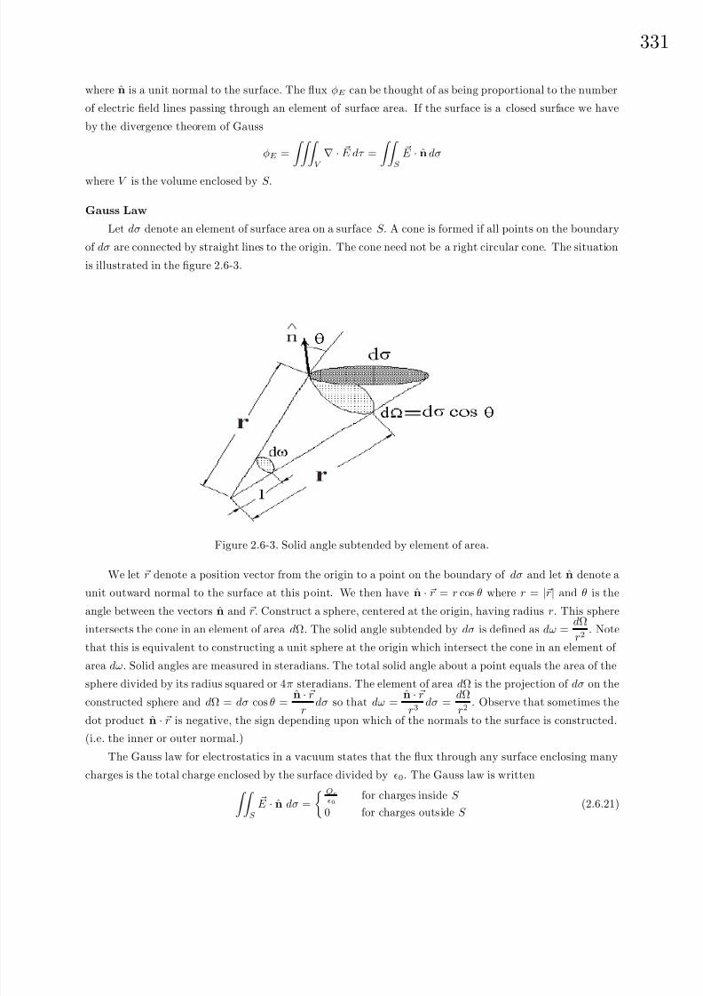
8/6/2019 Introduction to Tensor Calculus Continuum Mechanics - J. Heinbockel
http://slidepdf.com/reader/full/introduction-to-tensor-calculus-continuum-mechanics-j-heinbockel 337/372
33
where n is a unit normal to the surface. The flux φE can be thought of as being proportional to the number
of electric field lines passing through an element of surface area. If the surface is a closed surface we have
by the divergence theorem of Gauss
φE =
V ∇ · E dτ =
S E · n dσ
where V is the volume enclosed by S.
Gauss Law
Let dσ denote an element of surface area on a surface S. A cone is formed if all points on the boundary
of dσ are connected by straight lines to the origin. The cone need not be a right circular cone. The situation
is illustrated in the figure 2.6-3.
Figure 2.6-3. Solid angle subtended by element of area.
We let r denote a position vector from the origin to a point on the boundary of dσ and let n denote a
unit outward normal to the surface at this point. We then have n · r = r cos θ where r = |r| and θ is the
angle between the vectors n and r. Construct a sphere, centered at the origin, having radius r. This sphere
intersects the cone in an element of area dΩ. The solid angle subtended by dσ is defined as dω =dΩ
r2. Note
that this is equivalent to constructing a unit sphere at the origin which intersect the cone in an element of
area dω. Solid angles are measured in steradians. The total solid angle about a point equals the area of the
sphere divided by its radius squared or 4π steradians. The element of area dΩ is the projection of dσ on the
constructed sphere and dΩ = dσ cos θ = n · rr
dσ so that dω = n · rr3
dσ = dΩr2
. Observe that sometimes the
dot product n · r is negative, the sign depending upon which of the normals to the surface is constructed.
(i.e. the inner or outer normal.)
The Gauss law for electrostatics in a vacuum states that the flux through any surface enclosing many
charges is the total charge enclosed by the surface divided by 0. The Gauss law is written S
E · n dσ =
Qe
0for charges inside S
0 for charges outside S (2.6.21)

8/6/2019 Introduction to Tensor Calculus Continuum Mechanics - J. Heinbockel
http://slidepdf.com/reader/full/introduction-to-tensor-calculus-continuum-mechanics-j-heinbockel 338/372
332
where Qe represents the total charge enclosed by the surface S with n the unit outward normal to the surface.
The proof of Gauss’s theorem follows. Consider a single charge q within the closed surface S. The electric
field at a point on the surface S due to the charge q within S is represented E =1
4π0
q
r2er and so the flux
integral is
φE = S E
·n dσ = S
q
4π0 er · n
r2
dσ =q
4π0 SdΩ
r2
=q
0(2.6.22)
sinceer · n
r2=
cos θ dσ
r2=
dΩ
r2= dω and
S
dω = 4π. By superposition of the charges, we obtain a similar
result for each of the charges within the surface. Adding these results gives Qe =
ni=1
qi. For a continuous
distribution of charge inside the volume we can write Qe =
V
ρ∗ dτ , where ρ∗ is the charge distribution
per unit volume. Note that charges outside of the closed surface do not contribute to the total flux across
the surface. This is because the field lines go in one side of the surface and go out the other side. In this
case
S
E · n dσ = 0 for charges outside the surface. Also the position of the charge or charges within the
volume does not effect the Gauss law.
The equation (2.6.21) is the Gauss law in integral form. We can put this law in differential form as
follows. Using the Gauss divergence theorem we can write for an arbitrary volume that S
E · n dσ =
V
∇ · E dτ =
V
ρ∗
0dτ =
Qe
0=
1
0
V
ρ∗ dτ
which for an arbitrary volume implies
∇ · E =ρ∗
0. (2.6.23)
The equations (2.6.23) and (2.6.7) can be combined so that the Gauss law can also be written in the form
∇2V = − ρ∗
0which is called Poisson’s equation.
EXAMPLE 2.6-2
Find the electric field associated with an infinite plane sheet of positive charge.
Solution: Assume there exists a uniform surface charge µ∗ and draw a circle at some point on the plane
surface. Now move the circle perpendicular to the surface to form a small cylinder which extends equal
distances above and below the plane surface. We calculate the electric flux over this small cylinder in the
limit as the height of the cylinder goes to zero. The charge inside the cylinder is µ∗A where A is the area of
the circle. We find that the Gauss law requires that S
E · n dσ =Qe
0=
µ∗A
0(2.6.24)
where n is the outward normal to the cylinder as we move over the surface S. By the symmetry of thesituation the electric force vector is uniform and must point away from both sides to the plane surface in the
direction of the normals to both sides of the surface. Denote the plane surface normals by en and − en and
assume that E = β en on one side of the surface and E = −β en on the other side of the surface for some
constant β . Substituting this result into the equation (2.6.24) produces S
E · n dσ = 2βA (2.6.25)

8/6/2019 Introduction to Tensor Calculus Continuum Mechanics - J. Heinbockel
http://slidepdf.com/reader/full/introduction-to-tensor-calculus-continuum-mechanics-j-heinbockel 339/372
33
since only the ends of the cylinder contribute to the above surface integral. On the sides of the cylinder we
will have n · ± en = 0 and so the surface integral over the sides of the cylinder is zero. By equating the
results from equations (2.6.24) and (2.6.25) we obtain the result that β =µ∗
20and consequently we can write
E =µ∗
20 en where
en represents one of the normals to the surface.
Note an electric field will always undergo a jump discontinuity when crossing a surface charge µ∗. As in
the above example we have E up =µ∗
20 en and E down = −µ∗
2en so that the difference is
E up − E down =µ∗
0 en or E in
(1)i + E in
(2)i +
µ∗
0= 0. (2.6.26)
It is this difference which causes the jump discontinuity.
EXAMPLE 2.6-3.
Calculate the electric field associated with a uniformly charged sphere of radius a.
Solution: We proceed as in the previous example. Let µ∗ denote the uniform charge distribution over the
surface of the sphere and let er denote the unit normal to the sphere. The total charge then is written asq =
Sa
µ∗dσ = 4πa2µ∗. If we construct a sphere of radius r > a around the charged sphere, then we have
by the Gauss theorem Sr
E · er dσ =Qe
0=
q
0. (2.6.27)
Again, we can assume symmetry for E and assume that it points radially outward in the direction of the
surface normal er and has the form E = β er for some constant β. Substituting this value for E into the
equation (2.6.27) we find that
Sr E ·
er dσ = β
Srdσ = 4πβr2 =
q
0. (2.6.28)
This gives E =1
4π0
q
r2er where er is the outward normal to the sphere. This shows that the electric field
outside the sphere is the same as if all the charge were situated at the origin.
For S a piecewise closed surface enclosing a volume V and F i = F i(x1, x2, x3) i = 1, 2, 3, a continuous
vector field with continuous derivatives the Gauss divergence theorem enables us to replace a flux integral
of F i over S by a volume integral of the divergence of F i over the volume V such that S
F ini dσ =
V
F i,i dτ or
S
F · n dσ =
V
div F dτ. (2.6.29)
If V contains a simple closed surface Σ where F i is discontinuous we must modify the above Gauss divergence
theorem.
EXAMPLE 2.6-4.
We examine the modification of the Gauss divergence theorem for spheres in order to illustrate the
concepts. Let V have surface area S which encloses a surface Σ. Consider the figure 2.6-4 where the volume
V enclosed by S and containing Σ has been cut in half.
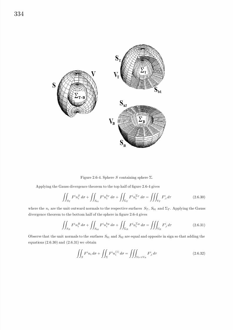
8/6/2019 Introduction to Tensor Calculus Continuum Mechanics - J. Heinbockel
http://slidepdf.com/reader/full/introduction-to-tensor-calculus-continuum-mechanics-j-heinbockel 340/372
334
Figure 2.6-4. Sphere S containing sphere Σ.
Applying the Gauss divergence theorem to the top half of figure 2.6-4 gives ST
F inT i dσ +
Sb1
F inbT i dσ +
ΣT
F inΣT
i dσ =
V T
F i,i dτ (2.6.30)
where the ni are the unit outward normals to the respective surfaces S T , S b1 and ΣT . Applying the Gauss
divergence theorem to the bottom half of the sphere in figure 2.6-4 gives
SBF inB
i dσ +
Sb2F inbB
i dσ +
ΣB
F inΣB
i dσ =
V BF i,i dτ (2.6.31)
Observe that the unit normals to the surfaces S b1 and S b2 are equal and opposite in sign so that adding the
equations (2.6.30) and (2.6.31) we obtain S
F ini dσ +
Σ
F in(1)i dσ =
V T +V B
F i,i dτ (2.6.32)
8/6/2019 Introduction to Tensor Calculus Continuum Mechanics - J. Heinbockel
http://slidepdf.com/reader/full/introduction-to-tensor-calculus-continuum-mechanics-j-heinbockel 341/372
33
where S = S T + S B is the total surface area of the outside sphere and Σ = ΣT + ΣB is the total surface area
of the inside sphere, and n(1)i is the inward normal to the sphere Σ when the top and bottom volumes are
combined. Applying the Gauss divergence theorem to just the isolated small sphere Σ we find
ΣF in
(2)i dσ = V Σ
F i,i dτ (2.6.33)
where n(2)i is the outward normal to Σ. By adding the equations (2.6.33) and (2.6.32) we find that
S
F ini dσ +
Σ
F in
(1)i + F in
(2)i
dσ =
V
F i,i dτ (2.6.34)
where V = V T + V B + V Σ. The equation (2.6.34) can also be written as S
F ini dσ =
V
F i,i dτ −
Σ
F in
(1)i + F in
(2)i
dσ. (2.6.35)
In the case that V contains a surface Σ the total electric charge inside S is
Qe =
V
ρ∗ dτ +
Σ
µ∗ dσ (2.6.36)
where µ∗ is the surface charge density on Σ and ρ∗ is the volume charge density throughout V. The Gauss
theorem requires that S
E ini dσ =Qe
0=
1
0
V
ρ∗ dτ +1
0
Σ
µ∗ dσ. (2.6.37)
In the case of a jump discontinuity across the surface Σ we use the results of equation (2.6.34) and write S
E ini dσ =
V
E i,i dτ −
Σ
E in
(1)i + E in
(2)i
dσ. (2.6.38)
Subtracting the equation (2.6.37) from the equation (2.6.38) gives V
E i,i − ρ∗
0
dτ −
Σ
E in
(1)i + E in
(2)i +
µ∗
0
dσ = 0. (2.6.39)
For arbitrary surfaces S and Σ, this equation implies the differential form of the Gauss law
E i,i =ρ∗
0. (2.6.40)
Further, on the surface Σ, where there is a surface charge distribution we have
E in(1)i + E in
(2)i +
µ∗
0= 0 (2.6.41)
which shows the electric field undergoes a discontinuity when you cross a surface charge µ∗.

8/6/2019 Introduction to Tensor Calculus Continuum Mechanics - J. Heinbockel
http://slidepdf.com/reader/full/introduction-to-tensor-calculus-continuum-mechanics-j-heinbockel 342/372
336
Electrostatic Fields in Materials
When charges are introduced into materials it spreads itself throughout the material. Materials in
which the spreading occurs quickly are called conductors, while materials in which the spreading takes a
long time are called nonconductors or dielectrics. Another electrical property of materials is the ability to
hold local charges which do not come into contact with other charges. This property is called induction.
For example, consider a single atom within the material. It has a positively charged nucleus and negatively
charged electron cloud surrounding it. When this atom experiences an electric field E the negative cloud
moves opposite to E while the positively charged nucleus moves in the direction of E . If E is large enough it
can ionize the atom by pulling the electrons away from the nucleus. For moderately sized electric fields the
atom achieves an equilibrium position where the positive and negative charges are offset. In this situation
the atom is said to be polarized and have a dipole moment p.
Definition: When a pair of charges +q and −q are separated by a distance 2 d the electric dipole
moment is defined by p = 2 dq, where p has dimensions of [C m].
In the special case where d has the same direction as E and the material is symmetric we say that p
is proportional to E and write p = α
E , where α is called the atomic polarizability. If in a material subject
to an electric field their results many such dipoles throughout the material then the dielectric is said to be
polarized. The vector quantity P is introduced to represent this effect. The vector P is called the polarization
vector having units of [C/m2], and represents an average dipole moment per unit volume of material. The
vectors P i and E i are related through the displacement vector Di such that
P i = Di − 0E i. (2.6.42)
For an anisotropic material (crystal)
Di = ji E j and P i = αji E j (2.6.43)
where ji is called the dielectric tensor and αji is called the electric susceptibility tensor. Consequently,
P i = αji E j = jiE j − 0E i = (ji − 0δj
i )E j so that αji = ji − 0δj
i . (2.6.44)
A dielectric material is called homogeneous if the electric force and displacement vector are the same for any
two points within the medium. This requires that the electric force and displacement vectors be constant
parallel vector fields. It is left as an exercise to show that the condition for homogeneity is that ji,k = 0.
A dielectric material is called isotropic if the electric force vector and displacement vector have the same
direction. This requires that ji = δij where δi
j is the Kronecker delta. The term = 0K e is called the
dielectric constant of the medium. The constant 0 = 8.85(10)−12 coul2/N · m2 is the permittivity of free
space and the quantity ke = 0
is called the relative dielectric constant (relative to 0). For free space ke = 1.
Similarly for an isotropic material we have αji = 0αeδj
i where αe is called the electric susceptibility. For a
linear medium the vectors P , D and E are related by
Di = 0E i + P i = 0E i + 0αeE i = 0(1 + αe)E i = 0K eE i = E i (2.6.45)
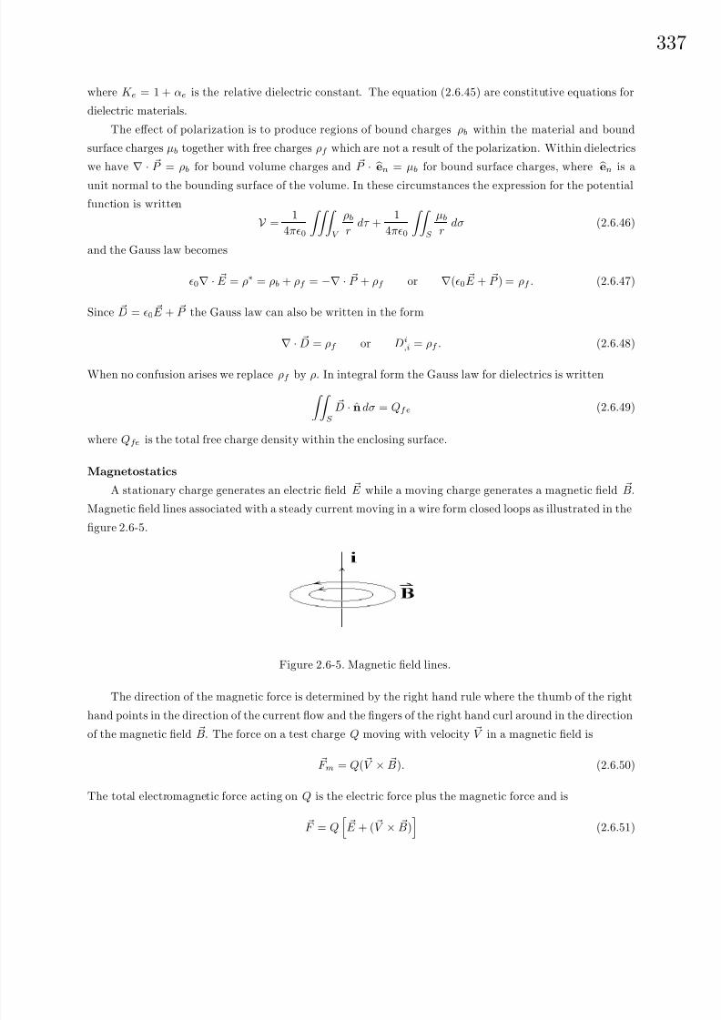
8/6/2019 Introduction to Tensor Calculus Continuum Mechanics - J. Heinbockel
http://slidepdf.com/reader/full/introduction-to-tensor-calculus-continuum-mechanics-j-heinbockel 343/372
33
where K e = 1 + αe is the relative dielectric constant. The equation (2.6.45) are constitutive equations for
dielectric materials.
The effect of polarization is to produce regions of bound charges ρb within the material and bound
surface charges µb together with free charges ρf which are not a result of the polarization. Within dielectrics
we have
∇ · P = ρb for bound volume charges and P
· en = µb for bound surface charges, where en is a
unit normal to the bounding surface of the volume. In these circumstances the expression for the potential
function is written
V =1
4π0
V
ρb
rdτ +
1
4π0
S
µb
rdσ (2.6.46)
and the Gauss law becomes
0∇ · E = ρ∗ = ρb + ρf = −∇ · P + ρf or ∇(0 E + P ) = ρf . (2.6.47)
Since D = 0 E + P the Gauss law can also be written in the form
∇ · D = ρf or Di
,i = ρf . (2.6.48)
When no confusion arises we replace ρf by ρ. In integral form the Gauss law for dielectrics is written S
D · n dσ = Qfe (2.6.49)
where Qfe is the total free charge density within the enclosing surface.
Magnetostatics
A stationary charge generates an electric field E while a moving charge generates a magnetic field B.
Magnetic field lines associated with a steady current moving in a wire form closed loops as illustrated in the
figure 2.6-5.
Figure 2.6-5. Magnetic field lines.
The direction of the magnetic force is determined by the right hand rule where the thumb of the right
hand points in the direction of the current flow and the fingers of the right hand curl around in the directionof the magnetic field B. The force on a test charge Q moving with velocity V in a magnetic field is
F m = Q( V × B). (2.6.50)
The total electromagnetic force acting on Q is the electric force plus the magnetic force and is
F = Q
E + ( V × B)
(2.6.51)

8/6/2019 Introduction to Tensor Calculus Continuum Mechanics - J. Heinbockel
http://slidepdf.com/reader/full/introduction-to-tensor-calculus-continuum-mechanics-j-heinbockel 344/372
338
which is known as the Lorentz force law. The magnetic force due to a line charge density λ∗ moving along
a curve C is the line integral
F mag =
C
λ∗ ds( V × B) =
C
I × Bds. (2.6.52)
Similarly, for a moving surface charge density moving on a surface
F mag =
S
µ∗dσ( V × B) =
S
K × B dσ (2.6.53)
and for a moving volume charge density
F mag =
V
ρ∗dτ ( V × B) =
V
J × B dτ (2.6.54)
where the quantities I = λ∗ V , K = µ∗ V and J = ρ∗ V are respectively the current, the current per unit
length, and current per unit area.
A conductor is any material where the charge is free to move. The flow of charge is governed by Ohm’s
law. Ohm’s law states that the current density vector J i is a linear function of the electric intensity or
J i = σimE m, where σim is the conductivity tensor of the material. For homogeneous, isotropic conductors
σim = σδim so that J i = σE i where σ is the conductivity and 1/σ is called the resistivity.
Surround a charge density ρ∗ with an arbitrary simple closed surface S having volume V and calculate
the flux of the current density across the surface. We find by the divergence theorem S
J · n dσ =
V
∇ · J dτ. (2.6.55)
If charge is to be conserved, the current flow out of the volume through the surface must equal the loss due
to the time rate of change of charge within the surface which implies
S
J · n dσ = V
∇ · J dτ = − ddt
V
ρ∗ dτ = − V
∂ρ∗
∂tdτ (2.6.56)
or V
∇ · J +
∂ρ∗
∂t
dτ = 0. (2.6.57)
This implies that for an arbitrary volume we must have
∇ · J = − ∂ρ∗
∂t. (2.6.58)
Note that equation (2.6.58) has the same form as the continuity equation (2.3.73) for mass conservation and
so it is also called a continuity equation for charge conservation. For magnetostatics there exists steady line
currents or stationary current so ∂ρ∗
∂t = 0. This requires that ∇ · J = 0.

8/6/2019 Introduction to Tensor Calculus Continuum Mechanics - J. Heinbockel
http://slidepdf.com/reader/full/introduction-to-tensor-calculus-continuum-mechanics-j-heinbockel 345/372
33
Figure 2.6-6. Magnetic field around wire.
Biot-Savart Law
The Biot-Savart law for magnetostatics describes the magnetic field at a point P due to a steady line
current moving along a curve C and is
B(P ) =µ0
4π
C
I × er
r2ds (2.6.59)
with units [N/amp · m] and where the integration is in the direction of the current flow. In the Biot-Savart
law we have the constant µ0 = 4π × 10−7 N/amp2 which is called the permeability of free space, I = I
et is
the current flowing in the direction of the unit tangent vector et to the curve C, er is a unit vector directed
from a point on the curve C toward the point P and r is the distance from a point on the curve to the
general point P. Note that for a steady current to exist along the curve the magnitude of I must be the
same everywhere along the curve. Hence, this term can be brought out in front of the integral. For surface
currents K and volume currents J the Biot-Savart law is written
B(P ) =µ0
4π
S
K × er
r2dσ
and B(P ) =µ0
4π
V
J × er
r2dτ.
EXAMPLE 2.6-5.
Calculate the magnetic field B a distance h perpendicular to a wire carrying a constant current I.Solution: The magnetic field circles around the wire. For the geometry of the figure 2.6-6, the magnetic
field points out of the page. We can write
I × er = I et × er = I e sin α
where e is a unit vector tangent to the circle of radius h which encircles the wire and cuts the wire perpen-
dicularly.

8/6/2019 Introduction to Tensor Calculus Continuum Mechanics - J. Heinbockel
http://slidepdf.com/reader/full/introduction-to-tensor-calculus-continuum-mechanics-j-heinbockel 346/372
340
For this problem the Biot-Savart law is
B(P ) =µ0I
4π
e
r2ds.
In terms of θ we find from the geometry of figure 2.6-6
tan θ = sh
with ds = h sec2 θ dθ and cos θ = hr
.
Therefore,
B(P ) =µ0
π
θ2θ1
I e sin α h sec2 θ
h2/ cos2 θdθ.
But, α = π/2 + θ so that sin α = cos θ and consequently
B(P ) =µ0I e
4πh
θ2θ1
cos θ dθ =µ0I e
4πh(sin θ2 − sin θ1).
For a long straight wire θ1 → −π/2 and θ2 → π/2 to give the magnetic field B(P ) =
µ0I e
2πh .
For volume currents the Biot-Savart law is
B(P ) =µ0
4π
V
J × er
r2dτ (2.6.60)
and consequently (see exercises)
∇ · B = 0. (2.6.61)
Recall the divergence of an electric field is ∇ · E = ρ∗
0is known as the Gauss’s law for electric fields and so
in analogy the divergence ∇· B = 0 is sometimes referred to as Gauss’s law for magnetic fields. If ∇· B = 0,
then there exists a vector field A such that B = ∇ × A. The vector field A is called the vector potential of B. Note that ∇ · B = ∇ · (∇ × A) = 0. Also the vector potential A is not unique since B is also derivable
from the vector potential A + ∇φ where φ is an arbitrary continuous and differentiable scalar.
Ampere’s Law
Ampere’s law is associated with the work done in moving around a simple closed path. For example,
consider the previous example 2.6-5. In this example the integral of B around a circular path of radius h
which is centered at some point on the wire can be associated with the work done in moving around this
path. The summation of force times distance is
C B · dr = C B · e ds =
µ0I
2πh C ds = µ0I (2.6.62)
where now dr = e ds is a tangent vector to the circle encircling the wire and
C
ds = 2πh is the distance
around this circle. The equation (2.6.62) holds not only for circles, but for any simple closed curve around
the wire. Using the Stoke’s theorem we have C
B · dr =
S
(∇ × B) · en dσ = µ0I =
S
µ0 J · en dσ (2.6.63)

8/6/2019 Introduction to Tensor Calculus Continuum Mechanics - J. Heinbockel
http://slidepdf.com/reader/full/introduction-to-tensor-calculus-continuum-mechanics-j-heinbockel 347/372
34
where
S
J · en dσ is the total flux (current) passing through the surface which is created by encircling
some curve about the wire. Equating like terms in equation (2.6.63) gives the differential form of Ampere’s
law
∇ × B = µ0 J. (2.6.64)
Magnetostatics in Materials
Similar to what happens when charges are introduced into materials we have magnetic fields whenever
there are moving charges within materials. For example, when electrons move around an atom tiny current
loops are formed. These current loops create what are called magnetic dipole moments m throughout the
material. When a magnetic field B is applied to a material medium there is a net alignment of the magnetic
dipoles. The quantity M , called the magnetization vector is introduced. Here M is associated with a
dielectric medium and has the units [amp/m] and represents an average magnetic dipole moment per unit
volume and is analogous to the polarization vector P used in electrostatics. The magnetization vector M
acts a lot like the previous polarization vector in that it produces bound volume currents J b and surface
currents K b where ∇ × M = J b is a volume current density throughout some volume and M × en = K b is a
surface current on the boundary of this volume.
From electrostatics note that the time derivative of 0∂ E∂t has the same units as current density. The
total current in a magnetized material is then J t = J b + J f + 0∂ E∂t where J b is the bound current, J f is the
free current and 0∂ E∂t is the induced current. Ampere’s law, equation (2.6.64), in magnetized materials then
becomes
∇ × B = µ0 J t = µ0( J b + J f + 0
∂ E
∂t) = µ0
J + µ00∂ E
∂t(2.6.65)
where J = J b + J f . The term 0∂ E∂t
is referred to as a displacement current or as a Maxwell correction to
the field equation. This term implies that a changing electric field induces a magnetic field.
An auxiliary magnet field H defined by
H i =1
µ0Bi − M i (2.6.66)
is introduced which relates the magnetic force vector B and magnetization vector M. This is another con-
stitutive equation which describes material properties. For an anisotropic material (crystal)
Bi = µji H j and M i = χj
i H j (2.6.67)
where µji is called the magnetic permeability tensor and χj
i is called the magnetic permeability tensor. Both
of these quantities are dimensionless. For an isotropic material
µji = µδji where µ = µ0km. (2.6.68)
Here µ0 = 4π × 10−7 N/amp2 is the permeability of free space and km = µµ0
is the relative permeability
coefficient. Similarly, for an isotropic material we have χji = χmδj
i where χm is called the magnetic sus-
ceptibility coefficient and is dimensionless. The magnetic susceptibility coefficient has positive values for
8/6/2019 Introduction to Tensor Calculus Continuum Mechanics - J. Heinbockel
http://slidepdf.com/reader/full/introduction-to-tensor-calculus-continuum-mechanics-j-heinbockel 348/372
342
materials called paramagnets and negative values for materials called diamagnets. For a linear medium the
quantities B, M and H are related by
Bi = µ0(H i + M i) = µ0H i + µ0χmH i = µ0(1 + χm)H i = µ0kmH i = µH i (2.6.69)
where µ = µ0km = µ0(1 + χm) is called the permeability of the material.Note: The auxiliary magnetic vector H for magnetostatics in materials plays a role similar to the
displacement vector D for electrostatics in materials. Be careful in using electromagnetic equations from
different texts as many authors interchange the roles of B and H . Some authors call H the magnetic field.
However, the quantity B should be the fundamental quantity.1
Electrodynamics
In the nonstatic case of electrodynamics there is an additional quantity J p = ∂ P ∂t called the polarization
current which satisfies
∇ · J p = ∇ · ∂ P
∂t=
∂
∂t∇ · P = −∂ρb
∂t(2.6.70)
and the current density has three parts
J = J b + J f + J p = ∇ × M + J f +∂ P
∂t(2.6.71)
consisting of bound, free and polarization currents.
Faraday’s law states that a changing magnetic field creates an electric field. In particular, the electro-
magnetic force induced in a closed loop circuit C is proportional to the rate of change of flux of the magnetic
field associated with any surface S connected with C. Faraday’s law states
C
E · dr = − ∂
∂t S B · en dσ.
Using the Stoke’s theorem, we find S
(∇ × E ) · en dσ = −
S
∂ B
∂t· en dσ.
The above equation must hold for an arbitrary surface and loop. Equating like terms we obtain the differential
form of Faraday’s law
∇ × E = − ∂ B
∂t. (2.6.72)
This is the first electromagnetic field equation of Maxwell.
Ampere’s law, equation (2.6.65), written in terms of the total current from equation (2.6.71) , becomes
∇ × B = µ0(∇ × M + J f +∂ P
∂t) + µ00
∂ E
∂t(2.6.73)
which can also be written as
∇ × (1
µ0
B − M ) = J f +∂
∂t( P + 0 E )
1D.J. Griffiths, Introduction to Electrodynamics, Prentice Hall, 1981. P.232.
8/6/2019 Introduction to Tensor Calculus Continuum Mechanics - J. Heinbockel
http://slidepdf.com/reader/full/introduction-to-tensor-calculus-continuum-mechanics-j-heinbockel 349/372
34
or
∇ × H = J f +∂ D
∂t. (2.6.74)
This is Maxwell’s second electromagnetic field equation.
To the equations (2.6.74) and (2.6.73) we add the Gauss’s law for magnetization, equation (2.6.61) and
Gauss’s law for electrostatics, equation (2.6.48). These four equations produce the Maxwell’s equations of electrodynamics and are now summarized. The general form of Maxwell’s equations involve the quantities
E i, Electric force vector, [E i] = Newton/coulomb
Bi, Magnetic force vector, [Bi] = Weber/m2
H i, Auxilary magnetic force vector, [H i] = ampere/m
Di, Displacement vector, [Di] = coulomb/m2
J i, Free current density, [J i] = ampere/m2
P i, Polarization vector, [P i] = coulomb/m2
M i, Magnetization vector, [M i] = ampere/m
for i = 1, 2, 3. There are also the quantities
, representing the free charge density, with units [] = coulomb/m3
0, Permittivity of free space, [0] = farads/m or coulomb2/Newton · m2
µ0, Permeability of free space, [µ0] = henrys/m or kg · m/coulomb2
.
In addition, there arises the material parameters:
µij , magnetic permeability tensor, which is dimensionless
i
j , dielectric tensor, which is dimensionlessαij , electric susceptibility tensor, which is dimensionless
χij , magnetic susceptibility tensor, which is dimensionless
These parameters are used to express variations in the electric field E i and magnetic field Bi when
acting in a material medium. In particular, P i, Di, M i and H i are defined from the equations
Di =ji E j = 0E i + P i ij = 0δij + αj
i
Bi =µji H j = µ0H i + µ0M i, µi
j = µ0(δij + χi
j)
P i =αji E j , and M i = χj
iH j for i = 1, 2, 3.
The above quantities obey the following laws:
Faraday’s Law This law states the line integral of the electromagnetic force around a loop is proportional
to the rate of flux of magnetic induction through the loop. This gives rise to the first electromagnetic field
equation:
∇ × E = −∂ B
∂tor ijkE k,j = −∂B i
∂t. (2.6.75)
8/6/2019 Introduction to Tensor Calculus Continuum Mechanics - J. Heinbockel
http://slidepdf.com/reader/full/introduction-to-tensor-calculus-continuum-mechanics-j-heinbockel 350/372
344
Ampere’s Law This law states the line integral of the magnetic force vector around a closed loop is
proportional to the sum of the current through the loop and the rate of flux of the displacement vector
through the loop. This produces the second electromagnetic field equation:
∇ × H = J f +
∂ D
∂t
or ijkH k,j = J if +∂Di
∂t
. (2.6.76)
Gauss’s Law for Electricity This law states that the flux of the electric force vector through a closed
surface is proportional to the total charge enclosed by the surface. This results in the third electromagnetic
field equation:
∇ · D = ρf or Di,i = ρf or
1√g
∂
∂xi
√gDi
= ρf . (2.6.77)
Gauss’s Law for Magnetism This law states the magnetic flux through any closed volume is zero. This
produces the fourth electromagnetic field equation:
∇ · B = 0 or Bi
,i= 0 or
1
√g
∂
∂xi √gB i = 0. (2.6.78)
When no confusion arises it is convenient to drop the subscript f from the above Maxwell equations.
Special expanded forms of the above Maxwell equations are given on the pages 176 to 179.
Electromagnetic Stress and Energy
Let V denote the volume of some simple closed surface S. Let us calculate the rate at which electro-
magnetic energy is lost from this volume. This represents the energy flow per unit volume. Begin with the
first two Maxwell’s equations in Cartesian form
ijkE k,j =
−∂Bi
∂t
(2.6.79)
ijkH k,j =J i +∂Di
∂t. (2.6.80)
Now multiply equation (2.6.79) by H i and equation (2.6.80) by E i. This gives two terms with dimensions of
energy per unit volume per unit of time which we write
ijkE k,jH i = − ∂Bi
∂tH i (2.6.81)
ijkH k,jE i =J iE i +∂Di
∂tE i. (2.6.82)
Subtracting equation (2.6.82) from equation (2.6.81) we find
ijk(E k,jH i − H k,jE i) = − J iE i − ∂Di
∂tE i − ∂Bi
∂tH i
ijk [(E kH i),j − E kH i,j + H i,jE k] = − J iE i − ∂Di
∂tE i − ∂Bi
∂tH i
Observe that jki(E kH i),j is the same as ijk(E jH k),i so that the above simplifies to
ijk(E jH k),i + J iE i = − ∂Di
∂tE i − ∂Bi
∂tH i. (2.6.83)

8/6/2019 Introduction to Tensor Calculus Continuum Mechanics - J. Heinbockel
http://slidepdf.com/reader/full/introduction-to-tensor-calculus-continuum-mechanics-j-heinbockel 351/372
34
Now integrate equation (2.6.83) over a volume and apply Gauss’s divergence theorem to obtain S
ijkE jH kni dσ +
V
J iE i dτ = −
V
(∂Di
∂tE i +
∂Bi
∂tH i) dτ. (2.6.84)
The first term in equation (2.6.84) represents the outward flow of energy across the surface enclosing the
volume. The second term in equation (2.6.84) represents the loss by Joule heating and the right-hand sideis the rate of decrease of stored electric and magnetic energy. The equation (2.6.84) is known as Poynting’s
theorem and can be written in the vector form S
( E × H ) · n dσ =
V
(− E · ∂ D
∂t− H · ∂ B
∂t− E · J ) dτ. (2.6.85)
For later use we define the quantity
S i = ijkE jH k or S = E × H [Watts/m2] (2.6.86)
as Poynting’s energy flux vector and note that S i is perpendicular to both E i and H i and represents units
of energy density per unit time which crosses a unit surface area within the electromagnetic field.
Electromagnetic Stress Tensor
Instead of calculating energy flow per unit volume, let us calculate force per unit volume. Consider a
region containing charges and currents but is free from dielectrics and magnetic materials. To obtain terms
with units of force per unit volume we take the cross product of equation (2.6.79) with Di and the cross
product of equation (2.6.80) with Bi and subtract to obtain
−irsijk(E k,jDs + H k,jBs) = risJ iBs + ris
∂Di
∂tBs +
∂Bs
∂tDi
which simplifies using the e − δ identity to
−(δrjδsk − δrkδsj)(E k,jDs + H k,jBs) = risJ iBs + ris∂
∂t(DiBs)
which further simplifies to
−E s,rDs + E r,sDs − H s,rBs + H r,sBs = risJ iBs +∂
∂t(risDiBs). (2.6.87)
Observe that the first two terms in the equation (2.6.87) can be written
E r,sDs − E s,rDs =E r,sDs − 0E s,rE s
=(E rDs),s − E rDs,s − 0(
1
2 E sE s),r
=(E rDs),s − ρE r − 1
2(E jDjδsr),s
=(E rDs − 1
2E jDjδrs),s − ρE r
which can be expressed in the form
E r,sDs − E s,rDs = T Ers,s − ρE r
8/6/2019 Introduction to Tensor Calculus Continuum Mechanics - J. Heinbockel
http://slidepdf.com/reader/full/introduction-to-tensor-calculus-continuum-mechanics-j-heinbockel 352/372
346
where
T Ers = E rDs − 1
2E jDjδrs (2.6.88)
is called the electric stress tensor. In matrix form the stress tensor is written
T Ers = E 1D1 − 1
2E jDj E 1D2 E 1D3
E 2D1 E 2D2 −12E jDj E 2D3
E 3D1 E 3D2 E 3D3 − 12E jDj
. (2.6.89)
By performing similar calculations we can transform the third and fourth terms in the equation (2.6.87) and
obtain
H r,sBs − H s,rBs = T M rs,s (2.6.90)
where
T M rs = H rBS − 1
2H jBjδrs (2.6.91)
is the magnetic stress tensor. In matrix form the magnetic stress tensor is written
T M rs =
B1H 1 −12BjH j B1H 2 B1H 3
B2H 1 B2H 2 − 12
BjH j B2H 3B3H 1 B3H 2 B3H 3 − 1
2BjH j
. (2.6.92)
The total electromagnetic stress tensor is
T rs = T Ers + T M rs . (2.6.93)
Then the equation (2.6.87) can be written in the form
T rs,s − ρE r = risJ iBs +∂
∂t(risDiBs)
or
ρE r + risJ iBS = T rs,s − ∂
∂t(risDiBs). (2.6.94)
For free space Di = 0E i and Bi = µ0H i so that the last term of equation (2.6.94) can be written in terms
of the Poynting vector as
µ00∂S r∂t
=∂
∂t(risDiBs). (2.6.95)
Now integrate the equation (2.6.94) over the volume to obtain the total electromagnetic force V
ρE r dτ +
V
risJ iBs dτ =
V
T rs,s dτ − µ00
V
∂S r∂t
dτ.
Applying the divergence theorem of Gauss gives V
ρE r dτ +
V
risJ iBs dτ =
S
T rsns dσ − µ00
V
∂S r∂t
dτ. (2.6.96)
The left side of the equation (2.6.96) represents the forces acting on charges and currents contained within
the volume element. If the electric and magnetic fields do not vary with time, then the last term on the
right is zero. In this case the forces can be expressed as an integral of the electromagnetic stress tensor.

8/6/2019 Introduction to Tensor Calculus Continuum Mechanics - J. Heinbockel
http://slidepdf.com/reader/full/introduction-to-tensor-calculus-continuum-mechanics-j-heinbockel 353/372
34
EXERCISE 2.6
1. Find the field lines and equipotential curves associated with a positive charge q located at (−a, 0) and
a positive charge q located at (a, 0). The field lines are illustrated in the figure 2.6-7.
Figure 2.6-7. Lines of electric force between two charges of the same sign.
2. Calculate the lines of force and equipotential curves associated with the electric field
E = E (x, y) = 2y e1 + 2x e2. Sketch the lines of force and equipotential curves. Put arrows on the lines of
force to show direction of the field lines.
3. A right circular cone is defined by
x = u sin θ0 cos φ, y = u sin θ0 sin φ, z = u cos θ0
with 0 ≤ φ ≤ 2π and u ≥ 0. Show the solid angle subtended by this cone is Ω = Ar2 = 2π(1 − cos θ0).
4. A charge +q is located at the point (0, a) and a charge −q is located at the point (0, −a). Show that
the electric force E at the position (x, 0), where x > a is E =1
4π0
−2aq
(a2 + x2)3/2e2.
5. Let the circle x2 + y2 = a2 carry a line charge λ∗. Show the electric field at the point (0, 0, z) is
E =1
4π0
λ∗az(2π) e3(a2 + z2)3/2
.
6. Use superposition to find the electric field associated with two infinite parallel plane sheets each
carrying an equal but opposite sign surface charge density µ∗. Find the field between the planes and outside
of each plane. Hint: Fields are of magnitude ± µ∗
20and perpendicular to plates.
7. For a volume current J the Biot-Savart law gives B =µ0
4π
V
J × er
r2dτ. Show that ∇ · B = 0.
Hint: Let er =r
rand consider ∇ · ( J × r
r3). Then use numbers 13 and 10 of the appendix C. Also note that
∇ × J = 0 because J does not depend upon position.

8/6/2019 Introduction to Tensor Calculus Continuum Mechanics - J. Heinbockel
http://slidepdf.com/reader/full/introduction-to-tensor-calculus-continuum-mechanics-j-heinbockel 354/372
348
8. A homogeneous dielectric is defined by Di and E i having parallel vector fields. Show that for a
homogeneous dielectric ji,k = 0.
9. Show that for a homogeneous, isotropic dielectric medium that is a constant.
10. Show that for a homogeneous, isotropic linear dielectric in Cartesian coordinates
P i,i =αe
1 + αeρf .
11. Verify the Maxwell’s equations in Gaussian units for a charge free isotropic homogeneous dielectric.
∇ · E =1
∇ · D = 0
∇ · B =µ∇ H = 0
∇ × E = − 1
c
∂ B
∂t= − µ
c
∂ H
∂t
∇ × H =1
c
∂ D
∂t+
4π
c J =
c
∂ E
∂t+
4π
cσ E
12. Verify the Maxwell’s equations in Gaussian units for an isotropic homogeneous dielectric with a
charge.
∇ · D =4πρ
∇ · B =0
∇ × E = − 1c
∂ B∂t
∇ × H =4π
c J +
1
c
∂ D
∂t
13. For a volume charge ρ in an element of volume dτ located at a point (ξ, η, ζ ) Coulombs law is
E (x, y, z) =1
4π0
V
ρ
r2erdτ
(a) Show that r2 = (x − ξ)2 + (y − η)2 + (z − ζ )2.
(b) Show that
er =
1
r((x − ξ)
e1 + (y − η)
e2 + (z − ζ )
e3) .
(c) Show that E (x, y, z) =
1
4π0
V
(x − ξ) e1 + (y − η) e2 + (z − ζ ) e3[(x − ξ)2 + (y − η)2 + (z − ζ )2]3/2
ρ dξdηdζ =1
4π0
V
∇ er
r2
ρdξdηdζ
(d) Show that the potential function for E is V =1
4π0
V
ρ(ξ, η, ζ )
[(x − ξ)2 + (y − η)2 + (z − ζ )2]1/2dξdηdζ
(e) Show that E = −∇V .(f) Show that ∇2V = −ρ
Hint: Note that the integrand is zero everywhere except at the point where
(ξ, η, ζ ) = (x, y, z). Consider the integral split into two regions. One region being a small sphere
about the point (x, y, z) in the limit as the radius of this sphere approaches zero. Observe the identity
∇(x,y,z)
er
r2
= −∇(ξ, η, ζ )
er
r2
enables one to employ the Gauss divergence theorem to obtain a
surface integral. Use a mean value theorem to show −ρ
4π0 S er
r2 · ndS =
ρ
4π0 4π since n = − er.
14. Show that for a point charge in space ρ∗ = qδ(x − x0)δ(y − y0)δ(z − z0), where δ is the Dirac delta
function, the equation (2.6.5) can be reduced to the equation (2.6.1).
15.
(a) Show the electric field E = 1r2 er is irrotational. Here er = r
r is a unit vector in the direction of r.
(b) Find the potential function V such that E = −∇V which satisfies V (r0) = 0 for r0 > 0.
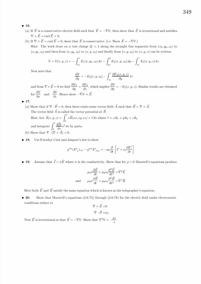
8/6/2019 Introduction to Tensor Calculus Continuum Mechanics - J. Heinbockel
http://slidepdf.com/reader/full/introduction-to-tensor-calculus-continuum-mechanics-j-heinbockel 355/372
34
16.
(a) If E is a conservative electric field such that E = −∇V , then show that E is irrotational and satisfies
∇ × E = curl E = 0.
(b) If ∇ × E = curl E = 0, show that E is conservative. (i.e. Show E = −∇V .)Hint: The work done on a test charge Q = 1 along the straight line segments from (x0, y0, z0) to
(x, y0, z0) and then from (x, y0, z0) to (x, y, z0) and finally from (x, y, z0) to (x, y, z) can be written
V = V (x, y, z) = − xx0
E 1(x, y0, z0) dx − yy0
E 2(x, y, z0) dy − zz0
E 3(x, y, z) dz.
Now note that∂ V ∂y
= −E 2(x, y, z0) − zz0
∂E 3(x, y, z)
∂ydz
and from ∇× E = 0 we find∂E 3∂y
=∂E 2∂z
, which implies∂ V ∂y
= −E 2(x, y, z). Similar results are obtained
for∂ V ∂x
and∂ V ∂z
. Hence show −∇V = E.
17.
(a) Show that if ∇ · B = 0, then there exists some vector field A such that B = ∇ × A.
The vector field A is called the vector potential of B.
Hint: Let A(x, y, z) =
10
s B(sx,sy,sz) × r ds where r = x e1 + y e2 + z e3and integrate
10
dBi
dss2 ds by parts.
(b) Show that ∇ · (∇ × A) = 0.
18. Use Faraday’s law and Ampere’s law to show
gim(E j,j),m − gjmE i,mj = −µ0∂
∂t J i + 0∂E i
∂t 19. Assume that J = σ E where σ is the conductivity. Show that for ρ = 0 Maxwell’s equations produce
µ0σ∂ E
∂t+ µ00
∂ 2 E
∂t2=∇2 E
and µ0σ∂ B
∂t+ µ00
∂ 2 B
∂t2=∇2 B.
Here both E and B satisfy the same equation which is known as the telegrapher’s equation.
20. Show that Maxwell’s equations (2.6.75) through (2.6.78) for the electric field under electrostaticconditions reduce to
∇ × E =0
∇ · D =ρf
Now E is irrotational so that E = −∇V . Show that ∇2V = −ρf
.

8/6/2019 Introduction to Tensor Calculus Continuum Mechanics - J. Heinbockel
http://slidepdf.com/reader/full/introduction-to-tensor-calculus-continuum-mechanics-j-heinbockel 356/372

8/6/2019 Introduction to Tensor Calculus Continuum Mechanics - J. Heinbockel
http://slidepdf.com/reader/full/introduction-to-tensor-calculus-continuum-mechanics-j-heinbockel 357/372
35
25. In a vacuum show that E and B satisfy
∇2 E =1
c2∂ 2 E
∂t2∇2 B =
1
c2∂ 2 B
∂t2∇ · E = 0 ∇ B = 0
26.
(a) Show that the wave equations in problem 25 have solutions in the form of waves traveling in thex- direction given by
E = E (x, t) = E 0ei(kx±ωt) and B = B(x, t) = B0ei(kx±ωt)
where E 0 and B0 are constants. Note that wave functions of the form u = Aei(kx±ωt) are called plane
harmonic waves. Sometimes they are called monochromatic waves. Here i2 = −1 is an imaginary unit.
Euler’s identity shows that the real and imaginary parts of these type wave functions have the form
A cos(kx ± ωt) and A sin(kx ± ωt).
These represent plane waves. The constant A is the amplitude of the wave , ω is the angular frequency,
and k/2π is called the wave number. The motion is a simple harmonic motion both in time and space.That is, at a fixed point x the motion is simple harmonic in time and at a fixed time t, the motion is
harmonic in space. By examining each term in the sine and cosine terms we find that x has dimensions of
length, k has dimension of reciprocal length, t has dimensions of time and ω has dimensions of reciprocal
time or angular velocity. The quantity c = ω/k is the wave velocity. The value λ = 2π/k has dimension
of length and is called the wavelength and 1/λ is called the wave number. The wave number represents
the number of waves per unit of distance along the x-axis. The period of the wave is T = λ/c = 2π/ω
and the frequency is f = 1/T. The frequency represents the number of waves which pass a fixed point
in a unit of time.
(b) Show that ω = 2πf
(c) Show that c = f λ
(d) Is the wave motion u = sin(kx − ωt) + sin(kx + ωt) a traveling wave? Explain.
(e) Show that in general the wave equation ∇2φ =1
c2∂ 2φ
∂t2have solutions in the form of waves traveling in
either the +x or −x direction given by
φ = φ(x, t) = f (x + ct) + g(x − ct)
where f and g are arbitrary twice differentiable functions.
(f) Assume a plane electromagnetic wave is moving in the +x direction. Show that the electric field is in
the xy−plane and the magnetic field is in the xz−plane.
Hint: Assume solutions E x = g1(x − ct), E y = g2(x − ct), E z = g3(x − ct), Bx = g4(x − ct),By = g5(x − ct), Bz = g6(x − ct) where gi,i = 1, ..., 6 are arbitrary functions. Then show that E x
does not satisfy ∇ · E = 0 which implies g1 must be independent of x and so not a wave function. Do
the same for the components of B. Since both ∇ · E = ∇ · B = 0 then E x = Bx = 0. Such waves
are called transverse waves because the electric and magnetic fields are perpendicular to the direction
of propagation. Faraday’s law implies that the E and B waves must be in phase and be mutually
perpendicular to each other.
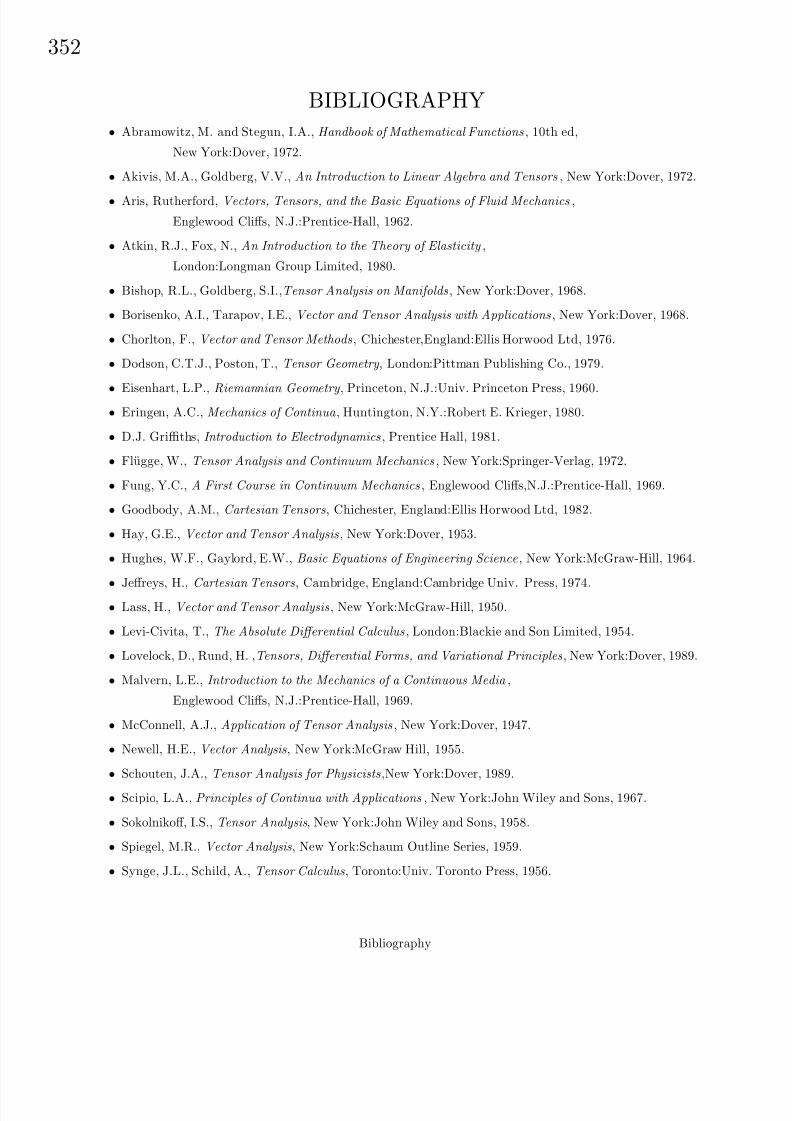
8/6/2019 Introduction to Tensor Calculus Continuum Mechanics - J. Heinbockel
http://slidepdf.com/reader/full/introduction-to-tensor-calculus-continuum-mechanics-j-heinbockel 358/372
352
BIBLIOGRAPHY
• Abramowitz, M. and Stegun, I.A., Handbook of Mathematical Functions, 10th ed,
New York:Dover, 1972.
• Akivis, M.A., Goldberg, V.V., An Introduction to Linear Algebra and Tensors, New York:Dover, 1972.
• Aris, Rutherford, Vectors, Tensors, and the Basic Equations of Fluid Mechanics,
Englewood Cliffs, N.J.:Prentice-Hall, 1962.
• Atkin, R.J., Fox, N., An Introduction to the Theory of Elasticity ,
London:Longman Group Limited, 1980.
• Bishop, R.L., Goldberg, S.I.,Tensor Analysis on Manifolds, New York:Dover, 1968.
• Borisenko, A.I., Tarapov, I.E., Vector and Tensor Analysis with Applications, New York:Dover, 1968.
• Chorlton, F., Vector and Tensor Methods, Chichester,England:Ellis Horwood Ltd, 1976.
• Dodson, C.T.J., Poston, T., Tensor Geometry , London:Pittman Publishing Co., 1979.
• Eisenhart, L.P., Riemannian Geometry , Princeton, N.J.:Univ. Princeton Press, 1960.• Eringen, A.C., Mechanics of Continua , Huntington, N.Y.:Robert E. Krieger, 1980.
• D.J. Griffiths, Introduction to Electrodynamics, Prentice Hall, 1981.
• Flugge, W., Tensor Analysis and Continuum Mechanics, New York:Springer-Verlag, 1972.
• Fung, Y.C., A First Course in Continuum Mechanics, Englewood Cliffs,N.J.:Prentice-Hall, 1969.
• Goodbody, A.M., Cartesian Tensors, Chichester, England:Ellis Horwood Ltd, 1982.
• Hay, G.E., Vector and Tensor Analysis, New York:Dover, 1953.
• Hughes, W.F., Gaylord, E.W., Basic Equations of Engineering Science, New York:McGraw-Hill, 1964.
• Jeffreys, H., Cartesian Tensors, Cambridge, England:Cambridge Univ. Press, 1974.• Lass, H., Vector and Tensor Analysis, New York:McGraw-Hill, 1950.
• Levi-Civita, T., The Absolute Differential Calculus, London:Blackie and Son Limited, 1954.
• Lovelock, D., Rund, H. ,Tensors, Differential Forms, and Variational Principles, New York:Dover, 1989.
• Malvern, L.E., Introduction to the Mechanics of a Continuous Media ,
Englewood Cliffs, N.J.:Prentice-Hall, 1969.
• McConnell, A.J., Application of Tensor Analysis, New York:Dover, 1947.
• Newell, H.E., Vector Analysis, New York:McGraw Hill, 1955.
• Schouten, J.A., Tensor Analysis for Physicists,New York:Dover, 1989.
• Scipio, L.A., Principles of Continua with Applications, New York:John Wiley and Sons, 1967.
• Sokolnikoff, I.S., Tensor Analysis, New York:John Wiley and Sons, 1958.
• Spiegel, M.R., Vector Analysis, New York:Schaum Outline Series, 1959.
• Synge, J.L., Schild, A., Tensor Calculus, Toronto:Univ. Toronto Press, 1956.
Bibliography
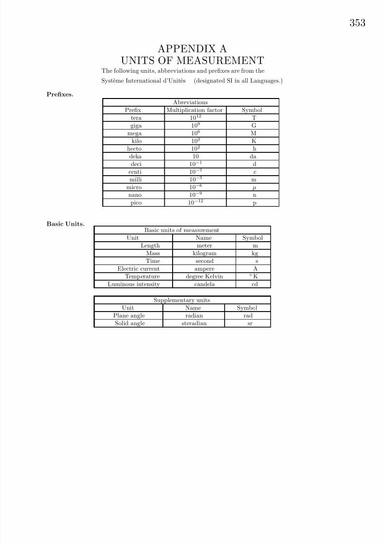
8/6/2019 Introduction to Tensor Calculus Continuum Mechanics - J. Heinbockel
http://slidepdf.com/reader/full/introduction-to-tensor-calculus-continuum-mechanics-j-heinbockel 359/372
35
APPENDIX AUNITS OF MEASUREMENT
The following units, abbreviations and prefixes are from the
Systeme International d’Unites (designated SI in all Languages.)
Prefixes.Abreviations
Prefix Multiplication factor Symboltera 1012 Tgiga 109 G
mega 106 Mkilo 103 K
hecto 102 hdeka 10 dadeci 10−1 d
centi 10−2 cmilli 10−3 m
micro 10
−6
µnano 10−9 npico 10−12 p
Basic Units.Basic units of measurement
Unit Name SymbolLength meter m
Mass kilogram kgTime second s
Electric current ampere ATemperature degree Kelvin K
Luminous intensity candela cd
Supplementary unitsUnit Name Symbol
Plane angle radian radSolid angle steradian sr

8/6/2019 Introduction to Tensor Calculus Continuum Mechanics - J. Heinbockel
http://slidepdf.com/reader/full/introduction-to-tensor-calculus-continuum-mechanics-j-heinbockel 360/372
354
DERIVED UNITSName Units Symbol
Area square meter m2
Volume cubic meter m3
Frequency hertz Hz (s−1)Density kilogram per cubic meter kg/m3
Velocity meter per second m/sAngular velocity radian per second rad/s
Acceleration meter per second squared m/s2
Angular acceleration radian per second squared rad/s2
Force newton N (kg · m/s2)Pressure newton per square meter N/m2
Kinematic viscosity square meter per second m2/sDynamic viscosity newton second per square meter N · s/m2
Work, energy, quantity of heat joule J (N ·m)Power watt W (J/s)
Electric charge coulomb C (A · s)Voltage, Potential difference volt V (W/A)
Electromotive force volt V (W/A)Electric force field volt per meter V/mElectric resistance ohm Ω (V/A)
Electric capacitance farad F (A · s/V)Magnetic flux weber Wb (V · s)
Inductance henry H (V · s/A)Magnetic flux density tesla T (Wb/m2)
Magnetic field strength ampere per meter A/mMagnetomotive force ampere A
Physical constants.
4 arctan1 = π = 3.14159 26535 89793 23846 2643 . . .
limn→∞
1 +
1
n
n
= e = 2.71828 18284 59045 23536 0287 . . .
Euler’s constant γ = 0.57721 56649 01532 86060 6512 . . .
γ = limn→∞
1 +
1
2+
1
3+ · · · +
1
n− log n
speed of light in vacuum = 2.997925(10)8 m s−1
electron charge = 1.60210(10)−19 C
Avogadro’s constant = 6.02252(10)23 mol−1
Plank’s constant = 6.6256(10)−34
J s
Universal gas constant = 8.3143 J K −1 mol−1 = 8314.3 J Kg−1 K −1
Boltzmann constant = 1.38054(10)−23 J K −1
Stefan–Boltzmann constant = 5.6697(10)−8 W m−2 K −4
Gravitational constant = 6.67(10)−11 N m2kg−2

8/6/2019 Introduction to Tensor Calculus Continuum Mechanics - J. Heinbockel
http://slidepdf.com/reader/full/introduction-to-tensor-calculus-continuum-mechanics-j-heinbockel 361/372
35
APPENDIX BCHRISTOFFEL SYMBOLS OF SECOND KIND
1. Cylindrical coordinates (r,θ,z) = (x1, x2, x3)
x = r cos θ
y = r sin θ
z = z
r ≥ 0
0 ≤ θ ≤ 2π
−∞ < z < ∞
h1 = 1
h2 = r
h3 = 1
The coordinate curves are formed by the intersection of the coordinate surfaces
x2 + y2 = r2, Cylinders
y/x = tan θ Planes
z = Constant Planes.
1
2 2
= −r
2
1 2
=
2
2 1
=
1
r
2. Spherical coordinates (ρ,θ,φ) = (x1, x2, x3)
x = ρ sin θ cos φ
y = ρ sin θ sin φ
z = ρ cos θ
ρ ≥ 0
0 ≤ θ ≤ π
0 ≤ φ ≤ 2π
h1 = 1
h2 = ρ
h3 = ρ sin θ
The coordinate curves are formed by the intersection of the coordinate surfaces
x2 + y2 + z2 = ρ2 Spheres
x2 + y2 = tan2 θ z Cones
y = x tan φ Planes.
1
2 2
= −ρ
1
3 3
= −ρ sin2 θ
2
3 3
= − sin θ cos θ
2
1 2
=
2
2 1
=
1
ρ3
1 3
=
3
3 1
=
1
ρ3
3 2
=
3
2 3
= cot θ
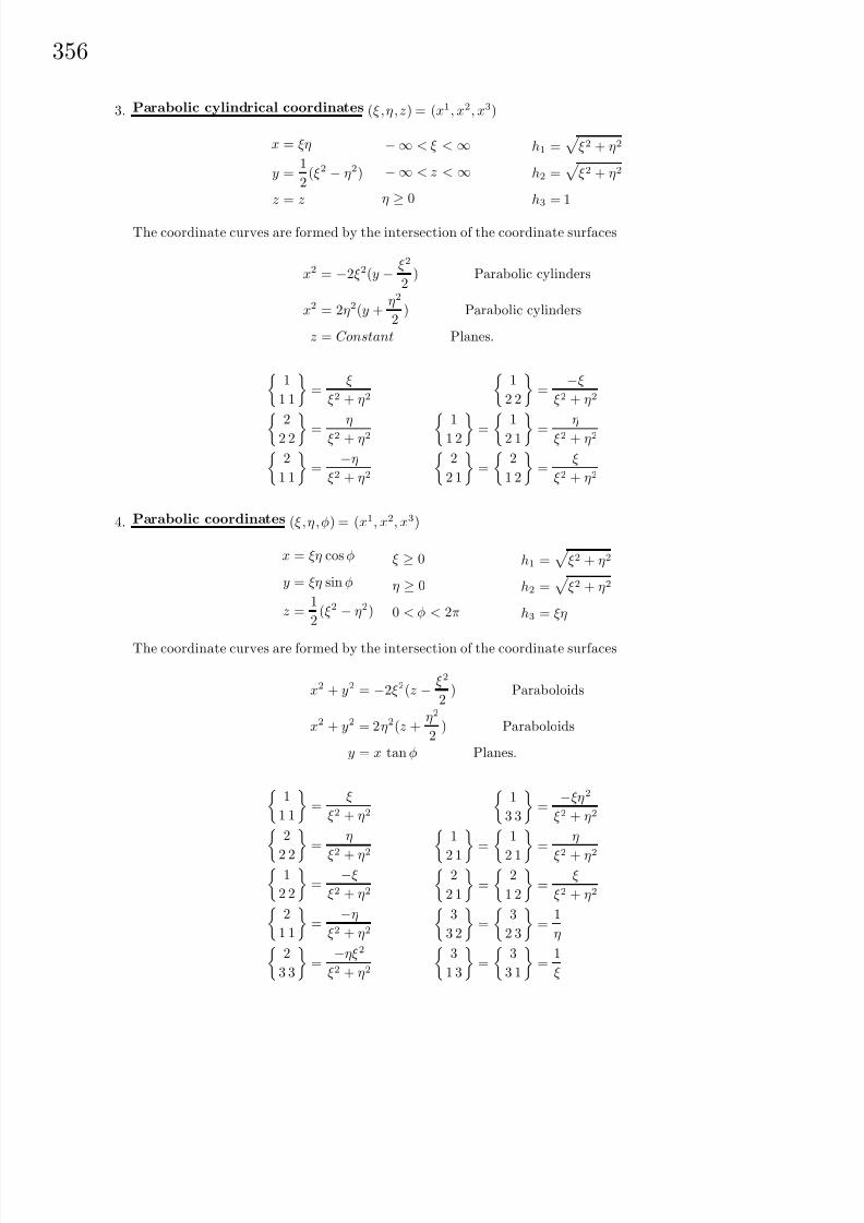
8/6/2019 Introduction to Tensor Calculus Continuum Mechanics - J. Heinbockel
http://slidepdf.com/reader/full/introduction-to-tensor-calculus-continuum-mechanics-j-heinbockel 362/372
356
3. Parabolic cylindrical coordinates (ξ, η, z) = (x1, x2, x3)
x = ξη
y =1
2(ξ2 − η2)
z = z
−∞ < ξ < ∞
−∞ < z < ∞
η ≥ 0
h1 =
ξ2 + η2
h2 =
ξ2 + η2
h3 = 1
The coordinate curves are formed by the intersection of the coordinate surfaces
x2 = −2ξ2(y −ξ2
2) Parabolic cylinders
x2 = 2η2(y +η2
2) Parabolic cylinders
z = Constant Planes.
1
1 1
=
ξ
ξ2 + η2
2
2 2
=η
ξ2 + η22
1 1
=
−η
ξ2 + η2
1
2 2
=
−ξ
ξ2 + η2
1
1 2
= 1
2 1
=η
ξ2 + η22
2 1
=
2
1 2
=
ξ
ξ2 + η2
4. Parabolic coordinates (ξ, η, φ) = (x1, x2, x3)
x = ξη cos φ
y = ξη sin φ
z =1
2(ξ2 − η2)
ξ ≥ 0
η ≥ 0
0 < φ < 2π
h1 =
ξ2 + η2
h2 =
ξ2 + η2
h3 = ξη
The coordinate curves are formed by the intersection of the coordinate surfaces
x2 + y2 = −2ξ2(z −ξ2
2) Paraboloids
x2 + y2 = 2η2(z +η2
2) Paraboloids
y = x tan φ Planes.
1
1 1
=
ξ
ξ2 + η2
2
2 2 =
η
ξ2
+ η2
1
2 2
=
−ξ
ξ2 + η22
1 1
=
−η
ξ2 + η22
3 3
=
−ηξ2
ξ2 + η2
1
3 3
=
−ξη2
ξ2 + η2
1
2 1 = 1
2 1 =
η
ξ2
+ η2
2
2 1
=
2
1 2
=
ξ
ξ2 + η23
3 2
=
3
2 3
=
1
η3
1 3
=
3
3 1
=
1
ξ

8/6/2019 Introduction to Tensor Calculus Continuum Mechanics - J. Heinbockel
http://slidepdf.com/reader/full/introduction-to-tensor-calculus-continuum-mechanics-j-heinbockel 363/372
35
5. Elliptic cylindrical coordinates (ξ, η, z) = (x1, x2, x3)
x = cosh ξ cos η
y = sinh ξ sin η
z = z
ξ ≥ 0
0 ≤ η ≤ 2π
−∞ < z < ∞
h1 =
sinh2 ξ + sin2 η
h2 =
sinh2 ξ + sin2 η
h3 = 1
The coordinate curves are formed by the intersection of the coordinate surfaces
x2
cosh2 ξ+
y2
sinh2 ξ= 1 Elliptic cylinders
x2
cos2 η−
y2
sin2 η= 1 Hyperbolic cylinders
z = Constant Planes.
1
1 1
=
sinh ξ cosh ξ
sinh2 ξ + sin2 η
1
2 2
=
− sinh ξ cosh ξ
sinh2 ξ + sin2 η1
1 2
=
1
2 1
=
sin η cos η
sinh2 ξ + sin2 η
2
2 2
=
sin η cos η
sinh2 ξ + sin2 η
2
1 1
=
− sin η cos η
sinh2 ξ + sin2 η2
1 2
=
2
2 1
=
sinh ξ cosh ξ
sinh2 ξ + sin2 η
6. Elliptic coordinates (ξ, η, φ) = (x1, x2, x3)
x =
(1− η2)(ξ2 − 1)cos φ
y =
(1− η2)(ξ2 − 1)sin φ
z = ξη
1 ≤ ξ < ∞
− 1 ≤ η ≤ 1
0 ≤ φ < 2π
h1 =
ξ2 − η2
ξ2 − 1
h2 =
ξ2 − η2
1 − η2
h3
=
(1 − η2
)(ξ2
− 1)The coordinate curves are formed by the intersection of the coordinate surfaces
x2
ξ2 − 1+
y2
ξ2 − 1+
z2
ξ2= 1 Prolate ellipsoid
z2
η2−
x2
1 − η2−
y2
1 − η2= 1 Two-sheeted hyperboloid
y = x tan φ Planes
1
1 1
= −
ξ
−1 + ξ2+
ξ
ξ2 − η2
2
2 2
=
η
1 − η2 −
η
ξ2 − η21
2 2
= −
ξ−1 + ξ2
(1 − η2) (ξ2 − η2)
1
3 3
= −
ξ−1 + ξ2
1 − η2
ξ2 − η2
2
1 1
=
η
1 − η2
(−1 + ξ2) (ξ2 − η2)
2
3 3
=
−1 + ξ2
η
1 − η2
ξ2 − η2
1
1 2
= −η
ξ2 − η22
2 1
=
ξ
ξ2 − η23
3 1
=
ξ
−1 + ξ23
3 2
= −
η
1− η2
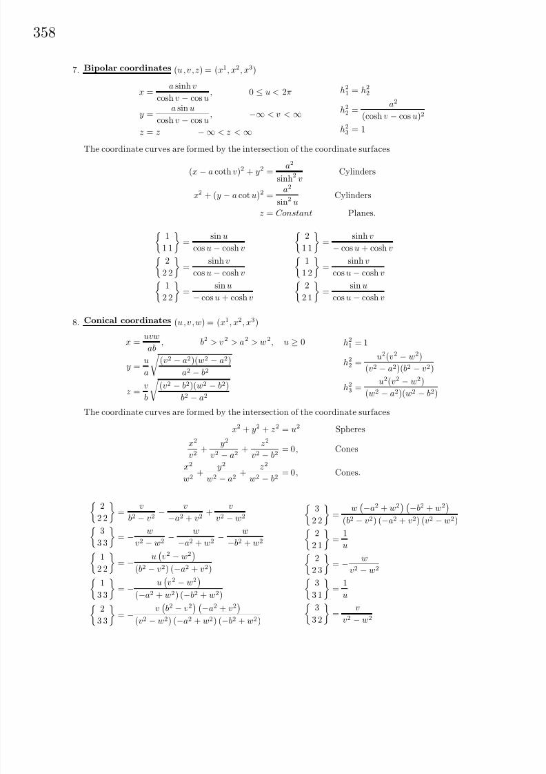
8/6/2019 Introduction to Tensor Calculus Continuum Mechanics - J. Heinbockel
http://slidepdf.com/reader/full/introduction-to-tensor-calculus-continuum-mechanics-j-heinbockel 364/372
358
7. Bipolar coordinates (u, v, z) = (x1, x2, x3)
x =a sinh v
cosh v − cos u, 0 ≤ u < 2π
y =a sin u
cosh v − cos u, −∞ < v < ∞
z = z −∞ < z < ∞
h2
1 = h2
2
h2
2 =a2
(cosh v − cos u)2
h2
3= 1
The coordinate curves are formed by the intersection of the coordinate surfaces
(x − a coth v)2 + y2 =a2
sinh2 vCylinders
x2 + (y − a cot u)2 =a2
sin2 uCylinders
z = Constant Planes.
1
1 1
=
sin u
cos u− cosh v
2
2 2
=
sinh v
cos u− cosh v1
2 2
=
sin u
− cos u + cosh v
2
1 1
=
sinh v
− cos u + cosh v
1
1 2
=
sinh v
cos u− cosh v2
2 1
=
sin u
cos u− cosh v
8. Conical coordinates (u, v, w) = (x1, x2, x3)
x =uvw
ab, b2 > v2 > a2 > w2, u ≥ 0
y =u
a
(v2 − a2)(w2 − a2)
a2 − b2
z =v
b
(v2 − b2)(w2 − b2)
b2 − a2
h2
1 = 1
h2
2 =u2(v2 − w2)
(v2 − a2)(b2 − v2)
h2
3=
u2(v2 − w2)
(w2 − a2)(w2 − b2)
The coordinate curves are formed by the intersection of the coordinate surfaces
x2 + y2 + z2 = u2 Spheres
x2
v2+
y2
v2 − a2+
z2
v2 − b2= 0, Cones
x2
w2+
y2
w2 − a2+
z2
w2 − b2= 0, Cones.
2
2 2
=
v
b2 − v2−
v
−a2 + v2+
v
v2 −w2
3
3 3 = −
w
v2 −w2
−w
−a2 + w2
−w
−b2 + w21
2 2
= −
u
v2 −w2
(b2 − v2) (−a2 + v2)1
3 3
= −
u
v2 −w2
(−a2 + w2) (−b2 + w2)2
3 3
= −
v
b2 − v2 −a2 + v2
(v2 −w2) (−a2 + w2) (−b2 + w2)
3
2 2
=
w−a2 + w2
−b2 + w2
(b2 − v2) (−a2 + v2) (v2 −w2)
2
2 1
=
1
u2
2 3
= −
w
v2 − w23
3 1
=
1
u3
3 2
=
v
v2 −w2

8/6/2019 Introduction to Tensor Calculus Continuum Mechanics - J. Heinbockel
http://slidepdf.com/reader/full/introduction-to-tensor-calculus-continuum-mechanics-j-heinbockel 365/372
35
9. Prolate spheroidal coordinates (u, v, φ) = (x1, x2, x3)
x = a sinh u sin v cos φ, u ≥ 0
y = a sinh u sin v sin φ, 0 ≤ v ≤ π
z = a cosh u cos v, 0 ≤ φ < 2π
h2
1= h2
2
h2
2= a2(sinh2 u + sin2 v)
h2
3 = a2 sinh2 u sin2 v
The coordinate curves are formed by the intersection of the coordinate surfacesx2
(a sinh u)2+
y2
a sinh u)2+
z2
a cosh u)2= 1, Prolate ellipsoids
x2
(a cos v)2−
y2
(a sin v)2−
z2
(a cos v)2= 1, Two-sheeted hyperpoloid
y = x tan φ, Planes.
1
1 1
=
cosh u sinh u
sin2 v + sinh2 u2
2 2
=
cos v sin v
sin2 v + sinh2 u1
2 2
= − cosh u sinh u
sin2 v + sinh2 u1
3 3
= −
sin2 v cosh u sinh u
sin2 v + sinh2 u2
1 1
= −
cos v sin v
sin2 v + sinh2 u
2
3 3
= −
cos v sin vsinh2 u
sin2 v + sinh2 u1
1 2
=
cos v sin v
sin2 v + sinh2 u2
2 1
= cosh u sinh u
sin2 v + sinh2 u3
3 1
=
cosh u
sinh u3
3 2
=
cos v
sin v
10. Oblate spheroidal coordinates (ξ, η, φ) = (x1, x2, x3)
x = a cosh ξ cos η cos φ, ξ ≥ 0
y = a cosh ξ cos η sin φ, −π
2≤ η ≤
π
2
z = a sinh ξ sin η, 0 ≤ φ ≤ 2π
h2
1 = h2
2
h2
2 = a2(sinh2 ξ + sin2 η)
h23 = a2 cosh2
ξ cos2 η
The coordinate curves are formed by the intersection of the coordinate surfaces
x2
(a cosh ξ)2+
y2
(a cosh ξ)2+
z2
(a sinh ξ)2= 1, Oblate ellipsoids
x2
(a cos η)2+
y2
(a cos η)2−
z2
(a sin η)2= 1, One-sheet hyperboloids
y = x tan φ, Planes.
1
1 1
=
cosh ξ sinh ξ
sin2 η + sinh2 ξ
2
2 2
=cos η sin η
sin2 η + sinh2 ξ1
2 2
= −
cosh ξ sinh ξ
sin2 η + sinh2 ξ1
3 3
= −
cos2 η cosh ξ sinh ξ
sin2 η + sinh2 ξ2
1 1
= −
cos η sin η
sin2 η + sinh2 ξ
2
3 3
=
cos η sin ηcosh2 ξ
sin2 η + sinh2 ξ
1
1 2
=cos η sin η
sin2 η + sinh2 ξ2
2 1
=
cosh ξ sinh ξ
sin2 η + sinh2 ξ3
3 1
=
sinh ξ
cosh ξ3
3 2
= −
sin η
cos η

8/6/2019 Introduction to Tensor Calculus Continuum Mechanics - J. Heinbockel
http://slidepdf.com/reader/full/introduction-to-tensor-calculus-continuum-mechanics-j-heinbockel 366/372
360
11. Toroidal coordinates (u, v, φ) = (x1, x2, x3)
x =a sinh v cos φ
cosh v − cos u, 0 ≤ u < 2π
y =a sinh v sin φ
cosh v − cos u, −∞ < v < ∞
z = a sin ucosh v − cos u
, 0 ≤ φ < 2π
h2
1 = h2
2
h2
2 =a2
(cosh v − cos u)2
h23 = a
2
sinh
2
v(cosh v − cos u)2
The coordinate curves are formed by the intersection of the coordinate surfaces
x2 + y2 +
z −a cos u
sin u
2=
a2
sin2 u, Spheres
x2 + y2 − acosh v
sinh v
2
+ z2 =a2
sinh2 v, Tores
y = x tan φ, planes
1
1 1
=
sin u
cos u − cosh v2
2 2
=
sinh v
cos u − cosh v1
2 2
=
sin u
− cos u + cosh v1
3 3
=
sin usinh v2
− cos u + cosh v2
1 1
=
sinh v
− cos u + cosh v
2
3 3
= −
sinh v (cos u cosh v − 1)
cos u − cosh v1
1 2
=
sinh v
cos u− cosh v2
2 1
=
sin u
cos u− cosh v3
3 1
=
sin u
cos u− cosh v3
3 2
=
cos u cosh v − 1
cos u sinh v − cosh v sinh v

8/6/2019 Introduction to Tensor Calculus Continuum Mechanics - J. Heinbockel
http://slidepdf.com/reader/full/introduction-to-tensor-calculus-continuum-mechanics-j-heinbockel 367/372
36
12. Confocal ellipsoidal coordinates (u, v, w) = (x1, x2, x3)
x2 =(a2 − u)(a2 − v)(a2 −w)
(a2 − b2)(a2 − c2), u < c2 < b2 < a2
y2 =(b2 − u)(b2 − v)(b2 −w)
(b2 − a2)(b2 − c2), c2 < v < b2 < a2
z2 =(c2 − u)(c2 − v)(c2 −w)
(c2 − a2)(c2 − b2), c2 < b2 < v < a2
h2
1 =(u− v)(u − w)
4(a2 − u)(b2 − u)(c2 − u)
h2
2=
(v − u)(v − w)
4(a2 − v)(b2 − v)(c2 − v)
h2
3 =(w − u)(w − v)
4(a2 − w)(b2 − w)(c2 −w)
1
1 1
=
1
2 (a2 − u) +
1
2 (b2 − u) +
1
2 (c2 − u) +
1
2 (u − v) +
1
2 (u −w)2
2 2
=
1
2 (a2 − v)+
1
2 (b2 − v)+
1
2 (c2 − v)+
1
2 (−u + v)+
1
2 (v −w)3
3 3
=
1
2 (a2 −w)+
1
2 (b2 − w)+
1
2 (c2 −w)+
1
2 (−u + w)+
1
2 (−v + w)1
2 2
=
a2 − u
b2 − u
c2 − u
(v −w)
2 (a2 − v) (b2 − v) (c2 − v) (u− v) (u− w)1
3 3
=
a2 − u
b2 − u
c2 − u
(−v + w)
2 (u− v) (a2 −w) (b2 −w) (c2 − w) (u −w)
2
1 1 = a2 − v b2 − v c2 − v (u −w)
2 (a2
− u) (b2
− u) (c2
− u) (−u + v) (v −w)2
3 3
=
a2 − v
b2 − v
c2 − v
(−u + w)
2 (−u + v) (a2 −w) (b2 − w) (c2 −w) (v −w)3
1 1
=
(u − v)
a2 −w
b2 − w
c2 −w
2 (a2 − u) (b2 − u) (c2 − u) (−u + w) (−v + w)3
2 2
=
(−u + v)
a2 −w
b2 − w
c2 −w
2 (a2 − v) (b2 − v) (c2 − v) (−u + w) (−v + w)
1
1 2
=
−1
2 (u − v)1
1 3
=
−1
2 (u −w)
2
2 1 =
−1
2 (−u + v)2
2 3
=
−1
2 (v − w)3
3 1
=
−1
2 (−u + w)3
3 2
=
−1
2 (−v + w)

8/6/2019 Introduction to Tensor Calculus Continuum Mechanics - J. Heinbockel
http://slidepdf.com/reader/full/introduction-to-tensor-calculus-continuum-mechanics-j-heinbockel 368/372
362
APPENDIX CVECTOR IDENTITIES
The following identities assume that A, B, C, D are differentiable vector functions of position while
f, f 1, f 2 are differentiable scalar functions of position.
1. A · ( B × C ) = B · ( C × A) = C · ( A× B)
2. A × ( B × C ) = B( A · C ) − C ( A · B)
3. ( A × B) · ( C × D) = ( A · C )( B · D)− ( A · D)( B · C )
4. A× ( B × C ) + B × ( C × A) + C × ( A × B) = 0
5. ( A × B) × ( C × D) = B( A · C × D) − A( B · C × D)
= C ( A · B × C )− D( A · B × C )
6. ( A× B) · ( B × C ) × ( C × A) = ( A · B × C )2
7. ∇(f 1 + f 2) = ∇f 1 +∇f 2
8. ∇ · ( A + B) = ∇ · A +∇ · B
9. ∇× ( A + B) = ∇× A + ∇× B
10. ∇(f A) = (∇f ) · A + f ∇ · A
11. ∇(f 1f 2) = f 1∇f 2 + f 2∇f 1
12. ∇× (f A) =)∇f )× A + f (∇× A)
13. ∇ · ( A × B) = B · (∇× A) − A · (∇× B)
14. ( A · ∇) A = ∇
| A|2
2
− A× (∇× A)
15. ∇( A · B) = ( B · ∇) A + ( A · ∇) B + B × (∇× A) + A × (∇× B)
16. ∇× ( A × B) = ( B · ∇) A− B(∇ · A)− ( A · ∇) B + A(∇ · B)
17. ∇ · (∇f ) = ∇2f
18. ∇× (∇f ) = 0
19. ∇ · (∇× A) = 0
20. ∇× (∇× A) = ∇(∇ · A) −∇2
A

8/6/2019 Introduction to Tensor Calculus Continuum Mechanics - J. Heinbockel
http://slidepdf.com/reader/full/introduction-to-tensor-calculus-continuum-mechanics-j-heinbockel 369/372
INDEX 363
A
Absolute differentiation 120
Absolute scalar field 43
Absolute tensor 45,46,47,48
Acceleration 121, 190, 192Action integral 198
Addition of systems 6, 51
Addition of tensors 6, 51
Adherence boundary condition 294
Aelotropic material 245
Affine transformation 86, 107
Airy stress function 264
Almansi strain tensor 229
Alternating tensor 6,7
Ampere’s law 176,301,337,341
Angle between vectors 80, 82
Angular momentum 218, 287
Angular velocity 86,87,201,203
Arc length 60, 67, 133
Associated tensors 79
Auxiliary Magnetic field 338
Axis of symmetry 247
B
Basic equations elasticity 236, 253, 270
Basic equations for a continuum 236
Basic equations of fluids 281, 287
Basis vectors 1,2,37,48
Beltrami 262
Bernoulli’s Theorem 292
Biharmonic equation 186, 265
Bilinear form 97
Binormal vector 130
Biot-Savart law 336
Bipolar coordinates 73
Boltzmann equation 302,306
Boundary conditions 257, 294
Bulk modulus 251
Bulk coefficient of viscosity 285
C
Cartesian coordinates 19,20,42, 67, 83
Cartesian tensors 84, 87, 226
Cauchy stress law 216
Cauchy-Riemann equations 293,321
Charge density 323
Christoffel symbols 108,110,111
Circulation 293
Codazzi equations 139
Coefficient of viscosity 285
Cofactors 25, 26, 32
Compatibility equations 259, 260, 262
Completely skew symmetric system 31
Compound pendulum 195,209
Compressible material 231
Conic sections 151
Conical coordinates 74Conjugate dyad 49
Conjugate metric tensor 36, 77
Conservation of angular momentum 218, 295
Conservation of energy 295
Conservation of linear momentum 217, 295
Conservation of mass 233, 295
Conservative system 191, 298
Conservative electric field 323
Constitutive equations 242, 251,281, 287
Continuity equation 106,234, 287, 335
Contraction 6, 52
Contravariant components 36, 44
Contravariant tensor 45
Coordinate curves 37, 67
Coordinate surfaces 37, 67
Coordinate transformations 37
Coulomb law 322
Covariant components 36, 47
Covariant differentiation 113,114,117
Covariant tensor 46
Cross product 11
Curl 21, 173
Curvature 130, 131, 134, 149
Curvature tensor 134, 145
Curvilinear coordinates 66, 81
Cylindrical coordinates 18, 42, 69

8/6/2019 Introduction to Tensor Calculus Continuum Mechanics - J. Heinbockel
http://slidepdf.com/reader/full/introduction-to-tensor-calculus-continuum-mechanics-j-heinbockel 370/372
364 INDEX
D
Deformation 222
Derivative of tensor 108
Derivatives and indicial notation 18, 31
Determinant 10, 25, 32, 33Dielectric tensor 333
Differential geometry 129
Diffusion equation 303
Dilatation 232
Direction cosines 85
Displacement vector 333
Dissipation function 297
Distribution function 302
Divergence 21, 172
Divergence theorem 24
Dot product 5
Double dot product 50, 62
Dual tensor 100
Dummy index 4, 5
Dyads 48,62,63
Dynamics 187
E
e Permutation symbol 6, 7, 12e-δ identity 12
Eigenvalues 179,189
Eigenvectors 179,186
Einstein tensor 156
Elastic constants 248
Elastic stiffness 242
Elasticity 211,213
Electrostatic field 322,333
Electric flux 327
Electric units 322
Electrodynamics 339
Electromagnetic energy 341
Electromagnetic stress 341,342
Elliptic coordinates 72
Elliptical cylindrical coordinates 71
Enthalpy 298
Entropy 300
Epsilon permutation symbol 83
Equation of state 300
Equilibrium equations 273,300
Elastic constants 243,248
Equipotential curves 325
Euler number 294
Euler-Lagrange equations 192
Eulerian angles 201, 209
Eulerian form 287
Eulerian system 227
Eulers equations of motion 204
F
Faraday’s law 176,301, 340
Field lines 324, 327
Field electric 322
First fundamental form 133,143
Fourier law 297, 299
Free indices 3
Frenet-Serret formulas 131, 188
Froude number 294
Fluids 281
G
Gas law 300Gauss divergence theorem 24, 330
Gauss equations 138
Gauss’s law for electricity 176,301,328
Gauss’s law for magnetism 176,301,341
Gaussian curvature 137,139, 149
Geodesics 140, 146
Geodesic curvature 135, 140
General tensor 48
Generalized e− δ identity 84, 104
Generalized Hooke’s law 242
Generalized Kronecker delta 13, 31
Generalized stress strain 242
Geometry in Riemannian Space 80
Gradient 20, 171
Gradient basis 37
Green’s theorem 24
Group properties 41, 54
Generalized velocity 121
Generalized acceleration 121

8/6/2019 Introduction to Tensor Calculus Continuum Mechanics - J. Heinbockel
http://slidepdf.com/reader/full/introduction-to-tensor-calculus-continuum-mechanics-j-heinbockel 371/372
INDEX 365
H
Hamiltonian 208
Heat equation 316
Hexagonal material 247
Higher order tensors 47, 93Hooke’s law 212, 242, 252
Hydrodynamic equations 283
I
Ideal fluid 283
Idemfactor 50
Incompressible material 231
Index notation 1, 2, 14
Indicial notation 1, 2, 14,24
Inner product 52
Inertia 30
Integral theorems 24
Intrinsic derivative 120
Invariant 43
Inviscid fluid 283
Isotropic material 248
Isotropic tensor 104
J
Jacobian 17, 30, 40, 101, 127
Jump discontinuity 330
K
Kronecker delta 3, 8, 13, 31, 76
Kinetic energy 201
Kinematic viscosity 302
L
Lagrange’s equation of motion 191, 196Lagrangian 209
Laplacian 174
Linear form 96
Linear momentum 209, 287
Linear transformation 86
Linear viscous fluids 284
Lorentz transformation 57
Lame’s constants 251
M
Magnitude of vector 80
Magnetostatics 334,338
Magnetic field 334
Magnetization vector 337
Magnetic permeability 337
Material derivative 234, 288
Material symmetry 244, 246
Maxwell equations 176, 339
Maxwell transfer equation 308
Maximum, minimum curvature 130, 140
Mean curvature 137, 148
Metric tensor 36, 65
Meusnier’s Theorem 150
Mixed tensor 49
Mohr’s circle 185
Moment of inertia 30, 184, 200
Momentum 217, 218
Multilinear forms 96, 98
Multiplication of tensors 6, 51
N
Navier’s equations 254, 257
Navier-Stokes equations 288, 290
Newtonian fluids 286
Nonviscous fluid 283
Normal curvature 135, 136
Normal plane 188
Normal stress 214
Normal vector 130, 132
Notation for physical components 92
O
Oblate Spheroidal coordinates 75
Oblique coordinates 60
Oblique cylindrical coordinates 102
Order 2
Orthogonal coordinates 78, 86
Orthotropic material 246
Outer product 6, 51
Osculating plane 188

8/6/2019 Introduction to Tensor Calculus Continuum Mechanics - J. Heinbockel
http://slidepdf.com/reader/full/introduction-to-tensor-calculus-continuum-mechanics-j-heinbockel 372/372
366 INDEX
P
Parallel vector field 122
Pappovich-Neuber solution 263
Parabolic coordinates 70
Parabolic cylindrical coordinates 69
Particle motion 190
Pendulum system 197, 210
Perfect gas 283, 299
Permutations 6
Phase space 302
Physical components 88, 91,93
Piezoelectric 300
Pitch,roll, Yaw 209
Plane Couette flow 315
Plane Poiseuille flow 316
Plane strain 263
Plane stress 264
Poisson’s equation 329
Poisson’s ratio 212
Polar element 273
Polarization vector 333
Polyads 48
Potential energy 191
Potential function 323Poynting’s vector 341
Pressure 283
Principal axes 183
Projection 35
Prolated Spheroidal coordinates 74
Pully system 194, 207
Q
Quotient law 53
R
Radius of curvature 130, 136
Rayleigh implusive flow 317
Reciprocal basis 35, 38
Relative scalar 127
Relative tensor 50, 121
Relative motion 202
Relativity 151
Relative motion 155
Reynolds number 294
Ricci’s theorem 119
Riemann Christoffel tensor 116, 129,139, 147
Riemann space 80
Rectifying plane 188
Rigid body rotation 199Rotation of axes 85, 87, 107
Rules for indices 2
S
Scalar 40, 43
Scalar invariant 43, 62, 105
Scalar potential 191
Scaled variables 293
Second fundamental form 135, 145Second order tensor 47
Shearing stresses 214
Simple pulley system 193
Simple pendulum 194
Skew symmetric system 3, 31
Skewed coordinates 60, 102
Solid angle 328
Space curves 130
Special tensors 65
Spherical coordinates 18, 43, 56, 69, 103,194
Stokes flow 318
Stokes hypothesis 285
Stokes theorem 24