A CONTINUUM MECHANICS APPROACH OF DERIVING STRESS TENSOR COMPONENTS OF DOUBLE SHEAR-PLANE REVOLUTE JOINTS IN THE ELASTIC DOMAIN

CHRISTOPHER STUBBS

A THESIS SUBMITTED TO THE GRADUATE

FACULTY OF RENSSELAER POLYTECHNIC INSTITUTE

IN PARTIAL FULFILLMENT OF THE

REQUIREMENTS FOR THE DEGREE OF

MASTER OF SCIENCE IN MECHANICAL ENGINEERING

INTRODUCTIONThe current engineering community uses finite element analyses in the development and design of double shear-plane clevis connections.

Although accurate, finite element analyses of this nature are:

• Non-linear in nature• Time consuming• Computationally intensive.

This thesis presents an approach for sizing frictionless double shear-plane clevis connections to be under their material yield strengths for their given application.

• Simple empirical formulae• No specialized personnel required to develop finite element models, • Shorter analysis time• Shorter iteration time to understand what dimensions and variables are

most critical for a given clevis system.

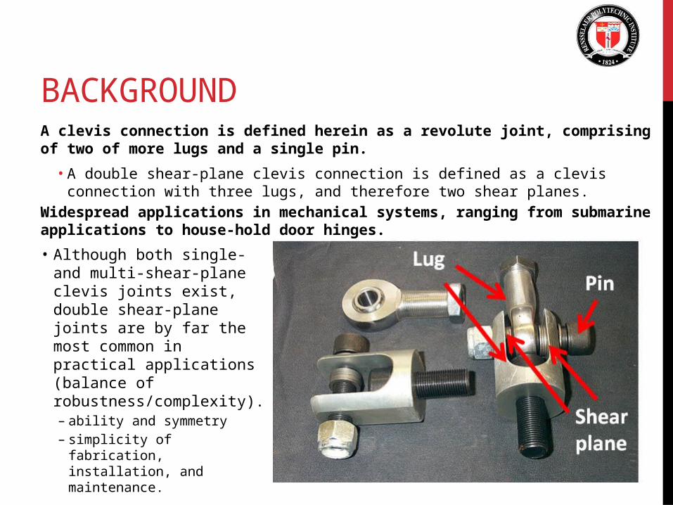
BACKGROUNDA clevis connection is defined herein as a revolute joint, comprising of two of more lugs and a single pin.

• A double shear-plane clevis connection is defined as a clevis connection with three lugs, and therefore two shear planes.

Widespread applications in mechanical systems, ranging from submarine applications to house-hold door hinges.

• Although both single- and multi-shear-plane clevis joints exist, double shear-plane joints are by far the most common in practical applications (balance of robustness/complexity). – ability and symmetry– simplicity of fabrication,

installation, and maintenance.

HISTORYCozzone & Melcon (1950): first to be able to correlate empirical data, destructive testing, and close-form formulae for predicting failure in the lug

Maddux (1953): evaluated both single shear and multi shear lug designs, for use in designing components to be under their ultimate strength

Rao (1978): evaluated the non-linearities of an initial clearance, and estimated the stresses in the pin, plate, and contact interface

Wearing (1985): used finite element analysis to transition from a pin within an infinite plate, to a pin within a clevis lug joint

Stenman (2008): re-evaluated Maddux’s conclusions for contact pressure

To (2008): evaluated conforming bushing designs

Antoni (2010): evaluated non-conforming bushing desings

Strozzi (2011): further investigated initial clearance

Kwon (2013): further investigated Maddux’s and Stenman’s findings on contact pressure

Leve

ragi

ng o

ff F

EA

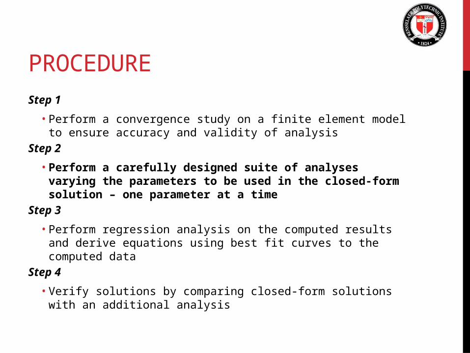
PROCEDUREStep 1

• Perform a convergence study on a finite element model to ensure accuracy and validity of analysis

Step 2

• Perform a carefully designed suite of analyses varying the parameters to be used in the closed-form solution – one parameter at a time

Step 3

• Perform regression analysis on the computed results and derive equations using best fit curves to the computed data

Step 4

• Verify solutions by comparing closed-form solutions with an additional analysis

STEP 1: CONVERGENCE STUDYA plot is produced of mesh density vs. stress, and then is normalized to the most dense mesh result.

von Mises stresses of the pin are within 10% accuracy with a mesh-radius ratio of 1, and within 5% accuracy with a mesh-radius ratio of 2

The von Mises stresses of the lug are within 10% accuracy with a mesh-radius ratio of 6, and within 5% accuracy with a mesh-radius ratio of 8

Therefore, a mesh-radius ratio of 8 is maintained throughout the study.

1 2 3 4 5 6 7 8 9 100.5

0.55

0.6

0.65

0.7

0.75

0.8

0.85

0.9

0.95

1

1.05

1.1

Pin Mises (S MISES)

Lug Mises (S MISES)

Shear Tear Out (S12)

Net Tensile (S22)

Pin Bending (S33)

Pin Shear (S12)

Lug Bearing (CPRESS)

Pin Bearing (CPRESS)

MR #

Val

ue

(No

rmal

ized

)

PROCEDUREStep 1

• Perform a convergence study on a finite element model to ensure accuracy and validity of analysis

Step 2

• Perform a carefully designed suite of analyses varying the parameters to be used in the closed-form solution – one parameter at a time

Step 3

• Perform regression analysis on the computed results and derive equations using best fit curves to the computed data

Step 4

• Verify solutions by comparing closed-form solutions with an additional analysis

STEP 2: MODEL DEVELOPMENT

The finite element model consists of:

• One-quarter pin• One-half outer lug• One-quarter middle lug

All elements are 3-dimensional 20-noded hexahedral reduced integration continuum elements, denoted in ABAQUS as C3D20R.

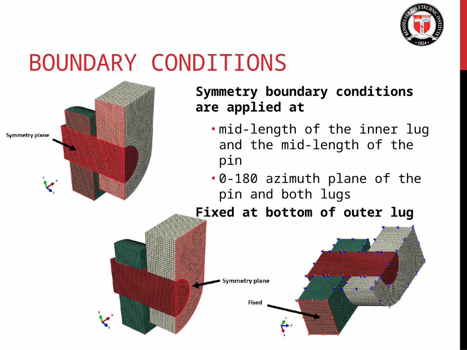
BOUNDARY CONDITIONSSymmetry boundary conditions are applied at

• mid-length of the inner lug and the mid-length of the pin

• 0-180 azimuth plane of the pin and both lugs

Fixed at bottom of outer lug

LOAD AND INTERACTIONSLoad is as a anti-pressure at the top of the inner lug

One contact interaction constraint is imposed in the model, between the pin and the lugs

• 3D surface smoothing• Instances are places in initial full-

closure• Normal contact: classical

Lagrange multiplier method• standard pressure-

overclosure relationship.

• Tangential contact: zero-penalty (frictionless / full-slip condition)

PARAMETRIC ANALYSES

Parametric UnitsMinimu

m Value

Maximu

m Value

Increment

Value

Analyses

Performed

Load lbf 400 4000 400 10

Lug Width in 0.5 2 0.25 7

Lug Gap in 0 0.9 0.1 10

Young's Modulus

of Pinpsi 1.00E+07 6.00E+07 1.00E+07 6

Poisson's Ratio

of Pin- 0.05 0.55 0.05 9

EXAMPLE OUTPUT

PROCEDUREStep 1

• Perform a convergence study on a finite element model to ensure accuracy and validity of analysis

Step 2

• Perform a carefully designed suite of analyses varying the parameters to be used in the closed-form solution – one parameter at a time

Step 3

• Perform regression analysis on the computed results and derive equations using best fit curves to the computed data

Step 4

• Verify solutions by comparing closed-form solutions with an additional analysis

REGRESSION ANALYSESThrough the use of regression analyses, multiplication factors are determined for each variable, and a final set of closed form expressions representing the finite element results are developed.

Equations are presented for von Mises stress in the lug, shear tear-out in the lug, contact pressure in the lug, von Mises stress in the pin, shear stress in the pin, and contact pressure in the pin.

For each stress mode, a general equation based upon the load applied is presented and then stress multiplication factors for each variable are presented.

• K1 is the multiplication factor from the axial gap between lugs

• K2 is the multiplication factor from the Young’s Moduli

• K3 is the multiplication factor from the Poisson’s ratios

• K4 is the multiplication factor from the lug width.

The equations were derived by creating a best fit curve for the data, evaluating them at the baseline condition (0.5” lug gap, 2” lug width, and Epin/Elug = Vpin/Vlug = 1), and dividing the equation by the result of the baseline equation, i.e. normalizing each equation such that at the baseline condition, the multiplication factor is equal to 1.

REGRESSION ANALYSES: EXAMPLEThe various analyses are post-process, and best-fit curves are created

The curves are created using a polynomial function of the power needed to create a good correlation (R2 > 0.98)

• The curve for load applied was set about a y-intercept of 0, as no stress exists with zero load applied

The equations taken from each curve, except for the load applied curve, are then evaluated for the baseline configuration

The equations are then normalized by their value at the baseline configuration.

• This is done to set each equation to 1.0 at the baseline configuration, such that the equations can be used as multiplication factors, or factors that affect the stress as a function of the system’s deviation from the baseline configuration.

REGRESSION ANALYSES: EXAMPLE

0.4 0.6 0.8 1 1.2 1.4 1.6 1.8 2 2.20

500

1000

1500

2000

2500

3000

f(x) = 636.44444444 x³ − 2914.4761905 x² + 4151.6984127 x + 541.85714286R² = 0.994448247397773

Lug von Mises vs.Lug Width (in)

Lug Mises (S MISES)

Polynomial (Lug Mises (S MISES))

0 0.1 0.2 0.3 0.4 0.5 0.6 0.7 0.8 0.9 10

500

1000

1500

2000

2500

3000

f(x) = 1279.69696969697 x + 1625.03636363636R² = 0.999583587574114

Lug von Mises vs.Lug Gap (in)

Lug Mises (S MISES)

Linear (Lug Mises (S MISES))

0.2 0.4 0.6 0.8 1 1.2 1.4 1.6 1.8 2 2.20

500

1000

1500

2000

2500

3000

3500

4000

f(x) = 580.982142857145 x² − 2377.25357142858 x + 4078.9R² = 0.995756269807145

Lug von Mises vs.Young’s Modulus Ratio (-)

Lug Mises (S MISES)

Polynomial (Lug Mises (S MISES))

0 0.2 0.4 0.6 0.8 1 1.2 1.4 1.62050

2100

2150

2200

2250

2300

2350

2400

f(x) = − 130.5 x + 2392.08333333333R² = 0.990914327607876

Lug von Mises vs.Poisson’s Ratio Ratio (-)

Lug Mises (S MISES)

Linear (Lug Mises (S MISES))

REGRESSION ANALYSES: EXAMPLE

REGRESSION ANALYSES: EXAMPLE

REGRESSION ANALYSES: EXAMPLE

These equations are then combined with the curve for the applied load, such that each multiplication factor is multiplied together, and then multiplied with the load applied curve.

This yields a final equation for von Mises stress in lug of:

0 1000 2000 3000 4000 50000

5000

10000

15000

20000

25000

f(x) = 5.86912987012987 xR² = 0.999999970139703

Lug Mises (S MISES)

Lug Mises (S MISES)

Linear (Lug Mises (S MISES))

PROCEDUREStep 1

• Perform a convergence study on a finite element model to ensure accuracy and validity of analysis

Step 2

• Perform a carefully designed suite of analyses varying the parameters to be used in the closed-form solution – one parameter at a time

Step 3

• Perform regression analysis on the computed results and derive equations using best fit curves to the computed data

Step 4

• Verify solutions by comparing closed-form solutions with an additional analysis

VERIFICATION ANALYSES

ParameterValue

Verification 1 Verification 2 Verification 3

Load (lbf) 400 800 80

Gap (in) 0.3 0.5 0.4

Epin (psi) 6.00E+07 4.00E+07 3.00E+07

Elug (psi) 3.00E+07 2.00E+07 3.00E+07

v_pin 0.15 0.3 0.2

v_lug 0.3 0.2 0.4

Lug Width

(in)1 1.4 1.2

VERIFICATION ANALYSES: EXAMPLEVerification 1 showed a maximum von Mises stress in the lug of 1612 psi

For that configuration, the computed multiplication factors, and computed von Mises stress is 1590 psi (1.36% Error)

VERIFICATION ANALYSESIt is found that the average error percentage among all stress components is less than 6.8%, within the acceptable limits of accuracy

Stress ComponentAverage Error

(%)

Lug von Mises 4.2

Lug shear tear-out 3.7

Lug contact pressure 5.7

Pin von Mises 6.8

Pin shear 1.4

Pin contact pressure 5.7

CONCLUSIONS

This thesis presented an approach for sizing frictionless double shear-plane clevis connections to be under their material yield strengths for their given application

Finite element analysis was utilized to simulate testing for purposes of developing empirical formulae based on the load through the connection, lug widths, lug gaps, Young’s moduli, and Poisson ratios

Regression analysis was then used to derive closed-form empirical formulae, using multiplication factors based upon each parametric evaluated

A verification analysis was performed to evaluate the error of the empirical formulae, and acceptable levels of accuracy were verified.

FUTURE WORK

This thesis laid the groundwork and approach that can be used in developing a closed-form solution for the full range of clevis connections

In this thesis, a number of stress components and a suite of variables were examined.

• This approach can be extended to study the effects of other variations on clevis connections, such as the existence of bearings, pin clearance, pin radius, and lug outer radius

• In addition, stress components such as pin bending and lug hoop stress can be evaluated further using this same technique.