Introduction to Statistical Learning and Machine...
74
Introduction to Statistical Learning and Machine Learning Chap 10 – Unsupervised Learning and Dimension Reduction Yanwei Fu School of Data Science, Fudan University 1/50
Transcript of Introduction to Statistical Learning and Machine...
Introduction to Statistical Learning and MachineLearning
Chap 10 – Unsupervised Learning and Dimension Reduction
Yanwei Fu
School of Data Science, Fudan University
1/50
1 Principal Components Analysis
2 ClusteringK-Meanshierarchical clustering
3 Gaussian Mixture Model (GMM)Mixtures of GaussiansExpectation Maximization (EM) Algorithm
2/50
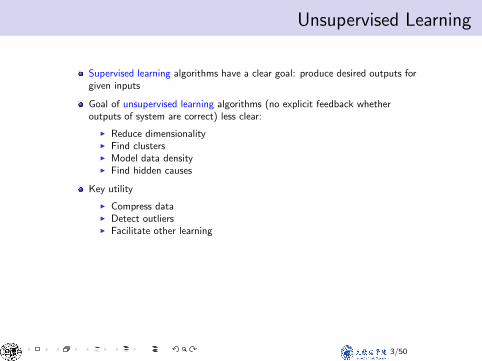
Unsupervised LearningUnsupervised Learning
Supervised learning algorithms have a clear goal: produce desired outputs forgiven inputs
Goal of unsupervised learning algorithms (no explicit feedback whetheroutputs of system are correct) less clear:
I Reduce dimensionalityI Find clustersI Model data densityI Find hidden causes
Key utility
I Compress dataI Detect outliersI Facilitate other learning
Urtasun & Zemel (UofT) CSC 411: 12-Clustering Oct 28, 2015 3 / 18
3/50
Unsupervised LearningUnsupervised Learning
Unsupervised vs Supervised Learning:
• Most of this course focuses on supervised learning methodssuch as regression and classification.
• In that setting we observe both a set of featuresX1, X2, . . . , Xp for each object, as well as a response oroutcome variable Y . The goal is then to predict Y usingX1, X2, . . . , Xp.
• Here we instead focus on unsupervised learning, we whereobserve only the features X1, X2, . . . , Xp. We are notinterested in prediction, because we do not have anassociated response variable Y .
1 / 52
3/50
The Goals of Unsupervised LearningMajor types
Primary problems, approaches in unsupervised learning fall into three classes:
1. Dimensionality reduction: represent each input case using a smallnumber of variables (e.g., principal components analysis, factoranalysis, independent components analysis)
2. Clustering: represent each input case using a prototype example (e.g.,k-means, mixture models)
3. Density estimation: estimating the probability distribution over thedata space
Urtasun & Zemel (UofT) CSC 411: 12-Clustering Oct 28, 2015 4 / 18
4/50

The Challenge of Unsupervised LearningThe Challenge of Unsupervised Learning
• Unsupervised learning is more subjective than supervisedlearning, as there is no simple goal for the analysis, such asprediction of a response.
• But techniques for unsupervised learning are of growingimportance in a number of fields:
• subgroups of breast cancer patients grouped by their geneexpression measurements,
• groups of shoppers characterized by their browsing andpurchase histories,
• movies grouped by the ratings assigned by movie viewers.
3 / 52
5/50
Another advantageAnother advantage
• It is often easier to obtain unlabeled data — from a labinstrument or a computer — than labeled data, which canrequire human intervention.
• For example it is difficult to automatically assess theoverall sentiment of a movie review: is it favorable or not?
4 / 52
6/50
Principal Components AnalysisPrincipal Components Analysis
• PCA produces a low-dimensional representation of adataset. It finds a sequence of linear combinations of thevariables that have maximal variance, and are mutuallyuncorrelated.
• Apart from producing derived variables for use insupervised learning problems, PCA also serves as a tool fordata visualization.
5 / 52
7/50
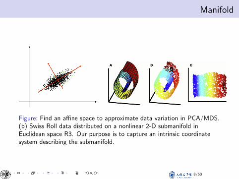
Manifold
Figure: Find an affine space to approximate data variation in PCA/MDS.(b) Swiss Roll data distributed on a nonlinear 2-D submanifold inEuclidean space R3. Our purpose is to capture an intrinsic coordinatesystem describing the submanifold.
8/50
Principal Components Analysis: detailsPrincipal Components Analysis: details
• The first principal component of a set of featuresX1, X2, . . . , Xp is the normalized linear combination of thefeatures
Z1 = φ11X1 + φ21X2 + . . .+ φp1Xp
that has the largest variance. By normalized, we mean that∑pj=1 φ
2j1 = 1.
• We refer to the elements φ11, . . . , φp1 as the loadings of thefirst principal component; together, the loadings make upthe principal component loading vector,φ1 = (φ11 φ21 . . . φp1)
T .
• We constrain the loadings so that their sum of squares isequal to one, since otherwise setting these elements to bearbitrarily large in absolute value could result in anarbitrarily large variance.
6 / 52
9/50
Principal Components Analysis: detailsPCA: example
10 20 30 40 50 60 70
05
10
15
20
25
30
35
Population
Ad
Sp
en
din
g
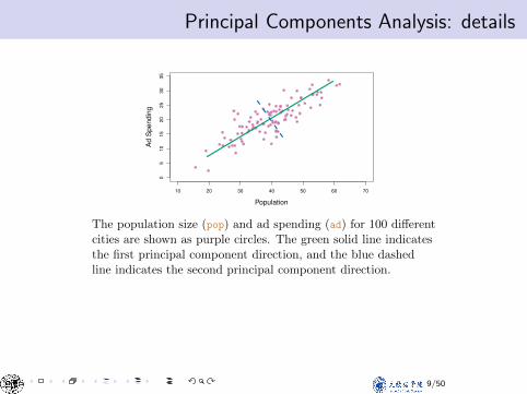
The population size (pop) and ad spending (ad) for 100 differentcities are shown as purple circles. The green solid line indicatesthe first principal component direction, and the blue dashedline indicates the second principal component direction.
7 / 52
9/50
Principal Components Analysis: detailsComputation of Principal Components
• Suppose we have a n× p data set X. Since we are onlyinterested in variance, we assume that each of the variablesin X has been centered to have mean zero (that is, thecolumn means of X are zero).
• We then look for the linear combination of the samplefeature values of the form
zi1 = φ11xi1 + φ21xi2 + . . .+ φp1xip (1)
for i = 1, . . . , n that has largest sample variance, subject tothe constraint that
∑pj=1 φ
2j1 = 1.
• Since each of the xij has mean zero, then so does zi1 (forany values of φj1). Hence the sample variance of the zi1can be written as 1
n
∑ni=1 z
2i1.
8 / 52
9/50
Principal Components Analysis: detailsComputation: continued
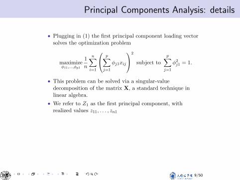
• Plugging in (1) the first principal component loading vectorsolves the optimization problem
maximizeφ11,...,φp1
1
n
n∑
i=1
p∑
j=1
φj1xij
2
subject to
p∑
j=1
φ2j1 = 1.
• This problem can be solved via a singular-valuedecomposition of the matrix X, a standard technique inlinear algebra.
• We refer to Z1 as the first principal component, withrealized values z11, . . . , zn1
9 / 52
9/50
PCA: exampleGeometry of PCA
• The loading vector φ1 with elements φ11, φ21, . . . , φp1defines a direction in feature space along which the datavary the most.
• If we project the n data points x1, . . . , xn onto thisdirection, the projected values are the principal componentscores z11, . . . , zn1 themselves.
10 / 52
10/50
Geometry of PCAGeometry of PCA
• The loading vector φ1 with elements φ11, φ21, . . . , φp1defines a direction in feature space along which the datavary the most.
• If we project the n data points x1, . . . , xn onto thisdirection, the projected values are the principal componentscores z11, . . . , zn1 themselves.
10 / 52
11/50
Further principal componentsFurther principal components
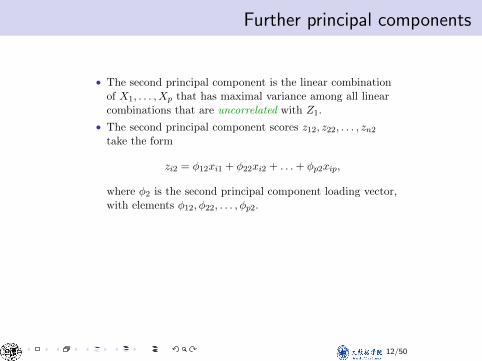
• The second principal component is the linear combinationof X1, . . . , Xp that has maximal variance among all linearcombinations that are uncorrelated with Z1.
• The second principal component scores z12, z22, . . . , zn2take the form
zi2 = φ12xi1 + φ22xi2 + . . .+ φp2xip,
where φ2 is the second principal component loading vector,with elements φ12, φ22, . . . , φp2.
11 / 52
12/50
Further principal componentsFurther principal components: continued
• It turns out that constraining Z2 to be uncorrelated withZ1 is equivalent to constraining the direction φ2 to beorthogonal (perpendicular) to the direction φ1. And so on.
• The principal component directions φ1, φ2, φ3, . . . are theordered sequence of right singular vectors of the matrix X,and the variances of the components are 1
n times thesquares of the singular values. There are at mostmin(n− 1, p) principal components.
12 / 52
12/50
ClusteringClustering
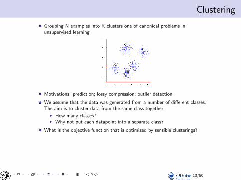
Grouping N examples into K clusters one of canonical problems inunsupervised learning
Motivations: prediction; lossy compression; outlier detection
We assume that the data was generated from a number of different classes.The aim is to cluster data from the same class together.
I How many classes?I Why not put each datapoint into a separate class?
What is the objective function that is optimized by sensible clusterings?
Urtasun & Zemel (UofT) CSC 411: 12-Clustering Oct 28, 2015 5 / 18
13/50
ClusteringClustering
• Clustering refers to a very broad set of techniques forfinding subgroups, or clusters, in a data set.
• We seek a partition of the data into distinct groups so thatthe observations within each group are quite similar toeach other,
• It make this concrete, we must define what it means fortwo or more observations to be similar or different.
• Indeed, this is often a domain-specific consideration thatmust be made based on knowledge of the data beingstudied.
23 / 52
13/50
ClusteringPCA vs Clustering
• PCA looks for a low-dimensional representation of theobservations that explains a good fraction of the variance.
• Clustering looks for homogeneous subgroups among theobservations.
24 / 52PCA vs Clustering
13/50
Two clustering methods
K-means clustering method: we seek to partition the observationsinto a pre-specied number of clusters. We introduceK-means and soft-Kmeans here.
hierarchical clustering method: we do not know in advance howmany clusters we want; in fact, we end up with atree-like visual representation of the observations,called a dendrogram, that allows us to view at oncethe clusterings obtained for each possible number ofclusters, from 1 to n.
14/50
The K-means clustering algorithmThe K-means algorithm
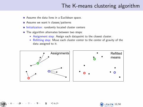
Assume the data lives in a Euclidean space.
Assume we want k classes/patterns
Initialization: randomly located cluster centers
The algorithm alternates between two steps:I Assignment step: Assign each datapoint to the closest cluster.I Refitting step: Move each cluster center to the center of gravity of the
data assigned to it.
Assignments Refitted means
Urtasun & Zemel (UofT) CSC 411: 12-Clustering Oct 28, 2015 6 / 18
15/50
K-means Objectives&DetailsK-means Objective
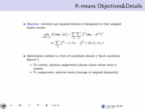
Objective: minimize sum squared distance of datapoints to their assignedcluster centers
min{m},{r}
E ({m}, {r}) =∑
n
∑
k
r(n)k ||mk − x(n)||2
s.t.∑
k
r(n)k = 1,∀n, r
(n)k ∈ {0, 1},∀k, n
Optimization method is a form of coordinate descent (”block coordinatedescent”)
I Fix centers, optimize assignments (choose cluster whose mean isclosest)
I Fix assignments, optimize means (average of assigned datapoints)
Urtasun & Zemel (UofT) CSC 411: 12-Clustering Oct 28, 2015 7 / 18
16/50
K-means Objectives&DetailsK-means
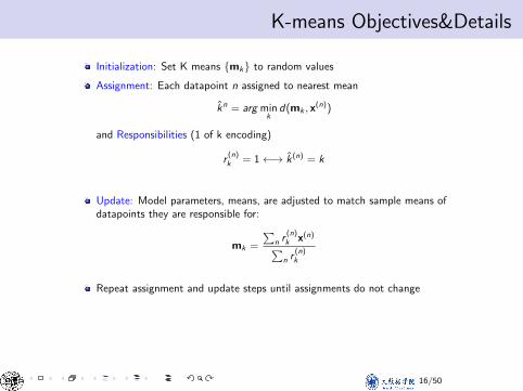
Initialization: Set K means {mk} to random values
Assignment: Each datapoint n assigned to nearest mean
k̂n = arg mink
d(mk , x(n))
and Responsibilities (1 of k encoding)
r(n)k = 1←→ k̂(n) = k
Update: Model parameters, means, are adjusted to match sample means ofdatapoints they are responsible for:
mk =
∑n r
(n)k x(n)
∑n r
(n)k
Repeat assignment and update steps until assignments do not change
Urtasun & Zemel (UofT) CSC 411: 12-Clustering Oct 28, 2015 8 / 18
16/50
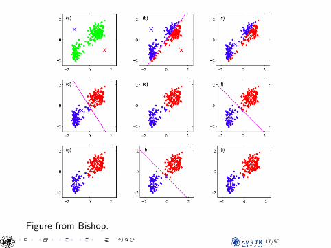
Figure from Bishop.
17/50
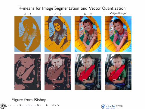
K-means for Image Segmentation and Vector Quantization:
Figure from Bishop.
17/50

Questions about K-meansQuestions about K-means
Why does update set mk to mean of assigned points?
Where does distance d come from?
What if we used a different distance measure?
How can we choose best distance?
How to choose K?
How can we choose between alternative clusterings?
Will it converge?
Hard cases – unequal spreads, non-circular spreads, inbetween points
Urtasun & Zemel (UofT) CSC 411: 12-Clustering Oct 28, 2015 12 / 18
18/50
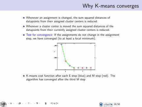
Why K-means convergesWhy K-means converges
Whenever an assignment is changed, the sum squared distances ofdatapoints from their assigned cluster centers is reduced.
Whenever a cluster center is moved the sum squared distances of thedatapoints from their currently assigned cluster centers is reduced.
Test for convergence: If the assignments do not change in the assignmentstep, we have converged (to at least a local minimum).
K-means cost function after each E step (blue) and M step (red). Thealgorithm has converged after the third M step
Urtasun & Zemel (UofT) CSC 411: 12-Clustering Oct 28, 2015 13 / 18
19/50
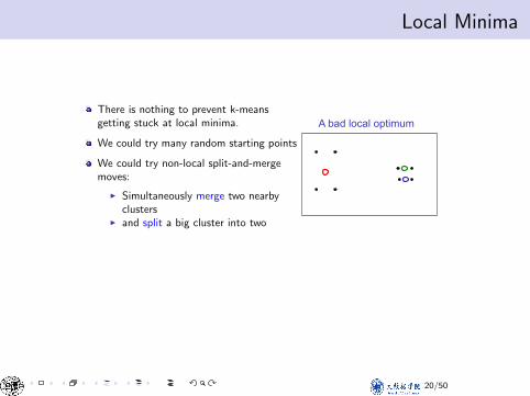
Local MinimaLocal Minima
There is nothing to prevent k-meansgetting stuck at local minima.
We could try many random starting points
We could try non-local split-and-mergemoves:
I Simultaneously merge two nearbyclusters
I and split a big cluster into two
A bad local optimum
Urtasun & Zemel (UofT) CSC 411: 12-Clustering Oct 28, 2015 14 / 18
20/50
Soft K-means AlgorithmSoft k-means
Instead of making hard assignments of datapoints to clusters, we can makesoft assignments. One cluster may have a responsibility of .7 for a datapointand another may have a responsibility of .3.
I Allows a cluster to use more information about the data in the refittingstep.
I What happens to our convergence guarantee?I How do we decide on the soft assignments?
Urtasun & Zemel (UofT) CSC 411: 12-Clustering Oct 28, 2015 15 / 18
21/50
Soft K-means AlgorithmSoft K-means Algorithm
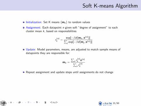
Initialization: Set K means {mk} to random values
Assignment: Each datapoint n given soft ”degree of assignment” to eachcluster mean k, based on responsibilities
r(n)k =
exp[−βd(mk , x(n))]∑j exp[−βd(mj , x(n))]
Update: Model parameters, means, are adjusted to match sample means ofdatapoints they are responsible for:
mk =
∑n r
(n)k x(n)
∑n r
(n)k
Repeat assignment and update steps until assignments do not change
Urtasun & Zemel (UofT) CSC 411: 12-Clustering Oct 28, 2015 16 / 18
21/50
Hierarchical ClusteringHierarchical Clustering
• K-means clustering requires us to pre-specify the numberof clusters K. This can be a disadvantage (later we discussstrategies for choosing K)
• Hierarchical clustering is an alternative approach whichdoes not require that we commit to a particular choice ofK.
• In this section, we describe bottom-up or agglomerativeclustering. This is the most common type of hierarchicalclustering, and refers to the fact that a dendrogram is builtstarting from the leaves and combining clusters up to thetrunk.
37 / 52
22/50
Visual Saliency Attention in a bottom-up way
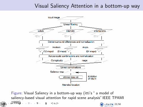
Figure: Visual Saliency in a bottom-up way (itti’s “ a model ofsaliency-based visual attention for rapid scene analysis” IEEE TPAMI1998) 23/50
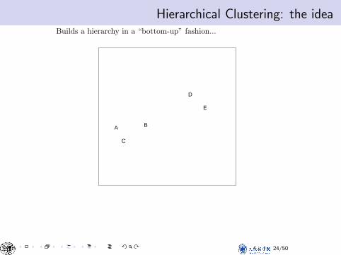
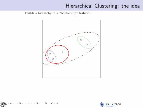
Hierarchical Clustering: the ideaHierarchical Clustering: the ideaBuilds a hierarchy in a “bottom-up” fashion...
A B
C
D
E
38 / 52
24/50
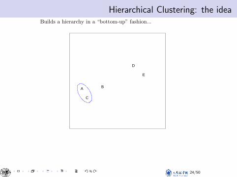
Hierarchical Clustering: the ideaHierarchical Clustering: the ideaBuilds a hierarchy in a “bottom-up” fashion...
A B
C
D
E
38 / 52
24/50
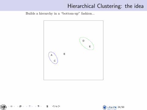
Hierarchical Clustering: the ideaHierarchical Clustering: the ideaBuilds a hierarchy in a “bottom-up” fashion...
A B
C
D
E
38 / 52
24/50
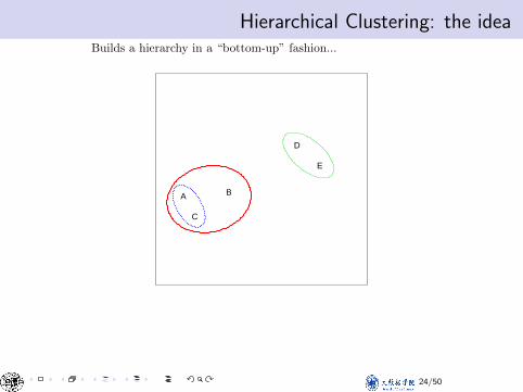
Hierarchical Clustering: the ideaHierarchical Clustering: the ideaBuilds a hierarchy in a “bottom-up” fashion...
A B
C
D
E
38 / 52
24/50
Hierarchical Clustering: the ideaHierarchical Clustering: the ideaBuilds a hierarchy in a “bottom-up” fashion...
A B
C
D
E
38 / 52
24/50
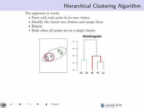
Hierarchical Clustering AlgorithmHierarchical Clustering AlgorithmThe approach in words:
• Start with each point in its own cluster.• Identify the closest two clusters and merge them.• Repeat.• Ends when all points are in a single cluster.
A BC
DE
01
23
4
Dendrogram
D E B A C
39 / 52
25/50
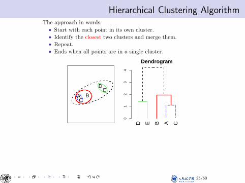
Hierarchical Clustering AlgorithmHierarchical Clustering AlgorithmThe approach in words:
• Start with each point in its own cluster.• Identify the closest two clusters and merge them.• Repeat.• Ends when all points are in a single cluster.
A BC
DE
01
23
4
Dendrogram
D E B A C
39 / 52
25/50
An Example of Hierarchical ClusteringAn Example
−6 −4 −2 0 2−
20
24
X1
X2
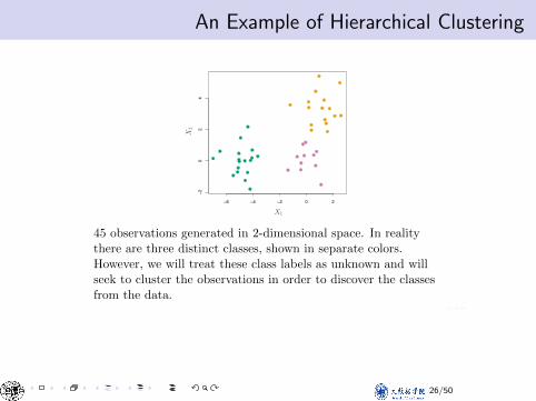
45 observations generated in 2-dimensional space. In realitythere are three distinct classes, shown in separate colors.However, we will treat these class labels as unknown and willseek to cluster the observations in order to discover the classesfrom the data.
40 / 52
26/50

An Example of Hierarchical ClusteringApplication of hierarchical clustering
02
46
81
0
02
46
81
0
02
46
81
0
41 / 52
26/50
An Example of Hierarchical ClusteringDetails of previous figure
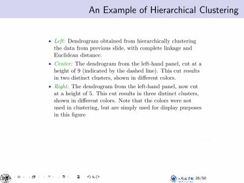
• Left: Dendrogram obtained from hierarchically clusteringthe data from previous slide, with complete linkage andEuclidean distance.
• Center: The dendrogram from the left-hand panel, cut at aheight of 9 (indicated by the dashed line). This cut resultsin two distinct clusters, shown in different colors.
• Right: The dendrogram from the left-hand panel, now cutat a height of 5. This cut results in three distinct clusters,shown in different colors. Note that the colors were notused in clustering, but are simply used for display purposesin this figure
42 / 52
26/50
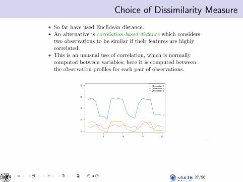
Choice of Dissimilarity MeasureChoice of Dissimilarity Measure
• So far have used Euclidean distance.• An alternative is correlation-based distance which considers
two observations to be similar if their features are highlycorrelated.
• This is an unusual use of correlation, which is normallycomputed between variables; here it is computed betweenthe observation profiles for each pair of observations.
5 10 15 20
05
10
15
20
Variable Index
Observation 1
Observation 2
Observation 3
1
2
3
46 / 52
27/50

ConclusionConclusions
• Unsupervised learning is important for understanding thevariation and grouping structure of a set of unlabeled data,and can be a useful pre-processor for supervised learning
• It is intrinsically more difficult than supervised learningbecause there is no gold standard (like an outcomevariable) and no single objective (like test set accuracy)
• It is an active field of research, with many recentlydeveloped tools such as self-organizing maps, independentcomponents analysis and spectral clustering.See The Elements of Statistical Learning, chapter 14.
52 / 52
28/50

Gaussian Mixture Model (GMM)
29/50
A generative view of clusteringA generative view of clustering
Last time: hard and soft k-means algorithm
Today: statistical formulation of clustering → principled, justification forupdates
We need a sensible measure of what it means to cluster the data well.
I This makes it possible to judge different methods.I It may help us decide on the number of clusters.
An obvious approach is to imagine that the data was produced by agenerative model.
I Then we adjust the model parameters to maximize the probability thatit would produce exactly the data we observed.
Urtasun & Zemel (UofT) CSC 411: 13-MoG Nov 2, 2015 3 / 31
30/50
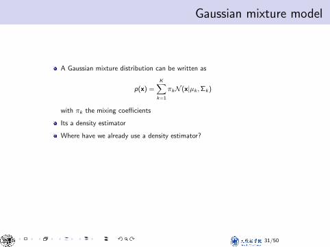
Gaussian mixture modelGaussian mixture model
A Gaussian mixture distribution can be written as
p(x) =K∑
k=1
πkN (x|µk ,Σk)
with πk the mixing coefficients
Urtasun & Zemel (UofT) CSC 411: 13-MoG Nov 2, 2015 4 / 31
31/50
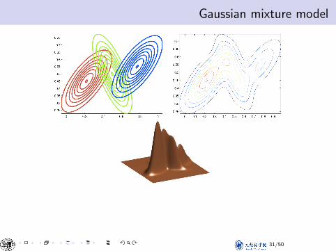
Gaussian mixture modelVisualizing a Mixture of Gaussians
Urtasun & Zemel (UofT) CSC 411: 13-MoG Nov 2, 2015 5 / 31
31/50
Gaussian mixture modelGaussian mixture model
A Gaussian mixture distribution can be written as
p(x) =K∑
k=1
πkN (x|µk ,Σk)
with πk the mixing coefficients
Its a density estimator
Where have we already use a density estimator?
Urtasun & Zemel (UofT) CSC 411: 13-MoG Nov 2, 2015 6 / 31
31/50
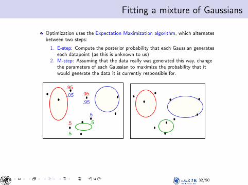
Fitting a mixture of GaussiansFitting a mixture of Gaussians
Optimization uses the Expectation Maximization algorithm, which alternatesbetween two steps:
1. E-step: Compute the posterior probability that each Gaussian generateseach datapoint (as this is unknown to us)
2. M-step: Assuming that the data really was generated this way, changethe parameters of each Gaussian to maximize the probability that itwould generate the data it is currently responsible for.
.95
.5
.5
.05
.5 .5
.95 .05
Urtasun & Zemel (UofT) CSC 411: 13-MoG Nov 2, 2015 7 / 31
32/50
Latent Variable ModelsLatent Variable Models
Some model variables may be unobserved, either at training or at test time,or both
If occasionally unobserved they are missing, e.g., undefined inputs, missingclass labels, erroneous targets
Variables which are always unobserved are called latent variables, orsometimes hidden variables
We may want to intentionally introduce latent variables to model complexdependencies between variables – this can actually simplify the model
Form of divide-and-conquer: use simple parts to build complex models
In a mixture model, the identity of the component that generated a givendatapoint is a latent variable
Urtasun & Zemel (UofT) CSC 411: 13-MoG Nov 2, 2015 8 / 31
33/50
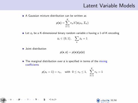
Latent Variable ModelsLatent variables in mixture models
A Gaussian mixture distribution can be written as
p(x) =K∑
k=1
πkN (x|µk ,Σk)
Let zk be a K-dimensional binary random variable z having a 1-of-K encoding
zk ∈ {0, 1},∑
k
zk = 1
Joint distributionp(x, z) = p(x|z)p(z)
The marginal distribution over z is specified in terms of the mixingcoefficients
p(zk = 1) = πk , with 0 ≤ πk ≤ 1,K∑
k=1
πk = 1
Urtasun & Zemel (UofT) CSC 411: 13-MoG Nov 2, 2015 9 / 31
33/50
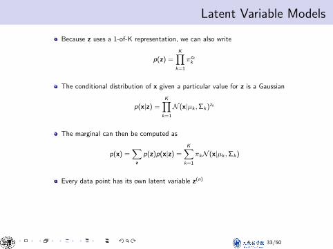
Latent Variable ModelsLatent variables in mixture models
Because z uses a 1-of-K representation, we can also write
p(z) =K∏
k=1
πzkk
The conditional distribution of x given a particular value for z is a Gaussian
p(x|z) =K∏
k=1
N (x|µk ,Σk)zk
The marginal can then be computed as
p(x) =∑
z
p(z)p(x|z) =K∑
k=1
πkN (x|µk ,Σk)
Every data point has its own latent variable z(n)
Urtasun & Zemel (UofT) CSC 411: 13-MoG Nov 2, 2015 10 / 31
33/50
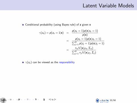
Latent Variable ModelsResponsabilities
Conditional probability (using Bayes rule) of z given x
γ(zk) = p(zk = 1|x) =p(zk = 1)p(x|zk = 1)
p(x)
=p(zk = 1)p(x|zk = 1)
∑Kj=1 p(zj = 1)p(x|zj = 1)
=πkN (x|µk ,Σk)
∑Kj=1 πjN (x|µj ,Σj)
γ(zk) can be viewed as the responsibility
Urtasun & Zemel (UofT) CSC 411: 13-MoG Nov 2, 2015 11 / 31
33/50
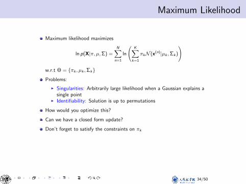
Maximum LikelihoodMaximum Likelihood
Maximum likelihood maximizes
ln p(X|π, µ,Σ) =N∑
n=1
ln
(K∑
k=1
πkN (x(n)|µk ,Σk)
)
w.r.t Θ = {πk , µk ,Σk}Problems:
I Singularities: Arbitrarily large likelihood when a Gaussian explains asingle point
I Identifiability: Solution is up to permutations
How would you optimize this?
Can we have a closed form update?
Don’t forget to satisfy the constraints on πk
Urtasun & Zemel (UofT) CSC 411: 13-MoG Nov 2, 2015 13 / 31
34/50

Objective: Expected Complete Data LikelihoodObjective: Expected Complete Data Likelihood
Maximum likelihood maximizes
ln p(X|π, µ,Σ) =N∑
n=1
ln
(K∑
k=1
πkN (x(n)|µk ,Σk)
)
Hard to maximize (log-)likelihood of data directly
General problem: sum inside the log
ln p(x|Θ) = ln∑
z
p(x, z|Θ)
Urtasun & Zemel (UofT) CSC 411: 13-MoG Nov 2, 2015 14 / 31
35/50
Expectation MaximizationExpectation Maximization
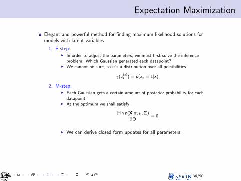
Elegant and powerful method for finding maximum likelihood solutions formodels with latent variables
1. E-step:I In order to adjust the parameters, we must first solve the inference
problem: Which Gaussian generated each datapoint?I We cannot be sure, so it’s a distribution over all possibilities.
γ(z(n)k ) = p(zk = 1|x)
2. M-step:I Each Gaussian gets a certain amount of posterior probability for each
datapoint.I At the optimum we shall satisfy
∂ ln p(X|π, µ,Σ)
∂Θ= 0
I We can derive closed form updates for all parameters
Urtasun & Zemel (UofT) CSC 411: 13-MoG Nov 2, 2015 15 / 31
36/50
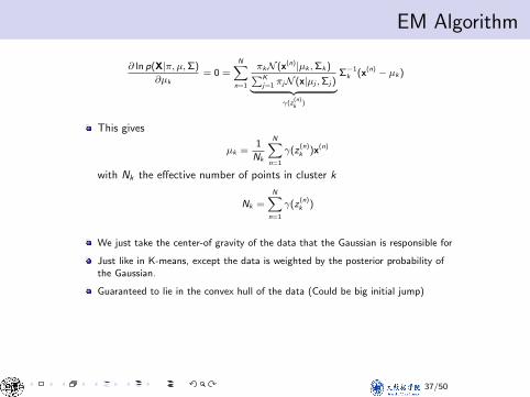
EM AlgorithmM-Step (mean)
∂ ln p(X|π, µ,Σ)
∂µk= 0 =
N∑
n=1
πkN (x(n)|µk ,Σk)∑Kj=1 πjN (x|µj ,Σj)︸ ︷︷ ︸
γ(z(n)k
)
Σ−1k (x(n) − µk)
This gives
µk =1
Nk
N∑
n=1
γ(z(n)k )x(n)
with Nk the effective number of points in cluster k
Nk =N∑
n=1
γ(z(n)k )
We just take the center-of gravity of the data that the Gaussian is responsible for
Just like in K-means, except the data is weighted by the posterior probability ofthe Gaussian.
Guaranteed to lie in the convex hull of the data (Could be big initial jump)
Urtasun & Zemel (UofT) CSC 411: 13-MoG Nov 2, 2015 16 / 31
37/50
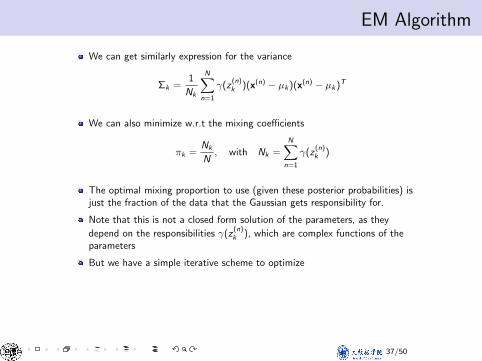
EM AlgorithmM-Step (variance, mixing coefficients)
We can get similarly expression for the variance
Σk =1
Nk
N∑
n=1
γ(z(n)k )(x(n) − µk)(x(n) − µk)T
We can also minimize w.r.t the mixing coefficients
πk =Nk
N, with Nk =
N∑
n=1
γ(z(n)k )
The optimal mixing proportion to use (given these posterior probabilities) isjust the fraction of the data that the Gaussian gets responsibility for.
Note that this is not a closed form solution of the parameters, as they
depend on the responsibilities γ(z(n)k ), which are complex functions of the
parameters
But we have a simple iterative scheme to optimize
Urtasun & Zemel (UofT) CSC 411: 13-MoG Nov 2, 2015 17 / 31
37/50
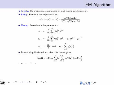
EM AlgorithmEM Algorithm
Initialize the means µk , covariances Σk and mixing coefficients πk
E-step: Evaluate the responsibilities
γ(zk) = p(zk = 1|x) =πkN (x|µk ,Σk)∑Kj=1 πjN (x|µj ,Σj)
M-step: Re-estimate the parameters
µk =1
Nk
N∑
n=1
γ(z(n)k )x(n)
Σk =1
Nk
N∑
n=1
γ(z(n)k )(x(n) − µk)(x(n) − µk)T
πk =Nk
Nwith Nk =
N∑
n=1
γ(z(n)k )
Evaluate log likelihood and check for convergence
ln p(X|π, µ,Σ) =N∑
n=1
ln
(K∑
k=1
πkN (x(n)|µk ,Σk)
)
Continue loopingUrtasun & Zemel (UofT) CSC 411: 13-MoG Nov 2, 2015 18 / 31
37/50
An Alternative View of EMAn Alternative View of EM
Hard to maximize (log-)likelihood of data directly
General problem: sum inside the log
ln p(x|Θ) = ln∑
z
p(x, z|Θ)
Complete data {x, z}, and x is the incomplete data
If we knew z , then easy to maximize (replace sum over k with just the kwhere zk = 1)
Unfortunately we are not given the complete data, but only the incomplete.
Our knowledge about the latent variables is p(Z|X,Θold)
In the E-step we compute p(Z|X,Θold)
In the M-step we maximize w.r.t Θ
Q(Θ,Θold) =∑
z
p(Z|X,Θold) ln p(X,Z|Θ)
Urtasun & Zemel (UofT) CSC 411: 13-MoG Nov 2, 2015 20 / 31
38/50
General EM AlgorithmGeneral EM Algorithm
1. Initialize Θold
2. E-step: Evaluate p(Z|X,Θold)
3. M-step:Θnew = arg max
ΘQ(Θ,Θold)
whereQ(Θ,Θold) =
∑
z
p(Z|X,Θold) ln p(X,Z|Θ)
4. Evaluate log likelihood and check for convergence (or the parameters). Ifnot converged, Θold = Θ, Go to step 2
Urtasun & Zemel (UofT) CSC 411: 13-MoG Nov 2, 2015 21 / 31
39/50

How do we know that the updates improve things?How do we know that the updates improve things?
Updating each Gaussian definitely improves the probability of generating thedata if we generate it from the same Gaussians after the parameter updates.
I But we know that the posterior will change after updating theparameters.
A good way to show that this is OK is to show that there is a single functionthat is improved by both the E-step and the M-step.
I The function we need is called Free Energy.
Urtasun & Zemel (UofT) CSC 411: 13-MoG Nov 2, 2015 22 / 31
40/50

Why EM convergesWhy EM converges
Free energy F is a cost function that is reduced by both the E-step and theM-step.
F = expected energy− entropy
The expected energy term measures how difficult it is to generate eachdatapoint from the Gaussians it is assigned to. It would be happiestassigning each datapoint to the Gaussian that generates it most easily (as inK-means).
The entropy term encourages ”soft” assignments. It would be happiestspreading the assignment probabilities for each datapoint equally between allthe Gaussians.
Urtasun & Zemel (UofT) CSC 411: 13-MoG Nov 2, 2015 23 / 31
41/50
Free EnergyFree Energy
Our goal is to maximize
p(X|Θ) =∑
z
p(X, z|Θ)
Typically optimizing p(X|Θ) is difficult, but p(X,Z|Θ) is easy
Let q(Z) be a distribution over the latent variables. For any distributionq(Z) we have
ln p(X|Θ) = L(q,Θ) + KL(q||p(Z|X,Θ))
where
L(q,Θ) =∑
Z
q(Z) ln
{p(X,Z|Θ)
q(Z)
}
KL(q||p) = −∑
Z
q(Z) ln
{p(Z|X,Θ)
q(Z)
}
Urtasun & Zemel (UofT) CSC 411: 13-MoG Nov 2, 2015 24 / 31
42/50

More on Free EnergyMore on Free Energy
Since the KL-divergence is always positive and have value 0 only ifq(Z ) = p(Z|X,Θ)
Thus L(q,Θ) is a lower bound on the likelihood
L(q,Θ) ≤ ln p(X|Θ)
Urtasun & Zemel (UofT) CSC 411: 13-MoG Nov 2, 2015 25 / 31
43/50
E-step and M-stepE-step and M-step
ln p(X|Θ) = L(q,Θ) + KL(q||p(Z|X,Θ))
In the E-step we maximize w.r.t q(Z) the lower bound L(q,Θ)
Since ln p(X|θ) does not depend on q(Z), the maximum L is obtained whenthe KL is 0
This is achieved when q(Z) = p(Z|X,Θ)
The lower bound L is then
L(q,Θ) =∑
Z
p(Z|X,Θold) ln p(X,Z|Θ)−∑
Z
p(Z|X,Θold) ln p(Z|X,Θold)
= Q(Θ,Θold) + const
with the content the entropy of the q distribution, which is independent of Θ
In the M-step the quantity to be maximized is the expectation of thecomplete data log-likelihood
Note that Θ is only inside the logarithm and optimizing the complete datalikelihood is easier
Urtasun & Zemel (UofT) CSC 411: 13-MoG Nov 2, 2015 26 / 31
44/50
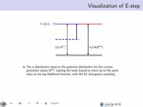
Visualization of E-stepVisualization of E-step
The q distribution equal to the posterior distribution for the currentparameter values Θold , causing the lower bound to move up to the samevalue as the log likelihood function, with the KL divergence vanishing.
Urtasun & Zemel (UofT) CSC 411: 13-MoG Nov 2, 2015 27 / 31
45/50
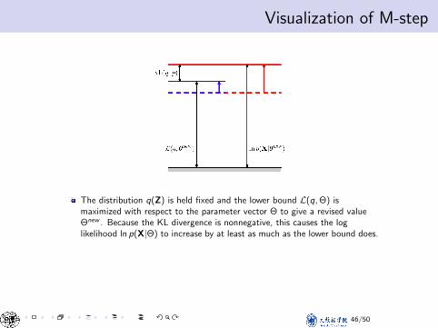
Visualization of M-stepVisualization of M-step
The distribution q(Z) is held fixed and the lower bound L(q,Θ) ismaximized with respect to the parameter vector Θ to give a revised valueΘnew . Because the KL divergence is nonnegative, this causes the loglikelihood ln p(X|Θ) to increase by at least as much as the lower bound does.
Urtasun & Zemel (UofT) CSC 411: 13-MoG Nov 2, 2015 28 / 31
46/50
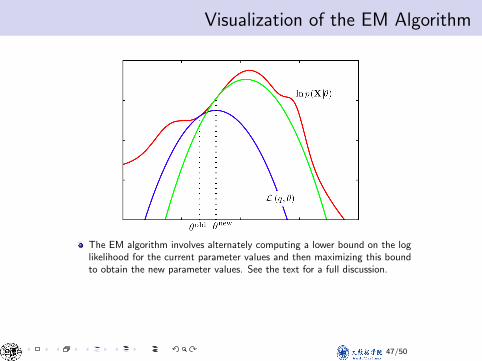
Visualization of the EM AlgorithmVisualization of the EM Algorithm
The EM algorithm involves alternately computing a lower bound on the loglikelihood for the current parameter values and then maximizing this boundto obtain the new parameter values. See the text for a full discussion.
Urtasun & Zemel (UofT) CSC 411: 13-MoG Nov 2, 2015 29 / 31
47/50
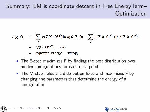
Summary: EM is coordinate descent in Free EnergyTerm–Optimization
• The E-step maximizes F by finding the best distribution overhidden configurations for each data point.
• The M-step holds the distribution fixed and maximizes F bychanging the parameters that determine the energy of aconfiguration.
48/50
Mixture of Gaussians vs. K-meansMixture of Gaussians vs. K-means
EM for mixtures of Gaussians is just like a soft version of K-means, withfixed priors and covariance
Instead of hard assignments in the E-step, we do soft assignments based onthe softmax of the squared Mahalanobis distance from each point to eachcluster.
Each center moved by weighted means of the data, with weights given bysoft assignments
In K-means, weights are 0 or 1
Urtasun & Zemel (UofT) CSC 411: 13-MoG Nov 2, 2015 31 / 31
49/50
Acknowledgement
Acknowledgement
Some slides are in courtesy of(1)Chap 10 of James et. al. “An Introduction to StatisticalLearning with applications in R”, 2011;(2) Lecture 12,13, Raquel Urtasun & Rich Zemel, University ofToronto.
50/50