Introduction to Stata fileStata: Only one dataset open at once (but we can combine several fles....
148
1 / 148 Introduction to Stata UiO, November 1st 2018, Knut Waagan
Transcript of Introduction to Stata fileStata: Only one dataset open at once (but we can combine several fles....

1 / 148
Introduction to Stata
UiO, November 1st 2018, Knut Waagan

2 / 148
Goals
Getting started Data management techniques Get an overview

3 / 148
Topics
Handling data sets Descriptive statistics Make graphs Some estimation
4 / 148
Part 1: A frst example
Typing in data Setting variable names Creating a diagram Storing data Get familiar

5 / 148
The main window
5 subwindows Drop-down
menus
6 / 148
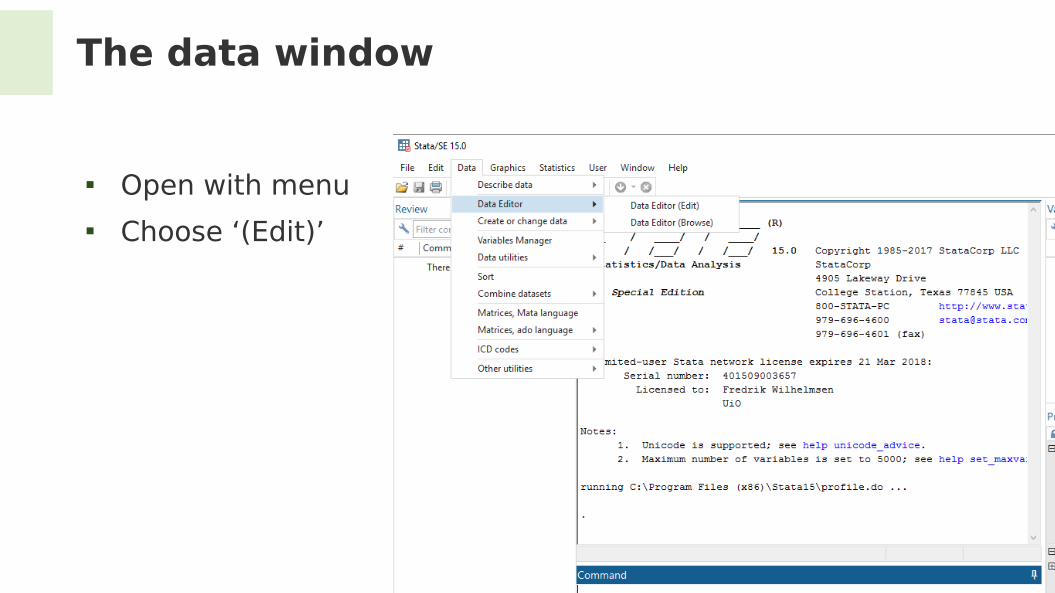
The data window
Open with menu Choose ‘(Edit)’
7 / 148
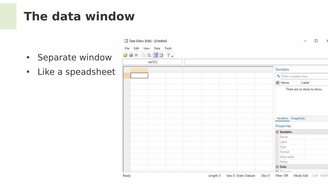
The data window
Separate window Like a speadsheet
8 / 148
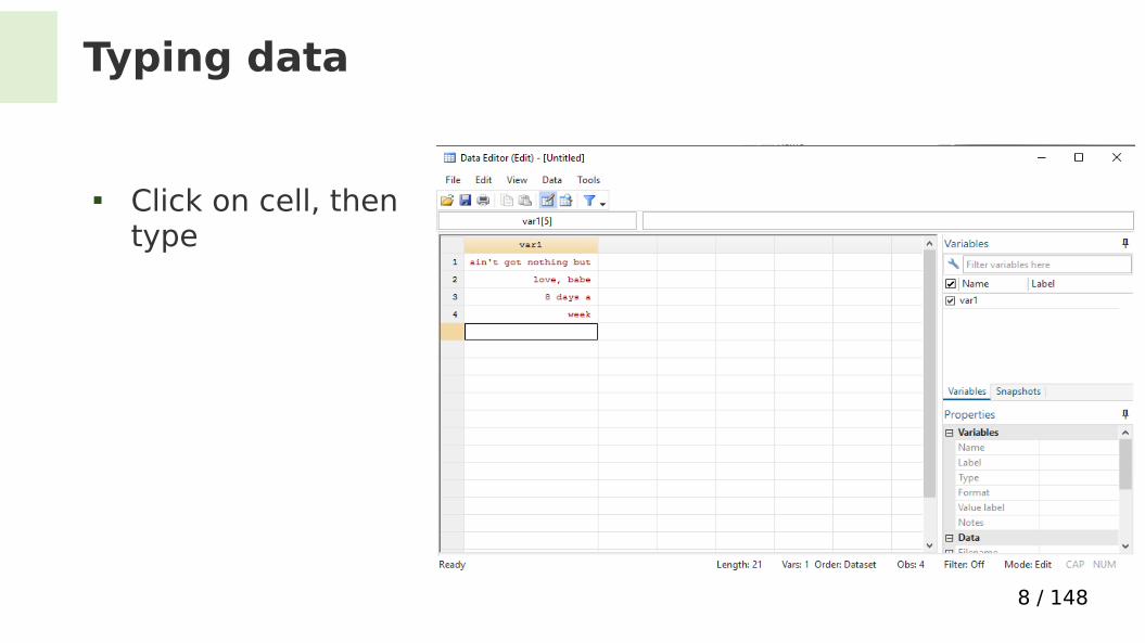
Typing data
Click on cell, then type

9 / 148
Typing data
Numbers or text Text values in red

10 / 148
Variable names
Name of columns Called variables Can be entered
here Case sensitive Whitespace not
allowed Customary to use
lower case

11 / 148
Browse mode – Look, don’t touch
Disable editing by selecting magnifying glass instead of pencil

12 / 148
A pie chart
In main menu Let’s graph the
chord abundance

13 / 148
A pie chart
Choose variable

14 / 148
A pie chart
Title, caption Click ‘Submit’

15 / 148
A pie chart
In separate window:

16 / 148
Why ‘Submit’?
‘OK’ = make plot & close window
‘Submit’ = make plot
Useful for trial and error etc
17 / 148
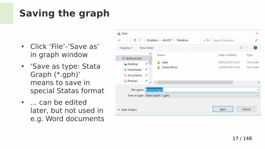
Saving the graph
Click ‘File’-’Save as’ in graph window
‘Save as type: Stata Graph (*.gph)’ means to save in special Statas format
... can be edited later, but not used in e.g. Word documents

18 / 148
Saving the graph
For including in reports etc, store as e.g. a png-image

19 / 148
Saving the data set
File - Save

20 / 148
Saving the data set
File - Save Special Stata
format (fle ending .dta)
21 / 148
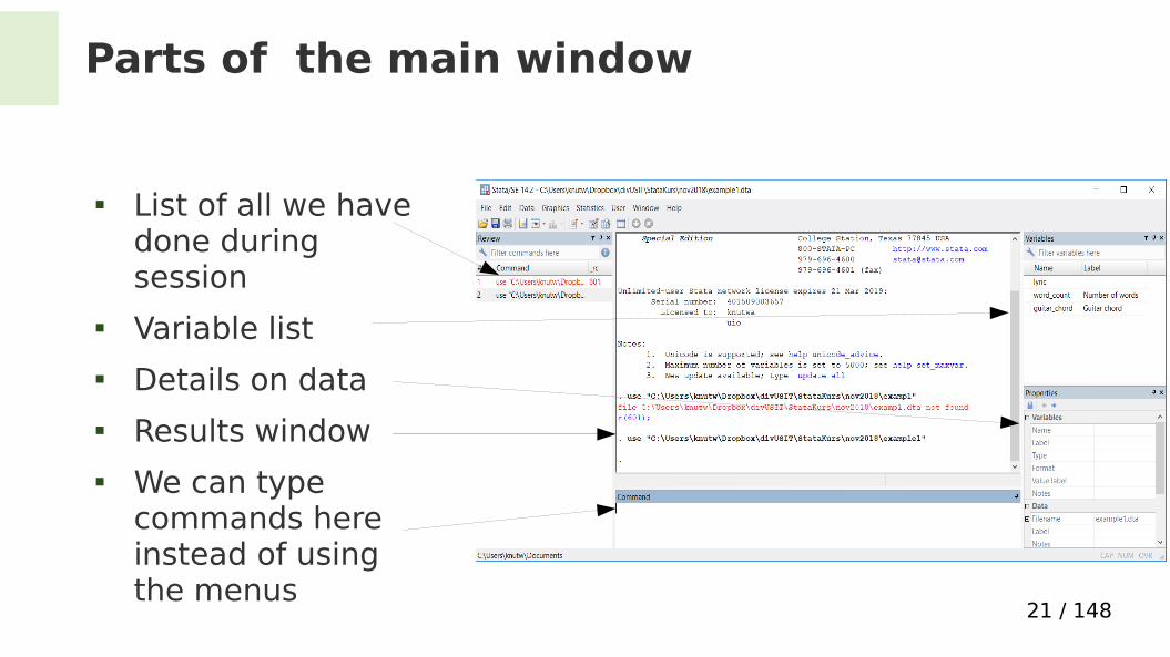
Parts of the main window
List of all we have done during session
Variable list Details on data Results window We can type
commands here instead of using the menus
22 / 148
Part 2: Data management 1
Loading from a fle Dataset structure: observations/variables, values,
strings/numbers Value labels list, selecting observations with if and in
23 / 148
A prepared dataset
We start with a dataset that’s already prepared:
http://www.stata-press.com/data/r14/states.dta We look at its structure ... and how to select subsets of it

24 / 148
Loading data
For data fles in the Stata-format .dta
Use ‘Import’ to load from other formats
25 / 148
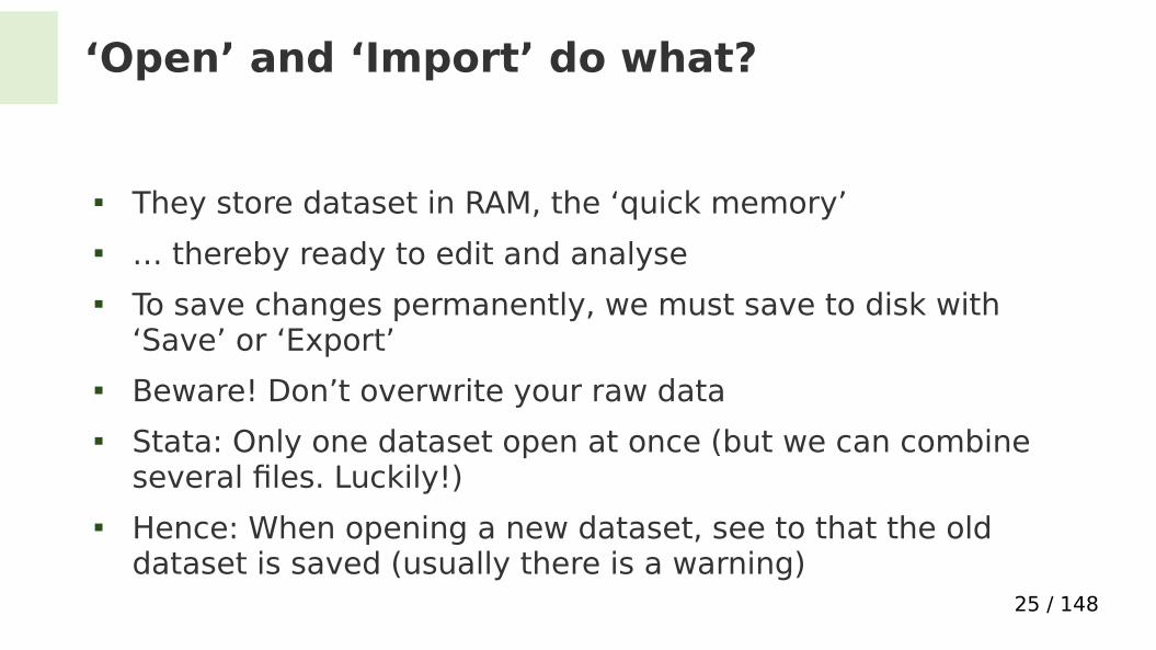
‘Open’ and ‘Import’ do what?
They store dataset in RAM, the ‘quick memory’ … thereby ready to edit and analyse To save changes permanently, we must save to disk with
‘Save’ or ‘Export’ Beware! Don’t overwrite your raw data Stata: Only one dataset open at once (but we can combine
several fles. Luckily!) Hence: When opening a new dataset, see to that the old
dataset is saved (usually there is a warning)

26 / 148
Dataset structure
Columns: Variables Row: Obervations, aka
data points Each cells contains a
value Variables have names and
labels

27 / 148
Data types
Red: Text (referred to as a string)
No colour: Numeric values Blue: Categorical variable Variables (i.e. columns)
have a fxed type
28 / 148
Variable types
Continuous variables: Age, temperature, income, number of citizens...
Categorical variables: Region, gender, type of drug… Ordered categorical/ordinal: Education level, grades...

29 / 148
Categorical variables in Stata
Stata prefers numbers in the cells
Text often best for the user
‘Value labels’: We can have both

30 / 148
Value labels: where in Stata?
Choose ‘Manage value labels’
Or click here

31 / 148
Value labels
Click the +
32 / 148
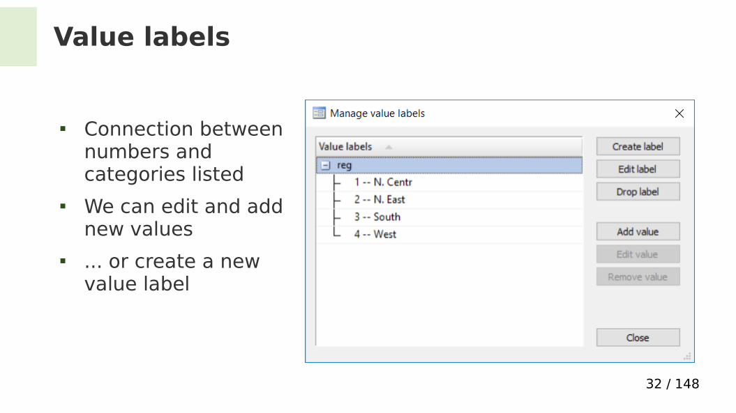
Value labels
Connection between numbers and categories listed
We can edit and add new values
... or create a new value label

33 / 148
Codebook
For a quick look at the labels:

34 / 148
Codebook
Choose variable Possibly more than one

35 / 148
Codebook, the result Could have just typed command

36 / 148
Ordered categorical, aka ordinal
Like categorical, but:

37 / 148
Ordered categorical, aka ordinal
Like categorical, but ... the order must be right

38 / 148
Reusing a value label
Time saving tip: The same value label can
be used for many variables
Put the name of the value label here

39 / 148
Listing – a typical Stata-command
List data in the results window

40 / 148
Listing
List data in the results window
Choose rows
41 / 148
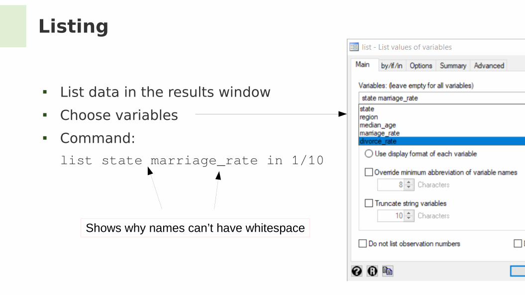
Listing
List data in the results window Choose variables Command:
list state marriage_rate in 1/10
Shows why names can’t have whitespace

42 / 148
Listing
The result:

43 / 148
Selection with if
Pick all data with median age above 32:
Command:
list if median_age > 32

44 / 148
Selection with if
Other examples:
list if state==”KANSAS”
list if state!=”KANSAS”
list if state!=”KANSAS” in 1/10
list if marriage_rate>100 & median_age<28
list if marriage_rate>100 | median_age<28
The statements after if are called ‘logical expressions’ Text-value in quotation marks, e.g. ”KANSAS”
‘equals’
‘and’/’or’
‘does not equal’

45 / 148
Selection with value labels
Two ways:
list if region==4
list if region==”West”:reg

46 / 148
Del 3: Data management 2
Importing data Creating categories with encode Create new variables Missing values Documenting work Combining data sets
47 / 148
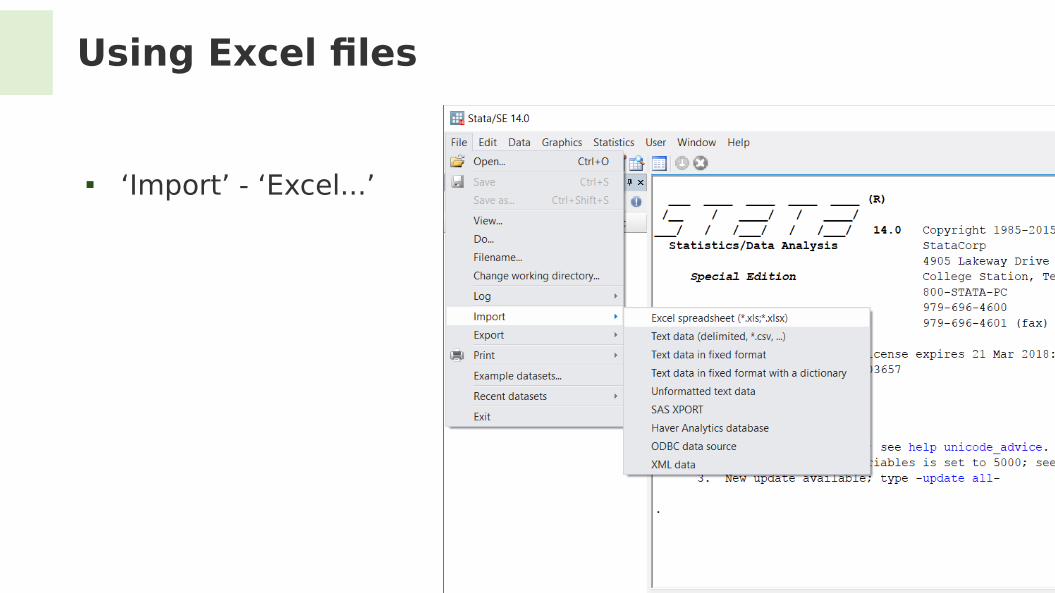
Using Excel fles
‘Import’ - ‘Excel...’

48 / 148
Using Excel fles
Create variable names from 1st row
Preview

49 / 148
Using Excel fles
What’s diferent?
50 / 148
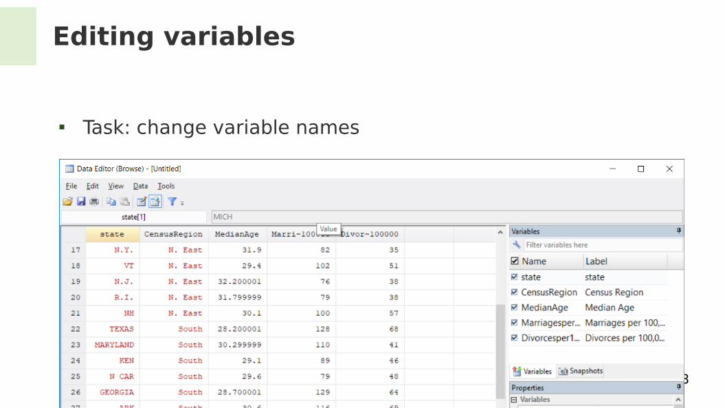
Editing variables
Task: change variable names

51 / 148
Number format
Change to 5 characters

52 / 148
Number format

53 / 148
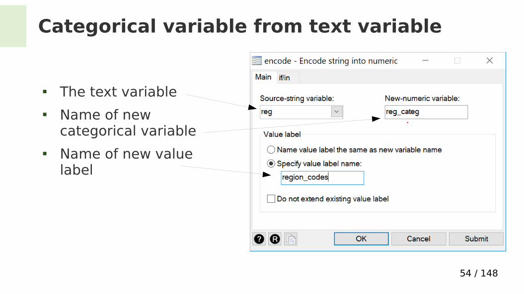
Categorical variable from text variable
Command: encode region, generate(region_num)
54 / 148
Categorical variable from text variable
The text variable Name of new
categorical variable Name of new value
label
55 / 148
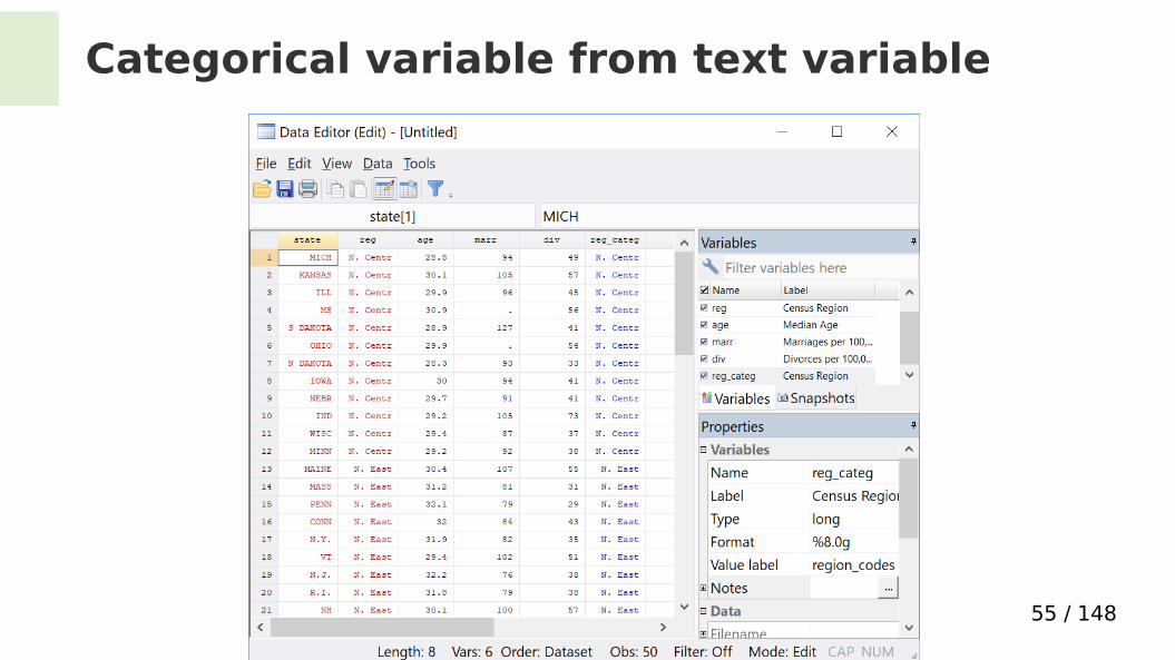
Categorical variable from text variable

56 / 148
Documentation
Store commands in a fle as text And: Stata can execute them at the push of a button! Called a Do-fle: Filendelse .do Open Do-fle-window here
57 / 148
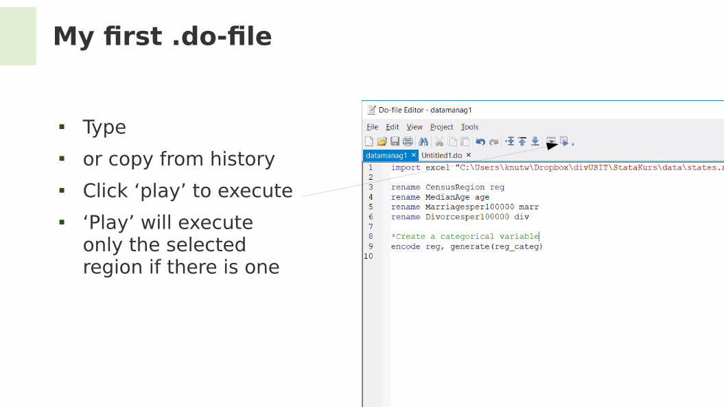
My frst .do-fle
Type or copy from history Click ‘play’ to execute ‘Play’ will execute
only the selected region if there is one

58 / 148
My frst .do-fle
Type or copy from history Click ‘play’ to execute ‘Play’ will execute
only the selected region if there is one
To save do-fle: Click ‘File’-’Save’

59 / 148
My frst .do-fle
Saving The fle is called a do-fle, syntax-fle or
(Stata-)script

60 / 148
My frst .do-fle
A comment The * tells Stata ‘this line is not a
command’

61 / 148
do-fles, why?
Documentation: for self and others Debugging: easier to pinpoint where it goes wrong Flexibility: Easy to make changes Recycling: e.g. if new data & same analysis ‘But I like the menus’? ... No problem, just paste the command into the do-fle
afterwards

62 / 148
Creating new variables
We can use a dialogue box:
63 / 148
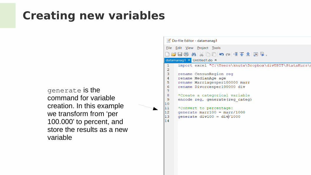
Creating new variables
generate is the command for variable creation. In this example we transform from ‘per 100.000’ to percent, and store the results as a new variable
64 / 148
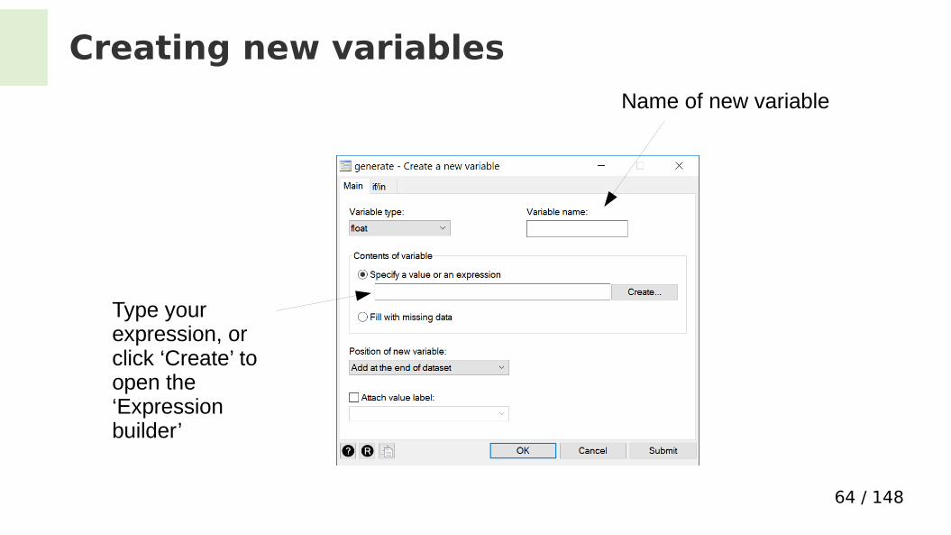
Creating new variables
Name of new variable
Type your expression, or click ‘Create’ to open the ‘Expression builder’

65 / 148
Creating new variables
Choose variables from list, choose e.g. ‘division’ from calculator

66 / 148
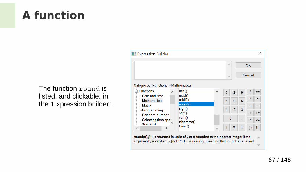
A function
The function round rounds off to nearest integer
Example:If the input is 28.2the output is 28
67 / 148
A function
The function round is listed, and clickable, in the ‘Expression builder’.

68 / 148
Saving results
Tables etc. show up in the results window
How to save them permanently?
69 / 148
Saving results: log
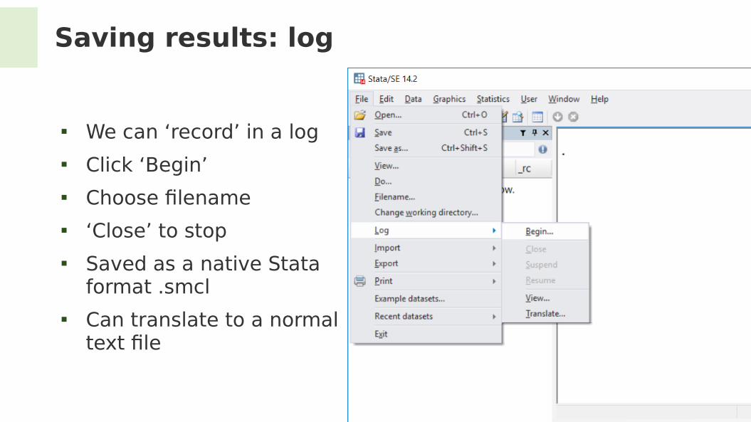
We can ‘record’ in a log Click ‘Begin’ Choose flename ‘Close’ to stop Saved as a native Stata
format .smcl Can translate to a normal
text fle
70 / 148
Copy-paste
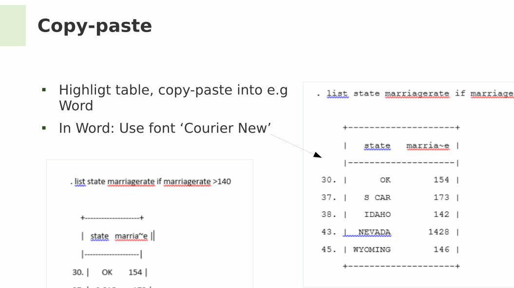
Highligt table, copy-paste into e.g Word
In Word: Use font ‘Courier New’

71 / 148
More advanced copy-paste
Highlight and right-click
table (for Excel, tsv)
html-table screenshot
72 / 148
Missing values
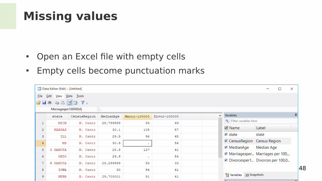
Open an Excel fle with empty cells Empty cells become punctuation marks

73 / 148
Missing values
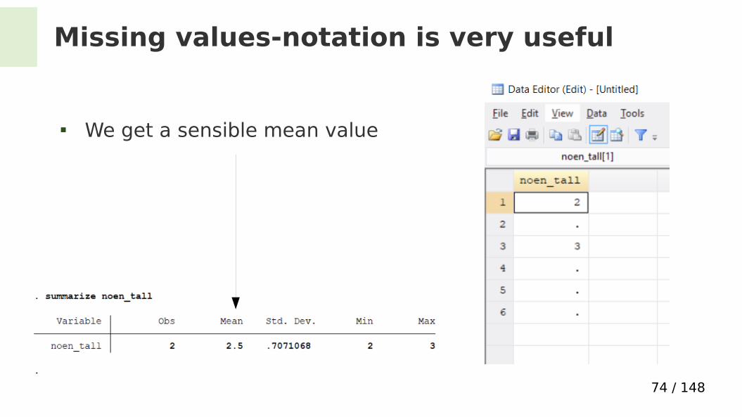
Punctuation mark means ‘missing value’ Stata commands understand this notation
74 / 148
Missing values-notation is very useful
We get a sensible mean value

75 / 148
But beware!
The value . is treated as a very large number (larger than any other)

76 / 148
But beware!
Solution:
list if Marr>200 & Marr<.
Also note abbreviated variable name Marriagesper100000

77 / 148
Opening a csv-fle
‘Import’-‘Text data (delimited, *.csv, ...)’ Comma-separated values Example

78 / 148
Combining data sets
What if data sit in separate fles?
New obses
Add observations: append Add variables: merge
New varsNew obses

79 / 148
Combining data sets
Stata: only one dataset at a time New data must be read from Stata fle (*.dta) ... so may need to convert fle to .dta frst
Add observations: append Add variables: merge
New varsNew obsesNew obses

80 / 148
Combining data sets
append matches variable names merge matches values of ‘key’ variable, e.g. a person’s ID-
number
Add observations: append Add variables: merge
New varsNew obses

81 / 148
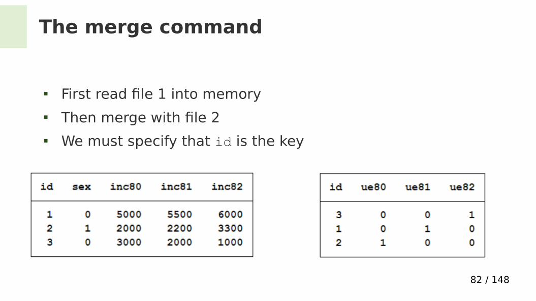
The merge command
Task: combine these two data fles Which rows belong together?
82 / 148
The merge command
First read fle 1 into memory Then merge with fle 2 We must specify that id is the key
83 / 148
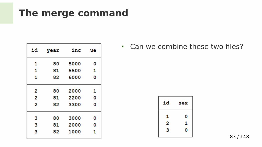
The merge command
Can we combine these two fles?

84 / 148
The merge command
Can we combine these two fles? Yes, with a many-to-one merge
85 / 148
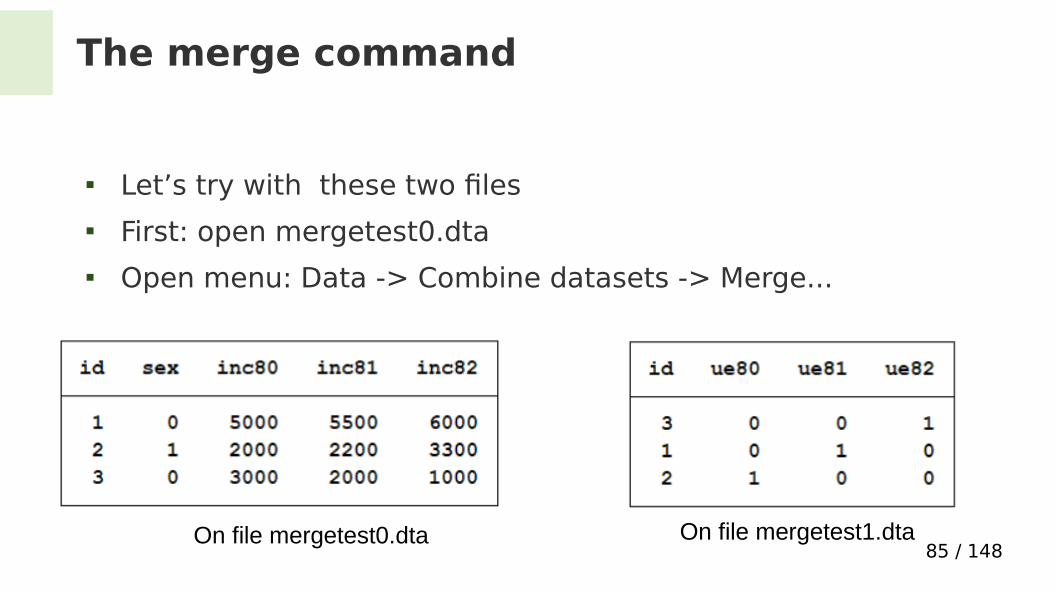
The merge command
Let’s try with these two fles First: open mergetest0.dta Open menu: Data -> Combine datasets -> Merge...
On file mergetest1.dtaOn file mergetest0.dta
86 / 148
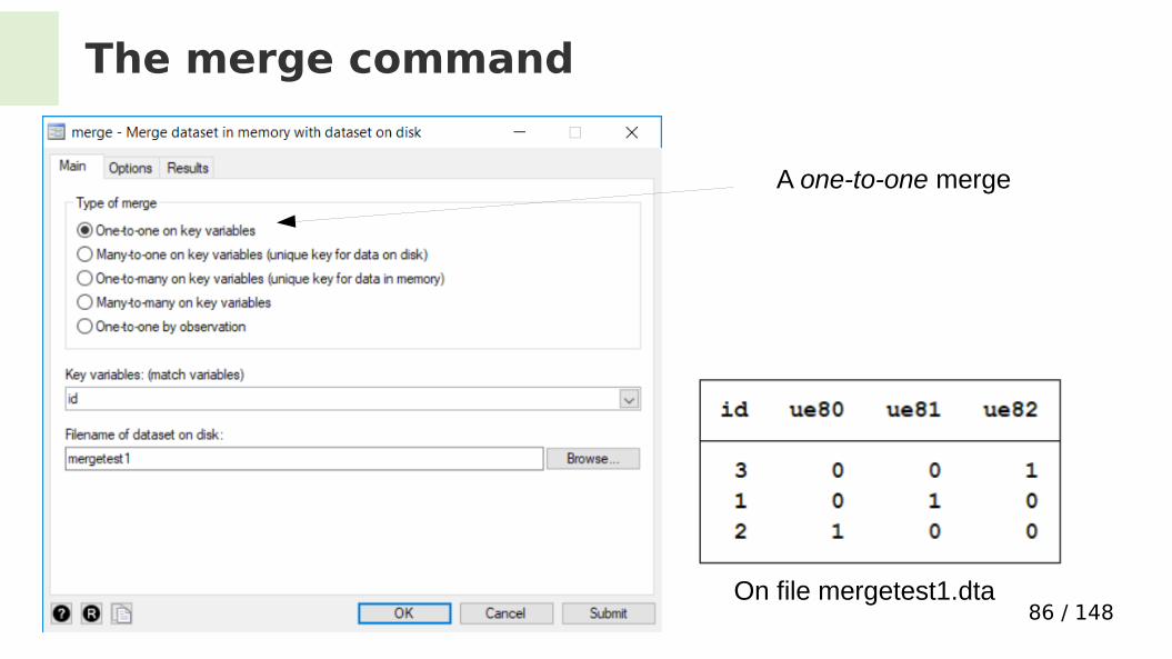
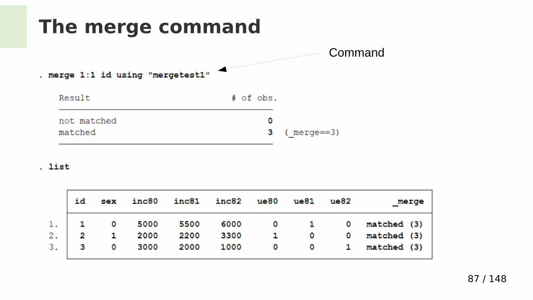
The merge command
On file mergetest1.dta
A one-to-one merge
87 / 148
The merge commandCommand
88 / 148
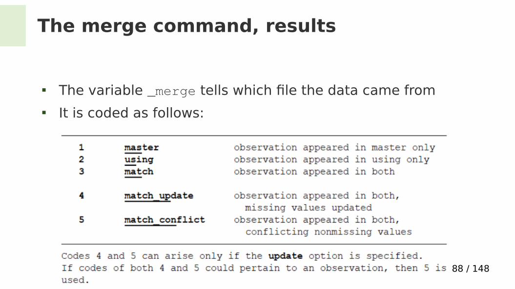
The merge command, results
The variable _merge tells which fle the data came from It is coded as follows:

89 / 148
The merge command, options
Choose variables to keep
Update from disk

90 / 148
Part 4: Descriptive statistics
‘Descriptive’ as in ‘Describing the Data’
Difers from statistical inference, which means to generalize from data (estimation, modelling...)
Let’s also include descriptive graphics!

91 / 148
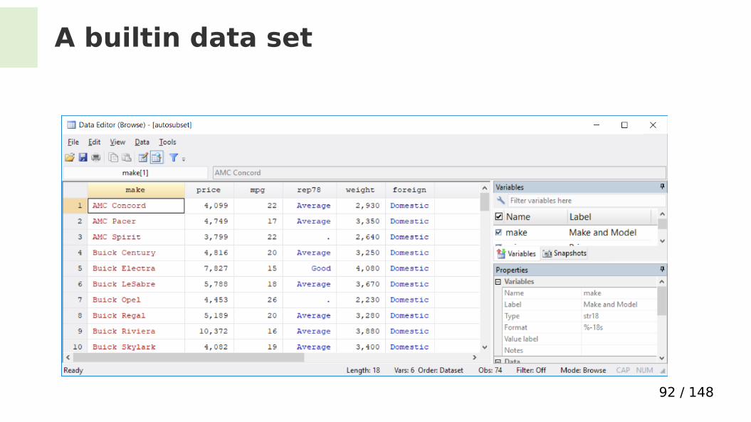
A builtin data set
sysuse auto2 open a data set that comes along with the Stata program (Menu: ‘File’ - ‘Example datasets’)
keep make price mpg rep78 weight foreign chooses a few variables
What variable types do we have now?
92 / 148
A builtin data set

93 / 148
A builtin data set
Coding of values?

94 / 148
A builtin data set
Coding of values?

95 / 148
A builtin data set
Coding of values?
96 / 148
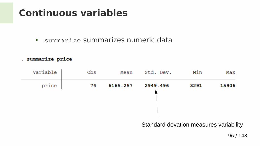
Continuous variables
summarize summarizes numeric data
Standard devation measures variability

97 / 148
Continuous variables
More than one variable can be summarized
98 / 148
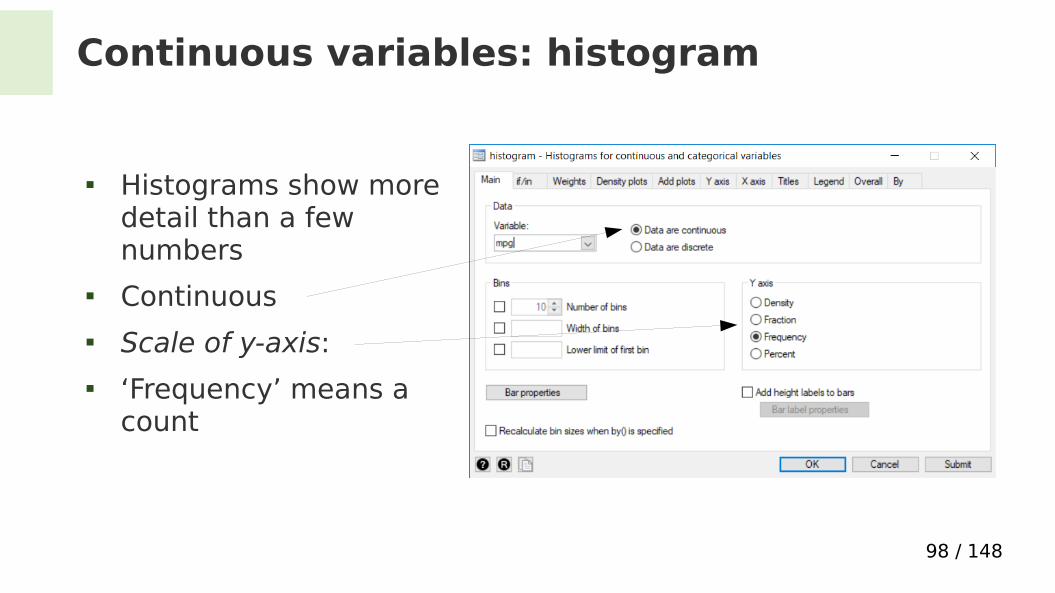
Continuous variables: histogram
Histograms show more detail than a few numbers
Continuous Scale of y-axis: ‘Frequency’ means a
count

99 / 148
Continuous variables: histogram
‘Frequency’ means a count
i.e. number of observations within an interval
Intervals (aka ‘Bins’) can be adjusted

100 / 148
Continuous variables: histogram
Graphs can be edited by clicking here
e.g. change colours, text size, graph shape

101 / 148
Continuous variables: percentiles
Percentiles can be ordered here
Median = 50%-percentile

102 / 148
Categorical variables
A frequency table Count each category

103 / 148
Categorical variables: bar chart
Choose ‘Bar Chart’ in the Graphics-menu Choose ‘frequency within categories’ Then choose a ‘grouping variable’

104 / 148
Categorical variables: bar chart
Number of cars in each group

105 / 148
Categorical variables: Ordinal
For ordinal variables we can calculate a median (but the mean makes no sense)
Command: centile rep78
106 / 148
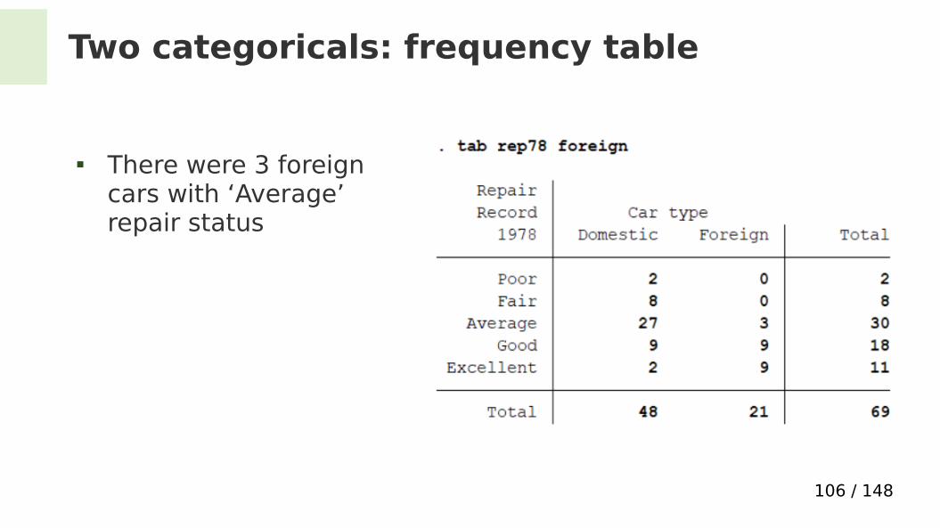
Two categoricals: frequency table
There were 3 foreign cars with ‘Average’ repair status

107 / 148
Two categoricals: frequency table
Menu has lots of options Percentage of foreign
cars in each row

108 / 148
Two categoricals: frequency table
Menu has lots of options Percentage of foreign
cars in each row

109 / 148
Two categoricals: bar chart
Tick off here to get different coloursChoose two categorical variables

110 / 148
Two categoricals: bar chart
graph bar (count), over(foreign) over(rep78) asyvars

111 / 148
One continuous and one categorical
Are American cars less efective?
mpg vs. foreign Visualize with ‘Box plot’

112 / 148
One continuous and one categorical
Continuous Categorical
113 / 148
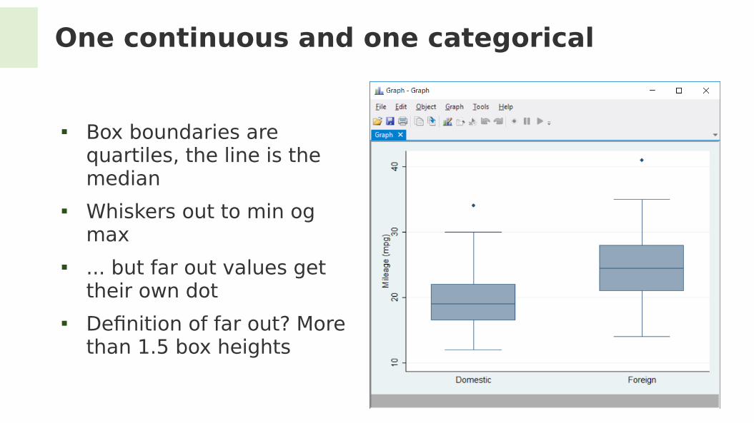
One continuous and one categorical
Box boundaries are quartiles, the line is the median
Whiskers out to min og max
... but far out values get their own dot
Defnition of far out? More than 1.5 box heights

114 / 148
Useful: by
Statistics for every category, labourious way:

115 / 148
Useful: by
Statistics for every category, more convenient:
116 / 148
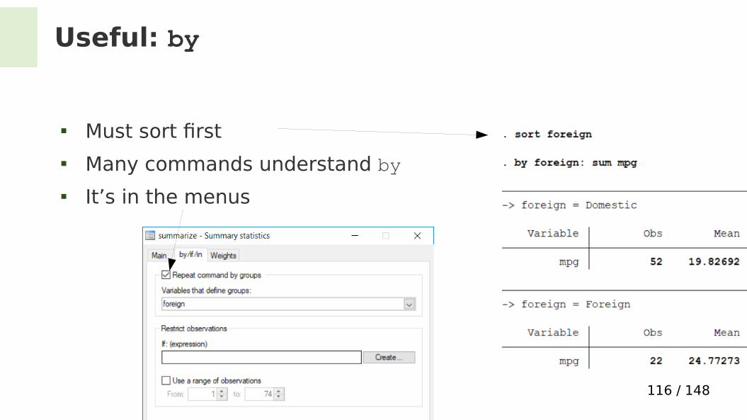
Useful: by
Must sort frst Many commands understand by It’s in the menus

117 / 148
Two continuous variables: scatterplot
Are mpg and weight associated? We can plot each data point in a 2D ‘map’

118 / 148
Two continuous variables: scatterplot
Click ‘Create’ ... which will open a
second window

119 / 148
Two continuous variables: scatterplot
Choose ‘Scatter’ Choose variables Click ‘Accept’

120 / 148
Two continuous variables: scatterplot
We’re back in the frst window
Click OK or Submit

121 / 148
Two continuous variables: scatterplot
As expected?
122 / 148
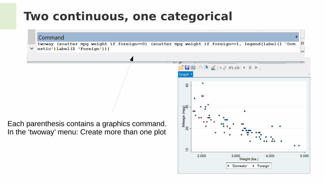
Two continuous, one categorical
Each parenthesis contains a graphics command. In the ‘twoway’ menu: Create more than one plot

124 / 148
Part 5: Estimation and testing
Estimate mean Standard error Comparing two means

125 / 148
Del 5: Estimating the mean
We want to estimate population mean We can do this with the sample mean ... if we have a representative, e.g. random, sample
2 5
4
2 7
26
6
41
5
4
Sample: 2, 2, 4, 5
Sample mean is (2+2+4+5)/4 = 3.25Population mean is 4
Estimation error is 4 - 3.25 = 0.75
126 / 148
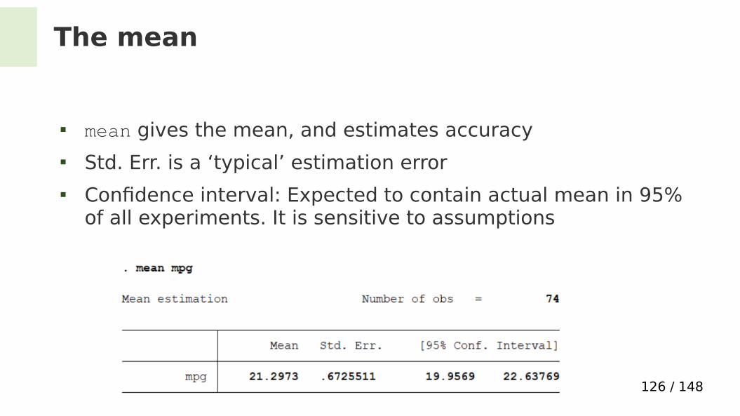
The mean
mean gives the mean, and estimates accuracy Std. Err. is a ‘typical’ estimation error Confdence interval: Expected to contain actual mean in 95%
of all experiments. It is sensitive to assumptions

127 / 148
Confdence interval
The command ci has more options for the confdence interval
The default is based on normal distribution, ci also allows binomial og Poisson distributions

128 / 148
Two means
Diferences between domestic and foreign? Let’s investigate with mean
129 / 148
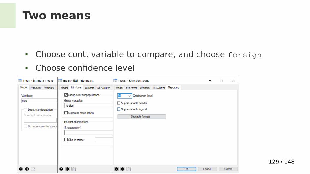
Two means
Choose cont. variable to compare, and choose foreign Choose confdence level

130 / 148
Two means
Estimates for each category Do the confdence intervals overlap?

131 / 148
Two means
What about that p-value thing?

132 / 148
Two means
A typical Stata dialogue box
Tick of here to group by a categorical variable

133 / 148
Two means: Student t-test
One- and twosided p-values
However: Normal distributions? Outliers? Equal standard deviation? Random sample?

134 / 148
Two means: Student t-test
We can, and should adjust for unequal standard deviations
However: Equal standard deviation?

135 / 148
Two means: Student t-test
Look at sample distributions with histograms Skewed for Domestic
However: Normal distributions?
Alternative test ranksum needs less assumptions (but may have less power)
Bootstrap may be useful

136 / 148
Two means: Student t-test
Let’s try a variable transformation:
generate gpm=1/mpg
Less skewed Can we compare means of
gpm instead?

137 / 148
Linear regression
Can we quantify the association between efciency and weight?
Let’s try gpm = b0 + b1 * weight + noise
138 / 148
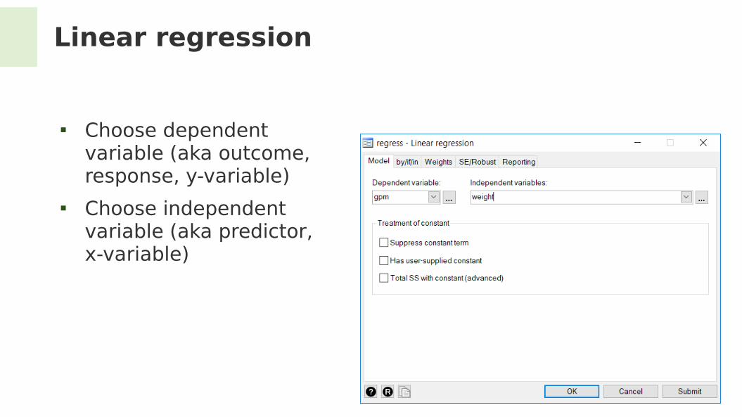
Linear regression
Choose dependent variable (aka outcome, response, y-variable)
Choose independent variable (aka predictor, x-variable)

139 / 148
Linear regression, the output
Command
How much variance does the model ‘explain’
Coefficient values with error estimates
140 / 148
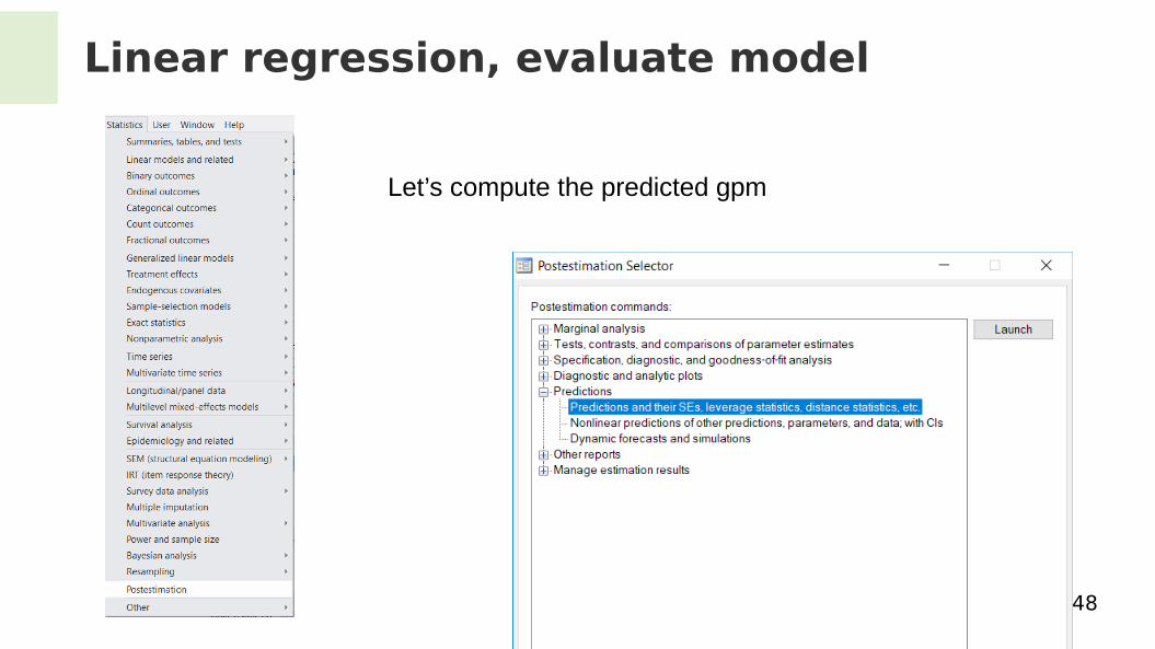
Linear regression, evaluate model
Let’s compute the predicted gpm
141 / 148
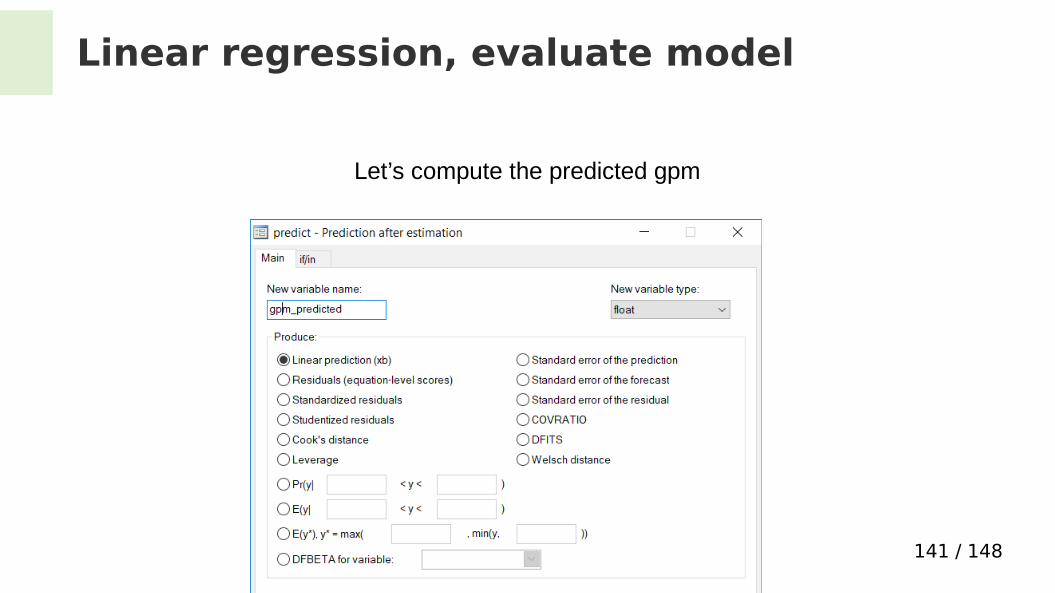
Linear regression, evaluate model
Let’s compute the predicted gpm

142 / 148
Linear regression, graph model
Plot of model and data Linearity looks reasonable Other assumptions?
(normal errors, homoskedasticity, independent samples)
twoway (line gpm_predicted weight) (scatter gpm weight)

143 / 148
Linear regression, multiple
We can have more than one predictor, e.g.
gpm = b0 + b1 * weight + b2 * foreign + noise Note that foreign is either 0 or 1 Categoricals with more than two values must be represented
with ‘indicator variables’, aka ‘dummy variables’
(although ordinals are sometimes excepted from this rule) Interpretation, visualisation etc, becomes more complicated

144 / 148
Linear regression, multiple
The Stata output looks the same, except more coefcients

145 / 148
Part 6: Where to go from here
Getting help, fnding documentation Tips about other useful commands

146 / 148
Help in Stata
If known command name: help ttest If in dialogue box: click ‘?’ If unknown command: search student t-test Google, e.g. ‘Stata t-test’ Pdf-manual of Stata is good, if technical, with nice examples.
Access via menu Or search with Google, e.g. ‘ttest site:stata.com/manuals’

147 / 148
Further reading
Acock: A gentle introduction to Stata (5th ed) Midtbø: Stata - en entusiastisk innføring Visual overview of graphics options:
https://www.stata.com/support/faqs/graphics/gph/stata-graphs/
Stata manual ch. 27: ‘Commands everyone should know’https://www.stata.com/manuals/u27.pdf
Nettskjema and Stata: https://www-adm.uio.no/tjenester/it/applikasjoner/nettskjema/hjelp/se-resultater-analyse/til-stata.html

148 / 148
Things not in these slides
Variable lists Convert between text/numbers: destring, tostring Variable transformations, for example: replace, egen, _n, _N,... Break continuous into categorical (use generate with if, or use
the egen function cut)
Various: count, display, drop, order Correlation, and much more analysis External commands
149 / 148
Help at USIT
Help with statistics/statistics programs etc
http://www.uio.no/tjenester/it/forskning/statistikk/kontakt/ Statistics mailing list: [email protected]