1

Introduction to Neural Networks

CompSci 270Ronald Parr

Duke UniversityDepartment of Computer Science

With thanks to Kris Hauser for some content

Many Applications of Neural Networks

• Used in unsupervised, supervised, and reinforcement learning

• Focus on use for supervised learning here

• Note: Not a different type of learning – just a different type of function

2

Types of Supervised Learning

• Training input:– Feature vector for each datum: x1…xn

– Target value: y

• Classification – assigning labels/classes• Regression – assigning real numbers

Features and Targets• Features can be anything

– Images, sounds, text– Real values (height, weight)– Integers, or binaries

• Targets can be discrete classes:– Safe mushrooms vs. poisonous– Malignant vs. benign– Good credit risk vs. bad– Label of image

• Or numbers– Selling price of house– Life expectancy

3

How Most Supervised Learning Algorithms Work

• Main idea: Minimize error on training set• How this is done depends on:

– Hypothesis space– Type of data

• Some approaches use a regularizer or priorto trade off training set error vs. hypothesis space complexity

Classification vs. Regression

• Regression tries to hit the target values with the function we are fitting

• Classification tries to find a function that separates the classes

4

Suppose we’re in 1-dimension

Easy to find a linear separator

x=0

Copyright © 2001, 2003, Andrew W. Moore

Harder 1-dimensional dataset

What can be done about this?

x=0

Copyright © 2001, 2003, Andrew W. Moore

5

Harder 1-dimensional dataset

Remember how permitting non-linear basis functions made linear regression so much nicer?

Let’s permit them here too

x=0

Copyright © 2001, 2003, Andrew W. Moore

Harder 1-dimensional dataset

Now linearly separable in the new feature space

But, what if the right feature set isn’t obvious

x=0

Copyright © 2001, 2003, Andrew W. Moore

6

Motivation for non-linear Classifiers

• Linear methods are “weak”– Make strong assumptions– Can only express relatively simple functions of inputs

• Coming up with good features can be hard– Requires human input– Knowledge of the domain

• Role of neural networks– Neural networks started as linear models of single neurons– Combining ultimately let to non-linear that don’t necessarily need

careful feature engineering

Neural Network Motivation

• Human brains are only known example of actual intelligence• Individual neurons are slow, boring• Brains succeed by using massive parallelism• Idea: Copy what works

• Raises many issues:– Is the computational metaphor suited to the computational hardware?– How do we know if we are copying the important part?– Are we aiming too low?

7

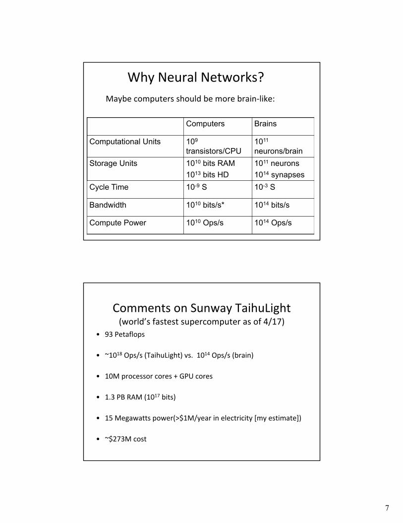
Why Neural Networks?Maybe computers should be more brain-like:

Computers Brains

Computational Units 109

transistors/CPU1011

neurons/brainStorage Units 1010 bits RAM

1013 bits HD1011 neurons1014 synapses

Cycle Time 10-9 S 10-3 S

Bandwidth 1010 bits/s* 1014 bits/s

Compute Power 1010 Ops/s 1014 Ops/s

Comments on Sunway TaihuLight(world’s fastest supercomputer as of 4/17)

• 93 Petaflops

• ~1018 Ops/s (TaihuLight) vs. 1014 Ops/s (brain)

• 10M processor cores + GPU cores

• 1.3 PB RAM (1017 bits)

• 15 Megawatts power(>$1M/year in electricity [my estimate])

• ~$273M cost

8

More Comments on Taihu Light

• What is wrong with this picture?– Weight– Size– Power Consumption

• What is missing?– Still can’t replicate human abilities

(though vastly exceeds human abilities in many areas)– Are we running the wrong programs?– Is the architecture well suited to the programs we

might need to run?

Artificial Neural Networks

• Develop abstraction of function of actual neurons

• Simulate large, massively parallel artificial neural networks on conventional computers

• Some have tried to build the hardware too

• Try to approximate human learning, robustness to noise, robustness to damage, etc.

9

Early Uses of neural networks

• Trained to pronounce English– Training set: Sliding window over text, sounds

– 95% accuracy on training set

– 78% accuracy on test set

• Trained to recognize handwritten digits– >99% accuracy

• Trained to drive (Pomerleau et al. no-hands across America 1995)

https://www.cs.cmu.edu/~tjochem/nhaa/navlab5_details.html

Neural Network Lore

• Neural nets have been adopted with an almost religious fervor within the AI community – several times– First coming: Perceptron– Second coming: Multilayer networks– Third coming (present): Deep networks

• Sound science behind neural networks: gradient descent• Unsound social phenomenon behind neural networks: HYPE!

10

Artificial Neurons

node/neuron

xj wj,i zi

!!

€

ai = h( w j,ix jj∑ )

h can be any function, but usually a smoothed step function

h

Threshold Functions

-1.5

-1

-0.5

0

0.5

1

1.5

-10 -5 0 5 10

-1

-0.5

0

0.5

1

-10 -5 0 5 10

h(x)=tanh(x) or 1/(1+exp(-x))(logistic sigmoid)

h(x)=sgn(x)(perceptron)

11

Network Architectures

• Cyclic vs. Acyclic– Cyclic is tricky, but more biologically plausible

• Hard to analyze in general• May not be stable• Need to assume latches to avoid race conditions

– Hopfield nets: special type of cyclic net useful for associative memory

• Single layer (perceptron)• Multiple layer

Feedforward Networks

• We consider acyclic networks• One or more computational layers• Entire network can be viewed as computing a complex

non-linear function• Typical uses in learning:

– Classification (usually involving complex patterns)– General continuous function approximation

12

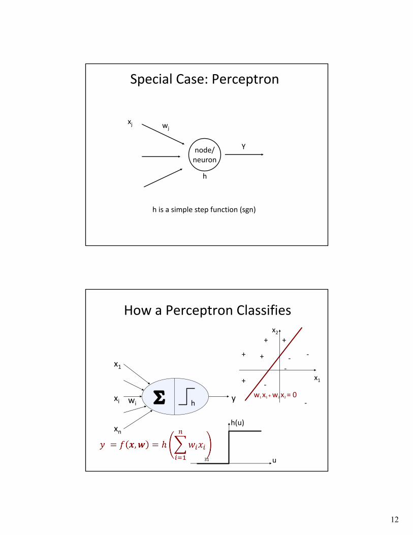
Special Case: Perceptron

node/neuron

xj wj

Y

h

h is a simple step function (sgn)

How a Perceptron Classifies

31

S hxi

x1

xn

ywi

+ +

+

++ -

-

--

-x1

x2

w1 x1 + w2 x2 = 0

h(u)

u

13

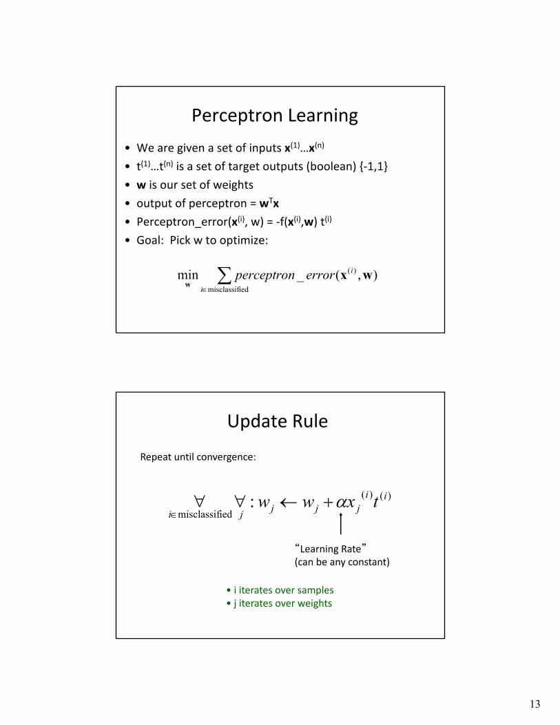
Perceptron Learning• We are given a set of inputs x(1)…x(n)

• t(1)…t(n) is a set of target outputs (boolean) {-1,1}• w is our set of weights• output of perceptron = wTx• Perceptron_error(x(i), w) = -f(x(i),w) t(i)

• Goal: Pick w to optimize:

åÎ iedmisclassif

)( ),(_mini

ierrorperceptron wxw

Update Rule

)()(

iedmisclassif: ii

jjjjitxww a+¬""

Î

Repeat until convergence:

�Learning Rate�(can be any constant)

• i iterates over samples• j iterates over weights

14

Good News/Bad News

• Good news– Perceptron can distinguish any two classes that

are linearly separable– If classes are separable, perceptron learning

rule will converge for any learning rate• Bad news

– Linear separability is a strong assumption– Failure to appreciate this led to excessive

optimism and first neural network crash

Visualizing Linearly Separable Functions

Is red linearly separable from green?Are the circles linearly separable from the squares?

15

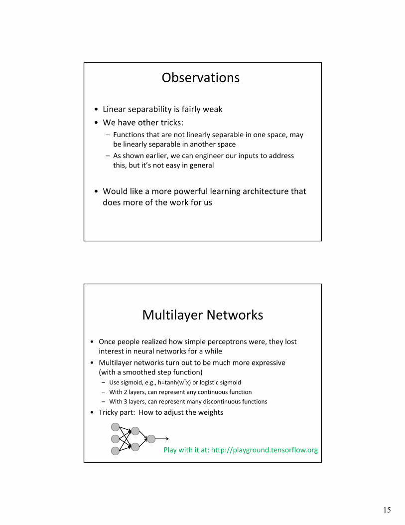
Observations

• Linear separability is fairly weak• We have other tricks:

– Functions that are not linearly separable in one space, may be linearly separable in another space

– As shown earlier, we can engineer our inputs to address this, but it’s not easy in general

• Would like a more powerful learning architecture that does more of the work for us

Multilayer Networks

• Once people realized how simple perceptrons were, they lost interest in neural networks for a while

• Multilayer networks turn out to be much more expressive(with a smoothed step function)– Use sigmoid, e.g., h=tanh(wTx) or logistic sigmoid– With 2 layers, can represent any continuous function– With 3 layers, can represent many discontinuous functions

• Tricky part: How to adjust the weights

Play with it at: http://playground.tensorflow.org

16

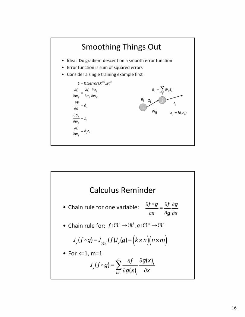
Smoothing Things Out• Idea: Do gradient descent on a smooth error function• Error function is sum of squared errors• Consider a single training example first

!!!!

€

E = 0.5error(X ( i),w)2

∂E∂wij

=∂E∂a j

∂a j

∂wij

∂E∂a j

= δ j

∂a j

∂wij

= zi

∂E∂wij

= δ jzi

ij

wij

ai!!

€

a j = wijzii∑

zi zj

!!

€

z j = h(a j)

Calculus Reminder

• Chain rule for one variable:

• Chain rule for:

• For k=1, m=1

∂f g∂x

=∂f∂g

∂g∂x

f :ℜn →ℜk ,g :ℜm →ℜn

Jx ( f !g)= Jg(x )( f )Jx (g)= k×n( ) n×m( )

Jx ( f g)=∂f

∂g(x)ii=1

n

∑∂g(x)i∂x

17

Propagating Errors

• For output units (assuming no weights on outputs)

• For hidden units!!

€

∂E∂a j

= δ j = y − t

kk

ikii

iik

k ki

k

k ki

i

wahahw

aE

aa

aE

aE dd ååå =

¶¶

¶¶

=¶¶

¶¶

==¶¶ )('

ijwijai

!!

€

a j = wijzii∑

zj=output

!!

€

z j = f (a j)

All upstream nodes from i

Chain rule

∂E∂wij

=∂E∂aj

∂aj

∂wij

=δ jzi

∂E∂aj

=δ j ,"""∂aj

∂wij

= zi ,""""

Differentiating h

• Recall the logistic sigmoid:

• Differentiating:

!!!!!!

€

h(x) =ex

1+ ex =1

1+ e−x

!!!!!!

€

1 − h(x) =e−x

1+ e−x=

11+ ex

!!!!

€

h'(x) =e−x

(1+ e−x )2=

1(1+ e−x )

e−x

(1+ e−x )= h(x)(1 − h(x))

18

Putting it together

• Apply input x to network (sum for multiple inputs)– Compute all activation levels– Compute final output (forward pass)

• Compute d for output units

• Backpropagate ds to hidden units

• Compute gradient update:

!!

€

δ = y − t

!!

€

δ j =∂E∂akk

∑ ∂ak

∂a j

= h'(a j) wkjk∑ δk

!!

€

∂E∂wij

= δ jai

Summary of Gradient Update

• Gradient calculation, parameter updates have recursive formulation

• Decomposes into:– Local message passing– No transcendentals:

• h’(x)=1-h(x)2 for tanh(x)• H’(x)=h(x)(1-h(x)) for logistic sigmoid

• Highly parallelizable• Biologically plausible(?)

• Celebrated backpropagation algorithm

19

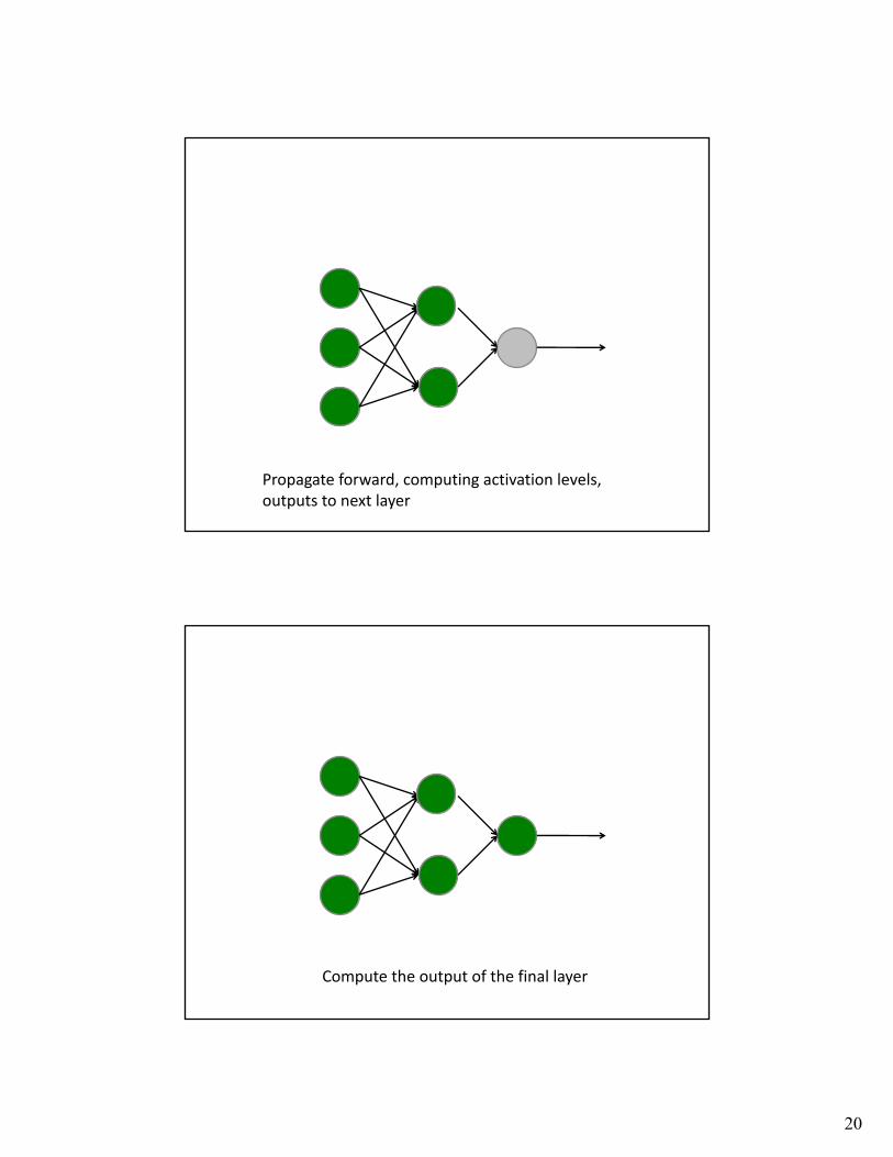
Inputs

20

Propagate forward, computing activation levels,outputs to next layer

Compute the output of the final layer

21

Compute the error (d) for the final layer

!!

€

∂E∂wij

= δ jaiCompute the error d’s and gradient updates for earlier layers:

22

Complete training for one datum – now repeat for entire training set

Good News

• Can represent any continuous function with two layers (1 hidden)

• Can represent essentially any function with 3 layers• (But how many hidden nodes?)

• Multilayer nets are a universal approximation architecture with a highly parallelizable training algorithm

23

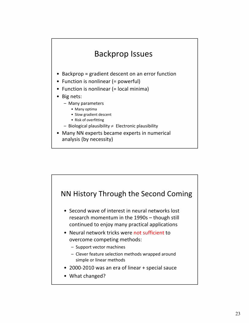
Backprop Issues

• Backprop = gradient descent on an error function• Function is nonlinear (= powerful)• Function is nonlinear (= local minima)• Big nets:

– Many parameters• Many optima• Slow gradient descent• Risk of overfitting

– Biological plausibility ¹ Electronic plausibility• Many NN experts became experts in numerical

analysis (by necessity)

NN History Through the Second Coming

• Second wave of interest in neural networks lost research momentum in the 1990s – though still continued to enjoy many practical applications

• Neural network tricks were not sufficient to overcome competing methods:– Support vector machines– Clever feature selection methods wrapped around

simple or linear methods• 2000-2010 was an era of linear + special sauce• What changed?

24

Deep Networks

• Not a learning algorithm, but a family of techniques– Improved training techniques (though still essentially gradient descent)– Clever crafting of network structure – convolutional nets

• Exploit massive computational power– Parallel computing– GPU computing– Very large data sets (can reduce overfitting)

Deep Networks Today

• Still on the upward swing of the hype pendulum• State of the art performance for many tasks:

– Speech recognition– Object recognition– Playing video games

• Controversial:– Hype, hype, hype! (but it really does work well in many cases!)– Theory lags practice– Collection of tricks, not an entirely a science yet– Results are not human-interpretable

25

Conclusions

• Neural nets = general function approximation architecture

• Gradient decomposition permits parallelizable training

• Historically wild swings in popularity

• Currently on upswing due to clever changes in training methods, use of parallel computation, and large data sets