1

INTRODUCTION TO MULTIPHASE FLOW

1.1 INTRODUCTION

1.1.1 Scope

In the context of this book, the term multiphase flow is used to refer toany fluid flow consisting of more than one phase or component. For brevityand because they are covered in other texts, we exclude those circumstancesin which the components are well mixed above the molecular level. Conse-quently, the flows considered here have some level of phase or componentseparation at a scale well above the molecular level. This still leaves anenormous spectrum of different multiphase flows. One could classify themaccording to the state of the different phases or components and thereforerefer to gas/solids flows, or liquid/solids flows or gas/particle flows or bubblyflows and so on; many texts exist that limit their attention in this way. Sometreatises are defined in terms of a specific type of fluid flow and deal withlow Reynolds number suspension flows, dusty gas dynamics and so on. Oth-ers focus attention on a specific application such as slurry flows, cavitatingflows, aerosols, debris flows, fluidized beds and so on; again there are manysuch texts. In this book we attempt to identify the basic fluid mechanicalphenomena and to illustrate those phenomena with examples from a broadrange of applications and types of flow.

Parenthetically, it is valuable to reflect on the diverse and ubiquitous chal-lenges of multiphase flow. Virtually every processing technology must dealwith multiphase flow, from cavitating pumps and turbines to electropho-tographic processes to papermaking to the pellet form of almost all rawplastics. The amount of granular material, coal, grain, ore, etc. that is trans-ported every year is enormous and, at many stages, that material is requiredto flow. Clearly the ability to predict the fluid flow behavior of these pro-cesses is central to the efficiency and effectiveness of those processes. For

19

example, the effective flow of toner is a major factor in the quality and speedof electrophotographic printers. Multiphase flows are also a ubiquitous fea-ture of our environment whether one considers rain, snow, fog, avalanches,mud slides, sediment transport, debris flows, and countless other naturalphenomena to say nothing of what happens beyond our planet. Very criticalbiological and medical flows are also multiphase, from blood flow to semento the bends to lithotripsy to laser surgery cavitation and so on. No singlelist can adequately illustrate the diversity and ubiquity; consequently anyattempt at a comprehensive treatment of multiphase flows is flawed unlessit focuses on common phenomenological themes and avoids the temptationto digress into lists of observations.

Two general topologies of multiphase flow can be usefully identified atthe outset, namely disperse flows and separated flows. By disperse flowswe mean those consisting of finite particles, drops or bubbles (the dispersephase) distributed in a connected volume of the continuous phase. On theother hand separated flows consist of two or more continuous streams ofdifferent fluids separated by interfaces.

1.1.2 Multiphase flow models

A persistent theme throughout the study of multiphase flows is the need tomodel and predict the detailed behavior of those flows and the phenomenathat they manifest. There are three ways in which such models are explored:(1) experimentally, through laboratory-sized models equipped with appro-priate instrumentation, (2) theoretically, using mathematical equations andmodels for the flow, and (3) computationally, using the power and size ofmodern computers to address the complexity of the flow. Clearly there aresome applications in which full-scale laboratory models are possible. But,in many instances, the laboratory model must have a very different scalethan the prototype and then a reliable theoretical or computational modelis essential for confident extrapolation to the scale of the prototype. Thereare also cases in which a laboratory model is impossible for a wide varietyof reasons.

Consequently, the predictive capability and physical understanding mustrely heavily on theoretical and/or computational models and here the com-plexity of most multiphase flows presents a major hurdle. It may be possibleat some distant time in the future to code the Navier-Stokes equations foreach of the phases or components and to compute every detail of a multi-phase flow, the motion of all the fluid around and inside every particle ordrop, the position of every interface. But the computer power and speed

20

required to do this is far beyond present capability for most of the flowsthat are commonly experienced. When one or both of the phases becomesturbulent (as often happens) the magnitude of the challenge becomes trulyastronomical. Therefore, simplifications are essential in realistic models ofmost multiphase flows.

In disperse flows two types of models are prevalent, trajectory models andtwo-fluid models. In trajectory models, the motion of the disperse phase isassessed by following either the motion of the actual particles or the motionof larger, representative particles. The details of the flow around each of theparticles are subsumed into assumed drag, lift and moment forces acting onand altering the trajectory of those particles. The thermal history of theparticles can also be tracked if it is appropriate to do so. Trajectory mod-els have been very useful in studies of the rheology of granular flows (seechapter 13) primarily because the effects of the interstitial fluid are small. Inthe alternative approach, two-fluid models, the disperse phase is treated asa second continuous phase intermingled and interacting with the continuousphase. Effective conservation equations (of mass, momentum and energy) aredeveloped for the two fluid flows; these included interaction terms modelingthe exchange of mass, momentum and energy between the two flows. Theseequations are then solved either theoretically or computationally. Thus, thetwo-fluid models neglect the discrete nature of the disperse phase and ap-proximate its effects upon the continuous phase. Inherent in this approach,are averaging processes necessary to characterize the properties of the dis-perse phase; these involve significant difficulties. The boundary conditionsappropriate in two-fluid models also pose difficult modeling issues.

In contrast, separated flows present many fewer issues. In theory one mustsolve the single phase fluid flow equations in the two streams, coupling themthrough appropriate kinematic and dynamic conditions at the interface. Freestreamline theory (see, for example, Birkhoff and Zarantonello 1957, Tulin1964, Woods 1961, Wu 1972) is an example of a successful implementationof such a strategy though the interface conditions used in that context areparticularly simple.

In the first part of this book, the basic tools for both trajectory andtwo-fluid models are developed and discussed. In the remainder of this firstchapter, a basic notation for multiphase flow is developed and this leadsnaturally into a description of the mass, momentum and energy equationsapplicable to multiphase flows, and, in particular, in two-fluid models. Inchapters 2, 3 and 4, we examine the dynamics of individual particles, dropsand bubbles. In chapter 7 we address the different topologies of multiphase

21

flows and, in the subsequent chapters, we examine phenomena in whichparticle interactions and the particle-fluid interactions modify the flow.

1.1.3 Multiphase flow notation

The notation that will be used is close to the standard described by Wallis(1969). It has however been slightly modified to permit more ready adop-tion to the Cartesian tensor form. In particular the subscripts that can beattached to a property will consist of a group of uppercase subscripts fol-lowed by lowercase subscripts. The lower case subscripts (i, ij, etc.) areused in the conventional manner to denote vector or tensor components. Asingle uppercase subscript (N ) will refer to the property of a specific phaseor component. In some contexts generic subscripts N = A,B will be usedfor generality. However, other letters such as N = C (continuous phase),N = D (disperse phase), N = L (liquid), N = G (gas), N = V (vapor) orN = S (solid) will be used for clarity in other contexts. Finally two upper-case subscripts will imply the difference between the two properties for thetwo single uppercase subscripts.

Specific properties frequently used are as follows. Volumetric fluxes (vol-ume flow per unit area) of individual components will be denoted by jAi, jBi

(i = 1, 2 or 3 in three dimensional flow). These are sometimes referred to assuperficial component velocities. The total volumetric flux, ji is then givenby

ji = jAi + jBi + . . . =∑N

jNi (1.1)

Mass fluxes are similarly denoted by GAi, GBi or Gi. Thus if the densitiesof individual components are denoted by ρA, ρB it follows that

GAi = ρAjAi ; GBi = ρBjBi ; Gi =∑N

ρN jNi (1.2)

Velocities of the specific phases are denoted by uAi, uBi or, in general, byuNi. The relative velocity between the two phases A and B will be denotedby uABi such that

uAi − uBi = uABi (1.3)

The volume fraction of a component or phase is denoted by αN and, inthe case of two components or phases, A and B, it follows that αB = 1 −αA. Though this is clearly a well defined property for any finite volume inthe flow, there are some substantial problems associated with assigning a

22

value to an infinitesimal volume or point in the flow. Provided these canbe resolved, it follows that the volumetric flux of a component, N , and itsvelocity are related by

jNi = αNuNi (1.4)

and that

ji = αAuAi + αBuBi + . . .=∑N

αNuNi (1.5)

Two other fractional properties are only relevant in the context of one-dimensional flows. The volumetric quality, βN , is the ratio of the volumetricflux of the component, N , to the total volumetric flux, i.e.

βN = jN/j (1.6)

where the index i has been dropped from jN and j because β is only used inthe context of one-dimensional flows and the jN , j refer to cross-sectionallyaveraged quantities.

The mass fraction, xA, of a phase or component, A, is simply given byρAαA/ρ (see equation 1.8 for ρ). On the other hand the mass quality, XA,is often referred to simply as the quality and is the ratio of the mass flux ofcomponent, A, to the total mass flux, or

XA =GA

G=

ρAjA∑NρNjN

(1.7)

Furthermore, when only two components or phases are present it is oftenredundant to use subscripts on the volume fraction and the qualities sinceαA = 1 − αB, βA = 1 − βB and XA = 1− XB . Thus unsubscripted quanti-ties α, β and X will often be used in these circumstances.

It is clear that a multiphase mixture has certain mixture properties ofwhich the most readily evaluated is the mixture density denoted by ρ andgiven by

ρ =∑N

αNρN (1.8)

On the other hand the specific enthalpy, h, and specific entropy, s, beingdefined as per unit mass rather than per unit volume are weighted accordingto

ρh =∑N

ρNαNhN ; ρs =∑N

ρNαNsN (1.9)

23

Other properties such as the mixture viscosity or thermal conductivity can-not be reliably obtained from such simple weighted means.

Aside from the relative velocities between phases that were described ear-lier, there are two other measures of relative motion that are frequentlyused. The drift velocity of a component is defined as the velocity of thatcomponent in a frame of reference moving at a velocity equal to the totalvolumetric flux, ji, and is therefore given by, uNJi, where

uNJi = uNi − ji (1.10)

Even more frequent use will be made of the drift flux of a component whichis defined as the volumetric flux of a component in the frame of referencemoving at ji. Denoted by jNJi this is given by

jNJi = jNi − αN ji = αN (uNi − ji) = αNuNJi (1.11)

It is particularly important to notice that the sum of all the drift fluxes mustbe zero since from equation 1.11∑

N

jNJi =∑N

jNi − ji∑N

αN = ji − ji = 0 (1.12)

When only two phases or components, A and B, are present it follows thatjAJi = −jBJi and hence it is convenient to denote both of these drift fluxesby the vector jABi where

jABi = jAJi = −jBJi (1.13)

Moreover it follows from 1.11 that

jABi = αAαBuABi = αA(1− αA)uABi (1.14)

and hence the drift flux, jABi and the relative velocity, uABi, are simplyrelated.

Finally, it is clear that certain basic relations follow from the above def-initions and it is convenient to identify these here for later use. First therelations between the volume and mass qualities that follow from equations1.6 and 1.7 only involve ratios of the densities of the components:

XA = βA/∑N

(ρN

ρA

)βN ; βA = XA/

∑N

(ρA

ρN

)XN (1.15)

On the other hand the relation between the volume fraction and the volumequality necessarily involves some measure of the relative motion betweenthe phases (or components). The following useful results for two-phase (or

24

two-component) one-dimensional flows can readily be obtained from 1.11and 1.6

βN = αN +jNJ

j; βA = αA +

jAB

j; βB = αB − jAB

j(1.16)

which demonstrate the importance of the drift flux as a measure of therelative motion.

1.1.4 Size distribution functions

In many multiphase flow contexts we shall make the simplifying assumptionthat all the disperse phase particles (bubbles, droplets or solid particles)have the same size. However in many natural and technological processes itis necessary to consider the distribution of particle size. One fundamentalmeasure of this is the size distribution function, N (v), defined such thatthe number of particles in a unit volume of the multiphase mixture withvolume between v and v + dv is N (v)dv. For convenience, it is often assumedthat the particles size can be represented by a single linear dimension (forexample, the diameter, D, or radius, R, in the case of spherical particles) sothat alternative size distribution functions, N ′(D) or N ′′(R), may be used.Examples of size distribution functions based on radius are shown in figures1.1 and 1.2.

Often such information is presented in the form of cumulative numberdistributions. For example the cumulative distribution, N ∗(v∗), defined as

N ∗(v∗) =∫ v∗

0N (v)dv (1.17)

is the total number of particles of volume less than v∗. Examples of cumu-lative distributions (in this case for coal slurries) are shown in figure 1.3.

In these disperse flows, the evaluation of global quantities or characteris-tics of the disperse phase will clearly require integration over the full rangeof particle sizes using the size distribution function. For example, the volumefraction of the disperse phase, αD, is given by

αD =∫ ∞

0v N (v)dv =

π

6

∫ ∞

0D3 N ′(D)dD (1.18)

where the last expression clearly applies to spherical particles. Other prop-erties of the disperse phase or of the interactions between the disperse andcontinuous phases can involve other moments of the size distribution func-tion (see, for example, Friedlander 1977). This leads to a series of mean

25

Figure 1.1. Measured size distribution functions for small bubbles in threedifferent water tunnels (Peterson et al. 1975, Gates and Bacon 1978, Katz1978) and in the ocean off Los Angeles, Calif. (O’Hern et al. 1985).

Figure 1.2. Size distribution functions for bubbles in freshly poured Guin-ness and after five minutes. Adapted from Kawaguchi and Maeda (2003).

26

Figure 1.3. Cumulative size distributions for various coal slurries.Adapted from Shook and Roco (1991).

diameters (or sizes in the case of non-spherical particles) of the form, Djk,where

Djk =

[∫∞0 Dj N ′(D)dD∫∞0 Dk N ′(D)dD

] 1j−k

(1.19)

A commonly used example is the mass mean diameter, D30. On the otherhand processes that are controlled by particle surface area would be char-acterized by the surface area mean diameter, D20. The surface area meandiameter would be important, for example, in determining the exchange ofheat between the phases or the rates of chemical interaction at the dispersephase surface. Another measure of the average size that proves useful incharacterizing many disperse particulates is the Sauter mean diameter, D32.This is a measure of the ratio of the particle volume to the particle sur-face area and, as such, is often used in characterizing particulates (see, forexample, chapter 14).

1.2 EQUATIONS OF MOTION

1.2.1 Averaging

In the section 1.1.3 it was implicitly assumed that there existed an infinites-imal volume of dimension, ε, such that ε was not only very much smallerthan the typical distance over which the flow properties varied significantlybut also very much larger than the size of the individual phase elements (thedisperse phase particles, drops or bubbles). The first condition is necessaryin order to define derivatives of the flow properties within the flow field.The second is necessary in order that each averaging volume (of volume ε3)

27

contain representative samples of each of the components or phases. In thesections that follow (sections 1.2.2 to 1.2.9), we proceed to develop the ef-fective differential equations of motion for multiphase flow assuming thatthese conditions hold.

However, one of the more difficult hurdles in treating multiphase flows,is that the above two conditions are rarely both satisfied. As a consequencethe averaging volumes contain a finite number of finite-sized particles andtherefore flow properties such as the continuous phase velocity vary signifi-cantly from point to point within these averaging volumes. These variationspose the challenge of how to define appropriate average quantities in theaveraging volume. Moreover, the gradients of those averaged flow propertiesappear in the equations of motion that follow and the mean of the gradientis not necessarily equal to the gradient of the mean. These difficulties willbe addressed in section 1.4 after we have explored the basic structure of theequations in the absence of such complications.

1.2.2 Continuum equations for conservation of mass

Consider now the construction of the effective differential equations of mo-tion for a disperse multiphase flow (such as might be used in a two-fluidmodel) assuming that an appropriate elemental volume can be identified.For convenience this elemental volume is chosen to be a unit cube withedges parallel to the x1, x2, x3 directions. The mass flow of component Nthrough one of the faces perpendicular to the i direction is given by ρN jNi

and therefore the net outflow of mass of component N from the cube is givenby the divergence of ρNjNi or

∂(ρNjNi)∂xi

(1.20)

The rate of increase of the mass of component N stored in the elementalvolume is ∂(ρNαN )/∂t and hence conservation of mass of component Nrequires that

∂

∂t(ρNαN ) +

∂(ρNjNi)∂xi

= IN (1.21)

where IN is the rate of transfer of mass to the phaseN from the other phasesper unit total volume. Such mass exchange would result from a phase changeor chemical reaction. This is the first of several phase interaction terms thatwill be identified and, for ease of reference, the quantities IN will termedthe mass interaction terms.

28

Clearly there will be a continuity equation like 1.21 for each phase orcomponent present in the flow. They will referred to as the Individual PhaseContinuity Equations (IPCE). However, since mass as a whole must be con-served whatever phase changes or chemical reactions are happening it followsthat ∑

N

IN = 0 (1.22)

and hence the sum of all the IPCEs results in a Combined Phase ContinuityEquation (CPCE) that does not involve IN :

∂

∂t

(∑N

ρNαN

)+

∂

∂xi

(∑N

ρNjNi

)= 0 (1.23)

or using equations 1.4 and 1.8:

∂ρ

∂t+

∂

∂xi

(∑N

ρNαNuNi

)= 0 (1.24)

Notice that only under the conditions of zero relative velocity in which uNi =ui does this reduce to the Mixture Continuity Equation (MCE) which isidentical to that for an equivalent single phase flow of density ρ:

∂ρ

∂t+

∂

∂xi(ρui) = 0 (1.25)

We also record that for one-dimensional duct flow the individual phasecontinuity equation 1.21 becomes

∂

∂t(ρNαN ) +

1A

∂

∂x(AρNαNuN) = IN (1.26)

where x is measured along the duct, A(x) is the cross-sectional area, uN , αN

are cross-sectionally averaged quantities and AIN is the rate of transferof mass to the phase N per unit length of the duct. The sum over theconstituents yields the combined phase continuity equation

∂ρ

∂t+

1A

∂

∂x

(A∑N

ρNαNun

)= 0 (1.27)

When all the phases travel at the same speed, uN = u, this reduces to

∂ρ

∂t+

1A

∂

∂x(ρAu) = 0 (1.28)

Finally we should make note of the form of the equations when the twocomponents or species are intermingled rather than separated since we will

29

analyze several situations with gases diffusing through one another. Thenboth components occupy the entire volume and the void fractions are effec-tively unity so that the continuity equation 1.21 becomes:

∂ρN

∂t+∂(ρNuNi)

∂xi= IN (1.29)

1.2.3 Disperse phase number continuity

Complementary to the equations of conservation of mass are the equationsgoverning the conservation of the number of bubbles, drops, particles, etc.that constitute a disperse phase. If no such particles are created or destroyedwithin the elemental volume and if the number of particles of the dispersecomponent, D, per unit total volume is denoted by nD, it follows that

∂nD

∂t+

∂

∂xi(nDuDi) = 0 (1.30)

This will be referred to as the Disperse Phase Number Equation (DPNE).If the volume of the particles of component D is denoted by vD it follows

that

αD = nDvD (1.31)

and substituting this into equation 1.21 one obtains

∂

∂t(nDρDvD) +

∂

∂xi(nDuDiρDvD) = ID (1.32)

Expanding this equation using equation 1.30 leads to the following relationfor ID:

ID = nD

(∂(ρDvD)

∂t+ uDi

∂(ρDvD)∂xi

)= nD

DD

DDt(ρDvD) (1.33)

where DD/DDt denotes the Lagrangian derivative following the dispersephase. This demonstrates a result that could, admittedly, be assumed, apriori. Namely that the rate of transfer of mass to the component D in eachparticle, ID/nD, is equal to the Lagrangian rate of increase of mass, ρDvD,of each particle.

It is sometimes convenient in the study of bubbly flows to write the bubblenumber conservation equation in terms of a population, η, of bubbles perunit liquid volume rather than the number per unit total volume, nD . Note

30

that if the bubble volume is v and the volume fraction is α then

η =nD

(1 − α); nD =

η

(1 + ηv); α = η

v

(1 + ηv)(1.34)

and the bubble number conservation equation can be written as

∂uDi

∂xi= −(1 + ηv)

η

DD

DDt

(η

1 + ηv

)(1.35)

If the number population, η, is assumed uniform and constant (which re-quires neglect of slip and the assumption of liquid incompressibility) thenequation 1.35 can be written as

∂uDi

∂xi=

η

1 + ηv

DDv

DDt(1.36)

In other words the divergence of the velocity field is directly related to theLagrangian rate of change in the volume of the bubbles.

1.2.4 Fick’s law

We digress briefly to complete the kinematics of two interdiffusing gases.Equation 1.29 represented the conservation of mass for the two gases inthese circumstances. The kinematics are then completed by a statement ofFick’s Law which governs the interdiffusion. For the gas, A, this law is

uAi = ui − ρD

ρA

∂

∂xi

(ρA

ρ

)(1.37)

where D is the diffusivity.

1.2.5 Continuum equations for conservation of momentum

Continuing with the development of the differential equations, the next stepis to apply the momentum principle to the elemental volume. Prior to do-ing so we make some minor modifications to that control volume in orderto avoid some potential difficulties. Specifically we deform the boundingsurfaces so that they never cut through disperse phase particles but every-where are within the continuous phase. Since it is already assumed that thedimensions of the particles are very small compared with the dimensions ofthe control volume, the required modification is correspondingly small. Itis possible to proceed without this modification but several complicationsarise. For example, if the boundaries cut through particles, it would then benecessary to determine what fraction of the control volume surface is acted

31

upon by tractions within each of the phases and to face the difficulty of de-termining the tractions within the particles. Moreover, we shall later need toevaluate the interacting force between the phases within the control volumeand this is complicated by the issue of dealing with the parts of particlesintersected by the boundary.

Now proceeding to the application of the momentum theorem for eitherthe disperse (N = D) or continuous phase (N = C), the flux of momentumof the N component in the k direction through a side perpendicular to thei direction is ρNjNiuNk and hence the net flux of momentum (in the k di-rection) out of the elemental volume is ∂(ρNαNuNiuNk)/∂xi. The rate ofincrease of momentum of component N in the k direction within the ele-mental volume is ∂(ρNαNuNk)/∂t. Thus using the momentum conservationprinciple, the net force in the k direction acting on the component N in thecontrol volume (of unit volume), FT

Nk, must be given by

FTNk =

∂

∂t(ρNαNuNk) +

∂

∂xi(ρNαNuNiuNk) (1.38)

It is more difficult to construct the forces, FTNk in order to complete the

equations of motion. We must include body forces acting within the controlvolume, the force due to the pressure and viscous stresses on the exterior ofthe control volume, and, most particularly, the force that each componentimposes on the other components within the control volume.

The first contribution is that due to an external force field on the compo-nent N within the control volume. In the case of gravitational forces, this isclearly given by

αNρNgk (1.39)

where gk is the component of the gravitational acceleration in the k direction(the direction of g is considered vertically downward).

The second contribution, namely that due to the tractions on the controlvolume, differs for the two phases because of the small deformation discussedabove. It is zero for the disperse phase. For the continuous phase we definethe stress tensor, σCki, so that the contribution from the surface tractionsto the force on that phase is

∂σCki

∂xi(1.40)

For future purposes it is also convenient to decompose σCki into a pressure,pC = p, and a deviatoric stress, σD

Cki:

σCki = −pδki + σDCki (1.41)

32

where δki is the Kronecker delta such that δki = 1 for k = i and δij = 0 fork �= i.

The third contribution to FTNk is the force (per unit total volume) imposed

on the component N by the other components within the control volume.We write this as FNk so that the Individual Phase Momentum Equation(IPME) becomes

∂

∂t(ρNαNuNk) +

∂

∂xi(ρNαNuNiuNk)

= αNρNgk + FNk − δN

{∂p

∂xk− ∂σD

Cki

∂xi

}(1.42)

where δD = 0 for the disperse phase and δC = 1 for the continuous phase.Thus we identify the second of the interaction terms, namely the force

interaction, FNk. Note that, as in the case of the mass interaction IN , itmust follow that ∑

N

FNk = 0 (1.43)

In disperse flows it is often useful to separate FNk into two components, onedue to the pressure gradient in the continuous phase, −αD∂p/∂xk, and theremainder, F ′

Dk, due to other effects such as the relative motion betweenthe phases. Then

FDk = −FCk = −αD∂p

∂xk+ F ′

Dk (1.44)

The IPME 1.42 are frequently used in a form in which the terms on theleft hand side are expanded and use is made of the continuity equation1.21. In single phase flow this yields a Lagrangian time derivative of thevelocity on the left hand side. In the present case the use of the continuityequation results in the appearance of the mass interaction, IN . Specifically,one obtains

ρNαN

{∂uNk

∂t+ uNi

∂uNk

∂xi

}

= αNρNgk + FNk − INuNk − δN

{∂p

∂xk− ∂σD

Cki

∂xi

}(1.45)

Viewed from a Lagrangian perspective, the left hand side is the normal rateof increase of the momentum of the component N ; the term INuNk is the

33

rate of increase of the momentum in the component N due to the gain ofmass by that phase.

If the momentum equations 1.42 for each of the components are addedtogether the resulting Combined Phase Momentum Equation (CPME) be-comes

∂

∂t

(∑N

ρNαNuNk

)+

∂

∂xi

(∑N

ρNαNuNiuNk

)

= ρgk − ∂p

∂xk+∂σD

Cki

∂xi(1.46)

Note that this equation 1.46 will only reduce to the equation of motionfor a single phase flow in the absence of relative motion, uCk = uDk. Notealso that, in the absence of any motion (when the deviatoric stress is zero),equation 1.46 yields the appropriate hydrostatic pressure gradient ∂p/∂xk =ρgk based on the mixture density, ρ.

Another useful limit is the case of uniform and constant sedimentationof the disperse component (volume fraction, αD = α = 1 − αC) through thecontinuous phase under the influence of gravity. Then equation 1.42 yields

0 = αρDgk + FDk

0 =∂σCki

∂xi+ (1− α)ρCgk + FCk (1.47)

But FDk = −FCk and, in this case, the deviatoric part of the continuousphase stress should be zero (since the flow is a simple uniform stream) sothat σCkj = −p. It follows from equation 1.47 that

FDk = −FCk = −αρDgk and ∂p/∂xk = ρgk (1.48)

or, in words, the pressure gradient is hydrostatic.Finally, note that the equivalent one-dimensional or duct flow form of the

IPME is

∂

∂t(ρNαNuN) +

1A

∂

∂x

(AρNαNu

2N

)= −δN

{∂p

∂x+PτwA

}+ αNρNgx + FNx

(1.49)where, in the usual pipe flow notation, P (x) is the perimeter of the cross-section and τw is the wall shear stress. In this equation, AFNx is the forceimposed on the component N in the x direction by the other componentsper unit length of the duct. A sum over the constituents yields the combined

34

phase momentum equation for duct flow, namely

∂

∂t

(∑N

ρNαNuN

)+

1A

∂

∂x

(A∑N

ρNαNu2N

)= −∂p

∂x− Pτw

A+ ρgx (1.50)

and, when all phases travel at the same velocity, u = uN , this reduces to

∂

∂t(ρu) +

1A

∂

∂x

(Aρu2

)= −∂p

∂x− Pτw

A+ ρgx (1.51)

1.2.6 Disperse phase momentum equation

At this point we should consider the relation between the equation of mo-tion for an individual particle of the disperse phase and the Disperse PhaseMomentum Equation (DPME) delineated in the last section. This relationis analogous to that between the number continuity equation and the Dis-perse Phase Continuity Equation (DPCE). The construction of the equationof motion for an individual particle in an infinite fluid medium will be dis-cussed at some length in chapter 2. It is sufficient at this point to recognizethat we may write Newton’s equation of motion for an individual particleof volume vD in the form

DD

DDt(ρDvDuDk) = Fk + ρDvDgk (1.52)

where DD/DDt is the Lagrangian time derivative following the particle sothat

DD

DDt≡ ∂

∂t+ uDi

∂

∂xi(1.53)

and Fk is the force that the surrounding continuous phase imparts to theparticle in the direction k. Note that Fk will include not only the force dueto the velocity and acceleration of the particle relative to the fluid but alsothe buoyancy forces due to pressure gradients within the continuous phase.Expanding 1.52 and using the expression 1.33 for the mass interaction, ID,one obtains the following form of the DPME:

ρDvD

{∂uDk

∂t+ uDi

∂uDk

∂xi

}+ uDk

ID

nD= Fk + ρDvDgk (1.54)

Now examine the implication of this relation when considered alongsidethe IPME 1.45 for the disperse phase. Setting αD = nDvD in equation 1.45,expanding and comparing the result with equation 1.54 (using the continuity

35

equation 1.21) one observes that

FDk = nDFk (1.55)

Hence the appropriate force interaction term in the disperse phase momen-tum equation is simply the sum of the fluid forces acting on the individualparticles in a unit volume, namely nDFk. As an example note that thesteady, uniform sedimentation interaction force FDk given by equation 1.48,when substituted into equation 1.55, leads to the result Fk = −ρDvDgk or,in words, a fluid force on an individual particle that precisely balances theweight of the particle.

1.2.7 Comments on disperse phase interaction

In the last section the relation between the force interaction term, FDk,and the force, Fk, acting on an individual particle of the disperse phase wasestablished. In chapter 2 we include extensive discussions of the forces actingon a single particle moving in a infinite fluid. Various forms of the fluid force,Fk, acting on the particle are presented (for example, equations 2.47, 2.49,2.50, 2.67, 2.71, 3.20) in terms of (a) the particle velocity, Vk = uDk, (b) thefluid velocity Uk = uCk that would have existed at the center of the particlein the latter’s absence and (c) the relative velocity Wk = Vk − Uk.

Downstream of some disturbance that creates a relative velocity, Wk, thedrag will tend to reduce that difference. It is useful to characterize the rateof equalization of the particle (mass, mp, and radius, R) and fluid velocitiesby defining a velocity relaxation time, tu. For example, it is common indealing with gas flows laden with small droplets or particles to assume thatthe equation of motion can be approximated by just two terms, namely theparticle inertia and a Stokes drag, which for a spherical particle is 6πμCRWk

(see section 2.2.2). It follows that the relative velocity decays exponentiallywith a time constant, tu, given by

tu = mp/6πRμC (1.56)

This is known as the velocity relaxation time. A more complete treatmentthat includes other parametric cases and other fluid mechanical effects iscontained in sections 2.4.1 and 2.4.2.

There are many issues with the equation of motion for the disperse phasethat have yet to be addressed. Many of these are delayed until section 1.4and others are addressed later in the book, for example in sections 2.3.2,2.4.3 and 2.4.4.

36

1.2.8 Equations for conservation of energy

The third fundamental conservation principle that is utilized in developingthe basic equations of fluid mechanics is the principle of conservation ofenergy. Even in single phase flow the general statement of this principle iscomplicated when energy transfer processes such as heat conduction andviscous dissipation are included in the analysis. Fortunately it is frequentlypossible to show that some of these complexities have a negligible effect onthe results. For example, one almost always neglects viscous and heat con-duction effects in preliminary analyses of gas dynamic flows. In the contextof multiphase flows the complexities involved in a general statement of en-ergy conservation are so numerous that it is of little value to attempt suchgenerality. Thus we shall only present a simplified version that neglects, forexample, viscous heating and the global conduction of heat (though not theheat transfer from one phase to another).

However these limitations are often minor compared with other difficul-ties that arise in constructing an energy equation for multiphase flows. Insingle-phase flows it is usually adequate to assume that the fluid is in anequilibrium thermodynamic state at all points in the flow and that an appro-priate thermodynamic constraint (for example, constant and locally uniformentropy or temperature) may be used to relate the pressure, density, tem-perature, entropy, etc. In many multiphase flows the different phases and/orcomponents are often not in equilibrium and consequently thermodynamicequilibrium arguments that might be appropriate for single phase flows areno longer valid. Under those circumstances it is important to evaluate theheat and mass transfer occuring between the phases and/or components;discussion on this is delayed until the next section 1.2.9.

In single phase flow application of the principle of energy conservationto the control volume (CV) uses the following statement of the first law ofthermodynamics:

Rate of heat addition to the CV, Q+ Rate of work done on the CV, W=Net flux of total internal energy out of CV+ Rate of increase of total internal energy in CV

In chemically non-reacting flows the total internal energy per unit mass, e∗,is the sum of the internal energy, e, the kinetic energy uiui/2 (ui are thevelocity components) and the potential energy gz (where z is a coordinate

37

measured in the vertically upward direction):

e∗ = e+12uiui + gz (1.57)

Consequently the energy equation in single phase flow becomes

∂

∂t(ρe∗) +

∂

∂xi(ρe∗ui) = Q + W − ∂

∂xj(uiσij) (1.58)

where σij is the stress tensor. Then if there is no heat addition to (Q = 0)or external work done on (W = 0) the CV and if the flow is steady with noviscous effects (no deviatoric stresses), the energy equation for single phaseflow becomes

∂

∂xi

{ρui

(e∗ +

p

ρ

)}=

∂

∂xi{ρuih

∗} = 0 (1.59)

where h∗ = e∗ + p/ρ is the total enthalpy per unit mass. Thus, when thetotal enthalpy of the incoming flow is uniform, h∗ is constant everywhere.

Now examine the task of constructing an energy equation for each of thecomponents or phases in a multiphase flow. First, it is necessary to define atotal internal energy density, e∗N , for each component N such that

e∗N = eN +12uNiuNi + gz (1.60)

Then an appropriate statement of the first law of thermodynamics for eachphase (the individual phase energy equation, IPEE) is as follows:

Rate of heat addition to N from outside CV, QN

+ Rate of work done to N by the exterior surroundings, WAN

+ Rate of heat transfer to N within the CV, QIN

+ Rate of work done to N by other components in CV, WIN

=Rate of increase of total kinetic energy of N in CV+ Net flux of total internal energy of N out of the CV

where each of the terms is conveniently evaluated for a unit total volume.First note that the last two terms can be written as

∂

∂t(ρNαNe

∗N ) +

∂

∂xi(ρNαNe

∗NuNi) (1.61)

Turning then to the upper part of the equation, the first term due to externalheating and to conduction of heat from the surroundings into the controlvolume is left as QN . The second term contains two contributions: (i) minus

38

the rate of work done by the stresses acting on the component N on thesurface of the control volume and (ii) the rate of external shaft work, WN ,done on the component N . In evaluating the first of these, we make the samemodification to the control volume as was discussed in the context of themomentum equation; specifically we make small deformations to the controlvolume so that its boundaries lie wholly within the continuous phase. Thenusing the continuous phase stress tensor, σCij , as defined in equation 1.41the expressions for WAN become:

WAC = WC +∂

∂xj(uCiσCij) and WAD = WD (1.62)

The individual phase energy equation may then be written as

∂

∂t(ρNαNe

∗N ) +

∂

∂xi(ρNαNe

∗NuNi) =

QN + WN + QIN + WIN + δN∂

∂xj(uCiσCij) (1.63)

Note that the two terms involving internal exchange of energy between thephases may be combined into an energy interaction term given by EN =QIN + WIN . It follows that∑

N

QIN = O and∑N

WIN = O and∑N

EN = O (1.64)

Moreover, the work done terms, WIN , may clearly be related to the inter-action forces, FNk. In a two-phase system with one disperse phase:

QIC = −QID and WIC = −WID = −uDiFDi and EC = −ED

(1.65)As with the continuity and momentum equations, the individual phase

energy equations can be summed to obtain the combined phase energy equa-tion (CPEE). Then, denoting the total rate of external heat added (per unittotal volume) by Q and the total rate of external shaft work done (per unittotal volume) by W where

Q =∑N

QN and W =∑N

WN (1.66)

the CPEE becomes

∂

∂t

(∑N

ρNαNe∗N

)+

∂

∂xi

(−uCjσCij +

∑N

ρNαNuNie∗N

)= Q + W

(1.67)

39

When the left hand sides of the individual or combined phase equations,1.63 and 1.67, are expanded and use is made of the continuity equation 1.21and the momentum equation 1.42 (in the absence of deviatoric stresses),the results are known as the thermodynamic forms of the energy equations.Using the expressions 1.65 and the relation

eN = cvNTN + constant (1.68)

between the internal energy, eN , the specific heat at constant volume, cvN ,and the temperature, TN , of each phase, the thermodynamic form of theIPEE can be written as

ρNαNcvN

{∂TN

∂t+ uNi

∂TN

∂xi

}=

δNσCij∂uCi

∂xj+ QN + WN + QIN + FNi(uDi − uNi) − (e∗N − uNiuNi)IN

(1.69)and, summing these, the thermodynamic form of the CPEE is∑

N

{ρNαNcvN

(∂TN

∂t+ uNi

∂TN

∂xi

)}=

σCij∂uCi

∂xj− FDi(uDi − uCi) − ID(e∗D − e∗C) +

∑N

uNiuNiIN (1.70)

In equations 1.69 and 1.70, it has been assumed that the specific heats, cvN ,can be assumed to be constant and uniform.

Finally we note that the one-dimensional duct flow version of the IPEE,equation 1.63, is

∂

∂t(ρNαNe

∗N) +

1A

∂

∂x(AρNαNe

∗NuN ) = QN + WN + EN − δN

∂

∂x(puC)

(1.71)where AQN is the rate of external heat addition to the component N perunit length of the duct, AWN is the rate of external work done on componentN per unit length of the duct, AEN is the rate of energy transferred to thecomponent N from the other phases per unit length of the duct and p is thepressure in the continuous phase neglecting deviatoric stresses. The CPEE,equation 1.67, becomes

∂

∂t

(∑N

ρNαNe∗N

)+

1A

∂

∂x

(∑N

AρNαNe∗NuN

)= Q + W − ∂

∂x(puC)

(1.72)

40

where AQ is the total rate of external heat addition to the flow per unitlength of the duct and AW is the total rate of external work done on theflow per unit length of the duct.

1.2.9 Heat transfer between separated phases

In the preceding section, the rate of heat transfer, QIN , to each phase, N ,from the other phases was left undefined. Now we address the functionalform of this rate of heat transfer in the illustrative case of a two-phase flowconsisting of a disperse solid particle or liquid droplet phase and a gaseouscontinuous phase.

In section 1.2.7, we defined a relaxation time that typifies the natural at-tenuation of velocity differences between the phases. In an analogous man-ner, the temperatures of the phases might be different downstream of a flowdisturbance and consequently there would be a second relaxation time as-sociated with the equilibration of temperatures through the process of heattransfer between the phases. This temperature relaxation time is denotedby tT and can be obtained by equating the rate of heat transfer from thecontinuous phase to the particle with the rate of increase of heat storedin the particle. The heat transfer to the particle can occur as a result ofconduction, convection or radiation and there are practical flows in whicheach of these mechanisms are important. For simplicity, we shall neglect theradiation component. Then, if the relative motion between the particle andthe gas is sufficiently small, the only contributing mechanism is conductionand it will be limited by the thermal conductivity, kC , of the gas (sincethe thermal conductivity of the particle is usually much greater). Then therate of heat transfer to a particle (radius R) will be given approximately by2πRkC(TC − TD) where TC and TD are representative temperatures of thegas and particle respectively.

Now we add in the component of heat transfer by the convection causedby relative motion. To do so we define the Nusselt number, Nu, as twice theratio of the rate of heat transfer with convection to that without convection.Then the rate of heat transfer becomes Nu times the above result for con-duction. Typically, the Nusselt number is a function of both the Reynoldsnumber of the relative motion, Re = 2WR/νC (where W is the typical mag-nitude of (uDi − uCi)), and the Prandtl number, Pr = ρCνCcpC/kC . Onefrequently used expression for Nu (see Ranz and Marshall 1952) is

Nu = 2 + 0.6Re12Pr

13 (1.73)

41

and, of course, this reduces to the pure conduction result, Nu = 2, when thesecond term on the right hand side is small.

Assuming that the particle temperature has a roughly uniform value ofTD, it follows that

QID = 2πRkCNu(TC − TD)nD = ρDαDcsDDTD

Dt(1.74)

where the material derivative, D/Dt, follows the particle. This provides theequation that must be solved for TD namely

DTD

Dt=Nu

2(TC − TD)

tT(1.75)

where

tT = csDρDR2/3kC (1.76)

Clearly tT represents a typical time for equilibration of the temperatures inthe two phases, and is referred to as the temperature relaxation time.

The above construction of the temperature relaxation time and the equa-tion for the particle temperature represents perhaps the simplest formulationthat retains the essential ingredients. Many other effects may become impor-tant and require modification of the equations. Examples are the rarefied gaseffects and turbulence effects. Moreover, the above was based on a uniformparticle temperature and steady state heat transfer correlations; in manyflows heat transfer to the particles is highly transient and a more accurateheat transfer model is required. For a discussion of these effects the readeris referred to Rudinger (1969) and Crowe et al. (1998).

1.3 INTERACTION WITH TURBULENCE

1.3.1 Particles and turbulence

Turbulent flows of a single Newtonian fluid, even those of quite simple ex-ternal geometry such as a fully-developed pipe flow, are very complex andtheir solution at high Reynolds numbers requires the use of empirical mod-els to represent the unsteady motions. It is self-evident that the addition ofparticles to such a flow will result in;

1. complex unsteady motions of the particles that may result in non-uniform spatialdistribution of the particles and, perhaps, particle segregation. It can also resultin particle agglomeration or in particle fission, especially if the particles arebubbles or droplets.

2. modifications of the turbulence itself caused by the presence and motions of the

42

particles. One can visualize that the turbulence could be damped by the presenceof particles, or it could be enhanced by the wakes and other flow disturbancesthat the motion of the particles may introduce.

In the last twenty five years, a start has been made in the understandingof these complicated issues, though many aspects remain to be understood.The advent of laser Doppler velocimetry resulted in the first measurementsof these effects; and the development of direct numerical simulation allowedthe first calculations of these complex flows, albeit at rather low Reynoldsnumbers. Here we will be confined to a brief summary of these complexissues. The reader is referred to the early review of Hetsroni (1989) and thetext by Crowe et al. (1998) for a summary of the current understanding.

To set the stage, recall that turbulence is conveniently characterized atany point in the flow by the Kolmogorov length and time scales, λ and τ ,given by

λ =(ν3

ε

) 14

and τ =(νε

) 12 (1.77)

where ν is the kinematic viscosity and ε is the mean rate of dissipation perunit mass of fluid. Since ε is proportional to U3/� where U and � are thetypical velocity and dimension of the flow, it follows that

λ/� ∝ Re−34 and Uτ/� ∝ Re−

12 (1.78)

and the difficulties in resolving the flow either by measurement or by com-putation increase as Re increases.

Gore and Crowe (1989) collected data from a wide range of turbulentpipe and jet flows (all combinations of gas, liquid and solid flows, volumefractions from 2.5× 10−6 to 0.2, density ratios from 0.001 to 7500, Reynoldsnumbers from 8000 to 100, 000) and constructed figure 1.4 which plots thefractional change in the turbulence intensity (defined as the rms fluctuatingvelocity) as a result of the introduction of the disperse phase against theratio of the particle size to the turbulent length scale, D/�t. They judgethat the most appropriate turbulent length scale, �t, is the size of the mostenergetic eddy. Single phase experiments indicate that �t is about 0.2 timesthe radius in a pipe flow and 0.039 times the distance from the exit in a jetflow. To explain figure 1.4 Gore and Crowe argue that when the particlesare small compared with the turbulent length scale, they tend to follow theturbulent fluid motions and in doing so absorb energy from them thus re-ducing the turbulent energy. It appears that the turbulence reduction is astrong function of Stokes number, St = mp/6πRμτ , the ratio of the particle

43

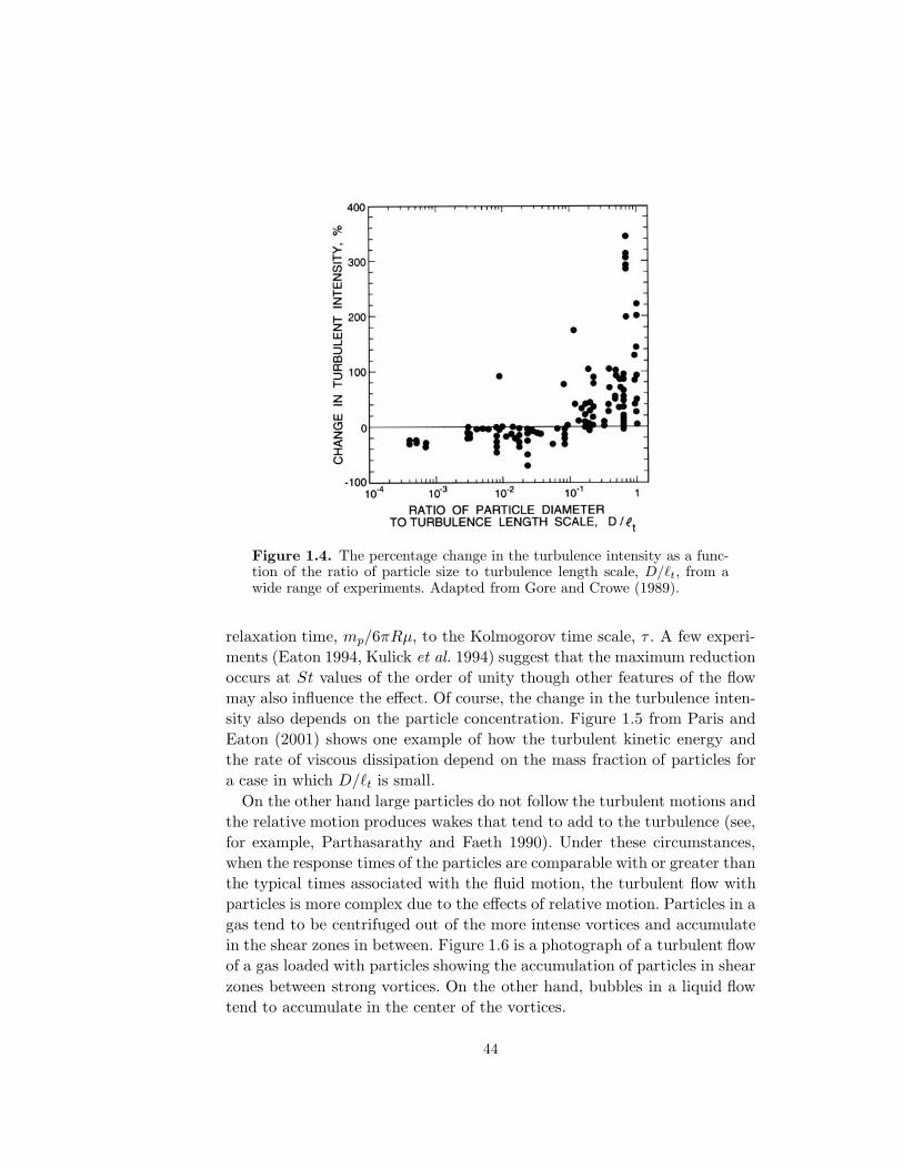
Figure 1.4. The percentage change in the turbulence intensity as a func-tion of the ratio of particle size to turbulence length scale, D/�t, from awide range of experiments. Adapted from Gore and Crowe (1989).

relaxation time, mp/6πRμ, to the Kolmogorov time scale, τ . A few experi-ments (Eaton 1994, Kulick et al. 1994) suggest that the maximum reductionoccurs at St values of the order of unity though other features of the flowmay also influence the effect. Of course, the change in the turbulence inten-sity also depends on the particle concentration. Figure 1.5 from Paris andEaton (2001) shows one example of how the turbulent kinetic energy andthe rate of viscous dissipation depend on the mass fraction of particles fora case in which D/�t is small.

On the other hand large particles do not follow the turbulent motions andthe relative motion produces wakes that tend to add to the turbulence (see,for example, Parthasarathy and Faeth 1990). Under these circumstances,when the response times of the particles are comparable with or greater thanthe typical times associated with the fluid motion, the turbulent flow withparticles is more complex due to the effects of relative motion. Particles in agas tend to be centrifuged out of the more intense vortices and accumulatein the shear zones in between. Figure 1.6 is a photograph of a turbulent flowof a gas loaded with particles showing the accumulation of particles in shearzones between strong vortices. On the other hand, bubbles in a liquid flowtend to accumulate in the center of the vortices.

44

Figure 1.5. The percentage change in the turbulent kinetic energy and therate of viscous dissipation with mass fraction for a channel flow of 150μmglass spheres suspended in air (from Paris and Eaton 2001).

Figure 1.6. Image of the centerplane of a fully developed, turbulent chan-nel flow of air loaded with 28μm particles. The area is 50mm by 30mm.Reproduced from Fessler et al.(1994) with the authors’ permission.

Analyses of turbulent flows with particles or bubbles are currently thesubject of active research and many issues remain. The literature includes anumber of heuristic and approximate quantitative analyses of the enhance-ment of turbulence due to particle relative motion. Examples are the workof Yuan and Michaelides (1992) and of Kenning and Crowe (1997). Thelatter relate the percentage change in the turbulence intensity due to theparticle wakes; this yields a percentage change that is a function not only of

45

D/�t but also of the mean relative motion and the density ratio. They showqualitative agreement with some of the data included in figure 1.4.

An alternative to these heuristic methodologies is the use of direct nu-merical simulations (DNS) to examine the details of the interaction betweenthe turbulence and the particles or bubbles. Such simulations have beencarried out both for solid particles (for example, Squires and Eaton 1990,Elghobashi and Truesdell 1993) and for bubbles (for example, Pan and Ba-narejee 1997). Because each individual simulation is so time consuming andleads to complex consequences, it is not possible, as yet, to draw generalconclusions over a wide parameter range. However, the kinds of particlesegregation mentioned above are readily apparent in the simulations.

1.3.2 Effect on turbulence stability

The issue of whether particles promote or delay transition to turbulence issomewhat distinct from their effect on developed turbulent flows. Saffman(1962) investigated the effect of dust particles on the stability of parallelflows and showed theoretically that if the relaxation time of the particles,tu, is small compared with �/U , the characteristic time of the flow, thenthe dust destabilizes the flow. Conversely if tu � �/U the dust stabilizes theflow.

In a somewhat similar investigation of the effect of bubbles on the sta-bility of parallel liquid flows, d’Agostino et al. (1997) found that the effectdepends on the relative magnitude of the most unstable frequency, ωm, andthe natural frequency of the bubbles, ωn (see section 4.4.1). When the ratio,ωm/ωn � 1, the primary effect of the bubbles is to increase the effective com-pressibility of the fluid and since increased compressibility causes increasedstability, the bubbles are stabilizing. On the other hand, at or near reso-nance when ωm/ωn is of order unity, there are usually bands of frequenciesin which the flow is less stable and the bubbles are therefore destabilizing.

In summary, when the response times of the particles or bubbles (boththe relaxation time and the natural period of volume oscillation) are shortcompared with the typical times associated with the fluid motion, the par-ticles simply alter the effective properties of the fluid, its effective density,viscosity and compressibility. It follows that under these circumstances thestability is governed by the effective Reynolds number and effective Machnumber. Saffman considered dusty gases at low volume concentrations, α,and low Mach numbers; under those conditions the net effect of the dust is tochange the density by (1 + αρS/ρG) and the viscosity by (1 + 2.5α). The ef-

46

fective Reynolds number therefore varies like (1 + αρS/ρG)/(1 + 2.5α). SinceρS � ρG the effective Reynolds number is increased and the dust is there-fore destabilizing. In the case of d’Agostino et al. the primary effect of thebubbles (when ωm � ωn) is to change the compressibility of the mixture.Since such a change is stabilizing in single phase flow, the result is that thebubbles tend to stabilize the flow.

On the other hand when the response times are comparable with or greaterthan the typical times associated with the fluid motion, the particles willnot follow the motions of the continuous phase. The disturbances caused bythis relative motion will tend to generate unsteady motions and promoteinstability in the continuous phase.

1.4 COMMENTS ON THE EQUATIONS OF MOTION

In sections 1.2.2 through 1.2.8 we assembled the basic form for the equationsof motion for a multiphase flow that would be used in a two-fluid model.However, these only provide the initial framework for there are many ad-ditional complications that must be addressed. The relative importance ofthese complications vary greatly from one type of multiphase flow to another.Consequently the level of detail with which they must be addressed variesenormously. In this general introduction we can only indicate the varioustypes of complications that can arise.

1.4.1 Averaging

As discussed in section 1.2.1, when the ratio of the particle size, D, to thetypical dimension of the averaging volume (estimated as the typical length,ε, over which there is significant change in the averaged flow properties)becomes significant, several issues arise (see Hinze 1959, Vernier and Delhaye1968, Nigmatulin 1979, Reeks 1992). The reader is referred to Slattery (1972)or Crowe et al. (1997) for a systematic treatment of these issues; only asummary is presented here. Clearly an appropriate volume average of aproperty, QC , of the continuous phase is given by < QC > where

< QC >=1VC

∫VC

QCdV (1.79)

47

where VC denotes the volume of the continuous phase within the controlvolume, V . For present purposes, it is also convenient to define an average

QC =1V

∫VC

QCdV = αC < QC > (1.80)

over the whole of the control volume.Since the conservation equations discussed in the preceding sections con-

tain derivatives in space and time and since the leading order set of equa-tions we seek are versions in which all the terms are averaged over some localvolume, the equations contain averages of spatial gradients and time deriva-tives. For these terms to be evaluated they must be converted to derivativesof the volume averaged properties. Those relations take the form (Crowe etal. 1997):

∂QC

∂xi=∂QC

∂xi− 1V

∫SD

QCnidS (1.81)

where SD is the total surface area of the particles within the averagingvolume. With regard to the time derivatives, if the volume of the particlesis not changing with time then

∂QC

∂t=∂QC

∂t(1.82)

but if the location of a point on the surface of a particle relative to its centeris given by ri and if ri is changing with time (for example, growing bubbles)then

∂QC

∂t=∂QC

∂t+

1V

∫SD

QCDriDt

dS (1.83)

When the definitions 1.81 and 1.83 are employed in the development ofappropriate averaged conservation equations, the integrals over the surfaceof the disperse phase introduce additional terms that might not have beenanticipated (see Crowe et al. 1997 for specific forms of those equations). Hereit is of value to observe that the magnitude of the additional surface integralterm in equation 1.81 is of order (D/ε)2. Consequently these additional termsare small as long as D/ε is sufficiently small.

1.4.2 Averaging contributions to the mean motion

Thus far we have discussed only those additional terms introduced as a resultof the fact that the gradient of the average may differ from the average of the

48

gradient. Inspection of the form of the basic equations (for example the con-tinuity equation, 1.21 or the momentum equation 1.42) readily demonstratesthat additional averaging terms will be introduced because the average of aproduct is different from the product of averages. In single phase flows, theReynolds stress terms in the averaged equations of motion for turbulent flowsare a prime example of this phenomenon. We will use the name quadraticrectification terms to refer to the appearance in the averaged equations ofmotion of the mean of two fluctuating components of velocity and/or volumefraction. Multiphase flows will, of course, also exhibit conventional Reynoldsstress terms when they become turbulent (see section 1.3 for more on thecomplicated subject of turbulence in multiphase flows). But even multiphaseflows that are not turbulent in the strictest sense will exhibit variations inthe velocities due the flows around particles and these variations will yieldquadratic rectification terms. These must be recognized and modeled whenconsidering the effects of locally non-uniform and unsteady velocities on theequations of motion. Much more has to be learned of both the laminar andturbulent quadratic rectification terms before these can be confidently in-corporated in model equations for multiphase flow. Both experiments andcomputer simulation will be valuable in this regard.

One simpler example in which the fluctuations in velocity have been mea-sured and considered is the case of concentrated granular flows in which di-rect particle-particle interactions create particle velocity fluctuations. Theseparticle velocity fluctuations and the energy associated with them (the so-called granular temperature) have been studied both experimentally andcomputationally (see chapter 13) and their role in the effective continuumequations of motion is better understood than in more complex multiphaseflows.

With two interacting phases or components, the additional terms thatemerge from an averaging process can become extremely complex. In recentdecades a number of valiant efforts have been made to codify these issuesand establish at least the forms of the important terms that result from theseinteractions. For example, Wallis (1991) has devoted considerable effort toidentify the inertial coupling of spheres in inviscid, locally irrotational flow.Arnold, Drew and Lahey (1989) and Drew (1991) have focused on the ap-plication of cell methods (see section 2.4.3) to interacting multiphase flows.Both these authors as well as Sangani and Didwania (1993) and Zhang andProsperetti (1994) have attempted to include the fluctuating motions of theparticles (as in granular flows) in the construction of equations of motion forthe multiphase flow; Zhang and Prosperetti also provide a useful compar-

49

ative summary of these various averaging efforts. However, it is also clearthat these studies have some distance to go before they can be incorporatedinto any real multiphase flow prediction methodology.

1.4.3 Averaging in pipe flows

One specific example of a quadratic rectification term (in this case a dis-crepancy between the product of an average and the average of a product)is that recognized by Zuber and Findlay (1965). In order to account for thevariations in velocity and volume fraction over the cross-section of a pipein constructing the one-dimensional equations of pipe flow, they found itnecessary to introduce a distribution parameter, C0, defined by

C0 =αj

α j(1.84)

where the overbar now represents an average over the cross-section of thepipe. The importance of C0 is best demonstrated by observing that it followsfrom equations 1.16 that the cross-sectionally averaged volume fraction, αA,is now related to the volume fluxes, jA and jB, by

αA =1C0

jA

(jA + jB)(1.85)

Values of C0 of the order of 1.13 (Zuber and Findlay 1965) or 1.25 (Wallis1969) appear necessary to match the experimental observations.

1.4.4 Modeling with the combined phase equations

One of the simpler approaches is to begin by modeling the combined phaseequations 1.24, 1.46 and 1.67 and hence avoid having to codify the mass,force and energy interaction terms. By defining mixture properties such asthe density, ρ, and the total volumetric flux, ji, one can begin to constructequations of motion in terms of those properties. But none of the summa-tion terms (equivalent to various weighted averages) in the combined phaseequations can be written accurately in terms of these mixture properties.For example, the summations,∑

N

ρNαNuNi and∑N

ρNαNuNiuNk (1.86)

are not necessarily given with any accuracy by ρji and ρjijk. Indeed, thediscrepancies are additional rectification terms that would require modeling

50

in such an approach. Thus any effort to avoid addressing the mass, force andenergy interaction terms by focusing exclusively on the mixture equationsof motion immediately faces difficult modeling questions.

1.4.5 Mass, force and energy interaction terms

Most multiphase flow modeling efforts concentrate on the individual phaseequations of motion and must therefore face the issues associated with con-struction of IN , the mass interaction term, FNk, the force interaction term,and EN , the energy interaction term. These represent the core of the prob-lem in modeling multiphase flows and there exist no universally applicablemethodologies that are independent of the topology of the flow, the flowpattern. Indeed, efforts to find systems of model equations that would beapplicable to a range of flow patterns would seem fruitless. Therein lies themain problem for the user who may not be able to predict the flow patternand therefore has little hope of finding an accurate and reliable method topredict flow rates, pressure drops, temperatures and other flow properties.

The best that can be achieved with the present state of knowledge is to at-tempt to construct heuristic models for IN , FNk, and EN given a particularflow pattern. Substantial efforts have been made in this direction partic-ularly for dispersed flows; the reader is directed to the excellent reviewsby Hinze (1961), Drew (1983), Gidaspow (1994) and Crowe et al. (1998)among others. Both direct experimentation and computer simulation havebeen used to create data from which heuristic expressions for the interactionterms could be generated. Computer simulations are particularly useful notonly because high fidelity instrumentation for the desired experiments is of-ten very difficult to develop but also because one can selectively incorporatea range of different effects and thereby evaluate the importance of each.

It is important to recognize that there are several constraints to whichany mathematical model must adhere. Any violation of those constraints islikely to produce strange and physically inappropriate results (see Garabe-dian 1964). Thus, the system of equations must have appropriate frame-indifference properties (see, for example, Ryskin and Rallison 1980). It mustalso have real characteristics; Prosperetti and Jones (1987) show that somemodels appearing in the literature do have real characteristics while othersdo not.

In this book chapters 2, 3 and 4 review what is known of the behavior ofindividual particles, bubbles and drops, with a view to using this informationto construct IN , FNk, and EN and therefore the equations of motion forparticular forms of multiphase flow.

51