Introduction to Cosmology - MSUalpha.sinp.msu.ru/.../roos_m_introduction_to_cosmology.pdf1.1...
299
Transcript of Introduction to Cosmology - MSUalpha.sinp.msu.ru/.../roos_m_introduction_to_cosmology.pdf1.1...


Introductionto Cosmology
Fourth Edition


Introductionto Cosmology
Fourth Edition
Matts Roos

This edition first published 2015© 2015 John Wiley & Sons, Ltd
Registered officeJohn Wiley & Sons Ltd, The Atrium, Southern Gate, Chichester, West Sussex, PO19 8SQ, UnitedKingdom
For details of our global editorial offices, for customer services and for information about how to applyfor permission to reuse the copyright material in this book please see our website at www.wiley.com.
The right of the author to be identified as the author of this work has been asserted in accordance withthe Copyright, Designs and Patents Act 1988.
All rights reserved. No part of this publication may be reproduced, stored in a retrieval system, ortransmitted, in any form or by any means, electronic, mechanical, photocopying, recording orotherwise, except as permitted by the UK Copyright, Designs and Patents Act 1988, without the priorpermission of the publisher.
Wiley also publishes its books in a variety of electronic formats. Some content that appears in print maynot be available in electronic books.
Designations used by companies to distinguish their products are often claimed as trademarks. Allbrand names and product names used in this book are trade names, service marks, trademarks orregistered trademarks of their respective owners. The publisher is not associated with any product orvendor mentioned in this book.
Limit of Liability/Disclaimer of Warranty: While the publisher and author have used their best efforts inpreparing this book, they make no representations or warranties with respect to the accuracy orcompleteness of the contents of this book and specifically disclaim any implied warranties ofmerchantability or fitness for a particular purpose. It is sold on the understanding that the publisher isnot engaged in rendering professional services and neither the publisher nor the author shall be liablefor damages arising herefrom. If professional advice or other expert assistance is required, the servicesof a competent professional should be sought
Library of Congress Cataloging-in-Publication Data applied for.
A catalogue record for this book is available from the British Library.
ISBN 978-1-118-92332-0 (paperback)
Set in 9.5/12.5pt, NewAsterLTStd by Laserwords Private Limited, Chennai, India
1 2015

To my family


Contents
Preface to First Edition xi
Preface to Second Edition xiii
Preface to Third Edition xv
Preface to Fourth Edition xvii
1 From Newton to Hubble 1
1.1 Historical Cosmology 21.2 Inertial Frames and the Cosmological Principle 61.3 Olbers’ Paradox 81.4 Hubble’s Law 111.5 The Age of the Universe 141.6 Matter in the Universe 161.7 Expansion in a Newtonian World 19
2 Special Relativity 25
2.1 Lorentz Transformations 252.2 Metrics of Curved Space-time 302.3 Relativistic Distance Measures 372.4 Tests of Special Relativity 45
3 General Relativity 49
3.1 The Principle of Equivalence 503.2 The Principle of Covariance 543.3 The Einstein Equation 583.4 Weak Field Limit 61

viii Contents
4 Tests of General Relativity 65
4.1 The Classical Tests 654.2 Binary Pulsars 674.3 Gravitational Lensing 694.4 Gravitational Waves 74
5 Cosmological Models 81
5.1 Friedmann–Lemaitre Cosmologies 815.2 de Sitter Cosmology 935.3 The Schwarzschild Model 955.4 Black Holes 965.5 Extended Gravity Models 106
6 Thermal History of the Universe 111
6.1 Planck Time 1126.2 The Primordial Hot Plasma 1126.3 Electroweak Interactions 1216.4 Photon and Lepton Decoupling 1286.5 Big Bang Nucleosynthesis 1346.6 Baryosynthesis and Antimatter Generation 142
7 Cosmic Inflation 151
7.1 Paradoxes of the Expansion 1527.2 Consensus Inflation 1587.3 The Chaotic Model 1657.4 Predictions 1687.5 A Cyclic Universe 169
8 Cosmic Microwave Background 175
8.1 The CMB Temperature 1768.2 Temperature Anisotropies 1808.3 Polarization 1858.4 Model Testing and Parameter Estimation 189
9 Dark Matter 199
9.1 Virially Bound Systems 2009.2 Galaxies 2039.3 Clusters 2089.4 Merging Galaxy Clusters 2119.5 Dark Matter Candidates 2139.6 The Cold Dark Matter Paradigm 218
10 Cosmic Structures 223
10.1 Density Fluctuations 22310.2 Structure Formation 228

Contents ix
11 Dark Energy 235
11.1 The Cosmological Constant 23511.2 Single Field Models 23811.3 f (R) Models 24611.4 Extra Dimensions 248
12 Epilogue 255
Tables 257
Index 261


Preface to First Edition
A few decades ago, astronomy and particle physics started to merge in the commonfield of cosmology. The general public had always been more interested in the visi-ble objects of astronomy than in invisible atoms, and probably met cosmology firstin Steven Weinberg’s famous book The First Three Minutes. More recently StephenHawking’s A Brief History of Time has caused an avalanche of interest in this subject.
Although there are now many popular monographs on cosmology, there are so farno introductory textbooks at university undergraduate level. Chapters on cosmologycan be found in introductory books on relativity or astronomy, but they cover onlypart of the subject. One reason may be that cosmology is explicitly cross-disciplinary,and therefore it does not occupy a prominent position in either physics or astronomycurricula.
At the University of Helsinki I decided to try to take advantage of the great inter-est in cosmology among the younger students, offering them a one-semester courseabout one year before their specialization started. Hence I could not count on muchfamiliarity with quantum mechanics, general relativity, particle physics, astrophysicsor statistical mechanics. At this level, there are courses with the generic name of Struc-ture of Matter dealing with Lorentz transformations and the basic concepts of quan-tum mechanics. My course aimed at the same level. Its main constraint was that ithad to be taught as a one-semester course, so that it would be accepted in physics andastronomy curricula. The present book is based on that course, given three times tophysics and astronomy students in Helsinki.
Of course there already exist good books on cosmology. The reader will in fact findmany references to such books, which have been an invaluable source of informationto me. The problem is only that they address a postgraduate audience that intendsto specialize in cosmology research. My readers will have to turn to these books laterwhen they have mastered all the professional skills of physics and mathematics.
In this book I am not attempting to teach basic physics to astronomers. They willneed much more. I am trying to teach just enough physics to be able to explain the

xii Preface to First Edition
main ideas in cosmology without too much hand-waving. I have tried to avoid theother extreme, practised by some of my particle physics colleagues, of writing bookson cosmology with the obvious intent of making particle physicists out of every theo-retical astronomer.
I also do not attempt to teach basic astronomy to physicists. In contrast to astron-omy scholars, I think the main ideas in cosmology do not require very detailedknowledge of astrophysics or observational techniques. Whole books have been writ-ten on distance measurements and the value of the Hubble parameter, which stillremains imprecise to a factor of two. Physicists only need to know that quantitiesentering formulae are measurable—albeit incorporating factors ℎ to some power—sothat the laws can be discussed meaningfully. At undergraduate level, it is not evenusual to give the errors on measured values.
In most chapters there are subjects demanding such a mastery of theoreticalphysics or astrophysics that the explanations have to be qualitative and the derivationsmeagre, for instance in general relativity, spontaneous symmetry breaking, inflationand galaxy formation. This is unavoidable because it just reflects the level of under-graduates. My intention is to go just a few steps further in these matters than do thepopular monographs.
I am indebted in particular to two colleagues and friends who offered constructivecriticism and made useful suggestions. The particle physicist Professor Kari Enqvistof NORDITA, Copenhagen, my former student, has gone to the trouble of readingthe whole manuscript. The space astronomer Professor Stuart Bowyer of the Univer-sity of California, Berkeley, has passed several early mornings of jet lag in Laplandgoing through the astronomy-related sections. Anyway, he could not go out skiingthen because it was either a snow storm or −30 ∘C! Finally, the publisher provided mewith a very knowledgeable and thorough referee, an astrophysicist no doubt, whosecriticism of the chapter on galaxy formation was very valuable to me. For all remain-ing mistakes I take full responsibility. They may well have been introduced by meafterwards.
Thanks are also due to friends among the local experts: particle physicist Profes-sor Masud Chaichian and astronomer Professor Kalevi Mattila have helped me withdetails and have answered my questions on several occasions. I am also indebted toseveral people who helped me to assemble the pictorial material: Drs Subir Sarkarin Oxford, Rocky Kolb in the Fermilab, Carlos Frenk in Durham, Werner Kienzle atCERN and members of the COBE team.
Finally, I must thank my wife Jacqueline for putting up with almost two years ofnear absence and full absent-mindedness while writing this book.
Matts Roos

Preface to Second Edition
In the three years since the first edition of this book was finalized, the field of cos-mology has seen many important developments, mainly due to new observations withsuperior instruments such as the Hubble Space Telescope and the ground-based Kecktelescope and many others. Thus a second edition has become necessary in order toprovide students and other readers with a useful and up to date textbook and refer-ence book.
At the same time I could balance the presentation with material which was notadequately covered before—there I am in debt to many readers. Also, the inevitablenumber of misprints, errors and unclear formulations, typical of a first edition, couldbe corrected. I am especially indebted to Kimmo Kainulainen who served as my courseassistant one semester, and who worked through the book and the problems thor-oughly, resulting in a very long list of corrigenda. A similar shorter list was also dressedby George Smoot and a student of his. It still worries me that the errors found byGeorge had been found neither by Kimmo nor by myself, thus statistics tells me thatsome errors still will remain undetected.
For new pictorial material I am indebted to Wes Colley at Princeton, Carlos Frenkin Durham, Charles Lineweaver in Strasbourg, Jukka Nevalainen in Helsinki, SubirSarkar in Oxford, and George Smoot in Berkeley. I am thankful to the Academie desSciences for an invitation to Paris where I could visit the Observatory of Paris-Meudonand profit from discussions with S. Bonazzola and Brandon Carter.
Several of my students have contributed in various ways: by misunderstandings,indicating the need for better explanations, by their enthusiasm for the subject, and bytechnical help, in particular S. M. Harun-or-Rashid. My youngest grandchild Adrian(not yet 3) has showed a vivid interest for supernova bangs, as demonstrated by anX-ray image of the Cassiopeia A remnant. Thus the future of the subject is bright.
Matts Roos


Preface to Third Edition
This preface can start just like the previous one: in the seven years since the secondedition was finalized, the field of cosmology has seen many important developments,mainly due to new observations with superior instruments. In the past, cosmologyoften relied on philosophical or aesthetic arguments; now it is maturing to becomean exact science. For example, the Einstein–de Sitter universe, which has zero cos-mological constant (𝛺
𝜆= 0), used to be favored for esthetical reasons, but today it is
known to be very different from zero (𝛺𝜆= 0.73 ± 0.04).
In the first edition I quoted𝛺0 = 0.8 ± 0.3 (daring to believe in errors that many oth-ers did not), which gave room for all possible spatial geometries: spherical, flat andhyperbolic. Since then the value has converged to 𝛺0 = 1.02 ± 0.02, and everybody isnow willing to concede that the geometry of the Universe is flat, 𝛺0 = 1. This resultis one of the cornerstones of what we now can call the ‘Concordance Model of Cos-mology’. Still, deep problems remain, so deep that even Einstein’s general relativity isoccasionally put in doubt.
A consequence of the successful march towards a ‘concordance model’ is that manyalternative models can be discarded. An introductory text of limited length like the cur-rent one cannot be a historical record of failed models. Thus I no longer discuss, ordiscuss only briefly, 𝑘 ≠ 0 geometries, the Einstein–de Sitter universe, hot and warmdark matter, cold dark matter models with 𝜆 = 0, isocurvature fluctuations, topologi-cal defects (except monopoles), Bianchi universes, and formulae which only work indiscarded or idealized models, like Mattig’s relation and the Saha equation.
Instead, this edition contains many new or considerably expanded subjects:Section 2.3 on Relativistic Distance Measures, Section 3.3 on GravitationalLensing, Section 3.5 on Gravitational Waves, Section 4.3 on Dark Energy andQuintessence, Section 5.1 on Photon Polarization, Section 7.4 on The Inflatonas Quintessence, Section 7.5 on Cyclic Models, Section 8.3 on CMB PolarizationAnisotropies, Section 8.4 on model testing and parameter estimation using mainly thefirst-year CMB results of the Wilkinson Microwave Anisotropy Probe, and Section 9.5

xvi Preface to Third Edition
on large-scale structure results from the 2 degree Field (2dF) Galaxy Redshift Survey.The synopsis in this edition is also different and hopefully more logical, much hasbeen entirely rewritten, and all parameter values have been updated.
I have not wanted to go into pure astrophysics, but the line between cosmologyand cosmologically important astrophysics is not easy to draw. Supernova explo-sion mechanisms and black holes are included as in the earlier editions, but notfor instance active galactic nuclei (AGNs) or jets or ultra-high-energy cosmic rays.Observational techniques are mentioned only briefly—they are beyond the scope ofthis book.
There are many new figures for which I am in debt to colleagues and friends, allacknowledged in the figure legends. I have profited from discussions with ProfessorCarlos Frenk at the University of Durham and Professor Kari Enqvist at the Universityof Helsinki. I am also indebted to Professor Juhani Keinonen at the University ofHelsinki for having generously provided me with working space and access to all thefacilities at the Department of Physical Sciences, despite the fact that I am retired.
Many critics, referees and other readers have made useful comments that I havetried to take into account. One careful reader, Urbana Lopes França Jr, sent me a longlist of misprints and errors. A critic of the second edition stated that the errors in thefirst edition had been corrected, but that new errors had emerged in the new text. Thiswill unfortunately always be true in any comparison of edition 𝑛 + 1 with edition 𝑛.In an attempt to make continuous corrections I have assigned a web site for a list oferrors and misprints.
My most valuable collaborator has been Thomas S. Coleman, a nonphysicistwho contacted me after having spotted some errors in the second edition, and whoproposed some improvements in case I were writing a third edition. This cameat the appropriate time and led to a collaboration in which Thomas S. Colemanread the whole manuscript, corrected misprints, improved my English, checked mycalculations, designed new figures and proposed clarifications where he found thetext difficult.
My wife Jacqueline has many interesting subjects of conversation at the break-fast table. Regretfully, her breakfast companion is absent-minded, thinking only ofcosmology. I thank her heartily for her kind patience, promising improvement.
Matts Roos

Preface to Fourth Edition
Just like the previous times I can state that the field of cosmology has seen so manyimportant developments in the 11 years since the third edition that a fourth editionhas become necessary.
In the first Chapter there is a new section presenting briefly various forms of bary-onic matter: in supernovae and neutron stars and in noncollapsed objects such asinterstellar dust, hot gas in the intergalactic medium, the cosmic rays, neutrinos andantiparticles. Active galactic nuclei, gamma ray bursts and quasars are also men-tioned. The Hubble parameter and the age of the Universe are updated.
Chapter 2 is reorganized to contain only special relativity whereas all of generalrelativity forms Chapter 3. Chapter 2 ends with a brief new section on tests of specialrelativity and variable speed of light.
In the previous editions the Einstein equation was “derived” in the weak field limitwith some hand-waving arguments. That derivation is still in Chapter 3, but the Ein-stein equation is now properly derived from the Hilbert–Einstein action. To somereaders the derivation will then be more difficult, but one can of course skip it and besatisfied with the weak field limit. How to incorporate the energy of a gravitationalfield as a pseudotensor is briefly mentioned.
Chapter 4 addresses tests of general relativity with the exception for black holeswhich are now in Chapter 5. A new binary pulsar has been added and the section ondetectors of gravitational radiation has been updated.
Chapter 5 on cosmological models contains the Schwarzschild model (previouslyin Chapter 2), a considerably expanded and modernized section on black holes, some-what speculative perhaps, because it is based on Hawking’s recent ideas. The lastsection is entirely new, it discusses extended gravity models starting from a gener-alization of the Einstein–Hilbert action, and it lays the basis for dark energy modelsin Chapter 11.
Chapter 6 is now a very much abridged version of the previous chapters 5 on thethermal history of the Universe and 6 on particles and symmetries. This reduction was
xviii Preface to Fourth Edition
necessary in order to make space for all the new matter. What has disappeared wasstandard particle physics which should be known to the particle physics readership(the astronomers do not care).
In Chapter 7 on inflation the currently popular single-field model is rewritten andmuch expanded.
In Chapter 8 on the cosmic microwave background the emphasis has been shiftedfrom the WMAP satellite to Planck, and all the parameter values have been updated.
Dark matter has been dedicated its own Chapter 9, very much enlarged from thematerial in the previous edition, and concentrated on the abundant observations ofits gravitational effects. Very little is said about dark matter candidates since that isall speculative.
In the very short Chapter 10 on cosmic structures there is nothing new added.Finally Chapter 11 is devoted to dark energy, almost entirely new in this edition.I have enjoyed the support of the Magnus Ehrnrooth Foundation for the work on
this Edition.
Matts RoosHelsinki, May 2014

1
From Newton toHubble
The history of ideas on the structure and origin of the Universe shows that humankindhas always put itself at the center of creation. As astronomical evidence has accumu-lated, these anthropocentric convictions have had to be abandoned one by one. Fromthe natural idea that the solid Earth is at rest and the celestial objects all rotate aroundus, we have come to understand that we inhabit an average-sized planet orbiting anaverage-sized sun, that the Solar System is in the periphery of a rotating galaxy ofaverage size, flying at hundreds of kilometres per second towards an unknown goalin an immense Universe, containing billions of similar galaxies.
Cosmology aims to explain the origin and evolution of the entire contents of theUniverse, the underlying physical processes, and thereby to obtain a deeper under-standing of the laws of physics assumed to hold throughout the Universe. Unfortu-nately, we have only one universe to study, the one we live in, and we cannot makeexperiments with it, only observations. This puts serious limits on what we can learnabout the origin. If there are other universes we will never know.
Although the history of cosmology is long and fascinating, we shall not trace it indetail, nor any further back than Newton, accounting (in Section 1.1) only for thoseideas which have fertilized modern cosmology directly, or which happened to be rightalthough they failed to earn timely recognition. In the early days of cosmology, whenlittle was known about the Universe, the field was really just a branch of philosophy.
Having a rigid Earth to stand on is a very valuable asset. How can we describemotion except in relation to a fixed point? Important understanding has come fromthe study of inertial systems, in uniform motion with respect to one another. Fromthe work of Einstein on inertial systems, the theory of special relativity was born. InSection 1.2 we discuss inertial frames, and see how expansion and contraction arenatural consequences of the homogeneity and isotropy of the Universe.
Introduction to Cosmology, Fourth Edition. Matts Roos© 2015 John Wiley & Sons, Ltd. Published 2015 by John Wiley & Sons, Ltd.

2 From Newton to Hubble
A classic problem is why the night sky is dark and not blazing like the disc of theSun, as simple theory in the past would have it. In Section 1.3 we shall discuss thisso-called Olbers’ paradox, and the modern understanding of it.
The beginning of modern cosmology may be fixed at the publication in 1929 of Hub-ble’s law, which was based on observations of the redshift of spectral lines from remotegalaxies. This was subsequently interpreted as evidence for the expansion of the Uni-verse, thus ruling out a static Universe and thereby setting the primary requirementon theory. This will be explained in Section 1.4. In Section 1.5 we turn to determina-tions of cosmic timescales and the implications of Hubble’s law for our knowledge ofthe age of the Universe.
In Section 1.6 we describe Newton’s theory of gravitation, which is the earliestexplanation of a gravitational force. We shall ‘modernize’ it by introducing Hubble’slaw into it. In fact, we shall see that this leads to a cosmology which already containsmany features of current Big Bang cosmologies.
1.1 Historical Cosmology
At the time of Isaac Newton (1642–1727) the heliocentric Universe of Nicolaus Coper-nicus (1473–1543), Galileo Galilei (1564–1642) and Johannes Kepler (1571–1630) hadbeen accepted, because no sensible description of the motion of the planets could befound if the Earth was at rest at the center of the Solar System. Humankind was thusdethroned to live on an average-sized planet orbiting around an average-sized sun.
The stars were understood to be suns like ours with fixed positions in a static Uni-verse. The Milky Way had been resolved into an accumulation of faint stars with thetelescope of Galileo. The anthropocentric view still persisted, however, in locating theSolar System at the center of the Universe.
Newton’s Cosmology. The first theory of gravitation appeared when Newton pub-lished his Philosophiae Naturalis Principia Mathematica in 1687. With this theory hecould explain the empirical laws of Kepler: that the planets moved in elliptical orbitswith the Sun at one of the focal points. An early success of this theory came whenEdmund Halley (1656–1742) successfully predicted that the comet sighted in 1456,1531, 1607 and 1682 would return in 1758. Actually, the first observation confirmingthe heliocentric theory came in 1727 when James Bradley (1693–1762) discovered theaberration of starlight, and explained it as due to the changes in the velocity of theEarth in its annual orbit. In our time, Newton’s theory of gravitation still suffices todescribe most of planetary and satellite mechanics, and it constitutes the nonrelativis-tic limit of Einstein’s relativistic theory of gravitation.
Newton considered the stars to be suns evenly distributed throughout infinitespace in spite of the obvious concentration of stars in the Milky Way. A distribution iscalled homogeneous if it is uniformly distributed, and it is called isotropic if it has thesame properties in all spatial directions. Thus in a homogeneous and isotropic spacethe distribution of matter would look the same to observers located anywhere—nopoint would be preferential. Each local region of an isotropic universe contains

Historical Cosmology 3
information which remains true also on a global scale. Clearly, matter introduceslumpiness which grossly violates homogeneity on the scale of stars, but on somelarger scale isotropy and homogeneity may still be a good approximation. Goingone step further, one may postulate what is called the cosmological principle, orsometimes the Copernican principle.
The Universe is homogeneous and isotropic in three-dimensional space, hasalways been so, and will always remain so.
It has always been debated whether this principle is true, and on what scale. On thegalactic scale visible matter is lumpy, and on larger scales galaxies form gravitation-ally bound clusters and narrow strings separated by voids. But galaxies also appear toform loose groups of three to five or more galaxies. Several surveys have now reachedagreement that the distribution of these galaxy groups appears to be homogeneousand isotropic within a sphere of 170 Mpc radius [1]. This is an order of magnitudelarger than the supercluster to which our Galaxy and our local galaxy group or LocalSupercluster (LSC) belong, and which is centered in the constellation of Virgo. Basedon his theory of gravitation, Newton formulated a cosmology in 1691. Since all mas-sive bodies attract each other, a finite system of stars distributed over a finite regionof space should collapse under their mutual attraction. But this was not observed,in fact the stars were known to have had fixed positions since antiquity, and Newtonsought a reason for this stability. He concluded, erroneously, that the self-gravitationwithin a finite system of stars would be compensated for by the attraction of a suffi-cient number of stars outside the system, distributed evenly throughout infinite space.However, the total number of stars could not be infinite because then their attractionwould also be infinite, making the static Universe unstable. It was understood onlymuch later that the addition of external layers of stars would have no influence on thedynamics of the interior. The right conclusion is that the Universe cannot be static,an idea which would have been too revolutionary at the time.
Newton’s contemporary and competitor Gottfried Wilhelm von Leibnitz (1646–1716)also regarded the Universe to be spanned by an abstract infinite space, but in contrastto Newton he maintained that the stars must be infinite in number and distributed allover space, otherwise the Universe would be bounded and have a center, contrary tocontemporary philosophy. Finiteness was considered equivalent to boundedness, andinfinity to unboundedness.
Rotating Galaxies. The first description of the Milky Way as a rotating galaxy can betraced to Thomas Wright (1711–1786), who wrote An Original Theory or New Hypoth-esis of the Universe in 1750, suggesting that the stars are
all moving the same way and not much deviating from the same plane, as theplanets in their heliocentric motion do round the solar body.
Wright’s galactic picture had a direct impact on Immanuel Kant (1724–1804).In 1755 Kant went a step further, suggesting that the diffuse nebulae whichGalileo had already observed could be distant galaxies rather than nearby clouds of

4 From Newton to Hubble
incandescent gas. This implied that the Universe could be homogeneous on the scaleof galactic distances in support of the cosmological principle.
Kant also pondered over the reason for transversal velocities such as the movementof the Moon. If the Milky Way was the outcome of a gaseous nebula contracting underNewton’s law of gravitation, why was all movement not directed towards a commoncenter? Perhaps there also existed repulsive forces of gravitation which would scat-ter bodies onto trajectories other than radial ones, and perhaps such forces at largedistances would compensate for the infinite attraction of an infinite number of stars?Note that the idea of a contracting gaseous nebula constituted the first example of anonstatic system of stars, but at galactic scale with the Universe still static.
Kant thought that he had settled the argument between Newton and Leibnitz aboutthe finiteness or infiniteness of the system of stars. He claimed that either type ofsystem embedded in an infinite space could not be stable and homogeneous, and thusthe question of infinity was irrelevant. Similar thoughts can be traced to the scholarYang Shen in China at about the same time, then unknown to Western civilization [2].
The infinity argument was, however, not properly understood until Bernhard Rie-mann (1826–1866) pointed out that the world could be finite yet unbounded, providedthe geometry of the space had a positive curvature, however small. On the basis ofRiemann’s geometry, Albert Einstein (1879–1955) subsequently established the con-nection between the geometry of space and the distribution of matter.
Kant’s repulsive force would have produced trajectories in random directions, butall the planets and satellites in the Solar System exhibit transversal motion in one andthe same direction. This was noticed by Pierre Simon de Laplace (1749–1827), whorefuted Kant’s hypothesis by a simple probabilistic argument in 1825: the observedmovements were just too improbable if they were due to random scattering by arepulsive force. Laplace also showed that the large transversal velocities and theirdirection had their origin in the rotation of the primordial gaseous nebula and the lawof conservation of angular momentum. Thus no repulsive force is needed to explainthe transversal motion of the planets and their moons, no nebula could contract to apoint, and the Moon would not be expected to fall down upon us.
This leads to the question of the origin of time: what was the first cause of therotation of the nebula and when did it all start? This is the question modern cosmologyattempts to answer by tracing the evolution of the Universe backwards in time andby reintroducing the idea of a repulsive force in the form of a cosmological constantneeded for other purposes.
Black Holes. The implications of Newton’s gravity were quite well understood byJohn Michell (1724–1793), who pointed out in 1783 that a sufficiently massive andcompact star would have such a strong gravitational field that nothing could escapefrom its surface. Combining the corpuscular theory of light with Newton’s theory, hefound that a star with the solar density and escape velocity 𝑐 would have a radius of486𝑅
⊙and a mass of 120 million solar masses. This was the first mention of a type
of star much later to be called a black hole (to be discussed in Section 3.4). In 1796Laplace independently presented the same idea.

Historical Cosmology 5
Galactic and Extragalactic Astronomy. Newton should also be credited with theinvention of the reflecting telescope—he even built one—but the first one ofimportance was built one century later by William Herschel (1738–1822). With thisinstrument, observational astronomy took a big leap forward: Herschel and his sonJohn could map the nearby stars well enough in 1785 to conclude correctly that theMilky Way was a disc-shaped star system. They also concluded erroneously that theSolar System was at its center, but many more observations were needed before itwas corrected. Herschel made many important discoveries, among them the planetUranus, and some 700 binary stars whose movements confirmed the validity of New-ton’s theory of gravitation outside the Solar System. He also observed some 250 diffusenebulae, which he first believed were distant galaxies, but which he and many otherastronomers later considered to be nearby incandescent gaseous clouds belonging toour Galaxy. The main problem was then to explain why they avoided the directions ofthe galactic disc, since they were evenly distributed in all other directions.
The view of Kant that the nebulae were distant galaxies was also defended byJohann Heinrich Lambert (1728–1777). He came to the conclusion that the Solar Sys-tem along, with the other stars in our Galaxy, orbited around the galactic center, thusdeparting from the heliocentric view. The correct reason for the absence of nebulaein the galactic plane was only given by Richard Anthony Proctor (1837–1888), whoproposed the presence of interstellar dust. The arguments for or against the interpre-tation of nebulae as distant galaxies nevertheless raged throughout the 19th centurybecause it was not understood how stars in galaxies more luminous than the wholegalaxy could exist—these were observations of supernovae. Only in 1925 did EdwinP. Hubble (1889–1953) resolve the conflict indisputably by discovering Cepheids andordinary stars in nebulae, and by determining the distance to several galaxies, amongthem the celebrated M31 galaxy in the Andromeda. Although this distance was off bya factor of two, the conclusion was qualitatively correct.
In spite of the work of Kant and Lambert, the heliocentric picture of the Galaxy—oralmost heliocentric since the Sun was located quite close to Herschel’s galacticcenter—remained long into our century. A decisive change came with the observationsin 1915–1919 by Harlow Shapley (1895–1972) of the distribution of globular clustershosting 105–107 stars. He found that perpendicular to the galactic plane they were uni-formly distributed, but along the plane these clusters had a distribution which peakedin the direction of the Sagittarius. This defined the center of the Galaxy to be quite farfrom the Solar System: we are at a distance of about two-thirds of the galactic radius.Thus the anthropocentric world picture received its second blow—and not the lastone—if we count Copernicus’s heliocentric picture as the first one. Note that Shapleystill believed our Galaxy to be at the center of the astronomical Universe.
The End of Newtonian Cosmology. In 1883 Ernst Mach (1838–1916) publisheda historical and critical analysis of mechanics in which he rejected Newton’s con-cept of an absolute space, precisely because it was unobservable. Mach demandedthat the laws of physics should be based only on concepts which could be related toobservations. Since motion still had to be referred to some frame at rest, he proposedreplacing absolute space by an idealized rigid frame of fixed stars. Thus ‘uniform

6 From Newton to Hubble
motion’ was to be understood as motion relative to the whole Universe. AlthoughMach clearly realized that all motion is relative, it was left to Einstein to take the fullstep of studying the laws of physics as seen by observers in inertial frames in relativemotion with respect to each other.
Einstein published his General Theory of Relativity in 1917, but the only solution hefound to the highly nonlinear differential equations was that of a static Universe. Thiswas not so unsatisfactory though, because the then known Universe comprised onlythe stars in our Galaxy, which indeed was seen as static, and some nebulae of ill-knowndistance and controversial nature. Einstein firmly believed in a static Universe until hemet Hubble in 1929 and was overwhelmed by the evidence for what was to be calledHubble’s law.
Immediately after general relativity became known, Willem de Sitter (1872–1934)published (in 1917) another solution, for the case of empty space-time in an expo-nential state of expansion. In 1922 the Russian meteorologist Alexandr Friedmann(1888–1925) found a range of intermediate solutions to the Einstein equation whichdescribe the standard cosmology today. Curiously, this work was ignored for a decadealthough it was published in widely read journals.
In 1924 Hubble had measured the distances to nine spiral galaxies, and he foundthat they were extremely far away. The nearest one, M31 in the Andromeda, is nowknown to be at a distance of 20 galactic diameters (Hubble’s value was about 8) andthe farther ones at hundreds of galactic diameters. These observations established thatthe spiral nebulae are, as Kant had conjectured, stellar systems comparable in massand size with the Milky Way, and their spatial distribution confirmed the expectationsof the cosmological principle on the scale of galactic distances.
In 1926–1927 Bertil Lindblad (1895–1965) and Jan Hendrik Oort (1900–1992) ver-ified Laplace’s hypothesis that the Galaxy indeed rotated, and they determined theperiod to be 108 yr and the mass to be about 1011𝑀
⊙. The conclusive demonstration
that the Milky Way is an average-sized galaxy, in no way exceptional or central, wasgiven only in 1952 by Walter Baade. This we may count as the third breakdown of theanthropocentric world picture.
The later history of cosmology up until 1990 has been excellently summarized byPeebles [3].
To give the reader an idea of where in the Universe we are, what is nearby andwhat is far away, some cosmic distances are listed in Table A.1 in the appendix. Ona cosmological scale we are not really interested in objects smaller than a galaxy!We generally measure cosmic distances in parsec (pc) units (kpc for 103 pc and Mpcfor 106 pc). A parsec is the distance at which one second of arc is subtended by alength equalling the mean distance between the Sun and the Earth. The parsec unit isgiven in Table A.2 in the appendix, where the values of some useful cosmological andastrophysical constants are listed.
1.2 Inertial Frames and the Cosmological Principle
Newton’s first law—the law of inertia—states that a system on which no forcesact is either at rest or in uniform motion. Such systems are called inertial frames.

Inertial Frames and the Cosmological Principle 7
Accelerated or rotating frames are not inertial frames. Newton considered that ‘atrest’ and ‘in motion’ implicitly referred to an absolute space which was unobservablebut which had a real existence independent of humankind. Mach rejected the notionof an empty, unobservable space, and only Einstein was able to clarify the physics ofmotion of observers in inertial frames.
It may be interesting to follow a nonrelativistic argument about the static ornonstatic nature of the Universe which is a direct consequence of the cosmologicalprinciple.
Consider an observer ‘A’ in an inertial frame who measures the density of galaxiesand their velocities in the space around him. Because the distribution of galaxies isobserved to be homogeneous and isotropic on very large scales (strictly speaking, thisis actually true for galaxy groups [1]), he would see the same mean density of galaxies(at one time 𝑡) in two different directions r and r′:
𝜌A(r, 𝑡) = 𝜌A(r′, 𝑡).
Another observer ‘B’ in another inertial frame (see Figure 1.1) looking in the directionr from her location would also see the same mean density of galaxies:
𝜌B(r′, 𝑡) = 𝜌A(r, 𝑡).
The velocity distributions of galaxies would also look the same to both observers, infact in all directions, for instance in the r′ direction:
𝒗B(r′, 𝑡) = 𝒗A(r′, 𝑡).
Suppose that the B frame has the relative velocity 𝒗A (r′′, 𝑡) as seen from the A framealong the radius vector r′′ = r − r′. If all velocities are nonrelativistic, i.e. small com-pared with the speed of light, we can write
𝒗A(r′, 𝑡) = 𝒗A(r − r′′, 𝑡) = 𝒗A(r, 𝑡) − 𝒗A(r′′, 𝑡).
This equation is true only if 𝒗A (r, 𝑡) has a specific form: it must be proportional to r,
𝒗A(r, 𝑡) = 𝑓 (𝑡)r, (1.1)
where 𝑓 (𝑡) is an arbitrary function. Why is this so?Let this universe start to expand. From the vantage point of A (or B equally well,
since all points of observation are equal), nearby galaxies will appear to recede slowly.
A
r'
r'
d
r
B
P
Figure 1.1 Two observers at A and B making observations in the directions r, r′.
8 From Newton to Hubble
But in order to preserve uniformity, distant ones must recede faster, in fact theirrecession velocities must increase linearly with distance. That is the content of Equa-tion (1.1).
If 𝑓 (𝑡) > 0, the Universe would be seen by both observers to expand, each galaxyhaving a radial velocity proportional to its radial distance r. If 𝑓 (𝑡) < 0, the Universewould be seen to contract with velocities in the reversed direction. Thus we have seenthat expansion and contraction are natural consequences of the cosmological princi-ple. If 𝑓 (𝑡) is a positive constant, Equation (1.1) is Hubble’s law.
Actually, it is somewhat misleading to say that the galaxies recede when, rather, it isspace itself which expands or contracts. This distinction is important when we cometo general relativity.
A useful lesson may be learned from studying the limited gravitational system con-sisting of the Earth and rockets launched into space. This system is not quite like theprevious example because it is not homogeneous, and because the motion of a rocketor a satellite in Earth’s gravitational field is different from the motion of galaxies in thegravitational field of the Universe. Thus to simplify the case we only consider radialvelocities, and we ignore Earth’s rotation. Suppose the rockets have initial velocitieslow enough to make them fall back onto Earth. The rocket–Earth gravitational systemis then closed and contracting, corresponding to 𝑓 (𝑡) < 0.
When the kinetic energy is large enough to balance gravity, our idealized rocketbecomes a satellite, staying above Earth at a fixed height (real satellites circulate instable Keplerian orbits at various altitudes if their launch velocities are in the range8–11 km s−1). This corresponds to the static solution 𝑓 (𝑡) = 0 for the rocket–Earth grav-itational system.
If the launch velocities are increased beyond about 11 km s−1, the potential energyof Earth’s gravitational field no longer suffices to keep the rockets bound to Earth.Beyond this speed, called the second cosmic velocity by rocket engineers, the rocketsescape for good. This is an expanding or open gravitational system, corresponding to𝑓 (𝑡) > 0.
The static case is different if we consider the Universe as a whole. According tothe cosmological principle, no point is preferred, and therefore there exists no centeraround which bodies can gravitate in steady-state orbits. Thus the Universe is eitherexpanding or contracting, the static solution being unstable and therefore unlikely.
1.3 Olbers’ Paradox
Let us turn to an early problem still discussed today, which is associated with thename of Wilhelm Olbers (1758–1840), although it seems to have been known alreadyto Kepler in the 17th century, and a treatise on it was published by Jean-Philippe Loysde Chéseaux in 1744, as related in the book by E. Harrison [4]. Why is the night skydark if the Universe is infinite, static and uniformly filled with stars? They should fillup the total field of visibility so that the night sky would be as bright as the Sun, andwe would find ourselves in the middle of a heat bath of the temperature of the surface

Olbers’ Paradox 9
of the Sun. Obviously, at least one of the above assumptions about the Universe mustbe wrong.
The question of the total number of shining stars was already pondered by Newtonand Leibnitz. Let us follow in some detail the argument published by Olbers in 1823.The absolute luminosity of a star is defined as the amount of luminous energy radiatedper unit time, and the surface brightness 𝐵 as luminosity per unit surface. Let theapparent luminosity of a star of absolute luminosity L at distance 𝑟 from an observerbe 𝑙 = 𝐿∕4𝜋𝑟2.
Suppose that the number of stars with average luminosity 𝐿 is𝑁 and their averagedensity in a volume 𝑉 is 𝑛 = 𝑁∕𝑉 . If the surface area of an average star is 𝐴, thenits brightness is 𝐵 = 𝐿∕𝐴. The Sun may be taken to be such an average star, mainlybecause we know it so well.
The number of stars in a spherical shell of radius 𝑟 and thickness d𝑟 is then 4𝜋𝑟2𝑛 d𝑟.Their total radiation as observed at the origin of a static universe of infinite extent isthen found by integrating the spherical shells from 0 to ∞:
∫
∞
04𝜋𝑟2nl d𝑟 =
∫
∞
0nL d𝑟 = ∞. (1.2)
On the other hand, a finite number of visible stars each taking up an angle 𝐴∕𝑟2 couldcover an infinite number of more distant stars, so it is not correct to integrate 𝑟 to ∞.Let us integrate only up to such a distance 𝑅 that the whole sky of angle 4𝜋 would beevenly tiled by the star discs. The condition for this is
∫
𝑅
04𝜋𝑟2𝑛 𝐴
𝑟2d𝑟 = 4𝜋.
It then follows that the distance is 𝑅 = 1∕An. The integrated brightness from thesevisible stars alone is then
∫
𝑅
0nL d𝑟 = 𝐿∕𝐴, (1.3)
or equal to the brightness of the Sun. But the night sky is indeed dark, so we are facedwith a paradox.
Olbers’ own explanation was that invisible interstellar dust absorbed the light. Thatwould make the intensity of starlight decrease exponentially with distance. But onecan show that the amount of dust needed would be so great that the Sun would alsobe obscured. Moreover, the radiation would heat the dust so that it would start to glowsoon enough, thereby becoming visible in the infrared.
A large number of different solutions to this paradox have been proposed in thepast, some of the wrong ones lingering on into the present day. Let us here follow avalid line of reasoning due to Lord Kelvin (1824–1907), as retold and improved in apopular book by E. Harrison [4].
A star at distance 𝑟 covers the fraction 𝐴∕4𝜋𝑟2 of the sky. Multiplying this by thenumber of stars in the shell, 4𝜋𝑟2𝑛 d𝑟, we obtain the fraction of the whole sky coveredby stars viewed by an observer at the center, An d𝑟. Since 𝑛 is the star count per

10 From Newton to Hubble
volume element, An has the dimensions of number of stars per linear distance. Theinverse of this,
𝓁 = 1∕An, (1.4)
is the mean radial distance between stars, or the mean free path of photons emittedfrom one star and being absorbed in collisions with another. We can also define amean collision time:
𝜏 = 𝓁∕𝑐. (1.5)
The value of 𝜏 can be roughly estimated from the properties of the Sun, with radius𝑅⊙
and density 𝜌⊙
. Let the present mean density of luminous matter in the Universebe 𝜌0 and the distance to the farthest visible star 𝑟∗. Then the collision time inside thisvolume of size 4
3𝜋𝑟3∗ is
𝜏 ≃ 𝜏⊙= 1𝐴⊙
nc= 1𝜋𝑅
2⊙
4𝜋𝑟3∗3Nc
=4𝜌
⊙𝑅⊙
3𝜌0𝑐. (1.6)
Taking the solar parameters from Table A.2 in the appendix we obtain approximately1023 yr.
The probability that a photon does not collide but arrives safely to be observed by usafter a flight distance 𝑟 can be derived from the assumption that the photon encountersobstacles randomly, that the collisions occur independently and at a constant rate 𝓁−1
per unit distance. The probability 𝑃 (𝑟) that the distance to the first collision is 𝑟 is thengiven by the exponential distribution
𝑃 (𝑟) = 𝓁−1e−𝑟∕𝓁 . (1.7)
Thus flight distances much longer than 𝓁 are improbable.Applying this to photons emitted in a spherical shell of thickness d𝑟, and integrating
the spherical shell from zero radius to 𝑟∗, the fraction of all photons emitted in thedirection of the center of the sphere and arriving there to be detected is
𝑓 (𝑟∗) = ∫
𝑟∗
0𝓁−1e−𝑟∕𝓁d𝑟 = 1 − e−𝑟∗∕𝓁 . (1.8)
Obviously, this fraction approaches 1 only in the limit of an infinite universe. Inthat case every point on the sky would be seen to be emitting photons, and the skywould indeed be as bright as the Sun at night. But since this is not the case, we mustconclude that 𝑟∗∕𝓁 is small. Thus the reason why the whole field of vision is not filledwith stars is that the volume of the presently observable Universe is not infinite, it isin fact too small to contain sufficiently many visible stars.
Lord Kelvin’s original result follows in the limit of small 𝑟∗∕𝓁, in which case
𝑓 (𝑟∗) ≈ 𝑟∕𝓁.
The exponential effect in Equation (1.8) was neglected by Lord Kelvin.We can also replace the mean free path in Equation (1.8) with the collision time
[Equation (1.5)], and the distance 𝑟∗ with the age of the Universe 𝑡0, to obtain thefraction
𝑓 (𝑟∗) = 𝑔(𝑡0) = 1 − e−𝑡0∕𝜏 . (1.9)

Hubble’s Law 11
If 𝑢⊙
is the average radiation density at the surface of the stars, then the radiationdensity 𝑢0 measured by us is correspondingly reduced by the fraction 𝑔(𝑡0):
𝑢0 = 𝑢⊙(1 − e−𝑡0∕𝜏 ). (1.10)
In order to be able to observe a luminous night sky we must have 𝑢0 ≈ 𝑢⊙
, or theUniverse must have an age of the order of the collision time, 𝑡0 ≈ 1023 yr. However,this exceeds all estimates of the age of the Universe by 13 orders of magnitude! Thusthe existing stars have not had time to radiate long enough.
What Olbers and many after him did not take into account is that even if the ageof the Universe was infinite, the stars do have a finite age and they burn their fuel atwell-understood rates.
If we replace ‘stars’ by ‘galaxies’ in the above argument, the problem changes quan-titatively but not qualitatively. The intergalactic space is filled with radiation from thegalaxies, but there is less of it than one would expect for an infinite Universe, at allwavelengths. There is still a problem to be solved, but it is not quite as paradoxical asin Olbers’ case.
One explanation is the one we have already met: each star radiates only for a finitetime, and each galaxy has existed only for a finite time, whether the age of the Universeis infinite or not. Thus when the time perspective grows, an increasing number of starsbecome visible because their light has had time to reach us, but at the same time starswhich have burned their fuel disappear.
Another possible explanation evokes expansion and special relativity. If the Uni-verse expands, starlight redshifts, so that each arriving photon carries less energy thanwhen it was emitted. At the same time, the volume of the Universe grows, and thusthe energy density decreases. The observation of the low level of radiation in the inter-galactic space has in fact been evoked as a proof of the expansion.
Since both explanations certainly contribute, it is necessary to carry out detailedquantitative calculations to establish which of them is more important. Most of theexisting literature on the subject supports the relativistic effect, but Harrison hasshown (and P. S. Wesson [5] has further emphasized) that this is false: the finite life-time of the stars and galaxies is the dominating effect. The relativistic effect is quan-titatively so unimportant that one cannot use it to prove that the Universe is eitherexpanding or contracting.
1.4 Hubble’s Law
In the 1920s Hubble measured the spectra of 18 spiral galaxies with a reasonablywell-known distance. For each galaxy he could identify a known pattern of atomicspectral lines (from their relative intensities and spacings) which all exhibited a com-mon redward frequency shift by a factor 1 + 𝑧. Using the relation in Equation (1.1)following from the assumption of homogeneity alone,
𝑣 = cz, (1.11)
he could then obtain their velocities with reasonable precision.

12 From Newton to Hubble
The Expanding Universe. The expectation for a stationary universe was that galax-ies would be found to be moving about randomly. However, some observations hadalready shown that most galaxies were redshifted, thus receding, although some ofthe nearby ones exhibited blueshift. For instance, the nearby Andromeda nebula M31is approaching us, as its blueshift testifies. Hubble’s fundamental discovery was thatthe velocities of the distant galaxies he had studied increased linearly with distance:
𝑣 = 𝐻0𝑟. (1.12)
This is called Hubble’s law and 𝐻0 is called the Hubble parameter. For the rela-tively nearby spiral galaxies he studied, he could only determine the linear, first-orderapproximation to this function. Although the linearity of this law has been verifiedsince then by the observations of hundreds of galaxies, it is not excluded that the truefunction has terms of higher order in 𝑟. Later on we shall introduce a second-ordercorrection.
The message of Hubble’s law is that the Universe is expanding, and this generalexpansion is called the Hubble flow. At a scale of tens or hundreds of Mpc the distancesto all astronomical objects are increasing regardless of the position of our observationpoint. It is true that we observe that the galaxies are receding from us as if we wereat the center of the Universe. However, we learned from studying a homogeneousand isotropic Universe in Figure 1.1 that if observer A sees the Universe expandingwith the factor 𝑓 (𝑡) in Equation (1.1), any other observer B will also see it expandingwith the same factor, and the triangle ABP in Figure 1.1 will preserve its form. Thus,taking the cosmological principle to be valid, every observer will have the impressionthat all astronomical objects are receding from him/her. A homogeneous and isotropicUniverse does not have a center. Consequently, we shall usually talk about expansionvelocities rather than recession velocities.
It is surprising that neither Newton nor later scientists, pondering about why theUniverse avoided a gravitational collapse, came to realize the correct solution. Anexpanding universe would be slowed down by gravity, so the inevitable collapse wouldbe postponed until later. It was probably the notion of an infinite scale of time, inher-ent in a stationary model, which blocked the way to the right conclusion.
Hubble Time and Radius. From Equations (1.11) and (1.12) one sees that the Hub-ble parameter has the dimension of inverse time. Thus a characteristic timescale forthe expansion of the Universe is the Hubble time:
𝜏H ≡ 𝐻−10 = 9.7778ℎ−1 × 10⁹ yr. (1.13)
Here ℎ is the commonly used dimensionless quantity
ℎ = 𝐻0∕(100 km s−1 Mpc−1).
The Hubble parameter also determines the size scale of the observable Universe. Intime 𝜏H, radiation travelling with the speed of light 𝑐 has reached the Hubble radius:
𝑟H ≡ 𝜏H𝑐 = 3000ℎ−1 Mpc. (1.14)
Hubble’s Law 13
Or, to put it a different way, according to Hubble’s nonrelativistic law, objects at thisdistance would be expected to attain the speed of light, which is an absolute limit inthe theory of special relativity.
Combining Equation (1.12) with Equation (1.11), one obtains
𝑧 = 𝐻0𝑟
𝑐. (1.15)
In the section on Special Relativity we will see limitations to this formula when 𝑣
approaches 𝑐. The redshift 𝑧 is in fact infinite for objects at distance 𝑟H recedingwith the speed of light and thus physically meaningless. Therefore no informationcan reach us from farther away, all radiation is redshifted to infinite wavelengths, andno particle emitted within the Universe can exceed this distance.
The Cosmic Scale. The size of the Universe is unknown and unmeasurable, but if itundergoes expansion or contraction it is convenient to express distances at differentepochs in terms of a cosmic scale 𝑅(𝑡), and denote its present value 𝑅0 ≡ 𝑅(𝑡0). Thevalue of 𝑅(𝑡) can be chosen arbitrarily, so it is often more convenient to normalizedit to its present value, and thereby define a dimensionless quantity, the cosmic scalefactor:
𝑎(𝑡) ≡ 𝑅(𝑡)∕𝑅0. (1.16)
The cosmic scale factor affects all distances: for instance the wavelength 𝜆 of lightemitted at one time 𝑡 and observed as 𝜆0 at another time 𝑡0:
𝜆0
𝑅0= 𝜆
𝑅(𝑡). (1.17)
Let us find an approximation for 𝑎(𝑡) at times 𝑡 < 𝑡0 by expanding it to first-order timedifferences,
𝑎(𝑡) ≈ 1 − ��0(𝑡0 − 𝑡), (1.18)
using the notation ��0 for ��(𝑡0), and 𝑟 = 𝑐(𝑡0 − 𝑡) for the distance to the source. The cos-mological redshift can be approximated by
𝑧 =𝜆0
𝜆− 1 = 𝑎−1 − 1 ≈ ��0
𝑟
𝑐. (1.19)
Thus 1∕1 + 𝑧 is a measure of the scale factor 𝑎(𝑡) at the time when a source emittedthe now-redshifted radiation. Identifying the expressions for 𝑧 in Equations (1.18) and(1.15) we find the important relation
��0 =��0
𝑅0= 𝐻0. (1.20)
The Hubble Constant. The value of this constant initially found by Hubble was𝐻0 = 550 km s−1 Mpc−1: an order of magnitude too large because his distance mea-surements were badly wrong. To establish the linear law and to determine the globalvalue of 𝐻0 one needs to be able to measure distances and expansion velocities well

14 From Newton to Hubble
and far out. Distances are precisely measured only to nearby stars which participatein the general rotation of the Galaxy, and which therefore do not tell us anything aboutcosmological expansion. Even at distances of several Mpc the expansion-independent,transversal peculiar velocities of galaxies are of the same magnitude as the Hubble flow.The measured expansion at the Virgo supercluster, 17 Mpc away, is about 1100 km s−1,whereas the peculiar velocities attain 600 km s−1. At much larger distances where thepeculiar velocities do not contribute appreciably to the total velocity, for instance atthe Coma cluster 100 Mpc away, the expansion velocity is 6900 km s−1 and the Hubbleflow can be measured quite reliably, but the imprecision in distance measurementsbecomes the problem. Every procedure is sensitive to small, subtle corrections and tosystematic biases unless great care is taken in the reduction and analysis of data.
Notable contributions to our knowledge of𝐻0 come from supernovae observationswith the Hubble Space Telescope (HST) [6, 7], from the measurements of the reliccosmic microwave background (CMB) radiation temperature and polarization by the(CMB) radiation temperature Planck satellite [9]. Also the observations WMAP9 [8]and the Baryonic Acoustic Oscillations (BAO) in the distribution of galaxies are impor-tant, but the values are reported combined with CMB.
The average of all these experiments [6, 8, 9] is
ℎ ≡ 𝐻0∕(100 km s−1 Mpc−1) = 0.696 ± 0.007. (1.21)
Statistics. Let us take the meaning of the term ‘test’ from the statistical literature,where it is accurately defined [10]. When the hypothesis under test concerns the valueof a parameter, the problems of parameter estimation and hypothesis testing are related;for instance, good techniques for estimation often lead to analogous testing proce-dures. The two situations lead, however, to different conclusions, and should not beconfused. If nothing is known a priori about the parameter involved, it is natural touse the data to estimate it. On the other hand, if a theoretical prediction has beenmade that the parameter should have a certain value, it may be more appropriate toformulate the problem as a test of whether the data are consistent with this value. Ineither case, the nature of the problem, estimation or test, must be clear from the begin-ning and consistent to the end. When two or more independent methods of parameterestimation are compared, one can talk about a consistency test.
A good example of this reasoning is offered by the discussion of Hubble’s law. Hub-ble’s empirical discovery tested the null hypothesis that the Universe (out to the probedredshifts) expands. The test is a valid proof of the hypothesis for any value of 𝐻0 thatdiffers from zero at a chosen confidence level, CL%. Thus the value of 𝐻0 = 0.673 isunimportant for the test, only its precision 0.012 matters.
1.5 The Age of the Universe
One of the conclusions of Olbers’ paradox was that the Universe could not be eternal,it must have an age much less than 1023 yr, or else the night sky would be bright.More recent proofs that the Universe indeed grows older and consequently has a finite

The Age of the Universe 15
lifetime comes from astronomical observations of many types of extragalactic objectsat high redshifts and at different wavelengths: radio sources, X-ray sources, quasars,faint blue galaxies. High redshifts correspond to earlier times, and what are observedare clear changes in the populations and the characteristics as one looks toward earlierepochs. Let us therefore turn to determinations of the age of the Universe.
In Equation (1.13) we defined the Hubble time 𝜏H, and gave a value for it of theorder of 10 billion years. However, 𝜏H is not the same as the age 𝑡0 of the Universe.The latter depends on the dynamics of the Universe, whether it is expanding foreveror whether the expansion will turn into a collapse, and these scenarios depend on howmuch matter there is and what the geometry of the Universe is, all questions we shallcome back to later.
All the large experiments [11] now agree with an average of
𝑡0 = 13.73 Gyr. (1.22)
Cosmochronology by Radioactive Nuclei. There are several independent tech-niques, cosmochronometers, for determining the age of the Universe. At this pointwe shall only describe determinations via the cosmochronology of long-lived radioac-tive nuclei, and via stellar modeling of the oldest stellar populations in our Galaxy andin some other galaxies. Note that the very existence of radioactive nuclides indicatesthat the Universe cannot be infinitely old and static.
Various nuclear processes have been used to date the age of the Galaxy, 𝑡G, forinstance the ‘Uranium clock’. Long-lived radioactive isotopes such as 232Th, 235U, 238Uand 244Pu have been formed by fast neutrons from supernova explosions, captured inthe envelopes of an early generation of stars. With each generation of star formation,burn-out and supernova explosion, the proportion of metals increases. Therefore themetal-poorest stars found in globular clusters are the oldest.
The proportions of heavy isotopes following a supernova explosion are calcula-ble with some degree of confidence. Since then, they have decayed with their dif-ferent natural half-lives so that their abundances in the Galaxy today have changed.For instance, calculations of the original ratio 𝐾 = 235U∕238U give values of about 1.3with a precision of about 10%, whereas this ratio on Earth at the present time is𝐾0 = 0.007 23.
To compute the age of the Galaxy by this method, we also need the decay constants𝜆 of 238U and 235U which are related to their half-lives:
𝜆238 = ln 2∕(4.46 Gyr), 𝜆235 = ln 2∕(0.7038 Gyr).
The relation between isotope proportions, decay constants, and time 𝑡G is
𝐾 = 𝐾0 exp [(𝜆238 − 𝜆235)𝑡G]. (1.23)
Inserting numerical values one finds 𝑡G ≈ 6.2 Gyr. However, the Solar System is only4.57 Gyr old, so the abundance of 232Th, 235U and 238U on Earth cannot be expectedto furnish a very interesting limit to 𝑡G. Rather, one has to turn to the abundances onthe oldest stars in the Galaxy.
16 From Newton to Hubble
The globular clusters (GCs) are roughly spherically distributed stellar systems inthe spheroid of the Galaxy. During the majority of the life of a star, it converts hydrogeninto helium in its core. Thus the most interesting stars for the determination of 𝑡G arethose which have exhausted their supply of hydrogen, and which are located in old,metal-poor GCs, and to which the distance can be reliably determined. A recent agedetermination gives
𝑡GC = 14.61 ± 0.8 Gyr.
This includes an estimated age for the Universe when the clusters formed.Of particular interest is the detection of a spectral line of 238U in the extremely
metal-poor star CS 31082-001, which is overabundant in heavy elements. Theoreticalnucleosynthesis models for the initial abundances predict that the ratios of neighbor-ing stable and unstable elements should be similar in early stars as well as on Earth.Thus one compares the abundances of the radioactive 232Th and 238U with the neigh-boring stable elements Os and Ir (235U is now useless, because it has already decayedaway on the oldest stars). One result is
𝑡∗ = 13.5 ± 2.9 Gyr. (1.24)
Brightest Cluster Galaxies (BCGs). Another cosmochronometer is offered by thestudy of elliptical galaxies in BCGs at very large distances. It has been found thatBCG colors only depend on their star-forming histories, and if one can trust stellarpopulation synthesis models, one has a cosmochronometer. From recent analyses ofBCGs the result is
𝑡BCG ≳ 12 Gyr. (1.25)
Allowing 0.5–1.0 Gyr from the Big Bang until galaxies form stars and clusters, allthe above estimates agree reasonably with the value in Equation (1.21) (This correc-tion was already included in the value from globular clusters.).
There are many more cosmochronometers making use of well-understood stellarpopulations at various distances which we shall not refer to here, all yielding agesnear those quoted. It is of interest to note that in the past, when the dynamics of theUniverse was less well known, the calculated age 𝜏H was smaller than the value inEquation (1.21), and at the same time the age 𝑡∗ of the oldest stars was much higherthan the value in Equation (1.23). Thus this historical conflict between cosmologicaland observational age estimates has now disappeared.
Later we will derive a general relativistic formula for 𝑡0 which depends on a fewmeasurable dynamical parameters determined in a combination of supernova analy-ses, cosmic microwave background analyses and a set of other data.
1.6 Matter in the Universe
Since antiquity the objects in the sky were known by the visible light they emit, absorbor reflect. Stars like the sun shine, planets and moons reflect sunlight, planets arounddistant stars reveal themselves by obscuration, and intergalactic dust by dimming

Matter in the Universe 17
absorption. However, there are other kinds of matter than these examples, and thereis radiation at other wavelengths than visible light.
Baryonic Matter. Stable matter as we know it is composed of atoms, and the nucleiof atoms are composed of protons and neutrons which are called nucleons or baryons.The protons are stable particles, the neutrons in atomic nuclei are also stable becauseof the strong interactions between nucleons. Free neutrons are not stable, they decaydominantly into a proton, an electron and an antineutrino within about 885 s. Thereexist many more kinds of baryons, but they are unstable and do not form matter.
Stars form galaxies, galaxies form clusters and clusters form superclusters andother large-scale structures. Stars form in the regions of galaxies that are the hardestto observe with many of the common tools of astronomy—in dense, cool (10–100 K)clouds of molecular gas detected in relatively ordinary faraway galaxies. From thisenvironment only a small fraction of visible light can escape. Once stars form, thepressure of their radiation expels the gas, and they can then be seen clearly at opticalwavelengths. The results point to a continuous fuelling of gas into the star-formingguts of assembling galaxies.
The baryonic matter in stars and other collapsed objects is only a small fraction ofthe total baryonic content of the Universe. Much more baryonic matter exists in theform of interstellar dust, hot molecular gas and neutral gas within galaxies, mainly1H and 4He. and in the form of intergalactic hot gas and hot diffuse ionized gas in theintergalactic medium (IGM). The amount of nonradiating diffuse components can beinferred from the absorption of radiation from a bright background source such as aquasar, a technique which is extremely sensitive. Most of the baryonic matter residesoutside bound structures, in galaxy groups and in galactic halos.
Current observations of baryons extend from the present-day Solar System to theearliest and most distant galaxies which formed when their age was only 5% of theUniverse’s present age. About one-fifth of the large galaxies formed within the Uni-verse’s first four billion years; 50% of the galaxies had formed by the time the Universewas seven billion years old.
The electromagnetic radiation that stars emit covers all frequencies, not only asvisible light but as infrared light, ultraviolet light, X-rays and gamma rays. The mostextreme sources of radiation are the Gamma Ray Bursts (GRB) from Active GalacticNuclei (AGN). The nuclear and atomic processes in stars also produce particle emis-sions: electrons, positrons, neutrinos, antineutrinos and cosmic rays.
There also exists baryonic antimatter, but not on Earth, and there is very little evi-dence for its presence elsewhere in the Galaxy. That does not mean that antibaryonsare pure fiction: they are readily produced in particle accelerators and in violentastrophysical events. However, in an environment of matter, antibaryons rapidlymeet baryons and annihilate each other. The asymmetry in the abundance of matterand antimatter is surprising and needs an explanation. We shall deal with that in alater section.
We shall also later see how the baryons came to be the stable end products of theBig Bang Nucleosynthesis and how the mean baryon density in the Universe today isdetermined from the same set of data as is the age of the Universe.

18 From Newton to Hubble
Supernovae and Neutron Stars. Occasionally, a very bright supernova explosioncan be seen in some galaxy. These events are very brief (one month) and very rare:historical records show that in our Galaxy they have occurred only every 300 yr. Themost recent nearby supernova occurred in 1987 (code name SN1987A), not exactlyin our Galaxy but in our small satellite, the Large Magellanic Cloud (LMC). Since ithas now become possible to observe supernovae in very distant galaxies, one does nothave to wait 300 yr for the next one.
The physical reason for this type of explosion (a Type SNII supernova) is the accu-mulation of Fe group elements at the core of a massive red giant star of size 8–200𝑀
⊙,
which has already burned its hydrogen, helium and other light elements.Another type of explosion (a Type SNIa supernova) occurs in binary star systems,
composed of a heavy white dwarf and a red giant star. White dwarfs have masses ofthe order of the Sun, but sizes of the order of Earth, whereas red giants are very largebut contain very little mass. The dwarf then accretes mass from the red giant due toits much stronger gravitational field.
As long as the fusion process in the dwarf continues to burn lighter elements toFe group elements, first the gas pressure and subsequently the electron degeneracypressure balance the gravitational attraction. But when a rapidly burning dwarf starreaches a mass of 1.44𝑀
⊙, the so-called Chandrasekhar mass, or in the case of a red
giant when the iron core reaches that mass, no force is sufficient to oppose the gravi-tational collapse. The electrons and protons in the core transform into neutrinos andneutrons, respectively, most of the gravitational energy escapes in the form of neutri-nos, and the remainder is a neutron star which is stabilized against further gravita-tional collapse by the degeneracy pressure of the neutrons. As further matter falls in,it bounces against the extremely dense neutron star and travels outwards as energeticshock waves. In the collision between the shock waves and the outer mantle, violentnuclear reactions take place and extremely bright light is generated. This is the super-nova explosion visible from very far away. The nuclear reactions in the mantle createall the elements; in particular, the elements heavier than Fe, Ni and Cr on Earth haveall been created in supernova explosions in the distant past.
The released energy is always the same since the collapse always occurs at the Chan-drasekhar mass, thus in particular the peak brightness of Type Ia supernovae can serveas remarkably precise standard candles visible from very far away. (The term standardcandle is used for any class of astronomical objects whose intrinsic luminosity can beinferred independently of the observed flux.) Additional information is provided bythe color, the spectrum and an empirical correlation observed between the timescaleof the supernova light curve and the peak luminosity. The usefulness of supernovaeof Type Ia as standard candles is that they can be seen out to great distances, 𝑧 ≈ 1.0,and that the internal precision of the method is quite high. At greater distances onecan still find supernovae, but Hubble’s linear law [Equation (1.15)] is no longer valid.
The SNeIa are the brightest and most homogeneous class of supernovae. (The plu-ral of SN is abbreviated SNe.) Type II are fainter, and show a wider variation in lumi-nosity. Thus they are not standard candles, but the time evolution of their expandingatmospheres provides an indirect distance indicator, useful out to some 200 Mpc.

Expansion in a Newtonian World 19
The composition of neutron stars is not known. The density of their cores is a fewtimes that of matter in terrestrial nuclei, but they contain far more neutrons thanprotons, and they are strongly degenerate, thus we have no similar baryonic matter tostudy in the laboratories. They could be dominated by quark matter or by excited formsof baryons such as hyperons which are unstable particles in terrestrial conditions.
Dark components. Nonbaryonic forms of matter or energy which are invisible inthe electromagnetic spectrum are neutrinos, black holes, dark matter and dark energy.These components will be dedicated considerable space in later Chapters.
1.7 Expansion in a Newtonian World
In this Section we shall use Newtonian mechanics to derive a cosmology withoutrecourse to Einstein’s theory. Inversely, this formulation can also be derived from Ein-stein’s theory in the limit of weak gravitational fields.
A system of massive bodies in an attractive Newtonian potential contracts ratherthan expands. The Solar System has contracted to a stable, gravitationally bound con-figuration from some form of hot gaseous cloud, and the same mechanism is likelyto be true for larger systems such as the Milky Way, and perhaps also for clustersof galaxies. On yet larger scales the Universe expands, but this does not contradictNewton’s law of gravitation.
The key question in cosmology is whether the Universe as a whole is a gravitation-ally bound system in which the expansion will be halted one day. We shall next derivea condition for this from Newtonian mechanics.
Newtonian Mechanics. Consider a galaxy of gravitating mass 𝑚G located at aradius 𝑟 from the center of a sphere of mean density 𝜌 and mass 𝑀 = 4𝜋𝑟3𝜌∕3. Thegravitational potential of the galaxy is
𝑈 = −GM𝑚G∕𝑟 = −43𝜋𝐺𝑚G𝜌𝑟
2, (1.26)
where 𝐺 is the Newtonian constant expressing the strength of the gravitational inter-action. Thus the galaxy falls towards the center of gravitation, acquiring a radial accel-eration
�� = −GM∕𝑟2 = −43𝜋𝐺𝜌𝑟. (1.27)
This is Newton’s law of gravitation, usually written in the form
𝐹 = −GM𝑚G
𝑟2, (1.28)
where 𝐹 (in old-fashioned parlance) is the force exerted by the mass 𝑀 on the mass𝑚G. The negative signs in Equations (1.28)–(1.30) express the attractive nature of grav-itation: bodies are forced to move in the direction of decreasing 𝑟.

20 From Newton to Hubble
In a universe expanding linearly according to Hubble’s law [Equation (1.12)], thekinetic energy 𝑇 of the galaxy receding with velocity 𝑣 is
𝑇 = 12𝑚𝑣
2 = 12𝑚𝐻
20 𝑟
2, (1.29)
where 𝑚 is the inertial mass of the galaxy. Although there is no theoretical reason forthe inertial mass to equal the gravitational mass (we shall come back to this questionlater), careful tests have verified the equality to a precision better than a few partsin 1013. Let us therefore set 𝑚G = 𝑚. Thus the total energy is given by
𝐸 = 𝑇 + 𝑈 = 12𝑚𝐻
20 𝑟
2 − 43𝜋Gm𝜌𝑟2 = 𝑚𝑟2
(12𝐻
20 − 4
3𝜋𝐺𝜌
). (1.30)
If the mass density 𝜌 of the Universe is large enough, the expansion will halt. Thecondition for this to occur is 𝐸 = 0, or from Equation (1.32) this critical density is
𝜌c =3𝐻2
0
8𝜋𝐺= 1.0539 × 10¹⁰
ℎ2 eV m−3
. (1.31)
The value ℎ = 0.696 from Equation (1.21) can be inserted here. A universe with density𝜌 > 𝜌c is called closed; with density 𝜌 < 𝜌c it is called open.
Expansion. Note that 𝑟 and 𝜌 are time dependent: they scale with the expansion.Denoting their present values 𝑟0 and 𝜌0, one has
𝑟(𝑡) = 𝑟0𝑎(𝑡), 𝜌(𝑡) = 𝜌0𝑎−3(𝑡). (1.32)
The acceleration �� in Equation (1.27) can then be replaced by the acceleration ofthe scale
�� = ��∕𝑟0 = −43𝜋𝐺𝜌0𝑎
−2. (1.33)
Let us use the identity
�� = 12
dd𝑎��
2
in Equation (1.33) to obtain
d��2 = −83𝜋𝐺𝜌0
d𝑎𝑎2.
This can be integrated from the present time 𝑡0 to an earlier time 𝑡 with the result
��2(𝑡) − ��2(𝑡0) =
83𝜋𝐺𝜌0(𝑎−1 − 1). (1.34)
Let us now introduce the dimensionless density parameter:
𝛺0 =𝜌0
𝜌c=
8𝜋𝐺𝜌0
3𝐻20
. (1.35)
Substituting 𝛺0 into Equation (1.34) and making use of the relation in Equa-tion (1.20), ��(𝑡0) = 𝐻0, we find
��2 = 𝐻2
0 (𝛺0𝑎−1 −𝛺0 + 1). (1.36)

Expansion in a Newtonian World 21
Thus it is clear that the presence of matter influences the dynamics of the Universe.Without matter, 𝛺0 = 0, Equation (1.36) just states that the expansion is constant,�� = 𝐻0, and𝐻0 could well be zero as Einstein thought. During expansion �� is positive;during contraction it is negative. In both cases the value of ��2 is nonnegative, so itmust always be true that
1 −𝛺0 +𝛺0∕𝑎 ⩾ 0. (1.37)
Models of Cosmological Evolution. Depending on the value of 𝛺0 the evolution ofthe Universe can take three courses.
(i) 𝛺0 < 1, the mass density is undercritical. As the cosmic scale factor 𝑎(𝑡) increasesfor times 𝑡 > 𝑡0 the term 𝛺0∕𝑎 decreases, but the expression (1.37) stays positivealways. Thus this case corresponds to an open, ever-expanding universe, as aconsequence of the fact that it is expanding now. In Figure 1.2 the expressionin Equation (1.37) is plotted against 𝑎 as the long-dashed curve for the choice𝛺0 = 0.5.
(ii) 𝛺0 = 1, the mass density is critical. As the scale factor 𝑎(𝑡) increases for times𝑡 > 𝑡0 the expression in Equation (1.37) gradually approaches zero, and theexpansion halts. However, this only occurs infinitely late, so it also correspondsto an ever-expanding universe. This case is plotted against 𝑎 as the short-dashedcurve in Figure 1.2. Note that cases (i) and (ii) differ by having different asymp-totes. Case (ii) is quite realistic because the observational value of 𝛺0 is veryclose to 1, as we shall see later.
0.8
0.6
0.5
1.0
1.5
a
0.4
0.2
0 2 3 4 5
Figure 1.2 Dependence of the expression in Equation (1.37) on the cosmic scale 𝑎 for anundercritical (𝛺0 = 0.5), critical (𝛺0 = 1) and overcritical (𝛺0 = 1.5) universe. Time starts todayat scale 𝑎 = 1 in this picture and increases with 𝑎, except for the overcritical case where theUniverse arrives at its maximum size, here 𝑎 = 3, whereupon it reverses its direction and startsto shrink.

22 From Newton to Hubble
(iii) 𝛺0 > 1, the mass density is overcritical and the Universe is closed. As the scalefactor 𝑎(𝑡) increases, it reaches a maximum value 𝑎mid when the expression inEquation (1.37) vanishes, and where the rate of increase, ��mid, also vanishes.But the condition (1.37) must stay true, and therefore the expansion must turninto contraction at 𝑎mid. The solid line in Figure 1.2 describes this case for thechoice 𝛺0 = 1.5, whence 𝑎mid = 3. For later times the Universe retraces the solidcurve, ultimately reaching scale 𝑎 = 1 again.
This is as far as we can go combining Newtonian mechanics with Hubble’s law.We have seen that problems appear when the recession velocities exceed the speedof light, conflicting with special relativity. Another problem is that Newton’s law ofgravitation knows no delays: the gravitational potential is felt instantaneously over alldistances. A third problem with Newtonian mechanics is that the Copernican world,which is assumed to be homogeneous and isotropic, extends up to a finite distance 𝑟0,but outside that boundary there is nothing. Then the boundary region is characterizedby violent inhomogeneity and anisotropy, which are not taken into account. To copewith these problems we must begin to construct a fully relativistic cosmology.
Problems
1. How many revolutions has the Galaxy made since the formation of the SolarSystem if we take the solar velocity around the galactic center to be 365 km s−1?
2. Use Equation (1.4) to estimate the mean free path 𝓁 of photons. What fractionof all photons emitted by stars up to the maximum observed redshift 𝑧 = 7 arriveat Earth?
3. If Hubble had been right that the expansion is given by
𝐻0 = 550 km s−1Mpc−1,
how old would the Universe be then [see Equation (1.13)]?
4. What is the present ratio 𝐾0 = 235U∕238U on a star 10 Gyr old?
5. Prove Newton’s theorem that the gravitational force at a radial distance 𝑅 fromthe center of a spherical distribution of matter acts as if all the mass inside 𝑅were concentrated at a single point at the center. Show also that if the sphericaldistribution of matter extends beyond 𝑅, the force due to the mass outside 𝑅vanishes.
6. Estimate the escape velocity from the Galaxy.
References[1] Ramella, M., Geller, M. J., Pisani, A. and da Costa, L. N. 2002 Astron. J. 123, 2976.[2] Fang Li Zhi and Li Shu Xian 1989 Creation of the Universe. World Scientific, Singapore.[3] Peebles, P. J. E. 1993 Principles of physical cosmology. Princeton University Press,
Princeton, NJ.[4] Harrison, E. 1987 Darkness at night. Harvard University Press, Cambridge, MA.

Expansion in a Newtonian World 23
[5] Wesson, P. S. 1991 Astrophys. J. 367, 399.[6] Efstathiou, G., 2013. Preprint arXiv:1311.3461 [astro-ph.CO].[7] Freedman, W. L. et al. 2001 Astrophys. J. 553, 47.[8] Bennett, C. L. et al. 2013 Astrophys. J. Suppl. 208, 20.[9] Planck Collaboration: Ade, P. A. R. et al. 2014 Astron. Astrophys and preprint
arXiv:1303.5076 [astro-ph.CO][10] Eadie, W. T., Drijard, D., James, F. E., Roos, M. and Sadoulet, B. 1971 Statistical methods
in experimental physics. North-Holland, Amsterdam. Second Edition by Frederick James2006. World Scientific Publishing Co.
[11] Bennett, C.L. et al. 2014, Astrophys. J. 794, 135.


2
Special Relativity
The foundations of modern cosmology were laid during the second and third decadeof the twentieth century: on the theoretical side by Einstein’s theory of general relativ-ity, which represented a deep revision of current concepts; and on the observationalside by Hubble’s discovery of the cosmic expansion, which ruled out a static Uni-verse and set the primary requirement on theory. Space and time are not invariantsunder Lorentz transformations, their values being different to observers in differentinertial frames. Nonrelativistic physics uses these quantities as completely adequateapproximations, but in relativistic frame-independent physics we must find invariantsto replace them. This chapter begins, in Section 2.1, with Einstein’s theory of specialrelativity, which gives us such invariants.
In Section 2.2 we generalize the metrics in linear spaces to metrics in curved spaces,in particular the Robertson–Walker metric in a four-dimensional manifold. This givesus tools to define invariant distance measures in Section 2.3, which are the key to Hub-ble’s parameter. To conclude we discuss briefly tests of special relativity in Section 2.4.
2.1 Lorentz Transformations
In Einstein’s theory of special relativity one studies how signals are exchangedbetween inertial frames in linear motion with respect to each other with constantvelocity. Einstein made two postulates about such frames:
(i) the results of measurements in different frames must be identical;
(ii) light travels by a constant speed, 𝑐, in vacuo, in all frames.
The first postulate requires that physics be expressed in frame-independent invariants.The latter is actually a statement about the measurement of time in different frames,as we shall see shortly.
Introduction to Cosmology, Fourth Edition. Matts Roos© 2015 John Wiley & Sons, Ltd. Published 2015 by John Wiley & Sons, Ltd.

26 Special Relativity
Lorentz Transformations. Consider two linear axes 𝑥 and 𝑥′ in one-dimensionalspace, 𝑥′ being at rest and 𝑥moving with constant velocity 𝑣 in the positive 𝑥′ direction.Time increments are measured in the two coordinate systems as d𝑡 and d𝑡′ using twoidentical clocks. Neither the spatial increments d𝑥 and d𝑥′ nor the time increments d𝑡and d𝑡′ are invariants—they do not obey postulate (i). Let us replace d𝑡 and d𝑡′ withthe temporal distances 𝑐 d𝑡 and 𝑐 d𝑡′ and look for a linear transformation betweenthe primed and unprimed coordinate systems, under which the two-dimensionalspace-time distance ds between two events,
d𝑠2 = 𝑐2 d𝜏2 = 𝑐2 d𝑡2 − d𝑥2 = 𝑐2 d𝑡′2 − d𝑥′2, (2.1)
is invariant. Invoking the constancy of the speed of light it is easy to show that thetransformation must be of the form
d𝑥′ = 𝛾(d𝑥 − 𝑣 d𝑡), 𝑐 d𝑡′ = 𝛾(𝑐 d𝑡 − 𝑣 d𝑥∕𝑐), (2.2)
where
𝛾 = 1√1 − (𝑣∕𝑐)2
. (2.3)
Equation (2.2) defines the Lorentz transformation, after Hendrik Antoon Lorentz(1853–1928). Scalar products in this two-dimensional (ct, 𝑥)-space are invariantsunder Lorentz transformations.
Time Dilation. The quantity d𝜏 in Equation (2.1) is called the proper time and ds theline element. Note that scalar multiplication in this manifold is here defined in sucha way that the products of the spatial components obtain negative signs (sometimesthe opposite convention is chosen). (The mathematical term for a many-dimensionalspace is a manifold.)
Since d𝜏2 is an invariant, it has the same value in both frames:
d𝜏′2 = d𝜏2.
While the observer at rest records consecutive ticks on his clock separated by aspace-time interval d𝜏 = d𝑡′, she receives clock ticks from the 𝑥 direction separatedby the time interval d𝑡 and also by the space interval d𝑥 = 𝑣 d𝑡:
d𝜏 = d𝜏 ′ =√
d𝑡2 − d𝑥2∕𝑐2 =√
1 − (𝑣∕𝑐)2 d𝑡. (2.4)
In other words, the two inertial coordinate systems are related by a Lorentz transfor-mation
d𝑡 = d𝑡′√1 − (𝑣∕𝑐)2
≡ 𝛾 d𝑡′. (2.5)
Obviously, the time interval d𝑡 is always longer than the interval d𝑡′, but only notice-ably so when 𝑣 approaches 𝑐. This is called the time dilation effect.
The time dilation effect has been well confirmed in particle experiments. Muonsare heavy, unstable, electron-like particles with well-known lifetimes in the labora-tory. However, when they strike Earth with relativistic velocities after having been
Lorentz Transformations 27
produced in cosmic ray collisions in the upper atmosphere, they appear to have alonger lifetime by the factor 𝛾.
Another example is furnished by particles of mass 𝑚 and charge 𝑄 circulating withvelocity 𝑣 in a synchrotron of radius 𝑟. In order to balance the centrifugal force the par-ticles have to be subject to an inward-bending magnetic field density 𝐵. The classicalcondition for this is
𝑟 = m𝑣∕QB.
The velocity in the circular synchrotron as measured at rest in the laboratory frameis inversely proportional to 𝑡, say the time of one revolution. But in the particle restframe the time of one revolution is shortened to 𝑡∕𝛾. When the particle attains relativis-tic velocities (by traversing accelerating potentials at regular positions in the ring), themagnetic field density 𝐵 felt by the particle has to be adjusted to match the velocityin the particle frame, thus
𝑟 = 𝑚𝑣𝛾∕QB.
This equation has often been misunderstood to imply that the mass 𝑚 increases bythe factor 𝛾, whereas only time measurements are affected by 𝛾.
Relativity and Gold. Another example of relativistic effects on the orbits of circulat-ing massive particles is furnished by electrons in Bohr orbits around a heavy nucleus.The effective Bohr radius of an electron is inversely proportional to its mass. Near thenucleus the electrons attain relativistic speeds, the time dilation will cause an appar-ent increase in the electron mass, more so for inner electrons with larger averagespeeds. For a 1s shell at the nonrelativistic limit, this average speed is proportional toZ atomic units. For instance, 𝑣∕𝑐 for the 1s electron in Hg is 80∕137 = 0.58, implyinga relativistic radial shrinkage of 23%. Because the higher s shells have to be orthog-onal against the lower ones, they will suffer a similar contraction. Due to interactingrelativistic and shell–structure effects, their contraction can be even larger; for gold,the 6s shell has larger percentage relativistic effects than the 1s shell. The nonrela-tivistic 5d and 6s orbital energies of gold are similar to the 4d and 5s orbital energiesof silver, but the relativistic energies happen to be very different. This is the cause ofthe chemical difference between silver and gold and also the cause for the distinctivecolor of gold [2].
Light Cone. The Lorentz transformations [Equations (2.1), (2.2)] can immediatelybe generalized to three spatial dimensions, where the square of the Pythagorean dis-tance element
d𝑙2 ≡ dl2 = d𝑥2 + d𝑦2 + d𝑧2 (2.6)
is invariant under rotations and translations in three-space. This is replaced by thefour-dimensional space-time of Hermann Minkowski (1864–1909), defined by thetemporal distance ct and the spatial coordinates 𝑥, 𝑦, 𝑧. An invariant under Lorentz

28 Special Relativity
transformations between frames which are rotated or translated at a constant velocitywith respect to each other is then the line element of the Minkowski metric
d𝑠2 = 𝑐2 d𝜏2 = 𝑐2 d𝑡2 − d𝑥2 − d𝑦2 − d𝑧2 = 𝑐2 d𝑡2 − d𝑙2. (2.7)
The trajectory of a body moving in space-time is called its world line. A body at afixed location in space follows a world line parallel to the time axis and, of course, inthe direction of increasing time. A body moving in space follows a world line makinga slope with respect to the time axis. Since the speed of a body or a signal travellingfrom one event to another cannot exceed the speed of light, there is a maximum slopeto such world lines. All world lines arriving where we are, here and now, obey thiscondition. Thus they form a cone in our past, and the envelope of the cone correspondsto signals travelling with the speed of light. This is called the light cone.
Two separate events in space-time can be causally connected provided their spatialseparation dl and their temporal separation d𝑡 (in any frame) obey
|dl∕d𝑡| ⩽ 𝑐.Their world line is then inside the light cone. In Figure 2.1 we draw this four-dimensional cone in 𝑡, 𝑥, 𝑦-space (another choice could have been to use thecoordinates 𝑡, 𝜎, 𝜃). Thus if we locate our present event to the apex of the light coneat 𝑡 = 𝑡0 = 0, it can be influenced by world lines from all events inside the past lightcone for which ct < 0, and it can influence all events inside the future light cone forwhich ct > 0. Events inside the light cone are said to have timelike separation fromthe present event. Events outside the light cone are said to have spacelike separationfrom the present event: they cannot be causally connected to it. Thus the light coneencloses the present observable universe, which consists of all world lines that can inprinciple be observed. From now on we usually mean the present observable universewhen we say simply ‘the Universe’.
For light signals the equality sign above applies so that the proper time interval inEquation (2.7) vanishes
d𝜏 = 0.
Events on the light cone are said to have null or lightlike separation.
Redshift and Scale Factor. The light emitted by stars is caused by atomic transi-tions with emission spectra containing sharp spectral lines. Similarly, hot radiationtraversing cooler matter in stellar atmospheres excites atoms at sharply defined wave-lengths, producing characteristic dark absorption lines in the continuous regions ofthe emission spectrum. The radiation that was emitted by stars and distant galaxieswith a wavelength 𝜆rest = 𝑐∕𝜈rest at time 𝑡 in their rest frame will have its wavelengthstretched by the cosmological expansion to 𝜆obs when observed on Earth. Since theUniverse expands, this shift is in the red direction, 𝜆obs > 𝜆rest, and it is therefore calleda redshift, denoted
𝑧 =𝜆obs − 𝜆rest
𝜆rest. (2.8)
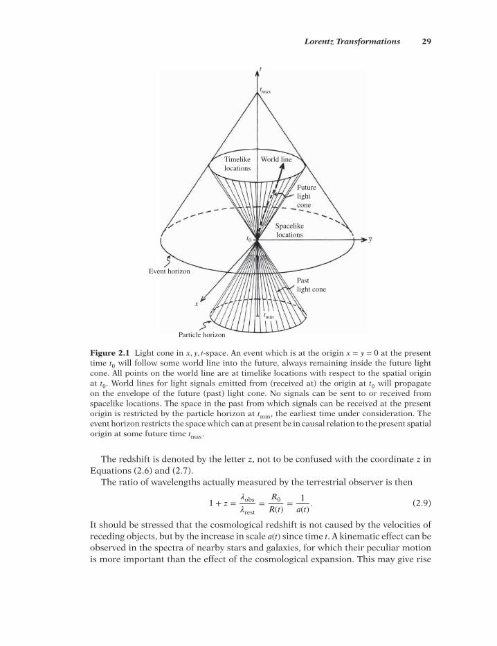
Lorentz Transformations 29
World lineTimelikelocations
Particle horizon
x
Pastlight cone
Event horizon
Spacelikelocations
Futurelightcone
t0
tmax
tmin
t
y
Figure 2.1 Light cone in 𝑥, 𝑦, 𝑡-space. An event which is at the origin 𝑥 = 𝑦 = 0 at the presenttime 𝑡0 will follow some world line into the future, always remaining inside the future lightcone. All points on the world line are at timelike locations with respect to the spatial originat 𝑡0. World lines for light signals emitted from (received at) the origin at 𝑡0 will propagateon the envelope of the future (past) light cone. No signals can be sent to or received fromspacelike locations. The space in the past from which signals can be received at the presentorigin is restricted by the particle horizon at 𝑡min, the earliest time under consideration. Theevent horizon restricts the space which can at present be in causal relation to the present spatialorigin at some future time 𝑡max.
The redshift is denoted by the letter 𝑧, not to be confused with the coordinate 𝑧 inEquations (2.6) and (2.7).
The ratio of wavelengths actually measured by the terrestrial observer is then
1 + 𝑧 =𝜆obs
𝜆rest=
𝑅0
𝑅(𝑡)= 1𝑎(𝑡)
. (2.9)
It should be stressed that the cosmological redshift is not caused by the velocities ofreceding objects, but by the increase in scale 𝑎(𝑡) since time 𝑡. A kinematic effect can beobserved in the spectra of nearby stars and galaxies, for which their peculiar motionis more important than the effect of the cosmological expansion. This may give rise

30 Special Relativity
to a Doppler redshift for a receding source, and to a corresponding blueshift for anapproaching source.
Actually, the light cones in Figure 2.1 need to be modified for an expanding uni-verse. A scale factor 𝑎(𝑡) that increases with time implies that light will travel a dis-tance greater than ct during time 𝑡. Consequently, the straight lines defining the conewill be curved outwards.
2.2 Metrics of Curved Space-time
In Newton’s time the laws of physics were considered to operate in a flat Euclideanspace, in which spatial distance could be measured on an infinite and immovablethree-dimensional grid, and time was a parameter marked out on a linear scale run-ning from infinite past to infinite future. But Newton could not answer the questionof how to identify which inertial frame was at rest relative to this absolute space. Inhis days the solar frame could have been chosen, but today we know that the SolarSystem orbits the Galactic center, the Galaxy is in motion relative to the local galaxygroup, which in turn is in motion relative to the Hydra–Centaurus cluster, and thewhole Universe is expanding.
The geometry of curved spaces was studied in the nineteenth century by Gauss,Riemann and others. Riemann realized that Euclidean geometry was just a partic-ular choice suited to flat space, but not necessarily correct in the space we inhabit.And Mach realized that one had to abandon the concept of absolute space alto-gether. Einstein learned about tensors from his friend Marcel Grossman, and usedthese key quantities to go from flat Euclidean three-dimensional space to curvedMinkowskian four-dimensional space in which physical quantities are described byinvariants. Tensors are quantities which provide generally valid relations between dif-ferent four-vectors.
Euclidean Space. Let us consider how to describe distance in three-space. The pathfollowed by a free body obeying Newton’s first law of motion can suitably be describedby expressing its spatial coordinates as functions of time: 𝑥(𝑡), 𝑦(𝑡), 𝑧(𝑡). Time is thentreated as an absolute parameter and not as a coordinate. This path represents theshortest distance between any two points along it, and it is called a geodesic of thespace. As is well known, in Euclidean space the geodesics are straight lines. Note thatthe definition of a geodesic does not involve any particular coordinate system.
If one replaces the components 𝑥, 𝑦, 𝑧 of the distance vector l by 𝑥1, 𝑥2, 𝑥3, thispermits a more compact notation of the Pythagorean squared distance 𝑙2 in the metric[Equation (2.6)]
𝑙2 = (𝑥1)2 + (𝑥2)2 + (𝑥3)2 =
3∑𝑖,𝑗=1
𝑔ij𝑥𝑖𝑥𝑗 ≡ 𝑔ij𝑥
𝑖𝑥𝑗. (2.10)
The quantities 𝑔ij are the nine components of the metric tensor g, which contains allthe information about the intrinsic geometry of this three-space. In the last step we

Metrics of Curved Space-time 31
C
θ
ϕ
P
z
R
x
y
S
r
Figure 2.2 A two-sphere on which points are specified by coordinates (𝜃, 𝜙).
have used the convention to leave out the summation sign; it is then implied thatsummation is carried out over repeated indices. One commonly uses Roman letters inthe indices when only the spatial components 𝑥𝑖, 𝑖 = 1,2,3, are implied, and Greek let-ters when all the four space-time coordinates 𝑥𝜇, 𝜇 = 0,1,2,3, are implied. Orthogonalcoordinate systems have diagonal metric tensors and this is all that we will encounter.The components of g in flat Euclidean three-space are
𝑔ij = 𝛿ij,
where 𝛿ij is the usual Kronecker delta.The same flat space could equally well be mapped by, for example, spherical or
cylindrical coordinates. The components 𝑔ij of the metric tensor would be different,but Equation (2.10) would hold unchanged. For instance, choosing spherical coordi-nates 𝑅, 𝜃, 𝜙 as in Figure 2.2,
𝑥 = 𝑅 sin 𝜃 sin𝜙, 𝑦 = 𝑅 sin 𝜃 cos𝜙, 𝑧 = 𝑅 cos 𝜃, (2.11)
d𝑙2 takes the explicit form
d𝑙2 = d𝑅2 + 𝑅2 d𝜃2 + 𝑅2 sin2𝜃 d𝜙2
. (2.12)
Geodesics in this space obey Newton’s first law of motion, which may be written as
R = 0. (2.13)
Dots indicate time derivatives.
Minkowski Space-time. In special relativity, symmetry between spatial coordinatesand time is achieved, as is evident from the Minkowski metric (2.7) describing a flatspace-time in four Cartesian coordinates. In tensor notation the Minkowski metric

32 Special Relativity
includes the coordinate d𝑥0 ≡ 𝑐 d𝑡 so that the invariant line element in Equation (2.7)can be written
d𝑠2 = 𝑐2 d𝜏2 = 𝑔𝜇𝜈
d𝑥𝜇 d𝑥𝜈. (2.14)
The 16 components of g in flat Minkowski space-time are given by the diagonal matrix𝜂𝜇𝜈
, a generalization of the Kronecker delta function to four-space-time,
𝜂00 = 1, 𝜂jj = −1, 𝑗 = 1,2,3, (2.15)
all nondiagonal components vanishing. The choice of signs in the definition of 𝜂𝜇𝜈
isnot standardized in the literature, but we shall use Equation (2.15).
The path of a body, or its world line, is then described by the four coordinate func-tions 𝑥(𝜏), 𝑦(𝜏), 𝑧(𝜏), 𝑡(𝜏), where the proper time 𝜏 is a new absolute parameter, aninvariant under Lorentz transformations. A geodesic in the Minkowski space-time isalso a straight line, given by the equations
d2𝑡
d𝜏2= 0, d2R
d𝜏2= 0. (2.16)
In the spherical coordinates [Equation (2.11)] the Minkowski metric [Equa-tion (2.7)] takes the form
d𝑠2 = 𝑐2 d𝑡2 − d𝑙2 = 𝑐2 d𝑡2 − d𝑅2 − 𝑅2 d𝜃2 − 𝑅2sin2𝜃 d𝜙2
. (2.17)
An example of a curved space is the two-dimensional surface of a sphere with radius𝑅 obeying the equation
𝑥2 + 𝑦2 + 𝑧2 = 𝑅2
. (2.18)
This surface is called a two-sphere.Combining Equations (2.6) and (2.18) we see that one coordinate is really super-
fluous, for instance 𝑧, so that the spatial metric [Equation (2.6)] can be written
d𝑙2 = d𝑥2 + d𝑦2 + (𝑥 d𝑥 + 𝑦 d𝑦)2
𝑅2 − 𝑥2 − 𝑦2. (2.19)
This metric describes spatial distances on a two-dimensional surface embedded inthree-space, but the third dimension is not needed to measure a distance on the sur-face. Note that 𝑅 is not a third coordinate, but a constant everywhere on the surface.
Thus measurements of distances depend on the geometric properties of space, ashas been known to navigators ever since Earth was understood to be spherical. Thegeodesics on a sphere are great circles, and the metric is
d𝑙2 = 𝑅2 d𝜃2 + 𝑅2sin2𝜃 d𝜙2
. (2.20)
Near the poles where 𝜃 = 0∘ or 𝜃 = 180∘ the local distance would depend very littleon changes in longitude 𝜙. No point on this surface is preferred, so it can corre-spond to a Copernican homogeneous and isotropic two-dimensional universe whichis unbounded, yet finite.
Let us write Equation (2.20) in the matrix form
d𝑙2 =(d𝜃 d𝜙
)g(
d𝜃d𝜙
), (2.21)

Metrics of Curved Space-time 33
where the metric matrix is
g =(𝑅2 00 𝑅2 sin2
𝜃
). (2.22)
The ‘two-volume’ or area 𝐴 of the two-sphere in Figure 2.2 can then be written
𝐴 =∫
2𝜋
0d𝜙
∫
𝜋
0d𝜃
√det g =
∫
2𝜋
0d𝜙
∫
𝜋
0d𝜃 𝑅2 sin 𝜃 = 4𝜋𝑅2
, (2.23)
as expected.In Euclidean three-space parallel lines of infinite length never cross, but this could
not be proved in Euclidean geometry, so it had to be asserted without proof, the parallelaxiom. The two-sphere belongs to the class of Riemannian curved spaces which arelocally flat: a small portion of the surface can be approximated by its tangential plane.Lines in this plane which are parallel locally do cross when extended far enough, asrequired for geodesics on the surface of a sphere.
Gaussian Curvature. The deviation of a curved surface from flatness can also bedetermined from the length of the circumference of a circle. Choose a point ‘P’ onthe surface and draw the locus corresponding to a fixed distance 𝑠 from that point. Ifthe surface is flat, a plane, the locus is a circle and 𝑠 is its radius. On a two-sphere ofradius 𝑅 the locus is also a circle, see Figure 2.2, but the distance 𝑠 is measured alonga geodesic. The angle subtended by 𝑠 at the center of the sphere is 𝑠∕𝑅, so the radiusof the circle is 𝑟 = 𝑅 sin (𝑠∕𝑅). Its circumference is then
𝐶 = 2𝜋𝑅 sin(𝑠∕𝑅) = 2𝜋𝑠(
1 − 𝑠2
6𝑅2+ · · ·
). (2.24)
Carl Friedrich Gauss (1777–1855) discovered an invariant characterizing the cur-vature of two-surfaces, the Gaussian curvature 𝐾. Although 𝐾 can be given by a com-pletely general formula independent of the coordinate system (see, e.g., [1]), it is mostsimply described in an orthogonal system 𝑥, 𝑦. Let the radius of curvature along the𝑥-axis be 𝑅
𝑥(𝑥) and along the 𝑦-axis be 𝑅
𝑦(𝑦). Then the Gaussian curvature at the point
(𝑥0, 𝑦0) is
𝐾 = 1∕𝑅𝑥(𝑥0)𝑅𝑦(𝑦0). (2.25)
On a two-sphere 𝑅𝑥= 𝑅
𝑦= 𝑅, so 𝐾 = 𝑅−2 everywhere. Inserting this into Equa-
tion (2.24) we obtain, in the limit of small 𝑠,
𝐾 = 3𝜋lim𝑠→0
(2𝜋𝑠 − 𝐶𝑠3
). (2.26)
This expression is true for any two-surface, and it is in fact the only invariant that canbe defined.
Whether we live in three or more dimensions, and whether our space is flat orcurved, is really a physically testable property of space. Gauss actually proceeded toinvestigate this by measuring the angles in a triangle formed by three distant moun-tain peaks. If space were Euclidean the value would be 180∘, but if the surface had
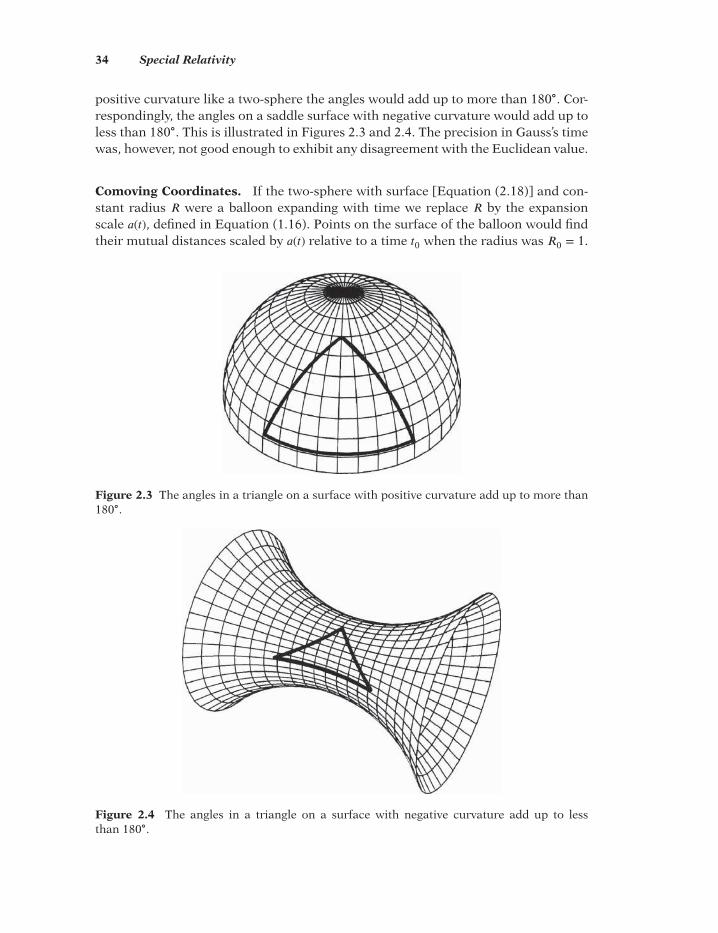
34 Special Relativity
positive curvature like a two-sphere the angles would add up to more than 180∘. Cor-respondingly, the angles on a saddle surface with negative curvature would add up toless than 180∘. This is illustrated in Figures 2.3 and 2.4. The precision in Gauss’s timewas, however, not good enough to exhibit any disagreement with the Euclidean value.
Comoving Coordinates. If the two-sphere with surface [Equation (2.18)] and con-stant radius 𝑅 were a balloon expanding with time we replace 𝑅 by the expansionscale 𝑎(𝑡), defined in Equation (1.16). Points on the surface of the balloon would findtheir mutual distances scaled by 𝑎(𝑡) relative to a time 𝑡0 when the radius was 𝑅0 = 1.
Figure 2.3 The angles in a triangle on a surface with positive curvature add up to more than180∘.
Figure 2.4 The angles in a triangle on a surface with negative curvature add up to lessthan 180∘.

Metrics of Curved Space-time 35
An observer located at any one point would see all the other points recede radially.This is exactly how we see distant galaxies except that we are not on a two-sphere but,as we shall see, on a spatially curved three-surface with the cosmic scale factor 𝑎(𝑡).
Suppose this observer wants to make a map of all the points on the expandingsurface. It is then no longer convenient to use coordinates dependent on 𝑎(𝑡) as inEquations (2.12) and (2.20), because the map would quickly be outdated. Instead itis convenient to factor out the cosmic expansion and replace 𝑎 by 𝑎(𝑡)𝜎, where 𝜎 is adimensionless comoving coordinate, thus
d𝑙2 = 𝑎2(𝑡)(d𝜎2 + 𝜎2 d𝜃2 + 𝜎2sin2𝜃 d𝜙2). (2.27)
Returning to the space we inhabit, we manifestly observe that there are threespatial coordinates, so our space must have at least one dimension more than atwo-sphere. It is easy to generalize from the curved two-dimensional manifold (sur-face) [Equation (2.18)] embedded in three-space to the curved three-dimensionalmanifold (hypersurface)
𝑥2 + 𝑦2 + 𝑧2 +𝑤2 = 𝑅2 (2.28)
of a three-sphere (hypersphere) embedded in Euclidean four-space with coordinates𝑥, 𝑦, 𝑧 and a fourth fictitious space coordinate 𝑤.
Just as the metric in Equation (2.19) could be written without explicit use of 𝑧, themetric on the three-sphere in Equation (2.28) can be written without use of 𝑤,
d𝑙2 = d𝑥2 + d𝑦2 + d𝑧2 + (𝑥 d𝑥 + 𝑦 d𝑦 + 𝑧 d𝑧)2
𝑅2 − 𝑥2 − 𝑦2 − 𝑧2, (2.29)
or, in the more convenient spherical coordinates used in Equation (2.27),
d𝑙2 = 𝑅2(𝑡)(
𝑅2 d𝜎2
𝑅2 − (𝑅𝜎)2+ 𝜎2d𝜃2 + 𝜎2sin2
𝜃 d𝜙2). (2.30)
Note that the introduction of the comoving coordinate 𝜎 in Equation (2.27) does notaffect the parameter 𝑅 defining the hypersurface in Equation (2.28). No point is pre-ferred on the manifold [Equation (2.28)], and hence it can describe a spatially homo-geneous and isotropic three-dimensional universe in accord with the cosmologicalprinciple.
Another example of a curved Riemannian two-space is the surface of a hyperboloidobtained by changing the sign of 𝑅2 in Equation (2.18). The geodesics are hyperbolas,the surface is also unbounded, but in contrast to the spherical surface it is infinitein extent. It can also be generalized to a three-dimensional curved hypersurface, athree-hyperboloid, defined by Equation (2.28) with 𝑅2 replaced by −𝑅2.
The Gaussian curvature of all geodesic three-surfaces in Euclidean four-space is
𝐾 = 𝑘∕𝑅2, (2.31)
where the curvature parameter 𝑘 can take the values +1, 0, −1, corresponding to thethree-sphere, flat three-space, and the three-hyperboloid, respectively. Actually, 𝑘 cantake any positive or negative value, because we can always rescale 𝜎 to take accountof different values of 𝑘.
36 Special Relativity
The Robertson–Walker Metric. Let us now include the time coordinate 𝑡, the cos-mic expansion scale 𝑎(𝑡) and the curvature parameter 𝑘 in Equation (2.29). We thenobtain the complete metric derived by Howard Robertson and Arthur Walker in 1934:
d𝑠2 = 𝑐2 d𝑡2 − d𝑙2 = 𝑐2 d𝑡2 − 𝑎(𝑡)2(
d𝜎2
1 − 𝑘𝜎2+ 𝜎2d𝜃2 + 𝜎2sin2
𝜃 d𝜙2). (2.32)
In the tensor notation of Equation (2.14) the components of the Robertson–Walkermetric g are obviously
𝑔00 = 1, 𝑔11 = − 𝑎2(𝑡)
1 − 𝑘𝜎2, 𝑔22 = −𝑎2(𝑡)𝜎2
, 𝑔33 = −𝑎2(𝑡)𝜎2sin2𝜃. (2.33)
Equation (2.32) is the most general metric for a four-dimensional space-time whichis homogeneous and isotropic at a given time. It then will always remain homogeneousand isotropic, because a galaxy at the point (𝜎, 𝜃, 𝜙) will always remain at that point,only the scale of spatial distances 𝑎(𝑡) changing with time. The displacements will bed𝜎 = d𝜃 = d𝜙 = 0 and the metric equation will reduce to
d𝑠2 = 𝑐2 d𝑡2. (2.34)
For this reason one calls such an expanding frame a comoving frame. A metric with𝑘 = 0 is called flat.
An observer at rest in the comoving frame is called a fundamental observer. If theUniverse appears to be homogeneous to him/her, it must also be isotropic. But anotherobserver located at the same point and in relative motion with respect to the funda-mental observer does not see the Universe as isotropic. Thus the comoving frame isreally a preferred frame, and a very convenient one, as we shall see later in conjunctionwith the cosmic background radiation. Let us note here that a fundamental observermay find that not all astronomical bodies recede radially; a body at motion relative tothe comoving coordinates (𝜎, 𝜃, 𝜙) will exhibit peculiar motion in other directions.
Another convenient comoving coordinate is 𝜒 , defined by integrating over
d𝜒 = d𝜎√1 − 𝑘𝜎2
. (2.35)
Inserting this into Equation (2.32), the metric can be written
d𝑠2 = 𝑐2 d𝑡2 − 𝑎2(𝑡)[d𝜒2 + 𝑆2𝑘(𝜒)(d𝜃2 + sin2
𝜃 d𝜙2)], (2.36)
where𝑆𝑘(𝜒) ≡ 𝜎
and𝑆1(𝜒) = sin𝜒, 𝑆0(𝜒) = 𝜒, 𝑆−1(𝜒) = sinh𝜒. (2.37)
We shall use the metrics in Equations (2.32) and (2.36) interchangeably since bothoffer advantages. In so doing I have take great care of not introducing contradictions.
Let us briefly digress to define what is sometimes called cosmic time. In an expand-ing universe the galaxies are all moving away from each other (let us ignore peculiar

Relativistic Distance Measures 37
velocities) with clocks running at different local time, but from our vantage pointwe would like to have a time value applicable to all of them. If one postulates, withHermann Weyl (1885–1955), that the expansion is so regular that the world lines ofthe galaxies form a nonintersecting and diverging three-bundle of geodesics, and thatone can define spacelike hypersurfaces which are orthogonal to all of them. Then eachsuch hypersurface can be labeled by a constant value of the time coordinate 𝑥0, andusing this value one can meaningfully talk about cosmic epochs for the totality of theUniverse. This construction in space-time does not imply the choice of a preferredtime in conflict with special relativity.
2.3 Relativistic Distance Measures
Let us consider how to measure distances in our comoving frame in which we areat the origin. The comoving distance from us to a galaxy at comoving coordinates(𝜎,0,0) is not an observable because a distant galaxy can only be observed by the lightit emitted at an earlier time 𝑡 < 𝑡0. In a space-time described by the Robertson–Walkermetric the light signal propagates along the geodesic d𝑠2 = 0. Choosing d𝜃2 = d𝜙2 = 0,it follows from Equation (2.36) that this geodesic is defined by
𝑐2 d𝑡2 − 𝑎2(𝑡) d𝜒2 = 0.
It follows that 𝜒 can be written
𝜒 = 𝑐∫
𝑡0
𝑡
d𝑡𝑎(𝑡)
. (2.38)
The time integral in Equation (2.38) is called the conformal time.
Proper Distance. Let us now define the proper distance 𝑑P at time 𝑡0 (when the cos-mic scale is 𝑎(𝑡0) = 1) to the galaxy at (𝜎,0,0). This is a function of 𝜎 and of the intrinsicgeometry of space-time and the value of 𝑘. Integrating the spatial distance d𝑙 ≡ |dl| inEquation (2.32) from 0 to 𝑑P we find
𝑑P =∫
𝜎
0
d𝜎√1 − 𝑘𝜎2
= 1√𝑘
sin−1(√𝑘𝜎) = 𝜒. (2.39)
For flat space 𝑘 = 0 we find the expected result 𝑑P = 𝜎. In a universe with curvature𝑘 = +1 and scale 𝑎 then Equation (2.39) becomes
𝑑P = 𝑎𝜒 = 𝑎 sin−1𝜎 or 𝜎 = sin(𝑑P∕𝑎).
As the distance 𝑑P increases from 0 to 12𝜋𝑎, 𝜎 also increases from 0 to its maximum
value 1. However, when 𝑑P increases from 12𝜋𝑎 to 𝜋𝑎, 𝜎 decreases back to 0. Thus,
travelling a distance 𝑑P = 𝜋𝑎 through the curved three-space brings us to the other endof the Universe. Travelling on from 𝑑P = 𝜋𝑎 to 𝑑P = 2𝜋𝑎 brings us back to the point ofdeparture. In this sense a universe with positive curvature is closed.

38 Special Relativity
Similarly, the area of a three-sphere centered at the origin and going through thegalaxy at 𝜎 is
𝐴 = 4𝜋𝑎2𝜎
2 = 4𝜋𝑎2sin2(𝑑P∕𝑎). (2.40)
Clearly, 𝐴 goes through a maximum when 𝑑P = 12𝜋𝑎, and decreases back to 0 when 𝑑P
reaches 𝜋𝑎. Note that𝐴∕4 equals the area enclosed by the circle formed by intersectinga two-sphere of radius𝑅with a horizontal plane, as shown in Figure 2.1. The intersec-tion with an equatorial plane results in the circle enclosing maximal area, 𝐴∕4 = 𝜋𝑅2,all other intersections making smaller circles. A plane tangential at either pole has nointersection, thus the corresponding ‘circle’ has zero area.
The volume of the three-sphere in Equation (2.28) can then be written in analogywith Equation (2.23),
𝑉 = 2∫
2𝜋
0d𝜙
∫
𝜋
0d𝜃
∫
1
0d𝜎
√det gRW, (2.41)
where the determinant of the spatial part of the Robertson–Walker metric matrix gRW
is now
det gRW = 𝑎6 𝜎4
1 − 𝜎2sin2
𝜃. (2.42)
The factor 2 in Equation (2.41) comes from the sign ambiguity of 𝑤 in Equa-tion (2.28). Both signs represent a complete solution. Inserting Equation (2.42) intoEquation (2.41) one finds the volume of the three-sphere:
𝑉 = 2𝜋2𝑎
3. (2.43)
The hyperbolic case is different. Setting 𝑘 = −1, the function in Equation (2.39) isi−1sin−1i𝜎 ≡ sinh−1
𝜎, thus
𝑑P = 𝑎𝜒 = 𝑎 sinh−1𝜎 or 𝜎 = sinh(𝑑P∕𝑎). (2.44)
Clearly this space is open because 𝜎 grows indefinitely with 𝑑P. The area of thethree-hyperboloid through the galaxy at 𝜎 is
𝐴 = 4𝜋𝑎2𝜎
2 = 4𝜋𝑎2sinh2(𝑑P∕𝑎). (2.45)
Let us differentiate 𝑑P in Equation (2.39) with respect to time, noting that 𝜎 is a con-stant since it is a comoving coordinate. We then obtain the Hubble flow 𝑣 experiencedby a galaxy at distance 𝑑P:
𝑣 = ��P = ��(𝑡)∫
𝜎
0
d𝜎√1 − 𝑘𝜎2
= ��(𝑡)𝑎(𝑡)
𝑑P. (2.46)
Thus the Hubble flow is proportional to distance, and Hubble’s law emerges in a formmore general than Equation (1.20):
𝐻(𝑡) = ��(𝑡)𝑎(𝑡)
. (2.47)
Recall that 𝑣 is the velocity of expansion of the space-time geometry. A galaxy withzero comoving velocity would appear to have a radial recession velocity 𝑣 because ofthe expansion.

Relativistic Distance Measures 39
Particle and Event Horizons. In Equation (1.14) we defined the Hubble radius 𝑟Has the distance reached in one Hubble time, 𝜏H, by a light signal propagating along astraight line in flat, static space. Let us define the particle horizon 𝜎ph or 𝜒ph (also objecthorizon) as the largest comoving spatial distance from which a light signal could havereached us if it was emitted at time 𝑡 = 𝑡min < 𝑡0. Thus it delimits the size of that partof the Universe that has come into causal contact since time 𝑡min. If the past time 𝑡 isset equal to the last scattering time (the time when the Universe became transparentto light, and thus the earliest time anything was visible, as we will discuss in a laterchapter) the particle horizon delimits the visible Universe. From Equation (2.38),
𝜒ph = 𝑐∫
𝑡0
𝑡min
d𝑡𝑎(𝑡)
, (2.48)
and from the notation in Equation (2.37),
𝜎ph = 𝑆𝑘(𝜒ph).
A particle horizon exists if 𝑡min is in the finite past. Clearly the value of 𝜎ph dependssensitively on the behavior of the scale of the Universe at that time, 𝑎(𝑡ph).
If 𝑘 ⩾ 0, the proper distance (subscript ‘P’) to the particle horizon (subscript ‘ph’)at time 𝑡 is
𝑑P,ph = 𝑎(𝑡)𝜒ph. (2.49)
Note that 𝑑P equals the Hubble radius 𝑟H = 𝑐∕𝐻0 when 𝑘 = 0 and the scale is a con-stant, 𝑎(𝑡) = 𝑎. When 𝑘 = −1 the Universe is open, and 𝑑P,ph cannot be interpreted as ameasure of its size.
In an analogous way, the comoving distance 𝜎eh to the event horizon is defined asthe spatially most distant present event from which a world line can ever reach ourworld line. By ‘ever’ we mean a finite future time, 𝑡max:
𝜒eh ≡ 𝑐∫
𝑡max
𝑡0
d𝑡𝑎(𝑡)
. (2.50)
The particle horizon 𝜎ph at time 𝑡0 lies on our past light cone, but with time our particlehorizon will broaden so that the light cone at 𝑡0 will move inside the light cone at 𝑡 > 𝑡0(see Figure 2.1). The event horizon at this moment can only be specified given the timedistance to the ultimate future, 𝑡max. Only at 𝑡max will our past light cone encompassthe present event horizon. Thus the event horizon is our ultimate particle horizon.Comoving bodies at the Hubble radius recede with velocity c, but the particle horizonitself recedes even faster. From
d(𝐻𝑑P,ph)∕d𝑡 = ��𝑑P,ph +𝐻��P,ph = 0,
and making use of the deceleration parameter 𝑞, defined by
𝑞 = −𝑎����2
= − ��
𝑎𝐻2, (2.51)
one finds
��P,ph = 𝑐(𝑞 + 1). (2.52)

40 Special Relativity
Thus when the particle horizon grows with time, bodies which were at spacelike dis-tances at earlier times enter into the light cone.
The integrands in Equations (2.48) and (2.50) are obviously the same, only theintegration limits are different, showing that the two horizons correspond to differentconformal times. If 𝑡min = 0, the integral in Equation (2.48) may well diverge, in whichcase there is no particle horizon. Depending on the future behavior of 𝑎(𝑡), an eventhorizon may or may not exist. If the integral diverges as 𝑡 → ∞, every event will sooneror later enter the event horizon. The event horizon is then a function of waiting timeonly, but there exists no event horizon at 𝑡 = ∞. But if 𝑎(𝑡) accelerates, so that distantparts of the Universe recede faster than light, then there will be an ultimate eventhorizon. We shall see later that 𝑎(𝑡) indeed appears to accelerate.
Redshift and Proper Distance. In Equation (1.20) in the previous chapter weparametrized the rate of expansion �� by the Hubble constant 𝐻0. It actually appearedas a dynamical parameter in the lowest-order Taylor expansion of 𝑎(𝑡), Equation (1.18).If we allow 𝐻(𝑡) to have some mild time dependence, that would correspond to intro-ducing another dynamical parameter along with the next term in the Taylor expan-sion. Thus adding the second-order term to Equation (1.18), we have for 𝑎(𝑡),
𝑎(𝑡) ≈ 1 − ��0(𝑡0 − 𝑡) +12��0(𝑡0 − 𝑡)2. (2.53)
Making use of the definition in Equation (2.47), the second-order expansion for thedimensionless scale factor is
𝑎(𝑡) ≈ 1 −𝐻0(𝑡0 − 𝑡) +12��0(𝑡0 − 𝑡)2. (2.54)
As long as the observational information is limited to the first time derivative ��0,no further terms can be added to these expansions. To account for ��0, we shall nowmake use of the present value of the deceleration parameter in Equation (2.51), 𝑞0.Then the lowest-order expression for the cosmological redshift, Equation (1.18), canbe replaced by
𝑧(𝑡) = (𝑎(𝑡)−1 − 1)
=[1 −𝐻0(𝑡 − 𝑡0) −
12𝑞0𝐻
20 (𝑡 − 𝑡0)
2]−1
− 1
≈ −𝐻0(𝑡 − 𝑡0) +(
1 + 12𝑞0
)𝐻
20 (𝑡 − 𝑡0)
2.
This expression can further be inverted to express 𝐻0(𝑡 − 𝑡0) as a function of the red-shift to second order:
𝐻0(𝑡0 − 𝑡) ≈ 𝑧 − (1 + 12𝑞0)𝑧2
. (2.55)
Let us now find the proper distance 𝑑P to an object at redshift 𝑧 in this approxima-tion. Eliminating 𝜒 in Equations (2.38) and (2.39) we have
𝑑P = 𝑐∫
𝑡0
𝑡
d𝑡𝑎(𝑡)
.
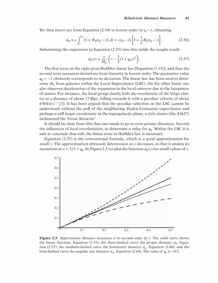
Relativistic Distance Measures 41
We then insert 𝑎(𝑡) from Equation (2.54) to lowest order in 𝑡0 − 𝑡, obtaining
𝑑P ≈ 𝑐∫
𝑡0
𝑡
[1 +𝐻0(𝑡0 − 𝑡)] d𝑡 = 𝑐(𝑡0 − 𝑡)[1 + 1
2𝐻0(𝑡0 − 𝑡)
]. (2.56)
Substituting the expression in Equation (2.55) into this yields the sought result:
𝑑P(𝑧) ≈𝑐
𝐻0
(𝑧 − 1
2(1 + 𝑞0)𝑧2
). (2.57)
The first term on the right gives Hubble’s linear law [Equation (1.15)], and thus thesecond term measures deviations from linearity to lowest order. The parameter value𝑞0 = −1 obviously corresponds to no deviation. The linear law has been used to deter-mine 𝐻0 from galaxies within the Local Supercluster (LSC). On the other hand, onealso observes deceleration of the expansion in the local universe due to the lumpinessof matter. For instance, the local group clearly feels the overdensity of the Virgo clus-ter at a distance of about 17 Mpc, falling towards it with a peculiar velocity of about630 km s−1 [3]. It has been argued that the peculiar velocities in the LSC cannot beunderstood without the pull of the neighboring Hydra–Centaurus supercluster andperhaps a still larger overdensity in the supergalactic plane, a rich cluster (the A3627)nicknamed the ‘Great Attractor’.
It should be clear from this that one needs to go to even greater distances, beyondthe influences of local overdensities, to determine a value for 𝑞0. Within the LSC it issafe to conclude that only the linear term in Hubble’s law is necessary.
Equation (2.57) is the conventional formula, which is a good approximation forsmall 𝑧. The approximation obviously deteriorates as 𝑧 increases, so that it attains itsmaximum at 𝑧 = 1∕1 + 𝑞0. In Figure 2.5 we plot the function 𝑑P(𝑧) for small values of 𝑧.
0.7
0.6
0.5
0.4
0.3
0.2
0.1
0.1 0.2 0.3 0.4 0.5
Figure 2.5 Approximate distance measures 𝑑 to second order in 𝑧. The solid curve showsthe linear function, Equation (1.15); the short-dashed curve the proper distance 𝑑P, Equa-tion (2.57); the medium-dashed curve the luminosity distance 𝑑L, Equation (2.60); and thelong-dashed curve the angular size distance 𝑑A, Equation (2.64). The value of 𝑞0 is −0.5.

42 Special Relativity
Redshift and Luminosity Distance. Consider an astronomical object emitting pho-tons isotropically with power or absolute luminosity 𝐿. At the luminosity distance 𝑑L
from the object we observe only the fraction 𝐵s, its surface brightness, given by theinverse-square distance law
𝐵s =𝐿
4𝜋𝑑2L
. (2.58)
Let us now find 𝑑L as a function of 𝑧 in such a way that the Euclidean inverse-squarelaw [Equation (2.58)] is preserved. If the Universe does not expand and the object isstationary at proper distance 𝑑P, a telescope with area 𝐴will receive a fraction 𝐴∕4𝜋𝑑2
Pof the photons. But in a universe characterized by an expansion 𝑎(𝑡), the object isnot stationary, so the energy of photons emitted at time 𝑡e is redshifted by the factor(1 + 𝑧) = 𝑎−1(𝑡e). Moreover, the arrival rate of the photons suffers time dilation byanother factor (1 + 𝑧), often called the energy effect. The apparent brightness 𝐵a is thengiven by
𝐵a = 𝐿
4𝜋𝑑2P(1 + 𝑧)2
. (2.59)
Equating 𝐵a = 𝐵s one sees that 𝑑L = 𝑑P(1 + 𝑧), and making use of the expression inEquation (2.57) one obtains
𝑑L(𝑧) ≈𝑐
𝐻0
(𝑧 + 1
2(1 − 𝑞0)𝑧2
). (2.60)
In Figure 2.5 we plot the function 𝑑L(𝑧) for small values of 𝑧.Astronomers usually replace 𝐿 and 𝐵 by two empirically defined quantities, abso-
lute magnitude 𝑀 of a luminous object and apparent magnitude 𝑚. The replacementrule is
𝑚 −𝑀 = −5 + 5 log 𝑑L, (2.61)
where 𝑑L is expressed in parsecs (pc) and the logarithm is to base 10. For example, ifone knows the distance 𝑑L to a galaxy hosting a supernova, its absolute magnitude 𝑀can be obtained from observations of its apparent magnitude 𝑚.
Parallax Distance. Some measurements of 𝐻0 depend directly on the calibration oflocal distance indicators which form the first rung of a ladder of distance measure-ments. The distances to relatively nearby stars can be measured by the trigonometricalparallax up to about 30 pc away (see Table A.1 in the appendix for cosmic distances).This is the difference in angular position of a star as seen from Earth when at oppositepoints in its circumsolar orbit. The parallax distance 𝑑p is defined as
𝑑p = 𝑑P∕√
1 − 𝑘𝜎2. (2.62)
It has been found that most stars in the Galaxy for which we know the luminosityfrom a kinematic distance determination exhibit a relationship between surface tem-perature or color and absolute luminosity, the Hertzsprung–Russell relation. Thesestars are called main-sequence stars and they sit on a fairly well-defined curve in the

Relativistic Distance Measures 43
temperature–luminosity plot. Temperature can be determined from color—note thatastronomers define color as the logarithm of the ratio of the apparent brightnesses inthe red and the blue wavelength bands. Cool stars with surface temperature around3000 K are infrared, thus the part of their spectrum which is in the visible is domi-nantly red. Hot stars with surface temperature around 12 000 K are ultraviolet, thusthe part of their spectrum which is in the visible is dominantly blue. The Sun, with asurface temperature of 5700 K, radiates mainly in the visible, thus its color is a blendedwhite, slightly yellow. Most main-sequence stars like our Sun are in a prolonged stateof steady burning of hydrogen into helium.
Once this empirical temperature–luminosity relation is established, it can be usedthe other way around to derive distances to farther main-sequence stars: from theircolor one obtains the luminosity which subsequently determines 𝑑L. By this methodone gets a second rung in a ladder of estimates which covers distances within ourGalaxy.
Angular Size Distance. Yet another measure of distance is the angular size distance𝑑A. In Euclidean space an object of size 𝐷 that is at distance 𝑑A will subtend an angle2𝜃 such that
2𝜃 = tan(𝐷∕𝑑A) ≈ 𝐷∕𝑑A,
where the approximation is good for small 𝜃. This can serve as the definition of 𝑑A inEuclidean space. In general relativity we can still use this equation to define a distancemeasure 𝑑A. From the metric in Equation (2.32) the radius of a source of light atcomoving distance 𝜎 is 𝐷 = 𝑎𝜎𝜃, so
𝑑A = 𝐷∕𝜃 = 𝑎𝜎 = 𝑎𝑆𝑘𝑑P. (2.63)
This definition preserves the relation between angular size and distance, a propertyof Euclidean space. But expansion of the Universe and the changing scale factor 𝑎(𝑡)means that as proper distance 𝑑P or redshift 𝑧 increases, the angular diameter distanceinitially increases but ultimately decreases. Light rays from the object detected by theobserver have been emitted when the proper distance to the object, measured at fixedworld time, was small. Because the proper distance between observer and source isincreasing faster than the speed of light, emitted light in the direction of the observeris initially moving away from the observer.
The redshift dependence of 𝑑A can be found from Equations (2.57) and (2.37) once𝑘 is known. In Figure 2.5 we plot 𝑑A for the choice 𝑘 = 0 when
𝑑A = 𝑎𝑑P =𝑑P
1 + 𝑧. (2.64)
The 𝑘 dependence makes it a useful quantity to determine cosmological parame-ters. In particular, 𝑘 is sensitive to certain combinations of well-measured parameters.
Distance Ladder Continued. As the next step on the distance ladder one choosescalibrators which are stars or astronomical systems with specific uniform properties,so called standard candles. The RR Lyrae stars all have similar absolute luminosities,

44 Special Relativity
and they are bright enough to be seen out to about 300 kpc. A very important classof standard candles are the Cepheid stars, whose absolute luminosity oscillates with aconstant period 𝑃 in such a way that log 𝑃 ∝ 1.3 log 𝐿. The period 𝑃 can be observedwith good precision, thus one obtains a value for 𝐿. Cepheids have been found withinour Galaxy where the period–luminosity relation can be calibrated by distances fromtrigonometric parallax measurements. This permits use of the period–luminosity rela-tion for distances to Cepheids within the Large Magellanic Cloud (LMC), our satellitegalaxy. At a distance of 55 kpc the LMC is the first important extragalactic landmark.
The resolution of individual stars within galaxies clearly depends on the distance tothe galaxy. This method, called surface-brightness fluctuations (SBFs), is an indicatorof relative distances to elliptical galaxies and some spirals. The internal precision ofthe method is very high, but it can be applied only out to about 70 Mpc.
Globular clusters are gravitationally bound systems of 105–106 stars forming aspherical population orbiting the center of our Galaxy. From their composition oneconcludes that they were created very early in the evolution of the Galaxy. We alreadymade use of their ages to estimate the age of the Universe in Section 1.5. Glob-ular clusters can also be seen in many other galaxies, and they are visible out to100 Mpc. Within the Galaxy their distance can be measured as described above, andone then turns to study the statistical properties of the clusters: the frequency of starsof a given luminosity, the mean luminosity, the maximum luminosity, and so on. Awell-measured cluster then becomes a standard candle with properties presumablyshared by similar clusters at all distances. Similar statistical indicators can be used tocalibrate clusters of galaxies; in particular the brightest galaxy in a cluster is a stan-dard candle useful out to 1 Gpc.
The next two important landmarks are the distances to the Virgo cluster, whichis the closest moderately rich concentrations of galaxies, and to the Coma cluster,which is one of the closest clusters of high richness. The Virgo distance has beendetermined to be 17 Mpc by the observations of galaxies containing several Cepheids,by the Hubble Space Telescope [4]. The Coma is far enough, about 100 Mpc, that itsredshift is almost entirely due to the cosmological expansion.
The existence of different methods of calibration covering similar distances is agreat help in achieving higher precision. The expansion can be verified by measuringthe surface brightness of standard candles at varying redshifts, the Tolman test. Ifthe Universe does indeed expand, the intensity of the photon signal at the detectoris further reduced by a factor (1 + 𝑧)2 due to an optical aberration which makes thesurface area of the source appear increased. Such tests have been done and they doconfirm the expansion.
The Tully–Fisher relation is a very important tool at distances which overlap thosecalibrated by Cepheids, globular clusters, galaxy clusters and several other methods.This empirical relation expresses correlations between intrinsic properties of wholespiral galaxies. It is observed that their absolute luminosity and their circular rotationvelocity 𝑣c are related by
𝐿 ∝ 𝑣4c . (2.65)

Tests of Special Relativity 45
The Tully–Fisher relation for spiral galaxies is calibrated by nearby spiral galax-ies having Cepheid calibrations, and it can then be applied to spiral galaxies outto 150 Mpc. Elliptical galaxies do not rotate, they are found to occupy a fundamen-tal plane in which an effective radius is tightly correlated with the surface brightnessinside that radius and with the central velocity dispersion of the stars. In principle,this method could be applied out to 𝑧 ≈ 1, but in practice stellar evolution effects andthe nonlinearity of Hubble’s law limit the method to 𝑧 ≲ 0.1, or about 400 Mpc.
For more details on distance measurements the reader is referred to the excellenttreatment in the book by Peacock [5].
2.4 Tests of Special Relativity
Special relativity is an inseparable part of quantum field theory which describes theworld of elementary particles with an almost incredible precision. Particle physicshas tested special relativity in thousands of different experiments without finding aflaw: the Lorentz invariance is locally exact. But at astronomical and cosmologicalscales the local Lorentz invariance has to be replaced by General Relativity. The quib-ble about whether special relativity is generally true and testable at cosmological dis-tances and time scales is therefore meaningless.
Special relativity really contains only one parameter, c, the velocity of light in vacuo,which has the dimension of length/time. Could c be variable, or is c even measurableat all? One is free to choose 𝑐 = 1 locally because that only implies a rescaling of theunits of length. To explain problematic observations the possibility of a variable speedof light has sometimes been invoked. Also Newton’s constant of gravitation, G, couldin principle be variable. Already Einstein admitted that the value of G could dependon the local strength of the gravitational field. In order to avoid trivial rescaling ofunits, one must test the simultaneous variation of c, G and the fine structure constantwhich can be combined to a dimensionless number. Note that c and G enter in thecombination 𝐺∕𝑐4 in the Einstein Equation (3.29).
A measurement of the radius of Mercury has produced no time variation of c
��
𝑐= 0 ± 2 × 10⁻¹² yr−1
. (2.66)
The white dwarf star Stein 2051B within our Galaxy also provides only a limit whencombined with the upper limit of the variability of the fine structure constant,
𝐻0��
𝑐= 0 ± 2.1 × 10⁻³ yr (2.67)
using 𝐻0 = 1.5 × 10¹⁰ yr.Determinations of the time variation of G have also given null results. The strongest
constraint due to a lunar laser ranging experiment gives
| ��𝐺| ⩽ 1.3 × 10⁻¹² yr−1
. (2.68)

46 Special Relativity
Variable speed of light is in conflict with Lorentz invariance and with Einstein’stime dilation formula in Equation (2.5). Although there have been many attemptsto test this by measuring the transverse second-order Doppler shift by Mössbauerspectroscopy, the results are claimed to be either wrong or doubtful, and in need ofimproved technology.
On the theoretical side there are interesting generalizations of the linear Lorentztransformations to uniformly accelerated or rotating frames. Some generalized trans-formations predict acceleration-dependent Doppler shift and time dilation, as well asa maximal acceleration [6, 7].
Problems
1. Starting from the postulates (i) and (ii) in Section 2.1 and the requirement thatd𝑠2 in Equation (2.1) should have the same form in the primed and unprimedcoordinates, derive the linear Lorentz transformation in Equation (2.2) and theexpression in Equation (2.3).
2. The radius of the Galaxy is 3 × 10²⁰ m. How fast would a spaceship have to travelto cross it in 300 yr as measured on board? Express your result in terms of𝛾 = 1∕
√1 − 𝑣2∕𝑐2 [7].
3. An observer sees a spaceship coming from the west at a speed of 0.6𝑐 and aspaceship coming from the east at a speed 0.8𝑐. The western spaceship sends asignal with a frequency of 104 Hz in its rest frame. What is the frequency of thesignal as perceived by the observer? If the observer sends on the signal imme-diately upon reception, what is the frequency with which the eastern spaceshipreceives the signal [7]?
4. If the eastern spaceship in the previous problem were to interpret the signal asone that is Doppler shifted because of the relative velocity between the westernand eastern spaceships, what would the eastern spaceship conclude about therelative velocity? Show that the relative velocity must be (𝑣1 + 𝑣2)∕(1 + 𝑣1𝑣2∕𝑐2),where 𝑣1 and 𝑣2 are the velocities as seen by an outside observer [7].
5. A source flashes with a frequency of 1015 Hz. The signal is reflected by a mirrormoving away from the source with speed 10 km s−1. What is the frequency of thereflected radiation as observed at the source [7]?
6. Suppose that the evolution of the Universe is described by a constant deceler-ating parameter 𝑞 = 1
2. We observe two galaxies located in opposite directions,
both at proper distance 𝑑P. What is the maximum separation between the galax-ies at which they are still causally connected? Express your result as a fractionof distance to 𝑑P. What is the observer’s particle horizon?
7. Show that the Hubble distance 𝑟H = 𝑐∕𝐻 recedes with radial velocity
��H = 𝑐(1 + 𝑞). (2.69)
8. Is the sphere defined by the Hubble radius 𝑟H inside or outside the particlehorizon?

Tests of Special Relativity 47
9. Calculate whether the following space-time intervals from the origin are space-like, timelike or lightlike: (1, 3, 0, 0); (3, 3, 0, 0); (3, -3, 0, 0); (0, 3, 0, 0); (3, 1, 0,0) [1].
10. The supernova 1987A explosion in the Large Magellanic Cloud 170 000 lightyears from Earth produced a burst of anti-neutrinos 𝜈e which were observedin terrestrial detectors. If the anti-neutrinos are massive, their velocity woulddepend on their mass as well as their energy. What is the proper time intervalbetween the emission, assumed to be instantaneous, and the arrival on Earth?Show that in the limit of vanishing mass the proper time interval is zero. Whatinformation can be derived about the anti-neutrino mass from the observationthat the energies of the anti-neutrinos ranged from 7 to 11 MeV, and the arrivaltimes showed a dispersion of 7 s?
11. The theoretical resolving power of a telescope is given by 𝛼 = 1.22𝜆∕𝐷, where 𝜆 isthe wavelength of the incoming light and𝐷 is the diameter of the mirror. Assum-ing 𝐷 = 5 m and 𝜆 = 8 × 10⁻⁷ m, determine the largest distance to a star that canbe measured by the parallax method. (In reality, atmospheric disturbances settighter limits.)
References[1] Kenyon, I. R. 1990 General relativity. Oxford University Press, Oxford.[2] Pyykkö, P. 1988 Chem. Rev. 88, 563.[3] Lynden-Bell, D. et al. 1988 Astrophys. J. 326, 19.[4] Freedman, W. L. et al. 1994 Nature 371, 757.[5] Peacock, J. A. 1999 Cosmological physics. Cambridge University Press, Cambridge.[6] Friedman, Y. and Scarr, T. 2013 Physica Scripta 87, 055004, and references therein.[7] Gasiorowicz, S. 1979 The structure of matter. Addison-Wesley, Reading, MA.


3
General Relativity
Newton’s law of gravitation, Equation (1.28), runs into serious conflict with specialrelativity in three different ways. First, there is no obvious way of rewriting it in termsof invariants, since it only contains scalars. Second, it has no explicit time dependence,so gravitational effects propagate instantaneously to every location in the Universe,in fact, also infinitely far outside the horizon of the Universe!
Third, the gravitating mass 𝑚G appearing in Equation (1.28) is totally independentof the inert mass 𝑚 appearing in Newton’s second law [Equation (2.29)], as we alreadynoted, yet for unknown reasons both masses appear to be equal to a precision of 10−13
or better (10−18 is expected soon). Clearly a theory is needed to establish a formal linkbetween them. Mach thought that the inert mass of a body was somehow linked to thegravitational mass of the whole Universe. To be rigorous, he thought that axes of localnonrotating frames, such as axes of gyroscopes, in their time-evolution precisely fol-low some average of the motion of matter in the Universe. Einstein, who was stronglyinfluenced by the ideas of Mach, called this Mach’s principle. In his early work on gen-eral relativity he considered it to be one of the basic, underlying principles, togetherwith the principles of equivalence and covariance, but in his later publications he nolonger referred to it. This may have been a misunderstanding of Einstein because, ifone carefully defines the words precisely follow and some average, Mach’s principle isa consequence of cosmology with Einstein Gravity.
Facing the above shortcomings of Newtonian mechanics and the limitations ofspecial relativity Einstein set out on a long and tedious search for a better law ofgravitation valid in the inhomogeneous gravitational field near a massive body, yetone that would reduce to Newton’s law in some limit. Realizing that the space we livein was not flat, except locally equivalent to (a patchwork of flat frames describing)a curved space-time, the law of gravitation has to be a covariant relation betweenmass density and curvature. Thus Einstein proceeded to combine the principle ofequivalence which we describe in Section 3.1 and the principle of general covariancewhich we meet in Section 3.2.
Introduction to Cosmology, Fourth Edition. Matts Roos© 2015 John Wiley & Sons, Ltd. Published 2015 by John Wiley & Sons, Ltd.
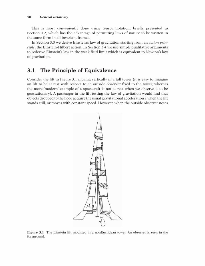
50 General Relativity
This is most conveniently done using tensor notation, briefly presented inSection 3.2, which has the advantage of permitting laws of nature to be written inthe same form in all invariant frames.
In Section 3.3 we derive Einstein’s law of gravitation starting from an action prin-ciple, the Einstein-Hilbert action. In Section 3.4 we use simple qualitative argumentsto rederive Einstein’s law in the weak field limit which is equivalent to Newton’s lawof gravitation.
3.1 The Principle of Equivalence
Consider the lift in Figure 3.1 moving vertically in a tall tower (it is easy to imaginean lift to be at rest with respect to an outside observer fixed to the tower, whereasthe more ‘modern’ example of a spacecraft is not at rest when we observe it to begeostationary). A passenger in the lift testing the law of gravitation would find thatobjects dropped to the floor acquire the usual gravitational acceleration 𝑔 when the liftstands still, or moves with constant speed. However, when the outside observer notes
Figure 3.1 The Einstein lift mounted in a nonEuclidean tower. An observer is seen in theforeground.
The Principle of Equivalence 51
that the lift is accelerating upwards, tests inside the lift reveal that the objects acquirean acceleration larger than 𝑔, and vice versa when the lift is accelerating downwards.In the limit of free fall (unpleasant to the passenger) the objects appear weightless,corresponding to zero acceleration.
Let us now replace the lift with a spacecraft with the engines turned off, locatedat some neutral point in space where all gravitational pulls cancel or are negligible:a good place is the Lagrange point, where the terrestrial and solar gravitational fieldscancel. All objects, including the pilot, would appear weightless there.
Now turning on the engines by remote radio control, the spacecraft could be accel-erated upwards so that objects on board would acquire an acceleration 𝑔 towards thefloor. The pilot would then rightly conclude that
gravitational pull and local acceleration are equivalent
and indistinguishable if no outside information is available and if 𝑚 = 𝑚G. This con-clusion forms the weak equivalence principle (WEP), which states that an observer ina gravitational field will not experience free fall as a gravitational effect, but as beingat rest in a locally accelerated frame.
A passenger in the lift measuring 𝑔 could well decide from his local observationsthat Earth’s gravitation actually does not exist, but that the lift is accelerating radiallyoutwards from Earth. This interpretation does not come into conflict with that ofanother observer on the opposite side of Earth whose frame would accelerate in theopposite direction, because that frame is only local to him/her.
The weak equivalence principle is already embodied in the Galilean equivalenceprinciple in mechanics between motion in a uniform gravitational field and a uni-formly accelerated frame of reference. What Einstein did was to generalize this to allof physics, in particular phenomena involving light.
The more general formulation is the important strong equivalence principle (SEP),which states that
to an observer in free fall in a gravitational field the results of all local exper-iments are completely independent of the magnitude of the field.
In a suitably small lift or spacecraft, curved space-time can always be approximatedby flat Minkowski space-time. In the gravitational field of Earth the gravitational accel-eration is directed toward its center. Thus the two test bodies in Figure 3.2 with aspace-like separation do not actually fall along parallels, but along different radii, sothat their separation decreases with time. This phenomenon is called the tidal effect,or sometimes the tidal force, since the test bodies move as if an attractive exchangeforce acted upon them. The classic example is the tide caused by the Moon on theoceans. The force experienced by a body of mass 𝑚 and diameter 𝑑 in gravitationalinteraction with a body of mass 𝑀 at a distance 𝑟 is proportional to the differential ofthe force of attraction [Equation (1.28])] with respect to 𝑟. Neglecting the geometricalshapes of the bodies, the tidal force is
𝐹tidal ≈ GMmd∕𝑟3
.
Thus parts of 𝑚 located at smaller distances 𝑟 feel a stronger force.

52 General Relativity
F
Figure 3.2 Tidal force 𝐹 acting between two test bodies falling freely towards the surface of agravitating body. On the right a spherical cluster of small bodies is seen to become ellipsoidalon approaching the body.
An interesting example is offered by a sphere of freely falling particles. Since thestrength of the gravitational field increases in the direction of fall, the particles in thefront of the sphere will fall faster than those in the rear. At the same time the lateralcross-section of the sphere will shrink due to the tidal effect. As a result, the spherewill be focused into an ellipsoid with the same volume. This effect is responsible forthe gravitational breakup of very nearby massive stars.
If the tidal effect is too small to be observable, the laboratory can be consideredto be local. On a larger scale the gravitational field is clearly quite nonuniform, so ifwe make use of the equivalence principle to replace this field everywhere by locallyflat frames, we get a patchwork of frames which describe a curved space. Since theinhomogeneity of the field is caused by the inhomogeneous distribution of gravitatingmatter, Einstein realized that the space we live in had to be curved, and the curvaturehad to be related to the distribution of matter.
But Einstein had already seen the necessity of introducing a four-dimensionalspace-time, thus it was not enough to describe space-time in a nonuniform gravi-tational field by a curved space, time also had to be curved. When moving over apatchwork of local and spatially distinct frames, the local time would also have tobe adjusted from frame to frame. In each frame the strong equivalence principlerequires that measurements of time would be independent of the strength of thegravitational field.
Falling Photons. Let us return once more to the passenger in the Einstein lift fora demonstration of the relation between gravitation and the curvature of space-time.Let the lift be in free fall; the passenger would consider that no gravitational fieldis present. Standing by one wall and shining a pocket lamp horizontally across thelift, she sees that light travels in a straight path, a geodesic in flat space-time. Thisis illustrated in Figure 3.3. Thus she concludes that in the absence of a gravitationalfield space-time is flat.

The Principle of Equivalence 53
A
g
C
B
Figure 3.3 A pocket lamp at ‘A’ in the Einstein lift is shining horizontally on a point ‘B’. How-ever, an outside observer who sees that the lift is falling freely with acceleration 𝑔 concludesthat the light ray follows the dashed curve to point ‘C’.
However, the observer outside the tower sees that the lift has accelerated while thelight front travels across the lift, and so with respect to the fixed frame of the towerhe notices that the light front follows a curved path, as shown in Figure 3.3. He alsosees that the lift is falling in the gravitational field of Earth, and so he would concludethat light feels gravitation as if it had mass. He could also phrase it differently: lightfollows a geodesic, and since this light path is curved it must imply that space-time iscurved in the presence of a gravitational field.
When the passenger shines monochromatic light of frequency 𝜈 vertically up, itreaches the roof height 𝑑 in time 𝑑∕𝑐. In the same time the outside observer recordsthat the lift has accelerated from, say, 𝑣 = 0 to gd∕𝑐, where 𝑔 is the gravitational accel-eration on Earth, so that the color of the light has experienced a gravitational redshiftby the fraction
𝛥𝜈
𝜈≈ 𝑣
𝑐=
gd𝑐2
= GMd𝑟2𝑐2
. (3.1)
Thus the photons have lost energy 𝛥𝐸 by climbing the distance 𝑑 against Earth’s grav-itational field,
𝛥𝐸 = ℎ𝛥𝜈 = −gdh𝜈
𝑐2, (3.2)
where ℎ is the Planck constant. (Recall that Max Planck (1858–1947) was the inventorof the quantization of energy; this led to the discovery and development of quantummechanics.)
If the pocket lamp had been shining electrons of mass 𝑚, they would have lostkinetic energy
𝛥𝐸 = −gmd (3.3)
climbing up the distance 𝑑. Combining Equations (3.2) and (3.3) we see that the pho-tons appear to possess mass:
𝑚 = ℎ𝜈
𝑐2. (3.4)

54 General Relativity
Equation (3.1) clearly shows that light emerging from a star with mass 𝑀 isredshifted in proportion to 𝑀 . Thus part of the redshift observed is due to this gravi-tational effect. From this we can anticipate the existence of stars with so large a massthat their gravitational field effectively prohibits radiation to leave. These are the blackholes to which we shall return later.
Superluminal Photons. A cornerstone in special relativity is that no material par-ticle can be accelerated beyond 𝑐, no physical effect can be propagated faster than 𝑐,and no signal can be transmitted faster than 𝑐. It is an experimental fact that no parti-cle has been found travelling at superluminal speed, but a name for such particles hasbeen invented, tachyons. Special relativity does not forbid tachyons, but if they existthey cannot be retarded to speeds below 𝑐. In this sense the speed of light constitutesa two-way barrier: an upper limit for ordinary matter and a lower limit for tachyons.
On quantum scales this may be violated, since the photon may appear to possessa mass caused by its interaction with virtual electron–positron pairs. In sufficientlystrong curvature fields, the trajectory of a photon may then be distorted through theinteraction of gravity on this mass and on the photon’s polarization vector, so thatthe photon no longer follows its usual geodesic path through curved space-time. Theconsequence is that SPE may be violated at quantum scales, the photon’s lightconeis changed, and it may propagate with superluminal velocity. This effect, called grav-itational birefringence, can occur because general relativity is not constructed to obeyquantum theory. It may still modify our understanding of the origin of the Universe,when the curvature must have been extreme, and perhaps other similar situations likethe interior of black holes. For a more detailed discussion of this effect, see Shore [2]and references therein.
3.2 The Principle of CovarianceTensors. In four-dimensional space-time all spatial three-vectors have to acquirea zeroth component just like the line element four-vector d𝑠 in Equations (2.7)and (2.14). A vector A with components 𝐴
𝜇in a coordinate system 𝑥
𝜇can be expressed
in a transformed coordinate system 𝑥′𝜈
as the vector A′ with components
𝐴′𝜈=
𝜕𝑥′𝜈
𝜕𝑥𝜇
𝐴𝜇
, (3.5)
where summation over the repeated index 𝜇 is implied, just as in Equation (2.14). Avector which transforms in this way is said to be contravariant, which is indicated bythe upper index for the components 𝐴𝜇.
A vector B with components 𝐵𝜇
in a coordinate system 𝑥𝜇, which transforms insuch a way that
𝐵′𝜈=
𝜕𝑥𝜇
𝜕𝑥′𝜈
𝐵𝜇
, (3.6)
is called covariant. This is indicated by writing its components with a lower index.Examples of covariant vectors are the tangent vector to a curve, the normal to a sur-face, and the four-gradient of a four-scalar 𝜙, 𝜕𝜙∕𝜕𝑥𝜇.

The Principle of Covariance 55
In general, tensors can have several contravariant and covariant indices runningover the dimensions of a manifold. In a 𝑑-dimensional manifold a tensor with 𝑟 indicesis of rank 𝑟 and has 𝑑
𝑟 components. In particular, an 𝑟 = 1 tensor is a vector, and 𝑟 = 0corresponds to a scalar. An example of a tensor is the assembly of the 𝑛2 components𝑋
𝜇 𝑌 𝜈 formed as the products (not the scalar product!) of the 𝑛 components of thevector 𝑋 𝜇 with the 𝑛 components of the vector 𝑌 𝜈 . We have already met the rank 2tensors 𝜂
𝜇𝜈with components given by Equation (2.14), and the metric tensor 𝑔
𝜇𝜈.
Any contravariant vector A with components 𝐴𝜇 can be converted into a covariant
vector by the operation𝐴
𝜈= 𝑔
𝜇𝜈𝐴
𝜇.
The contravariant metric tensor 𝑔𝜇𝜈 is the matrix inverse of the covariant 𝑔𝜇𝜈
:
𝑔𝜎 𝜇
𝑔𝜇𝜈 = 𝛿
𝜈
𝜎. (3.7)
The upper and lower indices of any tensor can be lowered and raised, respectively, byoperating with 𝑔
𝜇𝜈or 𝑔𝜇𝜈 and summing over repeated indices. Thus a covariant vector
A with components 𝐴𝜇
can be converted into a contravariant vector by the operation
𝐴𝜈 = 𝑔
𝜇𝜈𝐴
𝜇,
For a point particle with mass 𝑚 and total energy
𝐸 = 𝛾 𝑚𝑐2
, (3.8)
according to Einstein’s famous relation, one assigns a momentum four-vector 𝑃 withcomponents 𝑝
0 = 𝐸∕𝑐, 𝑝1 = 𝑝𝑥, 𝑝2 = 𝑝
𝑦, 𝑝3 = 𝑝
𝑧, so that 𝐸 and the linear momentum
p = m𝒗 become two aspects of the same entity, 𝑃 = (𝐸∕𝑐 , p).The scalar product 𝑃
2 is an invariant related to the mass,
𝑃2 = 𝜂
𝜇𝜈𝑃
𝜇𝑃
𝜈 = 𝐸2
𝑐2− 𝑝
2 = (𝛾mc)2, (3.9)
where 𝑝2 ≡ |𝛾p|2. For a massless particle like the photon, it follows that the energy
equals the three-momentum times 𝑐.Newton’s second law in its nonrelativistic form,
F = ma = 𝑚�� = p, (3.10)
is replaced by the relativistic expression
𝐹 = d𝑃
d𝜏= 𝛾
d𝑃
d𝑡= 𝛾
(d𝐸
𝑐 d𝑡,dpd𝑡
). (3.11)
General Covariance. Although Newton’s second law Equation (3.11) is invariantunder special relativity in any inertial frame, it is not invariant in accelerated frames.Since this law explicitly involves acceleration, special relativity has to be general-ized somehow, so that observers in accelerated frames can agree on the value ofacceleration. Thus the next necessary step is to search for quantities which remaininvariant under an arbitrary acceleration and to formulate the laws of physics interms of these. Such a formulation is called generally covariant. In a curved space-time

56 General Relativity
described by the Robertson–Walker metric the approach to general covariance is tofind appropriate invariants in terms of tensors which have the desired properties.
Since vectors are rank 1 tensors, vector equations may already be covariant. How-ever, dynamical laws contain many other quantities that are not tensors, in particularspace-time derivatives such as d∕d𝜏 in Equation (3.11). Space-time derivatives arenot invariants because they imply transporting d𝑠 along some curve and that makesthem coordinate dependent. Therefore we have to start by redefining derivatives andreplacing them with new covariant derivatives, which are tensor quantities.
To make the space-time derivative of a vector generally covariant one has to takeinto account that the direction of a parallel-transported vector changes in terms ofthe local coordinates along the curve as shown in Figure 3.4. The change is certainlysome function of the space-time derivatives of the curved space that is described bythe metric tensor.
The covariant derivative operator with respect to the proper time 𝜏 is denoted D∕D𝜏
(for a detailed derivation see, e.g., references [1] and [3]). Operating with it on themomentum four-vector 𝑃 𝜇 results in another four-vector:
𝐹𝜇 = D𝑃
𝜇
D𝜏≡
d𝑃 𝜇
d𝜏+ 𝛤
𝜇
𝜎 𝜈 𝑃𝜎 d𝑥𝜈
d𝜏. (3.12)
The second term contains the changes this vector undergoes when it is parallel trans-ported an infinitesimal distance 𝑐 d𝜏. The quantities 𝛤
𝜇
𝜎 𝜈 , called affine connections, arereadily derivable functions of the derivatives of the metric 𝑔
𝜇𝜈in curved space-time,
but they are not tensors. Their form is
𝛤𝜇
𝜎 𝜈 = 12
𝑔𝜇𝜌
(𝜕𝑔
𝜎 𝜌
𝜕𝑥𝜈+
𝜕𝑔𝜈 𝜌
𝜕𝑥𝜎−
𝜕𝑔𝜎 𝜈
𝜕𝑥𝜌
). (3.13)
With this definition Newton’s second law has been made generally covariant.
Figure 3.4 Parallel transport of a vector around a closed contour on a curved surface.
The Principle of Covariance 57
The path of a test body in free fall follows from Equation (3.12) by requiring thatno forces act on the body, 𝐹
𝜇 = 0. Making the replacement
𝑃𝜇 = 𝑚
d𝑥𝜇
d𝜏,
the relativistic equation of motion of the test body, its geodesic equation, can be written
d2𝑥𝜇
d𝜏2+ 𝛤
𝜇
𝜎 𝜈
d𝑥𝜎
d𝜏
d𝑥𝜈
d𝜏= 0. (3.14)
In an inertial frame the metric is flat, the metric tensor is a constant everywhere,𝑔
𝜇𝜈(𝑥) = 𝜂
𝜇𝜈, and thus the space-time derivatives of the metric tensor vanish:
𝜕𝑔𝜇𝜈(𝑥)
𝜕𝑥𝜌= 0. (3.15)
It then follows from Equation (3.13) that the affine connections also vanish, and thecovariant derivatives equal the simple space-time derivatives.
Going from an inertial frame at 𝑥 to an accelerated frame at 𝑥 + 𝛥𝑥 the expressionsfor 𝑔
𝜇𝜈(𝑥) and its derivatives at 𝑥 can be obtained as the Taylor expansions
𝑔𝜇𝜈(𝑥 + 𝛥𝑥) = 𝜂
𝜇𝜈+ 1
2
𝜕2𝑔
𝜇𝜈(𝑥)
𝜕𝑥𝜌 𝜕𝑥𝜎𝛥𝑥
𝜌𝛥𝑥
𝜎 + · · ·
and𝜕𝑔
𝜇𝜈(𝑥 + 𝛥𝑥)𝜕𝑥𝜌
=𝜕2𝑔
𝜇𝜈(𝑥)
𝜕𝑥𝜌 𝜕𝑥𝜎𝛥𝑥
𝜎 + · · · .
The description of a curved space-time thus involves second derivatives of 𝑔𝜇𝜈
, at least.(Only in a very strongly curved space-time would higher derivatives be needed.)
Recall the definition of the noncovariant Gaussian curvature 𝐾 in Equation (2.31)defined on a curved two-dimensional surface. In a higher-dimensional space-time,curvature has to be defined in terms of more than just one parameter 𝐾. It turnsout that curvature is most conveniently defined in terms of the fourth-rank Riemanntensor
𝑅𝛼
𝛽 𝛾 𝜎=
𝜕𝛤𝛼
𝛽 𝜎
𝜕𝑥𝛾−
𝜕𝛤𝛼
𝛽 𝛾
𝜕𝑥𝜎+ 𝛤
𝛼
𝜌𝛾𝛤
𝜌
𝛽 𝜎− 𝛤
𝛼
𝜌𝜎𝛤
𝜌
𝛽 𝛾. (3.16)
In four-space this tensor has 256 components, but most of them vanish or are not inde-pendent because of several symmetries and antisymmetries in the indices. Moreover,an observer at rest in the comoving Robertson–Walker frame will only need to referto spatial curvature. In a spatial 𝑛-manifold, 𝑅
𝛼
𝛽 𝛾 𝛿has only 𝑛2(𝑛2 − 1)∕12 nonvanish-
ing components, thus six in the spatial three-space of the Robertson–Walker metric.On the two-sphere there is only one component, which is essentially the Gaussiancurvature 𝐾.
Another important tool related to curvature is the second rank Ricci tensor 𝑅𝛽 𝛾
,obtained from the Riemann tensor by a summing operation over repeated indices,called contraction:
𝑅𝛽 𝛾
= 𝑅𝛼
𝛽 𝛾 𝛼= 𝛿
𝜎
𝛼𝑅
𝛼
𝛽 𝛾 𝜎= 𝑔
𝛼𝜎𝑅
𝛼
𝛽 𝛾 𝜎. (3.17)
This 𝑛2-component tensor is symmetric in the two indices, so it has only 12
𝑛(𝑛 + 1)independent components. In four-space the ten components of the Ricci tensor lead

58 General Relativity
to Einstein’s system of ten gravitational equations as we shall see later. Finally, we maysum over the two indices of the Ricci tensor to obtain the Ricci scalar 𝑅:
𝑅 = 𝑔𝛽 𝛾
𝑅𝛽 𝛾
, (3.18)
which we will need later. Actually we first met contraction in its simplest form, thescalar product of two vectors [Equation (3.9)].
3.3 The Einstein Equation
Realizing that the space we live in was not flat, except locally and approximately, Ein-stein proceeded to combine the equivalence principle with the requirement of gen-eral covariance. The inhomogeneous gravitational field near a massive body beingequivalent to (a patchwork of flat frames describing) a curved space-time, the lawsof nature (such as the law of gravitation) have to be described by generally covarianttensor equations. Thus the law of gravitation has to be a covariant relation betweenmass density and curvature. Einstein searched for the simplest form such an equationmay take.
In the analysis of classical fields as carriers of forces one describes the dynamics byequations of motion. A convenient way to derive the equations of motion is achievedby introducing the Lagrangian L which is the difference between kinetic and potentialenergies, and the action ∫ Ldt. Then the action principle is an extremal of the action,
𝛿∫
Ldt = 0, (3.19)
which delivers the equations of motion. This is also called the principle of least action.But here we are interested in deriving the Einstein equation of gravitation. We
start with a Lagrangian defined in terms of a Lagrangian density 𝐿, and an action ofthe relativistic form
𝛿∫
𝐿 d4𝑥
𝜇 = 0. (3.20)
The Einstein–Hilbert Action. In general relativity, the action is usually assumed tobe a functional of the metric tensor 𝑔
𝜇𝜈and the affine connexions (3.13). This is the
Einstein–Hilbert action proposed in 1915 by David Hilbert (1862–1943),
𝑆 =∫
[1
2𝜅𝑅 +
𝑀
]√−𝑔 d4
𝑥, (3.21)
where 𝜅 = 8𝜋 𝐺∕𝑐4, R is the Ricci scalar 3.18 and 𝑔 = det(𝑔𝜇𝜈). The term
𝑀describes
any matter fields appearing in the theory.Note that the integral 𝑆 is defined over all of spacetime d4𝑥, which is of course
a simplification. General relativity assumes the Copernican principle to be true, butthis is only accurate on small scales and modifications are needed at larger scales. Thescale at which the assumption breaks down is still debated but unknown.

The Einstein Equation 59
The action principle then requires the variation of this action with respect to theinverse metric 𝑔
𝜇𝜈 to vanish, 𝛿 = 0. Spelled out,
∫
[1
2𝜅
𝛿√−𝑔𝑅
𝛿𝑔𝜇𝜈+
𝛿(√−𝑔
𝑀)
𝛿𝑔𝜇𝜈
]𝛿𝑔
𝜇𝜈d4x. (3.22)
Multiplying the integrand by 2𝜅∕√−𝑔 the square bracket is a function that can be set
equal to zero for any variations 𝛿𝑔𝜇𝜈, and we are left with an equation with three terms
for the motion of the metric field:
𝛿𝑅
𝛿𝑔𝜇𝜈+
𝑅 𝛿√−𝑔√
−𝑔 𝛿𝑔𝜇𝜈= − 2𝜅√
−𝑔
𝛿(√
−𝑔 𝑀
)𝛿𝑔𝜇𝜈
. (3.23)
The right hand side of this equation is a tensor which can be chosen to be proportionalthe stress-energy tensor 𝑇
𝜇𝜈since it contains all the matter terms
𝑀.
The first term on the left is the variation of the Ricci scalar. From its definition inEquation (3.18) we have
𝛿𝑅 = 𝑅𝜇𝜈
𝛿𝑔𝜇𝜈 + 𝑔
𝜇𝜈𝛿𝑅
𝜇𝜈. (3.24)
One can show that the second term does not contribute when integrated over thewhole space-time so we have the result
𝛿𝑅
𝛿𝑔𝜇𝜈= 𝑅
𝜇𝜈. (3.25)
The second term in Equation (3.23) requires the rule for the variation of adeterminant,
𝛿𝑔 = 𝑔 𝑔𝜇𝜈
𝛿𝑔𝜇𝜈
. (3.26)
Using this we get
𝛿√−𝑔 = − 𝛿𝑔
2√−𝑔
= −12
√−𝑔 (𝑔
𝜇𝜈𝛿𝑔
𝜇𝜈). (3.27)
It follows that the left-side terms in Equation (3.22) are
𝐺𝜇𝜈
= 𝑅𝜇𝜈
− 12
𝑅𝑔𝜇𝜈
(3.28)
Equation (3.28) expresses that the energy densities, pressures and shears embodiedby the stress-energy tensor determine the geometry of space-time, which, in turn,determines the motion of matter. Thus we arrive at the covariant formula for Ein-stein gravity:
𝐺𝜇𝜈
= 8𝜋 𝐺
𝑐4𝑇
𝜇𝜈. (3.29)
Stress–Energy Tensor. Let us now turn to the distribution of matter in the Universe.Suppose that matter on some scale can be considered to be continuously distributedas in an ideal fluid. The energy density, pressure and shear of a fluid of nonrelativistic

60 General Relativity
matter are compactly described by the stress–energy tensor 𝑇𝜇𝜈
with the followingcomponents.
1. The time–time component 𝑇00 is the energy density 𝜌𝑐2, which includes the massas well as internal and kinetic energies.
2. The diagonal space–space components 𝑇ii are the pressure components in the𝑖 direction 𝑝
𝑖, or the momentum components per unit area.
3. The time–space components 𝑐 𝑇0𝑖are the energy flow components per unit area
in the 𝑖 direction.
4. The space–time components 𝑐 𝑇𝑖0 are the momentum densities in the 𝑖 direction.
5. The nondiagonal space–space components 𝑇ij are the shear components of thepressure 𝑝
𝑖 in the 𝑗 direction.
It is important to note that the stress–energy tensor is of rank 2 and is symmet-ric, thus it has ten independent components in four-space. However, a comovingobserver in the Robertson–Walker space-time following the motion of the fluid seesno time–space or space–time components. Moreover, we can invoke the cosmologicalprinciple to neglect the anisotropic nondiagonal space–space components. Thus thestress–energy tensor can be cast into purely diagonal form:
𝑇𝜇𝜇
= (𝑝 + 𝜌𝑐2)
𝑣𝜇
𝑣𝜇
𝑐2− 𝑝𝑔
𝜇𝜇. (3.30)
In particular, the time–time component 𝑇00 is 𝜌𝑐2. The conservation of energyand three-momentum, or equivalently the conservation of four-momentum, can bewritten
D𝑇𝜇𝜈
D𝑥𝜈
= 0. (3.31)
Thus the stress–energy tensor is divergence free.Taking 𝑇
𝜇𝜈to describe relativistic matter, one has to pay attention to its Lorentz
transformation properties, which differ from the classical case. Under Lorentz trans-formations the different components of a tensor do not remain unchanged, butbecome dependent on each other. Thus the physics embodied by 𝑇
𝜇𝜈also differs: the
gravitational field does not depend on mass densities alone, but also on pressure. Allthe components of 𝑇
𝜇𝜈are therefore responsible for warping the space-time.
The stress-energy tensor 𝑇𝜇𝜈
is the sum of the stress-energy tensors for the vari-ous components of energy, baryons, radiation, neutrinos, dark matter and possibleother forms. Einstein’s formula [Equation (3.29)] expresses that the energy densities,pressures and shears embodied by the stress-energy tensor determine the geometryof space-time, which, in turn, determines the motion of matter.
Energy of Gravity Waves. The electromagnetic field which is described by Maxwell’sfield equation has a source, the electric charge. In contrast, the gravitational field 𝑔
𝜇𝜈

Weak Field Limit 61
does not have a source, it is its own source. The only source of energy in the EinsteinEquation (3.26) is matter in the stress-energy tensor. In the absence of matter 𝐺
𝜇𝜈= 0.
But the question then arises how to include the energy of the gravitational field itself.Since gravitational waves are expected to cause physical effects at some distance fromthe source, the Einstein equation is clearly lacking something.
This lack arises because the Einstein equation describes a linearized theory, it isformulated using the Ricci tensor which is also linearized and which vanishes in theabsence of a stress-energy tensor. The remedy is to introduce higher-order correctionsin Equation (3.26) [4]. One replaces the gravity field 𝑔
𝜇𝜈by 𝑔
𝜇𝜈(𝐼) + 𝑔
𝜇𝜈(II) where (I)
and (II) refer to first and second order terms, and where the background metric 𝑔𝜇𝜈(𝐼)
is not regarded as static, but as responding to the gravity waves. Thus in the absenceof matter,
𝐺𝜇𝜈
= 𝐺𝜇𝜈(𝐼) + 𝐺
𝜇𝜈(II) = 0, (3.32)
one has 𝐺𝜇𝜈(𝐼) = −𝐺
𝜇𝜈(II). At large scale where one can neglect the wavelengths of the
gravity waves the first order description is adequate, at shorter scales the influence ofgravity waves is described by 𝐺
𝜇𝜈(II) and higher order terms.
Carrying out this argument in full detail leads to replacing the Einstein tensor bya pseudotensor [4].
3.4 Weak Field Limit
The starting point is Newton’s law of gravitation, because this has to be true anywayin the limit of very weak fields. From Equation (1.27), the gravitational force experi-enced by a unit mass at distance 𝑟 from a body of mass 𝑀 and density 𝜌 is a vector inthree-space
r = F = −GMr𝑟3
,
in component form (𝑖 = 1, 2, 3)
d2𝑥𝑖
d𝑡2= 𝐹
𝑖 = −GM𝑥𝑖
𝑟3. (3.33)
Let us define a scalar gravitational potential 𝜙 by
𝜕𝜙
𝜕𝑥𝑖= −𝐹
𝑖.
This can be written more compactly as
∇𝜙 = −F. (3.34)
Integrating the flux of the force F through a spherical surface surrounding 𝑀 andusing Stokes’s theorem, one can show that the potential 𝜙 obeys Poisson’s equation
∇2𝜙 = 4𝜋 𝐺𝜌. (3.35)
Let us next turn to the relativistic equation of motion (3.14). In the limit ofweak and slowly varying fields for which all time derivatives of 𝑔
𝜇𝜈vanish and the

62 General Relativity
(spatial) velocity components d𝑥𝑖∕d𝜏 are negligible compared with d𝑥0∕d𝜏 = 𝑐 d𝑡∕d𝜏,Equation (3.14) reduces to
d2𝑥𝜇
d𝜏 2+ 𝑐
2𝛤
𝜇
00
(d𝑡
d𝜏
)2
= 0. (3.36)
From Equation (3.13) these components of the affine connection are
𝛤𝜇
00 = −12
𝑔𝜇𝜌
𝜕𝑔00
𝜕𝑥𝜌,
where 𝑔00 is the time–time component of 𝑔𝜇𝜈
and the sum over 𝜌 is implied.In a weak static field the metric is almost that of flat space-time, so we can approx-
imate 𝑔𝜇𝜈
by𝑔
𝜇𝜈= 𝜂
𝜇𝜈+ ℎ
𝜇𝜈,
where ℎ𝜇𝜈
is a small increment to 𝜂𝜇𝜈
. To lowest order in ℎ𝜇𝜈
we can then write
𝛤𝜇
00 = −12
𝜂𝜇𝜌
𝜕ℎ00
𝜕𝑥𝜌. (3.37)
Inserting this expression into Equation (3.36), the equations of motion become
d2xd𝜏 2
= −12
(d𝑡
d𝜏
) 2
𝑐2∇ℎ00, (3.38)
d2𝑡
d𝜏 2= 0. (3.39)
Dividing Equation (3.38) by (d𝑡∕d𝜏)2 we obtain
d2xd𝑡2
= −12
𝑐2∇ℎ00. (3.40)
Comparing this with the Newtonian equation of motion (3.31) in the 𝑥𝑖 direction weobtain the value of the time–time component of ℎ
𝜇𝜈,
ℎ00 = 2𝜙
𝑐2,
from which it follows that
𝑔00 = 1 + 2𝜙
𝑐2= 1 − 2GM
𝑐2𝑟. (3.41)
We can now put several things together: replacing 𝜌 in the field equation (3.35)𝑇00∕𝑐
2 and substituting 𝜙 from Equation (3.41) we obtain a field equation for weakstatic fields generated by nonrelativistic matter:
∇2𝑔00 = 8𝜋 𝐺
𝑐4𝑇00. (3.42)
Let us now assume with Einstein that the right-hand side could describe the sourceterm of a relativistic field equation of gravitation if we made it generally covariant.This suggests replacing 𝑇00 with 𝑇
𝜇𝜈. In a matter-dominated universe where the grav-
itational field is produced by massive stars, and where the pressure between stars isnegligible, the only component of importance is then 𝑇00.

Weak Field Limit 63
The left-hand side of Equation (3.42) is not covariant, but it does contain secondderivatives of the metric, albeit of only one component. Thus it is already related tocurvature. The next step would be to replace ∇2𝑔00 by a tensor matching the propertiesof 𝑇
𝜇𝜈on the right-hand side.
(i) It should be of rank two.
(ii) It should be related to the Riemann curvature tensor 𝑅𝛼𝛽 𝛾 𝜎
. We have alreadyfound a candidate in the Ricci tensor 𝑅
𝜇𝜈in Equation (3.17).
(iii) It should be symmetric in the two indices. This is true for the Ricci tensor.
(iv) It should be divergence-free in the sense of covariant differentiation. This is nottrue for the Ricci tensor, but a divergence-free combination can be formed withthe Ricci scalar 𝑅 in Equation (3.18).
The Einstein tensor 𝐺𝜇𝜈
contains only terms which are either quadratic in the firstderivatives of the metric tensor or linear in the second derivatives.
For weak stationary fields produced by nonrelativistic matter, 𝐺00 indeed reducesto ∇2
𝑔00. The Einstein tensor vanishes for flat space-time and in the absence of matterand pressure, as it should. Thus the problems encountered by Newtonian mechanicsand discussed at the end of Section 1.7 have been resolved in Einstein’s theory. Therecession velocities of distant galaxies do not exceed the speed of light, and effects ofgravitational potentials are not felt instantly, because the theory is relativistic. The dis-continuity of homogeneity and isotropy at the boundary of the Newtonian universehas also disappeared because four-space is unbounded, and because space-time ingeneral relativity is generated by matter and pressure. Thus space-time itself ceasesto exist where matter does not exist, so there cannot be any boundary between a homo-geneous universe and a void outside space-time.
Problems
1. Derive the Taylor expansions quoted below Equation (3.15).
2. Derive Newton’s second law in the generally covariant form Equation (3.12).
3. Show that the Ricci tensor 𝑅𝛽 𝛾
is symmetric.
4. Show that 𝐺𝜇𝜈
in Equation (3.28) is divergence-free in the sense of covariantdifferentiation.
References[1] Kenyon, I. R. 1990 General relativity. Oxford University Press, Oxford.[2] Shore, G. M. 2002 Nuclear Phys. B 633, 271.[3] Peebles, P. J. E. 1993 Principles of physical cosmology. Princeton University Press,
Princeton, NJ.[4] Peacock, J. A. 1999 Cosmological physics. Cambridge University Press, Cambridge.


4
Tests of GeneralRelativity
Before we proceed to construct a theory for a possible description of the Universe weshould take a look in this chapter at several phenomena serving as tests of generalrelativity. Recall the statistical meaning of tests, discussed at the end of Section 1.4.
In Section 4.1 we describe the classical tests of general relativity which providedconvincing evidence early on that the theory was valid, if only in the weak field limit.In Section 4.2 we describe the precision measurements of properties of two binarypulsars which testify to the correctness of general relativity. A very important gravi-tational phenomenon is gravitational lensing, encountered already in the early obser-vations of starlight deflected by the passage near the Sun’s limb. The strong lensingof distant galaxies and quasars by interposed galaxy clusters, which is discussed inSection 4.3, has become a tool for studying the internal structure of clusters. and thedistribution of dark matter Weak lensing is a tool for studying the large-scale distri-bution of matter in the Universe, in particular the dark matter which is not observedby any radiation.
The existence of gravitational radiation, already demonstrated in the case of thebinary pulsar, is an important prediction of general relativity. However, it remains agreat challenge to observe this radiation directly. How to do this will be described inSection 4.4.
The extremely important case of black holes as tests of general relativity is left forthe next Chapter, Section 5.4.
4.1 The Classical Tests
The classical testing ground of theories of gravitation, Einstein’s among them, iscelestial mechanics within the Solar System. Ideally one should consider the full
Introduction to Cosmology, Fourth Edition. Matts Roos© 2015 John Wiley & Sons, Ltd. Published 2015 by John Wiley & Sons, Ltd.

66 Tests of General Relativity
many-body problem of the Solar System, a task which one can readily characterizeas impossible. Already the relativistic two-body problem presents extreme mathemat-ical difficulties. Therefore, all the classical tests of general relativity treated only theone-body problem of the massive Sun influencing its surroundings, and only in theweak field limit.
Note that the expansion of the Universe and Hubble’s linear law [Equation (4.15)]are not tests of general relativity. Objects observed at wavelengths ranging from radioto gamma rays are close to isotropically distributed over the sky. Either we are close toa center of spherical symmetry—an anthropocentric view—or the Universe is close tohomogeneous. In the latter case, and if the distribution of objects is expanding so asto preserve homogeneity and isotropy (this is local Lorentz invariance), the recessionvelocities satisfy Hubble’s law.
Mercury’s Perihelion Shift. The earliest phenomenon requiring general relativityfor its explanation was noted in 1859, 20 years before Einstein’s birth. The Frenchastronomer Urban Le Verrier (1811–1877) found that something was wrong with theplanet Mercury’s elongated elliptical orbit. As the innermost planet it feels the solargravitation very strongly, but the orbit is also perturbed by the other planets. The totaleffect is that the elliptical orbit is nonstationary: it precesses slowly around the Sun.The locus of Mercury’s orbit nearest the Sun, the perihelion, advances 574
′′(seconds of
arc) per century. This is calculable using Newtonian mechanics and Newtonian grav-ity, but the result is only 531
′′which is 43
′′too little. Le Verrier, who had already suc-
cessfully predicted the existence of Neptune from perturbations in the orbit of Uranus,suspected that the discrepancy was caused by a small undetected planet inside Mer-cury’s orbit, which he named Vulcan. That prediction was, however, never confirmed.
With the advent of general relativity the calculations could be remade. This time thediscrepant 43
′′were successfully explained by the new theory, which thereby gained
credibility. This counts as the first one of three ‘classical’ tests of general relativity. Fordetails on this test as well as on most of the subsequent tests see, for example, [1]and [2].
Also, the precessions of Venus and Earth have been put to similar use, and withinthe Solar System many more consistency tests have been done, based on measure-ments of distances and other orbital parameters.
Deflection of Star Light. The second classical test was the predicted deflection ofa ray of light passing near the Sun. A consequence of the relativistic phenomenonof light rays bending around gravitating masses is that masses can serve as gravi-tational lenses if the distances are right and the gravitational potential is sufficient.Newton discussed the possibility that celestial bodies could deflect light (in 1704),and the astronomer Soldner published a paper (in 1804) in which he obtained thecorrect Newtonian deflection angle by the Sun, assuming that light was corpuscu-lar in nature. Einstein published the general relativistic calculation of this deflectiononly in 1936, and it was not until 1979 that a suitable solar eclipse occurred whichpermitted astronomers to see the effect.
We shall return to a fuller presentation of gravitational lensing in Section 4.3.

Binary Pulsars 67
Timekeeping in Gravitational Fields. The third classical test was the gravitationalshift of atomic spectra, first observed by John Evershed in 1927. The frequency ofemitted radiation makes atoms into clocks. In a strong gravitational field these clocksrun slower, so the atomic spectra shift towards lower frequencies. This is an effectwhich we already met in Equation (3.1): light emerging from a star with mass 𝑀
is gravitationally redshifted in proportion to 𝑀 . Evershed observed the line shiftsin a cloud of plasma ejected by the Sun to an elevation of about 72 000 km abovethe photosphere and found an effect only slightly larger than that predicted by gen-eral relativity. Modern observations of atoms radiating above the photosphere of theSun have improved on this result, finding agreement with theory at the level of about2.1 × 10−6. Similar measurements have been made in the vicinity of more massivestars such as Sirius.
Thus time passes faster at higher elevations above the ground so that the biologicaltime of an astronaut in a space craft passes faster than on the ground—the famoustwin paradox.
The Global Positioning System was originally proposed as a test of general relativ-ity using accurate atomic clocks in orbit inside space satellites. Position determina-tions with radio signals from GPS satellites in well-known orbits are based on theDoppler effect which is not relativistic. However, calculations based on general rela-tivity showed that the clocks in the satellites would be seen by terrestrial observers torun 38 microseconds faster per day, which had to be corrected for.
The most accurate timekeeping devices built today are atomic clocks with a preci-sion of the order of 10−18 s and can measure a vertical separation of 33 cm.
Radio Signal Delay. Many experiments have studied the effects of changes in agravitational potential on the rate of a clock or on the frequency of an electromag-netic signal. The so-called ‘fourth’ test of general relativity, which was conceived byI. I. Shapiro in 1964 and carried out successfully in 1971 and later, deserves a specialmention. This is based on the prediction that an electromagnetic wave suffers a timedelay when traversing an increased gravitational potential.
The fourth test was carried out with the radio telescopes at the Haystack andArecibo observatories by emitting radar signals towards Mercury, Mars and, notably,Venus, through the gravitational potential of the Sun. The round-trip time delay ofthe reflected signal was compared with theoretical calculations. Further refinementwas achieved later by posing the Viking Lander on the Martian surface and having itparticipate in the experiment by receiving and retransmitting the radio signal fromEarth. This experiment found the ratio of the delay observed to the delay predictedby general relativity to be 1.000 ± 0.002.
4.2 Binary Pulsars
The most important tests have been carried out on the radio observations of pul-sars that are members of binary pairs of two neutron stars or one neutron star spin-ning around a white dwarf. The PSR 1913 + 16 discovered in 1974 by R. A. Hulse and

68 Tests of General Relativity
J. H. Taylor, for which they received the Nobel Prize in 1993, is a neutron star–neutronstar pair. Pulsars are rapidly rotating (up to 700 times per second], strongly magne-tized neutron stars with a surface gravity 1011 stronger than the Earth’s and withmagnetic fields ranging from 1011 to 1015 stronger than the Earth’s.
If the magnetic dipole axis does not coincide with the axis of rotation (just as is thecase with Earth), the star would radiate copious amounts of energy along the magneticdipole axis. These beams at radio frequencies precess around the axis of rotation likethe searchlights of a beacon. As the beam sweeps past our line of sight, it is observableas a pulse with the period of the rotation of the star. Hulse, Taylor and collaboratorsat Arecibo have demonstrated that pulsars are the extremely stable clocks, the timevariation of the PSR 1913 + 16 is about 10−14 on timescales of 6–12 months. The rea-son for this stability is the intense self-gravity of a neutron star, which makes it almostundeformable until, in a binary pair, the very last few orbits when the pair coalesceinto one star.
The neutron stars in the binary system PSR 1913 + 16 rotate, in addition to theirindividual spins, also around their common center of mass in a quite eccentric orbit.One of the binary stars is a pulsar, sweeping in our direction with a period of 59 ms,and the binary period of the system is determined to be 7.751 939 337 h. The radialvelocity curve as a function of time is known, and from this one can deduce the masses𝑚1 and 𝑚2 of the binary stars to a precision of 0.000 5, as well as the parameters of aKeplerian orbit: the eccentricity and the semi-major axis.
Pulsars lose energy due to its emission of a relativistic wind and electromagneticradiation. But the binary system does not behave exactly as expected in Newtonianastronomy, hence the deviations provide several independent confirmations of gen-eral relativity. The largest relativistic effect is the apsidal motion of the orbit, whichis analogous to the advance of the perihelion of Mercury. A second effect is the coun-terpart of the relativistic clock correction for an Earth clock. The light travel time ofsignals from the pulsar through the gravitational potential of its companion providesa further effect.
During the first 17 years of observations the team observed a steadily accumulatingchange of orbital phase of the binary system, which must be due to the loss of orbitalrotational energy by the emission of gravitational radiation. This rate of change canbe calculated since one knows the orbital parameters and the star masses so well.The calculations based on Einstein’s general relativity agree to within 1% with themeasurements. This was the first observation of gravitational radiation, although itis indirect, since we as yet have no detector with which to receive such waves. Theresult was also an important check on competing gravitational theories, several ofwhich were ruled out.
To test general relativity in the strong field regime and to search for signals of grav-itational radiation one requires a massive pulsar spinning in a tight orbit around awhite dwarf. The best example is the pulsar PSR J0348+0432 discovered in 2011,with a mass of 2.01𝑀
⊙spinning at 3.9 ms in a 2.46-hr orbit with a low-mass com-
panion, ≈ 2𝑀⊙
. The pulsar is losing energy due to gravitational radiation at a rate inagreement with Einstein’s general relativity to within 5 ± 18%.

Gravitational Lensing 69
A more recently discovered millisecond pulsar is PSR J0337+1715, a hierarchi-cal triple system with two other stars. Strong gravitational interactions are appar-ent and provide precision timing and multi-wavelength observations. The masses ofthe pulsar and the two white dwarf companions are 1.4378 ± 0.0013𝑀
⊙, 0.19751 ±
0.0015𝑀⊙
and 0.4101 ± 0.0003𝑀⊙
, respectively. The unexpectedly coplanar and nearlycircular orbits indicate a complex and exotic evolutionary past that differs from thoseof known stellar systems. The gravitational field of the outer white dwarf stronglyaccelerates the inner binary containing the neutron star, and the system will thus pro-vide an ideal laboratory in which to test the strong equivalence principle of generalrelativity.
4.3 Gravitational Lensing
Recall from Equation (3.4) and Section 3.1 that the Strong Equivalence Principle(SEP) causes a photon in a gravitational field to move as if it possessed mass. A particlemoving with velocity 𝑣 past a gravitational point potential or a spherically symmetricpotential 𝑈 will experience an acceleration in the transversal direction resulting in adeflection, also predicted by Newtonian dynamics. The deflection angle 𝛼 can be cal-culated from the (negative) potential 𝑈 by taking the line integral of the transversalgravitational acceleration along the photon’s path.
Weak Lensing. In the thin-lens approximation the light ray propagates in a straightline, and the deflection occurs discontinuously at the closest distance. The transversalacceleration in the direction 𝑦 is then
d2𝑦
d𝑡2= −
(1 + 𝑣
2
𝑐2
)d𝑈d𝑦
. (4.1)
In Newtonian dynamics the factor in the brackets is just 1, as for velocities 𝑣 ≪ 𝑐.This is also true if one invokes SEP alone, which accounts only for the distortion oftime. However, the full theory of general relativity requires the particle to move alonga geodesic in a geometry where space is also distorted by the gravitational field. Forphotons with velocity 𝑐 the factor in brackets is then 2, so that the total deflection dueto both types of distortion is doubled.
The gravitational distortion can be described as an effective refraction index,
𝑛 = 1 − 2𝑐2
𝑈 > 1, (4.2)
so that the speed of light through the gravitational field is reduced to 𝑣 = 𝑐∕𝑛. Differentpaths suffer different time delays 𝛥𝑡 compared with undistorted paths:
𝛥𝑡 = 1𝑐 ∫
observer
source
2𝑐2
d𝑙. (4.3)
For a thin lens, deflection through the small bend angle 𝛼 in Figure 4.1 may be takento be instantaneous. The angles 𝜃I and 𝜃S specify the observed and intrinsic positions
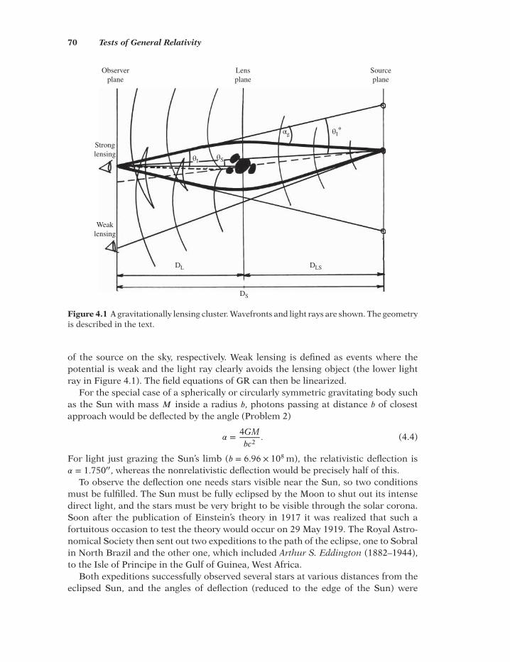
70 Tests of General Relativity
Observerplane
Stronglensing
Weaklensing
DS
DL DLS
θI θS
θI*αg
Lensplane
Sourceplane
Figure 4.1 A gravitationally lensing cluster. Wavefronts and light rays are shown. The geometryis described in the text.
of the source on the sky, respectively. Weak lensing is defined as events where thepotential is weak and the light ray clearly avoids the lensing object (the lower lightray in Figure 4.1). The field equations of GR can then be linearized.
For the special case of a spherically or circularly symmetric gravitating body suchas the Sun with mass 𝑀 inside a radius 𝑏, photons passing at distance 𝑏 of closestapproach would be deflected by the angle (Problem 2)
𝛼 = 4GM𝑏𝑐2
. (4.4)
For light just grazing the Sun’s limb (𝑏 = 6.96 × 10⁸ m), the relativistic deflection is𝛼 = 1.750′′, whereas the nonrelativistic deflection would be precisely half of this.
To observe the deflection one needs stars visible near the Sun, so two conditionsmust be fulfilled. The Sun must be fully eclipsed by the Moon to shut out its intensedirect light, and the stars must be very bright to be visible through the solar corona.Soon after the publication of Einstein’s theory in 1917 it was realized that such afortuitous occasion to test the theory would occur on 29 May 1919. The Royal Astro-nomical Society then sent out two expeditions to the path of the eclipse, one to Sobralin North Brazil and the other one, which included Arthur S. Eddington (1882–1944),to the Isle of Principe in the Gulf of Guinea, West Africa.
Both expeditions successfully observed several stars at various distances from theeclipsed Sun, and the angles of deflection (reduced to the edge of the Sun) were

Gravitational Lensing 71
1.98′′ ± 0.12′′ at Sobral and 1.61′′ ± 0.30′′ at Principe. This confirmed the predictedvalue of 1.750′′ with reasonable confidence and excluded the Newtonian value of0.875′′. The measurements have been repeated many times since then during latersolar eclipses, with superior results confirming the general relativistic prediction.
The case of starlight passing near the Sun is a special case of a general lensingevent, shown in Figure 4.1. For the Sun the distance from lens to observer is small sothat the angular size distances are 𝐷LS ≈ 𝐷S, which implies that the actual deflectionequals the observed deflection and 𝛼 = 𝜃I − 𝜃S. In the general case, simple geometrygives the relation between the deflection and the observed displacement as
𝛼 =𝐷S
𝐷LS(𝜃I − 𝜃S), (4.5)
For a lens composed of an ensemble of point masses, the deflection angle is, in thisapproximation, the vectorial sum of the deflections of the individual point lenses.When the light bending can be taken to be occurring instantaneously (over a shortdistance relative to 𝐷LS and 𝐷L), we have a geometrically thin lens, as assumed inFigure 4.1. Thick lenses are considerably more complicated to analyze.
Strong Lensing. The terms weak lensing and strong lensing are not defined veryprecisely. In weak lensing the deflection angles are small and it is relatively easyto determine the true positions of the lensed objects in the source plane from theirdisplaced positions in the observer plane. Strong lensing implies deflection throughlarger angles by stronger potentials. The images in the observer plane can then becomequite complicated because there may be more than one null geodesic connectingsource and observer, so that it is not even always possible to find a unique mappingonto the source plane. Strong lensing is a tool for testing the distribution of mass inthe lens rather than purely a tool for testing general relativity.
If a strongly lensing object can be treated as a point mass and is positioned exactlyon the straight line joining the observer and a spherical or pointlike lensed object, thelens focuses perfectly and the lensed image is a ring seen around the lens, called anEinstein ring. The angular size can be calculated by setting the two expressions for 𝛼,Equations (4.4) and (4.5), equal, noting that 𝜃S = 0 and solving for 𝜃I:
𝜃I =
√4GM𝐷LS
𝑐2𝐷L𝐷S. (4.6)
For small 𝑀 the image is just pointlike. In general, the lenses are galaxy clusters or(more rarely) single galaxies that are not spherical and the geometry is not simple, sothat the Einstein ring breaks up into an odd number of sections of arc. Each arc is acomplete but distorted picture of the lensed object.
In general, the solution of the lensing equation and the formation of multipleimages can be found by jointly solving Equations (4.4) and (4.5). Equation (4.4) givesthe bend angle 𝛼g(𝑀b) as a function of the gravitational potential for a (symmetric)mass 𝑀b within a sphere of radius 𝑏, or the mass seen in projection within a cir-cle of radius 𝑏. From Figure 4.1 we can see that 𝑏 = 𝜃I ×𝐷LS, so inserting this into

72 Tests of General Relativity
Equation (4.4) we have
𝛼g(𝑀b, 𝜃I) =4𝐺𝑀b
𝑐2𝜃I𝐷LS. (4.7)
Equation (4.5) is the fundamental lensing equation giving the geometrical relationbetween the bend angle 𝛼l and the source and image positions:
𝛼l(𝜃S, 𝜃I) =𝐷S
𝐷LS(𝜃I − 𝜃S). (4.8)
There will be an image at an angle 𝜃∗I that simultaneously solves both equations:
𝛼g(𝑀b, 𝜃∗I ) = 𝛼l(𝜃S, 𝜃
∗I ). (4.9)
For the case of a symmetric (or point-mass) lens, 𝜃∗I will be the two solutions to thequadratic
2𝜃∗𝐼= 𝜃S +
√𝜃
2S +
16𝐺𝑀b𝐷LS
𝑐2𝐷L𝐷S. (4.10)
This reduces to the radius of the Einstein ring when 𝜃S = 0. The angle correspondingto the radius of the Einstein ring we denote 𝜃E.
Equation (4.10) describes a pair of hyperbolas so there will always be two imagesfor a point-mass lens. When the source displacement is zero (𝜃S = 0) the images willbe at the positive and negative roots of Equation (4.6)—the Einstein ring. When 𝜃S islarge the positive root will be approximately equal to 𝜃S, while the negative root willbe close to zero (on the line of sight of the lens). This implies that every point-masslens should have images of every source, no matter what the separation in the sky.Clearly this is not the case. The reason is that the assumption of a point mass andhyperbolic 𝛼g cannot be maintained for small 𝜃I.
A more realistic assumption for the mass distribution of a galaxy would be thatthe density is spherically symmetric, with density as a function of distance from thegalactic core, 𝑅, given by
𝜌(𝑅) = 𝜌core
(1 + 𝑅2
𝑅2core
)−1
, (4.11)
The density is approximately constant (equal to 𝜌core) for small radii (𝑅 ≪ 𝑅core) andfalls off as 𝑅
−2 for large radii. This roughly matches observed mass-density distribu-tions (including dark matter) as inferred from galaxy rotational-velocity observations.The mass will grow like 𝑅
3 for 𝑅 ≪ 𝑅core and like 𝑅 for 𝑅 ≫ 𝑅core.For a nonsymmetric mass distribution, the function 𝛼g can become quite compli-
cated (see, e.g., [4]). Clearly, the problem quickly becomes complex. An example isshown in Figure 4.1, where each light ray from a lensed object propagates as a spher-ical wavefront. Bending around the lens then brings these wavefronts into positionsof interference and self-interaction, causing the observer to see multiple images. Thesize and shape of the images are therefore changed. From Figure 4.1 one understandshow the time delay of pairs of images arises: this is just the time elapsed between

Gravitational Lensing 73
different sheets of the same wavefront. In principle, the time delays in Equation (4.3)provides a tool for measuring 𝐻0.
Surface Brightness and Microlensing. Since photons are neither emitted norabsorbed in the process of gravitational light deflection, the surface brightness oflensed sources remains unchanged. Changing the size of the cross-section of a lightbundle therefore only changes the flux observed from a source and magnifies it atfixed surface-brightness level. For a large fraction of distant quasars the magnifica-tion is estimated to be a factor of ten or more. This enables objects of fainter intrinsicmagnitudes to be seen. However, lensing effects are very model dependent, so to learnthe true magnification effect one needs very detailed information on the structure ofthe lens.
If the mass of the lensing object is very small, one will merely observe a magnifi-cation of the brightness of the lensed object. This is called microlensing, and it hasbeen used to search for nonluminous objects in the halo of our Galaxy. One keepswatch over several million stars in the Large Magellanic Cloud (LMC) and recordsvariations in brightness. Some stars are Cepheids, which have an intrinsic variability,so they have to be discarded. A star which is small enough not to emit visible light andwhich is moving in the halo is expected to cross the diameter of a star in the LMC in atime span ranging from a few days to a couple of months. The total light amplificationfor all images from a point-mass lens and point source is (Problem 3)
𝐴 =1 + 1
2𝑥2
𝑥
√1 + 1
4𝑥2
, 𝑥 =𝜃S
𝜃E. (4.12)
As the relative positions of the source, lens and observer change, 𝜃S will change.Simple geometrical arguments give 𝜃S as a function of the relative velocities, and thusthe amplification as a function of time (see [4], pp. 106, 118–120). During the occul-tation, the image of the star behind increases in intensity according to this functionand subsequently decreases along the time-symmetric curve. A further requirementis that observations in different colors should give the same time curve. Several suchmicrolensing events have been found in the direction of the LMC, and several hun-dred in the direction of the bulge of our Galaxy. The number of such occurrences is,however, to small play any role as nonluminous dark matter later.
Cosmic Shear. The large-scale distribution of matter in the Universe is inhomoge-neous in every direction, so one can expect that everything we observe is displacedand distorted by weak lensing. Since the tidal gravitational field, and thus the deflec-tion angles, depend neither on the nature of the matter nor on its physical state, lightdeflection probes the total projected mass distribution. Lensing in infrared light offersthe additional advantage of sensing distant background galaxies, since their numberdensity is higher than in the optical. The idea of mapping the matter distribution usingthe cosmic shear field was already proposed (in 1937) by Fritz Zwicky (1898–1974),who also proposed looking for lensing by galaxies rather than by stars.

74 Tests of General Relativity
The ray-tracing process mapping a single source into its image can be expressedby the Jacobian matrix between the source-plane coordinates and the observer-planecoordinates:
J(𝛼) =(
1 − 𝜅 − 𝛾1 −𝛾2
−𝛾2 1 − 𝜅 + 𝛾1
), (4.13)
where 𝜅 is the convergence of the lens and 𝛾 = 𝛾1 + i𝛾2 is the shear. The matrix J(𝛼)transforms a circular source into an ellipse with semi-axes stretched by the factor(1 − 𝜅 ± |𝛾|)−1. The convergence affects the isotropic magnification or the projectedmass density divided by the critical density, whereas the shear affects the shape of theimage. The magnification is given by
𝜇 = (det J)−1 = [(1 − 𝜅)2 − 𝛾2]−1
. (4.14)
Clearly, there are locations where 𝜇 can become infinite. These points in the sourceplane are called caustics and they lie on the intersections of critical curves.
Weak Lensing Surveys. Background galaxies would be ideal tracers of distortionsif they were intrinsically circular. Any measured ellipticity would then directly reflectthe action of the gravitational tidal field of the interposed lensing matter, and thestatistical properties of the cosmic-shear field would reflect the statistical propertiesof the matter distribution. But many galaxies are actually intrinsically elliptical, andthe ellipses are randomly oriented. These intrinsic ellipticities introduce noise intothe inference of the tidal field from observed ellipticities.
The sky is covered with a ‘wall paper’ of faint and distant blue galaxies, about20 000–40 000 on an area of the size of the full moon. This fine-grained pattern ofthe sky makes statistical weak-lensing studies possible, because it allows the detec-tion of the coherent distortions imprinted by gravitational lensing on the images ofthe faint-blue-galaxy population. Large collaborations carrying out such surveys havereported statistically significant observations of cosmic shear and thus of the distri-bution of interposed lensing dark matter. We shall come back to this discussion in thechapter on dark matter.
To test general relativity versus alternative theories of gravitation, the best way is toprobe the gravitational potential far away from visible matter, and weak galaxy–galaxylensing being a good approach to this end because it is accurate on scales where allother methods fail, and it is simple if galaxies are treated as point masses. Alternativetheories may predict an isotropic signal where general relativity predicts an azimuthalvariation. The current knowledge favors anisotropy and thus general relativity.
4.4 Gravitational Waves
Einstein noted in 1916 that his general relativity predicted the existence of gravita-tional radiation, but its possible observation is still in the future. As we explained inSection 4.2, the slowdown of binary pulsars is indirect evidence that the system losesits energy by radiating gravitational waves.

Gravitational Waves 75
When gravitational waves travel through space-time they produce ripples of cur-vature, an oscillatory stretching and squeezing of space-time analogous to the tidaleffect of the Moon on Earth. Any matter they pass through will feel this effect. Thusa detector for gravitational waves is similar to a detector for the Moon’s tidal effect,but the waves act on an exceedingly weaker scale.
Gravitational radiation travels with the speed of light and traverses matter unhin-dered and unaltered. It may be that the carriers are particles, gravitons, with spin𝐽 = 2, but it is hard to understand how that could be verified. Perhaps, if a theorywere found combining gravitation and quantum mechanics, the particle nature ofgravitational radiation would be more meaningful.
Tensor Field. In contrast to the electromagnetic field, which is a vector field, thegravitational field is a tensor field. The gravitational analogue of electromagneticdipole radiation cannot produce any effect because of the conservation of momentum:any dipole radiation caused by the acceleration of an astronomical object is automat-ically cancelled by an equal and opposite change in momentum in nearby objects.Therefore, gravitational radiation is caused only by nonspherical symmetric accel-erations of mass, which can be related to the quadrupole moment, and the oscilla-tory stretch and squeeze produced is then described by two dimensionless wave fieldsℎ+ and ℎ×, which are associated with the gravitational wave’s two linear polarizations.If ℎ+ describes the amplitude of polarization with respect to the 𝑥- and 𝑦-axes in thehorizontal plane, ℎ× describes the independent amplitude of polarization with respectto the rotated axes 𝑥 + 𝑦 and 𝑥 − 𝑦 (see Figure 4.2). The relative tidal effect a detectorof length 𝐿 may observe is then a linear combination of the two wave fields
𝛥𝐿∕𝐿 = 𝑎+ℎ+(𝑡) + 𝑎×ℎ×(𝑡) ≡ ℎ(𝑡). (4.15)
The proper derivation of the quadrupole formula for the energy loss rate throughgravitational radiation of an oscillating body and the spatial strain ℎ(𝑡) caused onbodies elsewhere cannot be carried out here, it requires general relativity to be carriedout to high orders of covariant derivation. This complication is a benefit, however,because it renders the detection of gravitational radiation an extremely sensitive testof general relativity.
y y
z
x
+ polarization × polarization
x
z
Figure 4.2 The lines of force associated with the two polarizations of a gravitational wave.Reprinted with permission of A. Abramovici et al. [3]. Copyright 1992 American Associationfor the Advancement of Science.

76 Tests of General Relativity
In a Newtonian approximation the strength of the waves from a nonspherical bodyof mass 𝑀 , oscillating size 𝐿(𝑡), and quadrupole moment 𝑄(𝑡) ≈ 𝑀𝐿2 at a distance 𝑟
from Earth is
ℎ(𝑡) ≈ 𝐺
𝑐4𝑟
d2𝑄(𝑡)d𝑡2
= 𝐺
𝑐4𝑟2Mv(𝑡)2 = 4𝐺
𝑐4𝑟𝐸(𝑡), (4.16)
where 𝐺 is the Newtonian constant, 𝑣 is the internal velocity, and 𝐸 = 12𝑀𝑣2 is the
nonspherical part of the internal kinetic energy. The factor 𝑐4 is introduced only tomake ℎ(𝑡) dimensionless.
Sources of Gravitational Waves. From this formula one can work out that anonspherical symmetric supernova collapse at the center of our Galaxy will giverise to waves of amplitude ℎ ≈ 10−19 causing a subnuclear stretch and squeeze ofan object 1 km in length by 10−16 m. A spherically symmetric supernova collapsecauses no waves. In a catastrophic event such as the collision of two neutron starsor two stellar-mass black holes in which 𝐸∕𝑐2 is of the order of one solar mass,Equation (4.16) gives ℎ ≈ 10−20 at the 16 Mpc distance of the Virgo cluster of galaxies,and ℎ ≈ 10−21 at a distance of approximately 200 Mpc.
The signals one can expect to observe in the amplitude range ℎ ≈ 10−21–10−20 withthe present generation of detectors are bursts due to the coalescence of neutron-starbinaries during their final minutes and seconds (in the high frequency band 1–104 Hz),and periodic waves from slowly merging galactic binaries and extragalactic mas-sive black hole binaries (low-frequency band 10−4–10−2 Hz), which are stable overhundreds to millions of years. The timing of millisecond binary pulsars such as thePSR 1913 + 16 belong to the very low-frequency band of 10−9–10−7 Hz. In this band,processes in the very early Universe may also act as sources.
Merger waves from superheavy black holes with 106𝑀⊙
mass may be so strong thatboth their direction and their amplitude can be determined by monitoring the waveswhile the detector rotates around the Sun. This may permit researchers to identifythe source with the parallax method and to determine the distance to it with highprecision. Combined with redshift measurements of the source, one could determinenot only 𝐻0 but even the deceleration parameter 𝑞0 of the Universe. Thus the detectionof gravitational waves from black holes would go beyond testing general relativity todetermining fundamental cosmological parameters of the Universe.
The dynamics of a hole–hole binary can be divided into three epochs: inspiral,merger and ringdown. The inspiral epoch ends when the holes reach their last sta-ble orbit and begin plunging toward each other. Then the merger epoch commences,during which the binary is a single nonspherical black hole undergoing highly nonlin-ear space-time oscillations and vibrations of large amplitude. In the ringdown epoch,the oscillations decay due to gravitational wave emission, leaving finally a spherical,spinning black hole.
Gravitational Wave Detection. Detection with huge metal bars as resonant anten-nas was started by Joseph Weber in 1969. These detectors couple to one axis of the

Gravitational Waves 77
L2
L2
Mirror
Mirrors
Laser
Photodiode
Beamsplitter
R Mirror
Figure 4.3 A schematic view of a LIGO-type interferometer. Reprinted with permission ofA. Abramovici et al. [3]. Copyright 1992 American Association for the Advancement of Science.
eigenmodes of the incoming wave, and one then expects to observe a change in thestate of oscillation. Today several coordinated and aligned cryogenic bar detectors arein coordinated operation with sensitivities of approximately 10−21 Hz−1∕2. The detec-tors are tuned to see approximately 1 ms bursts occurring within a bandwidth of theorder of 1 Hz. In order to eliminate random noise, the data from several detectors areanalyzed for coincidences.
To improve the signal to noise ratio in the high-frequency range one turnsto Michelson interferometers with very long arms. The principle is illustrated inFigure 4.3. A laser beam is split, travels in two orthogonal directions to mirrors, andreturns to be recombined and detected. A gravitational wave with either the ℎ+ orℎ× component coinciding with the interferometer axes would lengthen the round-tripdistance to one mirror and shorten it to the other. This would be observable as a mis-match of waves upon recombination, and hence as a decrease in the observed com-bined intensity of the laser. For isolation against mechanical disturbances the opticalcomponents are carefully suspended in vacuum. The arm lengths in active terrestrialdetectors range from 300 m (TAMA in Japan) and 600 m (GEO600 in Germany) to 3 km(VIRGO in Italy) and 4 km (LIGO at two locations in the United States). Sensitivitiesof 10−21–10−22 Hz−1∕2 can be reached in the high-frequency range. The range is limitedto less than approximately 104 Hz by photo-electron shot noise in the components ofthe interferometer.
To study sources in the low-frequency range one has to put the interferometer intospace orbiting Earth. This is necessary in order to avoid low-frequency seismic noiseon the ground and thermally induced medium-frequency motion in the atmosphere.The spectacular solution is the detector LISA (Laser Interferometer Space Antenna)consisting of three identical spacecraft, forming an equilateral triangle in space, withsidelength 5 million km, trailing Earth by 20∘ in a heliocentric orbit (see Figure 4.4).From each spacecraft a 1 W beam is sent to the two other remote spacecrafts via atelescope, is reflected by a platinum–gold cubic test mass, and the same telescopesare then used to focus the very weak returning beams. The interference signals

78 Tests of General Relativity
Earth
1 AU
Sun
1 × 10⁹ m
60°
20°
Figure 4.4 eLISA orbits in the Solar System [4]. Reproduced with permission of Pau Amaro-Seoane and the LISA consortium. (See plate section for color version.)
from each arm are combined by on-board computers to perform the multiple-arminterferometry required to cancel the phase-noise common to all three arms. Fluctu-ations in the optical paths between the test masses can be measured to sub-angstromprecision, which, when combined with the large separation of the spacecraft, allowedLISA to detect gravitational-wave strain down to a level of order 10−23 in one year ofobservation, with a signal to noise ratio of 5.
LISA targets high-priority astronomy such as massive black holes, stellar evolution,the high-redshift universe and cosmology. By 2011 LISA had identified 20 000 individ-ual sources, almost all resolvable binary white dwarfs, but no black hole—black holemergers and no signals of gravitational radiation [4]. Its follower, the European-ledvariant named eLISA (see Figure 4.4 [4]) is scheduled to be launched before 2022.
Problems
1. Calculate the gravitational redshift in wavelength for the 769.9 nm potassiumline emitted from the Sun’s surface [1].
2. Derive the deflection angle [Equation (4.4)] using Equations (4.26) and (4.5).
3. Derive Equation (4.12). What are the amplification of the individual images [4]?
4. Draw the bend angle due to gravitational potential 𝛼g and lens geometry 𝛼l, andzero (dashed line) for a lens of mass 𝑀 ≈ 7.2 × 10¹¹𝑀
⊙, with 𝐷S ≈ 1.64 Gpc (𝑧 =
3.4 in a FRW cosmology with 𝛺m = 0.3 and 𝛺𝜆= 0.7), 𝐷L ≈ 1.67 Gpc (𝑧 = 0.803),
𝐷LS ≈ 0.96 Gpc and 𝛼S ≈ 0.13′′. (Note that since distances are angular diameterdistances, 𝐷S ≠ 𝐷LS +𝐷L.) Take the lens to be (a) a point mass and (b) a spher-ical mass distribution with density given by Equation (4.11) for an ideal galaxy.This roughly corresponds to the parameters associated with the ‘Einstein Cross’lensed quasar found by the Hubble telescope, HST 14176 + 5226.

Gravitational Waves 79
References[1] Kenyon, I. R. 1990 General relativity. Oxford University Press, Oxford.[2] Will, C. M. 1993 Theory and experiment in gravitational physics, revised edn. Cambridge
University Press, Cambridge.[3] Abramovici, A. et al. 1992 Science 256, 325.[4] Amaro-Seoane, P. et al. 2013 G.W. Notes 6, 4–110.


5
Cosmological Models
In Section 5.1 we turn to the ‘concordance’ or Friedmann–Lemaitre–Robertson–Walker (FLRW) model of cosmology, really only a paradigm based on Friedmann’sand Lemaitre’s equations and the Robertson–Walker metric, which takes both energydensity and pressure to be functions of time in a Copernican universe. Among thesolutions are the Einstein universe and the Einstein–de Sitter universe, both nowknown to be wrong, as we shall see in Section 5.4, and the currently acceptedFriedmann–Lemaitre universe, which includes a positive cosmological constant.
In Section 5.2 we describe the de Sitter model, which does not apply to the Universeat large as we see it now, but which may have dominated the very early universe, andwhich may be the correct description for the future.
In Section 5.3 we introduce tne Schwartzschild solution to The Einstein equation.This takes us to black holes in Section 5.4.
In Section 5.5 we briefly present extensions of general relativity.
5.1 Friedmann–Lemaitre Cosmologies
Let us now turn to our main subject, a model describing our homogeneous andisotropic Universe for which the Robertson–Walker metric in Equation (2.32) wasderived. Recall that it could be written as a 4 × 4 tensor with nonvanishing com-ponents [Equation (2.33)] on the diagonal only, and that it contained the curvatureparameter 𝑘.
Friedmann’s Equations. The stress–energy tensor 𝑇𝜇𝜈
entering on the right-handside of the Einstein Equations (3.29) was given by Equation (3.30) in its diagonalform. For a comoving observer with velocity four-vector 𝑣 = (𝑐,0,0,0), the time–time
Introduction to Cosmology, Fourth Edition. Matts Roos© 2015 John Wiley & Sons, Ltd. Published 2015 by John Wiley & Sons, Ltd.
82 Cosmological Models
component 𝑇00 and the space–space component 𝑇11 are then
𝑇00 = 𝜌𝑐2, 𝑇11 = 𝑝𝑎
2
1 − 𝑘𝜎2, (5.1)
taking 𝑔00 and 𝑔11 from Equation (2.33). We will not need 𝑇22 or 𝑇33 because they justduplicate the results without adding new dynamical information. In what follows weshall denote mass density by 𝜌 and energy density by 𝜌𝑐2. Occasionally, we shall use𝜌m𝑐
2 to denote specifically the energy density in all kinds of matter: baryonic, leptonicand unspecified dark matter. Similarly we use 𝜌r𝑐
2 or 𝜀 to specify the energy densityin radiation.
On the left-hand side of the Einstein Equations (3.29) we need𝐺00 and𝐺11 to equatewith 𝑇00 and 𝑇11, respectively. We have all the tools to do it: the metric components 𝑔
𝜇𝜈
are inserted into Equation (3.13) for the affine connection, and subsequently we calcu-late the components of the Riemann tensor from the expression (3.16) using the metriccomponents and the affine connections. This lets us find the Ricci tensor componentsthat we need, 𝑅00 and 𝑅11, and the Ricci scalar from Equations (3.17) and (3.18),respectively. All this would require several pages to work out (see, e.g., [1, 2]), so I onlygive the result:
𝐺00 = 3(ca)−2 (��
2 + 𝑘𝑐2), (5.2)
𝐺11 = −𝑐−2 (2𝑎�� + ��2 + 𝑘𝑐2) (1 − 𝑘𝜎2)−1. (5.3)
Here 𝑎 is the cosmic scale factor 𝑎(𝑡) at time 𝑡. Substituting Equations (4.1)–(4.3) intothe Einstein Equations (3.29) we obtain two distinct dynamical relations for 𝑎(𝑡):
��2 + 𝑘𝑐2
𝑎2= 8𝜋𝐺
3𝜌, (5.4)
2��𝑎
+ ��2 + 𝑘𝑐2
𝑎2= −8𝜋𝐺
𝑐2𝑝. (5.5)
These equations were derived in 1922 by Friedmann, seven years before Hubble’sdiscovery, at a time when even Einstein did not believe in his own equations becausethey did not allow the Universe to be static. Friedmann’s equations did not gain gen-eral recognition until after his death, when they were confirmed by an independentderivation (in 1927) by Georges Lemaitre (1894–1966). For now they will constitutethe tools for our further investigations.
The expansion (or contraction) of the Universe is inherent to Friedmann’s equa-tions. Equation (5.4) shows that the rate of expansion, ��, increases with the mass den-sity 𝜌 in the Universe, and Equation (5.5) shows that it may accelerate. SubtractingEquation (5.4) from Equation (5.5) we obtain
2��𝑎
= −8𝜋𝐺3𝑐2
(𝜌𝑐2 + 3𝑝), (5.6)
which shows that the acceleration decreases with increasing pressure and energy den-sity, whether mass or radiation energy. Thus it is more appropriate to talk about thedeceleration of the expansion. Equation 5.6 is also called the Raychauduri equation.

Friedmann–Lemaitre Cosmologies 83
At our present time 𝑡0 when the mass density is 𝜌0, the cosmic scale is 1, the Hub-ble parameter is 𝐻0 and the density parameter 𝛺0 is given by Equation (1.35), Fried-mann’s equation (5.4) takes the form
��20 = 8
3𝜋𝐺𝜌0 − 𝑘𝑐2 = 𝐻2
0𝛺0 − 𝑘𝑐2, (5.7)
which can be rearranged as
𝑘𝑐2 = 𝐻2
0 (𝛺0 − 1). (5.8)
It is interesting to note that this reduces to the Newtonian relation (1.35). Thus therelation between the Robertson–Walker curvature parameter 𝑘 and the present densityparameter𝛺0 emerges: to the 𝑘 values +1, 0 and −1 correspond an overcritical density𝛺0 > 1, a critical density 𝛺0 = 1 and an undercritical density 0 < 𝛺0 < 1, respectively.The spatially flat case with 𝑘 = 0 is called the Einstein–de Sitter universe.
General Solution. When we generalized from the present𝐻0 to the time-dependentHubble parameter𝐻(𝑡) = ��∕𝑎 in Equation (2.47), this also implied that the critical den-sity [Equation (1.31)] and the density parameter [Equation (1.35)] became functionsof time:
𝜌c(𝑡) =3
8𝜋𝐺𝐻
2(𝑡), (5.9)
𝛺(𝑡) = 𝜌(𝑡)∕𝜌c(𝑡). (5.10)
Correspondingly, Equation (5.8) can be generalized to
𝑘𝑐2 = 𝐻2
𝑎2(𝛺 − 1). (5.11)
If 𝑘 ≠ 0, we can eliminate 𝑘𝑐2 between Equations (5.8) and (5.11) to obtain
𝐻2𝑎
2(𝛺 − 1) = 𝐻20 (𝛺0 − 1), (5.12)
which we shall make use of later.It is straightforward to derive a general expression for the solution of Friedmann’s
Equation (5.4). Inserting 𝑘𝑐2 from Equation (5.8), and replacing (8𝜋𝐺∕3)𝜌 by 𝛺(𝑎)𝐻20 ,
Equation (5.4) furnishes a solution for 𝐻(𝑎):
𝐻(𝑎) ≡ ��∕𝑎 = 𝐻0
√(1 −𝛺0)𝑎−2 +𝛺(𝑎). (5.13)
Here we have left the 𝑎 dependence of 𝛺(𝑎) unspecified. As we shall see later, varioustypes of energy densities with different 𝑎 dependences contribute.
Equation (5.13) can be used to solve for the lookback time 𝑡(𝑧)∕𝑡0 or 𝑡(𝑎)∕𝑡0 (nor-malized to the age 𝑡0) since a photon with redshift 𝑧 was emitted by writing it as anintegral equation:
∫
𝑡(𝑎)
0d𝑡 =
∫
𝑎
1
d𝑎aH(𝑎)
. (5.14)
The age of the Universe at a given redshift is then 1 − 𝑡(𝑧)∕𝑡0. We shall specify this inmore detail later.

84 Cosmological Models
Einstein Universe. Consider now the static universe cherished by Einstein. This isdefined by 𝑎(𝑡) being constant, 𝑎(𝑡0) = 1, so that �� = 0 and �� = 0 and the age of theUniverse is infinite. Equations (5.4) and (5.5) then reduce to
𝑘𝑐2 = 8𝜋
3𝐺𝜌0 = −8𝜋
𝑐2𝐺𝑝0. (5.15)
In order that the mass density 𝜌0 be positive today, 𝑘 must be +1. Note that this leadsto the surprising result that the pressure of matter 𝑝0 becomes negative!
Einstein corrected for this in 1917 by introducing a constant Lorentz-invariantterm 𝜆𝑔
𝜇𝜈into Equation (3.28), where the cosmological constant 𝛺
𝜆corresponds to
a tiny correction to the geometry of the Universe. Equation (3.28) then becomes
𝐺𝜇𝜈
= 𝑅𝜇𝜈
− 12𝑔𝜇𝜈𝑅 − 𝜆𝑔
𝜇𝜈. (5.16)
In contrast to the first two terms on the right-hand side, the 𝜆𝑔𝜇𝜈
term does notvanish in the limit of flat space-time. With this addition, Friedmann’s equations takethe form
��2 + 𝑘𝑐2
𝑎2− 𝜆
3= 8𝜋𝐺
3𝜌, (5.17)
2��𝑎
+ ��2 + 𝑘𝑐2
𝑎2− 𝜆 = −8𝜋𝐺
𝑐2𝑝. (5.18)
A positive value of 𝜆 curves space-time so as to counteract the attractive gravitationof matter. Einstein adjusted 𝜆 to give a static solution, which is called the Einsteinuniverse.
The pressure of matter is certainly very small, otherwise one would observe thegalaxies having random motion similar to that of molecules in a gas under pressure.Thus one can set 𝑝 = 0 to a good approximation. In the static case when 𝑎 = 1, ��0 = 0and ��0 = 0, Equation (5.17) becomes
𝑘𝑐2 − 𝜆
3= 8𝜋𝐺
3𝜌0.
It follows from this that in a spatially flat Universe
𝜌𝜆= 𝜆
8𝜋𝐺= −𝜌0. (5.19)
But Einstein did not notice that the static solution is unstable: the smallest imbal-ance between 𝜆 and 𝜌 would make �� nonzero, causing the Universe to accelerate intoexpansion or decelerate into contraction. This flaw was only noticed by Eddington in1930, soon after Hubble’s discovery, in 1929, of the expansion that caused Einsteinto abandon his belief in a static universe and to withdraw the cosmological constant.This he called ‘the greatest blunder of my lifetime’.
The Friedmann–Lemaitre Universe. If the physics of the vacuum looks the sameto any inertial observer, its contribution to the stress–energy tensor is the same asEinstein’s cosmological constant 𝜆, as was noted by Lemaitre. The 𝜆 term in Equa-tion (5.16) is a correction to the geometrical terms in 𝐺
𝜇𝜈, but the mathematical con-
tent of Equations (5.17) and (5.18) are not changed if the 𝜆 terms are moved to the

Friedmann–Lemaitre Cosmologies 85
right-hand side, where they appear as corrections to the stress–energy tensor 𝑇𝜇𝜈
. Thenthe physical interpretation is that of an ideal fluid with energy density 𝜌
𝜆= 𝜆∕8𝜋𝐺 and
negative pressure 𝑝𝜆= −𝜌
𝜆𝑐2. When the cosmological constant is positive, the gravita-
tional effect of this fluid is a cosmic repulsion counteracting the attractive gravitationof matter, whereas a negative 𝜆 corresponds to additional attractive gravitation.
The cosmology described by Equations (5.17) and (5.18) with a positive cosmolog-ical constant is called the Friedmann–Lemaitre universe or the Concordance model.Such a universe is now strongly supported by observations of a nonvanishing 𝜆, sothe Einstein–de Sitter universe, which has 𝜆 = 0, is a dead end.
In a Friedmann–Lemaitre universe the total density parameter is conveniently splitinto a matter term, a radiation term and a cosmological constant term,
𝛺0 = 𝛺m +𝛺r +𝛺𝜆, (5.20)
where 𝛺r and 𝛺𝜆
are defined analogously to Equations (1.35) and (5.10) as
𝛺r =𝜌r
𝜌c, 𝛺
𝜆= 𝜆
8𝜋𝐺𝜌c= 𝜆
3𝐻20
. (5.21)
𝛺m, 𝛺r and 𝛺𝜆
are important dynamical parameters characterizing the Universe. Ifthere is a remainder 𝛺
𝑘≡ 𝛺0 − 1 ≠ 0, this is called the vacuum-energy term.
Using Equation (5.19) we can find the value of 𝜆 corresponding to the attractivegravitation of the present mass density:
−𝜆 = 8𝜋𝐺𝜌0 = 3𝛺0𝐻20 ≈ 1.3 × 10−52
𝑐2 m−2
. (5.22)
No quantity in physics this small has ever been known before. It is extremelyuncomfortable that 𝜆 has to be fine-tuned to a value which differs from zero onlyin the 52nd decimal place (in units of 𝑐 = 1). It would be much more natural if 𝜆 wereexactly zero. This situation is one of the enigmas which will remain with us to theend of this book. As we shall see, a repulsive gravitation of this kind may have been ofgreat importance during the first brief moments of the existence of the Universe, andit appears that the present Universe is again dominated by a global repulsion.
Energy-Momentum Conservation. Let us study the solutions of Friedmann’s equa-tions in the general case of nonvanishing pressure 𝑝. Differentiating Equation (5.4)with respect to time,
dd𝑡
(��2 + 𝑘𝑐2) = 8𝜋𝐺3
dd𝑡
(𝜌𝑎2),
we obtain an equation of second order in the time derivative:
2���� = 83𝜋𝐺(��𝑎2 + 2𝜌𝑎��). (5.23)
Using Equation (5.6) to cancel the second-order time derivative and multiplyingthrough by 𝑐2∕𝑎2, we obtain a new equation containing only first-order time deriva-tives:
��𝑐2 + 3𝐻(𝜌𝑐2 + 𝑝) = 0. (5.24)

86 Cosmological Models
This equation does not contain 𝑘 and 𝜆, but that is not a consequence of having startedfrom Equations (5.4) and (5.5). If, instead, we had started from Equations (5.17)and (5.18), we would have obtained the same equation.
Note that all terms here have dimension of energy density per time. In other words,Equation (5.24) states that the change of energy density per time is zero, so we caninterpret it as the local energy conservation law. In a volume element d𝑉 , 𝜌𝑐2 d𝑉 rep-resents the local decrease of gravitating energy due to the expansion, whereas 𝑝 d𝑉 isthe work done by the expansion. Energy does not have a global meaning in the curvedspacetime of general relativity, whereas work does. If different forms of energy do nottransform into one another, each form obeys Equation (5.24) separately. The Einsteinequation needs to be extended in some way to be able to serve as a global energy con-servation law. There is no “correct” way to do it, but many suggestions. We shall notpursue that search here.
As we have seen, Equation (5.24) follows directly from Friedmann’s equations with-out any further assumptions. But it can also be derived in another way, perhaps moretransparently. Let the total energy content in a comoving volume 𝑎3 be
𝐸 = (𝜌𝑐2 + 𝑝)𝑎3.
The expansion is adiabatic if there is no net inflow or outflow of energy so that
d𝐸d𝑡
= dd𝑡
[(𝜌𝑐2 + 𝑝)𝑎3] = 0. (5.25)
If 𝑝 does not vary with time, changes in 𝜌 and 𝑎 compensate and Equation (5.24)immediately follows.
Equation (5.24) can easily be integrated,
∫
��(𝑡)𝑐2
𝜌(𝑡)𝑐2 + 𝑝(𝑡)d𝑡 = −3
∫
��(𝑡)𝑎(𝑡)
d𝑡, (5.26)
if we know the relation between energy density and pressure—the equation of state ofthe Universe.
Entropy Conservation and the Equation of State. In contrast, the law of conser-vation of entropy 𝑆 is not implied by Friedmann’s equations, it has to be assumedspecifically, as we shall demonstrate in Section 5.2,
�� = 0. (5.27)
Then we can make an ansatz for the equation of state: let 𝑝 be proportional to 𝜌𝑐2 withsome proportionality factor 𝑤 which is a constant in time,
𝑝 = 𝑤𝜌𝑐2. (5.28)
Inserting this ansatz into the integral in Equation (5.26) we find that the relationbetween energy density and scale is
𝜌(𝑎) ∝ 𝑎−3(1+𝑤) = (1 + 𝑧)3(1+𝑤). (5.29)
Here we use 𝑧 as well as 𝑎 because astronomers prefer 𝑧 since it is an observable. Incosmology, however, it is better to use 𝑎 for two reasons. Firstly, redshift is a property

Friedmann–Lemaitre Cosmologies 87
of light, but freely propagating light did not exist at times when 𝑧 ≳ 1080, so 𝑧 is thenno longer a true observable. Secondly, it is possible to describe the future in terms of𝑎 > 1, but redshift is then not meaningful.
The value of the proportionality factor 𝑤 in Equations (5.28) and (5.29) followsfrom the adiabaticity condition. Leaving the derivation of 𝑤 for a later discussion, weshall anticipate here its value in three special cases of great importance.
Case I. A matter-dominated universe filled with nonrelativistic cold matter in theform of pressureless nonradiating dust for which 𝑝 = 0. From Equation 5.28then, this corresponds to 𝑤 = 0, and the density evolves according to
𝜌m(𝑎) ∝ 𝑎−3 = (1 + 𝑧)3. (5.30)
It follows that the evolution of the density parameter 𝛺m is
𝛺m(𝑎) = 𝛺m
𝐻20
𝐻2𝑎−3.
Solving for 𝐻2𝑎2𝛺 and inserting it into Equation (5.13), one finds the evo-lution of the Hubble parameter:
𝐻(𝑎) = 𝐻0𝑎−1√
1 −𝛺m +𝛺m𝑎−1 = 𝐻0(1 + 𝑧)
√1 +𝛺m𝑧. (5.31)
Case II. A radiation-dominated universe filled with an ultra-relativistic hot gas com-posed of elastically scattering particles of energy density 𝜀. Statisticalmechanics then tells us that the equation of state is
𝑝r =13𝜀 = 1
3𝜌r𝑐
2. (5.32)
This evidently corresponds to 𝑤 = 13, so that the radiation density evolves
according to
𝜌r(𝑎) ∝ 𝑎−4 = (1 + 𝑧)4. (5.33)
Case III. The vacuum-energy state corresponds to a flat, static universe (�� = 0, �� =0) without dust or radiation, but with a cosmological term. From Equa-tions (5.17) and (5.18) we then obtain
𝑝𝜆= −𝜌
𝜆𝑐
2, 𝑤 = −1. (5.34)
Thus the pressure of the vacuum energy is negative, in agreement withthe definition in Equation (5.19) of the vacuum-energy density as a nega-tive quantity. In the equation of state [Equation (5.28)], 𝜌
𝜆and 𝑝
𝜆are then
scale-independent constants.
Early Time Dependence. It follows from the above scale dependences that thecurvature term in Equation (5.17) obeys the following inequality in the limit ofsmall 𝑎:
𝑘𝑐2
𝑎2≪
8𝜋𝐺3𝜌 + 𝜆
3. (5.35)

88 Cosmological Models
In fact, this inequality is always true when
𝑘 = +1, 𝑝 > −13𝜌𝑐
2, 𝑤 > −1
3, 𝜆 > 0. (5.36)
Then we can neglect the curvature term and the 𝜆 term in Equation (5.17), whichsimplifies to
��
𝑎= 𝐻(𝑡) =
(8𝜋𝐺
3𝜌
)1∕2
∝ 𝑎−3(1+𝑤)∕2. (5.37)
Let us now find the time dependence of 𝑎 by integrating this differential equation:
∫d𝑎 𝑎−1+3(1+𝑤)∕2 ∝
∫d𝑡,
to obtain the solutions
𝑎3(1+𝑤)∕2 ∝ 𝑡 for 𝑤 ≠ −1, ln 𝑎 ∝ 𝑡 for 𝑤 = −1.
Solving for 𝑎,
𝑎(𝑡) ∝ 𝑡2∕3(1+𝑤) for 𝑤 ≠ −1, 𝑎(𝑡) ∝ econst.⋅𝑡 for 𝑤 = −1. (5.38)
In the two epochs of matter domination and radiation domination we know thevalue of 𝑤. Inserting this we obtain the time dependence of 𝑎 for a matter-dominateduniverse,
𝑎(𝑡) ∝ 𝑡2∕3, (5.39)
and for a radiation-dominated universe,
𝑎(𝑡) ∝ 𝑡1∕2. (5.40)
Big Bang. We find the starting value of the scale of the Universe independently ofthe value of 𝑘 in the curvature term neglected above:
lim𝑡→0𝑎(𝑡) = 0. (5.41)
In the same limit the rate of change �� is obtained from Equation (5.37) with any 𝑤obeying 𝑤 > −1:
lim𝑡→0��(𝑡) = lim
𝑡→0𝑎−1(𝑡) = ∞. (5.42)
It follows from Equations (5.32) and (5.33) that an early radiation-dominated Uni-verse was characterized by extreme density and pressure:
lim𝑡→0𝜌r(𝑡) = lim
𝑡→0𝑎−4(𝑡) = ∞,
lim𝑡→0𝑝r(𝑡) = lim
𝑡→0𝑎−4(𝑡) = ∞.
In fact, these limits also hold for any 𝑤 obeying 𝑤 > −1.Actually, we do not even need an equation of state to arrive at these limits. Pro-
vided 𝜌𝑐2 + 3𝑝 was always positive and 𝜆 negligible, we can see from Equations (5.6)

Friedmann–Lemaitre Cosmologies 89
and (5.18) that the Universe has always decelerated. It then follows that 𝑎 must havebeen zero at some time in the past. Whether Friedmann’s equations can in fact betrusted to that limit is another story which we shall come back to later. The time 𝑡 = 0was sarcastically called the Big Bang by Fred Hoyle, who did not like the idea of anexpanding Universe starting from a singularity, but the name has stuck. Since about1988 the steady state theory has been abandoned because of the discovery of earlyquasars.
Late Einstein–de Sitter Evolution. The conclusions we derived from Equation(5.35) were true for past times in the limit of small 𝑎. However, the recent evolutionand the future depend on the value of 𝑘 and on the value of 𝜆. For 𝑘 = 0 and 𝑘 = −1the expansion always continues, following Equation (5.38), and a positive value of 𝜆boosts the expansion further.
In a matter-dominated Einstein–de Sitter universe which is flat and has 𝛺𝜆= 0,
Friedmann’s Equation (5.4) can be integrated to give
𝑡(𝑧) = 23𝐻0
(1 + 𝑧)−3∕2, (5.43)
and the present age of the Universe at 𝑧 = 0 would be
𝑡0 = 23𝐻0
. (5.44)
In that case the size of the Universe would be 𝑐𝑡0 = 2ℎ−1 Gpc. Inserting the value of𝐻0
used in Equation (1.21), 𝐻0 = 0.696 km s−1 Mpc−1, one finds
𝑡0 = 9.27 Gyr. (5.45)
This is in obvious conflict with 𝑡0 as determined from the ages of the oldest knownstar in the Galaxy in Equation (1.24), 13.5 ± 2.9 Gyr. Thus the flat-universe model with𝛺𝜆= 0 is in trouble.
Evolution of a Closed Universe. In a closed matter-dominated universe with 𝑘 =+1 and 𝜆 = 0, the curvature term 𝑘𝑐
2∕𝑎2 drops with the second power of 𝑎, while,according to Equation (5.30), the density drops with the third power, so the inequality[Equation (5.35)] is finally violated. This happens at a scale 𝑎max such that
𝑎−2max =
8𝜋𝐺𝜌m
3𝑐2, (5.46)
and the expansion halts because �� = 0 in Equation (5.4). Let us call this the turnovertime 𝑡max. At later times the expansion turns into contraction, and the Universe returnsto zero size at time 2𝑡max. That time is usually called the Big Crunch. For 𝑘 = +1 Fried-mann’s Equation (5.4) then takes the form
d𝑎d𝑡
=√
8𝜋3𝐺𝜌m(𝑎)𝑎2 − 𝑐2.

90 Cosmological Models
Then 𝑡max is obtained by integrating 𝑡 from 0 to 𝑡max and 𝑎 from 0 to max,
𝑡max = 1𝑐 ∫
𝑎max
0d𝑎
(8𝜋𝐺3𝑐2
𝜌m(𝑎)𝑎2 − 1)−1∕2
. (5.47)
To solve the 𝑎 integral we need to know the energy density 𝜌m(𝑎) in terms of thescale factor, and we need to know 𝑎max. Let us take the mass of the Universe to be 𝑀 .We have already found in Equation (2.43) that the volume of a closed universe withRobertson–Walker metric is
𝑉 = 2𝜋2𝑎
3.
Since the energy density in a matter-dominated universe is mostly pressurelessdust,
𝜌m = 𝑀
𝑉= 𝑀
2𝜋2𝑎3. (5.48)
This agrees perfectly with the result [Equation (5.30)] that the density is inverselyproportional to 𝑎3. Obviously, the missing proportionality factor in Equation (5.30) isthen𝑀∕2𝜋2. Inserting the density [Equation (5.48)] with 𝑎 = 𝑎max into Equation (5.46)we obtain
𝑎max = 4MG3𝜋𝑐2
. (5.49)
We can now complete the integral in Equation (5.47):
𝑡max = 𝜋
2𝑐𝑎max = 2MG
3𝑐3. (5.50)
Although we might not know whether we live in a closed universe, we certainlyknow from the ongoing expansion that 𝑡max > 𝑡0. Using the value for 𝑡0 from Equa-tion (1.21) we find a lower limit to the mass of the Universe:
𝑀 >3𝑡0𝑐
3
2𝐺= 1.30 × 10²³
𝑀⊙. (5.51)
Actually, the total mass inside the present horizon is estimated to be about 1022𝑀⊙
.The dependence of 𝑡max on 𝛺m can also be obtained:
𝑡max =𝜋𝛺m
2𝐻0(𝛺m − 1)3∕2. (5.52)
The three cases 𝑘 = −1, 0, +1 with 𝜆 = 0 are illustrated qualitatively in Figure 5.1.All models have to be consistent with the scale and rate of expansion today, 𝑎 = 1 and��0, at time 𝑡0. Following the curves back in time one notices that they intersect thetime axis at different times. Thus what may be called time 𝑡 = 0 is more recent in aflat universe than in an open universe, and in a closed universe it is even more recent.
The Radius of the Universe. The spatial curvature is given by the Ricci scalar 𝑅introduced in Equation (3.18), and it can be expressed in terms of 𝛺:
𝑅 = 6𝐻2(𝛺 − 1). (5.53)

Friedmann–Lemaitre Cosmologies 91
R(t) de Sitter
H cons
tant k = –1
k = 0
future
0
–1
+1
tmax t
tH
to
past
k =
tH23
Figure 5.1 Time dependence of the cosmic scale 𝑅(𝑡) = 𝑎(𝑡) in various scenarios, all of whichcorrespond to the same constant slope𝐻 = 𝐻0 at the present time 𝑡0. 𝑘 = +1: a closed universewith a total lifetime 2𝑡max. It started more recently than a flat universe would have. 𝑘 = 0: a flat
universe which started 23𝑡H ago. 𝑘 = −1: an open universe which started at a time 2
3𝑡H < 𝑡 < 𝑡H
before the present time. de Sitter: an exponential (inflationary) scenario corresponding to alarge cosmological constant. This is also called the Lemaitre cosmology.
Obviously, 𝑅 vanishes in a flat universe, and it is only meaningful when it is non-negative, as in a closed universe. It is conventional to define a ‘radius of curvature’that is also valid for open universes:
𝑟U ≡
√6𝑅
= 1
𝐻
√|𝛺 − 1| . (5.54)
For a closed universe, 𝑟U has the physical meaning of the radius of a sphere.
Late Friedmann–Lemaitre Evolution. When 𝜆 > 0, the recent past and the futuretake an entirely different course (we do not consider the case 𝜆 < 0, which is of mathe-matical interest only). Since 𝜌
𝜆and𝛺
𝜆are then scale-independent constants, they will
start to dominate over the matter term and the radiation term when the expansion hasreached a given scale. Friedmann’s Equation (5.18) can then be written
2��𝑎
= 3𝐻20𝛺𝜆.
From this one sees that the expansion will accelerate regardless of the value of 𝑘. Inparticular, a closed universe with 𝑘 = +1 will ultimately not contract, but expand atan accelerating pace.

92 Cosmological Models
Let us now return to the general expression [Equation (5.14)] for the normalizedage 𝑡(𝑧)∕𝑡0 or 𝑡(𝑎)∕𝑡0 of a universe characterized by 𝑘 and energy density components𝛺m, 𝛺r and 𝛺
𝜆. Inserting the 𝛺 components into Equations (5.13) and (5.14) we have
��2
𝑎2= 𝐻2(𝑡) = 𝐻2
0 [(1 −𝛺0)𝑎−2 +𝛺m(𝑎) +𝛺r(𝑎) +𝛺𝜆(𝑎)],
or
𝑡(𝑧) = 1𝐻0 ∫
1∕(1+𝑧)
0d𝑎 [(1 −𝛺0) +𝛺m𝑎
−1 +𝛺r𝑎−2 +𝛺
𝜆𝑎
2]−1∕2. (5.55)
The integral can easily be carried out analytically when 𝛺𝜆= 0. But this is now of
only academic interest, since we know today that 𝛺𝜆≈ 0.7 as we shall see later. Thus
the integral is best solved numerically (or analytically in terms of hypergeometricfunctions or the Weierstrass modular functions [3, 4]).
The lookback time is given by the same integral with the lower integration limit at1∕(1 + 𝑧) and the upper limit at 1. The proper distance [Equation (2.39)] is then
𝑑P(𝑧) = 𝜒(𝑧) = ct(𝑧). (5.56)
In Figure 5.2 we plot the lookback time 𝑡(𝑧)∕𝑡0 and the age of the Universe 1 − 𝑡(𝑧)∕𝑡0in units of 𝑡0 as functions of redshift for the parameter values𝛺m = 0.27,𝛺
𝜆= 1 −𝛺m.
At infinite redshift the lookback time is unity and the age of the Universe is zero.Another important piece of information is that 𝛺0 ≈ 1.0 (Table A.6). The vacuum
term [Equation (5.8)] (almost) vanishes, in which case we can conclude that the geom-etry of our Universe is (almost) flat. With 𝛺0 = 1.0 and 𝛺r well known, the integral[Equation (5.55)] really depends on only one unknown parameter, 𝛺m = 1 −𝛺
𝜆.
From the values𝛺𝜆≈ 0.7 and𝛺m ≈ 1 − 0.7 = 0.3, one can conclude that the cosmo-
logical constant has already been dominating the expansion for some time. We shallcome back to this later.
1.0
0.8
0.6
0.4
0.2
0 2 4
lookback time
age
6 8 10
Figure 5.2 The lookback time and the age of the Universe normalized to 𝑡0 as functions ofredshift for the parameter values 𝛺m = 0.27 𝛺
𝜆= 1 −𝛺m.

de Sitter Cosmology 93
5.2 de Sitter Cosmology
Let us now turn to another special case for which the Einstein equation can be solved.Consider a homogeneous flat universe with the Robertson–Walker metric in which thedensity of pressureless dust is constant, 𝜌(𝑡) = 𝜌0. Friedmann’s Equation (5.17) for therate of expansion including the cosmological constant then takes the form
��(𝑡)𝑎(𝑡)
= 𝐻, (5.57)
where 𝐻 is now a constant:
𝐻 =√
8𝜋3𝐺𝜌0 +
𝜆
3. (5.58)
This is clearly true when 𝑘 = 0 but is even true for 𝑘 ≠ 0: since the density is constantand 𝑎 increases without limit, the curvature term 𝑘𝑐2∕𝑅2 will eventually be negligible.The solution to Equation (5.57) is obviously an exponentially expanding universe:
𝑎(𝑡) ∝ eHt. (5.59)
This is drawn as the de Sitter curve in Figure 5.1. Substituting this function into theRobertson–Walker metric [Equation (2.32)] we obtain the de Sitter metric
d𝑠2 = 𝑐2 d𝑡2 − e2Ht(d𝑟2 + 𝑟2 d𝜃2 + 𝑟2sin2𝜃 d𝜙2) (5.60)
with 𝑟 replacing 𝜎. In 1917 de Sitter published such a solution, setting 𝜌 = 𝑝 = 0, thusrelating 𝐻 directly to the cosmological constant 𝜆. The same solution of course fol-lows even with 𝜆 = 0 if the density of dust 𝜌 is constant. Eddington characterized thede Sitter universe as ‘motion without matter’, in contrast to the static Einstein universethat was ‘matter without motion’.
If one introduces two test particles into this empty de Sitter universe, they willappear to recede from each other exponentially. The force driving the test particlesapart is very strange. Let us suppose that they are at spatial distance ra from eachother, and that 𝜆 is positive. Then the equation of relative motion of the test particlesis given by Equation (5.5) including the 𝜆 term:
d2(ra)d𝑡2
= 𝜆
3ra − 4𝜋
3𝐺(𝜌 + 3𝑝𝑐−2)ra. (5.61)
The second term on the right-hand side is the decelerating force due to the ordinarygravitational interaction. The first term, however, is a force due to the vacuum-energydensity, proportional to the distance 𝑟 between the particles!
If 𝜆 is positive as in the Einstein universe, the force is repulsive, accelerating theexpansion. If 𝜆 is negative, the force is attractive, decelerating the expansion just likeordinary gravitation. This is called an anti-de Sitter universe. Since 𝜆 is so small [seeEquation (5.22)] this force will only be of importance to systems with mass densitiesof the order of the vacuum energy. The only known systems with such low densitiesare the large-scale structures, or the full horizon volume of cosmic size. This is the rea-son for the name cosmological constant. In a later chapter we shall meet inflationaryuniverses with exponential expansion.

94 Cosmological Models
Although the world is not devoid of matter and the cosmological constant is small,the de Sitter universe may still be of more than academic interest in situations when 𝜌changes much more slowly than the scale 𝑎. The de Sitter metric then takes the form
d𝑠2 = (1 − 𝑟2𝐻2) d𝑡2 − (1 − 𝑟2𝐻2)−1 d𝑟2 − 𝑟2(d𝜃2 + sin2𝜃 d𝜙2). (5.62)
Not that the coordinates here violate the cosmological principle. There is an insideregion in the de Sitter space at 𝑟 < 𝐻−1, for which the metric tensor component𝑔00 is positive and 𝑔11 is negative. This resembles the region outside a black hole ofSchwarzschild radius 𝑟c = 𝐻−1, at 𝑟 > 𝑟c, where 𝑔00 is positive and 𝑔11 is negative. Out-side the radius 𝑟 = 𝐻−1 in de Sitter space and inside the Schwarzschild black holethese components of the metric tensor change sign.
At 𝑟 = 𝐻−1, 𝑔00 == 1 − 𝑟2𝐻2 vanishes and 𝑔11 = −(1 − 𝑟2𝐻2)−1 is singular. In the sub-space defined by 0 ⩽ 𝑟 ⩽ 𝐻−1 we can transform the singularity away by the substitu-tion 𝑢2 = 𝐻−1 − 𝑟. The new radial coordinate, 𝑢, is then in the range 0 ⩽ 𝑢 ⩽ 𝐻−1 andthe nonsingular metric becomes
d𝑠2 = (1 − 𝑟2𝐻2) d𝑡2 − 4𝐻−1(1 + rH)−1 d𝑢2 − 𝑟2(d𝜃2 + sin2𝜃 d𝜙2). (5.63)
From this example we see that some singularities may be just the consequence of abadly chosen metric and not a genuine property of the theory.
The interpretation of this geometry is that the de Sitter metric describes an expand-ing space-time surrounded by a black hole. Inside the region 𝑟 = 𝐻−1 no signal canbe received from distances outside 𝐻−1 because there the metric corresponds to theinside of a black hole! In an anti-de Sitter universe the constant attraction ultimatelydominates, so that the expansion turns into contraction. Thus de Sitter universes areopen and anti-de Sitter universes are closed.
Let us study the particle horizon 𝑟H in a de Sitter universe. Recall that this is definedas the location of the most distant visible object, and that the light from it started onits journey towards us at time 𝑡H. From Equation (2.48) the particle horizon is at
𝑟H(𝑡) = 𝑅(𝑡)𝜒ph = 𝑅(𝑡)∫
𝑡0
𝑡H
d𝑡′
𝑅(𝑡′). (5.64)
Let us choose 𝑡H as the origin of time, 𝑡H = 0. The distance 𝑟H(𝑡) as a function of thetime of observation 𝑡 then becomes
𝑟H(𝑡) = 𝐻−1eHt(1 − e−Ht). (5.65)
The comoving distance to the particle horizon, 𝜒ph, quickly approaches the constantvalue 𝐻−1. Thus for a comoving observer in this world the particle horizon wouldalways be located at 𝐻−1. Points which were inside this horizon at some time will beable to exchange signals, but events outside the horizon cannot influence anythinginside this world.
The situation in a Friedmann universe is quite different. There the time dependenceof 𝑎 is not an exponential but a power of 𝑡, Equation (5.38), so that the comovingdistance 𝜒ph is an increasing function of the time of observation, not a constant. Thuspoints which were once at space-like distances, prohibited to exchange signals witheach other, will be causally connected later, as one sees in Figure 2.1.

The Schwarzschild Model 95
The importance of the de Sitter model will be illustrated later when we deal withexponential expansion at very early times in inflationary scenarios.
5.3 The Schwarzschild Model
If the Einstein Equations (3.29) were difficult to derive, it was even more difficultto find solutions to this system of ten coupled nonlinear differential equations. Aparticularly simple case, however, is a single spherically symmetric star of mass 𝑀surrounded by a vacuum universe, or in any case far away from the gravitationalinfluence of other bodies.
The Schwarzschild Metric. Let the metric near the star be described by a timecoordinate 𝑡 and a radial elevation 𝑟measured from the center of the star. We assumestable conditions so that the field is stationary, but it varies with elevation. The metricis then not flat, but the 00 time–time component and the 11 space–space componentmust be modified by some functions of 𝑟. Thus it can be written in the form
d𝑠2 = 𝐵(𝑟)𝑐2 d𝑡2 − 𝐴(𝑟) d𝑟2, (5.66)
where 𝐵(𝑟) and 𝐴(𝑟) have to be found by solving the Einstein equations.Far away from the star the space-time may be taken to be flat. This gives us the
asymptotic conditions
lim𝑟→∞
𝐴(𝑟) = lim𝑟→∞
𝐵(𝑟) = 1. (5.67)
From Equation (3.41) the Newtonian limit of 𝑔00 is known. Here 𝐵(𝑟) plays the roleof 𝑔00; thus we have
𝐵(𝑟) = 1 − 2GM𝑐2𝑟
. (5.68)
To obtain 𝐴(𝑟) from the Einstein equations is more difficult, and we shall not go tothe trouble of deriving it. The exact solution found by Karl Schwarzschild (1873–1916)in 1916 preceded any solution found by Einstein himself. The result is simply
𝐴(𝑟) = 𝐵(𝑟)−1. (5.69)
These functions clearly satisfy the asymptotic conditions [Equation (5.67)].Let us introduce the concept of Schwarzschild radius 𝑟c for a star of mass𝑀 , defined
by 𝐵(𝑟c) = 0. It follows that
𝑟c ≡2GM𝑐2
. (5.70)
The physical meaning of 𝑟c is the following. Consider a test body of mass 𝑚 and radialvelocity 𝑣 attempting to escape from the gravitational field of the star. To succeed, itskinetic energy must overcome the gravitational potential. In the nonrelativistic casethe condition for this is
12𝑚𝑣
2 ⩾ GMm∕𝑟. (5.71)

96 Cosmological Models
The larger the ratio 𝑀∕𝑟 of the star, the higher is the required escape velocity.Ultimately, in the ultra-relativistic case when 𝑣 = 𝑐, only light can escape. At thatpoint a nonrelativistic treatment is no longer justified. Nevertheless, it just so hap-pens that the equality in Equation (5.71) fixes the radius of the star correctly to beprecisely 𝑟c, as defined above. Because nothing can escape the interior of 𝑟c, not evenlight, John A. Wheeler coined the term black hole for it in 1967. Note that the escapevelocity of objects on Earth is 11 km s−1, on the Sun it is 2.2 × 10⁶ km h−1, but on ablack hole it is 𝑐.
This is the simplest kind of a Schwarzschild black hole, and 𝑟c defines its eventhorizon. Inserting 𝑟c into the functions 𝐴 and 𝐵, the Schwarzschild metric becomes
d𝜏2 =(
1 −𝑟c
𝑟
)d𝑡2 −
(1 −
𝑟c
𝑟
)−1 d𝑟2
𝑐2. (5.72)
Note that The Schwarzschild metric resembles the de Sitter metric [Equa-tion (5.62)]. In the Schwarzschild metric the coefficient of d𝑡2 is singular at 𝑟 = 0,whereas the coefficient of d𝑟2 is singular at 𝑟 = 𝑟c. However, if we make the transfor-mation from the radial coordinate 𝑟 to a new coordinate 𝑢 defined by
𝑢2 = 𝑟 − 𝑟c,
the Schwarzschild metric becomes
d𝜏𝑟 = 𝑢2
𝑢2 + 𝑟cd𝑡2 − 4(𝑢2 + 𝑟c) d𝑢2
.
The coefficient of d𝑡2 is still singular at 𝑢2 = −𝑟c, which corresponds to 𝑟 = 0, butthe coefficient of d𝑢2 is now regular at 𝑢2 = 0.
5.4 Black Holes
A particularly fascinating and important case is a black hole, a star of extremely highdensity. Black holes are certainly the most spectacular prediction of general relativity,and they appear to be ubiquitous in the nuclei of bright and active galaxies.
The Schwarzschild metric has very fascinating consequences. Consider a space-craft approaching a black hole with apparent velocity 𝑣 = d𝑟∕d𝑡 in the fixed frame ofan outside observer. Light signals from the spacecraft travel on the light cone, d𝜏 = 0,so that
d𝑟d𝑡
= 𝑐(
1 −𝑟c
𝑟
). (5.73)
Thus the spacecraft appears to slow down with decreasing 𝑟, finally coming to afull stop as it reaches the mathematical singularity of d𝑡 at the event horizon 𝑟 = 𝑟c inthe expression
𝑐 d𝑡 = d𝑟1 − 𝑟c∕𝑟
. (5.74)
The time intervals d𝑡 between successive crests in the wave of the emitted lightbecome longer, reaching infinite wavelength at the singularity. Although the velocity

Black Holes 97
of the emitted photons is unchanged 𝑐 their frequency 𝜈 goes to zero, and the energy𝐸 = ℎ𝜈 of the signal vanishes. One cannot receive signals from beyond the event hori-zon because photons cannot have negative energy. Thus the outside observer sees thespacecraft slowing down and the signals redshifting until they cease completely.
The pilot in the spacecraft using local coordinates sees the passage into the blackhole entirely differently. If he started out at distance 𝑟0 with velocity d𝑟∕d𝑡 = 0 at time𝑡0, he will have reached position 𝑟 at proper time 𝜏, which we can find by integratingd𝜏 in Equation (5.72) from 0 to 𝜏:
∫
𝜏
0
√d𝜏2 = 𝜏 =
∫
𝑟
𝑟0
[1 − 𝑟c∕𝑟(d𝑟∕d𝑡)2
− 1𝑐2(1 − 𝑟c∕𝑟)
]1∕2
d𝑟. (5.75)
The result depends on d𝑟(𝑡)∕d𝑡, which can only be obtained from the equation ofmotion. The pilot considers that he can use Newtonian mechanics, so he may take
d𝑟d𝑡
= 𝑐√𝑟c
𝑟.
The result is then (Problem 11.4):
𝜏 ∝ (𝑟0 − 𝑟)3∕2. (5.76)
However, many other expressions for d𝑟(𝑡)∕d𝑡 also make the integral in Equation (5.75)converge.
Thus the singularity at 𝑟c does not exist to the pilot, his comoving clock shows finitetime when he reaches the event horizon. The fact that the singularity at 𝑟c does notexist in the local frame of the spaceship indicates that the horizon at 𝑟c is a mathe-matical singularity and not a physical singularity. The singularity at the horizon arisesbecause we are using, in a region of extreme curvature, coordinates most appropri-ate for flat or mildly curved space-time. Alternate coordinates, more appropriate forthe region of a black hole and in which the horizon does not appear as a singular-ity, were invented by Eddington (1924) and rediscovered by Finkelstein (1958). If wewere able to observe the collapse of a neutron star towards the Schwarzschild radiusinto a black hole it would appear to take a very long time. Towards the end of it, theever-redshifting light would fade and finally disappear completely.
Note from the metric Equation (5.72) that inside 𝑟c the time term becomes nega-tive and the space term positive, thus space becomes timelike and time spacelike. Theimplications of this are best understood if one considers the shape of the light coneof the spacecraft during its voyage (see Figure 5.3). Outside the event horizon thefuture light cone contains the outside observer, who receives signals from the space-craft. Nearer 𝑟c the light cone narrows and the slope d𝑟∕d𝑡 steepens because of theapproaching singularity in expression on the the right-hand side of Equation (5.73).The portion of the future space-time which can receive signals therefore diminishes.
Since the time and space axes have exchanged positions inside the horizon, thefuture light cone is turned inwards and no part of the outside space-time is includedin the future light cone. The slope of the light cone is vertical at the horizon. Thusit defines, at the same time, a cone of zero opening angle around the original timeaxis, and a cone of 180
∘around the final time axis, encompassing the full space-time

98 Cosmological Models
D
C
E
0
B
A
Spacecraftworld line
Observerworld line
tE
tmax
rc rs ro
to
tA
t–t
Figure 5.3 The world line of a spacecraft falling into a Schwarzschild black hole. A, the journeystarts at time 𝑡0 when the spacecraft is at a radius 𝑟s, far outside the Schwarzschild radius 𝑟c,and the observer is at 𝑟0. A light signal from the spacecraft reaches the observer at time 𝑡
𝐴> 𝑡0
(read time on the right-hand vertical scale!). B, nearer the black hole the future light coneof the spacecraft tilts inward. A light signal along the arrow will still reach the observer ata time 𝑡B ≫ 𝑡A. C, near the Schwarzschild radius the light cone narrows considerably, and alight signal along the arrow reaches the observer only in a very distant future. D, inside 𝑟c thetime and space directions are interchanged, time running from up to down on the left-handvertical scale. All light signals will reach the center of the hole at 𝑟 = 0, and none will reach theobserver. The arrow points in the backward direction, so a light signal will reach the centerafter the spacecraft. E, the arrow points in the forward direction of the hole, so that a lightsignal will reach the center at time 𝑡E, which is earlier than 𝑡max, when the spacecraft ends itsjourney.
of the black hole. As the spacecraft approaches the center, d𝑡∕d𝑟 decreases, defining anarrowing opening angle which always contains the center.
When the center is reached the metric [Equation (5.72)] has a physical singular-ity. the spacecraft no longer has a future. One cannot define field equations there, sogeneral relativity breaks down, unable to predict what will happen. Once across 𝑟c thespacecraft reaches the center of the black hole rapidly. For a hole of mass 10𝑀
⊙this
final passage lasts about 10−4 s.Some people have speculated that matter or radiation falling in might ‘tunnel’
through a ‘wormhole’ out into another universe. Needless to say, all such ideas arepurely theoretical speculations with no hope of experimental verification.

Black Holes 99
An interesting quantity is the Schwarzschild radius of the Universe, 𝑟c,U. CombiningEquations (5.50) and (5.70) we find
𝑟c,U = 3𝑐𝑡max > 12 Gpc. (5.77)
Comparing this number with the much smaller Hubble radius 3ℎ−1 Gpc in Equa-tion (1.14) we might conclude that we live inside a black hole! However, theSchwarzschild metric is static and takes the black hole to be surrounded by a nonex-panding universe, whereas the Hubble radius recedes in expanding Friedmann modelswith superluminal velocity, as was seen in Equation (2.52), so it will catch up with 𝑟c,U
at some time. Actually, it makes more sense to describe the Big Bang singularity as awhite hole, which is a time-reversed black hole. A white hole only emits and does notabsorb. It has a horizon over which nothing gets in, but signals from inside do get out.
Black holes possessing either charge or angular momentum are called Reissner–Nordström black holes and Kerr–Newmann black holes, respectively, and they aredescribed by different metrics. It is natural to consider that matter attracted by ahole has angular momentum. Matter can circulate a hole in stable orbits with radiiexceeding 3𝑟c, but if it comes any closer it starts to spiral in towards the horizon, andis soon lost into the hole with no possibility to escape. Since angular momentum isconserved, the infalling matter must speed up the rotation of the hole. However, cen-trifugal forces set a limit on the angular momentum 𝐽 that a rotating black hole canpossess:
𝐽 ⩽ 𝐺𝑀2
𝑐. (5.78)
This does not imply that the hole is ripped into pieces with one increment of rotatingmatter, rather, that it could never have formed in the first place. Remember that angu-lar momentum is energy, and energy is curvature, so incremental energy is modifyingthe space-time geometry of the black hole, leading to a smaller event horizon. Thusthe angular momentum can never overcompensate the gravitational binding energy.If it could, there would be no event horizon and we would have the case of a visi-ble singularity, also called a naked singularity. Since nobody has conceived of whatsuch an object would look like, Stephen Hawking and Roger Penrose have conjecturedthat space-time singularities should always be shielded from inspection by an eventhorizon. This is called the principle of cosmic censorship—in Penrose’s words ‘Natureabhors a naked singularity’. The reader might find further enjoyment reading the bookby Hawking and Penrose on this subject [5].
Event Horizons. Classically a black hole is a region from which nothing can escape,not even light. Black holes are mathematically simple objects obeying general relativ-ity, as seen from outside their event horizon, they have only the three properties: mass,electric charge and angular momentum. Their size depends only on their mass so thatall holes with the same mass are identical and exactly spherical, unless they rotate.All other properties possessed by stars, such as shape, solid surface, electric dipolemoment, magnetic moments, as well as any detailed outward structure, are absent.This has led to John Wheeler’s famous statement ‘black holes have no hair’.

100 Cosmological Models
However, there may be reasons to doubt the properties of classical event horizons.The Schwarzschild metric in Equation (5.72) is perfectly classical, the radial coordi-nate and the time are exact. But this ignores the fact that coordinates in quantummechanics are uncertain, merely statistical quantities subject to fluctuations. If anobject meets the event horizon exactly at radius 𝑟, the time for this occurrence iscompletely undetermined according to Heisenberg’s uncertainty relation. Thus theleft hand of the infalling pilot may disappear from the view of the outside observer aweek before his right hand which is still seen waving goodbye.
Quantum theory appears to dictate that the event horizon actually is a highly ener-getic region, or ‘firewall’, that would burn the astronaut to a crisp, in contradictionwith the property endowed black holes by general relativity, that they ‘have no hair’.To really understand this black-hole firewall paradox would require a theory encom-passing quantum mechanics and general relativity, still missing.
Instead of a firewall, Hawking has recently speculated in a brief paper withoutquantitative calculations [6], that quantum mechanics and general relativity remainintact, but black holes are not surrounded by a classical event horizon or a firewallhindering radiation and information to escape to infinity. Rather they are surroundedby a much more benign ‘apparent horizon’ which would enable the release of someenergy and information temporarily.
Such apparent horizons would persist only for a period of time. This suggests thatblack holes are collapsed objects which should be redefined as metastable boundstates. Thus black holes would not be black except for a period of time. Inside theevent horizon, the metric and matter fields would be classical and deterministic butchaotic. The key to his claim is that quantum effects around the black hole causespace-time to fluctuate too wildly for a sharp boundary surface to exist [6].
In general relativity, for an unchanging black hole, these two horizons are identical,because light trying to escape from inside a black hole can reach only as far as theevent horizon and will be held there. However, the two horizons can, in principle, bedistinguished. If more matter gets swallowed by the black hole, its event horizon willswell and grow larger than the apparent horizon. Conversely, in the 1970s, Hawkingalso showed that black holes can slowly shrink, spewing out Hawking radiation (seebelow). In that case, the event horizon would, in theory, become smaller than theapparent horizon. Hawking’s new suggestion is that the apparent horizon is the realboundary. Unlike the event horizon, the apparent horizon can eventually dissolve.Anything in principle could then get out of a black hole. The new idea that there areno inside points from which you cannot escape a black hole is in some ways an evenmore radical and problematic suggestion than the existence of firewalls [6].
If Hawking is correct, there could even be no singularity at the core of the blackhole. Instead, matter would be only temporarily held behind the apparent horizon,which would gradually move inward owing to the pull of the black hole, but wouldnever quite crunch down to the center. Information about this matter would not betotally destroyed, but would be released in a vastly different form, making it almostimpossible to work out what the swallowed objects once were like [6].
The information loss paradox can be stated neatly as follows: if one throws a bookinto a black hole, all that comes out is blackbody radiation or chaotic radiation, the

Black Holes 101
information contained in the book is lost forever. This is a paradox because quantumtheory states that the information of the initial state should never disappear. In orderto resolve this paradox it is necessary to construct microscopic states of the black holeand to give a statistical-mechanical explanation for the black hole entropy, which isdifficult within general relativity because of the no-hair theorem. So far the paradoxstill remains since a complete description of an evaporating black hole has not yetbeen established.
In 1973 J. Bekenstein noted [7] that there are certain similarities between the size ofthe event horizon of a black hole and entropy. When a star has collapsed to the size ofits Schwarzschild radius, its event horizon will never change (to an outside observer)although the collapse continues. Thus entropy 𝑠 could be defined as the surface area𝐴 of the event horizon times some proportionality factor,
𝑠 = Ak𝑐3
4𝐺ℏ, (5.79)
the Bekenstein–Hawking formula. For a spherically symmetric black hole of mass 𝑀the surface area is given by
𝐴 = 16𝜋𝑀2𝐺
2∕𝑐4. (5.80)
𝐴 can increase only if the black hole devours more mass from the outside, but𝐴 can never decrease because no mass will leave the horizon. In Hawking’s par-lance [6], however, this is true for the classical event horizon but not for the apparenthorizon.
Inserting𝐴 into Equation (5.79), entropy comes out (in units of erg/K) proportionalto 𝑀2:
𝑠 =𝑀24𝜋kG∕𝑐ℏ. (5.81)
Thus two black holes coalesced into one possess more entropy than they both hadindividually. This is illustrated in Figure 5.4.
Hawking Radiation. Stephen Hawking has shown [8, 9] that although no light canescape from black holes, they can nevertheless radiate if one takes quantum mechan-ics into account. It is a property of the vacuum that particle–antiparticle pairs such ase−e+ are continuously created out of nothing, to disappear in the next moment by anni-hilation, which is the inverse process. Since energy cannot be created or destroyed,one of the particles must have positive energy and the other one an equal amount ofnegative energy. They form a virtual pair, neither one is real in the sense that it couldescape to infinity or be observed by us.
In a strong electromagnetic field the electron e− and the positron e+ may becomeseparated by a Compton wavelength 𝜆 of the order of the Schwarzschild radius 𝑟c.Hawking has previously shown that there is a small but finite probability for one ofthem to ‘tunnel’ through the barrier of the quantum vacuum and escape the blackhole horizon as a real particle with positive energy, leaving the negative-energy par-ticle inside the horizon of the hole. Since energy must be conserved, the hole losesmass in this process, a phenomenon called Hawking radiation. But, as noted before,
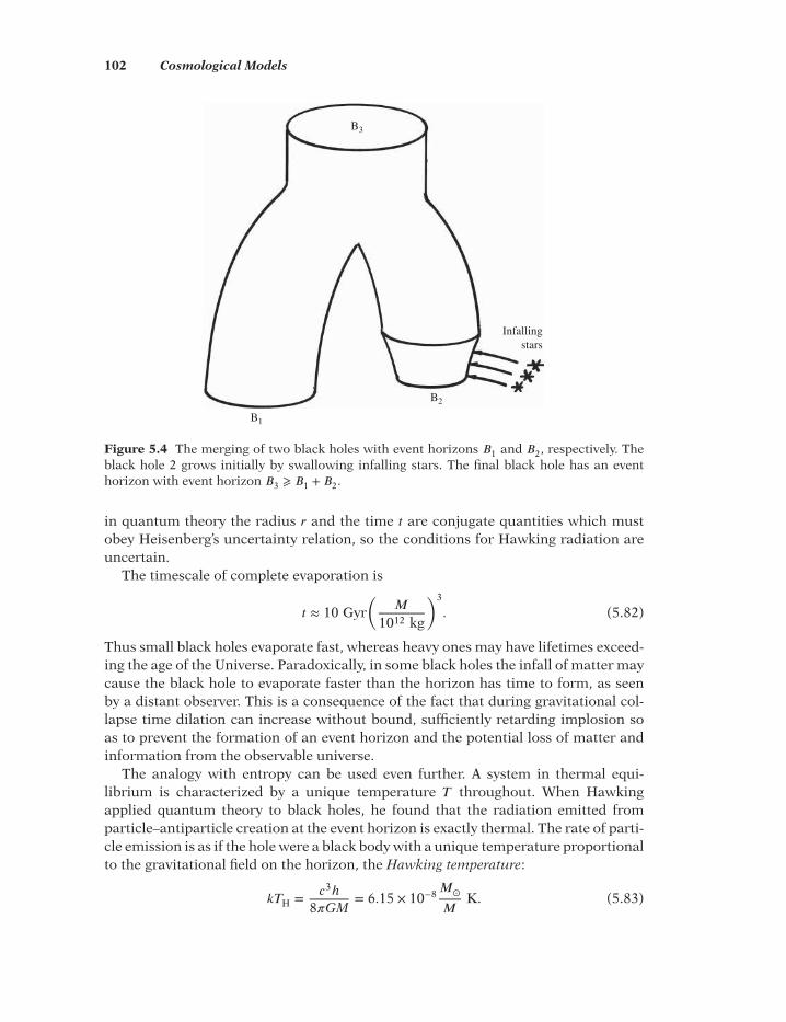
102 Cosmological Models
B1
B2
Infallingstars
B3
Figure 5.4 The merging of two black holes with event horizons 𝐵1 and 𝐵2, respectively. Theblack hole 2 grows initially by swallowing infalling stars. The final black hole has an eventhorizon with event horizon 𝐵3 ⩾ 𝐵1 + 𝐵2.
in quantum theory the radius 𝑟 and the time 𝑡 are conjugate quantities which mustobey Heisenberg’s uncertainty relation, so the conditions for Hawking radiation areuncertain.
The timescale of complete evaporation is
𝑡 ≈ 10 Gyr(
𝑀
1012 kg
)3
. (5.82)
Thus small black holes evaporate fast, whereas heavy ones may have lifetimes exceed-ing the age of the Universe. Paradoxically, in some black holes the infall of matter maycause the black hole to evaporate faster than the horizon has time to form, as seenby a distant observer. This is a consequence of the fact that during gravitational col-lapse time dilation can increase without bound, sufficiently retarding implosion soas to prevent the formation of an event horizon and the potential loss of matter andinformation from the observable universe.
The analogy with entropy can be used even further. A system in thermal equi-librium is characterized by a unique temperature 𝑇 throughout. When Hawkingapplied quantum theory to black holes, he found that the radiation emitted fromparticle–antiparticle creation at the event horizon is exactly thermal. The rate of parti-cle emission is as if the hole were a black body with a unique temperature proportionalto the gravitational field on the horizon, the Hawking temperature:
𝑘𝑇H = 𝑐3ℎ
8𝜋GM= 6.15 × 10⁻⁸𝑀⊙
𝑀K. (5.83)
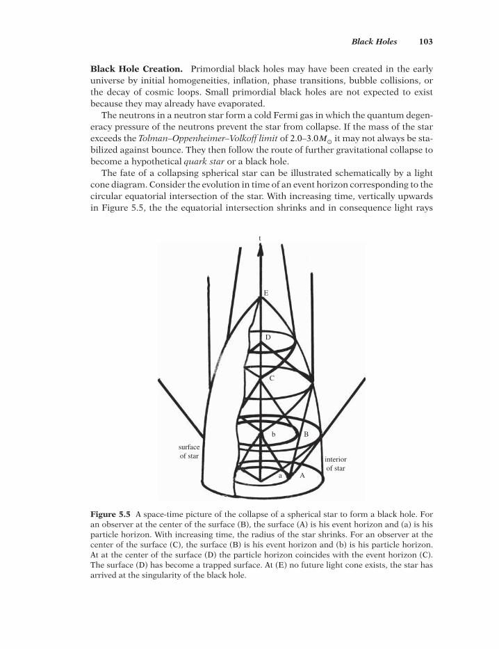
Black Holes 103
Black Hole Creation. Primordial black holes may have been created in the earlyuniverse by initial homogeneities, inflation, phase transitions, bubble collisions, orthe decay of cosmic loops. Small primordial black holes are not expected to existbecause they may already have evaporated.
The neutrons in a neutron star form a cold Fermi gas in which the quantum degen-eracy pressure of the neutrons prevent the star from collapse. If the mass of the starexceeds the Tolman–Oppenheimer–Volkoff limit of 2.0–3.0𝑀
⊙it may not always be sta-
bilized against bounce. They then follow the route of further gravitational collapse tobecome a hypothetical quark star or a black hole.
The fate of a collapsing spherical star can be illustrated schematically by a lightcone diagram. Consider the evolution in time of an event horizon corresponding to thecircular equatorial intersection of the star. With increasing time, vertically upwardsin Figure 5.5, the the equatorial intersection shrinks and in consequence light rays
t
E
D
C
B
Aa
b
surfaceof star interior
of star
Figure 5.5 A space-time picture of the collapse of a spherical star to form a black hole. Foran observer at the center of the surface (B), the surface (A) is his event horizon and (a) is hisparticle horizon. With increasing time, the radius of the star shrinks. For an observer at thecenter of the surface (C), the surface (B) is his event horizon and (b) is his particle horizon.At at the center of the surface (D) the particle horizon coincides with the event horizon (C).The surface (D) has become a trapped surface. At (E) no future light cone exists, the star hasarrived at the singularity of the black hole.

104 Cosmological Models
toward the future steepen. When the star has shrunk to the size of the Schwartzschildradius, the equatorial section has become a trapped surface, the future of all light raysfrom it are directed towards the world line of the center of the star. For an outsideobserver the event horizon then remains eternally of the same size, but an insiderwould find that the trapped surface of the star is doomed to continue its collapsetoward the singularity at zero radius. The singularity has no future light cone andcannot thus ever be observed (Figure 5.5).
Black holes are probably created naturally in the aging of stars. The collapse of anisolated heavy star is, however, not the only route to the formation of a black hole, andprobably not even the most likely one. Binary stars are quite common, and a binarysystem consisting of a neutron star and a red giant is a very likely route to a black hole.The neutron star spirals in (see Figure 5.5), accretes matter from the red giant at a veryhigh rate, about 1𝑀
⊙per year, photons are trapped in the flow, gravity and friction
heat the material in the accretion disc until it emits X-rays. When the temperaturerises above 1 MeV neutrinos can carry off the thermal energy.
For example, Cyg X-1 is a black hole—a main-sequence star binary with a holemass of more than about 10𝑀
⊙, probably the most massive black hole in a binary
observed in the Galaxy. The enormous gravitational pull of the hole tears materialfrom its companion star. This material then orbits the hole in a Saturnus-like accretiondisc before disappearing into the hole. Finally, the main-sequence star explodes andbecomes a neutron star, which will ultimately merge into the hole to form a heavierblack hole.
Neutron stars and stellar black holes have masses of the order of 10𝑀⊙
, supermas-sive black holes have 106−10𝑀
⊙. There could be as many as 108 stellar black holes in
our galaxy. Black holes weighing thousands or million times the Chandrasekhar limitof 1.44𝑀
⊙cannot have been produced in the collapse of a single star. How they have
been produced is currently not well understood. The most likely route is by accretionand coalescence of intermediate mass black holes.
Massive black holes are seen at very high redshift. The discovery of 109𝑀⊙
blackholes at 𝑧 > 7.0 is mysterious since it is unclear how such massive objects could haveformed and grown so quickly at early times.
Observations of Black Holes. Since black holes cannot be seen directly, one has toinfer their existence from indirect evidence. Within our galaxy one can measure theorbits of neighboring individual stars. In this way one has deduced that the centralfew parsecs of our galaxy evidently hosts a dense and luminous star cluster and a verycompact radio source Sgr A∗ [10]. Its intrinsic size is aa most 10 light minutes whichmakes it the most likely candidate of a possible central black hole. There is evidencefor little motion of the Sgr A∗ itself from the size and motions of the central compactradio source.
There are precise determinations of the elliptical orbits and the velocity vectors ofabout 30 stars in the vicinity, all having one common focal point located at the Sgr A∗,see Figure 5.6. All the acceleration vectors intersect at Sgr A∗, and the velocity vectorsdo not decrease with decreasing distance to Sgr A∗, indicating that the stars move in

Black Holes 105
0.175
0.15
0.125
0.1
0.075
0.05
0.025
0
0.05 0.025 –0.025
2001
2005
1992
2010
1995
2002
SgrA*
RA-offset (arcsec)
S2 (S02)
–0.05 –0.0750
Figure 5.6 Orbit of the star S2 moving around Sgr A* [10]. Copyright 2010 by the AmericanPhysical Society. (See plate section for color version.)
a very strong gravitational field of a practically pointlike source of mass 4.4 × 10⁶𝑀⊙
.The best measured orbit of the star 𝑆2 which has completed a full orbit since thebeginning of 1992 is shown in Figure 5.6 [10].
There is a hot accreting zone around the event horizon where Sgr A∗ is accretingfrom the winds of surrounding stars at the outer boundary. Typically the radiatedpower from the accretion zone feeds the luminosity which is very weak both in radioand X-ray emission, but hot, thermal X-ray emission associated with Sgr A∗ has beenclaimed. It appears that there is a dynamically important magnetic field near the blackhole, determining the structure of the accretion flow. If this field is accreted down tothe event horizon it provides enough magnetic flux to explain the observed emission.
At the time of writing, an enigmatic small nonself-gravitating gas cloud is seenfalling almost exactly onto Sgr A∗ at a nominal pericenter distance of only 2200Schwarzschild radii (𝑟c = 136 km). Observations over the next decade should enlightenits fate and allow us to explore general relativity.

106 Cosmological Models
The accretion disks of black holes are typically truncated near the innermostcircular orbit of matter, and hence the main effect is the deformation of a ring thesize of this orbit bending near the black hole, rather than the effect of the event hori-zon itself. There will then be a shadow which is essentially a lensed image of theevent horizon, and its shape is closely related to the closed orbit for photons aroundthe black hole. Since photons that circle the black hole slightly within the photonorbit will end up inside the event horizon while photons just outside will escapeto infinity, there is a rather sharp boundary between bright and dark regions. Theshadow itself is thus indeed primarily a deficit of photons due to absorption by theevent horizon.
A spectral turn-over indicates that the region becomes optically thin and allowsus to see through to the event horizon. The shadow is in principle detectable withpresent-day technology and would allow many fundamental tests of general relativityand its alternatives.
Active galactic nuclei (AGN) furnish other indirect proof for black holes. AGN oftenexhibit quasars which require enormously powerful engines, much more than super-novae could furnish. It is now thought that every AGN is powered by a massive centralblack hole accreting radiation, matter and vacuum energy. The supermassive blackhole Sgr A∗ is, however very inactive, so there is no quasar associated with it.
Spectacular flashes of energies 1000–10 000 larger than those of SNe (1054 erg, orthe release of 1𝑀
⊙in a few 0.1 s) are seen homogeneously distributed in the universe.
These Gamma Ray Bursts have a duration of 10−2 to 102 s. The very first one nearlystarted a third World War when United States intelligence suspected that the SovietUnion was testing a new arm above the Earth.
The GRBs are not ejected from black holes, rather they originate from the grav-itational collapse of a neutron star to a black hole. One possible route for shortGRBs is that they originate from an initial binary system consisting of a compactcarbon–oxygen (CO) core star and a neutron star. The CO core explodes as a super-nova, and part of its ejecta accretes onto the neutron star which reaches its criticalmass and collapses to a black hole. A new neutron star is then generated by the super-nova as a remnant. The energy released in the GRB is energetically dominant to super-novae, so it cannot originate in an SN. Long-duration GRBs are believed to be due toa continued energy injection mechanism which powers the forward shock, giving riseto an unusual and long-lasting afterglow.
If a neutron star and a black hole are gravitationally bound they can give rise to anew process of merging, resulting in a gravitational collapse leading to a new blackhole with the emission of a GRB and possibly gravitational waves.
5.5 Extended Gravity Models
In Chapter 3.3 we derived the Einstein Equation (3.28) from the Einstein–Hilbertaction
𝑆 =∫
d4𝑥√−𝑔
[1
2𝜅𝑅 +
𝑀(𝑔𝜇𝜈, 𝛹 )
], (5.84)

Extended Gravity Models 107
where 𝛹 represents some matter fields. Many proposals have been made to general-ize this action. Suppose that the universe contains a scalar field 𝜙 not present in theEinstein equation. There are then different options how to introduce it, even the met-ric frame may need to be reformulated. Since the Einstein equation describes howmatter affects the geometry and the curvature of space-time, the scalar field in theenergy-momentum tensor will also affect the geometry.
The Robertson–Walker metric in Equation (2.32) determines the geometry ofspace-time by the components 𝑔
𝜇𝜈in Equation (2.33), the affine connections 𝛤𝜇𝜎𝜈 in
Equation (3.13), and the Ricci scalar 𝑅 in (3.18) in what is called the Einstein frame.If the matter field 𝜙 is introduced into the action in such a way that no terms 𝜙𝑅 nor𝐹 (𝜙)𝑅mixing matter and geometry appear, we are in the Einstein frame. The oppositecase is the Jordan frame. The two frames are only mathematically different, becauseone can transform expressions in one frame into one in the other by a conformaltransformation such as ��
𝜇𝜈= 𝜁2(𝑥)𝑔
𝜇𝜈, where 𝜁2(𝑥) is the conformal factor. There is no
physical difference, only a choice of mathematical convenience.Let us now rewrite the Einstein–Hilbert action in the most general form in the
Jordan frame as
𝑆total = ∫d𝑛𝑥
√−𝑔
[1
2𝜅𝑓 (𝑅,𝜙) + phi(𝑔𝜇𝜈, 𝜙, 𝜕𝜙) +
𝑀(𝑔𝜇𝜈, 𝛹 )
]. (5.85)
Here we have replaced the curvature scalar 𝑅 by a general function 𝑓 (𝑅,𝜙), andenlarged the dimensionality of space-time from 4 to 𝑛. The Lagrangian density is thenusually of the form
phi = −𝑀2
2𝜔(𝜙)(𝜕𝜙)2 − 𝑉 (𝜙), (5.86)
where we have denoted (𝜕𝜙)2 ≡ (∇𝛼𝜙)(∇𝛼𝜙). For a canonical scalar field the function 𝜔
equals unity.Two simple versions of extended gravity are those which lack a scalar field 𝜙 but
are nonlinear in 𝑅, and scalar-tensor theories. Some nonlinear functions 𝑓 (𝑅) studiedare of the form (𝑅 + 𝛼𝑅2) and (𝑅 − 𝛼∕𝑅). The dynamical equations are then written inthe Einstein frame.
Scalar-tensor theories are of the form 𝑓 (𝑅,𝜙) = 𝐹 (𝜙)𝑅 in the Jordan frame, of whichthe classical (1961) Brans–Dicke theory with 𝐹 (𝜙) = 𝜙 is the simplest. Some otherexamples of scalar-tensor theories are 𝐹 (𝜙) = exp(−𝜙) and 𝐹 (𝜙) = 𝛼𝜙2.
If the theory has no scalar field 𝜙 one proceeds as for the Einstein–Hilbert action,varying the action 𝑆 with respect to the metric 𝑔
𝜇𝜈and setting the variation equal to
zero. For scalar-tensor theories the equations of motion follow from setting the varia-tion of 𝑆 with respect to 𝜙 equal to zero, and next differentiating the component of theenergy–momentum tensor 𝑇
𝜇𝜈which depends on 𝜙. After that, one again proceeds to
vary the action 𝑆 with respect to the metric 𝑔𝜇𝜈
and setting the variation equal to zero.Note that since the Ricci scalar 𝑅 contains second derivatives of the metric, one
ends up with fourth order terms of the metric which are difficult to analyze. A moretractable form of extended gravity can be obtained by using the Palatini variation. Inthis formulation the affine connection 𝛤𝜇𝜎𝜈 in Equation (3.13) is treated as an indepen-dent variable from the metric 𝑔
𝜇𝜈. Varying the action separately with respect to 𝑔
𝜇𝜈

108 Cosmological Models
and 𝛤𝜇𝜎𝜈 gives a system of second-order differential equations. This will of course giverise to somewhat different physics than the Einstein–Hilbert variation, so in due timewe will probably have data permitting us to decide between them.
Another degree of freedom in the action [Equation (5.85)] is the dimensionality 𝑛of space-time. At this point in my treatise there is no obvious reason to assume that𝑛 is larger than four. However, the gravitational interaction is so much weaker thanall the standard particle interactions, that one could imagine that it propagates in adifferent space-time. We shall come back to models in later chapters which explorethis freedom.
Problems
1. On the solar surface the acceleration caused by the repulsion of a non-vanishingcosmological constant 𝜆 must be much inferior to the Newtonian attraction.Derive a limiting value of 𝜆 from this condition.
2. In Newtonian mechanics, the cosmological constant 𝜆 can be incorporated byadding to gravity an outward radial force on a body of mass 𝑚, a distance 𝑟from the origin, of 𝐹 = +𝑚𝜆𝑟∕6. Assuming that 𝜆 = −10−20 yr−2, and that 𝐹 is theonly force acting, estimate the maximum speed a body will attain if its orbit iscomparable in size with the Solar System (0.5 light day [11]).
3. de Sitter’s static universe has 𝑎 ∝ eHt, zero curvature of its co-moving coordinates(𝑘 = 0), and a proper density of all objects that is constant in time. Show thatthe co moving volume out to red-shift 𝑧 is 𝑉 (𝑧) = 4
3𝜋(cz∕𝐻)3, and hence that the
number-count slope for objects at typical red-shift 𝑧 becomes [(3 + 𝛼) ln 𝑧]−1 for𝑧 ≫ 1, where 𝛼 is the spectral index for the objects [12].
4. Starting from Equation (5.55) with the parameters𝛺0 = 1,𝛺r = 0, show that theage of the Universe can be written
𝑡0 = 23𝐻0
tanh−1√𝛺𝜆√
𝛺𝜆
.
5. A galaxy at 𝑧 = 0.9 contains a quasar showing red-shift 𝑧 = 1.0. Supposing thatthis additional red-shift of the quasar is caused by its proximity to a black hole,how many Schwarzschild radii away from the black hole does the light emittedby the quasar originate?
6. Estimate the gravitational red-shift 𝑧 of light escaping from a galaxy of mass109𝑀
⊙after being emitted from a nearby star at a radial distance of 1 kpc from
the center of the galaxy. (Assume that all matter in the galaxy is contained withinthat distance [11].)
7. Light is emitted horizontally in vacuo near the Earth’s surface, and falls freelyunder the action of gravity. Through what vertical distances has it fallen aftertravelling 1 km? Calculate the radial coordinate (expressed in Schwarzschildradii) at which light travels in a circular path around a body of mass 𝑀 [11].

Extended Gravity Models 109
References[1] Rich, J. 2001 Fundamentals of cosmology. Springer.[2] Solà, J. 2001 Nucl. Phys. B, 95, 29.[3] Cappi, A. 2001 Astrophys. Lett. Commun. 40, 161.[4] Kraniotis, G. V. and Whitehouse, S. B. 2002 Classical Quantum Gravity 19, 5073.[5] Hawking, S. and Penrose, R. 1996 The nature of space and time. Princeton University Press,
Princeton, NJ.[6] Hawking, S. W. Preprint at http://arxiv.org/abs/1401.5761 (2014).[7] Bekenstein, J. 1973 Phys. Rev. D, 7, 2333.[8] Hawking, S. W. 1974 Nature 248, 30.[9] Hawking, S. W. 1975 Commun. Math. Phys. 43, 199.
[10] Genzel, R., Eisenhauer, F. and Gillessen, S., 2010 Rev. Mod. Phys 82, 3121.[11] Berry, M. V. 1989 Principles of cosmology and gravitation. Adam Hilger, Bristol.[12] Peacock, J. A. 1999 Cosmological physics. Cambridge University Press, Cambridge.


6
Thermal Historyof the Universe
This history should start at the Big Bang which we defined in the previous chapter astime zero. General relativity is a classical theory in which the coordinates 𝑡, 𝑥, 𝑦, 𝑧 cantake any real values. However, Equations (5.41) and (5.42) showed that at time zerono meaningful description of the Universe exists.
Actually there are problems already for small but nonzero times, at the energy scalewhere gravitational and quantum effects are of equal importance. Then we can notdo particle physics neglecting gravitation nor can we describe the Universe with theEinstein equation neglecting quantum mechanics.
In Section 6.1 we begin with a definition of the Planck time, leaving the cosmicinflation for a later chapter. In Section 6.2 we continue with the primordial hot plasmawhich deals with particle physics symmetries, photons in thermal equilibrium, energydensities, relativistic versus nonrelativistic particles, spin and statistics, temperatureand time scales.
We follow the cooling plasma until, in Section 6.3, photon and lepton decouplingoccurs. Next comes photon reheating, neutrino decoupling and the recombinationera. We end with a brief discussion on equilibrium theory.
In Section 6.4 we follow the thermal history of the nucleons for the momentousfusion processes in Big Bang nucleosynthesis (BBN) which has left us very importantclues in the form of relic abundances of helium and other light nuclei. The nucleosyn-thesis is really a very narrow bottleneck for all cosmological models, and one whichhas amply confirmed the standard Big Bang model. We find that the baryonic matterpresent since nucleosynthesis is completely insufficient to close the Universe.
In Section 6.5 we try to understand baryosynthesis and the absence of antimatter.
Introduction to Cosmology, Fourth Edition. Matts Roos© 2015 John Wiley & Sons, Ltd. Published 2015 by John Wiley & Sons, Ltd.

112 Thermal History of the Universe
6.1 Planck Time
Recall that in quantum mechanics it is always possible to associate the mass of aparticle 𝑀 with a wave having the Compton wavelength
𝜆 = ℏ
Mc. (6.1)
In other words, for a particle of mass 𝑀 , quantum effects become important at dis-tances of the order of 𝜆. On the other hand, gravitational effects are important at dis-tances of the order of the Schwarzschild radius. Equating the two distances, we findthe scale at which quantum effects and gravitational effects are of equal importance.This defines the Planck mass
𝑀P =√
ℏ𝑐∕𝐺 = 1.221 × 10¹⁹ GeV 𝑐−2
. (6.2)
From this we can derive the Planck energy 𝑀P𝑐2 and the Planck time
𝑡P = 𝜆P∕𝑐 = 5.31 × 10−44 s. (6.3)
Later on we shall make frequent use of quantities at the Planck scale. The reason forassociating these scales with Planck’s name is that he was the first to notice that thecombination of fundamental constants
𝜆P =√
ℏ𝐺∕𝑐3 = 1.62 × 10⁻³⁵ m (6.4)
yielded a natural length scale. The particle symmetry at Planck time is characterizedby all fields except the inflaton field being exactly massless. Only when this symme-try is spontaneously broken in the transition to a lower temperature phase do someparticles become massive.
Unfortunately, there is as yet no theory including quantum mechanics and gravita-tion. Thus we have no description of the Universe before the Planck time, nor of theBig Bang, because of a lack of theoretical tools.
There is strong evidence that this cosmic inflation happened when the energy scaleof the Universe was about three orders of magnitude lower than the Planck scale. Weshall postpone the discussion of inflation to Chapter 7.
6.2 The Primordial Hot Plasma
The primeval Universe may have developed through phases when some symmetry wasexact, followed by other phases when that symmetry was broken. The early cosmol-ogy would then be described by a sequence of phase transitions. Symmetry breakingmay occur through a first-order phase transition, in which the field tunnels through apotential barrier, or through a second-order phase transition, in which the field evolvessmoothly from one state to another, following the curve of the potential.
An important bookkeeping parameter at all times is the temperature, 𝑇 . When wefollow the history of the Universe as a function of 𝑇 , we are following a trajectory in
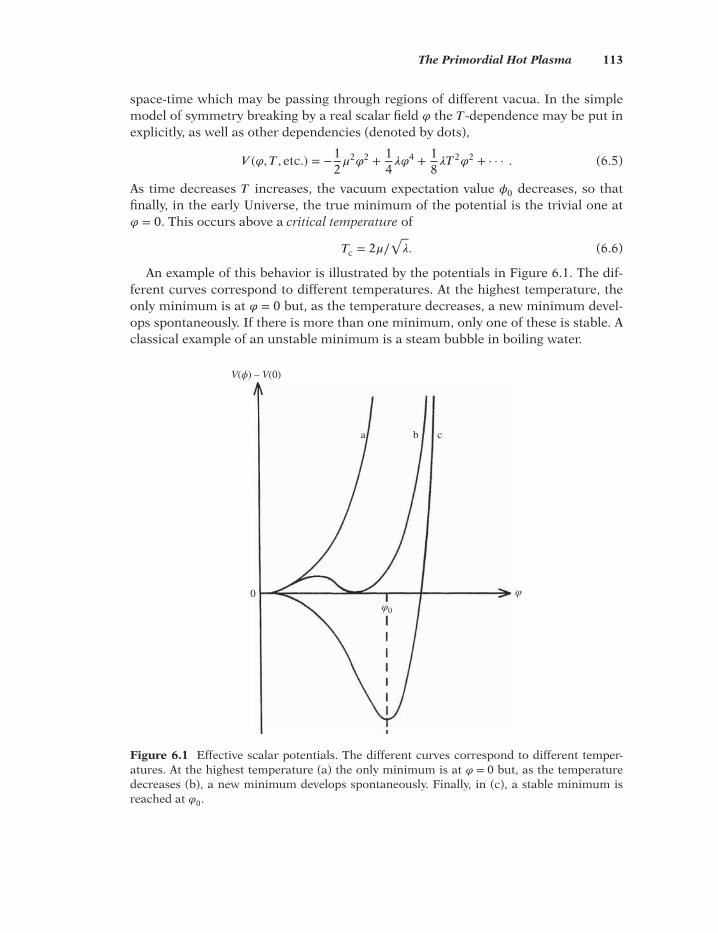
The Primordial Hot Plasma 113
space-time which may be passing through regions of different vacua. In the simplemodel of symmetry breaking by a real scalar field 𝜑 the 𝑇 -dependence may be put inexplicitly, as well as other dependencies (denoted by dots),
𝑉 (𝜑, 𝑇 , etc.) = −12𝜇
2𝜑
2 + 14𝜆𝜑
4 + 18𝜆𝑇
2𝜑
2 + · · · . (6.5)
As time decreases 𝑇 increases, the vacuum expectation value 𝜙0 decreases, so thatfinally, in the early Universe, the true minimum of the potential is the trivial one at𝜑 = 0. This occurs above a critical temperature of
𝑇c = 2𝜇∕√
𝜆. (6.6)
An example of this behavior is illustrated by the potentials in Figure 6.1. The dif-ferent curves correspond to different temperatures. At the highest temperature, theonly minimum is at 𝜑 = 0 but, as the temperature decreases, a new minimum devel-ops spontaneously. If there is more than one minimum, only one of these is stable. Aclassical example of an unstable minimum is a steam bubble in boiling water.
0
a
V(ϕ) – V(0)
b c
φ0
φ
Figure 6.1 Effective scalar potentials. The different curves correspond to different temper-atures. At the highest temperature (a) the only minimum is at 𝜑 = 0 but, as the temperaturedecreases (b), a new minimum develops spontaneously. Finally, in (c), a stable minimum isreached at 𝜑0.

114 Thermal History of the Universe
Particle Physics Symmetries. Above 𝐸 ≈ 1015 GeV the Universe was filled witha plasma of a Grand Unified field of extreme heat and pressure, and occupying anexceedingly small volume. Neither elementary particles nor their more elementaryconstituents were stable under such conditions, only quantum packets of radiativeenergy incessantly exchanging energy existed. Only when the Universe had cooled tobelow 1 TeV the leptons characterized by their electroweak interactions and the quarkscharacterized by their color interactions appeared as constituents in the plasma.
In the energy range 1012 GeV ≲ 𝐸 ≲ 1016 GeV the strengths of the electro-weak forceand the quark color force experienced by photons, leptons and quarks, might havebeen unified in a unique symmetry group 𝐺GUT, with one coupling constant 𝑔. All theleptons and quarks should be components of that same field.
If there is such a symmetry group its mathematical form is not known. Although allGUTs are designed to answer some of the questions and relate some of the parametersin the standard model, they still have the drawback of introducing large numbers ofnew particles, vector bosons and Higgs scalars, all of which have to be discovered.
The global symmetry group in particle physics may have been of the form
𝐺s ≡ SU(3)c ⊗ SU(2)w ⊗𝑈 (1)𝐵−𝐿. (6.7)
This is referred to as the standard model, where the subscripts 𝑐 stands for color, 𝑤 forweak interactions and 𝐵 − 𝐿 for Baryon and Lepton number, respectively. It is consid-ered to be an exact symmetry in the 1 TeV ≲ 𝐸 ≲ 1011−12 TeV energy range. It is lab-oratory physics that has led us to construct the standard model, which is fairly wellunderstood although experimental information above 1 TeV is lacking. Moreover, thestandard model leaves a number of questions open which one would very much liketo have answered within a GUT model.
There are too many free parameters in the standard model. Why are the electriccharges such as they are? How many Higgs scalars are there, more than the one dis-covered in 2012? Why do the leptons and the quarks come in three families. The GUTsymmetry group would require only one family, but if nature provides us with more,why are there precisely three? What is the reason for CP violation? The only hint isthat CP violation seems to require (but not explain) at least three families of quarks.
The big question is what new physics may appear in the enormous range between1 TeV and the GUT energy 1014 GeV. The possibility that nothing new appears is called‘the desert’.
The new physics could be a higher symmetry which would be broken at the lowerend of this energy range. Somewhere there would then be a phase transition betweenthe exactly symmetric phase and the spontaneously broken phase. Even in the case ofa ‘desert’, one expects a phase transition at 1014 or 1015 GeV. One effect which finds itsexplanation in processes at about 1014 GeV is the remarkable absence of antimatterin the Universe.
If the GUT symmetry breaks down to the standard model through intermediatesteps, the phenomenology could be very rich. For instance, there are subconstituentmodels building leptons and quarks out of elementary particles of one level deeperelementarity. These subconstituents would freeze out at some intermediate energy,

The Primordial Hot Plasma 115
condensing into lepton and quark bound states. The forces binding them are in somemodels called technicolor forces.
Below the energy 𝐸 ≈ 1 TeV we encounter the phase transition between exact andspontaneously broken SU(2)w ⊗𝑈 (1)
𝐵−𝐿 symmetry. The end of electroweak unifica-tion is marked by the massification of the vector boson fields, the scalar Higgs fieldsand the fermion fields.
One much discussed extension to the standard model is supersymmetry (SUSY).This brings in a large number of new particles, some of which should be seen in thistemperature range. In this theory there is a conserved multiplicative quantum number,R parity, defined by
𝑅 = (−1)3𝐵+𝐿+2𝑠, (6.8)
where 𝐵, 𝐿 and 𝑠 are baryon number, lepton number and spin, respectively. All knownparticles have 𝑅 = +1, but the theory allows an equal number of supersymmetricpartners, sparticles, having 𝑅 = −1. Conservation of 𝑅 ensures that SUSY sparticlescan only be produced pairwise, as sparticle–antisparticle pairs. The lightest sparticlesmust therefore be stable, just as the lightest particles are.
One motivation for introducing this intermediate scale is the hierarchy problem:why is 𝑚P so enormously much larger than 𝑚W? And why is 𝑉Coulomb so much largerthan 𝑉Newton? SUSY has so many free parameters that it can ‘naturally’ explain theseproblems.
Thermal Equilibrium. Motion of particles under electromagnetic interaction isdescribed by the Maxwell–Lorentz equations. The motion of a particle in a centralfield of force 𝐹 , as for instance an electron of charge 𝑒 moving at a distance 𝑟 aroundan almost static proton, is approximated well by the Coulomb force
𝐹 = 𝑒2
𝑟2. (6.9)
Note that this has the same form as Newton’s law of gravitation, Equation (1.28). Inthe electromagnetic case the strength of the interaction is 𝑒2, whereas the strengthof the gravitational interaction is GM𝑚G. These two coupling constants are expressedin completely different units because they apply to systems of completely differentsizes. For the physics of radiation, the gravitational interaction can be completelyneglected but, for the dynamics of the expansion of the Universe, only the gravitationalinteraction is important because celestial objects are electrically neutral.
The photons and the first particles which formed momentarily in the primordialplasma were incessantly colliding and exchanging energy and momentum at relativis-tic speeds. A few collisions were sufficient to distribute the available energy evenlyamong them. Their reaction rates were much greater than the Hubble expansion rate,so thermal equilibrium should have been maintained in any local comoving volumeelement d𝑉 .
There was no net inflow or outflow of energy, which defines the expansion as adi-abatic adiabatic, as was done in Equation (5.25). The law of conservation of energy

116 Thermal History of the Universe
[Equation (5.24)], also called the first law of thermodynamics, followed by assumingthat matter behaved as an expanding nonviscous fluid at constant pressure 𝑝.
When the collisions resulted in a stable energy spectrum, thermal equilibrium wasestablished and the photons had the blackbody spectrum derived in 1900 by MaxPlanck.
Let the number of photons of energy ℎ𝜈 per unit volume and frequency interval be𝑛𝛾(𝜈). Then the photon number density in the frequency interval (𝜈, 𝜈 + d𝜈) is
𝑛𝛾(𝜈) d𝜈 = 8𝜋
𝑐3
𝜈2 d𝜈eℎ𝜈∕kT − 1
. (6.10)
At the end of the nineteenth century some 40 years was spent trying to find this for-mula using trial and error. With the benefit of hindsight, the derivation is straightfor-ward, based on classical thermodynamics as well as on quantum mechanics, unknownat Planck’s time.
Note that Planck’s formula depends on only one parameter, the temperature 𝑇 . Thusthe energy spectrum of photons in thermal equilibrium is completely characterizedby its temperature 𝑇 . The distribution [Equation (6.10)] peaks at the frequency
𝜈max ≃ 3.32 × 10¹⁰𝑇 (6.11)
in units of Hertz or cycles per second, where 𝑇 is given in degrees Kelvin.The total number of photons per unit volume, or the number density 𝑁
𝛾, is found
by integrating this spectrum over all frequencies:
𝑁𝛾=∫
∞
0𝑛𝛾(𝜈) d𝜈 ≃ 1.202 2
𝜋2
(kT𝑐ℏ
)3
. (6.12)
Here ℏ represents the reduced Planck’s constant ℏ = ℎ∕2𝜋. The temperature 𝑇 maybe converted into units of energy by the dimensional relation 𝐸 = kT. The solution ofthe integral in this equation can be given in terms of Riemann’s zeta-function; 𝜁(3) ≈1.2020.
Since each photon of frequency 𝜈 is a quantum of energy ℎ𝜈 (this is the interpreta-tion Planck was led to, much to his own dismay, because it was in obvious conflict withclassical ideas of energy as a continuously distributed quantity), the total energy den-sity of radiation is given by the Stefan–Boltzmann law after Josef Stefan (1835–1893)and Ludwig Boltzmann (1844–1906),
𝜀r = ∫
∞
0ℎ𝜈𝑛
𝛾(𝜈) d𝜈 = 𝜋
2
15𝑘4𝑇 4
ℏ3𝑐3≡ 𝑎S𝑇
4, (6.13)
where all the constants are lumped into Stefan’s constant
𝑎S = 4723 eV m−3 K−4.
The blackbody spectrum is shown in Figure 8.1.If the expansion is adiabatic and the pressure 𝑝 is constant so that d(pV) = 𝑝 d𝑉 ,
we recover the second law of thermodynamics.The second law of thermodynamics states in particular that entropy cannot
decrease in a closed system. The particles in a plasma possess maximum entropy whenthermal equilibrium has been established. The assumption that the Universe expands

The Primordial Hot Plasma 117
adiabatically is certainly very good during the radiation-dominated era when the fluidwas composed of photons and elementary particles in thermal equilibrium. However,the Universe, black holes and for instance voids are generalized thermodynamic sys-tems for which the equations of thermodynamics must be written in a complete forminvolving a factor due to the expansion of the Universe and a redefinition of entropy.
This is also true during the matter-dominated era before matter clouds start tocontract into galaxies under the influence of gravity. Even on a very large scale wemay consider the galaxies forming a homogeneous ‘fluid’, an idealization as good asthe cosmological principle that forms the basis of all our discussions. In fact, we havealready relied on this assumption in the derivation of the Einstein equation and inthe discussion of equations of state. However, the pressure in the ‘fluid’ of galaxies ofdensity 𝑁 is negligibly small, because it is caused by their random motion, just as thepressure in a gas is due to the random motion of the molecules. Since the averagepeculiar velocities ⟨𝑣⟩ of the galaxies are of the order of 10−3𝑐, the ratio of pressure𝑝 = 𝑚⟨𝑣⟩2𝑁 to matter density 𝜌 gives an equation of state (Problem 5) of the order of
𝑤 ≈𝑚⟨𝑣⟩2𝑁
𝜌𝑐2=
⟨𝑣⟩2
𝑐2≈ 10−6
.
We have already relied on this value in the case of a matter-dominated universe whenderiving Equation (5.30).
Energy Density. Let us compare the energy densities of radiation and matter. Theenergy density of electromagnetic radiation corresponding to one photon in a vol-ume 𝑉 is
𝜌r𝑐2 ≡ 𝜀r =
ℎ𝜈
𝑉= hc
𝑉 𝜆. (6.14)
In an expanding universe with cosmic scale factor 𝑎, all distances scale as 𝑎 and sodoes the wavelength 𝜆. The volume 𝑉 then scales as 𝑎
3; thus 𝜀r scales as 𝑎−4. Here andin the following the subscript ‘r’ stands for radiation and relativistic particles, while‘m’ stands for nonrelativistic (cold) matter.
Statistical mechanics tells us that the pressure in a nonviscous fluid is related tothe energy density by the equation of state [Equation (5.32)]
𝑝 = 13𝜀, (6.15)
where the factor 13
comes from averaging over the three spatial directions. Thus pres-sure also scales as 𝑎−4, so that it will become even more negligible in the future thanit is now. The energy density of matter,
𝜌m𝑐2 = 𝑚𝑐
2
𝑉, (6.16)
also decreases with time, but only with the power 𝑎−3. Thus the ratio of radiationenergy to matter scales as 𝑎
−1:
𝜀r
𝜌m∝ 𝑎
−4
𝑎−3∝ 𝑎
−1. (6.17)

118 Thermal History of the Universe
The present radiation energy density is predominantly in the form of microwavesand infrared light. The change from radiation domination to matter domination isgradual: at 𝑡 = 1000 yr the radiation fraction was about 90%, at 𝑡 = 2 Myr only about10% (see Figure 7.3).
Relativistic versus Nonrelativistic Particles. It is important to distinguishbetween relativistic and nonrelativistic particles because their energy spectra in ther-mal equilibrium are different. A coarse rule is that a particle is nonrelativistic when itskinetic energy is small in comparison with its mass, and relativistic when 𝐸 ≳ 10𝑚𝑐2.The masses of some cosmologically important particles are given in Table A.4. Forcomparison, the equivalent temperatures are also given. This gives a rough idea ofthe temperature of the heat bath when the respective particle is nonrelativistic.
The adiabaticity condition �� = 0 can be applied to both relativistic and nonrela-tivistic particles. Let us first consider the relativistic particles which dominate theradiation era. Recall from Equation (3.9) that the energy of a particle depends on twoterms, mass and kinetic energy,
𝐸 =√
𝑚2𝑐4 + 𝑃 2𝑐2, (6.18)
where 𝑃 is momentum. For massless particles such as the photons, the mass term isof course absent; for relativistic particles it can be neglected.
When 𝑝 is a constant we can write the law of energy conservation
d𝐸 = −𝑝d𝑉 . (6.19)
Replacing 𝐸 by the energy density 𝜀r times the volume 𝑎3 ≡ 𝑉 , the above law becomes
d(𝑎3𝜀r) = −𝑝 d(𝑎3). (6.20)
Substituting 𝜀r for the pressure 𝑝 from the equation of state Equation (6.15) we obtain
𝑎3 d𝜀r + 𝜀r d𝑎3 = −1
3𝜀r d𝑎3
,
or
d𝜀r
𝜀r= −4
3d𝑎3
𝑎3. (6.21)
The solution to this equation is
𝜀r ∝ 𝑎−4
, (6.22)
in agreement with our previous finding. We have in fact already used this result inEquation (5.33).
For nonrelativistic particles the situation is different. Their kinetic energy 𝜀kin issmall, so that the mass term in Equation (6.18) can no longer be neglected. The motionof 𝑛 particles per unit volume is then characterized by a temperature 𝑇m, causinga pressure
𝑝 = nk𝑇m. (6.23)

The Primordial Hot Plasma 119
Note that 𝑇m is not the temperature of matter in thermal equilibrium, but rather abookkeeping device needed for dimensional reasons. The equation of state differsfrom that of radiation and relativistic matter, Equation (6.15), by a factor of 2:
𝑝 = 23𝜀kin.
Including the mass term of the 𝑛 particles, the energy density of nonrelativistic matterbecomes
𝜌m ≡ 𝜀m = nm𝑐2 + 3
2nk𝑇m. (6.24)
Substituting Equations (6.23) and (6.24) into Equation (6.20) we obtain
d(𝑎3nm𝑐2) + 3
2d(𝑎3nk𝑇m) = −nk𝑇m d𝑎3
. (6.25)
Let us assume that the total number of particles always remains the same: in ascattering reaction there are then always two particles coming in, and two going out,whatever their types. This is not strictly true because there also exist other types ofreactions producing more than two particles in the final state. However, let us assumethat the total number of particles in the volume 𝑉 under consideration is 𝑁 = Vn, andthat 𝑁 is constant during the adiabatic expansion,
d𝑁 = d(Vn) = 43𝜋 d(𝑎3
𝑛) = 0. (6.26)
The first term in Equation (6.25) then vanishes and we are left with
32𝑎
3d𝑇m = −𝑇m d(𝑎3),
or
32
d𝑇m
𝑇m= −d(𝑎3)
𝑎3.
The solution to this differential equation is of the form
𝑇m ∝ 𝑎−2
. (6.27)
Thus we see that the temperature of nonrelativistic matter has a different dependenceon the scale of expansion than does the temperature of radiation. This has profoundimplications for one of the most serious problems in thermodynamics in the nine-teenth century.
The number density of relativistic particles other than photons is given by distri-butions very similar to the Planck distribution. Let us replace the photon energy ℎ𝜈 inEquation (6.10) by 𝐸, which is given by the relativistic expression in Equation (6.18).Noting that the kinematic variable is now the three-momentum 𝑝 = |p| (since for rel-ativistic particles we can ignore the mass), we can replace Planck’s distribution by thenumber density of particle species 𝑖 with momentum between 𝑝 and 𝑝 + d𝑝,
𝑛𝑖(𝑝) d𝑝 = 8𝜋
ℎ3
𝑛spin,𝑖
2𝑝2d𝑝
e𝐸𝑖(𝑝)∕𝑘𝑇𝑖 ± 1. (6.28)

120 Thermal History of the Universe
The ± sign is ‘−’ for bosons and ‘+’ for fermions, and the name for these distributionsare the Bose distribution and the Fermi distribution, respectively. The Fermi distribu-tion in the above form is actually a special case: it holds when the number of chargedfermions equals the number of corresponding neutral fermions (the ‘chemical poten-tials’ vanish). In the following we shall need only that case.
The number density 𝑁 of nonrelativistic particles of mass 𝑚 is given by theMaxwell–Boltzmann distribution for an ideal, nondegenerate gas. Starting from Equa-tion (6.28) we note that for nonrelativistic particles the energy kT is smaller than themass, so that the term ±1 in can be neglected in comparison with the exponential.Rewriting the Fermi distribution as a function of temperature rather than of momen-tum we obtain the Maxwell–Boltzmann distribution
𝑁 = 𝑛spin(2𝜋mkT)3∕2
(hc)3e−𝐸𝑖∕𝑘𝑇𝑖 . (6.29)
Note that because of the exponential term the number density falls exponentially astemperature falls. James Clerk Maxwell (1831–1879) was a contemporary of Stefanand Boltzmann.
Thermal Death. Suppose that the Universe starts out at some time with 𝛾 raysat high energy and electrons at rest. This would be a highly ordered nonequilib-rium system. The photons would obviously quickly distribute some of their energyto the electrons via various scattering interactions. Thus the original order woulddecrease, and the randomness or disorder would increase. The second law of ther-modynamics states that any isolated system left by itself can only change towardsgreater disorder. The measure of disorder is entropy; thus the law says that entropycannot decrease.
The counterexample which living organisms seem to furnish, since they build upordered systems, is not valid. This is because no living organism exists in isolation;it consumes nutrients and produces waste. Thus, establishing that a living organismindeed increases entropy would require measurement of a much larger system, cer-tainly not smaller than the Solar System.
It now seems to follow from the second law of thermodynamics that all energywould ultimately distribute itself evenly throughout the Universe, so that no furthertemperature differences would exist. The discoverer of the law of conservation ofenergy, Hermann von Helmholtz (1821–1894), came to the distressing conclusion in1854 that ‘from this point on, the Universe will be falling into a state of eternal rest’.This state was named thermal death, and it preoccupied greatly both philosophers andscientists during the nineteenth century.
Now we see that this pessimistic conclusion was premature. Since 𝐸 scales as 𝑎−1
it follows that also the temperature of radiation 𝑇r scales as 𝑎−1. Thus, from the time
when the temperatures of matter and radiation were equal,
𝑇m = 𝑇r,
we see from Equation (6.27) that the adiabatic expansion of the Universe causes mat-ter to cool faster than radiation. Thus cold matter and hot radiation in an expanding

Electroweak Interactions 121
Universe are not and will never be in thermal equilibrium on a cosmic timescale. Thisresult permits us to solve the adiabatic equations of cold matter and hot radiationseparately, as we in fact have.
6.3 Electroweak Interactions
In quantum electrodynamics (QED) the electromagnetic field is mediated by photonswhich are emitted by a charged particle and absorbed very shortly afterwards byanother. Photons with such a brief existence during an interaction are called virtual,in contrast to real photons.
Virtual particles do not travel freely to or from the interaction region. Energy is notconserved in the production of virtual particles. This is possible because the energyimbalance arising at the creation of the virtual particle is compensated for when itis annihilated, so that the real particles emerging from the interaction region possessthe same amount of energy as those entering the region. We have already met thisargument in the discussion of Hawking radiation from black holes.
However, nature impedes the creation of very huge energy imbalances. For exam-ple, the masses of the vector bosons W± and Z0 mediating the electroweak interactionsare almost 100 GeV. Reactions at much lower energies involving virtual vector bosonsare therefore severely impeded, and much less frequent than electromagnetic interac-tions. For this reason such interactions are called weak interactions.
Real photons interact only with charged particles such as protons p, electrons e−
and their oppositely charged antiparticles, the anti-proton p and the positron e+. Anexample is the elastic Compton scattering of electrons by photons:
𝛾 + e± → 𝛾 + e±. (6.30)
As a result of virtual intermediate states neutral particles may exhibit electromagneticproperties such as magnetic moment. When an electron is captured by a free proton,they form a bound state, a hydrogen atom which is a very stable system. An electronand a positron may also form a bound atom-like state called positronium. This is avery unstable system: the electron and positron are antiparticles, so they rapidly endup annihilating each other according to the reaction
e− + e+ → 𝛾 + 𝛾. (6.31)
Since the total energy is conserved, the annihilation results in two (or three) photonspossessing all the energy and flying away with it at the speed of light.
The reverse reaction is also possible. A photon may convert briefly into a virtuale−e+ pair, and another photon may collide with either one of these charged particles,knocking them out of the virtual state, thus creating a free electron–positron pair:
𝛾 + 𝛾 → e− + e+. (6.32)
This requires the energy of each photon to equal at least the electron (positron) mass,0.51 MeV. If the photon energy is in excess of 0.51 MeV the e−e+ pair will not be createdat rest, but both particles will acquire kinetic energy.

122 Thermal History of the Universe
Protons and anti-protons have electromagnetic interactions similar to positronsand electrons. They can also annihilate into photons, or for instance into an electron–positron pair via the mediation of a virtual photon,
p + p → 𝛾virtual → e− + e+. (6.33)
The reverse reaction is also possible, provided the electron and positron possessenough kinetic energy to create a proton, or 938.3 MeV.
Conservation laws. Note that the total electric charge is conserved throughout thereactions in Equations (6.29)–(6.32). Electric charge can never disappear nor ariseout of neutral vacuum, but it can easily move from a charged particle to a neutral oneas long as that does not violate the conservation of total charge in the reaction. Inthe annihilation of an e−e+ pair into photons, all charges do indeed vanish, but onlybecause the sum of the charges was zero to start with.
There are two further conservation laws governing the behavior of baryons andleptons.
(i) 𝐵 or baryon number is conserved. This forbids the total number of baryonsminus anti-baryons from changing in particle reactions. To help the bookkeep-ing in particle reactions one assigns the value 𝐵 = 1 to baryons and 𝐵 = −1 toanti-baryons in a way analogous to the assignment of electric charges. Photonsand leptons have 𝐵 = 0.
(ii) 𝐿𝑙
or l-lepton number is conserved for each of the lepton flavours 𝑙 = e, 𝜇, 𝜏.This forbids the total number of 𝑙-leptons minus 𝑙-anti-leptons from changingin particle reactions. We assign 𝐿e = 1 to e− and 𝜈e, 𝐿e = −1 to e+ and 𝜈e, andcorrespondingly to the members of the 𝜇 and 𝜏 families. Photons and baryonshave no lepton numbers.
However, there is an amendment to this rule, caused by the complications in thephysics of neutrinos. Although the flavour state 𝑙 is conserved in neutrino reac-tions, it is not conserved in free flight. To observe the flavour state 𝑙 of neutrinos isnot the same as observing the neutrino mass states. There are three neutrino massstates called 𝜈1, 𝜈2, 𝜈3, which are not identical to the flavour states; rather, they arequantum-mechanical superpositions of them. The states are entangled in such a waythat a pure mass state is a mixture of flavour states, and vice versa. Roughly, the 𝜈
𝜇is
the mixture of 14𝜈1, 1
4𝜈2 and 1
2𝜈3.
All leptons participate in the weak interactions mediated by the heavy virtual vectorbosons W± and Z0 and the scalar Higgs boson H0. The Z0 is just like a photon exceptthat it is very massive, about 91 GeV, and the two W± are its 10 GeV lighter chargedpartners. The mass of the H0 is 125 GeV. All these bosons freeze out of thermal equi-librium at 𝐸 ≈ 100 GeV.
There is no difference between weak and electromagnetic interactions: there arecharged-current electroweak interactions mediated by the W±, and neutral-currentinteractions mediated by the Z0, the H0 and the 𝛾. However, the electroweak symmetryis imperfect because of the very different masses.

Electroweak Interactions 123
Weak leptonic reactions are
e± +(−)𝜈e → e± +
(−)𝜈e, (6.34)
(−)𝜈e +
(−)𝜈e →
(−)𝜈e +
(−)𝜈e, (6.35)
where(−)𝜈e stands for 𝜈e or 𝜈e. There is also the annihilation reaction
e− + e+ → 𝜈e + 𝜈e, (6.36)
as well as the reverse pair production reaction.Similar reactions apply to the two other lepton families, replacing e above by 𝜇 or
𝜏, respectively. Note that the 𝜈e can scatter against electrons by the W± exchange andZ0 exchange, respectively. In contrast, 𝜈
𝜇and 𝜈
𝜏can only scatter by the Z0 exchange
diagram, because of the separate conservation of lepton-family numbers.
Spin and Statistics. The leptons and nucleons all have two spin states each. In thefollowing we shall refer to them as fermions, after Enrico Fermi (1901–1954), whereasthe photon, the Higgs boson and the W and Z are bosons, after Satyendranath Bose(1894–1974).
The difference between bosons and fermions is deep and fundamental. The numberof spin states is even for fermions, odd for bosons (except the photon). They behavedifferently in a statistical ensemble. Fermions have antiparticles which most bosonsdo not. The fermion number is conserved, indeed separately for leptons and baryons.The number of bosons is not conserved; for instance, in pp collisions one can produceany number of pions and photons.
Two identical fermions refuse to get close to one another. This is the Pauli exclu-sion force for which Wolfgang Pauli (1900–1958) received the Nobel prize, and whichis responsible for the electron degeneracy pressure in white dwarfs and the neutrondegeneracy pressure in neutron stars. A gas of free electrons will exhibit pressure evenat a temperature of absolute zero. According to quantum mechanics, particles neverhave exactly zero velocity: they always carry out random motions, causing pressure.For electrons in a high-density medium such as a white dwarf with density 106𝜌
⊙, the
degeneracy pressure is much larger than the thermal pressure, and it is enough tobalance the pressure of gravity.
Bosons do not feel such a force, nothing inhibits them getting close to each other.The massive vector bosons W± and Z0 have three spin or polarization states: thetransversal (vertical and horizontal) states which the photons also have, and the lon-gitudinal state along the direction of motion, which the photon is lacking.
The number of distinct states or degrees of freedom, 𝑔, of photons in a statisticalensemble (in a plasma, say) is two. In general, due to the intricacies of quantum statis-tics, the degrees of freedom are the product of the number of spin states, 𝑛spin, thenumber 𝑛anti which is 2 for particles with distinct antiparticles and otherwise 1, anda factor 𝑛Pauli =
78, which only enters for fermions obeying Fermi–Dirac statistics. For
bosons this factor is unity. The degrees of freedom are then
𝑔 = 𝑛spin𝑛anti𝑛Pauli, (6.37)
tabulated in the fifth column of Table A.5.

124 Thermal History of the Universe
For each species of relativistic fermions participating in the thermal equilibriumthere is a specific number density. To find the total number density of particles sharingthe available energy we have to count each particle species 𝑖 weighted by the corre-sponding degrees of freedom 𝑔
𝑖.
Equation (6.13) with a factor 𝑔𝑖explicitly visible is
𝜀𝑖= 1
2𝑔𝑖𝑎S𝑇
4, (6.38)
where 𝑎S is Stefan’s constant. It turns out that this expression gives the correct energydensity for every particle species if we insert its respective value of 𝑔
𝑖from Table A.5.
Equation (6.12) can be correspondingly generalized to relativistic fermions. Theirnumber density is
𝑁f =34𝑁
𝛾. (6.39)
In general, the primordial plasma was a mixture of particles, of which some are rel-ativistic and some nonrelativistic at a given temperature. Since the number densityof a nonrelativistic particle [given by the Maxwell–Boltzmann distribution, Equation(6.28)] is exponentially smaller than that of a relativistic particle, it is a good approx-imation to ignore nonrelativistic particles. Different species 𝑖 with mass 𝑚
𝑖have a
number density which depends on 𝑚𝑖∕𝑇 , and they may have a thermal distribution
with a temperature 𝑇𝑖
different from that of the photons. Let us define the effectivedegrees of freedom of the mixture as
𝑔∗ =∑
bosons 𝑖
𝑔𝑖+
∑fermions 𝑗
𝑔𝑗
(𝑇𝑗
𝑇
)4
. (6.40)
As explained in the context of Equation (6.37) the sum over fermions includes a fac-tor 7
8, accounting for the difference between Fermi and Bose statistics. The factor
(𝑇𝑗∕𝑇 )4 applies only to neutrinos, which obtain a different temperature from the pho-
tons when they freeze out from the plasma (as we shall see later). Thus the energydensity of the radiation in the plasma is
𝜀r =12𝑔∗𝑎S𝑇
4. (6.41)
The sum of degrees of freedom of a system of particles is of course the numberof particles multiplied by the degrees of freedom per particle. Independently of thelaw of conservation of energy, the conservation of entropy implies that the energy isdistributed equally between all degrees of freedom present in such a way that a changein degrees of freedom is accompanied by a change in random motion, or equivalentlyin temperature.
Thus entropy is related to order: the more degrees of freedom there are present, themore randomness or disorder the system possesses. When an assembly of particles(such as the molecules in a gas) does not possess energy other than kinetic energy(heat), its entropy is maximal when thermal equilibrium is reached. For a system ofgravitating bodies, entropy increases by clumping, maximal entropy correspondingto a black hole.

Electroweak Interactions 125
Temperature and Time Scales. Let us now derive a relation between the temper-ature scale and the timescale. We have already found the relation (5.40) between thesize scale 𝑅 and the timescale 𝑡 during the radiation era,
𝑎(𝑡) ∝√
𝑡, (6.42)
where we choose to omit the proportionality factor. The Hubble parameter can thenbe written
𝐻 = ��
𝑎= 1
2𝑡. (6.43)
Note that the proportionality factor omitted in Equation (6.42) has dropped out.In Equation (5.35) we noted that the curvature term 𝑘𝑐
2∕𝑅2 in Friedmann’s equa-tions is negligibly small at early times during the radiation era. We then obtained thedynamical relation
��
𝑎=(
8𝜋𝐺3
𝜌
)1∕2
. (6.44)
Inserting Equation (6.43) on the left and replacing the energy density 𝜌 on the rightby 𝜀r∕𝑐2, we find the relation sought between photon temperature and time:
1𝑡=
√16𝜋𝐺𝑎S
3𝑐2𝑔∗ 𝑇
2 = 3.07 × 10⁻²¹√𝑔∗
𝑇2
[K2][s−1]. (6.45)
The sum of degrees of freedom of a system of particles is of course the numberof particles multiplied by the degrees of freedom per particle. Independently of thelaw of conservation of energy, the conservation of entropy implies that the energy isdistributed equally between all degrees of freedom present in such a way that a changein degrees of freedom is accompanied by a change in random motion, or equivalentlyin temperature.
Thus entropy is related to order: the more degrees of freedom there are present, themore randomness or disorder the system possesses. When an assembly of particles(such as the molecules in a gas) does not possess energy other than kinetic energy(heat), its entropy is maximal when thermal equilibrium is reached. For a system ofgravitating bodies, entropy increases by clumping, maximal entropy correspondingto a black hole.
Cooling Plasma. At a temperature of 1011 K, which corresponds to a mean energyof about 300 MeV, the particles contributing to the effective degrees of freedom 𝑔∗are the photon, three charged leptons, three neutrinos (not counting their three inertright-handed components), the six quarks with three colors each, the gluon of eightcolors and two spin states, the scalar Higgs boson H0, and the vector gauge bosonsW±, Z0. Thus the effective degrees of freedom is given by
𝑔∗ = 2 + 3 × 72+ 3 × 7
4+ 6 × 3 × 7
2+ 8 × 2 + 1 + 3 × 3 = 106.75. (6.46)
Above the QCD–hadron phase transition at 200 MeV the hadrons are representedby their free quark subconstituents which contribute more degrees of freedom than

126 Thermal History of the Universe
hadrons, forming a dense medium of quark matter. Below the transition the quarksbecome bound in hadronic matter, the separation between quarks in the nucleonsincreases, and the interaction between any two quarks in a nucleon cease to interactwith quarks in neighboring nucleons. The degrees of freedom 𝑔∗(𝑇 ) are then reducedsteeply to 69/4 as is shown in Figure 6.2 [1].
Quark matter may still exist today in the core of cold but dense stellar objects suchas neutron stars.
The color symmetry SU(3)c is valid and unbroken at this temperature, but it is in noway apparent, because the hadrons are color-neutral singlets. The color force medi-ated by gluons is also not apparent: a vestige of QCD from earlier epochs remains inthe form of strong interactions between hadrons. It appears that this force is mediatedby mesons, themselves quark bound states.
There is no trace of the weak symmetry SU(2)w, so the weak and electromagneticinteractions look quite different. Their strengths are very different, and the massesof the leptons are very different. Only the electromagnetic gauge symmetry 𝑈 (1) isexactly valid, as is testified to by the conservation of electric charge.
All electrons and photons have an energy below the threshold for proton–anti-proton production [see Equation (6.33)]. Then the number of protons, neutronsand anti-nucleons will no longer increase as a result of thermal collisions, they canonly decrease.
We can follow the evolution of the function 𝑔∗(𝑇 ) in Figure 6.2 [1]. Actually all theparticles in thermal equilibrium contribute, not only those accounted for in Equa-tion (6.61), but also heavier particles which are thermalized by energetic photons andpions in the tail of their respective Boltzmann distributions.
100
50
20g*
g*
g*S
10
5
5 4 3 2
log T
0 –1 –21
Figure 6.2 The evolution of the effective degrees of freedom contributing to the energy density,𝑔∗(𝑇 ) and to the entropy density, 𝑔∗S(𝑇 ), as functions of log 𝑇 , where the temperature is in unitsof MeV [1].

Electroweak Interactions 127
At this time the number density of nucleons decreases quickly because they havebecome nonrelativistic. Consequently, they have a larger probability of annihilatinginto lepton pairs, pion pairs or photons. Their number density is then no longer givenby the Fermi distribution [Equation (6.28)], but by the Maxwell–Boltzmann distribu-tion, Equation (6.29). As can be seen from the latter, when 𝑇 drops below the mass,the number density decreases rapidly because of the exponential factor. If there hadbeen exactly the same number of nucleons and anti-nucleons, we would not expectmany nucleons to remain to form matter. But, since we live in a matter-dominatedUniverse, there must have been some excess of nucleons early on. Note that neutronsand protons exist in equal numbers at the time under consideration.
Although the nucleons are very few, they still participate in electromagnetic reac-tions such as the elastic scattering of electrons,
e± + p → e± + p, (6.47)
and in weak charged current reactions in which charged leptons and nucleons changeinto their neutral partners, and vice versa, as in
e− + p → 𝜈e + n, (6.48)
𝜈e + p → e+ + n. (6.49)
Other such reactions are obtained by reversing the arrows, and by replacing e± by 𝜇±
or 𝜈e by 𝜈𝜇
or 𝜈𝜏. The nucleons still participate in thermal equilibrium, but they are
too few to play any role in the thermal history any more.Below the pion mass (actually at about 70 MeV) the temperature in the Universe
cools below the threshold for pion production:
(e− + e+) or (𝜇− + 𝜇+) → 𝛾virtual → 𝜋
+ + 𝜋−. (6.50)
The reversed reactions, pion annihilation, still operate, reducing the number of pions.However, they disappear even faster by decay. This is always the fate when such lighterstates are available, energy and momentum, as well as quantum numbers such aselectric charge, baryon number and lepton numbers, being conserved. The pion, themuon and the tau lepton are examples of this. The pion decays mainly by the reactions
𝜋− → 𝜇
− + 𝜈𝜇, 𝜋
+ → 𝜇+ + 𝜈
𝜇. (6.51)
Thus 𝑔∗ decreases by 3 to 574
. The difference in mass between the initial pion and thefinal state particles is
𝑚𝜋− 𝑚
𝜇− 𝑚
𝜈= (139.6 − 105.7 − 0.0) MeV = 33.9 MeV, (6.52)
so 33.9 MeV is available as kinetic energy to the muon and the neutrino. This makesit very easy for the 𝜋
± to decay, and in consequence its mean life is short, only 0.026 μs(the 𝜋0 decays even faster). This is much less than the age of the Universe at 140 MeV,which is 23 μs from Equation (6.45). Note that the appearance of a charged leptonin the final state forces the simultaneous appearance of its anti-neutrino in order toconserve lepton number.

128 Thermal History of the Universe
Also, the muons decay fast compared with the age of the Universe, with a lifetimeof 2.2 μs, by the processes
𝜇− → e− + 𝜈e + 𝜈
𝜇, 𝜇
+ → e+ + 𝜈e + 𝜈𝜇. (6.53)
Almost the entire mass of the muon, or 105.7 MeV, is available as kinetic energy tothe final state particles. This is the reason for its short mean life. Here again the con-servation of lepton numbers, separately for the e-family and the 𝜇-family, is observed.
Below the muon mass (actually at about 50 MeV), the temperature in the Universecools below the threshold for muon-pair production:
e− + e+ → 𝛾virtual → 𝜇+ + 𝜇
−. (6.54)
The time elapsed is less than a millisecond. When the muons have disappeared, wecan reduce 𝑔∗ by 7
2to 43
4.
From the reactions in Equations (6.51) and (6.53) we see that the end productsof pion and muon decay are stable electrons and neutrinos. The lightest neutrino 𝜈1
is certainly stable, and the same is probably also true for 𝜈2 and 𝜈3. When this hastaken place we are left with those neutrinos and electrons that only participate inweak reactions, with photons and with a very small number of nucleons. The numberdensity of each lepton species is about the same as that of photons.
6.4 Photon and Lepton Decoupling
The considerations about which particles participate in thermal equilibrium at a giventime depend on two timescales: the reaction rate of the particle, taking into accountthe reactions which are possible at that energy, and the expansion rate of the Universe.If the reaction rate is slow compared with the expansion rate, the distance betweenparticles grows so fast that they cannot find each other.
Reaction Rates. The expansion rate is given by 𝐻 = ��∕𝑎, and its temperature depen-dence by Equations (6.44) and (6.45). The average reaction rate can be written
𝛤 = ⟨Nv𝜎(𝐸)⟩, (6.55)
where 𝜎(𝐸) is the reaction cross-section. The product of 𝜎(𝐸) and the velocity 𝑣 ofthe particle varies over the thermal distribution, so one has to average over it, as isindicated by the angle brackets. Multiplying this product by the number density 𝑁 ofparticles per m3, one obtains the mean rate 𝛤 of reacting particles per second, or themean collision time between collisions, 𝛤 −1.
The weak interaction cross-section turns out to be proportional to 𝑇2,
𝜎 ≃𝐺
2F(kT)2
𝜋(ℏ𝑐)4, (6.56)
where 𝐺F is the Fermi coupling measuring the strength of the weak interaction. Thenumber density of the neutrinos is proportional to 𝑇
3 according to Equations (6.12)and (6.39). The reaction rate of neutrinos of all flavours then falls with decreasingtemperature as 𝑇
5.

Photon and Lepton Decoupling 129
The condition for a given species of particle to remain in thermal equilibrium isthen that the reaction rate 𝛤 is larger than the expansion rate 𝐻 , or equivalently that𝛤
−1 does not exceed the Hubble distance 𝐻−1,
𝛤
𝐻≳ 1. (6.57)
Inserting the 𝑇5 dependence of the weak interaction rate 𝛤wi and the 𝑇
2 dependenceof the expansion rate 𝐻 from Equation (6.45), we obtain
𝛤wi
𝐻∝ 𝑇
3. (6.58)
Thus there may be a temperature small enough that the condition in Equation (5.62)is no longer fulfilled.
Photon Reheating. Photons with energies below the electron mass can no longerproduce e+–e− pairs, but the energy exchange between photons and electrons stillcontinues by Compton scattering, reaction in Equation (6.30), or Thomson scattering,as it is called at very low energies. Electromagnetic cross-sections (subscript ‘em’) areproportional to 𝑇 −2, and the reaction rate is then proportional to 𝑇 , so
𝛤em
𝐻∝ 1
𝑇.
Contrary to the weak interaction case in Equation (6.58), the condition in Equa-tion (6.57) is then satisfied for all temperatures, so electromagnetic interactions neverfreeze out. Electrons only decouple when they form neutral atoms during the Recom-bination Era and cease to scatter photons. The term recombination is slightly mis-leading, because the electrons have never been combined into atoms before. The termcomes from laboratory physics, where free electrons and ionized atoms are created byheating matter (and upon subsequent cooling the electrons and ions recombine intoatoms) or from so-called HII regions, where interstellar plasma is ionized by ultra-violet radiation and characteristic recombination radiation is emitted when electronsand ions re-form.
The exothermic electron–positron annihilation, reaction in Equation (6.31), is nowof mounting importance, creating new photons with energy 0.51 MeV. This is higherthan the ambient photon temperature at that time, so the photon population getsreheated. To see just how important this reheating is, let us turn to the law of conser-vation of entropy.
Making use of the equation of state for relativistic particles (6.15), the entropy canbe written
𝑆 = 4𝑉3kT
𝜀plasma.
Substituting the expression for 𝜀plasma from Equation (6.41) one obtains
𝑆 =2𝑔∗3
𝑉 𝑎S𝑇4
kT, (6.59)
which is valid where we can ignore nonrelativistic particles. Now 𝑎S𝑇4 is the energy
density, so 𝑉 𝑎S𝑇4 is energy, just like kT, and thus 𝑉 𝑎S𝑇
4∕kT is a constant. 𝑔∗ is also

130 Thermal History of the Universe
a constant, except at the thresholds where particle species decouple. The physicalmeaning of entropy of a system is really its degrees of freedom multiplied by someconstant, as one sees here. In Equation (6.12) we saw that the entropy density canalso be written
𝑠 ≡𝑆
𝑉= 3
2𝜁(3)𝑔
𝛾𝑁
𝛾, (6.60)
where 𝑁𝛾
is the number density of photons. Between two decoupling thresholds wethen have
d𝑆d𝑡
= dd𝑡
(2𝑔∗3
𝑉 𝑎S𝑇3
𝑘
)= 0. (6.61)
The second law of thermodynamics requires that entropy should be conserved inreversible processes, also at thresholds where 𝑔∗ changes. This is only possible if 𝑇
also changes in such a way that 𝑔∗𝑇3 remains a constant. When a relativistic particle
becomes nonrelativistic and disappears, its entropy is shared between the particlesremaining in thermal contact, causing some slight slowdown in the cooling rate. Pho-tons never become nonrelativistic; neither do the practically massless neutrinos, andtherefore they continue to share the entropy of the Universe, each species conservingits entropy separately.
Let us now apply this argument to the situation when the positrons and most ofthe electrons disappear by annihilation below 0.2 MeV. We denote temperatures andentropies just above this energy by a subscript ‘+’, and below it by ‘−’. Above thisenergy, the particles in thermal equilibrium are 𝛾, e−, e+. Then the entropy
𝑆 = 23
(2 + 7
2
)𝑉 𝑎S𝑇
3+
𝑘. (6.62)
Below that energy, only photons contribute the factor 𝑔∗ = 2. Consequently, the ratioof entropies 𝑆+ and 𝑆− is
𝑆+
𝑆−= 11
4
(𝑇+
𝑇−
)3
. (6.63)
But entropy must be conserved so this ratio must be unity. It then follows that
𝑇− =(
114
)1∕3
𝑇+ = 1.40𝑇+. (6.64)
Thus the temperature 𝑇𝛾
of the photons increases by a factor of 1.40 as the Universecools below the threshold for electron–positron pair production. Actually, the tem-perature increase is so small and so gradual that it only slows down the cooling ratetemporarily.
Neutrino Decoupling. When the neutrinos no longer obey the condition in Equa-tion (6.57) they decouple or freeze out from all interactions, and begin a free expan-sion. The decoupling of 𝜈
𝜇and 𝜈
𝜏occurs at about 3.8 MeV, whereas the 𝜈e decouple at
2.3 MeV. This can be depicted as a set of connecting baths containing different parti-cles, and having valves which close at given temperatures (see Figure 6.3).

Photon and Lepton Decoupling 131
eγ
A
vμ vτ
ve
B
Figure 6.3 A system of communicating vessels illustrating particles in thermal equilibrium(from K. Kainulainen, unpublished research). At about 3.8 MeV, valve A closes so that 𝜈
𝜇and 𝜈
𝜏
decouple. At 2.3 MeV, valve B closes so that 𝜈e also decouples, leaving only e− and 𝛾 in thermalcontact.
At decoupling, the neutrinos are still relativistic, since they are so light (Table A.3).Thus their energy distribution is given by the Fermi distribution, Equation (6.28), andtheir temperature equals that of the photons, 𝑇
𝜈= 𝑇
𝛾, decreasing with the increasing
scale of the Universe as 𝑎−1. But the neutrinos do not participate in the reheating
process, and they do not share the entropy of the photons, so from now on they remaincolder than the photons:
𝑇𝜈= 𝑇
𝛾∕1.40. (6.65)
The number density 𝑁𝜈
of neutrinos can be calculated as in Equation (6.12) usingEquation (6.10), except that the −1 term in Equation (6.10) has to be replaced by +1,which is required for fermions [see Equation (6.28)]. In the number density distribu-tions [Equations (6.10) and (6.28)], we have ignored possible chemical potentials forall fermions, which one can do for a thermal radiation background; for neutrinos itis an unproven assumption that nonetheless appears in reasonable agreement withtheir oscillation parameters.
The result is that 𝑁𝜈
is a factor of 34
times 𝑁𝛾
at the same temperature. Takingthe difference between temperatures 𝑇
𝜈and 𝑇
𝛾into account and noting from Equa-
tion (6.12) that 𝑁𝛾
is proportional to 𝑇 3, one finds
𝑁𝜈= 3
44
11𝑁
𝛾. (6.66)
After decoupling, the neutrino contribution to 𝑔∗ decreases because the ratio 𝑇𝑖∕𝑇
in Equation (6.40) is now less than one. Thus the present value is
𝑔∗(𝑇0) = 2 + 374
(4
11
)4∕3
= 3.36. (6.67)
The entropy density also depends on 𝑔∗, but now the temperature dependence forthe neutrino contribution in Equation (6.40) is (𝑇
𝑖∕𝑇 )3 rather than a power of four. The
effective degrees of freedom are in that case given by Equation (6.67) if the power 43
is replaced by 1. This curve is denoted 𝑔∗S in Figure 6.2.

132 Thermal History of the Universe
The density parameter is
𝛺𝜈= 3
11
𝑁𝛾
𝜌cℎ2
∑𝑖
𝑚𝑖. (6.68)
Recombination Era. As long as there are free electrons, the primordial photonsare thermalized by Thomson scattering against them, and this prohibits the electronsfrom decoupling, in contrast to neutrinos. Each scattering polarizes the photons, buton average this is washed out. The electromagnetic reaction rate is much higher thanthe weak reaction rate of the neutrinos; in fact, it is higher than the expansion rate ofthe Universe, so the condition in Equation (6.57) is fulfilled.
Eventually the Universe expands and cools to such an extent, to about 1000 K, thatelectrons are captured into atomic orbits, primarily by protons but also by the traceamounts of ionized helium and other light nuclei. This process is referred to as recom-bination. Unlike the unstable particles 𝑛, 𝜋, 𝜇 that decay spontaneously liberatingkinetic energy in exothermic reactions, the hydrogen atom H is a bound state of aproton and an electron. Its mass is less than the p and e− masses together,
𝑚H − 𝑚p − 𝑚e = −13.59 eV, (6.69)
so it cannot disintegrate spontaneously into a free proton and a free electron. Themass difference in Equation (6.69) is the binding energy of the hydrogen atom.
The physics of recombination is somewhat subtle. Initially one might think thatrecombination occurs when the photon temperature drops below 13.59 eV, makingformation of neutral hydrogen energetically favorable. Two characteristics of thephysics push the recombination temperature lower. The first, and the easiest to elabo-rate, is that there are vastly more photons than electrons and so in thermal equilibriumeven a small proportion of high-energy photons are sufficient to maintain effectivelycomplete ionization. Photons in thermal equilibrium have the blackbody spectrumgiven by Equation (6.10). Even for photon temperatures somewhat below 13.59 eVthere will be enough highly energetic photons in the Wein tail (as the high-energy sec-tion is termed) to ionize any neutral hydrogen. The large amount of entropy in theUniverse also favors free protons and electrons.
With respect to the thermal history of the Universe, the fact that photons do notscatter against neutral atoms is critical. As recombination proceeds and the number ofelectrons falls, matter and radiation decouple. This has two results. First, with matterand radiation no longer in thermal equilibrium the thermal history of the two proceedindependently. Perturbations in matter are no longer damped by interaction withradiation and any such perturbations can grow into structures through gravitationalinstability. Decoupling thus initiates the period of structure formation that has led toour present Universe being populated with stars, galaxies, galaxy clusters and so on.
The second result is that, with photons no longer scattering against a sea of elec-trons, the photons can stream freely through the Universe; upon recombination, theUniverse becomes transparent to light. Prior to recombination, the Universe wasopaque to electromagnetic radiation (although not to neutrinos) and it would havebeen impossible to do astronomy if this situation had persisted until today. The freely

Photon and Lepton Decoupling 133
streaming photons from this era form the CMB radiation and their point of lastcontact with matter forms an isotropic last scattering surface (LSS). The era of recom-bination provides a crucial observational limit beyond which we cannot hope to seeusing electromagnetic radiation. The LSS is not a sharp boundary and does not existat a unique redshift. Once the conditions for recombination have been met in one por-tion they should be also met in any other—thus isotropicity. The reason for seeing thisas a theoretical spherical shell is that only one specific shell at one specific distancecan be seen by any specific observer at any specific time. The photons from the LSSpreserve the polarization they incurred in the last Thomson scattering. This remain-ing primordial polarization is an interesting detectable signal, albeit much weakerthan the intensity of the thermalized radiation.
The LSS of the Universe has an exact analogue in the surface of the Sun. Photonsinside the Sun are continuously scattered, so it takes millions of years for some pho-tons to reach the surface. But once they do not scatter any more they continue instraight lines (really on geodesics) towards us. Therefore, we can see the surface ofthe Sun, which is the LSS of the solar photons, but we cannot see the solar interior.We can also observe that sunlight is linearly polarized. In contrast, neutrinos hardlyscatter at all in the Sun, thus neutrino radiation brings us a clear (albeit faint withpresent neutrino detectors) picture of the interior of the Sun.
Equilibrium Theory. An analysis based on thermal equilibrium, the Saha equa-tion, implies that the temperature must fall to about 0.3 eV before the proportion ofhigh-energy photons falls sufficiently to allow recombination to occur. The Saha anal-ysis also implies that the time (or energy or redshift) for decoupling and last scatteringdepend on cosmological parameters such as the total cosmic density parameter 𝛺0,the baryon density 𝛺b, and the Hubble parameter. However, a second feature of thephysics of recombination implies that the equilibrium analysis itself is not sufficient.
The Saha analysis describes the initial phase of departure from complete ionizationbut, as recombination proceeds, the assumption of equilibrium ceases to be appro-priate [see, e.g., Equation (6.9)]. Paradoxically, the problem is that electromagneticinteractions are too fast (in contrast with the weak interaction that freezes out fromequilibrium because of a small cross-section). A single recombination directly to theground state would produce a photon with energy greater than the 13.59 eV bindingenergy and this photon would travel until it encountered a neutral atom and ionizedit. This implies that recombination in an infinite static universe would have to proceedby smaller intermediate steps (thus not directly to the ground state).
In fact the situation is even worse, because reaching the ground state by single pho-ton emission requires transition from the 2P to 1S levels and thus production of pho-tons with energy at least 10.2 eV (Lyman 𝛼 with 𝜆 = 1216 Å). As these photons becomeabundant they will re-ionize any neutral hydrogen through multiple absorption and soit would seem that recombination will be, at a minimum, severely impeded. (Recom-bination in a finite HII region is different because the Ly𝛼 photons can escape.)
There is an alternative path, however. Two-photon emission generated by the 2S →1S transition produces lower-energy photons. The process is slow (with a lifetimeof approximately 0.1 s), so recombination proceeds at a rate quite different from the

134 Thermal History of the Universe
Saha prediction. Consequently, all the times predicted by this nonequilibrium analysisdiffers notably from the Saha prediction, but, interestingly, in such a way that thetimes of decoupling and last scattering have practically no dependence on cosmolog-ical parameters.
Summary. Recombination, decoupling and last scattering do not occur at the exactlysame time. It should also be noted that these terms are often used interchangeably inthe literature, so what we refer to as the LSS is sometimes called the time of recom-bination or decoupling. Recombination can be defined as the time when 90% of theelectrons have combined into neutral atoms. This occurred at redshift
𝑧recombination ≈ 1100. (6.70)
Last scattering is defined as the time when photons start to stream freely. Thisoccurred at redshift
𝑧LSS = 1089, (6.71)
when the Universe was 379 000(𝛺0ℎ2)−1∕2 years old and at a temperature of 0.26 eV,
thus right after the recombination time.Decoupling is defined as the time when the reaction rate (scattering) fell below
the expansion rate of the Universe and matter fell out of thermal equilibrium withphotons. This occurred at redshift
𝑧decoupling ≈ 890. (6.72)
All three events depend on the number of free electrons (the ionization fraction) butin slightly different ways. As a result these events do not occur at exactly the sametime, but close enough to explain the confusion in naming.
The build up of structures started right after decoupling. Reionization of theUniverse occurred at 𝑧reionization = 20 ± 5 and the matter structures were in place at𝑧structures = 5.
6.5 Big Bang Nucleosynthesis
Let us now turn to the fate of the remaining nucleons. Note that the charged currentreactions in Equations (6.47) and (6.48) changing a proton to a neutron are endother-mic: they require some input energy to provide for the mass difference. In the reactionin Equation (6.48) this difference is 0.8 MeV and in reaction in Equation (6.49) it is1.8 MeV (use the masses in Table A.4!). The reversed reactions are exothermic. Theyliberate energy and they can then always proceed without any threshold limitation.
The neutrons and protons are then nonrelativistic, so their number densities areeach given by Maxwell–Boltzmann distributions [Equation (6.29)]. Their ratio in equi-librium is given by
𝑁n
𝑁p=
(𝑚n
𝑚p
)3∕2
exp(−𝑚n − 𝑚p
kT
). (6.73)

Big Bang Nucleosynthesis 135
At energies of the order of 𝑚n − 𝑚p = 1.293 MeV or less, this ratio is dominated by the
exponential. Thus, at kT = 0.8 MeV, the ratio has dropped from 1 to 15. As the Universe
cools and the energy approaches 0.8 MeV, the endothermic neutron-producing reac-tions stop, one by one. Then no more neutrons are produced but some of those thatalready exist get converted into protons in the exothermic reactions.
Nuclear Fusion. Already, at a few MeV, nuclear fusion reactions start to build uplight elements. These reactions are exothermic: when a neutron and a proton fuse intoa bound state some of the nucleonic matter is converted into pure energy accordingto Einstein’s formula [Equation (3.8)]. This binding energy of the deuteron d,
𝑚p + 𝑚n − 𝑚d = 2.22 MeV, (6.74)
is liberated in the form of radiation:
n + p → d + 𝛾. (6.75)
The deuteron is also written 2H+ in general nuclear physics notation, where the super-script 𝐴 = 2 indicates the number of nucleons and the electric charge is given by thesuperscript ‘+’. The bound state formed by a deuteron and an electron is the deuteriumatom 2H, which of course is electrically neutral. Although the deuterons are formedin very small quantities, they are of crucial importance to the final composition ofmatter.
As long as photons of 2.22 MeV or more are available, the reaction in Equa-tion (6.75) can go the other way: the deuterons photodisintegrate into free protons andneutrons. Even when the mean temperature of radiation drops considerably below2.22 MeV, there is still a high-energy tail of the Planck distribution containing hard 𝛾
rays which destroy the deuterons as fast as they are produced.All evidence suggests that the number density of baryons, or equivalently nucleons,
is today very small. In particular, we are able to calculate it to within a factor 𝛺Bℎ2,
𝑁B =𝜌B
𝑚B=
𝛺B𝜌c
𝑚B≃ 11.3𝛺Bℎ
2 m−3. (6.76)
At the end of this section we shall discuss the value of the baryon density parameter𝛺B, which is a small percentage.
The photon number density today is 𝑁𝛾= 4.11 × 10⁸ per m3 from Equation (6.12).
It is clear then that 𝑁B∕𝑁𝛾is such a small figure that only an extremely tiny fraction
of the high-energy tail of the photon distribution may contain sufficiently many hard𝛾 rays to photodisintegrate the deuterons. However, the 2.22 MeV photons createdin photodisintegration do not thermalize, so they will continue to photodisintegratedeuterium until they have been redshifted below this threshold. Another obstacle topermanent deuteron production is the high entropy per nucleon in the Universe. Eachtime a deuteron is produced, the degrees of freedom decrease, and so the entropy mustbe shared among the remaining nucleons. This raises their temperature, counteract-ing the formation of deuterons. Detailed calculations show that deuteron productionbecomes thermodynamically favored only at 0.07 MeV. Thus, although deuterons are

136 Thermal History of the Universe
favored on energetic grounds already at 2 MeV, free nucleons continue to be favoredby the high entropy down to 0.07 MeV.
Other nuclear fusion reactions also commence at a few MeV. The npp bound state3He++ is produced in the fusion of two deuterons,
d + d → 3He++ + n, (6.77)
p + d → 3He++ + 𝛾, (6.78)
where the final-state particles share the binding energy
2𝑚p + 𝑚n − 𝑚(3He++) = 7.72 MeV. (6.79)
This reaction is also hampered by the large entropy per nucleon, so it becomes ther-modynamically favored only at 0.11 MeV.
The nnp bound state 3H+, or triton t, is the ionized tritium atom, 3H. It is producedin the fusion reactions
n + d → t + 𝛾, (6.80)
d + d → t + p, (6.81)
n + 3He → t + p, (6.82)
with the binding energy
𝑚p + 2𝑚n − 𝑚t = 8.48 MeV. (6.83)
A very stable nucleus is the nnpp bound state 4He++ with a very large bindingenergy,
2𝑚p + 2𝑚n − 𝑚(4He++) = 28.3 MeV. (6.84)
Once its production is favored by the entropy law, at about 0.28 MeV, there are nomore 𝛾 rays left that are hard enough to photodisintegrate it. From the examples set bythe deuteron fusion reactions above, it may seem that 4He++ would be most naturallyproduced in the reaction
d + d → 4He++ + 𝛾. (6.85)
However, 3He++ and 3H+ production is preferred over deuteron fusion, so 4He++ isonly produced in a second step when these nuclei become abundant. The reactionsare then
n + 3He++ → 4He++ + 𝛾, (6.86)
d + 3He++ → 4He++ + p, (6.87)
p + t → 4He++ + 𝛾, (6.88)
d + t → 4He++ + n. (6.89)
The delay before these reactions start is often referred to as the deuterium bottleneck.Below 0.8 MeV occasional weak interactions in the high-energy tails of the lep-
ton and nucleon Fermi distributions reduce the 𝑛∕𝑝 ratio further, but no longer by

Big Bang Nucleosynthesis 137
the exponential factor in Equation (6.73). The neutrons also decay into protons bybeta decay,
n → e− + 𝜈e + p, (6.90)
liberating𝑚n − 𝑚p − 𝑚e − 𝑚
𝜈= 0.8 MeV (6.91)
of kinetic energy in the process. This amount is very small compared with the neutronmass of 939.6 MeV. In consequence the decay is inhibited and very slow: the neutronmean life is 887 s. In comparison with the age of the Universe, which at this time isa few tens of seconds, the neutrons are essentially stable. The protons are stable evenon scales of billions of years, so their number is not going to decrease by decay.
At 0.1 MeV, when the temperature is 1.2 × 10⁹ K and the time elapsed since the BigBang is a little over two minutes, the beta decays have reduced the neutron/protonratio to its final value:
𝑁n
𝑁p≃ 1
7. (6.92)
The temperature dependence of this ratio, as well as the equilibrium (Maxwell–Boltzmann) ratio, is shown in Figure 6.4.
These remaining neutrons have no time to decay before they fuse into deuteronsand subsequently into 4He++. There they stayed until today because bound neutronsdo not decay. The same number of protons as neutrons go into 4He, and the remain-ing free protons are the nuclei of future hydrogen atoms. Thus the end result of thenucleosynthesis taking place between 100 and 700 s after the Big Bang is a Universecomposed almost entirely of hydrogen and helium ions. But why not heavier nuclei?
It is an odd circumstance of nature that, although there exist stable nuclei com-posed of 𝐴 = 1, 2, 3 and 4 nucleons, no nucleus of 𝐴 = 5, nor really of 𝐴 = 8, exists.In between these gaps, there exist the stable nuclei 6Li and 7Li and also 7Be which
1.0
0.1 0.1Equilibrium Present
Neutron / proton ratio
10 1
T (MeV)
0.1 0.01
Figure 6.4 The neutron/proton ratio from 10 Mev to the present ≈ 10 keV. The equilibrium 𝑛∕𝑝ratio is also shown.

138 Thermal History of the Universe
was stable in comparison with the age of the universe. At 𝐴 = 8 the nuclei 8B and 8Lihave lifetimes near one second which are not quite total bottlenecks. Because of thesegaps and bottlenecks and because 4He is so strongly bound, nucleosynthesis essen-tially stops after 4He production. Only minute quantities of the stable nuclei 2H, 3Heand 7Li remain with important relic abundances until today.
The fusion rate at energy 𝐸 of two nuclei of charges 𝑍1, 𝑍2 is proportional to theGamow penetration factor
exp
(−
2𝑍1𝑍2√𝐸
). (6.93)
Thus as the energy decreases, the fusion of nuclei other than the very lightest onesbecomes rapidly improbable.
Relic 4He Abundance. The relic abundances of the light elements bear an importanttestimony of the 𝑛∕𝑝 ratio at the time of the nucleosynthesis when the Universe wasonly a few minutes old. In fact, this is the earliest testimony of the Big Bang we have.Recombination occurred some 300 000 years later, when the stable ions captured allthe electrons to become neutral atoms. The CMB testimony is from that time. There isalso more recent information available in galaxy cluster observations from 𝑧 < 0.25.
From the ratio in Equation (6.92) we obtain immediately the ratio of 4He to 1H:
𝑋4 ≡𝑁(4He)𝑁(1H)
=𝑁n∕2
𝑁p −𝑁n≃ 1
12. (6.94)
The number of 4He nuclei is clearly half the number of neutrons when the minuteamounts of 2H, 3He and 7Li are neglected. The same number of protons as neutronsgo into 4He, thus the excess number of protons becoming hydrogen is 𝑁p −𝑁n. Theratio of mass in 4He to total mass in 1H and 4He is
𝑌4 ≡4𝑋4
1 + 4𝑋4= 0.2477 ± 0.0001. (6.95)
from CMB measurements [8]. This is in some tension with the value 0.2551± 0.0022from [9]. This is a function of the ratio of baryons to photons
𝜂 ≡𝑁b
𝑁𝛾
≃ 2.75 × 10⁻⁸𝛺bℎ
2, (6.96)
using 𝑁𝛾
from Table A.6.The helium mass abundance 𝑌4 depends sensitively on several parameters. If the
number of baryons increases, 𝛺b and 𝜂 also increase, and the entropy per baryondecreases. Since the large entropy per baryon was the main obstacle to early deuteronand helium production, the consequence is that helium production can start earlier.But then the neutrons would have had less time to 𝛽-decay, so the neutron/proton ratiowould be larger than 1
7. It follows that more helium will be produced: 𝑌4 increases.
The abundances of the light elements also depend on the neutron mean life 𝜏n andon the number of neutrino families 𝐹
𝜈, both of which were poorly known until 1990.
Although 𝜏n is now known to 1‰ [4], and 𝐹𝜈
is known to be 3 ± 4‰ 2, it may be
Big Bang Nucleosynthesis 139
instructive to follow the arguments about how they affect the value of 𝑌4. Let us rewritethe decoupling condition [Equation (6.58)] for neutrons
𝛤wi
𝐻= 𝐴𝑇
3d , (6.97)
where 𝐴 is the proportionality constant left out of Equation (5.64) and 𝑇d is the decou-pling temperature. An increase in the neutron mean life implies a decrease in the reac-tion rate 𝛤wi and therefore a decrease in 𝐴. At temperature 𝑇d the ratio of the reactionrate to the expansion rate is unity; thus
𝑇d = 𝐴−1∕3
. (6.98)
Hence a longer neutron mean life implies a higher decoupling temperature and anearlier decoupling time. As we have already seen, an earlier start of helium productionleads to an increase in 𝑌4.
The expansion rate 𝐻 of the Universe is, according to Equations (6.43) and (6.45),proportional to
√𝑔∗, which in turn depends on the number of neutrino families 𝐹
𝜈.
In Equations (6.46) we had set 𝐹𝜈= 3. Thus, if there were more than three neutrino
families, 𝐻 would increase and 𝐴 would decrease with the same consequences asin the previous example. Similarly, if the number of neutrinos were very differentfrom the number of anti-neutrinos, contrary to the assumptions in standard Big Bangcosmology, 𝐻 would also increase.
Light Element Abundance Observations. The value of 𝛺bℎ2 (or 𝜂) is obtained in
direct measurements of the relic abundances of 4He, 3He, 2H or D, and 7Li from thetime when the Universe was only a few minutes old. Although the 4He mass ratio 𝑌4
is about 0.25, the 3He and 2H mass ratios are less than 10−4 and the 7Li mass ratio assmall as a few times 10−10, they all agree remarkably well on a common value for 𝜂.
If the observed abundances are indeed of cosmological origin, they must not beaffected significantly by later stellar processes. The helium isotopes 3He and 4He can-not be destroyed easily but they are continuously produced in stellar interiors. Somerecent helium is blown off from supernova progenitors, but that fraction can be cor-rected for by observing the total abundance in hydrogen clouds of different ages andextrapolating to time zero. The remainder is then primordial helium emanating fromBBN. On the other hand, the deuterium abundance can only decrease; it is easilyburned to 3He in later stellar events. Measurements of the deuterium abundance arequite uncertain bacause of systematic errors. The case of 7Li is complicated becausesome fraction is due to later galactic cosmic ray spallation products.
The 4He abundance is easiest to observe, but it is also least sensitive to 𝛺bℎ2, its
dependence is logarithmic, so only very precise measurements are relevant. The best‘laboratories’ for measuring the 4He abundance are a class of low-luminosity dwarfgalaxies called blue compact dwarf (BCD) galaxies, which undergo an intense burst ofstar formation in a very compact region. The BCDs are among the most metal-deficientgas-rich galaxies known (astronomers call all elements heavier than helium metals).Since their gas has not been processed through many generations of stars, it shouldapproximate well the pristine primordial gas.

140 Thermal History of the Universe
The 3He isotope can be seen in galactic star-forming regions containing ionizedhydrogen (HII), in the local interstellar medium and in planetary nebulae. BecauseHII regions are objects of zero age when compared with the age of the Galaxy, theirelemental abundances can be considered typical of primordial conditions.
The 7Li isotope is observed at the surface of the oldest stars. Since the age of starscan be judged by the presence of metals, the constancy of this isotope has been inter-preted as being representative of the primordial abundance.
The strongest constraint on the baryonic density comes from the primordial deu-terium abundance. Ultraviolet light with a continuous flat spectrum emitted fromobjects at distances of 𝑧 ≈ 2 − 3.5 will be seen redshifted into the red range of thevisible spectrum. Photoelectric absorption in intervening hydrogen along the line ofsight then causes a sharp cut-off at 𝜆 = 91.2 nm, the Lyman limit. This can be used toselect objects of a given type, which indeed are star-forming galaxies. Deuterium isobserved as a Lyman-𝛼 feature in the absorption spectra of high-redshift quasars. Arecent analysis [5] gives
𝛺b(2H)ℎ2 = 0.020 ± 0.001, (6.99)
which is more precise than any other determination. The information from the otherlight nucleids are in good agreement. The values of 𝜂 and 𝛺b in Table A.6 come froma combined fit to 2H data, CMB and large-scale structure. We defer that discussion toSection 8.4.
In Figure 6.5 the history of the Universe is summarized in nomograms relating thescales of temperature, energy, size, density and time. Note that so far we have onlycovered the events which occurred between 1011 K and 103 K.
Nuclear synthesis also goes on inside stars where the gravitational contractionincreases the pressure and temperature so that the fusion process does not stop withhelium. Our Sun is burning hydrogen to helium, which lasts about 1010 yr, a time spanwhich is very dependent on the mass of the star. After that, helium burns to carbon intypically 106 yr, carbon to oxygen and neon in 104 yr, those to silicon in 10 yr, and sili-con to iron in 10 h, whereafter the fusion chain stops. The heavier elements have to besynthesized much later in supernova explosions, and all elements heavier than lithiumhave to be distributed into the intergalactic medium within the first billion years.
To sum up, Big Bang cosmology makes some very important predictions. TheUniverse today should still be filled with freely streaming primordial photon (andneutrino) radiation with a blackbody spectrum [Equation (6.10)] of temperaturerelated to the age of the Universe and a polarization correlated to the temperature.This relic CMB radiation (as well as the relic neutrino radiation) should be essentiallyisotropic since it originated in the now spherical shell of the LSS. In particular, itshould be uncorrelated to the radiation from foreground sources of later date, suchas our Galaxy. We shall later see that these predictions have been verified for the pho-tons (but not yet for the neutrinos).
A very important conclusion from BBN is that the Universe contains surprisinglylittle baryonic matter! Either the Universe is then indeed open, or there must existother types of nonbaryonic, gravitating matter.
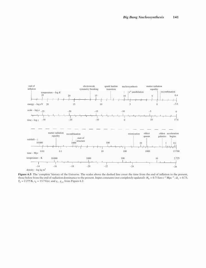
Big Bang Nucleosynthesis 141
end ofinflation
25 20
electroweaksymmetry breaking
quark hardontransition
nucleosynthesis matter radiationequality
recombinatione± annihilation
15 10 5 0.4temperature – log K
energy – log eV 20
–25
–30
10 000
10 000
0.01
matter radiationequality
recombination
start ofstructure
reionization oldestquasar
oldestgalaxies
accelerationbegins
0.1 13 700
2.725
1000
10
1000
1000
100
100
10010
10 1 0.1
redshift – z
time – Myr
temperature – K
density – log kg m3
–20 –10
–26–24–22–20–18–16–14
10 17.6
–20
15 10 5 0
–15 –10 –5
–3.6
0
0
scale – log a
time – log s
Figure 6.5 The ’complete’ history of the Universe. The scales above the dashed line cover the time from the end of inflation to the present,those below from the end of radiation dominance to the present. Input constants (not completely updated): 𝐻0 = 0.71 km s−1 Mpc−1, 𝛺
𝜆= 0.73,
𝑇0 = 2.275 K, 𝑡0 = 13.7 Gyr, and 𝑔∗, 𝑔∗𝑆 from Figure 6.2.

142 Thermal History of the Universe
6.6 Baryosynthesis and Antimatter Generation
In Equation (6.96) we noted that the ratio 𝜂 of the baryon number density 𝑁B to thephoton number density 𝑁
𝛾is very small. We shall see later that it is even two orders
of magnitude smaller.
The Ratio of Baryons to Photons. Before the baryons were formed (at about200 MeV), the conserved baryon number 𝐵 was carried by quarks. Thus the total valueof 𝐵 carried by all protons and neutrons today should equal the total value carried byall quarks. It is very surprising then that 𝜂 should be so small today, because whenthe quarks, leptons and photons were in thermal equilibrium there should have beenequal numbers of quarks and anti-quarks, leptons and anti-leptons, and the value of𝐵 was equal to the total leptonic number 𝐿,
𝑁B = 𝑁B = 𝑁L ≈ 𝑁𝛾
(6.100)
because of the 𝑈 (1)𝐵−𝐿 symmetry.
When the baryons and anti-baryons became nonrelativistic, the numbers ofbaryons and anti-baryons were reduced by annihilation, so 𝑁B decreased rapidly bythe exponential factor in the Maxwell–Boltzmann distribution [Equation (6.29)]. Thenumber density of photons 𝑁
𝛾is given by Equation (6.12) at all temperatures. Thus
the temperature dependence of 𝜂 should be
𝜂 =𝑁B
𝑁𝛾
=√
2𝜋4.808
(𝑚
𝑁
kT
)3∕2e−𝑚𝑁
∕kT. (6.101)
When the annihilation rate became slower than the expansion rate, the value of 𝜂
was frozen, and thus comparable to its value today. The freeze-out occurs at about20 MeV, when 𝜂 has reached the value
𝜂 ≃ 6.8 × 10⁻¹⁹. (6.102)
But this is a factor 9 × 10⁸ too small! Thus something must be seriously wrong withour initial condition [Equation (6.100)].
Baryon–Anti-baryon Asymmetry. The other surprising thing is that no anti-baryonsseem to have survived. At temperatures above 200 MeV, quarks and anti-quarks werein thermal equilibrium with the photons because of reactions such as Equations(6.30)–(6.32), as well as
𝛾 + 𝛾 ↔ q + q. (6.103)
These reactions conserve baryon number, so every quark produced or annihilatedis accompanied by one anti-quark produced or annihilated. Since all quarks andanti-quarks did not have time to annihilate one another, it would be reasonable toexpect equal number densities of baryons or anti-baryons today.
But we know that the Earth is only matter and not antimatter. The solar wind doesnot produce annihilations with the Earth or with the other planets, so we know that

Baryosynthesis and Antimatter Generation 143
the Solar System is matter. Since no gamma rays are produced in the interaction of thesolar wind with the local interstellar medium, we know that the interstellar medium,and hence our Galaxy, is matter. The main evidence that other galaxies are not com-posed of antimatter comes from cosmic rays. Our Galaxy contains free protons (cos-mic rays) with a known velocity spectrum very near the speed of light. A fraction ofthese particles have sufficiently high velocities to escape from the Galaxy. These pro-tons would annihilate with antimatter cosmic rays in the intergalactic medium or incollisions with antimatter galaxies if they existed, and would produce characteristicgamma rays many orders of magnitude more frequently than have been seen. Theobserved ratio is
𝑁B
𝑁B= 10−5 − 10−4
,
depending on the kinetic energy. This small number is fully consistent with all theobserved anti-protons having been produced by energetic cosmic rays in the Earth’satmosphere, and it essentially rules out the possibility that other galaxies emit cos-mic rays composed of antimatter. There are many other pieces of evidence againstantimatter, but the above arguments are the strongest.
We are then faced with two big questions. What caused the large value of 𝜂? Andwhy does the Universe not contain antimatter, anti-quarks and positrons. The onlyreasonable conclusion is that 𝑁B and 𝑁B must have started out slightly different whilethey were in thermal equilibrium, by the amount
𝑁B −𝑁B ≃ 𝜂𝑁𝛾. (6.104)
Subsequently most anti-baryons were annihilated, and the small excess 𝜂𝑁𝛾
ofbaryons is what remained. This idea is fine, but the basic problem has not beenremoved; we have only pushed it further back to earlier times, to some early BB-asymmetric phase transition.
Primeval Asymmetry Generation. Let us consider theories in which a BB-asymmetry could arise. For this three conditions must be met.
First, the theory must contain reactions violating baryon number conservation.Grand unified theories are obvious candidates for a reason we have already met inSection 6.2. We noted there that GUTs are symmetric with respect to leptons andquarks, because they are components of the same field and GUT forces do not see anydifference. Consequently, GUTs contain leptoquarks X, Y which transform quarks intoleptons. Reactions involving X, Y do explicitly violate both baryon number conserva-tion and lepton number conservation since the quarks have 𝐵 = 1
3, 𝐿
𝑖= 0, whereas lep-
tons have 𝐵 = 0, 𝐿𝑖= 1, where 𝑖 = e, 𝜇, 𝜏. The baryon and lepton numbers then change,
as for instance in the decay reactions
𝑋 → e− + d, 𝛥𝐵 = +13, 𝛥𝐿e = 1, (6.105)
𝑋 → u + u, 𝛥𝐵 = −23. (6.106)

144 Thermal History of the Universe
Second, there must be C and CP violation in the theory, as these operators changebaryons into anti-baryons and leptons into anti-leptons. If the theory were C and CPsymmetric, even the baryon-violating reactions (6.105) and (6.106) would be matchedby equally frequently occurring reactions with opposite 𝛥𝐵, so no net BB-asymmetrywould result. In fact, we want baryon production to be slightly more frequent thananti-baryon production.
Third, we must require these processes to occur out of thermal equilibrium. In ther-mal equilibrium there is no net production of baryon number, because the X-reactions(6.105) and (6.106) go as frequently in the opposite direction. Hence the propitiousmoment is the phase transition when the X-bosons are freezing out of thermal equi-librium and decay. If we consult the timetable in Section 6.2, this would happen atabout 1014 GeV: the moment for the phase transition from the GUT symmetry to itsspontaneously broken remainder.
The GUT symmetry offers a good example, which we shall make use of in thissection, but it is by no means obvious that GUT is the symmetry we need and that thephase transition takes place at GUT temperature. It is more likely that we have thebreaking of a symmetry at a lower energy, such as supersymmetry.
Leptoquark Thermodynamics. Assuming the GUT symmetry, the scenario is there-fore the following. At some energy 𝐸X = 𝑘𝑇X which is of the order of the rest massesof the leptoquark bosons X,
𝐸X ≃ 𝑀X𝑐2, (6.107)
all the X, Y vector bosons , the Higgs bosons, and the gluons are in thermal equilibriumwith the leptons and quarks. The number density of each particle species is about thesame as the photon number density, and the realations in Equation (6.100) hold.
When the age of the Universe is still young, as measured in Hubble time 𝜏H, com-pared with the mean life 𝜏X = 𝛤
−1X of the X bosons, there are no X decays and therefore
no net baryon production. The X bosons start to decay when
𝛤X ≲ 𝜏−1H = 𝐻. (6.108)
This is just like the condition in Equation (5.62) for the decoupling of neutrinos. Thedecay rate 𝛤X is proportional to the mass 𝑀X,
𝛤X = 𝛼𝑀X, (6.109)
where 𝛼 is essentially the coupling strength of the GUT interaction. It depends on thedetails of the GUT and the properties of the X boson.
We next take the temperature dependence of the expansion rate 𝐻 from Equa-tions (6.43) and (6.45). Replacing the Newtonian constant 𝐺 by its expression in termsof the Planck mass 𝑀P, as given in Equation (6.2), we find
𝐻 =√
4𝜋ℏ𝑎3𝑐
𝑔∗(𝑇 )𝑇
2
𝑀P. (6.110)

Baryosynthesis and Antimatter Generation 145
Substituting this 𝐻 and the expression in Equation (6.109) into Equation (6.108), theUniverse is out of equilibrium when
𝐴𝑀X ≲
√𝑔∗(𝑇 )
𝑇2
𝑀Pat 𝑇 = 𝑀X, (6.111)
where all the constants have been lumped into 𝐴. Solving for the temperature squared,we find
𝑇2≳
𝐴𝑀X𝑀P√𝑔∗(𝑇 )
. (6.112)
At temperature 𝑇X, the effective degrees of freedom 𝑔∗ are approximately 100. Thecondition in Equation (6.112) then gives a lower limit to the X boson mass,
𝑀X ≳ 𝐴′ 𝑀P√
𝑔∗(𝑇 )= 𝐴
′ 1.2 × 10¹⁹ GeV√10 675
≃ 𝐴′ × 1018 GeV, (6.113)
where 𝐴′ includes all constants not cited explicitly.
Thus, if the mass 𝑀X is heavier than 𝐴′ × 1018 GeV, the X bosons are stable at ener-gies above 𝑀X. Let us assume that this is the case. As the energy drops below 𝑀X,the X and X bosons start to decay, producing the net baryon number required. Theinteractions must be such that the decays really take place out of equilibrium, that is,the temperature of decoupling should be above 𝑀X. Typically, bosons decouple fromannihilation at about 𝑀X∕20, so it is not trivial to satisfy this requirement.
Let us now see how C and CP violation can be invoked to produce a net BB-asymmetry in X and X decays. The effect of the discrete operator C called charge con-jugation on a particle state is to reverse all flavours, lepton numbers and the baryonnumber. The mirror reflection in three-space is called parity transformation, and thecorresponding parity operator is denoted P. Obviously, every vector 𝒗 in a right-handedcoordinate system is transformed by P into its negative in a left-handed coordinatesystem, CP transforms left-handed leptons into right-handed antileptons.
We can limit ourselves to the case when the only decay channels are Equa-tions (6.105) and (6.106), and correspondingly for the X channels. For these chan-nels we tabulate in Table A.7 the net baryon number change 𝛥𝐵 and the 𝑖th branchingfractions 𝛤 (𝑋 → channel 𝑖)∕𝛤 (𝑋 → all channels) in terms of two unknown parameters𝑟 and 𝑟.
The baryon number produced in the decay of one pair of X,X vector bosonsweighted by the different branching fractions is then
𝛥𝐵 = 𝑟𝛥𝐵1 + (1 − 𝑟)𝛥𝐵2 + 𝑟𝛥𝐵3 + (1 − 𝑟)𝛥𝐵4 = 𝑟 − 𝑟. (6.114)
If C and CP symmetry are violated, 𝑟 and 𝑟 are different, and we obtain thedesired result 𝛥𝐵 ≠ 0. Similar arguments can be made for the production of a netlepton–anti-lepton asymmetry, but nothing is yet known about leptonic CP violation.
Suppose that the number density of X and X bosons is 𝑁X. We now want to generatea net baryon number density
𝑁B = 𝛥𝐵𝑁X ≃ 𝛥𝐵𝑁𝛾

146 Thermal History of the Universe
by the time the Universe has cooled through the phase transition at 𝑇GUT. After thatthe baryon number is absolutely conserved and further decrease in 𝑁B only followsthe expansion. However, the photons are also bosons, so their absolute number isnot conserved and the value of 𝜂 may be changing somewhat. Thus, if we want toconfront the baryon production 𝛥𝐵 required at 𝑇GUT with the present-day value of 𝜂,a more useful quantity is the baryon number per unit entropy 𝑁B∕𝑆. Recall that theentropy density of photons is
𝑠 = 1.80𝑔∗(𝑇 )𝑁𝛾(6.115)
from Equation (6.60). At temperature 𝑇GUT the effective degrees of freedom wereshown in Equation (6.46) to be 106.75 (in the standard model, not counting lepto-quark degrees of freedom), so the baryon number per unit entropy is
𝑁B
𝑆= 𝛥𝐵
1.80𝑔∗(𝑇GUT)≃ 𝛥𝐵
180. (6.116)
Clearly this ratio scales with 𝑔−1∗ (𝑇 ). Thus, to observe a present-day value of 𝜂 at about
the expected value the GUT should be chosen such that it yields
𝛥𝐵 =𝑔∗(𝑇GUT)𝑔∗(𝑇0)
𝜂 ≃ 106.753.36
𝜂 ≈ 1.9 × 10⁻⁸, (6.117)
making use of the 𝑔∗(𝑇 ) values in Equations (6.67) and (6.46). This is within the pos-sibilities of various GUTs.
One may of course object that this solution of the baryosynthesis problem is onlyspeculative, since it rests on the assumption that nature exhibits a suitable symmetry.At the beginning of this section, we warned that the GUT symmetry did not necessarilyoffer the best phase transition mechanism for baryosynthesis. The three conditionsreferred to could perhaps be met at some later phase transition. The reason why theGUT fails is to be found in the scenarios of cosmic inflation (Chapter 7). The baryonasymmetry produced at 𝑇GUT is subsequently washed out when the Universe reheatsto 𝑇GUT at the end of inflation.
The search for another mechanism has turned to the electroweak phase transitionat about 100 GeV. The ‘minimal standard model’ of electroweak interactions cannotgenerate an asymmetry but, if the correct electroweak theory could be more general.New possibilities arise if all three neutrino species oscillate and violate CP, or if oneturns to the ‘minimal supersymmetric standard model’. At the expanding interfaceof the broken symmetry phase, the baryon–anti-baryon asymmetry could be gener-ated via complex CP-violating reflections, transmissions and interference phenomenabetween fermionic excitations. Thus the existence of baryons is an indication thatphysics indeed has to go beyond the ‘minimal standard model’.
CPT Symmetry and Antigravity. A third discrete symmetry of importance is timereversal T, or symmetry under inversion of the arrow of time. This is a mirror symmetrywith respect to the time axis, just as parity was a mirror symmetry with respect to thespace axes. All physical laws of reversible processes are formulated in such a way thatthe replacement of time 𝑡 by −𝑡 has no observable effect. The particle reactions in

Baryosynthesis and Antimatter Generation 147
Section 5.3 occur at the same rate in both directions of the arrow. To show this, onestill has to compensate for differences in phase space, i.e. the bookkeeping of energyin endothermic and exothermic reactions.
Although time reversal is not very important in itself, for instance particles do notcarry a conserved quantum number related to T, it is one factor in the very importantcombined symmetry CPT. According to our most basic notions in theoretical physics,CPT symmetry must be absolute. It then follows from the fact that CP is not an abso-lute symmetry, but slightly violated, that T must be violated by an equal and oppositeamount.
In a particle reaction, CPT symmetry implies that a left-handed particle enteringthe interaction region from the 𝑥-direction is equivalent to a right-handed antiparticleleaving the region in the 𝑥-direction. One consequence of this is that particles andantiparticles must have exactly the same mass and, if they are unstable, they mustalso have exactly the same mean life.
Needless to say, many ingenious experiments have been and still are carried out totest CP violation and T violation to ever higher precision. CPT symmetry will probablybe tested when sufficient numbers of anti-hydrogen atoms have been produced, andtheir properties will be compared with those of hydrogen.
Let us assume that general relativity is CPT invariant. It certainly is so in flatspace-time even if it has not been demonstrated in curved space-time. Although Ctransforms particles into antiparticles, invariance under CPT implies that an addi-tional PT transformation is needed, too. This part changes the sign of each componentof a four-vector and odd-rank tensor, not affecting even-rank tensors. C is ineffectivebecause, contrary to electrodynamics, there is no charge in the gravitational field.
When CPT is applied even-rank (odd-rank) tensors which are PT-even (PT-odd)become CPT-odd (CPT-even). The change of sign of any d𝑥𝜇 implies that the d𝑡 ofantimatter will be reversed with respect to that of matter. Consequently the Lorentzfactor 𝛾 = d𝑡∕d𝜏 will be negative for antimatter while a matter particle has 𝛾 = 1 inits rest frame. Thus antiparticles are just particles travelling backwards in time. InEinsteins equation there are only even-rank tensors and scalars, so it is even underPT and CPT.
CPT invariance then implies that antimatter is attracted by antimatter in exactlythe same way as matter is attracted by matter, but it is not obvious what the interactionbetween matter and antimatter is. In comparison with electrodynamics, the gravita-tional field possesses no charge, but the four-momentum for a particle of mass 𝑚
𝑝𝜇 = 𝑚
d𝑥𝜇
d𝜏, (6.118)
takes the role of a charge. Recall the expression for the four-acceleration in Equa-tion (3.14)
d2𝑥𝜇
d𝜏2= −𝛤𝜇
𝜎𝜈
d𝑥𝜎
d𝜏d𝑥𝜈
d𝜏= 0. (6.119)
Under (C)PT this is even because the product of the four-momenta of two particles iseven, the product of the four-momenta of two antiparticles is even, the affine connec-tion is odd, and there is a minus-sign on the right.

148 Thermal History of the Universe
On the other hand, following the observation of Villata [6], if one of the momentarefers to a particle and the other one to an antiparticle, the momentum vector ofthe antiparticle must be (C)PT-transformed, thus acquiring a minus-sign. This thenreverses the sign of the four-acceleration so that it becomes repulsive. As he pointsout, there are two possible interpretations for the existence of antimatter. The moreconventional one is that antiparticles really exist as entities distinct from their mattercounterparts, and that they travel forward in time, as all ordinary particles. The otherinterpretation is that antiparticles do not really exist as distinct particles, but that theyare nothing else than the corresponding particles that are traveling backwards in time(BIT).
The most convincing argument in favor of the BIT interpretation is just the CPTsymmetry of physical laws, since it offers a physical explanation to the need of cou-pling C with T (and P) for describing the behavior of antimatter: if antimatter werenot traveling back in time, why should we apply the time inversion? In other words,according to the BIT interpretation, CPT is the operation that transforms events, par-ticles and fields from one time direction to the other: the role of T is obvious, sinceit inverts time intervals, P is needed to get a proper Lorentz transformation (T and Palone are improper), and C provides the needed charge reversals to see time-reversedmatter as antimatter.
Problems
1. Show that an expansion by a factor 𝑎 leaves the black-body spectrum (6.10)unchanged, except that 𝑇 decreases to 𝑇 ∕𝑎.
2. The flow of total energy received on Earth from the Sun is expressed by thesolar constant 1.36 × 10³ J m−2 s. Use Equation (6.41) to determine the surfacetemperature of the Sun,
𝑏 = 𝜆𝑇 . (6.120)
Using this temperature and the knowledge that the dominant color of the Sunis yellow with a wavelength of 𝜆 = 0.503 μm. What energy density does that flowcorrespond to?
3. A line in the spectrum of hydrogen has frequency 𝜈 = 2.5 × 10¹⁵ Hz. If this radi-ation is emitted by hydrogen on the surface of a star where the temperature is6000 K, what is the Doppler broadening [7]?
4. A spherical satellite of radius 𝑟 painted black, travels around the Sun at a distance𝑑 from the center. The Sun radiates as a black-body at a temperature of 6000 K. Ifthe Sun subtends an angle of 𝜃 radians as seen from the satellite (with 𝜃 ≪ 1), findan expression for the equilibrium temperature of the satellite in terms of 𝜃. Toproceed, calculate the energy absorbed by the satellite, and the energy radiatedper unit time [7].
5. Use the laws of conservation of energy and momentum and the equation of rela-tivistic kinematics [Equation (3.9)] to show that positronium cannot decay intoa single photon.

Baryosynthesis and Antimatter Generation 149
6. Use the equation of relativistic kinematics [Equation (3.9)] to calculate theenergy and velocity of the muon from the decay [Equation (6.51)] of a pion atrest. The neutrino can be considered massless.
7. Calculate the energy density represented by the mass of all the electrons in theUniverse at the time of photon reheating when the kinetic energy of electrons is0.2 MeV.
8. When the pions disappear below 140 MeV because of annihilation and decay,some reheating of the remaining particles occurs due to entropy conservation.Calculate the temperature-increase factor.
9. Use the equation of relativistic kinematics [Equation (3.9)] and the conserva-tion of four-momentum to calculate the energy of the photon liberated in Equa-tion (6.80), assuming that the 4He nucleus is produced at rest (i.e., 𝑣p = 𝑣t =𝑣He = 0).
10. Free nucleons are favored over deuterons down to a radiation energy of0.07 MeV. What is the ratio of photons with energies exceeding the deuteronbinding energy 2.22 MeV to the number of protons at 0.07 MeV?
11. Propose a two-stage fusion process leading to the production of 12C.
12. Gamow’s penetration factor [Equation (6.93)] gives a rough idea about the igni-tion temperatures in stellar interiors for each fusion reaction. Estimate theseunder the simplifying assumption that the burning rates during the differentperiods are inversely proportional to the time spans (given at the end of thischapter). Take the hydrogen burning temperature to be 104 K.
13. Derive a value of weak hypercharge 𝑌 = 𝐵 − 𝐿 for the X boson from the reactionsin Equations (6.72) and (6.73).
References[1] Coleman, T. S. and Roos, M. 2003 Phys. Rev. D 68, 027702.[2] Peacock, J. A. 1999 Cosmological physics. Cambridge University Press, Cambridge.[3] Kolb, E. W. and Turner, M. S. 1990 The early Universe. Addison–Wesley, Reading, MA.[4] Beringer, J. et al. 2012 Phys. Rev. D 86, Part I, 010001.[5] Burles, S., Nollett, K. M. and Turner, M. S. 2001 Astrophys. J. 552, L1.[6] Villata, M. 2011 Europhysics Letters 94, 20001 and 2012 Astrophys. Space Sci. 337, 15.[7] Gasiorowicz, S. 1979 The structure of matter. Addison–Wesley, Reading, MA.[8] Planck Collaboration: Ade, P. A. R. et al. 2014 Astron. Astrophys.; and Preprint
arXiv:1303.5076 [astro-ph.CO][9] Izotov, Y. I., Thuan T. X. and Guseva N. G. 2014, Mon. Not. R. Astron. Soc.; and Preprint
arXiv: 1408.6953 [astro-ph.CO]


7
Cosmic Inflation
The concordance FLRW Big Bang model describes a homogeneous and isotropicadiabatically expanding Universe, having a beginning of space and time with veryproblematic initial conditions: nearly infinite temperature and density, even morehomogeneous than now since inhomogeneities are unstable because of gravitation,and tend to grow with time. Where did the 1090 particles which make up the visibleUniverse come from?
Aside from such shortcomings the FLRW model has, as so far presented, beenessentially a success story. We are now going to correct that optimistic picture andpresent a remedy: cosmic inflation.
In Section 7.1 we shall discuss problems caused by the expansion of space-time: thehorizon problem related to its size at different epochs, the monopole problem associatedwith possible topological defects, and the flatness problem associated with its metric.
There are a large number of models of cosmic inflation, the simplest being theclassical or consensus slow-roll model based on a a single scalar field, which we shallstudy in Section 7.2. It is characterized by a de Sitter-like expansion, terminating witha huge entropy increase, in violation of the law of entropy conservation.
Most other models do not provide clear predictions regarding the nature of mattercreated after inflation nor the mode of exiting inflation in a vacuum that can excitethe Standard Model degrees of freedom.
In Section 7.3 we discuss the scenario of the chaotic model, which introduces abubble universe where we inhabit one bubble, totally unaware of other bubbles. Theinflationary mechanism is the same in each bubble, but different parameter valuesmay produce totally different universes. Since our bubble must be just right for us toexist in, this model is a version of the Anthropic Principle. We close this section witha discussion of the predictions of inflation.
In Section 7.4 we turn our attention to an alternative to consensus inflation, a cyclicor bouncing universe of five dimensions containing dark energy and gravity as drivingforces.
Introduction to Cosmology, Fourth Edition. Matts Roos© 2015 John Wiley & Sons, Ltd. Published 2015 by John Wiley & Sons, Ltd.

152 Cosmic Inflation
7.1 Paradoxes of the ExpansionParticle Horizons. Recall the definition of the particle horizon, Equation (2.48),which in a spatially flat metric is
𝜒ph = 𝜎ph = 𝑐∫
𝑡0
𝑡min
d𝑡𝑎(𝑡)
= 𝑐∫
0
𝑎min
d𝑎𝑎��. (7.1)
This was illustrated in Figure 2.1. In expanding Friedmann models, the particle hori-zon is finite. Let us go back to the derivation of the time dependence of the scale factor𝑎(𝑡) in Equations (5.39)–(5.41). At very early times, the mass density term in the Fried-mann Equation (5.4) dominates over the curvature term (we have also called it thevacuum-energy term),
𝑘𝑐2
𝑎2≪
8𝜋𝐺3𝜌. (7.2)
This permits us to drop the curvature term and solve for the Hubble parameter,
��
𝑎= 𝐻(𝑡) =
(8𝜋𝐺
3𝜌
)1∕2
. (7.3)
Substituting this relation into Equation (7.1) we obtain
𝜎ph = 𝑐∫
𝑎0
𝑎min
d𝑎𝑎2(��∕𝑎)
=(
3𝑐2
8𝜋𝐺
)1∕2
∫
𝑎0
𝑎min
d𝑎𝑎2√𝜌. (7.4)
In a radiation-dominated Universe, 𝜌 scales like 𝑎−4, so the integral on the right con-verges in the lower limit 𝑎min = 0, and the result is that the particle horizon is finite:
𝜎ph ∝∫
𝑎0
0
d𝑎𝑎2𝑎−2
= 𝑎0. (7.5)
Similarly, in a matter-dominated Universe, 𝜌 scales like 𝑎−3, so the integral also con-verges, now yielding
√𝑎0. Note that an observer living at a time 𝑡1 < 𝑡0 would see a
smaller particle horizon, 𝑎1 < 𝑎0, in a radiation-dominated Universe or√𝑅1 <
√𝑅0 in
a matter-dominated Universe.Suppose however, that the curvature term or a cosmological constant dominates
the Friedmann equation at some epoch. Then the conditions in Equations (5.35)and (5.36) are not fulfilled; on the contrary, we have a negative net pressure
𝑝 < −13𝜌𝑐
2. (7.6)
Substituting this into the law of energy conservation [Equation (5.24)] we find
�� < −2 ��𝑅𝜌. (7.7)
This can easily be integrated to give the 𝑅 dependence of 𝜌,
𝜌 < 𝑅−2. (7.8)

Paradoxes of the Expansion 153
Inserting this dependence into the integral on the right-hand side of Equation (7.4)we find
𝜎ph ∝∫
𝑎0
𝑎min
d𝑎
𝑎2√𝑎−2
=∫
𝑎0
𝑎min
d𝑎𝑎, (7.9)
an integral which does not converge at the limit 𝑎min = 0. Thus the particle horizon isnot finite in this case. But it is still true that an observer living at a time 𝑡1 < 𝑡0 wouldsee a particle horizon that is smaller by ln 𝑎0 − ln 𝑎1.
Horizon Problem. A consequence of the finite age 𝑡0 of the Universe is that the par-ticle horizon today is finite and larger than at any earlier time 𝑡1. Also, the spatialwidth of the past light cone has grown in proportion to the longer time perspective.Thus the spatial extent of the Universe is larger than that our past light cone enclosestoday; with time we will become causally connected with new regions as they movein across our horizon. This renders the question of the full size of the whole Uni-verse meaningless—the only meaningful size being the diameter of its horizon at agiven time.
In Chapter 6 we argued that thermal equilibrium could be established throughoutthe Universe during the radiation era because photons could traverse the whole Uni-verse and interactions could take place in a time much shorter than a Hubble time.However, there is a snag to this argument: the conditions at any space-time point canonly be influenced by events within its past light cone, and the size of the past lightcone at the time of last scattering (𝑡LSS) would appear to be far too small to allow thecurrently observable Universe to come into thermal equilibrium.
Since the time of last scattering, the particle horizon has grown with the expansionin proportion to the 2
3-power of time (actually this power law has been valid since the
beginning of matter domination at 𝑡eq, but 𝑡LSS and 𝑡eq are nearly simultaneous). Thenet effect is that the particle horizon we see today covers regions which were causallydisconnected at earlier times.
At the time of last scattering, the Universe was about 1090 times smaller than it isnow (𝑧LSS ≈ 1065), and the time perspective back to the Big Bang was only the fraction𝑡LSS∕𝑡0 ≃ 2.3 × 10⁻⁵ of our perspective. The last scattering surface is now at comov-ing radius 14 Gpc, but at the epoch of recombination it was at a 1 + 𝑧 = 1089 timesssmaller radial distance. If we assume that the Universe was radiation dominated forall the time prior to 𝑡LSS, then, from Equation (5.40), 𝑅(𝑡) ∝
√𝑡. The particle horizon
at the LSS, 𝜎ph, is obtained by substituting 𝑎(𝑡) ∝ (𝑡LSS∕𝑡)−1∕2 into Equation (2.38) andintegrating from zero time to 𝑡LSS:
𝜎ph ∝∫
𝑡LSS
0d𝑡
(𝑡LSS
𝑡
)1∕2
= 2𝑡LSS. (7.10)
It is not very critical what we call ‘zero’ time: the lower limit of the integrand hasessentially no effect even if it is chosen as late as 10−4𝑡LSS.
The event horizon at the time of last scattering, 𝜎eh, represents the extent of theUniverse we can observe today as light from the LSS (cf. Figures 2.1 and 7.1), since wecan observe no light from before the LSS. On the other hand, the particle horizon 𝜎ph

154 Cosmic Inflation
σ eh
σ ph
5 here and nowstructures in place
reionization
recombination
Big BangLast Scattering
decoupling
20
Redshift z
890
1089
1100 0
∞
Figure 7.1 A co-moving space/conformal time diagram of the Big Bang. The observer (hereand now) is at the center. The Big Bang singularity has receded to the outermost dashed circle,and the horizon scale is schematically indicated at last scattering. It corresponds to an arc ofangle 𝜃 today. Reproduced from [1] by permission of J. Silk and Macmillan Magazines Ltd.
represents the extent of the LSS that could have come into causal contact from 𝑡 = 0to 𝑡LSS. If the event horizon is larger than the particle horizon, then all the Universe wenow see (in particular the relic CMB) could not have been in causal contact by 𝑡LSS.
The event horizon 𝜎eh, is obtained by substituting 𝑎(𝑡) ∝ (𝑡LSS∕𝑡)−2∕3 from Equa-tion (5.39) into Equation (2.50) and integrating over the full epoch of matter dom-ination from 𝑡LSS to 𝑡max = 𝑡0. Assuming flat space, 𝑘 = 0, we have
𝜎eh ∝∫
𝑡0
𝑡LSS
d𝑡(𝑡LSS
𝑡
)2∕3
= 3𝑡LSS
[(𝑡0
𝑡LSS
)1∕3
− 1
]. (7.11)
Let us take 𝑡LSS = 0.35 Myr and 𝑡0 = 15 Gyr. Then the LSS particle horizon 𝜎ph is seentoday as an arc on the periphery of our particle horizon, subtending an angle
180𝜋
[𝜎ph
𝜎eh
]LSS
≃ 1.12∘. (7.12)
This is illustrated in Figure 7.1, which, needless to say, is not drawn to scale. It followsthat the temperature of the CMB radiation coming from any 1∘ arc could not have beencausally connected to the temperature on a neighboring arc, so there is no reason whythey should be equal. Yet the Universe is homogeneous and isotropic over the full 360
∘.
This problem can be avoided, as one sees from Equations (7.6)–(7.9), when the netpressure is negative, for example, when a cosmological constant dominates. In sucha case, 𝑎(𝑡) ∝ econst.⋅𝑡 [the case 𝑤 = −1 in Equation (5.38)]. If a cosmological constantdominates for a finite period, say between 𝑡1 and 𝑡2 < 𝑡LSS, then a term econst.⋅(𝑡2−𝑡1)
enters into Equation (7.10). This term can be large, allowing a reordering of horizonsto give 𝜎ph > 𝜎eh.
The age of the Universe at temperature 20 MeV was 𝑡 = 2 ms and the distance scale2ct. The amount of matter inside that horizon was only about 10−5
𝑀⊙
, which is very

Paradoxes of the Expansion 155
far from what we see today: matter is separated into galaxies of mass 1012𝑀⊙
. Thesize of present superclusters is so large that their mass must have been assembledfrom vast regions of the Universe which were outside the particle horizon at 𝑡 = 2 ms.But then they must have been formed quite recently, in contradiction to the age of thequasars and galaxies they contain. This paradox is the horizon problem.
The lesson of Equations (7.4)–(7.9) is that we can get rid of the horizon problemby choosing physical conditions where the net pressure is negative, either by havinga large curvature term or a dominating cosmological term or some large scalar fieldwhich acts as an effective cosmological term. We turn to the latter case in Section 7.2.
GUT Phase Transition. Even more serious problems emerge as we approach veryearly times. At GUT time, the temperature of the cosmic background radiation was𝑇GUT ≃ 1.2 × 1028 K, or a factor
𝑇GUT
𝑇0≃ 4.4 × 1027
greater than today. This is the factor by which the linear scale 𝑎(𝑡) has increased sincethe time 𝑡GUT. If we take the present Universe to be of size 2000ℎ−1 Mpc = 6 × 1025 m,its linear size was only 2 cm at GUT time.
Note, however, that linear size and horizon are two different things. The horizonsize depends on the time perspective back to some earlier time. Thus the particlehorizon today has increased since 𝑡GUT by almost the square of the linear scale factor,or by
𝑡0
𝑡GUT=(𝑔∗(𝑇GUT)𝑔∗(𝑇0)
)1∕2(𝑇GUT
𝑇LSS
)2(𝑇LSS
𝑇0
)3∕2
≃ 2.6 × 1054. (7.13)
At GUT time the particle horizon was only 2 × 10⁻²⁹ m. It follows that to arrive at thepresent homogeneous Universe, the homogeneity at GUT time must have extendedout to a distance 5 × 1026 times greater than the distance of causal contact! Why didthe GUT phase transition happen simultaneously in a vast number of causally discon-nected regions? Concerning even earlier times, one may ask the same question aboutthe Big Bang. Obviously, this paradox poses a serious problem to the standard BigBang model.
In all regions where the GUT phase transition was completed, several importantparameters—such as the coupling constants, the charge of the electron, and themasses of the vector bosons and Higgs bosons—obtained values which would charac-terize the present Universe. Recall that the coupling constants are functions of energy,and the same is true for particle masses. One may wonder why they obtained the samevalue in all causally disconnected regions.
The Higgs field had to take the same value everywhere, because this is uniquelydictated by what is its ground state. But one might expect that there would be domainswhere the phase transition was not completed, so that certain remnant symmetriesfroze in. The Higgs field could then settle to different values, causing some parametervalues to be different. The physics in these domains would then be different, and so

156 Cosmic Inflation
the domains would have to be separated by domain walls, which are topological defectsof space-time. Such domain walls would contain enormous amounts of energy and,in isolation, they would be indestructible. Intersecting domain walls would produceother types of topological defects such as loops or cosmic strings wiggling their waythrough the Universe. No evidence for topological defects has been found, perhapsfortunately for us, but they may still lurk outside our horizon.
Magnetic Monopoles. A particular kind of topological defect is a magneticmonopole. Ordinarily we do not expect to be able to separate the north and southpoles of a bar magnet into two independent particles. As is well known, cutting abar magnet into two produces two dipole bar magnets. Maxwell’s equations accountfor this by treating electricity and magnetism differently: there is an electric sourceterm containing the charge 𝑒, but there is no magnetic source term. Thus free elec-tric charges exist, but free magnetic charges do not. Stellar bodies may have largemagnetic fields, but no electric fields.
Paul A. M. Dirac (1902–1984) suggested in 1931 that the quantization of the elec-tron charge might be the consequence of the existence of at least one free magneticmonopole with magnetic charge
𝑔M = 12ℏcn𝑒
≃ 68.5en, (7.14)
where 𝑒 is the charge of the electron and 𝑛 is an unspecified integer. This would thenmodify Maxwell’s equations, rendering them symmetric with respect to electric andmagnetic source terms. Free magnetic monopoles would have drastic consequences,for instance destroying stellar magnetic fields.
Without going into detail about how frequently monopoles might arise during theGUT phase transition, we assume that there could arise one monopole per ten horizonvolumes
𝑁M(𝑡GUT) = 0.1 × (2 × 10−29 m)−3,
and the linear scale has grown by a factor 4.4 × 1027. Nothing could have destroyedthem except monopole–anti-monopole annihilation, so the monopole density todayshould be
𝑁M(𝑡0) ≃ 0.1 × (4.4 × 0.02 m)−3 ≃ 150 m−3. (7.15)
This is quite a substantial number compared with the proton density which is atmost 0.17 m−3. Monopoles circulating in the Galaxy would take their energy fromthe galactic magnetic field. Since the field survives, this sets a very low limit to themonopole flux called the Parker bound. Experimental searches for monopoles havenot yet become sensitive enough to test the Parker bound, but they are certainly ingross conflict with the above value of𝑁M; the present experimental upper limit to𝑁M
is 25 orders of magnitude smaller than 𝑁𝛾.
Monopoles are expected to be superheavy,
𝑚M ≳𝑚X
𝛼GUT≃ 1016 GeV ≃ 2 × 10⁻¹¹ kg. (7.16)
Paradoxes of the Expansion 157
Combining this mass with the number densities in Equations (6.76) and (7.15) thedensity parameter of monopoles becomes
𝛺M =𝑁M𝑚M
𝜌c≃ 2.8 × 10¹⁷
. (7.17)
This is in flagrant conflict with the value of the dark energy density parameter𝛺𝜆= 1 −𝛺m = 0.72 to which we sall come back later. Thus, yet another paradox. Such
a universe would be closed and its maximal lifetime would be only a fraction of theage of the present Universe, of the order of
𝑡max = 𝜋
2𝐻0
√𝛺M
≃ 40 yr. (7.18)
Monopoles have other curious properties as well. Unlike the leptons and quarks,which appear to be pointlike down to the smallest distances measured (10−19 m), themonopoles have an internal structure. All their mass is concentrated within a coreof about 10−30 m, with the consequence that the temperature in the core is of GUTscale or more. Outside that core there is a layer populated by the X leptoquark vectorbosons, and outside that at about 10−17 m there is a shell of W and Z bosons.
The monopoles are so heavy that they should accumulate in the center of starswhere they may collide with protons. Some protons may then occasionally penetratein to the GUT shell and collide with a virtual leptoquark, which transforms a d quarkinto a lepton according to the reaction
d + Xvirtual → e+. (7.19)
Thus monopoles would destroy hadronic matter at a rate much higher than their nat-ural decay rate. This would catalyze a faster disappearance of baryonic matter andyield a different timescale for the Universe.
Flatness Problem. Recall that in a spatially flat Einstein–de Sitter universe the cur-vature parameter 𝑘 vanishes and the density parameter is 𝛺 = 1. This is obvious fromEquation (5.11), where 𝑘 and 𝛺 are related by
𝛺 − 1 = 𝑘𝑐2
��2.
The current value of the total density parameter 𝛺0 is of order unity. This does notseem remarkable until one considers the extraordinary fine-tuning required: a valueof 𝛺0 close to, but not exactly, unity today implies that 𝛺0(𝑡) at earlier times musthave been close to unity with incredible precision. During the radiation era the energydensity 𝜀r is proportional to 𝑎−4. It then follows from Equation (5.4) that
��2 ∝ 𝑎−2
. (7.20)
At GUT time, the linear scale was some 1027 times smaller than today, and since mostof this change occurred during the radiation era
𝛺 − 1 ∝ 𝑎2 ≃ 10−54. (7.21)

158 Cosmic Inflation
Thus the Universe at that time must have been flat to within 54 decimal places, atotally incredible situation. If this were not so the Universe would either have reachedits maximum size within one Planck time (10−43 s), and thereafter collapsed into asingularity, or it would have dispersed into a vanishingly small energy density. Theonly natural values for 𝛺 are therefore 0, 1 or infinity, whereas to generate a universesurviving for several Gyr without a 𝛺 value of exactly unity requires an incrediblefine-tuning. It is the task of the next sections to try to explain this.
7.2 Consensus Inflation
Let us assume that the 𝑟P-sized universe then was pervaded by a homogeneous scalarclassical field 𝜙, the inflaton field, and that all points in this universe were causallyconnected. The idea with inflation is to provide a mechanism which blows up the Uni-verse so rapidly, and to such an enormous scale, that the causal connection betweenits different parts is lost, yet they are similar due to their common origin. This shouldsolve the horizon problem and dilute the monopole density to acceptable values, aswell as flatten the local fluctuations to near homogeneity.
We already have tools to achieve this. In Section 5.2 on the de Sitter cosmology wesaw that the solution to the FLRW Equation (5.57) for a constant expansion [Equa-tion (5.58)] leads to an exponentially expanding universe [Equation (5.59)]. Inflation-ary models assume that there is a moment when the inflaton domination starts andsubsequently drives the Universe into a de Sitter-like exponential expansion in whichthe temperature 𝑇 ≃ 0.
Slow-roll Inflation Slow-roll inflation is a very simple idea which could be an effec-tive representation of a variety more complicated underlying theories. It consists ofone spatially homogeneous classical scalar field 𝜙 with a minimal kinetic term and apotential 𝑉 (𝜙). It does not really matter what this field represents, here it is just anorder parameter for a phase transition.
The total inflaton energy is of the form
12��
2 + 12(∇𝜙)2 + 𝑉 (𝜙). (7.22)
The equation of motion for the classical field 𝜙 is given by the gravity model we metin Equation (5.85), now simplified with 𝑓 (𝑅,𝜙) = 1,
𝑀= 0, and with the Lagrangian
𝜙= 1
2𝑔𝜇𝜈𝜕𝜇𝜙𝜕
𝜈𝜙 − 𝑉 (𝜙). (7.23)
In addition we need the Klein–Gordon equation for the scalar field
�� + 3𝐻�� + 𝑉 ′(𝜙) = 0. (7.24)
Here the prime refers to derivation with respect to 𝜙. The only unknown function isthe potential 𝑉 (𝜙) which contains all the important physics. Friedmann’s equationbecomes
𝐻2 + 𝑘
𝑎2= 8𝜋
3𝑀2P
(12��
2 + 12(∇𝜙)2 + 𝑉 (𝜙)
). (7.25)

Consensus Inflation 159
In small-field models the field moves over a small (subPlanckian) distance. A gen-eral parametrization is the Higgs-like potential
𝑉 (𝜙) = 𝑉0[1 − (𝜙∕𝜇)𝑝] + ... (7.26)
where the dots represent higher-order terms that become important near the end ofinflation.
In large-field models the inflaton field starts at large field values and then evolves toa minimum at the origin 𝜙 = 0. The prototypical large-field model is chaotic inflationwhere a single monomial term dominates the potential
𝑉 (𝜙) = 𝜆𝑝𝜙𝑝. (7.27)
If the field is sufficiently homogeneous, we have
(∇𝜙)2 ≪ 𝑉 (𝜙), (7.28)
and the (∇𝜙)2 term in Equation (7.25) then drops out.The stress-energy tensor for a scalar field is
𝑇𝜇𝜈
= (𝜕𝜇𝜙𝜕
𝜈𝜙 − 𝑔
𝜇𝜈)𝜙, (7.29)
and, for a homogeneous field, it takes the form of a perfect fluid with energy density
𝜌 = 12��
2 + 𝑉 (𝜙),
and pressure
𝑝 = 12��
2 − 𝑉 (𝜙).
In the de Sitter limit when 𝑝 ≃ −𝜌, the potential energy of the field dominates thekinetic energy, ��2 ≪ 𝑉 (𝜙), and the speed of the expansion,𝐻 = ��∕𝑎 is large. The poten-tial energy then acts almost as a cosmological constant 8𝜋𝐺𝑉0 ≡ 𝜆. Also 𝐻 is almostconstant and the Universe expands quasi-exponentially
𝑎(𝑡) ≃ exp(∫𝐻d𝑡
)≡ 𝑒−𝑁. (7.30)
This limit is referred to as slow-roll, and 𝑁 is the number of e-folds that the Universeexpands.
Let us rewrite the Raychauduri Equation (5.6) in the form
��
𝑎= 𝐻2(1 − 𝜖), (7.31)
where the parameter 𝜖 specifies the Equation of State
𝜖 ≡32
(𝑝
𝜌+ 1
)= 4𝜋𝐺𝑐2
(��
𝐻
)2
= −dln𝐻dln𝑎
= 𝐻−1 d𝐻d𝑁
. (7.32)
The de Sitter limit 𝑝 ≃ −𝜌 is equivalent to 𝜖 → 0 and accelerated expansion 𝑎�� > 0 isequivalent to 𝜖 < 1. Inflation takes place whenever 𝜖 < 1.

160 Cosmic Inflation
If we make the further approximation that the friction term in Equation (7.24)dominates, �� ≪ 3𝐻��, the equation of motion for scalar particles is approximately
3𝐻�� + 𝑉 ′(𝜙) ≃ 0. (7.33)
Slow rolling is characterised by the two parameters
𝜂 ≡𝑚
2Planck
16𝜋
(𝑉 ′′
𝑉
)≪ 1, 𝜖 ≡
𝑚2Planck
16𝜋
(𝑉 ′
𝑉
)2
≪ 1, (7.34)
where 𝑚2Planck
= 𝑐2∕𝐺. Single-field inflation occurs when the Universe is dominated bythe inflaton field 𝜙 and obeys the slow-roll conditions in Equation (7.32). Inflationarymodels assume that there is a moment when this domination starts and subsequentlydrives the Universe into a de Sitter-like exponential expansion in which 𝑇 ≃ 0. AlanGuth in 1981 [2] named this an inflationary universe.
Graceful Exit. Clearly the cosmic inflation cannot go on forever if we want to arriveat our present slowly expanding Friedmann–Lemaitre universe. Thus there must be amechanism to halt the exponential expansion, a graceful exit. The freedom we have toarrange this is in the choice of the potential function and its temperature-dependence,𝑉 (𝜙, 𝑇 ). Inflation ends when 1
2��
2 dominates over 𝑉 (𝜙) in Friedmann’s Equation (7.25)when the inflaton field arrives at the minimum 𝜙 = 0 of the potential in Figure 7.2.The timescale for inflation is
𝐻 =√
8𝜋𝐺3
⟨𝑉0⟩ ∝√ℏ𝑐
𝑀P≃ (10−34 s)−1
. (7.35)
One may expect that 𝜙 should oscillate near this minimum, but in a rapidly expand-ing universe, the inflaton field approaches the minimum very slowly, like a ball in aviscous medium, the viscosity 𝑉 ′(𝜑) being proportional to the speed of expansion.In the expansion the scale factor 𝑎 grows so large that the third inequality follows.Equations (7.25) and (7.24) then simplify to
𝐻2 = 8𝜋
3𝑀2P
𝑉 (𝜙) (7.36)
and
3𝐻�� = −𝑉 ′(𝜑). (7.37)
There are many ways to go beyond single-field slow-roll. So far we have describedthe minimally coupled action which implies that there is no direct couplingbetween the inflaton and the metric. We could also entertain the possibility thatthe Einstein-Hilbert action is modified at high energy with 𝑓 (𝑅) terms or withnoncanonical terms 𝐹 (𝑅,𝜙) as in Equation (5.85), or that more than one field isrelevant during inflation. These subjects are advanced and beyond the scope of thepresent monograph.
Entropy. Suppose that there is a symmetry breaking phase transition from a hot𝐺GUT-symmetric phase dominated by the scalar field 𝜙 to a cooler𝐺s-symmetric phase.

Consensus Inflation 161
Inhomogeneities of the energy density increase as the Universe develops from anordered, homogeneous low-entropy state towards a high-entropy chaos characterizedby lower-grade heat. Thus the increase in entropy defines a preferred direction of time,thermal equilibrium being the state of maximum uniformity and highest entropy. Thevery fact that thermal equilibrium is achieved at some time tells us that the Universemust have originated in a state of low entropy.
As the Universe cools through the critical temperature 𝑇GUT, bubbles of the coolphase start to appear and begin to grow. If the rate of bubble nucleation is initiallysmall the Universe supercools in the hot phase, very much like a supercooled liquidwhich has a state of lowest potential energy as a solid.
The lowest curve in Figure 6.1 and the curve in Figure 7.2 illustrates the final situ-ation when the true minimum has stabilized at 𝜙0 (denoted 𝜑0 in the figures), and thepotential energy of this true vacuum is lower than in the original false vacuum:
𝑉 (𝜙0, 𝑇cool) < 𝑉 (0, 𝑇hot).
As the potential steepens, the inflaton field begins to oscillate coherently about itsvacuum state at the minimum of the potential. When the phase transition from thesupercooled hot phase to the cool phase finally occurs at 𝑇cool the latent heat storedas vacuum energy is liberated, reheating the Universe and filling it with radiation andkinetic energy of ultrarelativistic massive scalar particles with positive pressure. At thesame time other GUT fields present massify in the process of spontaneous symmetrybreaking, suddenly filling the Universe with particles of the reheating temperature 𝑇R.Precisely how this occurs is not known, but many scenarios have been proposed.
The liberated energy heats the Universe enormously, of the order of
⟨𝑉0⟩ ≃ (𝑘𝑇R)4, (7.38)
from an ambient temperature
𝑇cool ≪ 𝑇R
to 𝑇R, which is at the 𝑇GUT scale. Only at this time can one talk about a hot Big Bang.
reheatingϕendϕ
δϕ
V(ϕ)
ϕCMB
Δϕ
ϕ
Figure 7.2 Potential energy for a real scalar field 𝜙.

162 Cosmic Inflation
As long as there were no decays or annihilations of massive particles, and all otherinteractions conserve the total number of photons 𝑛
𝛾in a comoving volume is a con-
stant. Since the entropy per photon is 𝑠 ∝ 𝑇 3 the total entropy 𝑆𝐻
due to cosmicmicrowave photons of temperature 𝑇
𝑅within our current horizon 𝑑
𝐻is
𝑆𝐻
≈ 𝑇 3𝑅𝑑
3𝐻
≈(𝑇𝑅
𝐻0
)3
≈ 1088. (7.39)
the entropy per particle is suddenly increased by the very large factor
𝑍3 =
(𝑇R
𝑇cool
)3
, (7.40)
where the ratio 𝑇R∕𝑇cool is of the order of magnitude of 1029. This is a very nonadiabaticprocess.
Using estimates of the primordial density fluctuations 𝜕𝜌∕𝜌 ≈ 10−5 the energy scaleis of the order of 10−4𝑀
𝑃, so that the number of e-folds of the inflation is 𝑁 ≈ 60
or larger. There is no upper bound to 𝑁 , so it could in fact be infinite, called eternalinflation.
At the end of inflation the Universe is a hot bubble of particles and radiation inthermal equilibrium. The energy density term in Friedmann’s equations has becomedominant, and the Universe henceforth follows a Friedmann–Lemaitre type evolutionas described in Chapters 5 and 6.
The flatness problem is now solved if the part of the Universe which became ourUniverse was originally homogeneous and has expanded by the de Sitter scale factor[Equation (5.59)]
𝑎 = e𝐻𝜏 ≃ 1029, (7.41)
or 𝐻𝜏 ≃ 65. Superimposed on the homogeneity of the pre-inflationary universe therewere small perturbations in the field 𝜑 or in the vacuum energy. At the end of inflationthese give rise to density perturbations which are the seeds of later mass structuresand which can easily explain 1090 particles in the Universe.
It follows from Equations (7.33) and (7.36) that the duration of the inflation was
𝜏 ≃ 65 × 10−34 s. (7.42)
Then also the horizon problem is solved, since the initial particle horizon has beenblown up by a factor of 1029 to a size vastly larger than our present Universe. [Note thatthe realistic particle horizon is not infinite as one would obtain from Equation (7.9),because the lower limit of the integral is small but nonzero.] Consequently, all thelarge-scale structures seen today have their common origin in a microscopic part ofthe Universe long before the last scattering of radiation.
The development of this scenario is similar to Linde’s scenario shown in Figure 7.3,except that the vertical scale here grows ‘only’ to 1029.
When our bubble of space-time nucleated, it was separated from the surroundingsupercooled hot phase by domain walls. When the phase transition finally occurredthe enormous amounts of latent heat was released to these walls. The mechanismwhereby this heat was transferred to particles in the bubbles was by the collision of

Consensus Inflation 163
S
B3
B1 A1
A2
101710–3510–43
1030
10108
1
t[s]
B4
B2
Figure 7.3 Evolution of the scale𝑅 of the Universe since Planck time in (A) Friedmann modelsand (B) inflationary expansion. During the epoch B1 the Universe expands exponentially, andduring B2 the inflation ends by reheating the Universe. After the graceful exit from inflationthe Universe is radiation dominated along B3, just as in A1, following a Friedmann expansion.The sections B4 and A2 are matter-dominated epochs.
domain walls and the coalescence of bubbles. In some models knots or topologicaldefects then remained in the form of monopoles of the order of one per bubble. Thusthe inflationary model also solves the monopole problem by blowing up the size ofthe region required by one monopole. There remains no inconsistency then with thepresent observed lack of monopoles.
Consider the contracting phase of an oscillating universe. After the time 𝑡max givenby Equation (5.52) the expansion turns into contraction, and the density of mattergrows. If the age of the Universe is short enough that it contains black holes whichhave not evaporated, they will start to coalesce at an increasing rate. Thus entropycontinues to increase, so that the preferred direction of time is unchanged. Shortlybefore the Big Crunch, when the horizon has shrunk to linear size 𝐿p, all matter hasprobably been swallowed by one enormously massive black hole.
Although Guth’s classical model of cosmic inflation may seem to solve all the prob-lems of the hot Big Bang scenario in principle, it still fails because of difficulties withthe nucleation rate. If the probability of bubble formation is large, the bubbles collideand make the Universe inhomogeneous to a much higher degree than observed. Ifthe probability of bubble formation is small, then they never collide and there is noreheating in the Universe, so each bubble remains empty. Thus there is no gracefulexit from this inflationary scenario.

164 Cosmic Inflation
Perturbations. Density perturbations in the cosmological fluid of wavelength𝛬 shiftwith the scale 𝑎(𝑡) of the expansion, or what is the same, the comoving wavelengthis a constant. This is true during matter domination and radiation domination. Thecomoving horizon grows proportionally to the conformal time 𝜏 so that wavelengths𝛬 which are outside the horizon early on will later move in.
The situation was different during inflation [3]. The initial singularity is a surfaceof constant negative conformal time 𝜏 < 0. After the Big Bang when the universe wasof zero spatial size it became spatially infinite in an infinitesimal duration of time, sothe Big Bang happened simultaneously everywhere at infinite speed. During inflation𝜏 is negative, becoming less negative until 𝜏 = 0 when the expansion with 𝑎(𝑡) com-mences. Thus perturbations of wavelengths 𝛬 which were inside the horizon in aninfinitesimal duration of time after the initial singularity will move out and disappearat superhorizon scales. The shortest wavelength perturbations are those which exitedthe horizon at 𝑁 = 0 and longer ones excited earlier. Perturbations about the samesize as our horizon today exited inflation at about N = 60.
When the perturbations enter the horizon they behave as a classical field, creatingthe inhomogeneities we observe in the CMB and the large-scale distribution of matter.A problem is that the separation into a homogeneous background, that depends onlyon time, and spatially dependent perturbations, is not unique, it depends on thechoice of gauge.
Since the introduction of metrics in Chapter 2 we have been using the coordinates𝑡, 𝑥, 𝑦, 𝑧 or 𝑥0, 𝑥1, 𝑥2, 𝑥3. The spacelike hyper-surfaces of constant 𝑡 define the slicing tothe four-dimensional space-time, while the timelike worldlines of constant x define thethreading. Each spacelike threading corresponds to a homogeneous universe while theslicing is orthogonal to these universes. In the homogeneous and isotropic universewe have studied so far our choice of coordinates was natural and we did not need toconsider alternatives.
However, in a perturbed spacetime the definition of slicing and threading is notunique. Consider replacing the time coordinate 𝑡 by a perturbed time slice 𝑡 = 𝑡 +𝛿𝑡(𝑡, x). A spatially homogeneous and isotropic function is only a function of time 𝑡,as for example the energy density 𝜌(𝑡). On the new time-slice 𝑡 the energy density willnot be homogeneous, �� 𝑡 x = 𝜌(𝑡) (𝑡 x). In general relativity we need both the matterfield perturbations and the metric perturbations, so we can use the freedom of gaugetransformation to trade one for the other. In the present example we can choose thehyper-surface of constant time to coincide with the hypersurface of constant energydensity so that the real perturbations vanish, 𝛿�� = 0.
One simple choice is to fix a gauge where the nonrelativistic limit of the full per-turbed Einstein equation can be recast as a Poisson equation with a Newtonian grav-itational potential, 𝛷. The induced metric can then be written
𝑑𝑠2 = 𝑎2(𝜏)[(1 + 2𝛷)d𝜏2 − (1 − 2𝛹 )𝛿ikd𝑥𝑖d𝑥𝑘]. (7.43)
In the presence of Einstein gravity and when the spatial part of the energy-momentumtensor is diagonal one has 𝛷 = 𝛹 . Other useful gauges can be defined.
In single-field inflation we define perturbations around the homogeneous back-ground solutions for the inflaton 𝜙 and the metric 𝑔
𝜇𝜈(𝑡) by
𝜙(𝑡, x) = 𝜙(𝑡) + 𝛿𝜙(𝑡, x), 𝑔𝜇𝜈(𝑡, x) = 𝑔
𝜇𝜈(𝑡) + 𝛿𝑔
𝜇𝜈(𝑡, x). (7.44)

The Chaotic Model 165
The metric perturbations can be decomposed into scalar, vector, and tensor pertur-bations, of which the vectors can be ignored because they are not created by inflationand they decay with the expansion. The scalar perturbations are observed and the ten-sor ones will be observed as gravitational waves in the future. The ratio of tensor toscalar perturbations, denoted 𝑟, is an observable signalling gravitational waves. By theLyth bound 𝑟 correlates with the inflaton field moving over superPlanckian distanceduring inflation, provided the scalar field space is large, > 𝑀
𝑃, and if also the flatness
of the inflaton potential is controlled dynamically over a superPlanckian field range.During inflation the inflationary energy is the dominant contribution to the
stress-energy tensor of the universe so that the inflaton perturbations back-react onthe spacetime geometry.
Primordial perturbations can give rise to nonGaussianities, but in single-fieldslow-roll inflation they are expected to be small. Large nonGaussianities can only ariseif inflaton interactions are significant during inflation.
Initially all space-time regions of size 𝐻−1 would contain inhomogeneities insidetheir respective event horizons. At every instant during the inflationary de Sitter stagean observer would see himself surrounded by a black hole with event horizon 𝐻−1
(but remember that ‘black hole’ really refers to a static metric). There is an analogybetween the Hawking radiation of black holes and the temperature in an expandingde Sitter space. Black holes radiate at the Hawking temperature 𝑇H [Equation (5.83)],while an observer in de Sitter space will feel as if he is in a thermal bath of temperature𝑇dS = 𝐻∕2𝜋.
Within a time of the order of 𝐻−1 all inhomogeneities would have traversed theHubble radius. Thus they would not affect the physics inside the de Sitter universewhich would be getting increasingly homogeneous and flat. On the other hand, theHubble radius is also receding exponentially, so if we want to achieve homogeneity itmust not run away faster than the inhomogeneities.
The theory of perturbations during inflation is, however, beyond the scope of thepresent monograph. If nonGaussianities were to be observed they would be most use-ful to select between different inflationary scenarios.
7.3 The Chaotic Model
Consider the case of chaotic inflation with the potential
𝑉 (𝜙) = 12𝑚
2𝜙𝜙
2. (7.45)
The time dependence of the field is then
𝜙(𝑡) = 𝜙𝑎−𝑚𝜑𝑀P
2√
3𝜋𝑡 ≡ 𝜙
𝑎
(1 − 𝑡𝜏
), (7.46)
where 𝜏(𝜙𝑎) is the characteristic timescale of the expansion. At early times when 𝑡 ≪ 𝜏
the scalar field remains almost constant, changing only slowly from a value 𝜙𝑎≫ 𝑀
𝑃
to its ultimate value 𝜙0. The scale factor then grows quasi-exponentially as
𝑅(𝑡) = 𝑅(𝑡𝑎) exp
(Ht − 1
6𝑚
2𝜙𝑡2), (7.47)

166 Cosmic Inflation
with 𝐻 given by
𝐻 = 2√𝜋
3
𝑚𝜙
𝑀P𝜙𝑎. (7.48)
At time 𝜏, the Universe has expanded from a linear size 𝑅(𝑡𝑎) to
𝑅(𝜏) ≃ 𝑅(𝑡𝑎) exp(𝐻𝜏) = 𝑅(𝑡
𝑎) exp
(4𝜋𝜙2
𝑎
𝑀2P
). (7.49)
For instance, a universe of linear size equal to the Planck length 𝑅(𝑡𝑎) ≃ 10−35 m has
grown to
𝑅(𝜏) ≃ 𝑅(𝑡𝑎) exp
(4𝜋𝑀2
P
𝑚2𝜙
). (7.50)
For a numerical estimate we need a value for the mass 𝑚𝜙
of the inflaton. This isnot known, but we can make use of the condition that the chaotic model must be ableto form galaxies of the observed sizes. Then the scalar mass must be of the order ofmagnitude
𝑚𝜙≃ 10−6
𝑀P. (7.51)
Inserting this estimate into Equation (7.43) we obtain the completely unfathomablescale
𝑅(𝜏) ≃ 10−35+exp(4𝜋×1012) m ≃ 105.5×10¹²m. (7.52)
It is clear that all the problems of the standard Big Bang model discussed in Sec-tion 7.1 then disappear. The homogeneity, flatness and isotropy of the Universe turnout to be consequences of the inflaton field having been large enough in a region ofsize 𝑀−1
P at time 𝑡P. The inflation started in different causally connected regions ofspace-time ‘simultaneously’ to within 10−43 s, and it ended at about 10−35 s. Our partof that region was extremely small. Since the curvature term in Friedmann’s equationsdecreased exponentially, the end result is exactly as if 𝑘 had been zero to start with. Apicture of this scenario is shown in Figure 7.3.
Quantum Fluctuations. At Planck time the universe cannot have been completelyhomogeneous and isotropic because of quantum fluctuations. Across the horizon ofsize 𝑀−1
P the field may have varied by an amount
𝛥𝜑𝑎≃𝑀p. (7.53)
But in quantum mechanics we noted that at Planck time the field 𝜙 was indefiniteby 𝑀p, at least, so that there were deviations from a pure de Sitter universe. Even ifthis universe was empty, quantum field theory tells us that empty space is filled withzero-point quantum fluctuations of all kinds of physical fields, here fluctuations fromthe classical de Sitter inflaton field.
The vacuum fluctuation spectrum of the slowly rolling scalar field during theinflationary expansion turns out to be quite unlike the usual spectrum of thermal

The Chaotic Model 167
fluctuations. This can be seen if one transforms the de Sitter metric (5.60) into themetric of a Euclidean four sphere [Equation (2.28)]. Bose fields (like the inflaton)obeying a massless Klein–Gordon equation turn out to oscillate harmonically onthis sphere with period 2𝜋∕𝐻 , which is equivalent to considering quantum statis-tics at a temperature 𝑇dS = 𝐻∕2𝜋. However, the temperature in de Sitter space ishighly unusual in that the fluctuations on the four sphere are periodic in all fourdimensions [4, 5].
The fate of a bubble of space-time clearly depends on the starting value of 𝜙. Onlywhen it is large enough will inflationary expansion commence. If 𝜙 is very muchlarger than 𝑀P, Equation (7.41) shows that the rate of expansion is faster than thetimescale 𝜏,
𝐻 ≫ 2√𝜋
3𝑚𝜙≃ 2𝜏. (7.54)
Although the wavelengths of all quantum fields then grow exponentially, the change𝛥𝜙 in the value of the inflaton field itself may be small. In fact, when the physicalwavelengths have reached the size of the Hubble radius 𝐻−1, all changes in 𝜑 areimpeded by the friction 3𝐻�� in Equation (7.37), and fluctuations of size 𝛿𝜙 freeze toan average nonvanishing amplitude of
|𝛿𝜙(𝑥)| ≃ 𝐻
2𝜋. (7.55)
Consequently, the vacuum no longer appears empty and devoid of properties.Fluctuations of a length scale exceeding𝐻−1 are outside the present causal horizon
so they no longer communicate, crests and troughs in each oscillation mode remainfrozen. But at the end of inflation, the expansion during radiation and matter dom-ination starts to return these frozen fluctuations inside the horizon. With time theybecome the seeds of perturbations we now should observe in the CMB and in thedensity distribution of matter.
The quantum fluctuations remaining in the inflaton field will cause the energy to bedumped into entropy at slightly fluctuating times. Thus, the Universe will also containentropy fluctuations as seeds of later density perturbations.
Note that the quantum fluctuations amplified during inflation also lead to selfre-production and therefore do not allow inflation to end once it has started. Inflationcontinues forever leading to a metaphysical (nonverifiable) concept of eternal uni-verse and multiverse. This damages the predictive power of the theory because in thiscase ‘anything can happen and will happen an infinite number of times’.
Linde’s Bubble Universe. Since our part of the pre-inflationary universe was sosmall, it may be considered as just one bubble in a foam of bubbles having differ-ent fates. In Linde’s chaotic model each original bubble has grown in one e-foldingtime 𝜏 = 𝐻−1 to a size comprising 𝑒3 mini-universes, each of diameter 𝐻−1. In halfof these mini-universes, on average, the value of 𝜙 may be large enough for inflationto continue, and in one-half it may be too small. In the next e-folding time the samepattern is repeated. Linde has shown that in those parts of space-time where 𝜙 grows

168 Cosmic Inflation
continuously the volume of space grows by a factor
e(3−ln 2)Ht, (7.56)
whereas in the parts of space-time where 𝜙 does not decrease the volume grows bythe factor
12
e3Ht. (7.57)
Since the Hubble parameter is proportional to 𝜙, most of the physical volume mustcome from bubbles in which 𝜙 is maximal:
𝜙 ≃𝑀2P∕𝑚𝜙. (7.58)
But there must also be an exponential number of bubbles in which 𝜙 is smaller. Thosebubbles are the possible progenitors of universes of our kind. In them, 𝜙 attains finallythe value corresponding to the true minimum 𝑉 (𝜙0), and a Friedmann–Lemaitre-typeevolution takes over. Elsewhere the inflatoric growth continues forever. Thus we hap-pen to live in a universe which is a minuscule part of a steady-state eternally inflatingmeta-universe which has no end, and therefore it also has no beginning. There is sim-ply no need to turn inflation on in the first place, and the singularity at time zero hasdropped out from the theory.
During inflation, each bubble is generating new space-time to expand into, asrequired by general relativity, rather than expanding into pre-existing space-time. Inthese de Sitter space-times the bubble wall appears to an observer as a surroundingblack hole. Two such expanding bubbles are causally disconnected, so they can nei-ther collide nor coalesce. Thus the mechanism of vacuum-energy release and transferof heat to the particles created in the phase transition is not by bubble collisions as inthe classical model. Instead, the rapid oscillations of the inflaton field 𝜙 decay away byparticle production as the Universe settles in the true minimum. The potential energythen thermalizes and the Universe reheats to some temperature of the order of 𝑇GUT.
In this reheating, any baryon–anti-baryon asymmetry produced during the GUTphase transition mechanism is washed out, that is why some other phase transitionmust be sought to explain the baryon–anti-baryon asymmetry. Thus the existence ofbaryons is an indication that particle physics indeed has to go beyond the ‘minimalstandard model’.
7.4 Predictions
One consequence of the repulsive scalar field is that any two particles appear to repeleach other. This is the Hubble expansion, which is a consequence of inflation. In non-inflationary theories the Hubble expansion is merely taken for granted.
Inflationary models predict that the density of the Universe should today be verynearly critical,
𝛺0 = 1. (7.59)
This prediction is verified to within 0.3 %. Consequently, we should not only observethat there is too little luminous matter to explain the dynamical behavior of the

A Cyclic Universe 169
Universe, we also have a precise theoretical specification for how much matter thereshould be. This links dark matter to inflation.
We have already noted that the scalar inflaton field produced a spectrum of frozendensity and radiation perturbations beyond the horizon, which moved into sight whenthe expansion of the Universe decelerated. In the post-inflationary epoch when theFriedmann expansion takes over we can distinguish between two types of pertur-bations, adiabatic fluctuations, also called curvature perturbations, and isocurvaturefluctuations, also called isothermal perturbations. In the first case, the perturbationsin the local number density, 𝛿m ≡ 𝛿𝜌m∕𝜌m, of each species of matter—baryons, leptons,neutrinos, dark matter—is the same. In particular, these perturbations are coupled tothose of radiation, 𝛿r ≡ 𝛿𝜌r∕𝜌r, so that 4𝛿m = 3𝛿r [from Equation (6.39)]. By the princi-ple of covariance, perturbations in the energy-momentum tensor imply simultaneousperturbations in energy density and pressure, and by the equivalence principle, vari-ations in the energy-momentum tensor are equivalent to variations in the curvature.Curvature perturbations can have been produced early as irregularities in the met-ric, and they can then have been blown up by inflation far beyond the Hubble radius.Thus adiabatic perturbations are a natural consequence of cosmic inflation. In con-trast, inflation does not predict any isocurvature perturbations.
Let us write the power spectrum of density perturbations in the form
𝑃 (𝑘) ∝ 𝑘𝑛s , (7.60)
where 𝑛s is the scalar spectral index. Inflationary models predict that the primordialfluctuations have an equal amplitude on all scales, an almost scale-invariant powerspectrum as the matter fluctuations cross the Hubble radius, and are Gaussian. This isthe Harrison–Zel’dovich spectrum for which 𝑛s = 1 (𝑛s = 0 would correspond to whitenoise).
A further prediction of inflationary models is that tensor fluctuations in the space-time metric, satisfying a massless Klein–Gordon equation, have a nearly scale-invariant spectrum of the form in Equation (7.59) with tensor spectral index 𝑛t, justlike scalar density perturbations, but independently of them. The ratio 𝑟 = 𝑛t∕𝑛s is noweagerly measured by several teams.
The above predictions are generic for a majority if inflation models which differ indetails. Inflation as such cannot be either proved or disproved, but specific theoriescan be and will be ruled out by these observations.
7.5 A Cyclic Universe
As we have seen, ‘consensus’ inflation by a single inflaton field solves the problemsdescribed in Section 7.1. But in the minds of some people it does so at a very highprice. It does not explain the beginning of space and time, it does not predict thefuture of the Universe, or it sweeps these fundamental questions under the carpet ofthe anthropic principle. It invokes several unproven ingredients, such as a scalar fieldand a scalar potential, suitably chosen for the field to slow-roll down the potentialwhile its kinetic energy is negligible, and such that it comes to a graceful exit where
170 Cosmic Inflation
ordinary matter and radiation are created by oscillations in the potential well, or byentropy generation during a second slow-roll phase of an equally arbitrary dark energyfield. Clearly, any viable alternative to single-field inflation must also be able to solvethe problems in Section 7.1, and it should not contain more arbitrary elements thandoes single-field inflation—multiple scalar fields have more freedom but also morearbitrariness.
In the radiation-dominated Universe, the source of energy of photons and otherparticles is a phase transition or a particle decay or an annihilation reaction, manyof these sources producing monoenergetic particles. Thus the energy spectrum pro-duced at the source is very nonuniform and nonrandom, containing sharp spectrallines ‘ordered’ by the type of reaction. Such a spectrum corresponds to low entropy.Subsequent scattering collisions will redistribute the energy more randomly and ulti-mately degrade it to high-entropy heat. Thermal equilibrium is the state of maximumuniformity and highest entropy. The very fact that thermal equilibrium is achieved atsome time tells us that the Universe must have originated in a state of low entropy.
In the transition from radiation domination to matter domination no entropy islost. We have seen the crucial effect of photon reheating due to entropy conservationin the decoupling of the electrons. As the Universe expands and the wavelengths of theCMB photons grow, the available energy is continuously converted into lower-gradeheat, thus increasing entropy. This thermodynamic argument defines a preferred direc-tion of time.
When the cooling matter starts to cluster and contract under gravity, a new phasestarts. We have seen that the Friedmann–Lemaitre equations dictate instability, thelumpiness of matter increases with the Universe developing from an ordered, homo-geneous state towards chaos. It may seem that contracting gas clouds represent higheruniformity than matter clustered into stars and galaxies. If the only form of energywere thermal, this would indeed be so. It would then be highly improbable to find a gascloud squeezed into a small volume if nothing hinders it from filling a large volume.However, the attractive nature of gravity seemingly reverses this logic: the cloud gainsenormously in entropy by contracting. Thus the preferred direction of time as definedby the direction of increasing entropy is unchanged during the matter-dominated era.
The same trend continues in the evolution of stars. Young suns burn their fuelthrough a chain of fusion reactions in which energetic photons are liberated and heav-ier nuclei are produced. As the photons diffuse in the stellar matter, they ultimatelyconvert their energy into a large number of low-energy photons and heat, therebyincreasing entropy. Old suns may be extended low-density, high-entropy red giants orwhite dwarfs, without enveloping matter which loses mass by various processes. Inthe process of supernova explosion entropy grows enormously.
Consider the contracting phase of an oscillating universe. After the time 𝑡max givenby Equation (5.52) the expansion turns into contraction, and the density of mattergrows. If the age of the Universe is short enough that it contains black holes whichhave not evaporated, they will start to coalesce at an increasing rate. Thus entropycontinues to increase, so that the preferred direction of time is unchanged. Shortlybefore the Big Crunch, when the horizon has shrunk to linear size 𝐿p, all matter hasprobably been swallowed by one enormously massive black hole.

A Cyclic Universe 171
Early attempts to build models with cyclically reoccurring expansion and contrac-tion were plagued by the problem, that the entropy density would rise from cycle tocycle. The length of cycles must then increase steadily. But, in retrospect, there mustthen have been a first cycle a finite time ago, thus a beginning of time: precisely whatthe cyclic model was conceived to avoid.
A cyclic model which solves the entropy problem and which appears as successfulas the ‘consensus’ inflationary model has been proposed by Steinhardt and Turok [6].
The model is described qualitatively in Figure 7.4, which depicts a potential 𝑉 (𝜙),function of a scalar field 𝜑. Unlike the inflaton field, 𝜙 does not cause an inflationaryexpansion of space-time. Following the arguments of Steinhardt and Turok the uni-verse is assumed to be a five-dimensional bulk, where our physical world with all itsobservable particles is located on a four-dimensional brane separated from anotherbrane by a microscopic gap (or rather “Planckoscopic”). Matter on the other brane canonly interact with our world gravitationally, but not through strong or electromagneticinteractions. Such matter is therefore dark, we cannot detect it in our laboratories.
The potential 𝑉 (𝜙) describes a force between the two branes, and 𝜙 is a moduli fieldthat describes the interbrane separation. When the two branes are far apart this forceis very weak, the branes are stretched to the point where they are flat and parallel, andwe experience this as the present slow cosmic acceleration (phase 1 in Figure 7.4), thesituation where we are now. During this phase the potential energy of the scalar fielddominates over the kinetic energy of the scalar field so that dark energy drives theexpansion.
While 𝜙 decreases toward phase 2, the potential slow-rolls down the weakly slopingpositive potential and the branes draw together. At point 3 in Figure 7.4 the potential
V(φ)
26Big
5
4Vcrunch
3
1V0
φBang
Figure 7.4 Schematic view of the potential 𝑉 (𝜙) as a function of the field 𝜙 for cyclic modelsin a five-dimensional universe. The numbered sequence of phases is described in the text.

172 Cosmic Inflation
has decreased to the point where 𝑉 (𝜙) = 12𝜙2 where the field crosses zero potential,
the total energy density is zero and the Hubble expansion halts. As the branes drawcloser together, the potential energy decreases from positive to negative values andthe universe switches from expansion to a rapid contraction with equation of state𝑤 ≫ 1, towards a minimum at point 4 in Figure 7.4. The spatial contraction occurs inthe extra dimension 𝜙, rather than in our three dimensions.
As the scalar field rolls down into this minimum (phase 4), it picks up speed onthe way and causes a Hubble blueshift of the scalar field kinetic energy. With thisspeed the field just continues beyond the minimum, climbs out of it on the other sideand continues towards the bounce at negative infinity in a finite time. the potentialdisappearing exponentially. In the approach towards 𝜙 = −∞, the scale factor 𝑎(𝑡) goesto zero (phase 5), but the coupling of the scalar field to radiation and matter conspiresin such a way as to keep the temperature and the energy density finite. Space does notdisappear completely since this scenario takes place in a five-dimensional space-time,and 𝑎(𝑡) has to be interpreted as the effective scale factor on the brane.
Each cycle ends and begins with a crunch turning into a bang at the field value𝜙 = −∞. The bang is a turn-around or bounce from the pre-existing contracting phasewith a decreasing field. At the bounce, the branes collide and this is the big bang ofa new cycle. After the branes bounce apart there immediately follows an expandingphase and an acceleration of the field towards positive values (phase 6 in Figure 7.4),when matter and radiation are created at large but finite temperature from the kineticenergy of the field.
This phase is quite similar to the corresponding post-inflationary epoch in the con-ventional inflationary scenario, and therefore the predictions are the same. But, unlikethe conventional model, here a subdominant dark energy field is required. Duringradiation and matter domination the scalar dark energy field is effectively frozen inplace by the Hubble redshift of its kinetic energy and the branes slow down to essen-tially a halt. The potential energy of this field starts to dominate only when radiationand matter energy densities have been sufficiently diluted by the expansion; then aslow cosmic acceleration commences (phase 1).
The heat from the collision dominates the universe for a few billion years, but even-tually, on the way from phase 6 to phase 1, it is diluted enough that the positive inter-brane potential energy density dominates. This acts as a source of dark energy thatcauses the expansion of the branes to accelerate. Although the acceleration due todark energy is very slow, causing the Universe to double in size every 15 billion yearsor so, compared with the enormous expansion in Equation (7.45) during 10−35 s, thisis enough to empty the Universe of its matter and radiation. The matter, radiation,and large scale structure dilute away over the next trillion years or so, and the branesbecome nearly perfect vacua at the end of each cycle (at phase 1), preparing the wayfor a new cycle of identical duration.
The homogeneity and flatness of the Universe and the density perturbationsare established during long periods of ultra-slow accelerated expansion, and theconditions are set up during the negative time prior to a bang. In contrast, standardinflationary theories have very little time to set up large-scale conditions, only about10−35 s until the inflationary fluctuations have been amplified and frozen in, at a length

A Cyclic Universe 173
scale of 10−25cm. In the cyclic Universe, the fluctuations can be generated a fractionof a second before the bang when their length scale is thousands of kilometres.
The entropy created in one cycle is expanded and exponentially diluted to near zerodensity after the dark energy dominated phase, but the entropy does not increase againin the contracting phase. The reason is that the branes themselves do not contract,only the extra dimension contracts. The total entropy on the branes and the numberof black holes increase from cycle to cycle, and increase per comoving volume on ourbrane as well. In the vicinity of the black holes, there is no cycling due to their stronggravitational field. Black holes formed during one cycle will therefore survive to thenext cycle, acting as defects in an otherwise nearly uniform universe.
The kinetic energy and the physical entropy density during each cycle are fed notonly by the interbrane force, but also by gravity which supplies extra energy duringthe contraction phase. This kinetic energy of the branes is converted partially intomatter and radiation and blue-shifted by the gravity.
All of this is very speculative, but so is consensus inflation, too. Fortunately, the dif-ferent models make different testable predictions, notably for gravitational radiation.A certain discovery of gravitational radiation testified by tensor perturbations in theCMB would support consensus inflation.
Problems
1. Derive Equation (7.37).
2. Derive 𝜙(𝑡) for a potential 𝑉 (𝜙) = 14𝜆𝜙4.
3. Suppose that the scalar field averaged over the Hubble radius 𝐻−1 fluctuatesby an amount 𝜓 . The field gradient in this fluctuation is ∇𝜓 = 𝐻𝜓 and the gra-dient energy density is 𝐻2𝜓2. What is the energy of this fluctuation integratedover the Hubble volume? Use the timescale 𝐻−1 for the fluctuation to changeacross the volume, and the uncertainty principle to derive the minimum valueof the energy. This is the amount by which the fluctuation has stretched in oneexpansion time [7].
4. Material observed now at redshift 𝑧 = 1 is at present distance𝐻−10 . The recession
velocity of an object at coordinate distance 𝑥 is ��𝑥. Show that the recessionvelocity at the end of inflation is
��𝑥 =𝐻0𝑅0𝑥𝑧r√
𝑧eq, (7.61)
where 𝑧r is the redshift at the end of inflation. Compute this velocity. The densitycontrast has grown by the factor 𝑧2
r∕𝑧eq. What value did it have at the end ofinflation since it is now 𝛿 ≈ 10−4 at the Hubble radius [7]?
5. Show that in an exponentially expanding universe (𝑞 = −1) the Hubble sphereis stationary. Show that it constitutes an event horizon in the sense that eventsbeyond it will never be observable. Show that in this universe there is no particlehorizon [8].

174 Cosmic Inflation
6. Show that the number of e-foldings of inflation in the 𝑉 (𝜙) = −𝜆𝜙4 model is oforder
𝑁 ≈ 𝐻2
𝜆𝜙2𝑖
from the time at which the field has the value 𝜙𝑖to the end of inflation (𝜙 ≪ 𝜙
𝑖).
Hence show that the density perturbations in this model are of order(𝛿𝜌
𝜌
)𝐻
≈√𝜆𝑁3. (7.62)
Deduce that 𝜆 < 10−14 is required if the fluctuations are to be compatible withthe CMB. This of course amounts to the fine-tuning that inflation is supposed toavoid [8].
References[1] Kaiser, N. and Silk, J. 1986 Nature 324, 529.[2] Guth, A. H. 1981 Phys. Rev. D 23, 347.[3] Kenney, W. H. 2009 TASI Lectures on Inflation, Boulder and preprint arXiv: 0902.1529
astro-ph.CO.[4] Linde, A. D. 1990 Particle physics and inflationary cosmology. Harwood Academic
Publishers, London.[5] Linde, A. D. 2002 Inflationary cosmology and creation of matter in the Universe. In Modern
cosmology (ed. S. Bonometto, V. Gorini and U. Moschella). Institute of Physics Publishing,Bristol.
[6] Steinhardt, P. J. and Turok, N. 2002 Science 296, 1496; 2005 New Astron. Rev. 49, 43.[7] Peebles, P. J. E. 1993 Principles of physical cosmology. Princeton University Press,
Princeton, NJ.[8] Raine, D. J. and Thomas, E. G. 2001 An introduction to the science of cosmology. Institute
of Physics Publishing, Bristol.

8
Cosmic MicrowaveBackground
In this chapter we shall meet several important observational discoveries. The cosmicmicrowave background (CMB), which is a consequence of the hot Big Bang and thefollowing radiation-dominated epoch, was discovered in 1964. We discuss this discov-ery in Section 8.1.
The hot Big Bang also predicts that the CMB radiation should have a blackbodyspectrum. Inflation predicts that the mean temperature of the CMB should exhibitminute perturbations across the sky. These predictions were verified by a 1990 satelliteexperiment, the Cosmic Background Explorer (COBE). The COBE observations veri-fied the existence of a nearly scale-invariant spectrum of primordial fluctuations onangular scales larger than 7∘. Many experiments have since then extended the range,in particular the Wilkinson Microwave Anisotropy Probe WMAP. Most recently thethird-generation space mission Planck has made observations of temperature andpolarization anisotropies with much improved precision and statistics at differentangular scales. These measurements will be discussed in the rest of this chapter.
In Section 8.2 we shall discuss the method of analyzing the temperature per-turbations which are expected to be associated with the even smaller polarizationvariations, due to Thomson scattering at the LSS. These were first observed by theground-based Degree Angular Scale Interferometer (DASI) in late 2002 and by in early2003. We discuss this in Section 8.3.
The CMB contains a wealth of information about the dynamical parameters ofthe Universe and on specific features of the theoretical models: general relativity, thestandard FLRW cosmology versus other cosmologies, all versions of inflation andits alternatives, dark matter, dark energy and so on. In Section 8.4 we establish theparameters, how they are related to each other, what observational values they haveand what information they give about possible cosmological models.
Introduction to Cosmology, Fourth Edition. Matts Roos© 2015 John Wiley & Sons, Ltd. Published 2015 by John Wiley & Sons, Ltd.

176 Cosmic Microwave Background
8.1 The CMB TemperaturePredictions. In 1948, Georg Gamow (1904–1968), Ralph Alpher and Robert Hermancalculated the temperature at that time of the primordial blackbody radiation whichstarted free streaming at the LSS. They found that the CMB should still exist today,but that it would have cooled in the process of expansion to the very low temperatureof 𝑇0 ≈ 5 K. This corresponds to a photon wavelength of
𝜆 = hc𝑘𝑇0
= 2.9 × 10⁻³ m. (8.1)
This is in the microwave range of radio waves (see Table A.3). (The term ‘microwave’is actually a misnomer, since it does not refer to micrometer wavelengths, but ratherto centimeters.)
We can now redo their calculation, using some hindsight. Let us first recall fromEquations (5.39) and (5.40) that the expansion rate changed at the moment whenradiation and matter contributed equally to the energy density. For our calculationwe need to know this equality time, 𝑡eq, and the temperature 𝑇eq. The radiation energydensity is given by Equation (6.41):
𝜀r = (𝑔𝛾+ 3𝑔
𝜈)12𝑎𝑇
4eq. (8.2)
The energy density of matter at time 𝑇eq is given by Equation (6.24), except that theelectron (e− and e+) energy needs to be averaged over the spectrum [Equation (6.28)].We could in principle solve for 𝑇eq by equating the radiation and matter densities,
𝜀r(𝑇eq) = 𝜌m(𝑇eq). (8.3)
We shall defer solving this to Section 8.4.The transition epoch happens to be close to the recombination time [𝑧rec in redshift,
see Equation (6.70)] and the LSS [𝑧LSS in redshift, see Equation (6.71)]. With theirvalues for 𝑡eq, 𝑇eq and 𝑡0 and Equation (5.39), Gamow, Alpher and Herman obtained aprediction for the present temperature of the CMB:
𝑇0 = 𝑇eq
(𝑡eq
𝑡0
) 2∕3
= 2.45 K. (8.4)
This is very close to the present-day observed value, as we shall see.
Discovery. Nobody paid much attention to the prediction of Gamov et al., becausethe Big Bang theory was generally considered wildly speculative, and detection of thepredicted radiation was far beyond the technical capabilities existing at that time. Inparticular, their prediction was not known to Arno Penzias and Robert Wilson who,in 1964, were testing a sensitive antenna intended for satellite communication. Theywanted to calibrate it in an environment free of all radiation, so they chose a wave-length of 𝜆 = 0.0735 m in the relatively quiet window between the known emissionfrom the Galaxy at longer wavelengths and the emission at shorter wavelengths fromthe Earth’s atmosphere. They also directed the antenna high above the galactic plane,where scattered radiation from the Galaxy would be minimal.

The CMB Temperature 177
To their consternation and annoyance they found a constant low level of back-ground noise in every direction. This radiation did not seem to originate from distantgalaxies, because in that case they would have seen an intensity peak in the directionof the nearby M31 galaxy in Andromeda. It could also not have originated in Earth’satmosphere, because such an effect would have varied with the altitude above thehorizon as a function of the thickness of the atmosphere.
Thus Penzias and Wilson suspected technical problems with the antenna (in whicha couple of pigeons turned out to be roosting) or with the electronics. All searchesfailing, they finally concluded, correctly, that the Universe was uniformly filled withan ‘excess’ radiation corresponding to a blackbody temperature of 3.5 K, and that thisradiation was isotropic and unpolarized within their measurement precision.
At Princeton University, a group of physicists led by Robert Dicke (1916–1997) hadat that time independently arrived at the conclusion of Gamow and collaborators, andthey were preparing to measure the CMB radiation when they heard of the remark-able 3.5 K ‘excess’ radiation. The results of Penzias and Wilson’s measurements wereimmediately understood and they were subsequently published (in 1965) jointly withan article by Dicke and collaborators which explained the cosmological implications.The full story is told by Peebles [1], who was a student of Dicke at that time. Penziasand Wilson (but not Gamow or Dicke) were subsequently awarded the Nobel prize in1978 for this discovery.
This evidence for the 15-Gyr-old echo of the Big Bang counts as the most importantdiscovery in cosmology since Hubble’s law. In contrast to all radiation from astro-nomical bodies, which is generally hotter, and which has been emitted much later,the CMB has existed since the era of radiation domination. It is hard to understandhow the CMB could have arisen without the cosmic material having once been highlycompressed and exceedingly hot. There is no known mechanism at any time afterdecoupling that could have produced a blackbody spectrum in the microwave range,because the Universe is transparent to radio waves.
Spectrum. In principle, one intensity measurement at an arbitrary wavelength ofthe blackbody spectrum (6.10) is sufficient to determine its temperature, 𝑇 , becausethis is the only free parameter. On the other hand, one needs measurements at differ-ent wavelengths to establish that the spectrum is indeed blackbody.
It is easy to see that a spectrum which was blackbody at time 𝑡 with temperature 𝑇will still be blackbody at time 𝑡′ when the temperature has scaled to
𝑇′ = 𝑇 𝑎(𝑡)
𝑎(𝑡′). (8.5)
This is so because, in the absence of creation or annihilation processes, the number ofphotons, 𝑛
𝛾𝑎3(𝑡), is conserved. Thus the number density d𝑛
𝛾(𝜈) in the frequency interval
(𝜈, 𝜈 + d𝜈) at time 𝑡 transforms into the number density at time 𝑡′,
d𝑛′𝛾(𝜈′) =
[𝑎(𝑡)𝑎(𝑡′)
] 3
d𝑛𝛾(𝜈). (8.6)

178 Cosmic Microwave Background
Making use of Equations (6.10) and (8.5), the distribution at time 𝑡′ becomes
d𝑛′𝛾(𝜈′) = 8𝜋
3𝑐3
d𝜈′3
eℎ𝜈′∕𝑘𝑇 ′ − 1, (8.7)
which is precisely the blackbody spectrum at temperature 𝑇 ′.Although several accurate experiments since Penzias and Wilson have confirmed
the temperature to be near 3 K by measurements at different wavelengths, the conclu-sive demonstration that the spectrum is indeed also blackbody in the region maskedby radiation from the Earth’s atmosphere was first made by a dedicated instrument,the Far Infrared Absolute Spectrophotometer (FIRAS) aboard the COBE satellitelaunched in 1989 [2]. The present value of the photon temperature, 𝑇0, is from mea-surements in 2009,
𝑇0 = 2.7255 ± 0.0006 K. (8.8)
The spectrum reported by the COBE team in 1993 [3] matches exactly the the-oretical prediction for blackbody radiation remaining from the hot Big Bang. Themeasurement errors on each of the 34 wavelength positions have not been added tothe theoretical blackbody curve because they could not be distinguished It is worthnoting that such a pure blackbody spectrum had never been observed in laboratoryexperiments. All theories that attempt to explain the origin of large-scale structureseen in the Universe today must conform to the constraints imposed by these COBEmeasurements.
The vertical scale in Figure 8.1 gives the intensity 𝐼(1∕𝜆) of the radiation, that is, thepower per unit inverse wavelength interval arriving per unit area at the observer from
1.2
1.0 Theory and observation agree
Inte
nsity
, 10–
4 erg
s/cm
2 sr
sec
cm–1
0.8
0.6
0.4
0.2
0.00 5 10
Waves/cm
15 20
Figure 8.1 The theoretical blackbody spectrum from Equation (6.13). From D. J. Fixsen,E. S. Cheng, J. M. Gales, J. C. Mather, R. A. Shafer, and E. L. Wright, The Cosmic MicrowaveBackground Spectrum from the Full COBE* FIRAS Data Set. Astrophys. J., 473, 576, published20 December ©1996. AAS. Reproduced with permission.

The CMB Temperature 179
one steradian of sky. In SI units this is 10−9 J m−1 sr−1 s−1. This quantity is equivalentto the intensity per unit frequency interval, 𝐼(𝜈). One can transform from d𝜆 to d𝜈 bynoting that 𝐼(𝜈) d𝜈 = 𝐼(𝜆) d𝜆, from which
𝐼(𝜆) = 𝜈2
𝑐𝐼(𝜈). (8.9)
The relation between energy density 𝜀r and total intensity, integrated over the spec-trum, is
𝜀r =4𝜋𝑐 ∫
𝐼(𝜈) d𝜈. (8.10)
Energy and Entropy Density. Given the precise value of 𝑇0 in Equation (8.8), onecan determine several important quantities. From Equation (6.41) one can calculatethe present energy density of radiation
𝜀𝑟,0 = 1
2𝑔∗𝑎S𝑇
40 = 2.606 × 10⁵ eV m−3
. (8.11)
The corresponding density parameter then has the value
𝛺r =𝜀𝑟,0
𝜌c= 2.473 × 10⁻⁵ h−2
, (8.12)
using the value of 𝜌c from Equation (1.31) and the compromise value𝐻0 = 0.71. Obvi-ously, the radiation energy is very small today and far from the value 𝛺0 = 1 requiredto close the Universe.
The present value of the entropy density is
𝑠 = 43
𝜀𝑟,0
kT= 4
3𝑔∗S
2𝑎S𝑇
4
kT= 2.890 × 10⁹ m−3
. (8.13)
Recall [from the text immediately after Equation (6.67)] that the (𝑇𝜈∕𝑇 ) dependence
of 𝑔∗S is a power of three rather than a power of four, so the factor ( 411)4∕3 becomes
just 411
and 𝑔∗S becomes 3.91.The present number density of CMB photons is given directly by Equation (6.12):
𝑁𝛾= 𝜁(3) 2
𝜋2
(kT𝑐ℏ
) 3
= 4.11 × 10⁸ photons m−3. (8.14)
Neutrino Number Density. Now that we know 𝑇0 and𝑁𝛾
we can obtain the neutrinotemperature 𝑇
𝜈= 1.949 K from Equation (6.65) and the neutrino number density per
neutrino species from Equation (6.66),
𝑁𝜈= 3
11𝑁𝛾= 1.12 × 10⁸ neutrinos m−3
. (8.15)
For three species of relic neutrinos with average mass ⟨𝑚𝜈⟩, Equation (6.68) can be
used to cast the density parameter in the form
𝛺𝜈=
3⟨𝑚𝜈⟩
94.0ℎ2 eV. (8.16)

180 Cosmic Microwave Background
8.2 Temperature AnisotropiesDipole Anisotropy. The temperature measurement of Penzias and Wilson’s antennawas not very precise by today’s standards. Their conclusion about the isotropy of theCMB was based on an accuracy of only 1.0 K. When the measurements improved overthe years it was found that the CMB exhibited a dipole anisotropy. The temperaturevaries minutely over the sky in such a way that it is maximally blueshifted in onedirection (call it 𝛼) and maximally redshifted in the opposite direction (𝛼 + 180∘). Ina direction 𝛼 + 𝜃 it is
𝑇 (𝜃) = 𝑇 (𝛼) (1 + 𝜈 cos 𝜃), (8.17)
where 𝜈 is the amplitude of the dipole anisotropy. Although this shift is small, only𝜈𝑇 (𝛼) ≈ 3.35 mK, it was measured with an accuracy better than 1% by the DifferentialMicrowave Radiometer (DMR) instrument on board the COBE satellite [4].
At the end of Chapter 5 we concluded that the hot Big Bang cosmology predictedthat the CMB should be essentially isotropic, since it originated in the LSS, whichhas now receded to a redshift of 𝑧 ≃ 1080 in all directions. Note that the most distantastronomical objects known have redshifts of about 𝑧 = 7. Their distance in time tothe LSS is actually much closer than their distance to us.
In the standard model the expansion is spherically symmetric, so it is quite clearthat the dipole anisotropy cannot be of cosmological origin. Rather, it is well explainedby our motion ‘against’ the radiation in the direction of maximal blueshift with relativevelocity 𝜈.
Thus there is a frame in which the CMB is isotropic—not a rest frame, since radia-tion cannot be at rest. This frame is then comoving with the expansion of the Universe.We referred to it in Section 2.2, where we noted that, to a fundamental observer atrest in the comoving frame, the Universe must appear isotropic if it is homogeneous.Although general relativity was constructed to be explicitly frame independent, thecomoving frame in which the CMB is isotropic is observationally convenient. Thefundamental observer is at position B in Figure 8.2.
The interpretation today is that not only does the Earth move around the Sun, andthe Solar System participates in the rotation of the Galaxy, but also the Galaxy movesrelative to our Local Galaxy Group, which in turn is falling towards a center behind theHydra–Centaurus supercluster in the constellation Virgo. From the observation thatour motion relative to the CMB is 369 ± 0.9 km s−1, these velocity vectors add up to apeculiar motion of the Galaxy of about 550 km s−1, and a peculiar motion of the LocalGroup of about 630 km s−1 [5]. Thus the dipole anisotropy seen by the Earth-basedobserver A in Figure 8.1 tells us that we and the Local Group are part of a larger,gravitationally bound system.
Multipole Analysis. Temperature fluctuations around a mean temperature 𝑇0 in adirection 𝛼 on the sky can be analyzed in terms of the autocorrelation function 𝐶(𝜃),which measures the product of temperatures in two directions m,n separated by anangle 𝜃 and averaged over all directions 𝛼,
𝐶(𝜃) =⟨𝛿𝑇 (m)𝑇0
𝛿𝑇 (n)𝑇0
⟩, m ⋅ n = cos 𝜃. (8.18)

Temperature Anisotropies 181
A
B
Figure 8.2 The observer A in the solar rest frame sees the CMB to have dipole anisotropy—thelength of the radial lines illustrate the CMB intensity—because he is moving in the directionof the arrow. The fundamental observer at position B has removed the anisotropy.
For small angles (𝜃) the temperature autocorrelation function can be expressed as asum of Legendre polynomials 𝑃𝓁(𝜃) of order 𝓁, the wavenumber, with coefficients orpowers 𝑎2
𝓁,
𝐶(𝜃) = 14𝜋
∞∑𝓁=2
𝑎2𝓁(2𝓁 + 1)𝑃𝓁(cos 𝜃). (8.19)
All analyses start with the quadrupole mode 𝓁 = 2 because the 𝓁 = 0 monopole modeis just the mean temperature over the observed part of the sky, and the 𝓁 = 1 mode isthe dipole anisotropy. As a rule of thumb, higher multipoles correspond to fluctuationson angular scales
𝜃 ≃ 60∘𝓁.
In the analysis, the powers 𝑎2𝓁 are adjusted to give a best fit of 𝐶(𝜃) to the observed
temperature. The resulting distribution of 𝑎2𝓁 values versus 𝓁 is called the power
spectrum of the fluctuations. The higher the angular resolution, the more terms of

182 Cosmic Microwave Background
high 𝓁 must be included. Anisotropies on the largest angular scales corresponding toquadrupoles are manifestations of truly primordial gravitational structures.
For the analysis of temperature perturbations over large angles, the Legendre poly-nomial expansion in Equation (8.19) will not do; one has to use tensor sphericalharmonics. The temperature 𝑇 (n) in the direction n can be expanded in sphericalharmonics
𝑇 (n) = 𝑇0 +∞∑𝓁=1
𝓁∑𝑚=−𝓁
𝑎T𝓁𝑚𝑌𝓁𝑚(n), (8.20)
where 𝑎T𝓁𝑚 are the powers or temperature multipole components. These can be deter-
mined from the observed temperature 𝑇 (n) using the orthonormality properties of thespherical harmonics,
𝑎T𝓁𝑚 = 1
𝑇0 ∫dn 𝑇 (n)𝑌 ∗
𝓁𝑚(n). (8.21)
Expressing the autocorrelation function 𝐶 as a power spectrum in terms of themultipole components, the average of all statistical realizations of the distributionbecomes
⟨𝑎T∗𝓁𝑚𝑎
T𝓁′𝑚′⟩ = 𝐶T
𝓁 𝛿𝓁𝓁′𝛿𝑚𝑚′ = 𝐶T𝓁 . (8.22)
The last step follows from statistical isotropy which requires statistical independenceof each lm mode, as manifested by the presence of the two Kronecker deltas and theabsence of an m-dependence.
Sources of Anisotropies. Let us now follow the fate of the scalar density perturba-tions generated during inflation, which subsequently froze and disappeared outsidethe (relatively slowly expanding) horizon. For wavelengths exceeding the horizon,the distinction between curvature (adiabatic) and isocurvature (isothermal) pertur-bations is important. Curvature perturbations are true energy density fluctuations orfluctuations in the local value of the spatial curvature. These can be produced, forexample, by the quantum fluctuations that are blown up by inflation. By the equiva-lence principle all components of the energy density (matter, radiation) are affected.Isocurvature fluctuations, on the other hand, are not true fluctuations in the energydensity but are characterized by fluctuations in the form of the local equation of state,for example, spatial fluctuations in the number of some particle species. These can beproduced, for example, by cosmic strings and other cosmic defects that perturb thelocal equation of state. As long as an isocurvature mode is superhorizon, physicalprocesses cannot re-distribute the energy density.
When the Universe arrived at the radiation- and matter-dominated epochs, theHubble expansion of the horizon reveals these perturbations. Once inside the hori-zon, the crests and troughs can again communicate, setting up a pattern of standingacoustic waves in the baryon–photon fluid. The tight coupling between radiation andmatter density causes the adiabatic perturbations to oscillate in phase. After decou-pling, the perturbations in the radiation field no longer oscillate, and the remainingstanding acoustic waves are visible today as perturbations to the mean CMB temper-ature at degree angular scales.

Temperature Anisotropies 183
Curvature and isocurvature fluctuations behave differently when they are super-horizon: isocurvature perturbations cannot grow, while curvature perturbations can.Once an isocurvature mode passes within the horizon, however, local pressurecan move energy density and can convert an isocurvature fluctuation into a trueenergy-density perturbation. For subhorizon modes the distinction becomes unim-portant and the Newtonian analysis applies to both. However, isocurvature fluctua-tions do not lead to the observed acoustic oscillations seen in Figure 8.3 (they do notpeak in the right place), whereas the adiabatic picture is well confirmed.
At the LSS, crests in the matter density waves imply higher gravitational potential.As we learned in Section 2.5, photons ‘climbing out’ of overdense regions will be red-shifted by an amount given by Equation (3.1), but this is partially offset by the higherradiation temperature in them. This source of anisotropy is called the Sachs–Wolfeeffect. Inversely, photons emitted from regions of low density ‘roll down’ from thegravitational potential, and are blueshifted. In the long passage to us they may tra-verse further regions of gravitational fluctuations, but then their frequency shift uponentering the potential is compensated for by an opposite frequency shift when leavingit (unless the Hubble expansion causes the potential to change during the traverse).They also suffer a time dilation, so one effectively sees them at a different time thanunshifted photons. Thus the CMB photons preserve a ‘memory’ of the density fluctua-tions at emission, manifested today as temperature variations at large angular scales.An anisotropy of the CMB of the order of 𝛿𝑇 ∕𝑇 ≈ 10−5 is, by the Sachs–Wolfe effect,related to a mass perturbation of the order of 𝛿 ≈ 10−4 when averaged within oneHubble radius.
90°
6000
5000
4000
3000
Dℓ[μK
2 ]
2000
1000
02 10 50 500 1000
Multipole moment, ℓ
1500 2000 2500
18° 1° 0.2°
Angular scale
0.1° 0.07°
Figure 8.3 The best-fit power spectra of CMB temperature (T) fluctuations as a functionof angular scale (top x axis) and multipole moment (bottom x axis) [6]. Reproduced fromthe freely accessible Planck Legacy Archive with permission of Jan Tauber, European SpaceAgency. (See plate section for color version.)

184 Cosmic Microwave Background
The gravitational redshift and the time dilation both contribute to 𝛿𝑇 ∕𝑇0 byamounts which are linearly dependent on the density fluctuations 𝛿𝜌∕𝜌, so the neteffect is given by
𝛿𝑇
𝑇≃ 1
3
(𝐿dec
𝑐𝑡dec
) 2𝛿𝜌
𝜌, (8.23)
where 𝐿dec is the size of the structure at decoupling time 𝑡dec [corresponding to 𝑧dec inEquation (5.76)]. [Note that Equation (8.23) is strictly true only for a critical universewith zero cosmological constant.]
The space-time today may also be influenced by primordial fluctuations in the met-ric tensor. These would have propagated as gravitational waves, causing anisotropiesin the microwave background and affecting the large-scale structures in the Universe.High-resolution measurements of the large-angle microwave anisotropy are expectedto be able to resolve the tensor component from the scalar component and therebyshed light on our inflationary past.
Further sources of anisotropies may be due to variations in the values of cosmo-logical parameters, such as the cosmological constant, the form of the quintessencepotential, and local variations in the time of occurrence of the LSS.
Discovery. For many years microwave experiments tried to detect temperature vari-ations on angular scales ranging from a few arc minutes to tens of degrees. Everincreasing sensitivities had brought down the limits on 𝛿𝑇 ∕𝑇 to near 10−5 withoutfinding any evidence for anisotropy until 1992. At that time, the first COBE observa-tions of large-scale CMB anisotropies bore witness of the spatial distribution of inho-mogeneities in the Universe on comoving scales ranging from a few hundred Mpcup to the present horizon size, without the complications of cosmologically recentevolution. This is inaccessible to any other astronomical observations.
On board the COBE satellite there were several instruments, of which one, theDMR, received at three frequencies and had two antennas with 7∘ opening anglesdirected 60∘ apart. This instrument compared the signals from the two antennas, andit was sensitive to anisotropies on large angular scales, corresponding to multipoles𝓁 < 30. Later radio telescopes were sensitive to higher multipoles, so one now has adetailed knowledge of the multipole spectrum up to 𝓁 = 2800.
The most precise recent results are shown in Figure 8.3. At low 𝓁, thetemperature–power spectrum is smooth, caused by the Sachs–Wolfe effect. Near𝓁 = 200 it rises towards the first and dominant peak of a series of Sakharov oscilla-tions, also confusingly called the Doppler peak. They are basically caused by densityperturbations which oscillate as acoustic standing waves inside the LSS horizon. Theexact form of the power spectrum is very dependent on assumptions about the mattercontent of the Universe; thus careful measurement of its shape yields precise infor-mation about many dynamical parameters. For details of the results included in thefigure, see reference [6].
The definitive DMR results [4] cover four years of measurements of eight completemappings of the full sky followed by the above spherical harmonic analysis. The CMB

Polarizationpolarization 185
anisotropies found correspond to temperature variations of
𝛿𝑇 = 29 ± 1 𝜇K, or 𝛿𝑇 ∕𝑇 = 1.06 × 10⁻⁵. (8.24)
Half of the above temperature variations, or 𝛿𝑇 = 15.3 μK, could be ascribed toquadrupole anisotropy at the 90∘ angular scale. Although some quadrupole anisotropyis kinetic, related to the dipole anisotropy and the motion of Earth, this term couldbe subtracted. The remainder is then quadrupole anisotropy of purely cosmologicalorigin.
Since the precision of the COBE measurements surpassed all previous experimentsone can well understand that such small temperature variations had not been seenbefore. The importance of this discovery was succinctly emphasized by the COBEteam who wrote that ‘a new branch of astronomy has commenced’. The story of theCOBE discoveries have been fascinatingly narrated by George Smoot [7].
8.3 Polarization
The perturbations to the baryon density and the radiation temperature in the tightlycoupled baryon–photon fluid are scalar, thus corresponding to a monopole moment(𝓁 = 0). As we saw previously, the radiation field also exhibits dipole perturbations(𝓁 = 1) which are coupled to the baryon bulk velocity, but there are no vector or tensorperturbations. Tensor perturbations would be due to gravitational waves, which haveonly recently been claimed to have been observed by the BICEP2 Collaboration [8].
The quadrupole moment possessed by free-streaming photons couples morestrongly to the bulk velocity (the peculiar velocities) of the baryon–photon fluid thanto the density. Therefore, the photon density fluctuations generate temperature fluc-tuations, while the velocity gradient generates polarization fluctuations.
Thomson Scattering. In Section 6.3 we briefly introduced elastic scattering of pho-tons from free electrons, Equation (6.30), called Thomson scattering, or Compton scat-tering, as it is called for higher frequencies. On thet occasion we ignored the fate ofthe primordial photons, noting only that they were thermalized by this process beforedecoupling. We also noted that unpolarized photons are polarized by the anisotropicThomson scattering process, but as long as the photons continued to meet free elec-trons their polarization was washed out, and no net polarization was produced. Ata photon’s last scattering, however, the induced polarization remains and the subse-quently free-streaming photon possesses a quadrupole moment (𝓁 = 2).
Consider a plane wave of monochromatic light with frequency 𝜈 moving along themomentum vector in the 𝑧 direction (cf. Figure 8.4). The components of the wave’selectric field vector E in the (𝑥, 𝑦)-plane oscillate with time 𝑡 in such a way that theycan be written
𝐸𝑥(𝑡) = 𝑎
𝑥(𝑡) cos[𝜈𝑡 − 𝜃
𝑥(𝑡)], 𝐸
𝑦(𝑡) = 𝑎
𝑦(𝑡) cos[𝜈𝑡 − 𝜃
𝑦(𝑡)], (8.25)
where 𝑎𝑥(𝑡) and 𝑎
𝑦(𝑡) are the amplitudes, and 𝜃
𝑥(𝑡) and 𝜃
𝑦(𝑡) are the phase angles.

186 Cosmic Microwave Background
yʹ
y
x
xʹ zʹ
β
θ
ϕ
z
e–
γʹ
γʹ
Figure 8.4 The geometry used in the text for describing the polarization of an incoming unpo-larized plane wave photon, 𝛾 ′ in the (𝑥′, 𝑦′)-plane, which is Thomson scattering against an elec-tron, and subsequently propagating as a polarized plane wave photon, 𝛾, in the 𝑧-direction.
A well-known property of light is its two states of polarization. Unpolarized lightpassing through a pair of polarizing sunglasses becomes vertically polarized. Unpolar-ized light reflected from a wet street becomes horizontally polarized. The advantageof polarizing sunglasses is that they block horizontally polarized light completely, let-ting all the vertically polarized light through. Their effect on a beam of unpolarizedsunlight is to let, on average, every second photon through vertically polarized, andto block every other photon as if it were horizontally polarized: it is absorbed in theglass. Thus the intensity of light is also reduced to one-half.
Polarized and unpolarized light (or other electromagnetic radiation) can bedescribed by the Stokes parameters, which are the time averages (over times muchlonger than 1∕𝜈)
𝐼 ≡ ⟨𝑎2𝑥⟩ + ⟨𝑎2
𝑦⟩, 𝑄 ≡ ⟨𝑎2
𝑥⟩ − ⟨𝑎2
𝑦⟩,
𝑈 ≡ ⟨2𝑎𝑥𝑎𝑦
cos(𝜃𝑥− 𝜃
𝑦)⟩, 𝑉 ≡ ⟨2𝑎
𝑥𝑎𝑦
sin(𝜃𝑥− 𝜃
𝑦)⟩.}
(8.26)
The parameter 𝐼 gives the intensity of light, which is always positive definite. Theelectromagnetic field is unpolarized if the two components in Equation (8.25) areuncorrelated, which translates into the condition 𝑄 = 𝑈 = 𝑉 = 0. If two componentsin Equation (8.25) are correlated, they either describe light that is linearly polarizedalong one direction in the (𝑥, 𝑦)-plane, or circularly polarized in the plane. In the linearcase𝑈 = 0 or 𝑉 = 0, or both. Under a rotation of angle𝜙 in the (𝑥, 𝑦)-plane, the quantity𝑄
2 + 𝑈2 is an invariant (Problem 2) and the orientation of the polarization
𝛼 ≡12
arctan(𝑈∕𝑄) (8.27)

Polarizationpolarization 187
transforms to 𝛼 − 𝜙. Thus the orientation does not define a direction, it only refers thepolarization to the (𝑥, 𝑦)-plane.
The photon is peculiar in lacking a longitudinal polarization state, and the polar-ization is therefore not a vector in the (𝑥, 𝑦)-plane; in fact it is a second-rank tensor.This is connected to the fact that the photon is massless. Recall that the theory ofspecial relativity requires the photons to move with the speed of light in any frame.Therefore they must be massless, otherwise one would be able to accelerate them tohigher speeds, or decelerate them to rest.
In a way, it appears as if there existed two kinds of photons. Physics has taken thisinto account by introducing an internal property, spin. Thus, one can talk about thetwo polarization states or about the two spin states of the photon.
Let us now turn to the Stokes parameters in Equation (8.26). The parameter 𝐼 ,which describes the intensity of radiation, is, like 𝑉 , a physical observable indepen-dent of the coordinate system. In contrast, the parameters 𝑄 and 𝑈 depend on theorientation of the coordinate system. In the geometry of Figure 8.4, the coordinates𝑥′, 𝑦′ define a plane wave of incoming radiation propagating in the 𝑧′ direction (primes
are used for unscattered quantities). The incoming photon 𝛾 ′ then Thomson scattersagainst an electron and the outgoing photon 𝛾 continues as a plane wave in a newdirection, 𝑧.
It follows from the definition of the Stokes parameters 𝑄 and 𝑈 that a rotation ofthe 𝑥′- and 𝑦′-axes in the incoming plane by the angle 𝜙 transforms them into
𝑄(𝜙) = 𝑄 cos(2𝜙) + 𝑈 sin(2𝜙), 𝑈 (𝜙) = −𝑄 sin(2𝜙) + 𝑈 cos(2𝜙). (8.28)
We left it as an exercise (Problem 2) to demonstrate that 𝑄2 + 𝑈2 is invariant underthe rotation in Equation (8.28). It follows from this invariance that the polarization𝑃 is a second rank tensor of the form
𝑃 = 12
(𝑄 𝑈 − i𝑉
𝑈 + i𝑉 −𝑄
). (8.29)
Thus the polarization is not a vector quantity with a direction unlike the electric fieldvector E.
Let us now see how Thomson scattering of the incoming, unpolarized radiationgenerates linear polarization in the (𝑥, 𝑦)-plane of the scattered radiation (we fol-low closely the pedagogical review of A. Kosowsky [9]). The differential scatteringcross-section, defined as the radiated intensity 𝐼 divided by the incoming intensity 𝐼 ′
per unit solid angle 𝛺 and cross-sectional area 𝜎B, is given by
d𝜎T
d𝛺= 𝐼
𝐼 ′=
3𝜎T
8𝜋𝜎B|𝑖′ ⋅ i|2 ≡ 𝐾|𝑖′ ⋅ i|2. (8.30)
Here 𝜎T is the total Thomson cross-section, the vectors 𝑖′, i are the unit vectors in theincoming and scattered radiation planes, respectively (cf. Figure 8.4), and we havelumped all the constants into one constant, 𝐾. The Stokes parameters of the outgoingradiation then depend solely on the nonvanishing incoming parameter 𝐼 ′,
𝐼 = 𝐾𝐼 ′(1 + cos2𝜃), 𝑄 = 𝐾𝐼 ′sin2
𝜃, 𝑈 = 0, (8.31)

188 Cosmic Microwave Background
where 𝜃 is the scattering angle. By symmetry, Thomson scattering can generate nocircular polarization, so 𝑉 = 0 always.
The net polarization produced in the direction z from an incoming field of intensity𝐼 ′(𝜃, 𝜙) is determined by integrating Equation (8.31) over all incoming directions. Notethat the coordinates for each incoming direction must be rotated some angle 𝜙 aboutthe 𝑧-axis as in Equation (8.31), so that the outgoing Stokes parameters all refer to acommon coordinate system. The result is then [9]
𝐼(z) = 12𝐾
∫d𝛺(1 + cos2
𝜃)𝐼 ′(𝜃, 𝜙), (8.32)
𝑄(z) − i𝑈 (z) = 12𝐾
∫d𝛺 sin2
𝜃e2i𝜙𝐼′(𝜃, 𝜙). (8.33)
Expanding the incident radiation intensity in spherical coordinates,
𝐼′(𝜃, 𝜙) =
∑𝓁𝑚
𝑎𝓁𝑚𝑌𝓁𝑚(𝜃, 𝜙), (8.34)
leads to the following expressions for the outgoing Stokes parameters:
𝐼(z) = 12𝐾
(83
√𝜋𝑎00 +
43
√15𝜋𝑎20
), (8.35)
𝑄(z) − i𝑈 (z) = 2𝐾
√2𝜋15𝑎22. (8.36)
Thus, if there is a nonzero quadrupole moment 𝑎22 in the incoming, unpolarizedradiation field, it will generate linear polarization in the scattering plane. To determinethe outgoing polarization in some other scattering direction, n, making an angle 𝛽with z, one expands the incoming field in a coordinate system rotated through 𝛽. Thisderivation requires too much technical detail to be carried out here, so we only statethe result [9]:
𝑄(n) − i𝑈 (zn) = 𝐾√
15𝜋𝑎20sin2
𝛽. (8.37)
Multipole Analysis. The tensor harmonic expansion in Equation (8.20) for the radi-ation temperature 𝑇 and the temperature multipole components 𝑎T
(𝓁𝑚) in in Equa-tion (8.21) can now be completed with the corresponding expressions for the polar-ization tensor 𝑃 . From the expression in Equation (8.29) its components are
𝑃ab(n) =12
(𝑄(n) −𝑈 (n) sin 𝜃
−𝑈 (n) sin 𝜃 −𝑄(n)sin2𝜃
)
= 𝑇0
∞∑𝓁=2
𝓁∑𝑚=−𝓁
[𝑎
E(𝓁𝑚)𝑌
E(𝓁𝑚)ab(n) + 𝑎
B(𝓁𝑚)𝑌
B(𝓁𝑚)ab(n)
]. (8.38)
The existence of the two modes (superscripted) E and B is due to the fact that thesymmetric traceless tensor in Equation (8.38) describing linear polarization is spec-ified by two independent Stokes parameters, 𝑄 and 𝑈 . This situation bears analogywith the electromagnetic vector field, which can be decomposed into the gradient

Model Testing and Parameter Estimation 189
of a scalar field (E for electric) and the curl of a vector field (B for magnetic). Thesource of the E-modes is Thomson scattering. The sources of the B-modes are gravita-tional waves entailing tensor perturbations, and E-modes which have been deformedby gravitational lensing of large-scale structures in the Universe.
In analogy with Equation (8.21), the polarization multipole components are
𝑎E𝓁𝑚 = 1
𝑇0 ∫dn 𝑃ab(n)𝑌 E ab∗
𝓁𝑚 (n), (8.39)
𝑎B𝓁𝑚 = 1
𝑇0 ∫dn 𝑃ab(n)𝑌 B ab∗
𝓁𝑚 (n). (8.40)
The three sets of multipole moments 𝑎T𝓁𝑚, 𝑎E
𝓁𝑚 and 𝑎B𝓁𝑚 fully describe the temperature
and polarization map of the sky; thus, they are physical observables. There are thensix power spectra in terms of the multipole components: the temperature spectrum inEquation (8.22) and five spectra involving linear polarization. The full set of physicalobservables is then
𝐶T𝓁 =
⟨𝑎
T∗𝓁𝑚𝑎
T𝓁′𝑚′
⟩, 𝐶
E𝓁 =
⟨𝑎
E∗𝓁𝑚𝑎
E𝓁′𝑚′
⟩, 𝐶
B𝓁 =
⟨𝑎
B∗𝓁𝑚𝑎
B𝓁′𝑚′
⟩,
𝐶TE𝓁 =
⟨𝑎
T∗𝓁𝑚𝑎
E𝓁′𝑚′
⟩, 𝐶
TB𝓁 =
⟨𝑎
T∗𝓁𝑚𝑎
B𝓁′𝑚′
⟩, 𝐶
EB𝓁 =
⟨𝑎
E∗𝓁𝑚 𝑎
B𝓁′𝑚′
⟩.
}(8.41)
For further details on polarization, see Kosowsky [9].Thus polarization delivers six times more information than temperature alone, but
it is much more difficult to observe since the intensity of polarization is so muchweaker than that of temperature.
The first observations of the polarization spectra 𝐶E𝓁 and 𝐶
TE𝓁 were made by the
South Pole-based Degree Angular Scale Interferometer DASI [10] and the WMAPsatellite [7]. We refer to the more recent Planck mission results on E-mode polar-ization and the South Pole-based BICEP2 telescope results on B-mode polarization[8] in the next section.
8.4 Model Testing and Parameter Estimation
In this section we shall quote best estimators of many cosmological parameters with‘reliable’ statistical and systematic errors. One may pause to reflect whether thatindeed is possible. The problem is that different nonstochastic systematic errors com-ing from differences in instruments, selections, Monte Carlo modeling, restrictions ofthe parameter space by different priors and so on, can often not be evaluated and, evenless, combined. Moreover, we have only one Universe with its own cosmic variance.
Particle physicists also face the problem of how to combine statistical and system-atic errors, and they have some receipts for it.
However, the community of astronomers and astrophysicists is not going to acceptany average, because it is not in their culture.
The philosophy of their culture is that the best value comes from one bestmeasurement.
The set of preferred parameter values always shift by some fraction of 𝜎 dependingon the formulations of the theory, and independently of what data sets are included.

190 Cosmic Microwave Background
The authors of the currently best measurement then end up presenting ten differentversions rather than one recommendation because they do not want to offend anyone.
What one may consider an admissible modification of a model is a cultural ques-tion to some extent, and probably this is true even in particle physics. However, incosmology there appears to be a wider diversity of what people consider to be a rea-sonable model. For instance, the age of the Universe was quoted in Equation (1.22)to have a finite value with a precision of 50 Myr, but in A. Linde’s eternal universe andin the bouncing universe the age may well be infinite.
Thus I caution the reader to take recommended values with a grain of salt.
Expansion Time. The so-called timescale test compares the lookback time in Fig-ure 5.2 at redshifts at which galaxies can be observed with 𝑡0 obtained from othercosmochronometers inside our Galaxy, as discussed in Section 1.4. Thus we have tomake do with a consistency test. At moderately high redshifts where the 𝛺m termdominates and 𝛺
𝜆can be neglected, Equation (5.55) can be written
𝐻0𝑡(𝑧) ≈2
3√𝛺m
(1 + 𝑧)−3∕2. (8.42)
Let us multiply the 𝐻0 and 𝑡0 values in Table A.2 and A.6 to obtain a value for thedimensionless quantity
𝐻0𝑡0 = 0.95. (8.43)
As we already saw in Equation (5.44) this rules out the spatially flat matter-dominatedEinstein–de Sitter universe in which 𝐻0𝑡0 <
23.
The Magnitude–Redshift Relation. Equation (2.61) relates the apparent magni-tude 𝑚 of a bright source of absolute magnitude 𝑀 at redshift 𝑧 to the luminositydistance 𝑑L. We noted in Section 1.4 that the peak brightness of SNe Ia can serve asremarkably precise standard candles visible from very far away; this determines 𝑀 .Although the magnitude–redshift relation can be used in various contexts, we are onlyinterested in testing cosmology.
The luminosity distance 𝑑L in Equation 2.60 is a function of 𝑧 and the model-dependent dynamical parameters, primarily 𝛺m, 𝛺
𝜆and 𝐻0. The redshift 𝑧 or the
scale 𝑎 at the emission of light can be measured in the usual way by observing theshift of spectral lines. The supernova lightcurve shape gives supplementary informa-tion: in the rest frame of the supernova the time dependence of light emission followsa standard curve, but a supernova at relativistic distances exhibits a broadened lightcurve due to time dilation.
Let us define a ‘Hubble-constant free’ luminosity distance
𝐷L(𝑧, 𝛺m ≡ 𝐻(𝑧)𝑑L(𝑧, 𝛺m), (8.44)
where 𝐻(𝑧) is a simplification of 𝐻(𝑡) in Equation 5.55. The apparent magnitude 𝑚B
corresponding to 𝑑L (B for the effective B-band, a standard blue filter) becomes
𝑚B =𝑀B − 5 log 𝐻0 + 25 + 5 log 𝐷L(𝑧, 𝛺m, 𝛺𝜆). (8.45)
This can be fitted to supernova data to determine best values in the space of thematter density parameter, 𝛺m, and the cosmological constant density parameter, 𝛺
𝜆),

Model Testing and Parameter Estimation 191
introduced in Equation 5.20. The results are in agreement with other determinations,but no longer accurate enough to be of interest.
Reionization. Since polarization originated in the LSS when the horizon was about1.12∘ of our present horizon, the polarization fluctuations should only be visible inmultipoles
𝓁 >60∘
1.12∘≈ 54.
But the CMB experiments also observe a strong signal on large angular scales,𝓁 < 10. This can only be due to reionization later than LSS, when the radiation onits way to us traversed ionized hydrogen clouds, heated in the process of gravitationalcontraction. The effect of CMB reionization is called the Sunyaev–Zel’dovich Effect(SZE) (Yakov B. Zel’dovich, 1914–1987). As a consequence of the SZE, the CMB spec-trum is distorted, shifting towards higher energy.
From the size of this spectral shift one estimates a value for the Thomson scatteringoptical depth to the effective reionization clouds, 𝜏 [6], which is essentially indepen-dent of cosmological modeling
𝜏 = 0.09 ± 0.01, (8.46)
but strongly degenerate with 𝑛s. This corresponds to reionization by an early gen-eration of stars. One quotes [6] the redshift at which the Universe is half reionized,𝑧re = 11.15. It could still be that this picture is simplistic, the reionization may havebeen a complicated process in a clumpy medium, involving several steps at differentredshifts.
CMB Parameters. The parameters required to model CMB are some subset of theparameters𝐻0, the observational matter densities𝛺mℎ
2 and𝛺bℎ2 (b for baryuns), the
cosmological constant density 𝛺𝜆), the optical depth 𝜏, the amplitude 𝐴 of the power
spectrum, the scalar power index 𝑛s in Equation (7.59), the ratio of the tensor to scalarpower index, 𝑟 = 𝑛t∕𝑛s, the energy variation of the scalar index d𝑛s∕d𝑘, and the lineartheory amplitude of fluctuations 𝜎8 within 8 Mpcℎ−1 spheres at 𝑧 = 0.
The primordial fluctuations are assumed to be Gaussian random phase, since noevidence to the contrary has been found.
The first acoustic T peak in Figure 8.3 determines the scale 𝓁 of the time whenmatter compressed for the first time after 𝑡dec. The positions and amplitudes ofthe peaks and troughs in the temperature (T) power spectrum Figure 8.3 and thetemperature–polarization (TE) cross-power spectrum in Figure 8.5 contain a wealthof information on cosmological parameters. The position in 𝓁-space is related to theparameters 𝑛s, 𝛺mℎ
2 and 𝛺bℎ2 The amplitude of the first peak is positively correlated
to 𝛺mℎ2 and the amplitude of the second peak is negatively correlated to 𝛺bℎ
2 but,to evaluate the physical matter densities 𝛺m, 𝛺b and 𝛺c, one needs to know a valuefor ℎ, which one can take from Section 1.4. Increasing 𝑛s increases the ratio of thesecond peak to the first peak. At fixed 𝑛s, however, this ratio determines 𝛺b∕𝛺m. Theamplitudes also determine the effective number of neutrino generations 𝑁eff and putlimits on the total mass of the neutrino generations. 𝛺
𝜈ℎ
2.

192 Cosmic Microwave Background
500
DlT
E/l
[μK
2 ]
–0.4
–0.2
0.2
0.4 Planck 143 + 217
0
1000 1500 2000 2500
l
Figure 8.5 The temperature–E-polarization cross-power spectrum as a function of angularscale (top x axis) and multipole moment (bottom x axis) [6]. Reproduced from the freelyaccessible Planck Legacy Archive with permission of George Efstathiou, Kavli Institute forCosmology, University of Cambridge. (See plate section for color version.)
Note the qualitative feature in Figure 8.3 that the TE component is zero at thetemperature–power spectrum maxima, as is expected (the polarization is maximalat velocity maxima and minimal at temperature maxima, where the velocities areminimal), and that it exhibits a significant large-angle anti-correlation dip at 𝓁 ≈ 150,a distinctive signature of superhorizon adiabatic fluctuations. The positions andamplitudes of the peaks and troughs in the temperature (T) power spectrum Figure 8.3and the temperature–polarization (TE) cross-power spectrum in Figure 8.5 contain awealth of information on cosmological parameters.
In (𝛺m, 𝛺𝜆)-space, the CMB data determine 𝛺0 = 𝛺m +𝛺
𝜆most precisely, whereas
supernova data (discussed in Section 4.4) determine𝛺𝜆−𝛺m most precisely. Combin-
ing both sets of data with data on large-scale structures from 2dFGRS [11] (discussedin Chapter 9) which depend on 𝑛s, 𝛺mℎ, 𝛺bℎ and which put limits on 𝛺
𝜈ℎ, one breaks
the CMB power spectrum parameter degeneracies and improves the precision.It is too complicated to describe the simultaneous fit to all data and the evaluation
of the parameter values here, so we just quote the results published as Planck+WPby the Planck Team [6]. This includes information also from the WMAP 9-year polar-ization low multipole data [12] Note that all errors quoted refer to single-parameterfits at 68% confidence, marginalized over all the other parameters. If one takes intoaccount all recent parameter determinations, the weighted mean central values andthe median statistics central values are in fairly good agreement among themselvesand with the Planck values, but there is no absolute criterion to select the true values.
Planck+WP finds that the scalar index is
𝑛s = 0.960 ± 0.0073. (8.47)

Model Testing and Parameter Estimation 193
The South Pole-based BICEP2 telescope [8] has observed the presence of the pri-mordial 𝐶B
𝓁 component in a fit to the theoretical B-mode power spectrum. This isreported as a tensor to scalar ratio
𝑟 = 0.20+0.07−0.05, (8.48)
which disfavors 𝑟 = 0 at a confidence of 7.0𝜎. This result is so remarkable that itcertainly needs confirmation. If confirmed, its most likely interpretation is, that theB-mode polarization signals gravitational waves from the time of inflation, and thatinflation indeed has occurred.
Density Parameters. The density parameters from all the large experiments com-bined are [6]
𝛺mℎ2 = 0.1385 ± 0.0025, 𝛺bℎ
2 = 0.02205 ± 0.00028. (8.49)
The Hubble constant, 𝐻0, and the matter density parameter, 𝛺0, are only tightly con-strained in the combination𝛺mℎ
2. In the table of Planck + WP results with 68% limits,one finds that the Universe is consistent with being spatially flat, 𝛺0 = 𝛺m +𝛺
𝜆= 1.
From the combination of all large experiments [8–15]
𝐻0 = 100ℎ = 69.6 ± 0.7, 𝛺m = 0.286 ± 0.008. (8.50)
From this one can derive the density parameters for baryons (b) and fornon-baryonic dark matter (c)
𝛺b = 0.052 𝛺c = 0.234, (8.51)
where we have not evaluated the errors because of model-dependent correlations.If the Universe is not exactly flat, the vacuum energy is of the order of𝛺
𝑘= 𝛺0 − 1 =
−0.003 ± 0.003.In Figure 8.6 the confidence regions in 𝛺m, 𝛺𝜆 space are plotted for the combined
PanSTARRS1 supernova data [13], Planck CMB data [6], baryonic oscillation BAOdata [14] and 𝐻0 data [6].
It is a remarkable success of the FLRW concordance model that the baryonic den-sity at time 380 kyr as evidenced by the CMB is in excellent agreement with the BBNevidence in Euqation (6.99) from about 20 min after the Big Bang. As explained in Sec-tion 6.4, the BBN value depends only on the expansion rate and the nuclear reactioncross-sections, and not at all on the details of the FLRW model.
In Equation 6.95 we quoted the value for the ratio 𝑌4 of 4He mass to total mass1H+4He from BBN data, 𝑌 BBN
4 = 0.2565 ± 0.0060. A more precise value can be foundfrom CMB data, 𝑌 CMB
4 = 0.2477 ± 0.0001 [6]. A universe with no helium is now ruledout by CMB at very high confidence—it would produce too much small scale power.This provides test of the BBN epoch.
Current limits on the total neutrino mass∑𝑚𝜈
is of the order of <0.66 eV (con-fidence level CL= 95%), but strongly model dependent. Combining this with Equa-tion (8.16), we obtain the 𝜈 mass density parameter
𝛺𝜈< 0.012. (8.52)
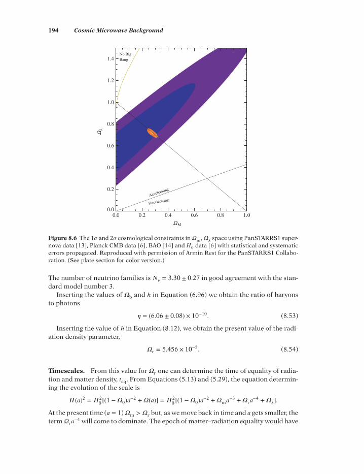
194 Cosmic Microwave Background
0.0 0.2 0.4 0.6 0.8 1.0
ΩM
0.0
0.2
0.4
0.6
0.8
1.0
1.2
1.4
Ωλ
DeceleratingAccelerating
No BigBang
Figure 8.6 The 1𝜎 and 2𝜎 cosmological constraints in𝛺m,𝛺𝜆
space using PanSTARRS1 super-nova data [13], Planck CMB data [6], BAO [14] and H0 data [6] with statistical and systematicerrors propagated. Reproduced with permission of Armin Rest for the PanSTARRS1 Collabo-ration. (See plate section for color version.)
The number of neutrino families is 𝑁𝜈= 3.30 ± 0.27 in good agreement with the stan-
dard model number 3.Inserting the values of 𝛺b and ℎ in Equation (6.96) we obtain the ratio of baryons
to photons
𝜂 = (6.06 ± 0.08) × 10−10. (8.53)
Inserting the value of ℎ in Equation (8.12), we obtain the present value of the radi-ation density parameter,
𝛺r = 5.456 × 10⁻⁵. (8.54)
Timescales. From this value for 𝛺r one can determine the time of equality of radia-tion and matter density, 𝑡eq. From Equations (5.13) and (5.29), the equation determin-ing the evolution of the scale is
𝐻(𝑎)2 = 𝐻20 [(1 −𝛺0)𝑎−2 +𝛺(𝑎)] = 𝐻2
0 [(1 −𝛺0)𝑎−2 +𝛺m𝑎−3 +𝛺r𝑎
−4 +𝛺𝜆].
At the present time (𝑎 = 1)𝛺m > 𝛺r but, as we move back in time and 𝑎 gets smaller, theterm𝛺r𝑎
−4 will come to dominate. The epoch of matter–radiation equality would have

Model Testing and Parameter Estimation 195
occurred when 𝛺m𝑎−3 = 𝛺r𝑎
−4. Using the value of 𝛺m from (8.50) and 𝛺r from (8.54)would give 𝑎−1 = 1 + 𝑧 ≈ 5773. This is not correct, however, because the 𝑎 dependenceof 𝛺r should actually be given by
𝛺r(𝑎) =𝑔∗(𝑎)
2𝑎S𝑇
4
𝜌c=𝑔∗(𝑎)
2𝑎S
𝜌c
(2.725𝑎
)4
, (8.55)
using the function 𝑔∗ discussed in Chapter 5. In the region of 1 + 𝑧 ≳ 1000 neutrinoswill be relativistic and 𝑔∗ = 3.36 instead of 2 [the contribution to the integral in Equa-tion (5.55) from large 𝑧 ≳ 108, where 𝑔∗(𝑎) > 3.36 is negligible]. Temperature scalesinversely with 𝑎, thus at 𝑧eq = 3280 from WMAP 9-year data [12].
Inserting the values of the energy densities in Equations (8.50) and (8.53) intoEquation (5.55), one finds the age of the Universe to a remarkable precision,
𝑡0 = 13.82 ± 0.05 Gyr, (8.56)
is in excellent agreement with the independent determinations of lesser precision inSection 1.5. The WMAP team have also derived the redshift and age of the Universeat last scattering and the thickness of the last scattering shell (noting that the WMAPteam use the term decoupling where we have used last scattering surface—see our def-initions in Section 6.3):
𝑡LSS = 0.379+0.008−0.007 Myr, 𝛥𝑡LSS = 0.118+0.003
−0.002 Myr,
1 + 𝑧LSS = 1089 ± 1, 𝛥𝑧LSS = 195 ± 2.
}(8.57)
Deceleration Parameter. Recalling the definitions
𝐻0 =��0
𝑎0, 𝛺m =
8𝜋𝐺𝜌m
3𝐻20
, 𝛺𝜆= 𝜆
3𝐻20
, 𝑞0 = −��0
𝑎0𝐻20
,
and ignoring 𝛺r, since it is so small, we can find relations between the dynamicalparameters 𝛺
𝜆, 𝛺m, 𝐻0, and the deceleration parameter 𝑞0. Substitution of these
parameters into Equations (5.17) and (5.18) at present time 𝑡0, gives
𝐻20 + 𝑘𝑐
2
𝑎20
− 𝜆
3= 𝛺m𝐻
20 , (8.58)
−2𝑞0𝐻20 +𝐻2
0 + 𝑘𝑐2
𝑎20
− 𝜆 = −3𝛺m𝐻20𝑤, (8.59)
where 𝑤 denotes the equation of state 𝑝m∕𝜌m𝑐2 of matter.
We can then obtain two useful relations by eliminating either 𝑘 or 𝜆. In the firstcase we find
𝛺m(1 + 3𝑤) = 2𝑞0 + 2𝛺𝜆, (8.60)
and, in the second case,
32𝛺m(1 +𝑤) − 𝑞0 − 1 = 𝑘𝑐
2
𝑆20𝐻
20
. (8.61)
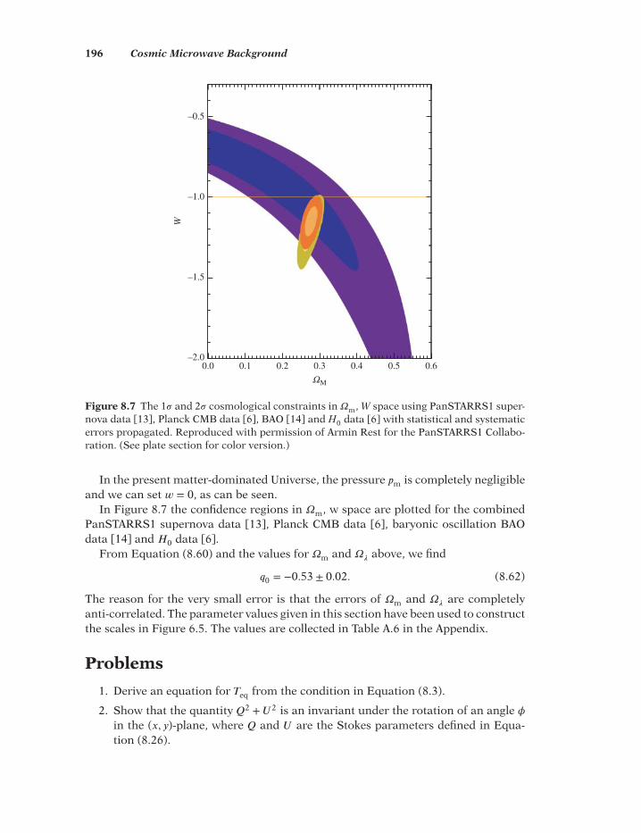
196 Cosmic Microwave Background
0.0 0.1 0.2 0.3 0.4 0.5 0.6
ΩM
–2.0
–1.5
–1.0
–0.5
W
Figure 8.7 The 1𝜎 and 2𝜎 cosmological constraints in𝛺m, W space using PanSTARRS1 super-nova data [13], Planck CMB data [6], BAO [14] and H0 data [6] with statistical and systematicerrors propagated. Reproduced with permission of Armin Rest for the PanSTARRS1 Collabo-ration. (See plate section for color version.)
In the present matter-dominated Universe, the pressure 𝑝m is completely negligibleand we can set 𝑤 = 0, as can be seen.
In Figure 8.7 the confidence regions in 𝛺m, w space are plotted for the combinedPanSTARRS1 supernova data [13], Planck CMB data [6], baryonic oscillation BAOdata [14] and 𝐻0 data [6].
From Equation (8.60) and the values for 𝛺m and 𝛺𝜆
above, we find
𝑞0 = −0.53 ± 0.02. (8.62)
The reason for the very small error is that the errors of 𝛺m and 𝛺𝜆
are completelyanti-correlated. The parameter values given in this section have been used to constructthe scales in Figure 6.5. The values are collected in Table A.6 in the Appendix.
Problems
1. Derive an equation for 𝑇eq from the condition in Equation (8.3).
2. Show that the quantity 𝑄2 + 𝑈2 is an invariant under the rotation of an angle 𝜙in the (𝑥, 𝑦)-plane, where 𝑄 and 𝑈 are the Stokes parameters defined in Equa-tion (8.26).
Model Testing and Parameter Estimation 197
3. Use Wien’s constant, Equation (6.120) and the CMB temperature to determinethe wavelength of the CMB.
4. Use the present radiation-energy density to calculate the pressure due to radia-tion in the Universe.
5. Show that an observer moving with velocity 𝛽 in a direction 𝜃 relative to theCMB sees the rest frame blackbody spectrum with temperature 𝑇 as a blackbodyspectrum with temperature
𝑇′ = 𝑇
𝛾(1 − 𝛽 cos 𝜃). (8.63)
To first order in 𝛽 this gives the dipole anisotropy Equation (8.17) [1].
6. The dipole anisotropy is measured to be 1.2 × 10⁻³𝑇0. Derive the velocity of Earthrelative to the comoving coordinate system.
7. Use Equation (5.55) and 𝛺𝜆= 0.685 to express 𝑡eq in years.
References[1] Peebles, P. J. E., Page, Jr., L. A. et al. Partridge, R. B. 2009 Finding the Big Bangl cosmology.
Cambridge University Press.[2] Mather, J. C., Cheng, E. S., Eplee, R. E. et al. 1990 Astrophys. J. Lett. 354, L37.[3] Fixsen, D. J. et al. 1996 Astrophys. J. 473, 576.[4] Bennett, C. L. et al. 1996 Astrophys. J. Lett. 464, L1.[5] Lynden-Bell, D. et al. 1988 Astrophys. J. 326, 19.[6] Planck Collaboration: Ade, P. A. R. et al. 2014 Astron. Astrophys and preprint
arXiv:1303.5076 [astro-ph.CO].[7] Smoot, G. and Davidson, K. 1993 Wrinkles in time. Avon Books, New York.[8] BICEP2 Collaboration: Ade, P. A. R. et al. 2014 Preprint arXiv:1403.3985 [astro-ph.CO].[9] Kosowsky, A. 1999 New Astronom. Rev. 43, 157.
[10] Kovac, J. et al. 2002 Nature 420, 772.[11] Colless, M. et al. 2001 Mon. Not. R. Astron. Soc. 328, 1039.[12] Bennett, C. L. et al. 2013 Astrophys. J. Suppl. 208, 20 and earlier WMAP papers.[13] Rest, A. et al. 2013 Preprint arXiv:1310.3828 [astro-ph.CO].[14] Blake, C. et al. 2011 Mon. Not. R. Astron. Soc. 418, 1707.[15] Bennett, C. L. et al. 2014, Astrophys. J. 794, 135.


9
Dark Matter
The analysis of anisotropies in the cosmic microwave background have shown thatthe fraction 𝛺c = 0.263 of all the matter in the Universe is nonbaryonic. All formsof radiating baryonic mass are already accounted for in 𝛺b: starlight amounts to𝛺∗ = 0.001–0.002, gas and star remnants in galaxies amount to 𝛺lum < 0.01. The inter-galactic gas contains hydrogen clouds and filaments seen by its Ly𝛼 absorption, warmgas in groups of galaxies radiates soft X-rays, hot gas in clusters is seen in keV X-raysand in the SZE. The missing fraction is not radiating in any wavelength and is there-fore called dark matter.
This term is generic for observed gravitational effects on all scales: galaxies, smalland large galaxy groups, clusters and superclusters, CMB anisotropies over the fullhorizon, baryonic oscillations over large scales, and cosmic shear in the large-scalematter distribution. The correct explanation or nature of dark matter is not known,whether it implies unconventional particles or modifications to gravitational theory.but gravitational effects have convincingly proved its existence in some form.
The remarkable fact is that the dark matter fraction is much larger than the knownfraction and that it does not interact with ordinary baryonic matter except gravita-tionally. The purpose of this Chapter is to summarize the phenomenology of all sucheffects except CMB which was covered in Chapter 8.
In Section 9.1 we study kinematical and dynamical effects: the virial theorem,empirical halo profiles and examples of virially bound groups and clusters. InSection 9.2 we study dark matter in galaxies: spirals, ellipticals, dwarf sphericals,and some arguments on galaxy formation. In Section 9.3 we turn to clusters and inSection 9.4 meet several cases of merging clusters. In Section 9.5 we list possiblecandidates of dark matter. As we shall see, there are no good candidates, only somehypothetical particles which belong to speculative theories.
In Section 9.6 we turn to observations of galaxy distributions and comparisons withsimulations based on the cold dark matter (CDM) paradigm and to predictions andverifications based on the CDM paradigm.
Introduction to Cosmology, Fourth Edition. Matts Roos© 2015 John Wiley & Sons, Ltd. Published 2015 by John Wiley & Sons, Ltd.

200 Dark Matter
9.1 Virially Bound Systems
The planets move around the Sun along their orbits with orbital velocities balancedby the total gravity of the Solar system. Similarly, stars move in galaxies in orbits withorbital velocities 𝑣 determined by the gravitational field of the galaxy, or they movewith velocity dispersion 𝜎. Galaxies in turn move with velocity dispersion 𝜎 underthe influence of the gravitational field of their environment, which may be a galaxygroup, a cluster or a supercluster. Dark matter forms halos which extend far beyondthe luminous matter.
Dynamics. In the simplest dynamical framework one treats massive systems (galax-ies, groups and clusters) as statistically steady, spherical, self-gravitating systems of 𝑁objects with average mass 𝑚 and average velocity 𝑣 or velocity dispersion 𝜎. The totalkinetic energy 𝐸 of such a system is then (we now use 𝜎 rather than 𝑣)
𝐸 = (1∕2)Nm𝜎2. (9.1)
If the average separation is 𝑟, the potential energy of 𝑁(𝑁 − 1)∕2 pairings is
𝑈 = −(1∕2)𝑁(𝑁 − 1)𝐺𝑚2∕𝑟. (9.2)
The virial theorem states that for such a system
𝐸 = −𝑈∕2. (9.3)
The total dynamic mass 𝑀dyn can then be estimated from 𝜎 and 𝑟
𝑀dyn = Nm = 2𝑟𝜎2∕𝐺. (9.4)
This can also be written
𝜎2 ∝ (𝑀dyn∕𝐿)IR, (9.5)
where 𝐼 is a surface luminosity, 𝑅 is a scale, and 𝑀dyn∕𝐿 is the mass to light ratio.Choosing the scale to be the half light radius 𝑅
𝑒, this implies a relationship between
the observed central velocity dispersion 𝜎0, 𝐼𝑒
and 𝑅𝑒
called the Fundamental Plane.of the form
𝑅𝑒∝ (𝜎0)𝑎(𝐼𝑒)𝑏. (9.6)
The virial theorem predicts the values 𝑎 = 2, 𝑏 = 1 for the coefficients. This relationshipis found in ellipticals and in some other types of stellar populations with somewhatdifferent coefficients.
Halo Density Profiles. Dark matter halos in galaxies and clusters can of course notbe observed by their radiation, but there is an excellent tool to determine their sizesand weights: lensing. This we described in full detail in Section 4.3.
The shapes of DM halos in galaxies and clusters need to be simulated or fitted byempirical formulae. Mostly the shape is taken to be spherically symmetric so that thetotal gravitating mass profile 𝑀(𝑟) depends on three parameters: the mass proportion

Virially Bound Systems 201
in stars, the halo mass and the length scale. A frequently used radial density profileparametrization is
𝜌DM(𝑟) = 𝜌0∕[(𝑟∕𝑟s)𝛼(1 + 𝑟∕𝑟s)3−𝛼], (9.7)
where 𝜌0 is a normalization constant and 0 ⩽ 𝛼 ⩽ 3∕2. A standard choice is 𝛼 = 1for the Navarro–Frenk–White profile (NFW) [1] This presents a singularity at 𝑟 → 0although the total integrated mass is finite. The sharp rise of the density at the halocenter forms a “cusp”. Another cusped profile is that of Moore et al. [2] with 𝛼 = 3∕2.
The Einasto profile [3 and earlier references therein] is defined as
𝜌DM(𝑟) = 𝜌𝑒exp{−𝑑
𝑛[(𝑟∕𝑟
𝑒)1∕𝑛 − 1]}, (9.8)
where the term 𝑑𝑛
is a function of 𝑛 such that 𝜌𝑒
is the density at 𝑟𝑒, which defines a
volume containing half of the total mass. At 𝑟 = 0 the density is then finite and theprofile is cored.
The Burkert profile [4] has a constant density core
𝜌DM(𝑟) = 𝜌0∕[(1 + 𝑟∕𝑟𝑠)(1 + (𝑟∕𝑟
𝑠)2)], (9.9)
which appears to fit dwarf galaxy halos well.Some clusters are not well fitted by any spherical approximation. The halo may
exhibit a strong ellipticity or triaxiality in which case none of the above profiles isgood, or the cluster (like Coma) has a binary center.
The dependence of the physical size of clusters on the mass, characterized by themass concentration index 𝑐 ≡ 𝑟vir∕𝑟𝑠, has been studied in 𝛬CDM simulations. At inter-mediate radii 𝑐 is a crucial quantity in determining the density profile.
The Local Group. The Local Group (LG) is a very small virial system, dominatedby two large galaxies, the M31 or Andromeda galaxy, and the Milky Way. The M31exhibits blueshift, falling in towards us. Evidently our Galaxy and M31 form a boundsystem together with all or most of the minor galaxies in the Local Group. The LocalGroup extends to about 3 Mpc and the velocity dispersions of its members is about200 km s−1. The virial mass is 𝑀vir = 8.2+2.5
−1.6 𝑀⊙
.In this group the two large galaxies dominate the dynamics, so that it is not mean-
ingful to define a statistically average pairwise separation between galaxies, nor anaverage mass nor an average orbital velocity. The total kinetic energy 𝐸 is still givenby the sum of all the group members, and the potential energy 𝑈 by the sum of all thegalaxy pairs, but here the pair formed by the M31 and the Milky Way dominates, andthe pairings of the smaller members with each other are negligible.
Observations of galaxies in the LG can be used to constrain the nature of DM. Thenumber of low mass satellites of MW and M31 as compared with CDM predictions canbe explained through the effects of gas-dynamics on baryons, making them invisible,or they can simply not exist, if DM particles have a mass in the keV scale.
Small Galaxy Groups. There are other examples of groups formed by a small num-ber of galaxies which are enveloped in a large cloud of hot gas, visible by its X-ray

202 Dark Matter
emission. One may assume that the electron density distribution associated with theX-ray brightness is in hydrostatic equilibrium, and one can extract the ICM radialdensity profiles by fits.
The amount of matter in the form of hot gas can be deduced from the intensity ofthis radiation. Adding the gas mass to the observed luminous matter, the total amountof baryonic matter, 𝑀b, can be estimated. In clusters studied, the gas fraction increaseswith the distance from the center; the dark matter appears more concentrated thanthe visible matter.
The temperature of the gas depends on the strength of the gravitational field, fromwhich the total amount of gravitating matter, 𝑀grav, in the system can be deduced.In many such small galaxy groups one finds 𝑀grav∕𝑀b ⩾ 3, testifying to a dark halopresent. An accurate estimate of 𝑀grav requires that also dark energy is taken intoaccount, because it reduces the strength of the gravitational potential. There are some-times doubts whether all galaxies appearing near these groups are physical members.If not, they will artificially increase the velocity scatter and thus lead to larger virialmasses.
On the scale of large clusters of galaxies like the Coma, it is generally observed thatDM represents about 85% of the total mass and that the visible matter is mostly in theform of a hot ICM.
The Local Universe. The Local Universe is the best observed part of the universe inwhich least massive and faintest objects can be detected and studied in detail. Theseobservations resulted in a new research field called Near-Field Cosmology, and havemotivated cosmologists to study the Local Group archaeology in their quest for under-standing galaxy formation and the play dark matter has on it.
In a volume of a diameter of 96 Mpc beyond the local group Karachentsev [6] hasstudied 11,000 galaxies appearing single, in pairs, in triplets and in groups. Most ofthem belong to the Local Supercluster (LSC) and they constitute < 15% of the mass ofthe Virgo Supercluster. The radial velocities are 𝑣 < 3500 km s−1. These galaxies canbe treated as a virial system with average density 𝛺m,local = 0.08 ± 0.02, surprisinglysmall compared to the global density parameter. The fact that much more low massDM halos are predicted by cosmological simulations than low luminosity galaxies areobserved can be explained by gas-dynamical processes which prevent star formationin low mass halos.
Karachentsev quotes [6] three proposed explanations for this mass deficit.
• Dark matter in the systems of galaxies extends far beyond their virial radius, sothat the total mass of a group or cluster is three to four times larger than thevirial estimate. However, this contradicts other existing data.
• The diameter of the considered region of the Local universe, 90 Mpc, does notcorrespond to the true scale of the “homogeneity cell”; our Galaxy may be locatedinside a giant void sized about 100–500 Mpc, where the mean density of matteris three to four times lower than the global value. However, the location of ourGalaxy is characterized by an excess, rather than by a deficiency of local densityat all scales up to 45 Mpc.

Galaxies 203
• Most of the dark matter in the Universe, or about two thirds of it, is not associ-ated with groups and clusters of galaxies, but distributed in the space betweenthem in the form of massive dark clumps or as a smooth “ocean”. It is as yetdifficult to evaluate this proposal.
Clearly the physics in the Local Universe does not prove the existence of dark mat-ter, rather it brings in new problems.
9.2 GalaxiesSpiral Galaxies. The spiral galaxies are stable gravitationally bound systems inwhich matter is composed of stars and interstellar gas. Most of the observable mat-ter is in a relatively thin disc, where stars and gas travel around the galactic centeron nearly circular orbits. Visible starlight traces velocity out to radial distances typi-cally of the order of 10 kpc, and interstellar gas out to 20–50 kpc. The luminous partsof galaxies, as evidenced by radiation of baryonic matter in the visible, infrared andX-ray spectra, account only for 𝛺lum < 0.01.
By observing the Doppler shift of the integrated starlight and the radiation at𝜆 = 0.21 m from the interstellar hydrogen gas, one finds that spiral galaxies rotate.If the circular velocity at radius 𝑟 is 𝑣 in a galaxy of mass 𝑀 , the condition for stabilityis that the centrifugal acceleration should equal the gravitational pull:
𝑣2
𝑟= GM
𝑟2. (9.10)
In other words, the radial dependence of the velocity of matter rotating in a disc isexpected to follow Kepler’s law 𝑣 =
√GM∕𝑟.
The surprising result for spiral galaxy rotation curves is, that the velocity does notfollow Kepler’s inverse-root law, but stays rather constant after attaining a maximumat about 5 kpc. The most obvious solution to this is that the galaxies are embedded inextensive, diffuse halos of dark matter. In fact, to explain the observations that 𝑣(𝑟) ≈constant the radial mass distribution 𝑀(𝑟) must be proportional to 𝑟 and the radialdensity profile is
𝜌(𝑟) ∝ 𝑟−2. (9.11)
Assuming that the disc-surface brightness is proportional to the surface density ofluminous matter, one derives a circular speed which is typically more than a factor ofthree lower than the speed of the outermost measured points [5]. This implies that thecalculated gravitational field is too small by a factor of 10 to account for the observedrotation.
There are only a few possible solutions to this problem. One is that the theoryof gravitation is wrong. It is possible to modify ad hoc Kepler’s inverse square law orNewton’s assumption that 𝐺 is a constant, but the corresponding modifications cannotbe carried out in the relativistic theory, and a general correlation between mass andlight remains. The modifications would have to be strong at large scales, and thiswould greatly enhance cosmic shear, which is inconsistent with measurements.
Another possibility is that spiral galaxies have magnetic fields extending out toregions of tens of kiloparsecs where the interstellar gas density is low and the gas

204 Dark Matter
dynamics may easily be modified by such fields [6]. But this argument works only onthe gas halo, and does not affect the velocity distribution of stars. Also, the existenceof magnetic fields of sufficient strength remains to be demonstrated; in our Galaxy itis only a few microgauss, which is insufficient.
The accepted solution is then that there exist vast amounts of nonluminous DMbeyond that accounted for by luminous, baryonic matter. One natural place to look forDM is in the neighborhood of the Solar System. In 1922, Jacobus C. Kapteyn deducedthat the total density in the local neighborhood is about twice as large as the luminousdensity in visible stars. Although the result is somewhat dependent on how large onechooses this ‘neighborhood’ to be, modern dynamical estimates are similar.
Our Galaxy is complicated because of what appears to be a noticeable density dipat 9 kpc and a smaller dip at 3 kpc. To fit the measured rotation curve one needs atleast three contributing components: a central bulge, the star disk + gas, and a DMhalo. No DM component appears to be needed until radii beyond 15 kpc.
The rotation curve of most galaxies can be fitted by the superposition of contri-butions from the stellar and gaseous disks, sometimes a bulge, and the dark halo,modeled by a quasi–isothermal sphere. The inner part is difficult to model becausethe density of stars is high, rendering observations of individual star velocities diffi-cult. Thus the fits are not unique, the relative contributions of disk and dark matterhalo is model-dependent, and it is sometimes not even sure whether galactic disks docontain dark matter. Typically, dark matter constitutes about half of the total mass.
In Figure 9.1 we show the rotation curves fitted for 11 well-measured galaxies [7]of increasing halo mass. One notes, that the central dark halo component is indeedmuch smaller than the luminous disk component. At large radii, however, the need fora DM halo is obvious. On galactic scales, the contribution of DM generally dominatesthe total mass. Note the contribution of the baryonic component, negligible for lightmasses but increasingly important in the larger structures.
It appears that cusped profiles are in clear conflict with data on spiral galaxies.Central densities are rather flat, scaling approximately as 𝜌0 ∝ 𝑟
−2∕3luminous
. The best-fitdisk + NFW halo mass model fits the rotation curves poorly, it implies an implausiblylow stellar mass to light ratio and an unphysically high halo mass. Clearly the actualprofiles are of very uncertain origin.
One notes in Figure 9.1 that the shape of the rotation curve depends on the halovirial mass so that the distribution of gravitating matter is luminosity dependent. Theold idea that the rotation curve stays constant after attaining a maximum is thus a sim-plification of the real situation. The rotation velocity can be expressed by a UniversalRotation Curve [7]: all spiral galaxies appear to lie on a curve in the four-dimensionalspace of luminosity, core radius, halo central density and fraction of DM.
What is required to explain the Universal Rotation Curve and the cored profiles issome kind of interaction between baryons and dark matter, which has not met withany success. A more successful idea may be dark matter self-interaction.
Elliptical Galaxies. Elliptical galaxies are quite compact objects which mostly lackneutral gas and which do not rotate so their mass cannot be derived from rotationcurves. The total dynamical mass is then the virial mass as derived from the velocity

Galaxies 205
<MI> = –18.5
<MI> = –20.5
.5
0V
(R)/
V(R
apt)
V(R
)/V
(Rap
t)V
(R)/
V(R
apt)
V(R
)/V
(Rap
t)0 .5 1 1.5 2
1
.5
00 .5 1 1.5 2
1
.5
00 .5 1 1.5 2
1
.5
00 .5 1 1.5 2
1
.5
00 .5 1 1.5 2
1
.5
00 .5 1 1.5 2
1
.5
00 .5 1 1.5 2
1
.5
00 .5 1 1.5 2
1
.5
00 .5 1 1.5 2
1
.5
00 .5 1 1.5 2
1
.5
00 .5 1 1.5 2
1
<MI> = –19.4
<MI> = –20.9 <MI> = –21.2
<MI> = –21.6 <MI> = –22.0 <MI> = –22.2
<MI> = –22.6 <MI> = –23.2 R/Rapt
R/Rapt R/Rapt
<MI> = –20.0
Figure 9.1 The rotation curves fitted for 11 well-measured galaxies of increasing halo mass[7].
dispersions of stars and the anisotropies of their orbits. However, to disentangle thetotal mass profile into its dark and its stellar components is not straightforward,because the dynamical mass decomposition of dispersions is not unique. The lumi-nous matter in the form of visible stars is a crucial quantity, indispensable to infer thedark component. When available one also makes use of strong and weak lensing data,and of the X-ray properties of the emitting hot gas. The gravity is then balanced bypressure gradients as given by Jeans’ Equation (see Chapter 11).
Inside the half light radius 𝑅𝑒
the contribution of the dark matter halo to the cen-tral velocity dispersion is often very small, it is dominated by the stars, so that thedark matter profile is intrinsically unresolvable. On the average the dark matter com-ponent contributes less than 5% to the total velocity dispersions. The outer mass pro-file is compatible with the NFW Equation (9.7) and Burkert Equation (9.9) formuli.Important information on the mass distribution can be obtained from the Fundamen-tal Plane, Equation (9.6). which yields the coefficients 𝑎 = 1.8, 𝑏 = 0.8. Note that this

206 Dark Matter
is in some tension with the Virial Theorem, perhaps due to variations in the centraldispersions, 𝜎0, of the stellar populations.
Most of the baryons in optically selected, isolated, elliptical galaxies are in a mor-phologically relaxed hot gas halo detectable out to ≈ 200 kpc, that is well describedby hydrostatic models. The isolation condition reduces the influence of a possiblegroup-scale or cluster-scale halo. The baryons and the dark matter conspire to pro-duce a total mass density profile that can be well-approximated by a power law,𝜌tot ∝ 𝑟−𝛼 over a wide range.
The fitting method involves solving the equation of hydrostatic equilibrium to com-pute temperature and density profile models, given parametrized mass and entropyprofiles. The models are then projected onto the sky and fitted to the projected tem-perature and density profiles. Fits fit ignoring DM are poor, but the inclusion of DMmay improve the fits highly significantly; in one study DM was required at 8.2𝜎. In sev-eral studies, for most of the radii, the dark matter contribution is very small althoughstatistically significant.
Dwarf Spheroidal Galaxies. The mass to light ratio of an astronomical object isdefined as 𝛶 ≡ 𝑀∕𝐿. Dwarf spheroidal galaxies (dSph) are the smallest stellar sys-tems containing dark matter and exhibit very high 𝛶 = 𝑀∕𝐿 ratios, 𝛶 = 10–100. InAndromeda IX 𝛶 =93+ 120/–50, in Draco 𝛶 = 330 ± 125. The dwarf spheroidals haveradii of ≈ 100 pc and central velocity dispersions ≈ 10 km s−1 which is larger thanexpected for self-gravitating, equilibrium stellar populations. The generally acceptedpicture has been, that dwarf galaxies have slowly rising rotation curves and are dom-inated by dark matter at all radii.
However, Swaters et al. [8] have reported observations of H I rotation curves for asample of 73 dwarf galaxies, among which eight galaxies have sufficiently extendedrotation curves to permit reliable determination of the core radius and the centraldensity. They found that dark matter only becomes important at radii larger thanthree or four disk scale lengths. Their conclusion is, that the stellar disk can explainthe mass distribution over the optical parts of the galaxy. Some of the required stellarmass to light ratios are high, up to 15 in the R-band.
Comparing the properties of dwarf galaxies in both the core and outskirts of thePerseus Cluster, Penny and Conselice [9] found a clear correlation between mass tolight ratio and the luminosity of the dwarfs, such that the faintest dwarfs require thelargest fractions of dark matter to remain bound. This is to be expected, as the faintera galaxy is, the less luminous mass it will contain, therefore the higher its dark mattercontent must be to prevent its disruption. Dwarfs are more easily influenced by theirenvironment than more massive galaxies.
The distance to the Perseus Cluster prevents an easy determination of 𝛶 , so Pennyand Conselice [9] instead determined the dark matter content of the dwarfs by cal-culating the minimum mass needed in order to prevent tidal disruption by the clus-ter potential, using their sizes, the projected distance from the cluster center to eachdwarf and the mass of the cluster interior. Three of 15 dwarfs turned out to have massto light ratios smaller than 3, indicating that they do not require dark matter.

Galaxies 207
Ultra-compact dwarf galaxies (UCDs) are stellar systems with masses of around107–108 Msun and half-mass radii of 10–100 pc. A remarkable properties of UCDs isthat their dynamical mass to light ratios are on average about twice as large as thoseof globular clusters of comparable metallicity, and also tend to be larger than whatone would expect based on simple stellar evolution models. UCDs appear to containvery little or no dark matter.
Collisional N-body simulations of the coevolution of a system composed of starsand dark matter find that DM gets removed from the central regions of such systemsdue to dynamical friction and mass segregation of stars. The friction timescale is sig-nificantly shorter than a Hubble time for typical globular clusters, while most UCDshave friction times much longer than a Hubble time. Therefore, a significant darkmatter fraction may remain within the half-mass radius of present-day UCDs, mak-ing dark matter a viable explanation for their elevated mass to light ratios.
A different type of systems are the ultra-faint dwarf galaxies (UFDs). When inter-preted as steady state objects in virial equilibrium they would be the most DM domi-nated objects known in the Universe. Their half-light radii range from 70 to 320 pc.
A special case is the UFD disk galaxy Segue 1 [10] which has a baryon mass ofonly about 1000 solar masses. One interpretation is that this is a thin non-rotatingstellar disk not accompanied by a gas disk, embedded in an axisymmetric DM haloand with a ratio 𝑓 ≡ 𝑀halo∕𝑀b ≈ 200. But if the disk rotates, 𝑓 could be as high as2000. If Segue 1 also has a magnetized gas disk, the dark matter halo has to confinethe effective pressure in the stellar disk and the magnetic Lorentz force in the gas diskas well as possible rotation. Then 𝑓 could be very large [10]. Another interpretation isthat Segue 1 is an extended globular cluster rather than an UFD.
Primordial Density Fluctuations. Galaxies form by gas cooling and condensinginto DM haloes, where they turn into stars. The star-formation rate is 10𝑀
⊙yr−1 in
galaxies at 2.8 < 𝑧 < 3.5 for which the Ly𝛼 break at 91.2 nm shifts significantly (at 𝑧 = 3it has shifted to 364.8 nm). Galaxy mergers and feedback processes also play majorroles.
Galaxy formation requires the study of how galaxies populate DM halos. In sim-ulations one attempts to track galaxy and DM halo evolution across cosmic time ina physically consistent way, providing positions, velocities, star formation histories,abundance matching arguments and other physical properties for the galaxy popula-tions of interest.
The implied spatial clustering of stellar mass turns out to be in remarkably goodagreement with a direct and precise measurement. By comparing the galaxy massautocorrelation function with the mass autocorrelation function averaged over theLocal Supercluster (LSC) volume, one concludes that a large amount of matter in theLSC is dark.
Over a wide range of scales there appears to be a universal relation between densityand size of observed dark matter halos, from dwarf galaxies to galaxy clusters. Sucha universal property is difficult to explain without dark matter.
208 Dark Matter
The very general question arises whether the galaxies could at all have formedfrom primordial density fluctuations in a purely baryonic medium. As we have noted,the fluctuations in radiation and matter maintain adiabaticity. The amplitude of theprimordial baryon density fluctuations would have needed to be very large in orderto form the observed number of galaxies. But then the amplitude of the CMB fluctua-tions would also have been very large, leading to intolerably large CMB anisotropiestoday. Thus galaxy formation in purely baryonic matter is ruled out by this argumentalone. The galaxies could only have formed in the presence of gravitating dark matterwhich started to fluctuate early, unhindered by radiation pressure.
9.3 ClustersThe Coma Cluster. Historically, the first observation of dark matter in an object at acosmological distance was made by Fritz Zwicky in 1933 [5]. While measuring radialvelocity dispersions of member galaxies in the Coma cluster (that contains some 1000galaxies), and the cluster radius from the volume they occupy, Zwicky was the first touse the virial theorem to infer the existence of unseen matter. He found to his surprisethat the dispersions were almost a factor of ten larger than expected from the summedmass of all visually observed galaxies in the Coma. He concluded that in order tohold galaxies together the cluster must contain huge amounts of some nonluminousmatter. From the dispersions he concluded that the average mass of galaxies withinthe cluster was about 160 times greater than expected from their luminosity (a valuerevised today), and he proposed that most of the missing matter was dark.
Zwicky’s suggestion was not taken seriously at first by the astronomical communitywhich Zwicky felt as hostile and prejudicial. Clearly, there was no candidate for thedark matter because gas radiating X-rays and dust radiating in the infrared could notyet be observed, and nonbaryonic matter was unthinkable–even the neutron had notbeen discovered yet. Only some 40 years later when studies of motions of stars withingalaxies also implied the presence of a large halo of unseen matter extending beyondthe visible stars, dark matter became a serious possibility.
Since that time, modern observations have revised our understanding of the com-position of clusters. Luminous stars represent a very small fraction of a cluster mass;in addition there is a baryonic, hot intracluster medium (ICM) visible in the X-ray spec-trum. Rich clusters typically have more mass in hot gas than in stars; in the largestvirial systems like the Coma the composition is about 85% DM, 14% ICM and only1% stars.
In modern applications of the virial theorem one also needs to model andparametrize the radial distributions of the ICM and the dark matter densities. In theoutskirts of galaxy clusters the virial radius roughly separates bound galaxies fromgalaxies which may either be infalling or unbound. The virial radius 𝑟vir is convention-ally defined as the radius within which the mean density is 200 times the backgrounddensity.
Matter accretion is in general quite well described within the approximation of theSpherical Collapse Model. According to this model, the velocity of the infall motion

Clusters 209
and the matter overdensity are related. Mass profile estimation is thus possible oncethe infall pattern of galaxies is known.
Dark matter is usually dissected from baryons in lensing analyses by first fitting thelensing features to obtain a map of the total matter distribution and then subtractingthe gas mass fraction as inferred from X-ray observations. The total mass map canthen be obtained with parametric models in which the contribution from cluster-sizedDM halos is considered together with the main galactic DM halos. Mass in stars and instellar remnants is estimated converting galaxy luminosity to mass assuming suitablestellar mass to light ratios.
One may go one step further by exploiting a parametric model which has threekinds of components: cluster-sized DM halos, galaxy-sized (dark plus stellar) matterhalos, and a cluster-sized gas distribution. In systems of merging clusters DM maybecome spatially segregated from baryonic matter and thus observable. We shall meetseveral such cases later in this Chapter.
The Local Supercluster (LSC). The autocorrelation function 𝜉(𝑟) in Equation (9.8)was defined for distances 𝑟 in real space. In practice, distances to galaxies are mea-sured in redshifts, and then two important distortions enter. To describe the sepa-ration of galaxy pairs on the surface of the sky, let us introduce the coordinate 𝜎,transversal to the line of sight, and 𝜋 radial. In redshift space the correlation functionis then described by 𝜉(𝜎, 𝜋) or its spherical average 𝜉(𝑠), where 𝑠 =
√𝜋2 + 𝜎2.
The transversal distance 𝜎 is always accurate, but the radial redshift distance 𝜋
is affected by velocities other than the isotropic Hubble flow. For relatively nearbygalaxies, 𝑟 ⩽ 2 Mpc, the random peculiar velocities make an unknown contribution to𝜋 so that 𝜉(𝑠) is radially distorted. The undistorted correlation function 𝜉(𝑟) is seenisotropic in (𝜎, 𝜋)-space in the top left panel of Figure 9.2. The lower left panel ofFigure 9.2 shows the distortion to 𝜉(𝑠) as an elongation in the 𝜋 direction.
Over large distances where the peculiar velocities are unimportant relative to theHubble flow (tens of Mpc), the galaxies in the LSC feel its attraction, as is manifestedby their infall toward its center with velocities in the range 150–450 km s−1. From thisone can derive the local gravitational field and the mass excess 𝛿𝑀 concentrated in theLSC. The infall velocities cause another distortion to 𝜉(𝑠): a flattening as is shown inthe top right panel of Figure 9.2. When both distortions are included, the correlationfunction in (𝜎, 𝜋)-space looks like the bottom right panel of Figure 9.2. The narrowpeaks in the 𝜋 direction have been seen for a long time, and are called Fingers of God.
If galaxy formation is a local process, then on large scales galaxies must trace mass(on small scales galaxies are less clustered than mass), so that 𝜉gal(𝑟) and 𝜉mass(𝑟) areproportional:
𝜉gal(𝑟) = 𝑏2𝜉mass(𝑟).
Here 𝑏 is the linear bias: bias is when galaxies are more clustered than mass, andanti-bias is the opposite case; 𝑏 = 1 corresponds to the unbiased case. The presenceof bias is an inevitable consequence of the nonlinear nature of galaxy formation. Thedistortions in 𝜉(𝑠) clearly depend on the mass density 𝛺m within the observed volume.

210 Dark Matter
20
10
0
–10
–20
–20
–20 –10 0 10 20 –20 –10 0 10 20
–10
20
10
0
π/h–
1 Mpc
σ/h–1 Mpc σ/h–1 Mpc
π/h–
1 Mpc
Figure 9.2 Plot of theoretically calculated correlation functions 𝜉(𝜎, 𝜋) as described in refer-ence [2]. The lines represent contours of constant 𝜉(𝜎, 𝜋) = 4.0,2.0,0.5,0.2,0.1. The models are:top left, undistorted; bottom left, no infall velocities but 𝛽 = 0.4; top right, infall velocity disper-sion 𝑎 = 500 km s−1, 𝛽 = 0; bottom right, 𝑎 = 500 km s−1, 𝛽 = 0.4. All models use Equation (9.15)with 𝑟c = 5.0ℎ−1 Mpc and 𝛾 = 1.7. Reproduced from [11] by permission of the 2dFGRS Team.
Introducing the phenomenological flattening parameter
𝛽 = 𝛺0.6m ∕𝑏, (9.12)
one can write a linear approximation to the distortion as
𝜉(𝑠)𝜉(𝑟)
= 1 + 2𝛽3
+ 𝛽2
5. (9.13)
Estimates of 𝛽 and 𝑏 which we shall discuss in Equations (9.18–19) lead to a value of𝛺m of the order of 0.25. Thus a large amount of matter in the LSC is dark.

Merging Galaxy Clusters 211
9.4 Merging Galaxy Clusters
In isolated galaxies and galaxy clusters all matter components contributing to thecommon gravitational potential are more or less centrally-symmetrically coincident.This makes it difficult to discern DM from the baryonic components, and dependenton parametrization, as we have discussed in the section on Dynamics. In merginggalaxy clusters however, the separate distributions of galaxies, intracluster gas andDM may become spatially segregated permitting separate observations. The visuallyobservable galaxies behave as collisionless particles, the baryonic intracluster plasmais fluid-like, it experiences ram pressure and emits X-rays, but noninteracting DMdoes not feel that pressure, it only makes itself felt by its contribution to the commongravitational potential.
Major cluster mergers are the most energetic events in the Universe since the BigBang. Shock fronts in the intracluster gas are the key observational tools in the studyof these systems. When a subcluster traverses a larger cluster it cannot be treated as asolid body with constant mass moving at constant velocity. During its passage throughthe gravitational potential of the main cluster it is shrinking over time, stripped of gasenvelope and decelerating. Depending on the ratio of the cluster masses, the gas formsa bow shock in front of the main cluster, and this can even be reversed at the time whenthe potentials coincide.
In several examples of galaxy cluster mergers the presence of DM could be inferredfrom the separation of the gravitational potential from the position of the radiatingplasma.
The Bullet Cluster 1E0657-558. The exceptionally hot and X-ray luminous galaxycluster 1E0657-558, the Bullet cluster at redshift 𝑧 = 0.296, was discovered by Tuckeret al. in 1995 [13] in Chandra X-ray data. Its structure as a merger of a 2.3 ×10¹⁴ 𝑀
⊙
subcluster with a main 2.8 ×10¹⁴𝑀
⊙cluster was demonstrated as the first clear exam-
ple of a bow shock in a heated intracluster plasma. With the advent of high-resolutionlensing, a technique could be developed combining multiple strongly-lensed HubbleSpace Telescope multi-color images of identified galaxies with weakly lensed and ellip-tically distorted background sources. The reconstructed gravitational potential doesnot trace the X-ray plasma distribution which is the dominant baryonic mass com-ponent, but rather approximately traces the distribution of bright cluster membergalaxies.
In early pictures, often reproduced, the center of the total mass was offset fromthe center of the baryonic mass peaks, proving that the majority of the matter in thesystem is unseen. In front of the bullet cluster which has traversed the larger oneabout 100 Myr ago with a relative velocity of 4500 km s−1, a bow shock is evident inthe X-rays. The main cluster peak and the distinct subcluster mass concentration areboth clearly offset from the location of the X-ray gas. We do not reproduce that wellknown figure here because recent analysis of this system [14] do not confirm theseresults, rather they find that dark matter forms three distinct clumps.

212 Dark Matter
The Baby Bullet. Another merging system with similar characteristics but withlower spatial resolution is the post-merging galaxy cluster pair MACS J0025.4-1222,also called the Baby Bullet. It has an apparently simple geometry, consisting of twolarge subclusters of similar richness, about 2.5 × 10¹⁴
𝑀⊙
, both at redshift 𝑧 = 0.586,colliding in approximately the plane of the sky. Multiple images due to strong lensingof four distinct components could be identified.
The two distinct mass peaks are clearly offset by 4𝜎 from the main baryonic com-ponent, which is the radiating hot gas observed by Chandra. The relative mergingvelocity is estimated to be 2000 km s−1. The majority of the mass is spatially coinci-dent with the identified galaxies, which implies that the cluster must be dominatedby a relatively collisionless form of dark matter.
Many clusters exhibit very complicated geometries observed by Chandra. However,in many cases the separation of hot gas from collisionless DM still requires betterlensing data.
“El Gordo.” The Atacama Cosmology Telescope has presented properties for anexceptionally massive merging cluster, the ACT-CL J0102-4915 nicknamed El Gordo atredshift 𝑧 = 0.87 [15]. It was discovered by selection for its bright Sunyaev-Zel’dovich(SZ) effect (described in Section 10.2), confirmed optically and through its ChandraX-ray data. It is the most significant SZ cluster detection to date by nearly a factor oftwo, with an SZ decrement comparable to the Bullet cluster.
The galaxy distribution is double peaked, whereas the peak in the X-ray emissionlies between the density peaks. The X-ray peak forms a relatively cool bullet of lowentropy gas like in the Bullet cluster. In the absence of a weak lensing mass reconstruc-tion, the galaxy distribution can only be used as a proxy for the total mass distribution.Thus to conclude that an offset between baryonic and DM has been demonstrated isyet premature.
Other Mergers. Data acquired with the Advanced Camera for Surveys on the HubbleSpace Telescope, HST, shows that the cluster Abell 2744 [16] is a complicated mergerbetween three or four separate bodies. The position and mass distribution of partof the cluster have been tightly constrained by the strong lensing of 11 backgroundgalaxies producing 31 multiple images. But two clumps lack such images from stronglensing, indicating that they are less massive.
The joint gravitational lensing analysis combines all the strongly lensed multiply-imaged systems and their redshifts with weak lensing shear catalogues to reconstructthe cluster’s lensing potential. The location of shock fronts and velocities, densities andtemperatures in the intracluster medium, and all existing X-ray data from Chandrahave been combined. The lensing mass reconstruction and the luminosity contoursof the emission then shows an extremely complex picture of separations between thedark matter and baryonic components. However, it is difficult to ascertain whetherthis is a single, separate DM structure and to derive decisive separation between DM,X-ray luminous gas and bright cluster member galaxies. One possible interpretationis a near simultaneous double merger 0.12–0.15 Gyr ago.

Dark Matter Candidates 213
Another major cluster merger is DLSCL J0916.2+2951 [17] at 𝑧 = 0.53, in which thecollisional cluster gas has become clearly dissociated from the collisionless galaxiesand dark matter. The cluster was identified using optical and weak-lensing observa-tions as part of the Deep Lens Survey. Follow-up observations with Keck, Subaru,Hubble Space Telescopes, and Chandra show that the cluster is a dissociative mergerwhich constrains the DM self-interaction cross-section to 𝜎𝑚
−1DM ⩽ 7 cm2/g. The system
is observed at least 0.7 ± 0.2 Gyr since first pass-through, thus providing a picture ofcluster mergers 2–5 times further progressed than similar systems observed to date.
9.5 Dark Matter Candidates
If only a small percentage of the total mass of the Universe is accounted for by starsand hydrogen clouds, could baryonic matter in other forms make up DM? The answergiven by nucleosynthesis is a qualified no: all baryonic DM is already included in 𝛺b.
Dark Baryonic Matter. Before the value of 𝛺dm was pinned down as certainly as itis now, several forms of dark baryonic matter was considered. Gas or dust clouds werethe first thing that came to mind. We have already accounted for hot gas because it isradiating and therefore visible. Clouds of cold gas would be dark but they would notstay cold forever. Unless there exists vastly more cold gas than hot gas, which seemsunreasonable, this DM candidate is insufficient.
It is known that starlight is sometimes obscured by dust, which in itself is invis-ible if it is cold and does not radiate. However, dust grains re-radiate starlight inthe infrared, so they do leave a trace of their existence. But the amount of dust androcks needed as DM would be so vast that it would have affected the compositionof the stars. For instance, it would have prevented the formation of low-metallicity(population-II) stars. Thus dust is not an acceptable candidate. And baryons are justtoo few to explain DM.
Snowballs of frozen hydrogenic matter, typical of comets, have also been consid-ered, but they would sublimate with time and become gas clouds. A similar fateexcludes collapsed stars: they eject gas which would be detectable if their numberdensity were sufficient for DM.
A more serious candidate for baryonic matter has been jupiters or brown dwarfs:stars of mass less than 0.08𝑀
⊙. They also go under the acronym MACHO for Mas-
sive Compact Halo Object. They lack sufficient pressure to start hydrogen burning,so their only source of luminous energy is the gravitational energy lost during slowcontraction. Such stars would clearly be very difficult to see since they do not radi-ate. However, if a MACHO passes exactly in front of a distant star, the MACHO wouldact as a gravitational microlens, because light from the star bends around the massiveobject. The intensity of starlight would then be momentarily amplified (on a timescaleof weeks or a few months) by microlensing, as described in Section 4.3. The problemis that even if MACHOs were relatively common, one has to monitor millions of starsfor one positive piece of evidence. Only a few microlensing MACHOs have been dis-covered in the space between Earth and the Large Magellanic Cloud, but not enoughto explain DM.

214 Dark Matter
The shocking conclusion is that the predominant form of matter in the Universeis nonbaryonic, and we do not even know what it is composed of! Thus we are our-selves made of some minor pollutant, a discovery which may well be called the fourthbreakdown of the anthropocentric view. The first three were already accounted for inChapter 1.
Black Holes. Primordial black holes could be good candidates because they evadethe nucleosynthesis bound, they are not luminous, they (almost) do not radiate, and ifthey are big enough they have a long lifetime, as we saw in Equation (5.82). They arebelieved to sit at the center of every galaxy and have masses exceeding 100𝑀
⊙. The
mass range 0.3–30𝑀⊙
is excluded by the nonobservation of MACHOs in the galactichalo (cf. Section 5.4). Various astrophysical considerations limit their mass to around104𝑀
⊙. But black holes cannot be the solution to the galactic rotation curves nor to
merging clusters.
Exotica. At higher scales extra dimensions could exist. the usual(3+1) spacetimecould be a brane embedded in a higher dimensional bulk. Standard model fields wouldbe confined on the brane while gravity propagates in the extra dimension. In this kindof models the hierarchy problem is solved in various ways for example the higherdimensions are compactified on different topologies of scale 𝑅 with the effect of low-ering the Planck scale energy closer to the electroweak scale. Compactification of extradimensions gives rise to a quantization of momentum, 𝑝2 ≃ 1∕𝑅2 of the fields prop-agating in the bulk, and the apparition of a set of Fourier expanded modes [KaluzaKlein (KK) states], for each bulk field. Particles moving in extra dimensions appearas heavy particles with masses 𝑚
𝑛∕𝑅. The new states have the same quantum num-
bers (e.g., charge, color, etc). Another way to reach the same goal is to introduce extradimensions with large curvature.
If extra dimensions are compactified around a circle or torus, the extra-dimensionalmomentum conservation implies conservation of the KK number 𝑛, and the lightestfirst level KK state is stable. Theories with compact extra dimensions can be writtenas theories in ordinary four dimensions by performing a KK reduction.
Among further exotica are solitons, which are nontopological scalar-field quantawith conserved global charge 𝑄 (Q-balls) or baryonic charge 𝐵 (B-balls).
Mirror Matter [18] implies reintroducing. all the known fields with the same cou-pling constants, but with opposite parities. The most natural way to do so is toadd to the existing Lagrangian its parity-symmetric counterpart, so that the wholeLagrangian is invariant under the parity transformation, each part transforminginto the other. We then end up with a new sector of particles, called mirror sector,which is an exact duplicate of the ordinary sector, but where ordinary particles haveleft-handed interactions, mirror particles have right-handed interactions.
As a consequence, the three gauge interactions act separately in each sector, theonly link between them being gravity. Because mirror baryons, just like their ordi-nary counterparts, are stable and can be felt only through their gravitational effects,the mirror matter scenario provides an ideal interpretation of dark matter. Its partic-ularity is that it is a self-interacting candidate, but without any new parameter at the
Dark Matter Candidates 215
level of particle physics. At the cosmological level there are two new parameters, theratio 𝑥 of the temperatures of the ordinary and mirror cosmic background radiations,and the relative amount 𝛽 of mirror baryons compared to the ordinary ones. In thepresence of mirror matter, the matter energy density parameter is
𝛺m = 𝛺b(1 + 𝛽). (9.14)
Scalar fields Suppose that the dark matter particles are described by a spin-0 scalarfield like the QCD axion. A variety of unification theories have proposed other scalarfield candidates, the bosonic particles being typically ultralight with an ultrahighphase-space density. This may lead to a Bose–Einstein Condensate (BEC), a macro-scopic occupancy of the many-body ground state [19]. In principle, for a fixed numberof thermalized identical bosons, a BEC will form if a 𝑛𝜆
3deB
≫ 1 where 𝑛 is the num-ber density and 𝜆deB is the de Broglie wavelength. This is equivalent to there being acritical temperature 𝑇c, below which a BEC can form. For small boson masses the cor-responding critical temperature of condensation is so high (≫TeV), that the bosonsare fully condensed very early on, that is, almost all of the bosons occupy the low-est available energy state. Hence, the cosmological scalar field dark matter can bedescribed by a single coherent, classical scalar field.
If the thermal decoupling within the bosonic dark matter occurs when the expan-sion rate exceeds its thermalization rate well after condensation, most of the bosonswill stay in the ground state (BEC) and the classical field remains a good description,analogous to the fact that CMB photons after decoupling still follow a black-bodydistribution. Given the huge critical temperature at hand, one may effectively con-sider the BEC state as an initial condition. On the other hand, one may also envisagea scenario in which the coherent scalar field is created gravitationally at the end ofinflation. A prime motivation for studying scalar field dark matter has been its abil-ity to suppress small-scale clustering and hence potentially resolve some dark matterproblems.
Supersymmetric Cold Dark Matter (CDM). Particles which were very slow at time𝑡eq when galaxy formation started are candidates for CDM. If these particles aremassive and have weak interactions, so called WIMPs (Weakly Interacting MassiveParticles), they became nonrelativistic much earlier than the leptons and becomedecoupled from the hot plasma. For instance, the supersymmetric models (SUSY)contain a very large number of new particles, of which the lightest ones would bestable. At least three such neutral SUSY ‘sparticles’—the photino, the Zino and theHiggsino—or a linear combination of them (the neutralino) could serve. However, neg-ative results from laboratory searches now appear to rule out the minimal supersym-metric model as a remedy for CDM. Heavier nonminimally supersymmetric particlesare no longer obvious CDM candidates.
Sterile Neutrinos. Very heavy sterile neutrinos could also be CDM candidates, orother cold thermal relics of mass up to some 300 TeV. All this is very speculative.Alternatively, the CDM particles may be very light if they have some superweak

216 Dark Matter
interactions, in which case they froze out early when their interaction rate becamesmaller than the expansion rate, or they never even attained thermal equilibrium. Can-didates in this category are the axion and its SUSY partner axino. The axion is a lightpseudoscalar boson with a 2𝛾 coupling like the 𝜋
0, so it could convert to a real photonby exchanging a virtual photon with a proton. Its mass is expected to be of the orderof 1 μeV to 10 meV. It was invented to prevent CP violation in QCD, and it is related toa slightly broken baryon number symmetry in a five-dimensional space-time. AnotherCDM candidate could be axion clusters with masses of the order of 10−8𝑀
⊙.
The WIMPs would traverse terrestrial particle detectors with a typical virial velocityof the order of 200 km s−1, and perhaps leave measurable recoil energies in their elasticscattering with protons. The proof that the recoil detected was due to a particle in thegalactic halo would be the annual modulation of the signal. Because of the motion ofthe Earth around the Sun, the signal should have a maximum in June and a minimumin December. Several experiments to detect such signals are currently running withcontroversial or no results which only permit setting upper limits to the WIMP flux.
All WIMPs have in common that they are hitherto unobserved particles which onlyare predicted by some theories. A signal worth looking for would be monoenergeticphotons from their annihilation
Xdm + Xdm → 2𝛾. (9.15)
No such convincing signals have been observed. All reviews to date only list upperlimits.
The supersymmetric WIMP scenario is very uneconomical since it duplicates thestandard model with its large number of particles when actually only one new particlewould be needed for DM. In this sense also the mirror model is uneconomical.
DM Distribution. The ideal fluid approximation which is true for the collisionlessDM on large scales breaks down when they decouple from the plasma and start tostream freely out of overdense regions and into underdense regions, thereby erasingall small inhomogeneities (Landau damping). This defines the characteristic lengthand mass scales for freely streaming particles of mass 𝑚dm,
𝜆fs ≃ 40(
30 eV𝑚dm
)Mpc, (9.16)
𝑀fs ≃ 3 × 10¹⁵(
30 eV𝑚dm
) 2
𝑀⊙. (9.17)
Perturbations in CDM start growing from the time of matter–radiation equality,while baryonic fluctuations are inhibited until recombination because of the tightcoupling with photons (or alternatively one can say because of the large baryonicJeans mass prior to recombination). After recombination, the baryons fall into theCDM potential wells. A few expansion times later, the baryon perturbations catch upwith the DM, and both then grow together until 𝛿 > 1, when perturbations becomeJeans unstable (cf. Chapter 10), collapse and virialize. The amplitude of radiation,however, is unaffected by this growth, so the CMB anisotropies remain at the level

Dark Matter Candidates 217
0
–1
–2
–3
–4
a0log(a)
DM baryons
log(δp/p)
aeq = 3 10–5 adec = 10–3
Figure 9.3 Time-dependence of the DM and baryon density fluctuations, 𝛿𝜌∕𝜌 . The pertur-bations in DM start to grow near the epoch of matter–radiation equality, 𝑡eq. However, theperturbations in the baryons cannot begin to grow until just after decoupling, when baryonsfall into the DM potential wells. Within a few expansion times the baryon perturbations catchup with the DM perturbations.
determined by the baryonic fluctuations just before recombination. This is illustratedin Figure 9.3.
The lightest DM particles are slow enough at time 𝑡eq to be bound in perturbationson galactic scales. They should then be found today in galaxy haloes together withpossible baryonic MACHOs. If the nonbaryonic DM in our galactic halo were to beconstituted by DM at a sufficient density, they should also be found inside the Sun,where they lose energy in elastic collisions with the protons, and ultimately get cap-tured. They could then contribute to the energy transport in the Sun, modifying solardynamics noticeably. So far this possible effect has not been observed.
On the other hand, if the DM overdensity only constituted early potential wells forthe baryons, but did not cluster so strongly, most WIMPs would have leaked out nowinto the intergalactic space. In that case the DM distribution in clusters would be moreuniform than the galaxy (or light) distribution, so that galaxies would not trace mass.
Hot and Warm Dark Matter. Although the neutrinos decoupled from the thermalplasma long before matter domination, they remained relativistic for a long timebecause of their small mass. For this reason they would possibly constitute hot darkmatter (HDM), freely streaming at 𝑡eq. The accretion of neutrinos to form haloesaround the baryon clumps would be a much later process. The CMB is then very littleperturbed by the clumps, because most of the energy is in neutrinos and in radiation.However, we already know that the neutrino fraction is much too small to make it aDM candidate, so HDM is no longer a viable alternative.

218 Dark Matter
An intermediate category is constituted by possible sterile neutrinos and by thegravitino, which is a SUSY partner of the graviton. These have been called warm darkmatter (WDM). Both HDM and WDM are now ruled out by computer simulations ofthe galaxy distribution in the sky. WDM is also ruled out by the CMB detection of earlyre-ionization at 𝑧 > 11. We shall therefore not discuss these alternatives further.
9.6 The Cold Dark Matter Paradigm
The 𝜆CDM paradigm (also written 𝜆CDM or LCDM) is based on all the knowledgewe have assembled so far: the FLRW model with a spatially flat geometry, BBN andthermodynamics with a known matter inventory including dark energy (cf. Chapter11) of unknown origin but known density; inflation-caused linear, adiabatic, Gaussianmass fluctuations accompanying the CMB anisotropies with a nearly scale-invariantHarrison–Zel’dovich power spectrum; growth by gravitational instability from 𝑡eq untilrecombination, and from hot gas to star formation and hierarchical clustering.
The new element in this scenario is collisionless DM, which caused matter domi-nation to start much earlier than if there had been only baryons. The behavior of DMis governed exclusively by gravity (unless we discover any DM interactions with mat-ter or with itself), whereas the formation of the visible parts of galaxies involves gasdynamics and radiative processes.
While the CMB temperature and polarization anisotropies measure fluctuationsat recombination, the galaxy distribution measures fluctuations up to present times.Cosmic shear in weak lensing is sensitive to the distribution of DM directly, but itleaves a much weaker signal than do clusters.
Currently observable bright galaxies are more than 170 billion in number, out to230 Mpc. The comoving future visibility limit is about 19 Gpc counting how far aphoton can travel from the Big Bang to the infinite future. The total number of galaxiesthat one will eventually be able to see is then 400 billion, and the absolute limit inredshift is 𝑧 < 1.69 [12].
Distributions of galaxies in two-dimensional pictures of the sky show that they formlong filaments separating large underdense voids with diameters up to 60 ℎ
−1 Mpc.Figure 9.4 shows such a map out to 2.74 Gyr [20]. The image reveals a wealth of detail,including linear supercluster features, often nearly perpendicular to the line of sight.The largest structure is the Sloan Great Wall of galaxies 1.37 ℎ
−1 billion lightyearslong, 80% longer than the previously known Great Wall.
Hierarchical Scenarios. Early CDM models (without an 𝛺𝜆
component) producedgalaxies naturally, but underproduced galaxy clusters and supergalaxies of mass scale1015𝑀
⊙. This was an example of a bottom–top scenario, where small-scale structures
were produced first and large-scale structures had to be assembled from them later.Although there was not time enough in this scenario to produce large-scale structureswithin the known age of the Universe, the scenario could be improved by the intro-duction of a new degree of freedom, the cosmological constant.
The opposite ‘top–bottom’ scenario was predicted by HDM models where the firststructures, supergalaxies, formed by neutrino clouds contracting into pancakes which

The Cold Dark Matter Paradigm 219
15h
18h
21h
0h
3h
12h
9 h
6h
0.5 1 1.5 2
Lookback time (billions of years)
2.52.74 Gyr
Figure 9.4 Zoom-in of the region of the sky showing galaxies observed by the SDSS Collab-oration out to a radius of 2.74 Gyr [20]. The scorpion-like structure in the upper quadrant isthe Sloan Great Wall. From Gott III, J. et al., A Map of the Universe, Astrophys. J., 624, 463,published May 10 2005. © AAS. Reproduced with permission.
subsequently collapsed and disintegrated. Smaller structures and galaxies formedlater from the crumbs. But computer simulations of pancake formation and collapseshow that the matter at the end of the collapse is so shocked and so heated that theclouds do not condense but remain ionized, unable to form galaxies and attract neu-trino haloes. Moreover, large clusters (up to 1014𝑀
⊙) have higher escape velocities,
so they should trap five times more neutrinos than large galaxies of size 1012𝑀⊙
. Thisscenario is not supported by observations, which show that the ratio of dynamic massto luminous mass is about the same in objects of all sizes, except for dwarf galaxies.
The ‘bottom–top’ scenario is supported by the observations that supergalaxies aretypically at distances 𝑧 ≲ 0.5, whereas the oldest objects known are quasars at redshiftsup to 𝑧 = 5–7. There are also several examples of galaxies which are older than thegroups in which they are now found. Moreover, in our neighborhood the galaxies aregenerally falling in towards the Virgo cluster rather than streaming away from it.
Several pieces of evidence indicate that luminous galaxies could have been assem-bled from the merging of smaller star-forming systems before 𝑧 ≈ 1. The Hubble SpaceTelescope as well as ground-based telescopes have discovered vast numbers of faint

220 Dark Matter
blue galaxies at 1 ⩽ 𝑧 ⩽ 3.5, which obviously are very young. There is also evidencethat the galaxy merger rate was higher in the past, increasing roughly as 𝑎−𝑚 or (1 + 𝑧)𝑚with 𝑚 ≈ 2–3. All this speaks for a bottom–top scenario.
Large Scale Structure Simulation. The formation and evolution of cosmic struc-tures is so complex and nonlinear and the number of galaxies considered so enor-mous that the theoretical approach must make use of either numerical simulations orsemi-analytic modeling. The strategy in both cases is to calculate how density pertur-bations emerging from the Big Bang turn into visible galaxies. This requires a numberof processes in a phenomenological manner:
(i) the growth of DM haloes by accretion and mergers;
(ii) the dynamics of cooling gas;
(iii) the transformation of cold gas into stars;
(iv) the spectrophotometric evolution of the resulting stellar populations;
(v) the feedback from star formation and evolution on the properties of prestellargas;
(vi) the build-up of large galaxies by mergers.
The primary observational information consists of a count of galaxy pairs in theredshift space coordinates 𝜎, 𝜋. From this, the correlation function 𝜉(𝑠) in redshiftspace, and subsequently the correlation function 𝜉(𝑟) in real space, can be evaluated.Here 𝜉(𝑠) and 𝜉(𝑟) are related via the parameter 𝛽 in Equation (9.13). From 𝜉(𝑟), thepower spectrum 𝑃 (𝑘) can in principle be constructed using its definition later, in Equa-tions (10.8) and (10.9).
The observed count of galaxy pairs is compared with the count estimated froma randomly generated mass distribution following the same selection function bothon the sky and in redshift. Different theoretical models generate different simula-tions, depending on the values of a large number of adjustable parameters: ℎ, 𝛺mℎ ≡
(𝛺dmℎ2 +𝛺bℎ2)∕ℎ, 𝛺b∕𝛺m, 𝛺0, 𝑛s, the normalization 𝜎8 and the bias 𝑏 between galaxies
and mass.The CDM paradigm sets well-defined criteria on the real fluctuation spectrum. A
good fit then results in parameter values. Since the parameter combinations here arenot the same as in the CMB analysis, the degeneracy in the 2dFGRS data between𝛺mℎ and 𝛺b∕𝛺m can be removed by combining the CMB and 2dFGRS analyses. Letus now summarize a few of the results.
If the simulated mass-correlation function 𝜉dm(𝑟) and the observed galaxy-numbertwo-point correlation function 𝜉gal(𝑟) are identical, this implies that light (from galax-ies) traces mass exactly. If not, they are biased to a degree described by 𝑏. The result isthat there is no bias at large scales, as indeed predicted by theory, but on small scalessome anti-bias is observed. This result is a genuine success of the theory because itdoes not depend on any parameter adjustments. Independently, weak lensing obser-vations also show that visible light in clusters does trace mass (all the visible light isemitted by the stars in galaxies, not by diffuse emission), but it is not clear whetherthis is true on galaxy scales.

The Cold Dark Matter Paradigm 221
2
0
–2
–4
–6–2 –1 0
log(k Mpc/Ωh2)
CMB
superclusters
log(
δM
/M)2
clustersCDM power spectrumat recombination
galaxies
1
Figure 9.5 The theoretical power function 𝑃 (𝑘) in the 𝛬CDM model as a function of the densityfluctuation wavenumber 𝑘 in units of ℎ2 Mpc−1. This can also be expressed by the angular scalein degrees or by the linear size 𝐿 of present cosmic structures in units of Mpc𝛺
−1m ℎ
−1. Thecrosses indicate the approximate locations of galaxies, clusters, superclusters and the CMB.
Theoretical models predict that the brightest galaxies at 𝑧 = 3 should be stronglyclustered, which is indeed the case. This comparison is also independent of anyparameter adjustments. In contrast, DM is much more weakly clustered at 𝑧 = 3 thanat 𝑧 = 0, indicating that galaxies were strongly biased at birth.
In Figure 9.5 we show the theoretical linear power spectrum 𝑃 (𝑘). The real 2dFGRSgalaxy power spectrum data lie so accurately on the theoretical curve in Figure 9.5 thatwe have refrained from plotting them. To achieve this success, all the free parametershave been adjusted.
One important signature of gravitational instability is that material collapsingaround overdense regions should exhibit peculiar velocities and infall leading toredshift-space distortions of the correlation as shown in Figure 9.3. We have previ-ously referred to large-scale bulk flows of matter observed within the LSC attributedto the ‘Great Attractor’, an overdensity of mass about 5.4 × 10¹⁶𝑀
⊙in the direction
of the Hydra–Centaurus cluster, but far behind it, at a distance of some 79 ℎ−1 Mpc.
The 2dFGRS has verified that both types of redshift-space distortions occur, the‘Fingers of God’ due to nearby peculiar velocities and the flattening due to infall atlarger distances. These results are quantified by the parameter value
𝛽 = 𝛺0.6m ∕𝑏 = 0.43 ± 0.07. (9.18)

222 Dark Matter
With a large-scale bias of 𝑏 = 1 to a precision of about 10%, the 𝛽 error dominates, sothat one obtains
𝛺m = 0.25 ± 0.07, (9.19)
in good agreement with other determinations.Later than the above results the Planck collaboration [21] obtained a value for the
characteristic amplitude of velocity fluctuations within 8 Mpcℎ−1 spheres at 𝑧 = 0,
𝜎8 = 0.83 ± 0.01.
To summarize one can state that on scales larger than a few Mpc the distributionof DM in CDM models is essentially understood. Understanding the inner structureof DM haloes and the mechanisms of galaxy formation has proved to be much moredifficult.
Problems
1. Suppose that galaxies have flat rotation curves out to 𝑅max. The total mass inside𝑅max is given by Equation (9.10), where 𝑣 may be taken to be 220 km s−1. Ifthe galaxy number density is 𝑛 = 0.01ℎ3/Mpc3, show that 𝛺 = 1 when 𝑅max isextended out to an average intergalactic distance of 2.5ℎ−1 Mpc [18].
2. Suppose that neutralinos have a mass of 100 GeV and that they move with avirial velocity of 200 km s−1. How much recoil energy would they impart to agermanium nucleus?
References[1] Navarro, J.F. et al. 1997 Astrophys. J. 490, 493.[2] Moore B. et al. 1998 Astrophys. J. Lett. 499, L5.[3] Einasto J. et al. 1974 Nature 250 309.[4] Burkert A. 1995 Astrophys. J. Lett. 447, L25.[5] Zwicky, F. 1933 Helvetica Physica Acta 6, Issue 2, 110.[6] Karachentsev, I. D. 2012 Astrophys. Bulletin 67, Issue 2, 123.[7] Cattaneo, A., Salucci P. and Papastergis, E. 2014 Astrophys. J. 783, 66.[8] Swaters, R. A. et al. 2011 Astrophys. J. 729, 118.[9] Penny, S. J. and Conselice, C. J. 2011 EAS Publications Series 48, 197.
[10] Xiang-Gruess, M. et al. 2009 Mon. Not. Roy. Astr. Soc. 400, L52.[11] Hawkins, E. et al. 2002 arXiv astro-ph/0212375 and Mon. Not. R. Astron. Soc. (2003).[12] Ciarcelluti, P. and Wallemacq, Q. 2014 preprint arXiv:1211.5354 [astro-ph.CO].[13] Tucker, W. H. et al. 1998 Astrophys. J. 496, L5.[14] Paraficz, D. et al. 2012 preprint arXiv:1209.0384 [astro-ph.CO].[15] Menenteau, F. et al. 2012 Astrophys. J. 748, 18.[16] Merten, J. et al. 2011 Mon. Not. Roy. Astr. Soc. 417, 333.[17] Dawson, W. E. et al. 2012 Astrophys. J. 747, L42.[18] Li, B et al. 2014 Phys. Rev. D and preprint arXiv:1310.6061 [astro-ph.CO].[19] Peebles, P. J. E. 1993 Principles of Physical Cosmology. Princeton University Press, Prince-
ton, NJ.[20] Gott III, J. et al. 2005 Astrophys. J. 624, 463.[21] Planck Collaboration: Ade, P. A. R. et al. 2014 preprint arXiv:1303.5076 [astro-ph.CO] and
The Planck Legacy Archive.

10
Cosmic Structures
After the decoupling of matter and radiation described in Chapter 6, we followed thefate of the free-streaming CMB in Chapter 8. Here we shall turn to the fate of matterand cold nonradiating dust. After recombination, when atoms formed, density per-turbations in baryonic matter could start to grow and form structures, but growth inweakly interacting nonbaryonic (dark) matter could have started earlier at the timeof radiation and matter equality. The time and size scales are important constraintsto galaxy-formation models, as are the observations of curious patterns of filaments,sheets and voids on very large scales.
In Section 10.1 we describe the theory of density fluctuations in a viscous fluid,which approximately describes the hot gravitating plasma. This very much parallelsthe treatment of the fluctuations in radiation that cause anisotropies in the CMB.
In Section 10.2 we learn how pressure and gravitation conspire so that the hotmatter can begin to cluster, ultimately to form the perhaps 109 galaxies, clusters andother large-scale structures.
10.1 Density Fluctuations
Until now we have described the dynamics of the Universe by assuming homogeneityand adiabaticity. The homogeneity cannot have grown out of primeval chaos, becausea chaotic universe can grow homogeneous only if the initial conditions are incrediblywell fine-tuned. Vice versa, a homogeneous universe will grow more chaotic, becausethe standard model is gravitationally unstable.
But the Universe appears homogeneous only on the largest scales (a debatableissue!), since on smaller scale we observe matter to be distributed in galaxies, groupsof galaxies, supergalaxies and strings of supergalaxies with great voids in between. Atthe time of matter and radiation equality, some lumpiness in the energy density musthave been the ‘seeds’ or progenitors of these cosmic structures, and one would expectto see traces of that lumpiness also in the CMB temperature anisotropies originating
Introduction to Cosmology, Fourth Edition. Matts Roos© 2015 John Wiley & Sons, Ltd. Published 2015 by John Wiley & Sons, Ltd.
224 Cosmic Structures
in the last scattering. The angular scale subtended by progenitors corresponding tothe largest cosmic structures known, of size perhaps 200 ℎ−1 Mpc, is of the order of3∘, corresponding to CMB multipoles around 𝓁 = 20.
Viscous Fluid Approximation. The common approach to the physics of matter inthe Universe is by the hydrodynamics of a viscous, nonstatic fluid. With this nonrel-ativistic (Newtonian) treatment and linear perturbation theory we can extract muchof the essential physics while avoiding the necessity of solving the full equations ofgeneral relativity. In such a fluid there naturally appear random fluctuations aroundthe mean density 𝜌(𝑡), manifested by compressions in some regions and rarefactionsin other regions. An ordinary fluid is dominated by the material pressure but, in thefluid of our Universe, three effects are competing: radiation pressure, gravitationalattraction and density dilution due to the Hubble flow. This makes the physics differ-ent from ordinary hydrodynamics: regions of overdensity are gravitationally amplifiedand may, if time permits, grow into large inhomogeneities, depleting adjacent regionsof underdensity.
The nonrelativistic dynamics of a compressible fluid under gravity is describedby three differential equations, the Eulerian equations. Let us denote the density ofthe fluid by 𝜌, the pressure 𝑝, and the velocity field 𝒗, and use comoving coordi-nates, thus following the time evolution of a given volume of space. The first equationdescribes the conservation of mass: what flows out in unit time corresponds to thesame decrease of matter in unit space. This is written
d𝜌d𝑡
= −𝜌∇ ⋅ 𝒗. (10.1)
Next we have the equation of motion of the volume element under consideration,
d𝒗d𝑡
= −1𝜌∇𝑝 − ∇𝜙, (10.2)
where 𝜙 is the gravitational potential obeying Poisson’s equation, which we met inEquation (3.35),
∇2𝜙 = 4𝜋𝐺𝜌. (10.3)
Equation (10.2) shows that the velocity field changes when it encounters pressuregradients or gravity gradients.
The description in terms of the Eulerian equations is entirely classical and the grav-itational potential is Newtonian. The Hubble flow is entered as a perturbation to thezeroth-order solutions with infinitesimal increments 𝛿𝒗, 𝛿𝜌, 𝛿𝑝 and 𝛿𝜙. Let us denotethe local density 𝜌(r, 𝑡) at comoving spatial coordinate r and world time 𝑡. Then thefractional departure at r from the spatial mean density 𝜌(𝑡) is the dimensionless massdensity contrast
𝛿m(r, 𝑡) =𝜌m(r, 𝑡) − 𝜌
𝑚(𝑡)
𝜌𝑚(𝑡)
. (10.4)
The solution to Equations (10.1)–(10.3) can then be sought in the form of waves,
𝛿m(r, 𝑡) ∝ ei(k⋅r−𝜔𝑡), (10.5)

Density Fluctuations 225
where k is the wave vector in comoving coordinates. An arbitrary pattern of fluctua-tions can be described mathematically by an infinite sum of independent waves, eachwith its characteristic wavelength 𝜆 or comoving wavenumber 𝑘 and its amplitude 𝛿
𝑘.
The sum can be formally expressed as a Fourier expansion for the density contrast
𝛿m(r, 𝑡) ∝∑𝛿𝑘(𝑡)eik⋅r
. (10.6)
A density fluctuation can also be expressed in terms of the mass 𝑀 moved withinone wavelength, or rather within a sphere of radius 𝜆, thus𝑀 ∝ 𝜆3. It follows that thewavenumber or spatial frequency 𝑘 depends on mass as
𝑘 = 2𝜋𝜆
∝𝑀−1∕3. (10.7)
Power Spectrum. The density fluctuations can be specified by the amplitudes 𝛿𝑘
ofthe dimensionless mass autocorrelation function
𝜉(𝑟) = ⟨𝛿(r1)𝛿(r + r1)⟩ ∝ ∑⟨|𝛿𝑘(𝑡)|2⟩eik⋅r
, (10.8)
which measures the correlation between the density contrasts at two points r and r1.The powers |𝛿
𝑘|2 define the power spectrum of the root-mean-squared (RMS) mass
fluctuations
𝑃 (𝑘) = ⟨|𝛿𝑘(𝑡)|2⟩. (10.9)
Thus the autocorrelation function 𝜉(𝑟) is the Fourier transform of the power spectrum.We have already met a similar situation in the context of CMB anisotropies, where thewaves represented temperature fluctuations on the surface of the surrounding sky.There Equation (8.18) defined the autocorrelation function 𝐶(𝜃) and the powers 𝑎2
𝓁were coefficients in the Legendre polynomial expansion Equation (8.19).
Taking the power spectrum to be of the phenomenological form [Equation (7.60)],
𝑃 (𝑘) ∝ 𝑘𝑛,
and combining with Equation (10.7), one sees that each mode 𝛿𝑘
is proportional tosome power of the characteristic mass enclosed,𝑀𝛼 .
Inflationary models predict that the mass density contrast obeys
𝛿2m ∝ 𝑘3⟨|𝛿
𝑘(𝑡)|2⟩ (10.10)
and that the primordial fluctuations have approximately a Harrison–Zel’dovich spec-trum with 𝑛s = 1. Support for these predictions come from the CMB temperatureand polarization asymmetry spectra which give the value quoted in Equation (8.47),𝑛 = 0.960 ± 0.0073 [1].
Independent, although less accurate information about the spectral index can bederived from constraints set by CMB isotropy, galaxies and black holes using 𝛿
𝑘∝𝑀𝛼 .
The CMB scale (within the size of the present horizon of𝑀 ≈ 1022𝑀⊙
) is isotropic toless than about 10−4. Galaxy formation (scale roughly 1012𝑀
⊙) requires perturbations
of order 10−4±1. Taking the ratio of perturbations versus mass implies a constraint on𝛼 and implies that 𝑛 is close to 1.0 at long wavelengths.

226 Cosmic Structures
Turning to short wavelengths (scale about 1012 kg or 10−18𝑀⊙
), black holes provideanother constraint. Primordial perturbations on this scale must have been roughlysmaller than 1.0. Larger perturbations would have led to overproduction of blackholes, since large-amplitude perturbations inevitably cause overdense regions to col-lapse before pressure forces can respond. From Equation (5.82) one sees that blackholes less massive than 1012 kg will have already evaporated within 10 Gyr, but thosemore massive will remain and those of mass 1012 kg will be evaporating and emit-ting 𝛾 rays today. Large amplitude perturbations at and above 1012 kg would implymore black holes than is consistent with the mass density of the Universe and the 𝛾ray background. Combining the black hole limit on perturbations (up to around 1 for𝑀 ≈ 1012 kg) with those from the CMB and galaxy formation also implies the spec-trum must be close to the Harrison–Zel’dovich form.
The power spectra of theoretical models for density fluctuations can be comparedwith the real distribution of galaxies and galaxy clusters. Suppose that the galaxynumber density in a volume element d𝑉 is 𝑛G, then one can define the probabilityof finding a galaxy in a random element as
d𝑃 = 𝑛G d𝑉 . (10.11)
If the galaxies are distributed independently, for instance with a spatially homoge-neous Poisson distribution, the joint probability of having one galaxy in each of tworandom volume elements d𝑉1, d𝑉2 is
d𝑃12 = 𝑛2G d𝑉1 d𝑉2. (10.12)
There is then no correlation between the probabilities in the two elements. However,if the galaxies are clustered on a characteristic length 𝑟c, the probabilities in differentelements are no longer independent but correlated. The joint probability of havingtwo galaxies with a relative separation 𝑟 can then be written
d𝑃12 = 𝑛2G[1 + 𝜉(𝑟∕𝑟c)] d𝑉1 d𝑉2, (10.13)
where 𝜉(𝑟∕𝑟c) is the two-point correlation function for the galaxy distribution. This canbe compared with the autocorrelation function in Equation (10.8) of the theoreticalmodel. If we choose our own Galaxy at the origin of a spherically symmetric galaxydistribution, we can simplify Equation (10.13) by setting 𝑛G d𝑉1 = 1. The right-handside then gives the average number of galaxies in a volume element d𝑉2 at distance 𝑟.
Analyses of galaxy clustering show [2] that, for distances
10 kpc ≲ hr ≲ 10 Mpc, (10.14)
a good empirical form for the two-point correlation function is
𝜉(𝑟∕𝑟c) = (𝑟∕𝑟c)−𝛾 , (10.15)
with the parameter values 𝑟c ≈ 5.0 ℎ−1 Mpc, 𝛾 ≈ 1.7.Irregularities in the metric can be expressed by the curvature radius 𝑟
𝑈defined in
Equation (5.54). If 𝑟𝑈
is less than the linear dimensions 𝑑 of the fluctuating region, itwill collapse as a black hole. Establishing the relation between the curvature of themetric and the size of the associated mass fluctuation requires the full machinery ofgeneral relativity, which is beyond our ambitions.

Density Fluctuations 227
Linear Approximation. Much of the interesting physics of density fluctuations canbe captured by a Newtonian linear perturbation analysis of a viscous fluid. Small per-turbations grow slowly over time and follow the background expansion until theybecome heavy enough to separate from it and to collapse into gravitationally boundsystems. As long as these perturbations are small they can be decomposed into Fouriercomponents that develop independently and can be treated separately. For fluctua-tions in the linear regime, |𝛿
𝑘| < 1, where
𝜌m = 𝜌𝑚+ 𝛥𝜌m, 𝑝 = 𝑝 + 𝛥𝑝, 𝑣
𝑖 = 𝑣𝑖 + 𝛥𝑣𝑖, 𝜙 = 𝜙 + 𝛥𝜙, (10.16)
the size of the fluctuations and the wavelengths grows linearly with the scale 𝑎,whereas in the nonlinear regime, |𝛿
𝑘| > 1, the density fluctuations grow faster, with
the power 𝑎3, at least (but not exponentially). The density contrast can also beexpressed in terms of the linear size 𝑑 of the region of overdensity normalized to thecurvature radius,
𝛿 ≈(𝑑
𝑟U
) 2
. (10.17)
In the linear regime 𝑟U is large, so the Universe is flat. At the epoch when 𝑑 is of theorder of the Hubble radius, the density contrast is
𝛿H ≈(𝑟H
𝑟U
) 2
, (10.18)
free streaming can leave the region and produce the CMB anisotropies. Structuresformed when 𝑑 ≪ 𝑟H, thus when 𝛿 ≪ 1. Although 𝛿may be very small, the fluctuationsmay have grown by a very large factor because they started early on (see Problem 3in Chapter 7).
When the wavelength is below the horizon, causal physical processes can act andthe (Newtonian) viscous fluid approximation is appropriate. When the wavelength isof the order of or larger than the horizon, however, the Newtonian analysis is notsufficient. We must then use general relativity and the choice of gauge is important.
Gauge Problem. The mass density contrast introduced in Equation (9.4) and thepower spectrum of mass fluctuations in Equation (10.9) represented perturbations toan idealized world, homogeneous, isotropic, adiabatic, and described by the FLRWmodel. For subhorizon modes this is adequate. For superhorizon modes one mustapply a full general-relativistic analysis. Let us call the space-time of the world justdescribed . In the real world, matter is distributed as a smooth background withmass perturbations imposed on it. The space-time of that world is not identical to ,so let us call it ′.
To go from ′, where measurements are made, to , where the theories are defined,requires a gauge transformation. This is something more than a mere coordinatetransformation—it also changes the event in that is associated to an event in ′. A per-turbation in a particular observable is, by definition, the difference between its value atsome space-time event in and its value at the corresponding event in the background(also in ). An example is the mass autocorrelation function 𝜉(𝑟) in Equation (10.8).

228 Cosmic Structures
But this difference need not be the same in ′. For instance, even if an observablebehaves as a scalar under coordinate transformations in , its perturbation will not beinvariant under gauge transformations if it is time dependent in the background. Non-Newtonian density perturbations in on superhorizon scales may have an entirely dif-ferent time dependence in ′, and the choice of gauge transformation → ′ is quitearbitrary.
But arbitrariness does not imply that one gauge is correct and all others wrong.Rather, it imposes on physicists the requirement to agree on a convention, otherwisethere will be problems in the interpretation of results. The formalism we chose inChapter 3, which led to the Einstein Equation (3.29) and to Friedmann’s Equations(5.4) and (5.5), implicitly used a conventional gauge. Alternatively one could haveused gauge-invariant variables, but at the cost of a very heavy mathematical appa-ratus. Another example concerns the electroweak theory, in which particle states arerepresented by gauge fields that are locally gauged.
10.2 Structure Formation
As we have seen in the FLRW model, the force of gravity makes a homogeneous mat-ter distribution unstable: it either expands or contracts. This is true for matter on allscales, whether we are considering the whole Universe or a tiny localized region. Butthe FLRW expansion of the Universe as a whole is not exponential and therefore itis too slow to produce our Universe in the available time. This requires a differentmechanism to give the necessary exponential growth: cosmic inflation. Only after thegraceful exit from inflation does the Universe enter the regime of Friedmann expan-sion, during which the Hubble radius gradually overtakes the inflated regions.
In Figure 10.1 we show schematically the fate of fluctuations as a funtion of timeor the cosmic scale 𝑎. Inflationary fluctuations crossed the post-inflationary Hubbleradius at scale 𝑎1 and came back into vision recently, at ≈ 𝑎0, with a wavelength 𝜆hor
corresponding to the size the Hubble radius at that moment. Some galaxies will crossthe post-inflationary Hubble radius at scale 𝑎2 and come back into vision with a wave-length 𝜆gal later at the cosmic scale > 𝑎H with a comoving length scale > 𝐻−1.
In noninflationary cosmology, a given scale crosses the horizon but once, while inthe inflationary cosmology all scales begin subhorizon sized, cross outside the Hubbleradius during inflation, and re-enter during the post-inflationary epoch. The largestscales cross outside the Hubble radius first and re-enter last. Causal microphysicsoperates only on scales less than 𝐻−1 below the strong black line. During inflation𝐻−1 is a constant, and in the post-inflation era it is proportional to 𝑎1∕𝑛, where 𝑛 = 2during radiation domination, and 𝑛 = 3
2during matter domination.
Jeans Mass. Primordial density fluctuations expand linearly at a rate slower thanthe Universe is expanding in the mean, until eventually they reach a maximum sizeand collapse nonlinearly. If the density fluctuates locally, also the cosmic scale factorwill be a fluctuating function 𝑎(r, 𝑡) of position and time. In overdense regions wherethe gravitational forces dominate over pressure forces, causing matter to contract

Structure Formation 229
a1 a2
Inflation
(No inflation)
H–1 ~t~
a1/n
H–1
Standard cosmology
log (length)
Ngal = In(aH/a2)
Nhor = In(aH/a1)
λgal
λ hor
aH
log(a)
aeq a0
Figure 10.1 The comoving length scale of fluctuations versus. the cosmic scale of the Universe𝑎. The wavelength 𝜆hor corresponds to fluctuations which disappeared over the horizon at 𝑎1and re-entered only recently, at ≈ 𝑎0. The growth in the scale factor 𝑎 while the fluctuations areoutside the horizon, from 𝑎1 to the end of inflation at 𝑎H, is for our present horizon, 𝑁hor =ln (𝑎H∕𝑎1) ≈ 53. Fluctuations exiting at 𝑎2 will correspond to galaxies entering at 𝑎H, when thescale factor has grown by 𝑁gal = ln (𝑎H∕𝑎2) ≈ 45.
locally and to attract surrounding matter which can be seen as inflow. In other regionswhere the pressure forces dominate, the fluctuations move as sound waves in the fluid,transporting energy from one region of space to another.
The dividing line between these two possibilities can be found by a classical argu-ment. Let the time of free fall to the center of an inhomogeneity in a gravitational fieldof strength 𝐺 be
𝑡G = 1∕√𝐺𝜌. (10.19)
Sound waves in a medium of density 𝜌 and pressure 𝑝 propagate with velocity
𝑐s =
√𝜕𝑝
𝜕𝜌,
so they move one wavelength 𝜆 in the time
𝑡s = 𝜆∕𝑐s. (10.20)

230 Cosmic Structures
Note that only baryonic matter experiences pressure forces. Recall that dark matteris pressureless, feeling only gravitational forces.
When 𝑡G is shorter than 𝑡s, the fluctuations are unstable and their amplitude willgrow by attracting surrounding matter, becoming increasingly unstable until the mat-ter eventually collapses into a gravitationally bound object. The opposite case is stable:the fluctuations will move with constant amplitude as sound waves. Setting 𝑡G = 𝑡s,we find the limiting Jeans wavelength 𝜆 = 𝜆J at the Jeans instability, discovered by SirJames Jeans (1877–1946) in 1902,
𝜆J =√𝜋
𝐺𝜌𝑐s. (10.21)
Actually, the factor√𝜋 was not present in the above Newtonian derivation; it comes
from an exact treatment of Equations (10.1)–(10.3); see for instance [3]. The masscontained in a sphere of radius 𝜆J is called the Jeans mass,
𝑀J =43𝜋𝜆
3J𝜌. (10.22)
In order for tiny density fluctuations to be able to grow to galactic size, there mustbe enough time, or the expansion must be exponential in a brief time. The gravita-tional collapse of a cloud exceeding the Jeans mass develops exponentially, so thecloud halves its radius in equal successive time intervals. But galaxies and large-scalestructures do not condense out of the primordial medium by exponential collapse.The structures grow only linearly with the scale 𝑎 or as some low power of 𝑎.
For subhorizon modes, the distinction between the radiation-dominated andmatter-dominated eras is critical. During the radiation era, growth of perturbations issuppressed. During the matter era, perturbations can grow. But during the matter erathe Jeans wavelength provides an important boundary. Large wavelength fluctuationswill grow with the expansion as long as they are in the linear regime. In an acceler-ated expansion driven by dark energy, the condition for gravitational collapse becomesextremely complicated. This happens rather late, only when matter domination endsand dark energy becomes dynamically important (𝑧 ∼ 1).
For wavelengths less than the Jeans wavelength the pressure in the baryonic mattercan oppose the gravitational collapse and perturbations will oscillate in the linearregime as sound waves, never reaching gravitational collapse. An alternative way ofstating this is to note that the radiation pressure and the tight coupling of photons,protons and electrons causes the fluid to be viscous. On small scales, photon diffusionand thermal conductivity inhibit the growth of perturbations as soon as they arise, andon large scales there is no coherent energy transport.
Mass fluctuations at still shorter wavelength, with 𝜆 ≈ 𝑟U ≪ 𝑟H, can break awayfrom the general expansion and collapse to bound systems of the size of galaxies orclusters of galaxies. Fluctuations which enter in the nonlinear regime, where the ratioin Equation (10.17) is large, collapse rapidly into black holes before pressure forceshave time to respond.
For baryonic matter before the recombination era, the baryonic Jeans mass is some30 times larger than the mass𝑀H of baryons within the Hubble radius 𝑟H, so if there

Structure Formation 231
exist nonlinear modes they are outside it (the Jeans wavelength is greater than thehorizon). A mass scale𝑀 is said to enter the Hubble radius when𝑀 =𝑀H. Well insidethe Hubble radius, the fluctuations may start to grow as soon as the Universe becomesmatter dominated, which occurs at time 𝑡eq ≈ 54 500 yr.
Upon recombination, the baryonic Jeans mass falls dramatically. If the fluid is com-posed of some nonbaryonic particle species (cold dark matter), the Jeans wavelengthis small after radiation–matter equality, allowing subhorizon perturbations to growfrom this time. After matter–radiation equality, nonbaryonic matter can form poten-tial wells into which baryons can fall after recombination.
Matter can have two other effects on perturbations. Adiabatic fluctuations lead togravitational collapse if the mass scale is so large that the radiation does not have timeto diffuse out of one Jeans wavelength within the time 𝑡eq. As the Universe approachesdecoupling, the photon mean free path increases and radiation can diffuse from over-dense regions to underdense ones, thereby smoothing out any inhomogeneities inthe plasma. For wavelengths below the Jeans wavelength, collisional dissipation orSilk damping (after J. Silk) erases perturbations in the matter (baryon) radiation fieldthrough photon diffusion. This becomes most important around the time of recombi-nation. Random waves moving through the medium with the speed of sound 𝑐s eraseall perturbations with wavelengths less than 𝑐s𝑡eq. This mechanism sets a lower limitto the size of the structures that can form by the time of recombination: they arenot smaller than rich clusters or superclusters. But, in the presence of nonbaryonicmatter, Silk damping is of limited importance because nonbaryonic matter does notcouple with the radiation field.
The second effect is free streaming of weakly interacting relativistic particles suchas neutrinos. This erases perturbations up to the scale of the horizon, but this alsoceases to be important at the time of matter–radiation equality.
The situation changes dramatically at recombination, when all the free electronssuddenly disappear, captured into atomic Bohr orbits, and the radiation pressurealmost vanishes. This occurs at time 400 000 yr after Big Bang (see Figure 6.5).Now the density perturbations which have entered the Hubble radius can grow withfull vigour.
Sunyaev–Zel’dovich Effect (SZE). At some stage the hydrogen gas in gravitation-ally contracting clouds heats up enough to become ionized and to re-ionize the CMB:the Sunyaev–Zel’dovich effect. We refer to the Planck result in Equation (8.46) thatsuch re-ionization clouds occur at a half-reionization redshift 𝑧r ≈ 11.15.
The free electrons and photons in the ionized clouds build up a radiation pres-sure, halting further collapse. The state of such clouds today depends on how muchmass and time there was available for their formation. Small clouds may shrinkrapidly, radiating their gravitational binding energy and fragmenting. Large cloudsshrink slowly and cool by the mechanism of electron Thomson scattering. As therecombination temperature is approached the photon mean free paths become larger,so that radiation can diffuse out of overdense regions. This damps the growth ofinhomogeneities.

232 Cosmic Structures
The distortion of the CMB spectrum due to the SZE can be used to detect inter-galactic clouds and to provide another estimate of 𝐻0 by combining radio and X-rayobservations to obtain the distance to the cloud. The importance of the SZE sur-veys is that they are able to detect all clusters above a certain mass limit inde-pendent of the redshifts of the clusters. The ratio of the magnitude of the SZE tothe CMB does not change with redshift. The effects of re-ionization on the CMBtemperature–polarization power were discussed in Section 8.4.
Structure Sizes and Formation Times. Only clouds exceeding the Jeans mass sta-bilize and finally attain virial equilibrium. It is intriguing (but perhaps an accident)that the Jeans mass just after recombination is about 105𝑀
⊙, the size of globular
clusters! Galaxies have masses of the order of 1012𝑀⊙
corresponding to fluctuationsof order 𝛿 ≃ 10−4 as they cross the horizon. We have already made use of this fact tofix the mass 𝑚
𝜑of the scalar field in Equation (7.44).
The timetable for galaxy and cluster formation is restricted by two important con-straints. At the very earliest, the Universe has to be large enough to have space for thefirst formed structures. If these were galaxies of the present size, their number densitycan be used to estimate how early they could have been formed. We leave this for aproblem.
The present density of the structures also sets a limit on the formation time. Thedensity contrast at formation must have exceeded the mean density at that time, andsince then the contrast has increased with 𝑎3. Thus, rich clusters, for instance, cannothave been formed much earlier than at
1 + 𝑧 ≈ 2.5 𝛺−1∕3. (10.23)
It seems that all the present structure was already in place at 𝑧 = 5. This does notexclude the fact that the largest clusters are still collapsing today. In a critical universestructure formation occurs continuously, rich galaxy clusters form only at a redshift of0.2–0.3, and continue to accrete material even at the present epoch. In that case manyclusters are expected to show evidence for recent merger events and to have irregularmorphologies. There is clear observational evidence that star formation activity drivesgas out of galaxies.
As a result of mass overdensities, the galaxies influenced by the ensuing fluctua-tions in the gravitational field will acquire peculiar velocities. One can derive a rela-tion between the mass autocorrelation function and the RMS peculiar velocity (seereference [3]). If one takes the density contrast to be 𝛿m = 0.3 for RMS fluctuations ofgalaxy number density within a spherical volume radius 30 ℎ−1 Mpc, and if one fur-ther assumes that all mass fluctuations are uncorrelated at larger separations, thenthe acceleration caused by the gravity force of the mass fluctuations would predictdeviations from a homogeneous peculiar velocity field in rough agreement with obser-vations in our neighborhood. Much larger density contrast would be in marked dis-agreement with the standard model and with the velocity field observations.

Structure Formation 233
Problems
1. The mean free path 𝓁 of photons in homogeneous interstellar dust can be foundfrom Equation (1.4) assuming that the radius of dust grains is 10−7 m. Extinctionobservations indicate that 𝓁 ≈ 1 kpc at the position of the Solar System in theGalaxy. What is the number density of dust grains [4]?
2. To derive Jeans wavelength 𝜆J and Jeans mass 𝑀J [see Equation (10.22)], letus argue as follows. A mass 𝑀J = 𝜌𝜆3
J composed of a classical perfect gas willcollapse gravitationally if its internal pressure 𝑃 = 𝜌kT∕𝑚 cannot withstand theweight of a column of material of unit area and height 𝜆J. Here 𝑚 is the meanmass of the particles forming the gas. If we set the weight of the latter greaterthan or equal to 𝑃 ,
𝐺𝑀J
𝜆2J
𝜌𝜆J ≳𝜌kT𝑚,
we will obtain a constraint on the sizes of fragment which will separate gravi-tationally out of the general medium. Show that this leads to Equation (10.22)[5].
3. The universal luminosity density radiated in the blue waveband by galaxies is
𝐿U = (2 ± 0.2) × 108ℎ 𝐿
⊙Mpc−3
.
Show that the Coma value 𝛶 =𝑀∕𝐿 = 300 in solar units then gives 𝛺m = 0.30.
4. Assuming that galaxies form as soon as there is space for them, and thattheir mean radius is 30 ℎ−1 kpc and their present mean number density is0.03 ℎ3 Mpc−3, estimate the redshift at the time of their formation [2].
References[1] Planck Collaboration: Ade, P. A. R. et al. 2014 Astron. Astrophys and preprint arXiv:
1303.5076 [astro-ph.CO].[2] Hawkins, E. et al. 2003 Mon. Not. R. Astron. Soc. 346, 78.[3] Peebles, P. J. E. 1993 Principles of physical cosmology. Princeton University Press,
Princeton, NJ.[4] Shu, F. H. 1982 The physical universe. University Science Books, Mill Valley, CA.[5] York, D. G. et al. 2000 Astr. J. 120, 1579.


11
Dark Energy
The Friedmann–Lemaitre universe which we met in Chapter 5 has become the gener-ally accepted description of the Universe, the FLRW concordance model. In Chapter 8we learned the reason for this: all observations show that the Universe is expandingand characterized by a positive cosmological constant 𝜆 and a large density parameter,𝛺
𝜆; see Equations (5.20), (8.50). This is also clear from Figure 8.7.What 𝜆 stands for is not known. Dark energy came as a complete surprise. Nothing
in big bang or inflationary cosmology predicted its existence. Is the Universe domi-nated by some new form of dark energy or does Einstein’s theory of gravity break downon cosmological scales? In the first case 𝜆 belongs to the energy-momentum tensor onthe right side of the Einstein Equation (3.29), in the second case it is a modification ofthe geometry described by the left side of Equation (3.29). The introduction in Section11.2 of a new single field could be a modification of the geometry or a fluid added tothe energy-momentum tensor. We spend most time on quintessence here.
In Section 11.3 we introduce 𝑓 (𝑅) models which are modifications of the geome-try of spacetime. Even more exotic modifications of the geometry of spacetime aremodels defined in extra dimensions in Section 11.4. We also list a number of othermodels here.
11.1 The Cosmological Constant
The introduction of the cosmological constant into our description of the Universeis problematic for at least three reasons. First, as we noted in Equation (5.22), itspresent value is extremely small, in fact some 122 orders of magnitude smaller thantheoretical expectations. The density is about
𝜌𝜆≈ 2.9 × 10−47 GeV4
.
Introduction to Cosmology, Fourth Edition. Matts Roos© 2015 John Wiley & Sons, Ltd. Published 2015 by John Wiley & Sons, Ltd.

236 Dark Energy
If 𝜌𝜆
were even slightly larger, the repulsive force would cause the Universe to expandtoo fast so that there would not be enough time for the formation of galaxies or othergravitationally bound systems. This is called the cosmological constant problem.
Second, it raises the question of why the sum
𝛺0 = 𝛺m +𝛺𝜆
is precisely 1.0 today (to within 0.3%) when we are there to observe it, after an expan-sion of some 12 billion years when it was always greater than 1.0. The density ofmatter decreases like 𝑎
−3, while 𝛺𝜆
remains constant, so why has the cosmologicalconstant been fine-tuned to come to dominate the sum only now? This is referred toas the cosmic coincidence problem.
Third, we do not have the slightest idea what the 𝜆 energy consists of, only thatit distorts the geometry of the Universe as if it were matter with strongly negativepressure, and it acts as an anti-gravitational force which is unclustered at all scales.Note that a positive 𝜆 in Equation (5.18) implies an accelerated expansion, �� > 0. Sincewe know so little about it, we also cannot be sure that 𝜆 is constant in time, and thatits equation of state is always 𝑤
𝜆= −1.
Observations. The first evidence for the need of a cosmological constant came in1998–1999 from two independent teams monitoring high-redshift, Type Ia supernovae[1, 2]. The expectation was to see cosmic deceleration, since gravitation is attractive.But the teams converged on the remarkable result that, on the contrary, the cosmicexpansion was accelerating, consistent with a flat universe with 𝛺
𝜆≈ 0.7. When com-
pared to local Type Ia supernovae, those observed at 𝑧 ≈ 0.5 were fainter than expectedin a matter-dominated universe, as if their light were absorbed by intervening dust.However, many systematic checks ruled out the hypothesis of grey dust extinction thatincreased towards higher redshifts. While the significance of this discovery has sincethen only been confirmed with the inclusion of larger and better calibrated SN Ia datasets the cause of the acceleration remains unknown.
At the time of the first discovery by the supernova teams the ground had been wellprepared by the CMB and large scale structure data, which already provided substan-tial indirect evidence for a cosmological constant. As is evident from the very recentFigure 8.7, the constraints from the supernovae and from CMB are practically orthog-onal in the 𝛺m, 𝛺
𝜆space.
The supernova results were followed within a year by the results of balloon-borneCMB experiments that mapped the first acoustic peak and measured its angularlocation, providing strong evidence for spatial flatness [3, 4]. The acoustic peak mea-surement implied that the alternative to 𝜆 was not an open universe but a stronglydecelerating, 𝛺
𝑚= 1 universe that disagreed with the supernova data by 0.5 mag-
nitudes, a level much harder to explain with observational or astrophysical effects.The combination of spatial flatness and improving measurements of the Hubbleconstant provided an entirely independent argument for an energetically dominantaccelerating component: a matter-dominated universe with 𝛺tot = 1 would have age𝑡0 = (2∕3)𝐻0 ≈ 9.5 Gyr, too young to accommodate the 12–14 Gyr ages estimated forglobular clusters.

The Cosmological Constant 237
Explaining simultaneously all these and still other data, all consistent with an infla-tionary cold dark matter model with a cosmological constant, requires an accelerat-ing universe. Recent supernova data plotted in Figure 11.1 as 𝐻(𝑧)∕(1 + 𝑧) versus 𝑧 [5]show that an early deceleration followed by a recent acceleration is favored, determin-ing the time of transition from deceleration to acceleration to 𝑧 = 0.74 ± 0.05. Observa-tions of baryonic acoustic oscillations [6] plotted in Figure 11.2 as 𝐻(𝑧)∕(1 + 𝑧) versus𝑧 determine this moment to have occurred at 𝑧 ≈ 0.8.
Dynamical Models. The cosmological constant corresponds to static gravity withthe equation of state 𝑤 = −1 as in Equation (5.28). If 𝑤 were a function of the scale 𝑎
the expansion history would be different, but unfortunately all functions are ad hoc.Some simple one-parameter formulas are
𝑤(𝑧) = 𝑤0 +𝑤1 𝑧, (11.1)
and𝑤(𝑎) = 𝑤0 +𝑤1(1 − 𝑎). (11.2)
One relatively successful two-parameter formula is
𝑤(𝑎) = 𝑤0[1 + 𝑏 ln(1 + 𝑧)]−2. (11.3)
The advantage of this formula is that it covers the whole observed range of 𝑧.
90
80
70
60
50
40
300.0 0.5 1.0
Simon9
Stern2
Moresco8
Buscal
Zhang4
Blake3
Chuang1
z
H(z
)/(1
+z)
1.5 2.0
Figure 11.1 Evidence for transition from deceleration in the past to acceleration today. Fromreference [6]. From Farook, O. and Ratra, B., Hubble parameter measurement constraintson the cosmological deceleration-acceleration transition redshift, Astrophys. J. Lett., 766, L7,published 4 March 2013. © AAS. Reproduced with permission. (See plate section for colorversion.)
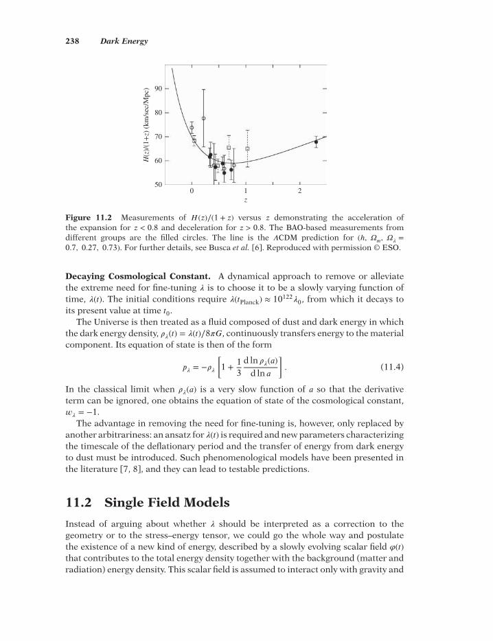
238 Dark Energy
90
80
H(z
)/(1
+z)
(km
/sec
/Mpc
)70
60
500 1
z2
Figure 11.2 Measurements of 𝐻(𝑧)∕(1 + 𝑧) versus 𝑧 demonstrating the acceleration ofthe expansion for 𝑧 < 0.8 and deceleration for 𝑧 > 0.8. The BAO-based measurements fromdifferent groups are the filled circles. The line is the 𝛬CDM prediction for (ℎ, 𝛺
𝑚, 𝛺
𝜆=
0.7, 0.27, 0.73). For further details, see Busca et al. [6]. Reproduced with permission © ESO.
Decaying Cosmological Constant. A dynamical approach to remove or alleviatethe extreme need for fine-tuning 𝜆 is to choose it to be a slowly varying function oftime, 𝜆(𝑡). The initial conditions require 𝜆(𝑡Planck) ≈ 10122
𝜆0, from which it decays toits present value at time 𝑡0.
The Universe is then treated as a fluid composed of dust and dark energy in whichthe dark energy density, 𝜌
𝜆(𝑡) = 𝜆(𝑡)∕8𝜋𝐺, continuously transfers energy to the material
component. Its equation of state is then of the form
𝑝𝜆= −𝜌
𝜆
[1 + 1
3d ln 𝜌
𝜆(𝑎)
d ln 𝑎
]. (11.4)
In the classical limit when 𝜌𝜆(𝑎) is a very slow function of 𝑎 so that the derivative
term can be ignored, one obtains the equation of state of the cosmological constant,𝑤
𝜆= −1.The advantage in removing the need for fine-tuning is, however, only replaced by
another arbitrariness: an ansatz for 𝜆(𝑡) is required and new parameters characterizingthe timescale of the deflationary period and the transfer of energy from dark energyto dust must be introduced. Such phenomenological models have been presented inthe literature [7, 8], and they can lead to testable predictions.
11.2 Single Field Models
Instead of arguing about whether 𝜆 should be interpreted as a correction to thegeometry or to the stress–energy tensor, we could go the whole way and postulatethe existence of a new kind of energy, described by a slowly evolving scalar field 𝜑(𝑡)that contributes to the total energy density together with the background (matter andradiation) energy density. This scalar field is assumed to interact only with gravity and
Single Field Models 239
with itself. In Section 7.2 we have already discussed this situation in the context ofsingle-field inflation.
Since a scalar field is mathematically equivalent to a fluid with a time-dependentspeed of sound, one can find potentials 𝑉 (𝜑) for which the dynamical vacuum acts likea fluid with negative pressure, and with an energy density behaving like a decayingcosmological constant. In comparison with plain 𝜆(𝑡) models, scalar field cosmologieshave one extra degree of freedom, since both a potential 𝑉 (𝜑) and a kinetic term 1
2��2
need to be determined.The simplest example of a minimally coupled and spatially homogeneous scalar
field has the Lagrangian density 5.86 and the equation of motion is then given by theKlein–Gordon Equation 7.24, where the prime indicates derivation with respect to 𝜑.
The energy density and pressure enter in the diagonal elements of 𝑇𝜇𝜈
, and they are
𝜌𝜑𝑐
2 = 12��
2 + 𝑉 (𝜑) and 𝑝𝜑= 1
2��
2 − 𝑉 (𝜑), (11.5)
respectively. Clearly the pressure is always negative if the evolution is so slow thatthe kinetic energy density 1
2��2 is less than the potential energy density. Note that in
Equations (7.24) and (11.5) we have ignored terms describing spatial inhomogeneitywhich could also have been present.
The conservation of energy-momentum for the scalar field is as in Equation (5.24),
��𝜑+ 3𝐻𝜌
𝜑(1 +𝑤
𝜑) = 0. (11.6)
As in Equation (5.29), the energy density of the scalar field decreases as 𝑎−3(1+𝑤
𝜑).
Inserting Equations (11.5) into Equation (11.6), one indeed obtains Equation (7.24).The equation of state of the 𝜑 field is then a function of the cosmological scale 𝑎 (ortime 𝑡 or redshift 𝑧),
𝑤𝜑= ��
2 + 2𝑉 (𝜑)��2 − 2𝑉 (𝜑)
. (11.7)
Starting early from a wide range of arbitrary initial conditions 𝑤𝜑
oscillates between≈ 1 and ≈ −1, until an epoch when 𝜌
𝜑freezes to a small value.
The conditions for acceleration are
𝑤𝜑< −1∕3, 𝑎(𝑡) ∝ 𝑡
𝑑 with d > 1
so that
𝑝𝜑< 0 or 𝜌
𝜑∝ 𝑎
−2.
However, dark energy defined this way and called quintessence turns out to beanother Deus ex machina which not only depends on the parametrization of an arbi-trary function 𝑉 (𝜑), but also has to be fine-tuned initially in a way similar to the cos-mological constant.
The Inflaton as Quintessence. Now we have met two cases of scalar fields causingexpansion: the inflaton field acting before 𝑡GUT and the quintessence field describingpresent-day dark energy. It would seem economical if one and the same scalar field

240 Dark Energy
could do both jobs. Then the inflaton field and quintessence would have to be matchedat some time later than 𝑡GUT. This seems quite feasible since, on the one hand, theinitially dominating inflaton potential 𝑉 (𝜑) must give way to the background energydensity 𝜌r + 𝜌m as the Universe cools, and on the other hand, the dark energy densitymust have been much smaller than the background energy density until recently.Recall that quintessence models are constructed to be quite insensitive to the initialconditions.
On the other hand, nothing forces the identification of the inflaton and quintessencefields. The inflationary paradigm in no way needs nor predicts quintessence.
In the previously described models of inflation, the inflaton field 𝜑 settled to oscil-late around the minimum 𝑉 (𝜑 = 0) at the end of inflation. Now we want the inflatonenergy density to continue a monotonic roll-down toward zero, turning ultimately intoa minute but nonvanishing quintessence tail. The global minimum of the potential isonly reached in a distant future, 𝑉 (𝜑 → ∞) → 0. In this process the inflaton does notdecay into a thermal bath of ordinary matter and radiation because it does not inter-act with particles at all, it is said to be sterile. A sterile inflaton field avoids violationof the equivalence principle, otherwise the interaction of the ultralight quintessencefield would correspond to a new long-range force. Entropy in the matter fields comesfrom gravitational generation at the end of inflation rather than from decay of theinflaton field.
The task is then to find a potential 𝑉 (𝜑) such that it has two phases of acceleratedexpansion: from 𝑡P to 𝑡end at the end of inflation, and from a time 𝑡F ≈ 𝑡GUT when theinstanton field freezes to a constant value until now, 𝑡0. Moreover, the inflaton energydensity must decrease faster than the background energy density, equalling it at sometime 𝑡∗ when the field is 𝜑∗, and thereafter remaining subdominant to the energy den-sity of the particles produced at 𝑡end. Finally it must catch up with a tracking potentialat some time during matter domination, 𝑡 > 𝑡eq.
The mathematical form of candidate potentials is of course very complicated, andit would not be very useful to give many examples here. However, it is instructive tofollow through the physics requirements on 𝜑 and 𝑉 (𝜑) from inflation to present.
Kination. Inflation is caused by an essentially constant potential 𝑉 (𝜑) according toEquation (7.36). The condition 𝑉 (𝜑 → ∞) → 0 requires an end to inflation at somefinite time 𝑡end when the field is 𝜑end and the potential is 𝑉end ≡ 𝑉 (𝜑end). The changein the potential at 𝑡end from a constant to a decreasing roll then implies, by Equa-tion (7.37), that ��end ≠ 0, and furthermore, by Equation (7.24), that also ��end ≠ 0. Thenthe slow-roll conditions in Equation (7.32) for 𝜖 and 𝜂 are also violated.
During inflation the kinetic energy density of the inflaton is
𝜌kin = 𝜖𝑉 =𝑚
2Planck
16𝜋
[𝑉
′2(𝜑)𝑉 (𝜑)
]. (11.8)
Thus when 𝑉 ′(𝜑) starts to grow, so does 𝜌kin. and the total energy density of the Uni-verse becomes dominated by the inflaton kinetic energy density. This epoch has been

Single Field Models 241
called kination or deflation. Equation (11.7) then dictates that the equation of state is
𝑤𝜑= ��
2 + 2𝑉 (𝜑)��2 − 2𝑉 (𝜑)
≈ 1, (11.9)
so that the kinetic energy density decreases as
𝜌(𝑎) ∝ 𝑎−3(1+𝑤) = 𝑎
−6 (11.10)
from Equation (5.29). This is much faster than the 𝑎−4 decrease of the radiationenergy density 𝜌r, and the 𝑎−3 decrease of the initially much smaller matter energydensity 𝜌m. Consequently, kination ends at the moment when 𝜌r overtakes 𝜌kin at time𝑡∗. When constructing phenomenological models for this scenario, one constraint isof course that 𝜌r(𝑡end) ≪ 𝑉end, or equivalently, 𝑡end < 𝑡∗. This behavior is well illustratedin Figure 11.3, taken from the work of Dimopoulos and Valle [9].
Since matter and radiation are gravitationally generated at 𝑡end, the reheating tem-perature of radiation is given by
𝑇reh = 𝛼𝑇H, (11.11)
where 𝑇H is the Hawking temperature [Equation (3.35)], and 𝛼 is some reheating effi-ciency factor less than unity. In Figure 11.3 the radiation energy density 𝜌
𝛾≡ 𝜌r starts
at 𝑇4reh
≪ 𝑉end, and then catches up with 𝑉 (𝜑) at 𝜑∗. Now the Universe becomes radia-tion dominated and the hot Big Bang commences. Note that the term ‘hot Big Bang’has a different meaning here: it does not refer to a time zero with infinite temperature,but to a moment of explosive entropy generation. This mimics the Big Bang so thatall of its associated successful predictions ensue.
Quintessence. The properties of the inflaton field plays no role any more during theBig Bang, they are fixed by requirements at Planck time when the quintessence fieldis completely negligible. The properties of quintessence, on the other hand, are fixedby present observations. This makes their identification rather artificial.
Let us continue the argument of the previous paragraph. The kinetic energy den-sity reduces rapidly to negligible,values by its 𝑎−6 dependence and the field freezesultimately to a nonzero value 𝜑F. The residual inflaton potential 𝑉 (𝜑) again starts todominate over the kinetic energy density, however, staying far below the radiationenergy density and, after 𝑡eq, also below the matter energy density.
As we approach 𝑡0, the task of phenomenology is to devise a quintessence potentialhaving a suitable tracker. The nature of the tracker potential is decided by the form ofthe quintessence potential. To arrive at the present-day dark energy which causes theevolution to accelerate, the field 𝜑 must be unfrozen again, so 𝜙F should not be verydifferent from 𝜙0. Many studies have concluded that only exponential trackers areadmissible, and that quintessence potentials can be constructed by functions whichbehave as exponentials in 𝜑 early on, but which behave more like inverse power poten-tials in the quintessential tail. A simple example of such a potential is
𝑉 (𝜑 ≫ 𝜑end) ≈ 𝑉endexp(−𝜆𝜑∕𝑚P)
(𝜑∕𝑚)𝑘, (11.12)

242 Dark Energy
V
T4reh
Vend
–4/3
–2
inflation kination HBB
ρkin
ργ
φend φFφ*
ρ
In ρ
–√2/3 λ
φ ≡ √3/2 ϕ/mp
Figure 11.3 Schematic view of the scalar potential from inflation to quintessence. The poten-tial 𝑉 (solid line) features two flat regions, the inflationary plateau and the quintessential tail.The inflation is terminated at 𝜑end by a drastic reduction of 𝑉 , leading to a rapid roll-downof the scalar field from the inflationary plateau towards the quintessential tail. At the end ofinflation the kinetic energy density of the scalar field, 𝜌kin (dash-dotted line), dominates for abrief period the energy density of the Universe. During this time the radiation energy density𝜌𝛾
(dashed line) reduces less rapidly and catches up with 𝜌kin at time 𝑡∗ when the field is 𝜑∗,and the explosive generation of entropy commences. After that the kinetic energy of the scalarfield reduces rapidly to zero and the field freezes asymptotically to a value 𝜑F, while the overallenergy density of the Universe (dash-dot-dotted line) continues to decrease due to the Hubbleexpansion. Assuming a quasi-exponential tail given by Equation (11.12), the potential beyond𝜑F is seen departing logarithmically from a pure exponential case (dotted line). Reprinted fromK. Dimopoulos and J. W. F. Valle, Modeling quintessential inflation [9], copyright 2002, withpermission from Elsevier.
where 𝑘 ⩾ 1 is an integer, 𝜆 > 0 is a parameter characterizing the exponential scale,and 𝑚 < 𝑚P is a mass scale characteristic of the adopted inverse power-law scale. Formore details, see Dimopoulos and Valle [9].
Tracking Quintessence. In a somewhat less arbitrary model [10, 11], one constructsquintessence in such a way that its energy density is smaller than the backgroundcomponent for most of the history of the Universe, somehow tracking it with the sametime dependence. This field converges onto the tracker solution with nearly constantslope −d ln 𝜌
𝜑∕d ln 𝑎 at a value < d ln 𝜌
𝑚∕d ln 𝑎, and regardless of the value of 𝑤
𝜑. in the
radiation-domination epoch, 𝑤𝜑
automatically decreases to a negative value at time𝑡eq when the Universe transforms from radiation domination to matter domination.

Single Field Models 243
We saw in Equation (5.33) that radiation energy density evolves as 𝑎−4—faster thanmatter energy density, 𝑎−3. Consequently, 𝜌r is now much smaller than 𝜌m.
But once 𝑤𝜑
is negative, 𝜌𝜑
decreases at a slower rate than 𝜌m so that it eventu-ally overtakes it. At that moment, 𝜑(𝑡) slows to a near stop, causing 𝑤
𝜑to decrease
toward −1, and tracking stops. Judging from the observed large value of the cosmo-logical constant density parameter today, 𝛺
𝜆= 0.714, this happened in the recent past
when the redshift was 𝑧 ∼ 2–4. Quintessence is already dominating the total energydensity, driving the Universe into a period of de Sitter-like accelerated expansion.
The tracker field should be an attractor in the sense that a very wide range of ini-tial conditions for 𝜑 and �� rapidly approach a common evolutionary track, so thatthe cosmology is insensitive to the initial conditions. Such cosmological solutions,called scaling solutions, satisfy 𝜌
𝜑(𝑡)∕𝜌m(𝑡) = constant > 0. Scaling solutions define the
borderline between deceleration and acceleration.Thus the need for fine-tuning is entirely removed, the only arbitrariness remains in
the choice of a function 𝑉 (𝜑). With a judicious choice of parameters, the coincidenceproblem can also be considered solved, albeit by tuning the parameters ad hoc.
In Chapter 7 we already discussed the inflationary de Sitter expansion followingthe Big Bang, which may also be caused by a scalar inflaton field. Here we just notethat the initial conditions for the quintessence field can be chosen, if one so desires,to match the inflaton field.
Tracking behavior with 𝑤𝜑< 𝑤b occurs [10, 11] for any potential obeying
𝛤 ≡ 𝑉′′𝑉 ∕(𝑉 ′)2 > 1, (11.13)
and which is nearly constant over the range of plausible initial 𝜑,
d(𝛤 − 1)𝐻 d𝑡
≪ |𝛤 − 1|, (11.14)
or if −𝑉 ′∕𝑉 is a slowly decreasing function of 𝜑. Many potentials satisfy these criteria,for instance power law, exponential times power law, hyperbolic, and Jacobian ellipticfunctions. For a potential of the generic form,
𝑉 (𝜑) = 𝑉0(𝜑0∕𝜑)−𝛽 (11.15)
with 𝛽 constant, one has a good example of a tracker field for which the kinetic andpotential terms remain in a constant proportion.
The values of 𝑤𝜑
and 𝛺𝜑
depend both on 𝑉 (𝜑) and on the background. The effectof the background is through the 3𝐻�� term in the scalar field equation of motion[Equation (7.24)] when 𝑤 changes, 𝐻 also changes, which, in turn, changes the rateat which the tracker field evolves down the potential.
The tracking potential is characterized as slow rolling when the slow-roll parame-ters [already defined in Equation (7.34)]
𝜂(𝜑) ≡𝑚
2Planck
16𝜋
(𝑉 ′′
𝑉
)≪ 1, 𝜖 ≡
𝑚2Planck
16𝜋
(𝑉 ′
𝑉
)2
≪ 1, (11.16)
meaning that �� in Equation (7.24) and ��2 in Equation (11.5) are both negligible. At
very early times, however, −𝑉′∕𝑉 is slowly changing, but is itself not small. This estab-
lishes the important distinction between static and quasi-static quintessence with

244 Dark Energy
𝑤𝜑≈ −1 and dynamical quintessence with 𝑤
𝜑> −1. This means that the slow-roll
approximation is not necessarily applicable to dynamical quintessence, and that thelatter generally requires exact solution of the equation of motion [Equation (7.24)].
Given a potential like Equation (11.15) and fixing the current values of parameters𝛺m, 𝛺r, 𝛺𝜑
, 𝑤𝜑
one can solve the equation of motion [Equation (7.24)] by numericalintegration. Finding the functions 𝛤 (𝑎), 𝑤
𝜑(𝜑), 𝑤
𝜑(𝑎) or 𝛺
𝜑(𝑎) is a rather complicated
exercise. Finally, when the potential gets shallow, the relatively fast-rolling dynamicalquintessence solution exits from the scaling regime and becomes static, approachingthe 𝑤
𝜑= −1 regime, and an accelerated expansion commences.
The equation of state of dark energy, 𝑤𝜑, introduces a new degeneracy with 𝛺m and
ℎ which cannot be resolved by CMB data alone. Using the full set of available data inFigure 9.1, one can obtain limits to 𝑤
𝜑.
In this model the lookback time is given by
𝑡(𝑧) = 1𝐻0 ∫
1∕(1+𝑧)
1d𝑎
[(1 −𝛺0) +𝛺m𝑎
−1 +𝛺r𝑎−2 +𝛺
𝜑𝑎
2−3(1+𝑤𝜑)]−1∕2
. (11.17)
For 1∕(1 + 𝑧) = 0 this gives us the age [Equation (5.55)] of the Universe, 𝑡0.For the case of −1 < 𝑤
𝜑, the effect on galaxy formation is earlier collapse times
and more rapid collapse of overdensities. The equation of state and the amplitudeof velocity fluctuations 𝜎8 are correlated in such a way that for constant 𝑤
𝜑, higher
(lower) 𝜎8 produces earlier (later) collapse times, respectively.
K-Essence. As already mentioned, the weakness of the tracking quintessence modelis that the energy density for which the pressure becomes negative is set by anadjustable parameter which has to be fine-tuned to explain the cosmic coincidence.Surely one can do better by adding degrees of freedom, for instance by letting 𝜑(𝑡)interplay with the decaying cosmological constant 𝜆(𝑡), or with the matter field, orwith a second real scalar field 𝜓(𝑡) which dominates at a different time, or by taking𝜑(𝑡) to be complex, or by choosing a double-exponential potential, or by adding a newtype of matter or a dissipative pressure to the background energy density. Surely thepresent acceleration could have been preceded by various periods of deceleration andacceleration. These are only a few of the alternatives that have been proposed.
One interesting alternative called K-essence [12] comes at the cost of introducing anonlinear kinetic energy density functional of the scalar field. In Equation (5.86) weintroduced a Lagrangian which we now slightly generalize to read
phi,𝑋 = 12𝑔𝜇𝜈𝜕𝜇𝜙𝜕
𝜈𝜙 − 𝑉 (𝜙) ≡ 𝑋 − 𝑉 (𝜑). (11.18)
𝑋 could be replaced by a a positive semi-definite kinetic function of 𝐾(𝑋).If 𝜑 describes a perfect fluid with pressure 𝑝 and density 𝜌k the energy-momentum
tensor is given by 𝑝 = and
𝜌k = [2𝑋𝐾′(𝑋) −𝐾(𝑋)] + 𝑉 (𝜑) (11.19)
where a prime denotes a partial derivative with respect to 𝑋. Then 𝑤𝜑≡ 𝑝∕𝜌. A nec-
essary condition that the theory be stable is 𝜌 > 0 and further that the speed of sound𝜕𝑝∕𝜕𝜌 be positive.

Single Field Models 245
Solving the equations one finds that the solution is tracking, just like quintessence.It is also quite insensitive to the initial conditions. The K-field tracks the radiationenergy density until 𝑡eq, when a sharp transition from positive to negative pressureoccurs, with 𝑤
𝜑= −1 as a consequence. The K-essence density 𝜌k then drops below
𝜌m and, thereafter, in the matter-dominated epoch the K-field does not track the back-ground at all, it just stays constant. Thus the time of K-essence domination and accel-erated expansion simply depends on 𝑡eq. However, this is another case of fine-tuning:𝜌k must drop precisely to the magnitude of the present-day 𝜌
𝜆.
Phantom Fields. Could the scalar field obey an equation of state with negativekinetic energy violating the weak energy condition 𝜌 + 𝑝 ⩾ 0?. This can occur in manymodels but one is trying to avoid it at all costs. The reason for this is serious problemswith quantum instabilities. Since 𝑤
𝜑< −1, such a universe evolves within a finite time
to a Big Rip singularity when the curvature grows toward ∞.However, the singularity can be avoided if the potential has a maximum, for
instance
𝑉 (𝜑) =𝑉0
cosh (𝜑∕𝜑0). (11.20)
In contrast to ordinary kinematics, the phantom field evolves toward the top of thepotential and crosses over on the other side. It then turns around and again returns tothe top, executing damped oscillations across the top until it finally settles at 𝑤
𝜑= −1.
This model is strongly disfavored by the data in comparison with genuine 𝑤𝜑= −1
models.
Tachyon Fields. Somewhat related are tachyon fields which move with superlu-minal velocity. Since special relativity in four-dimensional spacetime forbids this,tachyon models require rather drastic revisions of general relativity or of spacetime.Speculations have also appeared in the literature that the Universe might have under-gone shorter periods of this type. It is well to remember that nothing is known aboutwhether the cosmological constant is indeed constant or whether it will remain so,nor about the future behavior of a quintessence field and its equation of state.
In higher-dimensional spacetimes tachyons may move in the bulk between ourfour-dimensional brane and other branes. The potential may be of the form 11.20so that the field has a ground state at 𝑤
𝜑= ∞.
In a flat FRW background one has
𝜌𝜑= 𝑉 (𝜑)√
1 − (��2)and 𝑝
𝜑= −𝑉 (𝜑)2
𝜌𝜑
. (11.21)
From Friedmann’s equations one then obtains
��
𝑎= 8𝜋𝐺
3𝑉 (𝜑)√1 − ��2
(1 − 2��2). (11.22)
Hence the accelerated expansion occurs for ��2< 2∕3. Note that 𝑤
𝜑= ��
2 − 1 is in therange −1 < 𝑤
𝜑< 0.

246 Dark Energy
Chaplygin Gas. Another simple and well-studied model of dark energy introducesinto 𝑇
𝜇𝜈the density 𝜌
𝜑and pressure 𝑝
𝜑of an ideal fluid with a constant potential
𝑉 (𝜑) = 𝐴 > 0 called Chaplygin gas following Chaplygin’s historical work in aerodynam-ics. Here 𝐴 has the dimensions of energy density squared. Ordinary matter is assumednot to interact with Chaplygin gas, therefore one has separate continuity equations forthe energy densities 𝜌
𝑚and 𝜌
𝜑of the same form as in FLRW geometry, respectively,
�� + 3𝐻(𝜌 + 𝑝) = 0. (11.23)
Pressureless dust with 𝑝 = 0 then evolves as 𝜌𝑚(𝑎) ∝ 𝑎−3.
The barotropic equation of state is
𝑝𝜑= −𝐴∕𝜌
𝜑. (11.24)
The continuity Equation (11.23) is then
��𝜑+ 3𝐻(𝜌
𝜑− 𝐴∕𝜌
𝜑) = 0,
which integrates to
𝜌𝜑(𝑎) =
√𝐴 + 𝐵∕𝑎6, (11.25)
where 𝐵 is an integration constant. Thus this model has two free parameters.Obviously the limiting behavior of the energy density is
𝜌𝜑(𝑎) ∝
√𝐵
𝑎3for 𝑎 ≪
(𝐵
𝐴
)1∕6, 𝜌
𝜑(𝑎) ∝
√𝐴 for 𝑎 ≫
(𝐵
𝐴
)1∕6. (11.26)
At early times this gas behaves like pressureless dust, like CDM, at late times itbehaves like the cosmological constant, causing accelerated expansion. The problemis, that when the dust effect disappears but CDM remains, this causes a strong ISWeffect and loss of CMB power, thus the model is a poor fit to data (SNe, BAO, CMB).To remedy this one has complicated the model by adding a new parameter, 𝛽, to thebarotropic equation of state:
𝑝𝜑= −𝐴∕𝜌𝛽
𝜑. (11.27)
Unfortunately, the fit then approaches the standard cosmological constant solution.
11.3 𝒇 (𝑹) Models
In Section 5.5 we have already met models of modified gravity which are candidatesboth for inflation and for the present accelerated expansion.
In Equation (5.85) we replaced the curvature scalar 𝑅 by a general function 𝑓 (𝑅,𝜑),and enlarged the dimensionality of space-time from 4 to 𝑛.
The Einstein–Hilbert action is not renormalizable, therefore standard general rel-ativity cannot be properly quantized. However, renormalizability can be cured byadding higher order terms in curvature invariants. This is similar to the situationin quantum field theory where renormalization is some procedure to remove infinitiesin calculations. If the Lagrangian contains combinations of field operators of high

𝒇 (𝑹) Models 247
enough dimension in energy units, the counterterms required to cancel all divergencesproliferate to infinite number, and, at first glance, the theory would seem to gain aninfinite number of free parameters and therefore lose all predictive power, becomingscientifically worthless. Such theories are called nonrenormalizable.
The Standard Model of particle physics contains only renormalizable operators,but the interactions of general relativity become nonrenormalizable operators if oneattempts to construct a field theory of quantum gravity in the most straightforwardmanner, suggesting that perturbation theory is useless in applications to quantumgravity.
The endeavor to remedy the renormalizability of the Einstein–Hilbert actionimplies adding functions of the Ricci scalar 𝑅 which become important at late timesand for small values of the curvature. This is required in order to avoid conflicts withconstraints from the solar system or the Galaxy.
Consider an action of the form
𝑆 ∝[∫
d4𝑥√−𝑔[𝑅 + 𝑓 (𝑅)] +
∫d4
𝑥√−𝑔
𝑚(𝑔
𝜇𝜈, 𝛹 )
](11.28)
where 𝑓 (𝑅) is an unspecified function of 𝑅. The matter Lagrangian 𝑚
is minimallycoupled and, therefore the matter fields 𝛹 fall along the metric 𝑔
𝜇𝜈. By varying this
action with respect to 𝑔𝜇𝜈
one can obtain the field equations of the form
��𝜇𝜈
≡ 𝑅𝜇𝜈
− 12𝑅𝑔
𝜇𝜈−𝑄
𝜇𝜈(11.29)
where ��𝜇𝜈
contains the modifications to the geometry in terms of the functions𝑓 (𝑅), 𝑓
𝑅≡ 𝜕𝑓∕𝜕𝑅, 𝑔
𝜇𝜈. The 𝑓 (𝑅) term leads to extra terms in the Einstein equation
which is of second order in the metric 𝑔𝜇𝜈
. The constraint equation of GR becomesa third order equation, and the evolution equations now become fourth order dif-ferential equations which are difficult to analyze. A more tractable form of extendedgravity can be obtained by using the Palatini variation, briefly discussed at the end ofChapter 5.
When taking the metric to be of the Robertson–Walker form [Equation (2.32)] theFriedmann equation becomes
𝐻2 + 𝑓
6− ��
𝑎𝑓𝑅+𝐻 𝑓
𝑅= 𝜅
2𝜌
3(11.30)
where 𝑓 ≡ 𝑓 (𝑅). The Raychauduri equation becomes
��
𝑎− 𝑓
𝑅𝐻
2 + 𝑓
6+
𝑓𝑅
2= −𝜅2
6(𝜌 + 3𝑝) (11.31)
and the stress-energy tensor is replaced by
��𝜇𝜈
=𝑇𝜇𝜈
𝑓𝑅
. (11.32)
Any 𝑓 (𝑅) theory designed to achieve cosmic acceleration must satisfy |𝑓 ≪ 𝑅| and|𝑓
𝑅| ≪ 1 at high curvature to be consistent with our knowledge of the high redshift
universe. In order for 𝑓𝑅
not to be tachyonic it must have a positive squared mass,that is, there must exist a stable high-curvature regime, such as a matter dominated

248 Dark Energy
universe 𝑓RR > 0 for 𝑅 ≫ 𝑓RR. Further requirements are 1 + 𝑓𝑅> 0 for all finite 𝑅 (this
prevents the graviton from becoming ghost-like), 𝑓 (𝑅)∕𝑅 → 0 and 𝑓𝑅→ 0 as 𝑅 → ∞
(GR must be recovered early before the BBN and the CMB), and 𝑓𝑅
must be small atrecent epochs [13]. The condition for an accelerated expansion is 𝑎(𝑡) ∝ 𝑡𝑑 with 𝑑 > 1,suitable also for the exponential quintessence potential.
An example of a good potential is
𝑓 (𝑅) = 𝑅
⎡⎢⎢⎣1 + 𝛼
(− 𝑅
𝐻20
)𝛽−1⎤⎥⎥⎦(11.33)
with 𝛼 and 𝛽 constants, and which describes well the radiation-dominated era, thematter-dominated era, and the present accelerated era, but not the inflation. In thelimit 𝑅 = 0 one has flat geometry and standard GR.
Higher Order Invariants. Nothing forbids one to complement the Ricci scalar 𝑅
with invariants of higher order in curvature. The advantage is that they introduceextra degrees of freedom, but they may come at a cost. They can lead to instabilitiesand conflicts with local tests of gravity. The invariants of lowest mass dimension are
𝑃 ≡ 𝑅𝜇𝜈𝑅
𝜇𝜈𝑄 ≡ 𝑅
𝛼𝛽𝛾𝛿𝑅
𝛼𝛽𝛾𝛿. (11.34)
which have actions similar to Equation (11.27),
𝑆 ∝[∫
d4𝑥√−𝑔[𝑅 + 𝑓 (𝑅, 𝑃 , 𝑄)] +
∫d4
𝑥√−𝑔
𝑚(𝑔
𝜇𝜈, 𝛹 )
]. (11.35)
The equations of motion can again be found by varying this action with respectto 𝑔
𝜇𝜈.
The combination of invariants that seems most promising and is most studied is𝑅
2 − 4𝑃 +𝑄, called the Gauss–Bonnet term.
11.4 Extra Dimensions
Already the generalized form of the Einstein–Hilbert action [Equation (5.85)] allowedfor the possibility of a spacetime of 𝑛 > 4 dimensions. Let us assume that the observ-able physics occurs on a four-dimensional brane embedded in a five-dimensionalMinkowski bulk universe. Gravitation occurs everywhere in this bulk, but at cosmo-logically late times (now) it gets weaker on the brane, it leaks out into the bulk outsideour brane, causing the present accelerated expansion.
The DGP model. A simple and well-studied model of modified gravity in five space-time dimensions is the Dvali–Gabadadze–Porrati (DGP) braneworld model. The modelis characterized by a cross-over scale 𝑟
𝑐such that gravity is a four-dimensional theory
at scales 𝑎 ≪ 𝑟𝑐𝐻0 where matter behaves as pressureless dust. In the self-accelerating
DGP branch, gravity ‘leaks out’ into the bulk when 𝑎 ≈ 𝑟𝑐𝐻0, and at scales 𝑎 ≫ 𝑟
𝑐𝐻0 the
model approaches the behavior of a cosmological constant. To explain the accelerated

Extra Dimensions 249
expansion which is of recent date (𝑧 ≈ 0.7 or 𝑎 ≈ 0.6), 𝑟𝑐𝐻0 must be of the order
of unity. In the self-decelerating DGP branch, gravity ‘leaks in’ from the bulk atscales 𝑎 ≈ 𝑟
𝑐𝐻0, in conflict with the observed dark energy acceleration. Note that
the self-accelerating branch has a ghost, whereas the self-decelerating branch isghost-free.
On the four-dimensional brane the action of gravity is proportional to 𝑀2Pl
whereasin the bulk it is proportional to the corresponding quantity in five dimensions, 𝑀
35 .
The cross-over length is defined as
𝑟𝑐= 𝑀
2Pl∕2𝑀3
5 . (11.36)
It is customary to associate a density parameter to this,
𝛺𝑟𝑐
= (2𝑟𝑐𝐻0)−2
, (11.37)
such that 𝑟𝑐𝐻0 is a length scale (similar to 𝑎).
The Friedmann–Lemaitre equation may be written
𝐻2 + 𝑘
𝑎2− 𝜖
1𝑟 𝑐
√𝐻2 + 𝑘
𝑎2= 𝜅𝜌, (11.38)
where 𝑎 = (1 + 𝑧)−1, 𝜅 = 8𝜋𝐺∕3, and 𝜌 is the total cosmic fluid energy density withcomponents 𝜌
𝑚for baryonic and dark matter, and 𝜌
𝜑for whatever additional dark
energy may be present.Clearly the standard FLRW cosmology is recovered in the limit 𝑟
𝑐→ ∞ or 𝐻 ≪ 𝑟
𝑐.
When 𝐻 ⩾ 𝑟𝑐
the root term becomes important. In flat-space geometry 𝑘 = 0, and atlate times when 𝜌 ∝ 1∕𝑎3 → 0 and 𝐻 → 𝐻∞ this becomes a de Sitter acceleration, 𝑎(𝑡) ∝exp 𝑡∕𝑟
𝑐.
The self-accelerating branch corresponds to 𝜖 = +1, the self-decelerating branch to𝜖 = −1. In DGP geometry the continuity equations for ideal fluids have the same formas in FLRW geometry [Equation (11.28)].
Pressureless dust with 𝑝 = 0 then evolves as 𝜌𝑚(𝑎) ∝ 𝑎−3. The free parameters in the
DGP model are 𝛺𝑟𝑐
and 𝛺𝑚= 𝜅𝜌
𝑚∕𝐻2
0 . Note that there is no curvature term 𝛺𝑘
sincewe have assumed flatness by setting 𝑘 = 0 in Equation (11.33).
In the space of the parameters 𝛺k, 𝛺m and 𝛺𝑟𝑐≡ 1∕4𝑟2
𝑐𝐻
20 one can generalize the
DGP model to
𝐻2 − 𝑘
𝑎2− 𝑟
−2𝑐
(𝑟𝑐
√𝐻2 − 𝑘
𝑎2
)2−𝑛
= 𝜅𝜌, (11.39)
where 𝑛 defines a parametric family. Comparisons with data show that 𝑛 = 1 and 𝑛 > 3give poor fits, 𝑛 = 2 corresponds to the 𝜆CDM concordance model, and 𝑛 = 3 givesgood fits.
The Chaplygin–DGP Model. Both the self-accelerating DGP model and the stan-dard Chaplygin gas model have problems fitting present observational data, bothcause too much acceleration. They have at least one parameter more than 𝜆CDM,yet they fit data best in the limit where they reduce to 𝜆CDM.

250 Dark Energy
Because of the similarities in the asymptotic properties of the two-parametric DGPmodel and the two-parametric Chaplygin gas model. I have proposed [13] to combinethe self-decelerating branch of the DGP model with the accelerating Chaplygin gasmodel. There are then four free parameters, 𝛺
𝑟𝑐
, 𝛺𝑚, 𝐴, and 𝐵, one of which shall be
eliminated shortly.We now choose the length scales in the two models, 𝑟
𝑐𝐻0 and (𝐵∕𝐴)1∕6, to be pro-
portional by a factor 𝑥, so that(𝐵
𝐴
)1∕6= 𝑥𝑟
𝑐𝐻0 = 𝑥
2√
𝛺𝑟𝑐
. (11.40)
The proportionality constant subsequently disappears because of a normalizing con-dition at 𝑧 = 0. Then the model has only one parameter more than the standard 𝛬CDMmodel.
It is convenient to replace the parameters 𝐴 and 𝐵 in Equation (11.40) by two new
parameters, 𝛺𝐴= 𝐻
−20 𝜅
√𝐴 and 𝑥 = 2
√𝛺
𝑟𝑐(𝐵∕𝐴)1∕6. The dark energy density can then
be written
𝜌𝜑(𝑎) = 𝐻
20𝜅
−1𝛺
𝐴
√1 + 𝑥6(4𝛺
𝑟𝑐𝑎2)−3. (11.41)
Let us now return to Equation (11.38) and solve it for the expansion history 𝐻(𝑎).Substituting 𝛺
𝑟𝑐from Equation (11.37), 𝜌
𝜑(𝑎) from Equation (11.41), and using 𝛺
𝑚=
𝛺0𝑚𝑎−3, it becomes
𝐻(𝑎)𝐻0
= −√
𝛺𝑟𝑐
+[𝛺
𝑟𝑐
+𝛺0𝑚𝑎−3 +𝛺
0𝑟𝑎−4 +𝛺
𝐴
√1 + 𝑥6(4𝛺
𝑟𝑐
𝑎2)−3]1∕2
. (11.42)
Note that 𝛺𝑟𝑐
and 𝛺𝐴
do not evolve with 𝑎, just like 𝛺𝜆
in the the 𝜆CDM model. In thelimit of small 𝑎 this equation reduces to two terms which evolve as 𝑎
−3∕2, somewhat
similarly to dust with density parameter√
𝛺0𝑚 +𝛺
𝐴𝑥3(4𝛺
𝑟𝑐)−3∕2.
In the limit of large 𝑎, Equation (11.42) describes a de Sitter acceleration with a
cosmological constant 𝛺𝜆= −
√𝛺
𝑟𝑐
+√
𝛺𝑟𝑐
+𝛺𝐴.
A closer inspection of Equation (11.42) reveals that it is not properly normalizedat 𝑎 = 1 to 𝐻(1)∕𝐻0 = 1, because the right-hand-side takes different values at differentpoints in the space of the parameters 𝛺
0𝑚, 𝛺
𝑟𝑐
, 𝛺𝐴
, and 𝑥. This gives us a condition: at𝑎 = 1 we require that 𝐻(1) = 𝑥𝐻0 so that Equation (11.42) takes the form of a sixthorder algebraic equation in the variable 𝑥
𝑥 = −√
𝛺𝑟𝑐+[𝛺
𝑟𝑐+𝛺
0𝑚+𝛺
𝐴
√1 + 𝑥6(4𝛺
𝑟𝑐)−3
]1∕2. (11.43)
This condition shows that 𝑥 is a function 𝑥 = 𝑓 (𝛺0𝑚,𝛺
𝑟𝑐
, 𝛺𝐴). Finding real, positive
roots 𝑥 and substituting them into Equation (11.42) would normalize the equationproperly. The only problem is that the function cannot be expressed in closed form,so one has to resort to numerical iterations. The average value of 𝑥 is found to be 𝑥 ≈0.956; it varies over the interesting part of the parameter space, but only by ≈ 0.002.
This model [13] fits SNeIa data with the same goodness of fit as the the cosmologicalconstant model, it also fits the CMB shift parameter 𝑅 well, and notably, it offers a

Extra Dimensions 251
genuine alternative to the cosmological constant model because it does not reduce toit in any limit of the parameter space.
The Gauss–Bonnet Model. Consider an action in a six-dimensional spacetime ofthe form
𝑆 ∝[∫
d6𝑥√−𝑔(𝑅 + 𝜖GB)
](11.44)
where 𝜖 is the Gauss–Bonnet (GB) parameter. Only 𝜖 > 0 yields accelerating solutions.The metric consists of two pieces, the FRW metric and the GB metric,
d𝑠2 = 𝑐2 d𝑡2 − 𝑎(𝑡)2d𝑙 2
FRW − 𝑏(𝑡)2[(d𝑥4)2 + (d𝑥5)2]. (11.45)
The FRW Hubble flow and acceleration are the standard ones, 𝐻 = ��∕𝑎 and �� ,respectively. The GB Hubble flow is ℎ = ��∕𝑏 and the GB acceleration is ℎ. The modelhas (at least) two interesting solutions:
(i) In GB space there is decreasing deceleration, ℎ < 0, towards a stop when ℎ = 0.With time, the FRW behavior starts to dominate. In FRW space the expansion𝐻 and acceleration �� > 0 continue until a future singularity as in de Sitterexpansion.
(ii) 𝐻 and ℎ oscillate around future values of expansion and contraction. In FRWspace there is almost no acceleration, �� ≈ 0. In GB space ℎ oscillates betweenacceleration and deceleration, finally arriving at a future fixed point.
Lemaitre–Tolman-Bondi Models. A way to explain the dimming of distant super-novae without dark energy may be an inhomogeneous universe described by theLemaıtre–Tolman–Bondi solution (LTB) to Einstein’s equation. We could be locatednear the center of a low-density void which would distort our measurements of the ageof the Universe, the CMB acoustic scale, and the Baryon Acoustic Oscillations (BAO).
The LTB model describes general radially symmetric spacetimes in four dimen-sions. The metric can be described by
𝑑𝑠2 = −𝛼
2𝑑𝑡
2 +𝑋2(𝑟, 𝑡) 𝑑𝑟2 + 𝐴
2(𝑟, 𝑡) 𝑑𝛺2, (11.46)
where 𝑑𝛺2 = 𝑑𝜃2 + si𝑛2𝜃𝑑𝜑2, 𝐴(𝑟, 𝑡) and 𝑋(𝑟, 𝑡) are scale functions, and 𝛼(𝑡, 𝑟) > 0 is thelapse function.
Assuming a spherically symmetric matter source with baryonic+dark matter den-sity 𝜌
𝑀, dark energy density 𝜌DE, negligible matter pressure 𝑝
𝑀= 0 and dark energy
pressure density 𝑝DE, the stress-energy tensor is
𝑇𝜇
𝜈 = 𝑝DE 𝑔𝜇
𝜈 + (𝜌𝑀
+ 𝜌DE + 𝑝DE) 𝑢𝜇𝑢𝜈. (11.47)
The (0, 𝑟) components of Einstein’s equations, 𝐺0𝑟= 0, imply
��(𝑡, 𝑟)2[1 − 𝑘(𝑡, 𝑟)]
+ 𝛼′��
𝛼𝐴′ = 0 (11.48)
with an arbitrary function 𝑘(𝑡, 𝑟) playing the rôle of the spatial curvature parameter.Here an overdot is designating 𝜕
𝑡and an apostrophe 𝜕
𝑟.

252 Dark Energy
The 𝑇00 component of Einstein’s equations gives the Friedmann–Lemaıtre equation
in the LTB metric [Equation (11.46)]
𝐻2𝑇
𝛼2+
2𝐻𝑇𝐻
𝐿
𝛼2+ 𝑘
𝐴2+ 𝑘′(𝑡, 𝑟)
𝐴𝐴′ = 8𝜋𝐺 (𝜌𝑀
+ 𝜌DE). (11.49)
Here 𝐻𝑇= ��∕𝐴 is the transversal Hubble expansion, 𝐻
𝐿= ��′∕𝐴′ the longitudinal Hub-
ble expansion.The 𝑇 𝑟
𝑟components of Einstein’s equations give
2��𝑇+ 3𝐻2
𝑇+ 𝑘
𝐴2− 8𝜋𝐺 𝑝DE = 0. (11.50)
Multiplying each term with 𝐴3 𝐻𝑇
this can be integrated over time to give
𝐻2𝑇= 𝐹 (𝑟)
𝐴3− 𝑘(𝑟)
𝐴2− 8𝜋𝐺
𝐴3 ∫dt𝐴3
𝐻𝑇𝑝DE. (11.51)
Here 𝐹 (𝑟) is an arbitrary time-independent function which arose as an integrationconstant.
We now assume that dark energy does not interact with matter. There are then sep-arate continuity equations for ordinary matter and dark energy. The one for matter is
��𝑀(𝑟, 𝑡) + [2𝐻
𝑇(𝑟, 𝑡) +𝐻
𝐿(𝑟, 𝑡)] 𝜌
𝑀(𝑟, 𝑡) = 0, (11.52)
and it can be integrated to give
𝜌𝑀(𝑟, 𝑡) = 𝐹 (𝑟)
𝐴2𝐴′(11.53)
The continuity equation for dark energy is
��DE(𝑟, 𝑡) + [2𝐻𝑇(𝑟, 𝑡) +𝐻
𝐿(𝑟, 𝑡)] [𝜌DE(𝑟, 𝑡) + 𝑝DE(𝑟, 𝑡)] = 0. (11.54)
To proceed we should now specify several arbitrary functions, so we leave the sub-ject here unfinished.
Problems
1. Derive Equation (5.76).
2. What should 𝑡eq be for K-essence 𝜌k to drop precisely to the magnitude of thepresent-day 𝜌
𝜆≈ 2.9 × 10−47 GeV4?
3. Suppose that dark energy is described by an equation of state 𝑤 = −0.9 which isconstant in time. At what redshift did this dark energy density start to dominateover matter density? What was the radiation density at that time?
4. Derive this expression for the K-essence energy density:
𝜌k = [2𝑋𝐾′(𝑋) −𝐾(𝑋)] + 𝑉 (𝜑)
5. Derive the field equations for an action of the form in Equation (11.28) with𝑓 (𝑅) = 𝑅2. The ordinary matter part
𝑚can be ignored.

Extra Dimensions 253
References[1] Riess, A. G. et al. 1998 Astronom. J. 116, 1009.[2] Perlmutter, S. et al. 1998 Nature 391, 51; 1999 Astrophys. J. 517, 565.[3] de Bernardis, F. et al. 2000 Nature 404, 955.[4] Hanany, S. et al. 2000 Astrophys. J. Lett. 545, L5.[5] Farook, O. and Ratra, B. 2013 Astrophys. J. Lett. 766. L7.[6] Busca, N. G. et al. 2012 Astron. Astrophys 552, A96.[7] Lima, J. A. S. and Trodden, M. 1996 Phys. Rev. D 53, 4280.[8] Cunha, J. V., Lima, J. A. S. and Pires, N. 2002 Astron. Astrophys. 390, 809.[9] Dimopoulos, K. and Valle, J. W. F. 2002 Astroparticle Phys. 18, 287.
[10] Steinhardt, P. J., Wang, L. and Zlatev, I. 1999 Phys. Rev. D, 59, 123504.[11] Zlatev, I., Wang, L. and Steinhardt, P. J. 1999 Phys. Rev. Lett. 82, 896.[12] Armendariz-Picon, C., Mukhanov, V. and Steinhardt, P. J. 2000 Phys. Rev. Lett. 85, 4438;
2001 Phys. Rev. D, 63, 103510.[13] Roos, M. 2008 Phys. Letters B 666, 420.


12
Epilogue
We have now covered most of cosmology briefly, starting from the theoretical scenar-ios in Figure 5.1 and arriving at Figure 12.1, where the scenarios have been populatedby data which permit a selection. Thus we know now that the cosmic expansion isaccelerated since recently, since the time corresponding to redshift 𝑧 ≈ 0.8. But westill do not know what causes the acceleration—therefore the mysterious term ‘darkenergy’, which represents 71.4% of the energy density of the Universe. In Chapter 11we met a multitude, albeit not exhaustive set of candidates. The observational knowl-edge has improved greatly, but the solution remains unknown. The simplest candi-date, the cosmological constant 𝜆, begs an answer as to its origin and its value whichhas to be fine-tuned to within the 52nd decimal of zero (in units of 𝑐 = 1). Determi-nations of the equation of state of dark energy, 𝑤, point to phantom models, but thecosmological constant value 𝑤 = −1 is still close to the 1𝜎 contour, see Figure 8.7 andthe cover of this book.
The knowledge of the equally mysterious dark matter has gone from a disbelievedcuriosity in 1933 to the important field of study today described in Chapter 8, muchthanks to the enormous development in gravitational lensing. It represents 23.4% ofthe energy density of the Universe, yet its composition is unknown, except that it iscold. What has happened most recently is, that the long favored WIMP candidateshave reached the useful search limit, and that the minimal supersymmetry modelappears unlikely. In any case one should keep in mind, that the discovery of a newparticle in a terrestrial accelerator does not prove that it is dark matter. That shouldbe discovered at galactic scales.
Cosmic inflation is a field of vigorous study, but we are still relying on essentiallythe same model as 20 years ago, as described in Section 7.2. One should construct arenormalized field theory of quantum gravity to cope with the initial Big Bang singu-larity and inflation, but that is beyond the level of this monography. Models of infla-tion will be tested in the near future with the advent of more and better evidence forgravitational waves.
Introduction to Cosmology, Fourth Edition. Matts Roos© 2015 John Wiley & Sons, Ltd. Published 2015 by John Wiley & Sons, Ltd.

256 Epilogue
0 0.5 1 1.5 2
Redshift z
–0.5
0
0.5
1
Δ (m
-M)
always accelerates
accelerates nowdecelerates in the past
always decelerates
flatopen
closed
Figure 12.1 Evidence for transition from deceleration in the past to acceleration today. Thedifference m–M is defined in Equation (2.60). The blue line shows a model that fits the data,where acceleration happens at late epochs in the history of the universe (i.e. starting a fewbillion years ago, and billions of years after the Big Bang). The plot uses binned data from theUnion2 compilation [2]. With permission from the author. (See plate section for color version.)
Occasionally we have had reason to discuss a universe with extra dimensions: thecyclic universe in Section 7.4, some models of dark energy in Section 11.4. Theyremain candidates.
The future will bring great improvements in observational capacity, as we havewitnessed ever since COBE, so cosmology will remain an active and fascinating field.
I thank the reader for her/his patience to come to this sentence!
References[1] Huterer, D. 2011 Adventures in Cosmology, ed. D. Goodstein, World Scientific Pub. Co., and
preprint arXiv:1010.1162 [astro-ph.CO].[2] Amanullah, R. et al. 2010 Astrophys. J. 716, 712.

Tables
Table A.1 Cosmic distances and dimensions
Distance to the Sun 8′ 15′′ (light minutes)Distance to the nearest star (𝛼 Centauri) 1.3 pcDiameters of globular clusters 5–30 pcThickness of our Galaxy, the ‘Milky Way’ 0.3 kpcDistance to our galactic center 8 kpcRadius of our Galaxy, the ‘Milky Way’ 12.5 kpcDistance to the nearest galaxy (Large Magellanic Cloud) 55 kpcDistance to the Andromeda nebula (M31) 770 kpcSize of galaxy groups 1–5 MpcThickness of filament clusters 5ℎ−1 MpcDistance to the Local Supercluster center (in Virgo) 17 MpcDistance to the ‘Great Attractor’ 79ℎ−1 MpcSize of superclusters ≳ 50ℎ−1 MpcSize of large voids 60ℎ−1 MpcDistance to the Coma cluster 100ℎ−1 MpcLength of filament clusters 100ℎ−1 MpcSize of the ‘Sloan Great Wall’ 420 ℎ−1 MpcHubble radius 3000ℎ−1 Mpc
Introduction to Cosmology, Fourth Edition. Matts Roos© 2015 John Wiley & Sons, Ltd. Published 2015 by John Wiley & Sons, Ltd.
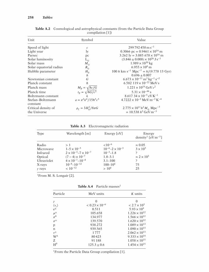
258 Tables
Table A.2 Cosmological and astrophysical constants (from the Particle Data Groupcompilation [1])
Unit Symbol Value
Speed of light 𝑐 299 792 458 m s−1
Light year ly 0.3066 pc = 0.9461 × 10¹⁶ mParsec pc 3.262 ly = 3.085 678 × 1016 mSolar luminosity L
⊙(3.846 ± 0.008) × 1026 J s−1
Solar mass 𝑀⊙
1.989 × 1030 kgSolar equatorial radius 𝑅
⊙6.955 × 10⁸ m
Hubble parameter 𝐻0 100 ℎ km s−1 Mpc−1 = ℎ∕(9.778 13 Gyr)ℎ 0.696 ± 0.007
Newtonian constant 𝐺 6.673 × 10⁻¹¹ m3 kg−1 s−2
Planck constant ℏ 6.582 119 × 10−22 MeV sPlanck mass 𝑀P =
√ℏ𝑐∕𝐺 1.221 × 10¹⁹ GeV 𝑐
2
Planck time 𝑡P =√ℏ𝐺∕𝑐5 5.31 × 10−44 s
Boltzmann constant 𝑘 8.617 34 × 10−5 eV K−1
Stefan–Boltzmann 𝑎 = 𝜋2𝑘4∕15ℏ3𝑐3 4.7222 × 10⁻³ MeV m−3 K−4
constantCritical density of 𝜌C = 3𝐻2
0∕8𝜋𝐺 2.775 × 10¹¹ℎ
2𝑀
⊙Mpc−3
the Universe = 10.538 ℎ2 GeV m−3
Table A.3 Electromagnetic radiation
Type Wavelength [m] Energy [eV] Energydensity1 [eV m−3]
Radio > 1 <10−6 ≈ 0.05Microwave 1–5 × 10⁻³ 10−6–2 × 10⁻³ 3 × 10⁵
Infrared 2 × 10⁻³–7 × 10⁻⁷ 10−3–1.8 ?Optical (7 − 4) × 10−7 1.8–3.1 ≈ 2 × 10³
Ultraviolet 4 × 10⁻⁷–10−8 3.1–100 ?X-rays 10−8–10−12 100–106 75𝛾 rays < 10−12
> 106 25
1From M. S. Longair [2].
Table A.4 Particle masses1
Particle MeV units 𝐾 units
𝛾 0 0⟨𝜈𝑖⟩ < 0.23 × 10⁻⁶
< 2.7 × 10³
e± 0.511 5.93 × 10⁹
𝜇± 105.658 1.226 × 10¹²
𝜋0 134.977 1.566 × 10¹²
𝜋± 139.570 1.620 × 10¹²
p 938.272 1.089 × 10¹³
n 939.565 1.090 × 10¹³
𝜏± 1 777 2.062 × 10¹³
W± 80 423 9.333 × 10¹⁴
Z 91 188 1.058 × 10¹⁵
H0 125.3 ± 0.6 1.454 × 10¹⁵
1From the Particle Data Group compilation [1].

Tables 259
Table A.5 Particle degrees of freedom in the ultrarelativistic limit
Particle Particle type 𝑛spin 𝑛anti 𝑔
𝛾 Vector boson 2 1 2𝜈e, 𝜈
𝜇, 𝜈
𝜏Fermion (lepton) 11 22 7
4e−, 𝜇−, 𝜏− Fermion (lepton) 2 2 7
2𝜋±, 𝜋0 Boson (meson) 1 1 1p, n Fermion (baryon) 2 2 7
2W±, Z Vector boson 3 1 3
1𝑛spin = 2, but the right-handed neutrinos are inert below the electroweak
symmetry breaking.2𝑛anti = 1 if the neutrinos are their own antiparticles.
Table A.6 Present properties of the Universe
Unit Symbol Value
Age 𝑡0 (13.73 ± 0.05) GyrMass 𝑀
𝑈≈ 1022𝑀
⊙
CMB radiation temperature 𝑇0 2.725 ± 0.001 KCosmic neutrino temperature 𝑇
𝜈1.949 ± 0.001 K
Radiation energy density 𝜀𝑟,0 2.606 × 10⁵ eV m−3
Radiation density parameter 𝛺𝑟
2.473 × ℎ−2 × 10⁻⁵
Entropy density 𝑠 2.890 × 10⁹ m−3
CMB photon number density 𝑁𝛾
4.11 × 10⁸ photons m−3
Cosmological constant |𝜆| 1.3 × 10−52𝑐2 m−2
Schwarzschild radius 𝑟𝑐,Universe ≳ 11 Gpc
Baryon to photon ratio 𝜂 (6.06 ± 0.08) × 10−10
Vacuum density parameter 𝛺𝑘
−0.003 ± 0.003Baryon density parameter (for 𝛺0 = 1) 𝛺
𝑏0.052
Matter density parameter (for 𝛺0 = 1) 𝛺𝑚
0.286 ± 0.008Deceleration parameter 𝑞0 −0.53 ± 0.02Number of neutrino families 𝑁
𝜈3.30 ± 0.27
Table A.7 Net baryon number change 𝛥𝐵 and branchingfraction BR for leptoquark X decays
𝑖 Channel 𝑖 𝛥𝐵𝑖
BR𝑖
1 X → u + u − 23
𝑟
2 X → e− + d + 13
1 − 𝑟
3 X → u + u + 23
𝑟
4 X → e+ + d − 13
1 − 𝑟
References[1] Beringer, J. et al. 2012 Phys. Rev. D 86, Part I, 010001.[2] Longair, M. S. 1995 The Deep Universe (ed. A. R. Sandage, R. G. Kron, and M. S. Longair),
pp. 317, Springer.


Index
Note: Figures are indicated by italic page numbers, Tables by bold page numbers
Abell 2744 cluster, 212absolute luminosity, 9, 42, 44absolute magnitude, 42, 190absolute space, 5, 7, 30absorption lines, 28, 133, 140ACT-CLJ0102 – 4915 cluster, 212action principle, 58, 59active galactic nuclei (AGN), 17, 106adiabatic expansion, 86, 115, 120adiabatic fluctuations, 169, 182, 231affine connections, 56, 107age of the Universe, 14, 92, 195, 244, 259Alpher, Ralph, 176Andromeda nebula, 5, 6, 12, 177, 201
distance to, 257angular size distance, 43anisotropy
quadrupole, 75, 182, 185, 188sources of, 182
annihilation, 101baryon – anti-baryon, 142electron – positron, 101, 121, 129leptoquark boson, 145monopole – anti-monopole, 156pion, 127WIMP, 216
anthropic principle, 151, 169anthropocentric view, 2antibaryons, 17anti-bias, 209
anti-de Sitter universe, 93antigravity, 146, 236antineutrinos, 17antiparticles, 121anti-protons, 121apparent luminosity, 9apparent magnitude, 42astrophysical constants [listed], 258autocorrelation function
mass, 207, 225temperature, 180
axino, 216axion, 216
B-balls, 214Baby Bullet, 212BAO (baryonic acoustic oscillations), 14baryon, 135, 138, 143, 168, 194, 216, 231
mirror, 214baryon – anti-baryon asymmetry, 142, 168baryon number, 122
per unit entropy, 146baryon number density, 135, 142baryon-to-photon ratio, 138, 142, 194, 259baryonic matter, 17
dark, 213baryosynthesis, 142, 146Bekenstein, J., 101Bekenstein – Hawking formula, 101beta decay, 137
Introduction to Cosmology, Fourth Edition. Matts Roos© 2015 John Wiley & Sons, Ltd. Published 2015 by John Wiley & Sons, Ltd.

262 Index
bias, 209BICEP2 telescope, 185, 189, 193Big Bang, 88, 89, 99, 112, 154, 177, 241
nucleosynthesis, 16, 17, 111, 134Big Crunch, 89Big Rip, 245binary star systems, 18, 67, 104binding energy, 132BIT (backwards in time) interpretation, 148black holes, 4, 54, 76, 96, 124, 214, 226
creation of, 103firewall paradox, 100Kerr – Newmann black hole, 99merging of, 101, 102observations, 104Reissner – Nordström black hole, 99Schwarzschild black hole, 94, 96
blackbody spectrum, 116, 177blue compact dwarf (BCD) galaxies, 139blueshift, 30Bohr orbits, 27Boltzmann, Ludwig, 116
see also Stefan – Boltzmann lawBoltzmann constant, 258Bose, Satyendranath, 123Bose distribution, 120Bose – Einstein condensate (BEC), 215bosons, 120, 123
Higgs, 122, 123, 144scalar, 239vector, 121, 122, 123, 144, 157
bottom – top scenario, 218bouncing universe, 151, 169, 190bound state, 132, 135Bradley, James, 2brane, 171, 214, 245, 248Brans – Dicke theory, 107Brightest Cluster Galaxies (BCGs), 16brightness
apparent, 42surface, 9, 44, 73
brown dwarfs, 213bubble universe, 151, 162, 167Bullet cluster, 211
CDM paradigm, 218, 220see also cold dark matter
Cepheids, 5, 44, 73Chandrasekhar mass, 18chaotic inflation, 151, 159, 165Chaplygin gas model, 246
charge conjugation, 145charged current, 127Chéseaux, Jean-Philippe Loys de, 8classical mechanics, 19, 224closed gravitational system, 8, 22cluster flattening parameter, 210, 221clusters, dark matter in, 208CMB, 14, 175
polarization of, 185reionization of, 191, 231temperature anisotropies, 180, 223see also cosmic microwave background
radiationCOBE (Cosmic Background Explorer), 175,
178, 180, 184cold dark matter, 215collapsed stars, 213collisional dissipation, 231Coma cluster, 14, 44, 208
distance to, 257comoving coordinates, 34, 35, 36comoving distance, 37comoving frame, 36Compton scattering, 121, 129, 185Compton wavelength, 101, 112concordance model, 81, 151, 193, 235, 249conformal time, 37conformal transformation, 107consensus inflation, 151, 158, 171conservation laws, 122consistency test, 14contraction operation, 57contravariant vector, 54cooling plasma, 125Copernican principle, 3, 22, 58Copernicus, Nicolaus, 2cored profile, 201cosmic
censorship, 99inflation, 112, 151rays, 17, 143scale factor, 13shear field, 73, 74strings, 156, 182structures, 223time, 36
cosmic distances and dimensions [listed],257
cosmic microwave background (CMB)radiation, 14, 175discovery of, 176

Index 263
temperature, 176, 259see also CMB
cosmochronometers, 15, 190cosmological coincidence problem, 236cosmological constant, 84, 85, 93, 159, 235,
259decaying, 238
cosmological constant problem, 236cosmological constants [listed], 258cosmological principle, 3, 6cosmological redshift, 13Coulomb force, 115coupling constants, 115covariance principle, 54covariant derivative, 56covariant vector, 54CP violation, 144, 145CPT symmetry, 147critical curves, 74critical density [of the Universe], 20, 258critical temperature, 113, 161curvature parameter, 35curvature perturbations, 169, 182, 183curved manifold, 35curved space – time, 30cusped profile, 201cyclic universe, 151, 169, 190
dark energy, 19, 168, 172, 218, 230, 235dark matter, 19, 169, 199
baryonic, 213candidates, 213cold, 215distribution, 216halo density profiles, 200hot, 217warm, 218
DASI (Degree Angular Scale Interferometer),175, 189
de Sitter, Willem, 6de Sitter cosmology, 91, 93, 162, 243de Sitter metric, 93, 94deceleration, 82deceleration parameter, 39, 76, 195, 259decoupling, 134, 195
electron, 135neutrino, 130
deflation, 241degeneracy pressure, 18, 123degrees of freedom, 123, 259
effective, 124
density fluctuations, 223, 227density parameters, 20, 83, 85, 87, 132, 191,
193values listed, 259
density perturbations, 164deuterium, 135, 140
bottleneck, 136deuteron(s), 135
photodisintegration of, 135DGP (Dvali – Gabadadze – Porrati) model,
248self-accelerating branch, 248self-decelerating branch, 248, 249
Dicke, Robert, 177see also Brans – Dicke theory
dipole anisotropy, 180Dirac, Paul A. M., 156
see also Fermi – Dirac statisticsdistance ladder, 43DLSCLJ0916.2+2951 cluster, 213DMR (Differential Microwave Radiometer),
180, 184domain walls, 156Doppler blueshift, 30Doppler peak, 184Doppler redshift, 30dust, interstellar, 5, 9, 17, 87, 90, 213dwarf spheroidal galaxies, 206
Eddington, Arthur S., 70Einstein, Albert, 4, 6Einstein – de Sitter universe, 83, 89, 157, 190Einstein
frame, 107gravity, 59ring, 71, 72universe, 84, 93
Einstein – Hilbert action, 58, 106, 160, 246,247in Jordan frame, 107
Einstein’s mass – energy relation, 55Einstein’s theory of general relativity, 6, 49Einstein’s theory of special relativity, 25‘El Gordo’ cluster, 212electromagnetic cross-section, 129electromagnetic interactions, 115, 122, 129,
133electromagnetic radiation, 258electron, 17electron degeneracy pressure, 18, 123electron – positron reactions, 101, 121, 129

264 Index
electroweak interactions, 121elliptical galaxies, 204endothermic reactions, 134, 135energy conservation law, 86, 115, 120energy density, 117, 179energy effect, 42energy – momentum conservation, 85, 239energy – momentum tensor, 60, 169entropy, 101, 125, 160entropy conservation law, 86, 116, 130entropy density, 179, 259equation of state, 86, 159, 195equilibrium theory, 133equivalence principle, 50eternal inflation, 162Euclidean space, 30Eulerian equations, 224event horizon, 39, 96, 99, 103Evershed, John, 67exothermic reactions, 129, 134, 135expansion rate, 128, 129expansion time, 190expansion velocities, 12extended gravity models, 106
falling photons, 52false vacuum, 161Fermi, Enrico, 123Fermi coupling, 128Fermi – Dirac statistics, 123Fermi distribution, 120fermion, 120, 123fermion number, 123‘Fingers of God’, 209, 221FIRAS (Far Infrared Absolute
Spectrophotometer), 178first law of thermodynamics, 116first-order phase transition, 112flatness problem, 151, 157FLRW (Friedmann – Lemaıtre –
Robertson – Walker) concordance model,81, 151, 193, 235
fluid dynamics, 224flux, 73Friedmann, Alexandr, 6Friedmann’s equations, 81, 89, 91, 93Friedmann – Lemaıtre cosmologies, 81, 84,
235fundamental observer, 36fundamental plane, 45fusion reactions, 135
Galaxy see Milky Way Galaxygalaxy clusters, 218, 226
merging of, 211galaxy formation, 207galaxy groups, 201
size, 257Galilean equivalence principle, 51Galilei, Galileo, 2gamma ray bursts (GRBs), 17, 106gamma rays, 143Gamow, Georg, 176Gamow penetration factor, 138gauge, 164gauge interactions, 214gauge problem, 227gauge transformation, 227Gauss, Carl Friedrich, 33Gauss – Bonnet term, 248Gaussian curvature, 33, 35general covariance, 49, 55, 58general relativity, 6, 27, 49, 111
classical tests, 65geodesic, 30
in Minkowski space-time, 32on sphere, 32
geodesic equation, 57global positioning system, 67globular clusters, 5, 16, 44, 232
diameters, 257gluons, 144gold, relativistic energies, 27GPS, 67‘graceful exit’, 160, 228grand unified theory (GUT), 114, 143, 144
phase transition, 155gravitating mass, 19, 49gravitational
birefringence, 54collapse, 18, 103, 106, 230, 231fields, timekeeping in, 67lensing, 66, 69potential, 61radiation, 68repulsion, 85
gravitational waves, 61, 68, 74, 165, 185detection of, 75, 76sources, 76
gravitino, 218graviton, 75gravity
Chaplygin – DGP, 249
Index 265
Chaplygin gas, 246DGP, 248Einstein, 59extended, 106𝑓 (𝑅), 246Gauss – Bonnet, 251k-essence, 244Lemaıtre – Tolman – Bondi, 251phantom fields, 245quintessence, 241tachyon fields, 245
‘Great Attractor’, 41, 221distance to, 257
great circles, 32Guth, Alan, 160
Halley, Edmund, 2Hawking, Stephen, 99Hawking radiation, 100, 101, 165Hawking temperature, 102HDM, 217helium, 16, 137
ions, 137Helmholtz, Hermann von, 120Herman, Robert, 176Herschel, William, 5Hertzsprung – Russell relation, 42hierarchical scenarios [cold dark matter
model], 218hierarchy problem, 115Higgs boson, 122, 123, 144Higgs field, 155Higgs-like potential, 159Higgsino, 215Hilbert, David, 58
see also Einstein – Hilbert actionhomogeneity assumption, 2horizon problem, 151, 153HST (Hubble Space Telescope), 14, 44, 211,
212Hubble, Edwin P., 5, 6Hubble constant, 13Hubble flow, 12, 14, 38, 209, 224Hubble’s law, 2, 6, 11, 12, 14, 18, 41, 66Hubble parameter, 12, 125, 258Hubble radius, 12, 39, 257Hubble time, 12Hulse, R. A., 67Hydra – Centaurus supercluster, 30, 41, 180,
221hydrogen
atom, 121, 132burning of, 15, 43, 140clouds, 139, 191, 199, 231ions, 137
hypothesis testing, 14
ideal fluid, 59inertial frames, 6inertial mass, 20, 49inflation
chaotic, 151, 159, 165confirmation of, 193consensus, 151, 158, 171cosmic, 151eternal, 162slow-roll, 151, 158
inflaton field, 158, 239, 243information loss paradox, 100infrared light, 43, 73interaction
electromagnetic, 115, 122, 129, 133weak, 121see also gravitational repulsion
intergalactic medium (IGM), 17, 140, 143interstellar medium, 140, 143intracluster medium (ICM), 201, 208isocurvature fluctuations, 169, 182, 183isothermal perturbations, 169isotropy assumption, 2
Jeans, James, 230Jeans instability, 230Jeans mass, 228, 230Jeans wavelength, 230, 231Jordan frame, 107jupiters, 213
Kant, Immanuel, 3Kapteyn, Jacobus C., 204Kelvin, Lord [William Thomson], 9, 10Kepler, Johannes, 2Kerr – Newmann black hole, 99kination, 240, 241KK (Kaluza Klein) states, 214Klein – Gordon equation, 158, 239
Lagrange point, 51Lagrangian density, 107Lambert, Johann Heinrich, 5Landau damping, 216Laplace, Pierre Simon de, 4lapse function, 251

266 Index
Large Magellanic Cloud (LMC), 18, 44, 73distance to, 257
Laser Interferometer Space Antenna seeLISA
last scattering, 134last scattering surface (LSS), 133, 134, 153,
195Le Verrier, Urban, 66Legendre polynomials, 181Leibnitz, Gottfried Wilhelm von, 3Lemaıtre, Georges, 82Lemaıtre cosmology, 91
see also Friedmann – Lemaıtrecosmologies
Lemaıtre – Tolman – Bondi model, 251lens
caustics, 74convergence, 74shear, 74
lensingstrong, 71weak, 69, 71, 74
lepton number, 122leptoquark thermodynamics, 144light see speed of lightlight cone, 28, 29light element abundance, 139light-like separation, 28LIGO-type interferometer, 77Lindblad, Bertil, 6Linde’s Bubble Universe, 162, 167, 190line element, 26linear transformation, 26LISA detector, 77, 78lithium, 139local galaxy group, 30, 41, 180, 201Local Supercluster see LSClookback time, 83, 92, 244loops, 156Lorentz, Hendrik Antoon, 26Lorentz invariance, 45Lorentz transformations, 26LSC (Local Supercluster), 3, 41, 180, 202,
209, 221distance to, 257
luminosity, 9, 42, 44luminosity distance, 42, 190Lyman limit, 140Lyth bound, 165
M31 see Andromeda nebula
Mach, Ernst, 5Mach’s principle, 49MACHO (Massive Compact Halo Object),
213magnetic monopoles, 156magnitude
absolute, 42, 190apparent, 42
magnitude – redshift relation, 190main-sequence stars, 42manifold, 26
curved, 35higher-dimensional, 55
mass autocorrelation function, 207, 225, 227mass density contrast, 224mass of the Universe, 259matter domination, 87, 88, 89, 117, 170Maxwell, James Clerk, 120Maxwell – Boltzmann distribution, 120Maxwell – Lorentz equations, 115mean free path, 10Mercury, 45, 66metals, meaning of term [to astronomers],
139metric
flat, 36Gauss – Bonnet, 251Lemaıtre – Tolman – Bondi, 251Minkowski, 28, 31, 32Pythagorean, 30Robertson – Walker, 36, 56, 81, 107, 247Schwarzschild, 95, 100
metric tensor, 30Michell, John, 4microlensing, 73Milky Way Galaxy, 2 – 6, 15, 16, 18, 19, 43,
44, 73, 140, 143, 180, 201, 204dimensions, 257
Minkowski, Hermann, 27Minkowski space-time, 27, 31mirror matter, 214monopole problem, 151, 156multipole analysis, 180, 188muons, 26, 128
naked singularity, 99neutralino, 215neutrino(s), 17
clouds, 218decoupling of, 130families, 138, 194, 259

Index 267
number density, 131, 179oscillation of, 122, 146sterile, 215, 218temperature contribution, 124, 131
neutron degeneracy pressure, 18, 123neutron star, 18, 19, 67, 68, 103, 123, 126neutron-to-proton ratio, 134, 138Newton, Isaac, 2, 5Newton’s first law of motion, 6Newton’s law of gravitation, 2, 19, 22, 49Newton’s second law of motion, 49, 55, 56Newtonian constant, 19, 45, 258Newtonian cosmology, 2, 5Newtonian mechanics, 19, 22nonrelativistic particles, 118nuclear fusion, 135null separation, 28number density, 116, 127, 131, 179
object horizon, 39see also particle horizon
Olbers, Wilhelm, 8Olbers’ Paradox, 2, 8Oort, Jan Hendrik, 6open gravitational system, 8, 21optical depth, 191oscillating universe, 151, 169, 190
Palatini variation, 107, 247parallax distance, 42parallel axiom, 33parameter estimation, 14, 189parity operator, 145parity transformation, 145Parker bound, 156parsec [unit], 6, 258particle horizon, 39, 94, 103, 152particle masses [listed], 258Pauli, Wolfgang, 123Pauli exclusion force, 123peculiar velocity, 14, 209Penrose, Roger, 99Penzias, Arno, 176perihelion, 66perturbations, 164, 169phase transitions, 112photino, 215photon
blackbody spectrum, 116, 177diffusion of, 230entropy density, 130, 146
number density, 116, 135, 179reheating of, 129spin states, 187superluminal, 54virtual, 121
Pioneer anomaly, 45pions, reactions and decay, 127, 128Planck, Max, 53, 116Planck constant, 53, 258Planck mass, 112, 258Planck space mission, 175Planck time, 112, 258Poisson’s equation, 61, 224polarization
circularly polarized light, 186CMB, 185fluctuations, 185linearly polarized light, 186
positronium, 121positrons, 17, 121power spectrum, 181, 191, 225powers, 181preferred direction of time, 161, 170present observable universe, 28pressure
matter, 87radiation, 87, 224, 231vacuum energy, 87, 239
primeval asymmetry generation, 143primordial density fluctuations, 207primordial plasma, 112, 124Proctor, Richard Anthoy, 5proper distance, 37, 40proper time, 26protons, 121, 122pulsars, binary, 67
Q-balls, 214QED (quantum electrodynamics), 121quadrupole anisotropy, 75, 182, 185, 188quantum fluctuations, 166quantum mechanics, 53quark matter, 19, 126quark star, 103quasar, 17quintessence, 239, 241
tracking, 242
R parity, 115radiation domination, 87, 88, 170, 177radiation energy density, 179, 259

268 Index
radiation intensity, 178, 188radiation pressure, 87, 224, 231radio signal delay, 67radius of the Universe, 90, 165rank, 55Raychauduri equation, 82, 159, 247reaction rate, 128recession velocities, 12, 66recombination, 134recombination era, 129, 132, 153recombination radiation, 129recombination redshift, 134, 176recombination time, 134, 176red giant, 18redshift, 28
cosmological, 13, 29, 40distance, 42Doppler, 30and luminosity distance, 42and proper distance, 40
reheating, 161, 168of photon, 129
reionization, 134, 191Reissner – Nordström black hole, 99relativistic particles, 118relativity
general, 6, 27, 49, 111special, 25
relic 4He abundance, 138renormalization, 246Ricci scalar, 58, 59, 82, 90, 107Ricci tensor, 57, 82Riemann, Bernhard, 4Riemann tensor, 57, 82Riemann’s zeta-function, 116Robertson, Howard, 36Robertson – Walker metric, 36, 56, 81, 107,
247rotating galaxies, 3RR Lyrae stars, 43
Sachs – Wolfe effect, 183Saha equation, 133Sakharov oscillations, 184scalar spectral index, 169scalar-tensor theories, 107scale factor, 29, 30Schwarzschild, Karl, 95Schwarzschild black hole, 94, 96Schwarzschild metric, 95, 100
Schwarzschild radius, 95, 97, 98, 99, 104,259
second cosmic velocity, 8second law of thermodynamics, 116, 120,
130second-order phase transition, 112Shapiro, I. I., 67Shapley, Harlow, 5Shen, Yang, 4Silk, J., 231Silk damping, 231silver, relativistic energies, 27slicing, 164Sloan Great Wall, 218, 219, 257slow-rolling conditions, 159, 243snowballs, 213solar constant(s), 148, 258Solar System, 1 – 5, 15, 19, 30, 65, 143, 180,
204solitons, 214sound, velocity of, 229space-time distance, 26spacelike separation, 28sparticles, 115special relativity, 25
tests, 45speed of light, 12, 13, 25, 54, 258
variable, 45Spherical Collapse Model, 208spin states, 187
longitudinal, 123transversal, 123
spiral galaxies, 203, 204standard candle, 18, 43standard model, 114star formation, 15, 139, 207, 221starlight deflection, 66, 71statistics, 14Stefan, Josef, 116Stefan – Boltzmann constant, 258Stefan – Boltzmann law, 116sterile neutrinos, 215, 218Stokes parameters, 186, 187stress – energy tensor, 60, 159, 238, 251strong equivalence principle (SEP), 51,
69strong lensing, 71structure formation, 228
time, 232structure size, 232

Index 269
structure stimulation, 220subconstituent models, 114Sunyaev – Zel’dovich Effect (SZE), 191, 212,
231, 232superclusters, 14, 41, 180, 209, 218
size, 257superluminal photons, 54supernovae, 5, 14, 15, 18, 76, 139supersymmetry (SUSY), 115, 144, 215surface-brightness fluctuations (SBFs), 44synchrotron, 27
tachyons, 54, 245Taylor, J. H., 68technicolor forces, 115temperature
anisotropies, CMB, 180, 223autocorrelation function, 180critical, 113, 161fluctuations, 180, 185multipole components, 182scale, relation to timescale, 125
tensor, 30, 54tensor field, 75tensor spectral index, 169thermal conductivity, 230thermal death, 120thermal equilibrium, 116thermal history of the Universe, 111thermodynamics
first law, 116second law, 116, 120, 130
Thomson scattering, 129, 175, 185, 187,231
threading, 164tidal effect, 51time dilation, 26time reversal, 146timelike separation, 28timescale, 194timescale test, 190Tolman – Oppenheimer – Volkoff limit, 103Tolman test, 44top – bottom scenario, 218topological defects, 156tracking quintessence, 242trigonometrical parallax, 42tritium, 136triton, 136Tully – Fisher relation, 44
turnover time, 89twin paradox, 67two-point correlation function, 226
ultra-compact dwarf galaxies (UCDs), 207ultra-faint dwarf galaxies (UFDs), 207Universal Rotation Curve, 204universe
anti-de Sitter, 93bouncing/cyclic/oscillating, 151, 169, 190closed, 20, 37, 89contracting, 8, 13, 22, 89de Sitter, 93, 94, 162, 243Einstein, 84, 93Einstein – de Sitter, 83, 89, 157, 190expanding, 8, 12, 13, 20, 21, 89Friedmann, 94Friedmann – Lemaıtre, 81, 84inflationary, 160Newtonian, 19open, 20, 38steady state theory, 89thermal history, 111
vacuum energy, 85, 87, 152, 168, 193vacuum energy density, 93vacuum energy pressure, 87, 239vector bosons, 121, 122, 123, 144,
157Virgo supercluster, 14, 41, 44, 76, 202virial equilibrium, 232virial theorem, 200
applications, 208virially bound systems, 200virtual particles, 101virtual photons, 121viscous fluid approximation, 224visibility limit, 218
Walker, Arthur, 36see also Robertson – Walker metric
warm dark matter, 218wavenumber, 181WDM, 218weak equivalence principle (WEP), 51weak field limit, 61weak interaction, 121weak lensing, 69, 71, 74Weyl, Hermann, 37Wheeler, John A., 96
270 Index
white dwarfs, 18, 45, 123white hole, 99Wilson, Robert, 176WIMPs (weakly interacting massive
particles), 215, 216WMAP (Wilkinson Microwave Anisotropy
Probe), 175, 189world line, 28, 32
wormhole, 98Wright, Thomas, 3
Zel’dovich, Yakov B., 191see also Sunyaev – Zel’dovich Effect
Zino, 215Zwicky, Fritz, 73, 208
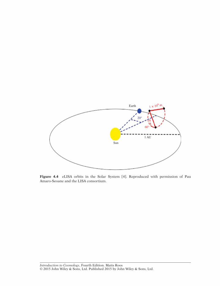
Earth
1 AU
Sun
1 × 10⁹ m
60°
20°
Figure 4.4 eLISA orbits in the Solar System [4]. Reproduced with permission of PauAmaro-Seoane and the LISA consortium.
Introduction to Cosmology, Fourth Edition. Matts Roos© 2015 John Wiley & Sons, Ltd. Published 2015 by John Wiley & Sons, Ltd.

0.175
0.15
0.125
0.1
0.075
0.05
0.025
0
0.05 0.025 –0.025
2001
2005
1992
2010
1995
2002
SgrA*
RA-offset (arcsec)
S2 (S02)
–0.05 –0.0750
Figure 5.6 Orbit of the star S2 moving around Sgr A* [10]. Copyright 2010 by the AmericanPhysical Society.

90°
6000
5000
4000
3000
Dℓ[μK
2 ]
2000
1000
02 10 50 500 1000
Multipole moment, ℓ
1500 2000 2500
18° 1° 0.2°
Angular scale
0.1° 0.07°
Figure 8.3 The best-fit power spectra of CMB temperature (T) fluctuations as a functionof angular scale (top x axis) and multipole moment (bottom x axis) [6]. Reproduced fromthe freely accessible Planck Legacy Archive with permission of Jan Tauber, European SpaceAgency.

500
DlT
E/l
[μK
2 ]
–0.4
–0.2
0.2
0.4 Planck 143 + 217
0
1000 1500 2000 2500
l
Figure 8.4 The temperature–E-polarization cross-power spectrum as a function of angularscale (top x axis) and multipole moment (bottom x axis) [6]. Reproduced from the freelyaccessible Planck Legacy Archive with permission of George Efstathiou, Kavli Institute forCosmology, University of Cambridge.

0.0 0.2 0.4 0.6 0.8 1.0
ΩM
0.0
0.2
0.4
0.6
0.8
1.0
1.2
1.4
Ωλ
Decelerating
Accelerating
No BigBang
Figure 8.5 The 1𝜎 and 2𝜎 cosmological constraints in𝛺m,𝛺𝜆 space using PanSTARRS1 super-nova data [13], Planck CMB data [6], BAO [14] and 𝐻0 data [6] with statistical and systematicerrors propagated. Reproduced with permission of Armin Rest for the PanSTARRS1 Collabo-ration.

0.0 0.1 0.2 0.3 0.4 0.5 0.6
ΩM
–2.0
–1.5
–1.0
–0.5
W
Figure 8.6 The 1𝜎 and 2𝜎 cosmological constraints in 𝛺m, 𝑊 space using PanSTARRS1supernova data [13], Planck CMB data [6], BAO [14] and 𝐻0 data [6] with statistical and sys-tematic errors propagated. Reproduced with permission of Armin Rest for the PanSTARRS1Collaboration.
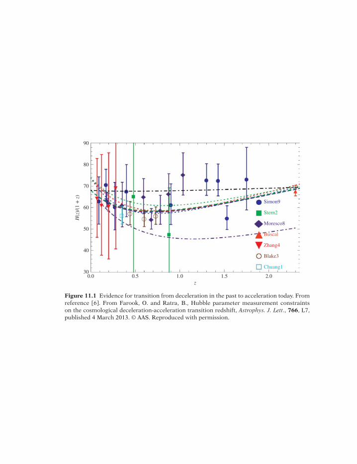
90
80
70
60
50
40
300.0 0.5 1.0
Simon9
Stern2
Moresco8
Buscal
Zhang4
Blake3
Chuang1
z
H(z
)/(1
+ z
)
1.5 2.0
Figure 11.1 Evidence for transition from deceleration in the past to acceleration today. Fromreference [6]. From Farook, O. and Ratra, B., Hubble parameter measurement constraintson the cosmological deceleration-acceleration transition redshift, Astrophys. J. Lett., 766, L7,published 4 March 2013. © AAS. Reproduced with permission.

0 0.5 1 1.5 2
Redshift z
–0.5
0
0.5
1
Δ (m
-M)
always accelerates
accelerates nowdecelerates in the past
always decelerates
flatopen
closed
Figure 12.1 Evidence for transition from deceleration in the past to acceleration today. Thedifference mM is defined in Equation (2.60). The blue line shows a model that fits the data,where acceleration happens at late epochs in the history of the universe (i.e. starting a fewbillion years ago, and billions of years after the Big Bang). The plot uses binned data from theUnion2 compilation [2]. With permission from the author.

WILEY END USER LICENSE AGREEMENTGo to www.wiley.com/go/eula to access Wiley’s ebook EULA.