SLAC-PUB-5149 December 1989

m

INTRODUCTION TO CONFORMAL

FIELD THEORY AND STRING THEORY*

Lance J. Dixon

Stanford Linear Accelerator Center

Stanford University

Stanford, CA 94309

ABSTRACT

I give an elementary introduction to conformal field theory and its applications to string theory.

I. INTRODUCTION:

These lectures are meant to provide a brief introduction to conformal field

-theory (CFT) and string theory for those with no prior exposure to the subjects.

There are many excellent reviews already available (or almost available), and most

of these go in to much more detail than I will be able to here. Those reviews con-

centrating on the CFT side of the subject include refs. 1,2,3,4; those emphasizing

string theory include refs. 5,6,7,8,9,10,11,12,13

I will start with a little pre-history of string theory to help motivate the sub-

ject. In the 1960’s it was noticed that certain properties of the hadronic spectrum

- squared masses for resonances that rose linearly with the angular momentum -

resembled the excitations of a massless, relativistic string.14 Such a string is char-

*Work supported in by the Department of Energy, contract DE-AC03-76SF00515. Lectures presented at the Theoretical Advanced Study Institute

In Elementary Particle Physics, Boulder, Colorado, June 4-30,1989

acterized by just one energy (or length) scale,* namely the square root of the string

tension T, which is the energy per unit length of a static, stretched string. For

strings to describe the strong interactions fi should be of order 1 GeV. Although

strings provided a qualitative understanding of much hadronic physics (and are still

useful today for describing hadronic spectra 15 and fragmentation16), some features

were hard to reconcile. In particular, string theory predicted an exactly massless,

spin-two particle that was nowhere to be found in the hadronic spectrum. 17

The current incarnation of string theory as a quantum theory of gravity

(and perhaps of all the fundamental interactions) came with the realization that

the massless, spin two particle should be identified as the graviton rather than as ._ _

some strongly interacting particle. l7 Since the characteristic energy scale of grav-

ity is the Planck scale, Mpl M 101’ GeV (N ew on’s t constant is GN = MF12), the

new identification necessitated resealing the string tension by some 38 orders of

magnitude! Other problems with string theory, such as the existence of a tachyon

(an unstable mode) and the absence of fermions, were cured by the introduction

of supersymmetry.18~1g~20~21 Th e explosion of interest in superstrings in 1984 fol-

lowed the observation that some superstring theories contain massless fermions

with parity-violating gauge interactions, like the known quarks and leptons. 22,23,24

Indeed, it was possible to identify a subset of the massless fermions and vector

bosons having the same gauge interactions as the quarks, leptons and gauge bosons

of the standard mode1.24 This opened up the possibility that superstring theory

might unify all the known interactions and thereby relate all observed masses and

coupling constants.

Obviously, this program has not yet been carried to completion. One of the

initial obstacles was that the original formulation of superstrings required space-

time to be ten-dimensional, not four-dimensional. Since then many ways have

been found to construct four-dimensional string theories, including ones whose low-

energy physics might be realistic.24>25j26j27 T h e constructions are generally termed

compactifications, because the first such constructions 28124 hid the extra six dimen-

sions by having them live on a compact manifold with a size of order the Planck

length. Later constructions have not required compact manifolds, and have led to

more varied possibilities for low-energy physics. However, each construction has

* I set ti = c = 1 everywhere

2

associated with it2g,30 a two-dimensional conformal field theory, which determines

the full particle spectrum and all the coupling constants. Conformal field theory

is therefore a necessary framework for understanding the types of physics that one

can expect from string theory.

String theory is not the only motivation for studying two-dimensional con-

formal field theory, however. The long-distance behavior of a statistical mechan-

ics system at a second-order phase transition (a critical point) is described by a

conformal field theory. 31y4 Also, many connections have recently been established

between conformal field theories and other exactly solvable (but not conformal)

two-dimensional field theories,32 as well as three-dimensional ‘topological’ field

th&iks.33~34 Here I will focus on the applications of conformal field theory to

string theory.

The organization of these lectures is as follows. In chapter II the propagation

of a free string is discussed via the Polyakov approach. In order to quantize the

string, various symmetries of the action must be gauge-fixed. This provides a

motivation for studying in chapter III some of the basic features of two-dimensional

conformal field theory, along with some simple examples. Most of this material can

also be found in ref. 3. In chapter IV the quantization of the bosonic string is carried

out and its mass spectrum is discussed. Chapter V describes briefly the superstring,

the heterotic string, and string interactions. Finally, chapter VI concludes with a

few comments on the prospects for superstrings.

II. FREE STRINGS AND CONFORMAL INVARIANCE:

A. Analogy to Point Particles

A massless, relativistic string is the one-dimensional generalization of a point

particle. String theory can therefore be developed in comparison to conventional

theories of point particles.

Recall that the quantum mechanics of interacting, relativistic particles can be

described in either a first- or second-quantized formalism. In a first-quantized for-

malism one first calculates the probabilities for free-particle propagation from point

x to point y. Then interactions are put in by hand: A certain amplitude (a coupling

constant) is assigned for one particle to emit another. These vertices allow all the

3

amplitudes in the theory to be built up, as Feynman diagrams that connect the

vertices together with free particle propagators. In a second-quantized approach,

by contrast, one defines field operators Ai that create and destroy particles, and

constructs a Lagrangian density in terms of those fields, L[Ai(z)]. When ,C is quan-

tized, its kinetic terms generate the propagators of the first-quantized approach,

and its interaction terms generate the vertices, so that all the first-quantized Feyn-

man diagrams are recovered. In addition, however, nonperturbative effects (such as

instantons) that cannot be represented by Feynman diagrams are revealed by the

second-quantized approach. Theories of point particles generally allow for many

possible kinds of interactions, and arbitrary values of coupling constants. This is

especially true if there are several different types of particles (fields) in the theory,

but even a theory of a single scalar field A can have arbitrary An couplings.

The first-quantized formalism for string theory proceeds similarly: One first

calculates amplitudes for free-string propagation, then assigns an amplitude (the

string coupling constant, 9,) for one string to emit another. In contrast to the par-

ticle case, where there may be several kinds of particles and many possible coupling

constants, in a given string theory there is only one kind of string and one coupling

constant g,, and only one ‘Feynman diagram’ at each order in gs.* In fact, string

interactions are uniquely determined, once the free-string propagation is specified!

Again, only perturbative amplitudes are easily accessible to this first-quantized

approach. The second-quantized approach to string theory is called string field

theory;35 it introduces string fields A(z(a)) th a create and destroy strings (a is a t

parameter along the string), and it (in some cases) generates ‘Feynman diagrams’

-that agree with the first-quantized results. In principle, string field theory also con-

tains nonperturbative information; in practice, no-one’has yet been able to extract

this information.

In these lectures only the first-quantized approach to string theory will be

discussed. I will begin by quantizing the motion of a free string by analogy to the

free-particle case, following ref. 5.

* For theories with open strings as well as closed strings, which will not be discussed in these lectures, there are a few ‘Feynman diagrams’ at a given order.

4

(4 (b) “74A1)

FIGURE 1

(a) A free particle propagating through space-time sweeps out a world-line. --- lb) A free string sweeps out a world-sheet.

B. Free Particle Action

A free point particle is characterized by its position in spacetime, Xp, where

CL = 0,1,2 ,..., D - 1 runs over the D space-time coordinates. As the particle

propagates in time it sweeps out a world-line described by Xp(r), where r is some

arbitrary parameter. See figure l(a).

The free-particle equation of motion (in flat space-time) is

d2Xc’ - - = 0,

dr2 which comes from varying the action

S(X) = m(length of world-line) = m J

ds

= -m/dr/z, (1)

where s is the proper time along the path.

The action (1) is difficult to quantize because of the square root. To avoid

the square root we introduce an auxiliary field g(r), which can be thought of as an

intrinsic metric on the world-line, and replace the action S(X) by

s(x,g) = ; /dT [& ($)2-m29(T)] * (2)

Eliminating g(r) from eq. (2) by its equations of motion leads back to the action

S(X) of eq. W, so the two actions are classically equivalent. The second form is

5

much easier to deal with quantum mechanically, however, because it is quadratic

in Xp. For example, the path integral JDDXp exp(-S(X,g)) is Gaussian in X

and can therefore be carried out exactly.

C. Free String Action and Symmetries

Rather than continuing with the particle example, let us now turn to the

string, which sweeps out a two-dimensional (2d) surface, the world-sheet, as it

moves through space-time. In these lectures I will discuss closed strings exclusively.

A closed string is a loop with no free ends, and so the world-sheet is a cylinder, as

shown in figure l(b). (If the string had been an open string, with two free ends,

the%&-ld-sheet would have been a strip.) A natural generalization of the particle

action (1) is the Nambu-Goto action 36

S(X) = -T( area of world-sheet) = -2’ J

dA

= -T drdg J

J-(&x)2(a,xy + (&X * 37X)2 ) (3)

where T is the string tension with dimensions of (length)-2. For applications to

hadronic physics, one would-set T N 1 GeV2 in eq. (3), whereas for applications to a

unified field theory incorporating quantum gravity one sets T N A$, N 1O38 GeV?

instead. As in the free particle case, the square root in eq. (3) can be avoided

by introducing an auxiliary field g,p( r,~), which is also the world-sheet metric.

Equation (3) can then be replaced by the classically equivalent action, 37

-

S(X,g) = -f d2a .J-s gffPa(yX’“~PXP, J

(4)

where g - det(g,p), a,@ = 0,l and (aO,ol) - (r,~).

Let us take the action (4) as the fundamental starting point for bosonic string

theory, and quantize it by considering a path integral

J

DDXp Dg,p e-s(xTg) .

over the auxiliary field g,p (the 2d metric) and over Xp. The g,p integral is an

integral over the intrinsic shapes of 2d surfaces, whereas the Xp integral is over

the different ways of embedding a 2d surface into D-dimensional space-time. The

boundary conditions on the path integral depend on the process being described.

6

To describe the propagation of a free, closed string, the 2d surface should be topo-

logically equivalent to a cylinder, as in figure l(b), and the boundary conditions on

the ends of the cylinder need to be specified. For many purposes it suffices to con-

sider the vacuum-to-vacuum amplitude, which is obtained by letting the cylinder

become infinitely long (.r E (- 00, oo)). The tension in the string forces the vacuum

state to have no spatial extent, so the ends of the cylinder are effectively collapsed

to points. Thus the 2d surface appearing in the free-string vacuum amplitude is

topologically a sphere.

Although we intend to discuss first the quantization of free strings, the path-

integral treatment of interactions is so similar that it bears mentioning here. In-

deed, -the path integral (5) 1 a so describes interacting strings with just a slight

change of boundary conditions. If one requires string interactions to be local, then

strings can only interact when they touch. Two strings that touch can join together

to become one, or in the time-reversed process a single string can split into two.

The vacuum amplitude will now have contributions in which the string splits and

rejoins many times. Each time it does so it creates a ‘handle’ on the 2d surface. All

of the surfaces are closed (they have no boundaries) like the sphere. The number of

handles on a surface is also called its genus and is denoted by h, h = 0, 1,2,. . . Two

surfaces are in the same topological class - i.e., they can be smoothly deformed

into each other - if and only if they have the same genus. We take the 2d metric

to have Euclidean signature (+, +), b ecause all surfaces with Minkowski signature

and genus h 2 1 are singular (the singularities occur wherever a time-like geodesic

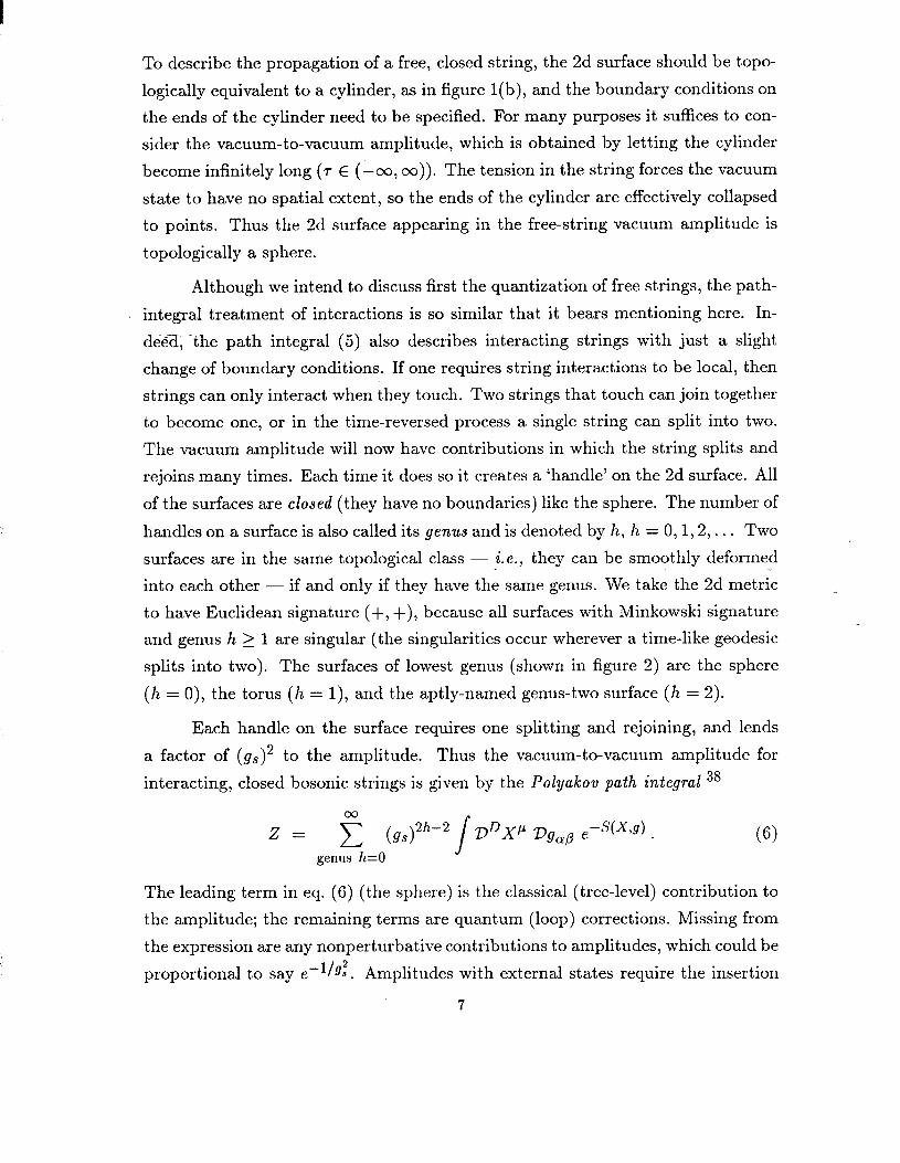
splits into two). The surfaces of lowest genus (shown in figure 2) are the sphere

(h = 0), the torus (h = l), and the aptly-named genus-two surface (h = 2).

Each handle on the surface requires one splitting and rejoining, and lends

a factor of (gs)2 to the amplitude. Thus the vacuum-to-vacuum amplitude for

interacting, closed bosonic strings is given by the Polyakov path integral 38

z = 5 (gs)2h-2 J DDXp Dgap eesCxJ) . genus h=O

The leading term in eq. (6) (the sphere) is th e c assical 1 (tree-level) contribution to

the amplitude; the remaining terms are quantum (loop) corrections. Missing from

the expression are any nonperturbative contributions to amplitudes, which could be

proportional to say e -l/g: . Amplitudes with external states require the insertion

7

(a) (W (cl

9 a.ro 65S111

FiGURE 2

Closed 2d surfaces of lowest genus: (a) the sphere, with genus h = 0, (b) the torus, with h = 1, (c) the genus-two surface.

of ‘vertex operators’ into (6) in order to create the proper boundary conditions on

the world-sheet; they will be discussed in section V.C.

The use of S(X, g) rather th an S(X) in (6) again greatly simplifies the path

integration over X p. The integral over gcrp can also be performed once we under-

stand the gauge invariances of S(X, g). The symmetries of S(X, g) are:

(1) Two-dimensional reparametrizations (general coordinate transformations),

(2) Local changes of scale (Weyl transformations),

9,&g + eX(u)9apt41

xqa> + xya>. (8)

(3) Global space-time PoincarC invariance,

9apw + 9apt”),

xqa> + fv~X”(U) + up. (9)

Equation (9) is a global symmetry and as such it is rather easy to deal with.

Equations (7) and (8) are local symmetries, however, and must be gauge-fixed in

order to quantize S(X,g).38

8

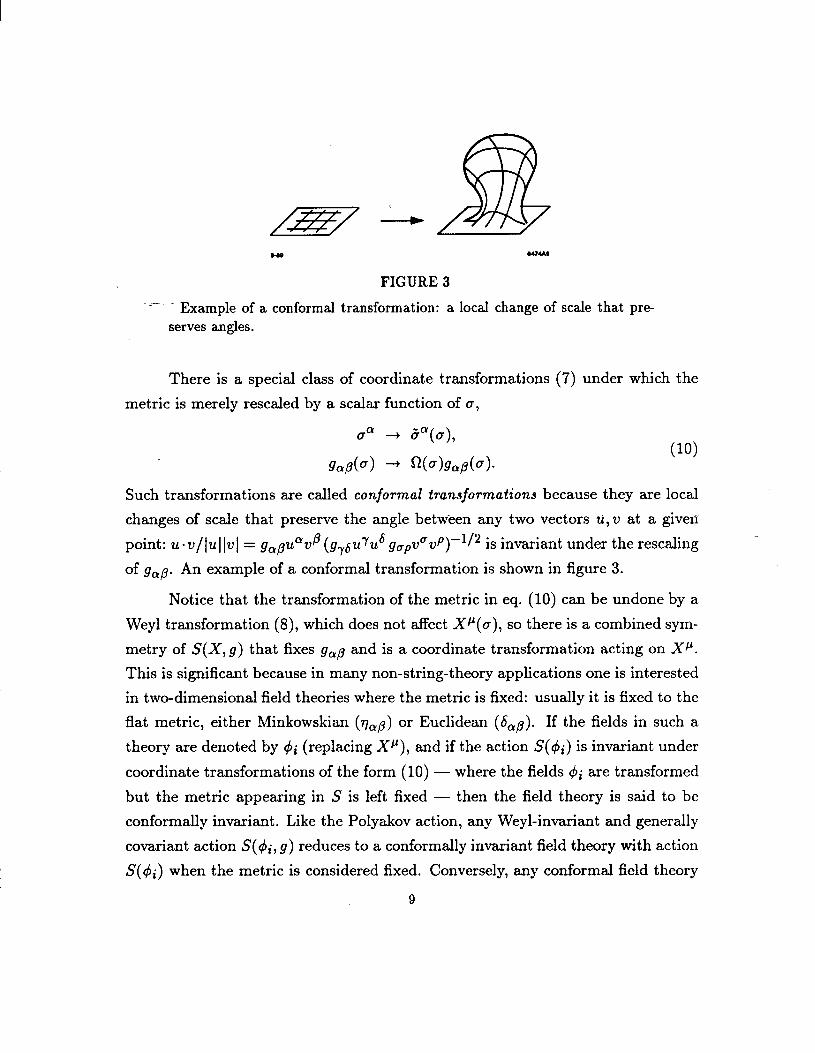
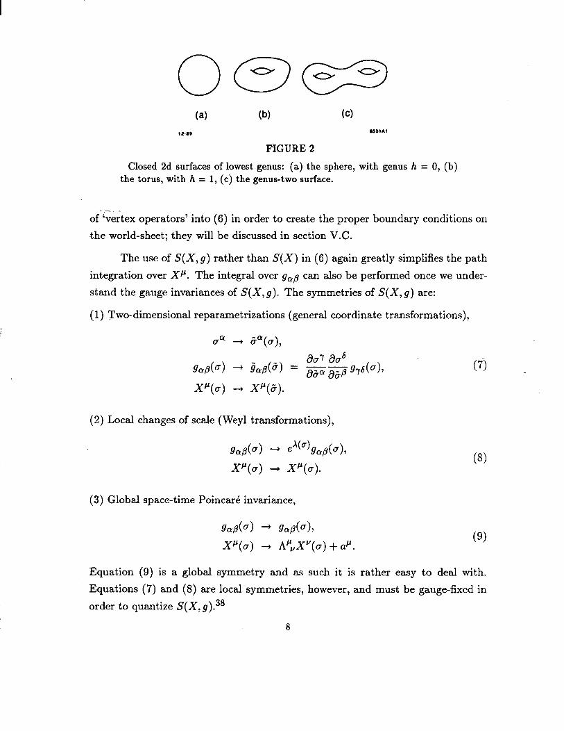
FIGURE 3

-- - Example of a conformal transformation: a local change of scale that pre- serves angles.

There is a special class of coordinate transformations (7) under which the

metric is merely resealed by a scalar function of U,

Such transformations are called conformal transformations because they are local

changes of scale that preserve the angle between any two vectors U, v at a given

point: u.v/~u~[v/ = gcrpuavP (gy6uru6 gUpvuvP)-1/2 is invariant under the resealing

of g,p. An example of a conformal transformation is shown in figure 3.

Notice that the transformation of the metric in eq. (10) can be undone by a

Weyl transformation (8), which does not affect Xp(a), so there is a combined sym-

metry of S(X, g) that fixes g,p and is a coordinate transformation acting on Xp.

This is significant because in many non-string-theory applications one is interested

in two-dimensional field theories where the metric is fixed: usually it is fixed to the

flat metric, either Minkowskian (qap) or Euclidean (6,~). If the fields in such a

theory are denoted by 4i ( re pl acing Xp), and if the action S($i) is invariant under

coordinate transformations of the form (10) - w h ere the fields 4; are transformed

but the metric appearing in S is left fixed - then the field theory is said to be

conformally invariant. Like the Polyakov action, any Weyl-invariant and generally

covariant action S(&, g) re d uces to a conformally invariant field theory with action

S(#i) when the metric is considered fixed. Conversely, any conformal field theory

9

gives rise to a Weyl-invariant theory when coupled to gravity. Conformal field

theories play an important role in string theory because one can replace portions

of the Polyakov action S(X,g) by the action S(&, g) for some other conformal

field theory coupled to the 2d metric. The (phenomenological) reason for making

this replacement is that, as will be seen in chapter IV, the Polyakov action only

has a simple quantization if there are 26 space-time coordinates Xp, which is 22

more than the four we observe. If the terms in the Polyakov action containing

the 22 unwanted coordinates are replaced by an appropriate action S($;, g), in a

procedure known as compactification, then four-dimensional (super)string theories

can be constructed. With this application in mind, I will now make a rather long

digression to discuss the general properties of 2d conformal field theories. In chap-

ter IV I will return to the problem of quantizing both the Polyakov action and its

compactified counterparts (and the supersymmetric versions of these).

III. TWO-DIMENSIONAL CONFORMAL FIELD THEORY:

A. The Energy-Momentum Tensor and Primary Fields

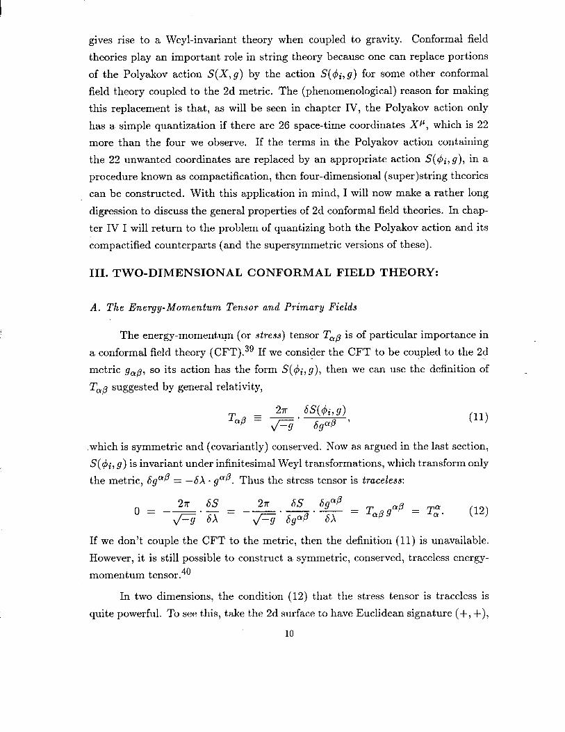
The energy-momentum (or stress) tensor Twp is of particular importance in

a conformal field theory (CFT). 3g If we consider the CFT to be coupled to the 2d

metric g,p, so its action has the form S(&,g), then we can use the definition of

Tap suggested by general relativity,

-which is symmetric and (covariantly) conserved. Now as argued in the last section,

S($i, g) is invariant under infinitesimal Weyl transformations, which transform only

the metric, SgLyp = -6X - g 4 Thus the stress tensor is traceless: .

If we don’t couple the CFT to the metric, then the definition (11) is unavailable.

However, it is still possible to construct a symmetric, conserved, traceless energy-

momentum tensor.40

In two dimensions, the condition (12) that the stress tensor is traceless is

quite powerful. To see this, take the 2d surface to have Euclidean signature (+, +),

10

and introduce complex coordinates, z and z?. The Polyakov path integral (6) re-

ceives contributions from surfaces of arbitrary genus; here I will concentrate mostly

on the genus h = 0 term (the sphere), and later a little on the h = 1 term (the

torus). If the surface has the topology of a sphere, it turns out that z and z can

always be chosen so that the volume element has the form d2a = e’(“p’)dz do. A

Weyl transformation can then be used to set e’ E 1, so that d2a = dz &. Thus

the theory is effectively being considered on the complex z-plane. (The curvature

of the sphere has been pushed off to z = 00 in this description.) Alternatively,

the theory might have been initially formulated on the plane with a flat metric,

as would usually be the case in the statistical mechanics context. In any case, the

components of the metric are

9,z = : 7 9z.z = gz = 0. (13) Now all tensor fields $ei:::&, carry Z,Z indices, which can be lowered using the

metric (13), to obtain $z...z~...T as the most general form.

In particular, the components of the stress tensor Top are

T., = a(Trr - Tua - 2iTru), TE = i(T,, - Tua + 2iTru), T,F = i(T,r + Tw).

(14) Weyl-invariance then implies via eq. (12) that Tzy = 0. Combining this with

conservation of the stress tensor, 8”Ta~ = 0, or in complex coordinates

WY,, +&T’-;, = &Tzz + &TZF = o, (15)

one sees that the two remaining components of the stress tensor are a holomorphic

-component T,,(z) 3 T( ) z an an antiholomorphic component TV E F(Z). This d

feature allows one to say a great deal about the behavior of the stress tensor in

any 2d CFT.

In two dimensions there are an infinite number of conformal transformations

of the form (10). (Th ere are only a finite number in more than two dimensions.)

In fact, any analytic transformation of the complex coordinates,

z + z’= f(z), z + &f(F), (16)

is a conformal transformation, leaving gzz = 9z-z = 0 and resealing gzs by Idz/dz’12.

An arbitrary tensor field dz...zf...z with n of the z indices and E of the z indices

11

transforms under (16) as

4) *...rF...ZW) + 4%...rH...F (4 = (-$)” ( $b...~i...dz.‘). (17) Here the exponents h = n + A, h = z + A allow for the possibility of a scaling

dimension A for $ in addition to its fixed Lorentz properties. (In two dimensions

the properties of a field under the Lorentz group, SO(1, 1) or SO(2) = U(l), are

characterized entirely by the field’s ‘spin’ n -?i = h -h.) In fact, equation (17) only

states how a classical tensor field transforms. At the quantum level, 4 is promoted

to an operator, and if it is a composite field there may be issues of operator ordering,

etc. which may spoil eq. (17), as will be seen in a while. Nevertheless some fields

L-called primary fields - will retain this transformation law and will play an

important role in the CFT.

B. Radial Quantization and Conserved Charges

Now consider the components of the stress tensor T(z) and F;(Z) as operators

in a quantized CFT. If the space direction is considered periodic, i.e. it is a circle,

then space-time is a (Euclidean) cylinder, which can be parameterized by 5 = r+ig,

T = 7- - ia. Instead of quantizing the conformal field theory on the cylinder, it

proves convenient to conformally map the cylinder to the complex plane, defining

the coordinates of the plane to be

* = ,c = ,r+ia , 7 = ,T = ,-ifl* (1%

The distant past (r = -oo) is mapped to the origin z = 0, and the distant future

(7 = +oo) to 121 = ccl. The r or ‘time’ direction now points radially outward

-from the origin. We continue to treat this direction as the quantization direction,

however. In particular, correlation functions in this radial quantization scheme3g

are defined via radially-ordered products of fields, namely

Wlh,%) 42(z232)) = {

4l(zl,a 42(22,22) if 1211 > 1221,

~2(~2,~2Mh~l) if 1221 > 14 (20)

The importance of T(z) and T(Y) is as the generators of infinitesimal con-

formal transformations. Every continuous symmetry of a field theory has associ-

ated with it a conserved current, P(a) with &J” = 0. The conserved charge

12

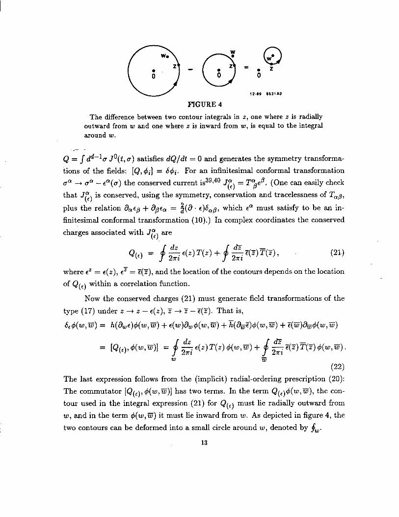
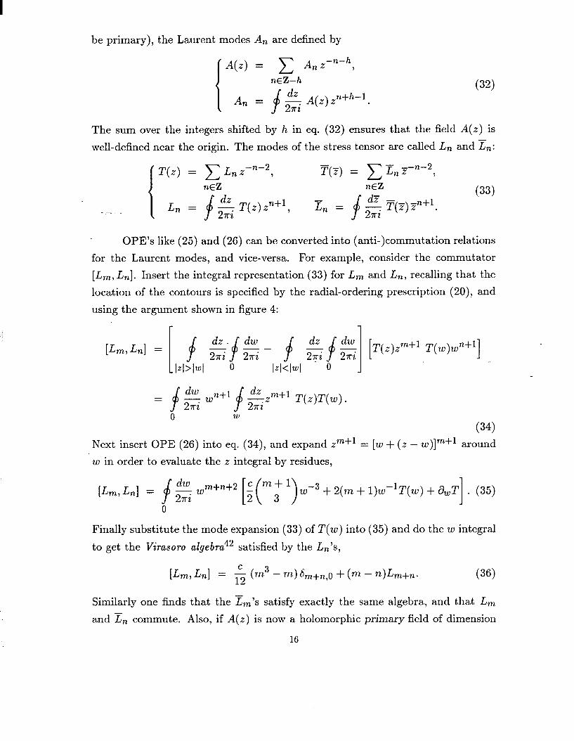
(TJ- @jfy F’IGURE 4

The difference between two contour integrals in I, one where t is radially outward from w and one where z is inward from w, is equal to the integral around w.

._ _ Q = j-dd-’ CJ J’(t, a) satisfies dQ/dt = 0 and generates the symmetry transforma-

tions of the fields: [&,&I = S$i. F or an infinitesimal conformal transformation

tla + QQ - P(a) the conserved current is 3g,40 Jc, = TUpeP. (One can easily check

that Jc, is conserved, using the symmetry, conservation and tracelessness of Tap,

plus the relation &E, + 8~6, = $(a. e)b,p, which P must satisfy to be an in-

finitesimal conformal transformation (lo).) I n complex coordinates the conserved

charges associated with Jc) are

Q (0 = f &E(Z) T(z) +- f 2 z(z) T(z), (21)

where ef = E(Z), E’ = U(Z), and the location of the contours depends on the location

of Q(c) within a correlation function.

Now the conserved charges (21) must generate field transformations of the

type (17) under z + z - E(Z), Z -t Y - Z(Z). That is,

S~~(W,EJ) = h(&&(w,~) + +~)&,g+u,~) + ~(~+@J,~) + @)&@JJ)

(22) The last expression follows from the (implicit) radial-ordering prescription (20):

The commutator [Q(,),~(w,E)] has two terms. In the term Q(,)~(w,w), the con-

tour used in the integral expression (21) for Q(E) must lie radially outward from

20, and in the term +(w,F) it must lie inward from 20. As depicted in figure 4, the

two contours can be deformed into a small circle around W, denoted by jw.

13

C. Operator Product Expansions and Commutation Relations

Equation (22) determines the short distance behavior of T(z) and T(Y) near

c$(w,w). The short distance behavior of operators is usually described by an oper-

ator product expansion 41 (OPE),

4i(4 $j(Y> - CCijk(x - Y) 4k(Y) as x + Ye (23) k

The functions cQk(z - y) are called operator product coefficients; their spatial de-

pendence is determined by the Lorentz and scaling properties of the fields $i, #j, r$k.

In two dimensions they are all proportional to (z - w)“(z - w)P for some cy, ,B de-

pending on ;,j, Ic. In particular, the OPE of T(z) with any field $ is constrained by

the requirements of single-valuedness (as z moves around W) and y-independence

to have the form

T(z)$(w,w) = c(z - ZU)~ O&U,W). (24) nEZ

Substitution of the expansion (24) into (22) leads to

A field 4 that has an OPE with the stress tensor of the form (25) - or equivalently,

that transforms like eqs. (17), (22) under conformal transformations - is called

.a primary field or conformal field, and (h, ?I) are called its conformal or scaling

dimensions.3g

As remarked above, fields which transform like eq. (17) at the classical level

may fail to do so at the quantum level. The prime example of this phenomenon

is the stress tensor itself: T(z) has (h,h) = (2,0), but its OPE with itself has an

additional term:3g

T(z) T(w) N (z $4 + 2T(w) + = (z _ w)2 * - w + finite* (26)

Equation (26) is the most general form of the OPE consistent with the holomor-

phicity of T( ) z and its role as the generator of conformal transformations. Here c

14

is a real number, called the central charge, which depends on the conformal field

theory and is nonzero in any nontrivial theory. Later in this chapter c will be

calculated for some simple CFTs. There is an analogous OPE of T(z) with itself,

T(F)T@) N 42 2qq if@ (F - $4 + (F _ ,J2 + ~--w + finite. (27)

In section 1I.C it was mentioned that any CFT, when coupled to the 2d

metric, gives rise to a Weyl-invariant theory. Actually this is not quite true, due

to the presence of the central charge c. Notice that*

W&>Tww(~) = + &aw [ 2 (E) +...I = c-~a~~wd2~(z-w)+ . ..)

(28)

where the identity

+&lnIZ-W12 = * -J-- = ( >

7rd2)(z - w) Z-W

(29)

has been used. Taking k of eq. (28) and then using conservation of Tap (15) to

replace Tzz, Tww by TZy, T,z, one gets

T&) Twz(w) = c . ; &&&2)(z - w). (30’)

On the other hand, T,y is related via eq. (12) to the variation of the action -

or at the quantum level, the effective action - under a Weyl transformation (8):

TZF N SS,ff/GX. If we write g,p(g) = eX(“)i,p(a), where i,p is some reference

-metric and X is the conformal factor, then equation (30) means that the quantum

path integral 2 for the CFT depends on the conformal factor, according to

d2a &Max . 1 This formula will be needed when we return to the quantization of the Polyakov

action in chapter IV.

An important feature of holomorphic fields like Tzz(z) is that they can be

Laurent expanded. Given a holomorphic field A(z) with dimension h (A need not

* I follow the discussion of ref. 7 here.

15

be primary), the Laurent modes A, are defined by

J A(Z) = C Anzmnph, nEZ-h

\ An = f 2 A(.z)z~+~-‘. (32)

The sum over the integers shifted by h in eq. (32) ensures that the field A(z) is

well-defined near the origin. The modes of the stress tensor are called Ln and Ln:

T(Z) = C Lnzens2, F(F) = C EnZBns2, nEZ nEZ

Ln = ._ _ f

2 T(z) zn+‘, (33)

En = f

2 T(F) zn+l.

OPE’s like (25) and (26) can be converted into (anti-)commutation relations

for the Laurent modes, and vice-versa. For example, consider the commutator

[Lm, Ln]. Insert the integral representation (33) for L, and Ln, recalling that the

location of the contours is specified by the radial-ordering prescription (20), and

using the argument shown in figure 4:

= fg um+l~~~~+~ T(z)T(w).

0 W

(34)

Next insert OPE (26) into eq. (34), and expand z?+’ = [w + (z - w)]“+’ around

w in order to evaluate the z integral by residues,

[Lm,Lnl = f 2 wm+n+2 [K (VI 3’ ‘) wF3 + ~(772 + ~)w-~T(w) + awn] . (35) 0

Finally substitute the mode expansion (33) of T(w) into (35) and do the w integral

to get the Virusoro algeara42 satisfied by the Ln’s,

[Ln7Ln] = s (m3 - m> &n+n,O + Cm - n)bn+n- (36)

Similarly one finds that the Em’s satisfy exactly the same algebra, and that L,

and Ln commute. Also, if A( ) z is now a holomorphic primary field of dimension

16

h, equations (25), (32) and (33) combine to give

[Lm, An] = ((h - l)m - n)Am+n. (37)

D. Primary and Descendant States

Using equation (21), one can see that the conformal transformations gener-

ated by Ln and En are z + z - en2 n-t’) where en is a complex constant. Thus L-1,

1-1 generate uniform translations of the complex plane, z + z - e-1, and Lo, Lo

generate dilatations and rotations, z t (1 - eo)z. Since the radial direction is the

‘time’ direction, dilatations are time translations, and Lo + Lo plays the role of

thk%amiltonian. The energies of states are given by their Lo, Lo eigenvalues. ‘In

states’ 14) are created by fields acting in the distant past, at z = 0: I$) = d(O) IO).

Similarly, (41 - (01 d(co). If ~(z,z?) is a primary field, then 14) is said to be a

primary state. Primary states are annihilated by the Ln modes with positive n:

Ln I$> = f

n+lT(z)d(0) IO) =

f ’

2 zn+’ z-2h4(0) +Z’%(O)] 10)

0

0 = if n 2.1, hlq5) if n = 0.

(381

Note from eq. (36) that [Lo, Ln] = -nLn, SO the operator Ln lowers the

eigenvalue of Lo by n units. (The same is also true of the more general operator

An, as seen from eq. (37).) Th us a tower of descendant states above any primary

state 14) is built up by acting with the Lo-raising operators L-n (n > 0) to get

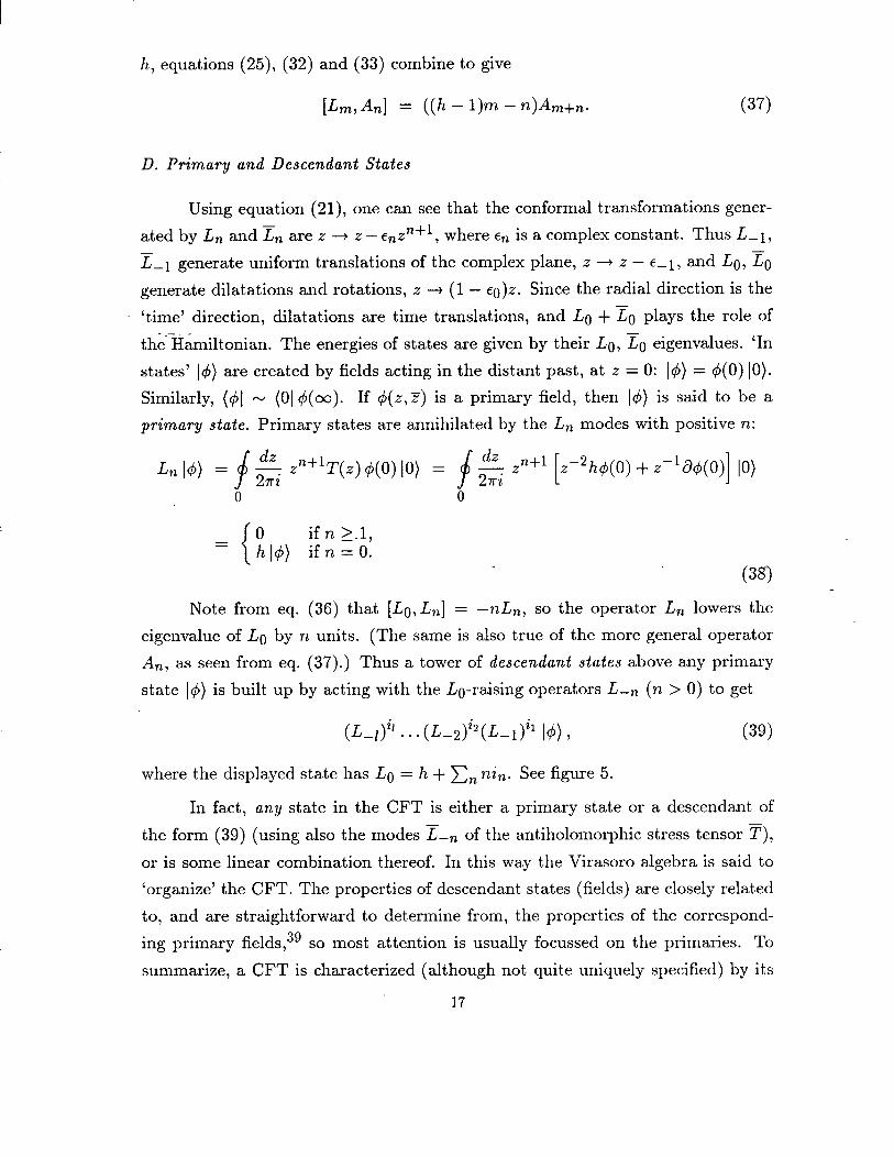
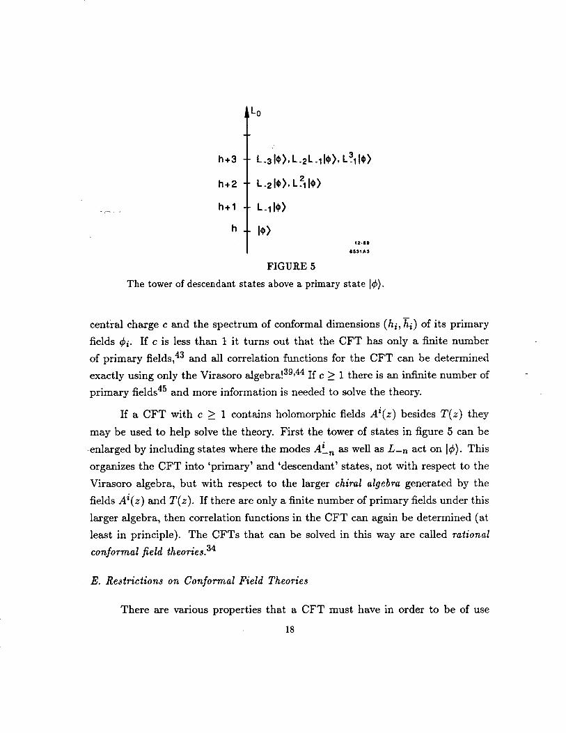
(L-/)i’ . . * (L-2P(L-lP 14, (39) where the displayed state has Lo = h + En nin. See figure 5.

In fact, any state in the CFT is either a primary state or a descendant of

the form (39) ( using also the modes L-n of the antiholomorphic stress tensor T),

or is some linear combination thereof. In this way the Virasoro algebra is said to

‘organize’ the CFT. The properties of descendant states (fields) are closely related

to, and are straightforward to determine from, the properties of the correspond-

ing primary fields,3g so most attention is usually focussed on the primaries. To

summarize, a CFT is characterized (although not quite uniquely specified) by its

17

h+3 L-&‘)~L-2L.lk’)~ Lf,bt’)

h+2

h+l L-1 I40 h I40

12-20

2521A.Y

FIGURE 5

The tower of descendant states above a primary state 14).

central charge c and the spectrum of conformal dimensions (hi,&) of its primary

fields +i. If c is less than 1 it turns out that the CFT has only a finite number

of primary fields,43 and all correlation functions for the CFT can be determined

exactly using only the Virasoro algebra. 13g~44 If c > 1 there is an infinite number of - -

primary fields45 and more information is needed to solve the theory.

If a CFT with c 2 1 contains holomorphic fields A”(z) besides T(z) they

may be used to help solve the theory. First the tower of states in figure 5 can be

-enlarged by including states where the modes Ai, as well as L-, act on 14). This

organizes the CFT into ‘primary’ and ‘descendant’ states, not with respect to the

Virasoro algebra, but with respect to the larger chirul algebra generated by the

fields Ai and T(z). If th ere are only a finite number of primary fields under this

larger algebra, then correlation functions in the CFT can again be determined (at

least in principle). The CFTs that can be solved in this way are called rational

conformal field theories. 34

E. Restrictions on Conformal Field Theories

There are various properties that a CFT must have in order to be of use

18

in string theory. (Some of the properties are required by other CFT applications

too.) I will describe three of the most important ones here.

(1) Unitarity. All states in the 2d CFT Hilbert space should have non-

negative norm. In string theory, negative norm states in the 2d Hilbert space lead

to negative norms for particle states in space-time. Unless the negative norm states

decouple from scattering amplitudes of physical particles, it is impossible to have a

unitary time evolution, as is required by quantum mechanics. Some negative-norm

states are automatically decoupled in string theory, namely the time-like polar-

ization states of vector and tensor particles, etc., as will be seen in section 1V.C.

On the other hand, the CFTs that describe string ‘compactifications’ (see sections

1V:B and 1V.C) h ave to be unitary, because no mechanism exists for decoupling

any negative norm states that they might contain. 30

To check unitarity in a CFT, one has to calculate norms, which requires

knowing how Hermitian conjugation acts on operators. The action is easiest to

determine in Minkowski space, that is by mapping the z-plane back to the cylinder,

and then Wick-rotating so that it becomes Minkowskian. One finds that the modes

A, of any real, holomorphic field A(z) satisfy AL = A-,. In particular, the

Virasoro modes satisfy Lk = L-,. Using this information it is possible to show,43

for example, that there is only a discrete set of unitary CFTs with, central charge

c < 1, which have

and a finite number of primary fields for each m, with conformal dimensions

hd4 = ((m + 1)~ - mq)2 - 1

4m(m+l) ’ l<p<m-I, l<q<p. (41)

The restrictions imposed by unitarity alone on CFTs with central charge c > 1 are

very weak; however, unitarity in combination with other constraints can be useful.

(2) S in e v ue correlation functions. The quantity gl - af d

(4lh~l) * * * hzG%% )) should be well-defined on the complex plane, which means

that it should not change when any point zi is carried continuously around any

other point zj.

(3) Modular invariance. The Polyakov path integral (6), when generalized

to include external states, requires correlation functions to be well-defined on any

19

closed 2d surface, and different parametrizations of the same 2d surface should

give the same answer. An important feature of surfaces with genus h 2 1 is a set

of complex parameters, or mod&, 46 which are global obstructions to the choice

of coordinates that we made on the sphere (h = 0), namely z, F with d2a =

eX(Z~Ti)dz&. Surfaces with h > 2 have 3h - 3 complex moduli, denoted by ri, - i = 1,2,..., 3h - 3. The torus (h = 1) h as one complex modulus, denoted by r

(which should not be confused with the world-sheet time parameter r used earlier).

For each surface with h > 1 there are ‘large’ reparametrizations, called modular

transformations, which are not continuously connected to the identity, and which

change the values of the moduli, but which do not change the shape of the surface.

Any correlation function on the surface should therefore be invariant under modular

transformations.

The simplest modular transformations are those of the torus. Also, modu-

lar invariance of the vacuum amplitude on the torus (usually called the partition

function) is one of the strongest constraints on a CFT.45j47p25 A two-dimensional

torus can be constructed by identifying points on the complex z-plane that differ

by vectors of a 2d lattice. It is conventional to set the second of the two basis

vectors of the lattice to 1 by a scale transformation. Then the identification of

points is

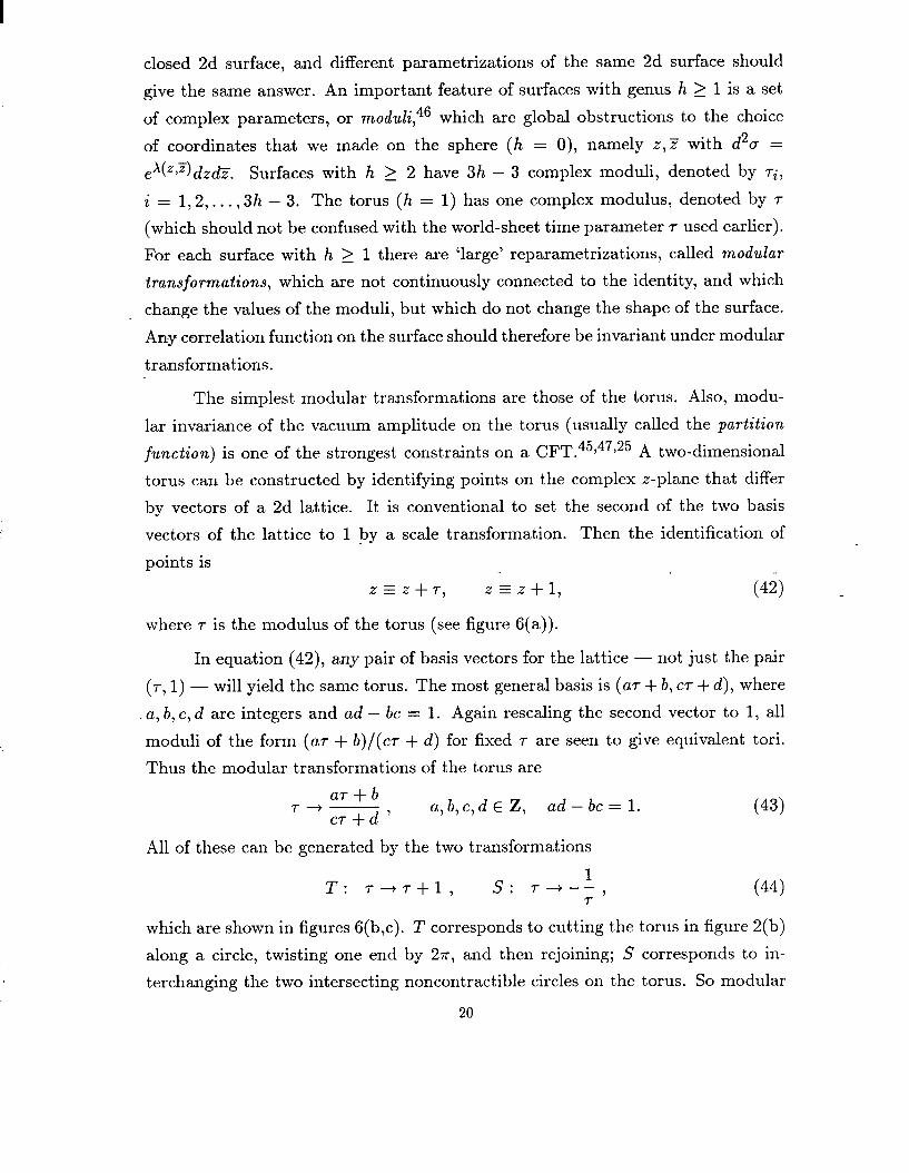
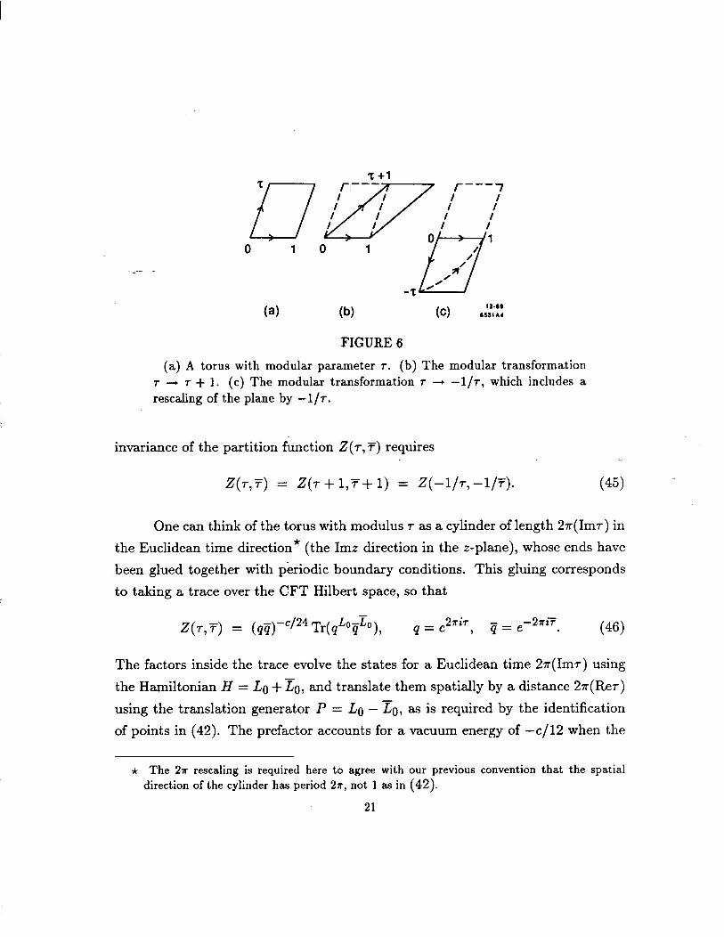
2=,Z+7, 2=2+1, (42) -

where r is the modulus of the torus (see figure 6(a)).

In equation (42), any pair of basis vectors for the lattice - not just the pair

(r, 1) - will yield the same torus. The most general basis is (ur + b, cr + d), where

a, b, c, d are integers and ad - bc = 1. Again resealing the second vector to 1, all

moduli of the form (ur + b)/(cr + d) for fixed r are seen to give equivalent tori.

Thus the modular transformations of the torus are

(43) All of these can be generated by the two transformations

1 T: T-+7+1, s: T+---, (44) 7

which are shown in figures 6(b,c). T corresponds to cutting the torus in figure 2(b)

along a circle, twisting one end by 27r, and then rejoining; S corresponds to in-

terchanging the two intersecting noncontractible circles on the torus. So modular

20

(4 (W

FIGURE6

(a) A torus with modular parameter T. (b) The modular transformation r -+ T + 1. (c) The modular transformation 7 -+ -l/~, which includes a resealing of the plane by -l/7.

invariance of the partition function .Z(r, Y) requires

Z(T,T) = z-(7- + 1,7+ 1) = 2(-l/r, -l/7). (45) -

One can think of the torus with modulus r as a cylinder of length 27r(Imr) in

the Euclidean time direction* (the Imz direction in the z-plane), whose ends have

-been glued together with periodic boundary conditions. This gluing corresponds

to taking a trace over the CFT Hilbert space, so that

Z(r,7) = (qij)-c/24 Tr(qL”$O), (46)

The factors inside the trace evolve the states for a Euclidean time 2x(Imr) using

the Hamiltonian H = Lo +&, and translate them spatially by a distance 2r(Rer)

using the translation generator P = Lo - &, as is required by the identification

of points in (42). The prefactor accounts for a vacuum energy of -c/12 when the

* The 2?r resealing is required here to agree with our previous convention that the spatial direction of the cylinder has period 27, not 1 as in (42).

21

torus is constructed as in (42). Th e condition that the expression (46) for Z( r, 7)

is invariant under T is easy to impose:

z(~ + 1,~ + 1) = (qq)-c/24 Tr(qLOqLO e2?ri(LfJ-r--O)), (47)

so the requirement is that Lo -Lo must be an integer for every state in the theory.

The S invariance condition is less trivial; we will see in the next few sections how

it is satisfied by partition functions for some simple CFTs.

F. Massless Free Boson Example

___ _Now that I have described some of the general properties of 2d CFTs, I turn

to a few simple examples, which are just free field theories. Even though they are

rather trivial as 2d field theories, they nevertheless have nontrivial string theory

applications.

First consider a massless free boson X, with the action

S(X) = $ d2a &Xa”X. J

(48)

This action is precisely the Polyakov action (4), with the 2d metric fixed to be flat,

and with X interpreted as a single space-time-coordinate. The propagator for X is

obtained as usual by inverting the kinetic term, so it satisfies &Y(X(~)X(~‘)) =

-47rsqa - o’), or B&(X(z,Z)X( w,w)) = -TS(~)(Z - ZU), which is solved by

-

(X(z,Z)X(w,W)) = -In Iz - ~1~. (49)

-From the propagator (49) one can also read off

(&X&J> = -( Z

ywj2 ,

w%w = -@ 1,j2 7 (50)

(&X&X) = 7rd2)(z - 20).

The vacuum expectation values (50) 1 a so g ive the singular terms in the corre-

sponding OPEs. The reason is that the products on the left-hand side of OPEs are

implicitly ‘time’-ordered (radially-ordered), whereas the composite operators ap-

pearing on the right-hand side of such OPEs are generally normal-ordered. Wick’s

22

theorem states that the difference between the two kinds of products is obtained

by Wick contractions, which for &X&X, etc., is just the corresponding vacuum

expectation value. For example,

&X&X = (z _‘,)2 + : &X&X :

N (z Iy)2 + : &X&X : + O(z - to). (51)

As usual, (51) can be converted to commutation relations for the modes on of L&X,

which are defined by

(52) ._ _

They obey [am, on] = mS,+,,o. Similarly the modes Zn of %X obey [Em, ZCn] =

m6rn+n,07 and [cY~, Z!~] = 0. These are just the commutation relations of an infinite

set of harmonic oscillator creation and annihilation operators, a, = t-1 fia-n, an =

To show that the massless free boson theory actually is conformally invariant,

it suffices to show that the component !I’,,, of the stress tensor is holomorphic and

has the OPE (26). T,, can be obtained either by the Noether procedure or by the

definition Z’,, - SS/Sgzz. One finds (after removing the factor of & which appears

explicitly in eq. (21) and defining the composite operator via normal-ordering) the

free boson stress tensor

T** = T(z) = -; : &X&X : . (53)

-First let’s check the OPE of T( ) z with 8,X, using (two) Wick contractions to

obtain the singular terms:

T(z)&X = -; : &X&X : 8,X N -f .2.

. (54)

Equation (54) verifies (cf. eq. (25)) that &X is a primary field of dimension

h = 1. The OPE of ?? with &X is finite (up to delta functions), so h = 0. These

are precisely the dimensions of the classical tensor field 8,X, so the free field has

acquired no anomalous dimension.

23

The OPE of T with itself is computed similarly. There are two ways to do

the double Wick contractions for the most singular term, and four ways to do a

single contraction:

T(z) T(w) = ; : &X&X : : &,X&X : N i.2

(z-w)4

112 - (z - w)4 +

2( - $a,X&X) (z - w)2

+ a,(+wxa,x) +*-*,

z-w (55)

which shows that the massless free boson is a CFT, with central charge c = 1 (cf.

eq. (26)). Note that the Polyakov action with D space-time dimensions contains ._ _ D free bosons, Xp, p = 0, 1, . . . , D - 1, and that such a system has central charge

-c = D.

Besides dXp and ??Xp, there is another important set of primary fields that

one can build out of D free bosons, namely the normal-ordered exponentials

Vk(z,Z) = : exp(iL.X(z,Z)) : . (56)

One can easily use Wick contractions to derive the OPE

a,xp eik.X(w,W) N -ikpe eik.X(w,W) + . . . , z-w

and from it

2 eik.X(w,z) + . . .

(57) -

(58)

(and an analogous OPE with ?T), so that the conformal dimensions of vk are h =

ii = k2/2.

Acting on the vacuum state IO), vk creates a state Ik) s eikei IO), with

‘momentum’ k. Here ? is the zero-mode of X, which is canonically conjugate to

the ‘momentum’ I; - oo = ~0: [?,$I = i. ‘Momentum’ here is not 2d momentum

(we always work in position space in 2d), but rather a global internal symmetry

of the 2d CFT, which in string theory is interpreted as space-time momentum.

The states Ik), like the vacuum IO), are annihilated by all of the positive frequency

modes (annihilation operators) om, En. The complete free boson Hilbert space is

24

obtained by acting on the states I k) with all the negative frequency modes (creation

operators); it consists of all states of the form

(cL#’ . . . (cL~)~~(E’-~)~~ . . . (a-l)31 Ik) , k E R. (59)

One can check that the free boson theory is unitary by showing explicitly that every

state in the Hilbert space has positive norm, using the Hermitian conjugation rules

AC: = Oi-n, 5; = E-n, the oscillator commutation relations, and the norm (ICI k) = 1

for the momentum states.

With the full Hilbert space (59) one can also compute the partition function

Z(r,7) and verify that it is modular invariant. It is easy to see that the trace (46) ._ _

is a product of independent contributions from the different oscillators o-n and

the ‘momentum’ k. The contribution of the states {(o-n)i IO), i = 0,1,2,. . .},

with Lo = in, is

00

c

1 Q

in = 1 +qn +qzn + . . . = - i=O

l-qn’ (60)

The-contribution of the continuum of states Ik), with Lo = k2/2, is

00 00 J fJk (43 - k2/2 -

J & ,-2r Imr k2 - (2 Imr)-1/2. _

(61) -00 -CO

Putting all the factors together, the free boson partition function is

2(~,7) = (2 Imr)-112 q-1/24 fi (1 - qn)-l

2

= (21mr)-1/21~(r)l-2, (62) n=l

where v(r) E q1/24 nrzl(l - q”) is the Dedekind eta function. The modular

transformation properties of the eta function are well known5

r&T + 1) = P/12Tj(T) ) q(-l/-r) = (-iT)1/2q(7) .

Using also Im(-l/r) = (3-Y)-l1 mr, we see that Z( r, 7) is indeed modular invariant.

G. Free Boson on a Circle

The free boson CFT can be modified slightly by changing the boundary

conditions on X. Before it was assumed that the field X could take on any real

25

value. Now let us take the values of X to lie on a circle of radius R. That is, we

identify

X G X + 27rR. (63)

This identification has two consequences. First, the ‘momenta’ k are quantized,

because the operator exp(ifi . 27rR) that translates states by 27rR must now be

trivial, i.e., equal to 1. Thus for any k, exp(ik . 27rR) = 1, or k = m/R for

some integer m. Second, there are new ‘winding’ states in the theory, because the

boundary conditions

X(a + 27r) = X(a) + 27rR. n, nEZ (64) ._ _

are allowed by the identification (63).

To describe the new states we define left-moving and right-moving compo-

nents of X(z,Z),

X(&Z) = X,(z) +X,(z), (65)

with OPEs

XL(Z) XL(W) N -ln(z - w), X,(Z) XR@> - - In(Z - Zo), (66)

and mode expansions

X,(z) = in - ilj,lnz + i c 1 - O!nZmn,

n#O n

X,(S) = ?R - ijR In Z + i C k ZnYZen.

n#O

(67)

For momentum k = m/R and winding number n in (64) the eigenvalues of the

zero-modes (fin, fiR) are

tb IcR) = m,nE Z.

None of the nonzero modes on, Zn are affected by the change in boundary condi-

tions on X, so the Hilbert space (59) is unaltered except for the replacement of Ik)

by IkL, kR), with (kL, kR) given by (68).

The field XL(Z) h as a multi-valued OPE (66) with itself. However, X,(z)

does not appear by itself in the CFT of a free boson on a circle, and the fields that

26

do appear are cleverly arranged to have single-valued OPEs and hence single-valued

correlation functions. Let us check that the primary fields ei(k~X~-tkRXR) making

the states IkL, kR) h ave single-valued OPEs. Using the Wick contractions (66)

repeatedly, one can show that

ei(kdL+kRXR) (z,~) ,i(k;XL+kkxd(w E)

- (z-w) kL.kL(, _ qk& ei((k~+k:)Xr.+(kR+kk)Xx)o,~) + . . . . (69)

If z is carried around w, so that z - w --t (z - w)e2*i, z - w + (Z - ,)e-2ni,

then the OPE (69) d evelops a phase exp 2ri(kL . kk - kR. kb), which for arbitrary

(kL, kR) and (ki, kk) is not equal to 1. But the values of kL, kR should be taken

from the set (68), in which case the phase is

exp2;rri [(g + 9) (g + q) - (I;t - 9) ($ - q)]

= exp 2ri(mn’ + m’n) = 1,

(70)

so the OPE is single-valued.

Let us also compute the new partition function ZR(‘~,?) and show that it is

modular invariant. The only difference from the free boson with X E R is that the

integral over continuous momenta k is replaced by a discrete sum over momenta

(labelled by ) m and winding numbers (labelled by n). So the modular-invariant

partition function Zo(r, 7) in equation (62) is replaced by

zR(T,?;) = (21m?-)li2 - g q(t+y)2/“$g-y)2/2. zo(+* m,n=--00

ZR is invariant under +r + r + 1 because h[( $$ + y)” - (s - q)“] = mn is an

-integer. To show that ZR is invariant under r + -l/r one has to ‘Poisson resum’

the expression in (71), as follows:5 For any function f(x), the sum over lattice

points can be rewritten as a sum of the Fourier transform y(p) over the points of

the dual lattice,

C f(x) = C y(p), where F(p) = dnzf(z) e-2xip’x. J

XEZ” pEP (72)

Here we let f(z) = exp( -cc’Az), where

-iRer R2 Imr --T-y >

(73)

27

which gives 7((p) = (det A)-li2 exp(rpTA-‘p). But det A = 1~1~ and

After one exchanges m and n in the sum in (71) and uses (Imr)‘i2 =

14 @-+-W>‘/2, one sees that 2~ is indeed invariant under S.

H. Massless Free Fermion Example

Our last example of a CFT is a massless free Majorana-Weyl fermion. A

2d spinor \I, has two components, @IT = ($ 6). Choose a basis for the gamma

ma-&rices where 73 is diagonal, so the components II, and T describe Weyl fermions

of opposite chirality. The Majorana condition is that the components are real (in

Minkowski space), +* = $, F* = $. The action is

The equations of motion 81c, = @ = 0 show that 1c, = $(z) and 7 = $(F) are

holomorphic and antiholomorphic fields, respectively. Again the kinetic term is inverted to obtain the propagator: &($(z)+(w)) = &($(F)@(W)) = rS2(z - w)

leads to

The stress tensor is now

Similar calculations to the boson case show that $ and $ are primary fields with

-(h, h) = (i ,0) and (0, f ) respectively (th e c assical values for a spinor field). Also, 1

T,, obeys the correct OPE (26) with itself, with central charge c = i.

Note that the fields II, and G themselves cannot appear in a modular-invariant

partition function because h - h is not an integer. All fields in the CFT with an

even number of $‘s plus $‘s have integer h - x, however. The projection onto this

subset of fields is known (in the string theory context) as the GSO projection. l9 It

leads to a modular-invariant theory, which contains additional spin fields6 that are

double-valued with respect to $ and F. (Th is is acceptable because $ and $ are

not present in the modular-invariant theory, and the spin fields are single-valued

with respect to the combinations of g’s and $‘s that survive the projection.)

28

FIGURE 7

Decomposition of the 2d metric g,@(o) into the reparametrizations tQ(a), which sweep out the gauge orbits, and the conformal factor A(a) and moduli rj, which parametrize the gauge slice.

IV. QUANTIZATION 6F THE POLYAKOV ACTION:

A. Gauge-fixing, Ghosts and the Critical Dimension

Now that we have seen some of the properties of conformal field theories,

and a few relevant explicit examples, let us return to the problem of quantizing

the bosonic string. Since the Polyakov action has a local ‘gauge’ symmetry, 2d

repararnetrization invariance, we may use the Fadeev-Popov procedure to evaluate

the path integral over metrics gcrp in (6), by writing the integral as an integral

along a ‘gauge orbit’ times an integral over a ‘gauge slice’.38 (See figure 7.)

The gauge orbit is parametrized by the infinitesimal gauge transforma-

tions (reparametrizations) t”(a), which take Q& + @ + <*. The gauge slice is

parametrized by the degrees of freedom left after using reparametrization invariance

to fix a gauge. A convenient gauge choice is conformal gauge, g,@(a) = c?(~)~Q,

or in complex coordinates,

9rF = e Vff) , 9z.z = SE = 0. (76)

29

As remarked in section III.E, the gauge choice (76) cannot be made globally on

surfaces with genus h > 0, due to the 3h - 3 complex moduli ri (one modulus r for

the torus with h = 1). Thus the gauge slice is parametrized48 by the function x(a)

and the finite set of parameters ‘ri. The dependence on the moduli does not change

the essence of the analysis, and so I will suppress much of the moduli-dependence

in the following.

The change of path-integration variables that implements the gauge-

orbit/gauge-slice splitting is the replacement

J ~9,p(4 + J V[a(o). VA(a) ._ _

(77)

The Jacobian J for the change of integration variables is given by the variation of

the gauge-fixed quantities gzZ, gz under the gauge transformation (reparametriza-

tion) by <:*

J = det(Sg,,/S[) . det(Sg,/S[). (78)

The infinitesimal version of the transformation (7) of the metric under z + z + [“,

Z+.F+t’is

6g,z = 2&S”, sg,, = 2v& P-9)

where V,, VT are covariant derivatives with respect to the metric (76). The deter-

minants appearing in the Jacobian (78) can be represented6 as path integrals over

2d anticommuting fields (ghosts) bzz, C’ and b, c”:

det(VF) = J

lA?Db,, exp i (J

det(VZ) = J

VcZ’ohexp f. (J

(80)

7r

The integral D[” over reparametrizations in eq. (77) is an infinite overall factor

that can be ignored, leaving us with a path integral measure of the form

d2Tj) 'DC' Db,, VC'Vb DDXpe (81) The integral over the conformal factor X cannot be ignored in general, because X

is coupled to the total central charge of the remaining fields through eq. (31).

* I neglect here some purely X-dependent factors in the Jacobian that are (in the end) unim- portant, as well as some moduli-dependence of J.

30

Implicit in the last remark is the fact that the b, c ghost system is also a

conformal field theory, possessing a holomorphic stress tensor T,g,fi, with a central

charge c gh that will now be camp uted. The ghost Lagrangian appearing in eq. (80)

is first order in derivatives, Lgh = - $bZzV$, like the free fermion Lagrangian

described in section 1II.H. It leads to a similar propagator,

(c”(z)b,,(w)) = L = (b&++‘(w)). (82) Z-W

The stress tensor is given by

Tgh = -2b&c - (&b)c. (83)

One can check that Tgh gives rise to the proper conformal dimensions for both

c E cz (h, = -1) and b G b,, (hb = 2). Th --& ere is an identical construction for T

in terms of E E E’ and 6 3 -&.

In fact, one can define38l6 a more general conformal ‘b, c system’ of fields

&, 2, with dimensions hg = j, he = 1 - j chosen so that Cb, = -i&V@ continues

to have dimension (1,l). Another example of such a system will appear when we

discuss the ghosts for the superstring (except that in this case the ghosts will be

commuting rather than anticommuting objects). For the more general system, the

stress tensor

Tj = -j ii&E + (1 - j)(&@ (84) -

generates the correct conformal dimensions. (The propagators (82) are unchanged.)

The calculation of the central charge cj for this stress tensor again proceeds via

Wick contractions, using (82):

T+)Tj(w) - (z - w)-~ [j2(-1) + (1 - j)2(-l) + 2j(j - l)(-2)] + . . . , (85)

so cj = -2(6j2 - 6j + 1) (6,; anticommuting). If 6,; commute, then (it) has

A the opposite sign from (82), while (eb) still has the same sign, and one gets cJ =

+2(6j2 - Sj + 1) (&, 2 commuting).

For the anticommuting ghosts of the bosonic string, b,,, c’, set j = 2 to get

cgh = -26. It is now apparent that a single space-time dimension D is picked out

by the Polyakov action (4): For the critical dimension D = Dcrit = 26, the central

charge cgh of the ghost system cancels the central charge cx of the Xp system.

31

Xi / I

L \ R

XP 9-89

6474A8

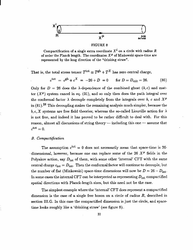
FIGURE 8

Compactification of a single extra coordinate Xi on a circle with radius R of order the Planck length. The coordinates Xp of Minkowski space-time are represented by the long direction of the “drinking straw”.

That is, the total stress tensor Ttot E Tgh + TX has zero central charge,

ctot = Gh+cX = -26+D =0 for D = Dcrit = 26.

Only for D = 26 does the X-dependence of the combined ghost (b, c) and mat-

ter (Xc’) system cancel in eq. (31), and so only then does the path integral over

the conformal factor X decouple completely from the integrals over b, c and Xp

in (81).38 This decoupling makes the remaining analysis much simpler, because the

b, c,X systems are free field theories; whereas the so-called Liouville action for X

is not free, and indeed it has proved to be rather difficult to deal with. For this

reason, almost all discussions of string theory-- including this one - assume that

ctot = 0.

B. Compactijkation

The assumption ctot = 0 does not necessarily mean that space-time is 26-

dimensional, however, because one can replace some of the 26 Xp fields in the

Polyakov action, say Din+, of them, with some other ‘internal’ CFT with the same

central charge tint = Dints Then the conformal factor will continue to decouple, but

the number of flat (Minkowski) space-time dimensions will now be D = 26 - Dint.

In some cases the internal CFT can be interpreted as representing Dint compactified

spatial directions with Planck-length sizes, but this need not be the case.

The simplest example where the ‘internal’ CFT does represent a compactified

dimension is the case of a single free boson on a circle of radius R, described in

section 1II.G. In this case the compactified dimension is just the circle, and space-

time looks roughly like a ‘drinking straw’ (see figure S)..

32

If R is of order the Planck-length, the extra dimension will not be directly

observable by the naked eye, or for that matter by any particle physics experiment

in the near future. However, its presence can affect the spectrum of particles.

To compactify more dimensions, one can use more free bosons (say Dint of them)

living on a Dint-dimensional torus (the product of Dint circles),28 or on some other

appropriate compact manifold.24y25

A simple ‘internal’ CFT which cannot be interpreted literally as a compact-

ification of extra dimensions is the free fermion example of section III.H, or rather

the system of 2Dint free fermions - so that the central charge of the system is an

integer, c = Dint. 26 ._ _

C. Physical States

In order to understand the properties of compactified (or uncompactified)

strings, we first need to describe the physical states. Consider the bosonic string in

the critical dimension D = 26. Because of the gauge symmetry (reparametrization

plus Weyl invariance), not all the states in the (b, c, X) Hilbert space are physical.

This is just as well, because some of them have negative norm, such as afl IO).*

Fortunately, such unphysical states will decouple from the physical, gauge-invariant

states in scattering amplitudes.

There are various ways to identify the gauge-invariant physical subspace of

states. Perhaps the most elegant one is BRST invariance:4gj6 The gauge-fixed

action has a fermionic ‘BRST’ symmetry, for which one can construct an anti-

commuting BRST charge Q satisfying Q2 = 0 and [Q, Lo] = 0. Here Q is given

Q=j & : c(z) (TX(z) + ;Tgh(z)) : . (87) --

Similarly there is a charge & satisfying Q2 = 0, [Q, Lo] = 0, and {Q,&} = 0. (The

condition ctot = 0 is crucial for showing that Q2 = Q2 = 0.) Physical states I$)

are required to satisfy

SW> = gl+> = 0. (88) Note that any state of the form QQ Ix) satisfies eq. (88), so I$) + QQ Ix) is physical

* The Minkowski metric +‘” implicit in the action (4) leads to the commutation relations Ml> a;1 = dn+n,ov”, so that the norm 11 a!1 IO) 112= (Ola$‘cr!I IO) = vpp is negative for the time-like mode.

33

if I$) is. In fact I+) and I$) +Qg Ix) are physically equivalent states for any Ix), so

it is possible to choose any member of this (cohomology) class of states (any x) to

represent a given physical state. In particular, because Q carries ghost number, it

is possible to choose a (virtually) ghost-free representative for each physical state.

For this representative, the conditions (88) only involve the matter (X) part of the

Hilbert space and become, using eq. (87),

Lf 14 = 1 I$> 9 Lc I$) = 0 for n > 0,

E$I$)=ll$), Z~I$)=Oforn>O. W)

But this is just the condition (38) that I$) is a primary state with (h,h) = (1,l).

The dimension (1,l) primary fields that make physical states are called vertex ._ _ operators and are generally denoted by V(z, Z). It is not too surprising that (1,l)

primary fields should make the physical states: To describe a scattering process in

string theory, in which states can be emitted at any point of the world-sheet, one

has to integrate the vertex operators V over their locations on the world-sheet; but

the integral s d2z V(Z,Z) will b e invariant under reparametrizations z + z’ only if

V transforms as a (1,l) primary field.

BRST invariance can also be used to show that the unphysical states (those

which Q does not annihilate) d ecouple from the physical ones in any scattering

process. Basically this is because Q commutes with the ‘Hamiltonian’ Lo, so that

a physical in-state, /@in) with Q I$in) = 0, 1 a wa y s evolves to a physical out-state,

hht) with Q I&& = 0.

Now we can describe explicitly the spectrum of the bosonic string. For

instance, the vertex operator

VT@, q = px(G) (90)

makes a physical state if h = h = L2/2 = 1. The parameter kp in the exponential

is the spacetime momentum of the state. To see this, notice that the momentum

operator Pp that generates space-time translations Xp + Xp + up is

pP = f

dzi&Xcl+ A!!5 27ri f 27ri

i&Xp, (91) and that the eigenvalue of Pp acting on VT is kp (using eq. (57)). Thus the state

Ik) can be identified with a Lorentz-scalar particle of mass mT, where

2 mT = -(C)k2 = -27TT. (92)

(The minus sign comes from our convention for the Minkowski space-time metric

34

rf” = (- + . . . +). Also, we have reinserted the dimensionful string tension T

which was previously set to l/n.)

Equation (92) is rather disturbing because it shows there is a particle with

negative (mass)2, a tachyon, in the bosonic string spectrum. A tachyon is physically

unacceptable; it indicates some kind of instability in the theory. For this reason

the bosonic string is generally considered to be a toy model rather than a viable

string theory. Fortunately, tachyons are not present in the supersymmetric string,

as will be seen in the next section.

The bosonic string states with the next smallest masses (which also appear

in the superstring spectrum) are made by the vertex operators ._ _

The primary state condition (89) restricts the polarization tensor &. Computing

the OPE of Vg with T,

T(z) T/s@4 q - Wh &xu,ik.x(w,Ti7) + 1 + k2/2

(z - Ill)3 w (* _ # K&w) + * - * (94)

(and also with T) one obtains the transversality conditions kp& = ky& = 0

and the mass-shell condition k2 = 0. Thus the states made by V, are massless.

They fall into three different Lorentz multiplets: the graviton gpu (with cclV sym-

metric and traceless), the antisymmetric tensor field B,, (cpV antisymmetric), and

the dilaton 4 (the trace piece of &). Note that the states with time-like polariza-

tion, which we saw to have negative norms, are removed from the physical spectrum

by the transversality condition. The spontaneous appearance of the graviton in the

string spectrum provides one of the principal motivations for studying string the-

ory; it suggests that strings may be a consistent theory of quantum gravity (once

we find a way to remove the tachyon from the spectrum!).

The remaining states in the bosonic string spectrum all have positive masses,

with m2 = (2d!‘)n, n = 1,2,3,. . . They are made by vertex operators like

Vs but with more factors of 8Xp and ax”; hence they form increasingly high

rank tensor representations of the Lorentz group (higher spin particles). Since

their masses are all of order the Planck mass, these particles are not of direct

interest experimentally. However, they do play a key role in radiative corrections

(loops), giving string theory its nice ultraviolet behavior. (Superstrings are free of

35

ultraviolet divergences at one 10op~~j~~, and this finiteness is expected to persist to

all orders in perturbation theory.)

We just described the spectrum of the uncompactified (D = 26) bosonic

string. To construct a compactified spectrum we have to combine the fields r~?‘~,

dXP, 3X” with fields 4 from the internal CFT to make dimension (1,l) vertex

operators V. Every primary field $( z z with conformal dimension (h, h) (a 2d , )

scalar field) gives rise to a space-time-Lorentz scalar particle with mass m 2=

-k2 = (27rT)( h - 1), through the vertex operator V4 = $ ei”x. Higher mass

and spin particles are generated by adding aXp’s and aXv’s to Vd. The most

interesting particles are again usually the massless ones; massless scalars arise only ._ _

from internal fields with (h,h) = (l,l), and massless vectors from fields with

jh,k) = (1,0) or (0,l). F or example, if the internal CFT is a free boson X on

a circle of radius R, I$ = 8X8X leads to a massless scalar and dX, 3X lead to

massless vectors. (The partition function (71) f or the circle CFT shows that for

special values of R there can be additional massless vectors and scalars, obtained

from vertex operators of the form e ~(~LXL+~RXR).)

V. SUPERSTRINGS AFD INTERACTIONS:

A. Superstrings and Superconformal Invariance

As we have seen, the bosonic string is an unacceptable theory because of its

tachyon, but it is also phenomenologically unacceptable as a unified theory because

it has no spacetime fermions in its spectrum. To remedy the situation, we now de-

scribe the superstring, which incorporates space-time supersymmetry and therefore

leads to a fermionic state for each bosonic state. (Of course, for phenomenologi-

cal reasons space-time supersymmetry must be spontaneously broken at an energy

scale of at least the weak scale (M 100 GeV).) Th ere are two different descriptions

of the superstring. In the Green-Schwarz 2o (GS) f ormulation space-time supersym-

metry is manifest, but Lorentz covariance is hard to maintain in the quantization

procedure. I will d escribe here instead the Neveu-Schwarz-Ramond18 (NSR) for-

mulation, in which space-time supersymmetry is obscure, but Lorentz covariance

can be maintained. (The description will be rather sketchy in any case.)

The action used in the NSR formulation is37

36

where ~1 = 0,1,2 ,... , D - 1 is a space-time index and Q, ,8 = 0,l are world-sheet

indices as before. This action has a supersymmetry, but it is a local world-sheet

pa) supersymmetry,

-- - be: = -2iVyaxa,

kya = Vc&

rather than a space-time supersymmetry. Here Qp are D two-component Majorana

fermions (equivalent to D of the spinors Ik discussed in section III.H), which are

the superpartners of Xp; xa is a world-sheet gravitino field, the superpartner of

the 2d metric gap; and e, (y is the zweibein for the metric, satisfying eaea - g a@- ap ,

e E- det(eg) = J-s. In addition to having all the symmetries of the Polyakov

action, plus (96), the action (95) h as a symmetry transforming only the gravitino

field, s rlX& = iyd,

(97) - S,e = S,Gp = S,Xp = 0.

Both E and q are infinitesimal, anticommuting 2d spinors.

The path integral of interest is now38

Z = (98)

We again use the Fadeev-Popov procedure to gauge-fix the local symmetries of the

action (95) in the path integral, choosing

xa = 0 (99)

in addition to the conformal gauge choice (76) for the metric. The integration over

metrics g,p is traded for an integral D[ DA as before, and the integration over the

37

gravitino X~ is traded for DcDq. Since 6x(, = Vae, the Jacobian for the change of

variables in the Grassmann gravitino path integral is

J = (det(Gx,/Sc))-’ - (det 0,)-l . (det VT)-‘. (100)

In this case, the operators VT and V, act on spinors (E.) rather than the vectors

(0 of the bosonic Jacobian. The determinants are therefore represented’ as path

integrals over commuting fields with half-integer dimensions (ghosts), p, y and p, 7

with hp = 312, h, = -l/2,

(det VT)-’ = / WW exp (-i/d22 K-b) y (lol)

(det 0,)-l = J

nDi?eexp (-i/d2z B&T).

The P,r system is another example of the general 8,e system discussed in

section IV.A, with j = 3/2 and stress tensor

TPr = -; P&r - &3)y (102)

Since /?,r commute, the central charge computation (85) gives $7 = +ll. The

gauge-fixed action for the ‘matter fields’ Xp and !Pp = ($P qP)T is

Sgf = -& jd2z {dzXp+Xp + $p+$p +~p&~p}. (103)

The central charge for this system is D(1 + 4). Thus the total (ghost plus matter)

stress tensor Ttot = TbC + TP7 + TX + T$ has central charge

ctot = $c + cP7 + cx + 8 = -26 + 11 + D(1 + ;) = $(D - lo), (104)

which vanishes if D = 10. As in the bosonic case, the conformal factor X decouples

.only in this dimension. 38 So superstrings pick out Dcrit = 10 as their critical

dimension.

The gauge-fixed action (103) h as an important residual symmetry besides

just conformal invariance, namely superconformal invariance,50 which is the gauge-

fixed version of the local supersymmetry (96):

sxp = e7y + $,

s?y = ea*xy (105)

&p = &Xc”.

In the same way that the fields T(z) and T(F) g enerate conformal transformations,

superconformal transformations are generated by a pair of fields TF(z) and Tp(Z),

38

which are the superpartners of T and T. For the Xp,$p,$’ system of (103), the

superconformal generator is

The

be

OPEs of T(z), TF( z are determined by superconformal symmetry to )

T(z)T(w) - 3”4 2T(w) 8,T

(* - w)4 + (z - w)2 + 2 - w + “”

t/4 TFb) TF(w) - cz _ w)2 +

w)T(~) + z-u) ****

(107)

The first line of (107) is just the usual stress tensor OPE, with C defined to be

2 = ic. (The reason for this definition is so that the system (X, $J) of a single free

boson plus its fermionic superpartner has C = $(l+ a) = 1.) The second line states

that TF is a dimension 3/2 holomorphic primary field. The third line is required by

the fact that superconformal transformations close into conformal transformations. -- --

The fields T,TF obey the same algebra with z,w --t 2,~. As usual, TF can be

expanded into Laurent modes, according to -

TF(z) = C $G, zere3i2,

?G+; (10s)

G,. = f

& ~TF(z) zn+‘j2.

-The algebra obeyed by the modes L, and G, is called the superconformal algebra.

The full algebra (107), with c = c(xy@) = 15 or 2 = C(xl$) = 10, is required to

show that the path integral over the field q decouples (whereas the first line of (107)

suffices to show decoupling of the conformal factor X). Thus to ‘compactify’ Dint

dimensions in a superstring theory, we replace a system Xp, $@“, v’ by an internal -int _ superconformal field theory with the same central charge, c - Dint.

Physical states in the superstring Hilbert space can again be identified using

BRST invariance. There are several additional subtleties having to do with the

commuting ,0,r ghosts, which I will not go into here.’ A physical state that is a

space-time boson has a (virtually) ghost-free representation (as in the case of the

39

bosonic string). A state 140) in this representation is required by BRST invariance

to be a ‘primary state’ with respect to the full superconformal algebra, not just

the Virasoro algebra; that is, 1~~50) must be annihilated by the positive-frequency

modes of both T and TF:

JL 140) = 0, 7-6 L 1, Lo MO> = h 140) 7 G 140) = 0, r 2 i (r E Z + l/2), G-1/2 140) = I&> - (109)

The new state 141) appearing in (109) is the 2d superpartner of I&), and is primary

under the conformal algebra with dimension h + l/2. The fields $0, $1 that make

the states 140) , I#4 f orm a 2d primary superfield of dimension h; $0 is the lower

component of the superfield and ~$1 is the upper component. Their OPEs with T

and TF are fixed by eq. (109) and superconformal symmetry to be

2TF(z)+O(w>;iir) - 41h w

+..., Z-W

2TF@> hb, w> - 2Wo(w, W

(2 - wy + aldo +

z-w “”

(110) TW $o(w, 3 N Mob, E’> + dud0 +

(z-w)2 z-w “”

(h + 1’3#4w,=) + awh + T(z) 41 (w, 4 N (z - wy 2-w ****

A vertex operator for a bosonic superstring state is actually the upper com-

ponent 41 of a dimension h = l/2 (also x = l/2) p rimary superfield. Such a field 41

is primary with respect to T alone, and has conformal dimension h + l/2 = 1 (and

h+ 1’2 = 1), so the physical state restrictions for the superstring are a superset of

those for the bosonic string. (Of course the initial Hilbert space is larger for the

superstring due to the additional fields tip,?‘.) It is usually easiest to construct

the vertex operators by first finding the lower components 40, then applying TF to

them to obtain 41 (using eq. (110)):

h(w,E) = ;$w(Z - W@T~(z))do(w,~). (111)

There is one more requirement on ~$1 for it to describe a physical state: It must

have even fermion number F, where F = $ & $~(z)$~(z) counts the number

of $Y fields in a vertex operator, and F = $ & F’(z)?~(z) must also be even.

40

This requirement is known as the GSO projection, and it leads to a space-time

supersymmetric mass spectrum. 19

Now let’s look at the lowest mass bosonic states. The field $0 = eilc’x is

primary under the superconformal algebra with h = k2/2. However, the upper

component, obtained using (111) and a similar limit with FF, is i k . II, ik . TeikeX

and has odd fermion numbers F and F, so it is not a physical state. This is just

as well, because it would have been a tachyon, with m2 = -k2 = -1.

The lowest mass physical states are obtained from the field ~PV~~~Veilc’x,

which is the lowest component of a primary superfield if cPV satisfies the same

transversality condition as in the bosonic string case and if k2 = 0. Applying TF -_ _ and TF and checking that F,F are even, one gets

The vertex operators (112) are just the superstring version of (93); they again give

rise to a graviton, an antisymmetric tensor and a dilaton in the massless spectrum.

The construction of vertex operators for space-time fermions in the NSR

formulation is more subtle,51t6 and requires a better understanding of the P,r

ghost system than I have given here. The main difference from the bosonic vertices

is that the fermionic vertices have a square-root singularity with respect to Tp.

That is, if such a vertex operator is located at the origin z = 0, then the Laurent

expansion of TF(z) is in terms of integer rather than half-integer modes,

TF(z) = c G,z -n-3/2 , (113)

nEZ

-

-and Gn must annihilate the state for n > 0. Also, the vertex operators (in one

choice of ghost representation) must have dimension 5/S. Such fields exist in the

$p”, $? conformal field theory; they are called spin fields, are denoted by C” and

II’, and have square-root singularities with the world-sheet fermions $@“, qP. Here

Q! and & are ten-dimensional Lorentz spinor indices. Thus the vertex operators

Vgravitino = ~paCa(z)(~X~ + ik . @‘) e’c’x,

V’ gravitino = &JF’(F)(&X~ + ik . $u,!P) eik’X, (114)

carry both vector and spinor indices an give rise to gravitinos (spin-312 particles)

in the massless spectrum. The presence of gravitinos implies that the theory should

be space-time supersymmetric, and indeed it is.51l6

41

The spectrum for a compactified version of the superstring can be found

in similarly. As in the bosonic case, fields eik’x, $P, dXr-l, etc. from the space-

time part of the theory are combined with fields from the internal (super)conformal

theory to make vertex operators, with the additional restrictions that the combined

vertex operators (for space-time bosons) must be upper components of superfields,

and must be even under a generalized GSO projection.

B. Heterotic Strings

We have seen how the introduction of world-sheet supersymmetry and the

GS_Q projection has led to a superstring with no tachyon and with massless fermions

(indeed, with space-time supersymmetry), which are two steps towards obtaining a

spectrum that might include the standard model spectrum. Still missing, however,

are gauge bosons. They are in fact rather difficult to obtain from the superstring

just described, even when it is compactified. 3o152 So we now briefly describe the

one remaining theory of closed superstrings, namely the heterotic string.23

The heterotic string is a hybrid of the bosonic string and the superstring

just discussed. Essentially, the antiholomorphic, or left-moving, degrees of freedom

are taken to be those of the bosonic string, and the holomorphic, or right-moving,

degrees of freedom are those of the superstring. That is, the 2d conformal field

theory for the heterotic string has a right-moving superconformal invariance gen-

erated by a field TF, but no left-moving superconformal invariance (no TF). The

same arguments as were applied above to the bosonic string and the superstring

would now seem to imply that the critical dimension for the heterotic string is both

.26 (the bosonic calculation) and 10 (the superstring calculation)!

This paradox is resolved by ‘compactifying’ 16 of the dimensions of the

bosonic part of the heterotic string; that is, one replaces 16 of the directions

Xp by an internal conformal field theory with central charge C = 16 and c = 0.

Since c = 0, this internal CFT is trivial in its z-dependence (all fields have right-

moving dimension h = 0, and so they are independent of z), so it is called an

‘(anti)holomorphic conformal field theory’. It turns out that there are only two

such theories with -E = 16. Both of them turn out to have exactly 498 primary

fields J”(Z), a = 1,2,. . .498, of dimension x = 1. The fields 3” are important be-

cause they give rise to 498 gauge bosons in the massless spectrum of the heterotic

42

string. The gauge boson vertex operators are

VA(Z,z) - $(&X” + ik - $n,P) J”(Z) eik*X(rpH),

where k2 = 0 and the polarization vector $ is transverse, kp<,tj = 0. Note that

VA is the upper component of a dimension h = l/2 superfield ($peikeX) for the

right-moving superconformal algebra, and is a dimension x = 1 conformal field

thanks to KT = 1. The gauge group depends on the properties of the J”, and

turns out to be either I$3 x Es or SO(32), depending on which of the two C = 16

antiholomorphic CFTs is used.

The heterotic string also has in its massless spectrum a graviton, antisym-

met% tensor, dilaton, and superpartners of all of these. The corresponding vertex

operators are the same as those (112),(114) of th e superstring in their z-dependence,

and the same as the graviton vertex operator (93) of the bosonic string in their

Z-dependence. For example,

with kp&,, = k”<pv = 0, k2 = 0. The superpartners of the gauge bosons are

gauginos, massless fermions. transforming under the adjoint representation of Es x

I38 or SO(32). Wh en one tries to make contact between some four-dimensional

version of the heterotic string and the standard model, one usually identifies the

gauge group SU(3), x sum x U(l)y with a subgroup of Es x E&J. Then some

components of the ten-dimensional gauginos become four-dimensional gauginos

(superpartners of the standard model gauge bosons); but other components have

the proper gauge quantum numbers to be identified with the fermions (quarks and

-1eptons) of the standard mode1.24

To see whether such an identification is viable, one must first understand how

to construct four-dimensional versions of the heterotic string. These compactifica-

tions are described by internal superconformal theories with c = 9 and c = 22 (we

absorb the F = 16 system into the internal CFT); only a right-moving supercon-

formal invariance needs to be present, as was true of the uncompactified heterotic

string. The additional restrictions on physical vertex operators that were found

for the superstring also apply to the heterotic string, but only to the right-moving

degrees of freedom. There are now many different schemes for constructing four-

dimensional heterotic strings, 24~25~26y27 which all fall under the general approach

43

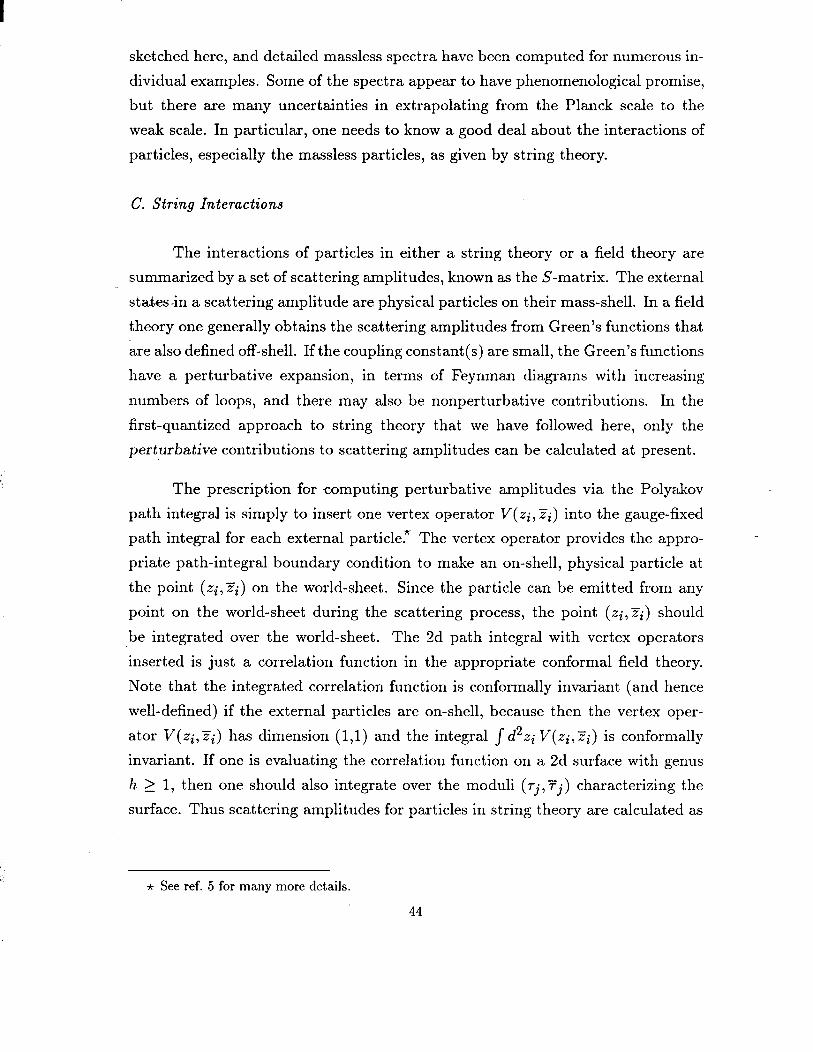
sketched here, and detailed massless spectra have been computed for numerous in-

dividual examples. Some of the spectra appear to have phenomenological promise,

but there are many uncertainties in extrapolating from the Planck scale to the

weak scale. In particular, one needs to know a good deal about the interactions of

particles, especially the massless particles, as given by string theory.

C. String Interactions

The interactions of particles in either a string theory or a field theory are

summarized by a set of scattering amplitudes, known as the S-matrix. The external

states-in a scattering amplitude are physical particles on their mass-shell. In a field

theory one generally obtains the scattering amplitudes from Green’s functions that

are also defined off-shell. If the coupling constant(s) are small, the Green’s functions

have a perturbative expansion, in terms of Feynman diagrams with increasing

numbers of loops, and there may also be nonperturbative contributions. In the

first-quantized approach to string theory that we have followed here, only the

perturbative contributions to scattering amplitudes can be calculated at present.

The prescription for computing perturbative amplitudes via the Polyakov

path integral is simply to insert one vertex operator V(zi,Zi) into the gauge-fixed

path integral for each external particle.* The vertex operator provides the appro-

priate path-integral boundary condition to make an on-shell, physical particle at

the point (zi,Zi) on the world-sheet. Since the particle can be emitted from any

point on the world-sheet during the scattering process, the point (zi, YZi) should

be integrated over the world-sheet. The 2d path integral with vertex operators

inserted is just a correlation function in the appropriate conformal field theory.

Note that the integrated correlation function is conformally invariant (and hence

well-defined) if the external particles are on-shell, because then the vertex oper-

ator V(zi,Zi) has dimension (1,l) and the integral s d2zi V(zi,Ti) is conformally

invariant. If one is evaluating the correlation function on a 2d surface with genus

h 2 1, then one should also integrate over the moduli (rj, ~j) characterizing the

surface. Thus scattering amplitudes for particles in string theory are calculated as

--

A- See ref. 5 for many more details.

44

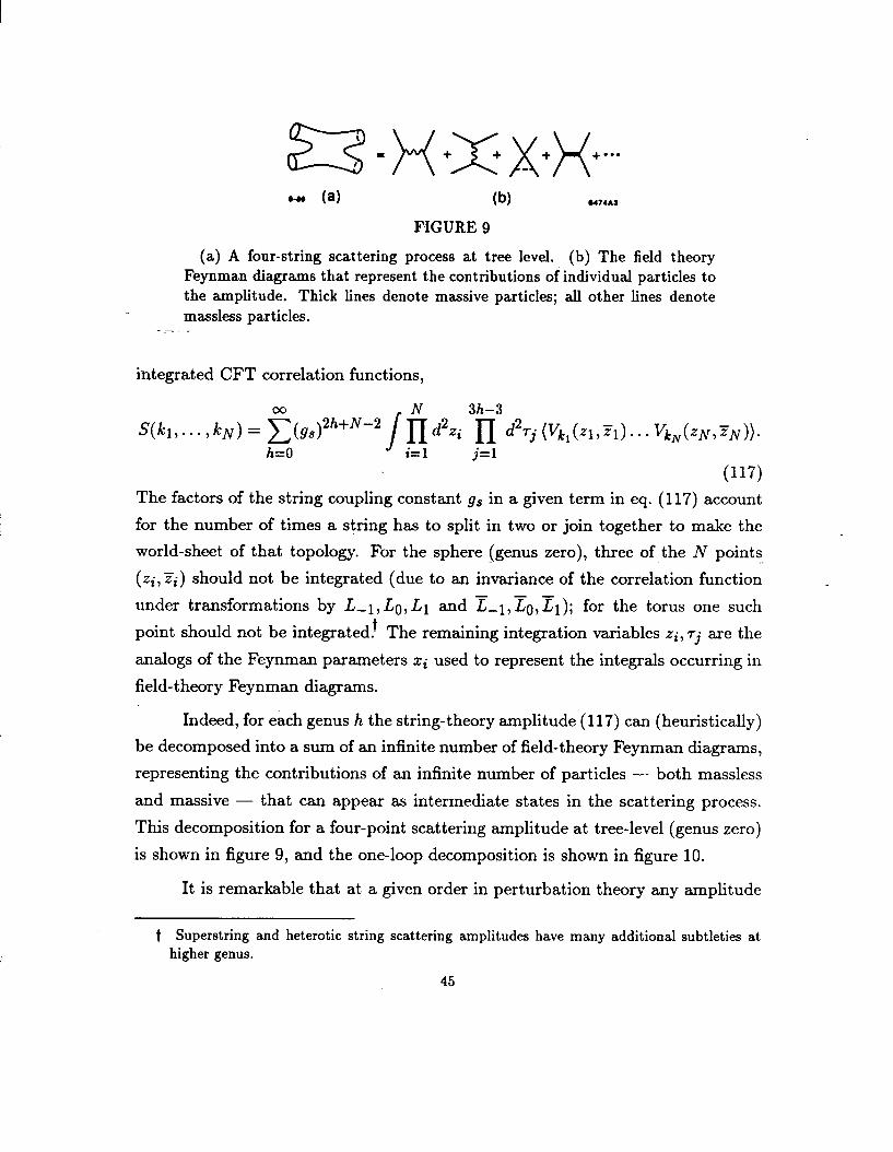
- (a) (W

FIGURE 9

(a) A four-string scattering process at tree level. (b) The field theory Feynman diagrams that represent the contributions of individual particles to the amplitude. Thick lines denote massive particles; all other lines denote massless particles.

._ _

i-ntegrated CFT correlation functions,

S(kl,. . . , kN) = c(gs)2h+N-2 d2q (Yk,(Zl7Fl) - * - h&N,%). h=O

(117)

The factors of the string coupling constant gs in a given term in eq. (117) account

for the number of times a string has to split in two or join together to make the

world-sheet of that topology. For the sphere (genus zero), three of the N points

(zi,~i) should not be integrated (due to an invariance of the correlation function

under transformations by L-1, Lo, L1 and E-1, &,&); for the torus one such

point should not be integrated! The remaining integration variables zi, rj are the

analogs of the Feynman parameters zi used to represent the integrals occurring in

field-theory Feynman diagrams.

Indeed, for each genus h the string-theory amplitude (117) can (heuristically)

be decomposed into a sum of an infinite number of field-theory Feynman diagrams,

representing the contributions of an infinite number of particles - both massless

and massive - that can appear as intermediate states in the scattering process.

This decomposition for a four-point scattering amplitude at tree-level (genus zero)

is shown in figure 9, and the one-loop decomposition is shown in figure 10.

It is remarkable that at a given order in perturbation theory any amplitude

t Superstring and heterotic string scattering amplitudes have many additional subtleties at higher genus.

45

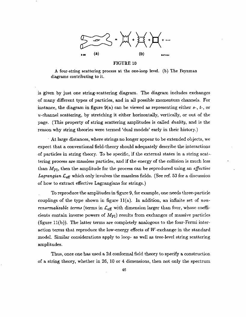
FIGURE 10

A four-string scattering process at the one-loop level. (b) The Feynman diagrams contributing to it.

is given by just one string-scattering diagram. The diagram includes exchanges

of many different types of particles, and in all possible momentum channels. For

instance, the diagram in figure 9(a) can be viewed as representing either s-, t-, or

u-channel scattering, by stretching it either horizontally, vertically, or out of the

page. (This property of string scattering amplitudes is called duality, and is the

reason why string theories were termed ‘dual models’ early in their history.)

At large distances, where strings no longer appear to be extended objects, we

expect that a conventional field-theory should adequately describe the interactions

of particles in string theory. To be specific, if -the external states in a string scat-.

tering process are massless particles, and if the energy of the collision is much less

than Mpl, then the amplitude for the process can be reproduced using an efiective

Lagrungian L,ff which only involves the massless fields. (See ref. 53 for a discussion

of how to extract effective Lagrangians for strings.)

-

To reproduce the amplitudes in figure 9, for example, one needs three-particle

couplings of the type shown in figure 11(a). In addition, an infinite set of non-

renormahable terms (terms in & with dimension larger than four, whose coeffi-

cients contain inverse powers of Mpl) results from exchanges of massive particles

(figure 11(b)). The latter terms are completely analogous to the four-Fermi inter-

action terms that reproduce the low-energy effects of W-exchange in the standard

model. Similar considerations apply to loop- as well as tree-level string scattering

amplitudes.

Thus, once one has used a 2d conformal field theory to specify a construction

of a string theory, whether in 26, 10 or 4 dimensions, then not only the spectrum

46

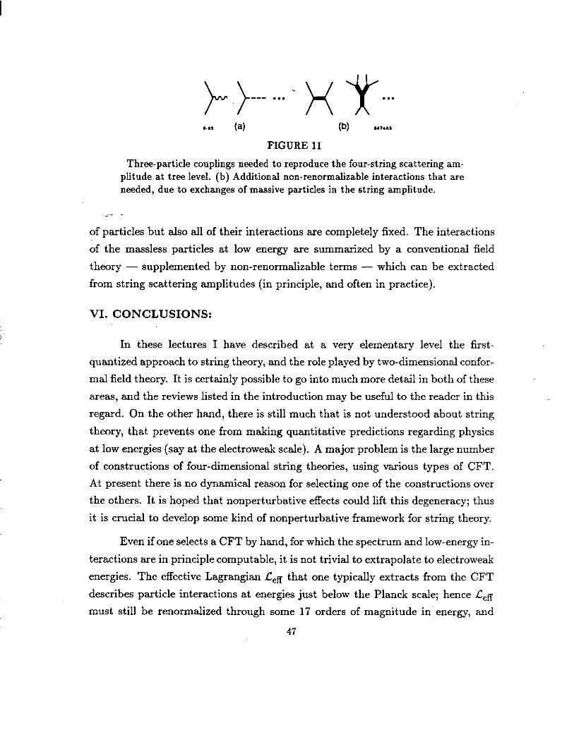
p }--- . . . - x y . . . (a) (b) “I4Al

FIGURE 11

Three-particle couplings needed to reproduce the four-string scattering am- plitude at tree level. (b) Additional non-renormalizable interactions that are needed, due to exchanges of massive particles in the string amplitude.

of particles but also all of their interactions are completely fixed. The interactions

of the massless particles at low energy are summarized by a conventional field

theory - supplemented by non-renormalizable terms - which can be extracted

from string scattering amplitudes (in principle, and often in practice).

VI. CONCLUSIONS:

In these lectures I have described at a very elementary level the first-

quantized approach to string theory, and the role played by two-dimensional confor?

mal field theory. It is certainly possible to go into much more detail in both of these

areas, and the reviews listed in the introduction may be useful to the reader in this

regard. On the other hand, there is still much that is not understood about string

theory, that prevents one from making quantitative predictions regarding physics

at low energies (say at the electroweak scale). A major problem is the large number

of constructions of four-dimensional string theories, using various types of CFT.

At present there is no dynamical reason for selecting one of the constructions over

the others. It is hoped that nonperturbative effects could lift this degeneracy; thus

it is crucial to develop some kind of nonperturbative framework for string theory.

Even if one selects a CFT by hand, for which the spectrum and low-energy in-

teractions are in principle computable, it is not trivial to extrapolate to electroweak

energies. The effective Lagrangian &.ff that one typically extracts from the CFT

describes particle interactions at energies just below the Planck scale; hence f&

must still be renormalized through some 17 orders of magnitude in energy, and

47

possibly through several intermediate regimes of symmetry-breaking. Of the many

uncertainties in this process, perhaps the greatest is in the mechanism of space-time

supersymmetry breaking, which is (in the usual scenarios) ultimately responsible

for the enormous hierarchy between the Planck scale and the electroweak scale, and

which also can feed into predictions for other measured parameters of the standard

model (quark and lepton masses, etc.). It seems that supersymmetry breaking

should be nonperturbative, in order to generate the observed hierarchy. One might

hope that it is a long-distance effect that could be calculated using an effective La-

grangian, for which nonperturbative tools are already available. To date, however,

no proposed supersymmetry-breaking mechanism has led to a particularly realistic

out-come.

In summary, while string theory is currently the leading candidate for a

consistent theory of quantum gravity, the question of whether or not it can also

generate definite predictions of low-energy phenomena is still open, and awaits the

development of further calculation tools, or conceptual understanding, or both.

ACKNOWLEDGMENTS:

I would like to thank-the organizers of TASI-89, the students, and the sur-

rounding mountains for a thoroughly enjoyable time, and Jan Louis for many useful

comments on the manuscript.

REFERENCES:

1. E. Martinet, in Proc. of the 1987 ICTP Spring School on Supersymmetry, Supergrav- ity and Superstrings, eds. L. Alvarez Gaumd, M.B. Green, M. Grisaru, R. Jengo and E. Sezgin (World Scientific, 1987).

2. T. Banks, in The Santa Fe TASI 87 Proceedings, eds. R. Slansky and G. West (World Scientific, 1988).

3. P. Ginsparg, lectures at Les Houches summer session, 1988, to appear in Chumps, Cordes et Phe’nomGnes Critiques: Fields, Strings and Critical Phenomena, eds. E. Br6zin and J. Zinn-Justin (Elsevier, 1989).

4. J. Cardy, lectures at Les Houches summer session, 1988, to appear in Chumps, Cordes et Phe’nomGnes Critiques: Fields, Strings and Critical Phenomena, eds. E. Brbzin and J. Zinn-Justin (Elsevier, 1989).

5. M.B. Green, J.H. Schwarz and E. Witten, Superstring Theory, Vols. I and II (Cam- bridge University Press, 1987).

6. D. Friedan, E. Martinet and S. Shenker, Nucl. Phys. B271, 93 (1985).

48

7. M. Peskin, in From the Planck Scale to the Weak Scale: Towards a Theory of the Universe (Santa Cruz TASI 86 Proceedings), ed. H.E. Haber (World Scientific, 1987).

8. L. Dixon, in Proc. of the 1987 ICTP Summer Workshop in High Energy Physics and Cosmology, Trieste, Italy, eds. G. Furlan, J.C. Pati, D.W. Sciama, E. Sezgin and Q. Shafi (World Scientific, 1988).

9. J.H. Schwarz, ht. J. Mod. Phys. A4, 2653 (1989).

10. W. Lerche, A. Schellekens and N. Warner, Phys. Repts. 177, 1 (1989).

11. M. Kaku, Introduction to Superstrings (Springer-Verlag, 1988).

12. M. Dine, in String Theory in Four Dimensions, Current Physics Sources and Com- ments, Vol. I, ed. M. Dine (North-Holland, 1988).

13. A. Schehekens, in Super-string Construction, Current Physics Sources and Comments, .._ Vol. IV, ed. A. Schellekens (North-Holland, 1989).

14. Y. Nambu, in Symmetries and Quark Models, ed. R. Chand (Gordon and Breach, 1970); H.B. Nielsen, submitted to the 15th Int’l Conf. on High Energy Physics (Kiev, 1970); L. Susskind, Nuovo Cim. 69A, 457 (1970).

15. N. Isgur, “Hadron Spectroscopy: An overview with Strings Attached”, Toronto preprint UTPT-89-13 (1989), and references therein.

16. X. Artru and G. Mennessier, Nucl. Phys. B70, 93 (1974); M.G. Bowler, 2. Phys. Cll, 169 (1981); D. Morris, Nucl. Phys. B313, 634 (1989).

17. J. Scherk and J.H. Schwarz, Nucl. Phys. B81, 118 (1974); Phys. Lett. 57B, 463 (1975).

18. P. Ramond, Phys. Rev. D3, 2415 (1971); A. Neveu and J.H. Schwarz, Nucl. Phys. B31, 86 (1971).

19. F. Gliozzi, J. Scherk and D. Olive, Phys. Lett. 65B, 282 (1976), Nucl. Phys. B122, 253 (1977).

20. M.B. Green and J.H. Schwarz, Nucl. Phys. B181, 502 (1981), Nucl. Phys. B198, 252 (1982).

21. M.B. Green and J.H Schwarz, Phys. Lett. 109B, 444 (1982).

22. M.B. Green and J.H. Schwarz, Phys. Lett. 149B, 117 (1984).

23. D. Gross, J. Harvey, E. Martinet and R. Rohm, Phys. Rev. Lett. 54, 502 (1985): Nucl. Phys. B256, 253 (1985), Nucl. Phys. B267, 75 (1986).

24. P. Candelas, G. Horowitz, A. Strominger and E. Witten, Nucl. Phys. B258, 46 (1985).

25. L. Dixon, J. Harvey, C. Vafa and E. Witten, Nucl. Phys. B261, 620 (1985), Nucl. Phys. B274, 285 (1986).

26. H. Kawai, D. LewelIen and S.-H.H. Tye, Phys. Rev. Lett. 57, 1832 (1986), Nucl. Phys. B288, 1 (1987).

49

27. L.E. Ibafiez, H.P. Nilles and F. Quevedo, Phys. Lett. 187B, 25 (1987); L.E. Ibaflez, J.E. Kim, H.P. Nilles and F. Quevedo, Phys. Lett. 191B, 3 (1987); A. Chamseddine and J.-P. Derendinger, Nucl. Phys. B301, 381 (1988); K.S. Narain, M.H. Sarmadi and C. Vafa, Nucl. Phys. B288, 551 (1987); W. Lerche, D. Lust and A. ScheIIekens, Nucl. Phys. B287, 477 (1987); D. Gepner, Phys. Lett. 199B, 380 (1987), Nucl. Phys. B296, 757 (1988); Y. Kazama and H. Suzuki, Nucl. Phys. B321, 232 (1989), Phys. Lett. 216B, 112 (1989); I. Antoniadis, C. Bachas and C. Kounnas, Nucl. Phys. B289, 87 (1987); I. Antoniadis, J. Ellis, J.S. Hagelin and D.V. Nanopoulos, preprint CERN- TH.5442/89.

28. M.B. Green, J.H. Schwarz and L. Brink, Nucl. Phys. B198, 474 (1982).

29. D. Friedan, Phys. Rev. Lett. 45, 1057 (1980), Ann. of Phys. 163, 318 (1985); C. Lovelace, Phys. Lett. 135B, 75 (1984), Nucl. Phys. B273, 413 (1986);

---- E. Fradkin and A.A. Tseytlin, Phys. Lett. 158B, 316 (1985), Phys. Lett. 16OB, 64 (1985), Nucl. Phys. 261B, 1 (1986); C. Callan, D. Friedan, E. Martinet and M. Perry, Nucl. Phys. B262, 593 (1985); A. Sen, Phys. Rev. Lett. 55, 1846 (1985), Phys. Rev. D32, 2102 (1985).

30. D. Friedan, Z. Qiu and S. Shenker, in Proc. 1984 Santa Fe Meeting of APS Div. Particles and Fields Conf., eds. T. Goldman and M. Nieto (World Scientific, 1985).

31. A.M. Polyakov, J.E.T.P. Lett., 12, 381 (1970).

32, A.B. Zamolodchikov, J.E.T.P. Lett., 46, 160 (1987), and lectures at the Taniguchi Conference on Integrable Models, Kyoto, Japan, 1988.

33. E. Witten, Comm. Math. Phys. 117, 353 (1988).

34. For a review, see G. Moore and N. Seiberg, lectures given at Trieste, Italy and Banff, Canada, preprint RU-89-32 (1989).

35. See W. Siegel, Introduction to String Field Theory (World Scientific, 1988).

36. Y. Nambu, lectures at the Copenhagen symposium (1970); 0. Hara, Prog. Theor. Phys. 46, 1549 (1971); T. Goto, Prog. Theor. Phys. 46, 1560 (1971).

37. S. Deser and B. Zumino, Phys. Lett. 65B, 369 (1976); L. Brink, P. DiVecchia and P. Howe, Phys. Lett. 65B, 471 (1976).

38. A.M. Polyakov, Phys. Lett. 103B, 207 (1981), Phys. Lett. 103B, 211 (1981).

39. A.A. Belavin, A.M. Polyakov and A.B. Zamolodchikov, Nucl. Phys. B241, 333 (1984).

40. J. Polchinski, Nucl. Phys. B303, 226 (1988).

41. K. Wilson, in Proc. Midwest Conf. on Theoretical Physics, Notre Dame, Ind. (1970); W. Zimmermann, in Lectures on Field Theory and Elementary Particles, eds. H. Pendleton and M. Grisaru (MIT Press, 1970).

42. M. Virasoro, Phys. Rev. Dl, 2933 (1970).

43. D. Friedan, Z. Qiu and S. Shenker, Phys. Rev. Lett. 52, 1575 (1984).

50

44. V1.S. Dotsenko and V.A. Fateev, Nucl. Phys. B240[FS12], 312 (1984), Nucl. Phys. B251[FS13], 691 (1985), Phys. Lett. 154B, 291 (1985).

45. J. Cardy, Nucl. Phys. B270[FSl6], 186 (1986).

46. See for example G. Springer, Introduction to Riemann Surfaces (Addison-Wesley, 1957).

47. D. Gepner and E. Witten, Nucl. Phys. B278, 493 (1986); D. Gepner, Nucl. Phys. B287, 111 (1987); A. Cape& C. Itzykson and J.-B. Zuber, Nucl. Phys. B280[FS18], 4455 (1987), Comm. Math. Phys. 113, 1 (1987).

48. 0. Alvarez, Nucl. Phys. B216, 125 (1983); in Unified String Theories, eds. M.B. Green and D. Gross (World Scientific, 1986).

49. C. Becchi, A. Rouet and R. Stora, Phys. Lett. 52B, 344 (1974), Ann. Phys. 98, 287 --- (-1976).

50. A. Neveu, J.H. Schwarz and C.B. Thorn, Phys. Lett. 35B, 529 (1971); J.L Gervais and B. Sakita, Nucl. Phys. B34, 632 (1971).

51. D. Friedan, E. Martinet and S. Shenker, Phys. Lett. 160B, 55 (1985); V.G. Knizhnik, Phys. Lett. 160B, 403 (1985).

52. L. CasteIIani, R. D’Auria, F. Gliozzi and S. Sciuto, Phys. Lett. 168B, 47 (1986); R. Bluhm, L. Dolan and P. Goddard, Nucl. Phys. B289, 364 (1987); H. Kawai, D. Lewellen and S.-H.H. Tye, Phys. Lett. 191B, 63 (1987); L. Dixon, V. Kaplunovsky and C. Vafa, Nucl. Phys. B294, 43 (1987).

53. D. Gross and J. Sloan, Nucl. Phys. B291, 41 (1987).

51