Theory of conformal optics Study of classical optics via conformal invariants

Amin Vahdat Farimani

2/17/2015

Gmail: aminvahdat79@gmail.com

A simple mathematical tool is presented for study of classical optics via conformal invariants. In math, Erlanger program conceives geometry as study of invariants properties under a group of transformations. Theory of conformal optics should be considered as an Erlanger program for study of classical optics when conformal mappings are selected as transformations.

Abstract

A simple mathematical tool is presented for study of classical optics via conformal invariants. In math,

Erlanger program conceives geometry as study of invariants properties under a group of

transformations. Theory of conformal optics should be considered as an Erlanger program for study of

classical optics when conformal mappings are selected as transformations.

Keywords

Conformal optics, refraction, reflection, diffraction, interference, cross ratio, Poincare disk model, unit

disk

Introduction

Felix Klein (1849-1925) in his “Erlanger program” presented a new definition for geometry “study of

invariants properties under a group of transformations”. Transformations are called conformal

mappings when angles remain unchanged under mappings. As Klein definition for geometry, conformal

optics should be defined. It is study of properties of optical phenomena which are invariant under

conformal mappings. In present paper a variety of optical phenomena will be analyzed by use of one

fundamental axiom.

In section-1 fundamental axiom of the conformal optics will be presented.

In section-2, section-3 and section-4 refraction, reflection and interference phenomena will be analyzed

respectively.

Diffraction is subject of section-5. In all sections the fundamental axiom plays central role. In section-5

an auxiliary concept is presented to develop cross ratio. In other words the Poincare disk model for the

hyperbolic geometry is generalized to a variety of conformal non-Euclidean models. These conformal

models are needed for quantitative analyzing of diffraction phenomenon.

The last section-6 is conclusion.

Section-1 (Fundamental axiom)

When an optical phenomenon occurs, there is at least one non-zero quanta property which is invariant

under conformal mappings from phenomenon scene to the unit disk. (See fig.1) In fig.1 point “S”

denotes to source of light, 𝑍1 and 𝑍2 to slots and 𝑍3 to position of Geiger counter. Also “C” refers to

boundary of phenomenon scene.

phenomenon unit disk

s

Z1

Z3

Z2

w1

w2w3

mapping

scene

C

fig.1: Mapping from phenomenon scene to the unit disk

Section-2 (Refraction phenomenon)

L1

L2

media 1

media 2boundary

i

r

L ( normal to boundary )

fig.2: Refraction scene

According to the fundamental axiom we are sure that one non-zero property for refraction phenomenon

exists. Let examine cross ratio (L1 , L2; L) as property of refraction. (See appendix-1)

(𝐿1 ,𝐿2; 𝐿) = sin∠𝐿1𝐿 sin∠𝐿2𝐿 = sin(𝜋 − 𝑖) / sin(𝜋 − 𝑟) = sin 𝑖 sin 𝑟 1

Since cross ratio is invariant under conformal mapping then invariance of “sin 𝑖 sin 𝑟 ” is property of

refraction. It means that

sin 𝑖 sin 𝑟 = 𝑐𝑜𝑛𝑠𝑡𝑎𝑛𝑡 2

Section-3 (Reflection phenomenon)

L1 media 1 media 2

boundary

i

L ( normal to boundary )L ( normal to boundary )

L1

r

fig.3: Reflection scene

According to the fundamental axiom we are sure that one non-zero property for reflection phenomenon

exists. Let examine cross ratio (L1 , L2; L) as property of reflection.

(L1 , L2; L) =sin∠L1L sin∠L2L = sin(π − i) / sin(π − r) = sin i sin r = constant 3

From symmetry we expect that when L1 is parallel to Σ, L2 is also parallel to Σ. It means that from

(i = π 2) we conclude the(r = π 2 ). So from 3 we obtain sin i / sin r = 1 or

𝑖 = 𝑟 4

Equation 4 is property of reflection.

Section-4 (Interference phenomenon)

boundary

s

L1

L

L2

Fig.4: Interference scene (S shows Light source; L1 and L2 show slots; L shows Geiger counter position)

In fig.4 elements of scene are points. So definition (1-A) from appendix-1 is usable.

L1 , L2; L = (𝐿1𝐿)/(𝐿2𝐿) 5

It is clear that any function of cross ratio is invariant under conformal mappings. Let examine logarithm

of cross ratio as property of interference.

ln L1 , L2; L = ln(𝐿1𝐿) − ln(𝐿2𝐿) 6

According to the fundamental axiom, property of phenomenon must be quanta. So logarithm of the

cross ratio must be quanta.

ln L1 , L2; L = k η , k = 0, 1, 2, 3,… 7

Note that η is a parameter that depends only on specifications of light. (For example energy of light)

We prefer not define η as wave-length because of dependency of length to angle in present paper.

η=ℎ𝑐 𝐸 (= 𝝀) 8

Where "ℎ" is Plank constant,"𝑐” is speed of light, “𝐸" is energy of light and "λ" is wave-length of light.

From 6, 7 and 8 we have

ln(𝐿1𝐿) − ln(𝐿2𝐿) = 𝑘.ℎ𝑐 𝐸 9

Equation-9 proposes a definition for length between points 𝐿1 and 𝐿 . It should be noted that in theory

of conformal optics scale of length is not arbitrary at all. So, interference phenomenon has a property

that is described in equation-9. It is clear that logarithm scale for length yields wave formula of

interference 11.

Length of(𝐿𝑖𝐿) = ln(𝐿𝑖𝐿) 10

From 9 and 10 we obtain

Length of(𝐿1𝐿) − Length of(𝐿2𝐿) = 𝑘.ℎ𝑐 𝐸 11

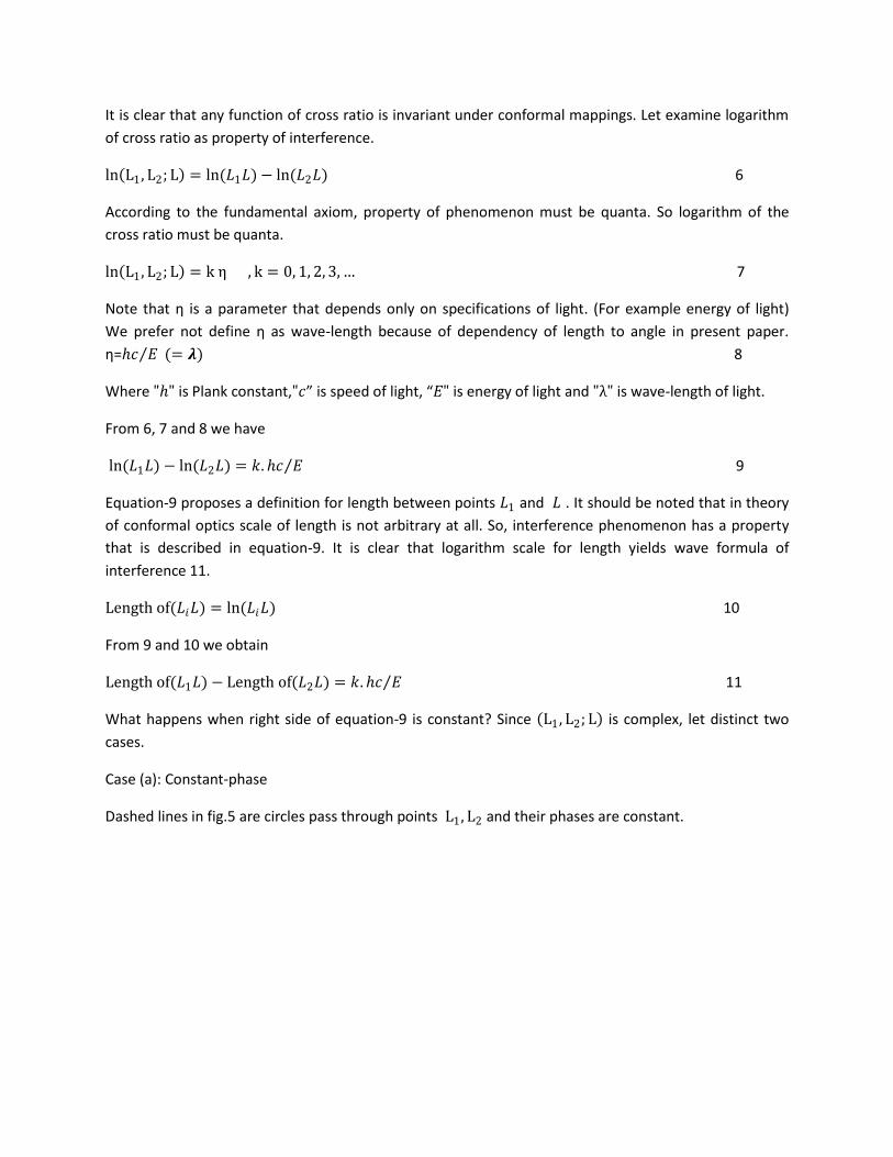
What happens when right side of equation-9 is constant? Since L1 , L2; L is complex, let distinct two

cases.

Case (a): Constant-phase

Dashed lines in fig.5 are circles pass through points L1 , L2 and their phases are constant.

s

L1

L

L2

Fig.5: Constant-phase diagram for L1 , L2; L

s

L1

L

L2

Fig.6: Constant-amplitude diagram for L1 , L2; L

Case (b): Constant-amplitude

Curved lines in fig.6 are circles that don’t intersect each other.

It should be noted that:

- Each dashed line in fig.5 is perpendicular to all curved lines of fig.6.

- Each curved line in fig.6 is perpendicular to all dashed lines of fig.5.

- Dashed lines in fig.5 may be considered as electric field or magnetic field and curved lines in fig.6

as position of Geiger counter. In present paper we do it.

- Dashed lines in fig.5 may be considered as possible paths between points L1 , L2 (for example

fluid flow in fluid mechanics) and curved lines in fig.6 as co-potential points.

Now let L1 move toward L2 in fig.6. We expect a descriptive diagram for diffraction phenomenon.

(fig.7)

s

L

=L1 L2

Fig.7: Descriptive diagram of diffraction phenomenon (for single slot)

For all points on curved lines in fig.7 L1 , L2; L is equal to zero. In other words for K = 0 in equation-9

all curved lines obtained.

Unfortunately quantum property of light is disappeared. So interference phenomenon does not lead us

to a quantitative theory of diffraction. A quantitative theory of diffraction will be presented in the next

section.

Section-5 (Diffraction phenomenon)

In this section a diffraction theory is extracted from the fundamental axiom of conformal optics. At first

we need to study conformal non-Euclidean models in the unit disk. (See appendix-2) According to the

fundamental axiom there is a property that remains unchanged under a conformal mapping from

diffraction scene to the unit disk. (fig.8)

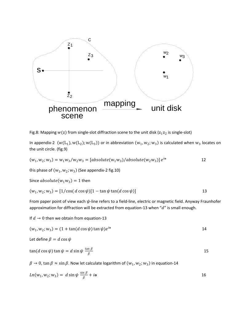
phenomenon unit disk

s

Z1

Z3

Z2

w1

w2w3

mapping

scene

C

Fig.8: Mapping 𝑤(z) from single-slot diffraction scene to the unit disk (z1z2 is single-slot)

In appendix-2 𝑤(L1), w(L2); w(L3 ) or in abbreviation w1 , w2; w3 is calculated when w3 locates on

the unit circle. (fig.9)

w1 , w2; w3 = w1w3 w2w3 = [𝑎𝑏𝑠𝑜𝑙𝑢𝑡𝑒(w1w3) 𝑎𝑏𝑠𝑜𝑙𝑢𝑡𝑒(w2w3)] 𝑒𝑖ɵ 12

ϴ is phase of w1 , w2; w3 (See appendix-2 fig.10)

Since 𝑎𝑏𝑠𝑜𝑙𝑢𝑡𝑒 w1w3 = 1 then

w1 , w2; w3 = [1 cos(𝑑 cos𝜓)[1 − tan𝜓 tan 𝑑 cos𝜓 ] 13

From paper point of view each 𝜓-line refers to a field-line, electric or magnetic field. Anyway Fraunhofer

approximation for diffraction will be extracted from equation-13 when “𝑑” is small enough.

If 𝑑 → 0 then we obtain from equation-13

w1 , w2; w3 = (1 + tan(𝑑 cos𝜓) tan𝜓)𝑒𝑖ɵ 14

Let define 𝛽 = 𝑑 cos𝜓

tan(𝑑 cos𝜓) tan𝜓 = 𝑑 sin𝜓 tan 𝛽

𝛽 15

𝛽 → 0, tan𝛽 ≈ sin𝛽. Now let calculate logarithm of w1 , w2; w3 in equation-14

𝐿𝑛 w1 , w2; w3 = 𝑑 sin𝜓 sin 𝛽

𝛽+ 𝑖ɵ 16

We need real part of equation-16 because Geiger counter measures real parameters. When you move

on a 𝜓-line real part of 𝐿𝑛 w1 , w2; w3 represents electric field.

𝑅𝑒𝑎𝑙[𝐸 w1 , w2; w3 ] = 𝑑tan 𝛽

𝛽 sin𝜓 = 𝐸 = 𝐸0 sin𝜓 17

For a period of oscillation we obtain from equation-17

𝐼 = 𝐸2 = 𝐸02 2 =

1

2(𝑑2𝑠𝑖𝑛𝑐2𝛽) 18

Equation-18 is the Fraunhofer approximation of diffraction phenomenon. Note that 𝑑2 2 should be

measured via Geiger counter as 𝐼0.

For large enough of “𝑑” diffraction model deviates from equation-18. It will be in general form as

follows:

I = [𝐿𝑛 1

cos 𝑑 cos 𝜓 [1−tan (𝑑 cos 𝜓) tan 𝜓)] ]2 19

The cross ratio and related diffraction should be defined for four points as follows:

w1 , w2; w3 , w4 =w1w3

w1w4

w2w4

w2w3=

1+tan (𝑑 cos 𝜓) tan 𝜓

1−tan (𝑑 cos 𝜓) tan 𝜓𝑒𝑖ɵ 20

I = {𝑅𝑒𝑎𝑙 𝐿𝑛 w1 , w2; w3 , w4 }2 = [𝐿𝑛

1+tan (𝑑 cos 𝜓) tan 𝜓

1−tan (𝑑 cos 𝜓) tan 𝜓]2 21

Now concentrate on equation-16. What is the meaning of imaginary part of logarithm? For many

reasons we have to define phase of 𝐿𝑛 w1 , w2; w3 as time. (See appendix-2, fig.10)

ϴ ≈ 𝑡 22

So when “𝑑” is small enough, 𝐿𝑛 w1 , w2; w3 should be represented as an interval of space-time in the

Minkowski diagram. In other words 𝐿𝑛 w1 , w2; w3 is an interval of space-time between events

w1 and w2. From this point of view we look at the unit disk as a space-time diagram. A space-time

diagram in the unit disk will be presented in other paper.

Section-6 (Conclusion)

We analyzed a variety of optical phenomena by use of just one axiom named fundamental axiom. Also a

bridge made between classic optics and conformal mapping via fundamental axiom. In appendix-1 cross

ratio for three points is defined mathematically. Although cross ratio should be developed for more than

three points we didn’t use developed form in present paper to hold simplicity. A theory of diffraction is

derived for single slot and it is shown that Fraunhofer equation of diffraction is obtained when slot is

small enough.

In appendix-2 a novel geometrical method is presented to understanding diffraction phenomenon. In

fact Poincare model in the unit disk is generalized to 𝜓 −models. Although we don’t pay any attention

these models are as beautiful as Poincare model. (For example triangle inequality is valid in 𝜓 −models)

In the end of section-5 we refer to Minkowski diagram. A novel representation of space-time in the unit

disk is predicted by the conformal optics. This space-time diagram must be locally in accordance with

the Minkowskian metric. (In fact it is done by author before and is presented in other paper)

Finally, conformal optics presents a geometrical approach to understanding optical phenomena.

Appendix-1 Cross ratio

In math, cross ratio for three points is defined by two ways as below

1-A

L1 , L2; L = L1L L2L

L1 , L2 and L , are three points in the complex (or projective) plane and don’t lie on a line.

2-A

L1 , L2; L = sin∠L1L sin∠L2L

L1 , L2 and L , are three lines in the complex (or projective) plane and intersect each other in unique

point.

These two different definitions show duality of points and lines in projective plane. The most important

property of cross ratio (or any function of cross ratio) is invariance under conformal mappings.

Cross ratio for four points is also defined by two ways as below:

1-B

w1 , w2; w3 , w4 =w1w3

w1w4

w2w4

w2w3

Where wi a point in the complex plane

2-B

w1 , w2; w3 , w4 =𝑠𝑖𝑛∠w1w3

sin∠w1w4 sin∠w2w4

𝑠𝑖𝑛∠w2w3

Where wi a line in the complex plane

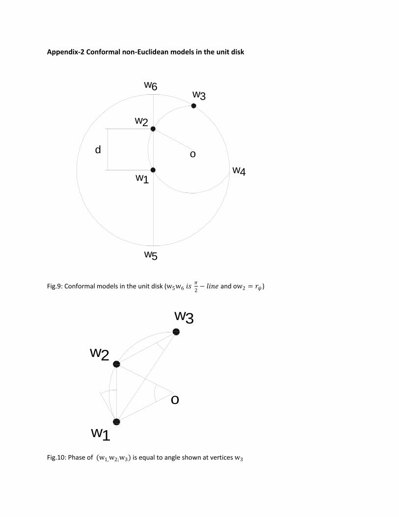
Appendix-2 Conformal non-Euclidean models in the unit disk

w1

w2

w3w6

w5

w4

d o

Fig.9: Conformal models in the unit disk (w5w6 𝑖𝑠 𝜋

2− 𝑙𝑖𝑛𝑒 and ow2 = 𝑟𝜓 )

w1

w2

w3

o

Fig.10: Phase of (w1,w2;w3) is equal to angle shown at vertices w3

In fig.9 two lines 𝜓 −line and 𝜋

2−line are shown. Note that

𝜋

2− 𝑙𝑖𝑛𝑒 known as Poincare-line. Each

𝜓 −line belongs to related 𝜓 −model and each 𝜓 −model represents related 𝜓 −geometry. So Poincare

model is a special case of a 𝜓 −model. In other words the hyperbolic geometry is special case of

𝜓 −geometry. Let define 𝜓 −model so that all its lines cut the unit circle at angle 𝜓. Without any

restriction suppose that 𝑤(𝑧) is determined by three points 𝑤1 ,𝑤2 𝑎𝑛𝑑 𝑤3 such that 𝑤1 is the center

of the unit disk. (See fig.9) Simple calculations yield:

𝑎𝑏𝑠𝑜𝑙𝑢𝑡𝑒 w1w3 = 𝑎𝑏𝑠𝑜𝑙𝑢𝑡𝑒 w1w6 = 𝑎𝑏𝑠𝑜𝑙𝑢𝑡𝑒 w1w5 = 𝑎𝑏𝑠𝑜𝑙𝑢𝑡𝑒 w1w4 = 1

𝑎𝑏𝑠𝑜𝑙𝑢𝑡𝑒 w2w3 = [1 − tan𝜓 tan 𝑑 cos𝜓 ] cos(𝑑 cos𝜓)

𝑎𝑏𝑠𝑜𝑙𝑢𝑡𝑒 w1w2 = 𝑑

𝑎𝑏𝑠𝑜𝑙𝑢𝑡𝑒 w2w5 = 1 + 𝑑

𝑎𝑏𝑠𝑜𝑙𝑢𝑡𝑒 w2w6 = 1 − 𝑑

𝑎𝑏𝑠𝑜𝑙𝑢𝑡𝑒 w2w4 = [1 + tan𝜓 tan 𝑑 cos𝜓 ] cos(𝑑 cos𝜓)

𝑎𝑏𝑠𝑜𝑙𝑢𝑡𝑒 w3w5 = 2 1 + sin(𝛳 + 𝜓)

𝑎𝑏𝑠𝑜𝑙𝑢𝑡𝑒 w3w6 = 2 1 − sin(𝛳 + 𝜓)

𝑎𝑏𝑠𝑜𝑙𝑢𝑡𝑒 w4w5 = 2 1 + sin(𝛳 − 𝜓)

𝑎𝑏𝑠𝑜𝑙𝑢𝑡𝑒 w4w6 = 2 1 − sin(𝛳 − 𝜓)

sin𝛳 = 𝑑 cos𝜓

𝑟𝜓 = 1 (2 cos𝜓)

We call “wiwj" cross functions of the unit disk. Cross function for three points or more than three points

can be calculated by these functions. From physical point of view these functions are important. For

example w2w3 leads us to the Fraunhofer approximation of diffraction phenomenon when

𝑎𝑏𝑠𝑜𝑙𝑢𝑡𝑒 w1w2 be small enough.