Introduction to Bayesian tracking

Doz. G. BleserProf. Stricker

Computer Vision: Object and People Tracking

• Goal:– Estimate posterior belief or state distribution based on control data 

and sensor measurements– Information represented as probability density function

• State: position of robot in corridor• Control data: odometry• Measurements: door sensors

2

Reminder: introductory example

Recursive Bayesian filtering

• Key idea 1: Probability distributions represent our belief about the state of the dynamical system

• Key idea 2:  Recursive cycle1. Predict from motion model2. Sensor measurement3. Correct the prediction

…repeat

predict

correct

measure

Outline

• Reminder: Basic concepts in probability• Terminology, notation, probabilistic laws• Bayes filters

4

Joint and Conditional Probability

• Let  and  denote two random variables:

,

• If  and  are independent (carry no information about each other) then:

p ,

5

Joint and Conditional Probability: example

• Ideal cube, dice toss: G={2, 4, 6}, A={4, 5, 6}

• ?

• ?

• , ?

• | ?

6

Joint and Conditional Probability: example

• Ideal cube, dice toss: G={2, 4, 6}, A={4, 5, 6}

•

•

• , 4,6

• | , 2 4,6

7

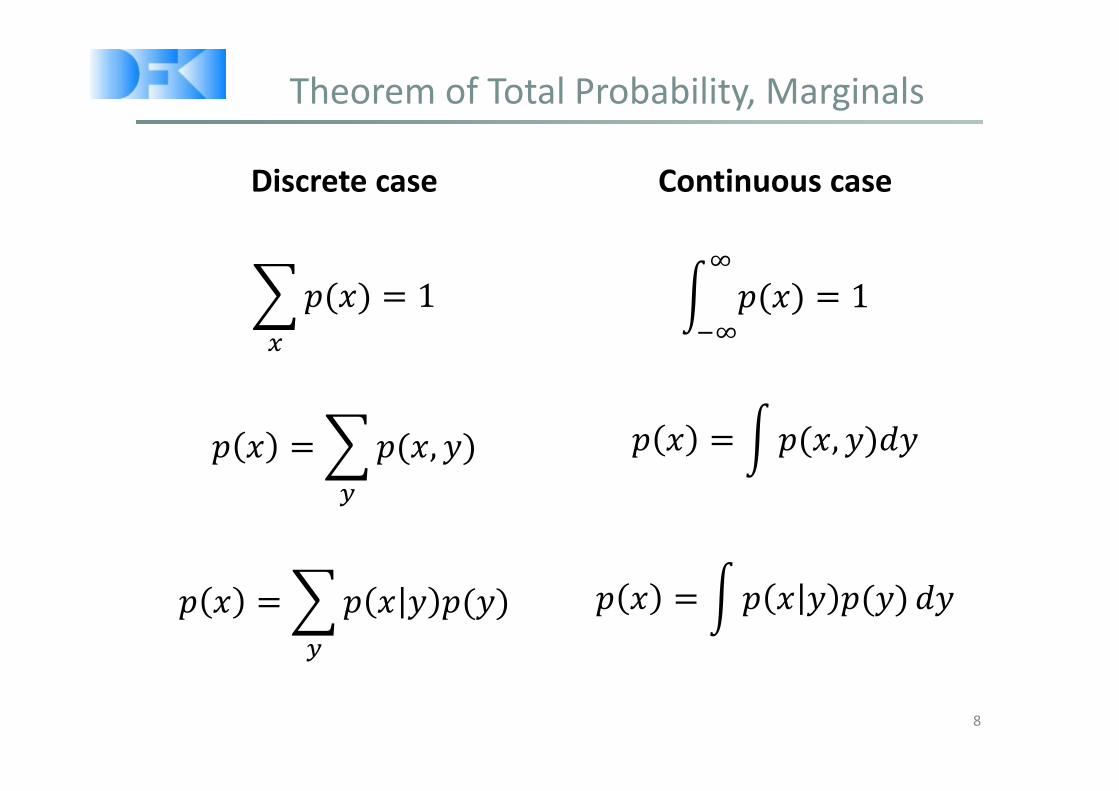
Theorem of Total Probability, Marginals

8

Discrete case Continuous case

Bayes Theorem

• In the context of state estimation:– Assume is a quantity that we want to infer from Think of  as state and  as sensor measurement

9

Posterior

probability

Generative model: how statevariables cause sensor

measurements

Independent of denoted as normalizer

Important: in this lecture, we will freely use  in different equations to 

denote normalizers, even if their actual values 

differ!

Conditional Independence

• All rules presented so far can be conditioned on an arbitrary random variable, e.g. Z

,, ||

, , |

• Conditional Independence:  and  are independent, given that  is known

,⇔ , , | ,

does not necessarily imply absolute independence10

carries no informationabout , if is known

SA-1

Towards the state estimation problem:terminology, notation, probabilistic laws

Terminology: overview

12

State Measurement model/likelihood

Motion model/transitionprobability

Inference

1tx tx1x 1tx Tx

tz1z 1tz 1tz Tz

State

• The environment or world is considered a dynamical system• The state contains all information that we want to know about the

system• Notation:  denotes the state at time • A state is called complete, if it is the best predictor for the future knowledge of past states, measurements, or controls carries noinformation about evolution of the state in the future

• Typical examples of states: – Object pose/velocity in global coordinate system continuous, 

dynamic– 3D positions of landmarks continuous, stationary– Whether a sensor is broken or not discrete, dynamic– Sensor biases discrete, stationary

13

Markov chain

State: examples

• Example for people tracking in 2D images 

14

t xx

x

( , )t x yx( , , )t x y hx

1 2{ , }t t tx x x

y

State: example

• Object defined by a point in an image– position– velocity– acceleration

Saad Ali and Mubarak Shah, Floor Fields for Tracking in High Density Crowd Scenes, European Conference on Computer Vision (ECCV), 2008.

( , )( , , , )( , , , , , )

t

t

t

x yx y x yx y x y x y

xxx

State: examples

16

• Camera/object pose(rotation, translation)

• Joint angles

Measurements

• Sensor measurements provide noisy (indirect) information about the state of the dynamical system under consideration

• Notation:– denotes a measurement at time – : denotes the set of all measurements acquired from time  to 

• Typical examples of sensor measurements:– Camera images (pixel‐/feature‐/object‐level)– Inertial measurements– GPS coordinates

17

Control inputs

• Control inputs carry noisy information about the change of thedynamic system under consideration

• Notation: – denotes control data at time – corresponds to the change of the state in time interval 1;– : , , … , denotes sequences of control data 

• Typical examples of control inputs:– Velocity: setting the velocity of a robot to 10 cm/s for the duration of 5 

seconds suggests that the robot is 50 cm ahead of its pose before– Odometry: odometers measure the revolution of wheels– No input (often the case in visual tracking)

18

State estimation example

• Dynamical system: tracking of billard balls by means of a cameralooking from above (without spin, collision, etc.)

• Pre‐requisite: camera pose known with respect to table

19Courtesy of U. Frese

State estimation example

• Dynamical system: tracking of billard balls by means of a cameralooking from above (without spin, collision, etc.)

• Pre‐requisite: camera pose known with respect to table• Which components are contained in:

– State  :– Measurement  : – Control input :

20Courtesy of U. Frese

State estimation example

• Dynamical system: tracking of billard balls by means of a cameralooking from above (without spin, collision, etc.)

• Pre‐requisite: camera pose known with respect to table• Which components are contained in (simple model):

– State  , , , [m]  position and velocity in reference frame of billard table

– Measurement  , [Pixel]  pixel position of ball in camera image

– Control input empty, however, we can assume constant velocity during a time interval

• Question: how could the Markov assumption be violated here?– E.g. badly calibrated camera– Interaction with other balls or table (collisions)– Physical aspects: spin, friction, …

21

Probabilistic generative laws

• The evolution of state and measurements is governed byprobabilistic laws

• State  is generated stochastically from state  :

: , : , :

• Assuming that the state is complete:

: , : , : ,

22

Markov assumption:

example of conditionalindependence

Probabilistic generative laws

• Measurement  is generated stochastically from state  :

: , : , :

• Assuming that the state is complete:

: , : , :

23

Another Markov assumption(conditional independence)

Odometry input u1: 1m forward.

Measurement z2: here is a door. 24

Introductory example

Probabilistic generative laws

25

• State transition probability– Specifies, how the state

evolves over time as a function of the previous stateand the current control data

• Measurement probability/likelihood– Specifies how measurements

are generated as function of thestate

– Measurements can beunderstood as noisy projectionsof the state

Dynamic Bayesian network/

Hidden Markov model

Motion 

model

Measurement 

modelThis is what we model!

Belief

• In Bayesian inference, we usually want to estimate the state given sequences of measurements  : and control data  : and the respective state transition  , and measurement probabilities 

• Our estimate of the true state is also called belief:

| : , :

| : , :

26

Posterior distribution of conditioned on all available data

after including the current measurement

Prediction of before including the currentmeasurement

Time update: calculationof predicted state fromcurrent state and control

input

Measurement update/correction: 

calculation of posteriorfrom predicted state

Odometry input u1: 1m forward.

Measurement z2: here is a door. 27

Introductory example

SA-1

A general algorithm for state estimation (inference): Bayes filter

Prediction

Correction

Prediction

Correction

Recursive Bayes filter algorithm

All entities are modelled as random variables with PDFs

Prediction

Correction

1 2 3

29

Recursive Bayesian filtering

• Use probability distributions to model the estimation problem– Prediction/time update: calculate prior belief based on dynamic model– Correction/measurement update: calculate posterior belief based on 

measurement model

30posterior likelihood motion model posterior at t-1

measure predictcorrect

2. Prediction 3. Measurement

1. Image acquisition 4. Modelmatching

5. Correction

Tracking pipeline

31

Recursive Bayes filter algorithm 

1. Bayes_filter( , , ):

2. for all do

3. = Time_update( , )

4. = Measurement_update( , )

5. endfor

6. return

32

Measurement update step derived

= Measurement_update( , )

: , :

, : , : : , :

: , :

: , :

33

Bayes

Markov, 

normalizer

Time update step derived

= Time_update( , )

: , :

, : , : : , :

, : , :

,

For a finite state space, the integral turns into a sum

34

Expand using

marginalization

Markov

Bayes update rule

35

Posteriorat time 

Posterior attime  1

State transition probabilityDynamic model

Measurement likelihoodMeasurement model

Bayes filter algorithm

Prerequisites:• Assumption: the world is Markov, i.e. the state is complete• Given: 3 probability density functions:

– Initial belief: – Measurement probability: – State transition probability:  ,

36

Hands‐on example of Bayesian inference

37

?

Prior belief

p staircase 0.1

Bayesian inference (measurement update)

p staircase| image p image |staircase p staircase

p im | stair p stair p im | nostair p nostair

0.7 0.1/ 0.7 0.1 0.2 0.9 0.28

Sensor model

p image| staircase 0.7p image| nostaircase 0.2

=

1. for all do

2. 3. endfor

38

Tip: how to calculate the normalization

)()|(1)(

)()|()(

)()|()(

1

xPxyPyP

xPxyPyP

xPxyPyxP

x

yx

xyx

yx

yxPx

xPxyPx

|

|

|

aux)|(:

aux1

)()|(aux:

Algorithm:The resulting 

distribution must integrate to 1

Summary: Bayes filter framework

• Given:– Stream of measurements  : and control data  : – Measurement model |– Dynamic model | ,– Prior/Initial probability of the system state 

• Wanted: – Estimate of the state  of a dynamical system– The posterior of the state is also called belief:bel

| : , :

39

Markov Assumption

Underlying Assumptions• Static world• Independent noise• Perfect model, no approximation errors

40

: : :: : :

Reality

Environment dynamics

Approximatecomputation

Sensor limitations

Random effects

Inaccuratemodels

41

Sources of errorand uncertainty

Summary: Bayes filters

• Probabilistic tool for recursively estimating the state of a dynamical system from noisy measurements and control inputs.

• Based on probabilistic concepts such as the Bayes theorem, marginalization, and conditional independence.

• Make a Markov assumption according to which the state is a complete summary of the past. In real‐world problems, thisassumption is usually an approximation!

• Can in the presented form only be implemented for simple estimation problems, requires either…or…– closed form solutions for multiplication and integral– restriction to finite state spaces

42

Outlook

• What is missing:– Concrete representations for belief– Concrete representations for probability density functions– Implementable and tractable filter approximations– Applicability to complex and continuous estimation problems– Hands‐on experience

• Readings:– Kalman Filtering book by Peter Maybeck, chapter 1: 

http://www.cs.unc.edu/~welch/kalman/maybeck.html• Next lectures:

– Filters: (Extended) Kalman filter– Measurement and motion models

43

Exercise 1

• Available at: http://av.dfki.de/images/stories/lectures/opt‐ss12/exercise1.pdf– Simple computations (probabilistic concepts, Bayes filter)– Handling of Gaussians (preparation for next lecture)

• If you want feedback, hand in solutions until June 12• Tutorial session: Thursday, 14.06.2012, 14:00‐15:30, DFKI, room 

2.04 (second floor)– Discussion of solutions– Preparation for next lecture (Bayes filter with Gaussians)

• Any questions?

44