Introduction to Bayesian Divergence Time Estimation
68
I B D T E Tracy Heath Ecology, Evolution, & Organismal Biology Iowa State University @trayc7 http://phyloworks.org SSB Workshop at Evolution 2015 Guarujá, Brazil
-
Upload
tracy-heath -
Category
Science
-
view
192 -
download
3
Transcript of Introduction to Bayesian Divergence Time Estimation
I BD TETracy Heath
Ecology, Evolution, & Organismal BiologyIowa State University
@trayc7http://phyloworks.org
SSB Workshop at Evolution 2015Guarujá, Brazil
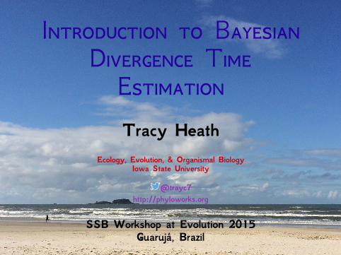
T-H MWhat I hope to emphasize here:• Bayes’ theorem is a beautiful thing• The substitution rate & time are confounded parameters• To estimate branch time we need separate models forthe rate along the branch & the time duration of thebranch
• Sequence data alone are not informative for absolutetime (in years)
• To infer absolute times, additional data (e.g., fossils orbiogeography) are needed
• It’s very important to have a good understanding of alldata (including fossils) used for divergence-timeestimation
Course materials: http://phyloworks.org/resources/evol2015ws.html
B I
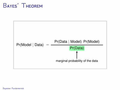
Estimate the probability of a hypothesis (model) conditionalon observed data.
The probability represents the researcher’s degree of belief.
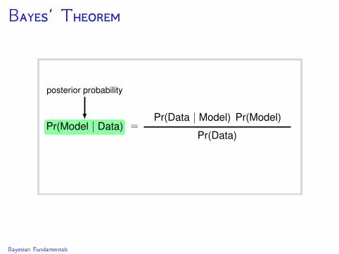
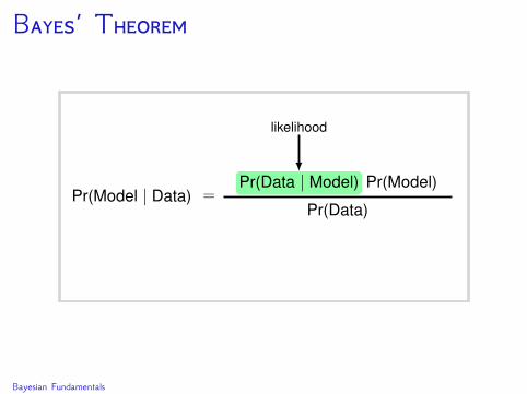
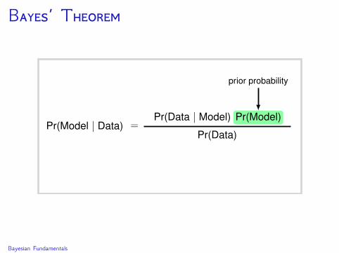
Bayes’ Theorem specifies the conditional probability of thehypothesis given the data.
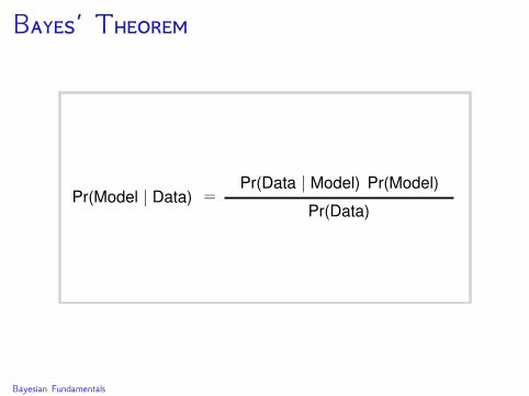
B’ T
Bayesian Fundamentals
B’ T
Bayesian Fundamentals
B’ T
Bayesian Fundamentals
B’ T
Bayesian Fundamentals
B’ T
Bayesian Fundamentals
B’ T
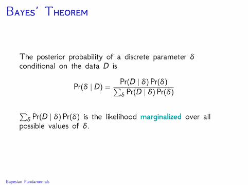
The posterior probability of a discrete parameter δconditional on the data D is
Pr(δ | D) =Pr(D | δ)Pr(δ)∑δ Pr(D | δ)Pr(δ)
∑δ Pr(D | δ)Pr(δ) is the likelihood marginalized over allpossible values of δ.
Bayesian Fundamentals
B’ T
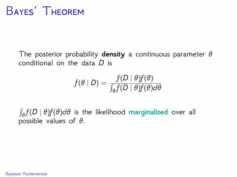
The posterior probability density a continuous parameter θconditional on the data D is
f(θ | D) =f(D | θ)f(θ)∫
θ f(D | θ)f(θ)dθ
∫θ f(D | θ)f(θ)dθ is the likelihood marginalized over allpossible values of θ.
Bayesian Fundamentals
E P P
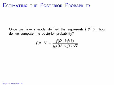
Once we have a model defined that represents f(θ | D), howdo we compute the posterior probability?
f(θ | D) =f(D | θ)f(θ)∫
θ f(D | θ)f(θ)dθ
Bayesian Fundamentals
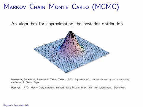
M C M C (MCMC)
An algorithm for approximating the posterior distribution
Metropolis, Rosenbluth, Rosenbluth, Teller, Teller. 1953. Equations of state calculations by fast computingmachines. J. Chem. Phys.
Hastings. 1970. Monte Carlo sampling methods using Markov chains and their applications. Biometrika.
Bayesian Fundamentals
M C M C (MCMC)
More on MCMC from Paul Lewis—our esteemed SSBPresident—and his lecture on Bayesian phylogenetics
Slides source: https://molevol.mbl.edu/index.php/Paul_Lewis
Bayesian Fundamentals
Paul O. Lewis (2014 Woods Hole Molecular Evolution Workshop) 42
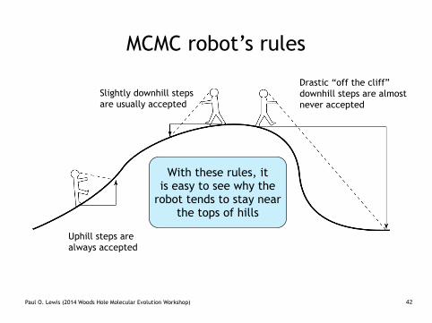
MCMC robot’s rules
Uphill steps are always accepted
Slightly downhill steps are usually accepted
Drastic “off the cliff” downhill steps are almost never accepted
With these rules, it is easy to see why the
robot tends to stay near the tops of hills
Paul O. Lewis (2014 Woods Hole Molecular Evolution Workshop) 43
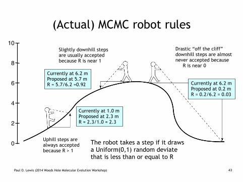
(Actual) MCMC robot rules
Uphill steps are always accepted because R > 1
Slightly downhill steps are usually accepted because R is near 1
Drastic “off the cliff” downhill steps are almost never accepted because R is near 0
Currently at 1.0 m Proposed at 2.3 m R = 2.3/1.0 = 2.3
Currently at 6.2 m Proposed at 5.7 m R = 5.7/6.2 =0.92 Currently at 6.2 m
Proposed at 0.2 m R = 0.2/6.2 = 0.03
6
8
4
2
0
10
The robot takes a step if it draws a Uniform(0,1) random deviate that is less than or equal to R
=
f(D|�⇤)f(�⇤)f(D)
f(D|�)f(�)f(D)
Paul O. Lewis (2014 Woods Hole Molecular Evolution Workshop) 44
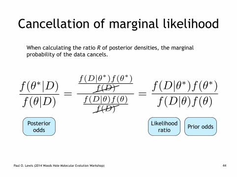
Cancellation of marginal likelihood
When calculating the ratio R of posterior densities, the marginal probability of the data cancels.
f(�⇤|D)
f(�|D)
Posterior odds
=f(D|�⇤)f(�⇤)f(D|�)f(�)
Likelihood ratio Prior odds
Paul O. Lewis (2014 Woods Hole Molecular Evolution Workshop) 45
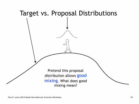
Target vs. Proposal Distributions
Pretend this proposal distribution allows good mixing. What does good
mixing mean?
default2.TXT
State0 2500 5000 7500 10000 12500 15000 17500
-10
-9
-8
-7
-6
-5
-4
-3
-2
-1
0
Paul O. Lewis (2014 Woods Hole Molecular Evolution Workshop) 46
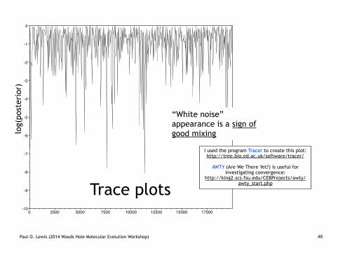
Trace plots
“White noise” appearance is a sign of good mixing
I used the program Tracer to create this plot: http://tree.bio.ed.ac.uk/software/tracer/ !
AWTY (Are We There Yet?) is useful for investigating convergence:
http://king2.scs.fsu.edu/CEBProjects/awty/awty_start.php
log(
post
erio
r)
Paul O. Lewis (2014 Woods Hole Molecular Evolution Workshop) 47
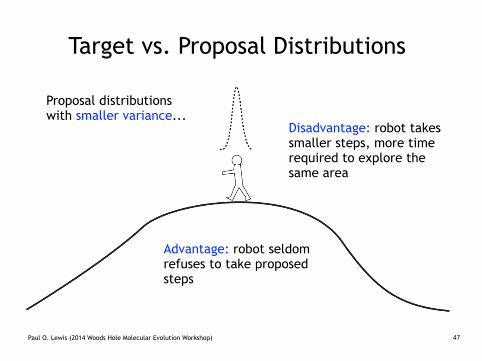
Target vs. Proposal Distributions
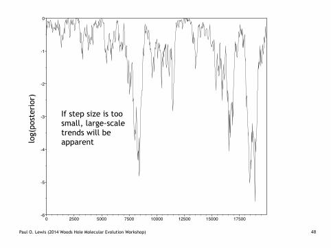
Proposal distributions with smaller variance...
Disadvantage: robot takes smaller steps, more time required to explore the same area
Advantage: robot seldom refuses to take proposed steps
smallsteps.TXT
State0 2500 5000 7500 10000 12500 15000 17500
-6
-5
-4
-3
-2
-1
0
Paul O. Lewis (2014 Woods Hole Molecular Evolution Workshop) 48
If step size is too small, large-scale trends will be apparentlo
g(po
ster
ior)
Paul O. Lewis (2014 Woods Hole Molecular Evolution Workshop) 49
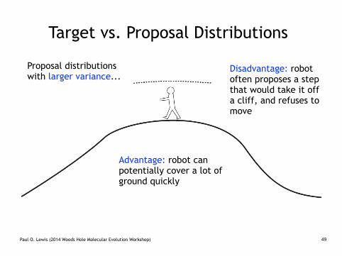
Target vs. Proposal Distributions
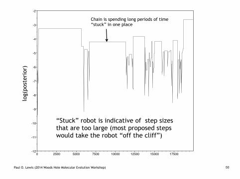
Proposal distributions with larger variance...
Disadvantage: robot often proposes a step that would take it off a cliff, and refuses to move
Advantage: robot can potentially cover a lot of ground quickly
bigsteps2.TX
T
State0 2500 5000 7500 10000 12500 15000 17500
-12
-11
-10
-9
-8
-7
-6
-5
-4
-3
-2
Paul O. Lewis (2014 Woods Hole Molecular Evolution Workshop) 50
Chain is spending long periods of time “stuck” in one place
“Stuck” robot is indicative of step sizes that are too large (most proposed steps would take the robot “off the cliff”)
log(
post
erio
r)
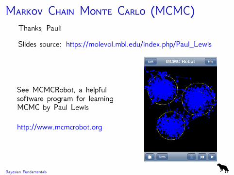
M C M C (MCMC)Thanks, Paul!
Slides source: https://molevol.mbl.edu/index.php/Paul_Lewis
See MCMCRobot, a helpfulsoftware program for learningMCMC by Paul Lewis
http://www.mcmcrobot.org
Bayesian Fundamentals
D T E
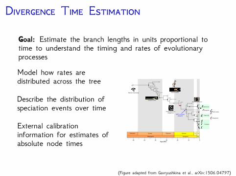
Goal: Estimate the branch lengths in units proportional totime to understand the timing and rates of evolutionaryprocesses
Model how rates aredistributed across the tree
Describe the distribution ofspeciation events over time
External calibrationinformation for estimates ofabsolute node times
Paleocene Eocene
102030405060 0
Oligocene Miocene Po Ps
Paleogene Neogene Qu.
Age (Ma)
MRCA of extant
penguins
Eudyptes
Megadyptes
Aptenodytes
Pygoscelis
Spheniscus
Eudyptula
Icadyptes salasi
Waimanu manneringi
Spheniscus muizoni
Palaeospheniscus
patagonicus
Kairuku waitaki
(Figure adapted from Gavryushkina et al., arXiv:1506.04797)
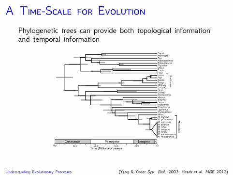
A T-S EPhylogenetic trees can provide both topological informationand temporal information
100 0.020.040.060.080.0
EquusRhinocerosBosHippopotamusBalaenopteraPhyseterUrsusCanisFelisHomoPanGorillaPongoMacacaCallithrixLorisGalagoDaubentoniaVareciaEulemurLemurHapalemurPropithecusLepilemur
MirzaM. murinusM. griseorufus
M. myoxinusM. berthaeM. rufus1M. tavaratraM. rufus2M. sambiranensisM. ravelobensis
Cheirogaleus
Sim
iiform
es
Mic
roce
bu
s
Cretaceous Paleogene Neogene Q
Time (Millions of years)
Understanding Evolutionary Processes (Yang & Yoder Syst. Biol. 2003; Heath et al. MBE 2012)
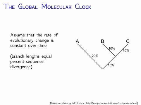
T G M C
Assume that the rate ofevolutionary change isconstant over time
(branch lengths equalpercent sequencedivergence) 10%
400 My
200 My
A B C
20%
10%10%
(Based on slides by Jeff Thorne; http://statgen.ncsu.edu/thorne/compmolevo.html)
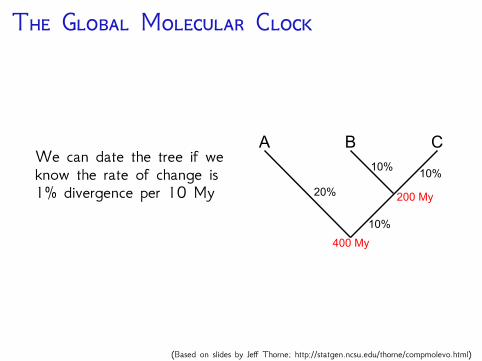
T G M C
We can date the tree if weknow the rate of change is1% divergence per 10 My N
A B C
20%
10%10%
10%200 My
400 My
200 My
(Based on slides by Jeff Thorne; http://statgen.ncsu.edu/thorne/compmolevo.html)
T G M C
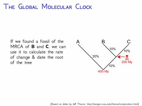
If we found a fossil of theMRCA of B and C, we canuse it to calculate the rateof change & date the rootof the tree
N
A B C
20%
10%10%
10%200 My
400 My
(Based on slides by Jeff Thorne; http://statgen.ncsu.edu/thorne/compmolevo.html)
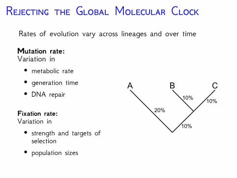
R G M CRates of evolution vary across lineages and over time
Mutation rate:Variation in• metabolic rate• generation time• DNA repair
Fixation rate:Variation in• strength and targets ofselection
• population sizes
10%
400 My
200 My
A B C
20%
10%10%
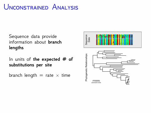
U A
Sequence data provideinformation about branchlengths
In units of the expected # ofsubstitutions per site
branch length = rate × time0.2 expected
substitutions/site
Phyl
ogen
etic
Rel
atio
nshi
psSe
quen
ceD
ata
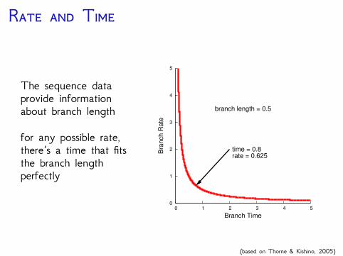
R T
The sequence dataprovide informationabout branch length
for any possible rate,there’s a time that fitsthe branch lengthperfectly
0
1
2
3
4
5
0 1 2 3 4 5
Bra
nch
Ra
te
Branch Time
time = 0.8rate = 0.625
branch length = 0.5
(based on Thorne & Kishino, 2005)
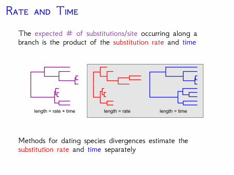
R TThe expected # of substitutions/site occurring along abranch is the product of the substitution rate and time
length = rate × time length = rate length = time
Methods for dating species divergences estimate thesubstitution rate and time separately
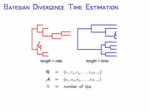
B D T E
length = rate length = time
R = (r, r, r, . . . , rN−)
A = (a, a, a, . . . , aN−)
N = number of tips
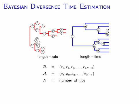
B D T E
length = rate length = time
R = (r, r, r, . . . , rN−)
A = (a, a, a, . . . , aN−)
N = number of tips
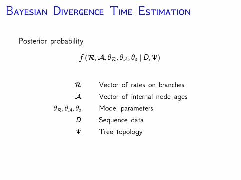
B D T E
Posterior probability
f (R,A, θR, θA, θs | D,Ψ)
R Vector of rates on branchesA Vector of internal node ages
θR, θA, θs Model parametersD Sequence dataΨ Tree topology
B D T E
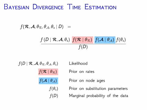
f(R,A, θR, θA, θs | D) =
f (D |R,A, θs) f(R | θR) f(A | θA) f(θs)f(D)
f(D |R,A, θR, θA, θs) Likelihoodf(R | θR) Prior on rates
f(A | θA) Prior on node agesf(θs) Prior on substitution parametersf(D) Marginal probability of the data
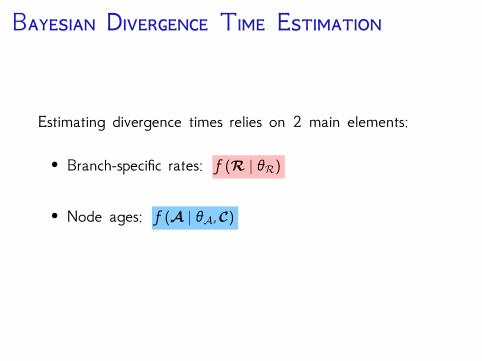
B D T E
Estimating divergence times relies on 2 main elements:
• Branch-specific rates: f (R | θR)
• Node ages: f (A | θA,C)
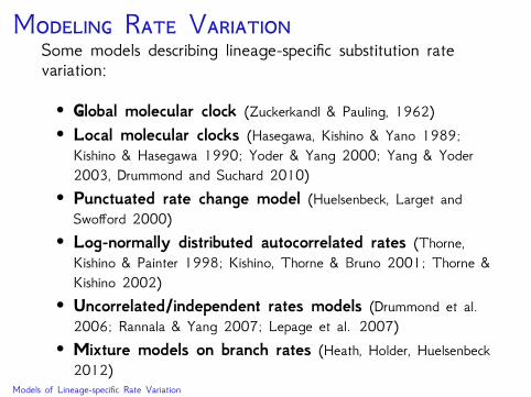
M R VSome models describing lineage-specific substitution ratevariation:
• Global molecular clock (Zuckerkandl & Pauling, 1962)• Local molecular clocks (Hasegawa, Kishino & Yano 1989;Kishino & Hasegawa 1990; Yoder & Yang 2000; Yang & Yoder2003, Drummond and Suchard 2010)
• Punctuated rate change model (Huelsenbeck, Larget andSwofford 2000)
• Log-normally distributed autocorrelated rates (Thorne,Kishino & Painter 1998; Kishino, Thorne & Bruno 2001; Thorne &Kishino 2002)
• Uncorrelated/independent rates models (Drummond et al.2006; Rannala & Yang 2007; Lepage et al. 2007)
• Mixture models on branch rates (Heath, Holder, Huelsenbeck2012)
Models of Lineage-specific Rate Variation
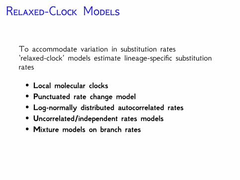
R-C M
To accommodate variation in substitution rates‘relaxed-clock’ models estimate lineage-specific substitutionrates
• Local molecular clocks• Punctuated rate change model• Log-normally distributed autocorrelated rates• Uncorrelated/independent rates models• Mixture models on branch rates
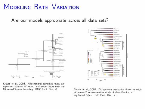
M R VAre our models appropriate across all data sets?
cave bear
American
black bear
sloth bear
Asian
black bear
brown bear
polar bear
American giant
short-faced bear
giant panda
sun bear
harbor seal
spectacled
bear
4.08
5.39
5.66
12.86
2.75
5.05
19.09
35.7
0.88
4.58
[3.11–5.27]
[4.26–7.34]
[9.77–16.58]
[3.9–6.48]
[0.66–1.17]
[4.2–6.86]
[2.1–3.57]
[14.38–24.79]
[3.51–5.89]14.32
[9.77–16.58]
95% CI
mean age (Ma)
t 2
t 3
t 4
t 6
t 7
t 5
t 8
t 9
t 10
t x
node
MP•MLu•MLp•Bayesian
100•100•100•1.00
100•100•100•1.00
85•93•93•1.00
76•94•97•1.00
99•97•94•1.00
100•100•100•1.00
100•100•100•1.00
100•100•100•1.00
t 1
Eocene Oligocene Miocene Plio Plei Hol
34 5.3 1.823.8 0.01
Epochs
Ma
Global expansion of C4 biomassMajor temperature drop and increasing seasonality
Faunal turnover
Krause et al., 2008. Mitochondrial genomes reveal anexplosive radiation of extinct and extant bears near theMiocene-Pliocene boundary. BMC Evol. Biol. 8.
Taxa
1
5
10
50
100
500
1000
5000
10000
20000
0100200300MYA
Ophidiiformes
Percomorpha
Beryciformes
Lampriformes
Zeiforms
Polymixiiformes
Percopsif. + Gadiif.
Aulopiformes
Myctophiformes
Argentiniformes
Stomiiformes
Osmeriformes
Galaxiiformes
Salmoniformes
Esociformes
Characiformes
Siluriformes
Gymnotiformes
Cypriniformes
Gonorynchiformes
Denticipidae
Clupeomorpha
Osteoglossomorpha
Elopomorpha
Holostei
Chondrostei
Polypteriformes
Clade r ε ΔAIC
1. 0.041 0.0017 25.32. 0.081 * 25.53. 0.067 0.37 45.1 4. 0 * 3.1Bg. 0.011 0.0011
Ostariophysi
Acanthomorpha
Teleo
stei
Santini et al., 2009. Did genome duplication drive the originof teleosts? A comparative study of diversification inray-finned fishes. BMC Evol. Biol. 9.
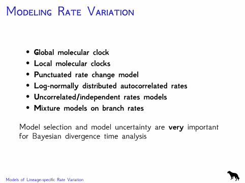
M R V
• Global molecular clock• Local molecular clocks• Punctuated rate change model• Log-normally distributed autocorrelated rates• Uncorrelated/independent rates models• Mixture models on branch rates
Model selection and model uncertainty are very importantfor Bayesian divergence time analysis
Models of Lineage-specific Rate Variation
B D T E
Estimating divergence times relies on 2 main elements:
• Branch-specific rates: f (R | θR)
• Node ages: f (A | θA,C)
http://bayesiancook.blogspot.com/2013/12/two-sides-of-same-coin.html
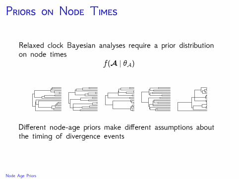
P N T
Relaxed clock Bayesian analyses require a prior distributionon node times
f(A | θA)
Different node-age priors make different assumptions aboutthe timing of divergence events
Node Age Priors
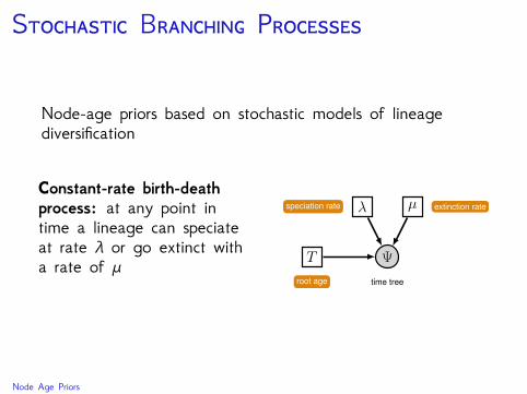
S B P
Node-age priors based on stochastic models of lineagediversification
Constant-rate birth-deathprocess: at any point intime a lineage can speciateat rate λ or go extinct witha rate of μ
Node Age Priors
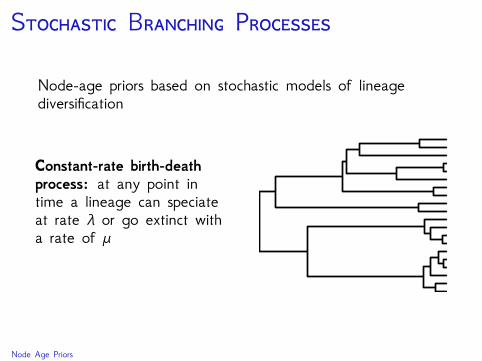
S B P
Node-age priors based on stochastic models of lineagediversification
Constant-rate birth-deathprocess: at any point intime a lineage can speciateat rate λ or go extinct witha rate of μ
Node Age Priors
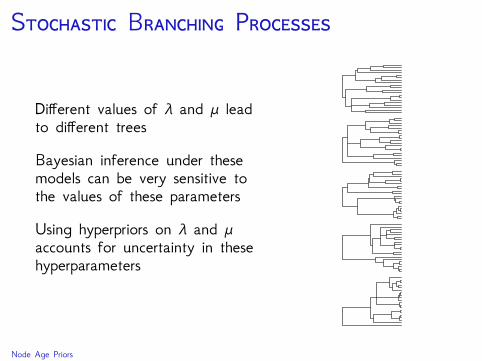
S B P
Different values of λ and μ leadto different trees
Bayesian inference under thesemodels can be very sensitive tothe values of these parameters
Using hyperpriors on λ and μaccounts for uncertainty in thesehyperparameters
Node Age Priors
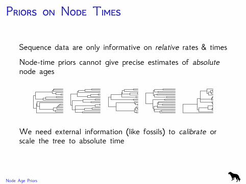
P N T
Sequence data are only informative on relative rates & timesNode-time priors cannot give precise estimates of absolutenode ages
We need external information (like fossils) to calibrate orscale the tree to absolute time
Node Age Priors
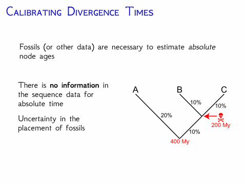
C D T
Fossils (or other data) are necessary to estimate absolutenode ages
There is no information inthe sequence data forabsolute timeUncertainty in theplacement of fossils
N
A B C
20%
10%10%
10%200 My
400 My
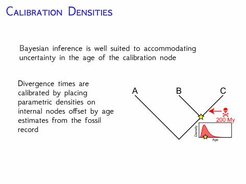
C D
Bayesian inference is well suited to accommodatinguncertainty in the age of the calibration node
Divergence times arecalibrated by placingparametric densities oninternal nodes offset by ageestimates from the fossilrecord
N
A B C
200 My
De
nsity
Age
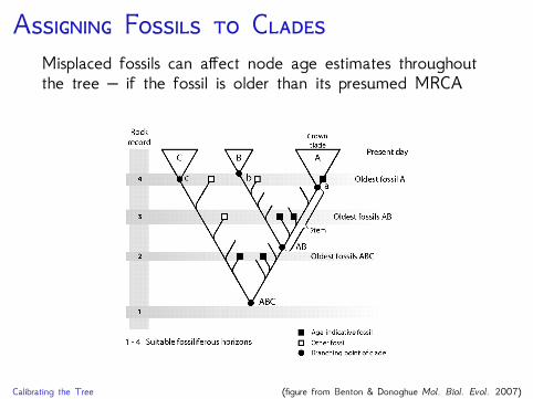
A F CMisplaced fossils can affect node age estimates throughoutthe tree – if the fossil is older than its presumed MRCA
Calibrating the Tree (figure from Benton & Donoghue Mol. Biol. Evol. 2007)
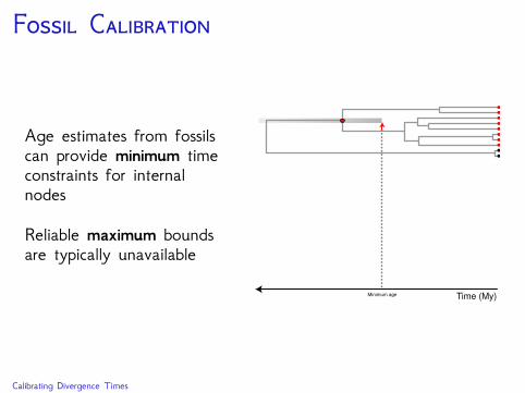
F C
Age estimates from fossilscan provide minimum timeconstraints for internalnodes
Reliable maximum boundsare typically unavailable
Minimum age Time (My)
Calibrating Divergence Times
P D C N
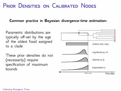
Common practice in Bayesian divergence-time estimation:
Parametric distributions aretypically off-set by the ageof the oldest fossil assignedto a clade
These prior densities do not(necessarily) requirespecification of maximumbounds
Uniform (min, max)
Exponential (λ)
Gamma (α, β)
Log Normal (µ, σ2)
Time (My)Minimum age
Calibrating Divergence Times
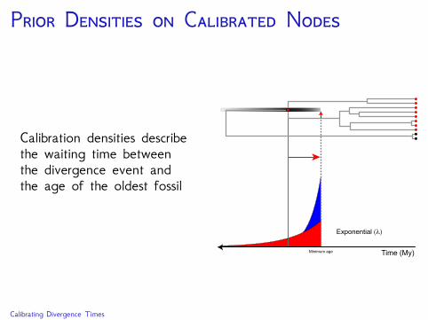
P D C N
Calibration densities describethe waiting time betweenthe divergence event andthe age of the oldest fossil
Minimum age
Exponential (λ)
Time (My)
Calibrating Divergence Times
P D C N
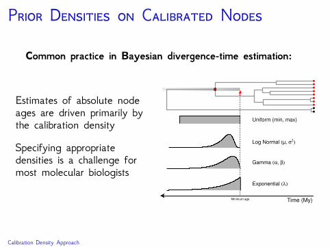
Common practice in Bayesian divergence-time estimation:
Estimates of absolute nodeages are driven primarily bythe calibration density
Specifying appropriatedensities is a challenge formost molecular biologists
Uniform (min, max)
Exponential (λ)
Gamma (α, β)
Log Normal (µ, σ2)
Time (My)Minimum age
Calibration Density Approach
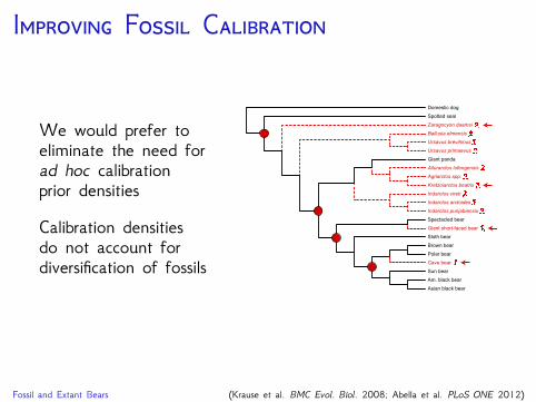
I F C
We would prefer toeliminate the need forad hoc calibrationprior densities
Calibration densitiesdo not account fordiversification of fossils
Domestic dog
Spotted seal
Giant panda
Spectacled bear
Sun bear
Am. black bear
Asian black bear
Brown bear
Polar bear
Sloth bear
Zaragocyon daamsi
Ballusia elmensis
Ursavus brevihinus
Ailurarctos lufengensis
Ursavus primaevus
Agriarctos spp.
Kretzoiarctos beatrix
Indarctos vireti
Indarctos arctoides
Indarctos punjabiensis
Giant short-faced bear
Cave bear
Fossil and Extant Bears (Krause et al. BMC Evol. Biol. 2008; Abella et al. PLoS ONE 2012)
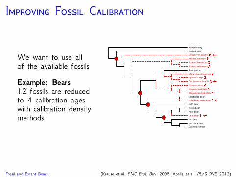
I F C
We want to use allof the available fossils
Example: Bears12 fossils are reducedto 4 calibration ageswith calibration densitymethods
Domestic dog
Spotted seal
Giant panda
Spectacled bear
Sun bear
Am. black bear
Asian black bear
Brown bear
Polar bear
Sloth bear
Zaragocyon daamsi
Ballusia elmensis
Ursavus brevihinus
Ailurarctos lufengensis
Ursavus primaevus
Agriarctos spp.
Kretzoiarctos beatrix
Indarctos vireti
Indarctos arctoides
Indarctos punjabiensis
Giant short-faced bear
Cave bear
Fossil and Extant Bears (Krause et al. BMC Evol. Biol. 2008; Abella et al. PLoS ONE 2012)
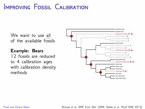
I F C
We want to use allof the available fossils
Example: Bears12 fossils are reducedto 4 calibration ageswith calibration densitymethods
Domestic dog
Spotted seal
Giant panda
Spectacled bear
Sun bear
Am. black bear
Asian black bear
Brown bear
Polar bear
Sloth bear
Zaragocyon daamsi
Ballusia elmensis
Ursavus brevihinus
Ailurarctos lufengensis
Ursavus primaevus
Agriarctos spp.
Kretzoiarctos beatrix
Indarctos vireti
Indarctos arctoides
Indarctos punjabiensis
Giant short-faced bear
Cave bear
Fossil and Extant Bears (Krause et al. BMC Evol. Biol. 2008; Abella et al. PLoS ONE 2012)
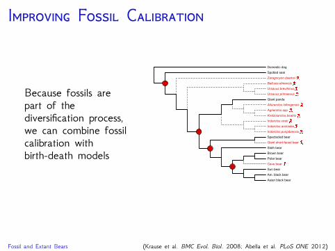
I F C
Because fossils arepart of thediversification process,we can combine fossilcalibration withbirth-death models
Domestic dog
Spotted seal
Giant panda
Spectacled bear
Sun bear
Am. black bear
Asian black bear
Brown bear
Polar bear
Sloth bear
Zaragocyon daamsi
Ballusia elmensis
Ursavus brevihinus
Ailurarctos lufengensis
Ursavus primaevus
Agriarctos spp.
Kretzoiarctos beatrix
Indarctos vireti
Indarctos arctoides
Indarctos punjabiensis
Giant short-faced bear
Cave bear
Fossil and Extant Bears (Krause et al. BMC Evol. Biol. 2008; Abella et al. PLoS ONE 2012)
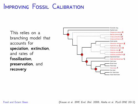
I F C
This relies on abranching model thataccounts forspeciation, extinction,and rates offossilization,preservation, andrecovery
Domestic dog
Spotted seal
Giant panda
Spectacled bear
Sun bear
Am. black bear
Asian black bear
Brown bear
Polar bear
Sloth bear
Zaragocyon daamsi
Ballusia elmensis
Ursavus brevihinus
Ailurarctos lufengensis
Ursavus primaevus
Agriarctos spp.
Kretzoiarctos beatrix
Indarctos vireti
Indarctos arctoides
Indarctos punjabiensis
Giant short-faced bear
Cave bear
Fossil and Extant Bears (Krause et al. BMC Evol. Biol. 2008; Abella et al. PLoS ONE 2012)

T F B-D P (FBD)
Improving statistical inference of absolute node ages
Eliminates the need to specify arbitrarycalibration densities
Better capture our statisticaluncertainty in species divergence dates
All reliable fossils associated with aclade are used
Useful for calibration or ‘total-evidence’dating
150 100 50 0
Time
(Heath, Huelsenbeck, Stadler. 2014 PNAS)
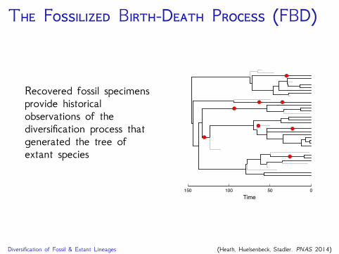
T F B-D P (FBD)
Recovered fossil specimensprovide historicalobservations of thediversification process thatgenerated the tree ofextant species
150 100 50 0
Time
Diversification of Fossil & Extant Lineages (Heath, Huelsenbeck, Stadler. PNAS 2014)
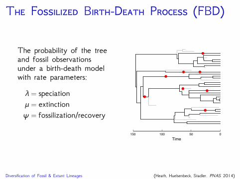
T F B-D P (FBD)
The probability of the treeand fossil observationsunder a birth-death modelwith rate parameters:
λ = speciationμ = extinctionψ = fossilization/recovery
150 100 50 0
Time
Diversification of Fossil & Extant Lineages (Heath, Huelsenbeck, Stadler. PNAS 2014)
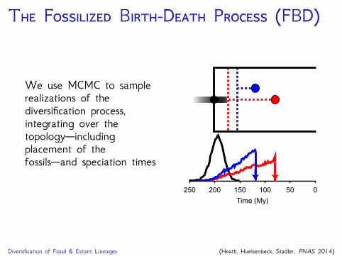
T F B-D P (FBD)
We use MCMC to samplerealizations of thediversification process,integrating over thetopology—includingplacement of thefossils—and speciation times
0250 50100150200
Time (My)
Diversification of Fossil & Extant Lineages (Heath, Huelsenbeck, Stadler. PNAS 2014)
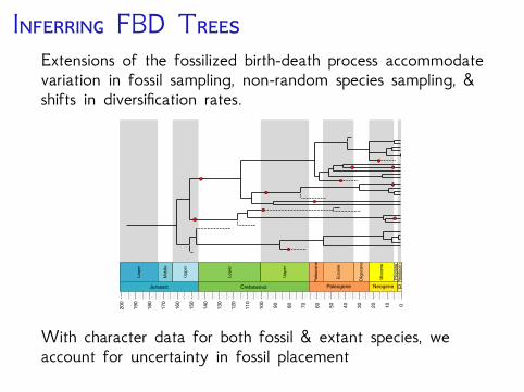
I FBD TExtensions of the fossilized birth-death process accommodatevariation in fossil sampling, non-random species sampling, &shifts in diversification rates.
0102030405060708090100
110
120
130
140
150
160
170
180
190
200
Lowe
r
Midd
le
Upper
Lowe
r
Upper
Paleo
cene
Eocene
Oligo
cene
Mioc
ene
Plioc
ene
Pleis
tocen
Jurassic Cretaceous Paleogene Neogene Q.
With character data for both fossil & extant species, weaccount for uncertainty in fossil placement
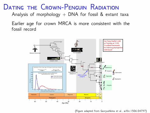
D C-P RAnalysis of morphology + DNA for fossil & extant taxaEarlier age for crown MRCA is more consistent with thefossil record
Paleocene Eocene
102030405060 0
Oligocene Miocene Po Ps
Paleogene Neogene Qu.
Age (Ma)
MRCA of extantpenguins
Eudyptes
Megadyptes
Aptenodytes
Pygoscelis
Spheniscus
Eudyptula
Icadyptes salasi
Waimanu manneringi
Spheniscus muizoni
Palaeospheniscuspatagonicus
Kairuku waitaki
See Tanja Stadler's talkon Tuesday at 13:30: “A uni�ed framework for inferring phylogenies with fossils''
(Figure adapted from Gavryushkina et al., arXiv:1506.04797)
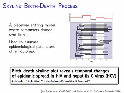
S B-D P
A piecewise shifting modelwhere parameters changeover timeUsed to estimateepidemiological parametersof an outbreak
0175 255075100125150
Days
(see Stadler et al. PNAS 2013 and Stadler et al. PLoS Currents Outbreaks 2014)
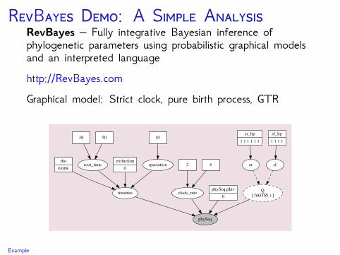
RB D: A S ARevBayes – Fully integrative Bayesian inference ofphylogenetic parameters using probabilistic graphical modelsand an interpreted languagehttp://RevBayes.comGraphical model: Strict clock, pure birth process, GTR
sf
Q[ fnGTR( ) ]
er_hp1 1 1 1 1 1
er
phySeq
sf_hp1 1 1 1
timetree
rho0.068
root_time
38 50
extinction0
speciation
10
clock_rate
2 4
phySeq.pInv0
Example
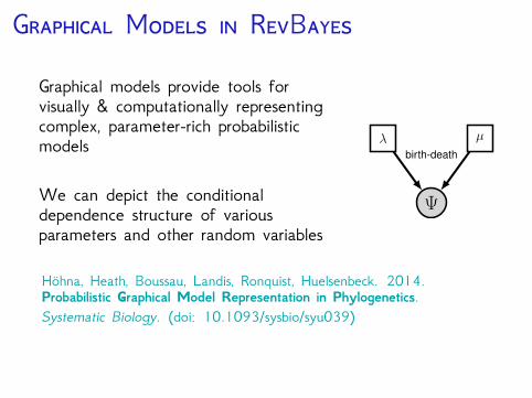
G M RB
Graphical models provide tools forvisually & computationally representingcomplex, parameter-rich probabilisticmodels
We can depict the conditionaldependence structure of variousparameters and other random variables
Höhna, Heath, Boussau, Landis, Ronquist, Huelsenbeck. 2014.Probabilistic Graphical Model Representation in Phylogenetics.Systematic Biology. (doi: 10.1093/sysbio/syu039)