MCB 137 VIRUS DYNAMICS WINTER 2008

1/10

VIRUS POPULATION DYNAMICS

Introduction: The basic epidemic model The classical model for epidemics is described in [1] and [Chapter 10 of 2].

Consider a population of uninfected individuals who wander randomly about a city. When they

encounter someone infected with a virus, there is a certain probability that they will become

infected. Infected people get sick for a while, then recover, where after they are immune to the

virus. We would like to construct a model the could predict the conditions for an epidemic to

break out.

There are three reservoirs of individuals:

S(t) = number of uninfected, but susceptible people at time t.

I(t) = number of infected people at time t.

R(t) = number of recovered people at time t.

The number of people in the city, N, is considered constant, S + I + R = N, at all times. Therefore

we can connect Flows between S and I, and between I and R. Call the Flow between S and I JSI =

InfectionRate, and the Flow between I and R JIR = RecoveryRate.1

SJ

SII

JIR

R

Now we must describe how the flows are controlled using Functions. First, what influences the

flow from S I? Suppose that the city is small and the people mill about at random in the town

square every day. Then encounters between susceptible and infected individuals occur at

random, and we can define an average infection rate by assuming random encounters similar to

that used in chemistry: S + I I ; that is, random collisions between uninfected and infected

individuals create new infections at a rate (with units [1/time], so that the flow between S and I

is:

JSI = S I.

Thus the InfectionRate flow depends on S, I, and , as shown by the arcs in Figure 1.

To model the flow from I to R, we assume that the average time an infected takes to recover is

1/a [1/days]. Thus the Flow between I and R is

JIR = a I,

where a is the rate constant (= the inverse of the mean lifetime in reservoir I).

The complete model is shown in Figure 1; all that is left is to assign numerical values to the

reservoir initial conditions and the two parameters, and a. In Figure 1 we have chosen to move

1 If the recovers lost their immunity and became susceptible to re-infection, then we would have to connect a flow

from R back to S; but we ignore this possibility here.

VIRUS DYNAMICS

2

the initial condition for the susceptibles outside the reservoir so that we can treat it as an

adjustable parameter, S0.

Figure 1. The basic epidemic model. (a) The reservoirs S, I, and R are the state variables. (b)

Since S + I + R = N, the reservoir R can be replaced by a Function: R = N S I.

Berkeley Madonna automatically keeps track of conserved flows, so this explicit

reduction is not strictly necessary for numerical calculations.

The Equation window gives the model equations can then be written directly in conventional

notation as follows: S Ia

R

Equation 1 dS

dt= SIInfectionrate

, S(0) = S0 Susceptible

Equation 2 dI

dt= SIInfectionrate

aIRecoveryrate

, I(0) =1 Infected

Equation 3 dR

dt= aIRecoveryrate

, R(0) = 0 Recovered

VIRUS DYNAMICS

3

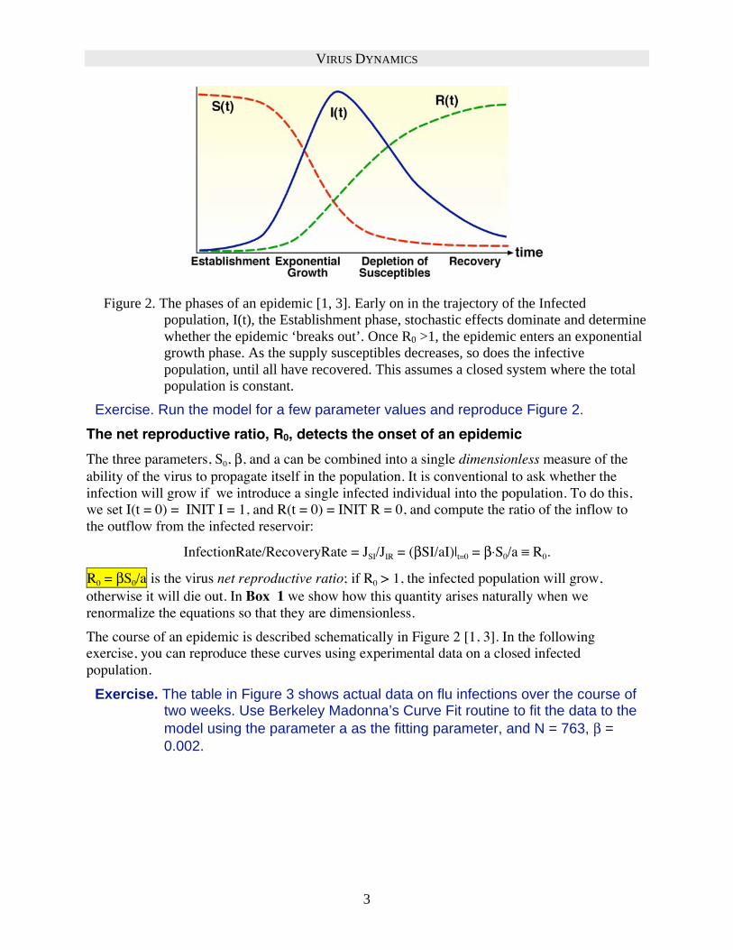
Figure 2. The phases of an epidemic [1, 3]. Early on in the trajectory of the Infected

population, I(t), the Establishment phase, stochastic effects dominate and determine

whether the epidemic ‘breaks out’. Once R0 >1, the epidemic enters an exponential

growth phase. As the supply susceptibles decreases, so does the infective

population, until all have recovered. This assumes a closed system where the total

population is constant.

Exercise. Run the model for a few parameter values and reproduce Figure 2.

The net reproductive ratio, R0, detects the onset of an epidemic

The three parameters, S0, , and a can be combined into a single dimensionless measure of the

ability of the virus to propagate itself in the population. It is conventional to ask whether the

infection will grow if we introduce a single infected individual into the population. To do this,

we set I(t = 0) = INIT I = 1, and R(t = 0) = INIT R = 0, and compute the ratio of the inflow to

the outflow from the infected reservoir:

InfectionRate/RecoveryRate = JSI/JIR = ( SI/aI)|t=0 = S0/a R0.

R0 = S0/a is the virus net reproductive ratio; if R0 > 1, the infected population will grow,

otherwise it will die out. In Box 1 we show how this quantity arises naturally when we

renormalize the equations so that they are dimensionless.

The course of an epidemic is described schematically in Figure 2 [1, 3]. In the following

exercise, you can reproduce these curves using experimental data on a closed infected

population.

Exercise. The table in Figure 3 shows actual data on flu infections over the course of two weeks. Use Berkeley Madonna’s Curve Fit routine to fit the data to the

model using the parameter a as the fitting parameter, and N = 763, =

0.002.

VIRUS DYNAMICS

4

Figure 3. Fitting the model to influenza data. The table gives the number of infecteds

measured over two weeks at a boys school. The outbreak began with a single

student from an initial population of 763. The infection rate, , was independently

estimated as = 0.00218.

Population dynamics of a virus in the body The demography of viruses inside a single organism is modeled very much like that of the

organisms themselves. In describing the basic model for virus dynamics we follow the treatment

Box 1. Setting the time scale defines R0

It is often a good idea to cast the equations the following form so that the various time scales can be

distinguished:

Equation 5 du

dt= ƒ(u, p),

where u is any of the reservoir variables, p represents the parameters and is the time constant.1 Since

we are most interested in the time scale of the infected population, we divide the equations by the

parameter a, so that the time constant for the infecteds is I = 1/a. Then the equations have the form

Equation 5

1

a

dS

dt=

aSI ,

1

a

dI

dt=

aS

0

Basic ReproductiveRatio

S

S0

I I ,1

a

dR

dt= I

It is sensible to measure time in units of I = 1/a; i.e. t t/a, and to measure the populations S and I as

a fraction of their initial value: S S/S0, I I/1. Of course, we cannot measure R this way since its

initial value is zero; however, since we know that R = N S I, R R/(N S0 1). If we substitute these

renormalized variables into Equation 5, we see that the dimensionless parameter R0 = S0/a controls

the dynamics of the system. This shows that the variable R is not really a variable since it can be

eliminated by using the conservation relation S + I + R = N. Therefore, we could replace the Reservoir

R by a Function. This is not necessary in Berkeley Madonna since the Flowchart automatically keeps

track of conserved flows.

Time[days] Infected 3 2.58E1

4 7.66E1

5 2.26E2

6 2.96E2

7 2.56E2

8 2.35E2

9 1.92E2

10 1.26E2

11 7.15E1

12 2.49E1

13 7.31E0 14 5.12E0

VIRUS DYNAMICS

5

found in Nowak and May’s classic text, which should be consulted for a more detailed treatment

[4].

The simplest model assumes that the body can be modeled as a ‘well stirred’ chemostat

containing the virus, V(t), and two kinds of cells: uninfected but susceptible cells, S(t), and cells

infected by virus, I(t). The life cycle of the virus is shown diagrammatically in Figure 4a.

Susceptible cells are produced by cell proliferation at a constant rate S0, live for an average

lifetime S = 1/ S, and die. Thus the deathrate of uninfected cells is their number divided by their

average lifetime S/ S. Virus infects cells to produce infected cells, I, with an ‘efficiency’, .

Since cells are infected by contact with virus, we model the infection rate as a simple mass action

reaction: S +V I . Infected cells die and release new viruses at a rate k; these viruses are

cleared from the system at rate c. Therefore, the model consists of three Reservoirs, denoted S, I,

and V.

Figure 4. (a) The virus life cycle. Susceptable cells (S) are supplied at a rate S0 and die at a

rate S = 1/ S. Virus (V) infects cells by a mass action rate: SV, where is the

efficiency of infection. Infected cells die at rate I; and release virus particles at rate

k. Viruses are cleared by the immune system at a rate c. (b) Flowchart for viral

dynamics.

The Flowchart shown in Figure 4b assigns reservoirs to the susceptible (S), infected (I) and virus

(V) compartments. The Flowchart produces the following set of equations in conventional

mathematical notation:

Equation 6 dS

dt= S0Supplyrate

SS

Deathrate

SVInfectionrate

Susceptible Cells

Equation 7 dI

dt= SVInfection

rate

II

Death

rate

Infected Cells

VIRUS DYNAMICS

6

Equation 8 dV

dt=

II

Virusproduction

cVVirus

clearance

Virus

The reproductive rate for a virus introduced into an uninfected population

We use the subscript ( )ss to denote steady state quantities. Before infection, V = I = 0, and the

steady state population of uninfected cells is given by Equation 6 when dS/dt = 0 = S0 S Sss, or

Sss = S0/ S. Let V0 = V(t = 0) be the number of viruses introduced at t = 0. The graph in Figure 5

shows the ‘impulse response’ of the system to the introduction of a single virus for the

parameters values shown in the figure.

Exercise: Make a slider to investigate the effect of varying the number of viruses

introduced at t = 0, and the virus amplification factor, . Find the value of

at which the virus becomes self-sustaining.

The rate of virus production (k) by one infected cell over its lifetime is called the ‘burst size’,

k/ . If the net virus production exceeds the rate at which they can be cleared from the system,

then the virus will ‘win’ in its competition with the immune system. So an important quantity

determining the outcome of this competition should be ratio [Production/Clearance]. In fact, we

can define a dimensionless ‘virus reproductive ratio’:

R0 = the number of infected cells generated by one uninfected cell (at the beginning of the

process, when there is not yet any infected cells) [1, 5]:

Equation 9

R0

S0

c

k

S I

Virus reproductive ratio

If R0 < 1, then the infection cannot establish itself because the virus does not infect cells as

rapidly as they are cleared from the system. This can be seen from the steady state solution to

equations 1-3 found by setting the rates dS/dt = dI/dt = dV/dt = 0 and solving for (Sss, Iss, Vss). A

bit of algebra shows that the steady state can be written as:

Equation 10 Sss=S0

R0

, Iss= R

01( ) I

c

k, V

ss= R

01( ) S

k Steady state

Since the steady state values must be positive, only when R0 > 1 can the virus establish itself.

Exercise. Make a parameter plot of the uninfected cells and virus as the infectivity, ,

increases. There is a sudden drop in the number of uninfected cells at a

critical value of ( Figure 6). Investigate this transition as and a vary to

show that the epidemic (as defined by a maximum in the infected cell population) occurs when R0 > 1.

VIRUS DYNAMICS

7

Figure 5. Population dynamics of susceptible cells (S), infected cells (I), and virus (V) when a

single virus is introduced into an uninfected population using the parameters given.

Figure 6. Long time cell and virus populations as the infectivity, , increases.

HIV chemotherapy model

Perelson, et al. formulated a simple model to describe the effect of an anti-viral drug on HIV

infected patients [6]. The model is shown in Figure 7a. Here the ‘target’ cells (T) for the drug are

modeled as a constant supply rate (e.g. from cell proliferation elsewhere), and the infected cells

are denoted by I. The target cell deathrate is , and each cell death releases N virus particles. The

corresponding flowchart is shown in Figure 7b, from which the equations describing the

populations of virus and infected cells are:

VIRUS DYNAMICS

8

Equation 11 dI

dt= VT

II, I(0) = 0 Infected cells

Equation 12 dV

dt= N

II cV , V (0) =V

0 Virus

where V0 is the initial viral load.

Exercise. Using the same parameters as the previous model, compute the steady state (Vss, Iss), and V(t) for various target cell populations, T.

Figure 7. The Perelson et al. model. (a) Target cells, T, are infected by virus, V, to produce

infected target cells T*

The antiviral drug inactivates the newly produced viruses, so that there are now two virus

populations: those still infective, VI,, and noninfective viruses, VNI, both of which are cleared at

the same rate, c.

Exercise. From the life cycle diagram in Figure 8a construct the Flowchart in Figure 8b, to obtain the population equations:

Equation 13. dI

dt= VT

II, I(0) = I

0 Infected target cells

Equation 14 dV

I

dt= cV

I, V

I(0) =V

0 Infective Virus

Equation 15 dV

NI

dt= N

II cV

NI, V

NI(0) = 0 Non-infective Virus

Because patients were treated with the viral drug at time t = 0, the initial condition for the

infected target cells must be set to the steady state value for the model with no drug (Equation

11, 7): I0 = kV0T/ .

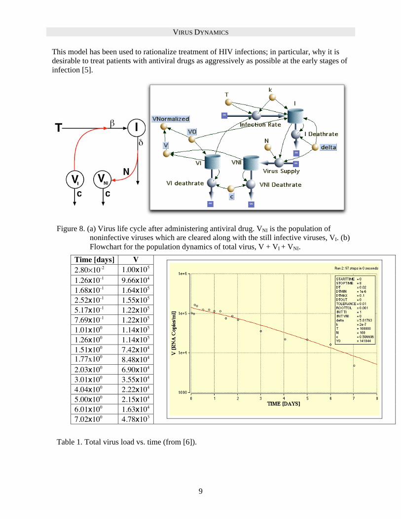
Exercise. Table 1 shows data taken from [6] giving the total viral load as a function of time

after administering an antiviral drug. Use Berkeley Madonna curve fitting

option to fit this data to the model, using as fitting parameters , c, and V0.

(The data can be loaded directly into Berkeley Madonna from a file.)

VIRUS DYNAMICS

9

This model has been used to rationalize treatment of HIV infections; in particular, why it is

desirable to treat patients with antiviral drugs as aggressively as possible at the early stages of

infection [5].

Figure 8. (a) Virus life cycle after administering antiviral drug. VNI is the population of

noninfective viruses which are cleared along with the still infective viruses, VI. (b)

Flowchart for the population dynamics of total virus, V + VI + VNI.

Time [days] V

2.80 10-2 1.00x105

1.26x10-1 9.66x104

1.68x10-1 1.64x105

2.52x10-1 1.55x105

5.17x10-1 1.22x105

7.69x10-1 1.22x105

1.01x100 1.14x105

1.26x100 1.14x105

1.51x100 7.42x104

1.77x100 8.48x104

2.03x100 6.90x104

3.01x100 3.55x104

4.04x100 2.22x104

5.00x100 2.15x104

6.01x100 1.63x104

7.02x100 4.78x103

Table 1. Total virus load vs. time (from [6]).

VIRUS DYNAMICS

10

References 1. Anderson, R. and R. May, Infectious Diseases of Humans. 1992, Oxford: Oxford

University Press.

2. Murray, J.D., Mathematical Biology. 3rd ed. Vol. 1, 2. 2002, New York: Springer.

3. Ferguson, N.M., M.J. Keeling, W.J. Edmunds, R. Gani, B.T. Grenfell5, R.M. Anderson,

and S. Leach, Planning for smallpox outbreaks. Nature, 2003. 425: p. 681 - 685.

4. May, R. and M. Nowak, Virus Dynamics: Mathematical Principles of Immunology and

Virology. 2001, Oxford: Oxford University Press. 256 pp.; 48 line illus.

5. Bonhoeffer, S., R.M. May, G.M. Shaw, and M.A. Nowak, Virus dynamics and drug

therapy. PNAS, 1997. 94: p. 6971-6976.

6. Perelson, A., A. Neumann, M. Markowitz, J. Leonard, and D. Ho, HIV-1 Dynamics in

Vivo: Virion Clearance Rate, Infected Cell Life-Span, and Viral Generation Time.

Science, 1996. 271: p. 1582-1586.