
Introduction - ackermath.info · 2 NILS ACKERMANN, MONICA CLAPP, AND ANGELA PISTOIA which blow-up...
25
BOUNDARY CLUSTERED LAYERS NEAR THE HIGHER CRITICAL EXPONENTS NILS ACKERMANN, M ´ ONICA CLAPP, AND ANGELA PISTOIA Abstract. We consider the supercritical problem -Δu = |u| p-2 u in Ω, u =0 on ∂Ω, where Ω is a bounded smooth domain in R N and p smaller than the crit- ical exponent 2 * N,k := 2(N-k) N-k-2 for the Sobolev embedding of H 1 (R N-k ) in L q (R N-k ), 1 ≤ k ≤ N - 3. We show that in some suitable domains Ω there are positive and sign changing solutions with positive and negative layers which concentrate along one or several k-dimensional submanifolds of ∂Ω as p ap- proaches 2 * N,k from below. Key words: Nonlinear elliptic boundary value problem; critical and su- percritical exponents; existence of positive and sign changing solutions. MSC2010: 35J60, 35J20. 1. Introduction Consider the classical Lane-Emden-Fowler problem (1) Δv + |v| p-2 v =0 in D, v =0 on ∂ D, where D is a bounded smooth domain in R N and p> 2. It is well known that when p is smaller than the critical Sobolev exponent 2 * := 2N N-2 , compactness of the Sobolev embedding ensures the existence of at least one positive solution and infinitely many sign changing solutions. In contrast, existence of solutions to problem (1) when p ≥ 2 * is a delicate issue. Pohozhaev’s identity [22] implies that problem (1) does not have a nontrivial solution if the domain D is strictly starshaped. On the other hand, Kazdan and Warner showed in [13] that if the domain D is an annulus, problem (1) has infinitely many radial solutions. For the critical case p =2 * Bahri and Coron [1] proved that a positive solution of (1) exists if the domain D has nontrivial reduced homology with Z/2-coefficients. Moreover, it was proved by Ge, Musso and Pistoia [11] and Musso and Pistoia [16] that, if D has a small hole, problem (1) has many sign changing solutions, whose number increases as the diameter of the hole decreases. Multiplicity results are also available for domains which are not small perturbations of a given domain, but have enough, possibly finite, symmetries, as proved by Clapp and Pacella [8] and Clapp and Faya [6]. The almost critical case p =2 * ± , with positive and small enough, has been widely studied. The slightly subcritical case p =2 * - was considered by Bahri, Li and Rey [2] and Rey [23], who showed the existence of positive solutions Date : October 2012. This research was partially supported by CONACYT grant 129847 and PAPIIT-DGAPA- UNAM grant IN106612 (Mexico), and by exchange funds of the Universit`a “La Sapienza” di Roma (Italy). 1
Transcript of Introduction - ackermath.info · 2 NILS ACKERMANN, MONICA CLAPP, AND ANGELA PISTOIA which blow-up...

BOUNDARY CLUSTERED LAYERS NEAR THE HIGHER
CRITICAL EXPONENTS
NILS ACKERMANN, MONICA CLAPP, AND ANGELA PISTOIA
Abstract. We consider the supercritical problem
−∆u = |u|p−2 u in Ω, u = 0 on ∂Ω,
where Ω is a bounded smooth domain in RN and p smaller than the crit-
ical exponent 2∗N,k :=2(N−k)N−k−2
for the Sobolev embedding of H1(RN−k) in
Lq(RN−k), 1 ≤ k ≤ N − 3. We show that in some suitable domains Ω there
are positive and sign changing solutions with positive and negative layers whichconcentrate along one or several k-dimensional submanifolds of ∂Ω as p ap-
proaches 2∗N,k from below.
Key words: Nonlinear elliptic boundary value problem; critical and su-
percritical exponents; existence of positive and sign changing solutions.
MSC2010: 35J60, 35J20.
1. Introduction
Consider the classical Lane-Emden-Fowler problem
(1) ∆v + |v|p−2v = 0 in D, v = 0 on ∂D,where D is a bounded smooth domain in RN and p > 2.
It is well known that when p is smaller than the critical Sobolev exponent 2∗ :=2NN−2 , compactness of the Sobolev embedding ensures the existence of at least onepositive solution and infinitely many sign changing solutions. In contrast, existenceof solutions to problem (1) when p ≥ 2∗ is a delicate issue. Pohozhaev’s identity [22]implies that problem (1) does not have a nontrivial solution if the domain D isstrictly starshaped. On the other hand, Kazdan and Warner showed in [13] that ifthe domain D is an annulus, problem (1) has infinitely many radial solutions.
For the critical case p = 2∗ Bahri and Coron [1] proved that a positive solutionof (1) exists if the domain D has nontrivial reduced homology with Z/2-coefficients.Moreover, it was proved by Ge, Musso and Pistoia [11] and Musso and Pistoia [16]that, if D has a small hole, problem (1) has many sign changing solutions, whosenumber increases as the diameter of the hole decreases. Multiplicity results arealso available for domains which are not small perturbations of a given domain, buthave enough, possibly finite, symmetries, as proved by Clapp and Pacella [8] andClapp and Faya [6].
The almost critical case p = 2∗ ± ε, with ε positive and small enough, hasbeen widely studied. The slightly subcritical case p = 2∗ − ε was considered byBahri, Li and Rey [2] and Rey [23], who showed the existence of positive solutions
Date: October 2012.This research was partially supported by CONACYT grant 129847 and PAPIIT-DGAPA-
UNAM grant IN106612 (Mexico), and by exchange funds of the Universita “La Sapienza” di
Roma (Italy).1

2 NILS ACKERMANN, MONICA CLAPP, AND ANGELA PISTOIA
which blow-up at one or more points of D as ε → 0. A large number of signchanging solutions with simple or multiple positive and negative blow-up pointswere constructed by Bartsch, Micheletti and Pistoia [3], Musso and Pistoia [17],and Pistoia and Weth [21]. For the slightly supercritical case p = 2∗ + ε existenceand nonexistence of positive solutions with one or more blow-up points has beenestablished by Ben Ayed, El Mehdi, Grossi and Rey [9], Pistoia and Rey [20], anddel Pino, Felmer and Musso [5].
Unlike the critical case, in the supercritical case p > 2∗ the existence of a non-trivial homology class in D does not guarantee the existence of a nontrivial solutionto (1). In fact, for each integer k such that 1 ≤ k ≤ N − 3, Passaseo [18, 19]exhibited a bounded smooth domain in RN , homotopically equivalent to the k-dimensional sphere, in which problem (1) does not have a nontrivial solution for
p ≥ 2∗N,k := 2(N−k)N−k−2 . Note that 2∗N,k is the critical Sobolev exponent in dimension
N − k. Examples of domains with richer homology were recently given by Clapp,Faya and Pistoia [7], where it was shown that for p > 2∗N,k there are bounded
smooth domains in RN whose cup-length is k + 1, in which problem (1) does nothave a nontrivial solution. On the other hand, for p = 2∗N,k existence of infinitely
many solutions in some domains has been recently established by Wei and Yan [25].Further multiplicity results may be found in [7].
In [10] del Pino, Musso and Pacard considered the case p = 2∗N,1 − ε and provedthat for some suitable domains D, if ε is positive, small enough and different froman explicit set of values, problem (1) has a positive solution which concentratesalong a 1-dimensional submanifold of the boundary ∂D. In the same paper, theauthors ask the question whether one can find solutions which concentrate at ak-dimensional submanifold for p slightly below 2∗N,k. More precisely, they ask thefollowing:
Problem 1.1. Given 1 ≤ k ≤ N − 3, are there domains D in which problem (1)has a positive solution vp for each p < 2∗N,k with the property that these solutionsconcentrate along a k-dimensional submanifold of the boundary ∂D as p→ 2∗N,k?
Having in mind that when p approaches the first critical exponent 2∗ from belowa large number of sign changing solutions exist, another question arises naturally:
Problem 1.2. Given 1 ≤ k ≤ N−3, are there domains D in which problem (1) hasa sign changing solution vp for each p < 2∗N,k with the property that these solutionsconcentrate along a k-dimensional submanifold of the boundary ∂D as p→ 2∗N,k?
In this paper, we give a positive answer to both questions. In particular, foreach set of positive integers k1, . . . , km with k := k1 + · · ·+ km ≤ N − 3 we exhibitdomains D in which problem (1) has a positive solution for each p < 2∗N,k and,as p → 2∗N,k, these solutions concentrate along a k-dimensional submanifold M of
the boundary ∂D which is diffeomorphic to the product of spheres Sk1 × · · · × Skm .Moreover, problem (1) has also a sign changing solution with a positive and anegative layer, both of which concentrate along M as p→ 2∗N,k. This follows fromour main results, which we next state.
Fix k1, . . . , km ∈ N with k := k1 + · · · + km ≤ N − 3 and a bounded smoothdomain Ω in RN−k such that
(2) Ω ⊂ (x1, . . . , xm, x′) ∈ Rm × RN−k−m : xi > 0, i = 1, . . . ,m.

BOUNDARY CLUSTERED LAYERS NEAR THE HIGHER CRITICAL EXPONENTS 3
Set(3)D := (y1, . . . , ym, z) ∈ Rk1+1 × · · · × Rkm+1 × RN−k−m :
(∣∣y1∣∣ , . . . , |ym| , z) ∈ Ω.
D is a bounded smooth domain in RN which is invariant under the action of thegroup Γ := O(k1 + 1)× · · · ×O(km + 1) on RN given by
(g1, . . . , gm)(y1, . . . , ym, z) := (g1y1, . . . , gmy
m, z).
for every gi ∈ O(ki+1), yi ∈ Rki+1, z ∈ RN−k−m. Here, as usual, O(d) denotes thegroup of all linear isometries of Rd. For p = 2∗N,k − ε we shall look for Γ-invariant
solutions to problem (1), i.e. solutions v of the form
(4) v(y1, . . . , ym, z) = u(∣∣y1∣∣ , . . . , |ym| , z).
A simple calculation shows that v solves problem (1) if and only if u solves
−∆u−m∑i=1
kixi
∂u
∂xi= |u|p−2u in Ω, u = 0 on ∂Ω.
This problem can be rewritten as
−div(a(x)∇u) = a(x)|u|p−2u in Ω, u = 0 on ∂Ω,
where a(x1, . . . , xN−k) := xk11 · · ·xkmm . Note that 2∗N,k is the critical exponent indimension n := N − k which is the dimension of Ω.
Thus, we are lead to study the more general almost critical problem
(5) −div(a(x)∇u) = a(x) |u|4
n−2−ε u in Ω, u = 0 on ∂Ω,
where Ω is a bounded smooth domain in Rn, n ≥ 3, ε is a positive parameter, anda ∈ C2(Ω) is strictly positive on Ω.
This is a subcritical problem, so standard variational methods yield one positiveand infinitely many sign changing solutions to problem (5) for every ε ∈ (0, 4
n−2 ),
cf. Proposition 4.1 in [7]. Our goal is to construct solutions uε with positive andnegative bubbles which accumulate at some points ξ1, . . . , ξκ of ∂Ω as ε→ 0. Theycorrespond, via (4), to Γ-invariant solutions vε of problem (1) with positive andnegative layers which accumulate along the k-dimensional submanifolds
Mj := (y1, . . . , ym, z) ∈ Rk1+1×· · ·×Rkm+1×RN−k−m :(∣∣y1
∣∣ , . . . , |ym| , z) = ξj
of the boundary of D as ε→ 0. Note that each Mj is diffeomorphic to Sk1×· · ·×Skmwhere Sd is the unit sphere in Rd+1.
We will assume one of the following conditions.
(a1) There exist κ nondegenerate critical points ξ1, . . . , ξκ ∈ ∂Ω of the restrictionof a to ∂Ω such that
〈∇a(ξi), ν(ξi)〉 > 0 ∀i = 1, . . . , κ,
where ν(ξi) is the inward pointing unit normal to ∂Ω at ξi.(a2) There exists a critical point ξ0 ∈ ∂Ω of the restriction of a to ∂Ω such
that 〈∇a(ξ0), ν(ξ0)〉 > 0, and vectors τ1, . . . , τn−1 ∈ Rn such that the setν(ξ0), τ1, . . . , τn−1 is orthonormal and Ω and a are invariant with respectto the reflection %i on each of the hyperplanes ξ0 + τi = 0, i.e.
%i(x) ∈ Ω and a(%i(x)) = a(x) ∀x ∈ Ω,
4 NILS ACKERMANN, MONICA CLAPP, AND ANGELA PISTOIA
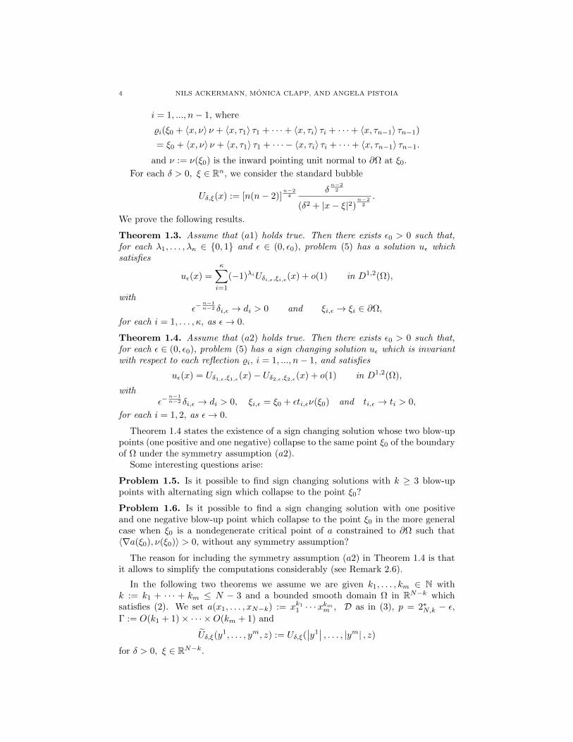
i = 1, ..., n− 1, where
%i(ξ0 + 〈x, ν〉 ν + 〈x, τ1〉 τ1 + · · ·+ 〈x, τi〉 τi + · · ·+ 〈x, τn−1〉 τn−1)
= ξ0 + 〈x, ν〉 ν + 〈x, τ1〉 τ1 + · · · − 〈x, τi〉 τi + · · ·+ 〈x, τn−1〉 τn−1.
and ν := ν(ξ0) is the inward pointing unit normal to ∂Ω at ξ0.
For each δ > 0, ξ ∈ Rn, we consider the standard bubble
Uδ,ξ(x) := [n(n− 2)]n−24
δn−22
(δ2 + |x− ξ|2)n−22
.
We prove the following results.
Theorem 1.3. Assume that (a1) holds true. Then there exists ε0 > 0 such that,for each λ1, . . . , λκ ∈ 0, 1 and ε ∈ (0, ε0), problem (5) has a solution uε whichsatisfies
uε(x) =
κ∑i=1
(−1)λiUδi,ε,ξi,ε(x) + o(1) in D1,2(Ω),
withε−
n−1n−2 δi,ε → di > 0 and ξi,ε → ξi ∈ ∂Ω,
for each i = 1, . . . , κ, as ε→ 0.
Theorem 1.4. Assume that (a2) holds true. Then there exists ε0 > 0 such that,for each ε ∈ (0, ε0), problem (5) has a sign changing solution uε which is invariantwith respect to each reflection %i, i = 1, ..., n− 1, and satisfies
uε(x) = Uδ1,ε,ξ1,ε(x)− Uδ2,ε,ξ2,ε(x) + o(1) in D1,2(Ω),
withε−
n−1n−2 δi,ε → di > 0, ξi,ε = ξ0 + εti,εν(ξ0) and ti,ε → ti > 0,
for each i = 1, 2, as ε→ 0.
Theorem 1.4 states the existence of a sign changing solution whose two blow-uppoints (one positive and one negative) collapse to the same point ξ0 of the boundaryof Ω under the symmetry assumption (a2).
Some interesting questions arise:
Problem 1.5. Is it possible to find sign changing solutions with k ≥ 3 blow-uppoints with alternating sign which collapse to the point ξ0?
Problem 1.6. Is it possible to find a sign changing solution with one positiveand one negative blow-up point which collapse to the point ξ0 in the more generalcase when ξ0 is a nondegenerate critical point of a constrained to ∂Ω such that〈∇a(ξ0), ν(ξ0)〉 > 0, without any symmetry assumption?
The reason for including the symmetry assumption (a2) in Theorem 1.4 is thatit allows to simplify the computations considerably (see Remark 2.6).
In the following two theorems we assume we are given k1, . . . , km ∈ N withk := k1 + · · · + km ≤ N − 3 and a bounded smooth domain Ω in RN−k whichsatisfies (2). We set a(x1, . . . , xN−k) := xk11 · · ·xkmm , D as in (3), p = 2∗N,k − ε,Γ := O(k1 + 1)× · · · ×O(km + 1) and
Uδ,ξ(y1, . . . , ym, z) := Uδ,ξ(
∣∣y1∣∣ , . . . , |ym| , z)
for δ > 0, ξ ∈ RN−k.

BOUNDARY CLUSTERED LAYERS NEAR THE HIGHER CRITICAL EXPONENTS 5
Theorem 1.7. Assume that (a1) holds true for a and Ω as above. Then thereexists ε0 > 0 such that, for each λ1, . . . , λκ ∈ 0, 1 and ε ∈ (0, ε0), problem (1) hasa Γ-invariant solution vε which satisfies
vε(x) =
κ∑i=1
(−1)λiUδi,ε,ξi,ε(x) + o(1) in D1,2(D),
withε−
n−1n−2 δi,ε → di > 0 and ξi,ε → ξi ∈ ∂Ω,
for each i = 1, . . . , κ, as ε→ 0.
Theorem 1.8. Assume that (a2) holds true for a and Ω as above. Then thereexists ε0 > 0 such that, for each ε ∈ (0, ε0), problem (1) has a Γ-invariant signchanging solution vε which satisfies
vε(x) = Uδ1,ε,ξ1,ε(x)− Uδ2,ε,ξ2,ε(x) + o(1) in D1,2(D),
withε−
n−1n−2 δi,ε → di > 0, ξi,ε = ξ0 + εti,εν(ξ0) and ti,ε → ti > 0,
for each i = 1, 2, as ε→ 0.
By the previous discussion Theorems 1.7 and 1.8 follow immediately from The-orems 1.3 and 1.4. The proof of Theorems 1.3 and 1.4 relies on a very well knownLjapunov-Schmidt reduction procedure. We shall omit many details on this proce-dure because they can be found, up to some minor modifications, in the literature.We only compute what cannot be deduced from known results.
The outline of the paper is as follows: In Section 2 we write the approximatesolution, sketch the Ljapunov-Schmidt procedure and use it to prove Theorems 1.3and 1.4. In Appendix B we compute the rate of the error term and in Appendix Cwe estimate the reduced energy. In Appendix A we give some important estimateson the Green function close to the boundary.
2. The variational setting
We take
(u, v) :=
∫Ω
a(x)∇u · ∇v dx, ‖u‖ :=
(∫Ω
a(x) |∇u|2 dx)1/2
,
as the inner product in H10(Ω) and its corresponding norm. Since a is strictly
positive and bounded in Ω they are well defined and equivalent to the standardones. Similarly, for each r ∈ [1,∞),
‖u‖r :=
(∫Ω
a(x) |u|r dx)1/r
is a norm in Lr(Ω) which is equivalent to the standard one.
Next, we rewrite problem (5) in a different way. Let i∗ : L2nn+2 (Ω) → H1
0(Ω) be
the adjoint operator to the embedding i : H10(Ω) → L
2nn−2 (Ω), i.e. i∗(u) = v if and
only if
(v, ϕ) =
∫Ω
a(x)u(x)ϕ(x)dx for all ϕ ∈ C∞c (Ω)
if and only if
− div(a(x)∇v) = a(x)u in Ω, v = 0 on ∂Ω.

6 NILS ACKERMANN, MONICA CLAPP, AND ANGELA PISTOIA
Clearly, there exists a positive constant c such that
‖i∗(u)‖ ≤ c ‖u‖ 2nn+2
∀ u ∈ L2nn+2 (Ω).
Setting p := 2nn−2 and fε(s) := |s|p−2−ε
s, problem (5) turns out to be equivalent to
(6) u = i∗ (fε(u)) , u ∈ H10(Ω).
Set f(s) := f0(s) and αn := [n(n− 2)]n−24 . Let
Uδ,ξ := αnδn−22
(δ2 + |x− ξ|2)n−22
, δ > 0, ξ ∈ Rn,
be the positive solutions to the limit problem
−∆u = f(u), u ∈ H1(Rn).
Set
ψ0δ,ξ(x) :=
∂Uδ,ξ∂δ
= αnn− 2
2δn−42
|x− ξ|2 − δ2
(δ2 + |x− ξ|2)n/2
and, for each j = 1, . . . , n,
ψjδ,ξ(x) :=∂Uδ,ξ∂ξj
= αn(n− 2)δn−22
xj − ξj(δ2 + |x− ξ|2)n/2
.
Recall that the space spanned by the (n + 1) functions ψjδ,ξ is the set of solutionsto the linearized problem
−∆ψ = (p− 1)Up−2δ,ξ ψ in Rn.
Let PW denote the projection of the function W ∈ D1,2(Rn) onto H10(Ω), i.e.
∆PW = ∆W in Ω, PW = 0 on ∂Ω.
We look for two different types of solutions to problem (5). The solutions foundin Theorem 1.3 are of the form
(7) uε =
κ∑i=1
(−1)λiPUδi,ε,ξi,ε + φ,
for fixed λi ∈ 0, 1, where the concentration parameters satisfy
(8) δi,ε = εn−1n−2 di for some di > 0,
and the concentration points satisfy
(9) ξi,ε = si + ηiν(si) where si ∈ ∂Ω and ηi = εti for some ti > 0.
Here and in the following ν(si) denotes the inward unit normal to the boundary∂Ω at the point si.
On the other hand, the solutions found in Theorem 1.4 are of the form
(10) uε =∑i=1
(−1)i+1PUδi,ε,ξi,ε + φ,
where the concentration parameters satisfy (8), while the concentration points arealigned on the line L := ξ0 + rν(ξ0) : r ∈ R, namely
(11) ξi,ε = ξ0 + ηiν(ξ0) where ηi = εti for some 0 < t1 < · · · < t`.
BOUNDARY CLUSTERED LAYERS NEAR THE HIGHER CRITICAL EXPONENTS 7
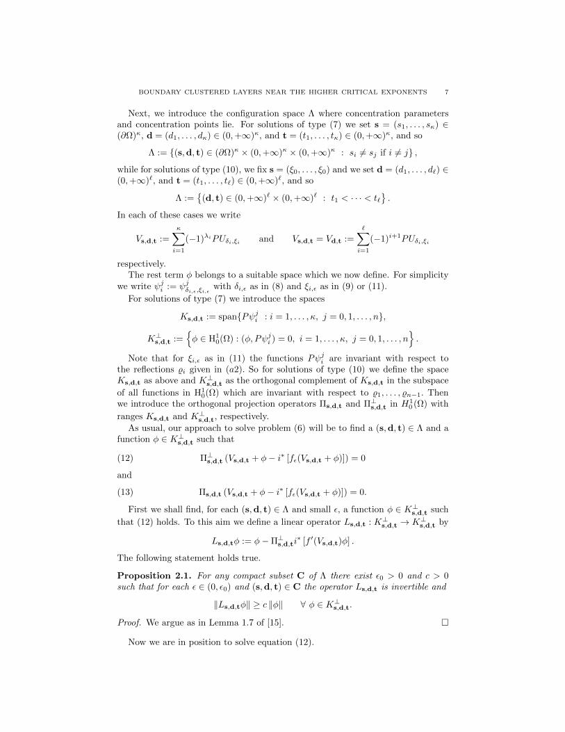
Next, we introduce the configuration space Λ where concentration parametersand concentration points lie. For solutions of type (7) we set s = (s1, . . . , sκ) ∈(∂Ω)κ, d = (d1, . . . , dκ) ∈ (0,+∞)κ, and t = (t1, . . . , tκ) ∈ (0,+∞)κ, and so
Λ := (s,d, t) ∈ (∂Ω)κ × (0,+∞)κ × (0,+∞)κ : si 6= sj if i 6= j ,
while for solutions of type (10), we fix s = (ξ0, . . . , ξ0) and we set d = (d1, . . . , d`) ∈(0,+∞)`, and t = (t1, . . . , t`) ∈ (0,+∞)`, and so
Λ :=
(d, t) ∈ (0,+∞)` × (0,+∞)` : t1 < · · · < t`.
In each of these cases we write
Vs,d,t :=
κ∑i=1
(−1)λiPUδi,ξi and Vs,d,t = Vd,t :=∑i=1
(−1)i+1PUδi,ξi
respectively.The rest term φ belongs to a suitable space which we now define. For simplicity
we write ψji := ψjδi,ε,ξi,ε with δi,ε as in (8) and ξi,ε as in (9) or (11).
For solutions of type (7) we introduce the spaces
Ks,d,t := spanPψji : i = 1, . . . , κ, j = 0, 1, . . . , n,
K⊥s,d,t :=φ ∈ H1
0(Ω) : (φ, Pψji ) = 0, i = 1, . . . , κ, j = 0, 1, . . . , n.
Note that for ξi,ε as in (11) the functions Pψji are invariant with respect tothe reflections %i given in (a2). So for solutions of type (10) we define the spaceKs,d,t as above and K⊥s,d,t as the orthogonal complement of Ks,d,t in the subspace
of all functions in H10(Ω) which are invariant with respect to %1, . . . , %n−1. Then
we introduce the orthogonal projection operators Πs,d,t and Π⊥s,d,t in H10 (Ω) with
ranges Ks,d,t and K⊥s,d,t, respectively.
As usual, our approach to solve problem (6) will be to find a (s,d, t) ∈ Λ and afunction φ ∈ K⊥s,d,t such that
(12) Π⊥s,d,t (Vs,d,t + φ− i∗ [fε(Vs,d,t + φ)]) = 0
and
(13) Πs,d,t (Vs,d,t + φ− i∗ [fε(Vs,d,t + φ)]) = 0.
First we shall find, for each (s,d, t) ∈ Λ and small ε, a function φ ∈ K⊥s,d,t such
that (12) holds. To this aim we define a linear operator Ls,d,t : K⊥s,d,t → K⊥s,d,t by
Ls,d,tφ := φ−Π⊥s,d,ti∗ [f ′(Vs,d,t)φ] .
The following statement holds true.
Proposition 2.1. For any compact subset C of Λ there exist ε0 > 0 and c > 0such that for each ε ∈ (0, ε0) and (s,d, t) ∈ C the operator Ls,d,t is invertible and
‖Ls,d,tφ‖ ≥ c ‖φ‖ ∀ φ ∈ K⊥s,d,t.
Proof. We argue as in Lemma 1.7 of [15].
Now we are in position to solve equation (12).

8 NILS ACKERMANN, MONICA CLAPP, AND ANGELA PISTOIA
Proposition 2.2. For any compact subset C of Λ there exist ε0, c, σ > 0 such thatfor each ε ∈ (0, ε0) and (s,d, t) ∈ C there exists a unique φεs,d,t ∈ K⊥s,d,t such that
(12) holds and
(14)∥∥φεs,d,t∥∥ ≤ cε 1
2 +σ.
Proof. We estimate the rate of the error term
(15) Rs,d,t := Π⊥s,d,t (Vs,d,t − i∗ [fε(Vs,d,t)])
in Appendix B. Then we argue exactly as in Proposition 2.3 of [3].
The critical points of the energy functional Jε : H10(Ω)→ R defined by
Jε(u) :=1
2
∫Ω
a(x)|∇u|2dx− 1
p− ε
∫Ω
a(x)|u|p−εdx
are the solutions to problem (5). We define the reduced energy functional Jε : Λ→R by
Jε(s,d, t) := Jε(Vs,d,t + φεs,d,t)
The critical points of Jε are the solutions to problem (13).
Proposition 2.3. The function Vs,d,t + φεs,d,t is a critical point of the functional
Jε if and only if the point (s,d, t) is a critical point of the function Jε.
Proof. We argue as in Proposition 1 of [2].
The problem is thus reduced to the search for critical points of Jε, so it is
necessary to compute the asymptotic expansion of Jε.
Proposition 2.4. In case (7) it holds true that
Jε(s,d, t) = (c1 + c2ε log ε)
κ∑i=1
a(si)
(16)
+ ε
κ∑i=1
[c3a(si) + c4〈∇a(si), ν(si)〉ti + c5a(si)
(di2ti
)n−2
− c6a(si) log di
]+ o(ε),
C1-uniformly on compact sets of Λ. Here the ci’s are constants and c4, c5, c6 arepositive.
Proof. The proof is postponed to Appendix C.
Proposition 2.5. In case (10) it holds true that
(17) Jε(s,d, t) = Jε(d, t) = a(ξ0) [c1 + c2ε log ε+ c3ε] + εΨ(d, t) + o(ε),

BOUNDARY CLUSTERED LAYERS NEAR THE HIGHER CRITICAL EXPONENTS 9
C0-uniformly on compact sets of Λ. Here
(18) Ψ(d, t) := c4〈∇a(ξ0), ν(ξ0)〉∑i=1
ti + c5a(ξ0)×
×
∑i=1
(di2ti
)n−2
+∑i,j=1i6=j
(−1)i+j+1(didj)n−22
[1
|ti − tj |n−2− 1
|ti + tj |n−2
]
− c6a(ξ0)∑i=1
log di
where the ci’s are constants and c4, c5, c6 are positive.
Proof. The proof is postponed to Appendix C.
Proof of Theorem 1.3. Firstly, by Proposition 2.4, we get
Jε(s,d, t) = (c1 + c2ε log ε)
κ∑i=1
a(si) +O(ε),
C1-uniformly on compact sets of Λ. Then, since ξ1, . . . , ξκ are non degenerate criticalpoints of a constrained to the boundary of Ω, if ε is small enough there exist
sε := (s1,ε, . . . , sκ,ε) such that each si,ε → ξi as ε goes to zero, and∇sJε(sε,d, t) = 0.Secondly, by Proposition 2.4, we also get
Jε(sε,d, t)− (c1 + c2ε log ε)
κ∑i=1
a(si,ε)
= ε
κ∑i=1
[c3a(si,ε) + c4〈∇a(si,ε), ν(si,ε)〉ti
+ c5a(si,ε)
(di2ti
)n−2
− c6a(si,ε) log di
]+ o(ε)
= ε
κ∑i=1
[c3a(ξi) + c4〈∇a(ξi), ν(ξi)〉ti
+ c5a(ξi)
(di2ti
)n−2
− c6a(ξi) log di
]+ o(ε).
It is easy to verify that the function
(d, t)→κ∑i=1
[c4〈∇a(ξi), ν(ξi)〉ti + c5a(ξi)
(di2ti
)n−2
− c6a(ξi) log di
]
has a minimum point which is stable under C0-perturbations. Therefore, there
exists a point (dε, tε) such that ∇(d,t)Jε(sε,dε, tε) = 0. Thus, the function Jε hasa critical point and the claim follows from Proposition 2.3.

10 NILS ACKERMANN, MONICA CLAPP, AND ANGELA PISTOIA
Proof of Theorem 1.4. In this case ` = 2 and function Ψ defined in (18) reduces to
Ψ(d, t) = c4〈a(ξ0), ν(ξ0)〉(t1 + t2)
+ c5a(ξ0)
(d1
2t1
)n−2
+
(d2
2t2
)n−2
+ 2(d1d2)n−22
[1
|ti − tj |n−2− 1
|ti + tj |n−2
]− c6a(ξ0)(log d1 + log d2).
It is easy to verify that it has minimum point which is stable under C0-perturbations. Therefore, from Proposition 2.5 we deduce that, if ε is small enough,
the function Jε has a critical point. Now the claim follows from Proposition 2.3.
Remark 2.6. The symmetry assumption (a2) allows to overcome some technicaldifficulties which arise when looking for a solution whose bubbles collapse to thesame point. Indeed, the problem arises when we study the reduced energy and wehave to compute the contribution of each peak and the interaction among the peaks.The contribution of each peak is clear: it is given by the distance from the peakto the boundary as in (64) and by the value of the function a at the projectionof the peak onto the boundary as in (58). On the other hand, to compute theinteraction among the peaks (see (65)) it is important to compare the geodesicdistance d(si, sj) between the projections of the peaks onto the boundary with thedistance |ηiν(si)− ηjν(sj)| between the normal components of the peaks. To havea good expansion the distance d(si, sj) should be negligible with respect to thedistance |ηiν(si)− ηjν(sj)|. But then, in order to find a criticality in the points si,we need to go further in the expansion and computations become too tedious. Ifthe domain Ω and the function a are symmetric, we can overcome this difficultyjust by assuming that the peaks satisfy (11), so that d(si, sj) = 0. In this case theinteraction among the peaks is clear and it is given in terms of the Green functionof the Laplace operator on the half-space (see (65)).
Appendix A. Boundary estimates of the Green function
In this section we establish the technical estimates we used in the previous part.We denote by G(x, y) the Green function of the Laplacian with Dirichlet boundarycondition and by H(x, y) its regular part, i.e.
G(x, y) =1
n(n− 2)ωn|x− y|n−2−H(x, y),
where ωn is the volume of the unit ball in Rn.First of all, we need an accurate estimate of H(x, y) when the points x and y
are close to the boundary. Let us introduce some notation. For η > 0 we writeΩη := x ∈ Ω : dist(x, ∂Ω) ≤ η. We fix η small enough so that the orthogonalprojection p : Ω2η → ∂Ω onto the boundary is well defined, i.e. so that for eachx ∈ Ω2η there is a unique point p(x) ∈ ∂Ω with dist(x, ∂Ω) = |p(x) − x|. Setdx := dist(x, ∂Ω), px := p(x), and νx := ν(x), where as before ν(x) denotes theinward normal to ∂Ω at x. For x ∈ Ω2η we define x := px − dxνx = x − 2dxνx.Thus, x is the reflection of x on ∂Ω.

BOUNDARY CLUSTERED LAYERS NEAR THE HIGHER CRITICAL EXPONENTS 11
Lemma A.1. There exists C > 0 such that∣∣∣∣H(x, y)− 1
|x− y|n−2
∣∣∣∣ ≤ Cdx|x− y|n−2
(19) ∣∣∣∣∇x(H(x, y)− 1
|x− y|n−2
)∣∣∣∣ ≤ C
|x− y|n−2(20)
for all x ∈ Ωη and y ∈ Ω. In particular, there exists C > 0 such that
(21) 0 ≤ H(x, y) ≤ C
|x− y|n−2, x ∈ Ωη, y ∈ Ω
and
(22) |∇xH(x, y)| ≤ C
|x− y|n−1x, y ∈ Ω.
Proof. For convenience we set
χ(x, y) := H(x, y)− 1
|x− y|n−2
for x ∈ Ωη and y ∈ Ω. Note that there is c > 0, only dependent on n and η, such
that |x− ξ| ≤ c|x− ξ| if x ∈ Ωη and ξ ∈ B(x, dx/2). If moreover y ∈ Ω, then
(23)|x− y||ξ − y|
≤ |x− ξ|+ |ξ − y||ξ − y|
≤ 1 +cdx/2
|ξ − y|≤ 1 + c,
since y ∈ Ω and dist(ξ,Ω) ≥ dx/2.The proof of (19) is analogous to the proof of Eq. (2.7) in [4], with obvious small
changes. Similarly, slight modifications of the proof of Eq. (2.8) in [4] yield
(24) |∆xχ(x, y)| ≤ C
dx|x− y|n−2
for all x ∈ Ωη and y ∈ Ω. Fix x, y, take r := 2√n and set
Q := ξ ∈ Rn | |x− ξ|∞ ≤ dx/r.
Note that if ξ ∈ Q then ξ ∈ B(x, dx/2) and therefore
(25) dx/2 ≤ dξ ≤ 3dx/2.
Hence we obtain for i ∈ 1, 2, . . . , n
|∂xiχ(x, y)| ≤ rn
dxsupξ∈∂Q
|χ(ξ, y)|+ dx2r
supξ∈Q|∆ξχ(ξ, y)| by [12, Eq. (3.15)]
≤ C
(supξ∈∂Q
dξdx|ξ − y|n−2
+ supξ∈Q
dxdξ|ξ − y|n−2
)by (19) and (24)
≤ C supξ∈Q
1
|ξ − y|n−2by (25)
≤ C
|x− y|n−2by (23).
Summing up this inequality over i gives (20).To prove (22), note first that there is C > 0 such that
(26) |∇xH(x, y)| ≤ C if x ∈ Ω\Ωη, y ∈ Ω.

12 NILS ACKERMANN, MONICA CLAPP, AND ANGELA PISTOIA
The case x ∈ Ωη relies on the estimate (20). Note that there is C > 0 such that
(27)|x− y||x− y|
≥ C for all x ∈ Ωη, y ∈ Ω.
This implies that the term on the right of (20) is estimated by a constant multipleof 1/|x − y|n−2 if x ∈ Ωη and y ∈ Ω. In view of (26) it therefore remains to showthat
(28)
∣∣∣∣∇x 1
|x− y|n−2
∣∣∣∣ ≤ C
|x− y|n−1x ∈ Ωη, y ∈ Ω
for some constant C > 0.Writing ∂i for ∂/∂xi we calculate as in [4] for any i ∈ 1, 2, . . . , n:
(29) ∂i1
|x− y|n−2=
2− n|x− y|n
n∑j=1
(xj − yj)∂ixj .
Since x := x− 2dxνx, we find
∂ixj = δij − 2νxiνxj − 2dx∂iνxj .
Using this representation in (29) yields∣∣∣∣∂i 1
|x− y|n−2
∣∣∣∣ ≤ C
|x− y|n−1(1 + dx|∂iνx|).
By our choice of η we have |dx| ≤ η and |∂iνx| ≤ C for all x ∈ Ωη. In view of (27)we obtain (28) and finish the proof.
Here and in the remaining appendices we employ the notation
|u|A,q :=
(∫A
|u|q)1/q
for measurable A ⊆ Rn and q ∈ [1,∞]. If A = Ω we omit it from the notation.
Lemma A.2. Let δ, δ1, δ2 ∈ (0, 1] and ξ, ξ1, ξ2 ∈ Ωη. Let ξ be the reflection pointof ξ with respect to ∂Ω. There exists c > 0 such that
(30) 0 ≤ PUδ,ξ(x) ≤ Uδ,ξ(x)
and
(31) 0 ≤ Uδ,ξ(x)− PUδ,ξ(x) ≤ αnδn−22 H(x, ξ) ≤ c δ
n−22
|x− ξ|n−2
for all x ∈ Ω. Moreover
Rδ,ξ(x) := PUδ,ξ(x)− Uδ,ξ(x) + αnδn−22 H(x, ξ)
satisfies
(32) |Rδ,ξ|Ω,∞ = O
(δn+22
dist(ξ, ∂Ω)n
).
Finally, there is β > 0 such that∫Ω
|∇PUδ1,ξ1 |PUδ2,ξ2 =
(δ1δ2
)n−22
O
(δn−2n−1 +β
2
)(33)
|∇PUδ,ξ| 2nn+2
= O(δ
n−22(n−1)
+β)(34)

BOUNDARY CLUSTERED LAYERS NEAR THE HIGHER CRITICAL EXPONENTS 13
as δ, δ1, δ2 → 0, independently of ξ, ξ1, and ξ2.
Proof. Estimates (30), (31), and (32) follow easily from the maximum principle andLemma A.1.
Note first that
|Uδ,ξ|q = O(δnq−
n−22
)if q >
n
n− 2(35)
and
|Un+2n−2
δ,ξ |q = O(δnq−
n+22
)if q ≥ 1,(36)
as δ → 0, independently of ξ.Recall that
(37) ∇PUδ,ξ(x) =
∫Ω
∇x(
1
n(n− 2)ωn|x− y|n−2−H(x, y)
)Un+2n−2
δ,ξ (y) dy
and note that
(38)
∣∣∣∣∇x 1
|x− y|n−2
∣∣∣∣ ≤ C
|x− y|n−1.
By (37), (22), and (38), to show (33) it suffices to prove
(39)
∫Ω
∫Ω
Uδ2,ξ2(x)1
|x− y|n−1Un+2n−2
δ1,ξ1(y) dy dx =
(δ1δ2
)n−22
O
(δn−2n−1 +β
2
).
For simplicity, set V := Un+2n−2
δ1,ξ1and g(x) := 1/|x|n−1. Set M := diam(Ω). Pick
r ∈(
n(n− 1)
(n− 1)2 + 1,
n
n− 1
)and note that then r ≥ 1 and r′ > n, where r′ denotes the conjugate exponent ofr. Since 1
r′ + 1r + 1 = 2 it follows as in the proof of [14, Theorem 4.2] that∫
Ω
∫Ω
Uδ2,ξ2(x)g(x− y)V (y) dy dx ≤ |Uδ2,ξ2 |r′ |g|B(0,M),r|V |1
= O
(δnr′−
n−22
2 δn−n+2
21
)=
(δ1δ2
)n−22
O
(δn(1− 1
r )2
),
by (35) and (36). Here we have used that |g|B(0,M),r is finite since r < n/(n − 1).
On the other hand, r > n(n− 1)/((n− 1)2 + 1) implies that
n
(1− 1
r
)=n− 2
n− 1+ β
for some β > 0, proving (39) and hence (33).To prove (34) we proceed similarly. This time we pick
s ∈(
max
1,
2n
n+ 4
,
2n(n− 1)
n2 + 2n− 4
)and define r by
(40)1
r+
1
s= 1 +
n+ 2
2n.

14 NILS ACKERMANN, MONICA CLAPP, AND ANGELA PISTOIA
Some basic calculations reveal that s is well defined and that
(41) r ∈[1,
n
n− 1
).
Similarly to the proof of [14, Theorem 4.2], taking into account the Remark (2)following the statement of that theorem, we obtain
|∇PUδ,ξ| 2nn+2≤ |g|B(0,M),r|V |s = O
(δns−
n+22
).
Again we have used that r < n/(n− 1) implies that the r-norm of g in the ball ofradius M is finite. Since s < 2n(n− 1)/(n2 + 2n− 4), there is β > 0 such that
n
s− n+ 2
2=
n− 2
2(n− 1)+ β,
proving (34).
Appendix B. An estimate of the error
To simplify notation, from now on we write
δi := δi,ε, ξi := ξi,ε, Ui := Uδi,ξi .
Next, we estimate the error term defined in (15).
Lemma B.1. It holds true for some σ > 0 that
‖Rs,d,t‖ = O(ε
12 +σ
).
Proof. We estimate Rs,d,t in case (10). The estimate in case (7) is easier and canbe obtained after minor modifications of this argument.
From the definition of i∗ we deduce that
(42)
‖Rs,d,t‖ = O(|−div (a(x)∇Vs,d,t)− a(x)fε (Vs,d,t)| 2n
n+2
)= O
(|−∇a∇Vs,d,t − a(x)∆Vs,d,t − a(x)fε (Vs,d,t)| 2n
n+2
)= O
(∑i
|∇a∇PUi| 2nn+2
)+O
(∑i
|a(x) [f(Ui)− f(PUi)]| 2nn+2
)
+O
(|a(x)[
∑i
f(PUi)− f(∑i
PUi)]| 2nn+2
)+O
(|a(x) [f (Vs,d,t)− fε (Vs,d,t)]| 2n
n+2
)=: I1 + I2 + I3 + I4.
To estimate I1 recall that δi = O(εn−1n−2
)on compact subsets of Λ. By (34) we
get, for some σ > 0,
(43) |∇a∇PUi| 2nn+2
= O(ε
12 +σ
).
Let us estimate I2. By (31) for some σ > 0 we obtain
(44) |a [f(Ui)− f(PUi)]| 2nn+2
= O(|Up−2i (PUi − Ui)| 2n
n+2
)+O
(||PUi − Ui|p−1| 2n
n+2
)= O
(ε
12 +σ
),

BOUNDARY CLUSTERED LAYERS NEAR THE HIGHER CRITICAL EXPONENTS 15
because by (31) (using also (48) with q = (n+ 2)/4)
(45) ||PUi − Ui|p−1| 2nn+2
= |PUi − Ui|p−12nn−2
= δn+22
i O
(∣∣∣∣ 1
|x− ξi|n−2
∣∣∣∣p−1
2nn−2
)= O
(δn+22
i ε−n+22
)and by Holder’s inequality for some σ > 0 (using also (47) and (48) with q ∼ 1when n ≤ 6 or q ∼ (n+ 2)/8 when n ≥ 7)
(46)
|Up−2i (PUi − Ui)| 2n
n+2= δ
n−22
i O
(|Ui|p−2
8nq(n−2)(n+2)
)O
(∣∣∣∣ 1
|x− ξi|n−2
∣∣∣∣2nq
(q−1)(n+2)
)
=
O
((δiε
)n+22 −σ
)if n ≥ 7
O
((δiε
)n−2−σ)
if n ≤ 6,
with
(47) |Ui|p−28nq
(n−2)(n+2)
=
O(δ2i
)if n ≥ 7 and 1 < q < n+2
8 ,
O
(δn+22q −2
i
)if n ≤ 6 and q > n+2
8 .
and
(48)
∣∣∣∣ 1
|x− ξi|n−2
∣∣∣∣2nq
(q−1)(n+2)
= O(ε−
n−62 −
n+22q
)if n ≥ 6 and q > 1 or n ≤ 5 and 1 < q <
n+ 2
6− n.
Let us estimate I3. We set
(49) η := min
d(ξ1, ∂Ω),d(ξ2, ∂Ω),
|ξ1 − ξ2|2
.
We have
(50)
∣∣∣∣a(x)
[∑i
f(PUi)− f(∑
i
PUi
)]∣∣∣∣2nn+2
= O
(∣∣∣∣∑i
f(PUi)− f(∑
i
PUi
)∣∣∣∣Ω\∪iB(ξi,η), 2n
n+2
)
+O
(∑i
∣∣∣∣f(PUi)− f(∑
i
PUi
)∣∣∣∣B(ξi,η), 2n
n+2
)
+O
(∑i
∑j 6=i
|f(PUj)|B(ξi,η), 2nn+2
),

16 NILS ACKERMANN, MONICA CLAPP, AND ANGELA PISTOIA
because
(51)
∣∣∣∣∑i
f(PUi)− f(∑
i
PUi
)∣∣∣∣Ω\∪iB(ξi,η), 2n
n+2
= O
(∑i
|Ui|p−1
Ω\B(ξi,η), 2nn−2
)= O
(∑i
(δiη
)n)and if j 6= i
|f(PUj)|B(ξi,η), 2nn+2
= |Uj |p−1
B(ξi,η), 2nn−2
= O(|Uj |p−1
Ω\B(ξj ,η), 2nn−2
)= O
((δjη
)n+22
).
(52)
Moreover∣∣∣∣f(PUi)− f(∑
i
PUi
)∣∣∣∣B(ξi,η), 2n
n+2
= O(|Up−2i (PUi − Ui)|B(ξi,η), 2n
n+2
)+O
(∑j 6=i
|Up−2i Uj |B(ξi,η), 2n
n+2
)
+O(||PUi − Ui|p−1|B(ξi,η), 2n
n+2
)+O
(∑j 6=i
|Up−1j |B(ξi,η), 2n
n+2
)and the first term is estimated in (46), the third term is estimated in (45), thefourth term is estimated in (52). The second term is estimated using (47) and (48)(with q ∼ 1 when n ≤ 6 or q ∼ (n+ 2)/8 when n ≥ 7) as follows
(53) |Up−2i Uj |B(ξi,η), 2n
n+2
= δn−22
i O
(|Ui|p−2
B(ξi,η), 8nq(n−2)(n+2)
)O
(∣∣∣∣ 1
|x− ξj |n−2
∣∣∣∣B(ξi,η), 2nq
(q−1)(n+2)
)
=
O
((δiε
)n+22 −σ
)if n ≥ 7
O
((δiε
)n−2−σ)
if n ≤ 6,
for some σ > 0.Arguing exactly as in Proposition 2 of [24], we can estimate the last term I4 by
(54)∣∣a(x) [f (Vs,d,t)− fε (Vs,d,t)]
∣∣2nn+2
= O (ε| ln ε|) .
Appendix C. An estimate of the energy
It is standard to prove that
Jε(s,d, t) = Jε (Vs,d,t) + h.o.t.
(see for example [3] or [2]), so the problem reduces to estimating the leading termJε (Vs,d,t) . We will estimate the leading term in case (10), because the expansionof the leading term in case (7) is easier and can be deduced from that. We also
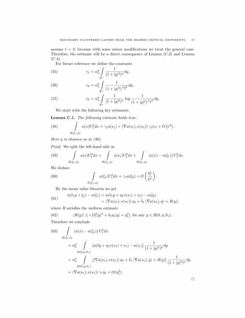
BOUNDARY CLUSTERED LAYERS NEAR THE HIGHER CRITICAL EXPONENTS 17
assume ` = 2, because with some minor modifications we treat the general case.Therefore, the estimate will be a direct consequence of Lemma (C.3) and Lemma(C.4).
For future reference we define the constants
γ1 = αpn
∫Rn
1
(1 + |y|2)ndy,(55)
γ2 = αpn
∫Rn
1
(1 + |y|2)n+22
dy,(56)
γ3 = αpn
∫Rn
1
(1 + |y|2)nlog
1
(1 + |y|2)n−22
dy.(57)
We start with the following key estimates.
Lemma C.1. The following estimate holds true:
(58)
∫B(ξ1,η)
a(x)Up1 dx = γ1a(s1) + 〈∇a(s1), ν(s1)〉 γ1t1ε+O(ε2).
Here η is choosen as in (49).
Proof. We split the left-hand side as∫B(ξ1,η)
a(x)Up1 dx =
∫B(ξ1,η)
a(s1)Up1 dx+
∫B(ξ1,η)
(a(x)− a(ξ1))Up1 dx.(59)
We deduce ∫B(ξ1,η)
a(ξ1)Up1 dx = γ1a(ξ0) +O
(δn1ηn
).(60)
By the mean value theorem we get
(61)a(δ1y + ξ1)− a(ξ1) = a(δ1y + η1ν(s1) + s1)− a(ξ0)
= 〈∇a(s1), ν(s1)〉 η1 + δ1 〈∇a(s1), y〉+R(y),
where R satisfies the uniform estimate
|R(y)| ≤ c(δ21 |y|2 + δ1η1|y|+ η2
1
)for any y ∈ B(0, η/δ1).(62)
Therefore we conclude
(63)
∫B(ξ1,η)
(a(x)− a(ξ1))Up1 dx
= αpn
∫B(0,η/δ1)
[a(δy + η1ν(s1) + s1)− a(s1)]1
(1 + |y|2)ndy
= αpn
∫B(0,η/δ1)
[〈∇a(s1), ν(s1)〉 η1 + δ1 〈∇a(s1), y〉+R(y)]1
(1 + |y|2)ndy
= 〈∇a(s1), ν(s1)〉 γ1η1 +O(η21).

18 NILS ACKERMANN, MONICA CLAPP, AND ANGELA PISTOIA
Lemma C.2. The following estimates hold true:
(64)
∫B(ξ1,η)
a(x)Up−11 (PU1 − U1) dx = −γ2a(s1)ε
(d1
2t1
)n−2
+O(ε1+σ
)and
(65)
∫B(ξ1,η)
a(x)Up−11 PU2dx
=
O(ε1+σ
)ifs1 6= s2,
γ2a(ξ0)ε (d1d2)n−22 ×
×(
1
|t1 − t2|n−2− 1
|t1 + t2|n−2
)+O
(ε1+σ
)if s1 = s2 = ξ0,
for some σ > 0. Here η is choosen as in (49).
Proof. First we prove (64). By Lemma A.1 and Lemma A.2 we get
(66)
∫B(ξ1,η)
a(x)Up−11 (PU1 − U1) dx
=
∫B(ξ1,η)
a(x)Up−11
(−αnδ
n−22
1 H(x, ξ1) +Rδ1,ξ1
)dx
= −αpnδn−21
∫B(0,η/δ1)
a(δ1y + ξ1)H(δ1y + ξ1, ξ1)1
(1 + |y|2)n+22
dy
+O
((δ1η1
)n)= −αpnδn−2
1
∫B(0,η/δ1)
a(δ1y + ξ1)1
|δ1y + ξ1 − ξ1|n−2
1
(1 + |y|2)n+22
dy
+O
((δ1η1
)n−2
η1
)+O
((δ1η1
)n)
= −αpn(δ12η1
)n−2
a(s1)
∫Rn
1
(1 + |y|2)n+22
dy
+O
((δ1η1
)n−1)
+O
((δ1η1
)n−2
η1
),
because
|δ1y + ξ1 − ξ1| = |δ1y + 2η1ν(s1)| ≥ 2η1 − |δ1y| ≥ η1 for any y ∈ B(0, η/δ1).
and by mean value theorem
a(δ1y + ξ1) = a(s1) +O (η1) and1
|δ1y + ξ1 − ξ1|n−2=
1
(2η1)n−2+O
(δ1|y|ηn−1
1
).

BOUNDARY CLUSTERED LAYERS NEAR THE HIGHER CRITICAL EXPONENTS 19
Next, we prove (65). By Lemma A.2
(67)
∫B(ξ1,η)
a(x)Up−11 PU2dx
=
∫B(ξ1,η)
a(x)Up−11
(U2 − αnδ
n−22
2 H(x, ξ2) +Rδ2,ξ2
)dx
= αpn(δ1δ2)n−22
∫B(0,η/δ1)
a(δ1y + ξ1)1
(1 + |y|2)n+22
×
×
(1
(δ22 + |δ1y + ξ1 − ξ2|2)
n−22
dy −H(δ1y + ξ1, ξ2)
)dy
+O
((δ1δ2)
n−22δn+22
2
ηn2
)
= αpn(δ1δ2)n−22
∫B(0,η/δ1)
a(δ1y + ξ1)1
(1 + |y|2)n+22
×
×
(1
(δ22 + |δ1y + ξ1 − ξ2|2)
n−22
− 1
|δ1y + ξ1 − ξ2|n−2
)dy
+O
((δ1δ2)
n−22
ηn−2η2
)+O
((δ1δ2)
n−22δn+22
2
ηn2
)
= αpn(δ1δ2)n−22 a(ξ0)
(1
|η1 − η2|n−2− 1
|η1 + η2|n−2
)∫Rn
1
(1 + |y|2)n+22
dy
+O
((δ1δ2)
n−22
ηn−1
)+O
((δ1δ2)
n−22
ηn−1δ1
)+O
((δ1δ2)
n−22δn+22
2
ηn2
),
because for any y ∈ B(0, η/δ1) we have
|δ1y + ξ1 − ξ2| = |δ1y + (η1 + η2)ν(ξ0)| ≥ η1 + η2 − |δ1y| ≥ η
|δ1y + ξ1 − ξ2| ≥ |ξ1 − ξ2| − |δ1y| ≥ η
and by mean value theorem a(δ1y + ξ1) = a(ξ0) +O (η1) and
1
(δ22 + |δ1y + ξ1 − ξ2|2)
n−22
− 1
|δ1y + ξ1 − ξ2|n−2
=1
|η1 − η2|n−2− 1
|η1 + η2|n−2+O
(δ1|y|+ δ2
2
ηn−1
).

20 NILS ACKERMANN, MONICA CLAPP, AND ANGELA PISTOIA
Lemma C.3. The following estimate holds true:
J0 (Vs,d,t) =2− p
2p[2γ1a(ξ0) + γ1 〈∇a(ξ0), ν(ξ0)〉 ε(t1 + t2)] +
1
2γ2a(ξ0)×
×
[(d1
2t1
)n−2
+
(d2
2t2
)n−2
+ 2 (d1d2)n−22
(1
|t1 − t2|n−2− 1
|t1 + t2|n−2
)]ε
+O(ε1+σ
),
for some σ > 0.
Proof.
J0 (Vs,d,t) =1
2
∫Ω
a(x)|∇Vs,d,t|2dx−1
p
∫Ω
a(x)|Vs,d,t|pdx(68)
We estimate the first term at the R.H.S. of (68). We write
(69)
∫Ω
a(x)|∇Vd,t|2dx
=
∫Ω
a(x)|∇PU1|2dx+
∫Ω
a(x)|∇PU2|2dx− 2
∫Ω
a(x)∇PU1∇PU2dx
Let us estimate the first term in (69). The estimate of the second term is similar.Let us choose η as in (49). We get
(70)
∫Ω
a(x)|∇PU1|2dx = −∫Ω
div (a(x)∇PU1)PU1dx
= −∫Ω
(a(x)∆PU1)PU1dx−∫Ω
〈∇a,∇PU1〉PU1dx
=
∫Ω
a(x)Up−11 PU1dx−
∫Ω
〈∇a,∇PU1〉PU1dx
=
∫B(ξ1,η)
a(x)Up−11 PU1dx+
∫Ω\B(ξ1,η)
a(x)Up−11 PU1dx
−∫Ω
〈∇a,∇PU1〉PU1dx
By (33) we deduce for some β, σ > 0
(71)
∫Ω
〈∇a,∇PU1〉PU1dx ≤ C∫
Ω
|∇PU1|PU1dx = O
(δn−2n−1 +β
1
)= O
(ε1+σ
).
By Lemma A.2 we also deduce
∫Ω\B(ξ1,η)
a(x)Up−11 PU1dx = O
((δ1ε
)n)(72)

BOUNDARY CLUSTERED LAYERS NEAR THE HIGHER CRITICAL EXPONENTS 21
and
∫B(ξ1,η)
a(x)Up−11 PU1dx =
∫B(ξ1,η)
a(x)Up1 dx+
∫B(ξ1,η)
a(x)Up−11 (PU1 − U1) dx.
(73)
The first term is estimated in Lemma C.1 and the second term is estimated in (64)of Lemma C.2.
It remains only to estimate the last term in (69).
(74)
∫Ω
a(x)∇PU1∇PU2dx = −∫Ω
div (a∇PU1)PU2dx
= −∫Ω
(a∆PU1)PU2dx−∫Ω
〈∇a,∇PU1〉PU2dx
=
∫Ω
a(x)Up−11 PU2dx−
∫Ω
〈∇a,∇PU1〉PU2dx.
We have ∫Ω
a(x)Up−11 PU2dx =
∫B(ξ1,η)
· · ·+∫
Ω\B(ξ1,η)
. . .(75)
and
(76)
∫Ω\B(ξ1,η)
a(x)Up−11 PU2dx
= O
δ n+22
1 δn−22
2
∫Ω\B(ξ1,η)
1
|x− ξ1|n+2
1
|x− ξ2|n−2dx
= O
δ n+22
1 δn−22
2
ηn
∫Rn\B(0,1)
1
|y|n+2
1
|y + ξ1−ξ2η |n−2
dy
= O
(δn+22
1 δn−22
2
ηn
)
The first term in (75) is estimated in (65) of Lemma C.2.Finally, as in the proof of (71), from (33) we obtain
(77)
∫Ω
〈∇a,∇PU2〉PU1dx = O(ε1+σ
),
since 0 < C1 ≤ δ2/δ1 ≤ C2 on compact subsets of Λ.

22 NILS ACKERMANN, MONICA CLAPP, AND ANGELA PISTOIA
We estimate the second term at the R.H.S. of (68). We write
(78)
∫Ω
a(x)|Vd,t|pdx =
∫Ω
a(x)|PU1 − PU2|pdx
=
∫Ω
a(x) (|PU1 − PU2|p − |U1|p − |U2|p) dx
+
∫Ω
a(x) (|U1|p + |U2|p) dx.
The last two terms in (78) are estimated in Lemma C.1. Let us choose η as in(49).
We split the first integral as
(79)
∫Ω
a(x) (|PU1 − PU2|p − |U1|p − |U2|p) dx
=
∫B(ξ1,η)
· · ·+∫
B(ξ2,η)
· · ·+∫
Ω\(B(ξ1,η)∪B(ξ2,η))
. . .
From Lemma A.2 we deduce
(80)
∫Ω\(B(ξ1,η)∪B(ξ2,η))
a(x) (|PU1 − PU2|p − |U1|p − |U2|p) dx
= O
∫Ω\(B(ξ1,η)∪B(ξ2,η))
(Up1 + Up2 ) dx
= O
(δn1ηn
+δn2ηn
).
We now estimate the integral over B(ξ1, η).
(81)
∫B(ξ1,η)
a(x) (|PU1 − PU2|p − |U1|p − |U2|p) dx
= p
∫B(ξ1,η)
a(x)Up−11 (PU1 − U1 − PU2) dx
+(p− 1)p
2
∫B(ξ1,η)
a(x)|U1 + θ (PU1 − U1 − PU2) |p−2 (PU1 − U1 − PU2)2dx
−∫
B(ξ1,η)
a(x)|U2|pdx
= p
∫B(ξ1,η)
a(x)Up−11 (PU1 − U1 − PU2) dx+ I,
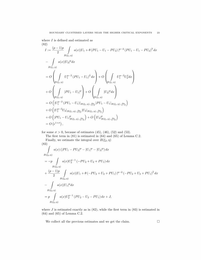
BOUNDARY CLUSTERED LAYERS NEAR THE HIGHER CRITICAL EXPONENTS 23
where I is defined and estimated as(82)
I :=(p− 1)p
2
∫B(ξ1,η)
a(x)|U1 + θ (PU1 − U1 − PU2) |p−2 (PU1 − U1 − PU2)2dx
−∫
B(ξ1,η)
a(x)|U2|pdx
= O
∫B(ξ1,η)
Up−21 (PU1 − U1)
2dx
+O
∫B(ξ1,η)
Up−21 U2
2 dx
+O
∫B(ξ1,η)
|PU1 − U1|p
+O
∫B(ξ1,η)
|U2|pdx
= O
(|Up−2
1 (PU1 − U1)|B(ξ1,η), 2nn+2|PU1 − U1|B(ξ1,η), 2n
n−2
)+O
(|Up−2
1 U2|B(ξ1,η), 2nn+2|U2|B(ξ1,η), 2n
n−2
)+O
(|PU1 − U1|pB(ξ1,η), 2n
n−2
)+O
(|U2|pB(ξ1,η), 2n
n−2
)= O
(ε1+σ
),
for some σ > 0, because of estimates (45), (46), (52) and (53).The first term in (81) is estimated in (64) and (65) of Lemma C.2.Finally, we estimate the integral over B(ξ2, η)
(83)∫B(ξ2,η)
a(x) (|PU1 − PU2|p − |U1|p − |U2|p) dx
= −p∫
B(ξ2,η)
a(x)Up−12 (−PU2 + U2 + PU1) dx
+(p− 1)p
2
∫B(ξ2,η)
a(x)|U1 + θ (−PU2 + U2 + PU1) |p−2 (−PU2 + U2 + PU1)2dx
−∫
B(ξ2,η)
a(x)|U1|pdx
= p
∫B(ξ2,η)
a(x)Up−12 (PU2 − U2 − PU1) dx+ J,
where J is estimated exactly as in (82), while the first term in (83) is estimated in(64) and (65) of Lemma C.2.
We collect all the previous estimates and we get the claim.

24 NILS ACKERMANN, MONICA CLAPP, AND ANGELA PISTOIA
Lemma C.4. The following estimate holds true:
(84)1
p− ε
∫Ω
a(x)|Vs,d,t|p−εdx =1
p
∫Ω
a(x)|Vs,d,t|pdx
+ ε
1
p2
∫Ω
a(x)|Vs,d,t|pdx−1
p
∫Ω
a(x)|Vs,d,t|p−1 log |Vs,d,t|dx
+ o(ε)
= [a(s1) + a(s2)]
(γ1
p2− γ1αn
p− γ3
p
)ε
+n− 2
2pγ1 [a(s1) log δ1 + a(s2) log δ2] ε+ o(ε).
Proof. We argue exactly as in the proof of Lemma 3.2 of [9].
References
[1] A. Bahri and J.M. Coron, On a nonlinear elliptic equation involving the critical Sobolev
exponent: the effect of the topology of the domain, Comm. Pure Appl. Math. 41 (1988),
no. 3, 253–294. MR 89c:35053[2] A. Bahri, Y. Li, and O. Rey, On a variational problem with lack of compactness: the topolog-
ical effect of the critical points at infinity, Calc. Var. Partial Differential Equations 3 (1995),
no. 1, 67–93. MR 1384837 (98c:35049)[3] T. Bartsch, A.M. Micheletti, and A. Pistoia, On the existence and the profile of nodal solu-
tions of elliptic equations involving critical growth, Calc. Var. Partial Differential Equations26 (2006), no. 3, 265–282. MR 2232205 (2007b:35102)
[4] T. Bartsch, A. Pistoia, and T. Weth, N-vortex equilibria for ideal fluids in bounded planar
domains and new nodal solutions of the sinh-Poisson and the Lane-Emden-Fowler equations,Comm. Math. Phys. 297 (2010), no. 3, 653–686. MR 2653899 (2011g:35304)
[5] M. Ben Ayed, K. El Mehdi, O. Rey, and M. Grossi, A nonexistence result of single peaked
solutions to a supercritical nonlinear problem, Commun. Contemp. Math. 5 (2003), no. 2,179–195. MR 1966257 (2004k:35140)
[6] M. Clapp and J. Faya, Multiple solutions to the Bahri-Coron problem in some domains with
nontrivial topology, Proc. Amer. Math. Soc., to appear, 2012.[7] M. Clapp, J. Faya, and A. Pistoia, Nonexistence and multiplicity of solutions to elliptic
problems with supercritical exponents, Calc. Var. Partial Differential Equations, to appear,
2012.[8] M. Clapp and F. Pacella, Multiple solutions to the pure critical exponent problem in domains
with a hole of arbitrary size, Math. Z. 259 (2008), no. 3, 575–589. MR 2395127 (2009f:35076)[9] M. del Pino, P. Felmer, and M. Musso, Multi-bubble solutions for slightly super-critical elliptic
problems in domains with symmetries, Bull. London Math. Soc. 35 (2003), no. 4, 513–521.
MR 1979006 (2004c:35136)[10] M. del Pino, M. Musso, and F. Pacard, Bubbling along boundary geodesics near the second
critical exponent, J. Eur. Math. Soc. (JEMS) 12 (2010), no. 6, 1553–1605. MR 2734352
(2012a:35115)[11] Y. Ge, M. Musso, and A. Pistoia, Sign changing tower of bubbles for an elliptic problem at the
critical exponent in pierced non-symmetric domains, Comm. Partial Differential Equations
35 (2010), no. 8, 1419–1457. MR 2754050 (2011k:35070)[12] D. Gilbarg and N.S. Trudinger, Elliptic partial differential equations of second order, second
ed., Grundlehren der Mathematischen Wissenschaften [Fundamental Principles of Mathemat-
ical Sciences], vol. 224, Springer-Verlag, Berlin, 1983. MR MR737190 (86c:35035)[13] J.L. Kazdan and F.W. Warner, Remarks on some quasilinear elliptic equations, Comm. Pure
Appl. Math. 28 (1975), no. 5, 567–597. MR 0477445 (57 #16972)
[14] E.H. Lieb and M. Loss, Analysis, second ed., Graduate Studies in Mathematics, vol. 14,American Mathematical Society, Providence, RI, 2001. MR 1817225 (2001i:00001)
BOUNDARY CLUSTERED LAYERS NEAR THE HIGHER CRITICAL EXPONENTS 25
[15] M. Musso and A. Pistoia, Multispike solutions for a nonlinear elliptic problem involving the
critical Sobolev exponent, Indiana Univ. Math. J. 51 (2002), no. 3, 541–579. MR 1911045
(2003g:35079)[16] , Sign changing solutions to a nonlinear elliptic problem involving the critical Sobolev
exponent in pierced domains, J. Math. Pures Appl. (9) 86 (2006), no. 6, 510–528. MR 2281450
(2008f:35130)[17] , Tower of bubbles for almost critical problems in general domains, J. Math. Pures
Appl. (9) 93 (2010), no. 1, 1–40. MR 2579374 (2011c:35194)
[18] D. Passaseo, Nonexistence results for elliptic problems with supercritical nonlinearity in non-trivial domains, J. Funct. Anal. 114 (1993), no. 1, 97–105. MR 1220984 (94m:35118)
[19] , New nonexistence results for elliptic equations with supercritical nonlinearity, Dif-
ferential Integral Equations 8 (1995), no. 3, 577–586. MR 1306576 (95j:35086)[20] A. Pistoia and O. Rey, Multiplicity of solutions to the supercritical Bahri-Coron’s problem
in pierced domains, Adv. Differential Equations 11 (2006), no. 6, 647–666. MR 2238023(2007f:35102)
[21] A. Pistoia and T. Weth, Sign changing bubble tower solutions in a slightly subcritical semilin-
ear Dirichlet problem, Ann. Inst. H. Poincare Anal. Non Lineaire 24 (2007), no. 2, 325–340.MR MR2310698 (2008c:35082)
[22] S.I. Pohozaev, On the eigenfunctions of the equation ∆u + λf(u) = 0, Dokl. Akad. Nauk
SSSR 165 (1965), 36–39. MR 0192184 (33 #411)[23] O. Rey, The role of the Green’s function in a nonlinear elliptic equation involving the critical
Sobolev exponent, J. Funct. Anal. 89 (1990), no. 1, 1–52. MR 1040954 (91b:35012)
[24] , Blow-up points of solutions to elliptic equations with limiting nonlinearity, Differ-ential Integral Equations 4 (1991), no. 6, 1155–1167. MR 1133750 (92i:35056)
[25] J. Wei and S. Yan, Infinitely many positive solutions for an elliptic problem with critical orsupercritical growth, J. Math. Pures Appl. (9) 96 (2011), no. 4, 307–333. MR 2832637
Instituto de Matematicas, Universidad Nacional Autonoma de Mexico, Circuito Ex-
terior, C.U., 04510 Mexico D.F., Mexico.
E-mail address: [email protected]
Instituto de Matematicas, Universidad Nacional Autonoma de Mexico, Circuito Ex-terior, C.U., 04510 Mexico D.F., Mexico.
E-mail address: [email protected]
Dipartimento di Metodi e Modelli Matematici, Universita ”La Sapienza” di Roma, viaAntonio Scarpa 16, 00161 Roma, Italia.
E-mail address: [email protected]


