arX

iv:1

603.

0169

4v1

[cs.

IT]

5 M

ar 2

016

1

Intracell Interference Characterization andCluster Inference for D2D Communication

Hafiz Attaul Mustafa1, Muhammad Zeeshan Shakir2, Ali Riza Ekti3,Muhammad Ali Imran1, and Rahim Tafazolli1

1Institute for Communication Systems, University of Surrey, Guildford, UK.{h.mustafa, m.imran, r.tafazolli}@surrey.ac.uk

2Dept. of Systems and Computer Engineering, Carleton University, Ottawa, Canada.muhammad.shakir@sce.carleton.ca

3Dept. of Electrical and Computer Engineering, Gannon University, Erie, PA, U.S.A.alirizaekti@gmail.com

Abstract—The homogeneous poisson point process (PPP) iswidely used to model temporal, spatial or both topologies ofbasestations (BSs) and mobile terminals (MTs). However, negativespatial correlation in BSs, due to strategical deployments, andpositive spatial correlations in MTs, due to homophilic relations,cannot be captured by homogeneous spatial PPP (SPPP). Inthis paper, we assume doubly stochastic poisson process, ageneralization of homogeneous PPP, with intensity measureasanother stochastic process. To this end, we assume PermanentalCox Process (PCP) to capture positive spatial correlation inMTs. We consider product density to derive closed-form ap-proximation (CFA) of spatial summary statistics. We proposeEuler Characteristic (EC) based novel approach to approximateintractable random intensity measure and subsequently derivenearest neighbor distribution function. We further propose thethreshold and spatial extent of excursion set of chi-squarerandomfield as interference control parameters to select different clustersizes for device-to-device (D2D) communication. The spatialextent of clusters is controlled by nearest neighbor distributionfunction which is incorporated into Laplace functional of SPPP toanalyze the effect of D2D interfering clusters on average coverageprobability of cellular user. The CFA and empirical results arein good agreement and its comparison with SPPP clearly showsspatial correlation between D2D nodes.

Index Terms—Intracell interference, D2D communication, Spa-tial correlation, Permanental Cox process, Random field, EulerCharacteristic, Nearest neighbor distribution function.

I. I NTRODUCTION

T HE homogeneous poisson point process (PPP) is char-acterized with remarkable property of complete spatial

randomness. This property is useful when underlying pointsare completely uncorrelated with each other and, subsequently,distributed homogeneously. For example, call arrival in cellularnetworks can precisely be modeled by temporal PPP if weignore traffic inhomogeneity during day and night times.The spatial version of PPP (SPPP) is extensively used tomodel position of base stations (BSs) and mobile terminals(MTs) [1–3]. However, neither BSs/MTs are uncorrelated nordistributed homogeneously. Moreover, due to spatial variationsin traffic, the intensity measure of the point process cannotbeconsidered constant. The inhomogeneity and spatial correla-

tion is usually governed by several dominant factors such asstrategical deployments of BSs, homophilic relations betweenMTs, emergence of mobile social networks, and existence ofhot-spots. As a result, homogeneous PPP is too conservativeto model temporal/spatial topologies of network entities.Suchpoint process cannot precisely model cellular networks sinceit cannot capture negative correlation, in case of BSs, and pos-itive correlation, in case of MTs. The relevant processes thatcapture negative and positive spatial correlations are fermionand boson [4]. These processes can, respectively, be modeledby Determinantal Point Process (DPP) and Permanental CoxProcess (PCP) [5]. The PCP is a doubly stochastic Poissonprocess with intensity measure governed by chi-square randomfield (χ2

k-RF) with k degrees of freedom (df).

A. Related Work

The negative correlation between BSs are modeled usingDPP and Ginibre point process [6–8]. However, to the bestknowledge of authors, the spatial modeling of MTs is restrictedto homogeneous SPPP in the literature. This paper is the firstattempt to model inhomogeneous distribution of MTs withspatial correlation that exists due to any homophilic relation.In this paper, we extend our SPPP approach [9, 10] to PCPmodel with random intensity measure and inhomogeneous dis-tribution to characterize interference in underlay D2D network.To validate simulated realizations, we usednth-order productdensity of PCP to derive Ripley’sK and variance stabilizedL functions. These functions are compared with benchmarkSPPP process to see the deviations. The more upper deviationsmean high positive correlation between points of the process.TheK andL functions of various point processes are available[7, 11], however no analytic expressions for PCP exist inthe literature. The random intensity measure of PCP is ap-proximated by topological inference based on expected EulerCharacteristic (EC) [12]. This approximation is used to derivenearest neighbor distribution function which is introduced intoLaplace functional of SPPP to capture interference due to D2Dpairs. We proposeu andr as interference control parametersto analyze and ensure coverage probability of cellular user.

2

B. Contributions

1) Using nth-order product density of PCP, we deriveKandL functions for exponential covariance function.

2) We propose expected EC based novel approach to ap-proximate random intensity measure of PCP which isgoverned byχ2

k-RF with k df.3) Inspired by statistical parameter mapping (SPM) and

random field theory (RFT) approaches towards func-tional analysis of brain imaging [13]1, we adopted RFTapproach to derive closed-form approximation (CFA) forintractable nearest neighbor distribution functionG.

4) We introduceG function into Laplace functional ofSPPP to capture interference and subsequently deriveCFA for average coverage probability of cellular user inD2D underlay network.

5) We proposeu andr as interference control parameters tocharacterize intracell interference and analyze coverageprobability of cellular user in underlay D2D network.

C. Mathematical Preliminaries

1) Permanental Cox Process:We define spatial point pro-cessΦ in terms of nth-order product density (n). The Φis a random subsetX of underlying locally compact topo-logical/parameter spaceS, a subspace of stratified manifoldM ⊂ R

k. The Φ is said to be PCP process ifX is poissonprocess with random intensity measure defined as [14]:

Λ(B)a.s.=

∫

B

λ(s)ds,

=

∫

B

[Y 21 (s) + · · ·+ Y 2

k (s)]ds,

=

∫

B

χ2kds, (1)

where B ⊆ S is a Borel set,λ(s) is random intensityfunction andY(·)(s) are k independent Gaussian RandomFields (GRFs).

2) Random Field (RF):An RF f = f(t) on M can bedefined as a function whose values are random variables (RVs)for any t ∈M [15]. This function is fully characterized by itsfinite-dimensional distributions (fidi) i.e.,

Ft1,...tk(x1, ..., xk) =p(f(t1) ≤ x1, ..., f(tk) ≤ xk

). (2)

In case, (2) is multivariate Gaussian,f is known as GRF.In real world, not all RFs are Gaussian. Non-Gaussian fieldsform very broader class and are not well defined. Here,we will consider RFs of the formg(t) = G(fm(t)) =G(f1(t), ..., fk(t)) as non-Gaussian or Gaussian related RFs.In casef1(t), ..., fk(t) are zero mean and unit variance GRFs,

1In standard functional analysis of brain and neuroimaging,two approachesare followed to identify activation regions against the null hypothesis (e.g.,z-test, χ2-test, t-test, F-test), (i) Bonferroni correction, (ii) Random FieldTheory. The functional analysis of brain comprises large number of voxelsi.e., large number of statistic values. In case, the statistic values are completelyindependent, the former approach is best to identify activation regions.However, in multiple comparison problem, spatial correlation always existand hence later approach provides less conservative analysis and accurateidentification of activation regions.

we can defineχ2k-RF as [16]:

g(t) =k∑

m=1

f2m(t). (3)

The marginal distribution of (3) for eacht ∈M is χ2 with kdegrees of freedom.

3) Excursion Set:The excursion set,Au above levelu ∈ R,of k-dimensional RF onM is given as [17, 18]:

Au(f,M) , [t ∈M : f(t) ≥ u] ≡ f−1([u,+∞)). (4)

The excursion set of a real-valued non-Gaussian RF can bedefined by applying function compositiong = (G ◦ f) onM . This set is equivalent to the excursion set of vector-valued Gaussianf in G−1[u,+∞), which, under appropriateassumptions onG, is a manifold with piece-wise smoothboundary given by [12]:

Au(g,M

)=Au

((G ◦ f),M

),

={t ∈M : (G ◦ f)(t) ≥ u},={t ∈M : f(t) ∈ G−1[u,+∞)},=M ∩ f−1(G−1[u,+∞)). (5)

Since,G−1[u,+∞) is a specific stratified manifold inRk, wecan generalize it toD ⊂ R

k in (5)

Au(g,M) =M ∩ f−1(D). (6)

4) Lipschitz-Killing Curvature Measures:The Euler Char-acteristicX is a fundamental additive functional that countstopological components ofM . In order to consider boundaries,curvatures, surface area, and volume ofM , the position androtation-invariant generalized functionals are considered whichare known as Lipschitz-killing curvature measures. They arealso known as geometric identifiers that capture intrinsicvolume ofM . For example, in case ofM ⊂ R

2, L0 ≡ X ,L1, L2 gives EC, boundary length, and area of manifoldM . The Lipschitz-killing curvature measuresLj , onBNR , N -dimensional ball of radiusR, is given as [12, Section 6.3]:

Lj(BNR ) =

(Nj

)

RjwNwN−j

, (7)

wherej has dimensionM (i.e.,j = |M |) andωn is the volumeof the unit ball inRn.

D. Organization

The rest of the paper is organized as follows: In Section II,we present system model of cellular network with underlayD2D communication. This is followed by PCP model, forspatial distribution of potential D2D nodes, and details togenerate such a process. To validate the simulated realizationsof PCP, we also derive CFA ofK and L functions inthis section. In Section III, we present the main result ofapproximatingG function of PCP. The CFA ofG function isderived based on expected EC of excursion set ofχ2

k-RF. TheCFA and empiricalG function are compared with SPPP. InSection IV, we introduceG function into Laplace functionalof SPPP to derive CFA for average coverage probability ofcellular user. Conclusion is drawn in Section V.

3

II. SYSTEM MODEL

In this section, we present cellular network model, PCPmodel, process generation, and validation usingK and Lfunctions.

A. Cellular Network Model

The cellular network comprises small cell BS (SBS) andMTs as shown in Fig. 1. We consider orthogonal frequencydivision multiple access (OFDMA) based cellular network. Inthis network, we want to analyze maximum frequency reuseand the effect of interference due to D2D communication. Inorder to avoid coverage holes, SBS should provide homoge-neous coverage for the cellular user. For the homogeneouscoverage at each position in the coverage area, we considerone MT as cellular user which is distributed uniformly. Allother MTs are potential D2D users distributed according toPCP process.

The uplink resources of cellular user are shared by potentialD2D users. The time division duplex (TDD) mode is assumedbetween D2D nodes to capture the effect of interference byboth nodes. In case of frequency division duplex (FDD) mode,the interference at any time instant will simply be half thatofTDD mode. The data and signaling is provided by the servingSBS to the cellular user whereas only signaling is assumedfor potential D2D nodes. For average coverage probability ofcellular user, interference is generated by all successfulD2Dpairs. We consider negligible interference at serving SBS fromsuccessful D2D nodes in neighboring SBSs due to negligiblysmall transmit power.

The cellular and potential D2D users are distributed inthe coverage area bounded between SBS radiusR and theprotection regionR0. The distance between SBS and cellularuser isrc which is used to calculate path-loss at SBS. Everysuccessful D2D pair has a distance ofr between nodes.The channel model assumes distance dependent path-lossand Rayleigh fading. The simple singular path-loss model(rc

−α) is assumed where the protection regionR0 ensuresthe convergence of the model by avoiding nodes to lie atthe origin. The received power at SBS follows exponentialdistribution. The distancerc follows uniform distribution [9]:

f(rc) =2rcR2

, f(θ) =1

2π, (8)

whereR0 ≤ rc ≤ R and0 ≤ θ ≤ 2π.

B. PCP Model

Thenth-order product density(n) of a Cox process is [19]:

(n)(s1, ..., sn) = En∏

i=1

Λ(si), (9)

whereΛ(·) is a random intensity measure. In order to modelspatially correlated process for potential D2D nodes, weconsider PCP with the following intensity measure:

Λ(si) = Y 21 (si) + · · ·+ Y 2

k (si), (10)

whereY(·)(·) are zero mean unit variancek independent real-valued stationary GRFs andY 2

(·)(·) ∼ χ2(·) with unit df.

SBS

Cluster 1

r

D2D Interferer

r

Data Service

Signaling

D2D LinkInterference

Cellular User

R

Ro

rc

Cluster n

Fig. 1: System model for PCP deployed MTs.

The sum of independent chi-square distributions has remark-able property given by the following theorem [20]:

Theorem 1. The sum ofk independent chi-square distribu-tions withvi df follows a chi-square distribution with

∑ki=1 vi

df i.e.,

Z =χ2v1(si) + ...+ χ2

vk(si),

∼ χ2v1+...+vk

(si). (11)

Each squared GRF in (10) has unit df (vi = 1); this resultsin Y 2

(·)(si) ∼ χ2k(si). Therefore, the intensity measure of PCP

is governed byχ2k-RF with k df as:

Λ(si) =χ2k(si). (12)

Since the distribution of potential D2D nodes is translation andmotion invariant, we can assume stationary PCP and henceborrow the definition from [14]:

Definition 1. A Permanental Cox Process is stationary if andonly if the underlying GRF is stationary.

The stationarity of GRF is ensured by underlying covariancefunction. In order to generate smooth GRFs, we considersquared exponential covariance function [21]

C(s1, s2) = e−||s||2

2l2 , (13)

where ||s|| = ||s1 − s2|| =√(s1x − s2x)

2 + (s1y − s2y )2

is the Euclidean distance betweens1 and s2, and l is thecharacteristic length-scale. The resulting covariance matrix ofPCP is represented by[C](s1, ..., sn).

The fact that PCP is a type of Permanental point process isdue to the following theorem [19]:

Theorem 2. Thenth-order product density of Cox process isequal to the weighted permanent of the covariance matrix i.e.,

(n)(s1, ..., sn) = perα[C](s1, ..., sn). (14)

Proof: See, [19, Sec. 2.1.1, p. 876, Theorem 1].

The boson (or photon) process corresponds toα = 1 [22]resulting ink = 2α df for underlying GRFs of PCP.

4

(a) Intensity function of PCP resembles bell-like blobs of GRF. (b) Sampled realization of PCP shows high and low intensity regions.

Fig. 2: Random intensity function of PCP process and sampledhistogram.

C. Process Generation

The random intensity measure of PCP is governed byχ2k-

RF which is non-Gaussian or Gaussian related RF. This fieldis generated by squaring the component field which is GRF(as discussed in Section II-B). The GRF is a collection ofRVs with fidi as multivariate Gaussian. Therefore, it can begenerated by drawing real valued multivariate normal randomvectors and mapping it to the underlying grid. It can also begenerated via circulant embedding method [23]. We followedthe former approach to generate RFs and subsequently PCPprocess. Theχ2

k-RF of PCP comprises large number ofχ2 RVswhich are mapped to each grid points ∈ S. Due to smoothunderlying covariance structure, each RV results into smoothsample path. The blobs and holes show spatial covariancebetweenχ2 RVs. The overall shape of intensity measure ofPCP is similar to symmetric bell-like blobs of GRF, however,the loss of symmetry in this case is due to low df ofχ2

k-RF. Forlarge df, due to central limit theorem, the intensity measure ofPCP resembles symmetric bell-like blobs of GRF.

The lattice representation ofχ2k-RF with 2 df is shown in

Fig. 2(a). In this figure, we can see number of blobs and holeswhich, respectively, show high and low intensity areas. Thehigh intensity areas (7→ 10 on colorbar) capture strong spatialcorrelation between points and results in group clusteringwhereas low intensity areas (1→ 3 on colorbar) form holesdue to nonexistence of any homophilic relation. The Markovchain Monte Carlo based Metropolis-Hasting (MH) sampler2

is used to sample PCP points underχ2k-RF as shown in Fig.

2(b) which shows inhomogeneous and clustered distributionof points.

2The MH sampler is used to sample RVs from multidimensional spaces.The states of the underlying Markov chain can be updated in two differentways, (i) Block-wise, (ii) Component-wise. The first approach updates allstate variables simultaneously whereas the second approach iterates withcomponent-wise update. In both the cases, the acceptance probability is

α = min

(

1,p(θθθ∗)

p(θθθ(t−1))

q(θθθ(t−1)|θθθ∗)

q(θθθ∗|θθθ(t−1))

)

, where p(θθθ) and q(θθθ) stand for

proposal and target distributions, respectively [24].

D. Summary Statistics:K andL Functions

The Ripley’sK function and variance stabilizedL functionsare, respectively, given as [25]:

K(r) =

∫ r

0

g(s)2πsds, (15)

L(r) =

√

K(r)

π, (16)

wherer is the distance andg(s) is the pair correlation function.

Using (14), the first and second order product densities canbe derived as [26]:

= αC(0), (2)(s) = α[1 + C2(s)

]. (17)

Sinceg(s) = (2)(s)/2, the pair correlation function of PCPfor α = 1 is given by:

g(s) =1 + C2(s). (18)

The correspondingK andL functions can be derived as:

K(r) =πr2 + πl2(1− e−( rl)2),

L(r) =

√

r2 + l2(1 − e−( rl)2).

The SPPP is a special case of PCP withg(s) = 1,K(r) = πr2, andL(r) = r. If we assume complete spatialindependence, the covariance betweens1 ands2 vanishes andproduct densities from (17) reduces to:

= α, (2)(s) = α[1 + 0

].

The corresponding pair correlation function (fork = 2 i.e.,α = 1) is 1. TheK andL functions for SPPP can be validatedasK(r) = πr2 andL(r) = r, respectively.

The estimatedK function for SPPP and PCP is, respec-tively, given as [27]:

KSPPP (r) =1

λn

n∑

i=1

n∑

j=1,i6=j

I(si, sj , r),

5

0 5 10 15 200

500

1000

1500

2000

2500

r

K(r)

SPPP: πr2

SPPP: Empirical

PCP: πr2 + πl2(1 − e−( rl)2 )

PCP: Empirical

Fig. 3: CFA and empirical approximations forK function of SPPP and PCP.

KPCP (r) =1

n

n∑

i=1

n∑

j=1,i6=j

I(si, sj, r)

λ(si)λ(sj),

whereλ is the constant intensity function of SPPP,λ(·) is therandom intensity function of PCP andI(·) is the indicatorfunction for the distancer between pointssi and sj . Theanalytic expression ofK and L functions and empiricalestimates are shown in Fig. 3 and Fig. 4, respectively. Asan illustration, the plot is shown for the value ofl = 50. Thisparameter captures the length-scale of the underlying samplepath. In modeling problem, it can be used to incorporate thelevel of covariance in points of the process. We can see thatthe estimates ofK andL functions matches CFA. In thesefigures, SPPP serves as a benchmark with zero correlationbetween points. The positive spatial correlation of PCP canbe verified by upper drift ofK andL functions. In case ofnegative spatial correlation, theK andL functions shall liebelow SPPP curves as can be seen in [6–8].

III. N EAREST NEIGHBOR DISTRIBUTION FUNCTION

In this section, we approximateG function using topolog-ical inference based on expected EC and Poisson clumpingheuristic [28].

A. Nearest Neighbor Distribution Function

The nearest neighbor distribution function of a point processis given as:

G(r) =1− E[e−Λ(BNr )

],

=1− E

[

e−

∫

BNrλ(s)ds

]

, (19)

whereΛ andλ are, respectively, intensity measure and func-tion of point process over closed ball of radiusr at arbitraryposition.

In case of SPPP,λ is constant and hence (19) can besimplified as:

G(r) =1− e−λπr2

. (20)

0 2 4 6 8 10 12 14 16 18 200

5

10

15

20

25

30

r

L(r)

SPPP: rSPPP: Empirical

PCP:√

r2 + l2(1 − e−( rl)2)

PCP: Empirical

Fig. 4: CFA and empirical approximations forL function of SPPP and PCP.

ConsideringΛ from (12), the nearest neighbor distributionfunction of PCP is given as:

G(r) =1− E

[

e−

∫

BNrχ2k ds

]

,

=1− E

[

e−

∫

BNr

∫

v1···

∫

vnχ2dv1···dvn ds

]

. (21)

Since χ2k-RF is a collection of large number of RVs, this

results in evaluation of nested integrals overBNr whichis mathematically intractable. In this case, we approximateintensity measureΛ using expected EC of excursion set ofχ2k-RF [12].

1) Approximation of Intensity Measure:The expected in-tensity measure in (21) can be estimated by making topologicalinference of average number of upcrossings ofχ2

k-RF abovelevel u of excursion set. This approach is based on GaussianKinematic Formulae (GKF) given as [12, Theorem 15.9.4]:

Theorem 3. Let M be anN -dimensional, regular stratifiedmanifold, D a regular stratified subset ofRk. Let f =(f1, ..., fk) :M → R

k be a vector-valued Gaussian field, withindependent, identically distributed components andf beingMorse function3 overM with probability one. Then

E[Li(M ∩ f−1(D))

]=

N−i∑

j=0

[i+ jj

] Li+j(M)Mj(D)

(2π)j2

,

(22)

whereLi+j for i = 0, ..., N, j = 0, ..., N − i, are Lipschitz-Killing curvature measures onM with respect to the metric in-duced byf andMj are the generalized (Gaussian) Minkowskifunctionals onRk.

For notational convenience, we assume the combinatorial

3For the definition of Morse function and Morse’s Theorem, refer [29,Theorem 4.4.1, pp. 87] and [24, Section 9.3, Definition 9.3.1, pp. 206].

6

0 5 10 15 20 25 300

0.1

0.2

0.3

0.4

0.5

0.6

0.7

0.8

u

EC

Den

sity

ρ0(u)

ρ1(u)

ρ2(u)

Fig. 5: EC density representing density of unit component ofχ2k

-RF thatsurvives thresholdu.

flag coefficients

[i+ jj

]

=

[ab

]

given as:

[ab

]

=[a]!

[b]![a− b]!, [a]! = a!ωa, ωa =

πa2

Γ(a2 + 1).

Using Theorem 3 and puttingM ∩ f−1(D) from (6), theexpected intensity measure can be approximated as follows:

ψ0 ≈E[χ2k(B

Nr )

],

=E[L0

(Au(χ

2k, B

Nr )

)],

=

N∑

j=0

Lj(BNr )Mj(D)

(2π)j2

. (23)

The Minkowski functionalsMj(D) can be transformed intoEC density forχ2

k-RF as [12]:

ψ0 =

N∑

j=0

ρj(u)Lj(BNr ), (24)

where

ρj(u) =uk−j2 e−

u2

(2π)j2Γ(k2 )2

k−22

⌊ j−12 ⌋

∑

l=0

j−1−2l∑

m=0

× 1{k≥j−m−2l}

(k − 1

j − 1−m− 2l

)

× (−1)j−1+m+l(j − 1)!

m!l!2lum+l.

The EC density overR2 and average upcrossings ofχ2k-

RF are shown in Fig. 5 and Fig. 6, respectively. In Fig. 5,a very interesting fact can be observed forρ0. The value ofj = 0 transformsN dimensional ManifoldM to a single pointwhere spatial correlation does not make sense. In this case,ECdensity reduces toχ2 distribution with k df conforming thefact that marginal distribution ofχ2

k-RF isχ2 distributed [16].In Fig. 6, the behavior ofχ2

k-RF for differentu is plotted withrespect to differentLi measures. In this paper, we considerL0

(i.e., EC) to approximate intensity measure of PCP process.

0 5 10 15 20 25 300

0.5

1

1.5

2

2.5

3x 10

4

AverageUpcrossings

u

E{L0(Au(χ2k, S))}

E{L1(Au(χ2k, S))}

E{L2(Au(χ2k, S))}

Fig. 6: Average number of components ofχ2k

-RF for different Lipschitz-killing curvature measures over 200× 200 square grid.

2) Poisson Clumping Heuristic4: To approximate nearestneighbor distribution function, we consider probability ofgetting one, or more, clusters (D2D pairs) with spatial extentr, or more, above thresholdu. The general expression for thiscluster level inference is given as [13, 31]:

G(r) ≃ 1− e−ψ0 p(v≥r). (25)

The volumev of clusters (D2D pairs) over spatial extentr isdistributed according to [32]:

p(v ≥ r) ≈ e

(−βr

2N

)

, (26)

where

β =

(Γ(N2 + 1)

η

) 2N

,

andη = ρ0vLN/ψ0 is the expected volume of each cluster.

The plots ofη andp(v ≥ r) are shown in Fig. 7 and Fig.8, respectively. In these figures, we can see that the maximumexpected volume and the probability to have nodes with spatialextent (≥)r occurs forv = 1. In deriving CFA ofG function,we, considerη for v = 1.

Using (7), the Lipschitz-Killing curvature measuresLj overball of spatial extentr can be derived as:

L0 = 1, (27a)

L1 = 2√πr

Γ(12 + 1)

Γ(2), (27b)

L2 = πr2Γ(1)

Γ(2). (27c)

Considering (27), (24), and (26) in (25) for, at most, distancer, theG function can be approximated. The plot ofG functioncan be seen in Fig. 9 where PCP points, due to positivespatial correlation, have higher probability of D2D pairs as

4At high thresholds, the clusters in the excursion set can be regarded asmultidimensional point process with no memory and hence they behave aspoisson clumps [30].

7

0 5 10 15 20 250

1

2

3

4

5

6

7

Cluster Number (v)

Expectedvolumeofea

chcluster

Fig. 7: Expected volume of each cluster depends on EC density, volume ofunderlying space, and expected EC. The plot is drawn foru = 31.

compared to SPPP points. For example, at a distance of 2.5 m,the probability of two spatially correlated potential candidatesfor D2D communication is 0.8 as compared to 0.42 in SPPPpoints which occur so close by chance (i.e., not due to spatialcorrelation under some homophilic relation). This is becauseSPPP cannot model spatial correlation between points and ischaracterized by complete spatial randomness.

IV. AVERAGE COVERAGE PROBABILITY

In this section, we introduceG function as retention prob-ability of D2D nodes at spatial extentr to analyze theinterference and resulting average coverage probability ofcellular user. We assume interference-limited environment dueto large number of potential D2D pairs. Hence, the signal-to-interference ratio (SIR) is given as:

SIRSBS =pcfcr

−αc

∑

i∈Φ pifir−αi

, (28)

wherepc andpi are transmit powers of cellular user and D2Dinterferers, respectively;fc, andfi are respective small-scalefading. The corresponding distance dependent path-loss arer−αc andr−αi . Assuming exponential distribution with mean1 for power received by SBS, the average coverage probabilityof uplink cellular user is given by the following theorem.

Theorem 4. The average coverage probability of a cellularuser with underlay D2D communication is

pccov =

∫ R

R0

e−

2π2ψ0p(r) r2c

α sin( 2πα

)

(γpc

) 2αE[p

2αi ] 2rc

R2drc. (29)

Proof: See Appendix A.For same transmit power of all D2D interferers, the average

coverage probability of cellular user for path-loss exponentα = 4 andR0 ∼ 0 reduces to:

pccov =e−π2R2ψ0p(r)

2

√

γpipc − 1

−π2R2ψ0p(r)2

√γpipc

. (30)

0 5 10 15 20 250

0.1

0.2

0.3

0.4

0.5

0.6

0.7

0.8

0.9

1

Cluster Number (v)

p(v

≥r)

r = 1 mr = 2 mr = 4 mr = 8 m

Fig. 8: The probability of clusterv with different spatial extentsr isexponentially distributed with meanβ

(

see Eq. (26))

.

V. NUMERICAL RESULTSAND DISCUSSION

In this section, we numerically evaluate the analytic expres-sions of Sec. IV by varying the number of different parameters.The average coverage probability of cellular user in (30)depends onR, ψ0 (and an important implicit parameteru),spatial extentr, D2D transmit powerpi, transmit power ofcellular userpc, and target thresholdγ. The first and foremoststep is to identify implicit parameteru which is introduced asinterference control parameter for D2D pairing. This parameteris a function of grid size and more specifically SBS radiusR. By finding the feasible range ofu for a given radiusR,we have varied other parameters to analyze average coverageprobability of cellular user. For different spatial extents r, thecumulative interference effect is captured. Since the distancebetween D2D pairs is much smaller as compared to distancebetween D2D pair and SBS, it is reasonable to assume sametransmit power for every D2D pair in the coverage area. To

0 5 10 15 200

0.1

0.2

0.3

0.4

0.5

0.6

0.7

0.8

0.9

1

r

G(r)

SPPP: 1 − e−λπr2

SPPP: Empirical

PCP: CFAPCP: Empirical

Fig. 9: Nearest neighbor distribution function of PCP showshigh probabilityfor lower values ofr as compared to homogeneous SPPP process.

8

(a) Intensity function of PCP on 200×200 grid for thresh-old valuesu = (1, 2, 4, 8).

(b) 10×10 extract of Fig. 10(a) clearly shows survivingand departing blobs at same values ofu.

−5

0

5

10

15

20

0

10

20

30

400

0.2

0.4

0.6

0.8

1

γ(dB)u

pc cov

(c) Coverage probability of cellular user drops for lowvalues ofu i.e., maximum number of possible D2D pairs.

Fig. 10: Interference characterization in terms of intensity measure of PCP at different values ofu (Fig. 10(a), 10(b)) and average coverage probability ofcellular user (Fig. 10(c)) forpi = 0 dBm,pc = 20 dBm, andR = 100 m.

analyze the interference due to D2D clusters, we introducenearest neighbor distribution function into Laplace functionalof SPPP.

In Fig. 10, we show intensity function at different thresholdsand corresponding average coverage probability of cellularuser for grid size 200×200 (SBS of radiusR = 100 m).For clear illustration, the small portion of this grid has beenshown in Fig. 10(b). In this grid, if we setu = 2 (transparentblack plane), all nodes (despite low spatial correlation) will beconsidered to make D2D pairs5 based on the spatial distancer. This results in maximum intracell interference and causesblockage for the cellular user. If we increaseu (red, green,and blue transparent planes), only those potential D2D pairswill survive that lie under high intensity blobs ofχ2

k-RF.In this case, the coverage probability of cellular user canbe ensured while reusing the resources for D2D pairs. Thecoverage probability curves for differentu andγ can be seenin Fig. 10(c). The high threshold, for example,u = 35 inthis figure shows no D2D pair and ensure the unit coverageprobability of cellular user.

The interference control parameteru for different grid sizeshas been plotted in Fig. 11. In this figure, it can be seenthat the interference, due to D2D communication on coverage

5The maximum number of upcrossings ofχ2k

-RF occurs at aroundu = kas can be verified in Euler density (Fig. 5) and expected EC (Fig. 6) plots.

probability of cellular user, is captured byu. As an example,for 10×10 grid size (SBS of radiusR = 5 m), thepccov risesfrom 2% to 98% foru = 5 to 16 as compared to 1000×1000grid size (R = 500 m) where the blockage extends on the floorupto the value ofu = 37 and shows 98% rise inpccov at u =45.

5 10 15 20 25 30 35 40 450

0.1

0.2

0.3

0.4

0.5

0.6

0.7

0.8

0.9

1

Interference threshold (u)

Coverageprob.ofcellularuser

10× 10200× 200500× 5001000× 1000

(27, 0.02) (35, 0.98)

Fig. 11: Interference control parameteru for different grid sizes (SBS radiusR) for pi = 0 dBm,pc = 20 dBm.

9

−5 0 5 10 15 200

0.1

0.2

0.3

0.4

0.5

0.6

0.7

0.8

0.9

1

Target SIR (γ(dB))

Coverageprob.ofcellularuser

C1 <= 16 mC2 <= 8 mC3 <= 4 mC4 <= 2 m

Fig. 12: Clusters of D2D nodes and coverage probability of cellular user foru = 31, pi = 0 dBm,pc = 20 dBm andR = 100 m.

In Fig. 12, we have shown the effect of interference dueto different cluster sizes on coverage probability of cellularuser. The cluster sizes show different number of D2D nodesthat survive the thresholdu. For example, atu = 31 (pccov =0.62 from Fig. 11), four cluster sizes ofr = (16, 8, 4, 2)mare shown that consider D2D communication by reusingthe frequency of cellular user. The maximum cluster sizeconsiders all nodes which are less than or equal to 16 m forD2D communication and hence causes maximum interference.Contrary to this, the minimum cluster size considers nodeswith 2m or less distance for D2D communication and henceresults in less interference.

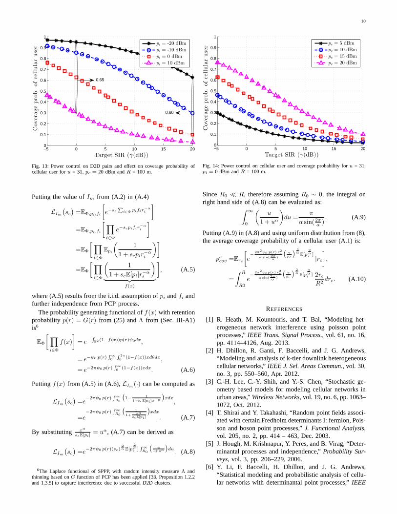
The effect of power control on D2D pairs can be seen in Fig.13. In this figure, we can see that the coverage probability ofcellular user can be ensured by controlling the transmit powerof successful D2D pairs. The coverage drop at two values ofγ (0 and 20 dB) is approximately equal, however, two curveswith smallerpi ([-20 -10] dBm) converges rapidly at lowervalues ofγ as compared to curves with highpi ([0 10] dBm).This trend is reversed at high values ofγ.

The effect of power control on cellular user and coverageprobability curves are shown in Fig. 14. It can be seen that thecurves for differentpc converge to low coverage probabilityfor highγ. The coverage probability can be increased by eitherreducing transmit power of D2D pairs or reducing the numberof D2D pairs by increasing thresholdu. The thresholdu andspatial extentr (small r requires lowerpi) are key controlparameters to ensure the extent of frequency reuse (D2D pairs)while ensuring coverage probability of cellular user.

VI. CONCLUSION

In this paper, we proposed PCP process to model inho-mogeneous and spatially correlated distribution of MTs. Weconsidered this process to characterize intracell interference inD2D underlay network. We further approximated intractablenearest neighbor distribution function by adopting expectedEuler Characteristic and Poisson clumping heuristic. The keyfindings of this research are enumerated as:

1) Simple SPPP process with constant intensity measurecannot capture prevailing inhomogeneity and spatialcorrelation in dense cellular networks. Therefore, pointprocesses with attraction/repulsion property (e.g., Coxprocess/DPP) are potential candidates for precise spatialmodeling of MTs/BSs.

2) Euler Characteristic and RFT framework can be usedto analyze and identify high intensity areas/hotspots forD2D communication.

3) Provided SPMs of coverage area are available, statisticalinference can be performed to identify clusters of MTswith high spatial correlation (potential areas for D2Dcommunication).

4) The intensity measure of PCP is governed byχ2k-RF.

In this case the thresholdu of the excursion set playsa key role to control cluster size, for D2D communica-tion, level of interference, due to frequency reuse, andcoverage probability of cellular user.

APPENDIX A - PROOF OFTHEOREM 4

The average coverage probability of uplink cellular userdistributed uniformly over plane betweenR and R0 at adistancerc from the serving SBS is given as follows:

pccov =Erc

[p(SIRSBS ≥ γ

)| rc

],

=Erc

[

p(fc ≥

γIm

pcr−αc

)| rc

]

, (A.1)

where

Im =∑

i∈Φ

pifir−αi , (A.2)

is the cumulative interference due to D2D clusters in thecoverage area andE(·) is expectation with respect to (·).

In (A.1), the coverage probability depends on number ofRVs e.g.,pc, fc, r−αc , pi, fi, r

−αi . The power transmitted by

the cellular userpc is assumed to be independent of theinterferers. The serving SBS uses uplink power control toensure quality of service of the cellular user based on distancedependent path-loss. The fadingfc and fi follows Rayleighdistribution with pc and pi as exponentially distributed. Thecellular user is uniformly distributed in the coverage areawhereas all potential D2D nodes are distributed accordingto PCP process. Conditioning ong = {pi, fi}, the coverageprobability of cellular user for a given transmit powerpc is:

p(SIRSBS ≥ γ

)| rc, g =

∫ ∞

x= γIm

pcr−αc

e−xdx,

=e−γp−1c rαc Im . (A.3)

De-conditioning byg, (A.3) results in

p(SIRSBS ≥ γ

)| rc =Eg

[e−γp

−1c rαc Im

],

=Eg

[e−scIm

],

=LIm(sc), (A.4)

wheresc = γp−1c rαc .

10

−5 0 5 10 15 200

0.1

0.2

0.3

0.4

0.5

0.6

0.7

0.8

0.9

1

Target SIR (γ(dB))

Coverageprob.ofcellularuser

pi = -20 dBm

pi = -10 dBm

pi = 0 dBm

pi = 10 dBm

0.60

0.65

Fig. 13: Power control on D2D pairs and effect on coverage probability ofcellular user foru = 31, pc = 20 dBm andR = 100 m.

Putting the value ofIm from (A.2) in (A.4)

LIm(sc)=EΦ,pi,fi

[

e−sc∑

i∈Φ pifir−αi

]

=EΦ,pi,fi

[∏

i∈Φ

e−scpifir−αi

]

=EΦ

[∏

i∈Φ

Epi

(1

1 + scpir−αi

)]

=EΦ

[∏

i∈Φ

(1

1 + scE[pi]r−αi

)

︸ ︷︷ ︸

f(x)

]

, (A.5)

where (A.5) results from the i.i.d. assumption ofpi andfi andfurther independence from PCP process.

The probability generating functional off(x) with retentionprobability p(r) = G(r) from (25) andΛ from (Sec. III-A1)is6

EΦ

[∏

i∈Φ

f(x)

]

= e−∫

R2(1−f(x))p(r)ψ0dx,

= e−ψ0 p(r)∫ ∞0

∫ 2π0

(1−f(x))xdθdx,

= e−2πψ0 p(r)∫ ∞0

(1−f(x))xdx. (A.6)

Puttingf(x) from (A.5) in (A.6),LIm(·) can be computed as

LIm(sc)=e

−2πψ0 p(r)∫∞R0

(1− 1

1+scE[pi]x−α

)xdx

,

=e−2πψ0 p(r)

∫

∞R0

(1

1+ xα

scE[pi]

)xdx

. (A.7)

By substituting xα

scE[pi]= uα, (A.7) can be derived as

LIm(sc)=e

−2πψ0 p(r)(sc)2α E[p

2αi

]∫ ∞R0

(u

1+uα

)du. (A.8)

6The Laplace functional of SPPP, with random intensity measure Λ andthinning based onG function of PCP has been applied [33, Proposition 1.2.2and 1.3.5] to capture interference due to successful D2D clusters.

−5 0 5 10 15 200

0.1

0.2

0.3

0.4

0.5

0.6

0.7

0.8

0.9

1

Target SIR (γ(dB))

Coverageprob.ofcellularuser

pc = 5 dBm

pc = 10 dBm

pc = 15 dBm

pc = 20 dBm

Fig. 14: Power control on cellular user and coverage probability for u = 31,pi = 0 dBm andR = 100 m.

SinceR0 ≪ R, therefore assumingR0 ∼ 0, the integral onright hand side of (A.8) can be evaluated as:

∫ ∞

0

(u

1 + uα

)

du =π

α sin(2πα). (A.9)

Putting (A.9) in (A.8) and using uniform distribution from (8),the average coverage probability of a cellular user (A.1) is:

pccov =Erc

[

e−

2π2ψ0 p(r) r2c

α sin( 2πα

)

(γpc

) 2αE[p

2αi

]|rc

]

,

=

∫ R

R0

e−

2π2ψ0p(r) r2c

α sin( 2πα

)

(γpc

) 2αE[p

2αi

] 2rcR2

drc. (A.10)

REFERENCES

[1] R. Heath, M. Kountouris, and T. Bai, “Modeling het-erogeneous network interference using poisson pointprocesses,”IEEE Trans. Signal Process., vol. 61, no. 16,pp. 4114–4126, Aug. 2013.

[2] H. Dhillon, R. Ganti, F. Baccelli, and J. G. Andrews,“Modeling and analysis of k-tier downlink heterogeneouscellular networks,”IEEE J. Sel. Areas Commun., vol. 30,no. 3, pp. 550–560, Apr. 2012.

[3] C.-H. Lee, C.-Y. Shih, and Y.-S. Chen, “Stochastic ge-ometry based models for modeling cellular networks inurban areas,”Wireless Networks, vol. 19, no. 6, pp. 1063–1072, Oct. 2012.

[4] T. Shirai and Y. Takahashi, “Random point fields associ-ated with certain Fredholm determinants I: fermion, Pois-son and boson point processes,”J. Functional Analysis,vol. 205, no. 2, pp. 414 – 463, Dec. 2003.

[5] J. Hough, M. Krishnapur, Y. Peres, and B. Virag, “Deter-minantal processes and independence,”Probability Sur-veys, vol. 3, pp. 206–229, 2006.

[6] Y. Li, F. Baccelli, H. Dhillon, and J. G. Andrews,“Statistical modeling and probabilistic analysis of cellu-lar networks with determinantal point processes,”IEEE

11

Trans. Commun., vol. 63, no. 9, pp. 3405–3422, Sep.2015.

[7] N. Deng, W. Zhou, and M. Haenggi, “The ginibre pointprocess as a model for wireless networks with repulsion,”IEEE Trans. Wireless Commun., vol. 14, no. 1, pp. 107–121, Jan. 2015.

[8] Y. Li, F. Baccelli, H. S. Dhillon, and J. G. Andrews,“Fitting determinantal point processes to macro base sta-tion deployments,”in Proc. Intl. Conf. Global Communs.,GLOBECOM’2014, Austin, TX, USA, Dec. 2014.

[9] H. Mustafa, M. Shakir, M. Imran, A. Imran, and R. Tafa-zolli, “Coverage gain and device-to-device user density:Stochastic geometry modeling and analysis,”IEEE Com-mun. Lett., vol. 19, no. 10, pp. 1742–1745, Oct. 2015.

[10] H. Mustafa, M. Shakir, M. Imran, and R. Tafazolli,“Distance based cooperation region for D2D pair,”inProc. Vehicular Technology Conf., VTC’2015, Glasgow,Scotland, May 2015.

[11] F. Lavancier, J. Møller, and E. Rubak, “Determinantalpoint process models and statistical inference,”J. R.Statist. Soc. B, vol. 77, no. 4, pp. 853–877, Sep. 2015.

[12] R. J. Adler and J. E. Taylor,Random Fields and Geom-etry, 1st ed. New York, USA: Springer-Verlag, 2007.

[13] K. Friston,Statistical Parametric Mapping: The Analysisof Functional Brain Images, 1st ed. London, UK:Academic Press, 2007.

[14] J. Møller, A. R. Syversveen, and R. P. Waagepetersen,“Log Gaussian Cox processes,”Scandinavian Journal ofStatistics, vol. 25, no. 3, pp. 451–482, 1998.

[15] P. Abrahamsen and N. regnesentral, “A Review of Gaus-sian Random Fields and Correlation Functions,” NorskRegnesentral, Norwegian Computing Center, Oslo, Nor-way, Tech. Rep. 917, 1997.

[16] K. J. Worsley, “Local maxima and the expected Eulercharacteristic of excursion sets ofχ2, F and t fields,”Advances in Applied Probability, pp. 13–42, 1994.

[17] R. J. Adler and A. M. Hasofer, “Level crossings forrandom fields,”The Annals of Probability, vol. 4, no. 1,pp. 1–12, Feb. 1976.

[18] R. J. Adler, “Excursions above a fixed level by n-dimensional random fields,”J. Applied Probability,vol. 13, no. 2, pp. 276–289, 1976.

[19] P. McCullagh and J. Møller, “The permanental process,”Advances in Applied Probability, vol. 38, no. 4, pp. 873–

888, Dec. 2006.[20] S. M. Ross,Introduction to Probability and Statistics

for Engineers and Scientists, 4th ed. Boston, USA:Academic Press, Mar. 2009.

[21] C. E. Rasmussen and C. K. I. Williams,Gaussian Pro-cesses for Machine Learning. Massachusetts, USA: MITPress, Jan. 2006.

[22] O. Macchi, “The coincidence approach to stochasticpoint processes,”Advances in Applied Probability, vol. 7,no. 1, pp. 83–122, 1975.

[23] E. Spodarev,Stochastic Geometry, Spatial Statistics andRandom Fields: Asymptotic Methods, 1st ed. Heidel-berg, Germany: Springer-Verlag, Feb. 2013.

[24] W. L. Martinez and A. R. Martinez,Computational

Statistics Handbook with Matlab, 2nd ed. Florida, USA:CRC Press, Dec. 2007.

[25] B. D. Ripley, “The second-order analysis of stationarypoint processes,”J. Applied Probability, vol. 13, no. 2,pp. 255–266, Jun. 1976.

[26] J. Møller and P. McCullagh, “The permanent process,”Aalborg University, Department of Mathematical Sci-ences, Aalborg, Denmark, Tech. Rep. R-2005-29, 2005.

[27] E. Marcon and F. Puech, “Generalizing Ripley’s K func-tion to inhomogeneous populations,”preprint, Apr. 2009.

[28] J. Cao, “The size of the connected components of ex-cursion sets ofχ2, t and F fields,”Advances in AppliedProbability, vol. 31, no. 3, pp. 579–595, 1999.

[29] R. J. Adler,The Geometry of Random Fields. Philadel-phia, USA: Society for Industrial and Applied Mathe-matics, Dec. 2009.

[30] D. Aldous, Probability Approximations via the PoissonClumping Heuristic, 1st ed. New York, USA: Springer-Verlag, Mar. 2013.

[31] J. C. Mazziotta, A. W. Toga, and R. S. J. Frackowiak,Brain Mapping: The Disorders. San Diego, USA:Academic Press, May 2000.

[32] K. J. Friston, K. J. Worsley, R. S. J. Frackowiak, J. C.Mazziotta, and A. C. Evans, “Assessing the significanceof focal activations using their spatial extent,”HumanBrain Mapping, vol. 1, no. 3, pp. 210–220, Jan. 1994.

[33] F. Baccelli and B. Błaszczyszyn, “Stochastic geometryand wireless networks: volume I theory,”Foundationsand Trends in Networking, vol. 3, no. 34, pp. 249–449,2008.