Smooth inversion, Plus-Minus, Wavefront layer refraction of 7 shots into 24 receivers :

Fig. 1 : Velocity tomogram obtained with Smooth inversion with default settings and 20 WET iterations.

Layer-based Plus-Minus refractors are plotted in magenta and brown, see Fig. 3 below.

Fig. 2 : WET wavepath coverage plot obtained with tomogram shown in Fig. 1

We recommend shooting at every 3rd receiver, not just every 6th receiver. Import the data into a Rayfract® profile and run our Smooth inversion and Plus-Minus methods, with our free trial :

- create a new profile with File|New Profile…, set File name to JENNY13 and click Save button - unzip jenny13.zip in \RAY32\JENNY13\INPUT directory - specify a Station spacing of 5m in Header|Shot, before importing the data.

- check File|Import Data Settings|Keep same Layout start for consecutive shot files - check File|Import Data Settings|Default layout start is 1.0 - select File|Import Data… and specify Import data type SEG-2 - click upper Select button, navigate into \RAY32\JENNY13\INPUT and select 2001.DAT - set Default spread type to 01: 24 channels - click Open button and Import shots button - leave Layout start at 1 for all shots - specify Shot pos. [station no.] -5.5, 0.5, 6.5, 12.5, 18.5, 24.5, 30.5, click Read for shots 1 to 7 - select File|Update header data|Update First Breaks… - navigate into \RAY32\JENNY13\INPUT directory and select file BREAKS.LST, click Open - select Smooth invert|WET with 1D-gradient initial model… - confirm prompts for 1D starting model, WET tomogram and wavepath coverage (Fig. 1, Fig. 2)

Iteratively vary mapping of traces to refractors in Refractors|Shot breaks, select Depth|Plus-Minus and Velocity|Plus-Minus until Plus-Minus interpretation (Fig. 3) matches Smooth inversion tomogram (Fig. 1). In Depth|Plus-Minus, press ALT+M keyboard shortcut and decrease Base filter width [station nos.] to 5, from default value 10. Hit ENTER key to recompute and redisplay Plus-Minus depth and velocity sections. See our release notes for latest version 3.25 and Grid menu options (Fig. 6) for plotting of refractors on WET tomograms. To redisplay the WET tomogram with Plus-Minus refractors :

- select Depth|Plus-Minus and File|Export header data|Export ASCII Model of depth section... - click Save button to export Plus-Minus refractors and layer velocities to file PLUSMODL.CSV - select Grid|Select ASCII .CSV layer model for refractor plotting... and above PLUSMODL.CSV - check Grid menu options for refractor plotting as shown in Fig. 6 - select Grid|Image and contour velocity and coverage grids… - select tomogram grid file \RAY32\JENNY13\GRADTOMO\VELOIT20.GRD to obtain Fig. 1

Fig. 3 : Layer-based Plus-Minus refraction interpretation, 3 layers. Left : interactively map traces to refractors.

Center : Depth section obtained with Plus-Minus method. Right : Plus-Minus Velocity section.

Fig. 4 : Edit Base map and refractor polyline properties in Surfer’s Object Manager.

Fig. 5 : Trace|Offset gather (left), Trace|Shot gather (center), Refractor|Shot breaks (right). Browse offset gathers with

F7/F8 in Trace|Offset gather, to quality-check for reciprocal traveltime errors. Note asymmetry of first breaks for shot no. 4 (center), relative to shot point (station no. 12.5). This indicates a dipping basement refractor, as indicated in Trace|Offset gather (left) and Refractor|Shot breaks (right).

Quality-check your first break picks for reciprocal traveltime errors in Trace|Offset gather, see Fig. 5. and riveral8 tutorial. Browse common-offset sorted trace gathers with F7/F8 function keys. Edit refractor polyline properties line style, color, width and end styles as in Fig. 4, in Golden Software Surfer’s Object Manager.

Our layer-based Plus-Minus refraction (Fig. 3), Wavefront refraction and CMP Intercept-time refraction methods can use far-offset shots no. 1 and no. 7 positioned at station nos. -5.5 and 30.5. Offset shots no. 1 and no. 7 cannot be used for 2D WET inversion, since there are no receivers near these shot points, at station no. -5.5 and 30.5 . Use overlapping receiver spreads, for our WET inversion to be able to use profile-internal offset shots. Also see our .pdf reference topics Mapping traces to refractors, Time-to-depth conversion and Overlapping receiver spreads.

Fig. 6 : Grid menu options, for Rayfract® version 3.25

Fig. 7 : Refractor|Midpoint breaks, mapping traces to refractors with ALT+M and 1D velocity model

Fig. 8 : left : Refractor|Midpoint breaks, center : Velocity|Wavefront, right : Depth|Wavefront

Fig. 9 : Velocity tomogram obtained with Smooth inversion with default settings and 20 WET iterations.

Layer-based Wavefront method refractors are plotted in magenta and brown. Compare Fig. 8.

To obtain Fig. 9 overlaying Wavefront method refractors on WET tomogram : - select Refractor|Midpoint breaks, press ALT+M. Edit mapping parameters as in Fig. 7 - set Refracted Wave Offset Delta to 5, Weathering to 750 m/s and Refractor 1 to 1550 m/s - hit ENTER key to map traces to refractors. - press ALT+G for Crossover distance processing dialog, edit as in Fig. 10 - leave Basement filter [station nos.] at 10, click Accept button to smooth crossover distance - press CTRL+F1 to zoom dip of CMP curves in Fig. 7 - select Depth|Wavefront, press ALT+M, edit model parameters as in Fig. 11

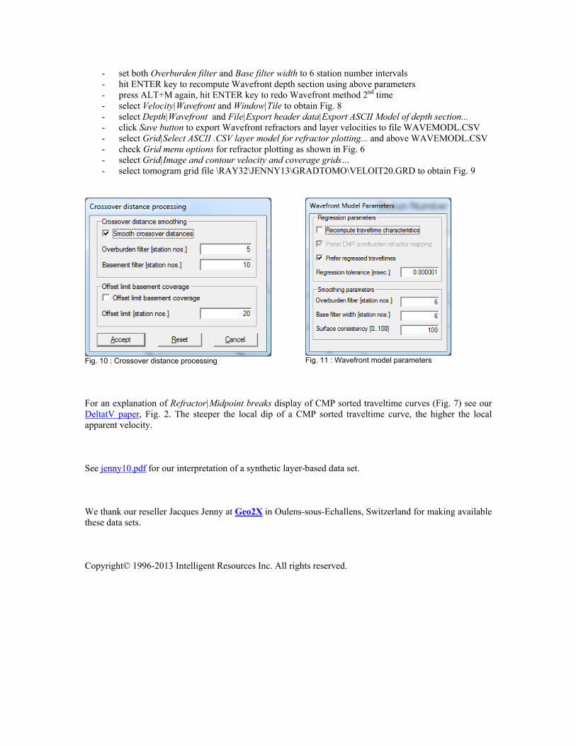
- set both Overburden filter and Base filter width to 6 station number intervals - hit ENTER key to recompute Wavefront depth section using above parameters - press ALT+M again, hit ENTER key to redo Wavefront method 2nd time - select Velocity|Wavefront and Window|Tile to obtain Fig. 8 - select Depth|Wavefront and File|Export header data|Export ASCII Model of depth section... - click Save button to export Wavefront refractors and layer velocities to file WAVEMODL.CSV - select Grid|Select ASCII .CSV layer model for refractor plotting... and above WAVEMODL.CSV - check Grid menu options for refractor plotting as shown in Fig. 6 - select Grid|Image and contour velocity and coverage grids… - select tomogram grid file \RAY32\JENNY13\GRADTOMO\VELOIT20.GRD to obtain Fig. 9

Fig. 11 : Wavefront model parameters Fig. 10 : Crossover distance processing

For an explanation of Refractor|Midpoint breaks display of CMP sorted traveltime curves (Fig. 7) see our DeltatV paper, Fig. 2. The steeper the local dip of a CMP sorted traveltime curve, the higher the local apparent velocity. See jenny10.pdf for our interpretation of a synthetic layer-based data set. We thank our reseller Jacques Jenny at Geo2X in Oulens-sous-Echallens, Switzerland for making available these data sets. Copyright© 1996-2013 Intelligent Resources Inc. All rights reserved.