Interpretable Sparse Sliced Inverse Regression for digitized functional data
66
Interpretable Sparse Sliced Inverse Regression for digitized functional data Victor Picheny, Rémi Servien & Nathalie Villa-Vialaneix [email protected] http://www.nathalievilla.org Séminaire Institut de Mathématiques de Bordeaux 8 avril 2016 Nathalie Villa-Vialaneix | IS-SIR 1/26
Transcript of Interpretable Sparse Sliced Inverse Regression for digitized functional data

Interpretable Sparse Sliced Inverse Regression fordigitized functional data
Victor Picheny, Rémi Servien & Nathalie Villa-Vialaneix
[email protected]://www.nathalievilla.org
Séminaire Institut de Mathématiques de Bordeaux8 avril 2016
Nathalie Villa-Vialaneix | IS-SIR 1/26

Sommaire
1 Background and motivation
2 Presentation of SIR
3 Our proposal
4 Simulations
Nathalie Villa-Vialaneix | IS-SIR 2/26

Sommaire
1 Background and motivation
2 Presentation of SIR
3 Our proposal
4 Simulations
Nathalie Villa-Vialaneix | IS-SIR 3/26

A typical case study: meta-model in agronomy
climate(daily time series:
rain, temperature...)
plant phenotypes
predictions(yield, N leaching...)
Agronomic model
Agronomic model:
based on biological and chemical knowledge;
computationaly expensive to use;
useful for realistic predictions but not to understand the link betweenthe inputs and the outputs.
Metamodeling: train a simplified, fast and interpretable model which canbe used as a proxy for the agronomic model.
Nathalie Villa-Vialaneix | IS-SIR 4/26

A first case study: SUNFLO [Casadebaig et al., 2011]
Inputs: 5 daily time series (length: one year) and 8 phenotypes for differentsunflower typesOutput: sunflower yield
Data: 1000 sunflower types × 190 climatic series (different places andyears) (n = 190 000) of variables in R5×183 × R8
Nathalie Villa-Vialaneix | IS-SIR 5/26

Main facts obtained from a preliminary studyR. Kpekou internship
The study focused on the influence of the climate on the yield: 5 functionalvariables digitized at 183 points.
Main result: Using summary of the variables (mean, sd...) on severalweeks and an automatic aggregating procedure in a random forestmethod, led to obtain good accuracy in prediction.
Nathalie Villa-Vialaneix | IS-SIR 6/26

Question and mathematical framework
A functional regression problem: X : random variable (functional) & Y :random real variable
E(Y |X)?
Data: n i.i.d. observations (xi , yi)i=1,...,n.xi is not perfectly known but sampled at (fixed) points
xi = (xi(t1), . . . , xi(tp))T ∈ Rp . We denote: X =
xT
1...
xTn
.Question: Find a model which is easily interpretable and points outrelevant intervals for the prediction within the range of X .
Nathalie Villa-Vialaneix | IS-SIR 7/26

Question and mathematical framework
A functional regression problem: X : random variable (functional) & Y :random real variable
E(Y |X)?
Data: n i.i.d. observations (xi , yi)i=1,...,n.xi is not perfectly known but sampled at (fixed) points
xi = (xi(t1), . . . , xi(tp))T ∈ Rp . We denote: X =
xT
1...
xTn
.
Question: Find a model which is easily interpretable and points outrelevant intervals for the prediction within the range of X .
Nathalie Villa-Vialaneix | IS-SIR 7/26

Question and mathematical framework
A functional regression problem: X : random variable (functional) & Y :random real variable
E(Y |X)?
Data: n i.i.d. observations (xi , yi)i=1,...,n.xi is not perfectly known but sampled at (fixed) points
xi = (xi(t1), . . . , xi(tp))T ∈ Rp . We denote: X =
xT
1...
xTn
.Question: Find a model which is easily interpretable and points outrelevant intervals for the prediction within the range of X .
Nathalie Villa-Vialaneix | IS-SIR 7/26
Related works (variable selection in FDA)
LASSO / L1 regularization in linear models[Ferraty et al., 2010, Aneiros and Vieu, 2014] (isolated evaluationpoints), [Matsui and Konishi, 2011] (selects elements of an expansionbasis), [James et al., 2009] (sparsity on derivatives: piecewiseconstant predictors)
[Fraiman et al., 2015] (blinding approach useable for variousproblems: PCA, regression...)
[Gregorutti et al., 2015] adaptation of the importance of variables inrandom forest for groups of variables
Our proposal: a semi-parametric (not entirely linear) model which selectsrelevant intervals combined with an automatic procedure to define theintervals.
Nathalie Villa-Vialaneix | IS-SIR 8/26

Sommaire
1 Background and motivation
2 Presentation of SIR
3 Our proposal
4 Simulations
Nathalie Villa-Vialaneix | IS-SIR 9/26
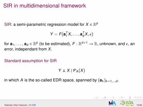
SIR in multidimensional framework
SIR: a semi-parametric regression model for X ∈ Rp
Y = F(aT1 X , . . . , aT
d X , ε)
for a1, . . . , ad ∈ Rp (to be estimated), F : Rd+1 → R, unknown, and ε, an
error, independant from X .
Standard assumption for SIR
Y y X | PA (X)
in which A is the so-called EDR space, spanned by (ak )k=1,...,d .
Nathalie Villa-Vialaneix | IS-SIR 10/26

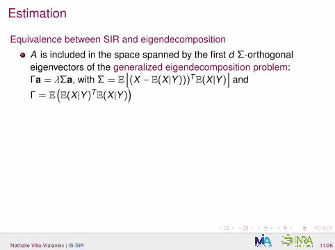
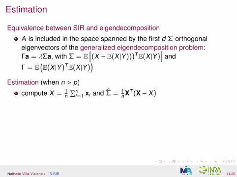
Estimation
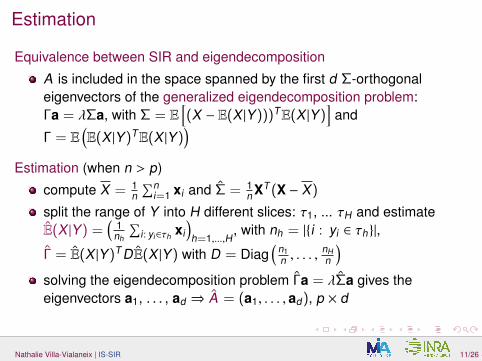
Equivalence between SIR and eigendecomposition
A is included in the space spanned by the first d Σ-orthogonaleigenvectors of the generalized eigendecomposition problem:Γa = λΣa, with Σ = E
[(X − E(X |Y)))TE(X |Y)
]and
Γ = E(E(X |Y)TE(X |Y)
)Estimation (when n > p)
compute X = 1n∑n
i=1 xi and Σ = 1n XT (X − X)
split the range of Y into H different slices: τ1, ... τH and estimateE(X |Y) =
(1nh
∑i: yi∈τh
xi
)h=1,...,H
, with nh = |{i : yi ∈ τh}|,
Γ = E(X |Y)T DE(X |Y) with D = Diag(
n1n , . . . ,
nHn
)solving the eigendecomposition problem Γa = λΣa gives theeigenvectors a1, . . . , ad ⇒ A = (a1, . . . , ad), p × d
Nathalie Villa-Vialaneix | IS-SIR 11/26
Estimation
Equivalence between SIR and eigendecomposition
A is included in the space spanned by the first d Σ-orthogonaleigenvectors of the generalized eigendecomposition problem:Γa = λΣa, with Σ = E
[(X − E(X |Y)))TE(X |Y)
]and
Γ = E(E(X |Y)TE(X |Y)
)
Estimation (when n > p)
compute X = 1n∑n
i=1 xi and Σ = 1n XT (X − X)
split the range of Y into H different slices: τ1, ... τH and estimateE(X |Y) =
(1nh
∑i: yi∈τh
xi
)h=1,...,H
, with nh = |{i : yi ∈ τh}|,
Γ = E(X |Y)T DE(X |Y) with D = Diag(
n1n , . . . ,
nHn
)solving the eigendecomposition problem Γa = λΣa gives theeigenvectors a1, . . . , ad ⇒ A = (a1, . . . , ad), p × d
Nathalie Villa-Vialaneix | IS-SIR 11/26
Estimation
Equivalence between SIR and eigendecomposition
A is included in the space spanned by the first d Σ-orthogonaleigenvectors of the generalized eigendecomposition problem:Γa = λΣa, with Σ = E
[(X − E(X |Y)))TE(X |Y)
]and
Γ = E(E(X |Y)TE(X |Y)
)Estimation (when n > p)
compute X = 1n∑n
i=1 xi and Σ = 1n XT (X − X)
split the range of Y into H different slices: τ1, ... τH and estimateE(X |Y) =
(1nh
∑i: yi∈τh
xi
)h=1,...,H
, with nh = |{i : yi ∈ τh}|,
Γ = E(X |Y)T DE(X |Y) with D = Diag(
n1n , . . . ,
nHn
)solving the eigendecomposition problem Γa = λΣa gives theeigenvectors a1, . . . , ad ⇒ A = (a1, . . . , ad), p × d
Nathalie Villa-Vialaneix | IS-SIR 11/26

Estimation
Equivalence between SIR and eigendecomposition
A is included in the space spanned by the first d Σ-orthogonaleigenvectors of the generalized eigendecomposition problem:Γa = λΣa, with Σ = E
[(X − E(X |Y)))TE(X |Y)
]and
Γ = E(E(X |Y)TE(X |Y)
)Estimation (when n > p)
compute X = 1n∑n
i=1 xi and Σ = 1n XT (X − X)
split the range of Y into H different slices: τ1, ... τH and estimateE(X |Y) =
(1nh
∑i: yi∈τh
xi
)h=1,...,H
, with nh = |{i : yi ∈ τh}|,
Γ = E(X |Y)T DE(X |Y) with D = Diag(
n1n , . . . ,
nHn
)
solving the eigendecomposition problem Γa = λΣa gives theeigenvectors a1, . . . , ad ⇒ A = (a1, . . . , ad), p × d
Nathalie Villa-Vialaneix | IS-SIR 11/26
Estimation
Equivalence between SIR and eigendecomposition
A is included in the space spanned by the first d Σ-orthogonaleigenvectors of the generalized eigendecomposition problem:Γa = λΣa, with Σ = E
[(X − E(X |Y)))TE(X |Y)
]and
Γ = E(E(X |Y)TE(X |Y)
)Estimation (when n > p)
compute X = 1n∑n
i=1 xi and Σ = 1n XT (X − X)
split the range of Y into H different slices: τ1, ... τH and estimateE(X |Y) =
(1nh
∑i: yi∈τh
xi
)h=1,...,H
, with nh = |{i : yi ∈ τh}|,
Γ = E(X |Y)T DE(X |Y) with D = Diag(
n1n , . . . ,
nHn
)solving the eigendecomposition problem Γa = λΣa gives theeigenvectors a1, . . . , ad ⇒ A = (a1, . . . , ad), p × d
Nathalie Villa-Vialaneix | IS-SIR 11/26

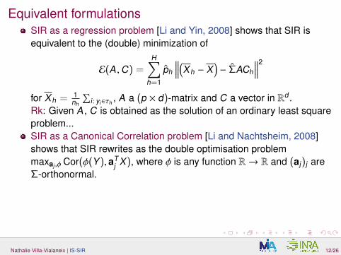
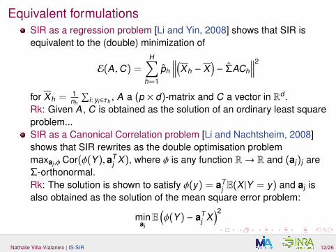
Equivalent formulationsSIR as a regression problem [Li and Yin, 2008] shows that SIR isequivalent to the (double) minimization of
E(A ,C) =H∑
h=1
ph
∥∥∥∥(Xh − X)− ΣACh
∥∥∥∥2
for Xh = 1nh
∑i: yi∈τh
, A a (p × d)-matrix and C a vector in Rd .
Rk: Given A , C is obtained as the solution of an ordinary least squareproblem...SIR as a Canonical Correlation problem [Li and Nachtsheim, 2008]shows that SIR rewrites as the double optimisation problemmaxaj ,φ Cor(φ(Y), aT
j X), where φ is any function R→ R and (aj)j areΣ-orthonormal.
Rk: The solution is shown to satisfy φ(y) = aTj E(X |Y = y) and aj is
also obtained as the solution of the mean square error problem:
minajE
(φ(Y) − aT
j X)2
Nathalie Villa-Vialaneix | IS-SIR 12/26

Equivalent formulationsSIR as a regression problem [Li and Yin, 2008] shows that SIR isequivalent to the (double) minimization of
E(A ,C) =H∑
h=1
ph
∥∥∥∥(Xh − X)− ΣACh
∥∥∥∥2
for Xh = 1nh
∑i: yi∈τh
, A a (p × d)-matrix and C a vector in Rd .Rk: Given A , C is obtained as the solution of an ordinary least squareproblem...
SIR as a Canonical Correlation problem [Li and Nachtsheim, 2008]shows that SIR rewrites as the double optimisation problemmaxaj ,φ Cor(φ(Y), aT
j X), where φ is any function R→ R and (aj)j areΣ-orthonormal.
Rk: The solution is shown to satisfy φ(y) = aTj E(X |Y = y) and aj is
also obtained as the solution of the mean square error problem:
minajE
(φ(Y) − aT
j X)2
Nathalie Villa-Vialaneix | IS-SIR 12/26
Equivalent formulationsSIR as a regression problem [Li and Yin, 2008] shows that SIR isequivalent to the (double) minimization of
E(A ,C) =H∑
h=1
ph
∥∥∥∥(Xh − X)− ΣACh
∥∥∥∥2
for Xh = 1nh
∑i: yi∈τh
, A a (p × d)-matrix and C a vector in Rd .Rk: Given A , C is obtained as the solution of an ordinary least squareproblem...SIR as a Canonical Correlation problem [Li and Nachtsheim, 2008]shows that SIR rewrites as the double optimisation problemmaxaj ,φ Cor(φ(Y), aT
j X), where φ is any function R→ R and (aj)j areΣ-orthonormal.Rk: The solution is shown to satisfy φ(y) = aT
j E(X |Y = y) and aj isalso obtained as the solution of the mean square error problem:
minajE
(φ(Y) − aT
j X)2
Nathalie Villa-Vialaneix | IS-SIR 12/26

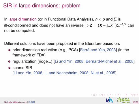
SIR in large dimensions: problem
In large dimension (or in Functional Data Analysis), n < p and Σ is
ill-conditionned and does not have an inverse⇒ Z = (X − InXT
)Σ−1/2 cannot be computed.
Different solutions have been proposed in the litterature based on:
prior dimension reduction (e.g., PCA) [Ferré and Yao, 2003] (in theframework of FDA)
regularization (ridge...) [Li and Yin, 2008, Bernard-Michel et al., 2008]
sparse SIR[Li and Yin, 2008, Li and Nachtsheim, 2008, Ni et al., 2005]
Nathalie Villa-Vialaneix | IS-SIR 13/26

SIR in large dimensions: ridge penalty / L2-regularizationof Σ
Following [Li and Yin, 2008] which shows that SIR is equivalent to theminimization of
E2(A ,C) =H∑
h=1
ph
∥∥∥∥(Xh − X)− ΣACh
∥∥∥∥2
+µ2
H∑h=1
ph‖ACh‖2
,
[Bernard-Michel et al., 2008] propose to penalize by a ridge penalty in ahigh dimensional setting.
They also show that this problem is equivalent to finding the eigenvectorsof the generalized eigenvalue problem
Γa = λ(Σ + µ2Ip
)a.
Nathalie Villa-Vialaneix | IS-SIR 14/26

SIR in large dimensions: ridge penalty / L2-regularizationof Σ
Following [Li and Yin, 2008] which shows that SIR is equivalent to theminimization of
E2(A ,C) =H∑
h=1
ph
∥∥∥∥(Xh − X)− ΣACh
∥∥∥∥2+µ2
H∑h=1
ph‖ACh‖2,
[Bernard-Michel et al., 2008] propose to penalize by a ridge penalty in ahigh dimensional setting.
They also show that this problem is equivalent to finding the eigenvectorsof the generalized eigenvalue problem
Γa = λ(Σ + µ2Ip
)a.
Nathalie Villa-Vialaneix | IS-SIR 14/26

SIR in large dimensions: sparse versions
Specific issue to introduce sparsity in SIRsparsity on a multiple-index model. Most authors use shrinkageapproaches.
First version: sparse penalization of the ridge solutionIf (A , C) are the solutions of the ridge SIR as described in the previousslide, [Ni et al., 2005, Li and Yin, 2008] propose to shrink this solution byminimizing
Es,1(α) =H∑
h=1
ph
∥∥∥∥(Xh − X)− ΣDiag(α)A Ch
∥∥∥∥2+ µ1‖α‖L1
(regression formulation of SIR)
Nathalie Villa-Vialaneix | IS-SIR 15/26

SIR in large dimensions: sparse versions
Specific issue to introduce sparsity in SIRsparsity on a multiple-index model. Most authors use shrinkageapproaches.
Second version: [Li and Nachtsheim, 2008] derive the sparse optimizationproblem from the correlation formulation of SIR:
minas
j
n∑i=1
[Paj (X |yi) − (as
j )T xi
]2+ µ1,j‖as
j ‖L1 ,
in which Paj is the projection of E(X |Y = yi) = Xh onto the space spannedby the solution of the ridge problem.
Nathalie Villa-Vialaneix | IS-SIR 15/26

Characteristics of the different approaches and possibleextensions
[Li and Yin, 2008] [Li and Nachtsheim, 2008]
sparsity on shrinkage coefficients estimatesnb optimization pb 1 dsparsity common to all dims specific to each dim
Extension to block-sparse SIR (like in PCA)?
Nathalie Villa-Vialaneix | IS-SIR 16/26

Sommaire
1 Background and motivation
2 Presentation of SIR
3 Our proposal
4 Simulations
Nathalie Villa-Vialaneix | IS-SIR 17/26

IS-SIR: a two step approachBackground: Back to the functional setting, we suppose that t1, ..., tp aresplit into D intervals I1, ..., ID .
First step: Solve the ridge problem on the digitized functions (viewed ashigh dimensional vectors) to obtain A and C:
minA ,C
H∑h=1
ph
∥∥∥∥(Xh − X)− ΣACh
∥∥∥∥2+ µ2
H∑h=1
ph‖ACh‖2
Second step: Sparse shrinkage using the intervals. IfPA (E(X |Y = yi)) = (Xh − X)T A for h st yi ∈ τh and if Pi = (P1
i , . . . ,Pdi )T
and Pj = (Pj1, . . . ,P
jn)T , we solve:
arg minα∈RD
d∑j=1
‖Pj − (X∆(aj))α‖2 + µ1‖α‖L1
with ∆(aj) the (p × D)-matrix such that ∆kl(aj) = ajl if tl ∈ Ik and 0otherwise.
Nathalie Villa-Vialaneix | IS-SIR 18/26

IS-SIR: a two step approachBackground: Back to the functional setting, we suppose that t1, ..., tp aresplit into D intervals I1, ..., ID .First step: Solve the ridge problem on the digitized functions (viewed ashigh dimensional vectors) to obtain A and C:
minA ,C
H∑h=1
ph
∥∥∥∥(Xh − X)− ΣACh
∥∥∥∥2+ µ2
H∑h=1
ph‖ACh‖2
Second step: Sparse shrinkage using the intervals. IfPA (E(X |Y = yi)) = (Xh − X)T A for h st yi ∈ τh and if Pi = (P1
i , . . . ,Pdi )T
and Pj = (Pj1, . . . ,P
jn)T , we solve:
arg minα∈RD
d∑j=1
‖Pj − (X∆(aj))α‖2 + µ1‖α‖L1
with ∆(aj) the (p × D)-matrix such that ∆kl(aj) = ajl if tl ∈ Ik and 0otherwise.
Nathalie Villa-Vialaneix | IS-SIR 18/26

IS-SIR: Characteristics
uses the approach based on the correlation formulation (because thedimensionality of the optimization problem is smaller);
uses a shrinkage approach and optimizes shrinkage coefficients in asingle optimization problem;
handles functional setting by penalizing entire intervals and not justisolated points.
Nathalie Villa-Vialaneix | IS-SIR 19/26

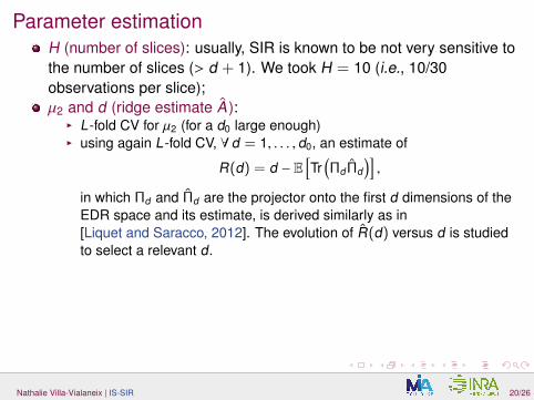
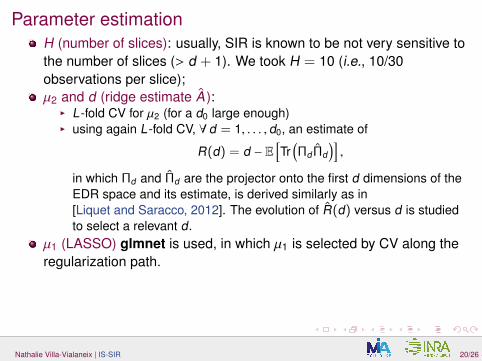
Parameter estimationH (number of slices): usually, SIR is known to be not very sensitive tothe number of slices (> d + 1). We took H = 10 (i.e., 10/30observations per slice);
µ2 and d (ridge estimate A ):I L -fold CV for µ2 (for a d0 large enough)
I using again L -fold CV, ∀ d = 1, . . . , d0, an estimate of
R(d) = d − E[Tr
(ΠdΠd
)],
in which Πd and Πd are the projector onto the first d dimensions of theEDR space and its estimate, is derived similarly as in[Liquet and Saracco, 2012]. The evolution of R(d) versus d is studiedto select a relevant d.
µ1 (LASSO) glmnet is used, in which µ1 is selected by CV along theregularization path.
Nathalie Villa-Vialaneix | IS-SIR 20/26

Parameter estimationH (number of slices): usually, SIR is known to be not very sensitive tothe number of slices (> d + 1). We took H = 10 (i.e., 10/30observations per slice);µ2 and d (ridge estimate A ):
I L -fold CV for µ2 (for a d0 large enough) Note that GCV as described in[Li and Yin, 2008] can not be used since the current version of the L2
penalty involves the use of an estimate of Σ−1.
I using again L -fold CV, ∀ d = 1, . . . , d0, an estimate of
R(d) = d − E[Tr
(ΠdΠd
)],
in which Πd and Πd are the projector onto the first d dimensions of theEDR space and its estimate, is derived similarly as in[Liquet and Saracco, 2012]. The evolution of R(d) versus d is studiedto select a relevant d.
µ1 (LASSO) glmnet is used, in which µ1 is selected by CV along theregularization path.
Nathalie Villa-Vialaneix | IS-SIR 20/26
Parameter estimationH (number of slices): usually, SIR is known to be not very sensitive tothe number of slices (> d + 1). We took H = 10 (i.e., 10/30observations per slice);µ2 and d (ridge estimate A ):
I L -fold CV for µ2 (for a d0 large enough)I using again L -fold CV, ∀ d = 1, . . . , d0, an estimate of
R(d) = d − E[Tr
(ΠdΠd
)],
in which Πd and Πd are the projector onto the first d dimensions of theEDR space and its estimate, is derived similarly as in[Liquet and Saracco, 2012]. The evolution of R(d) versus d is studiedto select a relevant d.
µ1 (LASSO) glmnet is used, in which µ1 is selected by CV along theregularization path.
Nathalie Villa-Vialaneix | IS-SIR 20/26

An automatic approach to define intervals1 Initial state: ∀ k = 1, . . . , p, τk = {tk }
2 Iterate
I define: D− (“strong zeros”) and D+ (“strong non zeros”)
Final solution: Minimize GCVD over D.
Nathalie Villa-Vialaneix | IS-SIR 21/26
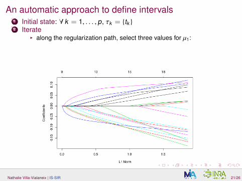
An automatic approach to define intervals1 Initial state: ∀ k = 1, . . . , p, τk = {tk }2 Iterate
I along the regularization path, select three values for µ1:
P% of thecoefficients are zero, P% of the coefficients are non zero, best GCV.define: D− (“strong zeros”) and D+ (“strong non zeros”)
Final solution: Minimize GCVD over D.
Nathalie Villa-Vialaneix | IS-SIR 21/26
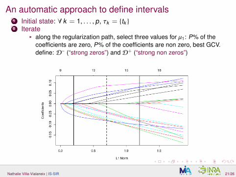
An automatic approach to define intervals1 Initial state: ∀ k = 1, . . . , p, τk = {tk }2 Iterate
I along the regularization path, select three values for µ1: P% of thecoefficients are zero, P% of the coefficients are non zero, best GCV.define: D− (“strong zeros”) and D+ (“strong non zeros”)
Final solution: Minimize GCVD over D.
Nathalie Villa-Vialaneix | IS-SIR 21/26

An automatic approach to define intervals1 Initial state: ∀ k = 1, . . . , p, τk = {tk }2 Iterate
I define: D− (“strong zeros”) and D+ (“strong non zeros”)I merge consecutive “strong zeros” (or “strong non zeros”) or “strong
zeros” (resp. “strong non zeros”) separated by a few numbers ofintervals which are of undetermined type.
Until no more iterations can be performed.
Final solution: Minimize GCVD over D.
Nathalie Villa-Vialaneix | IS-SIR 21/26

An automatic approach to define intervals1 Initial state: ∀ k = 1, . . . , p, τk = {tk }2 Iterate
I define: D− (“strong zeros”) and D+ (“strong non zeros”)I merge consecutive “strong zeros” (or “strong non zeros”) or “strong
zeros” (resp. “strong non zeros”) separated by a few numbers ofintervals which are of undetermined type.
Until no more iterations can be performed.3 Output: Collection of models (first with p intervals, last with 1),M∗D
(optimal for GCV) and corresponding GCVD versus D (number ofintervals).
Final solution: Minimize GCVD over D.
Nathalie Villa-Vialaneix | IS-SIR 21/26

Sommaire
1 Background and motivation
2 Presentation of SIR
3 Our proposal
4 Simulations
Nathalie Villa-Vialaneix | IS-SIR 22/26
Simulation framework
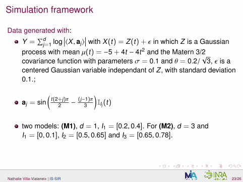
Data generated with:
Y =∑d
j=1 log∣∣∣〈X , aj〉
∣∣∣ with X(t) = Z(t) + ε in which Z is a Gaussianprocess with mean µ(t) = −5 + 4t − 4t2 and the Matern 3/2covariance function with parameters σ = 0.1 and θ = 0.2/
√3, ε is a
centered Gaussian variable independant of Z , with standard deviation0.1.;
aj = sin(
t(2+j)π2 −
(j−1)π3
)IIj (t)
two models: (M1), d = 1, I1 = [0.2, 0.4]. For (M2), d = 3 andI1 = [0, 0.1], I2 = [0.5, 0.65] and I3 = [0.65, 0.78].
Nathalie Villa-Vialaneix | IS-SIR 23/26

Simulation framework
Nathalie Villa-Vialaneix | IS-SIR 23/26

Simulation framework
Nathalie Villa-Vialaneix | IS-SIR 23/26

Ridge step (model M1)
Selection of µ2: µ2 = 1
Nathalie Villa-Vialaneix | IS-SIR 24/26

Ridge step (model M1)
Selection of d: d = 1
Nathalie Villa-Vialaneix | IS-SIR 24/26

Definition of the intervalsD = 200 (initial state)
0.2 0.4 0.6 0.8 1.0
0.0
0.2
0.4
0.6
0.8
a 1
●
●
●
●
●●●
●
●●●
●
●
●
●
●
●
●
●
●
●
●●
●
●
●
●
●
●
●
●
●●
●
●
●
0 50 100 150 200
0.01
90.
020
0.02
10.
022
0.02
3
Number of intervals
CV
err
or
Nathalie Villa-Vialaneix | IS-SIR 25/26
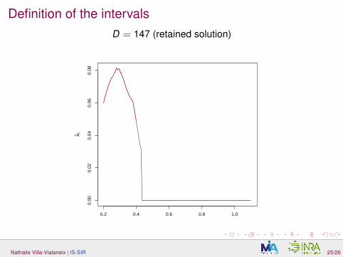
Definition of the intervalsD = 147 (retained solution)
0.2 0.4 0.6 0.8 1.0
0.00
0.02
0.04
0.06
0.08
a 1
●
●
●
●
●●●
●
●●●
●
●
●
●
●
●
●
●
●
●
●●
●
●
●
●
●
●
●
●
●●
●
●
●
0 50 100 150 200
0.01
90.
020
0.02
10.
022
0.02
3
Number of intervals
CV
err
or
Nathalie Villa-Vialaneix | IS-SIR 25/26
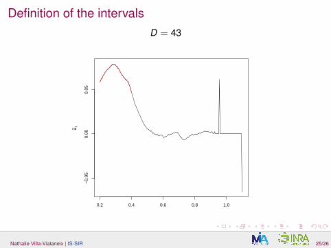
Definition of the intervalsD = 43
0.2 0.4 0.6 0.8 1.0
−0.
050.
000.
05
a 1
●
●
●
●
●●●
●
●●●
●
●
●
●
●
●
●
●
●
●
●●
●
●
●
●
●
●
●
●
●●
●
●
●
0 50 100 150 200
0.01
90.
020
0.02
10.
022
0.02
3
Number of intervals
CV
err
or
Nathalie Villa-Vialaneix | IS-SIR 25/26

Definition of the intervalsD = 5
0.2 0.4 0.6 0.8 1.0
−0.
04−
0.02
0.00
0.02
0.04
0.06
0.08
a 1
●
●
●
●
●●●
●
●●●
●
●
●
●
●
●
●
●
●
●
●●
●
●
●
●
●
●
●
●
●●
●
●
●
0 50 100 150 200
0.01
90.
020
0.02
10.
022
0.02
3
Number of intervals
CV
err
or
Nathalie Villa-Vialaneix | IS-SIR 25/26

Definition of the intervals
●
●
●
●
●●●
●
●●●
●
●
●
●
●
●
●
●
●
●
●●
●
●
●
●
●
●
●
●
●●
●
●
●
0 50 100 150 200
0.01
90.
020
0.02
10.
022
0.02
3
Number of intervals
CV
err
or
Nathalie Villa-Vialaneix | IS-SIR 25/26

Conclusion
IS-SIR:
sparse dimension reduction model adapted to functional framework;
fully automated definition of relevant intervals in the range of thepredictors
Perspective:
application to real data
block-wise sparse SIR?
Nathalie Villa-Vialaneix | IS-SIR 26/26

Conclusion
IS-SIR:
sparse dimension reduction model adapted to functional framework;
fully automated definition of relevant intervals in the range of thepredictors
Perspective:
application to real data
block-wise sparse SIR?
Nathalie Villa-Vialaneix | IS-SIR 26/26

Aneiros, G. and Vieu, P. (2014).Variable in infinite-dimensional problems.Statistics and Probability Letters, 94:12–20.
Bernard-Michel, C., Gardes, L., and Girard, S. (2008).A note on sliced inverse regression with regularizations.Biometrics, 64(3):982–986.
Casadebaig, P., Guilioni, L., Lecoeur, J., Christophe, A., Champolivier, L., and Debaeke, P. (2011).SUNFLO, a model to simulate genotype-specific performance of the sunflower crop in contrasting environments.Agricultural and Forest Meteorology, 151(2):163–178.
Ferraty, F., Hall, P., and Vieu, P. (2010).Most-predictive design points for functiona data predictors.Biometrika, 97(4):807–824.
Ferré, L. and Yao, A. (2003).Functional sliced inverse regression analysis.Statistics, 37(6):475–488.
Fraiman, R., Gimenez, Y., and Svarc, M. (2015).Feature selection for functional data.Journal of Multivariate Analysis.In Press.
Gregorutti, B., Michel, B., and Saint-Pierre, P. (2015).Grouped variable importance with random forests and application to multiple functional data analysis.Computational Statistics and Data Analysis, 90:15–35.
James, G., Wang, J., and Zhu, J. (2009).Functional linear regression that’s interpretable.Annals of Statistics, 37(5A):2083–2108.
Li, L. and Nachtsheim, C. (2008).
Nathalie Villa-Vialaneix | IS-SIR 26/26

Sparse sliced inverse regression.Technometrics, 48(4):503–510.
Li, L. and Yin, X. (2008).Sliced inverse regression with regularizations.Biometrics, 64:124–131.
Liquet, B. and Saracco, J. (2012).A graphical tool for selecting the number of slices and the dimension of the model in SIR and SAVE approches.Computational Statistics, 27(1):103–125.
Matsui, H. and Konishi, S. (2011).Variable selection for functional regression models via the l1 regularization.Computational Statistics and Data Analysis, 55(12):3304–3310.
Ni, L., Cook, D., and Tsai, C. (2005).A note on shrinkage sliced inverse regression.Biometrika, 92(1):242–247.
Nathalie Villa-Vialaneix | IS-SIR 26/26