ICAM: Interpretable Classification via DisentangledRepresentations and Feature Attribution Mapping

Cher BassKings College London

London, UK, WC2R 2LScher.bass@kcl.ac.uk

Mariana da SilvaKings College London

London, UK, WC2R 2LS

Carole SudreKings College London

London, UK, WC2R 2LS

Petru-Daniel TudosiuKings College London

London, UK, WC2R 2LS

Stephen M. SmithUniversity of Oxford

Oxford, UK, OX1 2JD

Emma C. RobinsonKings College London

London, UK, WC2R 2LSemma.robinson@kcl.ac.uk

Abstract

Feature attribution (FA), or the assignment of class-relevance to different locationsin an image, is important for many classification problems but is particularly crucialwithin the neuroscience domain, where accurate mechanistic models of behaviours,or disease, require knowledge of all features discriminative of a trait. At the sametime, predicting class relevance from brain images is challenging as phenotypesare typically heterogeneous, and changes occur against a background of significantnatural variation. Here, we present a novel framework for creating class specificFA maps through image-to-image translation. We propose the use of a VAE-GANto explicitly disentangle class relevance from background features for improvedinterpretability properties, which results in meaningful FA maps. We validate ourmethod on 2D and 3D brain image datasets of dementia (ADNI dataset), ageing(UK Biobank), and (simulated) lesion detection. We show that FA maps generatedby our method outperform baseline FA methods when validated against groundtruth. More significantly, our approach is the first to use latent space sampling tosupport exploration of phenotype variation.

1 Introduction

Brain images present a significant resource in the development of mechanistic models of behaviour andneurological/psychiatric disease as they reflect measurable neuroanatomical traits that are heritable,present in unaffected siblings and detectable prior to disease onset [10]. Nevertheless, for complexdisorders, features of disease remain subtle, variable [21, 38] and occur against a back-drop ofsignificant natural variation in shape and appearance [16, 27].

Traditional approaches for brain image analysis compare data in a global average template space,estimated via smooth (and ideally diffeomorphic) deformations [2, 11, 12, 14, 16, 37]. This, however,typically ignores cortical heterogeneity and may smooth out sources of variation [11, 16] in wayswhich limit interpretation [7]. Tools are still required to distinguish between features of populationvariability and specific discriminative phenotypic features.

Deep learning is state-of-the-art for many image processing tasks [17] and has shown strong promisefor brain imaging applications such as healthy tissue and lesion segmentation [8, 13, 25, 36]. However,there is growing need for greater accountability of networks, especially within the medical domain.Several approaches for feature attribution (FA) [3, 30, 33, 40, 43] have been proposed which return

34th Conference on Neural Information Processing Systems (NeurIPS 2020), Vancouver, Canada.

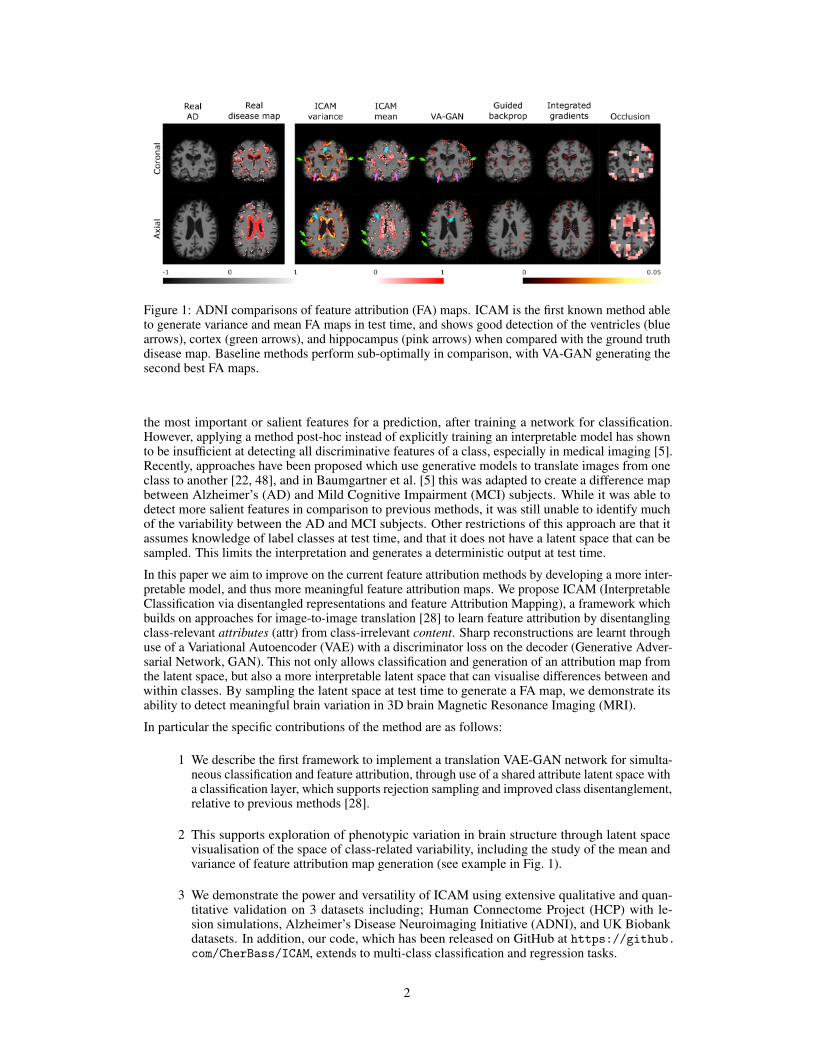
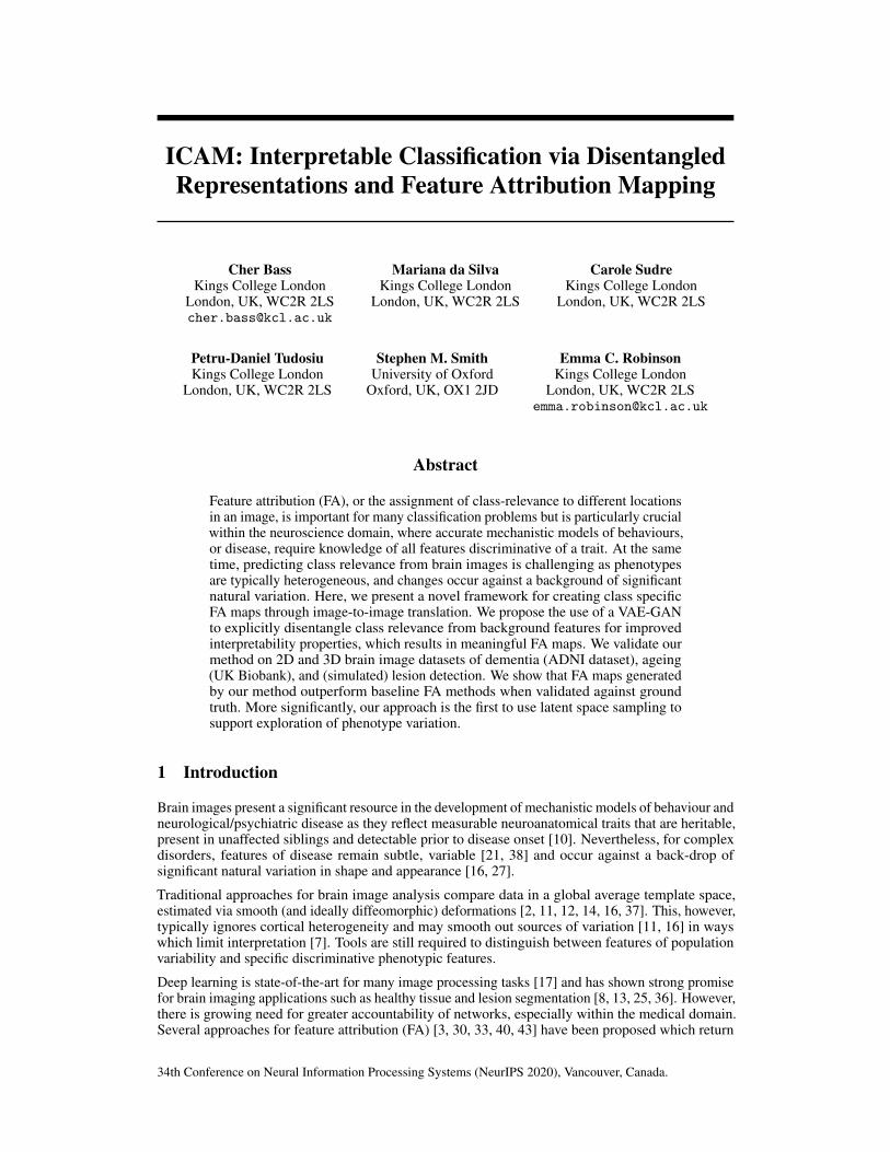
Figure 1: ADNI comparisons of feature attribution (FA) maps. ICAM is the first known method ableto generate variance and mean FA maps in test time, and shows good detection of the ventricles (bluearrows), cortex (green arrows), and hippocampus (pink arrows) when compared with the ground truthdisease map. Baseline methods perform sub-optimally in comparison, with VA-GAN generating thesecond best FA maps.

the most important or salient features for a prediction, after training a network for classification.However, applying a method post-hoc instead of explicitly training an interpretable model has shownto be insufficient at detecting all discriminative features of a class, especially in medical imaging [5].Recently, approaches have been proposed which use generative models to translate images from oneclass to another [22, 48], and in Baumgartner et al. [5] this was adapted to create a difference mapbetween Alzheimer’s (AD) and Mild Cognitive Impairment (MCI) subjects. While it was able todetect more salient features in comparison to previous methods, it was still unable to identify muchof the variability between the AD and MCI subjects. Other restrictions of this approach are that itassumes knowledge of label classes at test time, and that it does not have a latent space that can besampled. This limits the interpretation and generates a deterministic output at test time.

In this paper we aim to improve on the current feature attribution methods by developing a more inter-pretable model, and thus more meaningful feature attribution maps. We propose ICAM (InterpretableClassification via disentangled representations and feature Attribution Mapping), a framework whichbuilds on approaches for image-to-image translation [28] to learn feature attribution by disentanglingclass-relevant attributes (attr) from class-irrelevant content. Sharp reconstructions are learnt throughuse of a Variational Autoencoder (VAE) with a discriminator loss on the decoder (Generative Adver-sarial Network, GAN). This not only allows classification and generation of an attribution map fromthe latent space, but also a more interpretable latent space that can visualise differences between andwithin classes. By sampling the latent space at test time to generate a FA map, we demonstrate itsability to detect meaningful brain variation in 3D brain Magnetic Resonance Imaging (MRI).

In particular the specific contributions of the method are as follows:

1 We describe the first framework to implement a translation VAE-GAN network for simulta-neous classification and feature attribution, through use of a shared attribute latent space witha classification layer, which supports rejection sampling and improved class disentanglement,relative to previous methods [28].

2 This supports exploration of phenotypic variation in brain structure through latent spacevisualisation of the space of class-related variability, including the study of the mean andvariance of feature attribution map generation (see example in Fig. 1).

3 We demonstrate the power and versatility of ICAM using extensive qualitative and quan-titative validation on 3 datasets including; Human Connectome Project (HCP) with le-sion simulations, Alzheimer’s Disease Neuroimaging Initiative (ADNI), and UK Biobankdatasets. In addition, our code, which has been released on GitHub at https://github.com/CherBass/ICAM, extends to multi-class classification and regression tasks.

2

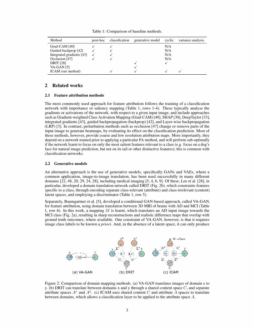
Table 1: Comparison of baseline methods.

Method post-hoc classification generative model cyclic variance analysis

Grad-CAM [40] X X N/AGuided backprop [42] X X N/AIntegrated gradients [43] X X N/AOcclusion [47] X X N/ADRIT [28] X XVA-GAN [5] XICAM (our method) X X X X

2 Related works

2.1 Feature attribution methods

The most commonly used approach for feature attribution follows the training of a classificationnetwork with importance or saliency mapping (Table 1, rows 1-4). These typically analyse thegradients or activations of the network, with respect to a given input image, and include approachessuch as Gradient-weighted Class Activation Mapping (Grad-CAM) [40], SHAP [30], DeepTaylor [33],integrated gradients [43], guided backpropagation (backprop) [42], and Layer-wise backpropagation(LRP) [3]. In contrast, perturbation methods such as occlusion [47] change or remove parts of theinput image to generate heatmaps, by evaluating its effect on the classification prediction. Most ofthese methods, however, provide coarse and low resolution attribution maps. More importantly, theydepend on a network trained prior to applying a particular FA method, and will perform sub-optimallyif the network learnt to focus on only the most salient features relevant to a class (e.g. focus on a dog’sface for natural image prediction, but not on its tail or other distinctive features); this is common withclassification networks.

2.2 Generative models

An alternative approach is the use of generative models, specifically GANs and VAEs, where acommon application, image-to-image translation, has been used successfully in many differentdomains [22, 48, 20, 29, 24, 28], including medical imaging [5, 4, 6, 9]. Of these, Lee et al. [28], inparticular, developed a domain translation network called DRIT (Fig. 2b), which constraints featuresspecific to a class, through encoding separate class-relevant (attribute) and class-irrelevant (content)latent spaces, and employing a discriminator (Table 1, row 5).

Separately, Baumgartner et al. [5], developed a conditional GAN-based approach, called VA-GAN,for feature attribution, using domain translation between 3D MRI of brains with AD and MCI (Table1, row 6). In this work, a mapping M is learnt, which translates an AD input image towards theMCI class (Fig. 2a), resulting in sharp reconstructions and realistic difference maps that overlap withground truth outcomes, where available. One constraint of VA-GAN, however, is that it requiresimage class labels to be known a priori. And, in the absence of a latent space, it can only produce

Figure 2: Comparison of domain mapping methods. (a) VA-GAN translates images of domain x toy. (b) DRIT can translate between domains x and y through a shared content space C, and separateattribute spaces Ax and Ay. (c) ICAM uses shared content C and attribute A spaces to translatebetween domains, which allows a classification layer to be applied to the attribute space A.

3

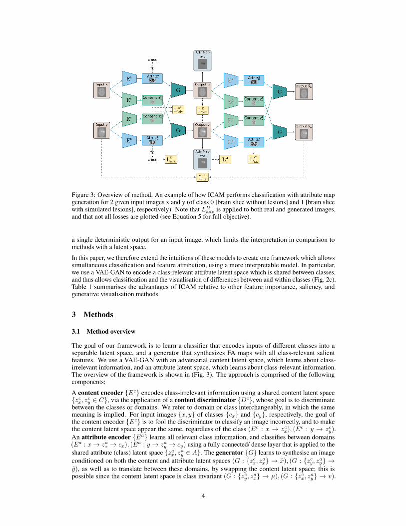
Figure 3: Overview of method. An example of how ICAM performs classification with attribute mapgeneration for 2 given input images x and y (of class 0 [brain slice without lesions] and 1 [brain slicewith simulated lesions], respectively). Note that LD

adv is applied to both real and generated images,and that not all losses are plotted (see Equation 5 for full objective).

a single deterministic output for an input image, which limits the interpretation in comparison tomethods with a latent space.

In this paper, we therefore extend the intuitions of these models to create one framework which allowssimultaneous classification and feature attribution, using a more interpretable model. In particular,we use a VAE-GAN to encode a class-relevant attribute latent space which is shared between classes,and thus allows classification and the visualisation of differences between and within classes (Fig. 2c).Table 1 summarises the advantages of ICAM relative to other feature importance, saliency, andgenerative visualisation methods.

3 Methods

3.1 Method overview

The goal of our framework is to learn a classifier that encodes inputs of different classes into aseparable latent space, and a generator that synthesizes FA maps with all class-relevant salientfeatures. We use a VAE-GAN with an adversarial content latent space, which learns about class-irrelevant information, and an attribute latent space, which learns about class-relevant information.The overview of the framework is shown in (Fig. 3). The approach is comprised of the followingcomponents:

A content encoder {Ec} encodes class-irrelevant information using a shared content latent space{zcx, zcy ∈ C}, via the application of a content discriminator {Dc}, whose goal is to discriminatebetween the classes or domains. We refer to domain or class interchangeably, in which the samemeaning is implied. For input images {x, y} of classes {cx} and {cy}, respectively, the goal ofthe content encoder {Ec} is to fool the discriminator to classify an image incorrectly, and to makethe content latent space appear the same, regardless of the class (Ec : x → zcx), (E

c : y → zcy).An attribute encoder {Ea} learns all relevant class information, and classifies between domains(Ea : x→ zax → cx), (E

a : y → zay → cy) using a fully connected/ dense layer that is applied to theshared attribute (class) latent space {zax, zay ∈ A}. The generator {G} learns to synthesise an imageconditioned on both the content and attribute latent spaces (G : {zcx, zax} → x), (G : {zcy, zay} →y), as well as to translate between these domains, by swapping the content latent space; this ispossible since the content latent space is class invariant (G : {zcy, zax} → µ), (G : {zcx, zay} → v).

4

Translating the domains enables the visualisation of differences between the two classes, using afeature attribution map ({Mx = v − x}, {My = µ − y}). Finally, the domain discriminator{D} learns to distinguish between generated and real images, and to classify the two domains, whichgives a clearer training signal for the generator.

Our network architectures uses 2D or 3D convolutional layers (kernel size = 3 or 4), ResNet layersincluding basic, down, and deconvolutional blocks with instance normalisation. A key feature of thenetwork architecture is encoding the latent space as a 2D or 3D vector, instead of a 1D vector as iscommonly seen in VAEs. For example, for a latent space size of 80, a 1D vector = [80], 2D vector =[8,10]. This allows the network to encode spatial, and shape related information in the latent space,which is important in brain imaging. A detailed diagram of our encoder-generator architecture (for a3D input) is shown in supplementary section A.1.

3.2 Content and attribute spaces

Our approach disentangles the two image domains into a shared content space {C}, and attributespace {A}. The content latent space aims to encode class irrelevant information: features commonto both domains (e.g. location of structures, and folds of the brain). The attribute latent spaceaims to map the remaining domain-specific information onto shared latent space {A}, thus enablingclassification using all salient features, and cross-domain translation.

Content loss. To achieve domain disentanglement, we employ a common content encoder for bothdomains ({Ec : x → C}, {Ec : y → C}). The content latent space {C} is fed into a contentdiscriminator, {Dc}, which outputs the image class probability. The content discriminator {Dc}aids the representation to be disentangled, by aiming to distinguish between domains (classes) ofthe encoded latent spaces {zcx} and {zcy}. Inversely, the content encoder {Ec} aims to encode arepresentation whose domain cannot be distinguished by the content discriminator, and thus forcesthe representation to be mapped to the same space {C}, similarly to Lee et al. [28].

This class adversarial content loss can be expressed as:

LDc

adv = Ezcx[logDc(Ec(x)) + log(1−Dc(Ec(x)))]

+Ezcy[logDc(Ec(y)) + log(1−Dc(Ec(y)))].

(1)

An L2 regularisation was added to prevent explosion of gradients, while Gaussian noise was added tothe last layer of the content encoder to prevent vanishing of the content latent space.

Classification loss. Classification is performed through extending the attribute latent space usinga fully connected layer with binary cross entropy loss LEa

BCE , to encourage the separation of thedomains within the shared attribute latent space {A}.

VAE loss. We employ a latent variable model, where we place a Gaussian prior over the latentvariables and train using variational inference, by applying the Kullback Leibler (KL) loss Lza

KL.

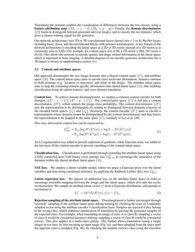
Latent regression loss. We impose an additional loss on the attribute latent space in order toencourage invertible mapping between the image and the latent space, which also aids the cyclicreconstruction. We sample an attribute latent vector zar from a Gaussian distribution, and attempt toreconstruct it:

Lza

1 = ‖Ea(G(Ec(x), zar ))− zar ‖1. (2)

Rejection sampling of the attribute latent space. Disentanglement is further encouraged through‘rejection’ sampling of the attribute latent space during training by checking the class of a randomlysampled vector using the attribute encoder’s classification layer. Samples are rejected if they belongto the wrong class, which stabilises optimisation of translation by passing the generator samples ofthe expected class. For example, when translating an image of class A to class B, sampling a vectorof class A would be considered incorrect, whereas sampling a vector of class B would be consideredcorrect. This also applies in a multi-class setting. This further allows translation (using a singleimage) in test time, by first encoding an input image (Fig. 4a), and then sampling from the space untilthe opposite class is sampled (Fig. 4b), by checking the random vector’s class using the classifier.

5

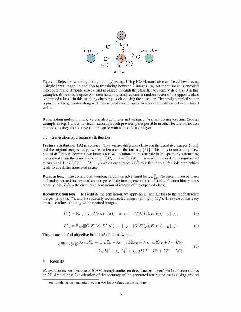
Figure 4: Rejection sampling during training/ testing. Using ICAM, translation can be achieved usinga single input image, in addition to translating between 2 images. (a) An input image is encodedinto content and attribute spaces, and is passed through the classifier to identify its class (0 in thisexample). (b) Attribute space A is then randomly sampled until a random vector of the opposite classis sampled (class 1 in this case), by checking its class using the classifier. The newly sampled vectoris passed to the generator along with the encoded content space to achieve translation between class 0and 1.

By sampling multiple times, we can also get mean and variance FA maps during test time (See anexample in Fig. 1 and 5), a visualisation approach previously not possible in other feature attributionmethods, as they do not have a latent space with a classification layer.

3.3 Generation and feature attribution

Feature attribution (FA) map loss. To visualise differences between the translated images {v, µ}and the original images {x, y}, we use a feature attribution map {M}. This aims to retain only class-related differences between two images (or two locations in the attribute latent space) by subtractingthe content from the translated output ({Mx = v − x}, {My = µ− y}). Generation is regularisedthrough an L1 loss (LM

1 = ‖M( )‖1,) which encourages {M} to reflect a small feasible map, whichleads to a realistic translated image.

Domain loss. The domain loss combines a domain adversarial loss, LDadv , (to discriminate between

real and generated images, and encourage realistic image generation) and a classification binary crossentropy loss, LD

BCE (to encourage generation of images of the expected class).

Reconstruction loss. To facilitate the generation, we apply an L1 and L2 loss to the reconstructedimages {x, y} (Lrec

1 ), and the cyclically reconstructed images {xcc, ycc} (Lcc1 ). The cycle consistency

term also allows training with unpaired images.

Lrec1,2 = Ex,y[‖G(Ec(x), Ea(x))− x‖1,2 + ‖G(Ec(y), Ea(y))− y‖1,2], (3)

Lcc1,2 = Ex,y[‖G(Ec(v), Ea(µ))− x‖1,2 + ‖G(Ec(µ), Ea(v))− y‖1,2]. (4)

This means the full objective function1 of our network is:

minG,Ec,Ea

maxD,Dc

λDcLDc

adv + λDLDadv + λDBCE

LDBCE + λBCEL

Ea

BCE + λKLLza

KL

+λMLM1 + λzaLza

1 + λrec(Lrec1 + Lcc

1 + Lrec2 + Lcc

2 ).(5)

4 Results

We evaluate the performance of ICAM through studies on three datasets to perform 1) ablation studieson 2D simulations; 2) evaluation of the accuracy of the generated attribution maps (using ground

1see supplementary materials section A.6 for λ values during training.

6

truth disease conversion maps derived from the ADNI dataset); 3) exploration of the flexibility of theapproach for investigating phenotypic variation (using healthy ageing data from UK Biobank).

4.1 Comparison methods and metrics

We compared our proposed approach against a range of baselines in our experiments. For a faircomparison, we use the same training, validation and testing datasets. In particular, we comparedagainst Grad-CAM, guided Grad-CAM [40], guided backprop [42], Integrated gradients [43],Occlusion [47], VA-GAN [5], and DRIT++ [28]. These methods were applied to both a simple3D ResNet (Table 3), and to the attribute encoder (Ea) of ICAM (Table 4). We compare against 2variations of the DRIT++ network, the original, DRITz8 , and with increased attribute latent spacesize (DRITz80 , size of 80 rather than 8), which is the same as ICAM. We also compared againstdifferent variations of our network, ICAM, including: ICAMDRIT , uses ICAM architecture, butall the same losses as in DRIT; ICAMBCE , which adds the classification BCE loss to the attributelatent space and rejection sampling during training; ICAMFA, which adds the FA map loss; andfinally ICAM , adding the l2 loss and thus containing all described losses in this paper. For furtherdetails on comparison methods, refer to supplementary section A.5.

Networks are compared using accuracy score for classification, and normalised cross correlation(NCC) between the absolute values of the attribution maps and the ground truth masks (e.g. the lesionmasks in the HCP lesion simulations, or the disease effect maps in ADNI). The positive NCC (+)compares the lesion mask to the attribution map when translating between class 0 (e.g. no lesions,or MCI) to 1 (e.g. lesions, or AD), and vice versa for the negative NCC (-). Values reported are themean and standard deviation across the test subjects.

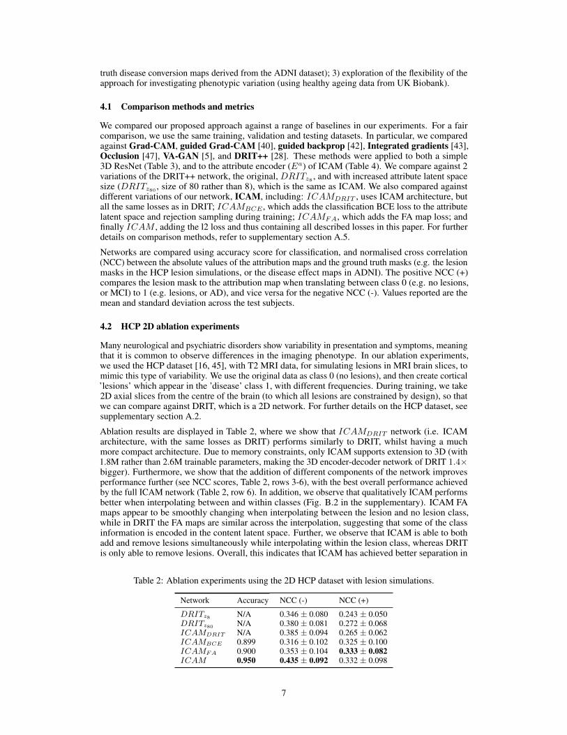
4.2 HCP 2D ablation experiments

Many neurological and psychiatric disorders show variability in presentation and symptoms, meaningthat it is common to observe differences in the imaging phenotype. In our ablation experiments,we used the HCP dataset [16, 45], with T2 MRI data, for simulating lesions in MRI brain slices, tomimic this type of variability. We use the original data as class 0 (no lesions), and then create cortical’lesions’ which appear in the ’disease’ class 1, with different frequencies. During training, we take2D axial slices from the centre of the brain (to which all lesions are constrained by design), so thatwe can compare against DRIT, which is a 2D network. For further details on the HCP dataset, seesupplementary section A.2.

Ablation results are displayed in Table 2, where we show that ICAMDRIT network (i.e. ICAMarchitecture, with the same losses as DRIT) performs similarly to DRIT, whilst having a muchmore compact architecture. Due to memory constraints, only ICAM supports extension to 3D (with1.8M rather than 2.6M trainable parameters, making the 3D encoder-decoder network of DRIT 1.4×bigger). Furthermore, we show that the addition of different components of the network improvesperformance further (see NCC scores, Table 2, rows 3-6), with the best overall performance achievedby the full ICAM network (Table 2, row 6). In addition, we observe that qualitatively ICAM performsbetter when interpolating between and within classes (Fig. B.2 in the supplementary). ICAM FAmaps appear to be smoothly changing when interpolating between the lesion and no lesion class,while in DRIT the FA maps are similar across the interpolation, suggesting that some of the classinformation is encoded in the content latent space. Further, we observe that ICAM is able to bothadd and remove lesions simultaneously while interpolating within the lesion class, whereas DRITis only able to remove lesions. Overall, this indicates that ICAM has achieved better separation in

Table 2: Ablation experiments using the 2D HCP dataset with lesion simulations.

Network Accuracy NCC (-) NCC (+)

DRITz8 N/A 0.346 ± 0.080 0.243 ± 0.050DRITz80 N/A 0.380 ± 0.081 0.272 ± 0.068ICAMDRIT N/A 0.385 ± 0.094 0.265 ± 0.062ICAMBCE 0.899 0.316 ± 0.102 0.325 ± 0.100ICAMFA 0.900 0.353 ± 0.104 0.333 ± 0.082ICAM 0.950 0.435 ± 0.092 0.332 ± 0.098

7

Table 3: ADNI experiments.

Network NCC (-) NCC (+)

Guided Grad-CAM [40] 0.244± 0.047 0.339± 0.068Grad-CAM [40] 0.321± 0.059 0.461± 0.086Occlusion [47] 0.360± 0.037 0.354± 0.057Integrated gradients [43] 0.378± 0.064 0.404± 0.059Guided backprop [42] 0.541± 0.054 0.532± 0.052VA-GAN [5] 0.653± 0.142 N/AICAM 0.683 ± 0.097 0.652 ± 0.083

the attribute latent space, and is further supported by the tSNE plots within class 1 (Fig. B.1 in thesupplementary).

4.3 ADNI experiments: Ground-truth evaluation of feature attribution maps

We use the longitudinal ADNI dataset [23], with T1 MRI data, as in Baumgartner et al. [5], to evaluatefeature attribution maps generated by ICAM and other baseline methods. DRIT [28] was not used asthe network design cannot scale to 3D due to memory constraints. ADNI contains paired examplesfor which images that are acquired before and after conversion to an AD state; where the intermediatestate between healthy cognition and AD is known as MCI. We used these subjects in our validationand test sets, to calculate the ground truth disease map (i.e. AD-specific brain atrophy patterns) foreach subject, which we then compared against the FA maps of each method to compute the NCCscore. See supplementary materials section A.3 for further details on the dataset.

We found that ICAM outperforms VA-GAN when comparing the NCC metric (Table 3), and that theyboth perform better than occlusion, integrated gradients, Grad-CAM, guided Grad-CAM and guidedbackprop. The FA maps generated by the VA-GAN in our comparisons differ to the original resultsof VA-GAN [5], and these differences might be accounted by a more strict data selection process(we picked images acquired with 3T only, and did not combine with 1.5T acquired images as inBaumgartner et al. [5]), which resulted in a smaller training size (5778 vs 931 subjects for training inVA-GAN and this work, respectively), and small differences in the pre-processing. In our experiments,we observe that ICAM is able to detect most of the real disease effects in ventricles, cortex, andhippocampus, but that VA-GAN only detects some of these differences (Fig. 1, and Fig. B.3 in thesupplementary). Both ICAM and VA-GAN generate higher resolution, and more interpretable FAmaps in comparison to occlusion, integrated gradients, Grad-CAM, guided Grad-CAM and guidedbackprop, suggesting that using generative models, instead of a simple classification CNN, might bea better approach for detecting more discriminative features, and phenotypic variability.

Finally, we tested whether ICAM FA generation performs better than FA methods (occlusion,integrated gradients and guided backprop) applied to ICAM’s attribute network Ea. We found that asexpected ICAM’s FA generation achieves better performance (using the NCC metric) than the FAmethods (Table 4).

4.4 Biobank experiments

We used T1 MRI data from the UK Biobank [1, 32], a collection of brain imaging data of mostlyhealthy subjects between the ages of 44-80 years old, to study phenotypic variation that occurs duringageing. To use this dataset for classification, we split the data into 2 classes, of young (class 0,

Table 4: ADNI experiments with ICAM Ea.

Network NCC (-) NCC (+)

ICAM-Ea Occlusion 0.235 ± 0.067 0.310 ± 0.047ICAM-Ea Integrated gradients 0.269 ± 0.054 0.289 ± 0.046ICAM-Ea Guided backprop 0.295 ± 0.056 0.301 ± 0.044ICAM 0.683 ± 0.097 0.652 ± 0.083

8

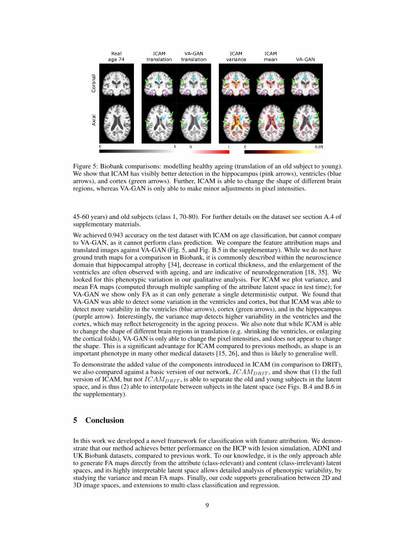
Figure 5: Biobank comparisons: modelling healthy ageing (translation of an old subject to young).We show that ICAM has visibly better detection in the hippocampus (pink arrows), ventricles (bluearrows), and cortex (green arrows). Further, ICAM is able to change the shape of different brainregions, whereas VA-GAN is only able to make minor adjustments in pixel intensities.

45-60 years) and old subjects (class 1, 70-80). For further details on the dataset see section A.4 ofsupplementary materials.

We achieved 0.943 accuracy on the test dataset with ICAM on age classification, but cannot compareto VA-GAN, as it cannot perform class prediction. We compare the feature attribution maps andtranslated images against VA-GAN (Fig. 5, and Fig. B.5 in the supplementary). While we do not haveground truth maps for a comparison in Biobank, it is commonly described within the neurosciencedomain that hippocampal atrophy [34], decrease in cortical thickness, and the enlargement of theventricles are often observed with ageing, and are indicative of neurodegeneration [18, 35]. Welooked for this phenotypic variation in our qualitative analysis. For ICAM we plot variance, andmean FA maps (computed through multiple sampling of the attribute latent space in test time); forVA-GAN we show only FA as it can only generate a single deterministic output. We found thatVA-GAN was able to detect some variation in the ventricles and cortex, but that ICAM was able todetect more variability in the ventricles (blue arrows), cortex (green arrows), and in the hippocampus(purple arrow). Interestingly, the variance map detects higher variability in the ventricles and thecortex, which may reflect heterogeneity in the ageing process. We also note that while ICAM is ableto change the shape of different brain regions in translation (e.g. shrinking the ventricles, or enlargingthe cortical folds), VA-GAN is only able to change the pixel intensities, and does not appear to changethe shape. This is a significant advantage for ICAM compared to previous methods, as shape is animportant phenotype in many other medical datasets [15, 26], and thus is likely to generalise well.

To demonstrate the added value of the components introduced in ICAM (in comparison to DRIT),we also compared against a basic version of our network, ICAMDRIT , and show that (1) the fullversion of ICAM, but not ICAMDRIT , is able to separate the old and young subjects in the latentspace, and is thus (2) able to interpolate between subjects in the latent space (see Figs. B.4 and B.6 inthe supplementary).

5 Conclusion

In this work we developed a novel framework for classification with feature attribution. We demon-strate that our method achieves better performance on the HCP with lesion simulation, ADNI andUK Biobank datasets, compared to previous work. To our knowledge, it is the only approach ableto generate FA maps directly from the attribute (class-relevant) and content (class-irrelevant) latentspaces, and its highly interpretable latent space allows detailed analysis of phenotypic variability, bystudying the variance and mean FA maps. Finally, our code supports generalisation between 2D and3D image spaces, and extensions to multi-class classification and regression.

9

Broader Impact

There is growing evidence that deep learning tools have the potential to improve the speed of reviewof medical images and that their sensitivity to complex high-dimensional textures can (in some cases)improve their efficacy relative to radiographers [19]. A recent study by Google DeepMind [31]suggested that deep learning systems could perform the role of a second-reader of breast cancerscreenings to improve the precision of diagnosis relative to a single-expert (which is standard clinicalpractice within the US).

For brain disorders the opportunities and challenges for AI are more significant since the featuresof the disease are commonly subtle, presentations highly variable (creating greater challenges forphysicians), and the datasets are much smaller in size in comparison to natural image tasks. Theadditional pitfalls that are common in deep learning algorithms [46], including the so called ‘blackbox’ problem where it is unknown why a certain prediction is made, lead to further uncertainly andmistrust for clinicians when making decisions based on the results of these models.

We developed a novel framework to address this problem by deriving a disease map, directly from aclass prediction space, which highlights all class relevant features in an image. Our objective is todemonstrate on a theoretical level, that the development of more medically interpretable models isfeasible, rather than developing a diagnostic tool to be used in the clinic. However, in principle, thesetypes of maps may be used by physicians as an additional source of data in addition to mental exams,physiological tests and their own judgement to support diagnosis of complex conditions such asAlzheimer’s, autism, and schizophrenia. This may have significant societal impact as early diagnosiscan improve the effectiveness of interventional treatment. Further, our model, ICAM, presents aspecific advantage as it provides a ‘probability’ of belonging to a class along with a visualisation,supporting better understanding of the phenotypic variation of these diseases, which may improvemechanistic or prognostic modelling of these diseases.

There remain ethical challenges as errors in prediction could influence clinicians towards wrongdiagnoses and incorrect treatment which could have very serious consequences. Further studies haveshown clear racial differences in brain structure [41, 44] which if not sampled correctly could lead tobias in the model and greater uncertainty for ethnic minorities [39]. These challenges would need tobe addressed before any consideration of clinical translation. Clearly, the uncertainties in the modelshould be transparently conveyed to any end user, and in this respect the advantages of ICAM relativeto its predecessors are plain to see.

Acknowledgments and Disclosure of Funding

The work of E.C.R. and C.B. was supported by the Academy of Medical Sciences/the British HeartFoundation/the Government Department of Business, Energy and Industrial Strategy/the WellcomeTrust Springboard Award [SBF003/1116] and E.C.R., C.B. and S.M.S. are supported by WellcomeCollaborative Award [215573/Z/19/Z]. PD.T. was supported by the EPSRC Research Council, partof the EPSRC DTP [EP/R513064/1]. M. DS. would like to acknowledge funding from the EPSRCCentre for Doctoral Training in Smart Medical Imaging [EP/S022104/1].

The ADNI data used in this work was funded by the Alzheimer’s Disease Neuroimaging Initiative(ADNI) (National Institutes of Health Grant U01 AG024904) and DOD ADNI (Department ofDefense award number W81XWH-12-2-0012). The UK Biobank data was accessed under Appli-cation Number 8107. The HCP data was provided by the Human Connectome Project, WU-MinnConsortium (Principal Investigators: David Van Essen and Kamil Ugurbil; 1U54MH091657) fundedby the 16 NIH Institutes and Centers that support the NIH Blueprint for Neuroscience Research; andby the McDonnell Center for Systems Neuroscience at Washington University.

We would also like to thank Kai Arulkumaran and Ankur Handa for valuable comments and sugges-tions during manuscript writing.

The Authors declare that there is no conflict of interest.

10

References[1] F. Alfaro-Almagro, M. Jenkinson, N. K. Bangerter, J. L. Andersson, L. Griffanti, G. Douaud, S. N.

Sotiropoulos, S. Jbabdi, M. Hernandez-Fernandez, E. Vallee, et al. Image processing and quality controlfor the first 10,000 brain imaging datasets from uk biobank. Neuroimage, 166:400–424, 2018.

[2] B. B. Avants, P. Yushkevich, J. Pluta, D. Minkoff, M. Korczykowski, J. Detre, and J. C. Gee. The optimaltemplate effect in hippocampus studies of diseased populations. Neuroimage, 49(3):2457–2466, 2010.

[3] S. Bach, A. Binder, G. Montavon, F. Klauschen, K.-R. Müller, and W. Samek. On pixel-wise explanationsfor non-linear classifier decisions by layer-wise relevance propagation. PloS one, 10(7), 2015.

[4] C. Bass, T. Dai, B. Billot, K. Arulkumaran, A. Creswell, C. Clopath, V. De Paola, and A. A. Bharath.Image synthesis with a convolutional capsule generative adversarial network. Medical Imaging with DeepLearning, 2019.

[5] C. F. Baumgartner, L. M. Koch, K. Can Tezcan, J. Xi Ang, and E. Konukoglu. Visual feature attribution us-ing wasserstein gans. In Proceedings of the IEEE Conference on Computer Vision and Pattern Recognition,pages 8309–8319, 2018.

[6] C. Baur, B. Wiestler, S. Albarqouni, and N. Navab. Deep autoencoding models for unsupervised anomalysegmentation in brain mr images. In International MICCAI Brainlesion Workshop, pages 161–169.Springer, 2018.

[7] J. D. Bijsterbosch, M. W. Woolrich, M. F. Glasser, E. C. Robinson, C. F. Beckmann, D. C. Van Essen, S. J.Harrison, and S. M. Smith. The relationship between spatial configuration and functional connectivity ofbrain regions. Elife, 7:e32992, 2018.

[8] H. Chen, Q. Dou, L. Yu, J. Qin, and P.-A. Heng. Voxresnet: Deep voxelwise residual networks for brainsegmentation from 3d mr images. NeuroImage, 170:446–455, 2018.

[9] P. Costa, A. Galdran, M. I. Meyer, M. Niemeijer, M. Abràmoff, A. M. Mendonça, and A. Campilho.End-to-end adversarial retinal image synthesis. IEEE transactions on medical imaging, 37(3):781–791,2017.

[10] H. Cullen, M. L. Krishnan, S. Selzam, G. Ball, A. Visconti, A. Saxena, S. J. Counsell, J. Hajnal, G. Breen,R. Plomin, et al. Polygenic risk for neuropsychiatric disease and vulnerability to abnormal deep greymatter development. Scientific reports, 9(1):1–8, 2019.

[11] A. Dalca, M. Rakic, J. Guttag, and M. Sabuncu. Learning conditional deformable templates with convolu-tional networks. In Advances in neural information processing systems, pages 804–816, 2019.

[12] A. V. Dalca, G. Balakrishnan, J. Guttag, and M. R. Sabuncu. Unsupervised learning of probabilisticdiffeomorphic registration for images and surfaces. Medical image analysis, 57:226–236, 2019.

[13] A. de Brebisson and G. Montana. Deep neural networks for anatomical brain segmentation. In Proceedingsof the IEEE conference on computer vision and pattern recognition workshops, pages 20–28, 2015.

[14] A. C. Evans, A. L. Janke, D. L. Collins, and S. Baillet. Brain templates and atlases. Neuroimage, 62(2):911–922, 2012.

[15] K. E. Garcia, E. C. Robinson, D. Alexopoulos, D. L. Dierker, M. F. Glasser, T. S. Coalson, C. M. Ortinau,D. Rueckert, L. A. Taber, D. C. Van Essen, et al. Dynamic patterns of cortical expansion during folding ofthe preterm human brain. Proceedings of the National Academy of Sciences, 115(12):3156–3161, 2018.

[16] M. F. Glasser, T. S. Coalson, E. C. Robinson, C. D. Hacker, J. Harwell, E. Yacoub, K. Ugurbil, J. Andersson,C. F. Beckmann, M. Jenkinson, et al. A multi-modal parcellation of human cerebral cortex. Nature, 536(7615):171–178, 2016.

[17] I. Goodfellow, Y. Bengio, and A. Courville. Deep learning. MIT press, 2016.

[18] H. Guo, W. Siu, R. C. D’Arcy, S. E. Black, L. A. Grajauskas, S. Singh, Y. Zhang, K. Rockwood, andX. Song. Mri assessment of whole-brain structural changes in aging. Clinical interventions in aging, 12:1251, 2017.

[19] A. Hosny, C. Parmar, J. Quackenbush, L. H. Schwartz, and H. J. Aerts. Artificial intelligence in radiology.Nature Reviews Cancer, 18(8):500–510, 2018.

[20] X. Huang, M.-Y. Liu, S. Belongie, and J. Kautz. Multimodal unsupervised image-to-image translation. InProceedings of the European Conference on Computer Vision (ECCV), pages 172–189, 2018.

[21] K. Iqbal, M. Flory, S. Khatoon, H. Soininen, T. Pirttila, M. Lehtovirta, I. Alafuzoff, K. Blennow, N. An-dreasen, E. Vanmechelen, et al. Subgroups of alzheimer’s disease based on cerebrospinal fluid molecularmarkers. Annals of Neurology: Official Journal of the American Neurological Association and the ChildNeurology Society, 58(5):748–757, 2005.

[22] P. Isola, J.-Y. Zhu, T. Zhou, and A. A. Efros. Image-to-image translation with conditional adversarialnetworks. In Proceedings of the IEEE conference on computer vision and pattern recognition, pages1125–1134, 2017.

11

[23] C. R. Jack Jr, M. A. Bernstein, N. C. Fox, P. Thompson, G. Alexander, D. Harvey, B. Borowski, P. J.Britson, J. L. Whitwell, C. Ward, et al. The alzheimer’s disease neuroimaging initiative (adni): Mrimethods. Journal of Magnetic Resonance Imaging: An Official Journal of the International Society forMagnetic Resonance in Medicine, 27(4):685–691, 2008.

[24] A. H. Jha, S. Anand, M. Singh, and V. Veeravasarapu. Disentangling factors of variation with cycle-consistent variational auto-encoders. In European Conference on Computer Vision, pages 829–845.Springer, 2018.

[25] K. Kamnitsas, W. Bai, E. Ferrante, S. McDonagh, M. Sinclair, N. Pawlowski, M. Rajchl, M. Lee, B. Kainz,D. Rueckert, et al. Ensembles of multiple models and architectures for robust brain tumour segmentation.In International MICCAI Brainlesion Workshop, pages 450–462. Springer, 2017.

[26] O. Kapellou, S. J. Counsell, N. Kennea, L. Dyet, N. Saeed, J. Stark, E. Maalouf, P. Duggan, M. Ajayi-Obe,J. Hajnal, et al. Abnormal cortical development after premature birth shown by altered allometric scalingof brain growth. PLoS medicine, 3(8), 2006.

[27] R. Kong, J. Li, C. Orban, M. R. Sabuncu, H. Liu, A. Schaefer, N. Sun, X.-N. Zuo, A. J. Holmes, S. B.Eickhoff, et al. Spatial topography of individual-specific cortical networks predicts human cognition,personality, and emotion. Cerebral cortex, 29(6):2533–2551, 2019.

[28] H.-Y. Lee, H.-Y. Tseng, Q. Mao, J.-B. Huang, Y.-D. Lu, M. Singh, and M.-H. Yang. Drit++: Diverseimage-to-image translation via disentangled representations. arXiv preprint arXiv:1905.01270, 2019.

[29] M.-Y. Liu, T. Breuel, and J. Kautz. Unsupervised image-to-image translation networks. In Advances inneural information processing systems, pages 700–708, 2017.

[30] S. M. Lundberg and S.-I. Lee. A unified approach to interpreting model predictions. In Advances in neuralinformation processing systems, pages 4765–4774, 2017.

[31] S. M. McKinney, M. Sieniek, V. Godbole, J. Godwin, N. Antropova, H. Ashrafian, T. Back, M. Chesus,G. C. Corrado, A. Darzi, et al. International evaluation of an ai system for breast cancer screening. Nature,577(7788):89–94, 2020.

[32] K. L. Miller, F. Alfaro-Almagro, N. K. Bangerter, D. L. Thomas, E. Yacoub, J. Xu, A. J. Bartsch, S. Jbabdi,S. N. Sotiropoulos, J. L. Andersson, et al. Multimodal population brain imaging in the uk biobankprospective epidemiological study. Nature neuroscience, 19(11):1523, 2016.

[33] G. Montavon, S. Bach, A. Binder, W. Samek, and K.-R. Muller. Deep taylor decomposition of neuralnetworks. In International Conference on Machine Learning workshop on Visualization for Deep Learning,2016.

[34] A. O’Shea, R. Cohen, E. C. Porges, N. R. Nissim, and A. J. Woods. Cognitive aging and the hippocampusin older adults. Frontiers in aging neuroscience, 8:298, 2016.

[35] J. Pacheco, J. O. Goh, M. A. Kraut, L. Ferrucci, and S. M. Resnick. Greater cortical thinning in normalolder adults predicts later cognitive impairment. Neurobiology of aging, 36(2):903–908, 2015.

[36] M. Rajchl, N. Pawlowski, D. Rueckert, P. M. Matthews, and B. Glocker. Neuronet: fast and robustreproduction of multiple brain image segmentation pipelines. arXiv preprint arXiv:1806.04224, 2018.

[37] E. C. Robinson, K. Garcia, M. F. Glasser, Z. Chen, T. S. Coalson, A. Makropoulos, J. Bozek, R. Wright,A. Schuh, M. Webster, et al. Multimodal surface matching with higher-order smoothness constraints.NeuroImage, 167:453–465, 2018.

[38] C. A. Ross, R. L. Margolis, S. A. Reading, M. Pletnikov, and J. T. Coyle. Neurobiology of schizophrenia.Neuron, 52(1):139–153, 2006.

[39] N. M. Safdar, J. D. Banja, and C. C. Meltzer. Ethical considerations in artificial intelligence. EuropeanJournal of Radiology, 122:108768, 2020.

[40] R. R. Selvaraju, M. Cogswell, A. Das, R. Vedantam, D. Parikh, and D. Batra. Grad-cam: Visual explanationsfrom deep networks via gradient-based localization. In Proceedings of the IEEE international conferenceon computer vision, pages 618–626, 2017.

[41] L. Shi, P. Liang, Y. Luo, K. Liu, V. C. Mok, W. C. Chu, D. Wang, and K. Li. Using large-scalestatistical chinese brain template (chinese2020) in popular neuroimage analysis toolkits. Frontiers inhuman neuroscience, 11:414, 2017.

[42] J. T. Springenberg, A. Dosovitskiy, T. Brox, and M. Riedmiller. Striving for simplicity: The all convolu-tional net. arXiv preprint arXiv:1412.6806, 2014.

[43] M. Sundararajan, A. Taly, and Q. Yan. Axiomatic attribution for deep networks. In Proceedings of the34th International Conference on Machine Learning-Volume 70, pages 3319–3328. JMLR. org, 2017.

[44] Y. Tang, L. Zhao, Y. Lou, Y. Shi, R. Fang, X. Lin, S. Liu, and A. Toga. Brain structure differences betweenc hinese and c aucasian cohorts: A comprehensive morphometry study. Human brain mapping, 39(5):2147–2155, 2018.

12

[45] D. C. Van Essen, K. Ugurbil, E. Auerbach, D. Barch, T. Behrens, R. Bucholz, A. Chang, L. Chen, M. Cor-betta, S. W. Curtiss, et al. The human connectome project: a data acquisition perspective. Neuroimage, 62(4):2222–2231, 2012.

[46] E. Vayena, A. Blasimme, and I. G. Cohen. Machine learning in medicine: addressing ethical challenges.PLoS medicine, 15(11), 2018.

[47] M. D. Zeiler and R. Fergus. Visualizing and understanding convolutional networks. In European conferenceon computer vision, pages 818–833. Springer, 2014.

[48] J.-Y. Zhu, T. Park, P. Isola, and A. A. Efros. Unpaired image-to-image translation using cycle-consistentadversarial networks. In Proceedings of the IEEE international conference on computer vision, pages2223–2232, 2017.

13