Internationale Kommission für die Hydrologie des ...
228
Internationale Kommission für die Hydrologie des Rheingebietes International Commission for the Hydrology of the Rhine Basin Assessment of Climate Change Impacts on Discharge in the Rhine River Basin: Results of the RheinBlick2050 Project Klaus Görgen, Centre de Recherche Public - Gabriel Lippmann, Luxembourg Jules Beersma, Koninklijk Nederlands Meteorologisch Instituut, The Netherlands Gerhard Brahmer, Hessisches Landesamt für Umwelt und Geologie, Germany Hendrik Buiteveld, Rijkswaterstaat, The Netherlands Maria Carambia, Bundesanstalt für Gewässerkunde, Germany Otto de Keizer, Deltares, The Netherlands Peter Krahe, Bundesanstalt für Gewässerkunde, Germany Enno Nilson, Bundesanstalt für Gewässerkunde, Germany Rita Lammersen, Rijkswaterstaat, The Netherlands Charles Perrin, Cemagref, France David Volken, Bundesamt für Umwelt BAFU, Switzerland Authors are in alphabetical order with the project coordinator and report editor first. See also the RheinBlick2050 Project Group page for further contributors and members. Report No. I-23 of the CHR © 2010, CHR ISBN 978-90-70980-35-1 Koninklijk Nederlands Meteorologisch Instituut Ministerie van Verkeer en Waterstaat Rijkswaterstaat Ministerie van Verkeer en Waterstaat
Transcript of Internationale Kommission für die Hydrologie des ...
Internationale Kommission für die Hydrologie des Rheingebietes
International Commission for the Hydrology of the Rhine Basin
Assessment of Climate Change Impacts on Discharge in the Rhine River Basin: Results of the RheinBlick2050 Project
Klaus Görgen, Centre de Recherche Public - Gabriel Lippmann, Luxembourg Jules Beersma, Koninklijk Nederlands Meteorologisch Instituut, The Netherlands Gerhard Brahmer, Hessisches Landesamt für Umwelt und Geologie, Germany Hendrik Buiteveld, Rijkswaterstaat, The Netherlands Maria Carambia, Bundesanstalt für Gewässerkunde, Germany Otto de Keizer, Deltares, The Netherlands Peter Krahe, Bundesanstalt für Gewässerkunde, Germany Enno Nilson, Bundesanstalt für Gewässerkunde, Germany Rita Lammersen, Rijkswaterstaat, The Netherlands Charles Perrin, Cemagref, France David Volken, Bundesamt für Umwelt BAFU, Switzerland Authors are in alphabetical order with the project coordinator and report editor first. See also the RheinBlick2050 Project Group page for further contributors and members.
Report No. I-23 of the CHR © 2010, CHR ISBN 978-90-70980-35-1
Koninklijk Nederlands Meteorologisch Instituut Ministerie van Verkeer en Waterstaat
Rijkswaterstaat Ministerie van Verkeer en Waterstaat
IV
Reading Guide
Dear Reader,
this project assesses selected aspects of the impacts of climate change on discharge in the Rhine River basin. It does not deal with adaptation or mitigation strategies. The study has been set up using a comprehensive modelling and analysis framework as well as state of the art data, models and methods. Nevertheless, there are specific restrictions and limitations, which are e.g. related to data availability, model assumptions, as well as limited resources and the specific experiment designs of the different projects contributing to the study.
The report has a scientific scope and represents state of the art scientific knowledge. The target groups of this report are scientists working in the field and representatives from technical government authorities. Despite this, the project is part of a science to policy process within the International Commission for the Protection of the Rhine (ICPR) Expert Group “Klima”, where results of RheinBlick2050 are used together with other sources of information to develop common climate change scenarios that might be used later in politically relevant climate adaptation strategies.
The limitations and constraints of the study have to be fully understood in order to properly comprehend results, conclusions and uncertainties. The report deals extensively with such issues, e.g. in Chapters 1 to 3. In order to avoid misinterpretations, we strongly recommend reading the report completely! Nevertheless, below we give an overview of the most relevant limitations and constraints. Remember that the text below is an excerpt; it only touches on the issues in a highly abbreviated form; it is intentionally redundant with other parts of the main text. An overview on the structure of the report is given at the end of Chapter 1.
In case of any question or doubt: Please do not hesitate to contact the International Commission for the Hydrology of the Rhine Basin (CHR) or the authors.
The RheinBlick2050 report authors, September 2010
Limitations and constraints
Projections not predictions This report, i.e. the RheinBlick2050 project, offers hydrological projections for the future climate that are based on the current understanding of the climate system and the hydrology of the Rhine basin. There are limitations and scientific unknowns that might affect the information provided. Therefore, this report and the RheinBlick2050 project only provide possible hydrological projections rather than absolute predictions or forecasts of the hydrology of the Rhine River for a potential future climate.
Target spatial scale This study has a spatial focus on the entire Rhine River basin. Results are provided for the main Rhine River gauges and gauging stations situated on the major subcatchments of the Rhine River basin (Main, Moselle). Data, modelling tools and analyses methodologies have been chosen and optimized according to this spatial scale.
V
Consistency For different parts of the report varying datasets and methods have proven to be suitable. As a consequence, in different chapters different model couplings have been used. Nevertheless, there are several model couplings that are used throughout the report (e.g. A1B_EH5r1_REMO_HBV).
Model and data validity All models represent a simplification of reality. Thus, they can not be expected to reproduce observed values exactly. In addition, observed data which are used to calibrate and validate models are not free from errors either.
In this study the model chain ends with hydrological models, which do not consider hydraulic effects to a full extend. For example the damping of the flood wave by overtopping of dikes and the backwater effect in the tributaries are not taken into account. In case of the extreme discharges one therefore has to keep in mind that the simulated discharges are likely too high and care has to be taken with the interpretation.
Sampling Although many data resources have been included in the report to account for the full range of knowledge about future developments, one has to be aware that the “real” range in possible futures is still unknown:
a) We have limited knowledge about the “true” complexity of climate and hydrological system dynamics.
b) There are generally limited computational and project resources and therefore not all possible couplings of emission scenarios with global and regional climate models and hydrological models can be done.
c) Not all models are taken into account since they are not suitable within the framework of this study.
Example: The EU-ENSEMBLES project is the primary data source for the regional climate change projections. Although an extensive model matrix with many global and regional climate model combinations was developed, there is a clear domination of ECHAM5 and HadCM3 global models; hence the regional climate model results are very much influenced by the characteristics of these two global models. In addition most climate model projections are based on the A1B emission scenario while other emission scenarios may be equally likely.
“State of the art knowledge” This report is “state of the art” in the year 2010. As climate change research is a fast evolving field of science, the “state of the art” may change in due time. As a consequence, the results presented here have to be re-evaluated regularly.
Example: The global climate models conducted since 2000 used here result from the Coupled Model Intercomparison Project 3 (CMIP3), which is the basis of the 4th Intergovernmental Panel on Climate Change (IPCC) assessment report. Currently, new runs are underway in CMIP5 which include many improvements and which will be the basis of the 5th IPCC assessment report. These runs will most likely produce other results than the ones used here. Likewise new generations of hydrological models are going to yield new and differing results.

VI
CHR / RheinBlick2050 Project Group
Members and contributing report authors
Dr. Klaus Görgen (project coordinator, report editor) Public Research Centre – Gabriel Lippmann (CRP-GL) Department of Environment and Agro-Biotechnologies 41, rue du Brill 4422 Belvaux Luxembourg phone: +352.470261-461 e-mail: [email protected] http://www.lippmann.lu
Dr. Jules Beersma Royal Netherlands Meteorological Institute (KNMI) Climate Services P.O. Box 201 3730 AE De Bilt The Netherlands phone: +31.30-2206-475 e-mail: [email protected] http://www.knmi.nl
Ir. Hendrik Buiteveld Rijkswaterstaat Centre for Water Management (RWS) Department of International Coordination Postbus 17 8200 AA Lelystad The Netherlands phone: +31.65-3649-418 e-mail: [email protected] http://www.rijkswaterstaat.nl
Dr. Gerhard Brahmer Hessisches Landesamt für Umwelt und Geologie (HLUG) Dezernat Hydrologie, Hochwasserschutz Rheingaustrasse 186 65203 Wiesbaden Germany phone: phone: +49.611-6939-737 e-mail: [email protected] http://www.hlug.de
Dipl. Ing. Maria Carambia Federal Institute of Hydrology (BfG) Department Water Balance, Forecasting and Predictions Am Mainzer Tor 1 56068 Koblenz Germany phone: +49.261-1306-5491 e-mail: [email protected] http://www.bafg.de
Ir. Otto de Keizer Deltares Unit Inland Water Systems Rotterdamseweg 185 2629 HD Delft The Netherlands phone: +31.88-335-7657 e-mail: [email protected] http://www.deltares.nl
Dipl. Met. Peter Krahe Federal Institute of Hydrology (BfG) Department Water Balance, Forecasting and Predictions Am Mainzer Tor 1 56068 Koblenz Germany phone: +49.261-1306-5234 e-mail: [email protected] http://www.bafg.de
Dr. Rita Lammersen Rijkswaterstaat Centre for Water Management (RWS) Department of Flood Risk Management Postbus 17 8200 AA Lelystad The Netherlands phone: +31.65-192-3811 e-mail: [email protected] http://www.rijkswaterstaat.nl
Dr. Enno Nilson Federal Institute of Hydrology (BfG) Department Water Balance, Forecasting and Predictions Am Mainzer Tor 1
Dr. Charles Perrin Cemagref Hydrosystems and Bioprocesses Research Unit (HBAN) Parc de Tourvoie
VII
56068 Koblenz Germany phone: +49.261-1306-5325 e-mail: [email protected] http://www.bafg.de
BP 44 92163 Antony Cedex France phone: +33.1-4096-6086 e-mail: [email protected] http://www.cemagref.fr
Dr. David Volken Federal Office for the Environment (FOEN) Hydrology Division Papiermühlestrasse 172 3063 Ittigen Switzerland phone: +41.31-324-7927 e-mail: [email protected] http://www.bafu.admin.ch
Information in this table is valid as of September 2010.
Further members and project contributors The following people belonged for either the complete duration or at least for some time to the RheinBlick2050 project group and also contributed substantially to the project and the final report either by providing data and software tools, by their active participation in the various project meetings or vivid discussions and thorough revisions on parts of the report.
Dipl. Natw. ETH Thomas Bosshard, Eidgenössische Technische Hochschule Zürich, Zürich, Switzerland
Dr. Houda Boudhraa, ex Cemagref, Antony, France
Dr. Jaap Kwadijk, Deltares, Delft, The Netherlands
Dr. Laurent Pfister, Centre de Recherche Public – Gabriel Lippmann, Belvaux, Luxembourg
Dr. Bruno Schädler, ex Bundesamt für Umwelt BAFU, Bern, Switzerland
Ir. Frederiek Sperna-Weiland, Deltares, Delft, The Netherlands
Ing. Eric Sprokkereef, Rijkswaterstaat, Lelystad, The Netherlands
Dr. Pierre-Francois Staub, ex Cemagref, Antony, France
Acknowledgements
Regional climate model were kindly provided primarily within the framework of the EU FP6 Integrated Project ENSEMBLES (Contract number 505539). Additional model runs were provided by the Max Planck Institute of Meteorology in Hamburg on behalf of the German Federal Environment Agency (REMO-UBA) and the German Federal Institute of Hydrology (REMO-BFG), within the frame work of the research initiative “klimazwei” (CCLM, funded by the German Ministry of Research), by Climate & Environment Consulting Potsdam GmbH (CEC) on behalf of the German Federal Environment Agency (WETTREG-UBA) and by the Potsdam Institute for Climate Impact Research (STAR-PIK). The German Federal States and Rijkswaterstaat kindly provided statistical values for MHQ, HQ10, HQ100 and HQ1000 for the gauging stations used in the RheinBlick2050 project (these statistics are further denoted as “PROV_STAT”). We would like to thank all involved research groups!
VIII
We would further more like to thank all meteorological and water management institutions that have provided meteorological and hydrological observations.
RheinBlick2050 is designed as a “meta”-project that, based on some basic funding by the CHR for coordination, incorporated and linked different (independent) ongoing efforts and projects, combining datasets, methodologies and results. Therefore the financial contributions of various organisations to make the participation of some of their members possible are gratefully acknowledged:
- In addition to the CHR, the CRP-Gabriel Lippmann provided funding for the project coordination. CRP-GL also fully funded the Luxembourgish scientific contributions as well as computational support to the project.
- KNMI contributions were funded by the Dutch Ministry for Transport and Water Management and partly by the EU FP6 ENSEMBLES project.
- Rijkswaterstaat contribuations were financed by the Dutch Ministry for Transport and Water Management.
- The contributions of the German Federal Institute of Hydrology (BfG) were provided within the framework of the KLIWAS research programme (project KLIWAS 4.01 Water Balance, Water Level, Transport Capacity) and financed by the German Federal Ministry of Transport, Building and Urban Development.
- The Deltares contributions were financed by the Rijkswaterstaat Centre for Water Management, as part of a subsidy for applied research by Deltares.
- Cemagref’s contribution was possible through the financial support from the Agence de l'Eau Rhin-Meuse, Metz, France and Cemagref's General Direction.
- The effects of climate change on water resources and water courses was investigated in the framework of the project CCHydro, launched by the Swiss Federal Office for the Environment (FOEN) in 2007. Some climate and discharge scenarios were kindly provided within the project CCHydro by the Institute of Atmospheric and Climate Science at ETH Zurich.
We would also like to thank helpful colleagues at the various institutions involved: Saskia Buchholz (CRP-GL), Adri Buishand (KNMI), Martin Ebel (Deltares), Jürgen Junk (CRP-GL), Hanneke van der Klis (Deltares). They helped reviewing and thereby improving the complete report or parts of it.
IX
Foreword
„Eigentlich weiss man nur, wenn man wenig weiss. Mit dem Wissen wächst der Zweifel; hier kann RheinBlick2050 helfen.“
Frei nach Goethe
For some time the International Commission for the Hydrology of the Rhine Basin (CHR) is engaged with the investigation of the impacts of climate change on discharge of the Rhine River and its major tributaries. First calculations and insights were published in 1997 in the CHR publication I-16. Those results let to the recommendation (Nijmegener declaration) to the water authorities in the riparian states to follow a “policy of no regret” with regard to the changing discharge behaviour of the Rhine River.
Since 1997 climate change research has made big progress. Thus the question arose whether this advancement in knowledge would lead to improved projections of future discharge changes of the Rhine River. In order to answer this question the CHR drafted the project RheinBlick2050. It has the objective to investigate the effects of climate change on Rhine River discharge based on the latest state of the art. A working group with experts from several research institutions and technical water agencies conducted the analyses and the results are now available. They are summarised in the present report.
The CHR as a scientific institution provides its findings as a basis for decision making to responsible authorities of integral water management. As an example, results of the report are going to be incorporated into work of the International Commission for the Protection of the Rhine (ICPR).
The CHR would like to thank the international working group, led by Dr. K. Görgen, for the excellent realisation of the investigations and the report compilation. Thanks also to the CHR secretariat, the scientific secretary of the CHR, E. Sprokkereef, and the member states coordinators.
Prof. Dr. Manfred Spreafico
President of the International Commission for the Hydrology of the Rhine
X
General Information on the International Commission for the Hydrology of the Rhine Basin (CHR)
The CHR is an organisation in which scientific institutions of the riparian countries of the Rhine River develop joint fundamental hydrological information for a sustainable development in the Rhine River region.
Mission and tasks of the CHR Extension of the knowledge on the hydrology of the Rhine River basin through:
• Joint research
• Exchange of data, methods and information
• Development of standardized procedures
Contribution to the solution of transboundary problems through the formulation, management and provision of:
• Information systems (e.g. CHR Rhine GIS)
• Models, e.g. water-balance models and the Rhine Alarm Model
Member countries Switzerland, Austria, Germany, France, Luxembourg and The Netherlands
Participating institutions
Bundesministerium für Land- und Forstwirtschaft, Umwelt und Wasserwirtschaft Hydrografisches Zentralbüro Vienna, Austria http://www.lebensministerium.at
Amt der Vorarlberger Landesregierung Abteilung Wasserwirtschaft Bregenz, Austria http://www.vorarlberg.at
Federal Office for the Environment Bern, Switzerland http://www.bafu.admin.ch
Federal Institute of Hydrology Koblenz, Germany http://www.bafg.de

XI
German IHP/HWRP National Committee Koblenz, Germany http://ihp.bafg.de
Hessisches Landesamt für Umwelt und Geologie Wiesbaden, Germany http://www.hlug.de
Administration de la Gestion de l'Eau Luxembourg http://www.etat.lu/eau
Cemagref Antony, France http://www.cemagref.fr
Rijkswaterstaat Centre for Water Management Lelystad, The Netherlands http://www.rijkswaterstaat.nl
Deltares Delft, The Netherlands http://www.deltares.nl
Relationship to UNESCO and WMO The CHR was founded in 1970 on the occasion of a recommendation by the United Nations Educational, Scientific and Cultural Organization (UNESCO) to promote a closer collaboration in international river basins. Since 1975 work has been extended within the framework of the International Hydrological Programme (IHP) of the UNESCO and the Hydrological Water Resources Programme (HWRP) of the World Meteorological Organisation (WMO).
For more information on the CHR, see the website: http://www.chr-khr.org

XIII
Table of Contents1
Reading Guide .................................................................................................................... IV CHR / RheinBlick2050 Project Group ............................................................................... VI Acknowledgements ........................................................................................................... VII Foreword ............................................................................................................................ IX General Information on the International Commission for the Hydrology of the Rhine Basin (CHR) ......................................................................................................................... X Table of Contents ............................................................................................................. XIII Summary ........................................................................................................................... XV 1 Introduction ................................................................................................................. 1
1.1 State of the Art .................................................................................................... 1 1.2 Study Motivation and Objectives ........................................................................ 7 1.3 Study Area .......................................................................................................... 9 1.4 Structure of the Report ...................................................................................... 15
2 Overview of Available Data and Processing Procedures .......................................... 19 2.1 Overview of Datasets ........................................................................................ 19
2.1.1 Discharge Reference Data ............................................................................ 20 2.1.2 Hydrometeorological Reference Data .......................................................... 20 2.1.3 Climate Change Projections ......................................................................... 23
2.2 Atmospheric Data Processing ........................................................................... 27 2.2.1 Temporal and Spatial Aggregation ............................................................... 27 2.2.2 Bias-Correction Methods .............................................................................. 29
2.3 Rainfall Generator ............................................................................................. 33 2.4 Hydrological Models ........................................................................................ 35
2.4.1 Short Overview ............................................................................................. 35 2.4.2 Semi-Distributed Model HBV ...................................................................... 36 2.4.3 Lumped models ............................................................................................ 37 2.4.4 Evaporation Approaches ............................................................................... 38
2.5 Model Coupling, Experiment and Analyses Design, Limitations ..................... 40 2.5.1 Data Flowpath .............................................................................................. 41 2.5.2 Target Measures ........................................................................................... 43 2.5.3 Representation of Results ............................................................................. 46 2.5.4 Limitations of the Experiment Design .......................................................... 49
3 Evaluation of Data and Processing Procedures ......................................................... 51 3.1 Evaluation and Selection of Climate Model Runs ............................................ 51
3.1.1 Evaluation of Spatial Structures Based on Annual Means (Step 1) ............. 51 3.1.2 Evaluation of the Annual Cycle (Step 2) ...................................................... 54 3.1.3 Outlier Identification (Step 3) ....................................................................... 55 3.1.4 Discussion and Selection (Step 4) ................................................................ 55 3.1.5 Conclusion .................................................................................................... 58
3.2 Effects of Bias-Correction and Time-Series Resampling ................................. 59 3.2.1 Results of Bias-Correction ............................................................................ 60 3.2.2 Combined Results of Resampling and Bias-Correction ............................... 62 3.2.3 Limitations of the Bias-Corrected Resampled Series ................................... 66 3.2.4 Conclusions .................................................................................................. 68
3.3 Hydrological Model Performance and Uncertainty Analysis ........................... 68 3.3.1 Model Performance Evaluation over the Reference Period .......................... 69 3.3.2 Quantification of Model Uncertainty ............................................................ 75 3.3.3 Conclusions .................................................................................................. 83
1 For an overview list of the individual author’s main contributions please see page 210.
XIV
3.4 Comparison of HBV134-Simulations with Observed Target Statistics ............ 85 3.4.1 Validation Results ......................................................................................... 85 3.4.2 Discussion of the Validation Results ............................................................ 92 3.4.3 Conclusions .................................................................................................. 95
3.5 Overall Conclusions of the Validation .............................................................. 96 4 Meteorological Changes in the Rhine River Basin .................................................... 99
4.1 Data and Methods ............................................................................................. 99 4.2 Annual Cycles Changes .................................................................................. 100 4.3 Seasonal Changes ............................................................................................ 101 4.4 Robustness of the Precipitation Change Signals ............................................. 103 4.5 Conclusions ..................................................................................................... 107
5 Changes in Mean Flow in the Rhine River Basin .................................................... 109 5.1 Data and Methods ........................................................................................... 109 5.2 Projected Changes for Mean Flows ................................................................ 110 5.3 Conclusions ..................................................................................................... 113
6 Low Flow Changes in the Rhine River Basin .......................................................... 115 6.1 Data and Methods ........................................................................................... 115 6.2 Low Flow (NM7Q) ......................................................................................... 116 6.3 Low Flow (FDC_Q90) .................................................................................... 117 6.4 Conclusions ..................................................................................................... 118
7 High Flow Changes in the Rhine River Basin ......................................................... 121 7.1 Data and Methods ........................................................................................... 121 7.2 Projected Changes for High Flows ................................................................. 123 7.3 Conclusions ..................................................................................................... 126
8 Report Summary and Overall Conclusions.............................................................. 129 9 Outlook .................................................................................................................... 133 References ........................................................................................................................ 121 Figures .............................................................................................................................. 144 Tables ............................................................................................................................... 151 Nomenclatures, Definitions, Abbreviations and Acronyms ............................................. 154 CHR Publications ............................................................................................................. 158 Appendix .......................................................................................................................... 161 A Target Measures ....................................................................................................... 162
A.1 Questionnaire .................................................................................................. 162 A.2 Feedback ......................................................................................................... 162
B Regional Climate Change Projections Data Overview ............................................ 172 C Hydrological Model Features .................................................................................. 175 D Performance of Hydrological Models ...................................................................... 191
D.1 Detailed Results of Hydrological Models over the Reference Period (1961-1990) 191 D.2 Hydrological Model Testing ........................................................................... 195
E Air Temperature and Precipitation Changes ............................................................ 199 F Extreme Value Analyses of Simulated Discharges ................................................. 202 G Flood Statistics Provided by the German Federal States and Rijkswaterstaat ......... 206 Additional Material .......................................................................................................... 199 Individual Authors Contributions Overview .................................................................... 210 Colophon .......................................................................................................................... 211
XV
Summary
Climate change leads to modified hydro-meteorological regimes that influence the discharge behaviour of rivers. This has variable impacts on managed (anthropogenic) and unmanaged (natural) systems, depending on their sensitivity and vulnerability (ecology, economy, infrastructure, transport, energy production, water management, etc.). Therefore, decision makers in these contexts need adequate information (i.e. “informed options”) on potential future conditions to develop adaptation strategies in order to minimize adverse effects of climate change.
The main research question of the RheinBlick20502 project is: What are the impacts of future climate change on discharge of the Rhine River and its major tributaries? The RheinBlick2050 project is initiated by the International Commission for the Hydrology of the Rhine Basin (CHR). It reaches its core objectives by:
1. developing a common research framework, which is coordinated across participating countries and institutions;
2. acquiring, preparing, (generating) and evaluating an ensemble of state-of-the-art climate projections for future time-spans and related discharge projections at representative gauges along the Rhine River and major tributaries considering uncertainties;
3. condensing heterogeneous information from various sources into applicable scenario bandwidths and tendencies of possible future changes in meteorological and hydrological key diagnostics.
The RheinBlick2050 project is a coordinated effort on the non-tidal catchment, initiated and coordinated by the International Commission for the Hydrology of the Rhine Basin (CHR) closely collaborating with the International Commission for the Protection of the Rhine (ICPR). Data, methods, models and expertise of different institutions and research activities of riparian states of the Rhine River are jointly combined in this so-called “meta” project with a runtime from January 2008 to September 2010. Partners are from the Centre de Recherche Public – Gabriel Lippmann (Luxembourg), Royal Netherlands Meteorological Institute (The Netherlands), Rijkswaterstaat (The Netherlands), Hessisches Landesamt für Umwelt und Geologie (Germany), Bundesanstalt für Gewässerkunde (Germany), Deltares (The Netherlands), Cemagref (France) and Bundesamt für Umwelt BAFU (Switzerland).
The experiment design uses a data-synthesis, multi-model approach where a selected ensemble of finally 20 dynamically downscaled transient bias-corrected regional climate simulations (control runs and projections) is used as forcing data for the HBV134 hydrological model at a daily temporal resolution over the catchments of the Rhine River. An extensive model chain evaluation procedure, a hydrological model intercomparison and performance testing (with overall eight different hydrological models) as well as simulated discharge validation studies ensure the suitability of the methods and models used. Regional climate model (RCM) outputs are mainly used from the EU FP6 ENSEMBLES project based on the A1B emission scenario and various driving global climate models (GCMs) (primarily HadCM3 and ECHAM5). Additional runs available from different research projects and institutions are also included. A weather generator is applied to generate long time-series of forcing data especially for high flow studies. Different bias-correction techniques are implemented, compared and used in order to
2 The acronym “RheinBlick2050” combines the “Rhine” River name with the German verb “blicken”, which translates into “to look”; i.e. we try “to look into the future of the Rhine River” with a temporal focus on the near future up to the year 2050.
XVI
correct systematic deficiencies in the climate model outputs. Based on this ensemble future changes in specific diagnostics for mean discharge, low flow as well as high flow (incl. bandwidths) are investigated for eight selected gauging stations along the Rhine River down to Lobith as well as the Main and Moselle river tributaries. These analyses are coordinated with the requirements of the potential users and stakeholders from government agencies. We look at near and far future scenario horizons, i.e. 2021 to 2050 and 2071 to 2100. A focus is on changes up to the year 2050 as the near future is particularly relevant for planning issues and the RCM data availability is better up to 2050 (see also the project’s acronym explanation in the footnote).
Based on a consistent experiment design a joint, concerted, international view of climate change impacts on discharge of the Rhine River is developed. There are variable uncertainties and reliabilities assigned to the individual results for mean, low and high flow. The discharge projections presented here give an indication of the changes in the hydro(meteoro)logical system of the Rhine River and its catchments as a result of climate change projections that are regarded the state-of-the-art in 2010.
The bias-corrected regional climate change projections show a spatially rather uniform increase in 30-year long-term mean air temperatures throughout the basin and the meteorological seasons. Changes range from 0.5°C to 2.5°C in winter and no changes up to 2.0°C in summer for the near future. For the far future, these changes increase, ranging from 2.5°C to 4.5°C and 2.5°C to 5.0°C for winter and summer respectively. Overall the change signal in winter is more clearly defined. The precipitation change signal is more heterogeneous (especially in spring and autumn) and shows a larger bandwidth, especially in summer and in the far future. Spatial patterns of precipitation change point towards rather uniform increases in winter up to 15% in the near and 25% in the far future. Only in the far future decreases between 10% and 30% evolve in summer. Near future projections show no clear tendency in precipitation.
For the average annual discharge tendencies to increase are found for Kaub, Köln and Lobith (0% to +15%) for the near future, while for the far future no further tendencies are seen here, which is related to opposite changes in winter and summer. Only for the gauging station Raunheim, tendencies are identified for the near and far future alike. Clear trends are found for the hydrological summer and winter. The mean hydrological winter discharge tends to increase in the near and far future (0% to +25%). For the summer an opposite tendency is found for the far future, i.e. a decrease of 30% to 5%. Raunheim is again the exception with an identified tendency to increase for the near future. For the upstream part of the Rhine River a slight change towards a more rainfall-dominated flow regime, as found in the lower part of the river basin, can be distinguished. The month with the lowest as well as with the highest discharge of the year tends to be earlier.
With respect to low flow we see no strong development in the near future; while most ensemble members show no clear tendency in summer (ranging from +/-10%), winter low flow is even projected to be alleviated (0% to +15%). For the far future, the change signal is stronger in summer, with a tendency towards decreased low flow discharges (-25% to 0%), while for winter no clear signal is discernible (bandwidths are mainly from -5% to +20% depending on discharge diagnostic and gauging station).
For high flow statistics it can be generally concluded that overall tendencies to increase are projected for Raunheim (Main River), Trier (Moselle River), Köln and Lobith, in particular for the far future. For the near future the tendencies are generally smaller (except for Raunheim) or absent. The scenario bandwidths and thus the (relative) uncertainties become larger going from the near to the far future. In addition the uncertainties (bandwidths) increase going from MHQ to HQ1000. No conclusions are drawn for gauges with a flow regime characterised by summer high flows, like Basel, Maxau, and Worms, since there is limited confidence in the extreme discharge projections.
XVII
The RheinBlick2050 group compiles much of the currently available climate model results and modelling tools to drive hydrological models and analyse their results to extend our knowledge on the possible direction and quantity of future changes. Nevertheless, there are implicit limitations and constraints to the experiment design (see also the “Reading Guide” on this and information throughout the report, mainly in Chapter 2 and Chapter 3). The study also reveals deficits in current modelling tools and it keeps many aspects open for future investigations. The main philosophy of the project is to integrate as much knowledge as possible into the analysis and to extract as much information for the target measures from it as possible. Hence we keep many climate model runs, although they are partly highly biased which makes bias-corrections necessary. We convert the uncertainty band of the simulations into useful scenario bandwidths and tendencies that are robust between different model runs and that can easily be interpreted by potential users.
Due to temporal constraints important aspects of the climate change impact question are not covered by the study and report. Water temperature is a key variable for example in ecology, for water quality issues, and economy (e.g. energy production). Morpho-hydrodynamic and land cover models are not integrated in the model chain. Extreme discharge values have to be interpreted with care since the hydrodynamic damping of extreme floods due to overtopping of dikes is not taken into account. Cause and effect relationships linking exact physical system changes (e.g. changes in precipitation characteristics, snow pack, glaciers, lakes) with the hydrological response in the Rhine River system are only partly explored and have to be treated in more detail in future studies.
We quantify ranges and directions of change. The discharge analyses are intended to foster (a) the ongoing discussion on the necessity of adaptation and (b) the dimension of the vulnerability of ecological and economical systems dependent on the Rhine River. However, these values clearly are not the one and only solution to the “climate problem”, if there is one.


1
1 Introduction
This report by the International Commission for the Hydrology of the Rhine Basin (CHR3) is a contribution to the question on the impacts of future climate change on discharge of the Rhine River4 and its major tributaries. An ensemble of regional climate change projections from various regional climate models (RCMs) forms the basis of the study. These model outputs are used to drive numerical hydrological models whose simulation results make up an ensemble of discharge projections for the main gauges along the Rhine River and some of its tributaries. Those simulation results are analysed with a focus on average discharge changes and modifications in the low- and high-flow behaviour of the river, considering the ensembles’ bandwidth.
1.1 State of the Art
The state of the art given below summarises a selection of some relevant scientific publications and reports on the topic and tries to give an overview of similar and related projects in the Rhine River basin.
Relevant literature overview According to the 4th Intergovernmental Panel on Climate Change (IPCC) assessment report on climate change from 2007 there is a clear evidence for anthropogenically induced (regional) climate (i.e. physical system) changes. Among the robust findings is an observed and projected warming of the global climate system. Albeit, despite an improvement in models, data and analyses, and some robust patterns of change in high and subtropical latitudes, precipitation change in mid-latitudes is still affected with a higher level of uncertainty [IPCC, 2007a].
Nevertheless precipitation changes can be detected in observational records; projections of the future climate point towards an increase of precipitation during winter and a decrease during summer as well as changes in the frequency and intensity for Central Europe [IPCC, 2007a; 2007c]. With reference to hydrological impacts, i.e. modifications of discharge behaviour due to precipitation changes, the Rhine River basin lies within a transition zone of increased runoff in Northern and decreased runoff in Southern Europe in the larger-scale IPCC analyses combined with an overall increase of the flow seasonality (higher risk of low flows and rise in flood frequencies) [Bates, et al., 2008]. In case of the Rhine River basin this is e.g. linked to projected changes in snow-fed basins, like the Alps, that are especially influenced by warming [Kundzewicz, et al., 2007].
On the regional spatial scale and specifically for the area of the Rhine River basin, publications for example exist on projected future climate system changes and their impact on the hydrology of the river system: Buishand and Lenderink [2004], Hurkmans, et al. [2010], Kleinn, et al. [2005], Kwadijk and Rotmans [1995], Menzel, et al. [2006], Middelkoop, et al. [2001], Nohara, et al. [2006], Shabalova, et al. [2003] or e.g. Te Linde, et al. [2010].
3 Abbreviations are written out at their first occurrence in the main text. See also the tabulated overview for a full list of all abbreviations used throughout the report and their meanings (page 154). 4 Names of cities, gauges and geographical features are written in their original form as in the country that they are situated in. For rivers the most commonly used name found in the literature is used.
2
On a national level a number of initiatives on climate change (and its impact) exist, which are however either spatially constrained to the respective country [OcCC/ProClim-, 2007; OcCC/ProClim-, 2007; Jacob, et al., 2008; Spekat, et al., 2007; Zebisch, et al., 2008] or follow a specific regionalisation approach tailored to the prevailing and most relevant meteorological conditions of the country [van den Hurk, et al., 2006; Lenderink, et al., 2007c]. Hence only some data and results from these efforts are of use for the question at hand.
A report commissioned by the International Commission for the Protection of the Rhine (ICPR) Expert Group Climate (Section 1.2) summarises to some extend the state of the art (up to the year 2009) of past and future climate and water balance changes [IKSR, 2009]. Some key findings of this report may be summarised as follows.
There is observational evidence for an increase of winter precipitation throughout the basin due to large-scale cyclonic circulation patterns. Some parts of the catchments see a (partly significant) summer decrease in precipitation. Air temperature increases during winter from 1°C to 1.6°C and 0.6°C to 1.1°C during summer are found throughout the basin. Linked to this is e.g. a recession of mountain glaciers. What follows is an increase of the monthly mean discharge of the Rhine River for winter and a decrease during summer. This leads to a decline of the intra-annual discharge variability mainly in the Southern part of the catchment. With a weaker summer presipitation decrease the northward gauges receive more discharge annually under a pluvial precipitation regime. Despite multiple anthropogenic influences there seems to be an increase in high flow discharge values during winter for many gauges and an increase of low flow conditions during summer.
Based on climate change projections up to 2050, spatially highly varying increases of precipitation during winter (4% up to 35%, depending on the region) are found and decreasing precipitation during summer (4% up to 20%) with a high inter-model variability. The air temperature change signal is less heterogeneous and displays higher increases in summer than in winter with ranges between 1.4°C and 2.8°C and 1.1°C and 2.3°C respectively. Up to 2050 average discharge increases during winter and decreases during summer. However, depending on model combinations and setups (see below) highly different results are obtained, especially for high and low flow.
Many of the existing studies albeit focus only on individual parts of the overall Rhine River catchment or they are difficult to compare and to combine as they are inconsistent towards each other in terms of the data and methods used, time-spans considered or their scientific goals and hence analyses methods and interpretation of results. This is also concluded by the [IKSR, 2009] report.
In the following we address a number of important aspects and components which are common and related to climate change hydrological impact assessment modelling chains or components thereof.
A key experiment design feature in most studies that investigate regional climate change impacts on hydrology is a so-called modelling chain. Based on greenhouse gas emission scenarios global climate model (GCM) runs are conducted for control and projection time-spans whose results are used as inputs to a regionalisation procedure (either dynamical or statistical downscaling); model results are then further prepared (e.g. bias-corrected) to be used as atmospheric forcing data for impact models (i.e. hydrological models in our case) [Kundzewicz, et al., 2007]. [Graham, et al., 2007] examine specific aspects of the coupling of different model types, also with respect to the Rhine River basin. In the ENSEMBLES project final report Morse, et al. [2009] give a more general overview on potential uses of RCM data for impact assessments, including hydrology and water management.
Atmospheric datasets form usually the basis for the impact studies. They reflect the physical system change that is triggering eventually the impacts. There is an ever increasing number of global and regional climate change datasets based on global and
3
regional (via dynamical or statistical downscaling) simulation results as validation, control or projection model run outputs. The World Climate Research Program (WCRP) Coupled Model Intercomparison Project Phase 3 (CMIP3) multi-model dataset is one of the core global-scale datasets in support of research of the working group 1 towards the IPCC’s 4th assessment report [Meehl, et al., 2007]. Work is currently ongoing towards CMIP5 in support of the 5th IPCC assessment report. Especially for Europe regional climate change datasets down to spatial resolution of about 25 km (or even below) are e.g. available from by the 5th Framework Programme EU-projects like STAtistical and Regional dynamical Downscaling of EXtremes for European regions (STARDEX) [STARDEX, 2005] with a focus more on statistical downscaling or from the joint Prediction of Regional scenarios and Uncertainties for Defining EuropeaN Climate change risks and Effects (PRUDENCE) project [Christensen, et al., 2007]. The latter produced a number of dynamically downscaled European datasets and is basically a predecessor of the EU FP6 ENSEMBLES project [van der Linden and Mitchell, 2009]. Regional climate change control runs and projections from the latter form the base datasets for this report. Additionally data for central Europe are also available from the Climate and Environmental Retrieving and Archiving database (CERA) gateway of the World Data Center for Climate (WDCC) in Hamburg; these are mainly results of dynamical downscaling experiments with the REMO and CCLM RCMs or statistical downscaling results from the application of the WETTREG model [Jacob, et al., 2008; Spekat, et al., 2007]. Similar to the setup in the ENSEMBLES project there are upcoming RCM runs of the COordinated Regional climate Downscaling Experiment (CORDEX) based on CMIP5 GCMs as part of the Task Force on Regional Climate Downscaling (TFRCD) activities of the WCRP [Giorgi, et al., 2009]. A comprehensive review on downscaling techniques to be used with hydrological modelling in climate change impact studies is given by Fowler, et al. [2007].
Viner [2003] gives a qualitative assessment of the sources of uncertainty that are encapsulated in any climate change impacts assessment. With a large number of steps in complex multi-model modelling chains, there is a range of results associated with each step; hence there is not one single result to an impact study as soon as more than one component is used at any step in the chain. The aforementioned uncertainties arise from (a) emissions scenario uncertainty (i.e. the development path of the future global greenhouse gas emissions is unknown, this means that two different emission scenarios yield two different overall results), (b) modelling uncertainty of all models (GCM, RCM, hydrological model) involved in the modelling chain (incomplete understanding of earth system processes, incomplete representation in the models, scale issues, initial state) and (c) natural climate variability (from external influences on the climate and internal chaotic climate system behaviour) [Murphy, et al., 2009a]. For a specific modelling setup for the Rhine River basin Krahe, et al. [2009] quantify the contribution of different model chain members to the overall uncertainty.
Some of the aforementioned uncertainties are usually assessed by using a larger number of model runs making probabilistic analyses possible, or scenario techniques (e.g. Manning, et al. [2009]). Teutschbein and Seibert [2010] emphasise in a review of impact studies the fact that only some studies use a larger number of model chain ensemble members which opens the potential to address uncertainties inherent in the model chains. Such an approach though is recommended internationally by the IPCC [2007b], on a European level by the European Commission and Directorate-General for the Environment [2009] and on a national level e.g. for Germany as part of the national climate change adaptation strategy by the Deutscher Bundestag [2008] and in a position paper by Nationales Komitee für Global Change Forschung [2010]. The RheinBlick2050 project follows these recommendations with a multi-model ensemble approach.
An important aspect for studies like RheinBlick2050 is the quality and hence also suitability of the RCM model results for the impact study. Model uncertainties cause RCMs to be biased towards observations, whereas RCMs basically inherit biases from the
4
driving GCMs in the modelling chain. In studies like Christensen, et al. [2007], Ekström, et al. [2007], Hagemann, et al. [2004] or Jacob, et al. [2007] RCM model performance and uncertainties are addressed. Te Linde, et al. [2008] e.g. investigate the RCMs influence on the performance of rainfall-runoff models. Bronstert, et al. [2007] present an objective methodology that can be used to evaluate the suitability of an RCM dataset for the further use in hydrological impact studies. In Goodess, et al. [2009] a weighing is introduced to evaluate the performance of individual multi-model ensemble members. However at the present state bias-correction methods like the ones in Leander and Buishand [2007], Lenderink, et al. [2007b], Segui, et al. [2010], Terink, et al. [2009], or e.g. van Pelt, et al. [2009] have to be applied to the RCM outputs if they are to be used for impact studies in order to correct for systematic errors in the RCMs.
Related projects Apart from the RheinBlick2050 project there are a number of past and ongoing projects that deal with the impacts of climate change on the hydrology in the Rhine River basin. The following overview is not intended to be exhaustive on this issue. A short description of the projects is given in alphabetical order of the acronyms.
In the ACER project (“Developing Adaptive Capacity to Extreme Events in the Rhine Basin”) new cross boundary adaptation strategies to mitigate extreme events in the Rhine basin under climate change are developed. The strategies are designed to enhance the adaptive capacity in water management for both the Netherlands and Germany. The basis forms a new coupled atmospheric-hydrological model describing both the energy and water balance for the whole Rhine basin with a focus on flooding assessments.
In its work package 4 (“Water Regime in the Alps”) the AdaptAlp project (“Adaptation to Climate Chnage in the Alpine Space”) meteorological and hydrological databases are improved and new approaches relating to an assessment of the consequences of climate change regarding water resources are tested in order to integrate it into the planning of protective measures. The Upper Rhine is thereby one of the testsites [AdaptAlp, 2010].
The Meuse River, as one of the larger neighbouring catchments of the Rhine River, is to become a so-called “climate-proof” river due to the work of the AMICE (“Climate Changing? Meuse Adapting!”) project which has a focus on adaptation strategies.
The goal of the CCHydro project (“Klimaänderung und Hydrologie in der Schweiz”) is to generate, based on state of the art climate change scenarios, spatially highly resolved scenarios of the water cycle and discharge up to 2050 which can then in turn be used for high and low flow analyses [Volken, 2010]. The CCHydro project is closely linked to work in the RheinBlick2050 project and active exchange takes place.
In the ClimChAlp project’s (“Climate Change, Impacts and Adaptation Strategies in the Alpine Space”) work package 5 (“Climate Change and Resulting Natural Hazard”) a synthesis is created of potential future climate changes and their effects in the Alps through the assessment of historical climate changes and the evaluation of regional climate model. As the Southern Alpine parts of the Rhine River basin are covered data and methods are relevant for RheinBlick2050 [Castellari, 2008].
The aim of the project FLOW-MS (“Hoch- und Niedrigwassermanagement im Mosel- und Saareinzugsgebiet”) is the analyses of the impacts of regional climate change on low- and high-flows in the Moselle and Saar river catchments that belong to the Rhine River basin [FLOW-MS, 2010].
Within the KlimaLandRP project (“Klima- und Landschaftswandel in Rheinland-Pfalz”) one focus is also on the evaluation of past and future climate condictions and the derivation of potential impacts on the water balance and discharge, hence incorporating also Rhine River tributaries like the Nahe or the Moselle rivers [KlimaLandRP, 2010].
5
In the KLIWA project (“Klimaveränderung und Wasserwirtschaft”) the water agencies of the German federal states of Baden-Württemberg, Bavaria and Rhineland-Palatinate as well as the German Weather Service work jointly in a multi-displinary highly detailed long-term cooperation on regional studies (limited mainly to the aforementioined federal states) of climate change and its consequences for water management. Main issues covered are (a) the assessment of changes in climate to date, (b) the estimation of consequences of potential climate changes on the water budget, (c) monitoring programme for the registration of future changes of climate and water budget, (d) the development of sustainable provision concepts for water management policy, (e) public relations. During the runtime of RheinBlick2050 a lot of exchange has taken place with KLIWA representatives [KLIWA, 2010].
The consequences of climate change for several major Central European navigable waterways is the topic of the KLIWAS project (“Auswirkungen des Klimawandels auf die Hydrologie und Handlungsoptionen für Wirtschaft und Binnenschifffahrt” / “Consequences of climate change for navigable water ways and options for the economy and inland navigation”). Aside from questions like (a) how will the climate in Central Europe develop during the 21st century, (b) what effects will this have on water levels along the course of navigable rivers like the River Rhine and (c) will this affect the role of the River Rhine as a major inland waterway, adaptation options how the economy and inland navigation can respond to the projected new conditions are to be developed. As part of RheinBlick2050’s structure KLIWAS project staff belongs to the RheinBlick2050 project group, hence there is a very close collaboration and a lot of overlap as well as joint analyses and data-sharing with the KLIWAS sub-project 4.01 (“Wasserhaushalt, Wasserstand und Transportkapazität”) that is dealing primarily with climate change induced changes of the water cycle and related options for inland navigation (“Klimabedingte Änderungen des Wasserhaushalts und der Wasserstände, Handlungsoptionen für Binnenschifffahrt und verladende Wirtschaft”) [Nilson, 2009].
The integrated climate protection program Hesse, InKlim („Integriertes Klimaschutzprogramm Hessen 2012“), considers greenhouse gas mitigation measures as well as measures of adaption to climate change. Within module two that deals with climate change and its consequences, impacts on river discharge are investigated for the Federal State of Hesse, i.e. the Main and Lahn sub-catchments of the Rhine River are dealt with [Brahmer, 2007; Richter and Czesniak, 2004].
The core aim of NeWater (“New Approaches to Adaptive Water Management under Uncertainty”) project is to understand and facilitate change to adaptive strategies for integrated water resources management. NeWater develops an integrated Management and Transition Framework in order to support analysis of the role of key elements in the transition process. This is done for the Rhine River as one of seven case study basins [Pahl-Wostl, 2007].
The ParK project (“Probabilistic Assessment of Climate Change for Decades in the Near Future”) aims at the probabilistic assessment of changes in mean values of temperature and precipitation during the decades from 2011 to 2040 for the area of Baden-Württemberg. It follows strategies in some ways similar to the RheinBlick2050 project as regional climate change ensembles are based on dynamical (RCM driven by GCM) and statistical downscaling results but then analysed with Bayesian statistics in order to quantify the most likely climate development, including its uncertainties [Panitz, et al., 2009].
In its case study 7 the SWURVE project (“Sustainable Water: Uncertainty, Risk and Vulnerability in Europe”) addresses Rhine River discharge with a focus on the Lobith gauge in the Netherlands and high flow, i.e. design discharge respectively. One of the relevant objectives in the context of this report is the development of a probabilistic framework for the treatment of future scenarios and their impacts resulting in assigning
6
probabilities of various critical outcomes and risks, rather than single central estimates [Kilsby, 2007].
The French VULNAR project (“Vulnerability of the Rhine Aquifer”) focuses on the hydrogeological modelling of the Upper Rhine aquifer to evaluate the impacts of climate change on its dynamics and vulnerability. Despite its great economical value the groundwater quality largely decreased over the last decades due human pressure and activities. Hence the the exchanges between surface and groundwater is examined also under different regional climate change scenarios [VULNAR, 2010].
With respect to the goals of RheinBlick2050 (Section 1.2) and apart form the projects time-frames (not mentioned) most of the aforementioned project are limited to only parts of the Rhine River basin (e.g. AdaptAlp, CCHydro, ClimChAlp, FLOW-MS, KlimaLandRP, KLIWA, InKlim, ParK) or they have a different focus (e.g. NeWater, VULNAR, SWURVE). Mainly ACER and KLIWAS are compatible with RheinBlick2050’s aim, which is expressed in a close collaboration with the latter.
CHR activities so far The Grabs, et al. [1997] report on the “Impact of Climate Change on Hydrological Regimes and Water Resources Management in the Rhine Basin” is out of the 42 CHR reports so far the only one dedicated specifically to the topic, apart from the RheinBlick2050 report. The previous project shares a common objective of assessing the impact of climate change on hydrology of the Rhine River and its tributaries; however it also takes into account changes in land use and investigates water management and related socio-economic issues.
On the one hand side the scope of this CHR predecessor study to the current RheinBlick2050 report is much broader, but on the other hand side, the experiment design and methods differ very much and can hardly be compared (smaller model ensemble, no regional climate change projections, no bias-corrections (BC), lower resolution spatial coverage, different hydrological models and overall experiment design, etc.). Discharge changes are determined for a number of small representative sub-catchments with different specific hydrological models and with the spatio-temporally coarse-resolution conceptual RHINEFLOW water balance model implemented for the whole Rhine River basin driven by monthly data from three GCM climate change projections up to 2050. Changes in the Grabs, et al., 1997 report are given as tendencies rather than as exact quantifications.
In Grabs, et al. [1997] the Alpine area shows an overall runoff decrease with higher discharge in winter (+35% to +65% change), less in summer (-15% to -30% change) e.g. at the Rheinfelden gauge. Mid mountain ranges primarily show a decrease during summer. Lowland areas in the Northern part of the basin indicate higher discharge in winter (up to +20% change) and lower during summer (up to -20% change) e.g. in Lobith. A detailed indication on the development of low and high flows is not made; it is assumed from the available data that peak flows might increase in winter, and low flows might become more frequent during summer. With the few atmospheric forcing datasets available for that study at the time of writing in 1997, a quantification of bandwidths and possible associated uncertainties was not possible.
The more recent Belz, et al. [2007] report is in so far immediately linked to the RheinBlick2050 report as it deals with the discharge regime of the Rhine River and its tributaries in the 20th century (“Das Abflussregime des Rheins und seiner Nebenflüsse im 20. Jahrhundert – Analyse, Veränderungen, Trends”). Based on observational discharge data for 38 gauges along the Rhine River and its tributaries the Belz, et al. [2007] study – after a extensive pre-processing – documents changes and trends in the discharge regime and tries to explain the causes of these developments in a uniform research framework.
7
Especially during the hydrological winter season there is a significant increase in precipitation which is also linked to a statistically significant increase in MQ (Neckar, Main, Moselle rivers gauging stations). Significant trends in the 2nd half of the 20th century in the annual low flow measure NM7Q are found basically throughout the basin, except for some gauges in the Lahn catchment. Significant HQ changes are most pronounced during the hydrological winter, mainly in the Moselle, Lahn and Aare catchments [Belz, et al., 2007].
Hence, past discharge developments are investigated by Belz, et al. [2007] and now the RheinBlick2050 report picks up potential future discharge developments and their analyses, as a continuation and extension of the Grabs, et al. [1997] study.
1.2 Study Motivation and Objectives
Motivation Climate change will lead to modified hydro-meteorological regimes that influence discharge behaviour of rivers in many ways on different sptaio-temporal scales this is well proven for all climatic zones from observational data as well as future projections. This has variable impacts on managed (anthropogenic) and unmanaged (natural) systems, depending on their sensitivity and vulnerability (ecology, economy, infrastructure, transport, energy production, water management, etc.). Therefore decision makers in these contexts need adequate information (i.e. “informed options”) on potential future conditions to develop adaptation strategies in order to minimize adverse effects of climate change.
There are a number of projects and publications which focus on regional climate change impacts on the hydrology of the Rhine River with different targets (e.g. low flow, high flow) and goals (physical system change, adaptation, etc.). Many of these studies though are limited either in their spatial scope taking only certain sub-catchments of the entire basin into account or in their methodological framework. Even if projects use similar approaches, datasets, models and methods, these differ in detail so much, that results are often not possible to be (a) compared with each other, at least not quantitatively or (b) combined, in case of adjoint catchments for example.
Projects or publications that focus on the complete catchment exist. Albeit it is very few that have an immediate link to potential stakeholders, ensuring a bottom-up approach concerning the definition of the research question to be addressed. Also the amount of up-to-date climate change projections taken into account is in many cases limited as only a small proportion of the available datasets is considered. This may lead to an undersampling of the potential bandwidth of the climate change signal, not taking into account more extreme developments. Even with large ensembles it is not certain that this can be ensured.
Although especially the field of (regional) climate change projections is under continuous evolution, as of the time of writing, sufficient datasets, models and methods are available for the Rhine River basin to conduct a study according to best-practice guidelines on regional climate change impact assessments as e.g. also proposed in the national strategy on climate change adaptation in Germany [Deutscher Bundestag, 2008].
This overall context let the CHR to decide to initiate and coordinate the RheinBlick2050 project. The core motivation is the development of joint climate and discharge projections for the international Rhine River basin. Thereby the CHR follows its mission to extend the knowledge on the hydrology of the (complete) Rhine River basin. Furthermore the CHR is explicitely mentioned in the “Rhine ministers” 14th conference communiqué paragraph 26 that deals with a task to the ICPR on a climate change on hydrology impacts assessment (see below).
8
Goals Rooted in this motivation, the RheinBlick2050 project addresses the research question on the impacts of future climate change on discharge of the Rhine River and its major tributaries. To reach this objective the project pursues three major goals:
1. A common and consistent research framework is developed. It is coordinated across the participating five participating countries and eight institutions. “Common” in this context means that on an international level agreement is reached e.g. on the suitability of the datasets derived, whereas “consistent” refers to meteorological forcing data and hydrological models that are available for the complete catchment with similar or identical properties.
2. Existing state-of-the-art climate projections from different models and projects for past and future time-spans are acquired, prepared and evaluated and bias-corrected. They make up an ensemble of regional climate change projections that is separately analysed for changes in the climate system of the Rhine River basin and used as meteorological forcing data for specific discharge projections. These are conducted with different hydrological models and analysed for representative gauges along the Rhine River and major tributaries considering uncertainties.
3. Heterogeneous information from various sources is compiled into applicable information and quantifiable statements through scenario bandwidths and tendencies of future changes in meteorological and hydrological key diagnostics for policy- and planning-relevant time-spans until 2050 and overall until 2100.
The report has a scientific scope. This study is primarily descriptive; changes in the climate system are assessed and the effects of these changes on river discharge are comprehensively investigated. We deliberately do not investigate cause-and-effect-relationships or detailed interactions among hydrological system components. This has to be the subject of more specific investigations. This is also reflected in the focus on the complete Rhine River basin or macro-scale sub-catchments therein (Section 2.5). In that regard the project is complimentary to other existing projects that have a more regional reference (Section 1.1). Also we only concentrate on the physical system changes, not touching on adaptation strategies. Nevertheless we adjust core diagnostics of discharge change to the needs of potential future users of the data.
The target groups we want to address are hence scientists working in the field and representatives from technical government authorities (i.e. water managers) with responsibilities in the Rhine River basin. However the concepts applied are also applicable to similar problems in any other international river basin (see below).
Technically the goals are reached by a data-synthesis, multi-model approach where an ensemble of bias-corrected regional climate simulations (from 1951 to 2100) forces existing calibrated hydrological models over the catchments of the Rhine River. This means we are dealing not only with a single possible realisation of a possible future climate but with a whole range, hence addressing uncertainties and bandwidths of potential climate change signals. Based on this ensemble, specific mean discharge, low flow as well as high flow diagnostics (incl. bandwidths) are investigated for eight selected gauging stations within the Rhine River basin. Water temperature, as another highly important aspect accociated with climate change impacts, is not addressed. A complex processing and modelling chain (Section 2.5.1) with many side-line investigations (Chapter 3) forms the core experiment design of the report. This overall set-up is e.g. also compliant with EU best practice recommendations document on climate change impact assessments [European Commission and Directorate-General for the Environment, 2009].
Such an extensive experiment design can be realized as data, methods, models and expertise of different institutions (see “CHR / RheinBlick2050 Project Group” on page VI) and research activities (see “Acknowledgements” on page VII) from riparian states of the
9
Rhine River are jointly combined in this what we call a “meta” project; its run-time is from January 2008 to September 2010.
Stakeholder interaction In order to ensure that the stakeholders’ information needs and specific requirements are met and thereby ensure a maximum usability of the results, links to some potential users of the data and results are established throughout the runtime of the project.
One of the most important stakeholders is the cooperation of the ICPR, with its international secretariat in Koblenz, Germany; its legal basis is the “Convention on the Protection of the Rhine”, signed on 1999-04-12 in Bern, Switzerland. In a trans-boundary international cooperation, the ICPR members focus on the “sustainable development of the Rhine, its alluvial areas and the good state of all waters in the watershed”.
In the communiqué of the 14th conference of the ministers in charge of Rhine protection and the representative of the European Commission on 2007-10-18 in Bonn, Germany, the ICPR was given under topic “Climate change and its consequences” amongst others the following task: “26. They (the responsible ministers, comment form the editor) ask the ICPR to draft a study which, passing by common scenarios to be developed for the flow regime of the Rhine and resulting findings for the use of soil and water may immediately lead to an ajustment of water management in the Rhine watershed and in water relevant sectors. The said study is to be implemented in coordination with experts of other organisations, e.g. the Commission for the Hydrology of the Rhine.” [Conference of Rhine Ministers, 2007, page 9].
The RheinBlick2050 is an independent project of the CHR that has been decided upon during the 59 CHR meeting on 2007-03-29/30. The project’s status, content and findings are regularly reported throughout the runtime of the project during the ICPR’s “Working Group Floods” and therein the “Expert Group Climate” meetings .The latter met for the first meeting on 2008-04-02. Based on the above communiqué, the Expert Group Climate shall develop a scenario study on the discharge regime of the Rhine River, as changes of the climate within the basin have an influence on the hydrological processes and the water cycle. The expert group is supposed to consider finished and ongoing projects. In a first phase the expert group is to lay the basis on potential hydrological changes, in a second phase dapatation strategies shall be developed.
In this context the CHR RheinBlick2050 project is one of the contributing projects to the work of the ICPR Expert Group Climate. As part of this collaboration, a questionnaire is provided in spring 2009, which helps to define the target measures, i.e. analyses and diagnostics, required by the various stakeholders as represented in the different ICPR work groups. See Appendix A for the questionnaire and the feedback; Section 2.5.2 lists the diagnostics eventually implemented.
Another exchange with stakeholders and decision-makers has taken place regularly since 2007 through the participation in the “Klimawandel und Rheinabflüsse” meetings where representatives from technical government authorities (e.g. environmental ministries) of some of the riparian countries meet for an expert exchange on climate change impacts on the hydrology of the Rhine River.
1.3 Study Area
Geographic overview The Rhine River is one of the major European rivers. It is about 1230 km in length and discharges a basin of about 185000 km2 into the North Sea. The altitudinal range of the
10
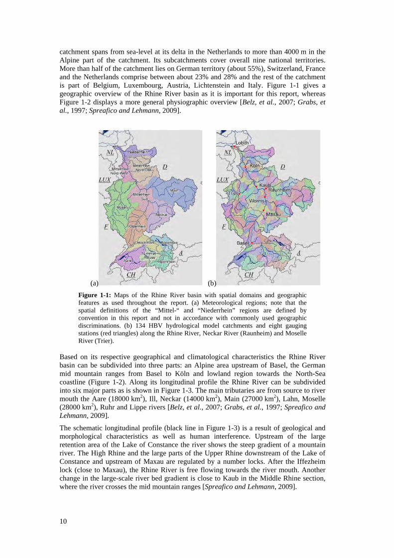
catchment spans from sea-level at its delta in the Netherlands to more than 4000 m in the Alpine part of the catchment. Its subcatchments cover overall nine national territories. More than half of the catchment lies on German territory (about 55%), Switzerland, France and the Netherlands comprise between about 23% and 28% and the rest of the catchment is part of Belgium, Luxembourg, Austria, Lichtenstein and Italy. Figure 1-1 gives a geographic overview of the Rhine River basin as it is important for this report, whereas Figure 1-2 displays a more general physiographic overview [Belz, et al., 2007; Grabs, et al., 1997; Spreafico and Lehmann, 2009].
(a) (b) Figure 1-1: Maps of the Rhine River basin with spatial domains and geographic features as used throughout the report. (a) Meteorological regions; note that the spatial definitions of the “Mittel-“ and “Niederrhein” regions are defined by convention in this report and not in accordance with commonly used geographic discriminations. (b) 134 HBV hydrological model catchments and eight gauging stations (red triangles) along the Rhine River, Neckar River (Raunheim) and Moselle River (Trier).
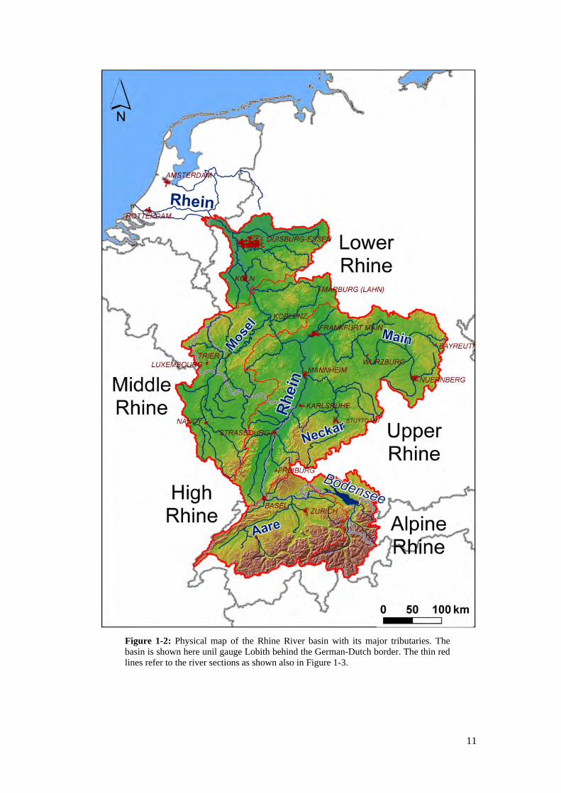
Based on its respective geographical and climatological characteristics the Rhine River basin can be subdivided into three parts: an Alpine area upstream of Basel, the German mid mountain ranges from Basel to Köln and lowland region towards the North-Sea coastline (Figure 1-2). Along its longitudinal profile the Rhine River can be subdivided into six major parts as is shown in Figure 1-3. The main tributaries are from source to river mouth the Aare (18000 km2), Ill, Neckar (14000 km2), Main (27000 km2), Lahn, Moselle (28000 km2), Ruhr and Lippe rivers [Belz, et al., 2007; Grabs, et al., 1997; Spreafico and Lehmann, 2009].
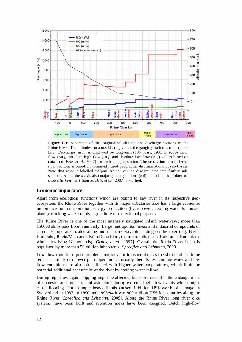
The schematic longitudinal profile (black line in Figure 1-3) is a result of geological and morphological characteristics as well as human interference. Upstream of the large retention area of the Lake of Constance the river shows the steep gradient of a mountain river. The High Rhine and the large parts of the Upper Rhine downstream of the Lake of Constance and upstream of Maxau are regulated by a number locks. After the Iffezheim lock (close to Maxau), the Rhine River is free flowing towards the river mouth. Another change in the large-scale river bed gradient is close to Kaub in the Middle Rhine section, where the river crosses the mid mountain ranges [Spreafico and Lehmann, 2009].
11
Figure 1-2: Physical map of the Rhine River basin with its major tributaries. The basin is shown here unil gauge Lobith behind the German-Dutch border. The thin red lines refer to the river sections as shown also in Figure 1-3.
12
Figure 1-3: Schematic of the longitudinal altitude and discharge sections of the Rhine River. The altitudes [m a.m.s.l.] are given as the gauging station datums (black line). Discharge [m3/s] is displayed by long-term (100 years, 1901 to 2000) mean flow (MQ), absolute high flow (HQ) and absolute low flow (NQ) values based on data from Belz, et al., 2007] for each gauging station. The separation into different river sections is based on commonly used geographic discriminations of sub-basins. Note that what is labelled “Alpine Rhine” can be discriminated into further sub-sections. Along the x-axis also major gauging stations (red) and tributaries (blue) are shown (in German). Source: Belz, et al. [2007], modified.
Economic importance Apart from ecological functions which are bound to any river in its respective geo-ecosystem, the Rhine River together with its major tributaries also has a large economic importance for transportation, energy production (hydropower, cooling water for power plants), drinking water supply, agriculture or recreational purposes.
The Rhine River is one of the most intensely navigated inland waterways; more than 150000 ships pass Lobith annually. Large metropolitan areas and industrial compounds of central Europe are located along and in many ways depending on the river (e.g. Basel, Karlsruhe, Rhein/Main area, Köln/Düsseldorf, the metropolis of the Ruhr area, Rotterdam, whole low-lying Netherlands) [Grabs, et al., 1997]. Overall the Rhein River basin is populated by more than 50 million inhabitants [Spreafico and Lehmann, 2009].
Low flow conditions pose problems not only for transportation as the ship-load has to be reduced, but also to power plant operators as usually there is less cooling water and low flow conditions are also often linked with higher water temperatures, which limit the potential additional heat uptake of the river by cooling water inflow.
During high flow again shipping might be affected, but more crucial is the endangerment of domestic and industrial infrastructure during extreme high flow events which might cause flooding. For example heavy floods caused 1 billion US$ worth of damage in Switzerland in 1987, in 1990 and 1993/94 it was 900 million US$ for countries along the Rhine River [Spreafico and Lehmann, 2009]. Along the Rhine River long river dike systems have been built and retention areas have been assigned. Dutch high-flow
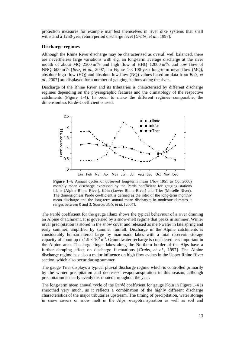
13
protection measures for example manifest themselves in river dike systems that shall withstand a 1250-year return period discharge level [Grabs, et al., 1997].
Discharge regimes Although the Rhine River discharge may be characterised as overall well balanced, there are nevertheless large variations with e.g. an long-term average discharge at the river mouth of about MQ=2500 m3/s and high flow of HHQ=12000 m3/s and low flow of NNQ=600 m3/s [Belz, et al., 2007]. In Figure 1-3 100-year long-term mean flow (MQ), absolute high flow (HQ) and absolute low flow (NQ) values based on data from Belz, et al., 2007] are displayed for a number of gauging stations along the river.
Discharge of the Rhine River and its tributaries is characterised by different discharge regimes depending on the physiographic features and the climatology of the respective catchments (Figure 1-4). In order to make the different regimes comparable, the dimensionless Pardé-Coefficient is used.
Figure 1-4: Annual cycles of observed long-term mean (Nov 1951 to Oct 2000) monthly mean discharge expressed by the Pardé coefficient for gauging stations Illanz (Alpine Rhine River), Köln (Lower Rhine River) and Trier (Moselle River). The dimensionless Pardé coefficient is defined as the ratio of the long-term monthly mean discharge and the long-term annual mean discharge; in moderate climates it ranges between 0 and 3. Source: Belz, et al. [2007].
The Pardé coefficient for the gauge Illanz shows the typical behaviour of a river draining an Alpine chatchment. It is governed by a snow-melt regime that peaks in summer. Winter nival precipitation is stored in the snow cover and released as melt-water in late spring and early summer, amplified by summer rainfall. Discharge in the Alpine catchments is considerably human-altered large by man-made lakes with a total reservoir storage capacity of about up to 1.9 × 10⁹ m3. Groundwater recharge is considered less important in the Alpine area. The large finger lakes along the Northern border of the Alps have a further damping effect on discharge fluctuations [Grabs, et al., 1997]. The Alpine discharge regime has also a major influence on high flow events in the Upper Rhine River section, which also occur during summer.
The gauge Trier displays a typical pluvial discharge regime which is controlled primarily by the winter precipitation and decreased evapotranspiration in this season, although precipitation is nearly evenly distributed throughout the year.
The long-term mean annual cycle of the Pardé coefficient for gauge Köln in Figure 1-4 is smoothed very much, as it reflects a combination of the highly different discharge characteristics of the major tributaries upstream. The timing of precipitation, water storage in snow covers or snow melt in the Alps, evapotranspiration as well as soil and
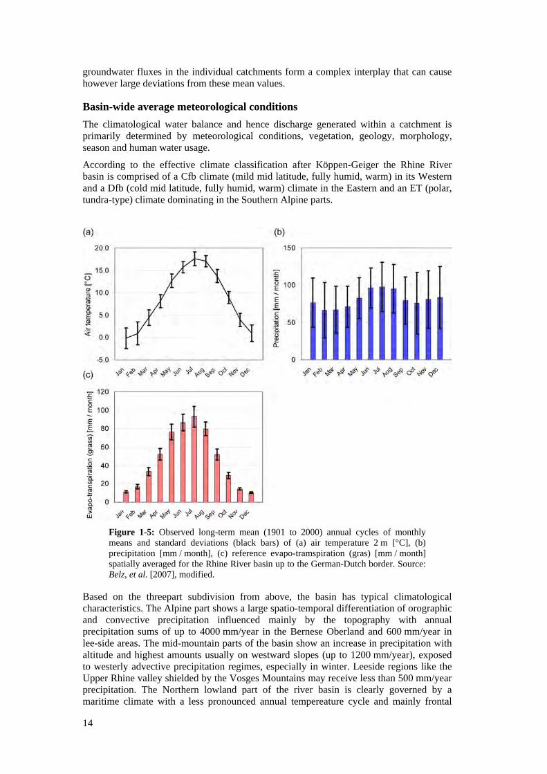
14
groundwater fluxes in the individual catchments form a complex interplay that can cause however large deviations from these mean values.
Basin-wide average meteorological conditions The climatological water balance and hence discharge generated within a catchment is primarily determined by meteorological conditions, vegetation, geology, morphology, season and human water usage.
According to the effective climate classification after Köppen-Geiger the Rhine River basin is comprised of a Cfb climate (mild mid latitude, fully humid, warm) in its Western and a Dfb (cold mid latitude, fully humid, warm) climate in the Eastern and an ET (polar, tundra-type) climate dominating in the Southern Alpine parts.
Figure 1-5: Observed long-term mean (1901 to 2000) annual cycles of monthly means and standard deviations (black bars) of (a) air temperature 2 m [°C], (b) precipitation [mm / month], (c) reference evapo-tramspiration (gras) [mm / month] spatially averaged for the Rhine River basin up to the German-Dutch border. Source: Belz, et al. [2007], modified.
Based on the threepart subdivision from above, the basin has typical climatological characteristics. The Alpine part shows a large spatio-temporal differentiation of orographic and convective precipitation influenced mainly by the topography with annual precipitation sums of up to 4000 mm/year in the Bernese Oberland and 600 mm/year in lee-side areas. The mid-mountain parts of the basin show an increase in precipitation with altitude and highest amounts usually on westward slopes (up to 1200 mm/year), exposed to westerly advective precipitation regimes, especially in winter. Leeside regions like the Upper Rhine valley shielded by the Vosges Mountains may receive less than 500 mm/year precipitation. The Northern lowland part of the river basin is clearly governed by a maritime climate with a less pronounced annual tempereature cycle and mainly frontal
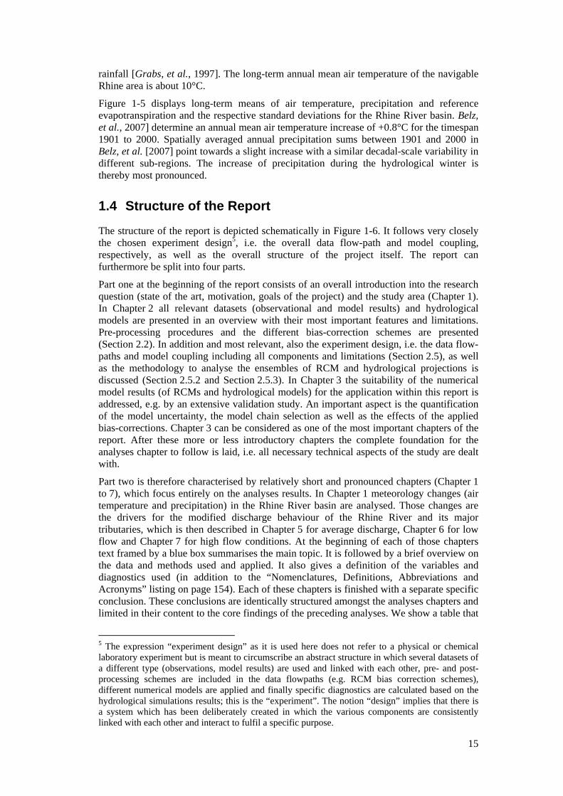
15
rainfall [Grabs, et al., 1997]. The long-term annual mean air temperature of the navigable Rhine area is about 10°C.
Figure 1-5 displays long-term means of air temperature, precipitation and reference evapotranspiration and the respective standard deviations for the Rhine River basin. Belz, et al., 2007] determine an annual mean air temperature increase of +0.8°C for the timespan 1901 to 2000. Spatially averaged annual precipitation sums between 1901 and 2000 in Belz, et al. [2007] point towards a slight increase with a similar decadal-scale variability in different sub-regions. The increase of precipitation during the hydrological winter is thereby most pronounced.
1.4 Structure of the Report
The structure of the report is depicted schematically in Figure 1-6. It follows very closely the chosen experiment design5, i.e. the overall data flow-path and model coupling, respectively, as well as the overall structure of the project itself. The report can furthermore be split into four parts.
Part one at the beginning of the report consists of an overall introduction into the research question (state of the art, motivation, goals of the project) and the study area (Chapter 1). In Chapter 2 all relevant datasets (observational and model results) and hydrological models are presented in an overview with their most important features and limitations. Pre-processing procedures and the different bias-correction schemes are presented (Section 2.2). In addition and most relevant, also the experiment design, i.e. the data flow-paths and model coupling including all components and limitations (Section 2.5), as well as the methodology to analyse the ensembles of RCM and hydrological projections is discussed (Section 2.5.2 and Section 2.5.3). In Chapter 3 the suitability of the numerical model results (of RCMs and hydrological models) for the application within this report is addressed, e.g. by an extensive validation study. An important aspect is the quantification of the model uncertainty, the model chain selection as well as the effects of the applied bias-corrections. Chapter 3 can be considered as one of the most important chapters of the report. After these more or less introductory chapters the complete foundation for the analyses chapter to follow is laid, i.e. all necessary technical aspects of the study are dealt with.
Part two is therefore characterised by relatively short and pronounced chapters (Chapter 1 to 7), which focus entirely on the analyses results. In Chapter 1 meteorology changes (air temperature and precipitation) in the Rhine River basin are analysed. Those changes are the drivers for the modified discharge behaviour of the Rhine River and its major tributaries, which is then described in Chapter 5 for average discharge, Chapter 6 for low flow and Chapter 7 for high flow conditions. At the beginning of each of those chapters text framed by a blue box summarises the main topic. It is followed by a brief overview on the data and methods used and applied. It also gives a definition of the variables and diagnostics used (in addition to the “Nomenclatures, Definitions, Abbreviations and Acronyms” listing on page 154). Each of these chapters is finished with a separate specific conclusion. These conclusions are identically structured amongst the analyses chapters and limited in their content to the core findings of the preceding analyses. We show a table that
5 The expression “experiment design” as it is used here does not refer to a physical or chemical laboratory experiment but is meant to circumscribe an abstract structure in which several datasets of a different type (observations, model results) are used and linked with each other, pre- and post-processing schemes are included in the data flowpaths (e.g. RCM bias correction schemes), different numerical models are applied and finally specific diagnostics are calculated based on the hydrological simulations results; this is the “experiment”. The notion “design” implies that there is a system which has been deliberately created in which the various components are consistently linked with each other and interact to fulfil a specific purpose.
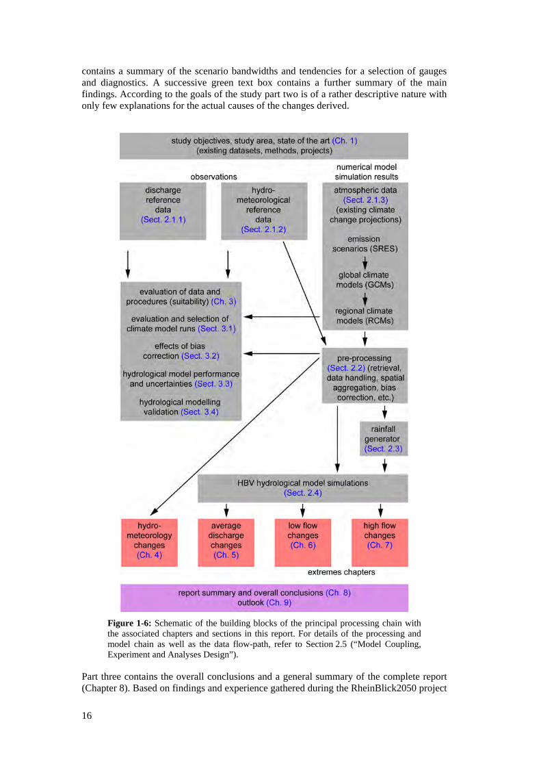
16
contains a summary of the scenario bandwidths and tendencies for a selection of gauges and diagnostics. A successive green text box contains a further summary of the main findings. According to the goals of the study part two is of a rather descriptive nature with only few explanations for the actual causes of the changes derived.
Figure 1-6: Schematic of the building blocks of the principal processing chain with the associated chapters and sections in this report. For details of the processing and model chain as well as the data flow-path, refer to Section 2.5 (“Model Coupling, Experiment and Analyses Design”).
Part three contains the overall conclusions and a general summary of the complete report (Chapter 8). Based on findings and experience gathered during the RheinBlick2050 project

17
we also identify issues in the outlook in Chapter 9 that might pose future research questions.
Part four consists of the appendix which contains information on the definition of the diagnostics applied in Chapter 1 to Chapter 7 (Appendix A), followed by an extensive overview of all currently available (to the project group members) regional climate change projections (Appendix B) and a tabulated detailed overview on the hydrological model features (Appendix C) as well as well as validation and intercomparison tables for hydrological models (Appendix D) accompanying Section 3.3. The remainder of the appendix is add-ons to the analyses chapters. In case of the hydrometeorology changes these are more detailed plots for individual subsets of air temperature and precipitation changes; for Chapter 7 on high flow additional return level plots are shown.

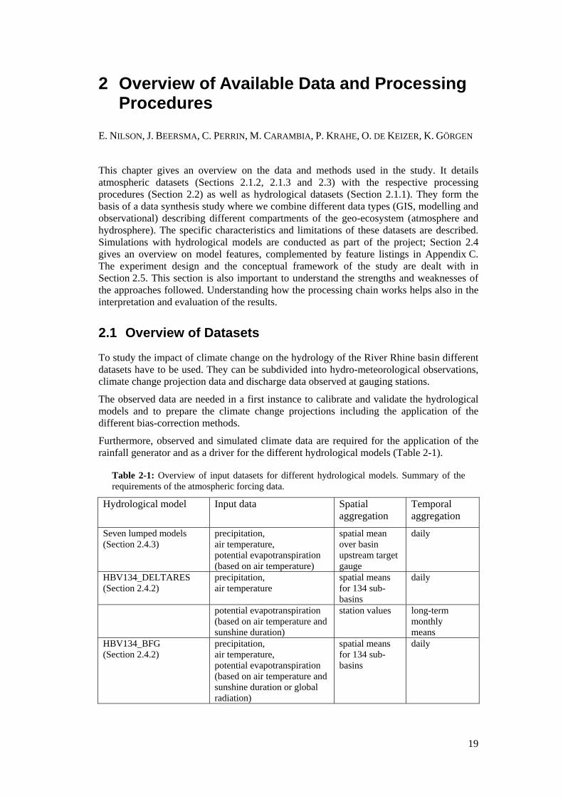
19
2 Overview of Available Data and Processing Procedures
E. NILSON, J. BEERSMA, C. PERRIN, M. CARAMBIA, P. KRAHE, O. DE KEIZER, K. GÖRGEN
This chapter gives an overview on the data and methods used in the study. It details atmospheric datasets (Sections 2.1.2, 2.1.3 and 2.3) with the respective processing procedures (Section 2.2) as well as hydrological datasets (Section 2.1.1). They form the basis of a data synthesis study where we combine different data types (GIS, modelling and observational) describing different compartments of the geo-ecosystem (atmosphere and hydrosphere). The specific characteristics and limitations of these datasets are described. Simulations with hydrological models are conducted as part of the project; Section 2.4 gives an overview on model features, complemented by feature listings in Appendix C. The experiment design and the conceptual framework of the study are dealt with in Section 2.5. This section is also important to understand the strengths and weaknesses of the approaches followed. Understanding how the processing chain works helps also in the interpretation and evaluation of the results.
2.1 Overview of Datasets
To study the impact of climate change on the hydrology of the River Rhine basin different datasets have to be used. They can be subdivided into hydro-meteorological observations, climate change projection data and discharge data observed at gauging stations.
The observed data are needed in a first instance to calibrate and validate the hydrological models and to prepare the climate change projections including the application of the different bias-correction methods.
Furthermore, observed and simulated climate data are required for the application of the rainfall generator and as a driver for the different hydrological models (Table 2-1).
Table 2-1: Overview of input datasets for different hydrological models. Summary of the requirements of the atmospheric forcing data.
Hydrological model Input data Spatial aggregation
Temporal aggregation
Seven lumped models (Section 2.4.3)
precipitation, air temperature, potential evapotranspiration (based on air temperature)
spatial mean over basin upstream target gauge
daily
HBV134_DELTARES (Section 2.4.2)
precipitation, air temperature
spatial means for 134 sub-basins
daily
potential evapotranspiration (based on air temperature and sunshine duration)
station values long-term monthly means
HBV134_BFG (Section 2.4.2)
precipitation, air temperature, potential evapotranspiration (based on air temperature and sunshine duration or global radiation)
spatial means for 134 sub-basins
daily
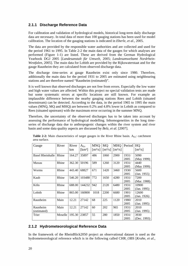
20
2.1.1 Discharge Reference Data
For calibration and validation of hydrological models, historical long-term daily discharge data are necessary. In total data of more than 100 gauging stations has been used for model calibration. The location of the gauging stations is indicated in Eberle, et al., 2005.
The data are provided by the responsible water authorities and are collected and used for the period 1961 to 1995. In Table 2-2 the main data of the gauges for which analyses are performed (Figure 1-1) are listed. These are derived from the German Hydrological Yearbook DGJ 2005 [Landesanstalt für Umwelt, 2005; Landesumweltamt Nordrhein-Westfalen, 2005]. The main data for Lobith are provided by the Rijkswaterstaat and for the gauge Raunheim they are calculated from observed discharge data.
The discharge time-series at gauge Raunheim exist only since 1980. Therefore, additionally the main data for the period 1931 to 2005 are estimated using neighbouring stations and are therefore named “Raunheim (estimated)”.
It is well known that observed discharges are not free from errors. Especially the low water and high water values are affected. Within this project no special validation tests are made but some systematic errors at specific locations are still known. For example an implausible difference between the nearby gauging stations Rees and Lobith (situated downstream) can be detected. According to the data, in the period 1965 to 1995 the main values (MNQ, MQ and MHQ) are between 0.2% and 4.8% lower in Lobith as compared to Rees (situated upstream) with the maximum error occurring in the summer MNQ.
Therefore, the uncertainty of the observed discharges has to be taken into account by assessing the performance of hydrological modelling. Inhomogeneities in the long time-series of discharge data due to anthropogenic changes within the river system and river basin and some data quality aspects are discussed by Belz, et al. [2007].
Table 2-2: Main characteristics of target gauges in the River Rhine basin. AEo: catchment area surface.
Gauge River River km
AEo [km²]
MNQ [m³/s]
MQ [m³/s]
MHQ [m³/s]
Period HQ [m³/s]
Basel Rheinhalle Rhine 164.27 35897 486 1060 2900 1931/ 2005
5090 (May 1999)
Maxau Rhine 362.30 50196 589 1260 3120 1931/ 2005
4440 (May 1999)
Worms Rhine 443.40 68827 671 1420 3460 1930/ 2005
5600 (Jan. 1955)
Kaub Rhine 546.20 103488 772 1650 4280 1931/ 2005
7200 (Mar. 1988)
Köln Rhine 688.00 144232 942 2120 6480 1931/ 2005
10900 (Jan. 1995)
Lobith Rhine 865.00 160800 1018 2200 6680 1901/ 2005
12600 (Jan. 1926)
Raunheim Main 12.21 27142 68 225 1120 1980/ 2005
2010 (Jan. 1995)
Raunheim (estimated)
Main 12.21 27142 60 202 965 1931/ 2005
2010 (Jan. 1995)
Trier Moselle 195.30 23857 55 280 1850 1931/ 2005
3930 (Dec. 1993)
2.1.2 Hydrometeorological Reference Data
In the framework of the RheinBlick2050 project an observational dataset is used as the hydrometeorological reference which is in the following called CHR_OBS [Krahe, et al.,
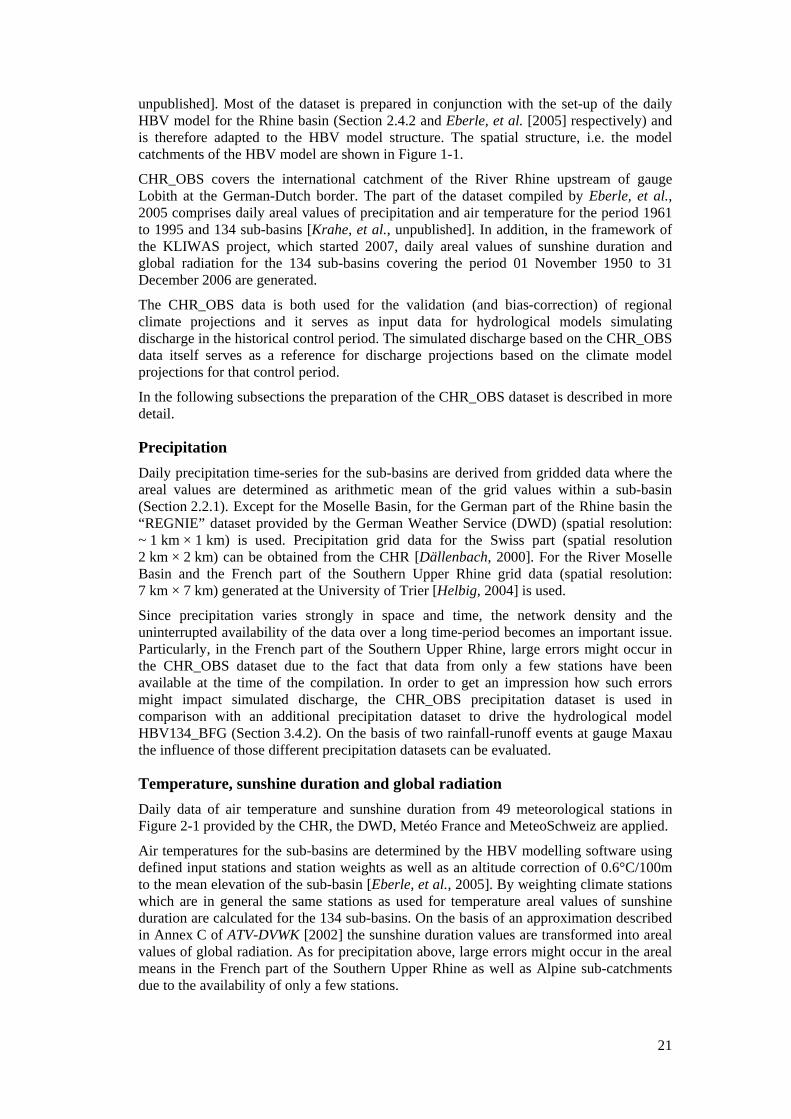
21
unpublished]. Most of the dataset is prepared in conjunction with the set-up of the daily HBV model for the Rhine basin (Section 2.4.2 and Eberle, et al. [2005] respectively) and is therefore adapted to the HBV model structure. The spatial structure, i.e. the model catchments of the HBV model are shown in Figure 1-1.
CHR_OBS covers the international catchment of the River Rhine upstream of gauge Lobith at the German-Dutch border. The part of the dataset compiled by Eberle, et al., 2005 comprises daily areal values of precipitation and air temperature for the period 1961 to 1995 and 134 sub-basins [Krahe, et al., unpublished]. In addition, in the framework of the KLIWAS project, which started 2007, daily areal values of sunshine duration and global radiation for the 134 sub-basins covering the period 01 November 1950 to 31 December 2006 are generated.
The CHR_OBS data is both used for the validation (and bias-correction) of regional climate projections and it serves as input data for hydrological models simulating discharge in the historical control period. The simulated discharge based on the CHR_OBS data itself serves as a reference for discharge projections based on the climate model projections for that control period.
In the following subsections the preparation of the CHR_OBS dataset is described in more detail.
Precipitation Daily precipitation time-series for the sub-basins are derived from gridded data where the areal values are determined as arithmetic mean of the grid values within a sub-basin (Section 2.2.1). Except for the Moselle Basin, for the German part of the Rhine basin the “REGNIE” dataset provided by the German Weather Service (DWD) (spatial resolution: ~ 1 km × 1 km) is used. Precipitation grid data for the Swiss part (spatial resolution 2 km × 2 km) can be obtained from the CHR [Dällenbach, 2000]. For the River Moselle Basin and the French part of the Southern Upper Rhine grid data (spatial resolution: 7 km × 7 km) generated at the University of Trier [Helbig, 2004] is used.
Since precipitation varies strongly in space and time, the network density and the uninterrupted availability of the data over a long time-period becomes an important issue. Particularly, in the French part of the Southern Upper Rhine, large errors might occur in the CHR_OBS dataset due to the fact that data from only a few stations have been available at the time of the compilation. In order to get an impression how such errors might impact simulated discharge, the CHR_OBS precipitation dataset is used in comparison with an additional precipitation dataset to drive the hydrological model HBV134_BFG (Section 3.4.2). On the basis of two rainfall-runoff events at gauge Maxau the influence of those different precipitation datasets can be evaluated.
Temperature, sunshine duration and global radiation Daily data of air temperature and sunshine duration from 49 meteorological stations in Figure 2-1 provided by the CHR, the DWD, Metéo France and MeteoSchweiz are applied.
Air temperatures for the sub-basins are determined by the HBV modelling software using defined input stations and station weights as well as an altitude correction of 0.6°C/100m to the mean elevation of the sub-basin [Eberle, et al., 2005]. By weighting climate stations which are in general the same stations as used for temperature areal values of sunshine duration are calculated for the 134 sub-basins. On the basis of an approximation described in Annex C of ATV-DVWK [2002] the sunshine duration values are transformed into areal values of global radiation. As for precipitation above, large errors might occur in the areal means in the French part of the Southern Upper Rhine as well as Alpine sub-catchments due to the availability of only a few stations.
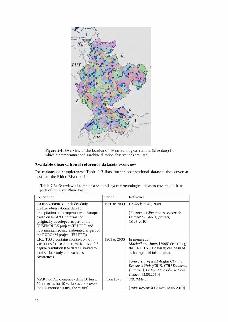
22
Figure 2-1: Overview of the location of 49 meteorological stations (blue dots) from which air temperature and sunshine duration observations are used.
Available observational reference datasets overview For reasons of completeness Table 2-3 lists further observational datasets that cover at least part the Rhine River basin.
Table 2-3: Overview of some observational hydrometeorological datasets covering at least parts of the River Rhine Basin.
Description Period Reference
E-OBS version 3.0 includes daily gridded observational data for precipitation and temperature in Europe based on ECA&D information (originally developed as part of the ENSEMBLES project (EU-FP6) and now maintained and elaborated as part of the EURO4M project (EU-FP7))
1950 to 2009 Haylock, et al., 2008 [European Climate Assessment & Dataset (ECA&D) project, 18.05.2010]
CRU TS3.0 contains month-by-month variations for 10 climate variables at 0.5 degree resolution (the data is limited to land surface only and excludes Antarctica)
1901 to 2006 In preparation. Mitchell and Jones [2005] describing the CRU TS 2.1 dataset; can be used as background information. [University of East Anglia Climate Research Unit (CRU). CRU Datasets, [Internet]. British Atmospheric Data Centre, 18.05.2010]
MARS-STAT comprises daily 50 km x 50 km grids for 10 variables and covers the EU member states, the central
From 1975 JRC/MARS, [Joint Research Centre, 18.05.2010]
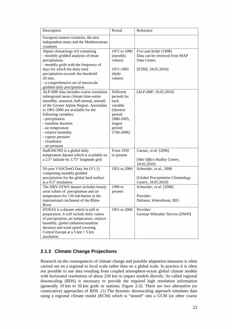
23
Description Period Reference
European eastern countries, the new independent states and the Mediterranean countries Alpine climatology 4.0 containing - monthly gridded analyses of mean precipitation, - monthly grids with the frequency of days for which the daily total precipitation exceeds the threshold 20 mm, - a comprehensive set of mesoscale gridded daily precipitation
1971 to 1990 (monthly values) 1971-1992 (daily values)
Frei and Schär [1998] Data can be retrieved from MAP Data Centre. [ETHZ, 18.05.2010]
ALP-IMP data includes coarse resolution subregional mean climate time-series (monthly, seasonal, half-annual, annual) of the Greater Alpine Region. Anomalies to 1901-2000 are available for the following variables: - precipitation - sunshine duration - air temperature - relative humidity - vapour pressure - cloudiness - air pressure
Different periods for each variable (shortest period: 1880-2005, largest period: 1760-2006)
[ALP-IMP, 18.05.2010]
HadGHCND is a global daily temperature dataset which is available on a 2.5° latitude by 3.75° longitude grid
From 1950 to present
Caesar, et al. [2006] [Met Office Hadley Centre, 18.05.2010]
50-year VASClimO Data Set (V1.1) comprising monthly gridded precipitation for the global land surface at a 0.5° resolution
1951 to 2000 Schneider, et al., 2008 [Global Precipitation Climatology Centre, 18.05.2010]
The HBV-FEWS dataset includes hourly areal values of precipitation and air temperature for 134 sub-basins in the international catchment of the Rhine River
1996 to present
Schneider, et al. [2008] Provider: Deltares, Waterdienst, BfG
HYRAS is a dataset which is still in preparation. It will include daily values of precipitation, air temperature, relative humidity, global radiation/sunshine duration and wind speed covering Central Europe at a 5 km × 5 km resolution
1951 to 2006 Provider: German Wheather Service (DWD)
2.1.3 Climate Change Projections
Research on the consequences of climate change and possible adaptation measures is often carried out on a regional to local scale rather than on a global scale. In practice it is often not possible to use data resulting from coupled atmosphere-ocean global climate models with horizontal resolutions of about 250 km in impact models directly. So called regional downscaling (RDS) is necessary to provide the required high resolution information (generally 10 km to 50 km grids or stations; Figure 2-2). There are two alternative (or consecutive) approaches of RDS. (1) The dynamic downscaling approach simulates data using a regional climate model (RCM) which is “nested” into a GCM (or other coarse
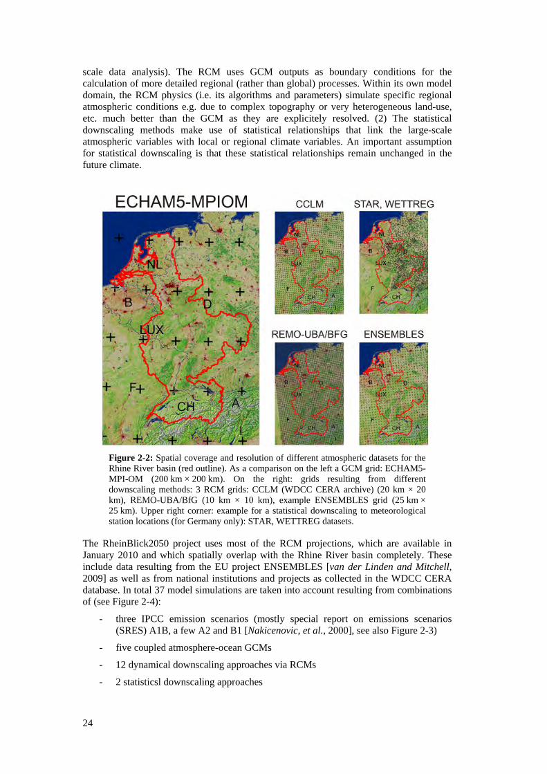
24
scale data analysis). The RCM uses GCM outputs as boundary conditions for the calculation of more detailed regional (rather than global) processes. Within its own model domain, the RCM physics (i.e. its algorithms and parameters) simulate specific regional atmospheric conditions e.g. due to complex topography or very heterogeneous land-use, etc. much better than the GCM as they are explicitely resolved. (2) The statistical downscaling methods make use of statistical relationships that link the large-scale atmospheric variables with local or regional climate variables. An important assumption for statistical downscaling is that these statistical relationships remain unchanged in the future climate.
Figure 2-2: Spatial coverage and resolution of different atmospheric datasets for the Rhine River basin (red outline). As a comparison on the left a GCM grid: ECHAM5-MPI-OM (200 km × 200 km). On the right: grids resulting from different downscaling methods: 3 RCM grids: CCLM (WDCC CERA archive) (20 km × 20 km), REMO-UBA/BfG (10 km × 10 km), example ENSEMBLES grid (25 km × 25 km). Upper right corner: example for a statistical downscaling to meteorological station locations (for Germany only): STAR, WETTREG datasets.
The RheinBlick2050 project uses most of the RCM projections, which are available in January 2010 and which spatially overlap with the Rhine River basin completely. These include data resulting from the EU project ENSEMBLES [van der Linden and Mitchell, 2009] as well as from national institutions and projects as collected in the WDCC CERA database. In total 37 model simulations are taken into account resulting from combinations of (see Figure 2-4):
- three IPCC emission scenarios (mostly special report on emissions scenarios (SRES) A1B, a few A2 and B1 [Nakicenovic, et al., 2000], see also Figure 2-3)
- five coupled atmosphere-ocean GCMs
- 12 dynamical downscaling approaches via RCMs
- 2 statisticsl downscaling approaches
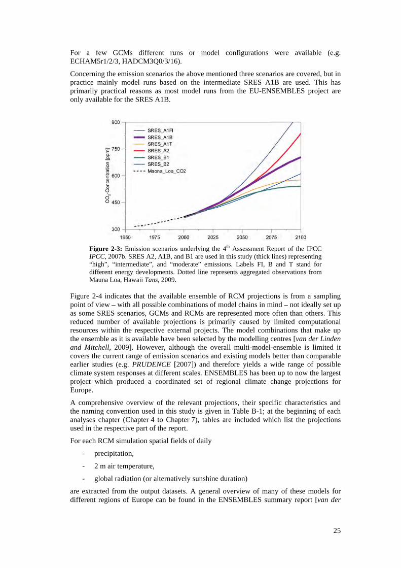
25
For a few GCMs different runs or model configurations were available (e.g. ECHAM5r1/2/3, HADCM3Q0/3/16).
Concerning the emission scenarios the above mentioned three scenarios are covered, but in practice mainly model runs based on the intermediate SRES A1B are used. This has primarily practical reasons as most model runs from the EU-ENSEMBLES project are only available for the SRES A1B.
Figure 2-3: Emission scenarios underlying the 4th Assessment Report of the IPCC IPCC, 2007b. SRES A2, A1B, and B1 are used in this study (thick lines) representing “high”, “intermediate”, and “moderate” emissions. Labels FI, B and T stand for different energy developments. Dotted line represents aggregated observations from Mauna Loa, Hawaii Tans, 2009.
Figure 2-4 indicates that the available ensemble of RCM projections is from a sampling point of view – with all possible combinations of model chains in mind – not ideally set up as some SRES scenarios, GCMs and RCMs are represented more often than others. This reduced number of available projections is primarily caused by limited computational resources within the respective external projects. The model combinations that make up the ensemble as it is available have been selected by the modelling centres [van der Linden and Mitchell, 2009]. However, although the overall multi-model-ensemble is limited it covers the current range of emission scenarios and existing models better than comparable earlier studies (e.g. PRUDENCE [2007]) and therefore yields a wide range of possible climate system responses at different scales. ENSEMBLES has been up to now the largest project which produced a coordinated set of regional climate change projections for Europe.
A comprehensive overview of the relevant projections, their specific characteristics and the naming convention used in this study is given in Table B-1; at the beginning of each analyses chapter (Chapter 4 to Chapter 7), tables are included which list the projections used in the respective part of the report.
For each RCM simulation spatial fields of daily
- precipitation,
- 2 m air temperature,
- global radiation (or alternatively sunshine duration)
are extracted from the output datasets. A general overview of many of these models for different regions of Europe can be found in the ENSEMBLES summary report [van der
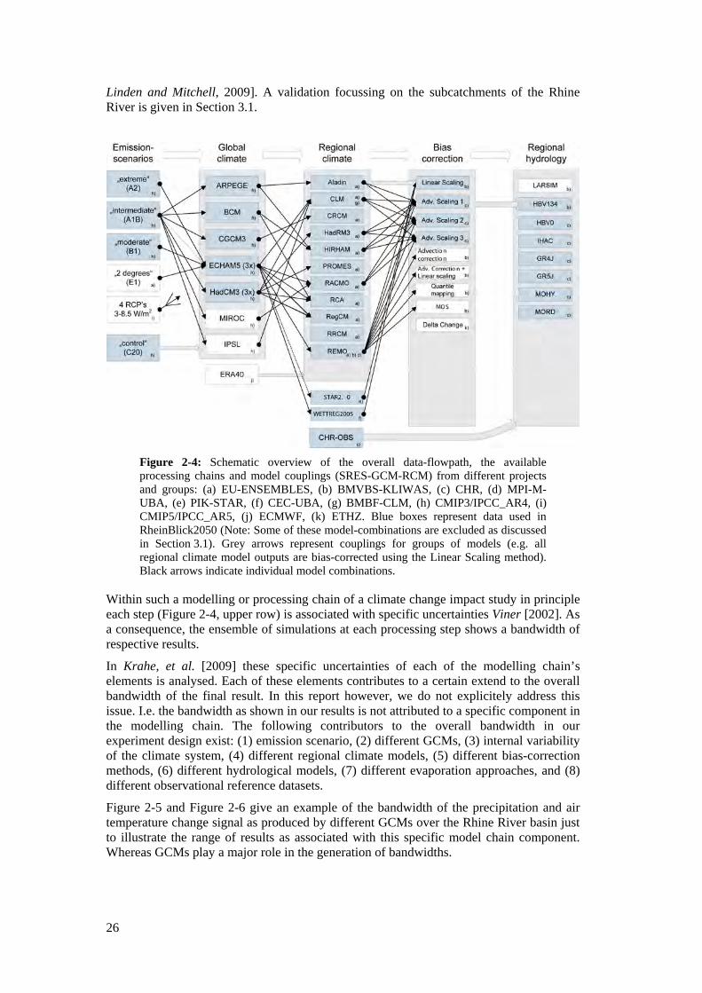
26
Linden and Mitchell, 2009]. A validation focussing on the subcatchments of the Rhine River is given in Section 3.1.
Figure 2-4: Schematic overview of the overall data-flowpath, the available processing chains and model couplings (SRES-GCM-RCM) from different projects and groups: (a) EU-ENSEMBLES, (b) BMVBS-KLIWAS, (c) CHR, (d) MPI-M-UBA, (e) PIK-STAR, (f) CEC-UBA, (g) BMBF-CLM, (h) CMIP3/IPCC_AR4, (i) CMIP5/IPCC_AR5, (j) ECMWF, (k) ETHZ. Blue boxes represent data used in RheinBlick2050 (Note: Some of these model-combinations are excluded as discussed in Section 3.1). Grey arrows represent couplings for groups of models (e.g. all regional climate model outputs are bias-corrected using the Linear Scaling method). Black arrows indicate individual model combinations.
Within such a modelling or processing chain of a climate change impact study in principle each step (Figure 2-4, upper row) is associated with specific uncertainties Viner [2002]. As a consequence, the ensemble of simulations at each processing step shows a bandwidth of respective results.
In Krahe, et al. [2009] these specific uncertainties of each of the modelling chain’s elements is analysed. Each of these elements contributes to a certain extend to the overall bandwidth of the final result. In this report however, we do not explicitely address this issue. I.e. the bandwidth as shown in our results is not attributed to a specific component in the modelling chain. The following contributors to the overall bandwidth in our experiment design exist: (1) emission scenario, (2) different GCMs, (3) internal variability of the climate system, (4) different regional climate models, (5) different bias-correction methods, (6) different hydrological models, (7) different evaporation approaches, and (8) different observational reference datasets.
Figure 2-5 and Figure 2-6 give an example of the bandwidth of the precipitation and air temperature change signal as produced by different GCMs over the Rhine River basin just to illustrate the range of results as associated with this specific model chain component. Whereas GCMs play a major role in the generation of bandwidths.
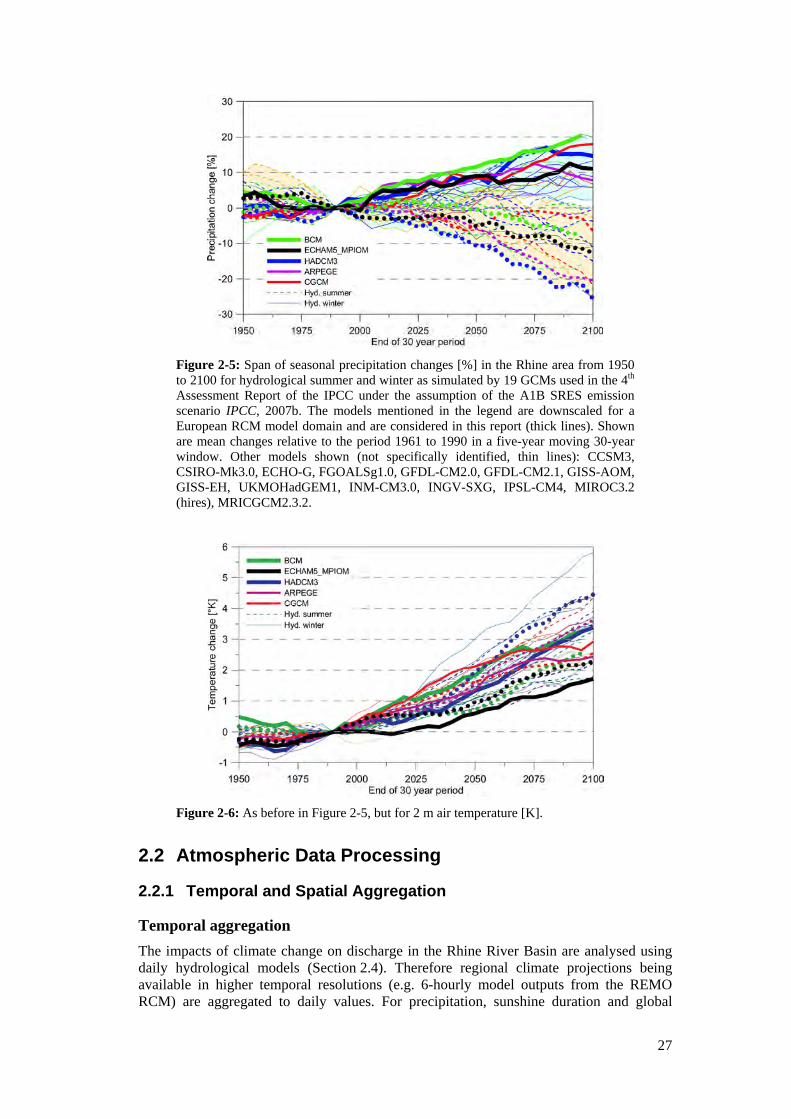
27
Figure 2-5: Span of seasonal precipitation changes [%] in the Rhine area from 1950 to 2100 for hydrological summer and winter as simulated by 19 GCMs used in the 4th Assessment Report of the IPCC under the assumption of the A1B SRES emission scenario IPCC, 2007b. The models mentioned in the legend are downscaled for a European RCM model domain and are considered in this report (thick lines). Shown are mean changes relative to the period 1961 to 1990 in a five-year moving 30-year window. Other models shown (not specifically identified, thin lines): CCSM3, CSIRO-Mk3.0, ECHO-G, FGOALSg1.0, GFDL-CM2.0, GFDL-CM2.1, GISS-AOM, GISS-EH, UKMOHadGEM1, INM-CM3.0, INGV-SXG, IPSL-CM4, MIROC3.2 (hires), MRICGCM2.3.2.
Figure 2-6: As before in Figure 2-5, but for 2 m air temperature [K].
2.2 Atmospheric Data Processing
2.2.1 Temporal and Spatial Aggregation
Temporal aggregation The impacts of climate change on discharge in the Rhine River Basin are analysed using daily hydrological models (Section 2.4). Therefore regional climate projections being available in higher temporal resolutions (e.g. 6-hourly model outputs from the REMO RCM) are aggregated to daily values. For precipitation, sunshine duration and global
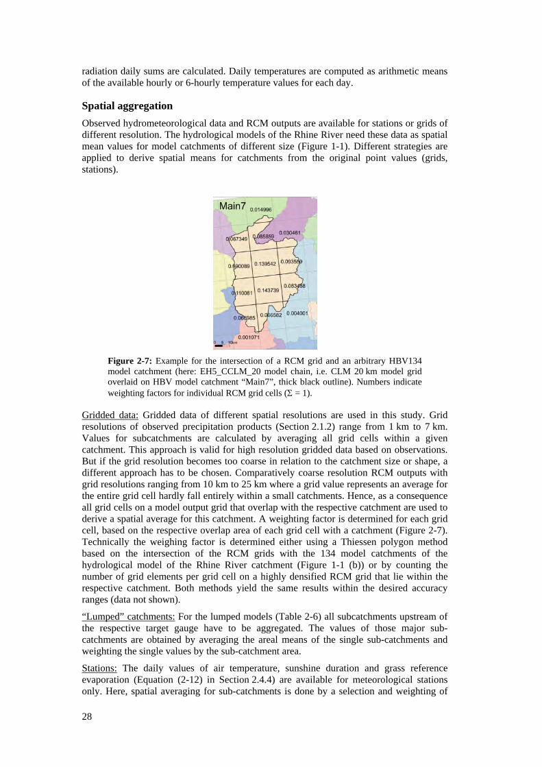
28
radiation daily sums are calculated. Daily temperatures are computed as arithmetic means of the available hourly or 6-hourly temperature values for each day.
Spatial aggregation Observed hydrometeorological data and RCM outputs are available for stations or grids of different resolution. The hydrological models of the Rhine River need these data as spatial mean values for model catchments of different size (Figure 1-1). Different strategies are applied to derive spatial means for catchments from the original point values (grids, stations).
Figure 2-7: Example for the intersection of a RCM grid and an arbitrary HBV134 model catchment (here: EH5_CCLM_20 model chain, i.e. CLM 20 km model grid overlaid on HBV model catchment “Main7”, thick black outline). Numbers indicate weighting factors for individual RCM grid cells (Σ = 1).
Gridded data: Gridded data of different spatial resolutions are used in this study. Grid resolutions of observed precipitation products (Section 2.1.2) range from 1 km to 7 km. Values for subcatchments are calculated by averaging all grid cells within a given catchment. This approach is valid for high resolution gridded data based on observations. But if the grid resolution becomes too coarse in relation to the catchment size or shape, a different approach has to be chosen. Comparatively coarse resolution RCM outputs with grid resolutions ranging from 10 km to 25 km where a grid value represents an average for the entire grid cell hardly fall entirely within a small catchments. Hence, as a consequence all grid cells on a model output grid that overlap with the respective catchment are used to derive a spatial average for this catchment. A weighting factor is determined for each grid cell, based on the respective overlap area of each grid cell with a catchment (Figure 2-7). Technically the weighing factor is determined either using a Thiessen polygon method based on the intersection of the RCM grids with the 134 model catchments of the hydrological model of the Rhine River catchment (Figure 1-1 (b)) or by counting the number of grid elements per grid cell on a highly densified RCM grid that lie within the respective catchment. Both methods yield the same results within the desired accuracy ranges (data not shown).
“Lumped” catchments: For the lumped models (Table 2-6) all subcatchments upstream of the respective target gauge have to be aggregated. The values of those major sub-catchments are obtained by averaging the areal means of the single sub-catchments and weighting the single values by the sub-catchment area.
Stations: The daily values of air temperature, sunshine duration and grass reference evaporation (Equation (2-12) in Section 2.4.4) are available for meteorological stations only. Here, spatial averaging for sub-catchments is done by a selection and weighting of
29
stations (Section 2.1.2 and Section 2.4.4) based on expert knowledge. With this approach regional hydrometeorological characteristics of the Rhine River basin (e.g. meteorological divides, uniform regions) can be accounted for (data not shown).
As a result of the temporal and spatial aggregation, uniform datasets with consistent characteristics are available
- for precipitation, air temperature and global radiation (or sunshine duration),
- based on observations and RCM simulations,
- for 134 subcatchments of the River Rhine basin from the Alps to Lobith,
- at a daily resolution.
These data are then further relayed in the processing chain (Section 2.5) in terms of bias-correction (Section 2.2.2), calculation of evaporation (Section 2.4.4) and time-series generation (Section 2.3) as well as discharge simulation (Section 2.4).
2.2.2 Bias-Correction Methods
This subsection gives general information, why bias-correction is a necessary processing step when dealing with regional climate model outputs. It gives an overview of different bias-correction methods and describes the methods selected for this study.
Although the RCMs and the GCMs that drive the RCMs are the current state-of-the-art models to simulate the highly complex climate system, it is well known that these models suffer from imperfections. These imperfections are largely related to (a) incomplete knowledge of certain processes in the atmosphere and ocean, and (b) necessary limitations of the spatial and temporal resolution because of limited computational resources (even on state-of-the-art earth-system modelling high performance computing systems).
As a consequence of the incomplete representation of the climate system, meteorological variables simulated by RCMs cannot be expected to reproduce observed values exactly. In fact, the control experiments, for a certain historical period, show that all climate models deviate more or less from observations in that period (Section 3.1). Since the ultimate goal here is to couple the simulated climatic time-series to hydrological models of the Rhine to determine the (future) change in various Rhine discharge characteristics such climatic biases are undesired. Quite often the biases are so large, that it becomes unreasonable to use the simulated data as input to climate impact models of natural systems, e.g. hydrological models. With a large bias in e.g. precipitation the hydrological model will operate in the wrong “regime” and will therefore very likely give a wrong sensitivity to (future) climate change (in particular when the response is highly non-linear). Similar effects can be expected from a temperature bias since e.g. a correct accumulation and melt of snow sensitively depends on a correct reproduction of the air temperature (in particular in the Alpine region). In addition, evaporation also depends on temperature, in particular during summer.
Those biases are caused partly by the RCM and partly by the driving GCM. The individual bias of the RCMs can be tested by driving them with “observed” fields such as e.g. ERA40 (e.g. Bülow, et al. [2009]; Arnold, et al. [2009]). In this study we focus on the overall bias of the different GCM-RCM combinations summarised in Section 2.1.3.
Despite of the bias, all climate models include “knowledge” about the dynamics of the climate system and how future conditions can evolve. They represent the only source of information about possible consequences of future greenhouse gas emissions as suggested by the IPCC [Nakicenovic, et al., 2000]. In order to make use of this knowledge in climate impact research several bias-correction methods have been developed during the recent years.
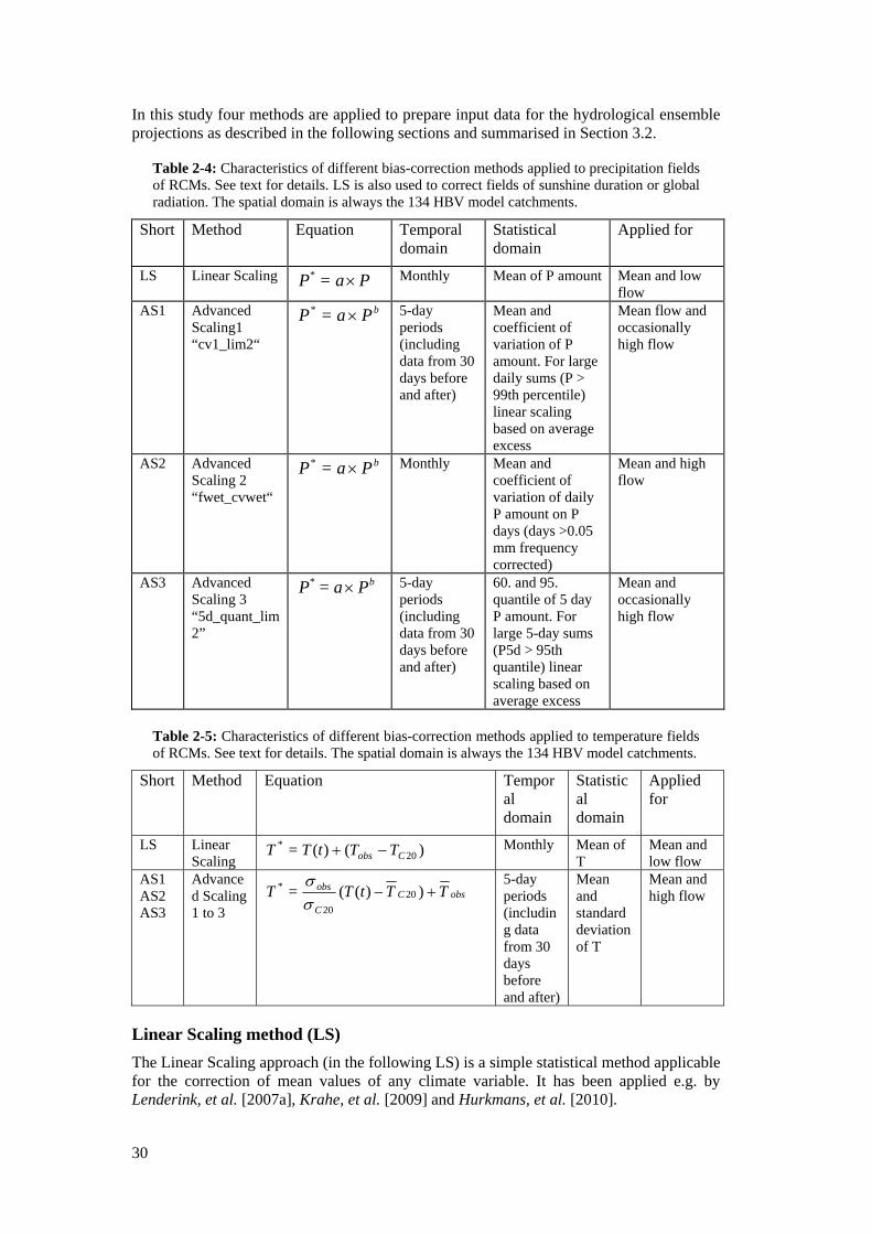
30
In this study four methods are applied to prepare input data for the hydrological ensemble projections as described in the following sections and summarised in Section 3.2.
Table 2-4: Characteristics of different bias-correction methods applied to precipitation fields of RCMs. See text for details. LS is also used to correct fields of sunshine duration or global radiation. The spatial domain is always the 134 HBV model catchments.
Short Method Equation Temporal domain
Statistical domain
Applied for
LS Linear Scaling Pa=P ×* Monthly Mean of P amount Mean and low flow
AS1 Advanced Scaling1 “cv1_lim2“
bPa=P ×*
5-day periods (including data from 30 days before and after)
Mean and coefficient of variation of P amount. For large daily sums (P > 99th percentile) linear scaling based on average excess
Mean flow and occasionally high flow
AS2 Advanced Scaling 2 “fwet_cvwet“
bPa=P ×*
Monthly Mean and
coefficient of variation of daily P amount on P days (days >0.05 mm frequency corrected)
Mean and high flow
AS3 Advanced Scaling 3 “5d_quant_lim 2”
bPa=P ×* 5-day periods (including data from 30 days before and after)
60. and 95. quantile of 5 day P amount. For large 5-day sums (P5d > 95th quantile) linear scaling based on average excess
Mean and occasionally high flow
Table 2-5: Characteristics of different bias-correction methods applied to temperature fields of RCMs. See text for details. The spatial domain is always the 134 HBV model catchments.
Short Method Equation Temporal domain
Statistic al domain
Applied for
LS Linear Scaling
)()( 20*
Cobs TTtT=T −+ Monthly Mean of T
Mean and low flow
AS1 AS2 AS3
Advance d Scaling 1 to 3
obsCC
obs TTtT=T +− ))(( 2020
*
σσ
5-day periods (includin g data from 30 days before and after)
Mean and standard deviation of T
Mean and high flow
Linear Scaling method (LS) The Linear Scaling approach (in the following LS) is a simple statistical method applicable for the correction of mean values of any climate variable. It has been applied e.g. by Lenderink, et al. [2007a], Krahe, et al. [2009] and Hurkmans, et al. [2010].
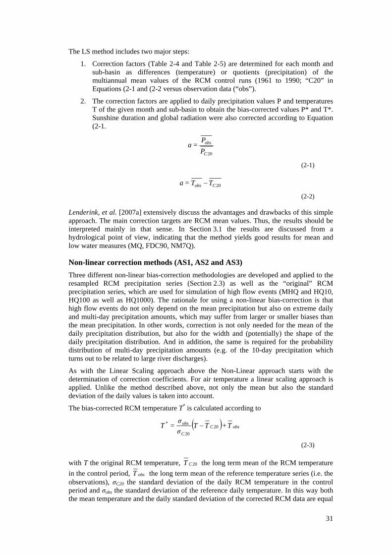
31
The LS method includes two major steps:
1. Correction factors (Table 2-4 and Table 2-5) are determined for each month and sub-basin as differences (temperature) or quotients (precipitation) of the multiannual mean values of the RCM control runs (1961 to 1990; “C20” in Equations (2-1 and (2-2 versus observation data (“obs”).
2. The correction factors are applied to daily precipitation values P and temperatures T of the given month and sub-basin to obtain the bias-corrected values P* and T*. Sunshine duration and global radiation were also corrected according to Equation (2-1.
20C
obs
PP
=a
(2-1)
20Cobs TT=a −
(2-2)
Lenderink, et al. [2007a] extensively discuss the advantages and drawbacks of this simple approach. The main correction targets are RCM mean values. Thus, the results should be interpreted mainly in that sense. In Section 3.1 the results are discussed from a hydrological point of view, indicating that the method yields good results for mean and low water measures (MQ, FDC90, NM7Q).
Non-linear correction methods (AS1, AS2 and AS3) Three different non-linear bias-correction methodologies are developed and applied to the resampled RCM precipitation series (Section 2.3) as well as the “original” RCM precipitation series, which are used for simulation of high flow events (MHQ and HQ10, HQ100 as well as HQ1000). The rationale for using a non-linear bias-correction is that high flow events do not only depend on the mean precipitation but also on extreme daily and multi-day precipitation amounts, which may suffer from larger or smaller biases than the mean precipitation. In other words, correction is not only needed for the mean of the daily precipitation distribution, but also for the width and (potentially) the shape of the daily precipitation distribution. And in addition, the same is required for the probability distribution of multi-day precipitation amounts (e.g. of the 10-day precipitation which turns out to be related to large river discharges).
As with the Linear Scaling approach above the Non-Linear approach starts with the determination of correction coefficients. For air temperature a linear scaling approach is applied. Unlike the method described above, not only the mean but also the standard deviation of the daily values is taken into account.
The bias-corrected RCM temperature T* is calculated according to
( ) obsCC
obs T+TTσσ
=T 2020
* −
(2-3)
with T the original RCM temperature, 20CT the long term mean of the RCM temperature in the control period, obsT the long term mean of the reference temperature series (i.e. the observations), σC20 the standard deviation of the daily RCM temperature in the control period and σobs the standard deviation of the reference daily temperature. In this way both the mean temperature and the daily standard deviation of the corrected RCM data are equal
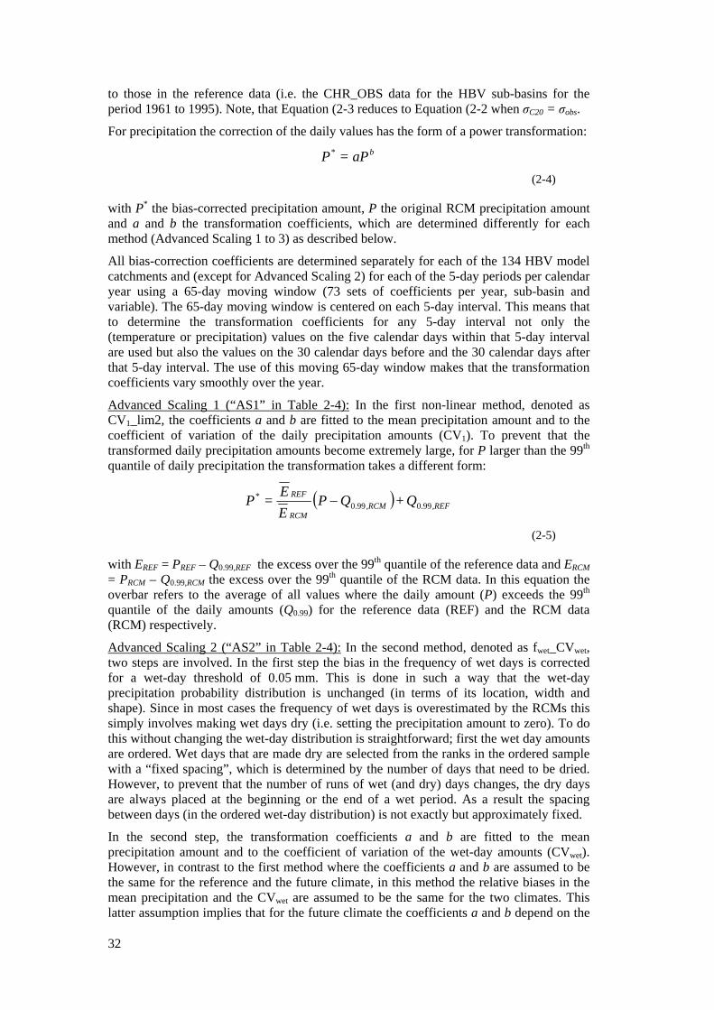
32
to those in the reference data (i.e. the CHR_OBS data for the HBV sub-basins for the period 1961 to 1995). Note, that Equation (2-3 reduces to Equation (2-2 when σC20 = σobs.
For precipitation the correction of the daily values has the form of a power transformation: baP=P*
(2-4)
with P* the bias-corrected precipitation amount, P the original RCM precipitation amount and a and b the transformation coefficients, which are determined differently for each method (Advanced Scaling 1 to 3) as described below.
All bias-correction coefficients are determined separately for each of the 134 HBV model catchments and (except for Advanced Scaling 2) for each of the 5-day periods per calendar year using a 65-day moving window (73 sets of coefficients per year, sub-basin and variable). The 65-day moving window is centered on each 5-day interval. This means that to determine the transformation coefficients for any 5-day interval not only the (temperature or precipitation) values on the five calendar days within that 5-day interval are used but also the values on the 30 calendar days before and the 30 calendar days after that 5-day interval. The use of this moving 65-day window makes that the transformation coefficients vary smoothly over the year.
Advanced Scaling 1 (“AS1” in Table 2-4): In the first non-linear method, denoted as CV1_lim2, the coefficients a and b are fitted to the mean precipitation amount and to the coefficient of variation of the daily precipitation amounts (CV1). To prevent that the transformed daily precipitation amounts become extremely large, for P larger than the 99th quantile of daily precipitation the transformation takes a different form:
( ) REF,RCM,RCM
REF Q+QPEE=P 0.990.99
* −
(2-5)
with EREF = PREF – Q0.99,REF the excess over the 99th quantile of the reference data and ERCM = PRCM – Q0.99,RCM the excess over the 99th quantile of the RCM data. In this equation the overbar refers to the average of all values where the daily amount (P) exceeds the 99th quantile of the daily amounts (Q0.99) for the reference data (REF) and the RCM data (RCM) respectively.
Advanced Scaling 2 (“AS2” in Table 2-4): In the second method, denoted as fwet_CVwet, two steps are involved. In the first step the bias in the frequency of wet days is corrected for a wet-day threshold of 0.05 mm. This is done in such a way that the wet-day precipitation probability distribution is unchanged (in terms of its location, width and shape). Since in most cases the frequency of wet days is overestimated by the RCMs this simply involves making wet days dry (i.e. setting the precipitation amount to zero). To do this without changing the wet-day distribution is straightforward; first the wet day amounts are ordered. Wet days that are made dry are selected from the ranks in the ordered sample with a “fixed spacing”, which is determined by the number of days that need to be dried. However, to prevent that the number of runs of wet (and dry) days changes, the dry days are always placed at the beginning or the end of a wet period. As a result the spacing between days (in the ordered wet-day distribution) is not exactly but approximately fixed.
In the second step, the transformation coefficients a and b are fitted to the mean precipitation amount and to the coefficient of variation of the wet-day amounts (CVwet). However, in contrast to the first method where the coefficients a and b are assumed to be the same for the reference and the future climate, in this method the relative biases in the mean precipitation and the CVwet are assumed to be the same for the two climates. This latter assumption implies that for the future climate the coefficients a and b depend on the
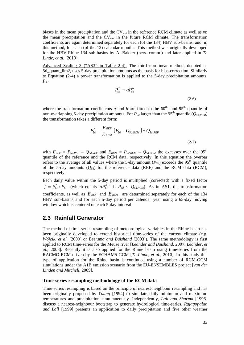
33
biases in the mean precipitation and the CVwet in the reference RCM climate as well as on the mean precipitation and the CVwet in the future RCM climate. The transformation coefficients are again determined separately for each (of the 134) HBV sub-basins, and, in this method, for each (of the 12) calendar months. This method was originally developed for the HBV-Rhine 134 sub-basins by A. Bakker (pers. comm.) and later applied in Te Linde, et al. [2010].
Advanced Scaling 3 (“AS3” in Table 2-4): The third non-linear method, denoted as 5d_quant_lim2, uses 5-day precipitation amounts as the basis for bias-correction. Similarly to Equation (2-4) a power transformation is applied to the 5-day precipitation amounts, P5d:
b5daP=P*
5d
(2-6)
where the transformation coefficients a and b are fitted to the 60th- and 95th quantile of non-overlapping 5-day precipitation amounts. For P5d larger than the 95th quantile (Q5d,RCM) the transformation takes a different form:
( ) REF,RCM,RCM
REF Q+QPEE=P 5d5d5d
*5d −
(2-7)
with EREF = P5d,REF – Q5d,REF and ERCM = P5d,RCM – Q5d,RCM the excesses over the 95th quantile of the reference and the RCM data, respectively. In this equation the overbar refers to the average of all values where the 5-day amount (P5d) exceeds the 95th quantile of the 5-day amounts (Q5d) for the reference data (REF) and the RCM data (RCM), respectively.
Each daily value within the 5-day period is multiplied (corrected) with a fixed factor
5d*
5d / PPf = (which equals 1−b5daP if P5d < Q5d,RCM). As in AS1, the transformation
coefficients, as well as REFE and RCME , are determined separately for each of the 134 HBV sub-basins and for each 5-day period per calendar year using a 65-day moving window which is centered on each 5-day interval.
2.3 Rainfall Generator
The method of time-series resampling of meteorological variables in the Rhine basin has been originally developed to extend historical time-series of the current climate (e.g. Wójcik, et al. [2000] or Beersma and Buishand [2003]). The same methodology is first applied to RCM time-series for the Meuse river [Leander and Buishand, 2007; Leander, et al., 2008]. Recently it is also applied for the Rhine basin using time-series from the RACMO RCM driven by the ECHAM5 GCM [Te Linde, et al., 2010]. In this study this type of application for the Rhine basin is continued using a number of RCM-GCM simulations under the A1B emission scenario from the EU-ENSEMBLES project [van der Linden and Mitchell, 2009].
Time-series resampling methodology of the RCM data Time-series resampling is based on the principle of nearest-neighbour resampling and has been originally proposed by Young [1994] to simulate daily minimum and maximum temperatures and precipitation simultaneously. Independently, Lall and Sharma [1996] discuss a nearest-neighbour bootstrap to generate hydrological time-series. Rajagopalan and Lall [1999] presents an application to daily precipitation and five other weather
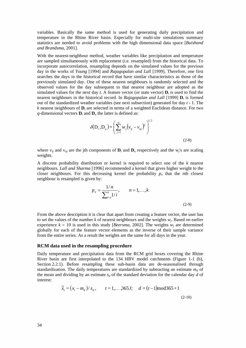
34
variables. Basically the same method is used for generating daily precipitation and temperature in the Rhine River basin. Especially for multi-site simulations summary statistics are needed to avoid problems with the high dimensional data space [Buishand and Brandsma, 2001].
With the nearest-neighbour method, weather variables like precipitation and temperature are sampled simultaneously with replacement (i.e. resampled) from the historical data. To incorporate autocorrelation, resampling depends on the simulated values for the previous day in the works of Young [1994] and Rajagopalan and Lall [1999]. Therefore, one first searches the days in the historical record that have similar characteristics as those of the previously simulated day. One of these nearest neighbours is randomly selected and the observed values for the day subsequent to that nearest neighbour are adopted as the simulated values for the next day t. A feature vector (or state vector) Dt is used to find the nearest neighbours in the historical record. In Rajagopalan and Lall [1999] Dt is formed out of the standardized weather variables (see next subsection) generated for day t - 1. The k nearest neighbours of Dt are selected in terms of a weighted Euclidean distance. For two q-dimensional vectors Dt and Du the latter is defined as:
( ) ( )2/1
1
2DD ⎟⎟⎠
⎞⎜⎜⎝
⎛−∑
q
j=ujtjjut vvw=,δ
(2-8)
where vtj and vuj are the jth components of Dt and Du respectively and the wj's are scaling weights.
A discrete probability distribution or kernel is required to select one of the k nearest neighbours. Lall and Sharma [1996] recommended a kernel that gives higher weight to the closer neighbours. For this decreasing kernel the probability pn that the nth closest neighbour is resampled is given by:
kni
np k
i
n ,,1 ,/1
/1
1
K==∑ =
(2-9)
From the above description it is clear that apart from creating a feature vector, the user has to set the values of the number k of nearest neighbours and the weights wj. Based on earlier experience k = 10 is used in this study [Beersma, 2002]. The weights wj are determined globally for each of the feature vector elements as the inverse of their sample variance from the entire series. As a result the weights are the same for all days in the year.
RCM data used in the resampling procedure Daily temperature and precipitation data from the RCM grid boxes covering the Rhine River basin are first interpolated to the 134 HBV model catchments (Figure 1-1 (b), Section 2.2.1). Before resampling these sub-basin data are de-seasonalised through standardization. The daily temperatures are standardized by subtracting an estimate md of the mean and dividing by an estimate sd of the standard deviation for the calendar day d of interest:
( ) ( ) 1mod3651 3651, /~ +t=dJ;,=t,smx=x ddtt −…−
(2-10)
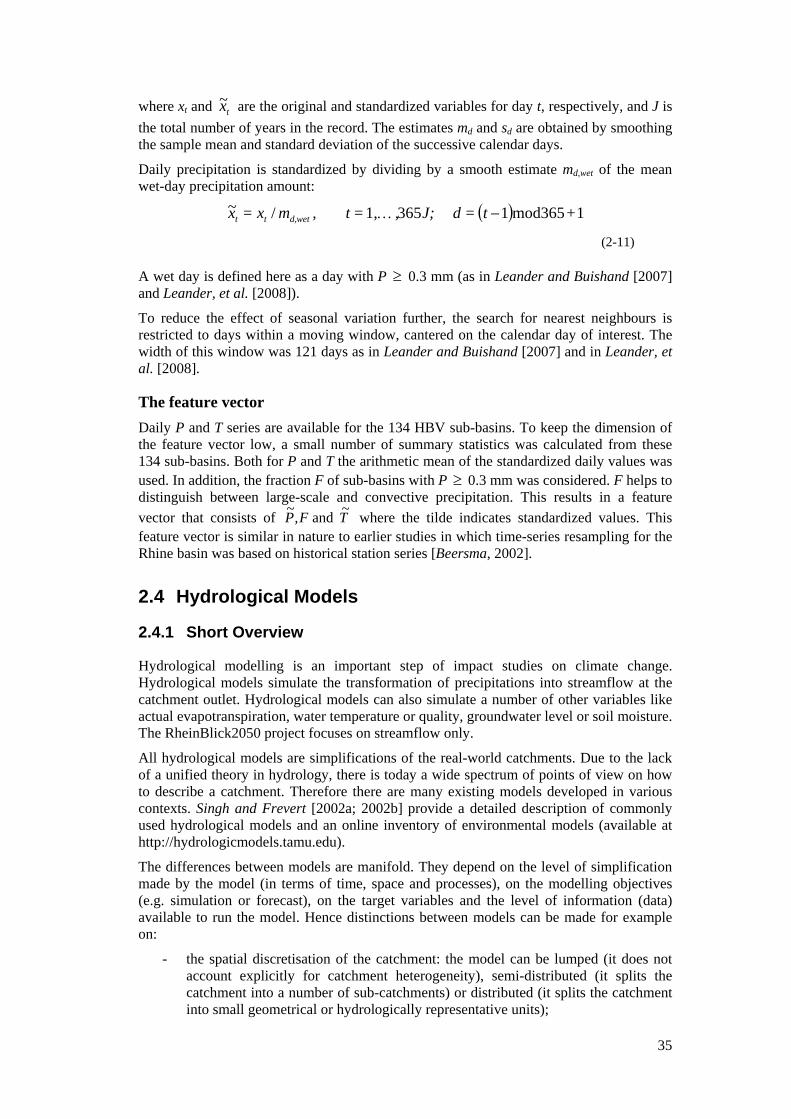
35
where xt and tx~ are the original and standardized variables for day t, respectively, and J is the total number of years in the record. The estimates md and sd are obtained by smoothing the sample mean and standard deviation of the successive calendar days.
Daily precipitation is standardized by dividing by a smooth estimate md,wet of the mean wet-day precipitation amount:
( ) 1mod3651 3651, /~ +t=dJ;,=t,mx=x wetd,tt −…
(2-11)
A wet day is defined here as a day with P ≥ 0.3 mm (as in Leander and Buishand [2007] and Leander, et al. [2008]).
To reduce the effect of seasonal variation further, the search for nearest neighbours is restricted to days within a moving window, cantered on the calendar day of interest. The width of this window was 121 days as in Leander and Buishand [2007] and in Leander, et al. [2008].
The feature vector Daily P and T series are available for the 134 HBV sub-basins. To keep the dimension of the feature vector low, a small number of summary statistics was calculated from these 134 sub-basins. Both for P and T the arithmetic mean of the standardized daily values was used. In addition, the fraction F of sub-basins with P ≥ 0.3 mm was considered. F helps to distinguish between large-scale and convective precipitation. This results in a feature vector that consists of TF,P ~ and ~ where the tilde indicates standardized values. This feature vector is similar in nature to earlier studies in which time-series resampling for the Rhine basin was based on historical station series [Beersma, 2002].
2.4 Hydrological Models
2.4.1 Short Overview
Hydrological modelling is an important step of impact studies on climate change. Hydrological models simulate the transformation of precipitations into streamflow at the catchment outlet. Hydrological models can also simulate a number of other variables like actual evapotranspiration, water temperature or quality, groundwater level or soil moisture. The RheinBlick2050 project focuses on streamflow only.
All hydrological models are simplifications of the real-world catchments. Due to the lack of a unified theory in hydrology, there is today a wide spectrum of points of view on how to describe a catchment. Therefore there are many existing models developed in various contexts. Singh and Frevert [2002a; 2002b] provide a detailed description of commonly used hydrological models and an online inventory of environmental models (available at http://hydrologicmodels.tamu.edu).
The differences between models are manifold. They depend on the level of simplification made by the model (in terms of time, space and processes), on the modelling objectives (e.g. simulation or forecast), on the target variables and the level of information (data) available to run the model. Hence distinctions between models can be made for example on:
- the spatial discretisation of the catchment: the model can be lumped (it does not account explicitly for catchment heterogeneity), semi-distributed (it splits the catchment into a number of sub-catchments) or distributed (it splits the catchment into small geometrical or hydrologically representative units);
36
- the temporal resolution, i.e. the model running time-step (annual water balance models are generally simpler than hourly models) or the way past conditions are accounted for (e.g. event-based versus continuous models);
- the level of process description: the model structure may include no explicit hydrological process (e.g. artificial neural network), be based on the mathematical implementation of physical laws (physically-based models), or use simplified process representations (conceptual or empirical models).
The list of possible differences between models could be continued, but this is out of the scope of this report. One can simply note that these differences between models will generate differences in their outputs. This is true under current conditions, as shown by many existing comparative studies of hydrological models (see e.g. Perrin, et al. [2001]; Smith, et al. [2004]). This is also true under future climate conditions as shown by studies investigating the impacts of possible climate change. Therefore the conclusions of these studies may partly depend on the selected model(s). For example, Jiang, et al. [2007] notice that significant differences can be obtained when running six different monthly models in China with the same climate change scenarios.
To account for this possible source of uncertainty, a selection of hydrological models is made in the RheinBlick2050 project. Two types of models are used:
- a semi-distributed conceptual model, called HBV [Bergström, 1995], adapted to the case of the Rhine basin;
- a few lumped conceptual models, not specifically tested on the Rhine basin but widely used in hydrological studies.
All these models are continuous and run at a daily time-step. They are driven by similar data (daily series of rainfall and temperature, evaporation). The main differences between the semi-distributed HBV model and the lumped models lie in the catchment spatial discretisation and in the level of process description. The following sections provide a short description of the models used. More detailed information on the model structures is given in Appendix C.
2.4.2 Semi-Distributed Model HBV
The HBV model is a semi-distributed conceptual hydrological model for continuous calculation of runoff which has been originally developed at the Swedish Meteorological and Hydrological Institute (SMHI) in the 1970s [Bergström, 1976; Bergström and Forsman, 1973]. In the 1990s major changes in the model structure have been made as published by Lindström, et al. [1997].
The main components of HBV are routines for snow accumulation and melt, a soil moisture accounting procedure, routines for runoff generation and a simple routing method. The spatial discretisation is defined by sub-basins which can be further divided into zones of different elevation and land cover (forest, non forest, lake and glacier).
Meanwhile manifold operational or scientific applications of HBV exist which are reported from more than 50 countries around the world. The model serves e.g. in the field of forecasting or climate impact modelling. In detail, the model structure of HBV is described in Appendix C.
The advantage of HBV is that it can be setup with a relative low number of parameters, it gives a good performance and can be handled easily, which is important, when modelling a big catchment such as the Rhine River basin. As with any model there are also limitations. These are described and quantified in detail using an inter-model comparison (Section 3.3.1). An evaluation of some limitations in the specific context of this study is given in Section 3.4.
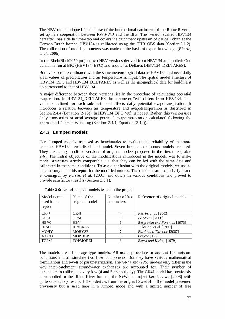
37
The HBV model adopted for the case of the international catchment of the Rhine River is set up in a cooperation between RWS-WD and the BfG. This version (called HBV134 hereafter) has a daily time-step and covers the catchment upstream of gauge Lobith at the German-Dutch border. HBV134 is calibrated using the CHR_OBS data (Section 2.1.2). The calibration of model parameters was made on the basis of expert knowledge [Eberle, et al., 2005].
In the RheinBlick2050 project two HBV versions derived from HBV134 are applied: One version is run at BfG (HBV134_BFG) and another at Deltares (HBV134_DELTARES).
Both versions are calibrated with the same meteorological data as HBV134 and need daily areal values of precipitation and air temperature as input. The spatial model structure of HBV134_BFG and HBV134_DELTARES as well as the geographical data for building it up correspond to that of HBV134.
A major difference between these versions lies in the procedure of calculating potential evaporation. In HBV134_DELTARES the parameter “etf” differs from HBV134. This value is defined for each sub-basin and affects daily potential evapotranspiration. It introduces a relation between air temperature and evapotranspiration as described in Section 2.4.4 (Equation (2-13)). In HBV134_BFG “etf” is not set. Rather, this version uses daily time-series of areal average potential evapotranspiration calculated following the approach of Penman Wendling (Section 2.4.4, Equation (2-12)).
2.4.3 Lumped models
Here lumped models are used as benchmarks to evaluate the reliability of the more complex HBV134 semi-distributed model. Seven lumped continuous models are used. They are mainly modified versions of original models proposed in the literature (Table 2-6). The initial objective of the modifications introduced in the models was to make model structures strictly comparable, i.e. that they can be fed with the same data and calibrated in the same conditions. To avoid confusion with the original models, we use 4-letter acronyms in this report for the modified models. These models are extensively tested at Cemagref by Perrin, et al. [2001] and others in various conditions and proved to provide satisfactory results (Section 3.3.1).
Table 2-6: List of lumped models tested in the project.
Model name used in the report
Name of the original model
Number of free parameters
Reference of original models
GR4J GR4J 4 Perrin, et al. [2003] GR5J GR5J 5 Le Moine [2008] HBV0 HBV 9 Bergström and Forsman [1973] IHAC IHACRES 6 Jakeman, et al. [1990] MOHY MOHYSE 7 Fortin and Turcotte [2007] MORD MORDOR 6 Garçon [1996] TOPM TOPMODEL 8 Beven and Kirkby [1979]
The models are all storage type models. All use a procedure to account for moisture conditions and all simulate two flow components. But they have various mathematical formulations and levels of parameterization. The GR4J and GR5J models only differ in the way inter-catchment groundwater exchanges are accounted for. Their number of parameters to calibrate is very low (4 and 5 respectively). The GR4J model has previously been applied to the Rhine River basin in the NeWater project Lerat, et al. [2006] with quite satisfactory results. HBV0 derives from the original Swedish HBV model presented previously but is used here in a lumped mode and with a limited number of free
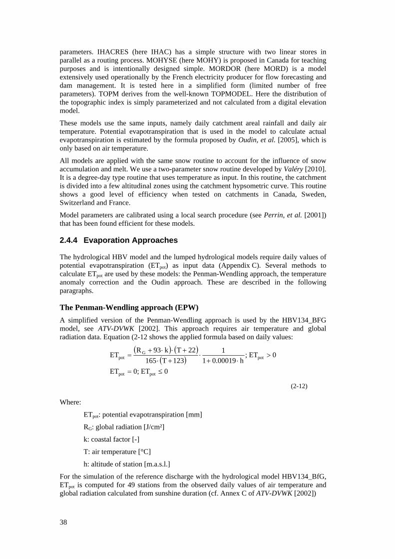
38
parameters. IHACRES (here IHAC) has a simple structure with two linear stores in parallel as a routing process. MOHYSE (here MOHY) is proposed in Canada for teaching purposes and is intentionally designed simple. MORDOR (here MORD) is a model extensively used operationally by the French electricity producer for flow forecasting and dam management. It is tested here in a simplified form (limited number of free parameters). TOPM derives from the well-known TOPMODEL. Here the distribution of the topographic index is simply parameterized and not calculated from a digital elevation model.
These models use the same inputs, namely daily catchment areal rainfall and daily air temperature. Potential evapotranspiration that is used in the model to calculate actual evapotranspiration is estimated by the formula proposed by Oudin, et al. [2005], which is only based on air temperature.
All models are applied with the same snow routine to account for the influence of snow accumulation and melt. We use a two-parameter snow routine developed by Valéry [2010]. It is a degree-day type routine that uses temperature as input. In this routine, the catchment is divided into a few altitudinal zones using the catchment hypsometric curve. This routine shows a good level of efficiency when tested on catchments in Canada, Sweden, Switzerland and France.
Model parameters are calibrated using a local search procedure (see Perrin, et al. [2001]) that has been found efficient for these models.
2.4.4 Evaporation Approaches
The hydrological HBV model and the lumped hydrological models require daily values of potential evapotranspiration (ETpot) as input data (Appendix C). Several methods to calculate ETpot are used by these models: the Penman-Wendling approach, the temperature anomaly correction and the Oudin approach. These are described in the following paragraphs.
The Penman-Wendling approach (EPW) A simplified version of the Penman-Wendling approach is used by the HBV134_BFG model, see ATV-DVWK [2002]. This approach requires air temperature and global radiation data. Equation (2-12 shows the applied formula based on daily values:
( ) ( )( )
0ET0;ET
0ET;h0.000191
1123T165
22Tk93RET
potpot
potG
pot
≤=
>⋅+
⋅+⋅
+⋅⋅+=
(2-12)
Where:
ETpot: potential evapotranspiration [mm]
RG: global radiation [J/cm²]
k: coastal factor [-]
T: air temperature [°C]
h: altitude of station [m.a.s.l.]
For the simulation of the reference discharge with the hydrological model HBV134_BfG, ETpot is computed for 49 stations from the observed daily values of air temperature and global radiation calculated from sunshine duration (cf. Annex C of ATV-DVWK [2002])
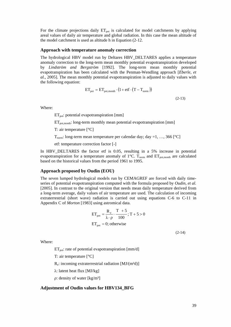
39
For the climate projections daily ETpot is calculated for model catchments by applying areal values of daily air temperature and global radiation. In this case the mean altitude of the model catchment is used as altitude h in Equation (2-12.
Approach with temperature anomaly correction The hydrological HBV model run by Deltares HBV_DELTARES applies a temperature anomaly correction to the long-term mean monthly potential evapotranspiration developed by Lindström and Bergström [1992]. The long-term mean monthly potential evapotranspiration has been calculated with the Penman-Wendling approach [Eberle, et al., 2005]. The mean monthly potential evapotranspiration is adjusted to daily values with the following equation:
( )( )normmonthpot,pot TTetf1ETET −⋅+⋅=
(2-13)
Where:
ETpot: potential evapotranspiration [mm]
ETpot,month: long-term monthly mean potential evapotranspiration [mm]
T: air temperature [°C]
Tnorm: long-term mean temperature per calendar day; day =1, …, 366 [°C]
etf: temperature correction factor [-]
In HBV_DELTARES the factor etf is 0.05, resulting in a 5% increase in potential evapotranspiration for a temperature anomaly of 1°C. Tnorm and ETpot,month are calculated based on the historical values from the period 1961 to 1995.
Approach proposed by Oudin (EOU) The seven lumped hydrological models run by CEMAGREF are forced with daily time-series of potential evapotranspiration computed with the formula proposed by Oudin, et al. [2005]. In contrast to the original version that needs mean daily temperature derived from a long-term average, daily values of air temperature are used. The calculation of incoming extraterrestrial (short wave) radiation is carried out using equations C-6 to C-11 in Appendix C of Morton [1983] using astromical data.
otherwise0;ET
05T;100
5Tρλ
RET
pot
epot
=
>++
⋅⋅
=
(2-14)
Where:
ETpot: rate of potential evapotranspiration [mm/d]
T: air temperature [°C]
Re: incoming extraterrestrial radiation [MJ/(m²d)]
λ: latent heat flux [MJ/kg]
ρ: density of water [kg/m³]
Adjustment of Oudin values for HBV134_BFG
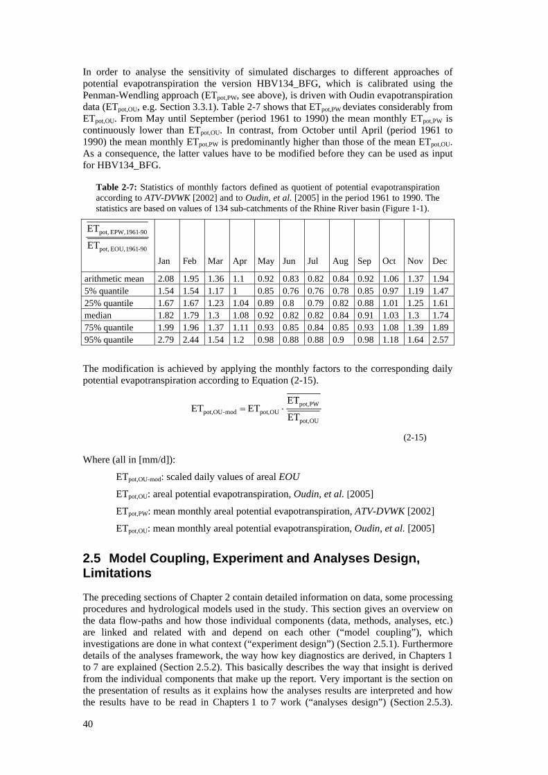
40
In order to analyse the sensitivity of simulated discharges to different approaches of potential evapotranspiration the version HBV134_BFG, which is calibrated using the Penman-Wendling approach (ETpot,PW, see above), is driven with Oudin evapotranspiration data (ETpot,OU, e.g. Section 3.3.1). Table 2-7 shows that ETpot,PW deviates considerably from ETpot,OU. From May until September (period 1961 to 1990) the mean monthly ETpot,PW is continuously lower than ETpot,OU. In contrast, from October until April (period 1961 to 1990) the mean monthly ETpot,PW is predominantly higher than those of the mean ETpot,OU. As a consequence, the latter values have to be modified before they can be used as input for HBV134_BFG.
Table 2-7: Statistics of monthly factors defined as quotient of potential evapotranspiration according to ATV-DVWK [2002] and to Oudin, et al. [2005] in the period 1961 to 1990. The statistics are based on values of 134 sub-catchments of the Rhine River basin (Figure 1-1).
ET
ET
90-1961 EOU, pot,
90-1961 EPW, pot,
Jan Feb Mar Apr May Jun Jul Aug Sep Oct Nov Dec
arithmetic mean 2.08 1.95 1.36 1.1 0.92 0.83 0.82 0.84 0.92 1.06 1.37 1.94 5% quantile 1.54 1.54 1.17 1 0.85 0.76 0.76 0.78 0.85 0.97 1.19 1.47 25% quantile 1.67 1.67 1.23 1.04 0.89 0.8 0.79 0.82 0.88 1.01 1.25 1.61 median 1.82 1.79 1.3 1.08 0.92 0.82 0.82 0.84 0.91 1.03 1.3 1.74 75% quantile 1.99 1.96 1.37 1.11 0.93 0.85 0.84 0.85 0.93 1.08 1.39 1.89 95% quantile 2.79 2.44 1.54 1.2 0.98 0.88 0.88 0.9 0.98 1.18 1.64 2.57
The modification is achieved by applying the monthly factors to the corresponding daily potential evapotranspiration according to Equation (2-15).
ET
ET ET ET
OUpot,
PWpot,OUpot,mod-OUpot, ⋅=
(2-15)
Where (all in [mm/d]):
ETpot,OU-mod: scaled daily values of areal EOU
ETpot,OU: areal potential evapotranspiration, Oudin, et al. [2005]
ETpot,PW: mean monthly areal potential evapotranspiration, ATV-DVWK [2002]
ETpot,OU: mean monthly areal potential evapotranspiration, Oudin, et al. [2005]
2.5 Model Coupling, Experiment and Analyses Design, Limitations
The preceding sections of Chapter 2 contain detailed information on data, some processing procedures and hydrological models used in the study. This section gives an overview on the data flow-paths and how those individual components (data, methods, analyses, etc.) are linked and related with and depend on each other (“model coupling”), which investigations are done in what context (“experiment design”) (Section 2.5.1). Furthermore details of the analyses framework, the way how key diagnostics are derived, in Chapters 1 to 7 are explained (Section 2.5.2). This basically describes the way that insight is derived from the individual components that make up the report. Very important is the section on the presentation of results as it explains how the analyses results are interpreted and how the results have to be read in Chapters 1 to 7 work (“analyses design”) (Section 2.5.3).
41
Finally, Section 2.5.4. lists restrictions and limitations of the report in one exhaustive summary in addition to specific discussions throughout the report.
2.5.1 Data Flowpath
A schematic overview on the data flowpath through the individual project components and also the report is given in Figure 1-6 with the inter-connecting arrows that indicate data being transferred through interfaces from one building block. In each one of those data flowpath components data is modified, processed or generated by various software tools and models. Figure 2-4 basically shows the same flowpath, albeit with different datasets (e.g. GCM and RCM model outputs) and methods (bias-correction schemes) explicitely named as used throughout the report. It is the specific combinations of models, model outputs and processing chain components which matters in that plot as the resulting regional climate change projections make up the ensemble which we use.
There are several data flowpaths or processing chains, which are linked with each other. The sequential and rather long primary processing chain is discussed below (Figure 2-4) and needed for the understanding of the overall experiment design. There are additional specific studies, like the effect of evapotranspiration approaches on hydrological model results, the performance of hydrological models or the validation study on the reproduction of observed target discharge diagnostics (not depicted in the overviews). These are linked at some point to the overall processing chain and do affect settings and selections therein. The expressions “data flowpath”, “model chain” or “processing chain” are used synonymously in this report. A model chain implies only the (off-line) coupling via the respective outputs of a GCM to an RCM to a hydrological model. Although Figure 2-4 shows the core setup, it ignores very much many intermediate necessary steps that are dealt with at some point in the report.
The individual steps of the data flowpath can be described as follows (see annotation in Figure 2-4 for an assignment):
(1) After the complete selection process is done, mainly GCMs driven by the SRES A1B are used in RheinBlick2050. The A1 family of scenarios reflects a future anthropogenic development that assumes an integrated world. It is characterised by (a) rapid economic growth, (b) a global population of 9 billion in 2050 with a gradual decline afterwards, (c) a quick spread of new and efficient technologies and (d) socio-economic and cultural convergence with worldwide interactions; A1B in addition means a balanced emphasis on all energy sources.
(2) The GHG emissions from (1) are major drivers of the GCM simulation results. GCM results are not extensively used themselves in the report, except for some uncertainty and bandwidth considerations in Section 2.1.3. However as they are driving the RCM simulations, they are implicitely contained therein and as they are a major source of uncertainty they are always mentioned in conjunction with the RCM.
(3) RCM simulation results are available at a 6-hourly or daily timestep in our case mainly via the CERA and ENSEMBLES data gateways. From the available 3-dimensional fields only near surface boundary layer fields are of importance for the hydrological modelling. Results from statistical downscaling are not displayed in Figure 2-4 as they are not used furtheron in the study.
(4) With the retrieval or update of local RCM output repositories the data flowpath within the project starts. We automatically retrieve daily fields of near surface air temperature, total precipitation and global radiation or sunshine duration (Section 2.1.3). In order to use these extensive datasets efficiently they are restructured to uniform datasets (meta-data homogenisation, data formats, spatial domain and grid, temporal resolution, temporal coverage, adjusted calendar format, unit conversions, etc.) (Section 2.2 gives some insight). In a second step the regularly gridded model fields are spatially aggregated for
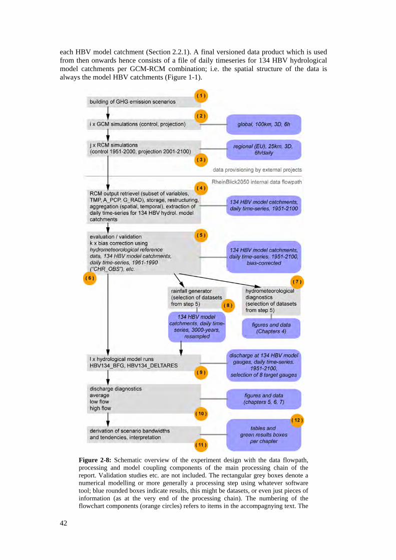
42
each HBV model catchment (Section 2.2.1). A final versioned data product which is used from then onwards hence consists of a file of daily timeseries for 134 HBV hydrological model catchments per GCM-RCM combination; i.e. the spatial structure of the data is always the model HBV catchments (Figure 1-1).
Figure 2-8: Schematic overview of the experiment design with the data flowpath, processing and model coupling components of the main processing chain of the report. Validation studies etc. are not included. The rectangular grey boxes denote a numerical modelling or more generally a processing step using whatever software tool; blue rounded boxes indicate results, this might be datasets, or even just pieces of information (as at the very end of the processing chain). The numbering of the flowchart components (orange circles) refers to items in the accompagnying text. The
43
indices (i, j, k, l) indicate that there are multiple combinations possible, see Figure 2-4.
(5) Chapter 3 deals very much with the validation and suitability of atmospheric forcing data and hydrological model results; to do this, many additional reference datasets are needed which are not listed here. Based on these studies, which form a fundamental part of the project, RCM model outputs are systematically evaluated whether they can be used for the hydrological impact study and also bias-corrected using different correction methods.
(6) For the aforementioned bias-correction a hydrometeorological reference dataset is needed. In RheinBlick2050 we use CHR_OBS (Section 2.1.2), which is also used to calibrate the HBV134 hydrological model.
(7) In order to investigate the meteorological changes in the Rhine River basin (Chapter 1) that eventually trigger the hydrological impacts, datasets from step 5 are sufficient. If no absolute value analyses were desired then even the bias-correction would even not be necessary.
(8) As it is statistically more reasonable to derive the discharge values for 100- and 1000-year return flows as part of the high flow investigations from a longer simulated discharge time-series (Section 7.1), a rainfall generator (Section 2.3) is used to re-sample 30-year timeslices of selected GCM-RCM-BC combinations to 3000-year daily timeseries, always based on the spatial structure of the 134 HBV model catchments.
(9) The hydrological model runs whose results are later on to be used in chapters 5 to 7 are hence driven by two atmospheric forcing datasets, 150 years and 3000 years. Two hydrological models HBV134_BFG and HBV134_DELTARES are run (Section 2.4.2).
(10) The discharge data analyses are based on the discharge simulation results from step 9. Target measures, i.e. specific average, high and low flow diagnostics, are derived for overall eight gauging stations (Section 2.5.2).
(11) From the relative changes of the target measures eventually the so-called scenario bandwidths and tendencies are derived for different time-slices, gauging stations and diagnostics (Section 2.5.3).
(12) The results from step 11 are the main findings in terms of climate change impacts on hydrology of the report. They are tabulated and summarised at the end of each analysis chapter.
2.5.2 Target Measures
As mentioned in Section 1.2 and as detailed in Appendix A, the target measures for assessing climate change impacts on discharge are negotiated with potential users of the report and stakeholders to ensure that data and analyses of the report – although no adaptation study is done – can easily be used and meet the respective requirements. So once the simulated daily discharge timeseries are available per gauging station at the very end of the modelling chain for past and future time-spans, specific discharge diagnostics are calculated depending on the purpose and subject of the investigation (average discharge, low or high flow). Here we give an overview on details of this analyses framework.
Selected gauges and spatial domain Discharge is analysed for six gauging stations along the Rhine River and for two at selected major tributaries (Table 2-8). Aside from the hydrometeorological investigations, all analyses are done for these gauging stations. The definition of these gauging stations is supposed to not only represent discharge conditions of the Rhine River itself but also those of the major tributaries, i.e. Neckar, Main, Moselle and Saar and the rivers in the Alpine
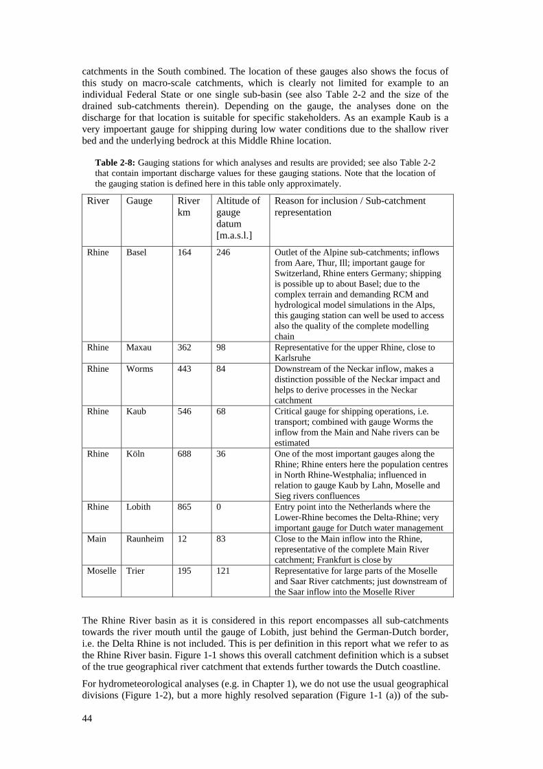
44
catchments in the South combined. The location of these gauges also shows the focus of this study on macro-scale catchments, which is clearly not limited for example to an individual Federal State or one single sub-basin (see also Table 2-2 and the size of the drained sub-catchments therein). Depending on the gauge, the analyses done on the discharge for that location is suitable for specific stakeholders. As an example Kaub is a very impoertant gauge for shipping during low water conditions due to the shallow river bed and the underlying bedrock at this Middle Rhine location.
Table 2-8: Gauging stations for which analyses and results are provided; see also Table 2-2 that contain important discharge values for these gauging stations. Note that the location of the gauging station is defined here in this table only approximately.
River Gauge River km
Altitude of gauge datum [m.a.s.l.]
Reason for inclusion / Sub-catchment representation
Rhine Basel 164 246 Outlet of the Alpine sub-catchments; inflows from Aare, Thur, Ill; important gauge for Switzerland, Rhine enters Germany; shipping is possible up to about Basel; due to the complex terrain and demanding RCM and hydrological model simulations in the Alps, this gauging station can well be used to access also the quality of the complete modelling chain
Rhine Maxau 362 98 Representative for the upper Rhine, close to Karlsruhe
Rhine Worms 443 84 Downstream of the Neckar inflow, makes a distinction possible of the Neckar impact and helps to derive processes in the Neckar catchment
Rhine Kaub 546 68 Critical gauge for shipping operations, i.e. transport; combined with gauge Worms the inflow from the Main and Nahe rivers can be estimated
Rhine Köln 688 36 One of the most important gauges along the Rhine; Rhine enters here the population centres in North Rhine-Westphalia; influenced in relation to gauge Kaub by Lahn, Moselle and Sieg rivers confluences
Rhine Lobith 865 0 Entry point into the Netherlands where the Lower-Rhine becomes the Delta-Rhine; very important gauge for Dutch water management
Main Raunheim 12 83 Close to the Main inflow into the Rhine, representative of the complete Main River catchment; Frankfurt is close by
Moselle Trier 195 121 Representative for large parts of the Moselle and Saar River catchments; just downstream of the Saar inflow into the Moselle River
The Rhine River basin as it is considered in this report encompasses all sub-catchments towards the river mouth until the gauge of Lobith, just behind the German-Dutch border, i.e. the Delta Rhine is not included. This is per definition in this report what we refer to as the Rhine River basin. Figure 1-1 shows this overall catchment definition which is a subset of the true geographical river catchment that extends further towards the Dutch coastline.
For hydrometeorological analyses (e.g. in Chapter 1), we do not use the usual geographical divisions (Figure 1-2), but a more highly resolved separation (Figure 1-1 (a)) of the sub-
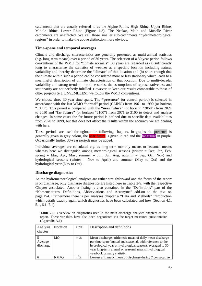
45
catchments that are usually referred to as the Alpine Rhine, High Rhine, Upper Rhine, Middle Rhine, Lower Rhine (Figure 1-3). The Neckar, Main and Moselle River catchments are unaffected. We call those smaller sub-catchments “hydrometeorological regions” in order to make the above distinction more obvious.
Time-spans and temporal averages Climate and discharge characteristics are generally presented as multi-annual statistics (e.g. long-term means) over a period of 30 years. The selection of a 30 year period follows conventions of the WMO for “climate normals”. 30 years are regarded as (a) sufficiently long to characterise the statistics of weather at a specific location including natural variability and thereby determine the “climate” of that location and (b) short enough that the climate within such a period can be considered more or less stationary which leads to a meaningful description of climate characteristics of that location. Due to multi-decadal variability and strong trends in the time-series, the assumptions of representativeness and stationarity are not perfectly fulfilled. However, to keep our results comparable to those of other projects (e.g. ENSEMBLES), we follow the WMO conventions.
We choose three 30-year time-spans. The “presence” (or control period) is selected in accordance with the last WMO “normal” period (CLINO) from 1961 to 1990 (or horizon “1990”). This period is compared with the “near future” (or horizon “2050”) from 2021 to 2050 and “far future” (or horizon “2100”) from 2071 to 2100 to detect and analyse changes. In some cases the far future period is defined due to specific data availabilities from 2070 to 2099, but this does not affect the results within the accuracy we are dealing with here.
These periods are used throughout the following chapters. In graphs the presence is generally given in grey colour, the near future is given in red and the far future in purple. Occasionally further 30-year periods may be added.
Individual averages are calculated e.g. as long-term monthly means or seasonal means whereas here we distinguish among meteorological seasons (winter = Dec, Jan, Feb; spring = Mar, Apr, May; summer = Jun, Jul, Aug; autumn = Sep, Oct, Nov) and hydrological seasons (winter = Nov to April) and summer (May to Oct) and the hydrological year (Nov to Oct).
Discharge diagnostics As the hydrometeorological analyses are rather straighforward and the focus of the report is on discharge, only discharge diagnostics are listed here in Table 2-9, with the respective Chapter associated. Another listing is also contained in the “Definitions” part of the “Nomenclatures, Definitions, Abbreviations and Acronyms” add-on to the text on page 154. Furthermore there is per analyses chapter a “Data and Methods” introduction which details exactly again which diagnostics have been calculated and how (Section 4.1, 5.1, 6.1, 7.1).
Table 2-9: Overview on diagnostics used in the main discharge analyses chapters of the report. These variables have also been degaotiated via the target measures questionnaire (Appendix A.1).
Analysis chapter
Notation Unit Description and definitions
5 Average discharge
MQ m3/s Mean discharge; arithmetic mean of daily mean discharge per time-span (annual and seasonal, with reference to the hydrological year or hydrological season); averaged to 30-year long-term annual or seasonal means; hydrological yearbook primary statistic
6 NM7Q m3/s Lowest arithmetic mean of discharge during 7 consecutive
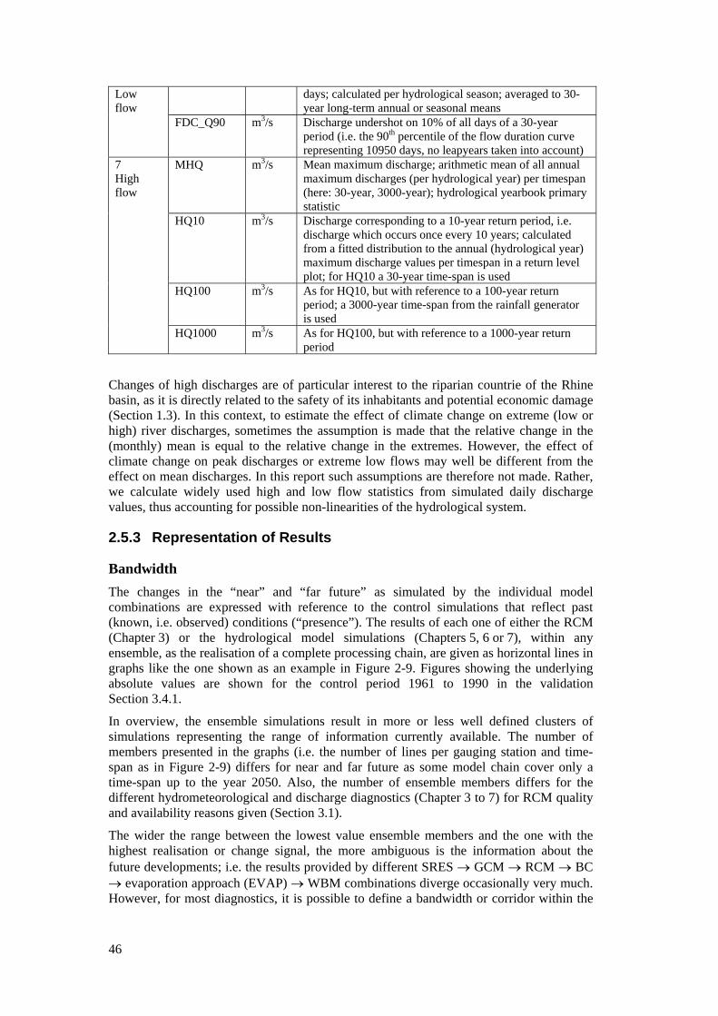
46
Low flow
days; calculated per hydrological season; averaged to 30-year long-term annual or seasonal means
FDC_Q90 m3/s Discharge undershot on 10% of all days of a 30-year period (i.e. the 90th percentile of the flow duration curve representing 10950 days, no leapyears taken into account)
7 High flow
MHQ m3/s Mean maximum discharge; arithmetic mean of all annual maximum discharges (per hydrological year) per timespan (here: 30-year, 3000-year); hydrological yearbook primary statistic
HQ10 m3/s Discharge corresponding to a 10-year return period, i.e. discharge which occurs once every 10 years; calculated from a fitted distribution to the annual (hydrological year) maximum discharge values per timespan in a return level plot; for HQ10 a 30-year time-span is used
HQ100 m3/s As for HQ10, but with reference to a 100-year return period; a 3000-year time-span from the rainfall generator is used
HQ1000 m3/s As for HQ100, but with reference to a 1000-year return period
Changes of high discharges are of particular interest to the riparian countrie of the Rhine basin, as it is directly related to the safety of its inhabitants and potential economic damage (Section 1.3). In this context, to estimate the effect of climate change on extreme (low or high) river discharges, sometimes the assumption is made that the relative change in the (monthly) mean is equal to the relative change in the extremes. However, the effect of climate change on peak discharges or extreme low flows may well be different from the effect on mean discharges. In this report such assumptions are therefore not made. Rather, we calculate widely used high and low flow statistics from simulated daily discharge values, thus accounting for possible non-linearities of the hydrological system.
2.5.3 Representation of Results
Bandwidth The changes in the “near” and “far future” as simulated by the individual model combinations are expressed with reference to the control simulations that reflect past (known, i.e. observed) conditions (“presence”). The results of each one of either the RCM (Chapter 3) or the hydrological model simulations (Chapters 5, 6 or 7), within any ensemble, as the realisation of a complete processing chain, are given as horizontal lines in graphs like the one shown as an example in Figure 2-9. Figures showing the underlying absolute values are shown for the control period 1961 to 1990 in the validation Section 3.4.1.
In overview, the ensemble simulations result in more or less well defined clusters of simulations representing the range of information currently available. The number of members presented in the graphs (i.e. the number of lines per gauging station and time-span as in Figure 2-9) differs for near and far future as some model chain cover only a time-span up to the year 2050. Also, the number of ensemble members differs for the different hydrometeorological and discharge diagnostics (Chapter 3 to 7) for RCM quality and availability reasons given (Section 3.1).
The wider the range between the lowest value ensemble members and the one with the highest realisation or change signal, the more ambiguous is the information about the future developments; i.e. the results provided by different SRES → GCM → RCM → BC → evaporation approach (EVAP) → WBM combinations diverge occasionally very much. However, for most diagnostics, it is possible to define a bandwidth or corridor within the
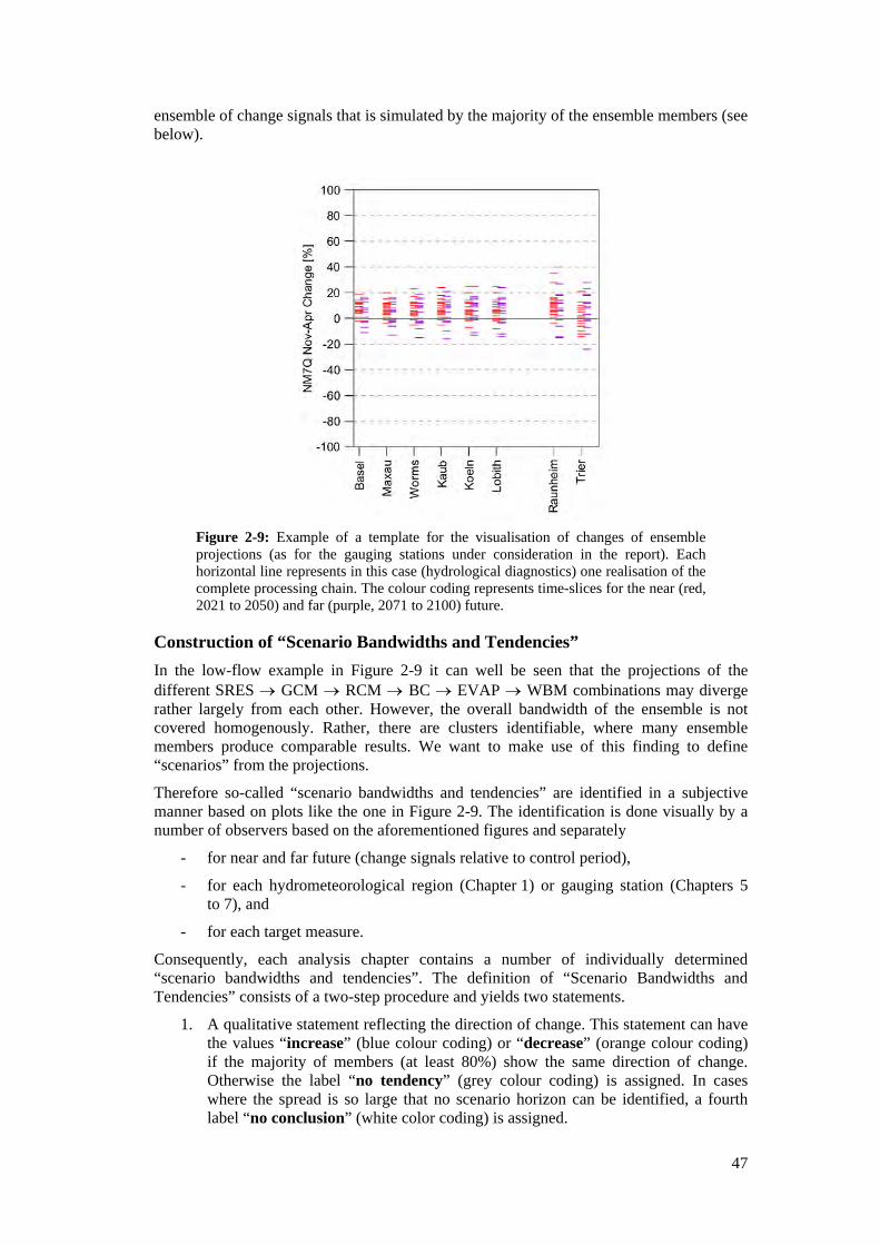
47
ensemble of change signals that is simulated by the majority of the ensemble members (see below).
Figure 2-9: Example of a template for the visualisation of changes of ensemble projections (as for the gauging stations under consideration in the report). Each horizontal line represents in this case (hydrological diagnostics) one realisation of the complete processing chain. The colour coding represents time-slices for the near (red, 2021 to 2050) and far (purple, 2071 to 2100) future.
Construction of “Scenario Bandwidths and Tendencies” In the low-flow example in Figure 2-9 it can well be seen that the projections of the different SRES → GCM → RCM → BC → EVAP → WBM combinations may diverge rather largely from each other. However, the overall bandwidth of the ensemble is not covered homogenously. Rather, there are clusters identifiable, where many ensemble members produce comparable results. We want to make use of this finding to define “scenarios” from the projections.
Therefore so-called “scenario bandwidths and tendencies” are identified in a subjective manner based on plots like the one in Figure 2-9. The identification is done visually by a number of observers based on the aforementioned figures and separately
- for near and far future (change signals relative to control period),
- for each hydrometeorological region (Chapter 1) or gauging station (Chapters 5 to 7), and
- for each target measure.
Consequently, each analysis chapter contains a number of individually determined “scenario bandwidths and tendencies”. The definition of “Scenario Bandwidths and Tendencies” consists of a two-step procedure and yields two statements.
1. A qualitative statement reflecting the direction of change. This statement can have the values “increase” (blue colour coding) or “decrease” (orange colour coding) if the majority of members (at least 80%) show the same direction of change. Otherwise the label “no tendency” (grey colour coding) is assigned. In cases where the spread is so large that no scenario horizon can be identified, a fourth label “no conclusion” (white color coding) is assigned.
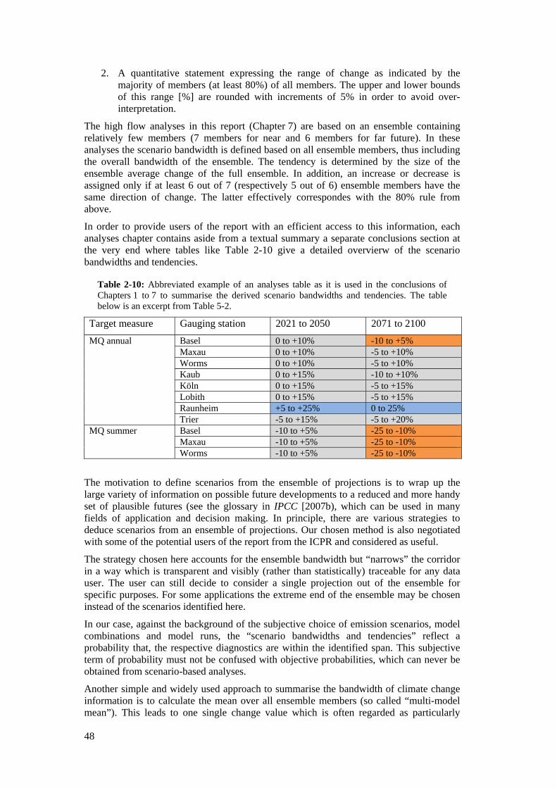
48
2. A quantitative statement expressing the range of change as indicated by the majority of members (at least 80%) of all members. The upper and lower bounds of this range [%] are rounded with increments of 5% in order to avoid over-interpretation.
The high flow analyses in this report (Chapter 7) are based on an ensemble containing relatively few members (7 members for near and 6 members for far future). In these analyses the scenario bandwidth is defined based on all ensemble members, thus including the overall bandwidth of the ensemble. The tendency is determined by the size of the ensemble average change of the full ensemble. In addition, an increase or decrease is assigned only if at least 6 out of 7 (respectively 5 out of 6) ensemble members have the same direction of change. The latter effectively correspondes with the 80% rule from above.
In order to provide users of the report with an efficient access to this information, each analyses chapter contains aside from a textual summary a separate conclusions section at the very end where tables like Table 2-10 give a detailed overvierw of the scenario bandwidths and tendencies.
Table 2-10: Abbreviated example of an analyses table as it is used in the conclusions of Chapters 1 to 7 to summarise the derived scenario bandwidths and tendencies. The table below is an excerpt from Table 5-2.
Target measure Gauging station 2021 to 2050 2071 to 2100
MQ annual Basel 0 to +10% -10 to +5% Maxau 0 to +10% -5 to +10% Worms 0 to +10% -5 to +10% Kaub 0 to +15% -10 to +10% Köln 0 to +15% -5 to +15% Lobith 0 to +15% -5 to +15% Raunheim +5 to +25% 0 to 25% Trier -5 to +15% -5 to +20%
MQ summer Basel -10 to +5% -25 to -10% Maxau -10 to +5% -25 to -10% Worms -10 to +5% -25 to -10%
The motivation to define scenarios from the ensemble of projections is to wrap up the large variety of information on possible future developments to a reduced and more handy set of plausible futures (see the glossary in IPCC [2007b), which can be used in many fields of application and decision making. In principle, there are various strategies to deduce scenarios from an ensemble of projections. Our chosen method is also negotiated with some of the potential users of the report from the ICPR and considered as useful.
The strategy chosen here accounts for the ensemble bandwidth but “narrows” the corridor in a way which is transparent and visibly (rather than statistically) traceable for any data user. The user can still decide to consider a single projection out of the ensemble for specific purposes. For some applications the extreme end of the ensemble may be chosen instead of the scenarios identified here.
In our case, against the background of the subjective choice of emission scenarios, model combinations and model runs, the “scenario bandwidths and tendencies” reflect a probability that, the respective diagnostics are within the identified span. This subjective term of probability must not be confused with objective probabilities, which can never be obtained from scenario-based analyses.
Another simple and widely used approach to summarise the bandwidth of climate change information is to calculate the mean over all ensemble members (so called “multi-model mean”). This leads to one single change value which is often regarded as particularly
49
useful by decision makers. However, there is no proof that multi-model means are more “likely” than the rest of the ensemble. Moreover, this simplistic approach makes it impossible to include the available range of information in planning processes. This could lead to wrong decisions on the necessity and dimension of adaptation measures.
2.5.4 Limitations of the Experiment Design The experiment design with its modelling and analysis framework as described above has many specific and known limitations. A detailed overview on specific restrictions and limitations of the data, methods and models is given where appropriate in Chapter 3. Here we give an overview of conceptual constraints.
Multi-Model RheinBlick2050 strictly follows a multi-model approach. We try to incorporate as many data resources as possible to be able to assess the uncertainty of the individual resources. The EU-ENSEMBLES project is the primary data source for the regional climate change projections. Here some model runs have become available during the duration of RheinBlick2050. Due to temporal and technical constraints those “late arrivals” could not be added to the already existing datasets.
Although an extensive model matrix with many emission scenarios, global and regional model combinations is developed, there is a clear domination of some elements (Section 2.1.3). The emission scenario A1B, and the globel climate models ECHAM5 and HadCM3 are incorporated more often that other SRES or GCMs; hence the results may be influenced by the characteristics of these models. We can not cover the real – albeit unknown – full bandwidth of the atmospheric and hydrologic physical system.
Model selection and weighting It is difficult to decide on a common set of quality criteria and benchmark tests in order to evaluate the suitability of regional climate model results. As can be shown in Chapter 3, the quality of individual models differs spatially, temporally and between different variables. Thus, we do not use a weighing of such results, but we select model chains based on simple, yet robust, plausibility checks (Section 3.1).
Elements of model chain RheinBlick2050 uses a complex model chain to assess the impact of changes in atmospheric GHG concentrations on Rhine River discharges. However, many simplifications are necessary to allow simulations for long periods (150 years), the large areas (Rhine River basin) and many model runs (SRES-GCM-RCM couplings). Thus, although the RheinBlick model chain includes many elements, it can not include all aspects relevant for discharges of the Rhine River. For example, models of land cover change or detailed hydrodynamic or morphodynamic models are missing. Also, feedbacks from possible future adaptation measures are not included.
Consequently, RheinBlick2050 produces results which are consistent within the specific model world. We give interpretations only for change signals between control and future periods as simulated by the individual model couplings. Comparisons of absolute discharge values between the “model world” and the “real world” are not always straight forward as (1) some effects (e.g. flooding, Section 3.4) are not fully covered in the model world (2) some effects may not be covered by the short observational timeseries.
Data analyses Not all discharge diagnostics requested by potential users (see questionnaire in Appendix A.1) could be dealt with in the analyses chapter of the report. However, we

50
select diagnostics which cover the full range of discharges from low flow to extreme high flow.
Due to the limited size (as compared to probabilistic ensembles) of the ensemble of the final hydrological model results, no descriptive statistics are calculated. Instead the ensembles of results are rounded off to obtain robust “scenario bandwidths and tendencies” (Section 2.5.3).
State of the art The results and analyses in the report are valid and consistent within the framework of the study. They are based on “state of the art” climate models, data and methods with a time-stamp of winter 2009/2010. Limitations and restrictions are mentioned here and throughout the text of the report where appropriate.
However, as emission scenarios change over time, global and regional climate models continuously improve, e.g. in the physical and bio-geo-chemical representation of relevant processes and spatial resolution, new methods for the treatment and analyses of large ensembles are developed, new and improved bias-correction methods become available and reference datasets improve continuously, similar studies should be conducted at regular intervals to account for substantial changes the “state of the art”.
Scale It is important to note that the study has a spatial focus on the complete Rhine River catchment. Data, modelling tools and methods have been chosen according to that spatial scale. The same data, modelling tools and methods may be unsuitable for other scales. Comparisons of results obtained on different spatial scales are not done in this report. They should, however, be an issue of future research.
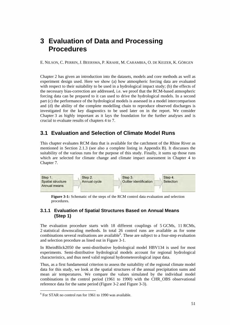
51
3 Evaluation of Data and Processing Procedures
E. NILSON, C. PERRIN, J. BEERSMA, P. KRAHE, M. CARAMBIA, O. DE KEIZER, K. GÖRGEN
Chapter 2 has given an introduction into the datasets, models and core methods as well as experiment design used. Here we show (a) how atmospheric forcing data are evaluated with respect to their suitability to be used in a hydrological impact study; (b) the effects of the necessary bias-correction are addressed, i.e. we proof that the RCM-based atmospheric forcing data can be prepared to it can used to drive the hydrological models. In a second part (c) the performance of the hydrological models is assessed in a model intercomparison and (d) the ability of the complete modelling chain to reproduce observed discharges is investigated for the key diagnostics to be used later on in the report. We consider Chapter 3 as highly important as it lays the foundation for the further analyses and is crucial to evaluate results of chapters 4 to 7.
3.1 Evaluation and Selection of Climate Model Runs
This chapter evaluates RCM data that is available for the catchment of the Rhine River as mentioned in Section 2.1.3 (see also a complete listing in Appendix B). It discusses the suitability of the various runs for the purpose of this study. Finally, it sums up those runs which are selected for climate change and climate impact assessment in Chapter 4 to Chapter 7.
Figure 3-1: Schematic of the steps of the RCM control data evaluation and selection procedures.
3.1.1 Evaluation of Spatial Structures Based on Annual Means (Step 1)
The evaluation procedure starts with 18 different couplings of 5 GCMs, 11 RCMs, 2 statistical downscaling methods. In total 26 control runs are available as for some combinations several realisations are available6. These are subject to a four-step evaluation and selection procedure as lined out in Figure 3-1.
In RheinBlick2050 the semi-distributive hydrological model HBV134 is used for most experiments. Semi-distributive hydrological models account for regional hydrological characteristics, and thus need valid regional hydrometeorological input data.
Thus, as a first fundamental criterion to assess the suitability of the regional climate model data for this study, we look at the spatial structures of the annual precipitation sums and mean air temperatures. We compare the values simulated by the individual model combinations in the control period (1961 to 1990) with the CHR_OBS observational reference data for the same period (Figure 3-2 and Figure 3-3). 6 For STAR no control run for 1961 to 1990 was available.
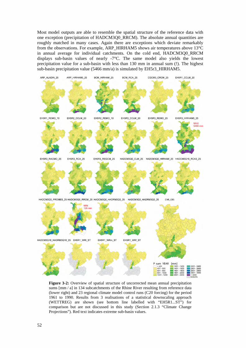
52
Most model outputs are able to resemble the spatial structure of the reference data with one exception (precipitation of HADCM3Q0_RRCM). The absolute annual quantities are roughly matched in many cases. Again there are exceptions which deviate remarkably from the observations. For example, ARP_HIRHAM5 shows air temperatures above 13°C in annual average for individual catchments. On the cold end, HADCM3Q0_RRCM displays sub-basin values of nearly -7°C. The same model also yields the lowest precipitation value for a sub-basin with less than 130 mm in annual sum (!). The highest sub-basin precipitation value (5466 mm/a) is simulated by EH5r3_HIRHAM5.
Figure 3-2: Overview of spatial structure of uncorrected mean annual precipitation sums [mm / a] in 134 subcatchments of the Rhine River resulting from reference data (lower right) and 23 regional climate model control runs (C20 forcing) for the period 1961 to 1990. Results from 3 realisations of a statistical downscaling approach (WETTREG) are shown (see bottom line labelled with “EH5R1...ST”) for comparison but are not discussed in this study (Section 2.1.3 “Climate Change Projections”). Red text indicates extreme sub-basin values.
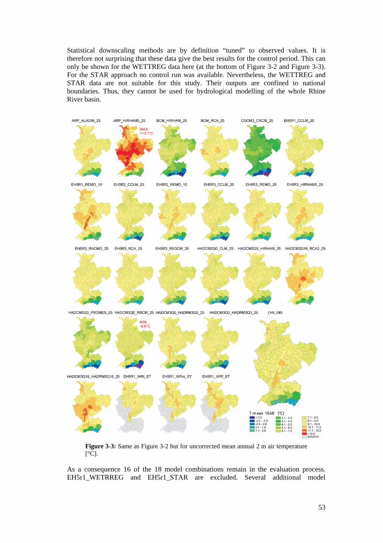
53
Statistical downscaling methods are by definition “tuned” to observed values. It is therefore not surprising that these data give the best results for the control period. This can only be shown for the WETTREG data here (at the bottom of Figure 3-2 and Figure 3-3). For the STAR approach no control run was available. Nevertheless, the WETTREG and STAR data are not suitable for this study. Their outputs are confined to national boundaries. Thus, they cannot be used for hydrological modelling of the whole Rhine River basin.
Figure 3-3: Same as Figure 3-2 but for uncorrected mean annual 2 m air temperature [°C].
As a consequence 16 of the 18 model combinations remain in the evaluation process. EH5r1_WETRREG and EH5r1_STAR are excluded. Several additional model
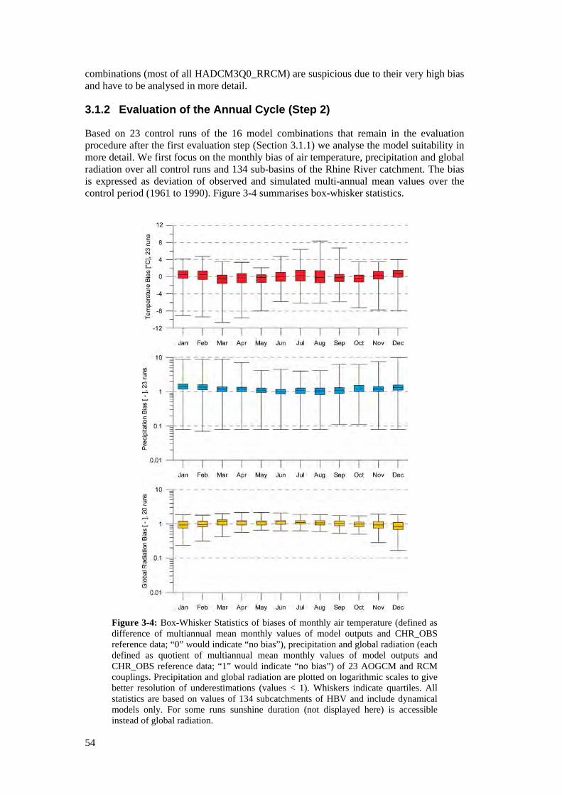
54
combinations (most of all HADCM3Q0_RRCM) are suspicious due to their very high bias and have to be analysed in more detail.
3.1.2 Evaluation of the Annual Cycle (Step 2)
Based on 23 control runs of the 16 model combinations that remain in the evaluation procedure after the first evaluation step (Section 3.1.1) we analyse the model suitability in more detail. We first focus on the monthly bias of air temperature, precipitation and global radiation over all control runs and 134 sub-basins of the Rhine River catchment. The bias is expressed as deviation of observed and simulated multi-annual mean values over the control period (1961 to 1990). Figure 3-4 summarises box-whisker statistics.
Figure 3-4: Box-Whisker Statistics of biases of monthly air temperature (defined as difference of multiannual mean monthly values of model outputs and CHR_OBS reference data; “0” would indicate “no bias”), precipitation and global radiation (each defined as quotient of multiannual mean monthly values of model outputs and CHR_OBS reference data; “1” would indicate “no bias”) of 23 AOGCM and RCM couplings. Precipitation and global radiation are plotted on logarithmic scales to give better resolution of underestimations (values < 1). Whiskers indicate quartiles. All statistics are based on values of 134 subcatchments of HBV and include dynamical models only. For some runs sunshine duration (not displayed here) is accessible instead of global radiation.
55
The median and 25./75. percentile range indicate, that the temperature bias lies within a moderate span of -1 to +1°C in most cases. Overestimates generally occur in winter (November, December, January, February), underestimates in the remaining months with the exception of July and August where the overall bias of the ensemble shows no clear direction. Precipitation biases are mainly positive, ranging from +10% to +50%, with larger overestimations in winter (January, February). Global radiation biases show a span from -25% to +10% with overestimations in most summer months (March to September).
The minimum/maximum range shows even more remarkable bias values. For example, mismatches between model outputs and observation data range from -10°C to +8°C for monthly air temperature and factors of 1/10 to 10 for monthly precipitation. Global radiation biases can be more than a factor of 2.
To sum up, model results match observed monthly mean values fairly well in many cases as shown by the narrow 25./75. percentile range of the bias. However, for individual model runs and subcatchments, bias values are extremely high. The overall bias could be largely reduced by eliminating these outliers.
3.1.3 Outlier Identification (Step 3)
The outliers are identified based on Figure 3-5 which gives a graphical overview of the seasonal (quarterly) temperature and precipitation bias for the 134 sub-basins of the Rhine River basin. The values are expressed with reference to the CHR_OBS values for the control period (1961 to 1990). Each cloud of symbols identifies one of the 16 model couplings which remained in the evaluation process (Section 3.1.1). As for some couplings several realisations exist, a total of 23 control runs is analysed.
Figure 3-5 gives an impression of the overall bias-characteristics (min, max) that already is discussed in Section 3.1.2. The purpose here is to identify those model runs, which are on the outer rim of the “cloud”.
As indicated by the numbers, 5 model runs are indicated as outliers. Two of these runs (HADCM3Q0_PROMES and HADCM3Q0_RRCM) have very scattered biases in Figure 3-5 reflecting spatially unsystematic bias-characteristics. One run (CGCM3_CRCM) forms a very dense “cloud” on the bottom of the panel which displays a spatially systematic but strong cold bias throughout the year. Two runs (ARP_HIRHAM5 and HADCM3Q16_ HADRM3Q16) cluster in the upper part of the panel in summer (JJA) and fall (SON) which displays a systematic but strong warm bias.
3.1.4 Discussion and Selection (Step 4)
In the preceding sections two model couplings are rejected as their spatial coverage is not satisfying for the purpose of this study (EH5r1_WR and EH5r1_STAR). Five others are “flagged” as extremely biased at least for some catchments, seasons and variables (ARP_HIRHAM5, CGCM3_CRCM, EH5r3_HIRHAM5, HADCM3Q0_PROMES, HADCM3Q16_RRCM3Q16).
The fact, that the biases of the different RCMs vary spatially, temporally and depend on the variable considered, has already been discussed extensively in the literature (e.g. Jacob, et al. [2007] based on results of the PRUDENCE project). Moreover, it is well known that the sample of 30 years (1961 to 1990) may be too small to represent the (decadal) natural variability. As a consequence, it is difficult to identify model runs as generally being outliers or optimal. In addition, due to measurement errors and sparse station networks, also reliability of the reference (observational) data differs with regions, time and variable and may be questioned (Figure 3-6). Compared with the RCM biases in Figure 3-5 the uncertainty in the observations is however relatively small. Finally, the variables evaluated here may not be relevant for other applications. For example, for
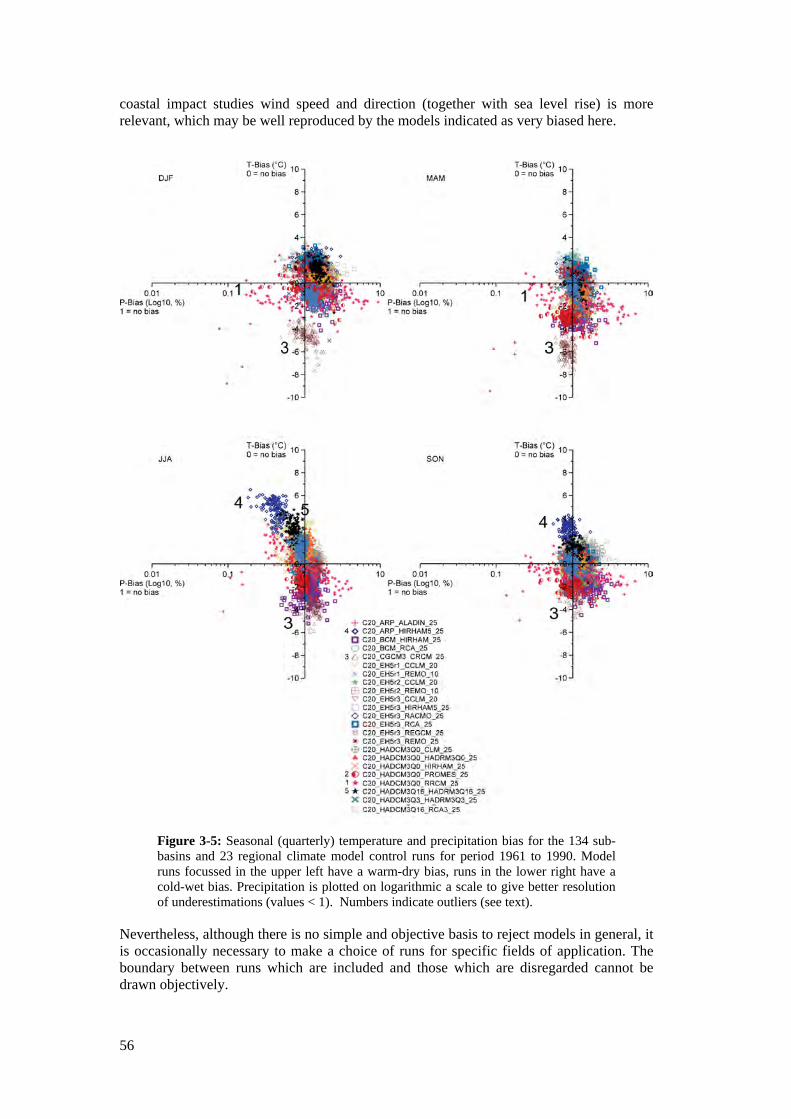
56
coastal impact studies wind speed and direction (together with sea level rise) is more relevant, which may be well reproduced by the models indicated as very biased here.
Figure 3-5: Seasonal (quarterly) temperature and precipitation bias for the 134 sub-basins and 23 regional climate model control runs for period 1961 to 1990. Model runs focussed in the upper left have a warm-dry bias, runs in the lower right have a cold-wet bias. Precipitation is plotted on logarithmic a scale to give better resolution of underestimations (values < 1). Numbers indicate outliers (see text).
Nevertheless, although there is no simple and objective basis to reject models in general, it is occasionally necessary to make a choice of runs for specific fields of application. The boundary between runs which are included and those which are disregarded cannot be drawn objectively.
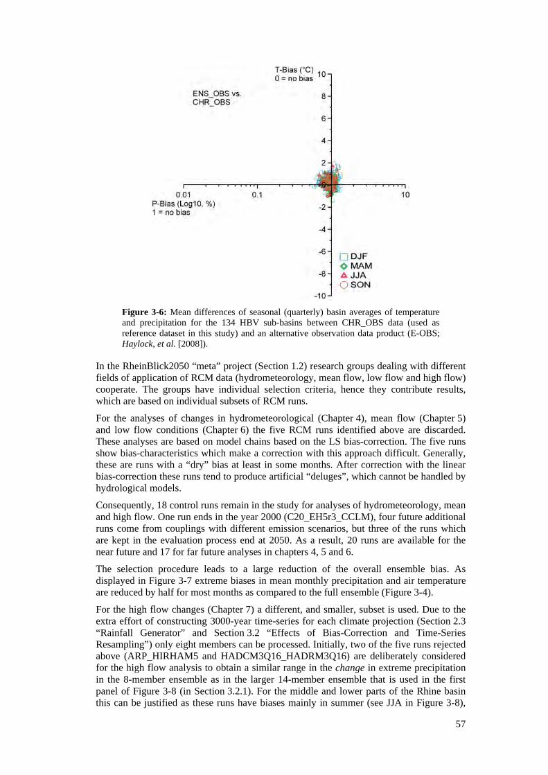
57
Figure 3-6: Mean differences of seasonal (quarterly) basin averages of temperature and precipitation for the 134 HBV sub-basins between CHR_OBS data (used as reference dataset in this study) and an alternative observation data product (E-OBS; Haylock, et al. [2008]).
In the RheinBlick2050 “meta” project (Section 1.2) research groups dealing with different fields of application of RCM data (hydrometeorology, mean flow, low flow and high flow) cooperate. The groups have individual selection criteria, hence they contribute results, which are based on individual subsets of RCM runs.
For the analyses of changes in hydrometeorological (Chapter 4), mean flow (Chapter 5) and low flow conditions (Chapter 6) the five RCM runs identified above are discarded. These analyses are based on model chains based on the LS bias-correction. The five runs show bias-characteristics which make a correction with this approach difficult. Generally, these are runs with a “dry” bias at least in some months. After correction with the linear bias-correction these runs tend to produce artificial “deluges”, which cannot be handled by hydrological models.
Consequently, 18 control runs remain in the study for analyses of hydrometeorology, mean and high flow. One run ends in the year 2000 (C20_EH5r3_CCLM), four future additional runs come from couplings with different emission scenarios, but three of the runs which are kept in the evaluation process end at 2050. As a result, 20 runs are available for the near future and 17 for far future analyses in chapters 4, 5 and 6.
The selection procedure leads to a large reduction of the overall ensemble bias. As displayed in Figure 3-7 extreme biases in mean monthly precipitation and air temperature are reduced by half for most months as compared to the full ensemble (Figure 3-4).
For the high flow changes (Chapter 7) a different, and smaller, subset is used. Due to the extra effort of constructing 3000-year time-series for each climate projection (Section 2.3 “Rainfall Generator” and Section 3.2 “Effects of Bias-Correction and Time-Series Resampling”) only eight members can be processed. Initially, two of the five runs rejected above (ARP_HIRHAM5 and HADCM3Q16_HADRM3Q16) are deliberately considered for the high flow analysis to obtain a similar range in the change in extreme precipitation in the 8-member ensemble as in the larger 14-member ensemble that is used in the first panel of Figure 3-8 (in Section 3.2.1). For the middle and lower parts of the Rhine basin this can be justified as these runs have biases mainly in summer (see JJA in Figure 3-8),
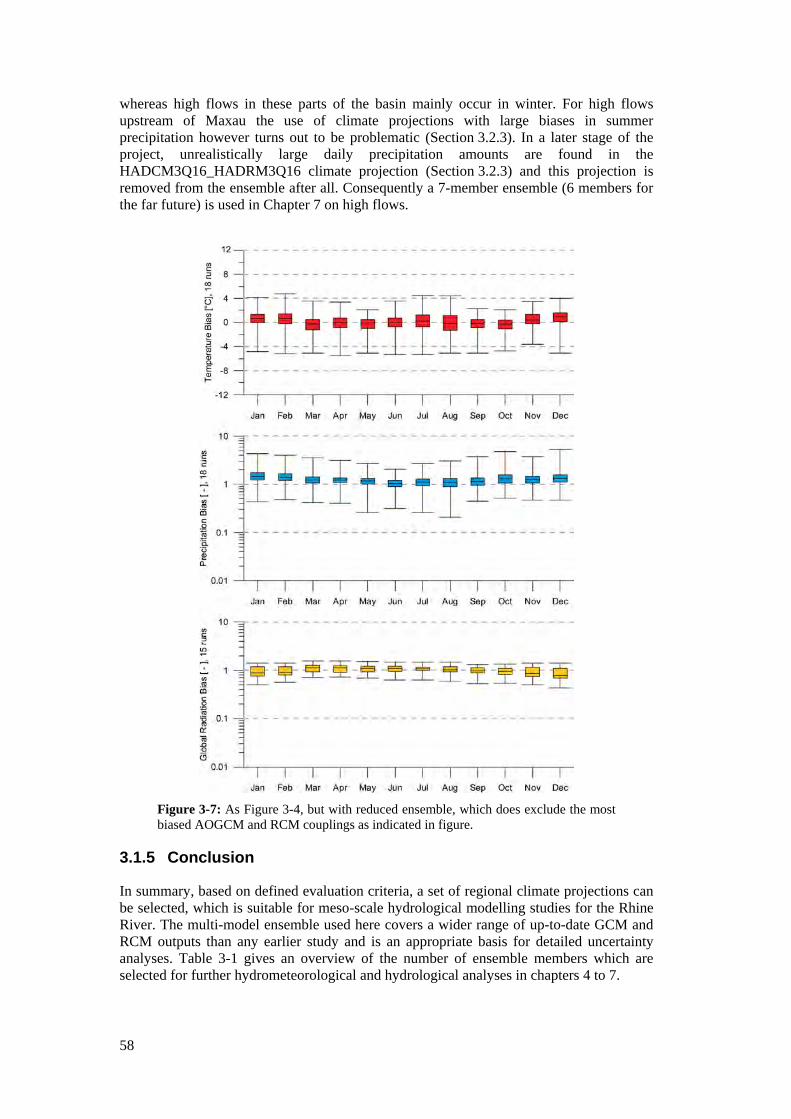
58
whereas high flows in these parts of the basin mainly occur in winter. For high flows upstream of Maxau the use of climate projections with large biases in summer precipitation however turns out to be problematic (Section 3.2.3). In a later stage of the project, unrealistically large daily precipitation amounts are found in the HADCM3Q16_HADRM3Q16 climate projection (Section 3.2.3) and this projection is removed from the ensemble after all. Consequently a 7-member ensemble (6 members for the far future) is used in Chapter 7 on high flows.
Figure 3-7: As Figure 3-4, but with reduced ensemble, which does exclude the most biased AOGCM and RCM couplings as indicated in figure.
3.1.5 Conclusion
In summary, based on defined evaluation criteria, a set of regional climate projections can be selected, which is suitable for meso-scale hydrological modelling studies for the Rhine River. The multi-model ensemble used here covers a wider range of up-to-date GCM and RCM outputs than any earlier study and is an appropriate basis for detailed uncertainty analyses. Table 3-1 gives an overview of the number of ensemble members which are selected for further hydrometeorological and hydrological analyses in chapters 4 to 7.
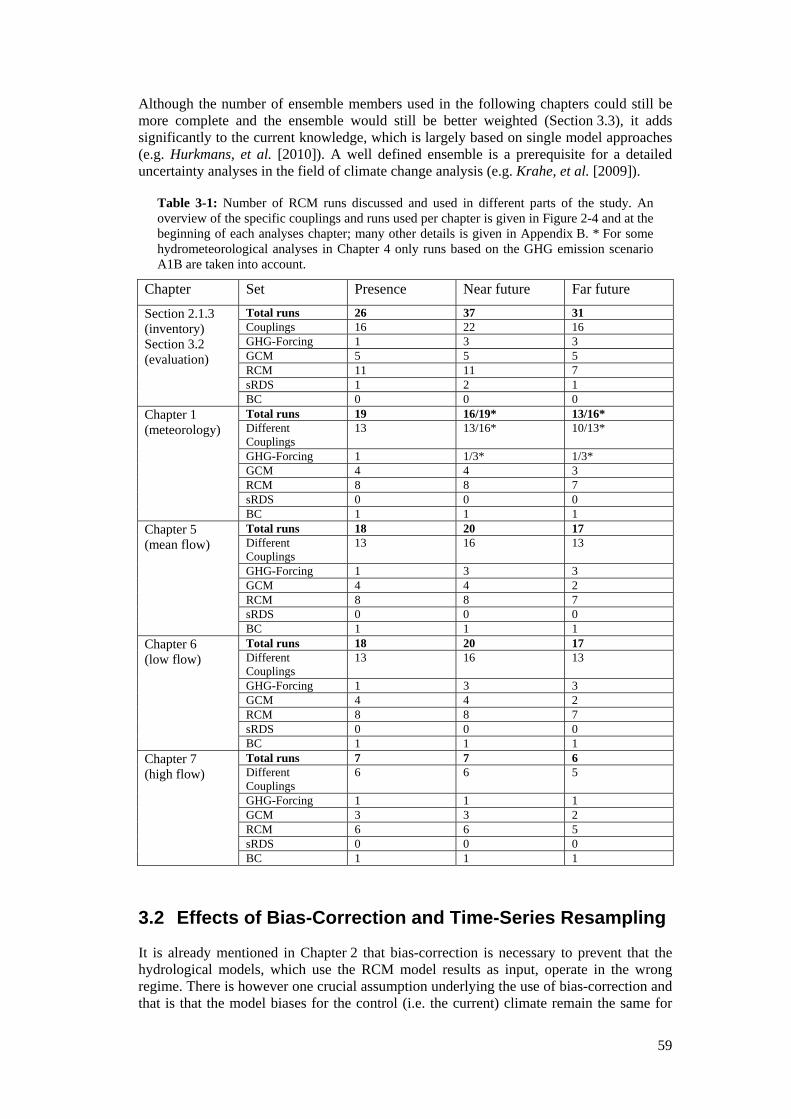
59
Although the number of ensemble members used in the following chapters could still be more complete and the ensemble would still be better weighted (Section 3.3), it adds significantly to the current knowledge, which is largely based on single model approaches (e.g. Hurkmans, et al. [2010]). A well defined ensemble is a prerequisite for a detailed uncertainty analyses in the field of climate change analysis (e.g. Krahe, et al. [2009]).
Table 3-1: Number of RCM runs discussed and used in different parts of the study. An overview of the specific couplings and runs used per chapter is given in Figure 2-4 and at the beginning of each analyses chapter; many other details is given in Appendix B. * For some hydrometeorological analyses in Chapter 4 only runs based on the GHG emission scenario A1B are taken into account.
Chapter Set Presence Near future Far future
Section 2.1.3 (inventory) Section 3.2 (evaluation)
Total runs 26 37 31 Couplings 16 22 16 GHG-Forcing 1 3 3 GCM 5 5 5 RCM 11 11 7 sRDS 1 2 1 BC 0 0 0
Chapter 1 (meteorology)
Total runs 19 16/19* 13/16* Different Couplings
13 13/16* 10/13*
GHG-Forcing 1 1/3* 1/3* GCM 4 4 3 RCM 8 8 7 sRDS 0 0 0 BC 1 1 1
Chapter 5 (mean flow)
Total runs 18 20 17 Different Couplings
13 16 13
GHG-Forcing 1 3 3 GCM 4 4 2 RCM 8 8 7 sRDS 0 0 0 BC 1 1 1
Chapter 6 (low flow)
Total runs 18 20 17 Different Couplings
13 16 13
GHG-Forcing 1 3 3 GCM 4 4 2 RCM 8 8 7 sRDS 0 0 0 BC 1 1 1
Chapter 7 (high flow)
Total runs 7 7 6 Different Couplings
6 6 5
GHG-Forcing 1 1 1 GCM 3 3 2 RCM 6 6 5 sRDS 0 0 0 BC 1 1 1
3.2 Effects of Bias-Correction and Time-Series Resampling
It is already mentioned in Chapter 2 that bias-correction is necessary to prevent that the hydrological models, which use the RCM model results as input, operate in the wrong regime. There is however one crucial assumption underlying the use of bias-correction and that is that the model biases for the control (i.e. the current) climate remain the same for
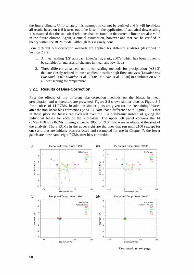
60
the future climate. Unfortunately this assumption cannot be verified and it will invalidate all results based on it if it turns out to be false. In the application of statistical downscaling it is assumed that the statistical relations that are found in the current climate are also valid in the future climate. Again, a crucial assumption, however one that can be verified in theory within the RCM model, although this is rarely done.
Four different bias-correction methods are applied for different analyses (described in Section 2.2.2):
1. A linear scaling (LS) approach [Lenderink, et al., 2007a] which has been proven to be suitable for analyses of changes in mean and low flows.
2. Three different advanced, non-linear scaling methods for precipitation (AS1-3) that are closely related to those applied in earlier high flow analyses [Leander and Buishand, 2007; Leander, et al., 2008; Te Linde, et al., 2010] in combination with a linear scaling for temperature.
3.2.1 Results of Bias-Correction
First the effects of the different bias-correction methods on the biases in mean precipitation and temperature are presented. Figure 3-8 shows similar plots as Figure 3-5 for a subset of 14 RCMs. In addition similar plots are given for the “remaining” biases after the non-linear bias-corrections (AS1-3). Note that a difference with Figure 3-5 is that in these plots the biases are averaged over the 134 sub-basins instead of giving the individual biases for each of the sub-basins. The upper left panel contains the 14 (ENSEMBLES) RCMs running either to 2050 or 2100 that were available at the start of the analysis. The 8 RCMs in the upper right are the ones that run until 2100 (except for one) and that are initially bias-corrected and resampled for use in Chapter 7, the lower panels are these same eight RCMs after bias-correction.
Continued on next page.
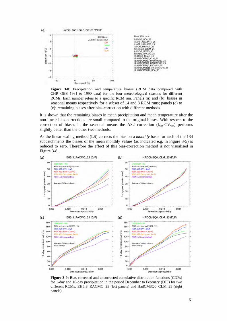
61
Figure 3-8: Precipitation and temperature biases (RCM data compared with CHR_OBS 1961 to 1990 data) for the four meteorological seasons for different RCMs. Each number refers to a specific RCM run. Panels (a) and (b): biases in seasonal means respectively for a subset of 14 and 8 RCM runs; panels (c) to (e): remaining biases after bias-correction with different methods.
It is shown that the remaining biases in mean precipitation and mean temperature after the non-linear bias-corrections are small compared to the original biases. With respect to the correction of biases in the seasonal means the AS2 correction (fwet-CVwet) performs slightly better than the other two methods.
As the linear scaling method (LS) corrects the bias on a monthly basis for each of the 134 subcatchments the biases of the mean monthly values (as indicated e.g. in Figure 3-5) is reduced to zero. Therefore the effect of this bias-correction method is not visualised in Figure 3-8.
Figure 3-9: Bias-corrected and uncorrected cumulative distribution functions (CDFs) for 1-day and 10-day precipitation in the period December to February (DJF) for two different RCMs: EH5r3_RACMO_25 (left panels) and HadCM3Q0_CLM_25 (right panels).
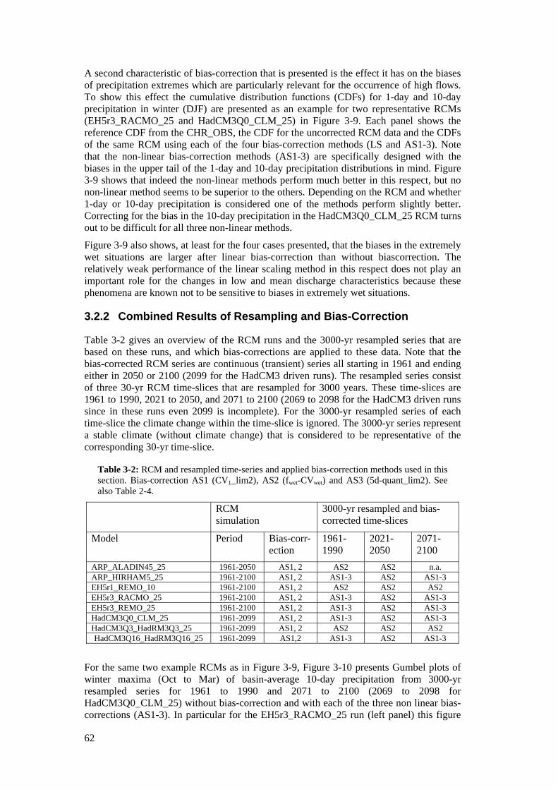
62
A second characteristic of bias-correction that is presented is the effect it has on the biases of precipitation extremes which are particularly relevant for the occurrence of high flows. To show this effect the cumulative distribution functions (CDFs) for 1-day and 10-day precipitation in winter (DJF) are presented as an example for two representative RCMs (EH5r3_RACMO_25 and HadCM3Q0_CLM_25) in Figure 3-9. Each panel shows the reference CDF from the CHR_OBS, the CDF for the uncorrected RCM data and the CDFs of the same RCM using each of the four bias-correction methods (LS and AS1-3). Note that the non-linear bias-correction methods (AS1-3) are specifically designed with the biases in the upper tail of the 1-day and 10-day precipitation distributions in mind. Figure 3-9 shows that indeed the non-linear methods perform much better in this respect, but no non-linear method seems to be superior to the others. Depending on the RCM and whether 1-day or 10-day precipitation is considered one of the methods perform slightly better. Correcting for the bias in the 10-day precipitation in the HadCM3Q0_CLM_25 RCM turns out to be difficult for all three non-linear methods.
Figure 3-9 also shows, at least for the four cases presented, that the biases in the extremely wet situations are larger after linear bias-correction than without biascorrection. The relatively weak performance of the linear scaling method in this respect does not play an important role for the changes in low and mean discharge characteristics because these phenomena are known not to be sensitive to biases in extremely wet situations.
3.2.2 Combined Results of Resampling and Bias-Correction
Table 3-2 gives an overview of the RCM runs and the 3000-yr resampled series that are based on these runs, and which bias-corrections are applied to these data. Note that the bias-corrected RCM series are continuous (transient) series all starting in 1961 and ending either in 2050 or 2100 (2099 for the HadCM3 driven runs). The resampled series consist of three 30-yr RCM time-slices that are resampled for 3000 years. These time-slices are 1961 to 1990, 2021 to 2050, and 2071 to 2100 (2069 to 2098 for the HadCM3 driven runs since in these runs even 2099 is incomplete). For the 3000-yr resampled series of each time-slice the climate change within the time-slice is ignored. The 3000-yr series represent a stable climate (without climate change) that is considered to be representative of the corresponding 30-yr time-slice.
Table 3-2: RCM and resampled time-series and applied bias-correction methods used in this section. Bias-correction AS1 (CV1_lim2), AS2 (fwet-CVwet) and AS3 (5d-quant_lim2). See also Table 2-4.
RCM simulation
3000-yr resampled and bias-corrected time-slices
Model Period Bias-corr-ection
1961-1990
2021-2050
2071-2100
ARP_ALADIN45_25 1961-2050 AS1, 2 AS2 AS2 n.a. ARP_HIRHAM5_25 1961-2100 AS1, 2 AS1-3 AS2 AS1-3 EH5r1_REMO_10 1961-2100 AS1, 2 AS2 AS2 AS2 EH5r3_RACMO_25 1961-2100 AS1, 2 AS1-3 AS2 AS1-3 EH5r3_REMO_25 1961-2100 AS1, 2 AS1-3 AS2 AS1-3 HadCM3Q0_CLM_25 1961-2099 AS1, 2 AS1-3 AS2 AS1-3 HadCM3Q3_HadRM3Q3_25 1961-2099 AS1, 2 AS2 AS2 AS2 HadCM3Q16_HadRM3Q16_25 1961-2099 AS1,2 AS1-3 AS2 AS1-3
For the same two example RCMs as in Figure 3-9, Figure 3-10 presents Gumbel plots of winter maxima (Oct to Mar) of basin-average 10-day precipitation from 3000-yr resampled series for 1961 to 1990 and 2071 to 2100 (2069 to 2098 for HadCM3Q0_CLM_25) without bias-correction and with each of the three non linear bias-corrections (AS1-3). In particular for the EH5r3_RACMO_25 run (left panel) this figure
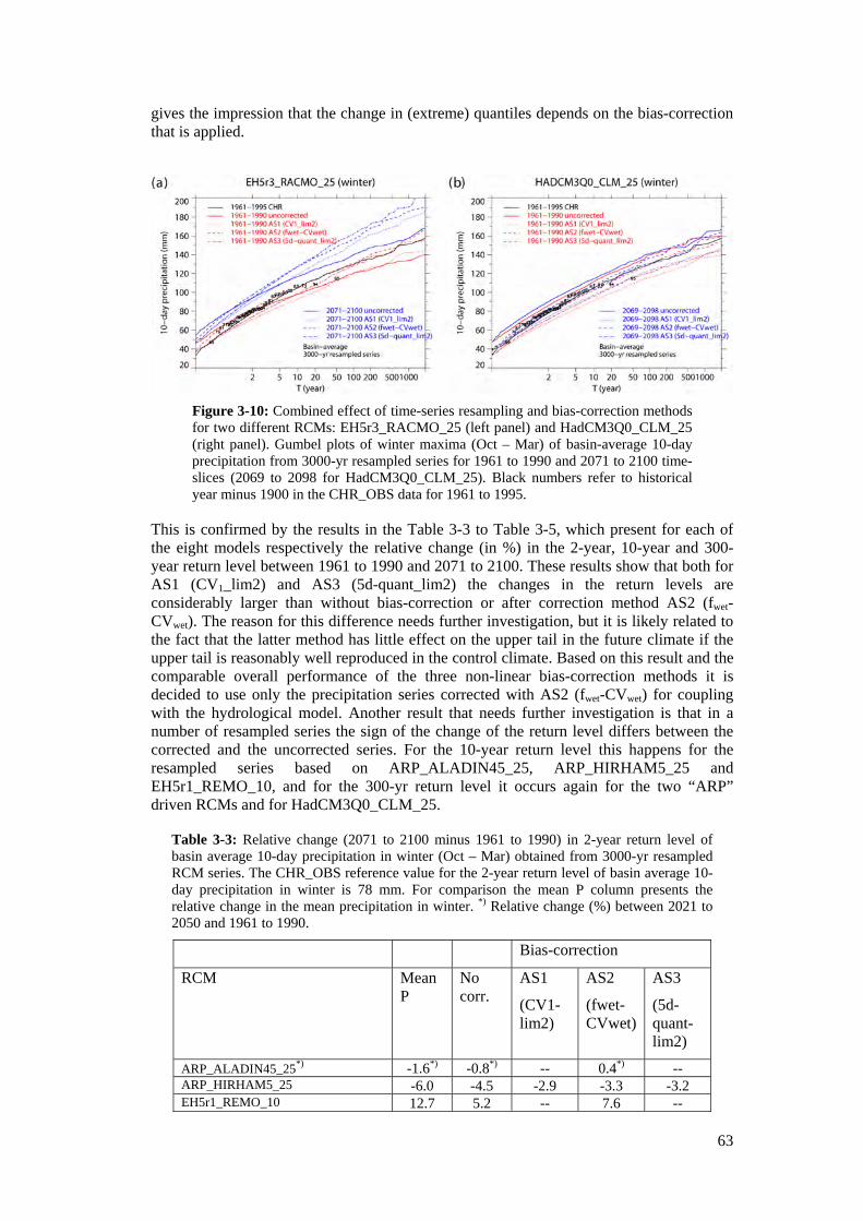
63
gives the impression that the change in (extreme) quantiles depends on the bias-correction that is applied.
Figure 3-10: Combined effect of time-series resampling and bias-correction methods for two different RCMs: EH5r3_RACMO_25 (left panel) and HadCM3Q0_CLM_25 (right panel). Gumbel plots of winter maxima (Oct – Mar) of basin-average 10-day precipitation from 3000-yr resampled series for 1961 to 1990 and 2071 to 2100 time-slices (2069 to 2098 for HadCM3Q0_CLM_25). Black numbers refer to historical year minus 1900 in the CHR_OBS data for 1961 to 1995.
This is confirmed by the results in the Table 3-3 to Table 3-5, which present for each of the eight models respectively the relative change (in %) in the 2-year, 10-year and 300-year return level between 1961 to 1990 and 2071 to 2100. These results show that both for AS1 (CV1_lim2) and AS3 (5d-quant_lim2) the changes in the return levels are considerably larger than without bias-correction or after correction method AS2 (fwet-CVwet). The reason for this difference needs further investigation, but it is likely related to the fact that the latter method has little effect on the upper tail in the future climate if the upper tail is reasonably well reproduced in the control climate. Based on this result and the comparable overall performance of the three non-linear bias-correction methods it is decided to use only the precipitation series corrected with AS2 (fwet-CVwet) for coupling with the hydrological model. Another result that needs further investigation is that in a number of resampled series the sign of the change of the return level differs between the corrected and the uncorrected series. For the 10-year return level this happens for the resampled series based on ARP_ALADIN45_25, ARP_HIRHAM5_25 and EH5r1_REMO_10, and for the 300-yr return level it occurs again for the two “ARP” driven RCMs and for HadCM3Q0_CLM_25.
Table 3-3: Relative change (2071 to 2100 minus 1961 to 1990) in 2-year return level of basin average 10-day precipitation in winter (Oct – Mar) obtained from 3000-yr resampled RCM series. The CHR_OBS reference value for the 2-year return level of basin average 10-day precipitation in winter is 78 mm. For comparison the mean P column presents the relative change in the mean precipitation in winter. *) Relative change (%) between 2021 to 2050 and 1961 to 1990.
Bias-correction
RCM Mean P
No corr.
AS1
(CV1-lim2)
AS2
(fwet-CVwet)
AS3
(5d-quant-lim2)
ARP_ALADIN45_25*) -1.6*) -0.8*) -- 0.4*) -- ARP_HIRHAM5_25 -6.0 -4.5 -2.9 -3.3 -3.2 EH5r1_REMO_10 12.7 5.2 -- 7.6 --
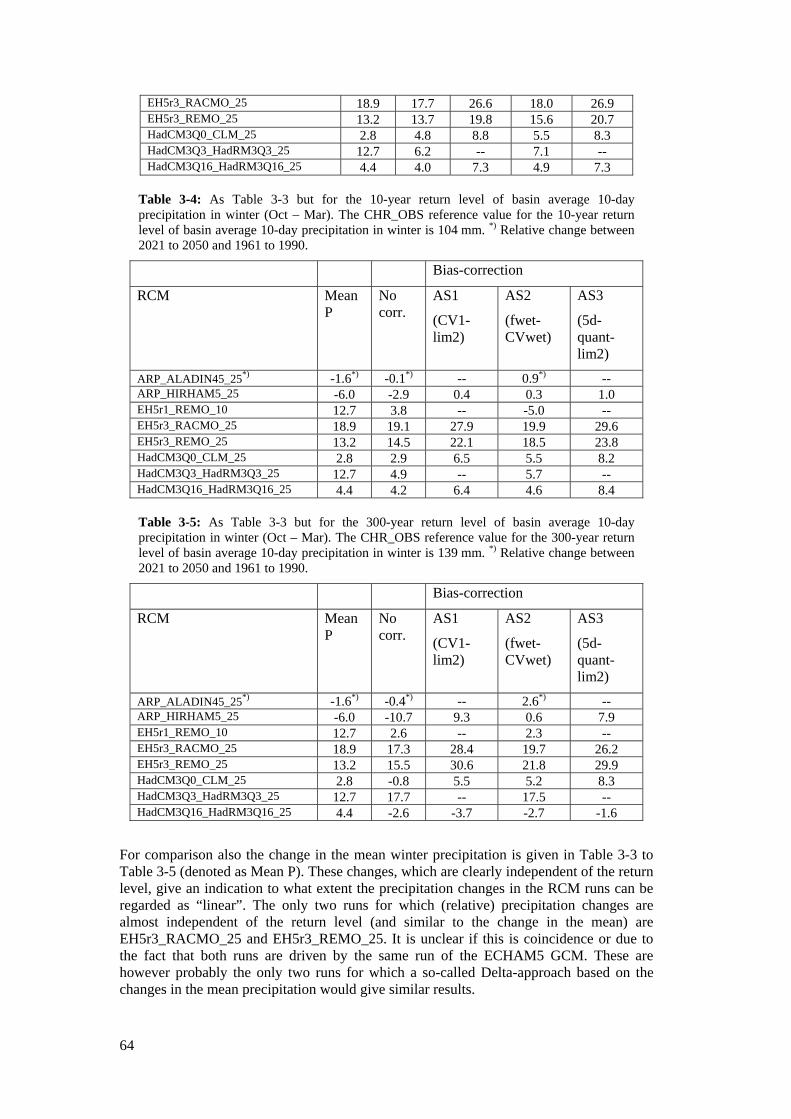
64
EH5r3_RACMO_25 18.9 17.7 26.6 18.0 26.9 EH5r3_REMO_25 13.2 13.7 19.8 15.6 20.7 HadCM3Q0_CLM_25 2.8 4.8 8.8 5.5 8.3 HadCM3Q3_HadRM3Q3_25 12.7 6.2 -- 7.1 -- HadCM3Q16_HadRM3Q16_25 4.4 4.0 7.3 4.9 7.3
Table 3-4: As Table 3-3 but for the 10-year return level of basin average 10-day precipitation in winter (Oct – Mar). The CHR_OBS reference value for the 10-year return level of basin average 10-day precipitation in winter is 104 mm. *) Relative change between 2021 to 2050 and 1961 to 1990.
Bias-correction
RCM Mean P
No corr.
AS1
(CV1-lim2)
AS2
(fwet-CVwet)
AS3
(5d-quant-lim2)
ARP_ALADIN45_25*) -1.6*) -0.1*) -- 0.9*) -- ARP_HIRHAM5_25 -6.0 -2.9 0.4 0.3 1.0 EH5r1_REMO_10 12.7 3.8 -- -5.0 -- EH5r3_RACMO_25 18.9 19.1 27.9 19.9 29.6 EH5r3_REMO_25 13.2 14.5 22.1 18.5 23.8 HadCM3Q0_CLM_25 2.8 2.9 6.5 5.5 8.2 HadCM3Q3_HadRM3Q3_25 12.7 4.9 -- 5.7 -- HadCM3Q16_HadRM3Q16_25 4.4 4.2 6.4 4.6 8.4
Table 3-5: As Table 3-3 but for the 300-year return level of basin average 10-day precipitation in winter (Oct – Mar). The CHR_OBS reference value for the 300-year return level of basin average 10-day precipitation in winter is 139 mm. *) Relative change between 2021 to 2050 and 1961 to 1990.
Bias-correction
RCM Mean P
No corr.
AS1
(CV1-lim2)
AS2
(fwet-CVwet)
AS3
(5d-quant-lim2)
ARP_ALADIN45_25*) -1.6*) -0.4*) -- 2.6*) -- ARP_HIRHAM5_25 -6.0 -10.7 9.3 0.6 7.9 EH5r1_REMO_10 12.7 2.6 -- 2.3 -- EH5r3_RACMO_25 18.9 17.3 28.4 19.7 26.2 EH5r3_REMO_25 13.2 15.5 30.6 21.8 29.9 HadCM3Q0_CLM_25 2.8 -0.8 5.5 5.2 8.3 HadCM3Q3_HadRM3Q3_25 12.7 17.7 -- 17.5 -- HadCM3Q16_HadRM3Q16_25 4.4 -2.6 -3.7 -2.7 -1.6
For comparison also the change in the mean winter precipitation is given in Table 3-3 to Table 3-5 (denoted as Mean P). These changes, which are clearly independent of the return level, give an indication to what extent the precipitation changes in the RCM runs can be regarded as “linear”. The only two runs for which (relative) precipitation changes are almost independent of the return level (and similar to the change in the mean) are EH5r3_RACMO_25 and EH5r3_REMO_25. It is unclear if this is coincidence or due to the fact that both runs are driven by the same run of the ECHAM5 GCM. These are however probably the only two runs for which a so-called Delta-approach based on the changes in the mean precipitation would give similar results.
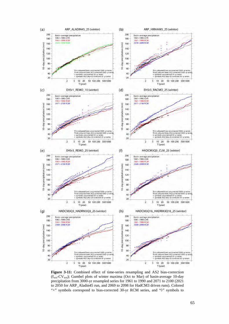
65
Figure 3-11: Combined effect of time-series resampling and AS2 bias-correction (fwet-CVwet); Gumbel plots of winter maxima (Oct to Mar) of basin-average 10-day precipitation from 3000-yr resampled series for 1961 to 1990 and 2071 to 2100 (2021 to 2050 for ARP_Aladin45 run, and 2069 to 2098 for HadCM3 driven runs). Colored “+” symbols correspond to bias-corrected 30-yr RCM series, and “◊” symbols to
66
uncorrected (original) 30-yr RCM series. Black numbers refer to historical year minus 1900 in CHR_OBS data. Thin lines correspond to the uncorrected resampled series.
Figure 3-11 is similar to Figure 3-10 and summarises all available 3000-yr resampled series based on these 8 RCM runs, in terms of winter maxima of basin-average 10-day precipitation, bias-corrected with AS2 (Fwet_CVwet) for coupling with the hydrological model for high-flow studies (discussed in Chapter 7). In these diagrams also the winter maxima for the underlying 30-yr RCM time-slices are shown. These plots therefore present both, the effect of resampling and bias-correction. From these plots it is concluded that, both for the 1961 to 1990 RCM series and the corresponding 3000-yr resampled RCM series, the distributions of the maximum basin-average 10-day precipitation in the hydrological winter from the AS2 bias-corrected RCM series are much closer to the distributions from the CHR_OBS series than those from the uncorrected RCM series are.
3.2.3 Limitations of the Bias-Corrected Resampled Series
After coupling the bias-corrected RCM projections to the hydrological model some peculiar results are found in the simulated discharges; in particular with respect to the high flow statistics as discussed in Chapter 7.
First, unrealistically large daily precipitation values are found in the HADCM3Q16_HADRM3Q16 climate projection. Second, systematic differences between extreme flow statistics based on the bias-corrected RCM reference period (1961 to 1990) and those based on CHR_OBS were found from Basel to Worms. These two problems and their consequences are discussed in more detail in this subsection.
Unrealistically large daily precipitation values in HADCM3Q16_HADRM3Q16 For one day in August 2035 extremely large precipitation amounts are simulated in large parts of Main basin in the HADCM3Q16_HADRM3Q16 run. Another unusual daily precipitation amount is simulated in July 2037 affecting a large part of the Moselle basin. For individual sub-basins the largest daily amounts on these days lie between 100 mm and 230 mm and the daily precipitation averaged over these (large) basins is over 70 mm in both cases. These basin-average amounts are approximately twice as large as the largest value observed in the CHR_OBS data for the period 1961 to 1995 for these respective basins. These simulated events are therefore considered highly unlikely.
In the resampling and bias-correction procedure these large amounts are even further enhanced up to basin-average amounts of about 100 mm. In the 3000-yr resampled series from the 2021 to 2050 time-slice several of such days are simulated. In the most extreme 10-day periods in the 3000-yr series probably one of these 2 days is resampled 2 or 3 times leading to a largest basin-average 10-day amount of 289 mm for the Moselle and 395 mm for the Main basin. It will be no surprise that these events lead to unprecedented and unrealistic discharge events at respectively Raunheim and Trier, and consequently also at Kaub, Köln and Lobith. This makes it very difficult to derive reliable extreme flow statistics for these locations. Therefore it is decided not to use the results from the HADCM3Q16_HADRM3Q16 run to determine the scenario bandwidths and tendencies for the extreme flow statistics presented in Chapter 7.
Systematic differences in high flows from Basel to Worms For Basel, Maxau and Worms systematic differences are found in high flow statistics between the hydrological model forced with the CHR_OBS data and those driven by the bias-corrected (and, for HQ100 and HQ1000, resampled) climate model data for the 1961 to 1990 period. The results based on the bias-corrected climate model data are
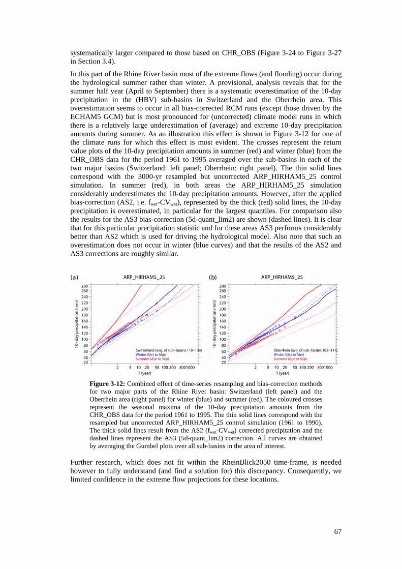
67
systematically larger compared to those based on CHR_OBS (Figure 3-24 to Figure 3-27 in Section 3.4).
In this part of the Rhine River basin most of the extreme flows (and flooding) occur during the hydrological summer rather than winter. A provisional, analysis reveals that for the summer half year (April to September) there is a systematic overestimation of the 10-day precipitation in the (HBV) sub-basins in Switzerland and the Oberrhein area. This overestimation seems to occur in all bias-corrected RCM runs (except those driven by the ECHAM5 GCM) but is most pronounced for (uncorrected) climate model runs in which there is a relatively large underestimation of (average) and extreme 10-day precipitation amounts during summer. As an illustration this effect is shown in Figure 3-12 for one of the climate runs for which this effect is most evident. The crosses represent the return value plots of the 10-day precipitation amounts in summer (red) and winter (blue) from the CHR_OBS data for the period 1961 to 1995 averaged over the sub-basins in each of the two major basins (Switzerland: left panel; Oberrhein: right panel). The thin solid lines correspond with the 3000-yr resampled but uncorrected ARP_HIRHAM5_25 control simulation. In summer (red), in both areas the ARP_HIRHAM5_25 simulation considerably underestimates the 10-day precipitation amounts. However, after the applied bias-correction (AS2, i.e. fwet-CVwet), represented by the thick (red) solid lines, the 10-day precipitation is overestimated, in particular for the largest quantiles. For comparison also the results for the AS3 bias-correction (5d-quant_lim2) are shown (dashed lines). It is clear that for this particular precipitation statistic and for these areas AS3 performs considerably better than AS2 which is used for driving the hydrological model. Also note that such an overestimation does not occur in winter (blue curves) and that the results of the AS2 and AS3 corrections are roughly similar.
Figure 3-12: Combined effect of time-series resampling and bias-correction methods for two major parts of the Rhine River basin: Switzerland (left panel) and the Oberrhein area (right panel) for winter (blue) and summer (red). The coloured crosses represent the seasonal maxima of the 10-day precipitation amounts from the CHR_OBS data for the period 1961 to 1995. The thin solid lines correspond with the resampled but uncorrected ARP_HIRHAM5_25 control simulation (1961 to 1990). The thick solid lines result from the AS2 (fwet-CVwet) corrected precipitation and the dashed lines represent the AS3 (5d-quant_lim2) correction. All curves are obtained by averaging the Gumbel plots over all sub-basins in the area of interest.
Further research, which does not fit within the RheinBlick2050 time-frame, is needed however to fully understand (and find a solution for) this discrepancy. Consequently, we limited confidence in the extreme flow projections for these locations.
68
3.2.4 Conclusions
In this section we look at specific results of bias-correction and of the combination of time-series resampling and bias-correction. Overall it is concluded that the LS bias-correction is suitable for correcting the mean which is relevant for the analyses of mean and low flows. Apart from an imperfection in Switzerland and the Oberrhein in the hydrological summer, the AS2 correction is most suitable for correcting biases in extreme (multi-day) precipitation as well, which is particularly relevant for the analysis of high flow changes. In more detail it is concluded that:
(1) The relative changes in the 2-, 10- and 300-yr return levels of the maximum basin-average 10-day precipitation in the hydrological winter after bias-correction method AS2 are most similar to the changes in these return levels without bias-correction. With the other two non-linear bias-correction methods the changes in these return levels are sometimes considerably larger. The reason for this difference needs further investigation. It is therefore decided to use the AS2 bias-correction in combination with the hydrological simulations relevant for Chapter 7 (“High Flow Changes in the Rhine River Basin”).
(2) The distributions of the maximum basin-average 10-day precipitation in the hydrological winter from the AS2 bias-corrected RCM series are much closer to the distributions from the CHR_OBS series than those from the uncorrected RCM series are. This holds for the original 1961 to 1990 RCM series as well as the corresponding 3000-yr resampled RCM series.
(3) In the hydrological summer, however, a systematic overestimation of the 10-day precipitation in Switzerland and the Oberrhein area is identified as a result of the applied AS2 bias-correction. This overestimation is most pronounced for RCM runs with a large “dry bias” in summer. Further research is, however, needed to fully understand (and find a solution for) this imperfection. Consequently, we have limited confidence in the high flow projections (in Chapter 7) for gauges Basel, Maxau and Worms.
Another result from this section is that unrealistically large daily precipitation amounts in large parts of the Moselle and Main basins were found in the HADCM3Q16_HADRM3Q16 projection. Since this largely affects the high flow statistics for the gauges Raunheim and Trier and consequently Kaub, Köln and Lobith this projection is removed from the ensemble used in Chapter 7.
3.3 Hydrological Model Performance and Uncertainty Analysis
This chapter discusses and quantifies the issue of uncertainty due to hydrological modelling in general and with special focus to the model versions selected for the impact assessment in the following chapters.
First, a comparative analysis of the reliability of hydrological models is performed using flow observations over the reference period. We use a set of statistical evaluation criteria which gives evidence of the specific performance in mean, low and high flow.
Second, a specific analysis is performed on the uncertainty linked to the stationarity hypothesis made on model parameters, using differential split sample tests.
Third, a quantification of relative importance of different model structures, different parameter sets and different input data for the overall uncertainty of flow simulations is made.
Fourth, we discuss the specific limitations of the model versions selected for the impact assessment in the following chapters.
69
Finally, we evaluate the ability of the complete model chains (consisting of C20-GHG-forcing, global and regional climate model, bias-correction and time-series-resampling and hydrological modelling) to reproduce observed discharge target measures.
3.3.1 Model Performance Evaluation over the Reference Period
Objectives The hydrological models that are be used in the modelling chain to derive flow simulations for the future period can be evaluated under current conditions since flow observations are available. This evaluation has two main objectives:
1. assessing the suitability of the selected models for the study catchments: the models should be able to represent the current hydrological behaviour of these catchments. If not, this would mean that the models miss some main features of the hydrological behaviour and therefore may not be considered as reliable;
2. quantify the uncertainty associated to the choice of the hydrological model: since several hydrological models are used in this study, this provides the opportunity to quantify the uncertainty associated with the hydrological modelling scheme. If all models outputs are very close to observations, this may indicate that the uncertainty due to choice of the model structure is limited. Else, the choice of a model may have important consequences on modelling results.
The performance of the hydrological models described in Section 2.4 is evaluated over the reference period, i.e. 1961 to 1990.
Data The models are driven by the same inputs over the study period, i.e. temperature and precipitation data from the reference observation dataset on the Rhine basin (CHR_OBS), which provides daily mean values over 134 sub-basins (see Figure 1-1). Two formulas are used to compute potential evapotranspiration (PE) estimates in the HBV134 model: the classical Penman-Wendling [ATV-DVWK, 2002] formula and the formula proposed by Oudin, et al. [2006] and based on temperature. The sensitivity to these two PE inputs is commented in the next sections.
The lumped models are fed with precipitation and temperature data averaged over each catchment area. Only the Oudin's formula is used in these models.
Parameter estimation The way parameters are calibrated differs between models:
- The HBV134 model is based on the model version described by Eberle, et al. [2005]. In this model, parameterization is the result of a process of expertise and was made in different phases. Several refinements are made in successive studies. Model parameters can be considered to be optimised over the 1961 to 1995 period. Therefore, in the following, the HBV134 model results are considered as calibration results. Note that three model versions are analysed for this model: the simulations produced by BfG using two different PE inputs (Oudin and Penman-Wendling) and the simulation produced by Deltares (see Section 2.4.2).
- The lumped models are calibrated using a local search procedure found efficient for this type of models. The procedure is described by Edijatno, et al. [1999]. As it is easy to perform a calibration for these models, we make two types of tests: (1) calibration over the whole reference period to have results directly comparable with the results of the HBV134 model; (2) calibration on each half of the reference period, with a validation on the independent sub-period each time, to build a
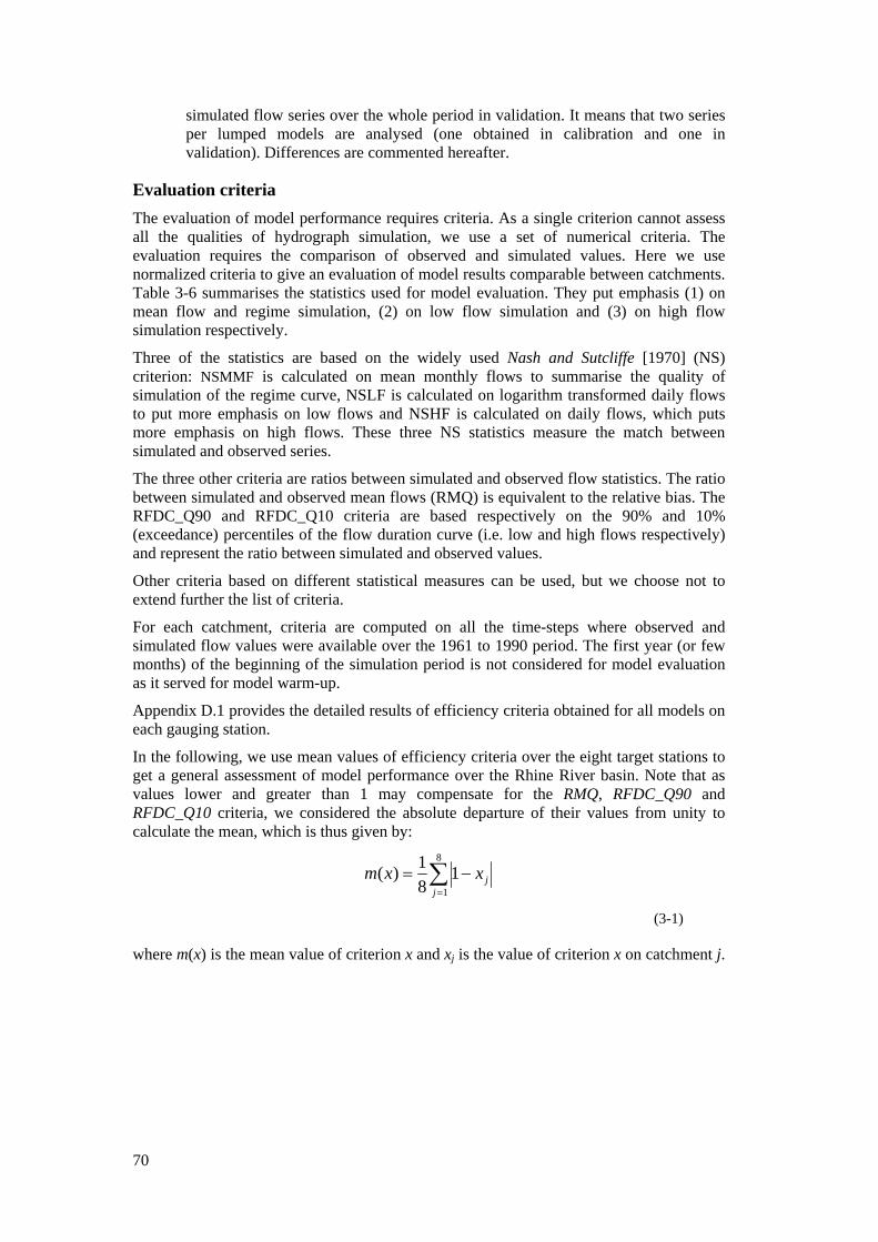
70
simulated flow series over the whole period in validation. It means that two series per lumped models are analysed (one obtained in calibration and one in validation). Differences are commented hereafter.
Evaluation criteria The evaluation of model performance requires criteria. As a single criterion cannot assess all the qualities of hydrograph simulation, we use a set of numerical criteria. The evaluation requires the comparison of observed and simulated values. Here we use normalized criteria to give an evaluation of model results comparable between catchments. Table 3-6 summarises the statistics used for model evaluation. They put emphasis (1) on mean flow and regime simulation, (2) on low flow simulation and (3) on high flow simulation respectively.
Three of the statistics are based on the widely used Nash and Sutcliffe [1970] (NS) criterion: NSMMF is calculated on mean monthly flows to summarise the quality of simulation of the regime curve, NSLF is calculated on logarithm transformed daily flows to put more emphasis on low flows and NSHF is calculated on daily flows, which puts more emphasis on high flows. These three NS statistics measure the match between simulated and observed series.
The three other criteria are ratios between simulated and observed flow statistics. The ratio between simulated and observed mean flows (RMQ) is equivalent to the relative bias. The RFDC_Q90 and RFDC_Q10 criteria are based respectively on the 90% and 10% (exceedance) percentiles of the flow duration curve (i.e. low and high flows respectively) and represent the ratio between simulated and observed values.
Other criteria based on different statistical measures can be used, but we choose not to extend further the list of criteria.
For each catchment, criteria are computed on all the time-steps where observed and simulated flow values were available over the 1961 to 1990 period. The first year (or few months) of the beginning of the simulation period is not considered for model evaluation as it served for model warm-up.
Appendix D.1 provides the detailed results of efficiency criteria obtained for all models on each gauging station.
In the following, we use mean values of efficiency criteria over the eight target stations to get a general assessment of model performance over the Rhine River basin. Note that as values lower and greater than 1 may compensate for the RMQ, RFDC_Q90 and RFDC_Q10 criteria, we considered the absolute departure of their values from unity to calculate the mean, which is thus given by:
∑=
−=8
11
81)(
jjxxm
(3-1)
where m(x) is the mean value of criterion x and xj is the value of criterion x on catchment j.
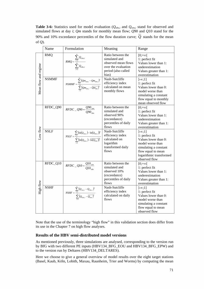
71
Table 3-6: Statistics used for model evaluation (Qobs,i and Qsim,i stand for observed and simulated flows at day i; Qm stands for monthly mean flow; Q90 and Q10 stand for the 90% and 10% exceedance percentiles of the flow duration curve; Q stands for the mean of Q).
Name Formulation Meaning Range
Mea
n flo
w a
nd re
gim
e
RMQ
∑
∑
=
== n
iiobs
n
iisim
Q
QRMQ
1,
1,
Ratio between the simulated and observed mean flows over the evaluation period (also called bias)
[0;+∞[ 1: perfect fit Values lower than 1: underestimation Values greater than 1: overestimation
NSMMF ( )
( )∑
∑
=
=
−
−= 12
1
2,
12
1
2,,
iobsiobs
iiobsisim
QmQm
QmQmNSMMF
Nash-Sutcliffe efficiency index calculated on mean monthly flows
]-∞;1] 1: perfect fit Values lower than 0: model worse than simulating a constant flow equal to monthly mean observed flow
Low
flow
RFDC_Q90 obs
sim
QRFDC9090
90_ = Ratio between the simulated and observed 90% (exceedance) percentiles of daily flows
[0;+∞[ 1: perfect fit Values lower than 1: underestimation Values greater than 1: overestimation
NSLF ( ) ( )( )
( ) ( )( )∑
∑
=
=
−
−= n
iobsiobs
n
iiobsisim
QQNSLF
1
2,
1
2,,
lnln
lnln
Nash-Sutcliffe efficiency index calculated on logarithm transformed daily flows
]-∞;1] 1: perfect fit Values lower than 0: model worse than simulating a constant flow equal to mean logarithmic transformed observed flow
Hig
h flo
w
RFDC_Q10 obs
sim
QRFDC1010
10_ = Ratio between the simulated and observed 10% (exceedance) percentiles of daily flows
[0;+∞[ 1: perfect fit Values lower than 1: underestimation Values greater than 1: overestimation
NSHF ( )
( )∑
∑
=
=
−
−=
n
iobsiobs
n
iiobsisim
QQNSHF
1
2
,
1
2,, Nash-Sutcliffe
efficiency index calculated on daily flows
]-∞;1] 1: perfect fit Values lower than 0: model worse than simulating a constant flow equal to mean observed flow
Note that the use of the terminology “high flow” in this validation section does differ from its use in the Chapter 7 on high flow analyses.
Results of the HBV semi-distributed model versions As mentioned previously, three simulations are analysed, corresponding to the version run by BfG with two different PE inputs (HBV134_BFG_EOU and HBV134_BFG_EPW) and to the version run by Deltares (HBV134_DELTARES).
Here we choose to give a general overview of model results over the eight target stations (Basel, Kaub, Köln, Lobith, Maxau, Raunheim, Trier and Worms) by computing the mean
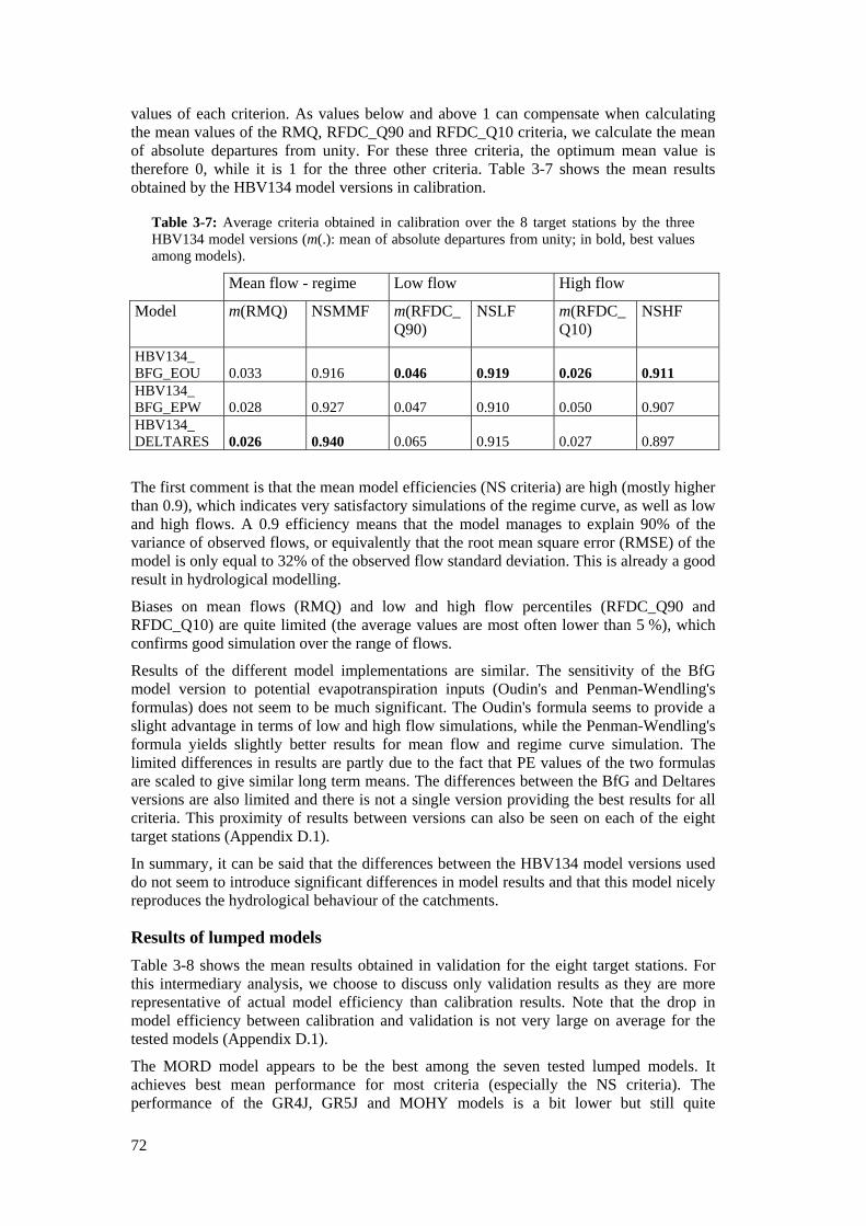
72
values of each criterion. As values below and above 1 can compensate when calculating the mean values of the RMQ, RFDC_Q90 and RFDC_Q10 criteria, we calculate the mean of absolute departures from unity. For these three criteria, the optimum mean value is therefore 0, while it is 1 for the three other criteria. Table 3-7 shows the mean results obtained by the HBV134 model versions in calibration.
Table 3-7: Average criteria obtained in calibration over the 8 target stations by the three HBV134 model versions (m(.): mean of absolute departures from unity; in bold, best values among models).
Mean flow - regime Low flow High flow
Model m(RMQ) NSMMF m(RFDC_Q90)
NSLF m(RFDC_Q10)
NSHF
HBV134_ BFG_EOU 0.033 0.916 0.046 0.919 0.026 0.911 HBV134_ BFG_EPW 0.028 0.927 0.047 0.910 0.050 0.907 HBV134_ DELTARES 0.026 0.940 0.065 0.915 0.027 0.897
The first comment is that the mean model efficiencies (NS criteria) are high (mostly higher than 0.9), which indicates very satisfactory simulations of the regime curve, as well as low and high flows. A 0.9 efficiency means that the model manages to explain 90% of the variance of observed flows, or equivalently that the root mean square error (RMSE) of the model is only equal to 32% of the observed flow standard deviation. This is already a good result in hydrological modelling.
Biases on mean flows (RMQ) and low and high flow percentiles (RFDC_Q90 and RFDC_Q10) are quite limited (the average values are most often lower than 5 %), which confirms good simulation over the range of flows.
Results of the different model implementations are similar. The sensitivity of the BfG model version to potential evapotranspiration inputs (Oudin's and Penman-Wendling's formulas) does not seem to be much significant. The Oudin's formula seems to provide a slight advantage in terms of low and high flow simulations, while the Penman-Wendling's formula yields slightly better results for mean flow and regime curve simulation. The limited differences in results are partly due to the fact that PE values of the two formulas are scaled to give similar long term means. The differences between the BfG and Deltares versions are also limited and there is not a single version providing the best results for all criteria. This proximity of results between versions can also be seen on each of the eight target stations (Appendix D.1).
In summary, it can be said that the differences between the HBV134 model versions used do not seem to introduce significant differences in model results and that this model nicely reproduces the hydrological behaviour of the catchments.
Results of lumped models Table 3-8 shows the mean results obtained in validation for the eight target stations. For this intermediary analysis, we choose to discuss only validation results as they are more representative of actual model efficiency than calibration results. Note that the drop in model efficiency between calibration and validation is not very large on average for the tested models (Appendix D.1).
The MORD model appears to be the best among the seven tested lumped models. It achieves best mean performance for most criteria (especially the NS criteria). The performance of the GR4J, GR5J and MOHY models is a bit lower but still quite
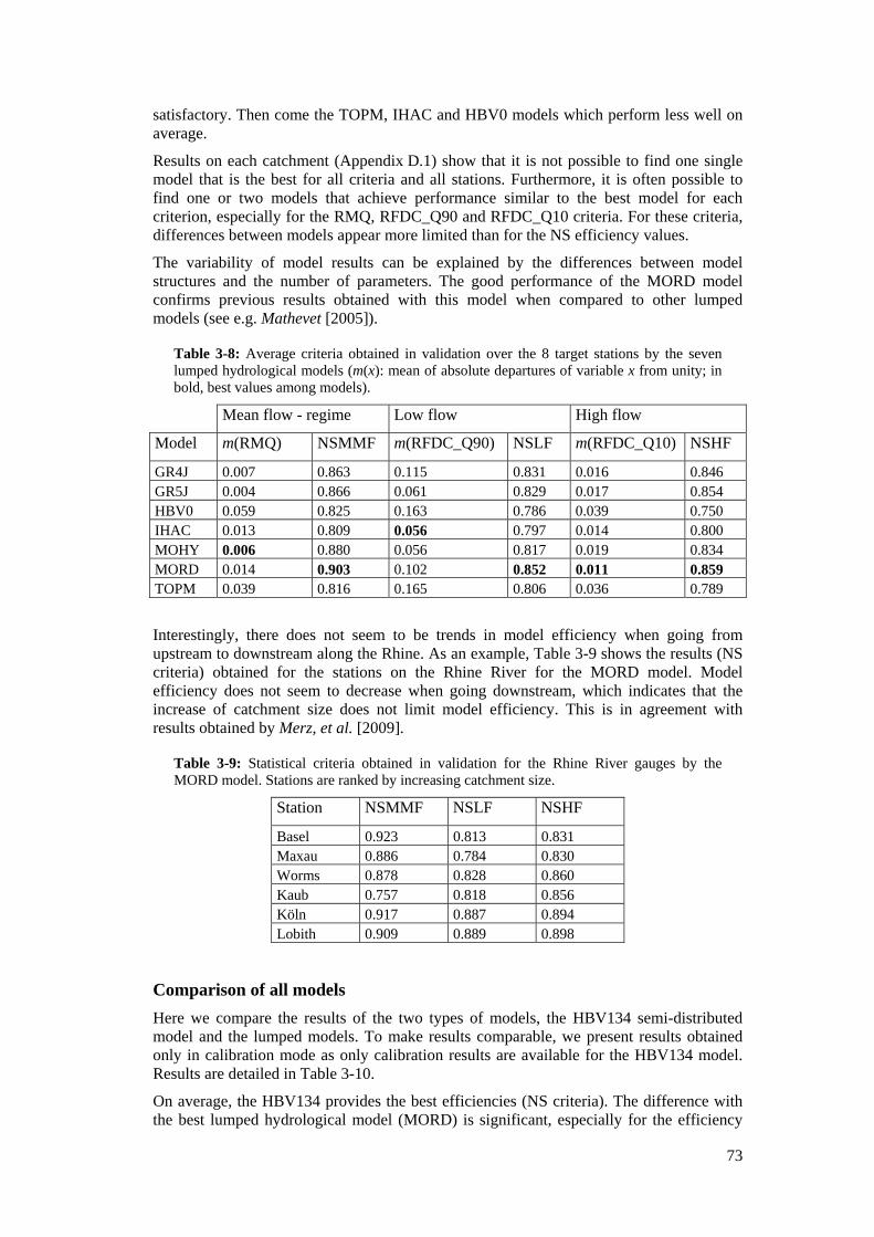
73
satisfactory. Then come the TOPM, IHAC and HBV0 models which perform less well on average.
Results on each catchment (Appendix D.1) show that it is not possible to find one single model that is the best for all criteria and all stations. Furthermore, it is often possible to find one or two models that achieve performance similar to the best model for each criterion, especially for the RMQ, RFDC_Q90 and RFDC_Q10 criteria. For these criteria, differences between models appear more limited than for the NS efficiency values.
The variability of model results can be explained by the differences between model structures and the number of parameters. The good performance of the MORD model confirms previous results obtained with this model when compared to other lumped models (see e.g. Mathevet [2005]).
Table 3-8: Average criteria obtained in validation over the 8 target stations by the seven lumped hydrological models (m(x): mean of absolute departures of variable x from unity; in bold, best values among models).
Mean flow - regime Low flow High flow
Model m(RMQ) NSMMF m(RFDC_Q90) NSLF m(RFDC_Q10) NSHF
GR4J 0.007 0.863 0.115 0.831 0.016 0.846 GR5J 0.004 0.866 0.061 0.829 0.017 0.854 HBV0 0.059 0.825 0.163 0.786 0.039 0.750 IHAC 0.013 0.809 0.056 0.797 0.014 0.800 MOHY 0.006 0.880 0.056 0.817 0.019 0.834 MORD 0.014 0.903 0.102 0.852 0.011 0.859 TOPM 0.039 0.816 0.165 0.806 0.036 0.789
Interestingly, there does not seem to be trends in model efficiency when going from upstream to downstream along the Rhine. As an example, Table 3-9 shows the results (NS criteria) obtained for the stations on the Rhine River for the MORD model. Model efficiency does not seem to decrease when going downstream, which indicates that the increase of catchment size does not limit model efficiency. This is in agreement with results obtained by Merz, et al. [2009].
Table 3-9: Statistical criteria obtained in validation for the Rhine River gauges by the MORD model. Stations are ranked by increasing catchment size.
Station NSMMF NSLF NSHF
Basel 0.923 0.813 0.831 Maxau 0.886 0.784 0.830 Worms 0.878 0.828 0.860 Kaub 0.757 0.818 0.856 Köln 0.917 0.887 0.894 Lobith 0.909 0.889 0.898
Comparison of all models Here we compare the results of the two types of models, the HBV134 semi-distributed model and the lumped models. To make results comparable, we present results obtained only in calibration mode as only calibration results are available for the HBV134 model. Results are detailed in Table 3-10.
On average, the HBV134 provides the best efficiencies (NS criteria). The difference with the best lumped hydrological model (MORD) is significant, especially for the efficiency
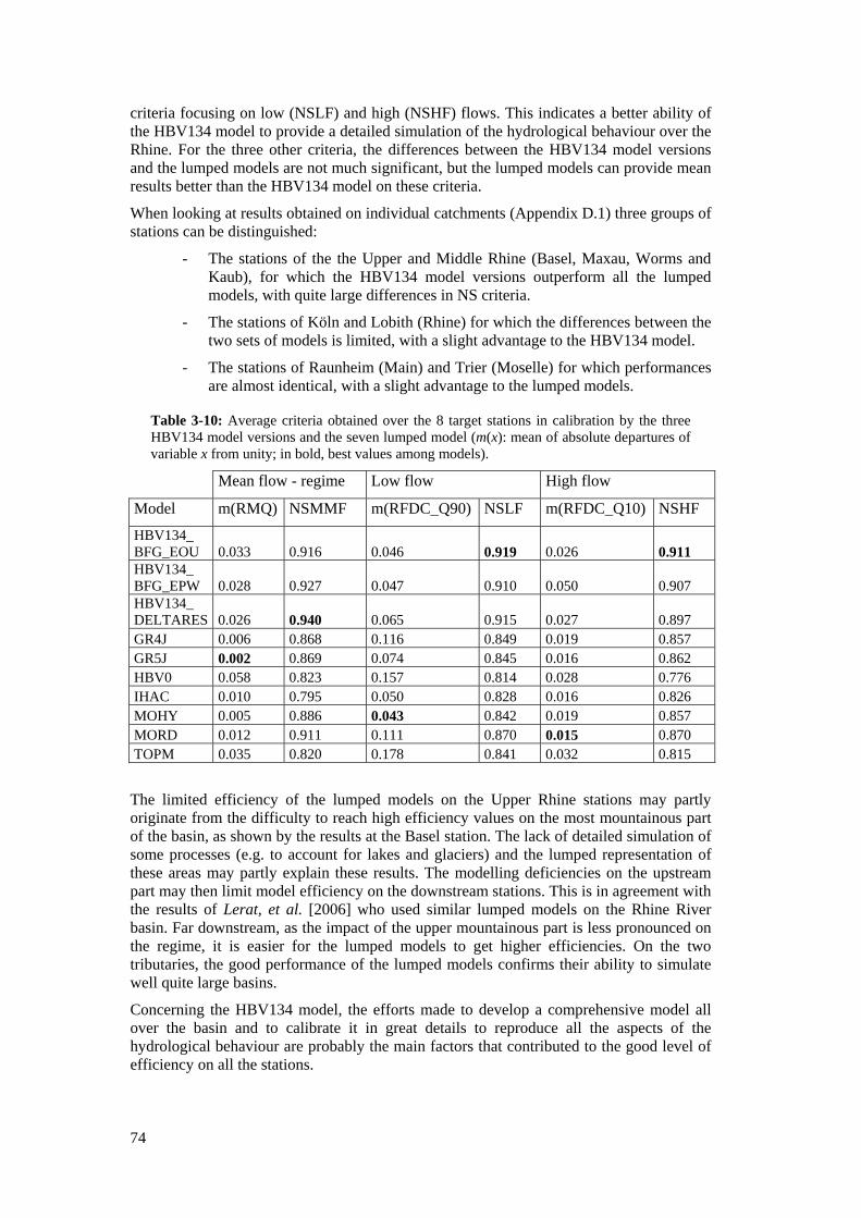
74
criteria focusing on low (NSLF) and high (NSHF) flows. This indicates a better ability of the HBV134 model to provide a detailed simulation of the hydrological behaviour over the Rhine. For the three other criteria, the differences between the HBV134 model versions and the lumped models are not much significant, but the lumped models can provide mean results better than the HBV134 model on these criteria.
When looking at results obtained on individual catchments (Appendix D.1) three groups of stations can be distinguished:
- The stations of the the Upper and Middle Rhine (Basel, Maxau, Worms and Kaub), for which the HBV134 model versions outperform all the lumped models, with quite large differences in NS criteria.
- The stations of Köln and Lobith (Rhine) for which the differences between the two sets of models is limited, with a slight advantage to the HBV134 model.
- The stations of Raunheim (Main) and Trier (Moselle) for which performances are almost identical, with a slight advantage to the lumped models.
Table 3-10: Average criteria obtained over the 8 target stations in calibration by the three HBV134 model versions and the seven lumped model (m(x): mean of absolute departures of variable x from unity; in bold, best values among models).
Mean flow - regime Low flow High flow
Model m(RMQ) NSMMF m(RFDC_Q90) NSLF m(RFDC_Q10) NSHF
HBV134_ BFG_EOU 0.033 0.916 0.046 0.919 0.026 0.911 HBV134_ BFG_EPW 0.028 0.927 0.047 0.910 0.050 0.907 HBV134_ DELTARES 0.026 0.940 0.065 0.915 0.027 0.897 GR4J 0.006 0.868 0.116 0.849 0.019 0.857 GR5J 0.002 0.869 0.074 0.845 0.016 0.862 HBV0 0.058 0.823 0.157 0.814 0.028 0.776 IHAC 0.010 0.795 0.050 0.828 0.016 0.826 MOHY 0.005 0.886 0.043 0.842 0.019 0.857 MORD 0.012 0.911 0.111 0.870 0.015 0.870 TOPM 0.035 0.820 0.178 0.841 0.032 0.815
The limited efficiency of the lumped models on the Upper Rhine stations may partly originate from the difficulty to reach high efficiency values on the most mountainous part of the basin, as shown by the results at the Basel station. The lack of detailed simulation of some processes (e.g. to account for lakes and glaciers) and the lumped representation of these areas may partly explain these results. The modelling deficiencies on the upstream part may then limit model efficiency on the downstream stations. This is in agreement with the results of Lerat, et al. [2006] who used similar lumped models on the Rhine River basin. Far downstream, as the impact of the upper mountainous part is less pronounced on the regime, it is easier for the lumped models to get higher efficiencies. On the two tributaries, the good performance of the lumped models confirms their ability to simulate well quite large basins.
Concerning the HBV134 model, the efforts made to develop a comprehensive model all over the basin and to calibrate it in great details to reproduce all the aspects of the hydrological behaviour are probably the main factors that contributed to the good level of efficiency on all the stations.
75
3.3.2 Quantification of Model Uncertainty
Context and objectives The hydrological modelling chain introduces a number of uncertainty sources, among which one can find:
- input uncertainty: we only have a limited knowledge of meteorological fields (e.g. rainfall and temperature), especially in mountainous areas, due to various measurement and spatialization problems. This means that data used as model inputs introduce errors that will propagate in the model and affect model outputs. When using projections for future conditions, this introduces an even larger uncertainty as these scenarios are produced using models that are obviously wrong to some extent;
- structural uncertainty: hydrological models are only simplified representations of the catchment. They make a triple simplification of the catchment in space, time and representation of processes. Therefore, all models are crude approximations of reality;
- parameter uncertainty: model parameter values represent effective values at the catchment or grid cell scale. They are often determined by calibration, which introduces a number of problems in parameter identification linked to the choice of the objective function, the power of the optimization algorithm, the errors in input data used to feed the model and in observed flow data used to compute model error, the data availability and representativeness, the way model is parameterized which may cause parameter insensitivity and interactions, etc.
Total uncertainty on model outputs results from these various sources. Many studies have analysed the respective role of these uncertainty sources on model outputs (see among others Andréassian, et al. [2004]; Oudin, et al. [2006]; Wilby [2005]; Kay and Davies [2008]; Perrin, et al. [2007]; Wilby and Harris [2006]). In a climate change perspective, an additional problem occurs linked to the non stationary nature of climate conditions that should happen in the future compared to current ones (see e.g. Koutsoyiannis [2006]). Indeed, model parameters determined on a given period of time are mostly adapted to the conditions found on this period, but there is a priori no guarantee that the model will be relevant for other conditions. The transposability of model parameters in time is already investigated by several authors. Klemeš, [1986] proposed a testing scheme to evaluate this transposability by two tests:
- the split sample test in which the available record is split into two sub-periods that are used alternatively for model calibration and validation,
- the differential split sample test, in which two sub-periods with contrasted conditions are chosen to perform a split sample test.
The second level of test is quite relevant for the use of hydrological models in climate change studies. Indeed models are used in contrasted conditions in climate change studies, as conditions simulated for the mid 21st century may be much drier/warmer than those in which models were calibrated. Therefore evaluating how well a model can perform in conditions much different from the calibration conditions may give information on the potential uncertainty associated to the use of this model under non-stationary conditions, i.e. in extrapolation [Andréassian, et al., 2009]. Several authors perform the differential split sample test (see e.g. Donnelly-Makowecki and Moore [1999]; Seibert [2003]) but this remains the exception rather than the rule. In a climate change perspective, Niel, et al. [2003] and Le Lay, et al. [2007] explore parameter stability in non-stationary climate conditions.
76
In this report, we propose two levels of uncertainty quantification:
- first, we assess the behaviour of hydrological models under current conditions when they are tested under contrasted conditions. To this end, we apply a modified differential split sample test scheme to select as contrasted conditions as possible for model calibration and validation. In these tests, we evaluate the level of model error that can be expected when testing the model in conditions very different from calibration conditions,
- second, we evaluate the variability of results we can obtain under future conditions depending on the model used, the conditions of model calibration and the projections used to represent future climate conditions. Here we do not investigate the role of the objective function, as we consider this to be part of the choice of model user, though it potentially represents an additional source of variability in model results.
Hereafter we present these two aspects, by detailing each time the methodology and the main results. Results are shown only on the four stations selected to illustrate results, but could be generalized on all the gauging stations of the reference dataset.
Analysis under current conditions The differential split sample test is usually performed using continuous test periods of a few years (say 5 years) selected in the available record. This may limit the contrasts between test periods since a period of five years already contains quite variable conditions. Therefore, it might be difficult to find test periods with sufficient contrasts to mimic the change that will occur in the future. To partly overcome this problem, we propose to use non continuous test periods, by selecting individual years within the record that have the most extreme characteristics. Model efficiency criteria are computed only on these years, while the model will still be run over the whole period to ensure his continuous functioning.
An illustration of the procedure used to select test periods is given in Figure 3-13. It is as follows:
- split the whole available record into two sub-periods P1 and P2 of equal length;
- choose an index for the selection of years based on climatic variables. For example, this can be the mean annual rainfall or temperature, or other variables found relevant (seasonal variables, extremes, etc.);
- for each sub-period, identify n years showing the highest values of the selected index and n years showing the lowest values. This makes two distinct non-continuous subsets of years, called P1H and P1L for high and low conditions respectively on sub-period 1. n = 5 is often considered as an acceptable length of data availability; a lower value yields more contrasted subsets of years;
- perform the split sample test between P1 and P2 using either contrasted calibration and validation sets (e.g. calibration on P1H and validation on P2L) or similar ones (e.g. calibration on P1H and validation on P2H);
- analyse the sensitivity of results in validation to the calibration conditions.
The sensitivity of flow simulations to test conditions is analysed using the six statistical criteria described previously (NSMMF and RMQ for regime and mean flow; NSLF and RFDC_Q90 for low flows; NSHF and RFDC_Q10 for high flows). To give a general picture on model performance, we present mean results over the eight target catchments. Obviously, calculating these mean values hides the variability that exists between catchments, but this is enough to give the general trends.
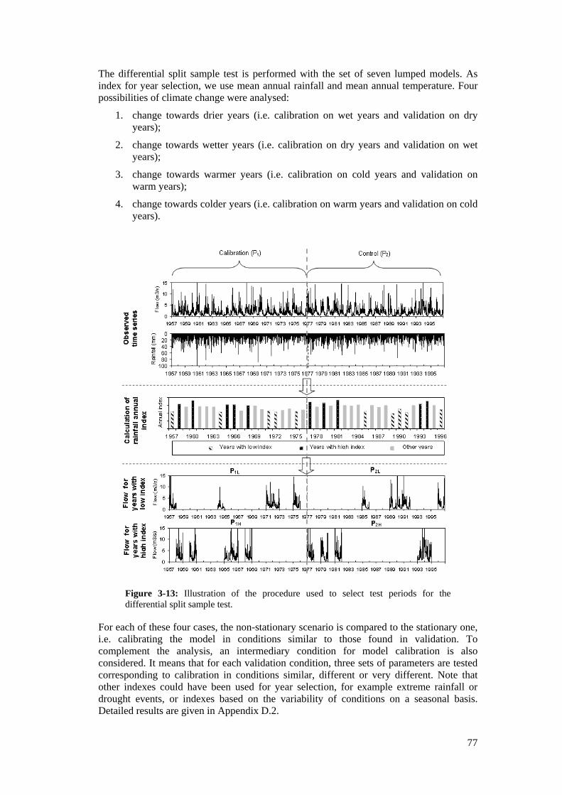
77
The differential split sample test is performed with the set of seven lumped models. As index for year selection, we use mean annual rainfall and mean annual temperature. Four possibilities of climate change were analysed:
1. change towards drier years (i.e. calibration on wet years and validation on dry years);
2. change towards wetter years (i.e. calibration on dry years and validation on wet years);
3. change towards warmer years (i.e. calibration on cold years and validation on warm years);
4. change towards colder years (i.e. calibration on warm years and validation on cold years).
Figure 3-13: Illustration of the procedure used to select test periods for the differential split sample test.
For each of these four cases, the non-stationary scenario is compared to the stationary one, i.e. calibrating the model in conditions similar to those found in validation. To complement the analysis, an intermediary condition for model calibration is also considered. It means that for each validation condition, three sets of parameters are tested corresponding to calibration in conditions similar, different or very different. Note that other indexes could have been used for year selection, for example extreme rainfall or drought events, or indexes based on the variability of conditions on a seasonal basis. Detailed results are given in Appendix D.2.
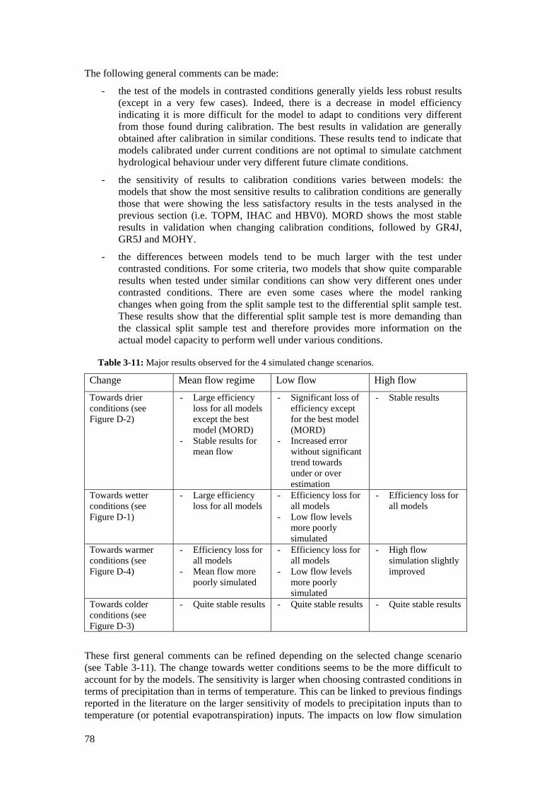
78
The following general comments can be made:
- the test of the models in contrasted conditions generally yields less robust results (except in a very few cases). Indeed, there is a decrease in model efficiency indicating it is more difficult for the model to adapt to conditions very different from those found during calibration. The best results in validation are generally obtained after calibration in similar conditions. These results tend to indicate that models calibrated under current conditions are not optimal to simulate catchment hydrological behaviour under very different future climate conditions.
- the sensitivity of results to calibration conditions varies between models: the models that show the most sensitive results to calibration conditions are generally those that were showing the less satisfactory results in the tests analysed in the previous section (i.e. TOPM, IHAC and HBV0). MORD shows the most stable results in validation when changing calibration conditions, followed by GR4J, GR5J and MOHY.
- the differences between models tend to be much larger with the test under contrasted conditions. For some criteria, two models that show quite comparable results when tested under similar conditions can show very different ones under contrasted conditions. There are even some cases where the model ranking changes when going from the split sample test to the differential split sample test. These results show that the differential split sample test is more demanding than the classical split sample test and therefore provides more information on the actual model capacity to perform well under various conditions.
Table 3-11: Major results observed for the 4 simulated change scenarios.
Change Mean flow regime Low flow High flow
Towards drier conditions (see Figure D-2)
- Large efficiency loss for all models except the best model (MORD)
- Stable results for mean flow
- Significant loss of efficiency except for the best model (MORD)
- Increased error without significant trend towards under or over estimation
- Stable results
Towards wetter conditions (see Figure D-1)
- Large efficiency loss for all models
- Efficiency loss for all models
- Low flow levels more poorly simulated
- Efficiency loss for all models
Towards warmer conditions (see Figure D-4)
- Efficiency loss for all models
- Mean flow more poorly simulated
- Efficiency loss for all models
- Low flow levels more poorly simulated
- High flow simulation slightly improved
Towards colder conditions (see Figure D-3)
- Quite stable results - Quite stable results - Quite stable results
These first general comments can be refined depending on the selected change scenario (see Table 3-11). The change towards wetter conditions seems to be the more difficult to account for by the models. The sensitivity is larger when choosing contrasted conditions in terms of precipitation than in terms of temperature. This can be linked to previous findings reported in the literature on the larger sensitivity of models to precipitation inputs than to temperature (or potential evapotranspiration) inputs. The impacts on low flow simulation
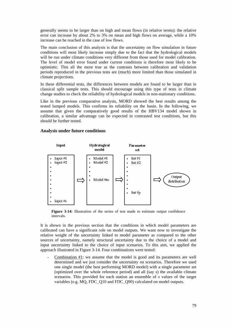
79
generally seems to be larger than on high and mean flows (in relative terms): the relative error can increase by about 2% to 3% on mean and high flows on average, while a 10% increase can be reached in the case of low flows.
The main conclusion of this analysis is that the uncertainty on flow simulation in future conditions will most likely increase simply due to the fact that the hydrological models will be run under climate conditions very different from those used for model calibration. The level of model error found under current conditions is therefore most likely to be optimistic. This all the more true as the contrasts between calibration and validation periods reproduced in the previous tests are (much) more limited than those simulated in climate projections.
In these differential tests, the differences between models are found to be larger than in classical split sample tests. This should encourage using this type of tests in climate change studies to check the reliability of hydrological models in non-stationary conditions.
Like in the previous comparative analysis, MORD showed the best results among the tested lumped models. This confirms its reliability on the basin. In the following, we assume that given the comparatively good results of the HBV134 model shown in calibration, a similar advantage can be expected in contrasted test conditions, but this should be further tested.
Analysis under future conditions
Figure 3-14: Illustration of the series of test made to estimate output confidence intervals.
It is shown in the previous section that the conditions in which model parameters are calibrated can have a significant role on model outputs. We want now to investigate the relative weight of the uncertainty linked to model parameter as compared to the other sources of uncertainty, namely structural uncertainty due to the choice of a model and input uncertainty linked to the choice of input scenarios. To this aim, we applied the approach illustrated in Figure 3-14. Four combinations were tested:
- Combination #1: we assume that the model is good and its parameters are well determined and we just consider the uncertainty on scenarios. Therefore we used one single model (the best performing MORD model) with a single parameter set (optimized over the whole reference period) and all (say s) the available climate scenarios. This provided for each station an ensemble of s values of the target variables (e.g. MQ, FDC_Q10 and FDC_Q90) calculated on model outputs.
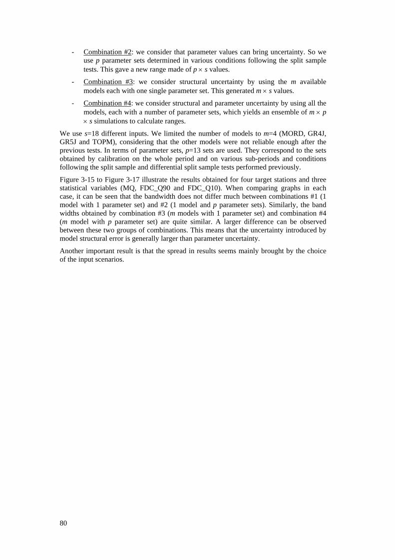
80
- Combination #2: we consider that parameter values can bring uncertainty. So we use p parameter sets determined in various conditions following the split sample tests. This gave a new range made of p × s values.
- Combination #3: we consider structural uncertainty by using the m available models each with one single parameter set. This generated m × s values.
- Combination #4: we consider structural and parameter uncertainty by using all the models, each with a number of parameter sets, which yields an ensemble of m × p × s simulations to calculate ranges.
We use s=18 different inputs. We limited the number of models to m=4 (MORD, GR4J, GR5J and TOPM), considering that the other models were not reliable enough after the previous tests. In terms of parameter sets, p=13 sets are used. They correspond to the sets obtained by calibration on the whole period and on various sub-periods and conditions following the split sample and differential split sample tests performed previously.
Figure 3-15 to Figure 3-17 illustrate the results obtained for four target stations and three statistical variables (MQ, FDC_Q90 and FDC_Q10). When comparing graphs in each case, it can be seen that the bandwidth does not differ much between combinations #1 (1 model with 1 parameter set) and #2 (1 model and p parameter sets). Similarly, the band widths obtained by combination #3 (m models with 1 parameter set) and combination #4 (m model with p parameter set) are quite similar. A larger difference can be observed between these two groups of combinations. This means that the uncertainty introduced by model structural error is generally larger than parameter uncertainty.
Another important result is that the spread in results seems mainly brought by the choice of the input scenarios.
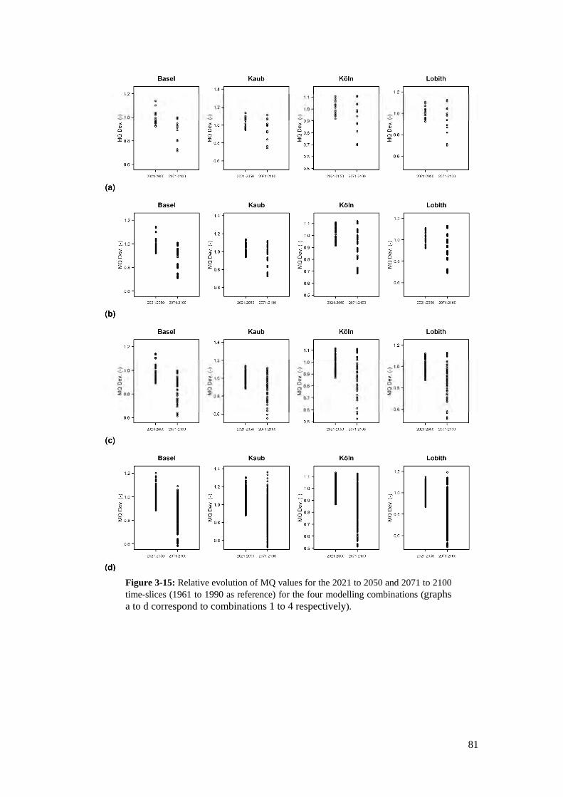
81
Figure 3-15: Relative evolution of MQ values for the 2021 to 2050 and 2071 to 2100 time-slices (1961 to 1990 as reference) for the four modelling combinations (graphs a to d correspond to combinations 1 to 4 respectively).
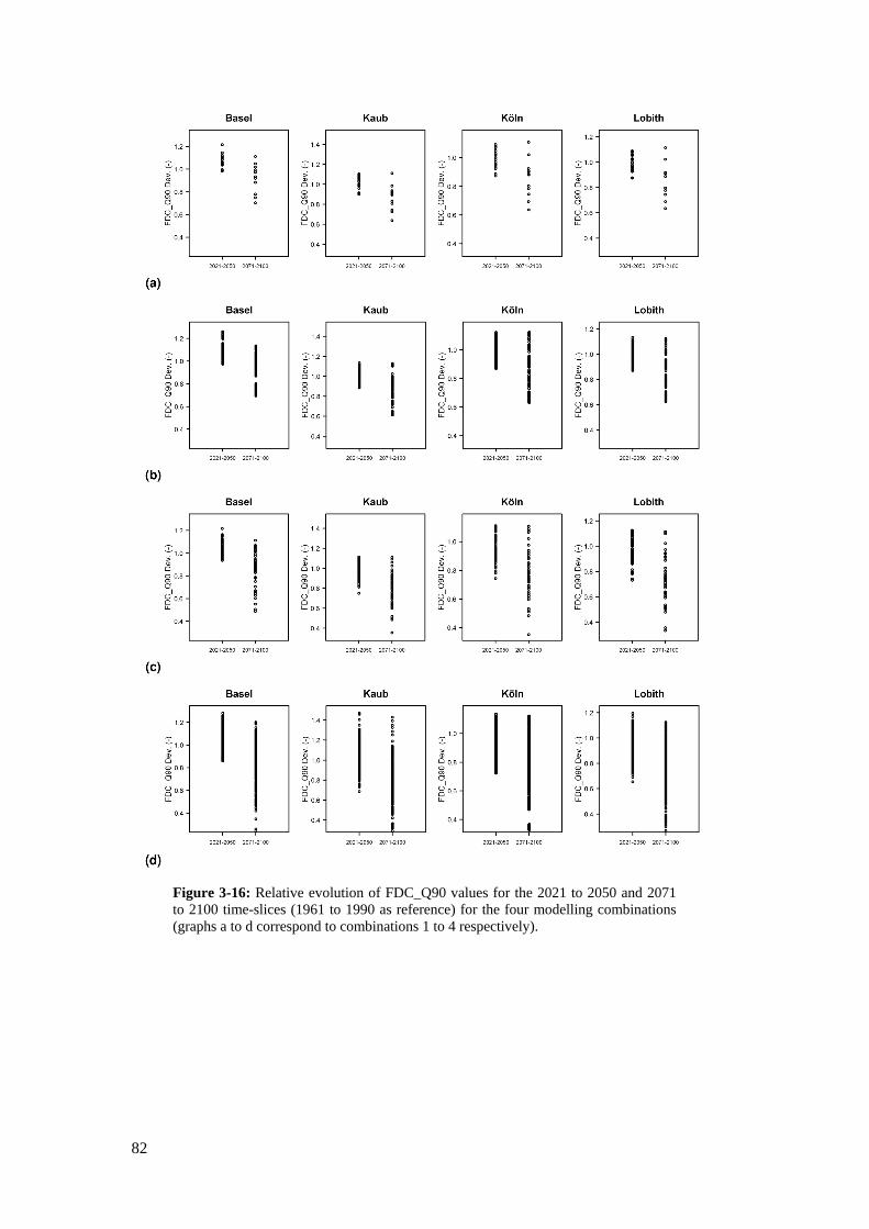
82
Figure 3-16: Relative evolution of FDC_Q90 values for the 2021 to 2050 and 2071 to 2100 time-slices (1961 to 1990 as reference) for the four modelling combinations (graphs a to d correspond to combinations 1 to 4 respectively).
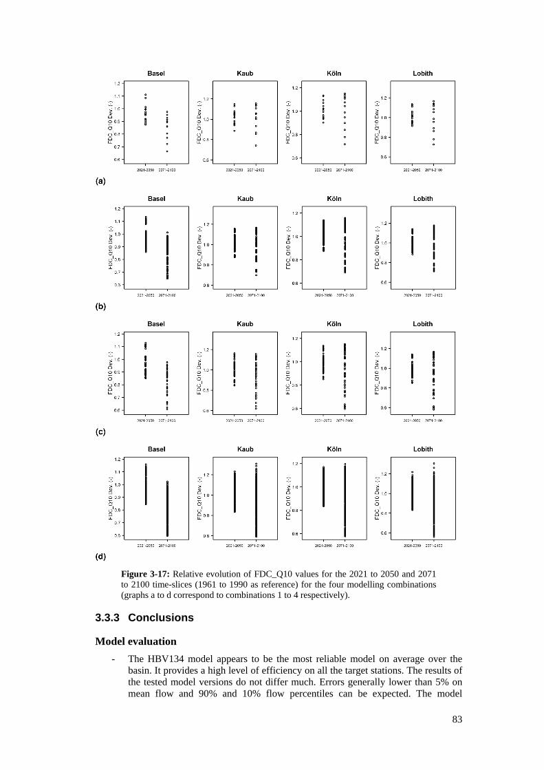
83
Figure 3-17: Relative evolution of FDC_Q10 values for the 2021 to 2050 and 2071 to 2100 time-slices (1961 to 1990 as reference) for the four modelling combinations (graphs a to d correspond to combinations 1 to 4 respectively).
3.3.3 Conclusions
Model evaluation - The HBV134 model appears to be the most reliable model on average over the
basin. It provides a high level of efficiency on all the target stations. The results of the tested model versions do not differ much. Errors generally lower than 5% on mean flow and 90% and 10% flow percentiles can be expected. The model
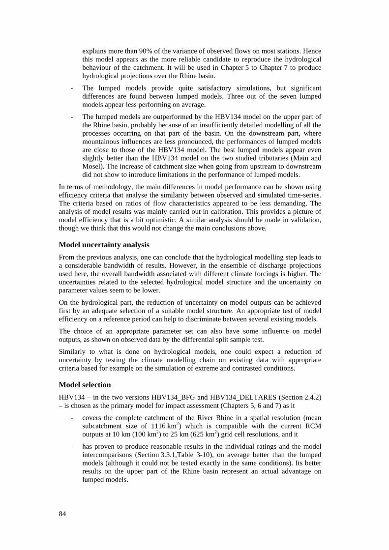
84
explains more than 90% of the variance of observed flows on most stations. Hence this model appears as the more reliable candidate to reproduce the hydrological behaviour of the catchment. It will be used in Chapter 5 to Chapter 7 to produce hydrological projections over the Rhine basin.
- The lumped models provide quite satisfactory simulations, but significant differences are found between lumped models. Three out of the seven lumped models appear less performing on average.
- The lumped models are outperformed by the HBV134 model on the upper part of the Rhine basin, probably because of an insufficiently detailed modelling of all the processes occurring on that part of the basin. On the downstream part, where mountainous influences are less pronounced, the performances of lumped models are close to those of the HBV134 model. The best lumped models appear even slightly better than the HBV134 model on the two studied tributaries (Main and Mosel). The increase of catchment size when going from upstream to downstream did not show to introduce limitations in the performance of lumped models.
In terms of methodology, the main differences in model performance can be shown using efficiency criteria that analyse the similarity between observed and simulated time-series. The criteria based on ratios of flow characteristics appeared to be less demanding. The analysis of model results was mainly carried out in calibration. This provides a picture of model efficiency that is a bit optimistic. A similar analysis should be made in validation, though we think that this would not change the main conclusions above.
Model uncertainty analysis From the previous analysis, one can conclude that the hydrological modelling step leads to a considerable bandwidth of results. However, in the ensemble of discharge projections used here, the overall bandwidth associated with different climate forcings is higher. The uncertainties related to the selected hydrological model structure and the uncertainty on parameter values seem to be lower.
On the hydrological part, the reduction of uncertainty on model outputs can be achieved first by an adequate selection of a suitable model structure. An appropriate test of model efficiency on a reference period can help to discriminate between several existing models.
The choice of an appropriate parameter set can also have some influence on model outputs, as shown on observed data by the differential split sample test.
Similarly to what is done on hydrological models, one could expect a reduction of uncertainty by testing the climate modelling chain on existing data with appropriate criteria based for example on the simulation of extreme and contrasted conditions.
Model selection HBV134 – in the two versions HBV134_BFG and HBV134_DELTARES (Section 2.4.2) – is chosen as the primary model for impact assessment (Chapters 5, 6 and 7) as it
- covers the complete catchment of the River Rhine in a spatial resolution (mean subcatchment size of 1116 km2) which is compatible with the current RCM outputs at 10 km (100 km2) to 25 km (625 km2) grid cell resolutions, and it
- has proven to produce reasonable results in the individual ratings and the model intercomparisons (Section 3.3.1,Table 3-10), on average better than the lumped models (although it could not be tested exactly in the same conditions). Its better results on the upper part of the Rhine basin represent an actual advantage on lumped models.
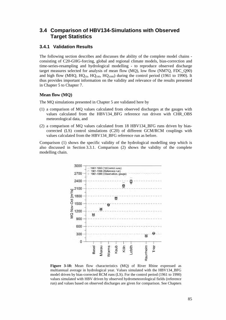
85
3.4 Comparison of HBV134-Simulations with Observed Target Statistics
3.4.1 Validation Results
The following section describes and discusses the ability of the complete model chains - consisting of C20-GHG-forcing, global and regional climate models, bias-correction and time-series-resampling and hydrological modelling - to reproduce observed discharge target measures selected for analysis of mean flow (MQ), low flow (NM7Q, FDC_Q90) and high flow (MHQ, HQ10, HQ100, HQ1000) during the control period (1961 to 1990). It thus provides important information on the validity and relevance of the results presented in Chapter 5 to Chapter 7.
Mean flow (MQ) The MQ simulations presented in Chapter 5 are validated here by
(1) a comparison of MQ values calculated from observed discharges at the gauges with values calculated from the HBV134_BFG reference run driven with CHR_OBS meteorological data, and
(2) a comparison of MQ values calculated from 18 HBV134_BFG runs driven by bias-corrected (LS) control simulations (C20) of different GCM/RCM couplings with values calculated from the HBV134_BFG reference run as before.
Comparison (1) shows the specific validity of the hydrological modelling step which is also discussed in Section 3.3.1. Comparison (2) shows the validity of the complete modelling chain.
Figure 3-18: Mean flow characteristics (MQ) of River Rhine expressed as multiannual average in hydrological year. Values simulated with the HBV134_BFG model driven by bias-corrected RCM runs (LS). For the control period (1961 to 1990) values simulated with HBV driven by observed hydrometeorological fields (reference run) and values based on observed discharges are given for comparison. See Chapters
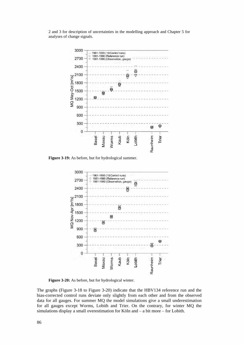
86
2 and 3 for description of uncertainties in the modelling approach and Chapter 5 for analyses of change signals.
Figure 3-19: As before, but for hydrological summer.
Figure 3-20: As before, but for hydrological winter.
The graphs (Figure 3-18 to Figure 3-20) indicate that the HBV134 reference run and the bias-corrected control runs deviate only slightly from each other and from the observed data for all gauges. For summer MQ the model simulations give a small underestimation for all gauges except Worms, Lobith and Trier. On the contrary, for winter MQ the simulations display a small overestimation for Köln and – a bit more – for Lobith.
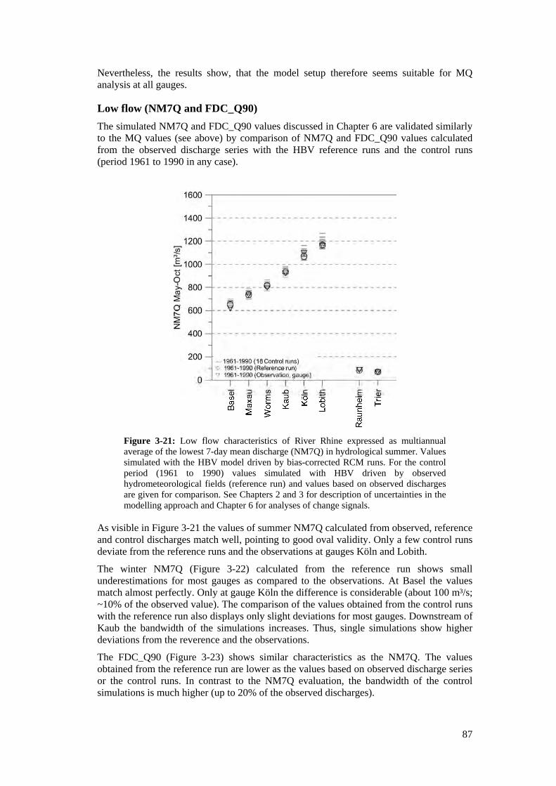
87
Nevertheless, the results show, that the model setup therefore seems suitable for MQ analysis at all gauges.
Low flow (NM7Q and FDC_Q90) The simulated NM7Q and FDC_Q90 values discussed in Chapter 6 are validated similarly to the MQ values (see above) by comparison of NM7Q and FDC_Q90 values calculated from the observed discharge series with the HBV reference runs and the control runs (period 1961 to 1990 in any case).
Figure 3-21: Low flow characteristics of River Rhine expressed as multiannual average of the lowest 7-day mean discharge (NM7Q) in hydrological summer. Values simulated with the HBV model driven by bias-corrected RCM runs. For the control period (1961 to 1990) values simulated with HBV driven by observed hydrometeorological fields (reference run) and values based on observed discharges are given for comparison. See Chapters 2 and 3 for description of uncertainties in the modelling approach and Chapter 6 for analyses of change signals.
As visible in Figure 3-21 the values of summer NM7Q calculated from observed, reference and control discharges match well, pointing to good oval validity. Only a few control runs deviate from the reference runs and the observations at gauges Köln and Lobith.
The winter NM7Q (Figure 3-22) calculated from the reference run shows small underestimations for most gauges as compared to the observations. At Basel the values match almost perfectly. Only at gauge Köln the difference is considerable (about 100 m³/s; ~10% of the observed value). The comparison of the values obtained from the control runs with the reference run also displays only slight deviations for most gauges. Downstream of Kaub the bandwidth of the simulations increases. Thus, single simulations show higher deviations from the reverence and the observations.
The FDC_Q90 (Figure 3-23) shows similar characteristics as the NM7Q. The values obtained from the reference run are lower as the values based on observed discharge series or the control runs. In contrast to the NM7Q evaluation, the bandwidth of the control simulations is much higher (up to 20% of the observed discharges).
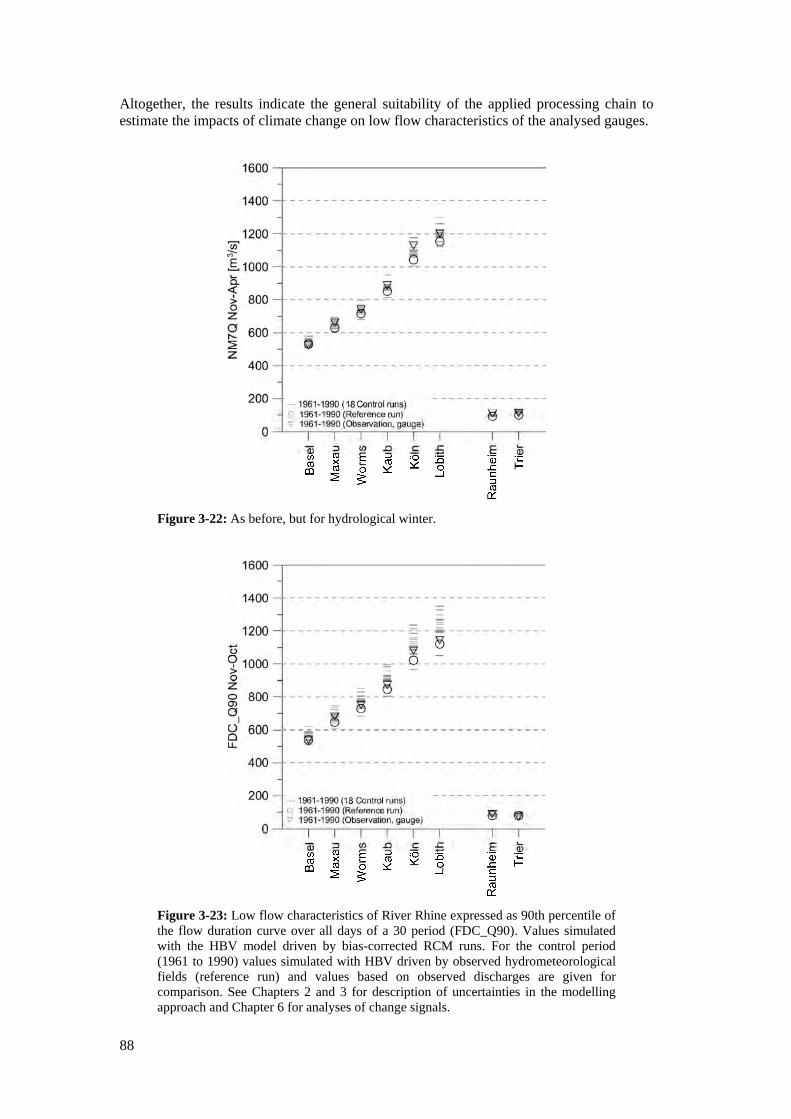
88
Altogether, the results indicate the general suitability of the applied processing chain to estimate the impacts of climate change on low flow characteristics of the analysed gauges.
Figure 3-22: As before, but for hydrological winter.
Figure 3-23: Low flow characteristics of River Rhine expressed as 90th percentile of the flow duration curve over all days of a 30 period (FDC_Q90). Values simulated with the HBV model driven by bias-corrected RCM runs. For the control period (1961 to 1990) values simulated with HBV driven by observed hydrometeorological fields (reference run) and values based on observed discharges are given for comparison. See Chapters 2 and 3 for description of uncertainties in the modelling approach and Chapter 6 for analyses of change signals.
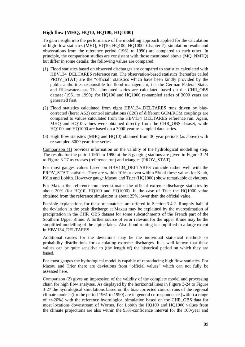
89
High flow (MHQ, HQ10, HQ100, HQ1000) To gain insight into the performance of the modelling approach applied for the calculation of high flow statistics (MHQ, HQ10, HQ100, HQ1000; Chapter 7), simulation results and observations from the reference period (1961 to 1990) are compared to each other. In principle, the comparison studies are consistent with those mentioned above (MQ, NM7Q) but differ in some details; the following values are compared:
(1) Flood statistics based on observed discharges are compared to statistics calculated with HBV134_DELTARES reference run. The observation-based statistics (hereafter called PROV_STAT) are the “official” statistics which have been kindly provided by the public authorities responsible for flood management; i.e. the German Federal States and Rijkswaterstaat. The simulated series are calculated based on the CHR_OBS dataset (1961 to 1990); for HQ100 and HQ1000 re-sampled series of 3000 years are generated first.
(2) Flood statistics calculated from eight HBV134_DELTARES runs driven by bias-corrected (here: AS2) control simulations (C20) of different GCM/RCM couplings are compared to values calculated from the HBV134_DELTARES reference run. Again, MHQ and HQ10 values were obtained directly from the CHR_OBS dataset, while HQ100 and HQ1000 are based on a 3000-year re-sampled data series.
(3) High flow statistics (MHQ and HQ10) obtained from 30 year periods (as above) with re-sampled 3000 year time-series.
Comparison (1) provides information on the validity of the hydrological modelling step. The results for the period 1961 to 1990 at the 8 gauging stations are given in Figure 3-24 to Figure 3-27 as crosses (reference run) and triangles (PROV_STAT).
For most gauges values based on HBV134_DELTARES coincide rather well with the PROV_STAT statistics. They are within 10% or even within 5% of these values for Kaub, Köln and Lobith. However gauge Maxau and Trier (HQ1000) show remarkable deviations.
For Maxau the reference run overestimates the official extreme discharge statistics by about 20% (for HQ10, HQ100 and HQ1000). In the case of Trier the HQ1000 value obtained from the reference simulation is about 25% lower than the official value.
Possible explanations for these mismatches are offered in Section 3.4.2. Roughly half of the deviation in the peak discharge at Maxau may be explained by the overestimation of precipitation in the CHR_OBS dataset for some subcatchments of the French part of the Southern Upper Rhine. A further source of error relevant for the upper Rhine may be the simplified modelling of the alpine lakes. Also flood routing is simplified to a large extent in HBV134_DELTARES.
Additional causes for the deviations may be the individual statistical methods or probability distributions for calculating extreme discharges. It is well known that these values can be quite sensitive to (the length of) the historical period on which they are based.
For most gauges the hydrological model is capable of reproducing high flow statistics. For Maxau and Trier there are deviations from “official values” which can not fully be assessed here.
Comparison (2) gives an impression of the validity of the complete model and processing chain for high flow analyses. As displayed by the horizontal lines in Figure 3-24 to Figure 3-27 the hydrological simulations based on the bias-corrected control runs of the regional climate models (for the period 1961 to 1990) are in general correspondence (within a range of +/-20%) with the reference hydrological simulation based on the CHR_OBS data for most locations downstream of Worms. For Lobith the HQ100 and HQ1000 values from the climate projections are also within the 95%-confidence interval for the 100-year and
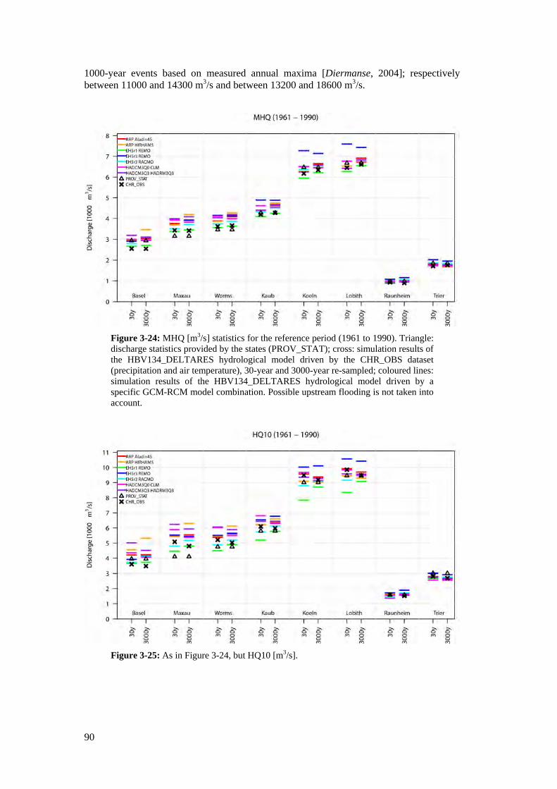
90
1000-year events based on measured annual maxima [Diermanse, 2004]; respectively between 11000 and 14300 m3/s and between 13200 and 18600 m3/s.
Figure 3-24: MHQ [m3/s] statistics for the reference period (1961 to 1990). Triangle: discharge statistics provided by the states (PROV_STAT); cross: simulation results of the HBV134_DELTARES hydrological model driven by the CHR_OBS dataset (precipitation and air temperature), 30-year and 3000-year re-sampled; coloured lines: simulation results of the HBV134_DELTARES hydrological model driven by a specific GCM-RCM model combination. Possible upstream flooding is not taken into account.
Figure 3-25: As in Figure 3-24, but HQ10 [m3/s].
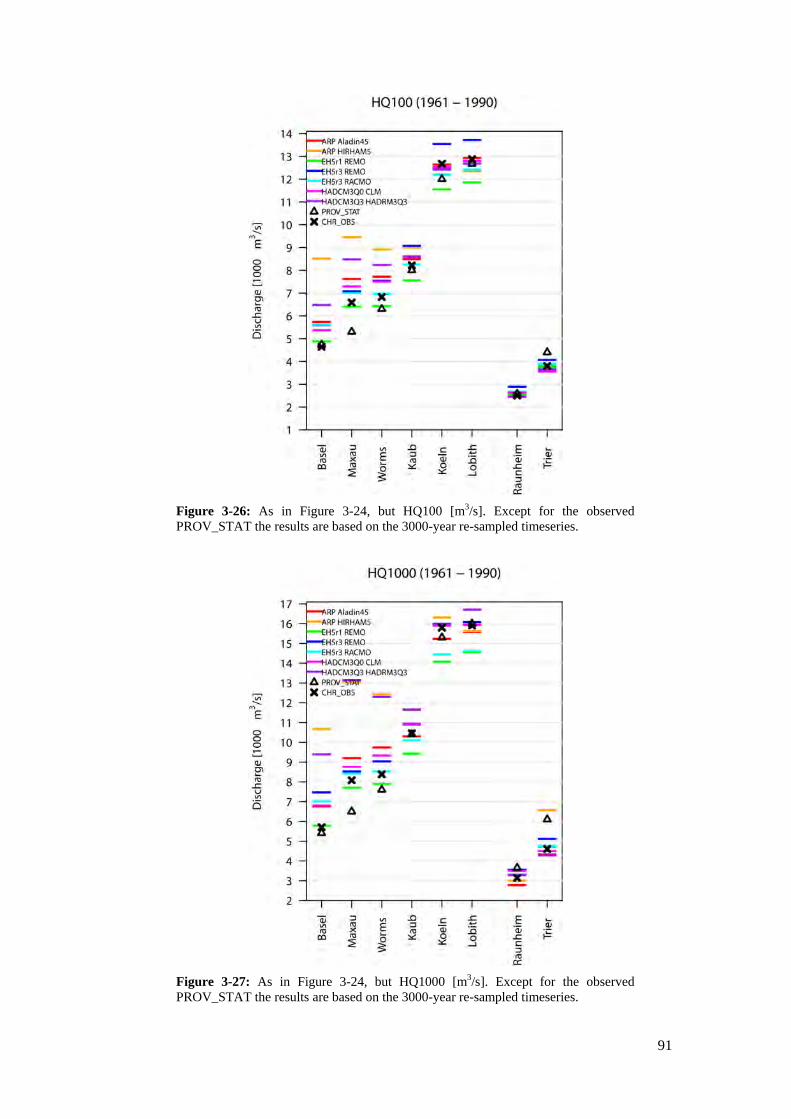
91
Figure 3-26: As in Figure 3-24, but HQ100 [m3/s]. Except for the observed PROV_STAT the results are based on the 3000-year re-sampled timeseries.
Figure 3-27: As in Figure 3-24, but HQ1000 [m3/s]. Except for the observed PROV_STAT the results are based on the 3000-year re-sampled timeseries.
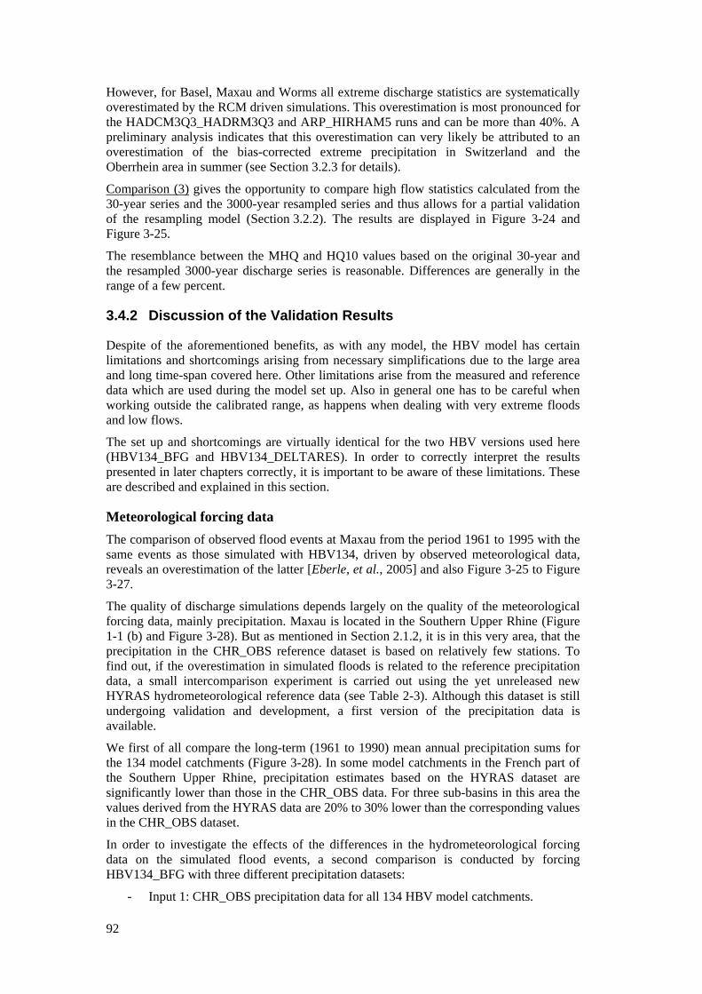
92
However, for Basel, Maxau and Worms all extreme discharge statistics are systematically overestimated by the RCM driven simulations. This overestimation is most pronounced for the HADCM3Q3_HADRM3Q3 and ARP_HIRHAM5 runs and can be more than 40%. A preliminary analysis indicates that this overestimation can very likely be attributed to an overestimation of the bias-corrected extreme precipitation in Switzerland and the Oberrhein area in summer (see Section 3.2.3 for details).
Comparison (3) gives the opportunity to compare high flow statistics calculated from the 30-year series and the 3000-year resampled series and thus allows for a partial validation of the resampling model (Section 3.2.2). The results are displayed in Figure 3-24 and Figure 3-25.
The resemblance between the MHQ and HQ10 values based on the original 30-year and the resampled 3000-year discharge series is reasonable. Differences are generally in the range of a few percent.
3.4.2 Discussion of the Validation Results
Despite of the aforementioned benefits, as with any model, the HBV model has certain limitations and shortcomings arising from necessary simplifications due to the large area and long time-span covered here. Other limitations arise from the measured and reference data which are used during the model set up. Also in general one has to be careful when working outside the calibrated range, as happens when dealing with very extreme floods and low flows.
The set up and shortcomings are virtually identical for the two HBV versions used here (HBV134_BFG and HBV134_DELTARES). In order to correctly interpret the results presented in later chapters correctly, it is important to be aware of these limitations. These are described and explained in this section.
Meteorological forcing data The comparison of observed flood events at Maxau from the period 1961 to 1995 with the same events as those simulated with HBV134, driven by observed meteorological data, reveals an overestimation of the latter [Eberle, et al., 2005] and also Figure 3-25 to Figure 3-27.
The quality of discharge simulations depends largely on the quality of the meteorological forcing data, mainly precipitation. Maxau is located in the Southern Upper Rhine (Figure 1-1 (b) and Figure 3-28). But as mentioned in Section 2.1.2, it is in this very area, that the precipitation in the CHR_OBS reference dataset is based on relatively few stations. To find out, if the overestimation in simulated floods is related to the reference precipitation data, a small intercomparison experiment is carried out using the yet unreleased new HYRAS hydrometeorological reference data (see Table 2-3). Although this dataset is still undergoing validation and development, a first version of the precipitation data is available.
We first of all compare the long-term (1961 to 1990) mean annual precipitation sums for the 134 model catchments (Figure 3-28). In some model catchments in the French part of the Southern Upper Rhine, precipitation estimates based on the HYRAS dataset are significantly lower than those in the CHR_OBS data. For three sub-basins in this area the values derived from the HYRAS data are 20% to 30% lower than the corresponding values in the CHR_OBS dataset.
In order to investigate the effects of the differences in the hydrometeorological forcing data on the simulated flood events, a second comparison is conducted by forcing HBV134_BFG with three different precipitation datasets:
- Input 1: CHR_OBS precipitation data for all 134 HBV model catchments.
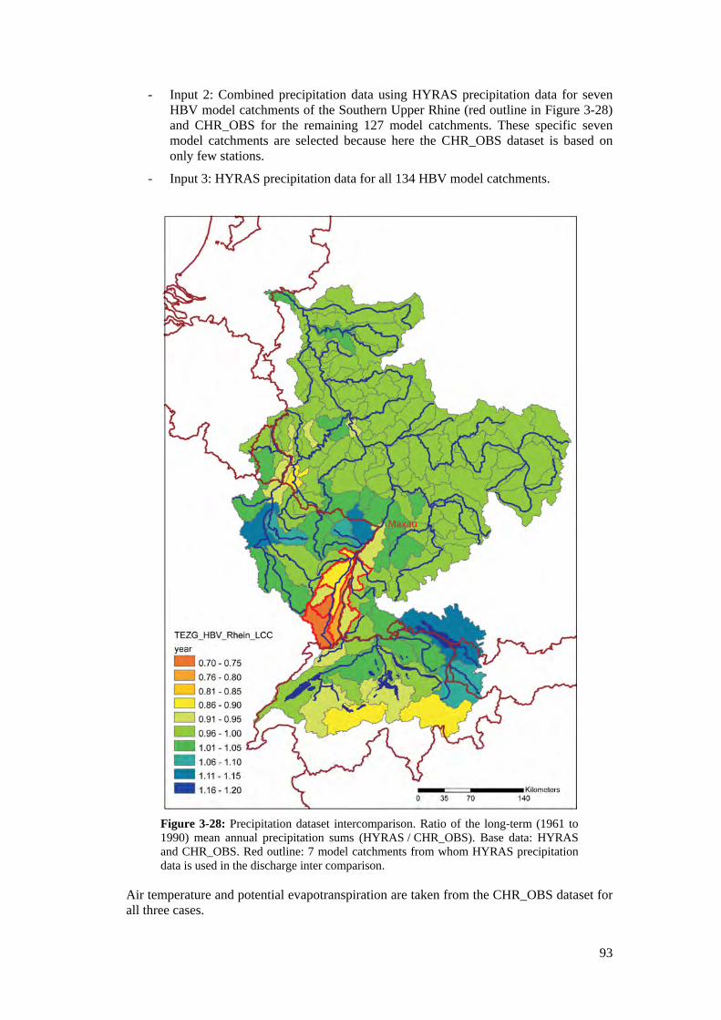
93
- Input 2: Combined precipitation data using HYRAS precipitation data for seven HBV model catchments of the Southern Upper Rhine (red outline in Figure 3-28) and CHR_OBS for the remaining 127 model catchments. These specific seven model catchments are selected because here the CHR_OBS dataset is based on only few stations.
- Input 3: HYRAS precipitation data for all 134 HBV model catchments.
Figure 3-28: Precipitation dataset intercomparison. Ratio of the long-term (1961 to 1990) mean annual precipitation sums (HYRAS / CHR_OBS). Base data: HYRAS and CHR_OBS. Red outline: 7 model catchments from whom HYRAS precipitation data is used in the discharge inter comparison.
Air temperature and potential evapotranspiration are taken from the CHR_OBS dataset for all three cases.
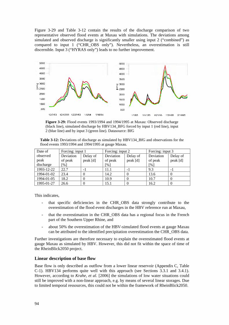
94
Figure 3-29 and Table 3-12 contain the results of the discharge comparison of two representative observed flood events at Maxau with simulations. The deviations among simulated and observed discharge is significantly smaller using input 2 (“combined”) as compared to input 1 (“CHR_OBS only”). Nevertheless, an overestimation is still discernible. Input 3 (“HYRAS only”) leads to no further improvement.
Figure 3-29: Flood events 1993/1994 and 1994/1995 at Maxau: Observed discharge (black line), simulated discharge by HBV134_BFG forced by input 1 (red line), input 2 (blue line) and by input 3 (green line). Datasource: BfG
Table 3-12: Deviations of discharge as simulated by HBV134_BfG and observations for the flood events 1993/1994 and 1994/1995 at gauge Maxau.
Date of observed peak discharge
Forcing: input 1 Forcing: input 2 Forcing: input 3 Deviation of peak [%]
Delay of peak [d]
Deviation of peak [%]
Delay of peak [d]
Deviation of peak [%]
Delay of peak [d]
1993-12-22 22.7 -1 11.1 -1 9.3 -1 1994-01-02 23.4 0 14.2 0 13.6 0 1994-01-05 18.2 0 10.9 0 10.7 0 1995-01-27 26.6 0 15.1 0 16.2 0
This indicates,
- that specific deficiencies in the CHR_OBS data strongly contribute to the overestimation of the flood event discharges in the HBV reference run at Maxau,
- that the overestimation in the CHR_OBS data has a regional focus in the French part of the Southern Upper Rhine, and
- about 50% the overestimation of the HBV-simulated flood events at gauge Maxau can be attributed to the identified precipitation overestimation the CHR_OBS data.
Further investigations are therefore necessary to explain the overestimated flood events at gauge Maxau as simulated by HBV. However, this did not fit within the space of time of the RheinBlick2050 project.
Linear description of base flow Base flow is only described as outflow from a lower linear reservoir (Appendix C, Table C-1). HBV134 performs quite well with this approach (see Sections 3.3.1 and 3.4.1). However, according to Krahe, et al. [2006] the simulations of low water situations could still be improved with a non-linear approach, e.g. by means of several linear storages. Due to limited temporal ressources, this could not be within the framework of RheinBlick2050.
95
Lakes In order to keep the model structure simple, lakes are not simulated explicitly. The impact of large lakes like Lake Constance, Lake Biel and other Swiss lakes on floods is only approximated by using the routing method implemented in the HBV (Appendix C). A full lake retention approach is not implemented yet.
This has to be taken into account when interpreting the results mainly for the upper Rhine River gauging stations Basel, Maxau and Worms. On the other hand the calibration result in terms of the Nash-Sutcliffe Criterion for Basel is not worse than for other locations [Eberle, et al., 2005]. The results above also show that for floods the performance of the model is good for Basel, indicating that results are not too sensitive to the modelling of the large lakes.
Flood routing No hydraulic models are used. Just the simple internal flood routing from the hydrological model (HBV) is used for the routing of the main branch of the Rhine River. Hydraulic effects are therefore simplified to a high extent, not really taking into account the damping of extreme discharges due e.g. to overtopping of dikes. At gauging stations downstream of areas, that possibly would be flooded, this may lead to simulated (peak-)discharges, which are higher than they would actually be observed in reality7.
Downstream from gauge Maxau, an artificial loss of water during flood events is implemented in the HBV134 model. This correction is intended to compensate the backwater effect8, which occurs where tributary rivers enter the main stream. It might also compensate partly for the effect of erroneous precipitation data (see above) used for the calibration in the French part of the Southern Upper Rhine.
Only the combination of hydrological with hydraulic modelling would lead to more realistic simulation results, but the additional hydraulic simulations are computationally very expensive as well (especially since many thousands of years are involved; Section 3.2.2) and did not fit in the time-schedule of the RheinBlick2050 project.
Though the simplification of flood routing introduces some additional uncertainties, it only affects the extreme discharge (HQx) simulations and analyses in Chapter 7. Other quantities like average discharge and low flow are not affected (Chapter 5 and Chapter 6).
3.4.3 Conclusions
In this section we describe the ability of (1) the hydrological model i.e. HBV134 forced by CHR_OBS and (2) the complete model chain – consisting of C20-GHG-forcing, global and regional climate models, bias-correction (and time-series-resampling) forcing HBV134 – to produce reliable discharge results during the control period (1961 to 1990).
7 This limitation is not specific to the model chain used in this project. The detailled effects of flooding are also not fully considered in the “official” statistics, since the observed flow data used to calculate these statistics do not include days when upstream flooding took place. The design discharges for the dikes along the Rhine River given in Appendix G may give an indication above which discharge values flooding may occur. The hydraulic system along the Rhine however is very complex in a way that one cannot define a specific discharge for each gauge above which flooding has taken place further upstream. 8 Backwater effect is defined as the rise in elevation of the surface profile of a stream when the flow is retarded above a dam or any other obstruction or is backed-up into a tributary by a flood in the main stream.
96
For most target measures, the suitability of the HBV134 model and the model/processing chain can be confirmed. We have the highest confidence in the simulated MQ values. As expected, extreme discharge statistics are surrounded with larger uncertainties.
Observed NM7Q low flow statistics are matched well by HBV134 and the full model chain, although the scatter of results of different model combinations is wider as compared to mean flow (MQ). The HBV reference run reproduces well the FDC_Q90 statistic at all gauges. However, the complete model chain produces a systematic overestimation increasing up to gauge Lobith. We expect that this characteristic will not have a large effect when considering the difference of a future period and the control period. However, this has to be further investigated.
Regarding the simulation of high flows we can distinguish two regimes; gauges where high flows occur predominantly in winter (Lobith, Köln, Kaub, Raunheim and Trier) and those where high flows are mostly summer related (Basel, Maxau and Worms). In general the performance of the model chain is considerably better for gauges with winter high flows.
For gauges Kaub, Köln and Lobith the performance is comparable and satisfactory for MHQ, HQ10, HQ100 and HQ1000. This holds for the HBV model forced with the CHR_OBS data (the HBV reference run) as well as for the HBV model forced with the bias-corrected RCM control (1961 to 1990) runs.
For gauges Basel, Maxau and Worms the performance of the model chain is less satisfactory. For Maxau HQ10, HQ100 and HQ1000 are considerably overestimated by the HBV134 reference run which at least can be partly related to the overestimation of precipitation in the French part of the Southern Upper Rhine in the CHR_OBS data. This problem also seems to affect the simulated high flow statistics at Worms.
In addition, at Basel, Maxau and Worms, for all high flow statistics the HBV simulations driven by the bias-corrected RCM control runs systematically overestimate the HBV reference results. This latter problem is due to the overestimation (i.e. overcorrection) of extreme 10-day precipitation amounts in the hydrological summer in Switzerland and the Oberrhein area in the bias-correction method (AS2) chosen for the high flow analysis. Alternative bias-corrections methods are available that do not suffer from this particular problem but they are not used because of another imperfection. There is no time to solve these bias-correction problems satisfactorily within the RheinBlick2050 project. It is therefore decided not to give interpretations on future high flow projections for Basel, Maxau and Worms.
HQ100 and HQ1000 projections are based on rainfall generator re-sampled precipitation and temperature series of 3000 years. For MHQ and HQ10 it is shown that the results with 3000-year re-sampled series correspond well to the results with the not re-sampled 30-year series.
3.5 Overall Conclusions of the Validation
In this chapter we evaluate 37 regional climate simulations9, 8 hydrological models, 4 bias-correction methods and one time-series resampling approach for their suitability for the purpose of this study, i.e. the assessment of climate change (mean air temperature and precipitation) and discharge change (in terms of mean, high and low flow).
Based on the evaluation, a set of 20 regional climate projections10 (for far future 17 projections)11 is regarded as suitable (Section 3.1) to be used as input for hydrological
9 based on 22 different couplings of emission scenarios, global and regional climate models 10 based on 16 different couplings of emission scenarios, global and regional climate models 11 based on 13 different couplings of emission scenarios, global and regional climate models
97
modelling of the river Rhine assessment. This ensemble forms the basis for the climate change analyses and the hydrological impact assessment. The high flow analysis (Chapter 7) is based on a smaller ensemble of 7 projections12 (for far future 6 projections13), as the data processing chain is more complex.
The processing steps evaluated here (bias-correction, time-series resampling) yield satisfying results for most simulation targets (Section 3.2). With respect to bias-correction, a simple linear bias-correction approach (LS) already shows to work good for mean and low flow statistics. For high flow a non-linear scaling correction approach (AS2) and a time-series resampling approach is applied to better resolve extreme precipitation events and their return periods. The AS2 bias-correction method shows to produce valid results for the winter half year. However, it systematically overestimates (i.e. overcorrects) extreme precipitation amounts in the hydrological summer in Switzerland and the Oberrhein area leading to a systematic overestimation of high flow statistics at Basel, Maxau and Worms. Two alternative non-linear bias-correction approaches which do not have this particular problem are not chosen because of another imperfection. There is no time to solve these bias-correction problems satisfactorily within the RheinBlick2050 project and it is decided that no high flow projections are presented for Basel, Maxau and Worms.
The comparison of different hydrological model structures and parameter sets shows that the hydrological modelling step alone leads to a considerable bandwidth of results. However in the ensemble of discharge projections used here, the overall bandwidth associated with different climate forcings is larger (Section 3.3).
In the model comparison the semi-distributed hydrological model HBV134 gives better results than the lumped models on average on the eight target gauging stations. Also with respect to the hydrological target measures chosen in this study, the suitability of HBV134 can be confirmed (Section 3.4). Therefore, HBV134 is chosen as the main tool for the hydrological analyses.
Finally, we evaluate the ability of the complete model chains and processing procedures14 to reproduce the target discharge measures during the control period (1961 to 1990). We have the highest confidence in the simulated mean flow statistics (MQ). As expected, extreme discharge statistics show higher uncertainties. The simulated low flow statistics values (NM7Q, FDC_Q90) are reasonably reproduced.
Regarding the simulation of high flows the performance of the model chain is considerably better for gauges with winter high flows (Lobith, Köln, Kaub, Raunheim and Trier) than for gauges where high flows occur mostly in summer (Basel, Maxau and Worms). For the latter gauges it is therefore decided not to give interpretations on future high flow projections for Basel, Maxau and Worms.
In summary, the evaluation procedure applied here, leads to a selection of model chains and processing procedures, which are regarded as suitable to derive discharge projections for the future climate except for high flow statistics at Basel, Maxau and Worms. This well defined ensemble is a prerequisite for the construction of “robust” scenarios of future climate and discharge conditions in the Rhine River basin. The “robustness” of a scenario, as we propose here, includes two aspects: (1) careful evaluation of all model chains and processing procedures, and (2) incorporation of the overall uncertainty in the presentation of results.
12 based on 6 different couplings of emission scenarios, global and regional climate models 13 based on 5 different couplings of emission scenarios, global and regional climate models 14 Consisting of GHG-forcing, global and regional climate models, bias correction (time-series resampling) and hydrological model. For MQ, NM7Q and FDC_Q90 we evaluated 18 simulations based on 13 different couplings; for MHQ, HQ10, HQ100 and HQ1000 we used 7 simulations based on 6 different couplings.

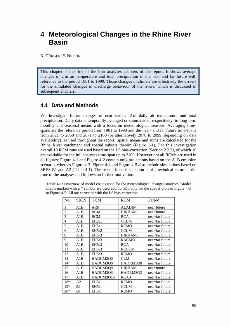
99
4 Meteorological Changes in the Rhine River Basin
K. GÖRGEN, E. NILSON
This chapter is the first of the four analyses chapters of the report. It shows average changes of 2 m air temperature and total precipitation in the near and far future with reference to the period 1961 to 1990. Those changes in climate are effectively the drivers for the simulated changes in discharge behaviour of the rivers, which is discussed in subsequent chapters.
4.1 Data and Methods
We investigate future changes of near surface 2 m daily air temperature and total precipitation. Daily data is temporally averaged or summarised, respectively, to long-term monthly and seasonal means with a focus on meteorological seasons. Averaging time-spans are the reference period from 1961 to 1990 and the near- and far future time-spans from 2021 to 2050 and 2071 to 2100 (or alternatively 2070 to 2099, depending on data availability), as used throughout the report. Spatial means and sums are calculated for the Rhine River catchment and spatial subsets therein (Figure 1-1). For this investigation overall 19 RCM runs are used based on the LS bias-correction (Section 2.2.2), of which 16 are available for the full analyses time-span up to 2100. However not all RCMs are used in all figures; Figure 4-1 and Figure 4-2 contain only projections based on the A1B emission scenario, whereas Figure 4-3, Figure 4-4 and Figure 4-5 also include simulations based on SRES B1 and A2 (Table 4-1). The reason for this selection is of a technical nature at the time of the analyses and follows no further motivation.
Table 4-1: Overview of model chains used for the meteorological changes analyses. Model chains marked with a * symbol are used additionally only for the spatial plots in Figure 4-3 to Figure 4-5. All are corrected with the LS bias-correction.
No. SRES GCM RCM Period
1 A1B ARP ALADIN near future 2 A1B BCM HIRHAM near future 3 A1B BCM RCA near/far future 4 A1B EH5r1 CCLM near/far future 5 A1B EH5r1 REMO near/far future 6 A1B EH5r2 CCLM near/far future 8 A1B EH5r3 HIRHAM5 near/far future 9 A1B EH5r3 RACMO near/far future 10 A1B EH5r3 RCA near/far future 11 A1B EH5r3 REGCM near/far future 12 A1B EH5r3 REMO near/far future 13 A1B HADCM3Q0 CLM near/far future 14 A1B HADCM3Q0 HADRM3Q0 near/far future 15 A1B HADCM3Q0 HIRHAM near future 16 A1B HADCM3Q3 HADRM3Q3 near/far future 17 A1B HADCM3Q16 RCA3 near/far future 18* A2 EH5r1 REMO near/far future 19* B1 EH5r1 CCLM near/far future 20* B1 EH5r1 REMO near/far future
100
Mainly the changes of the long-term seasonal means are used to derive the scenario bandwidth and tendencies. Changes are expressed relative to a modelled control period from 1961 to 1990. In addition to the graphical presentation of each change value as part of the overall distribution as shown in Figure 2-9 (Section 2.5), a Box-Whisker-Plot summarises this distribution statistically. The whiskers represent the minimum and maximum of the ensemble, the box’ lower and upper limits denote the lower and upper quartile, the horizontal line and the value given the median and the red dot the arithmetic mean.
In order to see the spatial distribution of the changes a method similar to the approach in the “Climate projections” report [Murphy, et al., 2009b] as part of the UKCP09 project is used. The UKCP09-approach is based on a large ensemble of a few hundred projections. This allows for probabilistic analyses. In Murphy, et al. [2009b] changes are shown at the 10%, 50% and 90% probability levels; these are based on cumulative distribution functions. This makes conclusions of the following kind possible: a mean air temperature change per season and per domain might be associated with a 10% probability level of being very likely to be less than a certain amount.
But due to the small number of ensemble members, we do not construct probability density functions in our study. Therefore we also do not use a terminology which is based on probability. However, we do construct cumulative distributions to describe the ensemble characteristics. Hence, Figure 4-3 and Figure 4-4 show per HBV model catchment (Figure 1-1 (b)), variable and season (meteorological summer and winter) the projected change given as the median (“50%, central estimate”) of the ensemble excluding the outermost members (“10%, few estimates less than”; “90%, few estimates more than”). In other words what is shown is the amount of projected change that about 90% (“few estimates less than”, i.e. few models are below the respective threshold), 50% (“central estimate”) or 10% (“few estimates more than”) of the 19 models in the utilized ensemble do exceed.
4.2 Annual Cycles Changes
The focus of the analyses chapters is generally on the projected changes; absolute value plots are mainly in the appendices. However it seems especially in case of the meteorological changes instructive to show the modifications of the long-term mean annual cycles as this makes certain changes in combination with the subsequent sections of this chapter more easy to understand.
The overlay of the 30-year long-term mean annual cycles for the control and the two future time-spans in Figure 4-1 shows an increase in air temperature throughout the year. The change signal among the time-spans is obvious; the multi-model means (data not shown) of the previous time-spans are at the lower end of the range of the ensembles of the subsequent time-span, i.e. the uncertainty bands for the near and far future about half overlap.
Precipitation is mainly characterised by a relatively larger bandwidth in comparison to air temperature, i.e. large differences among the individual ensemble members within the respective months. The bandwidth as spanned by the near future ensemble lies around the CHR_OBS reference data, hence this does not indicate a change. For the far future a tendency towards an increase in winter and a decrease in summer can be seen (July and August).
Note that due to the LS bias-correction which works with monthly data, there is nearly no spread in the ensemble for the control period. Also as no individual ensemble members are discriminated, the reason for the bandwidth, whether it is caused by a single “very dry” or “very wet” RCM, shall not be addressed by this plot.
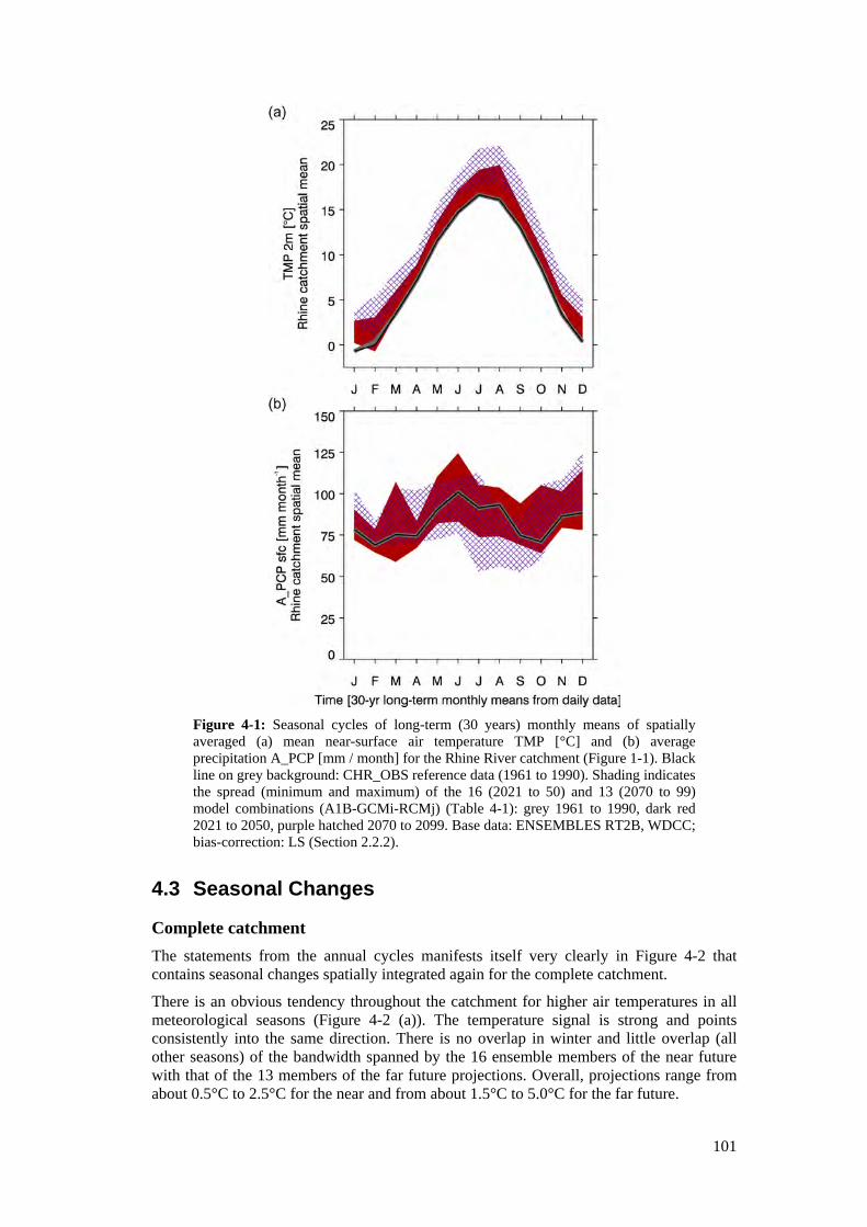
101
Figure 4-1: Seasonal cycles of long-term (30 years) monthly means of spatially averaged (a) mean near-surface air temperature TMP [°C] and (b) average precipitation A_PCP [mm / month] for the Rhine River catchment (Figure 1-1). Black line on grey background: CHR_OBS reference data (1961 to 1990). Shading indicates the spread (minimum and maximum) of the 16 (2021 to 50) and 13 (2070 to 99) model combinations (A1B-GCMi-RCMj) (Table 4-1): grey 1961 to 1990, dark red 2021 to 2050, purple hatched 2070 to 2099. Base data: ENSEMBLES RT2B, WDCC; bias-correction: LS (Section 2.2.2).
4.3 Seasonal Changes
Complete catchment The statements from the annual cycles manifests itself very clearly in Figure 4-2 that contains seasonal changes spatially integrated again for the complete catchment.
There is an obvious tendency throughout the catchment for higher air temperatures in all meteorological seasons (Figure 4-2 (a)). The temperature signal is strong and points consistently into the same direction. There is no overlap in winter and little overlap (all other seasons) of the bandwidth spanned by the 16 ensemble members of the near future with that of the 13 members of the far future projections. Overall, projections range from about 0.5°C to 2.5°C for the near and from about 1.5°C to 5.0°C for the far future.
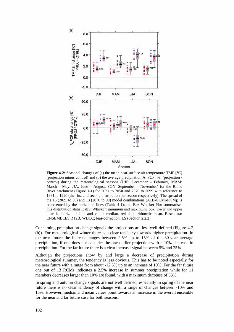
102
Figure 4-2: Seasonal changes of (a) the mean near-surface air temperature TMP [°C] (projection minus control) and (b) the average precipitation A_PCP [%] (projection / control) during the meteorological seasons (DJF: December – February, MAM: March – May, JJA: June – August, SON: September – November) for the Rhine River catchment (Figure 1-1) for 2021 to 2050 and 2070 to 2099 with reference to 1961 to 1990 (the first and second distribution per season respectively). The spread of the 16 (2021 to 50) and 13 (2070 to 99) model combinations (A1B-GCMi-RCMj) is represented by the horizontal lines (Table 4-1); the Box-Whisker-Plot summarises this distribution statistically; Whisker: minimum and maximum, box: lower and upper quartile, horizontal line and value: median, red dot: arithmetic mean. Base data: ENSEMBLES RT2B, WDCC; bias-correction: LS (Section 2.2.2).
Concerning precipitation change signals the projections are less well defined (Figure 4-2 (b)). For meteorological winter there is a clear tendency towards higher precipitation. In the near future the increase ranges between 2.5% up to 15% of the 30-year average precipitation, if one does not consider the one outlier projection with a 10% decrease in precipitation. For the far future there is a clear increase-signal between 5% and 25%.
Although the projections show by and large a decrease of precipitation during meteorological summer, the tendency is less obvious. This has to be noted especially for the near future with a range from about -12.5% up to an increase of 10%. For the far future one out of 13 RCMs indicates a 2.5% increase in summer precipitation while for 11 members decreases larger than 10% are found, with a maximum decrease of 33%.
In spring and autumn change signals are not well defined, especially in spring of the near future there is no clear tendency of change with a range of changes between -10% and 15%. However, median and mean values point towards an increase in the overall ensemble for the near and far future case for both seasons.
103
Figure E-1 in the appendix is similar to Figure 4-2 but it provides a spatially more detailed overview of seasonal air temperature and precipitation changes for the 13 analyses subsets (meteorological regions, Figure 1-1 (b)) within the Rhine River basin. It might be roughly grouped in an Alpine area, subsets along the Rhine River and major tributary areas of the Neckar, Main and Moselle rivers. Within the smaller integration areas the spread within the ensemble becomes particularly obvious for precipitation. Due to the more advective precipitation regimes, which are better captured by the RCMs, the winter season ensemble is hence the least variable. Generally the range and thereby the uncertainty associated with the projections in the far future increases a lot as compared to the near future projections.
Spatial distribution Figure 4-3 and Figure 4-4 show how changes in air temperature and precipitation are spatially distributed throughout the Rhine River basin for the 134 HBV model catchments for the near and far future.
In Figure 4-3 we see for all time-spans and “levels” similar spatial patterns with higher air temperature increases in the South. The magnitude of changes during summer in the near future is about 2°C and about 4°C in the far future. Winter air temperature increases tend to be slightly lower at about 1.5°C and 3°C for the near and far future.
The spatial distribution of precipitation changes in Figure 4-4 is more differentiated. During the near future (Figure 4-4 (a)) most projections point towards an increase during winter up to 10% and during summer towards a decrease of up to -10%. There are projections at the lower end of the ensemble that show a slight decrease during winter, mainly in the South-Western and Alpine parts of the catchment or likewise a stronger decrease west of the Rhine River primarily in the Moselle River catchment in summer.
In the far future the patterns of precipitation change in Figure 4-4 (b) show a by and large uniform pattern with lower change rates in some of the high altitude Alpine catchments (50% level). For the complete catchment and the 10%-level plots there are projections at the lower end of the ensemble that indicate an increase which is lower than 10% (top row, left plot). In contrast, the mid mountain ranges in central Germany (Hunsrück, Taunus and big parts of the Main River catchment) clearly stand out as receiving more precipitation. During summer only a few projections show a decrease of more than 30% (bottom row, left plot), while in most simulations there is a stronger decrease west of the Rhine River of 20% to 30% compared to the 10% to 20% to the east (bottom row, middle plot).
4.4 Robustness of the Precipitation Change Signals
As a change in the precipitation regimes is the most important driver for any change in the hydrological behaviour of rivers, Figure 4-5 shows the number of projections whose precipitation change signal per meteorological season and per calendar year point into the same direction (here: increase) on a per model catchment basis.
In Figure 4-5 (a) for the near future more than half of the ensemble members show an increase in precipitation throughout the catchment when the full calendar year is considered. There is an obvious west-east gradient in the middle and Northern part of the basin and a north-south gradient in the Southern part however, pointing from less to more consistent projections.
Especially for winter there is a rather uniform majority of 17 to 18 RCM projections with a precipitation increase, decreasing towards the Alps.
An increase in precipitation albeit during summer is indicated by just less than half of the 19 RCMs for most of the 134 HBV model catchments; this is again a good indication for the unclear tendencies of precipitation change in the near future.
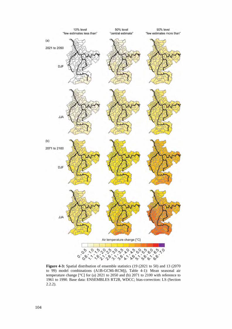
104
Figure 4-3: Spatial distribution of ensemble statistics (19 (2021 to 50) and 13 (2070 to 99) model combinations (A1B-GCMi-RCMj), Table 4-1): Mean seasonal air temperature change [°C] for (a) 2021 to 2050 and (b) 2071 to 2100 with reference to 1961 to 1990. Base data: ENSEMBLES RT2B, WDCC; bias-correction: LS (Section 2.2.2).
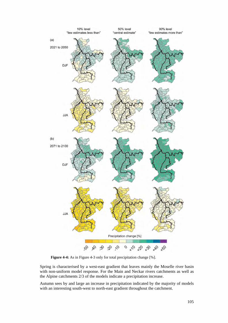
105
Figure 4-4: As in Figure 4-3 only for total precipitation change [%].
Spring is characterised by a west-east gradient that leaves mainly the Moselle river basin with non-uniform model response. For the Main and Neckar rivers catchments as well as the Alpine catchments 2/3 of the models indicate a precipitation increase.
Autumn sees by and large an increase in precipitation indicated by the majority of models with an interesting south-west to north-east gradient throughout the catchment.
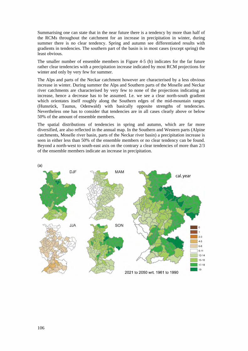
106
Summarising one can state that in the near future there is a tendency by more than half of the RCMs throughout the catchment for an increase in precipitation in winter, during summer there is no clear tendency. Spring and autumn see differentiated results with gradients in tendencies. The southern part of the basin is in most cases (except spring) the least obvious.
The smaller number of ensemble members in Figure 4-5 (b) indicates for the far future rather clear tendencies with a precipitation increase indicated by most RCM projections for winter and only by very few for summer.
The Alps and parts of the Neckar catchment however are characterised by a less obvious increase in winter. During summer the Alps and Southern parts of the Moselle and Neckar river catchments are characterised by very few to none of the projections indicating an increase, hence a decrease has to be assumed. I.e. we see a clear north-south gradient which orientates itself roughly along the Southern edges of the mid-mountain ranges (Hunsrück, Taunus, Odenwald) with basically opposite strengths of tendencies. Nevertheless one has to consider that tendencies are in all cases clearly above or below 50% of the amount of ensemble members.
The spatial distributions of tendencies in spring and autumn, which are far more diversified, are also reflected in the annual map. In the Southern and Western parts (Alpine catchments, Moselle river basin, parts of the Neckar river basin) a precipitation increase is seen in either less than 50% of the ensemble members or no clear tendency can be found. Beyond a north-west to south-east axis on the contrary a clear tendencies of more than 2/3 of the ensemble members indicate an increase in precipitation.
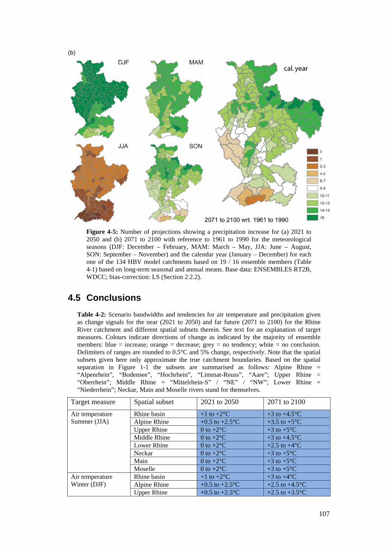
107
Figure 4-5: Number of projections showing a precipitation increase for (a) 2021 to 2050 and (b) 2071 to 2100 with reference to 1961 to 1990 for the meteorological seasons (DJF: December – February, MAM: March – May, JJA: June – August, SON: September – November) and the calendar year (January – December) for each one of the 134 HBV model catchments based on 19 / 16 ensemble members (Table 4-1) based on long-term seasonal and annual means. Base data: ENSEMBLES RT2B, WDCC; bias-correction: LS (Section 2.2.2).
4.5 Conclusions
Table 4-2: Scenario bandwidths and tendencies for air temperature and precipitation given as change signals for the near (2021 to 2050) and far future (2071 to 2100) for the Rhine River catchment and different spatial subsets therein. See text for an explanation of target measures. Colours indicate directions of change as indicated by the majority of ensemble members: blue = increase; orange = decrease; grey = no tendency; white = no conclusion. Delimiters of ranges are rounded to 0.5°C and 5% change, respectively. Note that the spatial subsets given here only approximate the true catchment boundaries. Based on the spatial separation in Figure 1-1 the subsets are summarised as follows: Alpine Rhine = “Alpenrhein”, “Bodensee”, “Hochrhein”, “Limmat-Reuss”, “Aare”; Upper Rhine = “Oberrhein”; Middle Rhine = “Mittelrhein-S” / “NE” / “NW”; Lower Rhine = “Niederrhein”; Neckar, Main and Moselle rivers stand for themselves.
Target measure Spatial subset 2021 to 2050 2071 to 2100
Air temperature Summer (JJA)
Rhine basin +1 to +2°C +3 to +4.5°C Alpine Rhine +0.5 to +2.5°C +3.5 to +5°C Upper Rhine 0 to +2°C +3 to +5°C Middle Rhine 0 to +2°C +3 to +4.5°C Lower Rhine 0 to +2°C +2.5 to +4°C Neckar 0 to +2°C +3 to +5°C Main 0 to +2°C +3 to +5°C Moselle 0 to +2°C +3 to +5°C
Air temperature Winter (DJF)
Rhine basin +1 to +2°C +3 to +4°C Alpine Rhine +0.5 to +2.5°C +2.5 to +4.5°C Upper Rhine +0.5 to +2.5°C +2.5 to +3.5°C
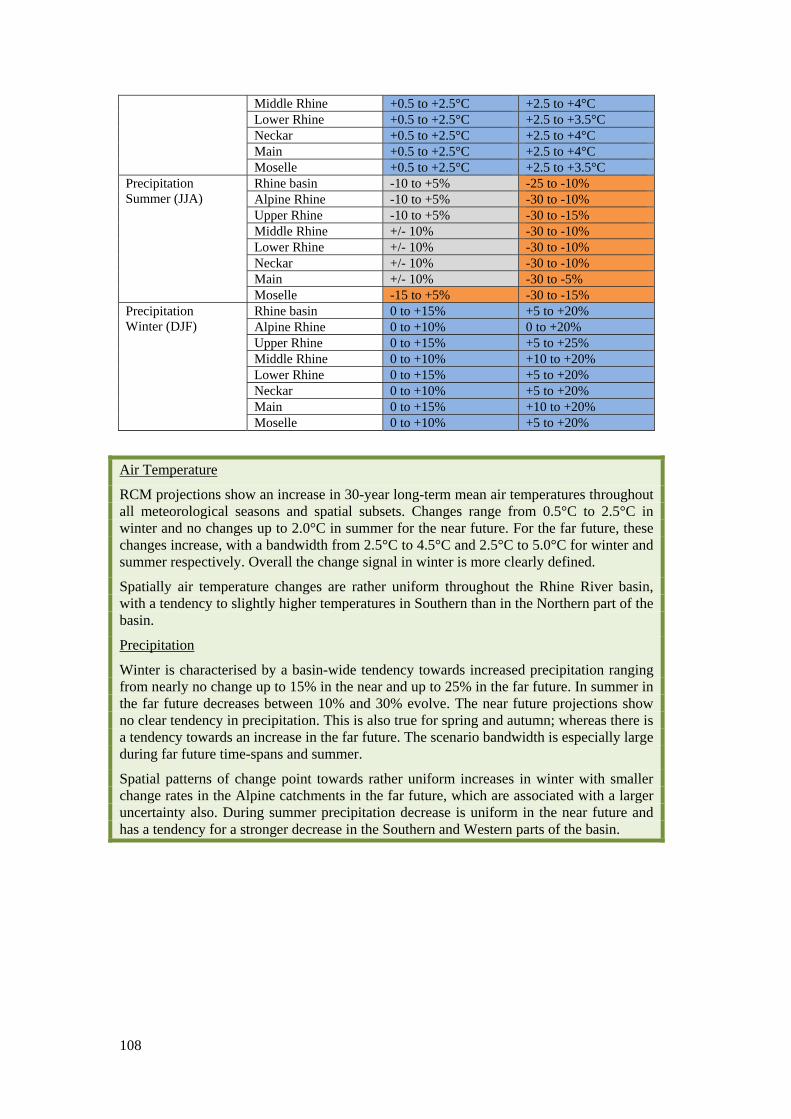
108
Middle Rhine +0.5 to +2.5°C +2.5 to +4°C Lower Rhine +0.5 to +2.5°C +2.5 to +3.5°C Neckar +0.5 to +2.5°C +2.5 to +4°C Main +0.5 to +2.5°C +2.5 to +4°C Moselle +0.5 to +2.5°C +2.5 to +3.5°C
Precipitation Summer (JJA)
Rhine basin -10 to +5% -25 to -10% Alpine Rhine -10 to +5% -30 to -10% Upper Rhine -10 to +5% -30 to -15% Middle Rhine +/- 10% -30 to -10% Lower Rhine +/- 10% -30 to -10% Neckar +/- 10% -30 to -10% Main +/- 10% -30 to -5% Moselle -15 to +5% -30 to -15%
Precipitation Winter (DJF)
Rhine basin 0 to +15% +5 to +20% Alpine Rhine 0 to +10% 0 to +20% Upper Rhine 0 to +15% +5 to +25% Middle Rhine 0 to +10% +10 to +20% Lower Rhine 0 to +15% +5 to +20% Neckar 0 to +10% +5 to +20% Main 0 to +15% +10 to +20% Moselle 0 to +10% +5 to +20%
Air Temperature
RCM projections show an increase in 30-year long-term mean air temperatures throughout all meteorological seasons and spatial subsets. Changes range from 0.5°C to 2.5°C in winter and no changes up to 2.0°C in summer for the near future. For the far future, these changes increase, with a bandwidth from 2.5°C to 4.5°C and 2.5°C to 5.0°C for winter and summer respectively. Overall the change signal in winter is more clearly defined.
Spatially air temperature changes are rather uniform throughout the Rhine River basin, with a tendency to slightly higher temperatures in Southern than in the Northern part of the basin.
Precipitation
Winter is characterised by a basin-wide tendency towards increased precipitation ranging from nearly no change up to 15% in the near and up to 25% in the far future. In summer in the far future decreases between 10% and 30% evolve. The near future projections show no clear tendency in precipitation. This is also true for spring and autumn; whereas there is a tendency towards an increase in the far future. The scenario bandwidth is especially large during far future time-spans and summer.
Spatial patterns of change point towards rather uniform increases in winter with smaller change rates in the Alpine catchments in the far future, which are associated with a larger uncertainty also. During summer precipitation decrease is uniform in the near future and has a tendency for a stronger decrease in the Southern and Western parts of the basin.
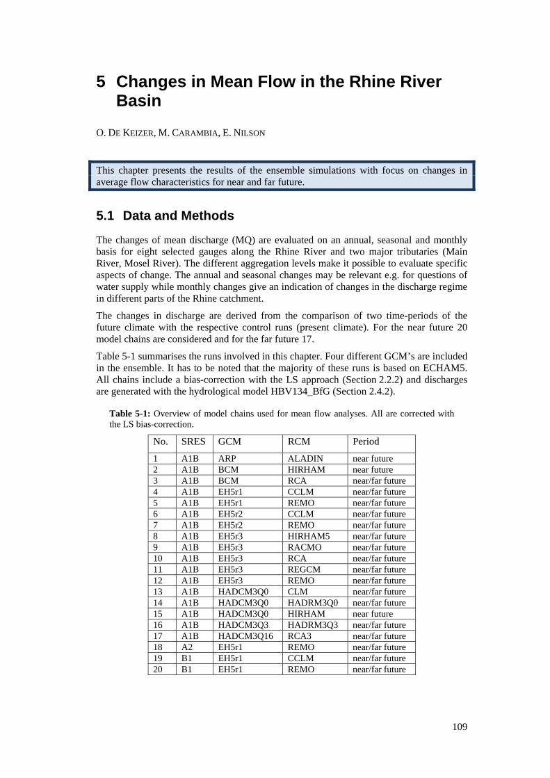
109
5 Changes in Mean Flow in the Rhine River Basin
O. DE KEIZER, M. CARAMBIA, E. NILSON
This chapter presents the results of the ensemble simulations with focus on changes in average flow characteristics for near and far future.
5.1 Data and Methods
The changes of mean discharge (MQ) are evaluated on an annual, seasonal and monthly basis for eight selected gauges along the Rhine River and two major tributaries (Main River, Mosel River). The different aggregation levels make it possible to evaluate specific aspects of change. The annual and seasonal changes may be relevant e.g. for questions of water supply while monthly changes give an indication of changes in the discharge regime in different parts of the Rhine catchment.
The changes in discharge are derived from the comparison of two time-periods of the future climate with the respective control runs (present climate). For the near future 20 model chains are considered and for the far future 17.
Table 5-1 summarises the runs involved in this chapter. Four different GCM’s are included in the ensemble. It has to be noted that the majority of these runs is based on ECHAM5. All chains include a bias-correction with the LS approach (Section 2.2.2) and discharges are generated with the hydrological model HBV134_BfG (Section 2.4.2).
Table 5-1: Overview of model chains used for mean flow analyses. All are corrected with the LS bias-correction.
No. SRES GCM RCM Period
1 A1B ARP ALADIN near future 2 A1B BCM HIRHAM near future 3 A1B BCM RCA near/far future 4 A1B EH5r1 CCLM near/far future 5 A1B EH5r1 REMO near/far future 6 A1B EH5r2 CCLM near/far future 7 A1B EH5r2 REMO near/far future 8 A1B EH5r3 HIRHAM5 near/far future 9 A1B EH5r3 RACMO near/far future 10 A1B EH5r3 RCA near/far future 11 A1B EH5r3 REGCM near/far future 12 A1B EH5r3 REMO near/far future 13 A1B HADCM3Q0 CLM near/far future 14 A1B HADCM3Q0 HADRM3Q0 near/far future 15 A1B HADCM3Q0 HIRHAM near future 16 A1B HADCM3Q3 HADRM3Q3 near/far future 17 A1B HADCM3Q16 RCA3 near/far future 18 A2 EH5r1 REMO near/far future 19 B1 EH5r1 CCLM near/far future 20 B1 EH5r1 REMO near/far future
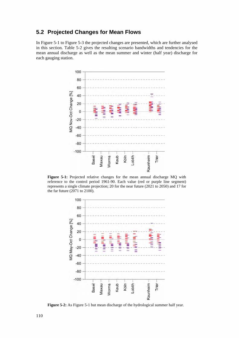
110
5.2 Projected Changes for Mean Flows
In Figure 5-1 to Figure 5-3 the projected changes are presented, which are further analysed in this section. Table 5-2 gives the resulting scenario bandwidths and tendencies for the mean annual discharge as well as the mean summer and winter (half year) discharge for each gauging station.
Figure 5-1: Projected relative changes for the mean annual discharge MQ with reference to the control period 1961-90. Each value (red or purple line segment) represents a single climate projection; 20 for the near future (2021 to 2050) and 17 for the far future (2071 to 2100).
Figure 5-2: As Figure 5-1 but mean discharge of the hydrological summer half year.
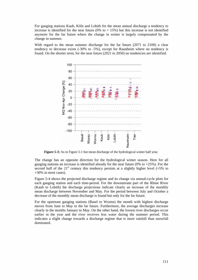
111
For gauging stations Kaub, Köln and Lobith for the mean annual discharge a tendency to increase is identified for the near future (0% to + 15%) but this increase is not identified anymore for the far future where the change in winter is largely compensated by the change in summer.
With regard to the mean summer discharge for the far future (2071 to 2100) a clear tendency to decrease exists (-30% to -5%), except for Raunheim where no tendency is found. On the shorter term, for the near future (2021 to 2050) no tendencies are identified.
Figure 5-3: As in Figure 5-1 but mean discharge of the hydrological winter half year.
The change has an opposite direction for the hydrological winter season. Here for all gauging stations an increase is identified already for the near future (0% to +25%). For the second half of the 21st century this tendency persists at a slightly higher level (+5% to +30% in most cases).
Figure 5-4 shows the projected discharge regime and its change via annual-cycle plots for each gauging station and each time-period. For the downstream part of the Rhine River (Kaub to Lobith) the discharge projections indicate clearly an increase of the monthly mean discharge between November and May. For the period between July and October a decrease of the monthly mean discharge is found but only for the far future.
For the upstream gauging stations (Basel to Worms) the month with highest discharge moves from June to May in the far future. Furthermore, the average discharges increase clearly in the months January to May. On the other hand, the lowest river discharges occur earlier in the year and the river receives less water during the summer period. This indicates a slight change towards a discharge regime that is more rainfall than snowfall dominated.
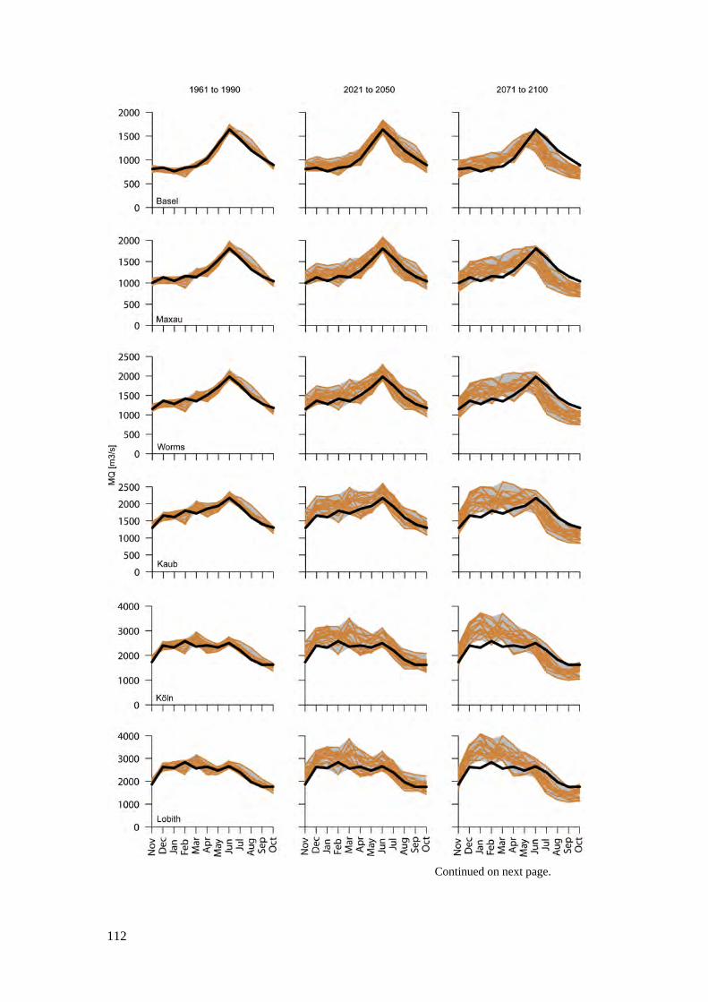
112
Continued on next page.
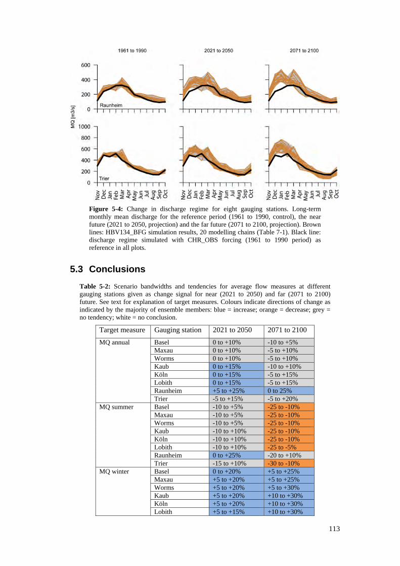
113
Figure 5-4: Change in discharge regime for eight gauging stations. Long-term monthly mean discharge for the reference period (1961 to 1990, control), the near future (2021 to 2050, projection) and the far future (2071 to 2100, projection). Brown lines: HBV134_BFG simulation results, 20 modelling chains (Table 7-1). Black line: discharge regime simulated with CHR_OBS forcing (1961 to 1990 period) as reference in all plots.
5.3 Conclusions
Table 5-2: Scenario bandwidths and tendencies for average flow measures at different gauging stations given as change signal for near (2021 to 2050) and far (2071 to 2100) future. See text for explanation of target measures. Colours indicate directions of change as indicated by the majority of ensemble members: blue = increase; orange = decrease; grey = no tendency; white = no conclusion.
Target measure Gauging station 2021 to 2050 2071 to 2100
MQ annual Basel 0 to +10% -10 to +5% Maxau 0 to +10% -5 to +10% Worms 0 to +10% -5 to +10% Kaub 0 to +15% -10 to +10% Köln 0 to +15% -5 to +15% Lobith 0 to +15% -5 to +15% Raunheim +5 to +25% 0 to 25% Trier -5 to +15% -5 to +20%
MQ summer Basel -10 to +5% -25 to -10% Maxau -10 to +5% -25 to -10% Worms -10 to +5% -25 to -10% Kaub -10 to +10% -25 to -10% Köln -10 to +10% -25 to -10% Lobith -10 to +10% -25 to -5% Raunheim 0 to +25% -20 to +10% Trier -15 to +10% -30 to -10%
MQ winter Basel 0 to +20% +5 to +25% Maxau +5 to +20% +5 to +25% Worms +5 to +20% +5 to +30% Kaub +5 to +20% +10 to +30% Köln +5 to +20% +10 to +30% Lobith +5 to +15% +10 to +30%
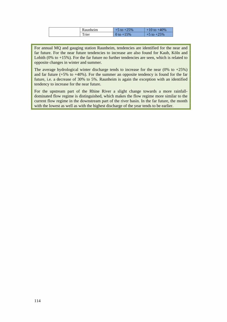
114
Raunheim +5 to +25% +10 to +40% Trier 0 to +15% +5 to +25%
For annual MQ and gauging station Raunheim, tendencies are identified for the near and far future. For the near future tendencies to increase are also found for Kaub, Köln and Lobith (0% to +15%). For the far future no further tendencies are seen, which is related to opposite changes in winter and summer.
The average hydrological winter discharge tends to increase for the near (0% to +25%) and far future (+5% to +40%). For the summer an opposite tendency is found for the far future, i.e. a decrease of 30% to 5%. Raunheim is again the exception with an identified tendency to increase for the near future.
For the upstream part of the Rhine River a slight change towards a more rainfall-dominated flow regime is distinguished, which makes the flow regime more similar to the current flow regime in the downstream part of the river basin. In the far future, the month with the lowest as well as with the highest discharge of the year tends to be earlier.
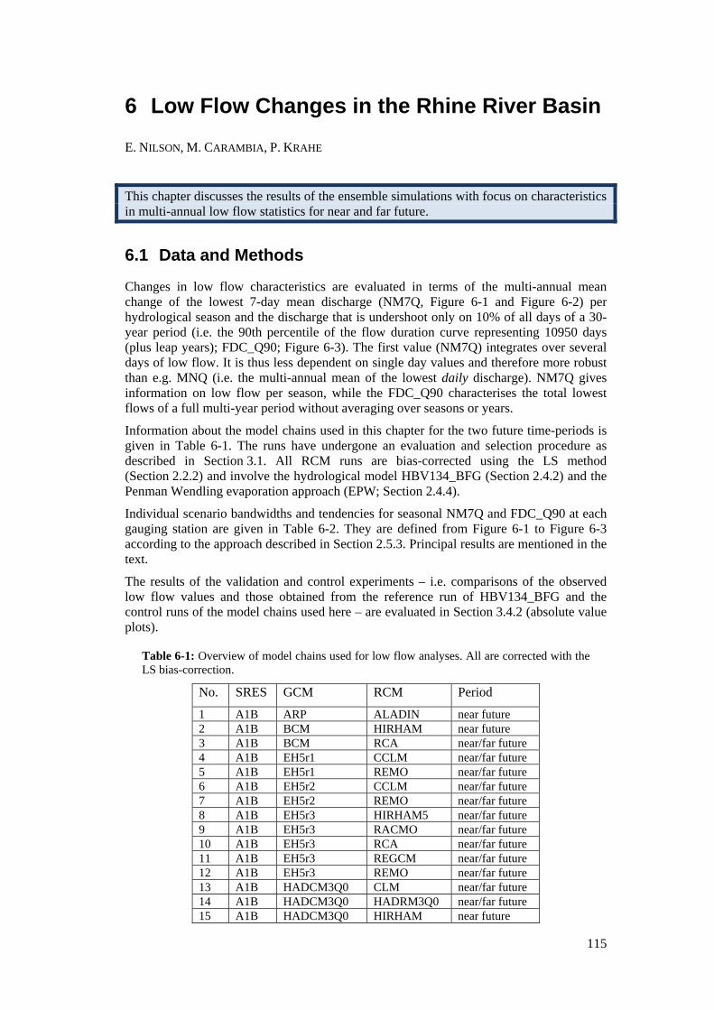
115
6 Low Flow Changes in the Rhine River Basin
E. NILSON, M. CARAMBIA, P. KRAHE
This chapter discusses the results of the ensemble simulations with focus on characteristics in multi-annual low flow statistics for near and far future.
6.1 Data and Methods
Changes in low flow characteristics are evaluated in terms of the multi-annual mean change of the lowest 7-day mean discharge (NM7Q, Figure 6-1 and Figure 6-2) per hydrological season and the discharge that is undershoot only on 10% of all days of a 30-year period (i.e. the 90th percentile of the flow duration curve representing 10950 days (plus leap years); FDC_Q90; Figure 6-3). The first value (NM7Q) integrates over several days of low flow. It is thus less dependent on single day values and therefore more robust than e.g. MNQ (i.e. the multi-annual mean of the lowest daily discharge). NM7Q gives information on low flow per season, while the FDC_Q90 characterises the total lowest flows of a full multi-year period without averaging over seasons or years.
Information about the model chains used in this chapter for the two future time-periods is given in Table 6-1. The runs have undergone an evaluation and selection procedure as described in Section 3.1. All RCM runs are bias-corrected using the LS method (Section 2.2.2) and involve the hydrological model HBV134_BFG (Section 2.4.2) and the Penman Wendling evaporation approach (EPW; Section 2.4.4).
Individual scenario bandwidths and tendencies for seasonal NM7Q and FDC_Q90 at each gauging station are given in Table 6-2. They are defined from Figure 6-1 to Figure 6-3 according to the approach described in Section 2.5.3. Principal results are mentioned in the text.
The results of the validation and control experiments – i.e. comparisons of the observed low flow values and those obtained from the reference run of HBV134_BFG and the control runs of the model chains used here – are evaluated in Section 3.4.2 (absolute value plots).
Table 6-1: Overview of model chains used for low flow analyses. All are corrected with the LS bias-correction.
No. SRES GCM RCM Period
1 A1B ARP ALADIN near future 2 A1B BCM HIRHAM near future 3 A1B BCM RCA near/far future 4 A1B EH5r1 CCLM near/far future 5 A1B EH5r1 REMO near/far future 6 A1B EH5r2 CCLM near/far future 7 A1B EH5r2 REMO near/far future 8 A1B EH5r3 HIRHAM5 near/far future 9 A1B EH5r3 RACMO near/far future 10 A1B EH5r3 RCA near/far future 11 A1B EH5r3 REGCM near/far future 12 A1B EH5r3 REMO near/far future 13 A1B HADCM3Q0 CLM near/far future 14 A1B HADCM3Q0 HADRM3Q0 near/far future 15 A1B HADCM3Q0 HIRHAM near future
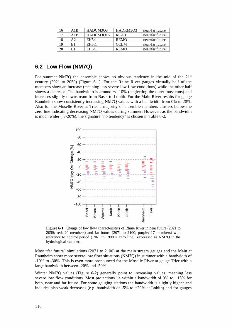
116
16 A1B HADCM3Q3 HADRM3Q3 near/far future 17 A1B HADCM3Q16 RCA3 near/far future 18 A2 EH5r1 REMO near/far future 19 B1 EH5r1 CCLM near/far future 20 B1 EH5r1 REMO near/far future
6.2 Low Flow (NM7Q)
For summer NM7Q the ensemble shows no obvious tendency in the mid of the 21st century (2021 to 2050) (Figure 6-1). For the Rhine River gauges virtually half of the members show an increase (meaning less severe low flow conditions) while the other half shows a decrease. The bandwidth is around +/- 10% (neglecting the outer most runs) and increases slightly downstream from Basel to Lobith. For the Main River results for gauge Raunheim show consistently increasing NM7Q values with a bandwidth from 0% to 20%. Also for the Moselle River at Trier a majority of ensemble members clusters below the zero line indicating decreasing NM7Q values during summer. However, as the bandwidth is much wider (+/-20%), the signature “no tendency” is chosen in Table 6-2.
Figure 6-1: Change of low flow characteristics of Rhine River in near future (2021 to 2050; red; 20 members) and far future (2071 to 2100; purple; 17 members) with reference to control period (1961 to 1990 = zero line); expressed as NM7Q in the hydrological summer.
Most “far future” simulations (2071 to 2100) at the main stream gauges and the Main at Raunheim show more severe low flow situations (NM7Q) in summer with a bandwidth of -10% to -30%. This is even more pronounced for the Moselle River at gauge Trier with a large bandwidth between -20% and -50%.
Winter NM7Q values (Figure 6-2) generally point to increasing values, meaning less severe low flow conditions. Most projections lie within a bandwidth of 0% to +15% for both, near and far future. For some gauging stations the bandwidth is slightly higher and includes also weak decreases (e.g. bandwidth of -5% to +20% at Lobith) and for gauges
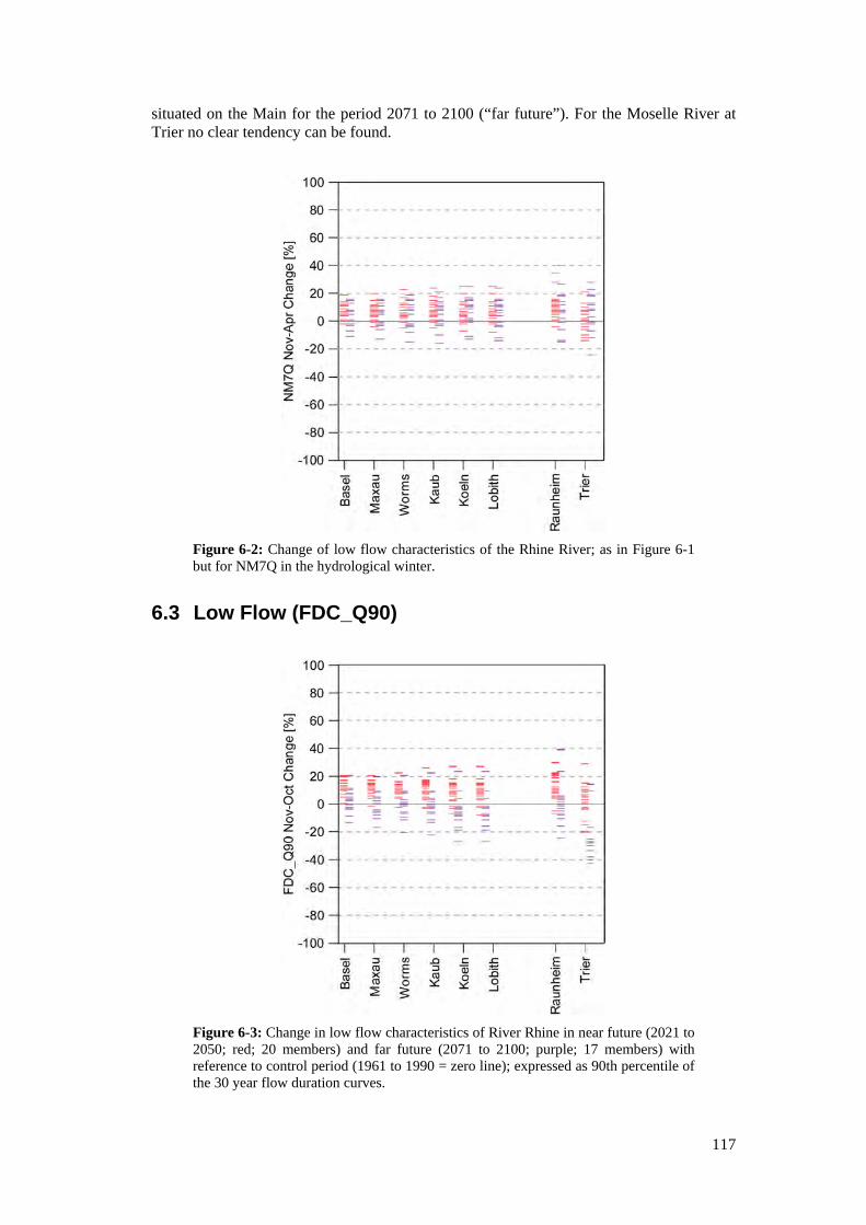
117
situated on the Main for the period 2071 to 2100 (“far future”). For the Moselle River at Trier no clear tendency can be found.
Figure 6-2: Change of low flow characteristics of the Rhine River; as in Figure 6-1 but for NM7Q in the hydrological winter.
6.3 Low Flow (FDC_Q90)
Figure 6-3: Change in low flow characteristics of River Rhine in near future (2021 to 2050; red; 20 members) and far future (2071 to 2100; purple; 17 members) with reference to control period (1961 to 1990 = zero line); expressed as 90th percentile of the 30 year flow duration curves.
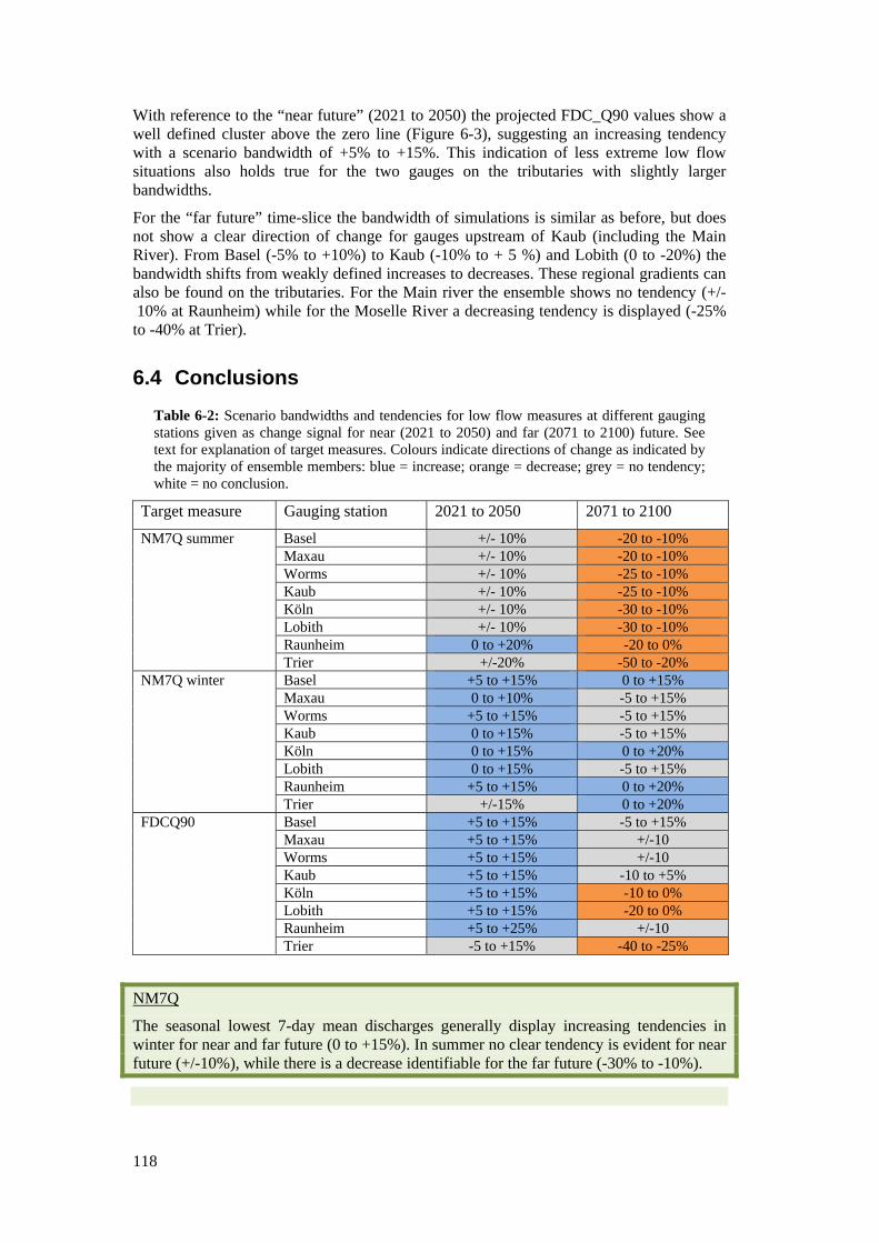
118
With reference to the “near future” (2021 to 2050) the projected FDC_Q90 values show a well defined cluster above the zero line (Figure 6-3), suggesting an increasing tendency with a scenario bandwidth of +5% to +15%. This indication of less extreme low flow situations also holds true for the two gauges on the tributaries with slightly larger bandwidths.
For the “far future” time-slice the bandwidth of simulations is similar as before, but does not show a clear direction of change for gauges upstream of Kaub (including the Main River). From Basel (-5% to +10%) to Kaub (-10% to + 5 %) and Lobith (0 to -20%) the bandwidth shifts from weakly defined increases to decreases. These regional gradients can also be found on the tributaries. For the Main river the ensemble shows no tendency (+/- 10% at Raunheim) while for the Moselle River a decreasing tendency is displayed (-25% to -40% at Trier).
6.4 Conclusions Table 6-2: Scenario bandwidths and tendencies for low flow measures at different gauging stations given as change signal for near (2021 to 2050) and far (2071 to 2100) future. See text for explanation of target measures. Colours indicate directions of change as indicated by the majority of ensemble members: blue = increase; orange = decrease; grey = no tendency; white = no conclusion.
Target measure Gauging station 2021 to 2050 2071 to 2100
NM7Q summer Basel +/- 10% -20 to -10% Maxau +/- 10% -20 to -10% Worms +/- 10% -25 to -10% Kaub +/- 10% -25 to -10% Köln +/- 10% -30 to -10% Lobith +/- 10% -30 to -10% Raunheim 0 to +20% -20 to 0% Trier +/-20% -50 to -20%
NM7Q winter Basel +5 to +15% 0 to +15% Maxau 0 to +10% -5 to +15% Worms +5 to +15% -5 to +15% Kaub 0 to +15% -5 to +15% Köln 0 to +15% 0 to +20% Lobith 0 to +15% -5 to +15% Raunheim +5 to +15% 0 to +20% Trier +/-15% 0 to +20%
FDCQ90 Basel +5 to +15% -5 to +15% Maxau +5 to +15% +/-10 Worms +5 to +15% +/-10 Kaub +5 to +15% -10 to +5% Köln +5 to +15% -10 to 0% Lobith +5 to +15% -20 to 0% Raunheim +5 to +25% +/-10 Trier -5 to +15% -40 to -25%
NM7Q
The seasonal lowest 7-day mean discharges generally display increasing tendencies in winter for near and far future (0 to +15%). In summer no clear tendency is evident for near future (+/-10%), while there is a decrease identifiable for the far future (-30% to -10%).

119
FDC_Q90
The directions of change given by the ensemble for the total flow minima (discharge on the lowest 10% of all days in 30 year periods) at the major gauges along the Rhine point to an increase in near future (+5% to +15% for 2021 to 2050) and show no clear tendency for far future (+/-10% for 2071 to 2010) for the southern gauges from Basel to Kaub. For downstream gauges varying decreases are discernible.

121
7 High Flow Changes in the Rhine River Basin
O. DE KEIZER, J. BEERSMA, R. LAMMERSEN, H. BUITEVELD
This chapter discusses the results of an ensemble of simulations with a focus on changes in high flow characteristics for near and far future.
7.1 Data and Methods
The effect of climate change on extreme high discharges is of particular interest to the countries and the respective water managers of the Rhine River basin, as it is directly related to the safety of its inhabitants and potential economic damage. Hence various norms for the design of the river dikes are established Rhine River basin. For the Rhine River these norms e.g. correspond to a discharge with a return period between 100 in Germany and 1250 years in the Netherlands.
To estimate the effect of climate change on extreme river discharges, often the assumption is made that the relative change in the (monthly) mean is equal to the relative change in the extremes. However, the effect of climate change on peak discharges might be different from the effect on mean discharges.
The changes of high discharge are evaluated here by means of the mean annual maximum discharge (MHQ, the average of all (hydrological) annual maxima in a dataset) and the 10-, 100- and 1000-year return flows (HQ10, HQ100 and HQ1000) for eight selected gauges along the Rhine River and two major tributaries (Main River, Moselle River). The changes are derived from seven model chains by comparison with the respective control runs. All chains include a bias-correction of RCM data following the AS2 approach (Section 2.2.2). Note that this chapter follows a slightly different approach as compared to Chapter 5 and Chapter 6.
In hydrology, the probability that an extreme flow is exceeded is usually expressed as a return period of T-years. This means that the expected number of exceedances in a fixed period of T-years is exactly one. In other words, on average a flood greater than the T-year flood level occurs in a T-year period once [Maidment, 1992]. Assuming that floods are independent from year to year, the probability that the T-year flood level is not exceeded in a T-year period is around 36%. At the same time, the probability that the T-year flood level is exceeded two or more times in a T-year period is 26%.
It is important to mention that extreme flow levels always have wide confidence intervals (Section 3.4). Uncertainties do increase for smaller probabilities; this is also the case for flood analyses based on observed discharge data. Another uncertainty is introduced when the simulated discharge is higher than historical observed maxima because the exact behaviour of the river system outside the range of historically observed discharges is unknown. Mainly for these reasons we will focus here on the projected direction of change rather than the amount of change.
Climate change projections For the high flow analysis seven climate change projections are used, which are shown in Table 7-1. The ensemble includes three different GCMs in various setups and seven different RCMs. Although this selection is just a subset of the full list of available processing chains (Section 2.1.3), it nevertheless represents a large part of the bandwidth contained in the overall RheinBlick2050 ensemble.
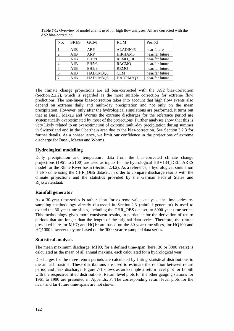
122
Table 7-1: Overview of model chains used for high flow analyses. All are corrected with the AS2 bias-correction.
No. SRES GCM RCM Period
1 A1B ARP ALADIN45 near future 2 A1B ARP HIRHAM5 near/far future 3 A1B EH5r1 REMO_10 near/far future 4 A1B EH5r3 RACMO near/far future 5 A1B EH5r3 REMO near/far future 6 A1B HADCM3Q0 CLM near/far future 7 A1B HADCM3Q3 HADRM3Q3 near/far future
The climate change projections are all bias-corrected with the AS2 bias-correction (Section 2.2.2), which is regarded as the most suitable correction for extreme flow predictions. The non-linear bias-correction takes into account that high flow events also depend on extreme daily and multi-day precipitation and not only on the mean precipitation. However, only after the hydrological simulations are performed, it turns out that at Basel, Maxau and Worms the extreme discharges for the reference period are systematically overestimated by most of the projections. Further analyses show that this is very likely related to an overestimation of extreme multi-day precipitation during summer in Switzerland and in the Oberrhein area due to the bias-correction. See Section 3.2.3 for further details. As a consequence, we limit our confidence in the projections of extreme discharge for Basel, Maxau and Worms.
Hydrological modelling Daily precipitation and temperature data from the bias-corrected climate change projections (1961 to 2100) are used as inputs for the hydrological HBV134_DELTARES model for the Rhine River basin (Section 2.4.2). As a reference, a hydrological simulation is also done using the CHR_OBS dataset, in order to compare discharge results with the climate projections and the statistics provided by the German Federal States and Rijkswaterstaat.
Rainfall generator As a 30-year time-series is rather short for extreme value analysis, the time-series re-sampling methodology already discussed in Section 2.3 (rainfall generator) is used to extend the 30-year time-slices, including the CHR_OBS dataset, to 3000-year time-series. This methodology gives more consistent results, in particular for the derivation of return periods that are longer than the length of the original data series. Therefore, the results presented here for MHQ and HQ10 are based on the 30-year time-slices, for HQ100 and HQ1000 however they are based on the 3000-year re-sampled data series.
Statistical analyses The mean maximum discharge, MHQ, for a defined time-span (here: 30 or 3000 years) is calculated as the mean of all annual maxima, each calculated for a hydrological year.
Discharges for the three return periods are calculated by fitting statistical distributions to the annual maxima. These distributions are used to estimate the relation between return period and peak discharge. Figure 7-1 shows as an example a return level plot for Lobith with the respective fitted distributions. Return level plots for the other gauging stations for 1961 to 1990 are presented in Appendix F. The corresponding return level plots for the near- and far-future time-spans are not shown.
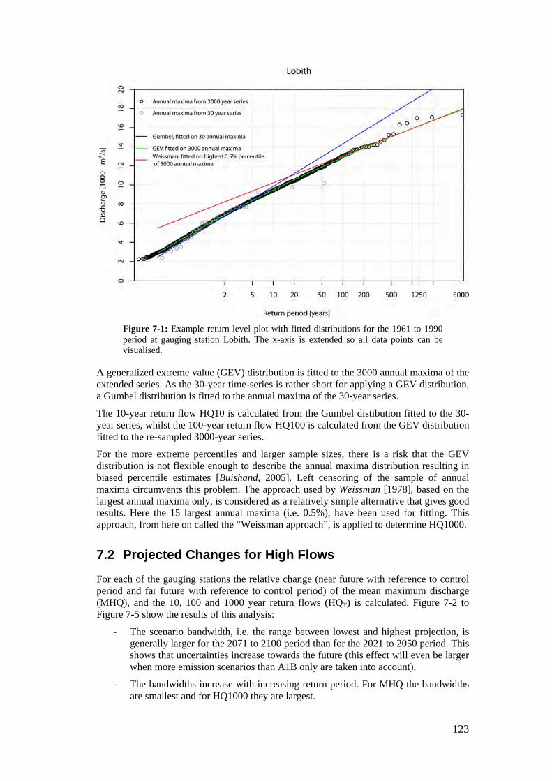
123
Figure 7-1: Example return level plot with fitted distributions for the 1961 to 1990 period at gauging station Lobith. The x-axis is extended so all data points can be visualised.
A generalized extreme value (GEV) distribution is fitted to the 3000 annual maxima of the extended series. As the 30-year time-series is rather short for applying a GEV distribution, a Gumbel distribution is fitted to the annual maxima of the 30-year series.
The 10-year return flow HQ10 is calculated from the Gumbel distibution fitted to the 30-year series, whilst the 100-year return flow HQ100 is calculated from the GEV distribution fitted to the re-sampled 3000-year series.
For the more extreme percentiles and larger sample sizes, there is a risk that the GEV distribution is not flexible enough to describe the annual maxima distribution resulting in biased percentile estimates [Buishand, 2005]. Left censoring of the sample of annual maxima circumvents this problem. The approach used by Weissman [1978], based on the largest annual maxima only, is considered as a relatively simple alternative that gives good results. Here the 15 largest annual maxima (i.e. 0.5%), have been used for fitting. This approach, from here on called the “Weissman approach”, is applied to determine HQ1000.
7.2 Projected Changes for High Flows
For each of the gauging stations the relative change (near future with reference to control period and far future with reference to control period) of the mean maximum discharge (MHQ), and the 10, 100 and 1000 year return flows (HQT) is calculated. Figure 7-2 to Figure 7-5 show the results of this analysis:
- The scenario bandwidth, i.e. the range between lowest and highest projection, is generally larger for the 2071 to 2100 period than for the 2021 to 2050 period. This shows that uncertainties increase towards the future (this effect will even be larger when more emission scenarios than A1B only are taken into account).
- The bandwidths increase with increasing return period. For MHQ the bandwidths are smallest and for HQ1000 they are largest.
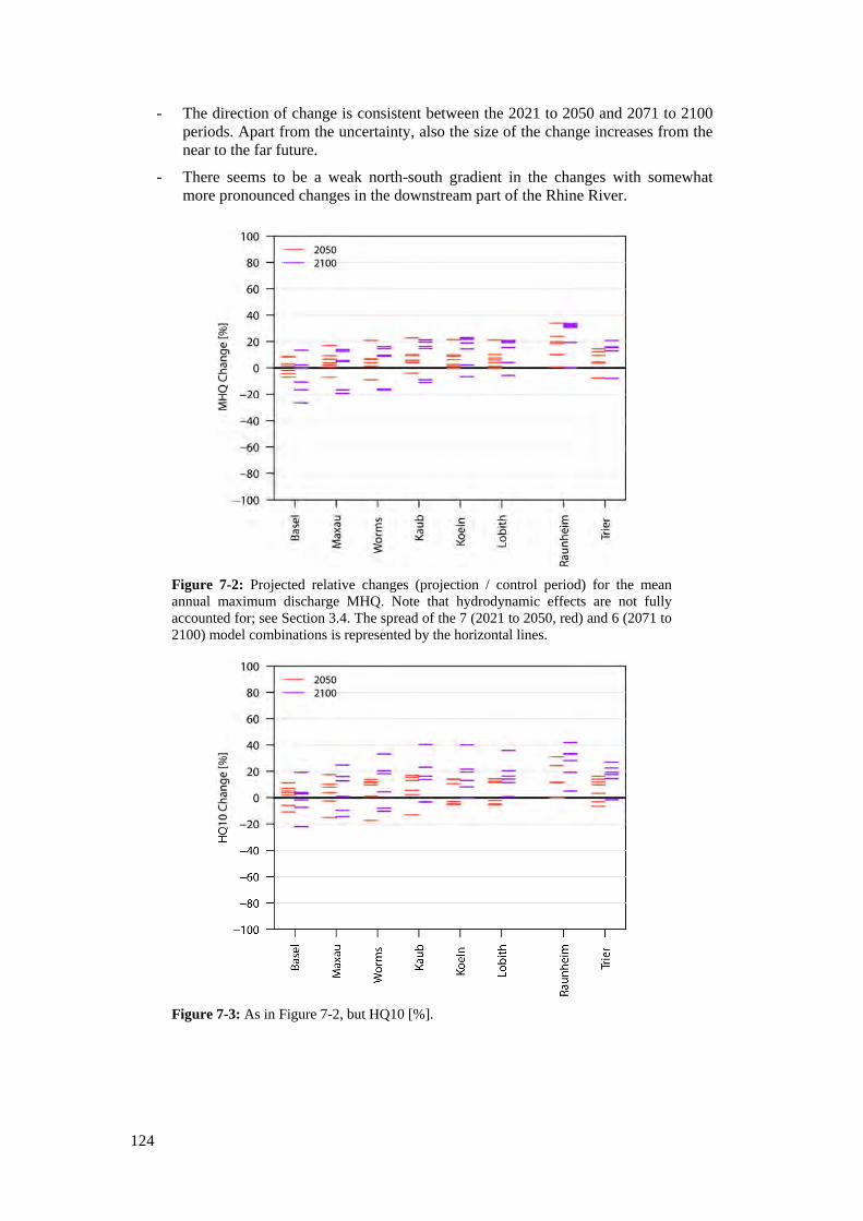
124
- The direction of change is consistent between the 2021 to 2050 and 2071 to 2100 periods. Apart from the uncertainty, also the size of the change increases from the near to the far future.
- There seems to be a weak north-south gradient in the changes with somewhat more pronounced changes in the downstream part of the Rhine River.
Figure 7-2: Projected relative changes (projection / control period) for the mean annual maximum discharge MHQ. Note that hydrodynamic effects are not fully accounted for; see Section 3.4. The spread of the 7 (2021 to 2050, red) and 6 (2071 to 2100) model combinations is represented by the horizontal lines.
Figure 7-3: As in Figure 7-2, but HQ10 [%].
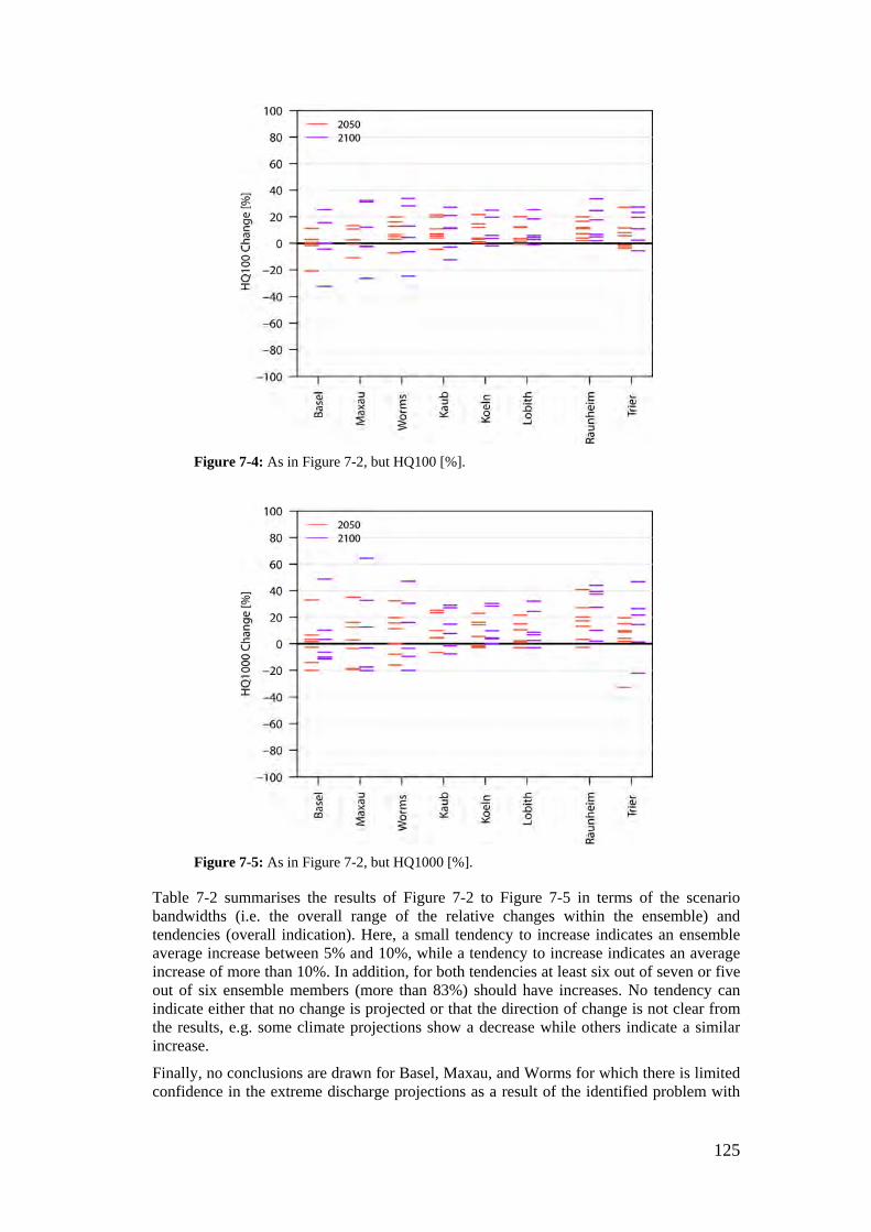
125
Figure 7-4: As in Figure 7-2, but HQ100 [%].
Figure 7-5: As in Figure 7-2, but HQ1000 [%].
Table 7-2 summarises the results of Figure 7-2 to Figure 7-5 in terms of the scenario bandwidths (i.e. the overall range of the relative changes within the ensemble) and tendencies (overall indication). Here, a small tendency to increase indicates an ensemble average increase between 5% and 10%, while a tendency to increase indicates an average increase of more than 10%. In addition, for both tendencies at least six out of seven or five out of six ensemble members (more than 83%) should have increases. No tendency can indicate either that no change is projected or that the direction of change is not clear from the results, e.g. some climate projections show a decrease while others indicate a similar increase.
Finally, no conclusions are drawn for Basel, Maxau, and Worms for which there is limited confidence in the extreme discharge projections as a result of the identified problem with
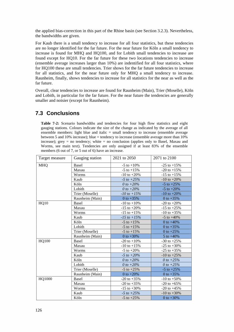
126
the applied bias-correction in this part of the Rhine basin (see Section 3.2.3). Nevertheless, the bandwidths are given.
For Kaub there is a small tendency to increase for all four statistics, but these tendencies are no longer identified for the far future. For the near future for Köln a small tendency to increase is found for MHQ and HQ100, and for Lobith small tendencies to increase are found except for HQ10. For the far future for these two locations tendencies to increase (ensemble average increases larger than 10%) are indentified for all four statistics, where for HQ100 these are small tendencies. Trier shows for the far future tendencies to increase for all statistics, and for the near future only for MHQ a small tendency to increase. Raunheim, finally, shows tendencies to increase for all statistics for the near as well as the far future.
Overall, clear tendencies to increase are found for Raunheim (Main), Trier (Moselle), Köln and Lobith, in particular for the far future. For the near future the tendencies are generally smaller and noisier (except for Raunheim).
7.3 Conclusions
Table 7-2: Scenario bandwidths and tendencies for four high flow statistics and eight gauging stations. Colours indicate the size of the change as indicated by the average of all ensemble members: light blue and italic = small tendency to increase (ensemble average between 5 and 10% increase); blue = tendency to increase (ensemble average more than 10% increase); grey = no tendency; white = no conclusion (applies only to Basel, Maxau and Worms, see main text). Tendencies are only assigned if at least 83% of the ensemble members (6 out of 7, or 5 out of 6) have an increase.
Target measure Gauging station 2021 to 2050 2071 to 2100
MHQ Basel -5 to +10% -25 to +15% Maxau -5 to +15% -20 to +15% Worms -10 to +20% -15 to +15% Kaub -5 to +25% -10 to +20% Köln 0 to +20% -5 to +25% Lobith 0 to +20% -5 to +20% Trier (Moselle) -10 to +15% -10 to +20% Raunheim (Main) 0 to +35% 0 to +35%
HQ10 Basel -10 to +10% -20 to +20% Maxau -15 to +20% -15 to +25% Worms -15 to +15% -10 to +35% Kaub -15 to +15% -5 to +40% Köln -5 to +15% 0 to +40% Lobith -5 to +15% 0 to +35% Trier (Moselle) -5 to +15% 0 to +25% Raunheim (Main) 0 to +30% 5 to +40%
HQ100 Basel -20 to +10% -30 to +25% Maxau -10 to +15% -25 to +30% Worms -5 to +20% -25 to +35% Kaub -5 to +20% -10 to +25% Köln 0 to +20% 0 to +25% Lobith 0 to +20% 0 to +25% Trier (Moselle) -5 to +25% -5 to +25% Raunheim (Main) 0 to +20% 0 to +35%
HQ1000 Basel -20 to +35% -10 to +50% Maxau -20 to +35% -20 to +65% Worms -15 to +30% -20 to +45% Kaub -5 to +25% -10 to +30% Köln -5 to +25% 0 to +30%
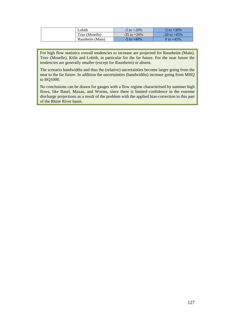
127
Lobith -5 to +20% -5 to +30% Trier (Moselle) -35 to +20% -20 to +45% Raunheim (Main) -5 to +40% 0 to +45%
For high flow statistics overall tendencies to increase are projected for Raunheim (Main), Trier (Moselle), Köln and Lobith, in particular for the far future. For the near future the tendencies are generally smaller (except for Raunheim) or absent.
The scenario bandwidths and thus the (relative) uncertainties become larger going from the near to the far future. In addition the uncertainties (bandwidths) increase going from MHQ to HQ1000.
No conclusions can be drawn for gauges with a flow regime characterised by summer high flows, like Basel, Maxau, and Worms, since there is limited confidence in the extreme discharge projections as a result of the problem with the applied bias-correction in this part of the Rhine River basin.

129
8 Report Summary and Overall Conclusions
This report summary intends to give a wrap-up of the main aspects of the CHR RheinBlick2050 project and summarises the conclusions on the projected changes with respect to meteorological conditions and average, low and high flows.
Research questions and objectives The main research question of the CHR RheinBlick2050 project is: What are the impacts of future climate change on the discharge regimes of the Rhine River and its major tributaries? RheinBlick2050 successfully reaches its core objectives, it:
1. develops a common research framework that is coordinated across countries and institutions in the Rhine River basin;
2. acquires, prepares, generates and evaluates an ensemble of state-of-the-art climate projections for future time-spans and related discharge projections at representative gauges along the Rhine River and major tributaries considering uncertainties;
3. condenses heterogeneous information from various sources into applicable scenario bandwidths and tendencies of possible future changes in meteorological and hydrological key diagnostics.
Research framework, ensemble projections and scenario bandwidths and tendencies Impacts of climate change on the Rhine discharges are assessed using an experiment design with a model chain which starts from GHG emission scenarios, uses global and regional climate models and ends with hydrological modelling. Given the current uncertainties at the individual steps of the model chain, multi-model approaches are regarded as “good practice” [European Commission and Directorate-General for the Environment, 2009]. RheinBlick2050 strictly follows this approach by taking overall initially 37 climate projections (including their respective control runs) from different sources into account. These different realisations of the climate together form a climate ensemble.
These data are subject to an evaluation-selection/correction procedure. During that procedure some model runs turn out to be too biased to be applied in all parts of the study, while the available statistical downscaling projections do not cover the Rhine River basin completely and therefore are discarded.
The regional bias of the different couplings of global and regional climate models that are selected in this study ranges from about 0% to +50% and -2°C to +2°C in monthly mean precipitation and temperature, respectively (25. and 75. quantile of monthly bias values calculated over 134 sub-basins in period 1961 to 1990 excluding outliers). The remaining 20 RCM runs are bias-corrected for 134 individual subcatchments covering the whole Rhine River basin upstream from Lobith. Different bias-correction methods are applied (a) for reasons of comparison but also (b) because different methods are more suitable for different fields of application than others. For example a simple linear scaling approach is sufficient for the evaluation of mean and low flows while non-linear corrections are necessary for high flow simulations and analyses. To assess changes in extreme high flow events, time-series of 3000 years are generated using a resampling-based rainfall generator for a subset of eight (seven up to 2100) bias-corrected climate projections. One of these eight projections is however discarded after all because it contains very unrealistic (extreme) daily precipitation amounts within two of the major Rhine River tributaries (Main and Moselle rivers).
130
A multi-model approach is also applied to the hydrological part. Different hydrological model structures and different model versions of the main model are benchmarked and different parameter sets are compared. The results show, that different model structures lead to a larger spread of results than different parameter sets. However, this spread is still much lower than the spread resulting from the different climate model runs used here.
Out of the comparison of the performance of the hydrological models, only the hydrological model HBV134 is finally selected to generate the ensemble of discharge projections, which means one discharge projection per available RCM control and projection run. The resulting dataset contains between seven (based on non-linear bias-correction and time-series resampling) and 20 ensemble members (based on linear scaling) of daily meteorological and discharge series from 1961 to 2100 (in some cases only until 2050) for eight gauges of the Rhine River and its tributaries. Thirty year time-slices are selected from this discharge series representing the reference period (1961 to 1990), the near future (2021 to 2050) and the far future (2071 to 2100).
Based on the ensemble of discharge projections, the impact of climate change on the Rhine River discharges is expressed in a set of statistical measures which cover a large range of discharges. These diagnostics encompass mean average minimum 7-day flow (NM7Q), the mean discharge (MQ), the monthly mean discharge (MMQ), the mean maximum discharge (MHQ) and the 10, 100 and 1000 year return flows (HQ10, HQ100 and HQ1000). Based on extensive validation experiments, we have the highest confidence in the simulated mean flow statistics (MQ); the simulated low flow statistics values (NM7Q, FDC_Q90) are reasonably reproduced; as expected, extreme discharge statistics show higher uncertainties. Regarding the simulation of high flows the performance of the model chain is considerably better for gauges with winter high flows (Lobith, Köln, Kaub, Raunheim and Trier) than for gauges where high flows occur mostly during summer (Basel, Maxau and Worms). For the latter gauges it is therefore decided not to give interpretations on future high flow projections.
The overall bandwidth of the change signals (i.e. the changes in the respective future projection with reference to its control time-span) within the ensemble is remarkable. For each statistical measure, i.e. diagnostic, the change by the majority of the ensemble members is summarised via scenario bandwidths and tendencies. The latter of which denotes the direction of change: either a tendency to increase or to decrease or no tendency at all. It is important to note that these bandwidths cannot be interpreted in terms of an objective probability of occurrence of specific values. They rather indicate a range that is projected by the selected model couplings as possible.
The following summary is based on the individual conclusions (see analysis tables and green summary boxes) drawn for each analyses chapter in Section 4.5, 5.3, 6.4 and 7.3, respectively.
Meteorology changes Spatially heterogeneous climate change related changes of regional near surface air temperature and precipitation are the key drivers and indicative of any change in the highly interacting terrestrial hydrosphere. This is why we consider meteorological changes as a baseline for further studies on changes in hydrological behaviour of the major rivers in the Rhine River catchment.
RCM projections show an increase in 30-year long-term mean air temperatures throughout all meteorological seasons and spatial subsets. Changes range from 0.5°C to 2.5°C in winter and no changes up to 2.0°C in summer for the near future. For the far future, these changes increase, ranging from 2.5°C to 4.5°C and 2.5°C to 5.0°C for winter and summer respectively. Overall the change signal in winter is more clearly defined.
131
Spatially air temperature changes are rather uniform throughout the Rhine River basin, with a tendency to slightly higher temperatures in Southern than in the Northern part of the basin.
Winter is characterised by a basin-wide tendency towards increased precipitation ranging from nearly no change up to 15% in the near and up to 25% in the far future. In summer in the far future decreases between 10% and 30% evolve. The near future projections show no clear tendency in precipitation. This is also true for spring and autumn; wheras there is a tendency towards an increase in the far future. The scenario bandwidth is especially large during far future time-spans and summer.
Spatial patterns of change point towards rather uniform increases in winter with smaller change rates in the Alpine catchments in the far future, which are associated with a larger uncertainty also. During summer precipitation decrease is uniform in the near future and has a tendency for a stronger decrease in the Southern and Western parts of the basin.
Average discharge changes The annual and seasonal mean discharge may be relevant e.g. for questions of water supply while monthly changes give an indication of changes in the discharge regime in different parts of the Rhine catchment.
The average discharge (MQ) indicates general trends in the future discharge regime, in particular the average winter and summer discharges change.
For the average annual discharge and gauging station Raunheim, tendencies are identified for the near and far future. For the near future tendencies to increase are also found for Kaub, Köln and Lobith (0% to +15%). For the far future no further tendencies are seen, which is related to opposite changes in winter and summer.
The average hydrological winter discharge tends to increase for the near (0% to +25%) and far future (+5% to +40%). For the summer an opposite tendency is found but only for the far future, i.e. a decrease of 30% to 5%; Raunheim is again the exception with an identified tendency to increase albeit for the near future (no tendency in the far future).
For the upstream part of the Rhine River a slight change towards a more rainfall-dominated flow regime is distinguished, which makes the flow regime more similar to the current flow regime in the downstream part of the river basin. In the far future, the month with the lowest as well as with the highest discharge of the year tends to be earlier.
Low flow changes Low flow is of high relevance for various functions of the Rhine River. Most of all, ecosystems and economical functions are sensitive to limited water availability. Two low flow measures are selected to evaluate the change in near (2021 to 2050) and far future (2071 to 2100) with respect to the control period from 1961 to 1990: NM7Q displays the lowest 7-day mean flows (averaged over 30 years), FDC_Q90 reflects the 10% total lowest flows over all days of a 30-year period.
For the near future the scenario bandwidths and tendencies identified for the two low flow measures show either no clear tendencies as for NM7Q in summer with +/-10% or less severe low flow conditions as is shown in a bandwidth and direction of change of 0% to +15% for NM7Q during winter and FDC_Q90. For the far future a decrease of low flows is obvious in summer with -25% to 0% for summer for NM7Q, while for winter no clear NM7Q change signal can be captured. With respect to FDC_Q90 there is no clear signal for the far future. Some gauges show decreases, others show no clear tendency of change.
The two gauges on the tributaries Main and Moselle deviate from the above picture. The bandwidths are generally higher than for the gauges along the Rhine River.
132
High flow changes The effect of climate change on floods is of special interest to the riparian countries of the Rhine River, as it is directly related to the safety of its inhabitants and potential economic damage.
For high flow statistics overall tendencies to increase are projected for Raunheim (Main), Trier (Moselle), Köln and Lobith, in particular for the far future. For the near future the tendencies are generally smaller (except for Raunheim) or absent.
The scenario bandwidths and thus the (relative) uncertainties become larger going from the near to the far future. In addition the uncertainties (bandwidths) increase going from MHQ to HQ1000.
No conclusions can be drawn for gauges with a flow regime characterised by summer high flows, like Basel, Maxau, and Worms, since there is limited confidence in the extreme discharge projections as a result of the problem with the applied bias-correction in this part of the Rhine River basin.
Synopsis Based on a consistent experiment design a joint, concerted, international view of climate change impacts on the discharge regime of the Rhine River is derived. There are different magnitudes of uncertainties and reliabilities assigned to the individual results for average, low and high flow. The hydrological projections presented here are based on the current understanding of the climate system and the hydrology of the Rhine River basin. Besides uncertainties there are limitations and there may be scientific unknowns that could affect the changes presented. These projections should be seen as possible projections rather than absolute predictions or forecasts of the hydrology of the Rhine River for the future climate. Further, these projections are based on state-of-the-art knowledge and methodologies at the summer of 2010, but since this area of science is developing fast the “best before date” is limited. The discharge analyses are intended to foster the ongoing discussion on the dimension of vulnerability and the necessity for adaptation of ecological and economical systems dependent on the Rhine River. However, these projections clearly are not the one and only solution to the “climate problem”, if there is one.
9 Outlook
In this chapter we identify issues that pose needs for future research and developments. The limitations mentioned in the preceding chapters clearly indicate, that the RheinBlick2050 framework has to be subject to further critical discussion. Part of this discussion has already begun. How much bias-correction is allowed? What is the best modelling approach to assess changes of extreme discharges? Will there be an “ideal” model chain in the near future?
The climate impact community expects further improvements from the new model runs for the upcoming 5th IPCC assessment report (scheduled for 2013), which are currently underway e.g. with new global models and new greenhouse gas emission scenarios in CMIP5 [Meehl, et al., 2007] and regional models within CORDEX [Giorgi, et al., 2009]. That is, models are increasingly able to reproduce the complex dynamics and interactions of the various subsystems of the natural and human environment.
The next generation of global “earth system models” will include advanced carbon cycle and atmospheric chemistry modules. This means, that those model systems are more realistic and better capture bio-geo-chemical cycles, which means also higher degrees of freedom. However this might result in an increase in bandwidth, but it makes us more confident, that the “real” (unknown) future evolution of the atmosphere is within the models’ bandwidths.
Increasing computational resources allow not only for a more comprehensive representation of real-world processes but also for an increase in the spatial resolution of global and regional climate models alike. This results in a better representation of surface heterogeneities (e.g. land-use or orography) and physical processes (e.g. convection, cloud formation, precipitation, dynamics in complex topography). This may lead to improved model results that help to better capture extreme events and also limit the need for and the amount of bias-corrections.
However, as the current state of the art in climate modelling is far from producing unbiased climate projections, a clear need exists for further development of bias-correction methods. Also research is needed on objective criteria to evaluate climate projections from a hydrological point of view. In order to address hydrological extremes the development of stochastical wheather generators seems required.
Also the “real world” monitoring data products need to be improved. Different meteorological observation products clearly deviate from each other due to different station densities and processing procedures (e.g. error detection, error correction, systematic instrument errors, interpolation). Meteorological and hydrological observations act as the reference for any change analysis and are an essential prerequisite for model development. Statistical downscaling approaches as well as advanced bias-correction methods are largely dependent on valid observation products.
In analogue to the RCM ensemble studies, hydrological model intercomparisons have to become routine in quantifying and evaluating model uncertainties in the framework of climate impact analyses. RheinBlick2050 has given a start here. Anyway, the validity of the hydrological models under unprecedented circumstances as a result of the changing climate (e.g. evaporation) has to be analysed in more detail.
Still some shortcomings exist with regard to the hydrological model of the Rhine River basin HBV134 used in this study which have to be further investigated. Furthermore from an adaptation perspective, water resource management systems as well as sophisticated hydrodynamic modelling to consider flood routing processes together with flood retention measures have to be used. The latter is of special importance if an assessment of extreme discharge is of interest.
134
As uncertainties in the future behaviour of a water system under climate change are inherent, besides an effort to reduce this uncertainty it is also imperative to strengthen the scientific basis for dealing with uncertainties in climate change from an adaptation perspective. The definition and use of critical thresholds for decision making processes is an example to be mentioned here.
As a consequence, we are aware, that studies like RheinBlick2050 do not give final answers. Nevertheless, RheinBlick2050 is a step forward since it provides stakeholders and impact scenario users with ensemble projections, resulting scenario bandwidths and tendencies rather than single “solutions”. These results can be used to back-up relevant (policy) options that are considered now and in the near future. The international cooperation within the RheinBlick2050 project assures that this backup has a common basis at the river basin level. The framework of RheinBlick2050 is solid and future studies will build on this framework, mainly by using improved (model) components.
135
References
AdaptAlp (2010), Project Homepage, http://www.adaptalp.org, 2010-09-14.
Andréassian, V., Oddos, A., Michel, C., Anctil, F., Perrin, C., and Loumagne, C. (2004), Impact of spatial aggregation of inputs and parameters on the efficiency of rainfall-runoff models: A theoretical study using chimera watersheds, Water Resources Research, 40, W05209, doi:05210.01029/02003WR002854.
Andréassian, V., Perrin, C., Berthet, L., Le Moine, N., Lerat, J., Loumagne, C., Oudin, L., Mathevet, T., Ramos, M. H., and Valéry, A. (2009), Crash tests for a standardized evaluation of hydrological models, Hydrol. Earth. Syst. Sci., 13, 1757-1764.
Arnold, J., Pall, P., Bosshard, T., Kotlarski, S., and Schär, C. (2009), Detailed study of heavy precipitation events in the Alpine region using ERA40 driven RCMs, ENSEMBLES Deliverable, D5.32, 49 pp, ETH Zurich.
ATV-DVWK (2002), Verdunstung in Bezug zu Landnutzung, Bewuchs und Boden, Merkblatt ATV-DVWK, M504, Hennef.
Bates, B. C., Kundzewicz, Z. W., Wu, S., and Palutikof, J. P. (2008), Climate Change and Water, Technical Paper of the Intergovernmental Panel on Climate Change, 210 pp, Geneva.
Beersma, J. J. (2002), Rainfall generator for the Rhine Basin; Description of 1000-year simulations, KNMI publication, PUBL-186-V.
Beersma, J. J., and Buishand, T. A. (2003), Multi-site simulation of daily precipitation and temperature conditional on the atmospheric circulation, Climate Research, 25, 121-133.
Belz, J. U., Brahmer, G., Buiteveld, H., Engel, H., Grabher, R., Hodel, H., Krahe, P., Lammersen, R., Larina, M., Mendel, H.-G., Meuser, A., Müller, G., Plonka, B., Pfister, L., and van Vuuren, W. (2007), Das Abflussregime des Rheins und seiner Nebenflüsse im 20. Jahrhundert. Analyse, Veränderungen und Trends, CHR report series, I-22, 395 pp, International Commission for the Hydrology of the Rhine Basin, Lelystad.
Bergström, S. (1976), Development and application of a conceptual runoff model for Scandinavian catchments, SMHI Reports RHO, 7, Norrköping.
Bergström, S. (1995), The HBV model, in Computer Models of Watershed Hydrology, Chapter 13, edited by Singh, V. P., pp. 443-476, Water Resources Publications.
Bergström, S., and Forsman, A. (1973), Development of a conceptual deterministic rainfall-runoff model, Nordic Hydrology, 4, 147-170.
Beven, K. J., and Kirkby, M. J. (1979), A physically based, variable contributing area model of basin hydrology, Hydrological Sciences Bulletin, 24, 43-69.
Brahmer, G. (2007), Klimawandel und seine Konsequenzen für die Wasserwirtschaft in Hessen, paper presented at 3. KLIWA Symposium am 25. und 26.10.2006 in Stuttgart – Klimaveränderung und Konsequenzen für die Wasserwirtschaft, Arbeitskreis KLIWA, Stuttgart.
Bronstert, A., Kolokotronis, V., Schwandt, D., and Straub, H. (2007), Comparison and evaluation of regional climate scenarios for hydrological impact analysis: General scheme and application example, International Journal of Climatology, 27, 1579-1594.
Buishand, T. A. (2005), Estimation of Large Percentiles from Censored Data, KNMI.
136
Buishand, T. A., and Brandsma, T. (2001), Multi-site simulation of daily precipitation and temperature in the Rhine basin by nearest-neighbor resampling, Water Resources Research, 37, 2761-2776.
Buishand, T. A., and Lenderink, G. (2004), Estimation of future discharges of the river Rhine in the SWURVE project, TR -273, 43 pp.
Bülow, K., Jacob, D., and Tomassini, L. (2009), Vergleichende Analysen regionaler Klimamodelle für das heutige und zukünftige Klima, paper presented at KLIWAS - Auswirkungen des Klimawandels auf Wasserstraßen und Schifffahrt in Deutschland, BMVBS, Bonn.
Caesar, J., Alexander, L., and Vose, R. (2006), Large-scale changes in observed daily maximum and minimum temperatures: Creation and analysis of a new gridded data set, Journal of Geophysical Research, 111, D05101.
Castellari, S. (2008), ClimChAlp – Climate Change Assessment Report, 179 pp.
Christensen, J., Carter, T., Rummukainen, M., and Amanatidis, G. (2007), Evaluating the performance and utility of regional climate models: the PRUDENCE project, Climatic Change, 81, 1-6.
Conference of Rhine Ministers (2007), Living and linking Rhine – common challenge of a watershed, in Communiqué of the 14th conference of Rhine ministers, edited, p. 9, International Commission for the Protection of the Rhine, Bonn.
Dällenbach, F. (2000), Gebietsniederschlag Schweiz - Interpolation und Berechnung der Niederschlagsdaten, in Expert's report by METEOTEST for the Landeshydrologie und -geologie (LHG), edited, Bern.
Deutscher Bundestag (2008), Deutsche Anpassungsstrategie an den Klimawandel, Drucksache 16/11595, p. 52, www.bmu.de/klimaschutz/downloads/doc/42783.php.
Diermanse, F. L. M. (2004), HR2006 - herberekening werklijn Rijn, WL, Delft.
Donnelly-Makowecki, L. M., and Moore, R. D. (1999), Hierarchical testing of three rainfall-runoff models in small forested catchments, Journal of Hydrology, 219, 136-152.
Eberle, M., Buitefeld, H., Wilke, K., and Krahe, P. (2005), Hydrological Modelling in the River Rhine Basin, Part III-Daily HBV Model for the Rhine Basin, BfG-Berichte, BfG-1451, Federal Institute of Hydrology, Koblenz.
Edijatno, Nascimento, N. O., Yang, X., Makhlouf, Z., and Michel, C. (1999), GR3J: a daily watershed model with three free parameters, Hydrological Sciences Journal, 44, 263-277.
Ekström, M., Hingray, B., Mezghani, A., and Jones, P. D. (2007), Regional climate model data used within the SWURVE project - 2: addressing uncertainty in regional climate model data for five European case study areas, Hydrol. Earth Syst. Sci., 11, 1085-1096.
European Commission, and Directorate-General for the Environment (2009), Common Implementation Strategy for the Water Framework Directive (2000/60/EC) – River basin management in a changing climate (Guidance Document No. 24), Technical Report - 2009 - 040, 24, 131 pp.
FLOW-MS (2010), Project Homepage, http://www.flow-ms.eu, 2010-09-14.
Fortin, V., and Turcotte, R. (2007), Le modèle hydrologique MOHYSE, Note de cours pour SCA7420, Université du Québec à Montréal : Département des sciences de la terre et de l'atmosphère.
Fowler, H. J., Blenkinsop, S., and Tebaldi, C. (2007), Linking climate change modelling to impacts studies: recent advances in downscaling techniques for hydrological modelling, International Journal of Climatology, 27, 1547-1578.
137
Frei, C., and Schär, C. (1998), A precipitation climatology of the Alps from high-resolution rain-gauge observations, International Journal of Climatology, 18, 873-900.
Garçon, R. (1996), Prévision opérationnelle des apports de la Durance à Serre-Ponçon à l'aide du modèle MORDOR, La Houille Blanche, 5, 71-76.
Giorgi, F., Jones, C., and Asrar, G. R. (2009), Addressing climate information needs at the regional level: the CORDEX framework, WMO Bulletin, 58, 175-183.
Goodess, C. M., Jacob, D., Déqué, M., Guttiérrez, J. M., Huth, R., Kendon, E., Leckebusch, G. C., Lorenz, P., and Pavan, V. (2009), Downscaling methods, data and tools for input to impacts assessments, in ENSEMBLES: Climate Change and its Impacts: Summary of research and results from the ENSEMBLES project, edited by van der Linden, P. and Mitchell, J. F. B., pp. 59-78, Exeter EX1 3PB, UK.
Grabs, W., Daamen, K., Gellens, D., Kwadijk, J. C. J., Lang, H., Middelkoop, H., Parmet, B. W. A. H., Schädler, B., Schulla, J., and Wilke, K. (1997), Impact of Climate Change on Hydrological Regimes and Water Resources Management in the Rhine Basin, CHR reports series, I-16, Lelystad.
Graham, L. P., S., H., Jaun, S., and Beniston, M. (2007), On interpreting hydrological change from regional climate models, Climatic Change, 81, 97-122.
Hagemann, S., Machenhauer, B., Jones, R., Christensen, O. B., Déqué, M., Jacob, D., and Vidale, P. L. (2004), Evaluation of water and energy budgets in regional climate models applied over Europe, Climate Dynamics, 23, 547-567.
Haylock, M. R., Hofstra, N., Klein Tank, A. M. G., Klok, E. J., Jones, P. D., and New, M. (2008), A European daily high-resolution gridded data set of surface temperature and precipitation for 1950–2006, Journal of Geophysical Research, 113, D20119.
Helbig, A. (2004), Analyse der raum-zeitlichen Struktur täglicher Niederschlagssummen in ausgewählten Teileinzugsgebieten des Rheins unter besonderer Berücksichtigung der Hochwasserereignisse im Zeitraum 1961-1998 CHR-Report, I-21, Lelystad.
Hurkmans, R., Terink, W., Uijlenhoet, R., Torfs, P., Jacob, D., and Troch, P. A. (2010), Changes in Streamflow Dynamics in the Rhine Basin under Three High-Resolution Regional Climate Scenarios, Journal of Climate, 23, 679-699.
IKSR (2009), Analyse des Kenntnisstands zu den bisherigen Veränderungen des Klimas und zu den Auswirkungen der Klimaänderung auf den Wasserhaushalt im Rhein-Einzugsgebiet - Literaturauswertung Stand Anfang 2009, IKSR Bericht 174, IKSR Bericht, 174, 67 pp, Koblenz.
IPCC (2007a), Climate Change 2007: Synthesis Report, Fourth Assessment – Climate Change 2007, 52 pp.
IPCC (2007b), Climate Change 2007: The Physical Science Basis. Contribution of Working Group I of the Fourth Assessment Report (AR4) of the Intergovernmental Panel on Climate Change, 996 pp., Cambridge University Press, Cambridge, United Kingdom, New York, NY, USA.
IPCC (2007c), Summary for Policymakers, in Climate Change 2007: The Physical Science Basis. Contribution of Working Group I to the Fourth Assessment Report of the Intergovernmental Panel on Climate Change, edited by Solomon, S., Qin, D., Manning, M., Chen, Z., Marquis, M., Averyt, K. B., Tignor, M. and Miller, H. L., Cambridge University Press, Cambridge, UK, New York, NY, USA.
Jacob, D., Bärring, L., Christensen, O. B., Christensen, J. H., de Castro, M., Déqué, M., Giorgi, F., Hagemann, S., Hirschi, M., Jones, R., Kjellström, E., Lenderink, G., Rockel, B., Sánchez, E., Schär, C., Seneviratne, S. I., Somot, S., van Ulden, A., and van den Hurk,
138
B. (2007), An inter-comparison of regional climatemodels for Europe: model performance in present-day climate, Climatic Change, 81, 31-52.
Jacob, D., Göttel, H., Kotlarski, S., Lorenz, P., and Sieck, K. (2008), Klimaauswirkungen und Anpassung in Deutschland – Phase 1: Erstellung regionaler Klimaszenarien für Deutschland, Forschungsbericht 204 41 138 UBA-FB 000969, 159 pp, Umweltbundesamt.
Jakeman, A. J., Littlewood, I. G., and Whitehead, P. G. (1990), Computation of the instantaneous unit hydrograph and identifiable component flows with application to two small upland catchments, Journal of Hydrology, 117, 275-300.
Jiang, T., Chen, Y. Q. D., Xu, C. Y. Y., Chen, X. H., Chen, X., and Singh, V. P. (2007), Comparison of hydrological impacts of climate change simulated by six hydrological models in the Dongjiang Basin, South China, Journal of Hydrology, 336, 316-333.
JRC/MARS Interpolated meteorological data, edited, JRC/MARS - Meteorological Data Base - EC - JRC.
Kay, A. L., and Davies, H. N. (2008), Calculating potential evaporation from climate model data: A source of uncertainty for hydrological climate change impacts, Journal of Hydrology, 358, 221-239.
Kilsby, C. G. (2007), HESS Special Issue: Sustainable Water: Uncertainty, Risk and Vulnerability in Europe – Context and Aims, Hydrology and Earth System Sciences, Special Issue, 11, 1065-1068.
Kleinn, J., Frei, C., Gurtz, J., Lüthi, D., Vidale, P. L., and Schär, C. (2005), Hydrologic simulations in the Rhine basin driven by a regional climate model, Journal of Geophysical Research, 110, D04102.
Klemeš, V. (1986), Operational testing of hydrological simulation models, Hydrological Sciences Journal, 31, 13-24.
KlimaLandRP (2010), Project Homepage, http://www.klimlandrp.de/, 2010-09-14.
KLIWA (2010), 4. KLIWA Symposium am 3. und 4. Dezember 2009 in Mainz – Klimaveränderung und Konsequenzen für die Wasserwirtschaft, KLIWA Berichte, 313 pp.
Koutsoyiannis, D. (2006), Nonstationarity versus scaling in hydrology, Journal of Hydrology, 324, 239-254.
Krahe, P., Eberle, M., Carambia, M., Buitefeld, H., and Wilke, K. (unpublished), A hydrometeorological reference data set for the river Rhine ("CHR_OBS"), BfG-Berichte, Federal Institute of Hydrology, Koblenz.
Krahe, P., Nilson, E., Carambia, M., Maurer, T., Tomassini, L., Bülow, K., Jacob, D., and Moser, H. (2009), Wirkungsabschätzung von Unsicherheiten der Klimamodellierung in Abflussprojektionen - Auswertung eines Multimodell-Ensembles im Rheingebiet, Hydrologie und Wasserbewirtschaftung, 316-331.
Krahe, P., Rachimow, C., Richter, K., and Schwarze, R. (2006), Abflussganglinienanalyse im Rheingebiet zur prozessorientierten Parameterbestimmung für ein makroskaliges semi-distributives N-A-Modell, Dresdner Schriften zur Hydrologie, 5, 233-241 pp, Dresden.
Kundzewicz, Z. W., Mata, L. J., Arnell, N. W., Döll, P., Kabat, P., Jiménez, B., Miller, K. A., Oki, T., Sen, Z., and Shiklomanov, I. A. (2007), Freshwater resources and their management, in Climate Change 2007: Impacts, Adaptation and Vulnerability. Contribution of Working Group II to the Fourth Assessment Report of the Intergovernmental Panel on Climate Change, edited by Parry, M. L., Canziani, O. F., Palutikof, J. P., van der Linden, P. J. and Hanson, C. E., pp. 173-210, Cambridge University Press,, Cambridge, UK.
139
Kwadijk, J., and Rotmans, J. (1995), The impact of climate change on the river Rhine: a scenario study, Climatic Change, 30, 397-426.
Lall, U., and Sharma, A. (1996), A nearest neighbor bootstrap for resampling hydrologic time series, Water Resources Research, 32, 679-693.
Landesanstalt für Umwelt, M. u. N. B.-W. (2005), Deutsches Gewässerkundliches Jahrbuch: Rheingebiet, Teil I: Hoch - und Oberrhein, Deutsches Gewässerkundliches Jahrbuch, Karlsruhe.
Landesumweltamt Nordrhein-Westfalen (2005), Deutsches Gewässerkundliches Jahrbuch: Rheingebiet, Teil III: Mittel- und Niederrhein mit deutschem Issel- und Maasgebiet, Deutsches Gewässerkundliches Jahrbuch, Essen.
Le Lay, M., Galle, S., Saulnier, G. M., and Braud, I. (2007), Exploring the relationship between hydroclimatic stationarity and rainfall-runoff model parameter stability: A case study in West Africa, Water Resources Research, 43, W07420.
Le Moine, N. (2008), Le bassin versant de surface vu par le souterrain : une voie d’amélioration des performances et du réalisme des modèles pluie-débit ?, Thèse de Doctorat thesis, 324 pp, Université Pierre et Marie Curie, Paris.
Leander, R., and Buishand, T. A. (2007), Resampling of regional climate model output for the simulation of extreme river flows, Journal of Hydrology, 332, 487-496.
Leander, R., Buishand, T. A., van den Hurk, B. J. J. M., and de Wit, M. J. M. (2008), Estimated changes in flood quantiles of the river Meuse from resampling of regional climate model output, Journal of Hydrology, 351, 331-343.
Lenderink, G., Buishand, T. A., and Van Deursen, W. (2007a), Estimates of future discharges of the river Rhine using two scenario methodologies: direct versus delta approach, Hydrology & Earth System Sciences, 11, 1145-1159.
Lenderink, G., Buishand, T. A., and van Deursen, W. P. A. (2007b), Estimates of future discharges of the river Rhine using two scenario methodologies: direct versus delta approach, Hydrology and Earth System Sciences, 11, 1145-1159.
Lenderink, G., van Ulden, A., van den Hurk, B., and Keller, F. (2007c), A study on combining global and regional climate model results for generating climate scenarios of temperature and precipitation for the Netherlands, Climate Dynamics, 29, 157-176.
Lerat, J., Abadie, B., Andréassian, V., and Perrin, C. (2006), Catchment model domain. Part A. Focus on the Rhine basin. What to expect from simple approaches in hydrological modelling?, Deliverable 1.5.3. Part A, NeWater European project, Contract no 511179 (GOCE), 36 pp.
Lindström, G., and Bergström, S. (1992), Improving the HBV and PULSE-models by use of temperature anomalies, Vannet i Norden, 25, 16-23.
Lindström, G., Johansson, B., Persson, M., Gardelin, M., and Bergström, S. (1997), Development and test of the distributed HBV-96 hydrological model, Journal of Hydrology, 201, 272-288.
Maidment, D. R. (1992), Handbook of Hydrology.
Manning, L. J., Hall, J. W., Fowler, H. J., Kilsby, C. G., and Tebaldi, C. (2009), Using probabilistic climate change information from a multimodel ensemble for water resources assessment, Water Resour. Res., 45, W11411.
Mathevet, T. (2005), Quels modèles pluie-débit globaux pour le pas de temps horaire ? Développement empirique et comparaison de modèles sur un large échantillon de bassins versants, Thèse de Doctorat thesis, 463 pp, ENGREF (Paris), Cemagref (Antony), France.
140
Meehl, G. A., Covey, C., Taylor, K. E., Delworth, T., Stouffer, R. J., Latif, M., McAvaney, B., and Mitchell, J. F. B. (2007), THE WCRP CMIP3 Multimodel Dataset: A New Era in Climate Change Research, Bulletin of the American Meteorological Society, 88, 1383-1394.
Menzel, L., Thieken, A., Schwandt, D., and Bürger, G. (2006), Impact of Climate Change on the Regional Hydrology – Scenario-Based Modelling Studies in the German Rhine Catchment, Natural Hazards, 38, 45-61.
Merz, R., Parajka, J., and Bloschl, G. (2009), Scale effects in conceptual hydrological modeling, Water Resources Research, 45, W09405.
Middelkoop, H., Daamen, K., Gellens, D., Grabs, W., Kwadijk, J. C. J., Lang, H., Parmet, B. W. A. H., Schädler, B., Schulla, J., and Wilke, K. (2001), Impact of Climate Change on Hydrological Regimes and Water Resources Management in the Rhine Basin, Climatic Change, 49, 105-128.
Mitchell, T. D., and Jones, P. D. (2005), An improved method of constructing a database of monthly climate observations and associated high-resolution grids, Journal of Climatology?, 25 693-712.
Morse, A., Prentice, C., and Carter, T. (2009), Assessments of climate change impacts, in ENSEMBLES: Climate Change and its Impacts: Summary of research and results from the ENSEMBLES project, edited by van der Linden, P. and Mitchell, J. F. B., pp. 107-129, Exeter EX1 3PB, UK.
Morton, F. I. (1983), Operational estimates of areal evapotranspiration and their significance to the science and practice of hydrology, Journal of Hydrology, 66 1-76.
Murphy, J. M., Sexton, D. M. H., Jenkins, G. J., Boorman, P. M., Booth, B. B. B., Brown, C. C., Clark, R. T., Collins, M., Harris, G. R., Kendon, E. J., Betts, R. A., Brown, S. J., Howard, T. P., Humphrey, K. A., McCarthy, M. P., McDonald, R. E., Stephens, A., Wallace, C., Warren, R., Wilby, R., and Wood, R. A. (2009a), UK Climate Projections Science Report: Climate change projections, UKCP09 scientific reports, 2, 194 pp, Met Office Hadley Centre, Exeter, UK.
Murphy, J. M., Sexton, D. M. H., Jenkins, G. J., Boorman, P. M., Booth, B. B. B., Brown, C. C., Clark, R. T., Collins, M., Harris, G. R., Kendon, E. J., Betts, R. A., Brown, S. J., Howard, T. P., Humphrey, K. A., McCarthy, M. P., McDonald, R. E., Stephens, A., Wallace, C., Warren, R., Wilby, R., and Wood, R. A. (2009b), UK Climate Projections Science Report: Climate change projections, UKCP09 scientific reports, Met Office Hadley Centre, Exeter.
Nakicenovic, N., Davidson, O., Davis, G., Grübler, A., Kram, T., Lebre La Rovere, E., Metz, B., Morita, T., Pepper, W., Pitcher, H., Sankovski, A., Shukla, P., Swart, R., Watson, R., and Dadi, Z. (2000), IPCC Special report on Emission Scenarios. Summary for Policymakers, 27 pp.
Nash, J. E., and Sutcliffe, J. V. (1970), River flow forecasting through conceptual models part I – A discussion of principles, Journal of Hydrology, 10, 282-290.
Nationales Komitee für Global Change Forschung (2010), Regionale Klimamodelle – Potentiale, Grenzen und Perspektiven, 40 pp., Kiel.
Niel, H., Paturel, J. E., and Servat, E. (2003), Study of parameter stability of a lumped hydrologic model in a context of climatic variability, Journal of Hydrology, 278, 213-230.
Nilson, E. (2009), Das KLIWAS-Pilotprojekt 4.01 „Hydrologie und Binnenschifffahrt“ – Ziele und Untersuchungsrahmen, paper presented at KLIWAS Statuskonferenz, Bundesministerium für Verkehr, Bau und Stadtentwicklung Abteilung Wasserstraßen, Schifffahrt, Bonn.
141
Nohara, D., Kitoh, A., Hosaka, M., and Oki, T. (2006), Impact of climate change on river discharge projected by multimodel ensemble, Journal of Hydrometeorology, 7, 1076-1089.
OcCC/ProClim- (2007), Climate Change and Switzerland 2050 – Expected Impacts on Environment, Society and Economy, 196 pp, Bern.
Oudin, L., Hervieu, F., Michel, C., Perrin, C., Andréassian, V., Anctil, F., and Loumagne, C. (2005), Which potential evapotranspiration input for a rainfall-runoff model? Part 2 - Towards a simple and efficient PE model for rainfall-runoff modelling, Journal of Hydrology, 303, 290-306.
Oudin, L., Perrin, C., Mathevet, T., Andréassian, V., and Michel, C. (2006), Impact of biased and randomly corrupted inputs on the efficiency and the parameters of watershed models, Journal of Hydrology, 320, 62-83, doi:10.1016/j.jhydrol.2005.1007.1016.
Pahl-Wostl, C. (2007), Transitions towards adaptive management of water facing climate and global change, Water Resources Management, 21, 49-62.
Panitz, H.-J., Schädler, G., and Feldmann, H. (2009), Modelling Regional Climate Change in Southwest Germany, in High Performance Computing in Science and Engineering '09, edited by Nagel, W. E., Kröner, D. B. and Resch, M. M., pp. 429-443, Springer, Berlin, Heidelberg.
Perrin, C., Michel, C., and Andréassian, V. (2001), Does a large number of parameters enhance model performance? Comparative assessment of common catchment model structures on 429 catchments, Journal of Hydrology, 242(3-4), 275-301.
Perrin, C., Michel, C., and Andréassian, V. (2003), Improvement of a parsimonious model for streamflow simulation, Journal of Hydrology, 279, 275-289.
Perrin, C., Oudin, L., Andréassian, V., Rojas-Serna, C., Michel, C., and Mathevet, T. (2007), Impact of limited streamflow knowledge on the efficiency and the parameters of rainfall-runoff models, Hydrological Sciences Journal, 52, 131-151.
PRUDENCE (2007), Prediction of Regional scenarios and Uncertainties for Defining EuropeaN Climate change risks and Effects, Final Report, PRUDENCE EVK2-CT2001-00132, 269 pp.
Rajagopalan, B., and Lall, U. (1999), A k-nearest-neighbor simulator for daily precipitation and other variables, Water Resources Research, 35, 3089-3101.
Richter, K.-G., and Czesniak, R. (2004), Untersuchung zum Einfluss der Klimavariabilität und anthropogen verursachten Klimaschwankungen auf Abflüsse für verschiedene Einzugsgebiete in Hessen - Erläuterungsbericht, 31 pp, Karlsruhe.
Schneider, U., Fuchs, T., Meyer-Christoffer, A., and Rudolf, B. (2008), Global Precipitation Analysis Products of the GPCC.
Segui, P. Q., Ribes, A., Martin, E., Habets, F., and Boe, J. (2010), Comparison of three downscaling methods in simulating the impact of climate change on the hydrology of Mediterranean basins, Journal of Hydrology, 383, 111-124.
Seibert, J. (2003), Reliability of model predictions outside calibration conditions, Nordic Hydrology, 34, 477-492.
Shabalova, M. V., van Deursen, W. P. A., and Buishand, T. A. (2003), Assessing future discharge of the river Rhine using regional climate model integrations and a hydrological model, Climate Research, 23, 233-246.
Singh, V. P., and Frevert, D. K. (Eds.) (2002a), Mathematical Models of Large Watershed Hydrology, 914 pp., Water Resources Publications, Highlands Ranch, Colorado.
142
Singh, V. P., and Frevert, D. K. (Eds.) (2002b), Mathematical Models of Small Watershed Hydrology and Applications, 972 pp., Water Resources Publications, Highlands Ranch, Colorado.
Smith, M. B., Seo, D. J., Koren, V. I., Reed, S. M., Zhang, Z., Duan, Q., Moreda, F., and Cong, S. (2004), The distributed model intercomparison project (DMIP): motivation and experiment design, Journal of Hydrology, 298, 4-26.
Spekat, A., Enke, W., and Kreienkamp, F. (2007), Neuentwicklung von regional hoch aufgelösten Wetterlagen für Deutschland und Bereitstellung regionaler Klimaszenarios auf der Basis von globalen Klimasimulationen mit dem Regionalisierungsmodell WETTREG auf der Basis von globalen Klimasimulationen mit ECHAM5/MPI-OM T63L31 2010 bis 2100 für die SRES-Szenarios B1, A1B und A2, Umweltbundesamt.
Spreafico, M., and Lehmann, C. (2009), Erosion, Transport and Deposition of Sediment - Case Study Rhine. Contribution to the International Sediment Initiative of UNESCO/IHP, CHR reports series, II-20, Lelystad.
STARDEX (2005), STARDEX – downscaling climate extremes. Final report, 24 pp, Norwich.
Tans, P. (2009), Trends in Atmospheric Carbon Dioxide - Mauna Loa (NOAA/ESRL).
Te Linde, A. H., Aerts, J. C. J. H., Bakker, A. M. R., and Kwadijk, J. C. J. (2010), Simulating low-probability peak discharges for the Rhine basin using resampled climate modeling data, Water Resources Research.
Te Linde, A. H., Aerts, J. C. J. H., Hurkmans, R. T. W. L., and Eberle, M. (2008), Comparing model performance of two rainfall-runoff models in the Rhine basin using different atmospheric forcing data sets, Hydrol. Earth Syst. Sci., 12, 943-957.
Terink, W., Hurkmans, R. T. W. L., Torfs, P. J. J. F., and Uijlenhoet, R. (2009), Bias correction of temperature and precipitation data for regional climate model application to the Rhine basin, Hydrol. Earth Syst. Sci. Discuss., 6, 5377-5413.
Teutschbein, C., and Seibert, J. (2010), Regional Climate Models for Hydrological Impact Studies at the Catchment Scale: A Review of Recent Modeling Strategies, Geography Compass, 4, 834–860.
Valéry, A. (2010), Modélisation précipitations – débit sous influence nivale. Élaboration d'un module neige et évaluation sur 380 bassins versants, Thèse de Doctorat thesis, 405 pp, AgroParisTech, Paris.
van den Hurk, B., Klein Tank, A., Lenderink, G., van Ulden, A., van Oldenborgh, G. J., Katsman, C., van den Brink, H., Keller, F., Bessembinder, J., Burgers, G., Komen, G., Hazeleger, W., and Drijfhout, S. (2006), KNMI Climate Change Scenarios 2006 for the Netherlands, KNMI Scientific Report, WR 2006-01, 82 pp, KNMI, De Bilt.
van der Linden, P., and Mitchell, J. F. B. (2009), ENSEMBLES: Climate Change and its Impacts: Summary of research and results from the ENSEMBLES project, 160 pp, Met Office Hadley Centre, Exeter EX1 3PB, UK.
van Pelt, S. C., Kabat, P., ter Maat, H. W., van den Hurk, B. J. J. M., and Weerts, A. H. (2009), Discharge simulations performed with a hydrological model using bias corrected regional climate model input, Hydrol. Earth Syst. Sci., 13, 2387-2397.
Viner, D. (2002), A qualitative assessment of the sources of uncertainty in climate change impacts assessment studies, in Climatic Change. 10. Implications for the Hydrological Cycle and for Water Management, edited by Beniston, M., pp. 139-149, Kluwer Academic Publishers.
Viner, D. (2003), A qualitative assessment of the sources of uncertainty in climate change impacts assessment studies, in Climatic Change: Implications for the Hydrological Cycle
143
and for Water Management, edited by Beniston, M., pp. 139-149, Kluwer Academic Publishers, New York, Boston, Dordrecht, London, Moscow.
Volken, D. (2010), CCHydro – Auswirkungen der Klimaänderung auf die Wasserressourcen und die Gewässer der Schweiz, paper presented at 4. KLIWA Symposium am 3. und 4. Dezember 2009 in Mainz – Klimaveränderung und Konsequenzen für die Wasserwirtschaft, Arbeitskreis KLIWA, Mainz.
VULNAR (2010), http://www.geosciences.mines-paristech.fr/equipes/systemes-hydrologiques-et-reservoirs/vulnar, 2010-09-15.
Weissman, I. (1978), Estimation of parameters and large quantiles based on the k largest observations, Journal of the American Statistical Association, 73, 812-815.
Wilby, R. L. (2005), Uncertainty in water resource model parameters used for climate change impact assessment, Hydrol. Processes, 19, 3201-3219.
Wilby, R. L., and Harris, I. (2006), A framework for assessing uncertainties in climate change impacts: Low-flow scenarios for the River Thames, UK, Water Resour. Res., 42, W02419.
Wójcik, R., Beersma, J. J., and Buishand, T. A. (2000), Rainfall generator for the Rhine basin; multi-site generation of weather variables for the entire drainage area, KNMI publication, PUBL-186-IV, KNMI.
Young, K. C. (1994), A multivariate chain model for simulating climatic parameters from daily data, Journal of Applied Meteorology, 33, 661-671.
Zebisch, M., Grothmann, T., Schröter, D., Hasse, C., Fritsch, U., and Cramer, W. (2008), Klimawandel in Deutschland Vulnerabilität und Anpassungsstrategien klimasensitiver Systeme, Forschungsbericht 201 41 253 UBA-FB 000844, 205 pp, Umweltbundesamt.
144
Figures
Figure 1-1: Maps of the Rhine River basin with spatial domains and geographic features as used throughout the report. (a) Meteorological regions; note that the spatial definitions of the “Mittel-“ and “Niederrhein” regions are defined by convention in this report and not in accordance with commonly used geographic discriminations. (b) 134 HBV hydrological model catchments and eight gauging stations (red triangles) along the Rhine River, Neckar River (Raunheim) and Moselle River (Trier). 10
Figure 1-2: Physical map of the Rhine River basin with its major tributaries. The basin is shown here unil gauge Lobith behind the German-Dutch border. The thin red lines refer to the river sections as shown also in Figure 1-3. 11
Figure 1-3: Schematic of the longitudinal altitude and discharge sections of the Rhine River. The altitudes [m a.m.s.l.] are given as the gauging station datums (black line). Discharge [m3/s] is displayed by long-term (100 years, 1901 to 2000) mean flow (MQ), absolute high flow (HQ) and absolute low flow (NQ) values based on data from Belz, et al. 2007] for each gauging station. The separation into different river sections is based on commonly used geographic discriminations of sub-basins. Note that what is labelled “Alpine Rhine” can be discriminated into further sub-sections. Along the x-axis also major gauging stations (red) and tributaries (blue) are shown (in German). Source: Belz, et al. 2007], modified. 12
Figure 1-4: Annual cycles of observed long-term mean (Nov 1951 to Oct 2000) monthly mean discharge expressed by the Pardé coefficient for gauging stations Illanz (Alpine Rhine River), Köln (Lower Rhine River) and Trier (Moselle River). The dimensionless Pardé coefficient is defined as the ratio of the long-term monthly mean discharge and the long-term annual mean discharge; in moderate climates it ranges between 0 and 3. Source: Belz, et al. 2007]. 13
Figure 1-5: Observed long-term mean (1901 to 2000) annual cycles of monthly means and standard deviations (black bars) of (a) air temperature 2 m [°C], (b) precipitation [mm / month], (c) reference evapo-tramspiration (gras) [mm / month] spatially averaged for the Rhine River basin up to the German-Dutch border. Source: Belz, et al. 2007, modified. 14
Figure 1-6: Schematic of the building blocks of the principal processing chain with the associated chapters and sections in this report. For details of the processing and model chain as well as the data flow-path, refer to Section 2.5 (“Model Coupling, Experiment and Analyses Design”). 16
Figure 2-1: Overview of the location of 49 meteorological stations (blue dots) from which air temperature and sunshine duration observations are used. 22
Figure 2-2: Spatial coverage and resolution of different atmospheric datasets for the Rhine River basin (red outline). As a comparison on the left a GCM grid: ECHAM5-MPI-OM (200 km × 200 km). On the right: grids resulting from different downscaling methods: 3 RCM grids: CCLM (WDCC CERA archive) (20 km × 20 km), REMO-UBA/BfG (10 km × 10 km), example ENSEMBLES grid (25 km × 25 km). Upper right corner: example for a statistical downscaling to meteorological station locations (for Germany only): STAR, WETTREG datasets. 24
Figure 2-3: Emission scenarios underlying the 4th Assessment Report of the IPCC IPCC 2007b. SRES A2, A1B, and B1 are used in this study (thick lines) representing “high”, “intermediate”, and “moderate” emissions. Labels FI, B and T stand for different energy
145
developments. Dotted line represents aggregated observations from Mauna Loa, Hawaii Tans 2009. 25
Figure 2-4: Schematic overview of the overall data-flowpath, the available processing chains and model couplings (SRES-GCM-RCM) from different projects and groups: (a) EU-ENSEMBLES, (b) BMVBS-KLIWAS, (c) CHR, (d) MPI-M-UBA, (e) PIK-STAR, (f) CEC-UBA, (g) BMBF-CLM, (h) CMIP3/IPCC_AR4, (i) CMIP5/IPCC_AR5, (j) ECMWF, (k) ETHZ. Blue boxes represent data used in RheinBlick2050 (Note: Some of these model-combinations are excluded as discussed in Section 3.1). Grey arrows represent couplings for groups of models (e.g. all regional climate model outputs are bias-corrected using the Linear Scaling method). Black arrows indicate individual model combinations. 26
Figure 2-5: Span of seasonal precipitation changes [%] in the Rhine area from 1950 to 2100 for hydrological summer and winter as simulated by 19 GCMs used in the 4th Assessment Report of the IPCC under the assumption of the A1B SRES emission scenario IPCC 2007b. The models mentioned in the legend are downscaled for a European RCM model domain and are considered in this report (thick lines). Shown are mean changes relative to the period 1961 to 1990 in a five-year moving 30-year window. Other models shown (not specifically identified, thin lines): CCSM3, CSIRO-Mk3.0, ECHO-G, FGOALSg1.0, GFDL-CM2.0, GFDL-CM2.1, GISS-AOM, GISS-EH, UKMOHadGEM1, INM-CM3.0, INGV-SXG, IPSL-CM4, MIROC3.2 (hires), MRICGCM2.3.2. 27
Figure 2-6: As before in Figure 2-5, but for 2 m air temperature [K]. 27
Figure 2-7: Example for the intersection of a RCM grid and an arbitrary HBV134 model catchment (here: EH5_CCLM_20 model chain, i.e. CLM 20 km model grid overlaid on HBV model catchment “Main7”, thick black outline). Numbers indicate weighting factors for individual RCM grid cells (Σ = 1). 28
Figure 2-8: Schematic overview of the experiment design with the data flowpath, processing and model coupling components of the main processing chain of the report. Validation studies etc. are not included. The rectangular grey boxes denote a numerical modelling or more generally a processing step using whatever software tool; blue rounded boxes indicate results, this might be datasets, or even just pieces of information (as at the very end of the processing chain). The numbering of the flowchart components (orange circles) refers to items in the accompagnying text. The indices (i, j, k, l) indicate that there are multiple combinations possible, see Figure 2-4. 42
Figure 2-9: Example of a template for the visualisation of changes of ensemble projections (as for the gauging stations under consideration in the report). Each horizontal line represents in this case (hydrological diagnostics) one realisation of the complete processing chain. The colour coding represents time-slices for the near (red, 2021 to 2050) and far (purple, 2071 to 2100) future. 47
Figure 3-1: Schematic of the steps of the RCM control data evaluation and selection procedures. 51
Figure 3-2: Overview of spatial structure of uncorrected mean annual precipitation sums [mm / a] in 134 subcatchments of the Rhine River resulting from reference data (lower right) and 23 regional climate model control runs (C20 forcing) for the period 1961 to 1990. Results from 3 realisations of a statistical downscaling approach (WETTREG) are shown (see bottom line labelled with “EH5R1...ST”) for comparison but are not discussed in this study (Section 2.1.3 “Climate Change Projections”). Red text indicates extreme sub-basin values. 52
Figure 3-3: Same as Figure 3-2 but for uncorrected mean annual 2 m air temperature [°C]. 53
146
Figure 3-4: Box-Whisker Statistics of biases of monthly air temperature (defined as difference of multiannual mean monthly values of model outputs and CHR_OBS reference data; “0” would indicate “no bias”), precipitation and global radiation (each defined as quotient of multiannual mean monthly values of model outputs and CHR_OBS reference data; “1” would indicate “no bias”) of 23 AOGCM and RCM couplings. Precipitation and global radiation are plotted on logarithmic scales to give better resolution of underestimations (values < 1). Whiskers indicate quartiles. All statistics are based on values of 134 subcatchments of HBV and include dynamical models only. For some runs sunshine duration (not displayed here) is accessible instead of global radiation. 54
Figure 3-5: Seasonal (quarterly) temperature and precipitation bias for the 134 sub-basins and 23 regional climate model control runs for period 1961 to 1990. Model runs focussed in the upper left have a warm-dry bias, runs in the lower right have a cold-wet bias. Precipitation is plotted on logarithmic a scale to give better resolution of underestimations (values < 1). Numbers indicate outliers (see text). 56
Figure 3-6: Mean differences of seasonal (quarterly) basin averages of temperature and precipitation for the 134 HBV sub-basins between CHR_OBS data (used as reference dataset in this study) and an alternative observation data product (E-OBS; Haylock, et al. 2008]). 57
Figure 3-7: As Figure 3-4, but with reduced ensemble, which does exclude the most biased AOGCM and RCM couplings as indicated in figure. 58
Figure 3-8: Precipitation and temperature biases (RCM data compared with CHR_OBS 1961 to 1990 data) for the four meteorological seasons for different RCMs. Each number refers to a specific RCM run. Panels (a) and (b): biases in seasonal means respectively for a subset of 14 and 8 RCM runs; panels (c) to (e): remaining biases after bias-correction with different methods. 61
Figure 3-9: Bias-corrected and uncorrected cumulative distribution functions (CDFs) for 1-day and 10-day precipitation in the period December to February (DJF) for two different RCMs: EH5r3_RACMO_25 (left panels) and HadCM3Q0_CLM_25 (right panels). 61
Figure 3-10: Combined effect of time-series resampling and bias-correction methods for two different RCMs: EH5r3_RACMO_25 (left panel) and HadCM3Q0_CLM_25 (right panel). Gumbel plots of winter maxima (Oct – Mar) of basin-average 10-day precipitation from 3000-yr resampled series for 1961 to 1990 and 2071 to 2100 time-slices (2069 to 2098 for HadCM3Q0_CLM_25). Black numbers refer to historical year minus 1900 in the CHR_OBS data for 1961 to 1995. 63
Figure 3-11: Combined effect of time-series resampling and AS2 bias-correction (fwet-CVwet); Gumbel plots of winter maxima (Oct to Mar) of basin-average 10-day precipitation from 3000-yr resampled series for 1961 to 1990 and 2071 to 2100 (2021 to 2050 for ARP_Aladin45 run, and 2069 to 2098 for HadCM3 driven runs). Colored “+” symbols correspond to bias-corrected 30-yr RCM series, and “◊” symbols to uncorrected (original) 30-yr RCM series. Black numbers refer to historical year minus 1900 in CHR_OBS data. Thin lines correspond to the uncorrected resampled series. 65
Figure 3-12: Combined effect of time-series resampling and bias-correction methods for two major parts of the Rhine River basin: Switzerland (left panel) and the Oberrhein area (right panel) for winter (blue) and summer (red). The coloured crosses represent the seasonal maxima of the 10-day precipitation amounts from the CHR_OBS data for the period 1961 to 1995. The thin solid lines correspond with the resampled but uncorrected ARP_HIRHAM5_25 control simulation (1961 to 1990). The thick solid lines result from the AS2 (fwet-CVwet) corrected precipitation and the dashed lines represent the AS3 (5d-quant_lim2) correction. All curves are obtained by averaging the Gumbel plots over all sub-basins in the area of interest. 67
147
Figure 3-13: Illustration of the procedure used to select test periods for the differential split sample test. 77
Figure 3-14: Illustration of the series of test made to estimate output confidence intervals. 79
Figure 3-15: Relative evolution of MQ values for the 2021 to 2050 and 2071 to 2100 time-slices (1961 to 1990 as reference) for the four modelling combinations (graphs a to d correspond to combinations 1 to 4 respectively). 81
Figure 3-16: Relative evolution of FDC_Q90 values for the 2021 to 2050 and 2071 to 2100 time-slices (1961 to 1990 as reference) for the four modelling combinations (graphs a to d correspond to combinations 1 to 4 respectively). 82
Figure 3-17: Relative evolution of FDC_Q10 values for the 2021 to 2050 and 2071 to 2100 time-slices (1961 to 1990 as reference) for the four modelling combinations (graphs a to d correspond to combinations 1 to 4 respectively). 83
Figure 3-18: Mean flow characteristics (MQ) of River Rhine expressed as multiannual average in hydrological year. Values simulated with the HBV134_BFG model driven by bias-corrected RCM runs (LS). For the control period (1961 to 1990) values simulated with HBV driven by observed hydrometeorological fields (reference run) and values based on observed discharges are given for comparison. See Chapters 2 and 3 for description of uncertainties in the modelling approach and Chapter 5 for analyses of change signals. 85
Figure 3-19: As before, but for hydrological summer. 86
Figure 3-20: As before, but for hydrological winter. 86
Figure 3-21: Low flow characteristics of River Rhine expressed as multiannual average of the lowest 7-day mean discharge (NM7Q) in hydrological summer. Values simulated with the HBV model driven by bias-corrected RCM runs. For the control period (1961 to 1990) values simulated with HBV driven by observed hydrometeorological fields (reference run) and values based on observed discharges are given for comparison. See Chapters 2 and 3 for description of uncertainties in the modelling approach and Chapter 6 for analyses of change signals. 87
Figure 3-22: As before, but for hydrological winter. 88
Figure 3-23: Low flow characteristics of River Rhine expressed as 90th percentile of the flow duration curve over all days of a 30 period (FDC_Q90). Values simulated with the HBV model driven by bias-corrected RCM runs. For the control period (1961 to 1990) values simulated with HBV driven by observed hydrometeorological fields (reference run) and values based on observed discharges are given for comparison. See Chapters 2 and 3 for description of uncertainties in the modelling approach and Chapter 6 for analyses of change signals. 88
Figure 3-24: MHQ [m3/s] statistics for the reference period (1961 to 1990). Triangle: discharge statistics provided by the states (PROV_STAT); cross: simulation results of the HBV134_DELTARES hydrological model driven by the CHR_OBS dataset (precipitation and air temperature), 30-year and 3000-year re-sampled; coloured lines: simulation results of the HBV134_DELTARES hydrological model driven by a specific GCM-RCM model combination. Possible upstream flooding is not taken into account. 90
Figure 3-25: As in Figure 3-24, but HQ10 [m3/s]. 90
Figure 3-26: As in Figure 3-24, but HQ100 [m3/s]. Except for the observed PROV_STAT the results are based on the 3000-year re-sampled timeseries. 91
Figure 3-27: As in Figure 3-24, but HQ1000 [m3/s]. Except for the observed PROV_STAT the results are based on the 3000-year re-sampled timeseries. 91
148
Figure 3-28: Precipitation dataset intercomparison. Ratio of the long-term (1961 to 1990) mean annual precipitation sums (HYRAS / CHR_OBS). Base data: HYRAS and CHR_OBS. Red outline: 7 model catchments from whom HYRAS precipitation data is used in the discharge inter comparison. 93
Figure 3-29: Flood events 1993/1994 and 1994/1995 at Maxau: Observed discharge (black line), simulated discharge by HBV134_BFG forced by input 1 (red line), input 2 (blue line) and by input 3 (green line). Datasource: BfG 94
Figure 4-1: Seasonal cycles of long-term (30 years) monthly means of spatially averaged (a) mean near-surface air temperature TMP [°C] and (b) average precipitation A_PCP [mm / month] for the Rhine River catchment (Figure 1-1). Black line on grey background: CHR_OBS reference data (1961 to 1990). Shading indicates the spread (minimum and maximum) of the 16 (2021 to 50) and 13 (2070 to 99) model combinations (A1B-GCMi-RCMj) (Table 4-1): grey 1961 to 1990, dark red 2021 to 2050, purple hatched 2070 to 2099. Base data: ENSEMBLES RT2B, WDCC; bias-correction: LS (Section 2.2.2). 101
Figure 4-2: Seasonal changes of (a) the mean near-surface air temperature TMP [°C] (projection minus control) and (b) the average precipitation A_PCP [%] (projection / control) during the meteorological seasons (DJF: December – February, MAM: March – May, JJA: June – August, SON: September – November) for the Rhine River catchment (Figure 1-1) for 2021 to 2050 and 2070 to 2099 with reference to 1961 to 1990 (the first and second distribution per season respectively). The spread of the 16 (2021 to 50) and 13 (2070 to 99) model combinations (A1B-GCMi-RCMj) is represented by the horizontal lines (Table 4-1); the Box-Whisker-Plot summarises this distribution statistically; Whisker: minimum and maximum, box: lower and upper quartile, horizontal line and value: median, red dot: arithmetic mean. Base data: ENSEMBLES RT2B, WDCC; bias-correction: LS (Section 2.2.2). 102
Figure 4-3: Spatial distribution of ensemble statistics (19 (2021 to 50) and 13 (2070 to 99) model combinations (A1B-GCMi-RCMj), Table 4-1): Mean seasonal air temperature change [°C] for (a) 2021 to 2050 and (b) 2071 to 2100 with reference to 1961 to 1990. Base data: ENSEMBLES RT2B, WDCC; bias-correction: LS (Section 2.2.2). 104
Figure 4-4: As in Figure 4-3 only for total precipitation change [%]. 105
Figure 4-5: Number of projections showing a precipitation increase for (a) 2021 to 2050 and (b) 2071 to 2100 with reference to 1961 to 1990 for the meteorological seasons (DJF: December – February, MAM: March – May, JJA: June – August, SON: September – November) and the calendar year (January – December) for each one of the 134 HBV model catchments based on 19 / 16 ensemble members (Table 4-1) based on long-term seasonal and annual means. Base data: ENSEMBLES RT2B, WDCC; bias-correction: LS (Section 2.2.2). 107
Figure 5-1: Projected relative changes for the mean annual discharge MQ with reference to the control period 1961-90. Each value (red or purple line segment) represents a single climate projection; 20 for the near future (2021 to 2050) and 17 for the far future (2071 to 2100). 110
Figure 5-2: As Figure 5-1 but mean discharge of the hydrological summer half year. 110
Figure 5-3: As in Figure 5-1 but mean discharge of the hydrological winter half year. 111
Figure 5-4: Change in discharge regime for eight gauging stations. Long-term monthly mean discharge for the reference period (1961 to 1990, control), the near future (2021 to 2050, projection) and the far future (2071 to 2100, projection). Brown lines: HBV134_BFG simulation results, 20 modelling chains (Table 7-1). Black line: discharge
149
regime simulated with CHR_OBS forcing (1961 to 1990 period) as reference in all plots. 113
Figure 6-1: Change of low flow characteristics of Rhine River in near future (2021 to 2050; red; 20 members) and far future (2071 to 2100; purple; 17 members) with reference to control period (1961 to 1990 = zero line); expressed as NM7Q in the hydrological summer. 116
Figure 6-2: Change of low flow characteristics of the Rhine River; as in Figure 6-1 but for NM7Q in the hydrological winter. 117
Figure 6-3: Change in low flow characteristics of River Rhine in near future (2021 to 2050; red; 20 members) and far future (2071 to 2100; purple; 17 members) with reference to control period (1961 to 1990 = zero line); expressed as 90th percentile of the 30 year flow duration curves. 117
Figure 7-1: Example return level plot with fitted distributions for the 1961 to 1990 period at gauging station Lobith. The x-axis is extended so all data points can be visualised. 123
Figure 7-2: Projected relative changes (projection / control period) for the mean annual maximum discharge MHQ. Note that hydrodynamic effects are not fully accounted for; see Section 3.4. The spread of the 7 (2021 to 2050, red) and 6 (2071 to 2100) model combinations is represented by the horizontal lines. 124
Figure 7-3: As in Figure 7-2, but HQ10 [%]. 124
Figure 7-4: As in Figure 7-2, but HQ100 [%]. 125
Figure 7-5: As in Figure 7-2, but HQ1000 [%]. 125
Figure A-1: Target measures questionnaire as relayed by the ICPR to its working and expert groups, page 1. 165
Figure D-1: Sensitivity of model results to the calibration conditions: case of model validation for wet years. 195
Figure D-2: Sensitivity of model results to the calibration conditions: case of model validation for dry years. 196
Figure D-3: Sensitivity of model results to the calibration conditions: case of model validation for cold years. 197
Figure D-4: Sensitivity of model results to the calibration conditions: case of model validation for warm years. 198
Figure E-1: Seasonal changes of (a) the mean near-surface air temperature TMP [°C] (projection minus control) and (b) the average precipitation A_PCP [%] (projection / control) during the meteorological seasons (from top to bottom): DJF (December – February), MAM: (March – May), JJA (June – August), SON (September – November) for 13 sub-areas of the Rhine River basin (see Figure 1-1 for a definition of these) for 2021 to 2050 and 2070 to 2099 with reference to 1961 to 1990 (the first and second distribution per spatial subset respectively). The spread of the 16 (2021 to 50) and 13 (2070 to 99) model combinations (A1B-GCMi-RCMj) is represented by the horizontal lines (Table 4-1); the Box-Whisker-Plot summarises this distribution statistically; whisker: minimum and maximum, box: lower and upper quartile, horizontal line and value: median, red dot: arithmetic mean. Base data: ENSEMBLES RT2B, WDCC; bias-correction: LS (Section 2.2.2). Vertical stippled lines separate Alpine spatial subset, catchments from the analyses subsets immediately along the Rhine and the three major tributaries of Neckar, Main and Mosel on the right hand side of the plot. 200
Figure F-1: Return level plots of yearly discharge maxima for gauging station Basel for the reference period (1961 to 1990) simulated with HBV134_DELTARES based on the
150
CHR_OBS meteorological forcing dataset. Circles: annual maxima of simulated discharge based on forcing data from the RCM (grey, 30-year series) and re-sampled weather generator data (black, 3000-year series). Three different statistical extreme value distributions are fitted to these annual maxima (lines): blue = 30-year series (Gumbel), green = re-sampled series (GEV), red = 0.5% upper percentile of the synthetic series (Weissman). 202
Figure F-2: As in Figure F-1, only for gauging station Maxau. 202
Figure F-3: As in Figure F-1, only for gauging station Worms. 203
Figure F-4: As in Figure F-1, only for gauging station Kaub. 203
Figure F-5: As in Figure F-1, only for gauging station Köln. 204
Figure F-6: As in Figure F-1, only for gauging station Lobith. 204
Figure F-7: As in Figure F-1, only for gauging station Raunheim. 205
Figure F-8: As in Figure F-1, only for gauging station Trier. 205
151
Tables
Table 2-1: Overview of input datasets for different hydrological models. Summary of the requirements of the atmospheric forcing data. 19
Table 2-2: Main characteristics of target gauges in the River Rhine basin. AEo: catchment area surface. 20
Table 2-3: Overview of some observational hydrometeorological datasets covering at least parts of the River Rhine Basin. 22
Table 2-4: Characteristics of different bias-correction methods applied to precipitation fields of RCMs. See text for details. LS is also used to correct fields of sunshine duration or global radiation. The spatial domain is always the 134 HBV model catchments. 30
Table 2-5: Characteristics of different bias-correction methods applied to temperature fields of RCMs. See text for details. The spatial domain is always the 134 HBV model catchments. 30
Table 2-6: List of lumped models tested in the project. 37
Table 2-7: Statistics of monthly factors defined as quotient of potential evapotranspiration according to ATV-DVWK 2002 and to Oudin, et al. 2005 in the period 1961 to 1990. The statistics are based on values of 134 sub-catchments of the Rhine River basin (Figure 1-1). 40
Table 2-8: Gauging stations for which analyses and results are provided; see also Table 2-2 that contain important discharge values for these gauging stations. Note that the location of the gauging station is defined here in this table only approximately. 44
Table 2-9: Overview on diagnostics used in the main discharge analyses chapters of the report. These variables have also been degaotiated via the target measures questionnaire (Appendix A.1). 45
Table 2-10: Abbreviated example of an analyses table as it is used in the conclusions of Chapters 4 to 7 to summarise the derived scenario bandwidths and tendencies. The table below is an excerpt from Table 5-2. 48
Table 3-1: Number of RCM runs discussed and used in different parts of the study. An overview of the specific couplings and runs used per chapter is given in Figure 2-4 and at the beginning of each analyses chapter; many other details is given in Appendix B. * For some hydrometeorological analyses in Chapter 4 only runs based on the GHG emission scenario A1B are taken into account. 59
Table 3-2: RCM and resampled time-series and applied bias-correction methods used in this section. Bias-correction AS1 (CV1_lim2), AS2 (fwet-CVwet) and AS3 (5d-quant_lim2). See also Table 2-4. 62
Table 3-3: Relative change (2071 to 2100 minus 1961 to 1990) in 2-year return level of basin average 10-day precipitation in winter (Oct – Mar) obtained from 3000-yr resampled RCM series. The CHR_OBS reference value for the 2-year return level of basin average 10-day precipitation in winter is 78 mm. For comparison the mean P column presents the relative change in the mean precipitation in winter. *) Relative change (%) between 2021 to 2050 and 1961 to 1990. 63
Table 3-4: As Table 3-3 but for the 10-year return level of basin average 10-day precipitation in winter (Oct – Mar). The CHR_OBS reference value for the 10-year return
152
level of basin average 10-day precipitation in winter is 104 mm. *) Relative change between 2021 to 2050 and 1961 to 1990. 64
Table 3-5: As Table 3-3 but for the 300-year return level of basin average 10-day precipitation in winter (Oct – Mar). The CHR_OBS reference value for the 300-year return level of basin average 10-day precipitation in winter is 139 mm. *) Relative change between 2021 to 2050 and 1961 to 1990. 64
Table 3-6: Statistics used for model evaluation (Qobs,i and Qsim,i stand for observed and simulated flows at day i; Qm stands for monthly mean flow; Q90 and Q10 stand for the 90% and 10% exceedance percentiles of the flow duration curve; Q stands for the mean of Q). 71
Table 3-7: Average criteria obtained in calibration over the 8 target stations by the three HBV134 model versions (m(.): mean of absolute departures from unity; in bold, best values among models). 72
Table 3-8: Average criteria obtained in validation over the 8 target stations by the seven lumped hydrological models (m(x): mean of absolute departures of variable x from unity; in bold, best values among models). 73
Table 3-9: Statistical criteria obtained in validation for the Rhine River gauges by the MORD model. Stations are ranked by increasing catchment size. 73
Table 3-10: Average criteria obtained over the 8 target stations in calibration by the three HBV134 model versions and the seven lumped model (m(x): mean of absolute departures of variable x from unity; in bold, best values among models). 74
Table 3-11: Major results observed for the 4 simulated change scenarios. 78
Table 3-12: Deviations of discharge as simulated by HBV134_BfG and observations for the flood events 1993/1994 and 1994/1995 at gauge Maxau. 94
Table 4-1: Overview of model chains used for the meteorological changes analyses. Model chains marked with a * symbol are used additionally only for the spatial plots in Figure 4-3 to Figure 4-5. All are corrected with the LS bias-correction. 99
Table 4-2: Scenario bandwidths and tendencies for air temperature and precipitation given as change signals for the near (2021 to 2050) and far future (2071 to 2100) for the Rhine River catchment and different spatial subsets therein. See text for an explanation of target measures. Colours indicate directions of change as indicated by the majority of ensemble members: blue = increase; orange = decrease; grey = no tendency; white = no conclusion. Delimiters of ranges are rounded to 0.5°C and 5% change, respectively. Note that the spatial subsets given here only approximate the true catchment boundaries. Based on the spatial separation in Figure 1-1 the subsets are summarised as follows: Alpine Rhine = “Alpenrhein”, “Bodensee”, “Hochrhein”, “Limmat-Reuss”, “Aare”; Upper Rhine = “Oberrhein”; Middle Rhine = “Mittelrhein-S” / “NE” / “NW”; Lower Rhine = “Niederrhein”; Neckar, Main and Moselle rivers stand for themselves. 107
Table 5-1: Overview of model chains used for mean flow analyses. All are corrected with the LS bias-correction. 109
Table 5-2: Scenario bandwidths and tendencies for average flow measures at different gauging stations given as change signal for near (2021 to 2050) and far (2071 to 2100) future. See text for explanation of target measures. Colours indicate directions of change as indicated by the majority of ensemble members: blue = increase; orange = decrease; grey = no tendency; white = no conclusion. 113
Table 6-1: Overview of model chains used for low flow analyses. All are corrected with the LS bias-correction. 115
153
Table 6-2: Scenario bandwidths and tendencies for low flow measures at different gauging stations given as change signal for near (2021 to 2050) and far (2071 to 2100) future. See text for explanation of target measures. Colours indicate directions of change as indicated by the majority of ensemble members: blue = increase; orange = decrease; grey = no tendency; white = no conclusion. 118
Table 7-1: Overview of model chains used for high flow analyses. All are corrected with the AS2 bias-correction. 122
Table 7-2: Scenario bandwidths and tendencies for four high flow statistics and eight gauging stations. Colours indicate the size of the change as indicated by the average of all ensemble members: light blue and italic = small tendency to increase (ensemble average between 5 and 10% increase); blue = tendency to increase (ensemble average more than 10% increase); grey = no tendency; white = no conclusion (applies only to Basel, Maxau and Worms, see main text). Tendencies are only assigned if at least 83% of the ensemble members (6 out of 7, or 5 out of 6) have an increase. 126
Table A-1: Listing of the participating institutions (given as indicated within the questionnaire or known to the author) and summary of the outcome of the survey of 2009 in relation (additional requests or no need) to the distributed target measures questionnaire. The feedback to the questionnaire was provided directly to the RheinBlick2050 project coordinator and reported on during the ICPR EG KLIMA 2(09) meeting on 2009-10-20. Overall there are five returns from overall eight sources; from some institutions more than one return is received; in this case the replies are combined to include all mentioned requests. The summary of requests is structured according to the questions in the questionnaire (e.g. “Q3” refers to question No. 3). 162
Table B-1: Regional climate change projections and related data (control and validation simulations) available to the project group members for Central Europe as of 2010-08-05. Model data used in RheinBlick2050 are highlighted. See last table page for explanations of abbreviations. 172
Table C-1: Tabulated overview on hydrological model features. All models are included which are used in the report. 175
Table D-1: The sub-tables give the statistical criteria obtained for each gauging station by the different hydrological models over the reference period. Cal/Val indicates if the results were obtained in calibration or in validation. In bold are the best values (we considered that a difference lower than 0.01 with the best model for RMQ, RFDC_Q90 and RFDC_Q10 and lower than 0.005 for NSMMF, NSLF and NSHF was not significant. All results within these bounds are in bold). 191
Table G-1: Flood statistics [m³/s] provided by the German Federal States and Rijkswaterstaat from The Netherlands. The status of these values differs in the various states. Table G-2 contains more detailed information. 206
Table G-2: References to the values from Table G-1. 206
Table G-3: Design discharges for river sections and location of the Rhine River gauges as used by the expert-group Hval of the ICPR in 2010; provided by the German Federal states and Rijkswaterstaat. 207
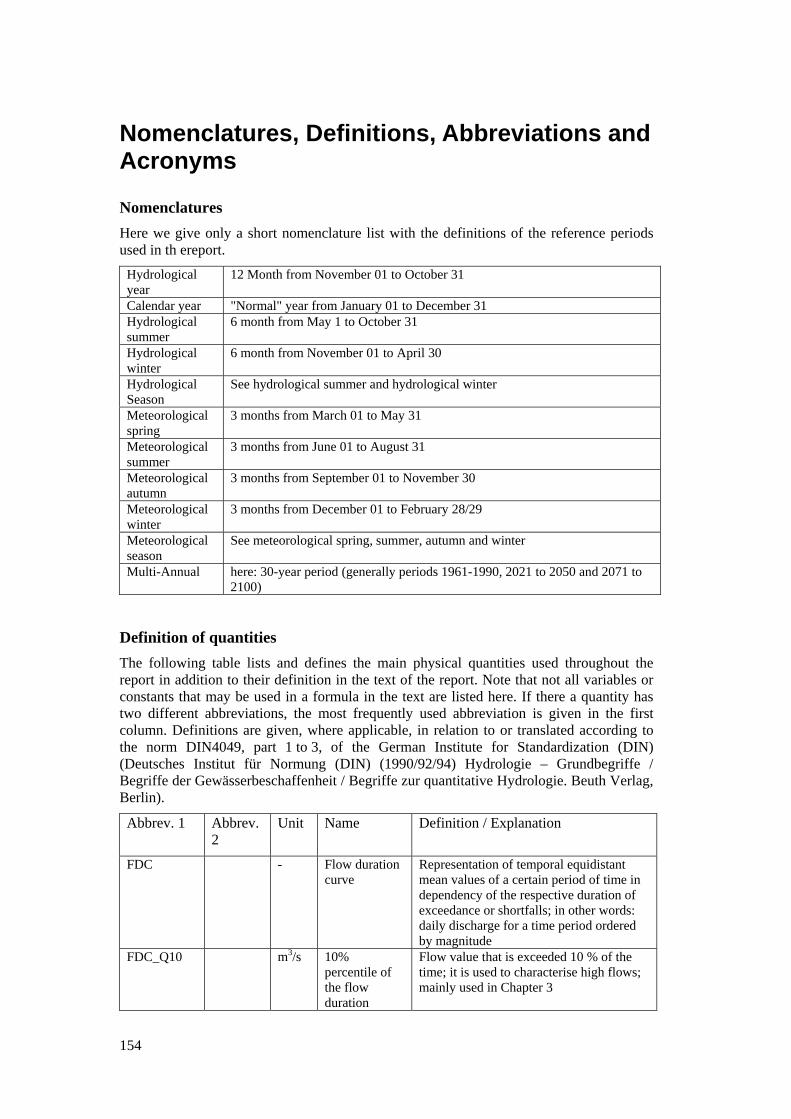
154
Nomenclatures, Definitions, Abbreviations and Acronyms
Nomenclatures Here we give only a short nomenclature list with the definitions of the reference periods used in th ereport.
Hydrological year
12 Month from November 01 to October 31
Calendar year "Normal" year from January 01 to December 31 Hydrological summer
6 month from May 1 to October 31
Hydrological winter
6 month from November 01 to April 30
Hydrological Season
See hydrological summer and hydrological winter
Meteorological spring
3 months from March 01 to May 31
Meteorological summer
3 months from June 01 to August 31
Meteorological autumn
3 months from September 01 to November 30
Meteorological winter
3 months from December 01 to February 28/29
Meteorological season
See meteorological spring, summer, autumn and winter
Multi-Annual here: 30-year period (generally periods 1961-1990, 2021 to 2050 and 2071 to 2100)
Definition of quantities The following table lists and defines the main physical quantities used throughout the report in addition to their definition in the text of the report. Note that not all variables or constants that may be used in a formula in the text are listed here. If there a quantity has two different abbreviations, the most frequently used abbreviation is given in the first column. Definitions are given, where applicable, in relation to or translated according to the norm DIN4049, part 1 to 3, of the German Institute for Standardization (DIN) (Deutsches Institut für Normung (DIN) (1990/92/94) Hydrologie – Grundbegriffe / Begriffe der Gewässerbeschaffenheit / Begriffe zur quantitative Hydrologie. Beuth Verlag, Berlin).
Abbrev. 1 Abbrev. 2
Unit Name Definition / Explanation
FDC - Flow duration curve
Representation of temporal equidistant mean values of a certain period of time in dependency of the respective duration of exceedance or shortfalls; in other words: daily discharge for a time period ordered by magnitude
FDC_Q10 m3/s 10% percentile of the flow duration
Flow value that is exceeded 10 % of the time; it is used to characterise high flows; mainly used in Chapter 3
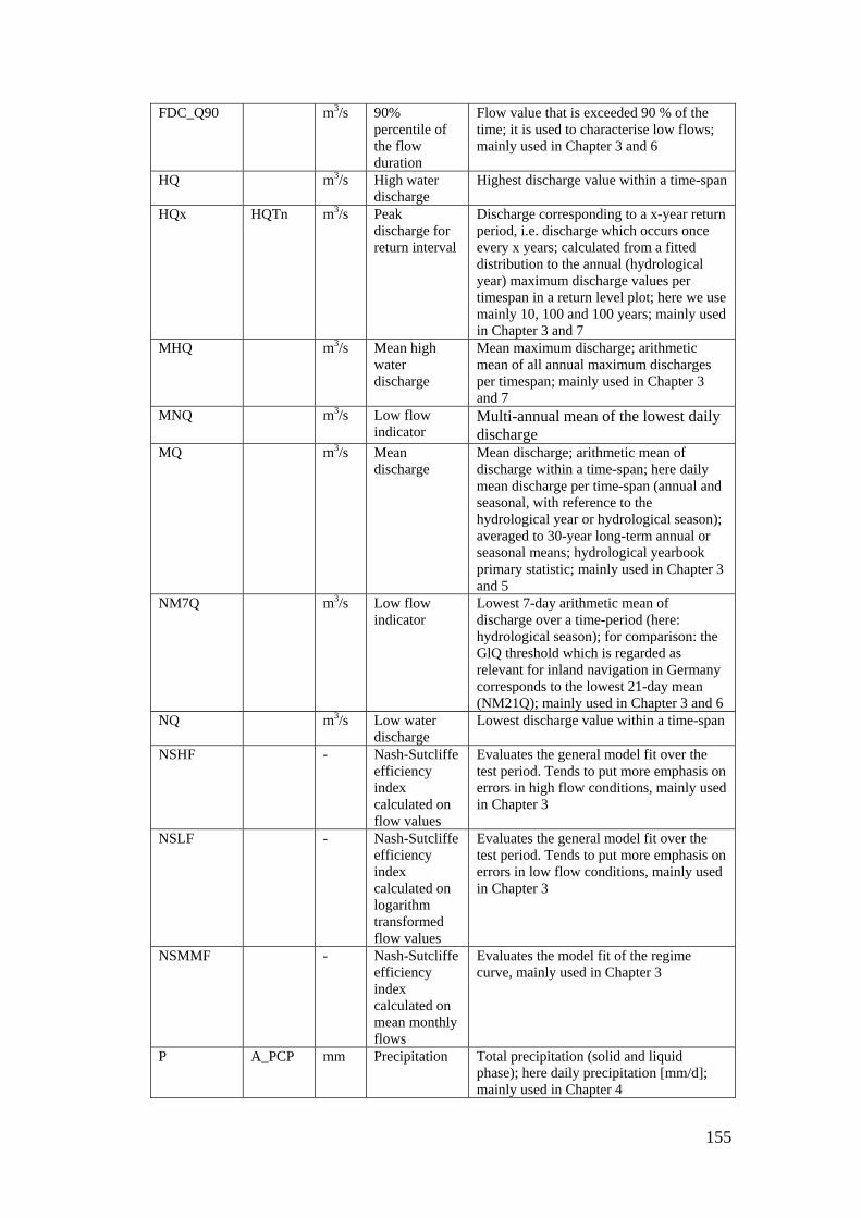
155
FDC_Q90 m3/s 90% percentile of the flow duration
Flow value that is exceeded 90 % of the time; it is used to characterise low flows; mainly used in Chapter 3 and 6
HQ m3/s High water discharge
Highest discharge value within a time-span
HQx HQTn m3/s Peak discharge for return interval
Discharge corresponding to a x-year return period, i.e. discharge which occurs once every x years; calculated from a fitted distribution to the annual (hydrological year) maximum discharge values per timespan in a return level plot; here we use mainly 10, 100 and 100 years; mainly used in Chapter 3 and 7
MHQ m3/s Mean high water discharge
Mean maximum discharge; arithmetic mean of all annual maximum discharges per timespan; mainly used in Chapter 3 and 7
MNQ m3/s Low flow indicator
Multi-annual mean of the lowest daily discharge
MQ m3/s Mean discharge
Mean discharge; arithmetic mean of discharge within a time-span; here daily mean discharge per time-span (annual and seasonal, with reference to the hydrological year or hydrological season); averaged to 30-year long-term annual or seasonal means; hydrological yearbook primary statistic; mainly used in Chapter 3 and 5
NM7Q m3/s Low flow indicator
Lowest 7-day arithmetic mean of discharge over a time-period (here: hydrological season); for comparison: the GlQ threshold which is regarded as relevant for inland navigation in Germany corresponds to the lowest 21-day mean (NM21Q); mainly used in Chapter 3 and 6
NQ m3/s Low water discharge
Lowest discharge value within a time-span
NSHF - Nash-Sutcliffe efficiency index calculated on flow values
Evaluates the general model fit over the test period. Tends to put more emphasis on errors in high flow conditions, mainly used in Chapter 3
NSLF - Nash-Sutcliffe efficiency index calculated on logarithm transformed flow values
Evaluates the general model fit over the test period. Tends to put more emphasis on errors in low flow conditions, mainly used in Chapter 3
NSMMF - Nash-Sutcliffe efficiency index calculated on mean monthly flows
Evaluates the model fit of the regime curve, mainly used in Chapter 3
P A_PCP mm Precipitation Total precipitation (solid and liquid phase); here daily precipitation [mm/d]; mainly used in Chapter 4

156
ETpot PE mm Potential evapo-transpiration
Amount of soil evaporation, interception, and transpiration under given meteorological conditions under the assumption of unlimited water availability; here daily evapotranspiration [mm/d]; mainly used in Chapter 2
Q m3/s Discharge Water volume that flows through a certain profile in a unit of time
RFDC_Q10 - Bias on 10% flow percentile
Ratio between the simulated and observed 10% (exceedance) percentiles of daily flows; evaluates the fit in high flow conditions, mainly used in Chapter 3
RFDC_Q90 - Bias on 90% flow percentile
Ratio between the simulated and observed 90% (exceedance) percentiles of daily flows; evaluates the fit in low flow conditions, mainly used in Chapter 3
RMQ - Overall bias Ratio between the simulated and observed mean flows over the evaluation period.; evaluates the relative volumetric model error, mainly used in Chapter 3
T TMP °C Air temperature 2 m (daily means)
Usually here in 2 m
Abbreviations and Acronyms15 Please note that RCM or GCM are not listed in the table below. The original meaning of an abbreviation or acronym is given first, if a common or official English translastion exist this is given in paraentheses. Project or programme acronyms are in italics.
AS Advanced scaling (bias-correction method) BAFU/FOEN Bundesamt für Umwelt (Federal Office for the Environment), Bern, Switzerland BC Bias-correction method BfG Bundesanstalt für Gewässerkunde (Federal Institute of Hydrology), Koblenz,
Germany CCHydro Klimaänderung und Hydrologie in der Schweiz CDF Cummulative distribution function CERA Climate and Environmental Retrieving and Archiving database (via WDCC, see
below) CEC Climate & Environment Consulting Potsdam GmbH, Potsdam, Germany CLINO Climate normal (time-span) CMIP Coupled Model Intercomparison Project CORDEX COordinated Regional climate Downscaling Experiment CRP-GL Centre de Recherche Public – Gabriel Lippmann (Public Research Centre –
Gabriel Lippmann), Belvaux, Luxembourg DWD Deutscher Wetterdienst (German Weather Service), Offenbach, Germany ETHZ Eidgenössische Technische Hochschule Zürich (Swiss Federal Institute of
Technology Zürich), Zürich, Switzerland EVAP Evaporation approach EOU Evapotranspiration approach after Oudin EPW Evapotranspiration approach after Penman-Wendling HBAN Hydrosystems and Bioprocesses Research Unit HLUG Hessisches Landesamt für Umwelt und Geologie, Wiesbaden, Germany HWRP Hydrological Water Resources Programme GCM Global Climate Model (mostly coupled atmosphere-ocean global climate model,
15 Also explained at their first occurrence in the text.

157
AOGCM) GEV Generalized Extreme Value (distribution) GIS Geographical Information System IHP International Hydrological Programme IKSR (ICPR) Internationale Kommission zum Schutz des Rheins (International Commission
for the Protection of the Rhine), Koblenz, Germany IPCC Intergovernmental Panel on Climate Change KNMI Koninklijk Nederlands Meteorologisch Instituut (Royal Netherlands
Meteorological Institute), De Bilt, The Netherlands KHR (CHR) Internationale Kommission für die Hydrologie des Rheingebietes (International
Commission for the Hydrology of the Rhine Basin) LS Linear scaling (bias-correction mehod) MIUB Meteorological Institute University of Bonn, Germany MPI-M Max-Planck-Institute for Meteorology, Hamburg, Germany OcCC Beratende Organ für Fragen der Klimaänderung (Advisory Body on Climate
Change), Switzerland PIK Potsdam Institut für Klimafolgenforschung (Potsdam Institute for Climate
Impact Research), Potsdam, Germany ProClim- Forum for Climate and Global Change PRUDENCE Prediction of Regional scenarios and Uncertainties for Defining EuropeaN
Climate change risks and Effects RCM Regional climate model RDS Regional downscaling RWS(-WD) Rijkswaterstaat (Rijkswaterstaat Centre for Water Management), Lelystad, The
Netherlands SRES Special Report on Emission Scenarios (GHG emission Scenario based on
Nakicenovic, et al., 2000) sRDS Statistical regional downscaling STARDEX STAtistical and Regional dynamical Downscaling of EXtremes for European
regions TFRCD Task Force on Regional Climate Downscaling UKCP09 United Kingdom Climate Projections ‘09 UNESCO United Nations Educational, Scientific and Cultural Organization WCRP World Climate Research Program WDCC World Data Center for Climate, Hamburg, Germany WBM Water balance model, hydrological model WMO World Meteorological Organisation
158
CHR Publications
CHR/KHR (1978): Das Rheingebiet, Hydrologische Monographie. Staatsuitgeverij, Den Haag / Le bassin du Rhin. Monographie Hydrologique. Staatsuitgeverij, La Haye. ISBN 90-12017-75-0 (no longer available)
Reports of the CHR I-1 GREBNER, D. (1982): Objektive quantitative Niederschlagsvorhersagen im Rheingebiet. Stand 1982 (nicht mehr lieferbar) / Prévisions objectives et quantitatives des précipitations dans le bassin du Rhin. Etat de la question en 1982 (édition épuisée)
I-2 GERHARD, H.; MADE, J.W. VAN DER; REIFF, J.; VREES, L.P.M. DE (1983): Die Trocken- und Niedrigwasserperiode 1976. (2. Auflage 1985) / La sécheresse et les basses eaux de 1976 (2ème édition, 1985). ISBN 90-70980-01-0
I-3 HOFIUS, K. (1985): Hydrologische Untersuchungsgebiete im Rheingebiet / Bassins de recherches hydrologiques dans le bassin du Rhin. ISBN 90-70980-02-9
I-4 BUCK, W.; KIPGEN, R.; MADE, J.W. VAN DER; MONTMOLLIN, F. DE; ZETTL, H.; ZUMSTEIN, J.F. (1986): Berechnung von Hoch- und Niedrigwasserwahrscheinlichkeit im Rheingebiet / Estimation des probabilités de crues et d'étiages dans le bassin du Rhin. ISBN 90-7098003-7
I-5 TEUBER, W.; VERAART, A.J. (1986): Abflußermittlung am Rhein im deutschniederländischen Grenzbereich / La détermination des débits du Rhin dans la région frontalière germano-hollandaise. ISBN 90-70980-04-5
I-6 TEUBER, W. (1987): Einfluß der Kalibrierung hydrometrischer Meßflügel auf die Unsicherheit der Abflußermittlung. Ergebnisse eines Ringversuchs / Influence de l'étalonnage des moulinets hydrométriques sur l'incertitude des déterminations de débits. Résultats d'une étude comparative. ISBN 90-70980-05-3
I-7 MENDEL, H.G. (1988): Beschreibung hydrologischer Vorhersagemodelle im Rheineinzugsgebiet / Description de modèles de prévision hydrologiques dans le bassin du Rhin. ISBN 90-7098006-1
I-8 ENGEL, H.; SCHREIBER, H.; SPREAFICO, M.; TEUBER, W.; ZUMSTEIN, J.F. (1990): Abflußermittlung im Rheingebiet im Bereich der Landesgrenzen / Détermination des débits dans les régions frontalières du bassin du Rhin. ISBN 90-70980-10-x
I-9 CHR/KHR (1990): Das Hochwasser 1988 im Rheingebiet / La crue de 1988 dans le bassin du Rhin. ISBN 90-70980-11-8
I-10 NIPPES, K.R. (1991): Bibliographie des Rheingebietes / Bibliographie du bassin du Rhin. ISBN 90-70980-13-4
I-11 BUCK, W.; FELKEL, K.; GERHARD, H.; KALWEIT, H.; MALDE, J. VAN; NIPPES, K.R.; PLOEGER, B.; SCHMITZ, W. (1993): Der Rhein unter der Einwirkung des Menschen - Ausbau, Schiffahrt, Wasserwirtschaft / Le Rhin sous l'influence de l'homme - Aménagement, navigation, gestion des eaux. ISBN 90-70980-17-7
I-12 SPREAFICO, M.; MAZIJK, A. VAN (Red.). (1993): Alarmmodell Rhein. Ein Modell für die operationelle Vorhersage des Transportes von Schadstoffen im Rhein. ISBN 90-70980-18-5
I-13 SPREAFICO, M.; MAZIJK, A. VAN (réd). (1997): Modèle d'alerte pour le Rhin. Un modèle pour la prévision opérationnelle de le propagation de produits nocifs dans le Rhin. ISBN 9070980-23-1
159
I-14 EMMENEGGER, CH.; et al. (1997): 25 Jahre KHR. Kolloquium aus Anlaß des 25jährigen Bestehens der KHR / 25 ans de la CHR. Colloque à l'occasion du 25e anniversaire de la CHR. 1SBN 90-70980-24-x I-15 ENGEL, H. (1997): Fortschreibung der Monographie des Rheingebietes für die Zeit 1971-1990 / Actualisation de la Monographie du Bassin du Rhin pour la période 1971-1990. ISBN 90-7098025-8
I-16 GRABS, W. (ed.) (1997): Impact of climate change on hydrological regimes and water resources management in the Rhine basin. ISBN 90-70980-26-6
I-17 ENGEL, H. (1999): Eine Hochwasserperiode im Rheingebiet. Extremereignisse zwischen Dez.1993 und Febr. 1995. ISBN 90-70980-28-2
I-18 KOS, Th.J.M.; SCHEMMER, H; JAKOB, A. (2000): Feststoffmessungen zum Vergleich von Messgeräten und Messmethoden im Rhein, 10-12 März 1998. ISBN 90-36953-54-5
I-19 BARBEN, M.; et al. (2001): Übersicht über Verfahren zur Abschätzung von Hochwasserabflüssen – Erfahrungen aus den Rheinanliegerstaaten. ISBN 90-36954-11-8
I-20 KRAHE, P.; HERPERTZ, D. (2001): Generation of Hydrometeorological Reference Conditions for the Assessment of Flood Hazard in large River Basins - Papers presented at the International Workshop held on March 6 and 7, 2001 in Koblenz. ISBN 90-36954-18-5
I-21 KRAHE, P et al.; (2004): Entwicklung einer Methodik zur Analyse des Einflusses dezentraler Hochwasserrückhaltemaßnahmen auf den Abfluss des Rheins.ISBN90-36956-74-9
I-22 BELZ, J.U. et al. (2007): Das Abflussregime des Rheins und seiner Nebenflüsse im 20. Jahrhundert - Analyse, Veränderungen, Trends. ISBN 978-90-70980-33-7
I-23 GÖRGEN, K. et al. (2010): Assessment of Climate Change Impacts on Discharge in the Rhine River Basin: Results of the RheinBlick2050 project. ISBN 978-90-70980-35-1
Katalog/Catalogue 1 SPROKKEREEF, E. (1989): Verzeichnis der für internationale Organisationen wichtigen Meßstellen im Rheingebiet / Tableau de stations de mesure importantes pour les organismes internationaux dans le bassin du Rhin. ISBN 90-70980-08-8.
Reports under the auspices of the CHR II-1 MADE, J.W. VAN DER (1982): Quantitative Analyse der Abflüsse (nicht mehr lieferbar) / Analyse quantitative des débits (édition épuisée)
II-2 GRIFFIOEN, P.S. (l 989): Alarmmodell für den Rhein / Modèle d'alerte pour le Rhin. ISBN 9070980-07-x
II-3 SCHRÖDER, U. (1990): Die Hochwasser an Rhein und Mosel im April und Mai 1983 / Les crues sur les bassins du Rhin et de la Moselle en avril et mai 1983. ISBN 90-70980-09-6
II-4 MAZIJK, A. VAN; VERWOERDT, P.; MIERLO, J. VAN, BREMICKER, M.,WIESNER, H.; (1991): Rheinalarmmodell Version 2.0 - Kalibrierung und Verifikation / Modèle d'alerte pour le Rhin version 2.0 - Calibration et vérification. ISBN 90-70980-12-6
II-5 MADE, J.W. VAN DER; (1991): Kosten-Nutzen-Analyse für den Entwurf hydrometrischer Meßnetze / Analyse des coûts et des bénéfices pour le projet d'un réseau hydrométrique. ISBN 9070980-14-2
II-6 CHR/KHR (1992): Contributions to the European workshop Ecological Rehabilitation of Floodplains, Arnhem, The Netherlands, 22-24 September 1992. ISBN 90-70980-15-0
160
II-7 NEMEC, J. (1993): Comparison and selection of existing hydrological models for the simulation of the dynamic water balance processes in basins of different sizes and on different scales. ISBN 90-70980-16-9
II-8 MENDEL, H.G. (1993): Verteilungsfunktionen in der Hydrologie. ISBN 90-70980-19-3
II-9 WITTE, W.; KRAHE, P.; LIEBSCHER, H.J. (1995): Rekonstruktion der Witterungsverhältnisse im Mittelrheingebiet von 1000 n. Chr. bis heute anhand historischer hydrologischer Ereignisse. ISBN 90-70980-20-7
II-10 WILDENHAHN, E,; KLAHOLZ, U. (1996): Grobe Speicherseen im Einzugsgebiet des Rheins. ISBN 90-70980-21-5
II-11 SPREAFICO, M.; LEHMANN, C.; SCHEMMER, H.; BURGDOR-FFER, M.; KOS, T.L. (1996): Feststoffbeobachtung im Rhein, Beschreibung der Meßgeräte und Meßmethoden. ISBN 90-70980-22-3
II-12 SCHÂDLER, B. (Red.) (1997): Bestandsaufnahme der Meldesysteme und Vorschläge zur Verbesserung der Hochwasservorhersage im Rheingebiet. Schlußbericht der IKSR-Arbeitseinheit 'Meldesysteme / Hochwasservorhersage' - Projektgruppe 'Aktionsplan Hochwasser' / Annonce et prévision des crues dans le bassin du Rhin. Etat actuel et propositions d'amélioration. Rapport final de l'unité de travail 'Systèmes d'annonce / prévision des crues' - Groupe de projet 'Plan d'action contre les inondations'. ISBN 90-70980-27-4
II-13 DRÖGE, B.; HENOCH, H.; KELBER, W.; MAHR, U.; SWANENBERG, T.;, THIELEMANN, T.; THURM, U. (1999): Entwicklung eines Längsprofils des Rheins. Bericht für die Musterstrecke von Rhein-km 800 - 845. Arbeitsgruppe 'Sedimenttransport im Rhein' Projekt 3. ISBN 90-70980-29-0
II-14 MAZIJK, A.. VAN; LEIBUNDGUT, CH.; NEFF, H.P. (1999): Rhein-Alarm-Modell Version 2. 1. Erweiterung um die Kalibrierung von Aare und Mosel. Kalibrierungsergebnisse von Aare und Mosel aufgrund der Markierversuche 05/92, 11/92 und 03/94. ISBN 90-70980-30-4
II-15 KWADIJK, J.; DEURSEN, W. VAN (1999): Development and testing of a GIS based water balance model for the Rhine drainage basin. ISBN 90-70980-31-2
II-16 MAZIJK, A.. VAN;, GILS, J.A.G. VAN; WEITBRECHT, V.; VOLLSTEDT, S. (2000): ANALYSE und EVALUIERUNG der 2D-MODULE zur Berechnung des Stofftransportes in der Windows-Version des RHEINALARMMODELLS in Theorie und Praxis. ISBN 90-36953-55-3
II-17 SPREAFICO, M.; WEINGARTNER, R, et al; (2002): Proceedings International Conference on Flood Estimation, March, 6-8, 2002 Berne, Switzerland. ISBN 90-36954-60-6
II-18 BRONSTERT, A, et al; (2003): LAHoR – Quantifizierung des Einflusses der Landoberfläche und der Ausbaumassnahmen am Gewässer auf die Hochwasserbedingungen im Rheingebiet. ISBN 90-70980-32-0
II-19 KROEKENSTOEL, D.F.; VELZEN, E.H. VAN (2003): Morphologische Berechnungen mit Sedimentmischungen – Zukunftmusik oder eine realistische Alternative? ISBN 90-36954-98-3
II-20 SPREAFICO, M.; LEHMANN, Ch. (Ed.) (2009): Erosion, Transport an Deposition of Sediment - Case Study Rhine. Contribution to the International Sediment Initiative of UNESCO/IHP. ISBN 978-90-70980-34-4

161
Appendix
A Target Measures
B Regional Climate Change Projections Data Overview
C Hydrological Model Features
D Performance of Hydrological Models
E Air Temperature and Precipitation Changes
F Extreme Value Analyses of Simulated Discharges
G Flood Statistics Provided by the German Federal States and Rijkswaterstaat
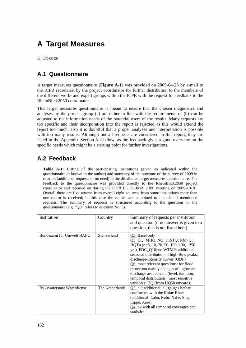
162
A Target Measures
K. GÖRGEN
A.1 Questionnaire
A target measures questionnaire (Figure A-1) was provided on 2009-04-23 by e-mail to the ICPR secretariat by the project coordinator for further distribution to the members of the different work- and expert groups within the ICPR with the request for feedback to the RheinBlick2050 coordinator.
This target measures questionnaire is meant to ensure that the chosen diagnostics and analyses by the project group (a) are either in line with the requirements or (b) can be adjusted to the information needs of the potential users of the results. Many requests are too specific and their incorporation into the report is rejected as this would extend the report too much; also it is doubtful that a proper analyses and interpretation is possible with too many results. Although not all requests are considered in this report, they are listed in the Appendix Section A.2 below, as the feedback gives a good overview on the specific needs which might be a starting point for further investigations.
A.2 Feedback Table A-1: Listing of the participating institutions (given as indicated within the questionnaire or known to the author) and summary of the outcome of the survey of 2009 in relation (additional requests or no need) to the distributed target measures questionnaire. The feedback to the questionnaire was provided directly to the RheinBlick2050 project coordinator and reported on during the ICPR EG KLIMA 2(09) meeting on 2009-10-20. Overall there are five returns from overall eight sources; from some institutions more than one return is received; in this case the replies are combined to include all mentioned requests. The summary of requests is structured according to the questions in the questionnaire (e.g. “Q3” refers to question No. 3).
Institution Country Summary of requests per institution and question (if no answer is given to a question, this is not listed here)
Bundesamt für Umwelt BAFU Switzerland Q3: Basel only Q5: HQ, MHQ, NQ; DISTQ; NM7Q; HQTn (n=5, 10, 20, 50, 100, 200, 1250 yrs), FDC_Q10; no WTMP; additional: seasonal distribution of high-flow peaks, discharge-intensity curves (QDF) Q6: most relevant questions: for flood protection mainly changes of highwater discharge are relevant (level, duration, temporal distribution); most sensitive variables: HQ (from HQ50 onwards)
Rijkswaterstaat Waterdienst The Netherlands Q3: all; additional: all gauges before confluence with the Rhine River (additional: Lahn, Ruhr, Nahe, Sieg, Lippe, Aare) Q4: ok with all temporal coverages and statistics
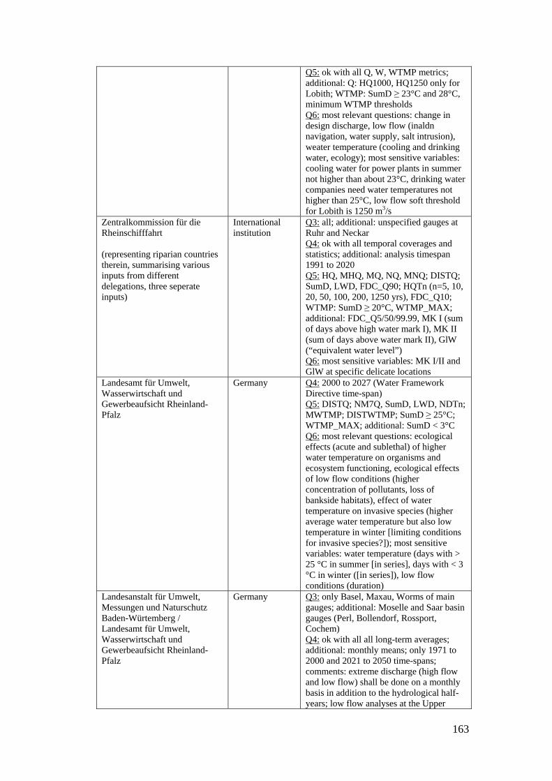
163
Q5: ok with all Q, W, WTMP metrics; additional: Q: HQ1000, HQ1250 only for Lobith; WTMP: SumD ≥ 23°C and 28°C, minimum WTMP thresholds Q6: most relevant questions: change in design discharge, low flow (inaldn navigation, water supply, salt intrusion), weater temperature (cooling and drinking water, ecology); most sensitive variables: cooling water for power plants in summer not higher than about 23°C, drinking water companies need water temperatures not higher than 25°C, low flow soft threshold for Lobith is 1250 m3/s
Zentralkommission für die Rheinschifffahrt (representing riparian countries therein, summarising various inputs from different delegations, three seperate inputs)
International institution
Q3: all; additional: unspecified gauges at Ruhr and Neckar Q4: ok with all temporal coverages and statistics; additional: analysis timespan 1991 to 2020 Q5: HQ, MHQ, MQ, NQ, MNQ; DISTQ; SumD, LWD, FDC_Q90; HQTn (n=5, 10, 20, 50, 100, 200, 1250 yrs), FDC_Q10; WTMP: SumD ≥ 20°C, WTMP_MAX; additional: FDC_Q5/50/99.99, MK I (sum of days above high water mark I), MK II (sum of days above water mark II), GlW (“equivalent water level”) Q6: most sensitive variables: MK I/II and GlW at specific delicate locations
Landesamt für Umwelt, Wasserwirtschaft und Gewerbeaufsicht Rheinland-Pfalz
Germany Q4: 2000 to 2027 (Water Framework Directive time-span) Q5: DISTQ; NM7Q, SumD, LWD, NDTn; MWTMP; DISTWTMP; SumD ≥ 25°C; WTMP_MAX; additional: SumD < 3°C Q6: most relevant questions: ecological effects (acute and sublethal) of higher water temperature on organisms and ecosystem functioning, ecological effects of low flow conditions (higher concentration of pollutants, loss of bankside habitats), effect of water temperature on invasive species (higher average water temperature but also low temperature in winter [limiting conditions for invasive species?]); most sensitive variables: water temperature (days with > 25 °C in summer [in series], days with < 3 °C in winter ([in series]), low flow conditions (duration)
Landesanstalt für Umwelt, Messungen und Naturschutz Baden-Würtemberg / Landesamt für Umwelt, Wasserwirtschaft und Gewerbeaufsicht Rheinland-Pfalz
Germany Q3: only Basel, Maxau, Worms of main gauges; additional: Moselle and Saar basin gauges (Perl, Bollendorf, Rossport, Cochem) Q4: ok with all all long-term averages; additional: monthly means; only 1971 to 2000 and 2021 to 2050 time-spans; comments: extreme discharge (high flow and low flow) shall be done on a monthly basis in addition to the hydrological half-years; low flow analyses at the Upper
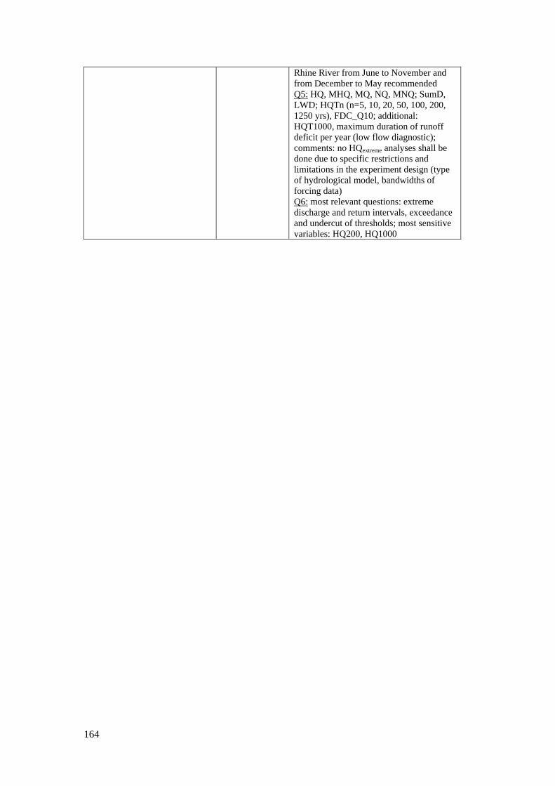
164
Rhine River from June to November and from December to May recommended Q5: HQ, MHQ, MQ, NQ, MNQ; SumD, LWD; HQTn (n=5, 10, 20, 50, 100, 200, 1250 yrs), FDC_Q10; additional: HQT1000, maximum duration of runoff deficit per year (low flow diagnostic); comments: no HQextreme analyses shall be done due to specific restrictions and limitations in the experiment design (type of hydrological model, bandwidths of forcing data) Q6: most relevant questions: extreme discharge and return intervals, exceedance and undercut of thresholds; most sensitive variables: HQ200, HQ1000
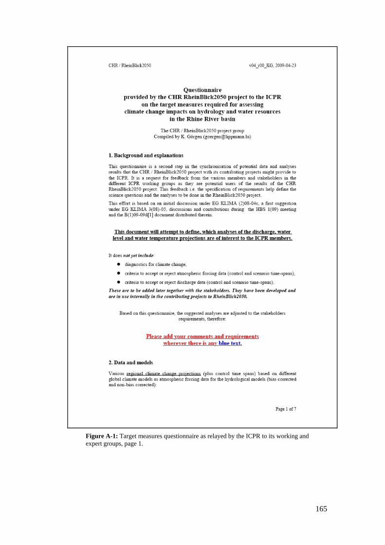
165
Figure A-1: Target measures questionnaire as relayed by the ICPR to its working and expert groups, page 1.
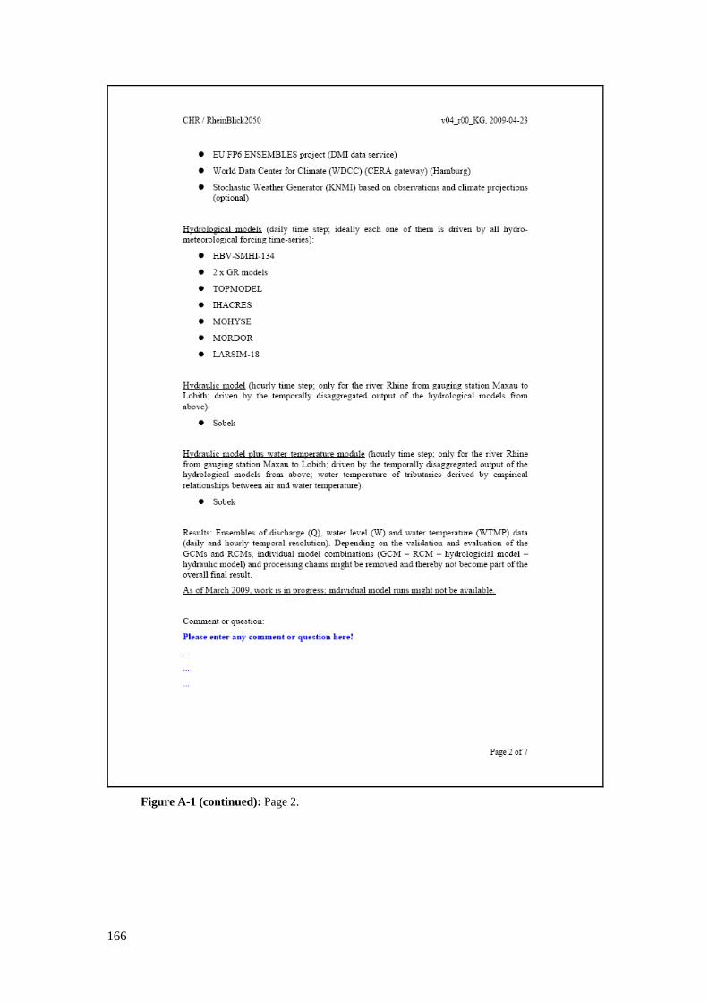
166
Figure A-1 (continued): Page 2.
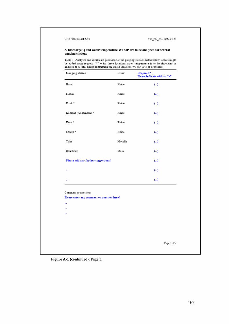
167
Figure A-1 (continued): Page 3.
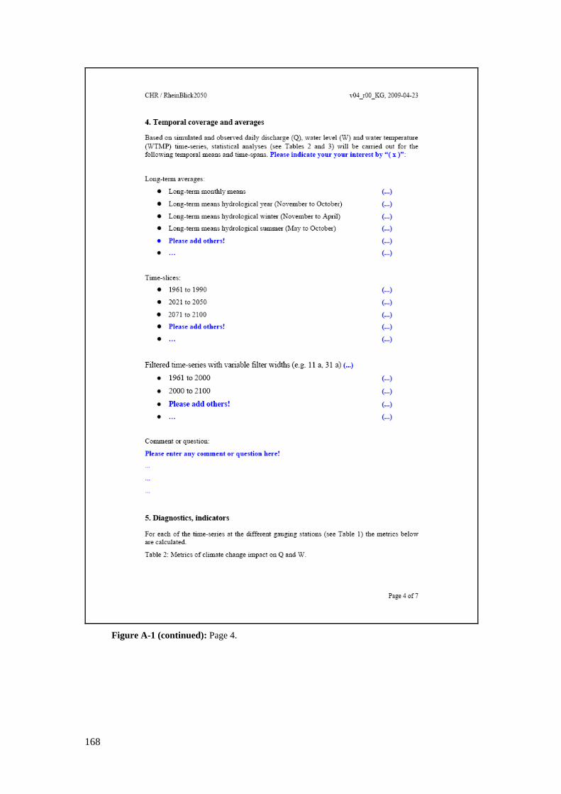
168
Figure A-1 (continued): Page 4.
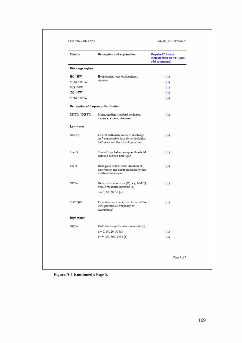
169
Figure A-1 (continued): Page 5.
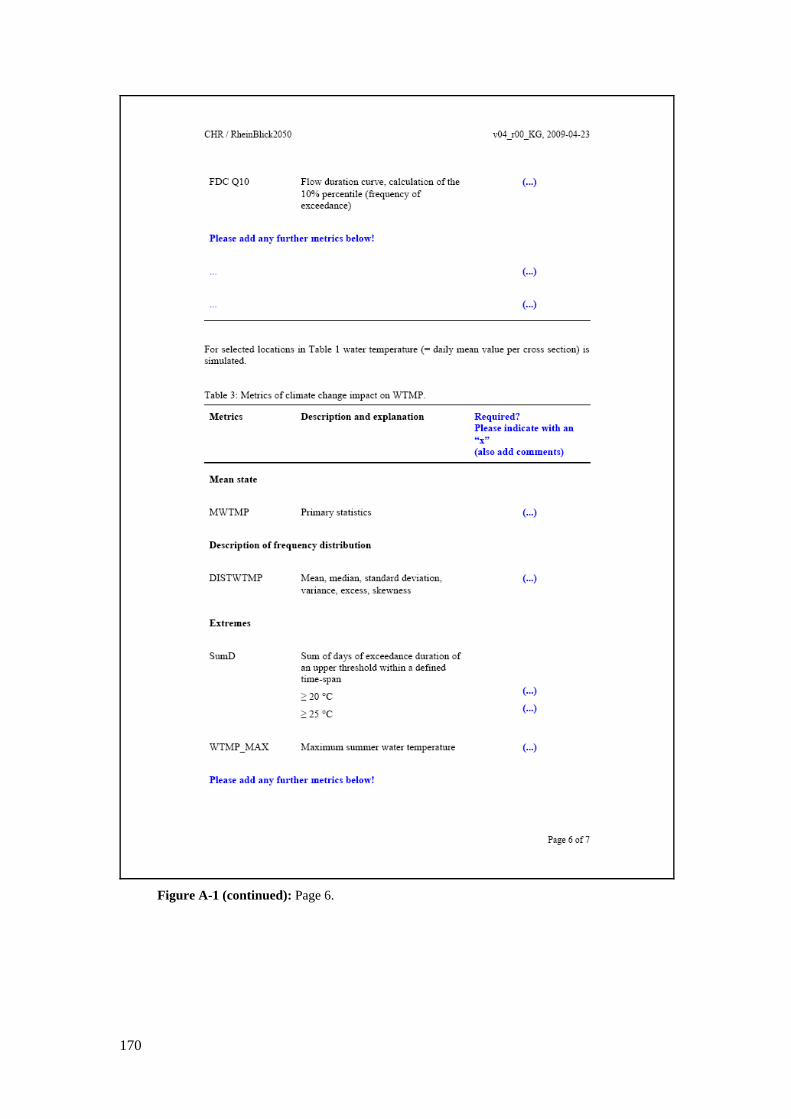
170
Figure A-1 (continued): Page 6.

171
Figure A-1 (continued): Page 7.
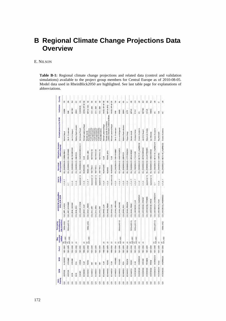
172
B Regional Climate Change Projections Data Overview
E. NILSON
Table B-1: Regional climate change projections and related data (control and validation simulations) available to the project group members for Central Europe as of 2010-08-05. Model data used in RheinBlick2050 are highlighted. See last table page for explanations of abbreviations.
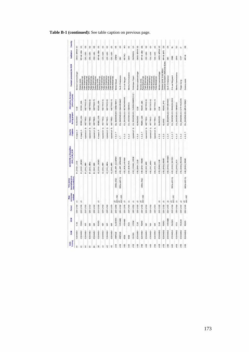
173
Table B-1 (continued): See table caption on previous page.
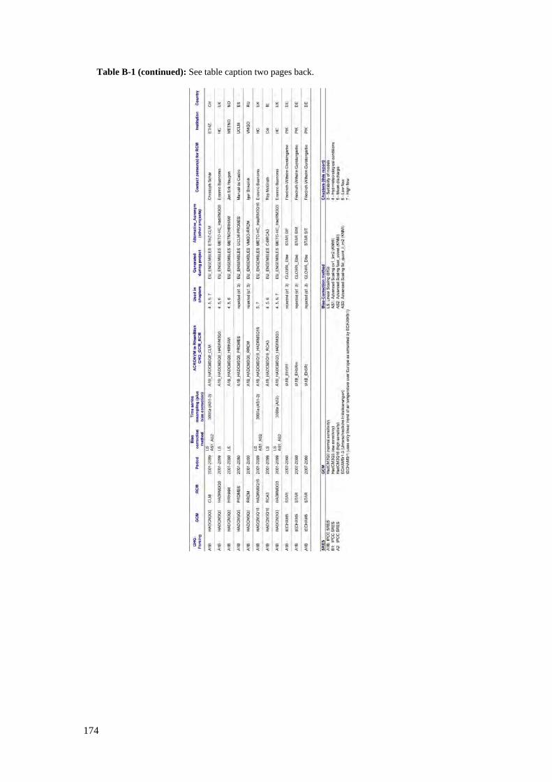
174
Table B-1 (continued): See table caption two pages back.
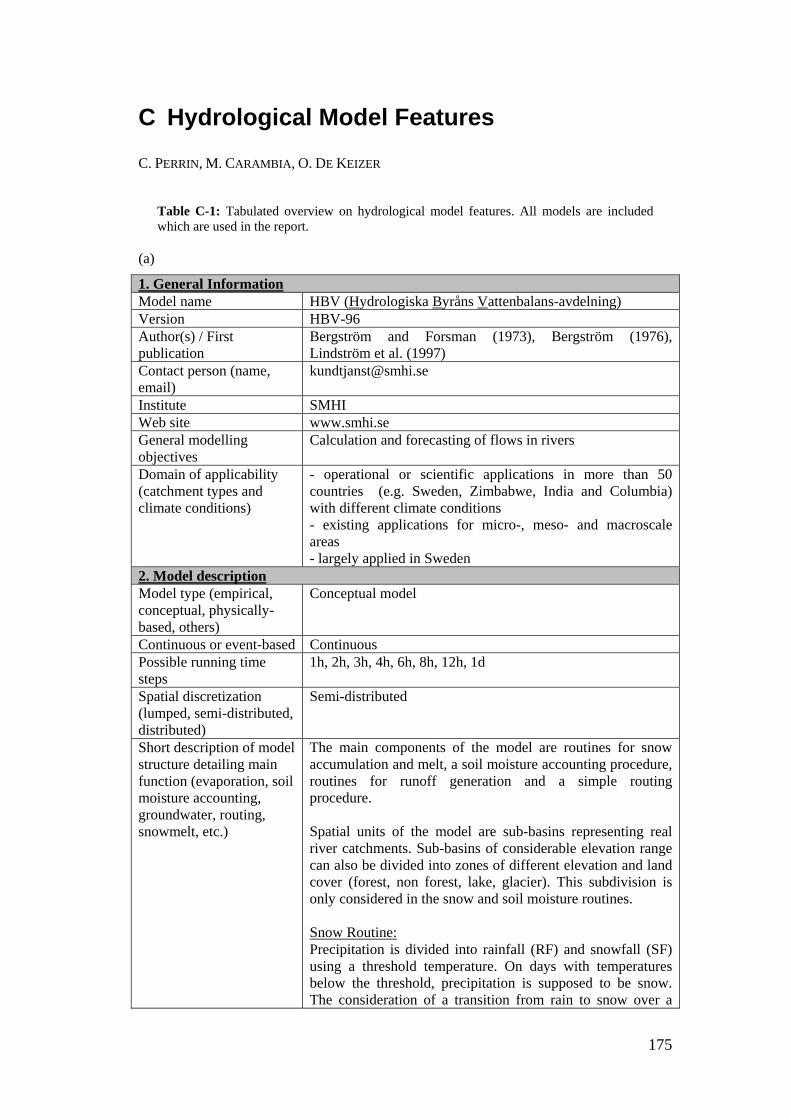
175
C Hydrological Model Features
C. PERRIN, M. CARAMBIA, O. DE KEIZER
Table C-1: Tabulated overview on hydrological model features. All models are included which are used in the report.
(a)
1. General Information Model name HBV (Hydrologiska Byråns Vattenbalans-avdelning) Version HBV-96 Author(s) / First publication
Bergström and Forsman (1973), Bergström (1976), Lindström et al. (1997)
Contact person (name, email)
Institute SMHI Web site www.smhi.se General modelling objectives
Calculation and forecasting of flows in rivers
Domain of applicability (catchment types and climate conditions)
- operational or scientific applications in more than 50 countries (e.g. Sweden, Zimbabwe, India and Columbia) with different climate conditions - existing applications for micro-, meso- and macroscale areas - largely applied in Sweden
2. Model description Model type (empirical, conceptual, physically-based, others)
Conceptual model
Continuous or event-based Continuous Possible running time steps
1h, 2h, 3h, 4h, 6h, 8h, 12h, 1d
Spatial discretization (lumped, semi-distributed, distributed)
Semi-distributed
Short description of model structure detailing main function (evaporation, soil moisture accounting, groundwater, routing, snowmelt, etc.)
The main components of the model are routines for snow accumulation and melt, a soil moisture accounting procedure, routines for runoff generation and a simple routing procedure. Spatial units of the model are sub-basins representing real river catchments. Sub-basins of considerable elevation range can also be divided into zones of different elevation and land cover (forest, non forest, lake, glacier). This subdivision is only considered in the snow and soil moisture routines. Snow Routine: Precipitation is divided into rainfall (RF) and snowfall (SF) using a threshold temperature. On days with temperatures below the threshold, precipitation is supposed to be snow. The consideration of a transition from rain to snow over a
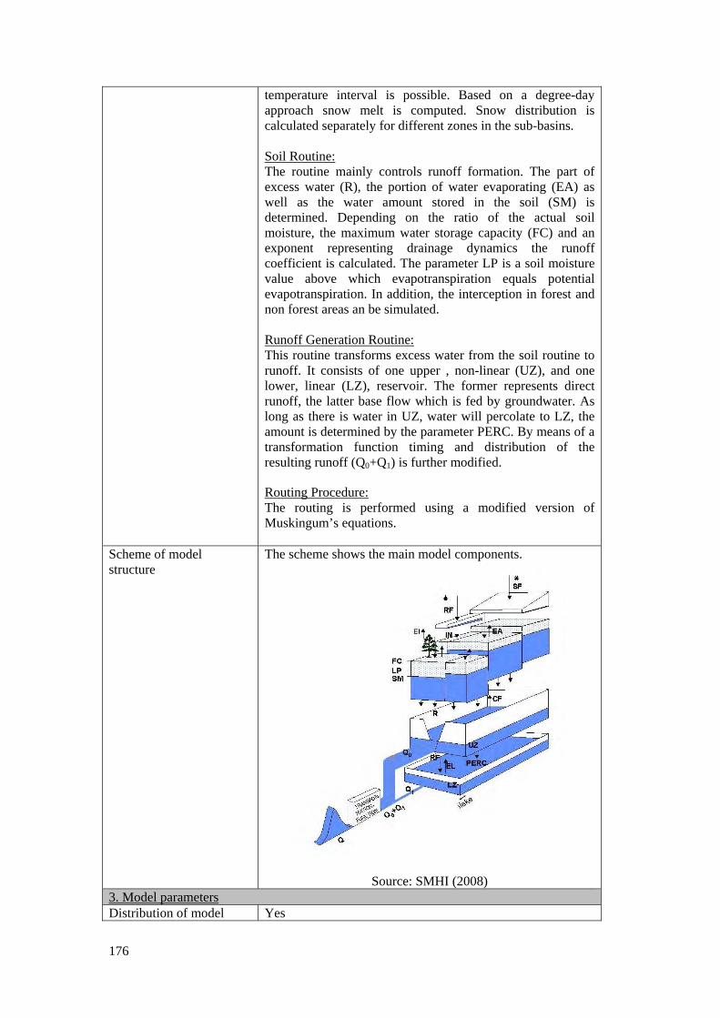
176
temperature interval is possible. Based on a degree-day approach snow melt is computed. Snow distribution is calculated separately for different zones in the sub-basins. Soil Routine: The routine mainly controls runoff formation. The part of excess water (R), the portion of water evaporating (EA) as well as the water amount stored in the soil (SM) is determined. Depending on the ratio of the actual soil moisture, the maximum water storage capacity (FC) and an exponent representing drainage dynamics the runoff coefficient is calculated. The parameter LP is a soil moisture value above which evapotranspiration equals potential evapotranspiration. In addition, the interception in forest and non forest areas an be simulated. Runoff Generation Routine: This routine transforms excess water from the soil routine to runoff. It consists of one upper , non-linear (UZ), and one lower, linear (LZ), reservoir. The former represents direct runoff, the latter base flow which is fed by groundwater. As long as there is water in UZ, water will percolate to LZ, the amount is determined by the parameter PERC. By means of a transformation function timing and distribution of the resulting runoff (Q0+Q1) is further modified. Routing Procedure: The routing is performed using a modified version of Muskingum’s equations.
Scheme of model structure
The scheme shows the main model components.
Source: SMHI (2008) 3. Model parameters Distribution of model Yes
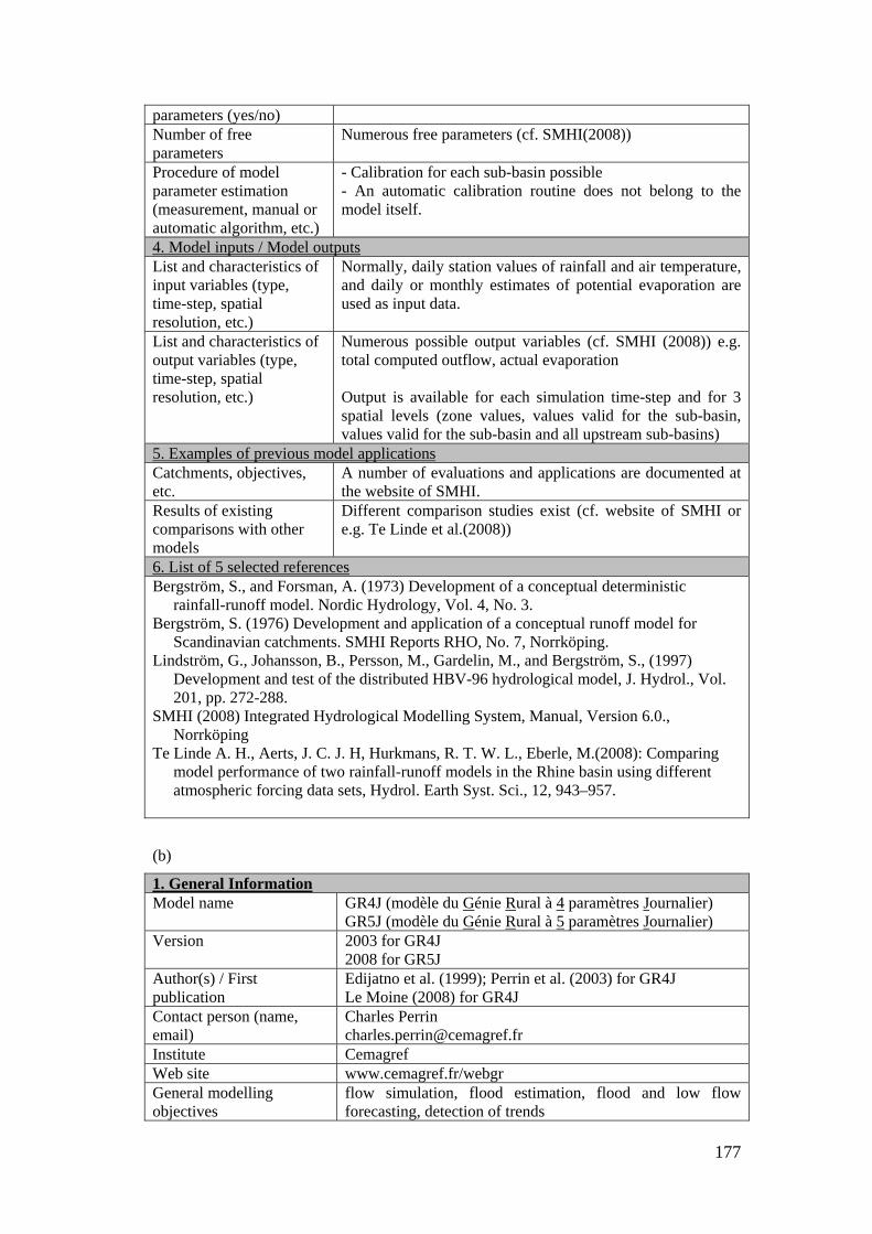
177
parameters (yes/no) Number of free parameters
Numerous free parameters (cf. SMHI(2008))
Procedure of model parameter estimation (measurement, manual or automatic algorithm, etc.)
- Calibration for each sub-basin possible - An automatic calibration routine does not belong to the model itself.
4. Model inputs / Model outputs List and characteristics of input variables (type, time-step, spatial resolution, etc.)
Normally, daily station values of rainfall and air temperature, and daily or monthly estimates of potential evaporation are used as input data.
List and characteristics of output variables (type, time-step, spatial resolution, etc.)
Numerous possible output variables (cf. SMHI (2008)) e.g. total computed outflow, actual evaporation Output is available for each simulation time-step and for 3 spatial levels (zone values, values valid for the sub-basin, values valid for the sub-basin and all upstream sub-basins)
5. Examples of previous model applications Catchments, objectives, etc.
A number of evaluations and applications are documented at the website of SMHI.
Results of existing comparisons with other models
Different comparison studies exist (cf. website of SMHI or e.g. Te Linde et al.(2008))
6. List of 5 selected references Bergström, S., and Forsman, A. (1973) Development of a conceptual deterministic
rainfall-runoff model. Nordic Hydrology, Vol. 4, No. 3. Bergström, S. (1976) Development and application of a conceptual runoff model for
Scandinavian catchments. SMHI Reports RHO, No. 7, Norrköping. Lindström, G., Johansson, B., Persson, M., Gardelin, M., and Bergström, S., (1997)
Development and test of the distributed HBV-96 hydrological model, J. Hydrol., Vol. 201, pp. 272-288.
SMHI (2008) Integrated Hydrological Modelling System, Manual, Version 6.0., Norrköping
Te Linde A. H., Aerts, J. C. J. H, Hurkmans, R. T. W. L., Eberle, M.(2008): Comparing model performance of two rainfall-runoff models in the Rhine basin using different atmospheric forcing data sets, Hydrol. Earth Syst. Sci., 12, 943–957.
(b)
1. General Information Model name GR4J (modèle du Génie Rural à 4 paramètres Journalier)
GR5J (modèle du Génie Rural à 5 paramètres Journalier) Version 2003 for GR4J
2008 for GR5J Author(s) / First publication
Edijatno et al. (1999); Perrin et al. (2003) for GR4J Le Moine (2008) for GR4J
Contact person (name, email)
Charles Perrin [email protected]
Institute Cemagref Web site www.cemagref.fr/webgr General modelling objectives
flow simulation, flood estimation, flood and low flow forecasting, detection of trends
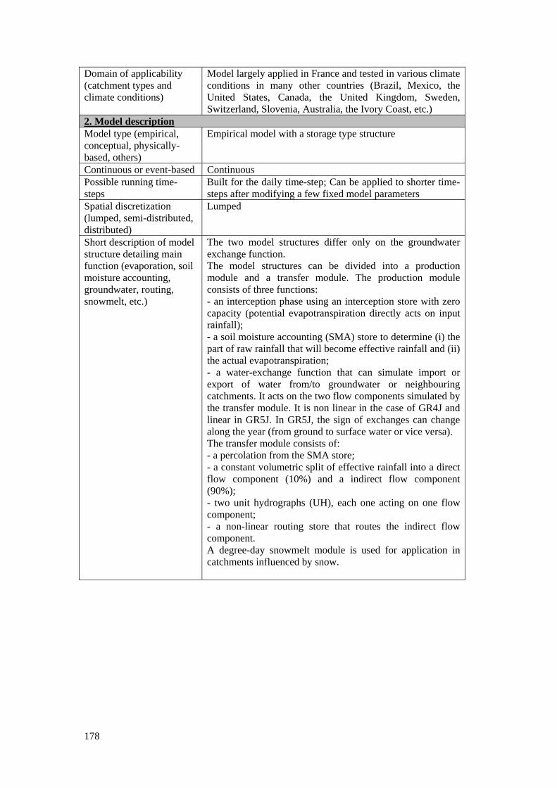
178
Domain of applicability (catchment types and climate conditions)
Model largely applied in France and tested in various climate conditions in many other countries (Brazil, Mexico, the United States, Canada, the United Kingdom, Sweden, Switzerland, Slovenia, Australia, the Ivory Coast, etc.)
2. Model description Model type (empirical, conceptual, physically-based, others)
Empirical model with a storage type structure
Continuous or event-based Continuous Possible running time-steps
Built for the daily time-step; Can be applied to shorter time-steps after modifying a few fixed model parameters
Spatial discretization (lumped, semi-distributed, distributed)
Lumped
Short description of model structure detailing main function (evaporation, soil moisture accounting, groundwater, routing, snowmelt, etc.)
The two model structures differ only on the groundwater exchange function. The model structures can be divided into a production module and a transfer module. The production module consists of three functions: - an interception phase using an interception store with zero capacity (potential evapotranspiration directly acts on input rainfall); - a soil moisture accounting (SMA) store to determine (i) the part of raw rainfall that will become effective rainfall and (ii) the actual evapotranspiration; - a water-exchange function that can simulate import or export of water from/to groundwater or neighbouring catchments. It acts on the two flow components simulated by the transfer module. It is non linear in the case of GR4J and linear in GR5J. In GR5J, the sign of exchanges can change along the year (from ground to surface water or vice versa). The transfer module consists of: - a percolation from the SMA store; - a constant volumetric split of effective rainfall into a direct flow component (10%) and a indirect flow component (90%); - two unit hydrographs (UH), each one acting on one flow component; - a non-linear routing store that routes the indirect flow component. A degree-day snowmelt module is used for application in catchments influenced by snow.
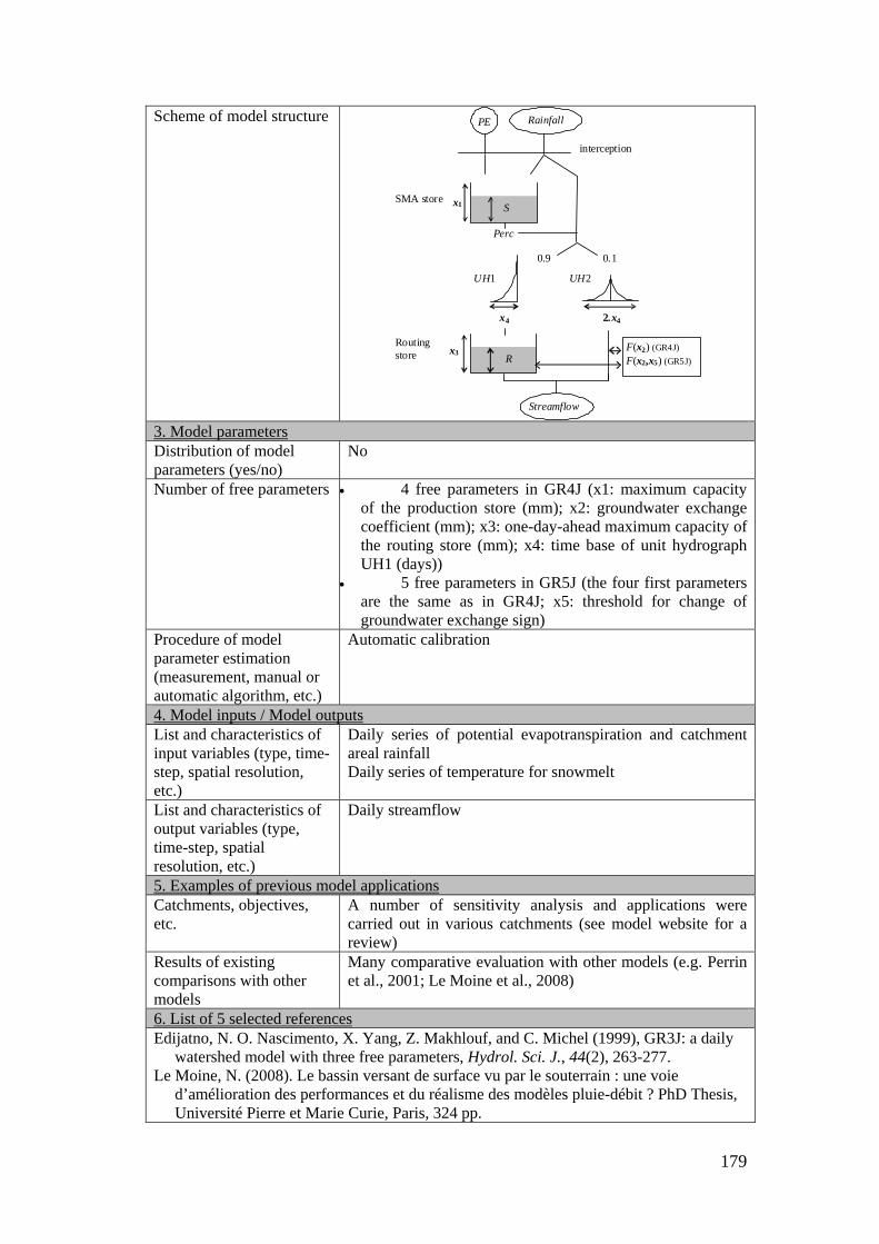
179
Scheme of model structure
PE Rainfall
interception
0.9 0.1
UH1 UH2
Streamflow
x1
x3
S
R
Perc
SMA store
Routing store
2.x4x4
F(x2) (GR4J) F(x2,x5) (GR5J)
3. Model parameters Distribution of model parameters (yes/no)
No
Number of free parameters • 4 free parameters in GR4J (x1: maximum capacity of the production store (mm); x2: groundwater exchange coefficient (mm); x3: one-day-ahead maximum capacity of the routing store (mm); x4: time base of unit hydrograph UH1 (days))
• 5 free parameters in GR5J (the four first parameters are the same as in GR4J; x5: threshold for change of groundwater exchange sign)
Procedure of model parameter estimation (measurement, manual or automatic algorithm, etc.)
Automatic calibration
4. Model inputs / Model outputs List and characteristics of input variables (type, time-step, spatial resolution, etc.)
Daily series of potential evapotranspiration and catchment areal rainfall Daily series of temperature for snowmelt
List and characteristics of output variables (type, time-step, spatial resolution, etc.)
Daily streamflow
5. Examples of previous model applications Catchments, objectives, etc.
A number of sensitivity analysis and applications were carried out in various catchments (see model website for a review)
Results of existing comparisons with other models
Many comparative evaluation with other models (e.g. Perrin et al., 2001; Le Moine et al., 2008)
6. List of 5 selected references Edijatno, N. O. Nascimento, X. Yang, Z. Makhlouf, and C. Michel (1999), GR3J: a daily
watershed model with three free parameters, Hydrol. Sci. J., 44(2), 263-277. Le Moine, N. (2008). Le bassin versant de surface vu par le souterrain : une voie
d’amélioration des performances et du réalisme des modèles pluie-débit ? PhD Thesis, Université Pierre et Marie Curie, Paris, 324 pp.
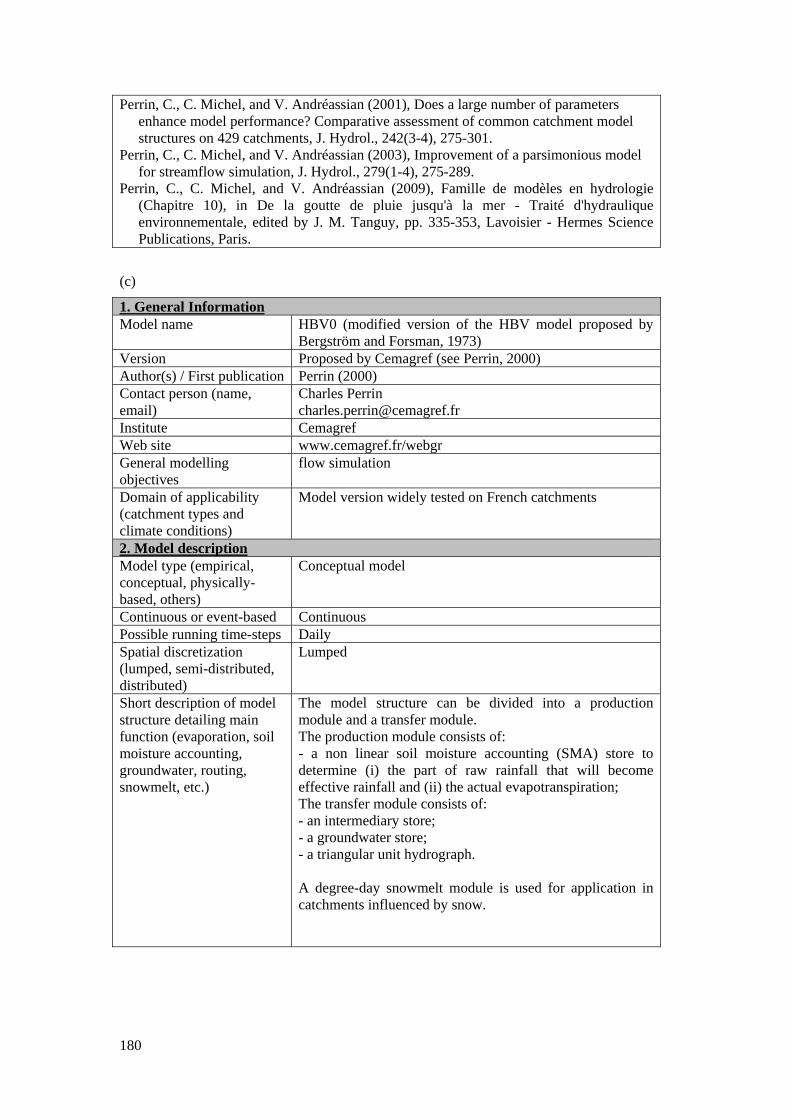
180
Perrin, C., C. Michel, and V. Andréassian (2001), Does a large number of parameters enhance model performance? Comparative assessment of common catchment model structures on 429 catchments, J. Hydrol., 242(3-4), 275-301.
Perrin, C., C. Michel, and V. Andréassian (2003), Improvement of a parsimonious model for streamflow simulation, J. Hydrol., 279(1-4), 275-289.
Perrin, C., C. Michel, and V. Andréassian (2009), Famille de modèles en hydrologie (Chapitre 10), in De la goutte de pluie jusqu'à la mer - Traité d'hydraulique environnementale, edited by J. M. Tanguy, pp. 335-353, Lavoisier - Hermes Science Publications, Paris.
(c)
1. General Information Model name HBV0 (modified version of the HBV model proposed by
Bergström and Forsman, 1973) Version Proposed by Cemagref (see Perrin, 2000) Author(s) / First publication Perrin (2000) Contact person (name, email)
Charles Perrin [email protected]
Institute Cemagref Web site www.cemagref.fr/webgr General modelling objectives
flow simulation
Domain of applicability (catchment types and climate conditions)
Model version widely tested on French catchments
2. Model description Model type (empirical, conceptual, physically-based, others)
Conceptual model
Continuous or event-based Continuous Possible running time-steps Daily Spatial discretization (lumped, semi-distributed, distributed)
Lumped
Short description of model structure detailing main function (evaporation, soil moisture accounting, groundwater, routing, snowmelt, etc.)
The model structure can be divided into a production module and a transfer module. The production module consists of: - a non linear soil moisture accounting (SMA) store to determine (i) the part of raw rainfall that will become effective rainfall and (ii) the actual evapotranspiration; The transfer module consists of: - an intermediary store; - a groundwater store; - a triangular unit hydrograph. A degree-day snowmelt module is used for application in catchments influenced by snow.
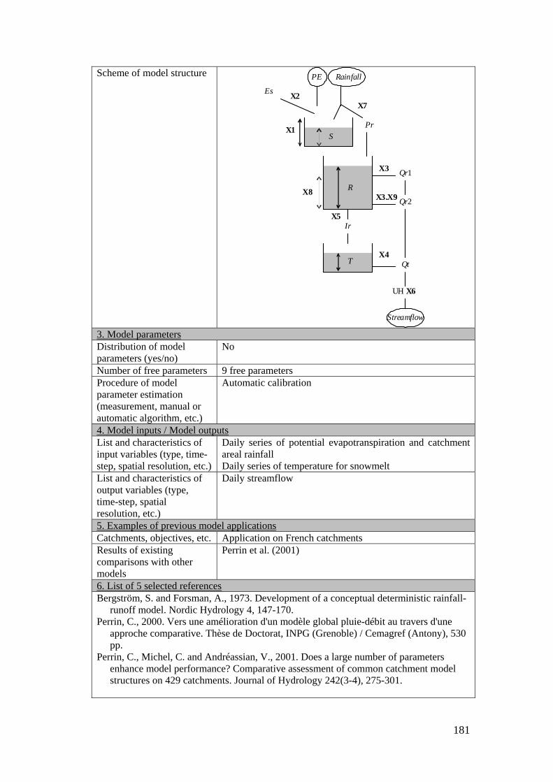
181
Scheme of model structure
Es
Rainfall
UH X6
Streamflow
Qr1
Qr2
S
R
X5
X7
PE
X8
Ir
Pr
T Qt
X1
X2
X4
X3
X3.X9
3. Model parameters Distribution of model parameters (yes/no)
No
Number of free parameters 9 free parameters Procedure of model parameter estimation (measurement, manual or automatic algorithm, etc.)
Automatic calibration
4. Model inputs / Model outputs List and characteristics of input variables (type, time-step, spatial resolution, etc.)
Daily series of potential evapotranspiration and catchment areal rainfall Daily series of temperature for snowmelt
List and characteristics of output variables (type, time-step, spatial resolution, etc.)
Daily streamflow
5. Examples of previous model applications Catchments, objectives, etc. Application on French catchments Results of existing comparisons with other models
Perrin et al. (2001)
6. List of 5 selected references Bergström, S. and Forsman, A., 1973. Development of a conceptual deterministic rainfall-
runoff model. Nordic Hydrology 4, 147-170. Perrin, C., 2000. Vers une amélioration d'un modèle global pluie-débit au travers d'une
approche comparative. Thèse de Doctorat, INPG (Grenoble) / Cemagref (Antony), 530 pp.
Perrin, C., Michel, C. and Andréassian, V., 2001. Does a large number of parameters enhance model performance? Comparative assessment of common catchment model structures on 429 catchments. Journal of Hydrology 242(3-4), 275-301.
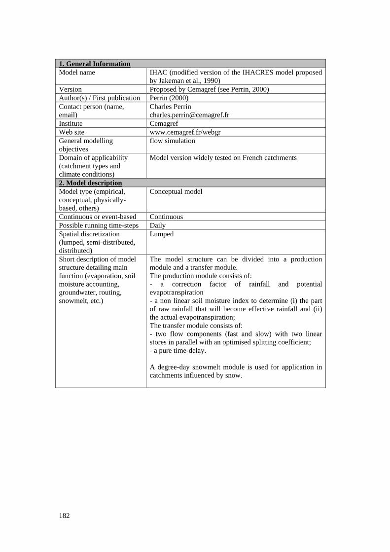
182
1. General Information Model name IHAC (modified version of the IHACRES model proposed
by Jakeman et al., 1990) Version Proposed by Cemagref (see Perrin, 2000) Author(s) / First publication Perrin (2000) Contact person (name, email)
Charles Perrin [email protected]
Institute Cemagref Web site www.cemagref.fr/webgr General modelling objectives
flow simulation
Domain of applicability (catchment types and climate conditions)
Model version widely tested on French catchments
2. Model description Model type (empirical, conceptual, physically-based, others)
Conceptual model
Continuous or event-based Continuous Possible running time-steps Daily Spatial discretization (lumped, semi-distributed, distributed)
Lumped
Short description of model structure detailing main function (evaporation, soil moisture accounting, groundwater, routing, snowmelt, etc.)
The model structure can be divided into a production module and a transfer module. The production module consists of: - a correction factor of rainfall and potential evapotranspiration - a non linear soil moisture index to determine (i) the part of raw rainfall that will become effective rainfall and (ii) the actual evapotranspiration; The transfer module consists of: - two flow components (fast and slow) with two linear stores in parallel with an optimised splitting coefficient; - a pure time-delay. A degree-day snowmelt module is used for application in catchments influenced by snow.
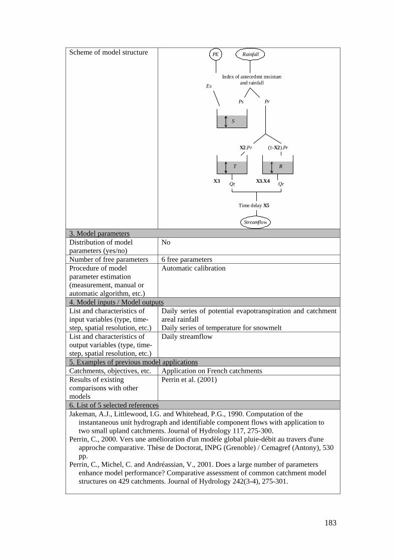
183
Scheme of model structure
Es
Rainfall
Index of antecedent moisture and rainfall
Time delay X5
Pr Ps
X2.Pr (1-X2).Pr
Streamflow
Qr Qt
S
T R
X3 X3.X4
PE
3. Model parameters Distribution of model parameters (yes/no)
No
Number of free parameters 6 free parameters Procedure of model parameter estimation (measurement, manual or automatic algorithm, etc.)
Automatic calibration
4. Model inputs / Model outputs List and characteristics of input variables (type, time-step, spatial resolution, etc.)
Daily series of potential evapotranspiration and catchment areal rainfall Daily series of temperature for snowmelt
List and characteristics of output variables (type, time-step, spatial resolution, etc.)
Daily streamflow
5. Examples of previous model applications Catchments, objectives, etc. Application on French catchments Results of existing comparisons with other models
Perrin et al. (2001)
6. List of 5 selected references Jakeman, A.J., Littlewood, I.G. and Whitehead, P.G., 1990. Computation of the
instantaneous unit hydrograph and identifiable component flows with application to two small upland catchments. Journal of Hydrology 117, 275-300.
Perrin, C., 2000. Vers une amélioration d'un modèle global pluie-débit au travers d'une approche comparative. Thèse de Doctorat, INPG (Grenoble) / Cemagref (Antony), 530 pp.
Perrin, C., Michel, C. and Andréassian, V., 2001. Does a large number of parameters enhance model performance? Comparative assessment of common catchment model structures on 429 catchments. Journal of Hydrology 242(3-4), 275-301.
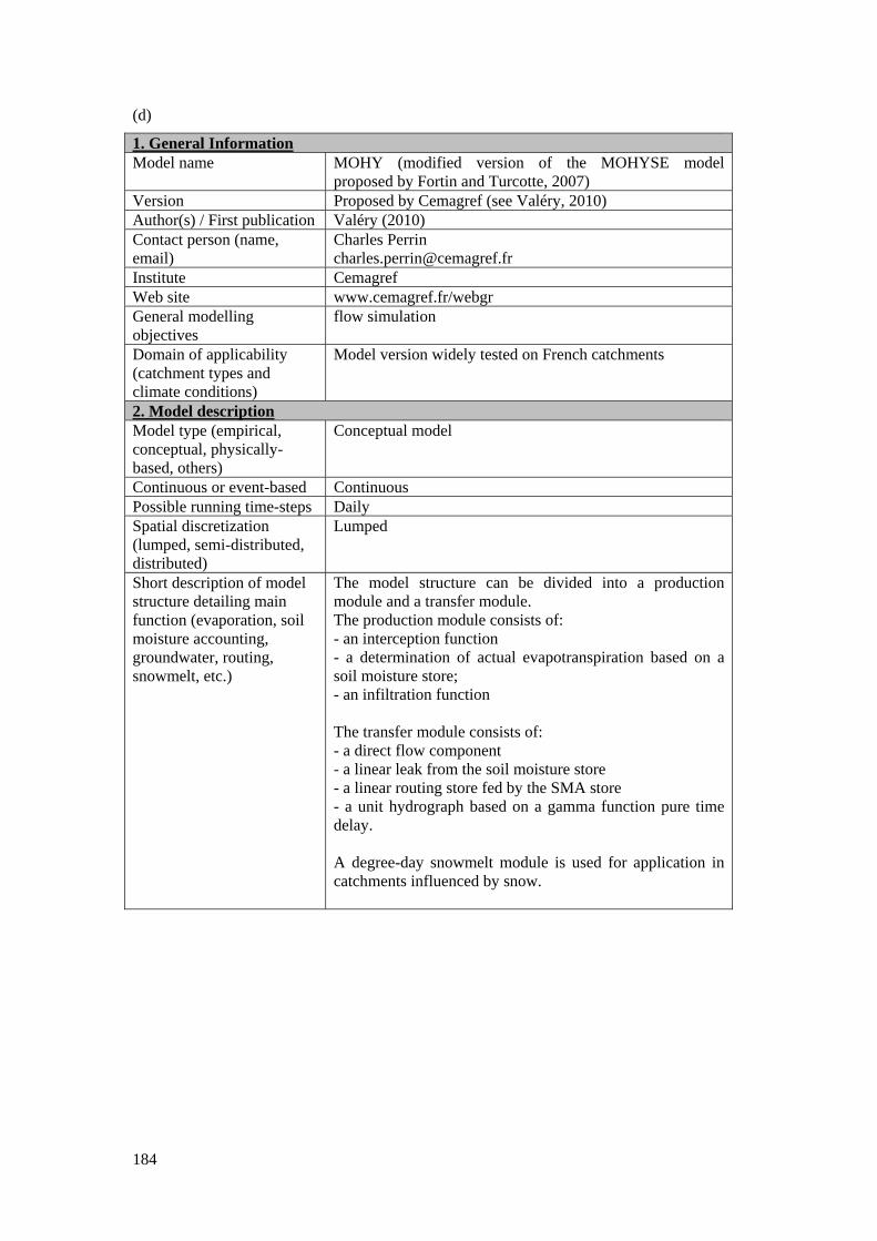
184
(d)
1. General Information Model name MOHY (modified version of the MOHYSE model
proposed by Fortin and Turcotte, 2007) Version Proposed by Cemagref (see Valéry, 2010) Author(s) / First publication Valéry (2010) Contact person (name, email)
Charles Perrin [email protected]
Institute Cemagref Web site www.cemagref.fr/webgr General modelling objectives
flow simulation
Domain of applicability (catchment types and climate conditions)
Model version widely tested on French catchments
2. Model description Model type (empirical, conceptual, physically-based, others)
Conceptual model
Continuous or event-based Continuous Possible running time-steps Daily Spatial discretization (lumped, semi-distributed, distributed)
Lumped
Short description of model structure detailing main function (evaporation, soil moisture accounting, groundwater, routing, snowmelt, etc.)
The model structure can be divided into a production module and a transfer module. The production module consists of: - an interception function - a determination of actual evapotranspiration based on a soil moisture store; - an infiltration function The transfer module consists of: - a direct flow component - a linear leak from the soil moisture store - a linear routing store fed by the SMA store - a unit hydrograph based on a gamma function pure time delay. A degree-day snowmelt module is used for application in catchments influenced by snow.
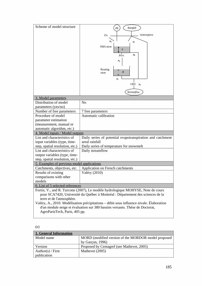
185
Scheme of model structure
PE Rainfall
interception
UH2
Streamflow
x1
S
R
Perc
SMA store
Routing store
x4
x6
En
x2
x5
x7
3. Model parameters Distribution of model parameters (yes/no)
No
Number of free parameters 7 free parameters Procedure of model parameter estimation (measurement, manual or automatic algorithm, etc.)
Automatic calibration
4. Model inputs / Model outputs List and characteristics of input variables (type, time-step, spatial resolution, etc.)
Daily series of potential evapotranspiration and catchment areal rainfall Daily series of temperature for snowmelt
List and characteristics of output variables (type, time-step, spatial resolution, etc.)
Daily streamflow
5. Examples of previous model applications Catchments, objectives, etc. Application on French catchments Results of existing comparisons with other models
Valéry (2010)
6. List of 5 selected references Fortin, V., and R. Turcotte (2007), Le modèle hydrologique MOHYSE, Note de cours
pour SCA7420, Université du Québec à Montréal : Département des sciences de la terre et de l'atmosphère.
Valéry, A., 2010. Modélisation précipitations – débit sous influence nivale. Élaboration d'un module neige et évaluation sur 380 bassins versants. Thèse de Doctorat, AgroParisTech, Paris, 405 pp.
(e)
1. General Information Model name MORD (modified version of the MORDOR model proposed
by Garçon, 1996) Version Proposed by Cemagref (see Mathevet, 2005) Author(s) / First publication
Mathevet (2005)
186
Contact person (name, email)
Charles Perrin [email protected]
Institute Cemagref Web site www.cemagref.fr/webgr General modelling objectives
flow simulation
Domain of applicability (catchment types and climate conditions)
Model version widely tested on French catchments
2. Model description Model type (empirical, conceptual, physically-based, others)
Conceptual model
Continuous or event-based Continuous Possible running time-steps Daily Spatial discretization (lumped, semi-distributed, distributed)
Lumped
Short description of model structure detailing main function (evaporation, soil moisture accounting, groundwater, routing, snowmelt, etc.)
The model structure can be divided into a production module and a transfer module. The production module consists of: - a correction factor of rainfall - a non linear soil moisture index to determine (i) the part of raw rainfall that will become effective rainfall and (ii) the actual evapotranspiration; - a lower store in which remaining PE acts The transfer module consists of: - a direct flow component - an infiltration store - a linear routing store - a unit hydrograph. A degree-day snowmelt module is used for application in catchments influenced by snow.
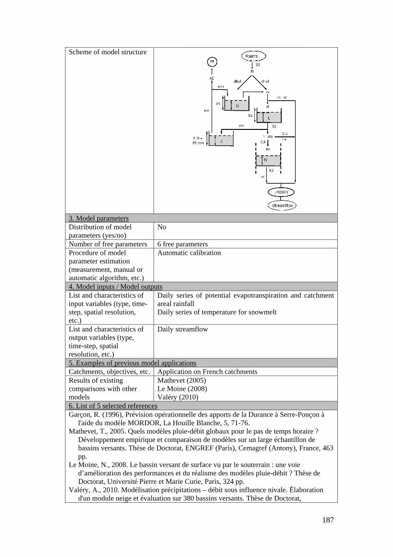
187
Scheme of model structure
3. Model parameters Distribution of model parameters (yes/no)
No
Number of free parameters 6 free parameters Procedure of model parameter estimation (measurement, manual or automatic algorithm, etc.)
Automatic calibration
4. Model inputs / Model outputs List and characteristics of input variables (type, time-step, spatial resolution, etc.)
Daily series of potential evapotranspiration and catchment areal rainfall Daily series of temperature for snowmelt
List and characteristics of output variables (type, time-step, spatial resolution, etc.)
Daily streamflow
5. Examples of previous model applications Catchments, objectives, etc. Application on French catchments Results of existing comparisons with other models
Mathevet (2005) Le Moine (2008) Valéry (2010)
6. List of 5 selected references Garçon, R. (1996), Prévision opérationnelle des apports de la Durance à Serre-Ponçon à
l'aide du modèle MORDOR, La Houille Blanche, 5, 71-76. Mathevet, T., 2005. Quels modèles pluie-débit globaux pour le pas de temps horaire ?
Développement empirique et comparaison de modèles sur un large échantillon de bassins versants. Thèse de Doctorat, ENGREF (Paris), Cemagref (Antony), France, 463 pp.
Le Moine, N., 2008. Le bassin versant de surface vu par le souterrain : une voie d’amélioration des performances et du réalisme des modèles pluie-débit ? Thèse de Doctorat, Université Pierre et Marie Curie, Paris, 324 pp.
Valéry, A., 2010. Modélisation précipitations – débit sous influence nivale. Élaboration d'un module neige et évaluation sur 380 bassins versants. Thèse de Doctorat,
188
AgroParisTech, Paris, 405 pp.
(f)
1. General Information Model name TOPM (modified version of the TOPMODEL model
proposed by Beven and Kirkby, 1996) Version Proposed by Cemagref (see Michel et al., 2003) Author(s) / First publication Michel et al. (2003) Contact person (name, email)
Charles Perrin [email protected]
Institute Cemagref Web site www.cemagref.fr/webgr General modelling objectives
flow simulation
Domain of applicability (catchment types and climate conditions)
Model version widely tested on French catchments
2. Model description Model type (empirical, conceptual, physically-based, others)
Conceptual model
Continuous or event-based Continuous Possible running time-steps Daily Spatial discretization (lumped, semi-distributed, distributed)
Lumped
Short description of model structure detailing main function (evaporation, soil moisture accounting, groundwater, routing, snowmelt, etc.)
The model structure can be divided into a production module and a transfer module. The production module consists of: - an interception store - a non linear soil moisture store used to split net rainfall into two components through a logistic function representing the distribution of the topographic index in the orifinal model - a function to determine the actual evapotranspiration from the soil moisture store; - The transfer module consists of: - two flow components, one routed through a quadratic store, the other routed by an exponential store - a pure time-delay. A degree-day snowmelt module is used for application in catchments influenced by snow.
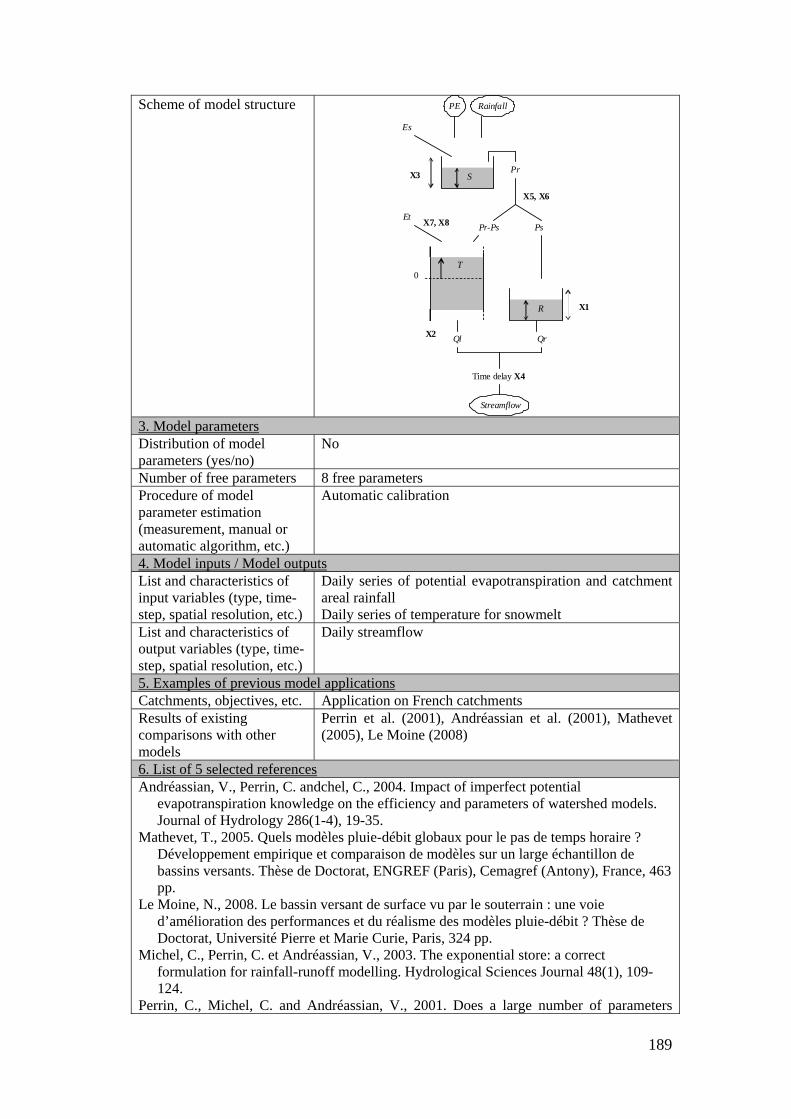
189
Scheme of model structure
Es
Rainfall
Time delay X4
Pr
PsPr-Ps
Streamflow
Qr Ql
S
R
X2
X1
PE
Et
X3
0T
X7, X8
X5, X6
3. Model parameters Distribution of model parameters (yes/no)
No
Number of free parameters 8 free parameters Procedure of model parameter estimation (measurement, manual or automatic algorithm, etc.)
Automatic calibration
4. Model inputs / Model outputs List and characteristics of input variables (type, time-step, spatial resolution, etc.)
Daily series of potential evapotranspiration and catchment areal rainfall Daily series of temperature for snowmelt
List and characteristics of output variables (type, time-step, spatial resolution, etc.)
Daily streamflow
5. Examples of previous model applications Catchments, objectives, etc. Application on French catchments Results of existing comparisons with other models
Perrin et al. (2001), Andréassian et al. (2001), Mathevet (2005), Le Moine (2008)
6. List of 5 selected references Andréassian, V., Perrin, C. andchel, C., 2004. Impact of imperfect potential
evapotranspiration knowledge on the efficiency and parameters of watershed models. Journal of Hydrology 286(1-4), 19-35.
Mathevet, T., 2005. Quels modèles pluie-débit globaux pour le pas de temps horaire ? Développement empirique et comparaison de modèles sur un large échantillon de bassins versants. Thèse de Doctorat, ENGREF (Paris), Cemagref (Antony), France, 463 pp.
Le Moine, N., 2008. Le bassin versant de surface vu par le souterrain : une voie d’amélioration des performances et du réalisme des modèles pluie-débit ? Thèse de Doctorat, Université Pierre et Marie Curie, Paris, 324 pp.
Michel, C., Perrin, C. et Andréassian, V., 2003. The exponential store: a correct formulation for rainfall-runoff modelling. Hydrological Sciences Journal 48(1), 109-124.
Perrin, C., Michel, C. and Andréassian, V., 2001. Does a large number of parameters

190
enhance model performance? Comparative assessment of common catchment model structures on 429 catchments. Journal of Hydrology 242(3-4), 275-301.
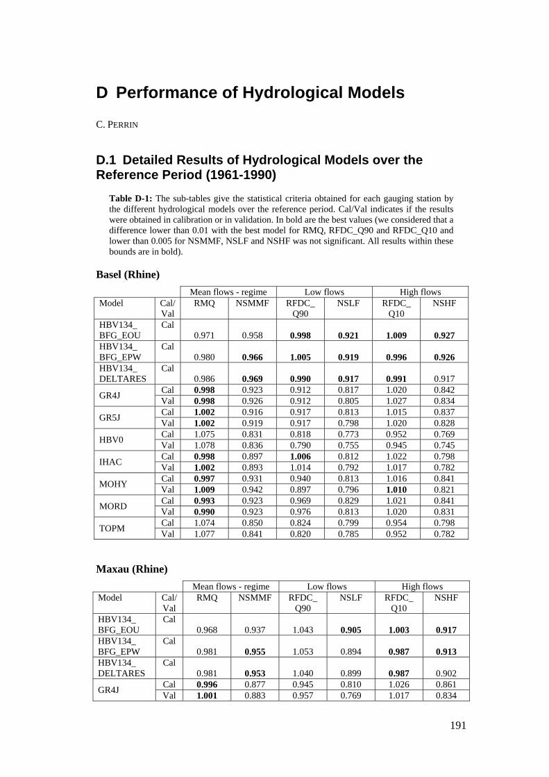
191
D Performance of Hydrological Models
C. PERRIN
D.1 Detailed Results of Hydrological Models over the Reference Period (1961-1990)
Table D-1: The sub-tables give the statistical criteria obtained for each gauging station by the different hydrological models over the reference period. Cal/Val indicates if the results were obtained in calibration or in validation. In bold are the best values (we considered that a difference lower than 0.01 with the best model for RMQ, RFDC_Q90 and RFDC_Q10 and lower than 0.005 for NSMMF, NSLF and NSHF was not significant. All results within these bounds are in bold).
Basel (Rhine) Mean flows - regime Low flows High flows Model Cal/
Val RMQ NSMMF RFDC_
Q90 NSLF RFDC_
Q10 NSHF
HBV134_ BFG_EOU
Cal 0.971 0.958 0.998 0.921 1.009 0.927
HBV134_ BFG_EPW
Cal 0.980 0.966 1.005 0.919 0.996 0.926
HBV134_ DELTARES
Cal 0.986 0.969 0.990 0.917 0.991 0.917
GR4J Cal 0.998 0.923 0.912 0.817 1.020 0.842 Val 0.998 0.926 0.912 0.805 1.027 0.834
GR5J Cal 1.002 0.916 0.917 0.813 1.015 0.837 Val 1.002 0.919 0.917 0.798 1.020 0.828
HBV0 Cal 1.075 0.831 0.818 0.773 0.952 0.769 Val 1.078 0.836 0.790 0.755 0.945 0.745
IHAC Cal 0.998 0.897 1.006 0.812 1.022 0.798 Val 1.002 0.893 1.014 0.792 1.017 0.782
MOHY Cal 0.997 0.931 0.940 0.813 1.016 0.841 Val 1.009 0.942 0.897 0.796 1.010 0.821
MORD Cal 0.993 0.923 0.969 0.829 1.021 0.841 Val 0.990 0.923 0.976 0.813 1.020 0.831
TOPM Cal 1.074 0.850 0.824 0.799 0.954 0.798 Val 1.077 0.841 0.820 0.785 0.952 0.782
Maxau (Rhine) Mean flows - regime Low flows High flows Model Cal/
Val RMQ NSMMF RFDC_
Q90 NSLF RFDC_
Q10 NSHF
HBV134_ BFG_EOU
Cal 0.968 0.937 1.043 0.905 1.003 0.917
HBV134_ BFG_EPW
Cal 0.981 0.955 1.053 0.894 0.987 0.913
HBV134_ DELTARES
Cal 0.981 0.953 1.040 0.899 0.987 0.902
GR4J Cal 0.996 0.877 0.945 0.810 1.026 0.861 Val 1.001 0.883 0.957 0.769 1.017 0.834
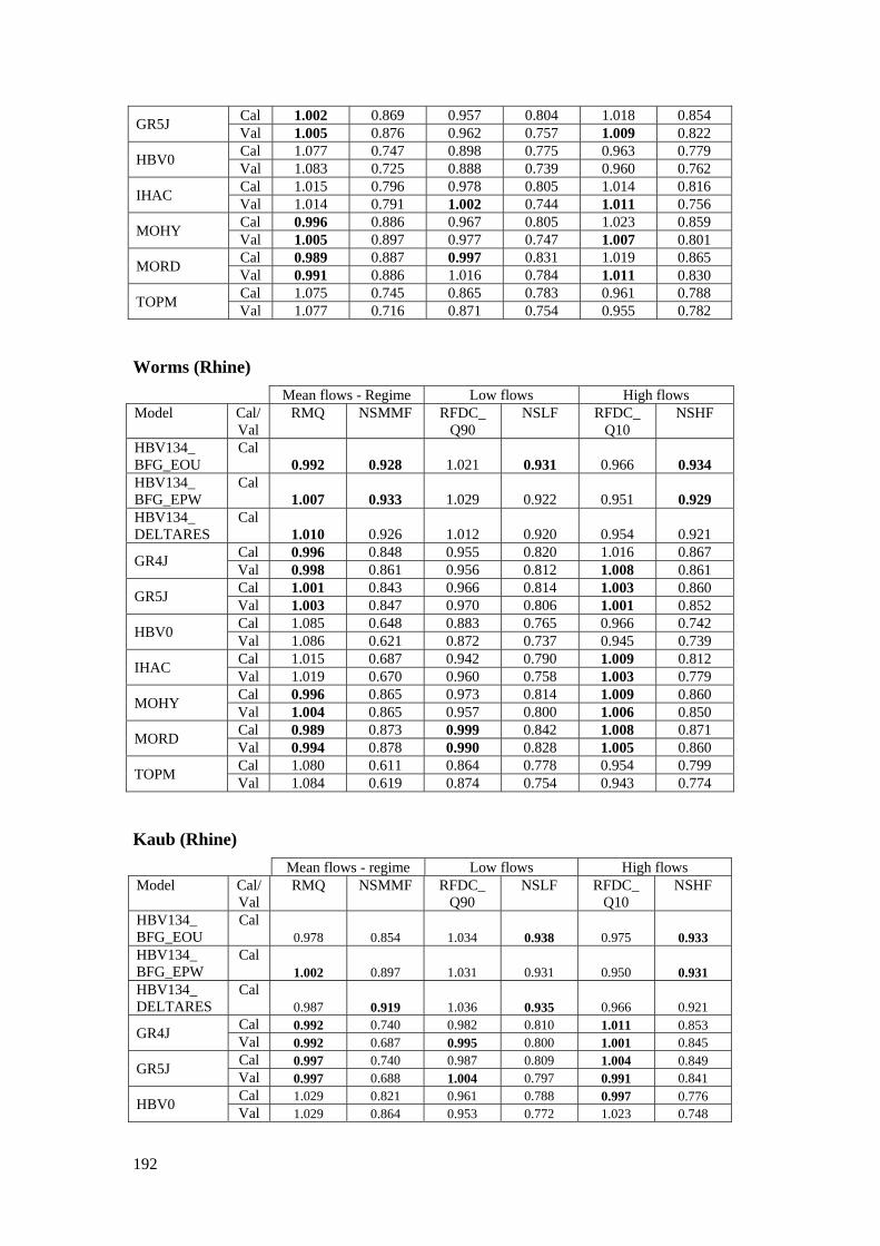
192
GR5J Cal 1.002 0.869 0.957 0.804 1.018 0.854 Val 1.005 0.876 0.962 0.757 1.009 0.822
HBV0 Cal 1.077 0.747 0.898 0.775 0.963 0.779 Val 1.083 0.725 0.888 0.739 0.960 0.762
IHAC Cal 1.015 0.796 0.978 0.805 1.014 0.816 Val 1.014 0.791 1.002 0.744 1.011 0.756
MOHY Cal 0.996 0.886 0.967 0.805 1.023 0.859 Val 1.005 0.897 0.977 0.747 1.007 0.801
MORD Cal 0.989 0.887 0.997 0.831 1.019 0.865 Val 0.991 0.886 1.016 0.784 1.011 0.830
TOPM Cal 1.075 0.745 0.865 0.783 0.961 0.788 Val 1.077 0.716 0.871 0.754 0.955 0.782
Worms (Rhine) Mean flows - Regime Low flows High flows Model Cal/
Val RMQ NSMMF RFDC_
Q90 NSLF RFDC_
Q10 NSHF
HBV134_ BFG_EOU
Cal 0.992 0.928 1.021 0.931 0.966 0.934
HBV134_ BFG_EPW
Cal 1.007 0.933 1.029 0.922 0.951 0.929
HBV134_ DELTARES
Cal 1.010 0.926 1.012 0.920 0.954 0.921
GR4J Cal 0.996 0.848 0.955 0.820 1.016 0.867 Val 0.998 0.861 0.956 0.812 1.008 0.861
GR5J Cal 1.001 0.843 0.966 0.814 1.003 0.860 Val 1.003 0.847 0.970 0.806 1.001 0.852
HBV0 Cal 1.085 0.648 0.883 0.765 0.966 0.742 Val 1.086 0.621 0.872 0.737 0.945 0.739
IHAC Cal 1.015 0.687 0.942 0.790 1.009 0.812 Val 1.019 0.670 0.960 0.758 1.003 0.779
MOHY Cal 0.996 0.865 0.973 0.814 1.009 0.860 Val 1.004 0.865 0.957 0.800 1.006 0.850
MORD Cal 0.989 0.873 0.999 0.842 1.008 0.871 Val 0.994 0.878 0.990 0.828 1.005 0.860
TOPM Cal 1.080 0.611 0.864 0.778 0.954 0.799 Val 1.084 0.619 0.874 0.754 0.943 0.774
Kaub (Rhine) Mean flows - regime Low flows High flows Model Cal/
Val RMQ NSMMF RFDC_
Q90 NSLF RFDC_
Q10 NSHF
HBV134_ BFG_EOU
Cal 0.978 0.854 1.034 0.938 0.975 0.933
HBV134_ BFG_EPW
Cal 1.002 0.897 1.031 0.931 0.950 0.931
HBV134_ DELTARES
Cal 0.987 0.919 1.036 0.935 0.966 0.921
GR4J Cal 0.992 0.740 0.982 0.810 1.011 0.853 Val 0.992 0.687 0.995 0.800 1.001 0.845
GR5J Cal 0.997 0.740 0.987 0.809 1.004 0.849 Val 0.997 0.688 1.004 0.797 0.991 0.841
HBV0 Cal 1.029 0.821 0.961 0.788 0.997 0.776 Val 1.029 0.864 0.953 0.772 1.023 0.748
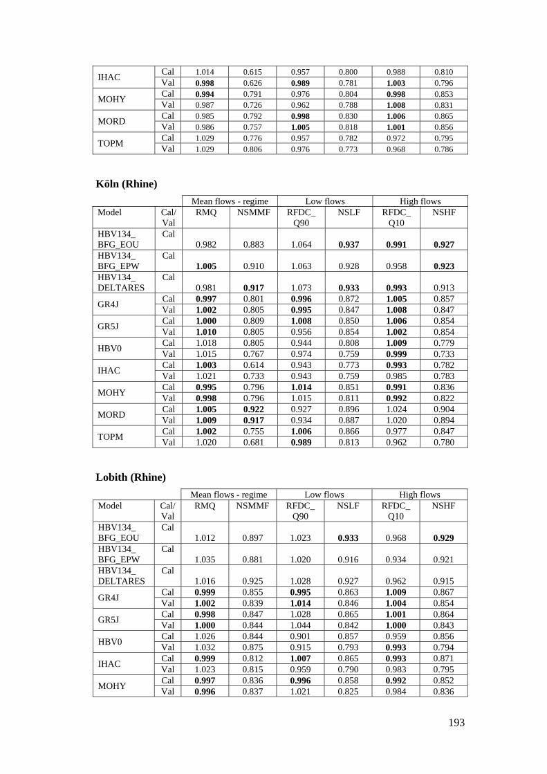
193
IHAC Cal 1.014 0.615 0.957 0.800 0.988 0.810 Val 0.998 0.626 0.989 0.781 1.003 0.796
MOHY Cal 0.994 0.791 0.976 0.804 0.998 0.853 Val 0.987 0.726 0.962 0.788 1.008 0.831
MORD Cal 0.985 0.792 0.998 0.830 1.006 0.865 Val 0.986 0.757 1.005 0.818 1.001 0.856
TOPM Cal 1.029 0.776 0.957 0.782 0.972 0.795 Val 1.029 0.806 0.976 0.773 0.968 0.786
Köln (Rhine) Mean flows - regime Low flows High flows Model Cal/
Val RMQ NSMMF RFDC_
Q90 NSLF RFDC_
Q10 NSHF
HBV134_ BFG_EOU
Cal 0.982 0.883 1.064 0.937 0.991 0.927
HBV134_ BFG_EPW
Cal 1.005 0.910 1.063 0.928 0.958 0.923
HBV134_ DELTARES
Cal 0.981 0.917 1.073 0.933 0.993 0.913
GR4J Cal 0.997 0.801 0.996 0.872 1.005 0.857 Val 1.002 0.805 0.995 0.847 1.008 0.847
GR5J Cal 1.000 0.809 1.008 0.850 1.006 0.854 Val 1.010 0.805 0.956 0.854 1.002 0.854
HBV0 Cal 1.018 0.805 0.944 0.808 1.009 0.779 Val 1.015 0.767 0.974 0.759 0.999 0.733
IHAC Cal 1.003 0.614 0.943 0.773 0.993 0.782 Val 1.021 0.733 0.943 0.759 0.985 0.783
MOHY Cal 0.995 0.796 1.014 0.851 0.991 0.836 Val 0.998 0.796 1.015 0.811 0.992 0.822
MORD Cal 1.005 0.922 0.927 0.896 1.024 0.904 Val 1.009 0.917 0.934 0.887 1.020 0.894
TOPM Cal 1.002 0.755 1.006 0.866 0.977 0.847 Val 1.020 0.681 0.989 0.813 0.962 0.780
Lobith (Rhine) Mean flows - regime Low flows High flows Model Cal/
Val RMQ NSMMF RFDC_
Q90 NSLF RFDC_
Q10 NSHF
HBV134_ BFG_EOU
Cal 1.012 0.897 1.023 0.933 0.968 0.929
HBV134_ BFG_EPW
Cal 1.035 0.881 1.020 0.916 0.934 0.921
HBV134_ DELTARES
Cal 1.016 0.925 1.028 0.927 0.962 0.915
GR4J Cal 0.999 0.855 0.995 0.863 1.009 0.867 Val 1.002 0.839 1.014 0.846 1.004 0.854
GR5J Cal 0.998 0.847 1.028 0.865 1.001 0.864 Val 1.000 0.844 1.044 0.842 1.000 0.843
HBV0 Cal 1.026 0.844 0.901 0.857 0.959 0.856 Val 1.032 0.875 0.915 0.793 0.993 0.794
IHAC Cal 0.999 0.812 1.007 0.865 0.993 0.871 Val 1.023 0.815 0.959 0.790 0.983 0.795
MOHY Cal 0.997 0.836 0.996 0.858 0.992 0.852 Val 0.996 0.837 1.021 0.825 0.984 0.836
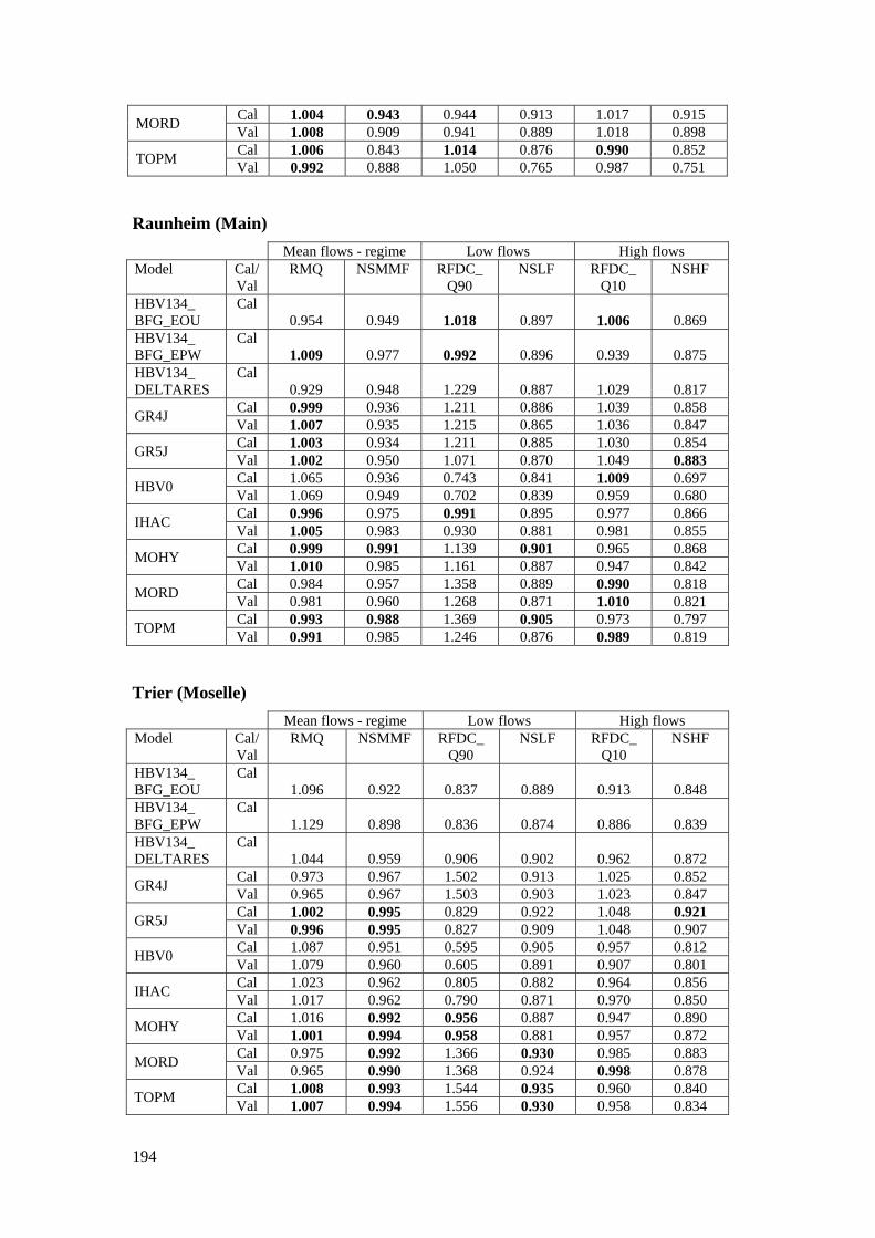
194
MORD Cal 1.004 0.943 0.944 0.913 1.017 0.915 Val 1.008 0.909 0.941 0.889 1.018 0.898
TOPM Cal 1.006 0.843 1.014 0.876 0.990 0.852 Val 0.992 0.888 1.050 0.765 0.987 0.751
Raunheim (Main) Mean flows - regime Low flows High flows Model Cal/
Val RMQ NSMMF RFDC_
Q90 NSLF RFDC_
Q10 NSHF
HBV134_ BFG_EOU
Cal 0.954 0.949 1.018 0.897 1.006 0.869
HBV134_ BFG_EPW
Cal 1.009 0.977 0.992 0.896 0.939 0.875
HBV134_ DELTARES
Cal 0.929 0.948 1.229 0.887 1.029 0.817
GR4J Cal 0.999 0.936 1.211 0.886 1.039 0.858 Val 1.007 0.935 1.215 0.865 1.036 0.847
GR5J Cal 1.003 0.934 1.211 0.885 1.030 0.854 Val 1.002 0.950 1.071 0.870 1.049 0.883
HBV0 Cal 1.065 0.936 0.743 0.841 1.009 0.697 Val 1.069 0.949 0.702 0.839 0.959 0.680
IHAC Cal 0.996 0.975 0.991 0.895 0.977 0.866 Val 1.005 0.983 0.930 0.881 0.981 0.855
MOHY Cal 0.999 0.991 1.139 0.901 0.965 0.868 Val 1.010 0.985 1.161 0.887 0.947 0.842
MORD Cal 0.984 0.957 1.358 0.889 0.990 0.818 Val 0.981 0.960 1.268 0.871 1.010 0.821
TOPM Cal 0.993 0.988 1.369 0.905 0.973 0.797 Val 0.991 0.985 1.246 0.876 0.989 0.819
Trier (Moselle) Mean flows - regime Low flows High flows Model Cal/
Val RMQ NSMMF RFDC_
Q90 NSLF RFDC_
Q10 NSHF
HBV134_ BFG_EOU
Cal 1.096 0.922 0.837 0.889 0.913 0.848
HBV134_ BFG_EPW
Cal 1.129 0.898 0.836 0.874 0.886 0.839
HBV134_ DELTARES
Cal 1.044 0.959 0.906 0.902 0.962 0.872
GR4J Cal 0.973 0.967 1.502 0.913 1.025 0.852 Val 0.965 0.967 1.503 0.903 1.023 0.847
GR5J Cal 1.002 0.995 0.829 0.922 1.048 0.921 Val 0.996 0.995 0.827 0.909 1.048 0.907
HBV0 Cal 1.087 0.951 0.595 0.905 0.957 0.812 Val 1.079 0.960 0.605 0.891 0.907 0.801
IHAC Cal 1.023 0.962 0.805 0.882 0.964 0.856 Val 1.017 0.962 0.790 0.871 0.970 0.850
MOHY Cal 1.016 0.992 0.956 0.887 0.947 0.890 Val 1.001 0.994 0.958 0.881 0.957 0.872
MORD Cal 0.975 0.992 1.366 0.930 0.985 0.883 Val 0.965 0.990 1.368 0.924 0.998 0.878
TOPM Cal 1.008 0.993 1.544 0.935 0.960 0.840 Val 1.007 0.994 1.556 0.930 0.958 0.834
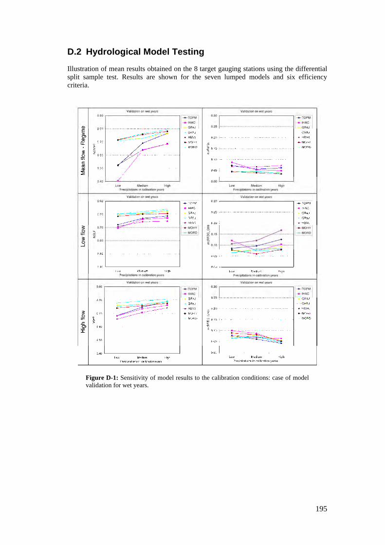
195
D.2 Hydrological Model Testing
Illustration of mean results obtained on the 8 target gauging stations using the differential split sample test. Results are shown for the seven lumped models and six efficiency criteria.
Figure D-1: Sensitivity of model results to the calibration conditions: case of model validation for wet years.
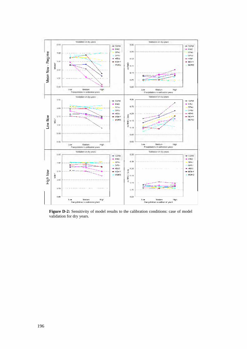
196
Figure D-2: Sensitivity of model results to the calibration conditions: case of model validation for dry years.
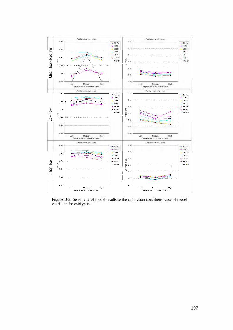
197
Figure D-3: Sensitivity of model results to the calibration conditions: case of model validation for cold years.
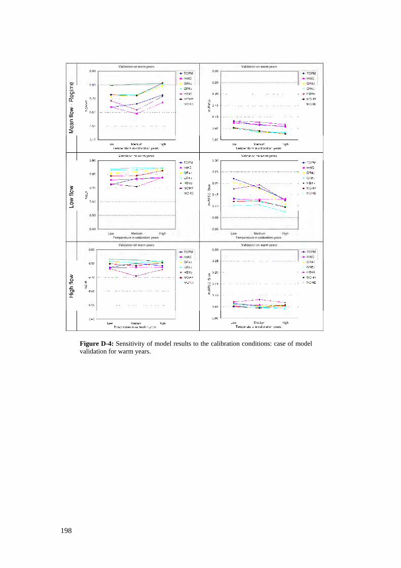
198
Figure D-4: Sensitivity of model results to the calibration conditions: case of model validation for warm years.
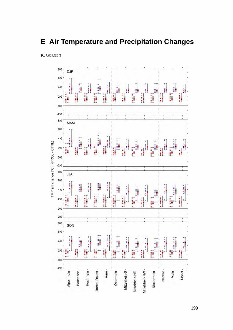
199
E Air Temperature and Precipitation Changes
K. GÖRGEN
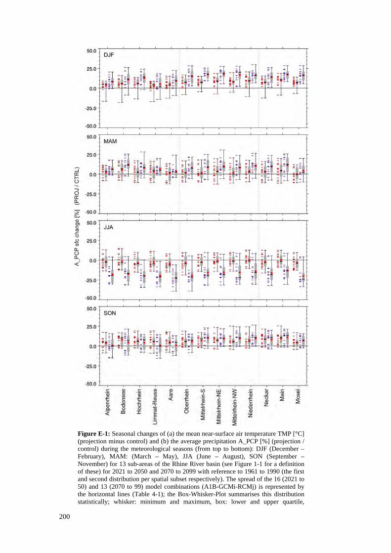
200
Figure E-1: Seasonal changes of (a) the mean near-surface air temperature TMP [°C] (projection minus control) and (b) the average precipitation A_PCP [%] (projection / control) during the meteorological seasons (from top to bottom): DJF (December – February), MAM: (March – May), JJA (June – August), SON (September – November) for 13 sub-areas of the Rhine River basin (see Figure 1-1 for a definition of these) for 2021 to 2050 and 2070 to 2099 with reference to 1961 to 1990 (the first and second distribution per spatial subset respectively). The spread of the 16 (2021 to 50) and 13 (2070 to 99) model combinations (A1B-GCMi-RCMj) is represented by the horizontal lines (Table 4-1); the Box-Whisker-Plot summarises this distribution statistically; whisker: minimum and maximum, box: lower and upper quartile,

201
horizontal line and value: median, red dot: arithmetic mean. Base data: ENSEMBLES RT2B, WDCC; bias-correction: LS (Section 2.2.2). Vertical stippled lines separate Alpine spatial subset, catchments from the analyses subsets immediately along the Rhine and the three major tributaries of Neckar, Main and Mosel on the right hand side of the plot.
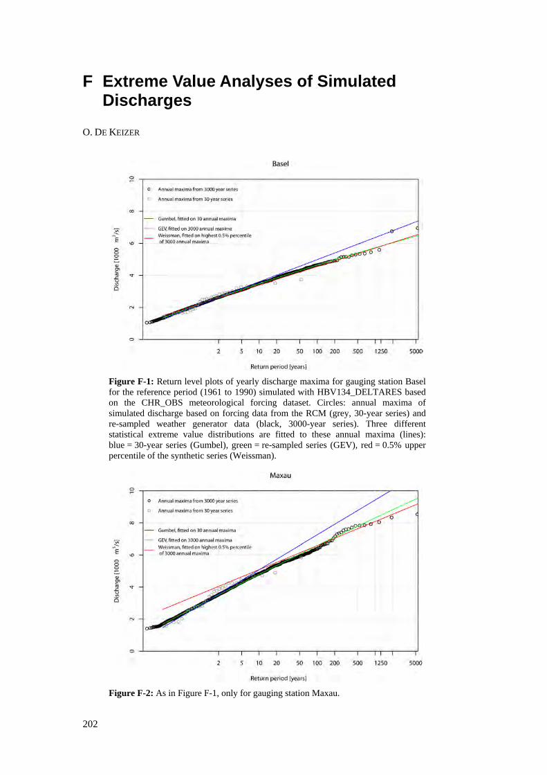
202
F Extreme Value Analyses of Simulated Discharges
O. DE KEIZER
Figure F-1: Return level plots of yearly discharge maxima for gauging station Basel for the reference period (1961 to 1990) simulated with HBV134_DELTARES based on the CHR_OBS meteorological forcing dataset. Circles: annual maxima of simulated discharge based on forcing data from the RCM (grey, 30-year series) and re-sampled weather generator data (black, 3000-year series). Three different statistical extreme value distributions are fitted to these annual maxima (lines): blue = 30-year series (Gumbel), green = re-sampled series (GEV), red = 0.5% upper percentile of the synthetic series (Weissman).
Figure F-2: As in Figure F-1, only for gauging station Maxau.
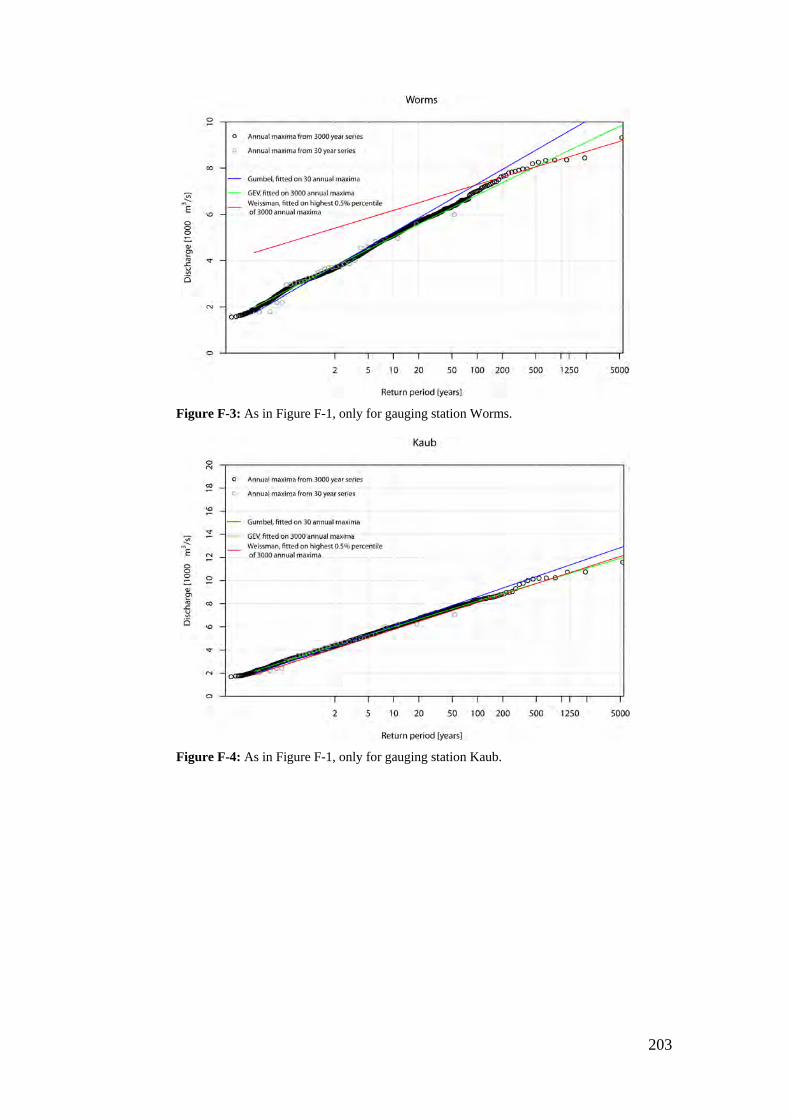
203
Figure F-3: As in Figure F-1, only for gauging station Worms.
Figure F-4: As in Figure F-1, only for gauging station Kaub.
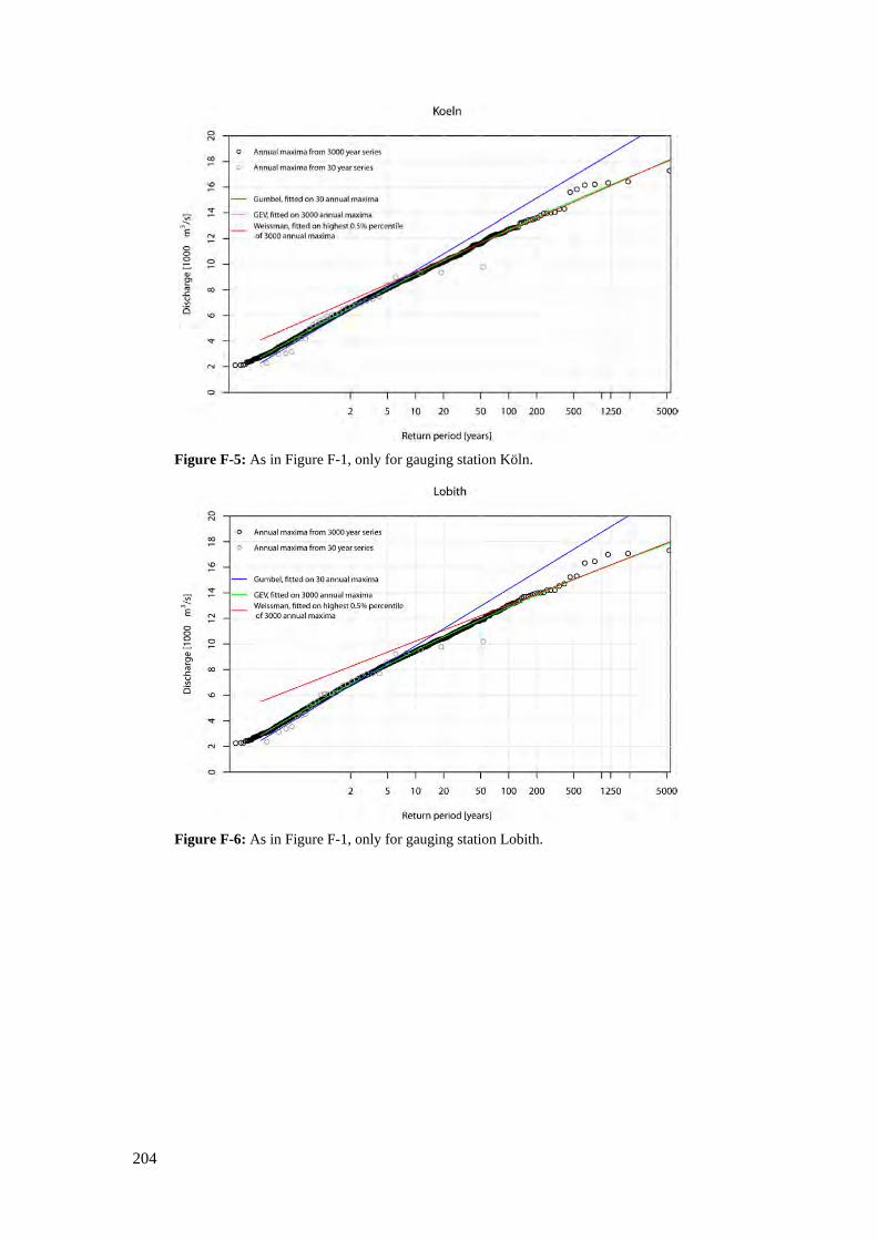
204
Figure F-5: As in Figure F-1, only for gauging station Köln.
Figure F-6: As in Figure F-1, only for gauging station Lobith.
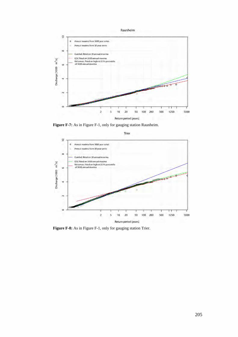
205
Figure F-7: As in Figure F-1, only for gauging station Raunheim.
Figure F-8: As in Figure F-1, only for gauging station Trier.
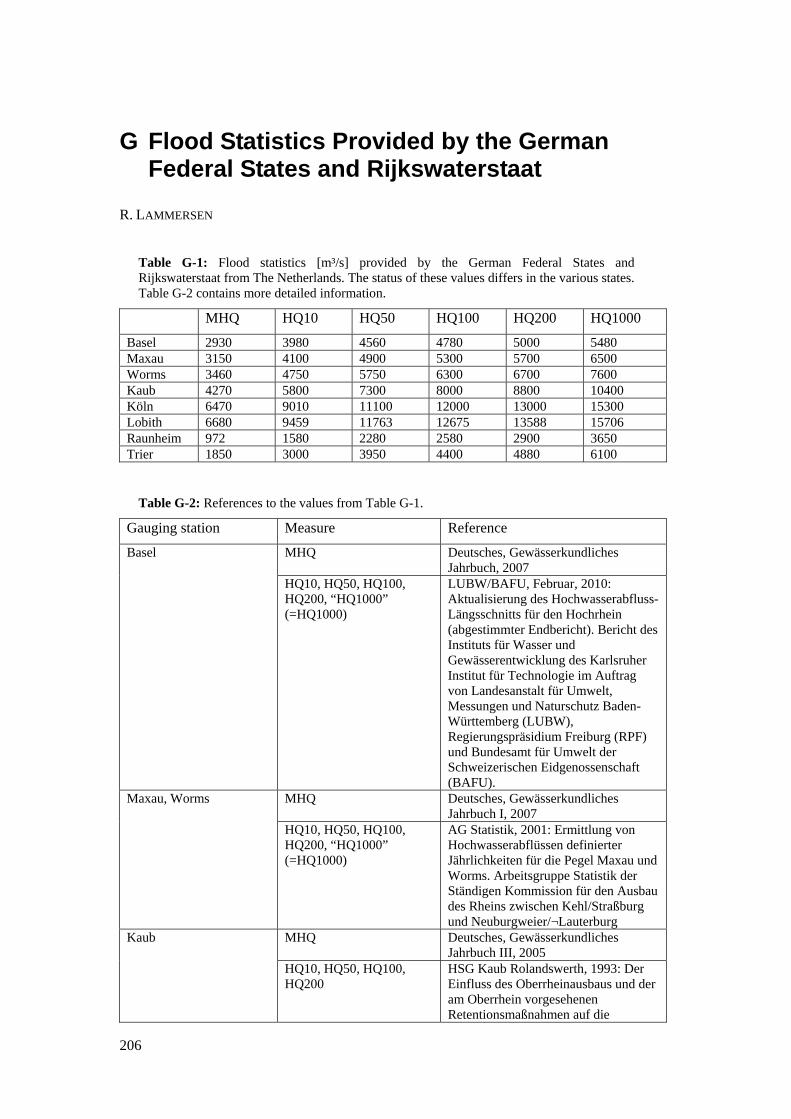
206
G Flood Statistics Provided by the German Federal States and Rijkswaterstaat
R. LAMMERSEN
Table G-1: Flood statistics [m³/s] provided by the German Federal States and Rijkswaterstaat from The Netherlands. The status of these values differs in the various states. Table G-2 contains more detailed information.
MHQ HQ10 HQ50 HQ100 HQ200 HQ1000
Basel 2930 3980 4560 4780 5000 5480 Maxau 3150 4100 4900 5300 5700 6500 Worms 3460 4750 5750 6300 6700 7600 Kaub 4270 5800 7300 8000 8800 10400 Köln 6470 9010 11100 12000 13000 15300 Lobith 6680 9459 11763 12675 13588 15706 Raunheim 972 1580 2280 2580 2900 3650 Trier 1850 3000 3950 4400 4880 6100
Table G-2: References to the values from Table G-1.
Gauging station Measure Reference
Basel MHQ Deutsches, Gewässerkundliches Jahrbuch, 2007
HQ10, HQ50, HQ100, HQ200, “HQ1000” (=HQ1000)
LUBW/BAFU, Februar, 2010: Aktualisierung des Hochwasserabfluss-Längsschnitts für den Hochrhein (abgestimmter Endbericht). Bericht des Instituts für Wasser und Gewässerentwicklung des Karlsruher Institut für Technologie im Auftrag von Landesanstalt für Umwelt, Messungen und Naturschutz Baden-Württemberg (LUBW), Regierungspräsidium Freiburg (RPF) und Bundesamt für Umwelt der Schweizerischen Eidgenossenschaft (BAFU).
Maxau, Worms MHQ Deutsches, Gewässerkundliches Jahrbuch I, 2007
HQ10, HQ50, HQ100, HQ200, “HQ1000” (=HQ1000)
AG Statistik, 2001: Ermittlung von Hochwasserabflüssen definierter Jährlichkeiten für die Pegel Maxau und Worms. Arbeitsgruppe Statistik der Ständigen Kommission für den Ausbau des Rheins zwischen Kehl/Straßburg und Neuburgweier/¬Lauterburg
Kaub MHQ Deutsches, Gewässerkundliches Jahrbuch III, 2005
HQ10, HQ50, HQ100, HQ200
HSG Kaub Rolandswerth, 1993: Der Einfluss des Oberrheinausbaus und der am Oberrhein vorgesehenen Retentionsmaßnahmen auf die
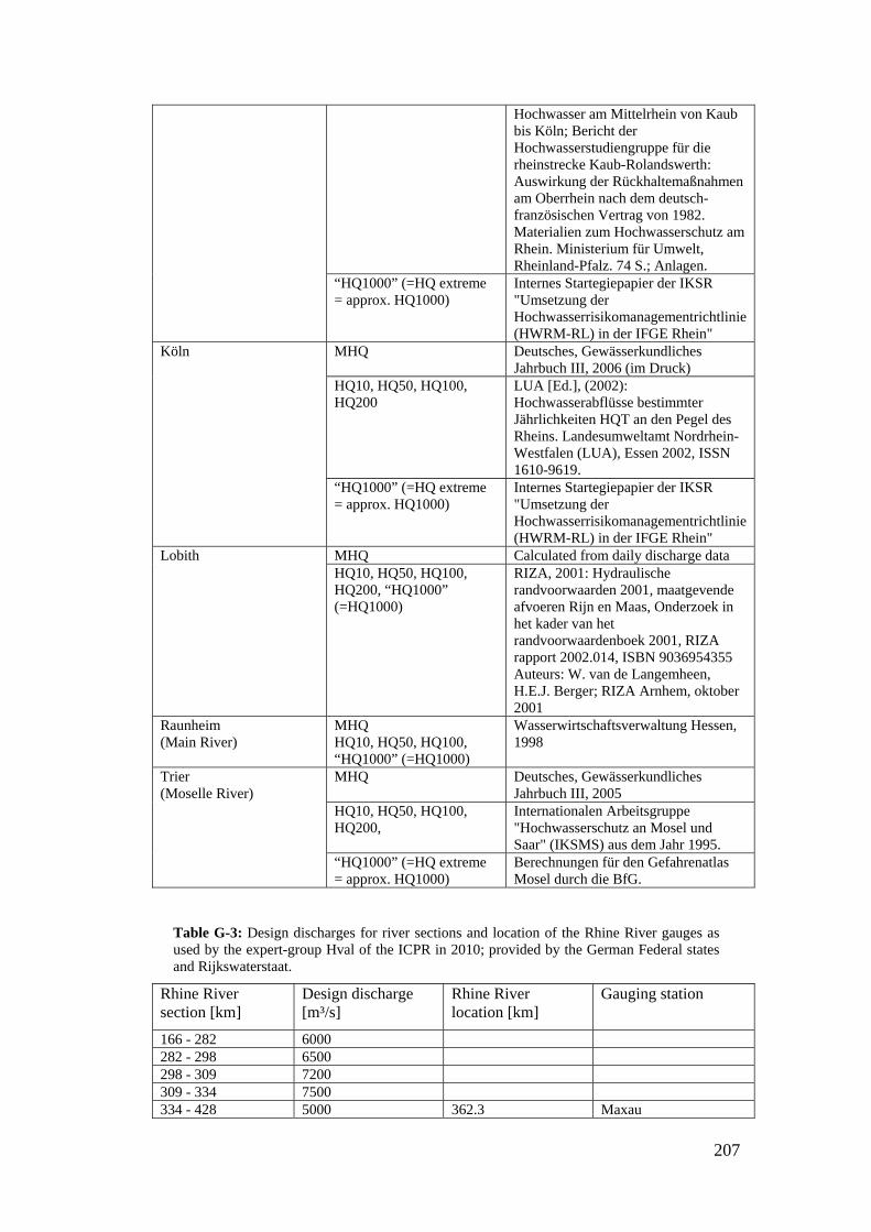
207
Hochwasser am Mittelrhein von Kaub bis Köln; Bericht der Hochwasserstudiengruppe für die rheinstrecke Kaub-Rolandswerth: Auswirkung der Rückhaltemaßnahmen am Oberrhein nach dem deutsch-französischen Vertrag von 1982. Materialien zum Hochwasserschutz am Rhein. Ministerium für Umwelt, Rheinland-Pfalz. 74 S.; Anlagen.
“HQ1000” (=HQ extreme = approx. HQ1000)
Internes Startegiepapier der IKSR "Umsetzung der Hochwasserrisikomanagementrichtlinie (HWRM-RL) in der IFGE Rhein"
Köln MHQ Deutsches, Gewässerkundliches Jahrbuch III, 2006 (im Druck)
HQ10, HQ50, HQ100, HQ200
LUA [Ed.], (2002): Hochwasserabflüsse bestimmter Jährlichkeiten HQT an den Pegel des Rheins. Landesumweltamt Nordrhein-Westfalen (LUA), Essen 2002, ISSN 1610-9619.
“HQ1000” (=HQ extreme = approx. HQ1000)
Internes Startegiepapier der IKSR "Umsetzung der Hochwasserrisikomanagementrichtlinie (HWRM-RL) in der IFGE Rhein"
Lobith MHQ Calculated from daily discharge data HQ10, HQ50, HQ100, HQ200, “HQ1000” (=HQ1000)
RIZA, 2001: Hydraulische randvoorwaarden 2001, maatgevende afvoeren Rijn en Maas, Onderzoek in het kader van het randvoorwaardenboek 2001, RIZA rapport 2002.014, ISBN 9036954355 Auteurs: W. van de Langemheen, H.E.J. Berger; RIZA Arnhem, oktober 2001
Raunheim (Main River)
MHQ HQ10, HQ50, HQ100, “HQ1000” (=HQ1000)
Wasserwirtschaftsverwaltung Hessen, 1998
Trier (Moselle River)
MHQ Deutsches, Gewässerkundliches Jahrbuch III, 2005
HQ10, HQ50, HQ100, HQ200,
Internationalen Arbeitsgruppe "Hochwasserschutz an Mosel und Saar" (IKSMS) aus dem Jahr 1995.
“HQ1000” (=HQ extreme = approx. HQ1000)
Berechnungen für den Gefahrenatlas Mosel durch die BfG.
Table G-3: Design discharges for river sections and location of the Rhine River gauges as used by the expert-group Hval of the ICPR in 2010; provided by the German Federal states and Rijkswaterstaat.
Rhine River section [km]
Design discharge [m³/s]
Rhine River location [km]
Gauging station
166 - 282 6000 282 - 298 6500 298 - 309 7200 309 - 334 7500 334 - 428 5000 362.3 Maxau

208
428 - 497 6000 443.4 Worms 497 - 529 7960 Along the Middle Rhine only local flood defense measures
546.2 Kaub
640 - 659 12600 659 - 780 12900 688.0 Köln 780 - 814 14800 814 - 845 14700 845 - ~ 862 14500 from ~ 862 onwards 16000 862.2 Lobith

209
Additional Material
Additional versioned material like datasets and visualisations may be made available via the CHR website including the respective meta-information and documentation as far as licensing restrictions and/or contributing projects usage-constraints allow it.
http://www.chr-khr.org > Projects > RheinBlick2050 > follow links therein

210
Individual Authors Contributions Overview
Chapter 1 Introduction No specific author assigned
Chapter 2 Overview of Available Data and Processing Procedures
Nilson, Beersma, Perrin, Carambia, Krahe, de Keizer, Görgen
Chapter 3 Evaluation of Data and Processing Procedures
Nilson, Perrin, Beersma, Krahe, Carambia, de Keizer, Görgen
Chapter 4 Meteorological Changes in the Rhine River Basin
Görgen, Nilson
Chapter 5 Changes in Mean Flow in the Rhine River Basin
de Keizer, Carambia, Nilson
Chapter 6 Low Flow Changes in the Rhine River Basin
Nilson, Carambia, Krahe
Chapter 7 High Flow Changes in the Rhine River Basin
de Keizer, Beersma, Lammersen, Buiteveld
Chapter 8 Report Summary and Overall Conclusions
No specific author assigned
Chapter 9 Outlook No specific author assigned
Appendix A Target Measures Görgen
Appendix B Regional Climate Change Projections Data Overview
Nilson
Appendix C Hydrological Model Features Perrin, Carambia, De Keizer
Appendix D Performance of Hydrological Models
Perrin
Appendix E Air Temperature and Precipitation Changes
Görgen
Appendix F Extreme Value Analyses of Simulated Discharges
de Keizer
Appendix G Flood Statistics Provided by the German Federal States and Rijkswaterstaat
Lammersen
211
Colophon
Publication I-23 of the CHR
Secretariat CHR / KHR
PO Box 17
8200 AA Lelystad
The Netherlands
e-mail: [email protected]
web-address: http://www.chr-khr.org
Printer:
Drukkerij Hazenberg BV, Boxtel
ISBN 978-90-70980-35-1
Citation
Chapters can be referenced by their title and authors, if citing the whole report please use:
Görgen, K., Beersma, J., Brahmer, G., Buiteveld, H., Carambia, M., de Keizer, O., Krahe, P., Nilson, E., Lammersen, R., Perrin, C. and Volken, D. (2010) Assessment of Climate Change Impacts on Discharge in the Rhine River Basin: Results of the RheinBlick2050 Project, CHR report, I-23, 229 pp., Lelystad, ISBN 978-90-70980-35-1.
19/09/2010 18:12:00 KG