InstituteforInternationalEconomicPolicyWorkingPaperSeriesElliottSchoolofInternationalAffairsTheGeorgeWashingtonUniversity

InternationalAssetAllocationsandCapitalFlows:TheBenchmarkEffect

IIEP-WP-2017-10

TomasWilliams GeorgeWashingtonUniversity

ClaudioRaddatz

InternationalMonetaryFund

SergioL.SchmuklerWorldBank

August2017InstituteforInternationalEconomicPolicy1957ESt.NW,Suite502Voice:(202)994-5320Fax:(202)994-5477Email:iiep@gwu.eduWeb:www.gwu.edu/~iiep

International Asset Allocations and Capital Flows:

The Benchmark Effect

Claudio Raddatz Sergio L. Schmukler Tomás Williams*

August 2017

Abstract

We study different channels through which well-known benchmark indexes impact asset allocations, capital flows, asset prices, and exchange rates across countries, using unique monthly micro-level data of benchmark compositions and mutual fund investments during 1996-2014. We exploit different events and the presence of countries in multiple benchmarks to study the impact of benchmarks. We find that movements in benchmarks appear to have important effects on equity and bond mutual fund portfolios, including passive and active funds. The effects persist even after controlling for other relevant variables, such as time-varying industry-level factors, country-specific effects, and macroeconomic fundamentals. Exogenous, pre-announced changes in benchmarks impact asset allocations, capital flows, and abnormal returns in asset prices and exchange rates. These systemic effects occur not just when the benchmark changes are announced, but also later on when they become effective. By impacting country allocations, benchmarks explain apparently counterintuitive movements in capital flows and aggregate prices. JEL Classification Codes: F32, F36, G11, G15, G23 Keywords: benchmark indexes, contagion, coordination mechanism, ETFs, international asset prices, international portfolio flows, mutual funds

* This paper is forthcoming in the Journal of International Economics. For financial support, we thank the Hong Kong Institute for Monetary Research and the World Bank Research Department, Knowledge for Change Program, and Latin American and the Caribbean Chief Economist Office. We are grateful to Juan José Cortina, Sebastián Cubela, Julián Kozlowski, Matías Moretti, and Lucas Núñez for excellent research assistance. We received very useful comments from Matías Braun, Fernando Broner (the editor), Guillermo Calvo, Eduardo Cavallo, Nathan Converse, Ganga Darbha, Charles Engel, Eduardo Fernandez Arias, Jose de Gregorio, Gaston Gelos, Bernardo Guimaraes, Marcel Fratzscher, Harald Hau, Lance Kent, Robert Lavigne, Steve Lawrence, Philip Lane, Pedro Matos, Gian Maria Milesi-Ferretti, Guillermo Ordoñez, Ana Pavlova, Luis Serven, Ilhyock Shim, Hyun Song Shin, Carlos Vegh, Frank Warnock, Jialin Yu, Stefan Zeume, two anonymous referees, and participants at presentations held at the Annual Meeting of the Chilean Economic Society, Barcelona GSE Jamboree, Bank of Japan, BIS-Bank of Canada-World Bank Public Investors Conference, CEMP-CIEPS-HKUST IEMS Workshop, Central Bank of Argentina, Columbia University, Cornell University, CREI-Universitat Pompeu Fabra, Fourth Symposium on Emerging Financial Markets: China and Beyond, Global Financial Stability Conference, Honk Kong Institute for Monetary Research, IMF, IADB-Central Banks Conference, Ninth CEPR Annual Workshop on Macroeconomics of Global Interdependence, LACEA Annual Meetings, Latin Finance Network, London Business School, NIPFP, Sao Paulo School of Economics, Universidad Adolfo Ibañez, Universidad de San Andres, University of Virginia Darden School of Business, and World Bank. The views expressed here do not necessarily represent those of the International Monetary Fund or the World Bank. Raddatz is with the International Monetary Fund. Schmukler is with the World Bank Research Department. Williams is with the George Washington University. The views expressed here do not necessarily represent those of the International Monetary Fund or the World Bank. Email addresses: craddatzkiefer@imf.org; sschmukler@worldbank.org; tomaswilliams@gwu.edu.

1

1. Introduction

Several papers argue that benchmark indexes are important for equity prices and how managers

allocate their portfolios across firms.1 In this paper, we show how benchmarks can matter in the

international context, not only for asset allocations but also for capital flows, asset prices, and

exchange rates. In doing so, we depart from the typically studied effects of macroeconomic

fundamentals on cross-country investment decisions, which have been the focus of the

international finance literature.2

The “benchmark effect” refers to various channels through which prominent

international equity and bond market indexes (such as, the MSCI Emerging Markets Index or the

MSCI World Index) affect asset allocations, capital flows, and prices across countries. Theoretical

models predict that the investment strategy of these funds is pinned down by the composition of

their benchmark indexes (Chakravorti and Lall, 2004; Basak and Pavlova, 2012; Deniz and

Pinheiro, 2015). Therefore, changes in the country weights of a popular benchmark can trigger a

similar rebalancing among the funds that track it and result in sizeable movements in financial

markets.3 But the implications of this effect on different variables is not trivial and has not been

systematically documented using cross-country data.

According to the capital asset pricing (CAPM) model, if benchmark indexes perfectly

reflected market weights, their components were atomistic, and their weights were adjusted

instantaneously, investors would hold these indexes and the benchmarks themselves would not

1 Several papers study the importance of benchmarks, focusing primarily on the performance evaluation of mutual funds relative to their benchmarks, in particular, on whether active management pays (Lehmann and Modest, 1987; Sharpe, 1992; Wermers, 2000; Cremers and Petajisto, 2009; Sensoy, 2009; Busse et al., 2014; Cremers et al., 2016). A related literature focuses on how benchmark redefinitions affect stock returns, pricing, and liquidity (Harris and Gurel, 1986; Shleifer, 1986; Chen et al., 2004; Barberis et al., 2005; Greenwood, 2005; Hau et al., 2010; Hau, 2011; Vayanos and Wooley, 2011, 2016; Claessens and Yafeh, 2012; Faias et al., 2012; Bartram at al., 2015; Chang et al., 2015). 2 Some examples of the many papers on the topic are Di Giovanni (2005), Kraay et al. (2005), Lane and Milesi-Ferreti (2007), Antràs and Caballero (2009), Martin and Taddei (2013), Reinhardt et al. (2013), and Gourinchas and Rey (2014). 3 The extent to which fund portfolios are linked to their benchmarks depends on several factors, including the manager’s risk aversion and the correlation among the assets in the benchmark portfolio (Roll, 1992; Brennan, 1993; Disyatat and Gelos, 2001). Moreover, mutual funds declare prospectus benchmarks but they need not follow them (Cremers and Petajisto, 2009). Furthermore, the number of assets in benchmark indexes is much larger than that held in mutual fund portfolios (Didier et al., 2013), which suggests that some funds do not fully replicate these indexes.

2

generate any distortion.4 But benchmark indexes are imperfect and do not necessarily hold the

market portfolio. There are many indexes covering overlapping sets of countries, so their

composition and the decisions of the companies that construct them to include different

countries in different benchmarks can matter for global asset allocations. Moreover, individual

countries tend to have non-negligible weights and can distort different indexes when

included/excluded. As a growing number of international mutual funds and other institutional

investors follow popular benchmarks more passively to cut costs, evaluate and discipline fund

managers, increase transparency, and provide simple investment vehicles (such as, index funds

and exchange-traded funds or ETFs), these effects are expected to increase and need to be

understood and quantified.5

A clear practical example of the benchmark effect took place when Israel was moved

from the MSCI Emerging Markets Index to the World Index (composed of developed markets).

Although the upgrade was announced in advance and occurred because Israel’s fundamentals

had improved (Business Week, 2010), we show that Israel faced significant capital reallocations,

capital outflows, and negative returns when the upgrade became effective due to the behavior of

funds following these indexes. These effects have prompted some to argue for South Korea and

Taiwan not to be upgraded to developed market status (Bloomberg, 2014). Similar discussions

have emerged with the actual and potential upgrades of Portugal (1997), Greece (2001), Qatar

(2014), the United Arab Emirates (U.A.E.) (2014), and China (2015) and the downgrades of

Venezuela (2006), Argentina (2009), and Greece (2013) (Financial Times, 2013a,b,c; BIS, 2014;

The Economist, 2014a). One reason for the effect on capital flows is that a country’s inclusion

(exclusion) in a benchmark index should drive managers with index-tracking strategies to

rebalance their portfolios and direct flows into (out of) that country (The Economist, 2012).

In this paper, we systematically study how benchmarks affect international financial

markets. First, we study to what extent movements in benchmark weights map into movements

in the actual country weights (“weights”) of the funds that declare that benchmark. We exploit

4 Still, price discovery might be hampered, which can exacerbate co-movement across assets (Wurgler, 2011). 5 Other problems can arise due to the use of benchmark weights to overcome agency problems, but these issues are not examined in the empirical analysis of this paper.

3

the timing of changes in benchmarks and the presence of a country in multiple benchmarks, to

shed light on whether the evidence is consistent with a causal link between benchmarks and

portfolio allocations. Second, we show the consequences that the relation between mutual fund

weights and benchmark weights has for mutual fund flows, and quantify the importance of

benchmarks for capital flows. Third, we use upgrades and downgrades of countries to study how

aggregate asset prices and exchange rates respond to benchmark changes. Fourth, we use several

key cases to illustrate how benchmark changes can impact countries in different ways.

To conduct the research, we compile a novel dataset of detailed portfolio allocations

across countries by a large number of international mutual funds that we match with the

allocations of the benchmarks they follow. The dataset covers the period from January 1996 to

September 2014 and contains international mutual funds based in major financial centers around

the world investing in at least two countries (i.e., it excludes country funds). A total of 2,837

equity and 838 bond funds are in the sample. These equity and bond funds collectively had 1,052

and 293 billion U.S. dollars in assets under management in December 2011, respectively.6

Our results show that benchmarks have statistically and economically significant effects

on the allocations and capital flows of mutual funds across countries. Mutual funds follow

benchmarks rather closely. For example, a 1 percent increase in a country’s benchmark weight

results on average in a 0.7 percent increase in the weight of that country for the typical mutual

fund that follows that benchmark. Explicit indexing funds seem to follow benchmarks almost

one-for-one, generating some mechanical effects in allocations and capital flows. Although the

most active funds in our sample are less connected to the benchmarks, they still seem to be

significantly influenced by their behavior, with about 50 percent of their allocations explained by

benchmarks. The effects on mutual fund portfolios appear relevant even after controlling for

time-varying industry allocations and country-specific or macroeconomic factors, usually

mentioned in the finance and international finance literatures. The results do not seem to be just

the consequence of common shocks affecting both mutual fund weights and benchmark weights

6 Mutual funds are offered to investors in different ways, for example, in different currencies and with different costs. These funds have the same portfolios but many times are counted as separate funds. In our data, we just count them once to avoid repeating the portfolios, but we report their aggregated assets.

4

(via returns) or reverse causality (which could occur as mutual funds reallocate their portfolio,

exerting pressure on returns and benchmark weights). Instead, exogenous events that modify

indexes appear to affect not only benchmark but also mutual fund weights.

By influencing the asset allocations of mutual funds, benchmarks seem to have systemic

effects. In particular, benchmarks can explain nearly 40 percent of capital flows from mutual

funds, with this percentage increasing to 70 percent in times of large exogenous changes to

benchmarks. Moreover, large benchmark changes (such as upgrades and downgrades of

countries) are associated with abnormal returns in asset prices and exchange rates around those

events. These abnormal returns behave as predicted by the mutual fund flows; they become

positive (negative) when inflows to (outflows from) a country are expected. Notably, these

effects are present both during the announcement and effective dates of these changes. For

example, the cumulative asset price differential returns are 1.5 percent around the announcement

date and 3.5 percent around the effective date. Our results suggest that, through the reallocations

they trigger, benchmark changes affect prices beyond the information content of

upgrades/downgrades.

The rest of the paper is organized as follows. Section 2 describes the data. Section 3

studies the effect of benchmarks on mutual fund asset allocations. Section 4 analyzes the relation

between asset allocations and capital flows, and the effects of benchmarks on these flows.

Section 5 studies how asset prices and exchange rates react around benchmark changes. Section 6

presents some case studies that further illustrate the effects on capital flows and asset prices.

Section 7 concludes.

2. Data

Our main database consists of: (i) country weights or weights, 𝑤!" , which are the country

portfolio allocations of international mutual funds (those investing in several countries); (ii)

benchmark weights, 𝑤!"! , which are the country allocations in the relevant benchmarks; (iii)

mutual fund-specific information, such as its assets, returns, and relevant benchmarks; (iv)

5

country-specific information, such as stock and bond market index returns.7 The sub-index i

refers to funds, c to countries, and the supra-index B to benchmarks. For the final database, we

clean the raw data and merge data from several sources, some of which had not been previously

used or matched in the literature. This database covers the period from January 1996 to July 2012

and constitutes an unbalanced panel. We use some additional data (described later in the paper)

to study the reactions of capital flows and asset prices, covering newer episodes up to 2014.

Our database contains 2,837 equity funds and 838 bond funds, including global, global

emerging, and regional funds, whose total net assets (TNAs, 𝐴!") have increased significantly

over time.8 Moreover, funds in our combined dataset capture an important part of the assets held

by the industry of international funds. For example, our sample of U.S.-domiciled equity funds

had 442 billion dollars in TNAs, while the Investment Company Institute (ICI) reports that,

during the same period, U.S. (non-domestic) international funds held 1.4 trillion dollars including

the numerous country funds that we exclude due to our interest on country weights. Similar

estimates for Europe from the European Fund Asset Management Association (EFAMA) show

that our sample accounts for approximately 53 percent of the international funds in this region.

Explicit indexing funds (mostly ETFs) represent a fast growing but still relatively small share of

the industry. By also including closet indexing funds, both the level and growth rate of the funds

that closely track benchmark indexes increases significantly.9

Our two main sources for country portfolio allocations of international mutual funds are

EPFR (Emerging Portfolio Fund Research) and Morningstar Direct (MS). Both sources include

dead and live mutual funds. The data from EPFR are at a monthly frequency, and include open-

end equity and bond funds classified according to their geographical investment scope. Global

funds invest anywhere in the world, global emerging funds only in emerging countries, and

7 Benchmark weights𝑤!"! are fund-specific because each fund chooses its benchmark. We thus denote it with sub-indexi. The same applies to other benchmark characteristics such as benchmark returns.8 In 2011, the equity (bond) funds in our sample had 1.2 trillion (303 billion) U.S. dollars in TNAs (Online Appendix Figure 1). Equity funds are domiciled around the entire world but most of the funds are located in Canada, France, Ireland, Luxembourg, the United States (U.S.), and the United Kingdom (U.K.). Most bond funds are domiciled in Denmark, Germany, Ireland, Israel, Italy, Luxembourg, the U.S., and the U.K. 9 The trends exhibited by the share of total assets of ETFs in our sample also appear in data on U.S. mutual funds from the Investment Company Institute (ICI), which does not identify closet indexing funds.

6

regional funds in groups of countries within a specific geographical region.10 The data also

comprise portfolios of ETFs. We use only funds with information for at least one year. For each

fund i and each month t, the data contain information on the share of the fund’s assets invested

in each of 124 countries and cash, as well as its TNAs. We also have information on static

characteristics, for example, the asset class, domicile, whether a fund is an ETF, its strategy

(passive or active), and, crucially, its declared benchmark. We complement these data with

information on the funds’ net asset value (NAV) from Datastream and MS. We match the funds

from these different databases.

We use similar data from MS to complement the EPFR data. That is, we use data on

country weights, TNAs, NAVs, and static fund characteristics for additional international mutual

funds not included in EPFR with at least one year of monthly data.11 This increases importantly

the cross-sectional coverage of our final dataset. MS reports country weights in only 52 countries

and does not contain data on cash allocations.12 The combination of the two databases provides

us with an extensive cross-sectional and time-series coverage of funds (Online Appendix Table 1).

MS contains a large number of funds after 2007 but very few in earlier years, while EPFR has a

more balanced number of funds dating back to 1996.13 In addition, we use stock and bond

market country indexes from J.P. Morgan and MSCI to compute the country returns, 𝑅!" , which

we impute to each fund’s investment in each country (we do not have information on the actual

returns of each fund in each country).14 This information comes from Datastream and MSCI.

10 While global funds theoretically can invest anywhere in the world, a large proportion of them track the MSCI World Index, which only has developed countries as constituents. A minor proportion of these funds track the MSCI All Country World Index, which contains both developed and emerging countries. 11 Although MS includes funds that report quarterly, almost 90 percent of the original MS sample reports allocations on a monthly frequency.12 In our estimations, we only use country allocations and, thus, do not include the residual category of other countries (those not explicitly reported in the EPFR or MS databases) nor cash. 13 In our consolidated database we kept the country coverage of MS (52 countries) and adapted the EPFR database to this format, lumping countries outside these 52 in a residual category called “other equity” (also present in MS). We have also performed robustness tests for the impact of this change for the EPFR database. The results are qualitatively similar. 14 The correlation between the actual fund returns and the computed returns using country returns is 89 percent, which shows that country returns are a good proxy for individual returns. Some of the small unexplained part is due to differences in the country returns and security level returns, but it might also be due to the fact that the data have a small residual category (“other equity/bonds”) that we cannot assign to any particular country given the information available.

7

In addition to our data on fund country weights, we also use data on the country

benchmark weights and returns of several major benchmark indexes (𝑅!"! ). We obtain these data

directly from FTSE, J.P. Morgan, and MSCI through bilateral agreements, and indirectly through

MS for indexes produced by Dow Jones, Euro Stoxx, and S&P. The benchmarks indexes we use

have different scope and are listed in Online Appendix Table 2. For each of the benchmark

indexes in MS and MSCI, we collect data on price returns, gross returns, and net returns. We rely

heavily on the MSCI benchmark indexes because 86 percent of our data on equity mutual funds

declare to follow them.15 Moreover, we gather daily data from Datastream to analyze the impact

of benchmark changes in asset prices and foreign exchange rates.

To match the data on international mutual funds with the benchmark indexes, we assign

to each fund the index declared in its prospectus. For funds with no declared index, we impute

the benchmark assigned to it by industry analysts, as reported by MS, although the results

reported below are similar when considering only funds that explicitly declare a benchmark. We

were able to match 88 percent of the equity funds and 18 percent of the bond funds in our

database. The reduced matching of bond funds with their benchmarks is not because of

matching problems but for lack of information on the detailed portfolio composition of their

benchmark indexes.16,17 We do not use the rest of the funds because it is not clear whether the

missing information is due to the fund not following a benchmark or following a benchmark

unknown to us (for dead funds, this information was impossible to retrieve).18 Our final database

consists of an unbalanced panel, where each observation is a country-fund-time observation

containing the percentage of TNAs invested in a particular country by a mutual fund, the

15 Some funds follow a linear combination of two or more indexes. We use that combination as their benchmark. 16 Most bond funds follow J.P. Morgan bond indexes. However, within this family we could only get access to the detailed composition of the EMBI+, EMBI+ Global, and EMBI+ Global Diversified. 17 There is no agreement on how to assign benchmarks. Papers use the declared benchmark, the one assigned by analysts, and/or the one that yields the smallest deviation from the fund portfolio (Cremers and Petajisto, 2009; Sensoy, 2009; Cremers et al., 2013; Jiang et al., 2014; Busse et al., 2014). 18 Having access to the benchmarks makes the matching relatively straightforward given that funds have increasingly reported their benchmarks. For instance, among the funds covered by EPFR, 28 percent of equity funds did not report a benchmark in 1996, while 5 percent did not do so in July 2012. Our matching for equity funds is rather complete because only 9 percent of equity funds in our sample do not report (or are assigned) a benchmark. For bond funds, that number is 16 percent.

8

percentage allocation of that same country at the same time for the assigned benchmark, plus

fund-specific information.

We also classify funds according to how active the fund manager is, following Cremers

and Petajisto (2009) but using country weights instead of security weights. In particular, we

classify funds as “explicit indexing,” “closet indexing,” “mildly active,” and “truly active” funds.19

Explicit indexing funds are either ETFs or passive funds. Closet indexing funds do not declare to

be passive but behave similarly to explicit indexing funds. Mildly and truly active funds are those

that deviate importantly from their self-declared benchmarks. Specifically, for each fund we first

compute its active share each month and then take the average over time as a time-invariant

measure of a fund’s deviation from its benchmark allocations. This measure gives the average

percentage of a fund’s portfolio that deviates from its benchmark.20. We then define closet

indexing funds as those that on average have an active share within two standard deviations of

the active share of explicit indexing funds. Funds not belonging to the explicit indexing or closet

indexing groups are classified into mildly active (truly active) if they are in the lower part (upper)

of the distribution of the active share measure (using the median active share).21

3. Benchmarks and asset allocations

To study systematically how mutual fund weights respond to benchmark weights, we estimate

panel regressions that relate a fund’s country weight to its benchmark weights, including different

fixed effects that capture various types of shocks.

We start by estimating the parameters of the following specification:

𝑤!"# = 𝜃!" + 𝜃!" + 𝛼!𝑤!"!! + 𝜀!"#, (1)

where 𝑤!"# is the weight for fund i, in country c, and at time t; 𝑤!"#! is the respective benchmark

weight that fund i follows; 𝜃!" and 𝜃!" are fund-country and fund-time fixed effects. The fund-

country and fund-time fixed effects account for persistent differences in the weight that each

19 One possible alternative to this measure is the root mean square error (RMSE), which penalizes large deviations from the benchmark index. But the measure of active share we use has been the standard in the literature on mutual fund activism since Cremers and Petajisto (2009), in part because it shows the percentage of the portfolio that is invested outside the benchmark. 20 More formally, it is defined as𝐴𝑆!" =

!!

𝑤!"# − 𝑤!"#!! .21 The results are robust to the selection of benchmarks, where we assign the minimum active share benchmark to each fund.

9

fund holds in each country and for the shocks that funds receive at each point in time (such as,

redemptions and injections or changes in the cash or other positions). The errors, 𝜀!"# , are

clustered at the benchmark-time level, which allows for unobserved correlation among all funds

that declare a common benchmark.22 We run these regressions pooling all funds and separating

them by how active the fund manager is.23,24

The results using all equity funds (Table 1, Panel A) show that, although there is

variation in the estimated coefficients for benchmark weights (𝛼! in Equation (1)) across groups,

all types of funds seem to follow benchmarks to a significant extent. For the group of all funds

the coefficient obtained in the weight regressions is 0.77. The coefficients decline monotonically

for more active fund managers. For example, explicit indexing funds move almost one-to-one

with benchmarks and the percentage of the variance explained is also higher relative to all funds.

Estimates for closet indexing funds are close to those of explicit indexing ones, with an estimated

coefficient of 0.92, and similar R-squared estimates. In fact, they are much closer to explicit

indexing than to mildly active funds, whose estimated coefficient is 0.82. Importantly, the results

indicate that benchmark weights are significantly associated with the mutual fund portfolio

allocations even for the most active funds in the sample. The coefficient for the truly active funds

is 0.5, which is significant statistically and economically. Moreover, a significant part of the

variance is captured in the different estimations.25

The results for bond funds are qualitatively similar (Table 1, Panel B). Although explicit

indexing funds do not move one-to-one with benchmarks, the explained variation by the

benchmarks is still 99 percent when including the fixed effects. This might be due to a small

sample problem given that we have few explicit indexing bond funds in our sample. Moreover,

fund managers might invest differently in bonds than in equities due to the different nature of

22 The errors in our specification are correlated at the fund-time level because at each point in time an increase in the weight of a country in a fund’s portfolio requires the decline of other countries. Part of this mechanical correlation is removed by excluding residual countries and cash, but it is still likely to be present. The results are qualitatively similar is we use instead the standard errors proposed by Driscoll and Kraay (1998).23 Results using log weights instead of weights are very similar to those reported here. 24 Online Appendix 1 discusses a possible portfolio decision framework for the interpretation of𝛼!.25 In unreported estimations with no fixed effects we find that benchmark weights explain around 40 percent of the variation in country weights.

10

these markets, which might explain the somewhat smaller coefficients for bond funds in general.

For example, Raddatz and Schmukler (2012) show that bond funds hold more cash as a buffer

against shocks, which could explain a smaller reaction to benchmarks.

Our results are very similar when controlling for both industry-level and country-level

omitted variables. In particular, to control for the possibility that funds follow the industry given

the use of relative performance to evaluate managers against their peers, we add the median

weight across a specified segment of mutual funds to the previous regressions.26 Furthermore, we

exploit the fact that countries are included in more than one benchmark at the same time to

account for the possibility that country-specific factors (like macroeconomic fundamentals) can

play a role in cross-country investments. Namely, we use the variation across benchmarks for the

same country-time observation.27 We control for the omitted country fundamentals by adding a

set of country-time fixed effects, absorbing non-parametrically all possible time-varying, country-

specific shocks. The results are qualitatively similar when using macroeconomic variables as

controls instead of country-time fixed effects. Figure 1 illustrates the results including country-

time fixed effects.

A technical concern comes from the persistence of country and benchmark weights,

which we address by running the regression in differences:

𝛥𝑤!"# = 𝜃!" + 𝜃!" + 𝛼!𝛥𝑤!"#! + 𝜀!"# . (2)

The results suggest that, although the coefficients estimated for 𝛼! are a bit smaller (Table 1),

they are similar to those estimated in levels.28

Another potential difficulty in relating benchmark weights and mutual fund weights is

that relative returns could drive some of the results. In particular, exogenous fluctuations in

returns (a common shock) could affect both variables simultaneously through the buy-and-hold

26 For segments, we use: Asia excluding Japan, BRIC, Emerging Europe, Europe, Europe Middle East and Africa, Global, Global Emerging, Latin America, and the Pacific. 27 There is a significant amount of variation in changes in benchmark weights for a given country at a particular point in time (Online Appendix Figure 2, Panel A). 28 In unreported robustness exercises, we estimated other dynamic specifications with several lags and an error correction term. The economic significance of those additional terms tends to be small relative to the contemporaneous change in benchmark weights, not changing our conclusions.

11

part of the portfolio. Moreover, reverse causality could arise if benchmark weights responded

through returns to movements in mutual fund weights, instead of the other way around.

The potential problems that relative returns can introduce are, however, ameliorated by

the fact that benchmark indexes are built and adjusted frequently using exogenous criteria

(related, among other things, to the inclusion/exclusion of securities, changes in the security

loadings, and the reclassification of countries into different groups), independent on the actions

of fund managers (Online Appendix 2). Moreover, because benchmarks have to sum up to 100

percent, all countries in a benchmark are affected by the exogenous changes in one particular

country. Though most exogenous changes imply small reallocations, others are large.

We can effectively isolate the buy-and-hold from the exogenous components in each

benchmark weight. In the absence of exogenous reallocations, the benchmark weight of country c

at time t, 𝑤!"! , would just follow a buy-and-hold pattern, 𝑤!"! = 𝑤!"!!! 𝑅!" 𝑅!! , where 𝑅!" and

𝑅!! are the return of the country and the return of the benchmark, respectively. With exogenous

changes related to changes in the underlying securities, upgrades or downgrades of countries, and

other changes decided exogenously by index providers, 𝐸!"! , benchmark weights follow:

𝑤!"! = 𝑤!"!!! 𝑅!" 𝑅!! + 𝐸!"! . (3)

By using both of these components separately, we analyze how mutual funds respond to

benchmark changes that come from relative returns and from exogenous events.

This decomposition is possible because relative returns are not the only important

determinant of changes in benchmark weights, even when on average benchmark weights move

almost one-to-one with relative returns (Table 2). In fact, after controlling for benchmark-

country, benchmark-time, and country-time fixed effects (the identification comes exclusively

from the time variation within a benchmark-country), the 𝑅! of the various regressions are

between 0.3 and 0.6 at the monthly level.29 A main reason for this result are the regular revisions

29 Including more lags of log changes in benchmark weights or relative returns do not have much effect on the relative return coefficients, and the economic and statistical significance of the other lags diminish rapidly.

12

to the indexes, leading to frequent re-weighting of all the countries.30 These are exogenous

reallocations that are independent of the performance of a country.

To formally study how regular exogenous changes to the benchmark indexes affect

mutual fund weights, we substitute the benchmark weight in Equation (2) for its two

components from Equation (3) and estimate the parameters of the following specification:

𝛥𝑤!"# = 𝜃!" + 𝜃!" + 𝛼𝛥 𝑤!"#!!! 𝑅!" 𝑅!"! + 𝛽𝛥𝐸!"#! + 𝜀!"# . (4)

We test whether the coefficient for the exogenous shocks is significantly different from zero.

This approach exploits all the variation in benchmark weights that is unrelated to the buy-and-

hold component to identify the possible causal impact. The results show that the exogenous

component has a significantly positive effect on mutual fund weights (Table 3). As expected, the

relation is decreasing for more active funds, but even active fund allocations are positively

correlated with this component of benchmark weights.

We then focus on large events. Because these large events are usually pre-announced,

finding evidence of an impact on allocations when they take place provides evidence that actual,

contemporaneous benchmark weights matter for international mutual funds. However, we face

the problem that there are few events of whole country upgrades/downgrades to exploit, so we

include episodes of large changes in the intensive margin to increase our statistical power. We

identify these “exogenous event times/episodes” using the fact that changes in MSCI indexes are

released in the months of February, May, August, and November. We compute the exogenous

component during these months as in Equation (3) and assume that finding a large exogenous

component (below the 25th and above the 75th percentile of the sample distribution) in any of

these months is likely due to the announcement of an exogenous change in the index.

In particular, we test whether the mutual fund weights respond to benchmark weights

differently in days with exogenous events relative to other days by estimating:

𝛥𝑤!"# = 𝜃!" + 𝜃!" + 𝛼!𝛥𝑤!"#! 𝐷! + 𝛼!𝛥𝑤!"#! 𝐷! + 𝜀!"# , (5)

30 Another potential reason is that because we do not know the return of a country within each benchmark and instead use a common country return imputed to all benchmarks that include that country, the residual term could capture these differences. Nonetheless, this residual is probably small due to the bottom-up approach. That is, benchmarks in the same country category (developed, emerging, frontier) will tend to have the same stocks for each constituent country and the country returns will be similar across them.

13

where 𝐷! is a dummy indicating normal times and 𝐷! is a dummy indicating times with large

exogenous events. Finding that 𝛼! < 𝛼! (𝛼! > 𝛼! ) would mean that the relation between

benchmark weights and country weights weakens (strengthens) in months when benchmark

weights are largely driven by exogenous episodes. Alternatively, not being able to reject the

hypothesis that 𝛼! = 𝛼! means that the exogenous movements in benchmark weights matter

for country weights as much as those driven by relative returns. The results show that the link

between mutual fund weights and benchmark weights remains strong during exogenous episodes

(Table 3). In several instances, funds do not tend to respond very differently to exogenous events

or other changes in benchmark weights.

Lastly, we test how equity mutual funds responded to a particular MSCI methodological

change event that implied an overall index redefinition (also exploited by Hau et al., 2010 and

Hau, 2011). In December 2000, MSCI announced that it would change all its indexes to adjust

the market capitalization by the free-float rate (the proportion of the stocks publicly available),

becoming effective in two steps, in November 2001 and May 2002. In fact, the changes in 𝐸!"! at

those times were indeed much larger (due to the benchmark changes) than during the other

months (Online Appendix Figure 2). We regress the changes in mutual fund weights against the

changes in the buy-and-hold component and the changes in the exogenous component for the

months when MSCI made the change effective. With the exception of the truly active funds,

mutual funds responded almost one-to-one to the exogenous changes at the time the indexes

were readjusted (Table 3).31

From all these exercises we conclude that it is unlikely that our results on the benchmark

effect are mainly driven by omitted variables or reverse causality. The evidence is consistent with

a causal link from changes in benchmark weights to changes in fund weights.

4. Benchmarks and capital flows

To quantify how much of the mutual fund flows is driven by benchmarks, we start from the

following identity that captures the relation between benchmark weights and flows:

31 Explicit indexing funds are excluded in these estimations due to the low number of observations.

14

𝐹!"# = 𝑤!"#𝐹!" + 𝐴!" 𝑤!"# − 𝑤!"#!" , (6)

where 𝐹!"# is the net flow (in dollars) from fund i in country c at time t. 𝑤!"# is the portfolio

weight the fund decides to have in that country at time t, 𝐴!" = 𝑅!"𝐴!"!! is the value of the

fund’s assets at the beginning of time t, and 𝑤!"#!" is the fund’s buy-and-hold weight in that

country resulting from movements in total and relative returns. 𝐹!" is the net flow (in dollars) to

fund i at time t, also known as injections or redemptions.32

Then, using Equation (1) that links 𝑤!"# and 𝑤!"#! , we decompose Equation (6) into:

𝐹!"# = α𝑤!"#! 𝐹!" + 𝛥!"#! 𝐹!" + 𝐴!" 𝛼𝑤!"#! − 𝛼𝑤!"#!!! !!"!!"

+ 𝐴!" 𝛥!"#! − 𝛥!"#!!! !!"!!"

, (7)

where 𝛥!"#! = 𝑤!"# − 𝛼𝑤!"#! .

The four terms in Equation (7) capture different components of mutual fund flows

across countries. The first two terms measure how the manager allocates the

injections/redemptions the fund faces. The first one captures how injections/redemptions are

distributed according to the benchmark weight, the “benchmark flow,” and the second one

according to the active weight, the “active flow.” The third and fourth terms relate to asset

reallocations. The third term indicates how the manager reallocates assets when there is an

exogenous change in the benchmark weight, the “benchmark reallocation.” The fourth term

shows how the manager actively reallocates assets, the “active reallocation.” The first and third

terms jointly capture the benchmark-related capital flows, while the second and fourth terms are

associated with the active decisions of the manager.

A variance decomposition based on Equation (7) shows that benchmarks account for a

non-trivial 38.7 percent of the variation of capital flows when considering all funds in the sample

(Table 4, Panel A). The benchmark flow explains 16.1 percent and the benchmark reallocation

22.6 percent of mutual fund flows. These percentages vary according to how active a fund is.

Benchmark reallocation explains 67.8 percent of mutual fund flows for explicit indexing funds, 32 By mutual fund flows or capital flows we mean the flows of the funds we analyze into countries in which they invest. Because we do not have aggregate detailed data for all countries, we cannot determine to what extent these fund flows are reflected in the aggregate balance of payments statistics. However, according to some estimates, the EPFR funds alone account for around 25 percent of total foreign portfolio investments (from all sources) at the country level (Puy, 2013) and there is a significant correlation between the EPFR flows and those obtained from the balance of payments (Fratzscher, 2012; Miao and Pant, 2012).

15

while this percentage is 12.3 percent for truly active funds. There is also considerable variation

across time. When considering months in which MSCI rebalances its indexes, benchmarks

explain around 72.7 percent of mutual fund flows, while this percentage drops to 14.3 percent in

the other months (Table 4, Panel B and C). Moreover, during the MSCI methodological change

in 2001-2002 the percentage explained by the benchmark reallocation increases significantly.

Because the fraction of capital flows explained by benchmarks seems to be much more

important when there are large exogenous changes in benchmark weights, we additionally

compute the variance decomposition for four different countries that experienced an upgrade or

downgrade in our sample, Argentina, Colombia, Israel, and Venezuela (Online Appendix Table

4). For these episodes, the benchmark reallocation explains a much larger fraction of capital

flows, ranging from 27.5 percent (in Venezuela) to 62.9 percent (in Israel). This pattern is more

accentuated when considering explicit indexing funds. In Israel, the benchmark reallocation term

explains 88.7 percent of capital flows of explicit indexing funds, which shows the large

importance of benchmark reallocations during large exogenous changes in benchmark weights.

5. Benchmarks, asset prices, and exchange rates

While the evidence above on capital flows shows the different channels through which

benchmarks can affect mutual fund flows, it does not provide information about the aggregate

impact of the benchmark effect. To do so, we would need high-frequency information on capital

flows from the balance of payments, which most countries do not report. In this section we

measure instead the aggregate effect by showing the reaction of asset prices and exchange rates.

We conduct event study analyses of asset prices and exchange rates around episodes

when the benchmark effect is clear to identify, such as, country upgrades and downgrades in

both debt and equity markets. For each episode, we identify both the announcement and

effective dates. We use a range of 79 well-identified episodes across developed, emerging, and

frontier countries (listed in Online Appendix Table 3).

This type of analysis presents at least four methodological advantages to study the effect

of benchmarks vis-à-vis the informational effect revealed by the benchmark change itself, when

incorporations into an index might anticipate excess returns (Shleifer, 1986; Denis et al., 2003).

16

First, because most of these country reclassifications are announced with certainty from 3 to 12

months prior to the effective date, we are able to analyze when (and if) prices react. To the extent

that asset prices react at the effective date, not only at the announcement date, it would indicate

that not all investors fully anticipate the benchmark change, even when the information about

the change is known in advance.33

Second, our data allow us to distinguish the positive information the upgrade implies

from the mechanical reallocation the benchmark change entails. In particular, when countries are

reclassified across categories (developed, emerging, and frontier) their benchmark weight changes

significantly, because countries typically receive a weight proportional to their market

capitalization. While an upgrade from the emerging to the developed category tends to imply

good news, the weight of the country gets reduced because the country is much larger among

emerging economies than among developed ones. Given that the pool of assets managed across

developed and emerging markets is roughly similar, the benchmark effect related to the

reallocation could explain why an upgrade might generate capital outflows and a negative price

effect, and a downgrade the opposite movements.

Third, we are able to analyze whether large upgrades and downgrades have effects on

countries other than those being upgraded/downgraded. If a country with an important

benchmark weight in an index is moved to another index, countries in the original index should

experience a considerable positive impact from this change as investors would need to reallocate

their investments into the fewer remaining countries. Even when the upgrade/downgrade of a

country is informationally relevant for that country, it would not be relevant for third countries

sharing the benchmark, which would highlight the importance of the benchmark effect.

The episodes we use can be divided into four types. First, MSCI upgrades/downgrades

countries by announcing whether a country is switched and the effective date in which this

change will eventually occur. In most of the cases, there is a significant gap between the

announcement and the effective dates. For our analysis, we take the announcement and effective

date as two separate episodes. For the former, we analyze returns during the day of the

33 This lack of full anticipation is present even in liquid U.S. Treasury security markets (Lou et al., 2013).

17

announcement, as well as during a window covering up to 30 business days afterwards to analyze

the persistence of the event. Because the effective date is known in advance and because our data

on explicit and closet indexing funds show that they rebalance their portfolio a few days before

the effective date, we use a window starting two business weeks before the effective date and

analyze the returns between that point and the subsequent 30 business days. We study the

behavior of the MSCI stock market index of the countries that receive the grade change. As the

global factor we use the MSCI All Country World Index.

Second, we analyze the contagion effects of the upgrade of Qatar and U.A.E. from

frontier to emerging market status in May 2014 on other frontier countries. As the

announcement date we use April 1, 2014, when MSCI announced the definitive structure of the

new MSCI Frontier Markets Index. We also look at the rebalancing of the iShares MSCI Frontier

Markets 100 ETF to pin down the exact date when explicit indexing funds started moving their

portfolio to adjust to the large movements experienced in the two upgraded countries. As above,

we analyze a window starting two weeks before the effective date, up to the following 30

business days. We use again the MSCI All Country World Index as a global factor. Because of the

reallocation within the frontier market index during the effective date, capital outflows were

expected in Qatar and U.A.E. (they had already entered into the emerging market funds) and

capital inflows were expected in the rest of frontier markets.

Third, similarly to the MSCI benchmark changes, we use 13 different episodes from

Barclays, Citigroup, and J.P. Morgan, the three largest debt index producers at the international

level. The changes involve the addition of local currency denominated government bonds in the

indexes they construct. The total index return for each country is the J.P. Morgan GBI-EM

country index, which is a market capitalization based index of the different local currency

government bonds. The global factor is the J.P. Morgan GBI, a market-capitalization index of

government debt of all the countries. We analyze total returns from these indexes in U.S. dollars.

Because all the countries we analyze are in some way upgraded or downgraded from a standalone

index, we expect capital flows in the direction of the upgrade or downgrade.

18

Fourth, we use upgrades and downgrades between non-investment and investment grade

in debt markets, announced by Fitch, Moody’s, and S&P (the main three rating agencies). While

these episodes do not necessarily entail movements by the mutual funds that follow the

benchmarks used in this paper, several institutional investors have a mandate to invest only in

investment grade debt instruments. Therefore, we would expect reallocations and price

movements in sovereign debt markets with these events, in particular, a positive effect from an

upgrade and a negative one from a downgrade. We consider only the first announcement by any

of the big three rating agencies because markets usually expect the other two rating agencies to

follow suit. In most of these events, the announcement and effective dates are the same, so we

use a window starting the day of the announcement up to 30 business days afterwards. In the

three cases for which there is a distinct announcement date, we use both dates.34 Because the

movements between investment and non-investment grade should affect all the existing

government debt of a country, we analyze the broadest possible index, the J.P. Morgan EMBI

Country Index. As the global factor, we use the J.P. Morgan EMBI Global Index.

We use three different types of returns: raw returns, excess returns, and abnormal

returns. Raw returns are the returns of the stock/debt market index that received the shock.

Excess returns are the returns of the country minus those of the global factor. Abnormal returns

are the residuals of a regression of the returns of the country relative to the returns of the global

factor during the 180 business days prior to the initial event. We compute the cumulative returns

starting two days before the initial date and report a mean test of whether these average

cumulative returns are different from zero.35

We also estimate the same specifications but using exchange rates instead. We exclude

countries with hard or soft pegs (as taken from the IMF AREAER) and use as a global factor the

average change in exchange rates for all the countries in our sample. We expect an appreciation

(depreciation) for episodes when the benchmark change implies capital inflows (outflows).

However, the effect on the exchange rates is expected to be lower than that on the specific asset

34 The announcements in all these cases are different from the ones described earlier, because countries are put in a watch list, which does not imply with certainty that an event will happen. 35 We pool the negative and positive events by normalizing the negative events to be tested as positive ones.

19

prices because the benchmark change involves only equity or debt. Equity and debt flows might

move in different directions (as shown in the next section for the case of Israel’s balance of

payments) and other factors also affect exchange rates.

The results show that, when considering all the possible events (including the

announcement and effective dates), there is a positive and significant reaction of asset returns

during the event times that is maintained even for the subsequent 30 business days (Table 5,

Panel A). Raw returns increase by 2.62 percent at their peak. Even excess and abnormal returns

show an almost 1.52 and 1.83 percent increase at their peak during the event times, suggesting a

significant effect of benchmark changes on asset prices.

When considering only the announcement dates (Table 5, Panel B), there are positive

and statistically significant returns across all specifications during the event date and later,

suggesting that the effect from benchmark changes is permanent. When considering only the

effective date (Table 5, Panel C), there are no effects in the two weeks prior to the effective

date.36 However, during the week prior to the effective date, the average cumulative returns (of

all types) increase significantly: these returns go from 3.5 to 4.3 across the different specifications.

Even four weeks after the initial effective date, the effect does not tend to vanish, indicating that

there is not a complete reversal of the effect.

We also observe a statistically significant effect in the exchange rates. At the peak, the

average exchange rate appreciates/depreciates between 0.5 and 0.61 percent when considering

both the announcement and effective dates of an upgrade/downgrade. These effects are present

both separately during the announcement and effective dates. Although they keep the sign, these

effect become statistically insignificant after two weeks. One possible explanation is that some

governments intervene to stabilize the exchange rate. Still, the effects are not negligible given that

exchange rates have been hard to predict, capture many factors, and when predictability appears

it does so only for some countries and short time periods (Rossi, 2013).

36 Whereas the daily data on passive funds for some episodes suggest that they start doing the reallocations two weeks prior to the effective date, the effects on returns only appear during the week before the event, suggesting that the large reallocations happen during that week.

20

The distinction between the two types of dates (announcement and effective) allows us

to draw some conclusions about the apparent effect of benchmarks on asset prices. First,

because most mutual funds move during the effective date and asset prices react then as well,

there does not seem to be a complete arbitrage from other investors during the initial

announcement. Second, another interesting finding is that returns seem to peak exactly during

the effective date, indicating that there might be a price pressure effect and, perhaps, not enough

liquidity in the markets to satisfy the shift in demand from the funds following the benchmark.

This generates large abnormal returns that afterwards experience a partial reversion. Third, the

size of the effects seems to be much larger during the effective date than during the

announcement date. This suggests that the mechanical reallocations that take place during the

effective date are more important than the changes that occur, due to anticipation, during the

announcement date.

6. Case studies

In this section, we illustrate with some cases how the benchmark effect can work in practice by

focusing on countries that have suffered significant benchmark changes and for which data can

be obtained. The section also shows how different variables (mutual fund weights, mutual fund

and aggregate capital flows, and prices) change when benchmarks are modified.

We start with the case of Israel, which illustrates well the impact of benchmarks through

the different channels. The change in Israel is part of the often-large restructurings that index-

producing companies announce about the calculation of their indexes. The most important

changes entail upgrades/downgrades of countries between the categories developed, emerging,

and frontier markets and changes related to the index construction methodology.

In June 2009, MSCI announced its decision to upgrade Israel from emerging to

developed market status. In May 2010, the benchmark weight of Israel in the MSCI Emerging

Markets Index turned zero and its weight in the MSCI World Index became positive. Figure 2

shows the behavior of the average weight of Israel among the explicit indexing and truly active

funds that declare to follow the MSCI Emerging Markets Index and the MSCI World Index.

Explicit indexing funds track the benchmark very closely. At the time the upgrade became

21

effective, the funds that tightly follow the MSCI Emerging Markets Index instantly dropped

Israel’s weight to zero, while those following the MSCI World Index incorporated Israel to their

portfolios. However, when MSCI announced the upgrade decision, these funds did not

significantly change their allocation in Israel; instead, they waited until the actual upgrade

materialized. Truly active funds did not react so mechanically to the upgrade, but they still

gradually adjusted their portfolio in a manner that is consistent with movements in the

benchmark weights.

This example shows how there is a very tight connection between benchmarks and

passive funds and a looser connection between benchmarks and active funds. It also shows that

the reclassification of countries across benchmarks can trigger asset liquidation to reduce the

country exposure, not driven by price effects. While the Israel example involved large

reallocations and a complete removal and incorporation into two different indexes, there are

many more frequent but smaller changes in the indexes.

To understand the total effect on country flows, it is important to consider that, at that

time, Israel’s weight in the MSCI Emerging Markets Index was 3.17 percent and in the MSCI

World Index 0.37 percent, and the assets in the funds following these two indexes were not very

different. Thus, as expected, emerging market funds withdrew 2 billion U.S. dollars from Israel

while developed market funds injected 160 million.

This effect at the mutual fund level is in fact similar in size with the movements

registered in Israel’s balance of payments (Figure 3, Panel A). Moreover, this outflow differs

from the inflows in other quarters and in debt flows in the same quarter. In particular, during the

previous three years to the effective date, there were significant inflows to equity securities, while

during the second quarter of 2010 (the effective date) there were almost 2.3 billion U.S. dollars

outflows in equities compared to 2 billion U.S. dollars inflows in debt. The magnitude and

direction of the equity flows are consistent with mutual funds reallocating their portfolio and

inconsistent with the overall positive inflows that Israel was receiving around the upgrade event.

The equity capital flows move in a different direction than the upgrade would suggest if the event

just contained good news for Israel, and thus point to the importance of the benchmark effect.

22

In terms of prices, the Israeli stocks in the MSCI index fell almost 4 percent in the week

of the announcement and underperformed the MSCI All Country World Index, even when the

news was an upgrade (Figure 3, Panel B). Moreover, the week prior to the effective date (when

index funds rebalanced their portfolio) there was a 4.2 percent drop in the MSCI Israel Index.

Still a month after the effective date, there was a considerable gap between the MSCI Israel Index

and the MSCI All Country World Index (Figure 3, Panel C).

Another interesting case is that of Colombia’s debt market. On March 19, 2014, J.P.

Morgan announced that it would add five Colombian Treasury (TES) bonds to its Global Bond

Index-Emerging Markets and Global Bond Index-Emerging Markets Diversified. Colombia’s

benchmark weight would increase from 3.2 to 8 percent in the latter and from 1.8 to 5.6 percent

in the former. Data from national sources show that when the benchmark changed the share of

Colombian TES bonds held by foreigners increased by a factor of around 2.33 (Figure 4, Panel

A). This was driven by an increase in the total purchases of these securities by foreigners,

showing a marked difference with previous periods. This episode also shows that the benchmark

effect is relevant not only during upgrades or downgrades (extensive margin), but also during

significant revisions of the benchmark weight within an index (intensive margin). Three weeks

after the announcement, the Colombian local currency bond Index was up 5 percent compared

to the J.P. Morgan GBI (Figure 4, Panel B), showing a large benchmark effect.

The upgrade of Qatar and U.A.E. from frontier to emerging market status in May 2014

shows that the benchmark effect can also generate significant shocks and reallocations across

countries, bringing home changes to the rest of the countries sharing the same benchmark and

producing contagion-like effects. This change triggered a large positive effect to other countries

that shared the portfolio with these countries. This occurred because Qatar and U.A.E.

accounted for around 40 percent of the MSCI Frontier Markets Index, and the other countries in

the index were relatively small. Figure 5, Panel A depicts the cumulative reallocation of capital

flows by frontier markets passive funds during these upgrades. While there is no reaction during

the initial announcement date, during the three effective dates in our sample (the adjustment

23

took place gradually) these funds reallocated their holdings out of the upgraded countries and

into the other frontier countries.

Because Qatar and U.A.E. comprised around 40 percent of the MSCI Frontier Markets

Index, the rest of the frontier markets were expected to have their benchmark weight increased

considerably as frontier market funds reallocated away from Qatar and U.A.E.37 The country

comparison shows that, when the upgrade was announced, there was an increase in prices of the

stocks of the other frontier countries in the MSCI index (Figure 5, Panel B). Coinciding with the

movements in capital flows described in Figure 5 around the effective date, the asset prices of

these countries increased when compared to the MSCI All Country World (Figure 5, Panel C).

These jumps occurred during the days when passive funds rebalanced their portfolios.

7. Conclusions

This paper shows how benchmarks affect asset allocations, capital flows, asset prices, and

exchange rates across countries using a novel dataset of well-known benchmark indexes and

mutual funds from around the world investing in equities and bonds. We find that benchmarks

have important effects on these variables not only because funds explicitly declare a benchmark

to compare their performance, but also because both passive and active funds tend to follow

their benchmark asset allocation rather closely. The effects of benchmarks on mutual fund

allocations are significant even after controlling for industry effects, country-time effects,

macroeconomic fundamentals, and after addressing potential omitted variables and reverse

causality problems. The decisions about allocations impact non-trivially capital flows and the

upgrades and downgrades of countries are associated with significant price changes.

Although the results do not mean that benchmarks explain all the movements in capital

flows, their impact can be particularly important at some points in time, for example, when

benchmarks can coordinate managers across institutions whose actions are felt at the systemic

37 Given the size of the expected reallocation in the MSCI Frontier Markets Index, MSCI considered not removing Qatar and U.A.E. from this index (even when they would still be moved to the emerging market category). In the end, it decided to move forward with the removal, but did it gradually to ameliorate the disruption in the markets (MSCI Barra, 2014).

24

level.38 Benchmark movements could explain not only some of the findings documented in the

literature, but also counterintuitive and unexpected movements in cross-country investments and

asset prices. For example, advanced emerging countries tend to have larger weights in emerging

market indexes than in developed market ones, which can help explain why countries might face

capital outflows (inflows) when they are upgraded (downgraded). Moreover, countries sharing

the benchmark are faced with capital inflows and asset price increases when a large country is

removed from the index, regardless of their fundamentals. This kind of contagion does not

involve leverage and is different from other types of contagion described in the literature (Calvo

and Mendoza, 2000; Kodres and Pritsker, 2002; Manconi et al., 2012; Hau and Lai, 2013).

By impacting international capital flows, benchmark changes at the country level are also

associated with aggregate price effects. In particular, stock and debt price indexes and exchange

rates revalue or devalue depending on whether the benchmark changes imply capital inflows or

outflows. These effects are observed not only during the announcement of the event but also

during the date in which the benchmark changes become effective. These results are consistent

with the importance of trading by investors following benchmarks, and take place beyond any

information content that benchmark changes might entail. They also suggest possible limits to

arbitrage in these markets when those announcements are made.

Although this paper presents several new findings, the research on the effects of

benchmarks is just at the early stages. The evidence suggests that funds worldwide are becoming

less active (Cremers et al., 2013; The Economist, 2014b; Financial Times, 2015) and the number

of benchmarks are increasing rapidly. Therefore, the types of mechanisms documented here are

expected to grow over time and the literature might start incorporating them.

One issue that remains to be understood is whether the use of benchmarks can provide

an explanation for the momentum and feedback loop theories (Barberis et al., 1998; Daniel et al.,

38 In particular, through their effect on individual portfolios, benchmarks could lead mutual funds to move in tandem in given countries. This is important because individual funds tend to be relatively small compared to the size of capital flows to a country, but together they can be quantitatively large. While there is a large literature showing that mutual funds might imitate their peers and display herding-type behavior (Scharfstein and Stein, 1990; Froot et al., 1993; Hirshleifer et al., 1994; Hong et al., 2005), only a handful of cases document coordination at the empirical level (Chen et al., 2010; Hertzberg et al., 2011). This paper provides evidence consistent with another coordinating mechanism.

25

1998; Shiller, 2000; Gervais and Odean, 2001; Vayanos and Wooley, 2013). A shock to a

country’s return could lead to a higher benchmark weight, a larger mutual fund allocation, and

larger capital flows if funds are receiving inflows and capital is slow moving, perpetuating these

loops. Benchmarks might also explain why international mutual funds can behave pro-cyclically,

herd, and affect financial markets, increasing volatility and disconnecting asset prices from

macroeconomic fundamentals (Kaminsky et al., 2004; Gelos and Wei, 2005; Khorana et al., 2005;

Broner et al., 2006; Shiller, 2008; Hellwig, 2009; Mishkin, 2011; Maug and Naik, 2011; Forbes et

al., 2012; Fratzscher, 2012; Jotikasthira et al., 2012; Levy Yeyati and Williams, 2012; Raddatz and

Schmukler, 2012; Gelos, 2013; Stein, 2013; IMF, 2014; Ahmed et al., 2015; Goldstein et al., 2015;

Shek et al., 2015).

Another issue pending study is the general equilibrium effects of benchmarks when there

are heterogeneous investors. Our results show quantity and price responses even to fully

anticipated events. Given that some funds try to replicate their benchmark index almost

mechanically, do other funds or sophisticated investors anticipate or compensate for their

reaction? Or do they also follow these benchmarks? And what are the effects of benchmarks on

small and large firms’ capital market financing and real activity?

26

References Ahmed, S., Curcuru, S., Warnock, F., Zlate, A., 2015. The Two Components of International

Capital Flows. Federal Reserve Board, mimeo. Antràs, P., Caballero, R., 2009. Trade and Capital Flows: A Financial Frictions Perspective.

Journal of Political Economy, 117 (4), 701-744. Barberis, N., Shleifer, A., Vishny, R., 1998. A Model of Investor Sentiment. Journal of Financial

Economics, 49 (3), 307-343. Barberis, N., Shleifer, A., Wurgler, J., 2005. Comovement. Journal of Financial Economics, 75 (2),

283-317. Bartram, S., Griffin, J., Lim, T.H., Ng, D., 2015. How Important Are Foreign Ownership

Linkages for International Stock Returns? Review of Financial Studies, 28 (11), 3036-3072. Goldstein, I., Jiang, H., Ng, D., 2015. International Flows and Fragility in Corporate Bond

Funds. Wharton School, mimeo. Basak, S., Pavlova, A., 2012. Asset Prices and Institutional Investors. American Economic Review,

103 (5), 1728-1758. BIS, 2014. International Banking and Financial Market Developments. BIS Quarterly Review. Bloomberg, 2014. MSCI Upgrade Unwanted as Emerging Beats Developed. June 3. Brennan, M., 1993. Agency and Asset Pricing. UCLA Working Paper. Broner, F., Gelos, G., Reinhart, C., 2006. When in Peril, Retrench: Testing the Portfolio Channel

of Contagion. Journal of International Economics, 69 (1), 203-230. Busse, J., Goyal, A., Wahal, S., 2014. Investing in a Global World. Review of Finance, 18 (2), 561-

590. Business Week, 2010. Israel Gets an Upgrade, and Investors Depart. September 9th. Calvo, G., Mendoza, E., 2000. Rational Contagion and the Globalization of Securities Markets.

Journal of International Economics, 51 (1), 79-113. Chakravorti, S., Lall, S., 2004. Managerial Incentives and Financial Contagion, IMF Working

Paper 4/199. Chang, Y.-C., Hong, H., Liskovich, I., 2015. Regression Discontinuity and the Price Effects of

Stock Market Indexing. Review of Financial Studies, 28 (1), 212-246. Chen, H., Noronha, G., Singal, V., 2004. The Price Response to S&P 500 Index Additions and

Deletions: Evidence of Asymmetry and a New Explanation. Journal of Finance, 59 (4), 1901-1929.

Chen, Q., Goldstein, I., Jiang, W., 2010. Payoff Complementarities and Financial Fragility—Evidence from Mutual Fund Outflows. Journal of Financial Economics, 97 (2), 239-262.

Claessens, S., Yafeh, Y., 2012. Comovement of Newly Added Stocks with National Market Indices: Evidence from Around the World. Review of Finance, 17, 203-227.

Cremers, M., Ferreira, M., Matos, P., Starks, L., 2016. Indexing and Active Fund Management: International Evidence. Journal of Financial Economics, 120, 539-560.

Cremers, M., Petajisto, A., 2009. How Active Is Your Fund Manager? A New Measure that Predicts Performance. Review of Financial Studies, 22 (9), 3329-3365.

Daniel, K., Hirshleifer, D., Subrahmanyam, A., 1998. Investor Psychology and Security Market Under - and Over- Reactions. Journal of Finance, 53 (5), 1839-1886.

Denis, D., McConnell, J., Ovtchinnikov, A., Yu, Y., 2003. S&P 500 Index Additions and Earnings Expectations. Journal of Finance, 58 (5), 1821-1840.

Igan, D., Pinheiro, M., 2015. Delegated Portfolio Management, Benchmarking, and the Effects on Financial Markets, IMF Working Paper 15/198.

Di Giovanni, J., 2005. What Drives Capital Flows? The Case of Cross-Border M&A Activity and Financial Deepening. Journal of International Economics, 65 (1), 127-149.

Didier, T., Rigobon, R., Schmukler, S., 2013. Unexploited Gains from International Diversification: Patterns of Portfolio Holdings around the World. Review of Economics and Statistics, 95 (5), 1562-1583.

Disyatat, P., Gelos, G., 2001. The Asset Allocation of Emerging Market Mutual Funds, IMF Working Paper 01/111.

Driscoll, J., Kraay, A., 1998. Consistent Covariance Matrix Estimation with Spatially Dependent Panel Data. Review of Economics and Statistics, 80, 549-560.

27

Faias, J., Ferreira, M., Matos, P., Santa-Clara, P., 2012. Does Institutional Ownership Matter for International Stock Return Comovement? Darden School of Business, mimeo.

Financial Times c, 2013a. Greece Really Is a Submerging Market. June 12. Financial Times a, 2013b. U.A.E. and Qatar Gain Upgrade to EM Status. June 12. Financial Times b, 2013c. South Korea: MSCI Upgrade Time? June 20. Financial Times, 2015. Emerging Market Investors Dominated by Indices. August 4. Forbes, K., Fratzscher, M., Kostka, T., Straub, R., 2012, Bubble Thy Neighbor: Portfolio Effects

and Externalities from Capital Controls. NBER Working Paper No. 18052. Fratzscher, M., 2012. Capital Flows, Push versus Pull Factors and the Global Financial Crisis.

Journal of International Economics, 88 (2), 341-356. Froot, K., Scharfstein, D., Stein, J., 1993. Risk Management: Coordinating Corporate Investment

and Financing Policies. Journal of Finance, 48 (5), 1629-1658. Gelos, G., 2013. International Mutual Funds, Capital Flow Volatility, and Contagion–A Survey.

In The Evidence and Impact of Financial Globalization. Edited by G. Caprio, T. Beck, S. Claessens, and S. Schmukler. Elsevier, 131-143.

Gelos, G., Wei, S.-J., 2005. Transparency and International Portfolio Holdings. Journal of Finance, 60 (6), 2987-3020.

Gervais, S., Odean, T., 2001. Learning to be Overconfident. Review of Financial Studies, 14 (1), 1-27.

Greenwood, R., 2005. Short- and Long-Term Demand Curves for Stocks: Theory and Evidence on the Dynamics of Arbitrage. Journal of Financial Economics, 75 (3), 607-649.

Gourinchas, P., Rey, H., 2014. External Adjustment, Global Imbalances and Valuation Effects. In Handbook of International Economics, Volume 4. Edited by G. Gopinath, H. Helpman, and K. Rogoff. Elsevier, 585-645.

Harris, L., Gurel, E., 1986. Price and Volume Effects Associated with changes in the S&P 500 List: New Evidence for the Existence of Price Pressures. Journal of Finance, 41 (4), 815-829.

Hau, H., 2011. Global versus Local Asset Pricing: A New Test of Market Integration. Review of Financial Studies, 24 (12), 3891-3940.

Hau, H., Lai, S., 2013. The Role of Equity Funds in the Financial Crisis Propagation. CEPR Discussion Papers 8819.

Hau, H., Massa, M., Peress, J., 2010. Do Demand Curves for Currency Slope Down? Evidence from the MSCI Global Index Change. Review of Financial Studies, 23 (4), 1681-1717.

Hellwig, M., 2009. Systemic Risk in the Financial Sector: An Analysis of the Subprime-Mortgage Financial Crisis. De Economist, 157 (2), 129-207.

Hertzberg, A., Liberti, J.M., Paravisini, D., 2011. Public Information and Coordination: Evidence from a Credit Registry Expansion. Journal of Finance, 66 (2), 379-412.

Hirshleifer, D., Subrahmanyam, A., Titman, S., 1994. Security Analysis and Trading Patterns When Some Investors Receive Information before Others. Journal of Finance, 49 (5), 1665-98.

Hong, H., Kubik, J., Stein, J., 2005. The Neighbors’ Portfolio: Word of Mouth Effects in the Holdings and Trades of Money Managers. Journal of Finance, 60 (6), 2801-2824.

IMF, 2014. Global Financial Stability Report. International Monetary Fund. Jiang, H., Verbeek, M., Wang, Y., 2014. Information Content when Mutual Funds Deviate from

Benchmarks. Management Science, 60 (8), 2038-2053. Jotikasthira, C., Lundblad, C., Ramadorai, T., 2012. Asset Fire Sales and Purchases and the

International Transmission of Financial Shocks. Journal of Finance, 67 (6), 2015-2050. Kaminsky, G., Lyons, R., Schmukler, S., 2004. Managers, Investors, and Crises: Mutual Fund

Strategies in Emerging Markets. Journal of International Economics, 64 (1), 113-134. Khorana, A., Servaes, H., Tufano, P., 2005. Explaining the Size of the Mutual Fund Industry

around the World. Journal of Financial Economics, 78 (1), 145-185. Kraay, A., Norman, L., Servén, L., Ventura, J., 2005. Country Portfolios. Journal of the European

Economic Association, 3 (4), 914-945. Kodres, L., Pritsker, M., 2002. A Rational Expectations Model of Financial Contagion. Journal of

Finance, 57 (2), 769-799. Lane, P, Milesi-Ferretti, G. M., 2007. The External Wealth of Nations Mark II: Revised and

Extended Estimates of Foreign Assets and Liabilities, 1970–2004. Journal of International Economics, 73 (2), 223-250.

28

Lehmann, B., Modest, D., 1987. Mutual Fund Performance Evaluation: A Comparison of Benchmarks and Benchmark Comparison. Journal of Finance, 42 (2), 233-265.

Lou, D., Yan, H., Zhang, J., 2013. Anticipated and Repeated Shocks in Liquid Markets. Review of Financial Studies, 26 (8), 1890-1912.

Levy Yeyati, E., Williams, T., 2012. Emerging Economies in the 2000s: Real Decoupling and Financial Recoupling. Journal of International Money and Finance, 31 (8), 2102-2126.

Manconi, A., Massa, M., Yasuda, A., 2012. The Role of Institutional Investors in Propagating the Financial Crisis of 2007-2008. Journal of Financial Economics, 104 (3), 491-518.

Martin, A., Taddei, F., 2013. International Capital Flows and Credit Market Imperfections: A Tale of Two Frictions. Journal of International Economics, 89 (2), 441-452.

Maug, E., Naik, N., 2011. Herding and Delegated Portfolio Management: The Impact of Relative Performance Evaluation on Asset Allocation. Quarterly Journal of Finance, 1 (2), 265-292.

Miao, Y., Pant, M., 2012. Coincident Indicators of Capital Flows. IMF Working Paper 12/55. Mishkin, F. S., 2011. Over the Cliff: From the Subprime to the Global Financial Crisis. Journal of

Economic Perspectives, 25 (1), 49-70. MSCI Barra, 2014. MSCI to Consult on Potential Changes to the Methodology for the MSCI

Frontier Markets 100 Index. Puy, D., 2013. Institutional Investors Flows and the Geography of Contagion. European

University Institute Working Paper 2013/06. Raddatz, C., Schmukler, S., 2012. On the International Transmission of Shocks: Micro-Evidence

from Mutual Fund Portfolios. Journal of International Economics, 88 (2), 357-374. Reinhardt, D., Ricci, L., Tressel, T., 2013. International Capital Flows and Development:

Financial Openness Matters. Journal of International Economics, 91 (2), 235-251. Roll, R., 1992. A Mean-Variance Analysis of Tracking Error. Journal of Portfolio Management, 18 (4),

13-22. Rossi, B., 2013. Exchange Rate Predictability. Journal of Economic Literature, 51(4), 1063-1119. Scharfstein, D., Stein, J., 1990. Herd Behavior and Investment. American Economic Review, 80 (3),

465-479. Sensoy, B., 2009. Performance Evaluation and Self-Designated Benchmarks Indexes in the

Mutual Fund Industry. Journal of Financial Economics, 92 (9), 25-39. Sharpe, W., 1992. Asset Allocation: Management Style and Performance Measurement. Journal of

Portfolio Management, 18 (2), 7-19. Shek, J., Shim, I., Shin, H.S., 2015. Investor Redemptions and Fund Manager Sales of Emerging

Market Bonds: How Are They Related? BIS Working Paper 509. Shiller, R., 2000. Irrational Exuberance. Princeton University Press. Princeton, NJ. Shiller, R., 2008. The Subprime Solution: How Today’s Global Financial Crisis Happened, and

What to Do about It. Princeton University Press. Shleifer, A., 1986. Do Demand Curves for Stocks Slope Down? Journal of Finance, 41 (3), 579-590. Stein, J., 2013. Overheating in Credit Markets: Origins, Measurements, and Policy Responses.

Speech at the Federal Reserve Bank of St. Louis, February 7. The Economist, 2012. Nigerian Debt Gets the ‘Emerging Market’ Seal of Approval. October 27. The Economist, 2014a. Wedge beyond the Edge. April 5. The Economist, 2014b. Will Invest for Food. May 3. Vayanos, D., Woolley, P., 2011. Fund Flows and Asset Prices: A Baseline Model. FMG

Discussion Paper DP667. Vayanos, D., Woolley, P., 2013. An Institutional Theory of Momentum and Reversal. Review of

Financial Studies, 26 (5), 1087-1145. Vayanos, D., Woolley, P., 2016. Curse of the Benchmarks. FMG Discussion Paper DP747. Wermers, R., 2000. Mutual Fund Performance: An Empirical Decomposition into Stock-Picking

Talent, Style, Transaction Costs, and Expenses. Journal of Finance, 55 (4), 1655-1695. Wurgler, J., 2011. On the Economic Consequences of Index-Linked Investing. In Challenges to

Business in the Twenty-First Century. Edited by G. Rosenfeld, J. Lorsch, and R. Khurana. American Academy of Arts and Sciences, 20-34.

C. Mildly Active D. Truly Active

Deviations in Mutual Fund and Benchmark WeightsFigure 1

A. Explicit Indexing B. Closet Indexing

This figure shows scatter plots of the relation between mutual fund weights and benchmark weights for each country at each point in time. The panels show the scatter plots for explicit indexing (Panel A), closet indexing (Panel B),mildly active (Panel C), and truly active funds (Panel D). The vertical axis shows the mutual fund country weight for a certain benchmark minus the mutual fund average country weight across all the funds that invest in that country.The horizontal axis shows the benchmark weight of a country in a certain benchmark minus the average benchmark weight for the same country across all the benchmarks where the country is included.

A. Global Emerging Funds and MSCI Emerging Markets Index

C. Global Emerging Funds and MSCI Emerging Markets Index D. Global Funds and MSCI World Index

The Upgrade of Israel from Emerging to Developed MarketFigure 2

B. Global Funds and MSCI World Index

This figure shows the mean mutual fund and the benchmark weight around the upgrade of Israel from emerging to developed market in the MSCI indexes in May 2010. The meanweight in Israel is the weighted (by TNAs) average across funds for each type of fund. The left panels show the funds following the MSCI Emerging Markets index. The right panelsshow the funds following the MSCI World index. In each case we include the correspondent benchmark weight (MSCI Emerging Markets or MSCI World). The first grey bar indicatesthe month of the announcement and the second grey bar indicates the month the upgrade took place.

0

1

2

3

4

5

Jan,

200

9

May

, 200

9

Sep,

200

9

Jan,

201

0

May

, 201

0

Sep,

201

0

Jan,

201

1

May

, 201

1

Sep,

201

1

Wei

ght i

n %

Explicit Indexing

0.0

0.1

0.2

0.3

0.4

0.5

0.6

Jan,

200

9

May

, 200

9

Sep,

200

9

Jan,

201

0

May

, 201

0

Sep,

201

0

Jan,

201

1

May

, 201

1

Sep,

201

1

Explicit Indexing

0

1

2

3

4

5

Jan,

200

9

May

, 200

9

Sep,

200

9

Jan,

201

0

May

, 201

0

Sep,

201

0

Jan,

201

1

May

, 201

1

Sep,

201

1

Wei

ght i

n %

Truly Active

0.0

0.1

0.2

0.3

0.4

0.5

0.6

Jan,

200

9

May

, 200

9

Sep,

200

9

Jan,

201

0

May

, 201

0

Sep,

201

0

Jan,

201

1

May

, 201

1

Sep,

201

1

Truly Active

Announcement

Effective Date

Figure 3Benchmark Effect: Israel MSCI Upgrade

This figure shows the evolution of aggregate variables around Israel's upgrade. Panel A shows data for portfolio equity liabilityflows and portfolio debt liability flows for Israel quarterly between 2007 and 2011. Panel B shows the prices around theannouncement date and Panel C around the effective date. Index returns is the Israel MSCI Country Index.

B. Announcement Date

C. Effective Date

A. Israel Balance of Payments

96

97

98

99

100

101

102

103

104

105

Jun

02, 2

009

Jun

03, 2

009

Jun

04, 2

009

Jun

05, 2

009

Jun

06, 2

009

Jun

07, 2

009

Jun

08, 2

009

Jun

09, 2

009

Jun

10, 2

009

Jun

11, 2

009

Jun

12, 2

009

Jun

13, 2

009

Jun

14, 2

009

Jun

15, 2

009

Jun

16, 2

009

Jun

17, 2

009

Jun

18, 2

009

Jun

19, 2

009

Jun

20, 2

009

Jun

21, 2

009

Jun

22, 2

009

Jun

23, 2

009

Jun

24, 2

009

Jun

25, 2

009

Jun

26, 2

009

Jun

27, 2

009

Jun

28, 2

009

Jun

29, 2

009

Jun

30, 2

009

85

87

89

91

93

95

97

99

101

103

105

May

10,

201

0

May

12,

201

0

May

14,

201

0

May

16,

201

0

May

18,

201

0

May

20,

201

0

May

22,

201

0

May

24,

201

0

May

26,

201

0

May

28,

201

0

May

30,

201

0

Jun

01, 2

010

Jun

03, 2

010

Jun

05, 2

010

Jun

07, 2

010

Jun

09, 2

010

Jun

11, 2

010

Jun

13, 2

010

Jun

15, 2

010

Jun

17, 2

010

Jun

19, 2

010

Jun

21, 2

010

Jun

23, 2

010

Jun

25, 2

010

Jun

27, 2

010

Jun

29, 2

010

MSCI Israel Country Index MSCI All Country World

Announcement date

Two weeks prior effective date

Effective date

-3,000

-2,000

-1,000

0

1,000

2,000

3,000

4,000

5,000

Mar

200

7

May

200

7

Jul 2

007

Sep

2007

Nov

200

7

Jan

2008

Mar

200

8

May

200

8

Jul 2

008

Sep

2008

Nov

200

8

Jan

2009

Mar

200

9

May

200

9

Jul 2

009

Sep

2009

Nov

200

9

Jan

2010

Mar

201

0

May

201

0

Jul 2

010

Sep

2010

Nov

201

0

Jan

2011

Mar

201

1

May

201

1

Jul 2

011

Sep

2011

in M

illio

ns U

.S. d

olla

rs

Portfolio Equity Liability Flows Portfolio Debt Liability Flows

Announcement date

Effective date

B. Sovereign Debt Prices

Figure 4Benchmark Effect: Colombia Sovereign Debt Market

This figure displays the reaction of Colombia's sovereign debt market to a change in benchmarks from J.P. Morgan. Panel Apresents the percentage and purchases of TES bond holdings belonging to foreigners in Colombia after J.P. Morgan'sannouncement about Colombia's increase in the local debt benchmark weight. Panel B shows the debt market for Colombia duringthe J.P. Morgan increase in weight for Colombia in its local currency denominated sovereign debt index. Indexes are the total returnindex (in local currency).

A. Participation of Foreigners in TES bonds in Colombia

98

99

100

101

102

103

104

105

106

Feb

18, 2

014

Feb

20, 2

014

Feb

22, 2

014

Feb

24, 2

014

Feb

26, 2

014

Feb

28, 2

014

Mar

02,

201

4 M

ar 0

4, 2

014

Mar

06,

201

4 M

ar 0

8, 2

014

Mar

10,

201

4 M

ar 1

2, 2

014

Mar

14,

201

4 M

ar 1

6, 2

014

Mar

18,

201

4 M

ar 2

0, 2

014

Mar

22,

201

4 M

ar 2

4, 2

014

Mar

26,

201

4 M

ar 2

8, 2

014

Mar

30,

201

4 A

pr 0

1, 2

014

Apr

03,

201

4 A

pr 0

5, 2

014

Apr

07,

201

4 A

pr 0

9, 2

014

Apr

11,

201

4 A

pr 1

3, 2

014

Apr

15,

201

4 A

pr 1

7, 2

014

Apr

19,

201

4 A

pr 2

1, 2

014

Colombia Total Return Index J.P. Morgan GBI

Announcement date

-500

0

500

1,000

1,500

2,000

2,500

0

2

4

6

8

10

12

14

16

Feb

2010

A

pr 2

010

Jun

2010

A

ug 2

010

Oct

201

0 D

ec 2

010

Feb

2011

A

pr 2

011

Jun

2011

A

ug 2

011

Oct

201

1 D

ec 2

011

Feb

2012

A

pr 2

012

Jun

2012

A

ug 2

012

Oct

201

2 D

ec 2

012

Feb

2013

A

pr 2

013

Jun

2013

A

ug 2

013

Oct

201

3 D

ec 2

013

Feb

2014

A

pr 2

014

Jun

2014

A

ug 2

014

Oct

201

4

in M

illio

ns U

.S. d

olla

rs

in %

Total Purchases of TES by Foreigners Percentage Holdings of TES by Foreigners

J.P. Morgan weight increase

Figure 5Contagion in Frontier Markets

This figure shows the impact on other frontier countries of the MSCI upgrade of Qatar and United Arab Emirates. Panel A depicts the the totalcumulative flows (starting in March 2014) due to reallocation in millions U.S. dollars. The figure is divided into all frontier countries after theupgrade and Qatar plus United Arab Emirates. Panels B and C present the announcement date for the stocks included in the frontier marketindexes and a global factor. Panel B presents the effective date of the first rebalancing. Panel C shows the evolution of price for the same twogroups for the effective date.

B. Announcement Date

C. Effective Date

A. Cumulative Flows from Frontier Passive Funds

96

97

98

99

100

101

102

103

104

Mar

13,

201

4

Mar

15,

201

4

Mar

17,

201

4

Mar

19,

201

4

Mar

21,

201

4

Mar

23,

201

4

Mar

25,

201

4

Mar

27,

201

4

Mar

29,

201

4

Mar

31,

201

4

Apr

02,

201

4

Apr

04,

201

4

Apr

06,

201

4

Apr

08,

201

4

Apr

10,

201

4

Apr

12,

201

4

Apr

14,

201

4

Apr

16,

201

4

95.00

96.00

97.00

98.00

99.00

100.00

101.00

102.00

103.00

104.00

105.00

May

19,

201

4

May

26,

201

4

Jun

02, 2

014

Jun

09, 2

014

Jun

16, 2

014

Jun

23, 2

014

Jun

30, 2

014

Jul 0

7, 2

014

Jul 1

4, 2

014

Jul 2

1, 2

014

Jul 2

8, 2

014

Aug

04,

201

4

MSCI Frontier Markets MSCI MSCI All Country World

Announcement date

First effective date

Second effective date

Third effective date

-150

-100

-50

0

50

100

150 M

ar 0

3, 2

014

Mar

10,

201

4

Mar

17,

201

4

Mar

24,

201

4

Mar

31,

201

4

Apr

07,

201

4

Apr

14,

201

4

Apr

21,

201

4

Apr

28,

201

4

May

05,

201

4

May

12,

201

4

May

19,

201

4

May

26,

201

4

Jun

02, 2

014

Jun

09, 2

014

Jun

16, 2

014

Jun

23, 2

014

Jun

30, 2

014

Jul 0

7, 2

014

Jul 1

4, 2

014

Jul 2

1, 2

014

Jul 2

8, 2

014

Aug

04,

201

4

Mill

ions

U.S

. dol

lars

Frontier Countries Qatar+UAE

Announcement date

First effective date

Second effective

date

Third effective

date

Explicit Indexing

Closet Indexing

Mildly Active

Truly Active

Benchmark Weights 0.773 *** 0.921 *** 0.919 *** 0.819 *** 0.499 ***(0.008) (0.013) (0.011) (0.010) (0.009)

Fund-Country Fixed Effects Yes Yes Yes Yes YesFund-Time Fixed Effects Yes Yes Yes Yes YesCountry-Time Fixed Effects No No No No NoNumber of Observations 2,524,798 42,029 577,241 988,198 917,330R-Squared 0.912 0.989 0.966 0.907 0.842

Benchmark Weights 0.673 *** 0.846 *** 0.890 *** 0.648 *** 0.347 ***(0.011) (0.018) (0.012) (0.014) (0.011)

Industry Weights 0.358 *** 0.196 *** 0.168 *** 0.444 *** 0.497 ***(0.011) (0.023) (0.017) (0.013) (0.011)

Fund-Country Fixed Effects Yes Yes Yes Yes YesFund-Time Fixed Effects Yes Yes Yes Yes YesCountry-Time Fixed Effects No No No No NoNumber of Observations 2,524,798 42,029 577,241 988,198 917,330R-Squared 0.914 0.989 0.967 0.910 0.845

Benchmark Weights 0.743 *** 0.981 *** 0.928 *** 0.680 *** 0.423 ***(0.010) (0.018) (0.009) (0.017) (0.014)

Fund-Country Fixed Effects Yes Yes Yes Yes YesFund-Time Fixed Effects No No No No NoCountry-Time Fixed Effects Yes Yes Yes Yes YesNumber of Observations 1,665,785 37,764 458,745 657,672 511,604R-Squared 0.929 0.997 0.976 0.922 0.864

Changes in Benchmark Weights 0.679 *** 0.792 *** 0.787 *** 0.726 *** 0.522 ***(0.011) (0.016) (0.015) (0.014) (0.011)

Fund-Country Fixed Effects Yes Yes Yes Yes YesFund-Time Fixed Effects Yes Yes Yes Yes YesNumber of Observations 2,166,004 35,647 483,721 858,626 788,010R-Squared 0.113 0.481 0.162 0.108 0.089

Benchmark Weights 0.697 *** 0.424 *** 0.935 *** 0.843 *** 0.223 ***(0.022) (0.032) (0.015) (0.023) (0.040)

Fund-Country Fixed Effects Yes Yes Yes Yes YesFund-Time Fixed Effects Yes Yes Yes Yes YesNumber of Observations 153,402 723 57,338 57,335 38,006R-Squared 0.750 0.991 0.834 0.741 0.689

Benchmark Weights 0.369 *** 0.466 *** 0.552 *** 0.328 *** 0.027(0.025) (0.075) (0.034) (0.035) (0.053)

Industry Weights 0.378 *** 0.133 *** 0.349 *** 0.430 *** 0.348 ***(0.018) (0.030) (0.022) (0.026) (0.039)

Fund-Country Fixed Effects Yes Yes Yes Yes YesFund-Time Fixed Effects Yes Yes Yes Yes YesNumber of Observations 76,405 606 31,835 28,851 15,113R-Squared 0.752 0.983 0.778 0.732 0.745

Benchmark Weights 0.412 *** - 0.737 *** 0.053 0.718 ***(0.038) - (0.052) (0.050) (0.085)

Macro Variables as Controls No - No No NoFund-Country Fixed Effects Yes - Yes Yes YesFund-Time Fixed Effects No - No No NoCountry-Time Fixed Effects Yes - Yes Yes YesNumber of Observations 88,918 - 37,132 33,577 17,533R-Squared 0.770 - 0.849 0.780 0.726

Changes in Benchmark Weights 0.517 *** 0.347 *** 0.576 *** 0.499 *** 0.421 ***(0.038) (0.054) (0.053) (0.047) (0.102)

Fund-Country Fixed Effects Yes Yes Yes Yes YesFund-Time Fixed Effects Yes Yes Yes Yes YesNumber of Observations 77,386 635 32,409 29,076 15,266R-Squared 0.156 0.241 0.116 0.142 0.196

Dependent Variable: Weights

Dependent Variable: Changes in Weights

Dependent Variable: Changes in Weights

Dependent Variable: Weights

A. Equity Funds

Dependent Variable: Weights

B. Bond Funds

Dependent Variable: Weights

Dependent Variable: Weights

Dependent Variable: Weights

Table 1Weights vs. Benchmark Weights

This table presents OLS regressions of mutual fund country weights against benchmark country weights with different sets of fixed effects and controlvariables. Panel A displays results for equity funds and Panel B for bond funds. Funds are divided by their active share classification. Results are presentedin levels. Estimations in levels do not contain observations where both weights and benchmark weights are zero. The industry weights are the medianweight in a certain country at a certain point in time for different segments of the mutual funds industry. Standard errors are in parenthesis and clusteredat the benchmark-time level. *, **, and *** denote statistical significance at 10, 5, and 1 percent, respectively.

Explanatory VariablesTotal Sample

Active Share Classification

Relative Returns 0.959 *** 0.960 *** 0.960 *** 0.961 *** 0.932 *** 0.865 *** 0.830 *** 0.760 ***

(0.006) (0.006) (0.006) (0.006) (0.020) (0.017) (0.014) (0.013)

Benchmark-Time Fixed Effects No Yes No Yes No No No No

Benchmark-Country Fixed Effects No No Yes Yes Yes Yes Yes Yes

Country-Time Fixed Effects No No No No Yes Yes Yes Yes

Number of Observations 98,549 98,549 98,549 98,549 98,549 93,704 88,751 79,687

R-Squared 0.307 0.366 0.321 0.379 0.600 0.665 0.766 0.900

Relative Returns 1.024 *** 1.022 *** 1.028 *** 1.027 *** 0.731 *** 1.065 *** 1.444 *** 1.778 ***(0.035) (0.032) (0.034) (0.031) (0.020) (0.160) (0.143) (0.126)

Benchmark-Time Fixed Effects No Yes No Yes No No No NoBenchmark-Country Fixed Effects No No Yes Yes Yes Yes Yes YesCountry-Time Fixed Effects No No No No Yes Yes Yes YesNumber of Observations 10,076 10,076 10,076 10,076 10,076 9,430 8,689 7,331R-Squared 0.184 0.204 0.204 0.224 0.915 0.941 0.958 0.970

A. Equity Benchmarks

B. Bond Benchmarks

Monthly

Table 2Log Difference Country Benchmark Weights

This table shows the results of ordinary least squares regressions of the log difference of country benchmark weights on relative returns. Panel A shows results for equity benchmarks and Panel B forbond benchmarks. Relative returns are the difference between country net returns and benchmark net returns, expressed as decimals. Estimations are performed at different frequencies and includedifferent combinations of fixed effects. Only countries in the benchmark are considered for each estimation. Standard errors are in parenthesis and clustered at the benchmark-time level. *, **, and ***denote statistical significance at 10, 5, and 1 percent, respectively.

Annual

Dependent Variable: Log Difference Country Benchmark Weights

Explanatory Variables Semiannual Biannual

Explicit Indexing

Closet Indexing

Mildly Active

Truly Active

Change in Buy-and-Hold Benchmark Weight 0.707 *** 0.816 *** 0.847 *** 0.712 *** 0.511 ***(0.016) (0.029) (0.023) (0.023) (0.015)

Change in Exogenous Component 0.378 *** 0.505 *** 0.477 *** 0.371 *** 0.253 ***(0.034) (0.034) (0.050) (0.042) (0.025)

Fund-Country Fixed Effects Yes Yes Yes Yes YesFund-Time Fixed Effects Yes Yes Yes Yes YesNumber of Observations 2,092,625 34,739 479,150 834,466 744,270R-Squared 0.086 0.237 0.157 0.080 0.055

Change in Benchmark Weights*Normal Times 0.720 *** 0.923 *** 0.851 *** 0.740 *** 0.557 ***(0.030) (0.083) (0.048) (0.043) (0.042)

Change in Benchmark Weights*Event Times 0.651 *** 0.731 *** 0.746 *** 0.625 *** 0.526 ***(0.022) (0.030) (0.028) (0.029) (0.022)

Fund-Country Fixed Effects Yes Yes Yes Yes YesFund-Time Fixed Effects Yes Yes Yes Yes YesNumber of Observations 1,583,029 36,498 443,711 627,069 475,751R-Squared 0.925 0.995 0.969 0.910 0.867Test of Difference in Coefficients 0.069 ** 0.192 ** 0.105 * 0.115 ** 0.031

Changes in Buy-and-Hold Benchmark Weight 0.707 *** - 0.837 *** 0.709 *** 0.644 ***(0.093) - (0.116) (0.217) (0.182)

Changes in Exogenous Component 0.904 *** - 1.081 *** 1.022 *** 0.483 ***(0.248) - (0.303) (0.367) (0.118)

Fund-Country Fixed Effects Yes - Yes Yes YesFund-Time Fixed Effects Yes - Yes Yes YesNumber of Observations 3,387 - 934 1,553 885R-Squared 0.701 - 0.665 0.717 0.739

Change in Buy-and-Hold Benchmark Weight 0.477 *** - 0.598 *** 0.428 *** 0.290 *(0.051) - (0.060) (0.053) (0.155)

Change in Exogenous Component 0.409 *** - 0.542 *** 0.385 *** 0.142(0.048) - (0.059) (0.051) (0.133)

Fund-Country Fixed Effects Yes - Yes Yes YesFund-Time Fixed Effects Yes - Yes Yes YesNumber of Observations 70,924 - 29,603 26,552 14,165R-Squared 0.298 - 0.115 0.134 0.450

Change in Benchmark Weights*Normal Times 0.758 *** - 0.960 *** 0.835 *** 0.319(0.148) - (0.167) (0.237) (0.292)

Change in Benchmark Weights*Event Times 0.320 *** - 0.489 *** 0.233 *** 0.064(0.052) - (0.061) (0.051) (0.178)

Fund-Country Fixed Effects Yes - Yes Yes YesFund-Time Fixed Effects Yes - Yes Yes YesNumber of Observations 84,913 - 35,594 32,058 16,621R-Squared 0.227 - 0.199 0.119 0.299Test of Difference in Coefficients 0.438 *** - 0.471 *** 0.602 ** 0.255

Dependent Variable: Change in Weights

Table 3

Explanatory VariablesTotal Sample

Active Share Classification

The top part of each panel in this table presents OLS regressions of mutual fund country weights against benchmark country weights and the residual between benchmarkweights and buy-and-hold benchmark weights (exogenous component), with different sets of fixed effects. The middle (bottom) part for equity (bond) funds shows regressionsdividing the coefficients between no-event and exogenous event times. Exogenous event times are those beyond the 25th and 75th tails of the distribution of the sample duringthe months that MSCI revises the indexes. No-event times are observations within those tails plus all the months with no revisions. Test difference coefficients is a linear testswith the difference of coefficients for normal and event times. All regressions are estimated in differences. The bottom part for equity funds reports OLS regressions for equityfunds of the changes in mutual fund country weights against the changes in buy-and-hold benchmark weights and the changes in the exogenous component, with different setsof fixed effects. The estimations are only for December 2001-June 2002, when MSCI conducted changes in the construction of its equity indexes. Panel A displays results forequity funds and Panel B for bond funds. Funds are divided by their active share classification. Results are presented in levels and in differences. Estimations in levels do notcontain observations where both weights and benchmark weights are zero. Standard errors are in parenthesis and clustered at the benchmark-time level.*, **, and *** denotestatistical significance at 10, 5, and 1 percent, respectively.

Weights vs. Benchmark Weights: Exogenous Events

B. Bond Funds

A. Equity Funds

Dependent Variable: Change in Weights

Dependent Variable: Changes in Weights

Dependent Variable: Changes in Weights

Dependent Variable: Change in Weights

Sample Benchmark Flows

Active Flows

Benchmark Reallocation

Active Reallocation

Total Benchmark (1)+(3)

Total Active (2)+(4)

All Funds 16.1 4.6 22.6 56.7 38.7 61.3Explicit Indexing 50.7 3.7 17.1 28.5 67.8 32.2Closet Indexing 21.1 1.8 15.0 62.0 36.1 63.9Mildly Active 12.7 3.2 21.0 63.2 33.7 66.3Truly Active 7.9 9.0 12.3 70.8 20.2 79.8

All Funds 9.4 7.5 4.9 78.2 14.3 85.7Explicit Indexing 49.6 5.3 13.3 31.8 62.9 37.1Closet Indexing 8.1 2.2 4.5 85.2 12.6 87.4Mildly Active 4.6 6.0 6.9 82.6 11.4 88.6Truly Active 1.5 15.4 2.3 80.9 3.8 96.2

All Funds 48.6 3.1 24.1 24.2 72.7 27.3Explicit Indexing 62.6 0.5 15.1 21.8 77.7 22.3Closet Indexing 22.6 2.2 18.8 56.4 41.4 58.6Mildly Active 13.6 3.0 23.6 59.7 37.2 62.8Truly Active 8.9 8.8 14.0 68.3 22.9 77.1

All Funds 5.8 3.7 32.7 57.8 38.5 61.5Explicit Indexing 8.3 1.1 34.8 55.7 43.1 56.9Closet Indexing 5.7 0.8 27.9 65.6 33.6 66.4Mildly Active 8.6 4.8 33.4 53.1 42.0 58.0Truly Active 1.3 3.6 19.0 76.1 20.3 79.7

D. MSCI Index Rebalancing

Table 4Capital Flows Variance Descomposition

This table presents the variance descomposition of capital flows from mutual funds into four components. Benchmark flows is the estimated alpha timesbenchmark weight multiplied by fund flows. Active flows is the difference between the weight and benchmark weight multiplied by the estimated alpha,times fund flows. Benchmark reallocation is the past assets multiplied by fund returns times the estimated alpha multiplied by the difference between thebenchmark weight and the buy-and-hold benchmark weight. Active reallocation is the difference between the active weight and the active buy-and-holdweight multiplied by lagged assets times fund returns. For each exercise, we construct the total capital flows (and components) within each country-date.Then, we obtain the variance at the country level, imputing equally the covariances across the four components and we present the average and medianshare explained by each component. Panel A presents results for the total sample. Panel B shows results for normal times. Panel C displays results formonths with index rebalancing. Panel D depicts results for the months of the MSCI methodological change during 2001 and 2002.

A. Total Sample

B. Normal Times

C. Event Times

Time

Returns on (TA-2) and Returns on (TE-12) 0.05 -0.339 -0.223 0.04 0.063 0.172(0.261) (0.242) (0.211) (0.110) (0.071) (0.194)

Cumulative Returns between (TA-2) and (TA) and Cumulative Returns between (TE-12) and (TE-10) 0.788 *** 0.205 0.431 ** -0.266 *** -0.292 *** -0.326 ***(0.262) (0.214) (0.220) (0.103) (0.091) (0.102)

Cumulative Returns between (TA-2) and (TA+5) and Cumulative Returns between (TE-12) and (TE-5) 1.244 *** 0.583 ** 0.745 *** -0.274 ** -0.204 ** -0.247 **(0.307) (0.276) (0.274) (0.125) (0.107) (0.119)

Cumulative Returns between (TA-2) and (TA+10) and Cumulative Returns between (TE-12) and (TE) 2.356 *** 1.932 *** 1.884 *** -0.610 *** -0.529 *** -0.51 ***(0.430) (0.384) (0.408) (0.199) (0.166) (0.191)

Cumulative Returns between (TA-2) and (TA+15) and Cumulative Returns between (TE-12) and (TE+5) 2.621 *** 1.521 *** 1.833 *** -0.489 ** -0.358 ** -0.319(0.507) (0.502) (0.522) (0.249) (0.219) (0.261)

Cumulative Returns between (TA-2) and (TA+20) and Cumulative Returns between (TE-12) and (TE+15) 2.224 *** 1.325 *** 1.34 ** -0.141 -0.184 -0.229(0.544) (0.583) (0.655) (0.254) (0.231) (0.274)

Number of Observations 79 79 79 65 65 65

Returns on (TA-2) -0.025 -0.346 -0.155 -0.006 0.004 -0.041(0.193) (0.187) (0.179) (0.093) (0.073) (0.057)

Cumulative Returns between (TA-2) and (TA) 1.27 *** 0.613 *** 0.925 *** -0.329 ** -0.394 *** -0.447 ***(0.278) (0.239) (0.222) (0.150) (0.130) (0.144)

Cumulative Returns between (TA-2) and (TA+5) 1.43 *** 1.073 *** 1.048 *** -0.245 * -0.171 -0.273 *(0.340) (0.315) (0.317) (0.178) (0.153) (0.176)

Cumulative Returns between (TA-2) and (TA+10) 1.709 *** 1.686 *** 1.167 ** -0.59 *** -0.413 ** -0.457 **(0.592) (0.490) (0.520) (0.233) (0.171) (0.217)

Cumulative Returns between (TA-2) and (TA+15) 2.302 *** 1.678 *** 1.587 ** -0.513 ** -0.411 ** -0.465 *(0.647) (0.609) (0.662) (0.271) (0.239) (0.309)

Cumulative Returns between (TA-2) and (TA+20) 1.94 *** 1.431 ** 1.176 * -0.206 -0.218 -0.383(0.637) (0.684) (0.742) (0.345) (0.313) (0.361)

Number of Observations 47 47 47 39 39 39

Returns on (TE-12) -0.045 -0.266 -0.377 -0.063 0.035 0.307(0.363) (0.319) (0.317) (0.079) (0.057) (0.231)

Cumulative Returns between (TE-12) and (TE-10) 0.082 -0.369 -0.278 -0.172 * -0.141 -0.142(0.483) (0.371) (0.401) (0.127) (0.116) (0.132)

Cumulative Returns between (TE-12) and (TE-5) 0.974 ** -0.104 0.31 -0.317 ** -0.252 ** -0.208 *(0.574) (0.474) (0.483) (0.167) (0.140) (0.139)

Cumulative Returns between (TE-12) and (TE) 4.348 *** 3.174 *** 3.543 *** -0.608 ** -0.679 ** -0.54 **(0.893) (1.008) (1.074) (0.354) (0.305) (0.296)

Cumulative Returns between (TE-12) and (TE+5) 3.090 *** 1.301 * 2.185 *** -0.452 -0.279 -0.097(0.820) (0.862) (0.856) (0.479) (0.419) (0.465)

Cumulative Returns between (TE-12) and (TE+10) 2.64 *** 1.174 1.576 * -0.043 -0.134 0.021(0.972) (1.034) (1.203) (0.375) (0.343) (0.425)

Number of Observations 32 32 32 26 26 26

Abnormal Returns

A. Announcement (TA) and Effective Date (TE)

B. Announcement Date (TA)

C. Effective Date (TE)

Table 5Event Study Analysis: Cumulative Returns

This table presents the results from an event study of all episodes of large benchmark changes. All returns are cumulative returns starting at the first day presented in the table. Raw returns are the net returns of the stock/debt market index or the exchange rate for the country. Excess returns are returns minus a global factor.Abnormal returns are residuals of a one factor CAPM model. The global factors used are the MSCI All Country World for equity, the J.P. Morgan GBI for local currency bonds, the J.P. Morgan EMBI for investment/non-investment grade, and the average currency return for the exchange rate. Panel A presents the returns for the

pooled events from the announcement and effective date. Panel B shows results for the announcement date. Panel C depicts results for the effective date. Announcement date and effective date are denoted by TA and TE, respectively. Positive currency returns denote a depreciation. Standard errors are in parentheses. *, **, and ***

denote statistical significance at 10, 5, and 1 percent, respectively.

Asset Prices Exchange RateRaw Returns Excess Returns Abnormal Returns Raw Returns Excess Returns

Appendix 1. Benchmark and portfolio choice

This appendix briefly summarizes the determinants of the relation between benchmarks

and actual portfolios, starting from the literature on portfolio allocations under benchmark or

tracking error constraints. This framework might help understand and interpret the results

presented in the paper.

Consider the problem faced by the manager of fund 𝑖 that is deciding his portfolio

allocation across a set of 𝑁 assets, in our case 𝑁 different countries. The manager’s performance

is measured against that of a benchmark index, whose portfolio allocation across the 𝑁 countries

is given by 𝑤!! ∈ ℝ! , such that 𝑤!"! ∈ 0,1 , 𝑐 = 1,… ,𝑁 , 𝑤!"!!!!! = 1. The subscript i is

used to indicate that the benchmark index corresponds to that tracked by fund i and the

subscript c denotes the elements of 𝑤!! that index different countries. These properties mean that

the benchmark is a long-only portfolio (no short-long strategies are allowed) and that the

allocations exhaust all the resources available.

Roll (1992) and Brennan (1993), among others, have shown that a manager with mean-

variance preferences relative to the benchmark will choose a portfolio allocation 𝑤! that can be

expressed as

𝑤!" = 𝑤!"! + 𝑤!"! , (A1)

where 𝑤!! is a hedge portfolio that is proportional to the difference between the minimum

variance portfolio and the portfolio where a line through the minimum variance portfolio

intersects the efficient portfolio frontier. For a manager that is constrained to follow long-only

portfolios, the hedge portfolio must hold

−𝑤!"! ≤ 𝑤!"! ≤ 1 − 𝑤!"! , 𝑐 = 1,… ,𝑁 , (A2)

𝑤!"!!!!! = 0. (A3)

The relative importance of the hedge portfolio depends on the manager’s risk aversion,

or alternatively on the amount of tracking error (maximum difference between the return of the

manager’s portfolio and that of the benchmark) that he is allowed (Roll, 1992). Intuitively, the

less risk averse the manager, or the larger the tracking error, the more relevant is the hedge

portfolio and the less relevant is the benchmark for the manager’s portfolio.

Assume now that we fit a linear regression by OLS to the relation between the manager’s

and the benchmark portfolio allocations

𝑤!" = 𝛼+𝛽𝑤!"! + 𝜀!" . (A4)

As it is well known, the estimated coefficient 𝛽 is given by

𝛽 = !"# !!"! ,!!"

!"# !!"! = 1 + !"# !!"

! ,!!"!

!"# !!"! .

(A5)

So, the coefficient will be larger or smaller than one depending on whether the covariance

between the benchmark and the hedge portfolio is positive or negative. For instance, if the

manager tends to overweight (underweight) the countries with the highest benchmark weights

the covariance will be positive (negative) and the coefficient will be larger (smaller) than one.

The long-only constraint imposed on the hedge portfolio biases this covariance to be

negative. In fact, assume that the manager chooses the hedge portfolio randomly from a

distribution that is symmetric around zero (so that the extent of under or overweighting of a

country is unrelated to the benchmark weight), but keeps the draw only if it satisfies the

feasibility constraints described in Equation (A3). The higher (lower) the benchmark weight of a

country, the higher the probability that a random draw that overweighs (underweights) the

country will hit the upper (lower) constraint and has to be replaced. This random selection

process will result in draws that make more likely to underweight (overweight) countries with

higher (lower) benchmark weights.

The extent of the negative bias depends on the degree that fund managers are active.

Following Cremer and Petajisto (2009), we define how active fund managers are by the sum of

the absolute value of the portfolio deviations from the benchmark:

𝐴𝑐𝑡𝑖𝑣𝑒 𝑆ℎ𝑎𝑟𝑒! =!!

𝑤!" − 𝑤!"!!!!! = !

!𝑤!"!!

!!! . (A6)

Equation (A6) can be interpreted as the source of a constraint imposed on the manager

or as a result of his willingness to deviate from the benchmark, determined by his degree of risk

aversion or tracking error constraint. A less risk averse manager or one allowed more tracking

error will deviate more from the benchmark and have a higher measured active component. The

more the manager tries to deviate from the benchmark, the more likely he will hit one side of the

constraints, forcing him to tilt his behavior and inducing a more negative bias. On the contrary,

one could always draw the hedge portfolio of a distribution with a variance that is small enough

such that the probability of hitting a constraint is negligible, resulting in an estimated coefficient

close to one. Such manager will have a very small active component and behave as an index fund.

The coefficient will be zero only when the covariance between the hedge and benchmark

portfolios equals minus the variance of the benchmark weight. This means that the linear

projection of the hedge portfolio on the benchmark portfolio has a slope equals to negative one.

In this sense, the hedge portfolio undoes what the benchmark portfolio does and is a situation

akin to having an allocation that does not follow the benchmark.

In the paper, we estimate a series of regressions similar to that presented in Equation

(A4), albeit in a panel setting and controlling for many other determinants in a parametric and

non-parametric fashion. The coefficient of that regression tells us, on average, how much the

weight of a country in a fund portfolio increases when its weight on the benchmark increases,

taking into account the correlation between the benchmark and hedge portfolios present in the

data. This is the relation of interest from a forecasting perspective, despite the fundamental

relation given by Equation (A1).

Appendix 2. The proliferation of benchmark indexes

As of May of 2012, there were 267,415 active equity indexes and 63,616 active bond

indexes in Datastream, including the many indexes focused on single markets and different

industrial sectors. While the number is high, most mutual funds are benchmarked against few and

very popular indexes. For instance, the S&P 500 is the most popular index for U.S. funds, while

the MSCI World or MSCI EAFE (Europe, Australasia, and, Far East) are the most prevalent

indexes among international funds investing in developed markets.

While there are approximately 18 companies producing bond indexes, many more

companies are involved in the production of equity indexes, including the large international

indexing companies (such as, FTSE, MSCI, and S&P), and the national producers of indexes and

national stock exchanges. As of December 2012, the largest producer of equity indexes was

MSCI with 126,821 indexes, then FTSE with 39,738 indexes, Russell with 27,826 indexes, S&P

17,723 with indexes, and, Dow Jones with 14,771 indexes. The largest producer of bond indexes

was J.P. Morgan with 20,390 indexes, followed by Merrill Lynch with 18,897 indexes, Citigroup

with 10,281 indexes, and Barclays Capital with 3,963 indexes. Despite the apparent diversity of

indexes, the popularity of indexes is highly skewed, with a few indexes being followed by many

investors.

While there are broad indexes such as those focused in world markets, advanced (or

developed) markets, emerging markets, frontier markets, or country specific, these are further

subdivided by different characteristics. For instance, MSCI has different indexes according to the

currency of denomination (e.g., U.S. dollar, euro, local), returns (e.g., net returns, gross returns,

total returns), industry, size (e.g., large cap, medium cap, small cap), and style (e.g., value,

growth). This generates a wide diversity among indexes, which has been increasing over time.

Benchmark weights are assembled with the portfolio weights of individual securities

included in a benchmark index, aggregated at the country level according to the market where the

security was issued. That is, international benchmark indexes are typically constructed using a

bottom-up approach and consist of composite stock (or bond) market indexes that include

securities from many countries as constituents. The following example from MSCI, the provider

of the most prevalent equity indexes, illustrates more details on how benchmarks are assembled

(other companies use a similar approach).1

MSCI first defines the main scope of a benchmark index (such as, geography, industry,

and type of firms) and in which category each country is classified at each point in time

(developed, emerging, or frontier). Then, it selects a number of securities that fall within the

scope and meet the size, market capitalization, liquidity, and other requirements. Each of these

securities gets a loading (or inclusion factor) in the index portfolio assigned by the index

producer according to how much it meets the index-construction criteria and how accessible it is

to investors (given by the free-float market capitalization, restrictions to foreign investors, and so

forth). The return of the index consists of the returns of its constituent securities, using various

approaches to aggregate fluctuations in individual instruments (e.g., Laspeyres, chain-weighting).

Namely, each index captures the market capitalization weighted returns of all constituents

included in the index. The indexes are periodically rebalanced to ensure their continuity and

representativeness (MSCI Barra, 2013a,b). The inclusion/exclusion of a country in an index and

its average benchmark weight is correlated with the relative size of the stock market and the

economy, plus other institutional factors.

Online Appendix Figure 1Total Net Assets

This figure shows the average total net assets (TNAs) per year in the database and how these total net assets (TNAs) are distributed among funds with different degree ofactivism. Panel A shows these figures for equity funds and Panel B for bond funds. Although our data on bond funds start in 1997, for this figure we exclude the years up to2001 due to the few observations available.

A. Equity Funds B. Bond Funds

0

200

400

600

800

1,000

1,200

1,400

1,600

1996

1997

1998

1999

2000

2001

2002

2003

2004

2005

2006

2007

2008

2009

2010

2011

Bill

ions

of

U.S

. Dol

lars

0

50

100

150

200

250

300

350

2002

2003

2004

2005

2006

2007

2008

2009

2010

2011

0% 10% 20% 30% 40% 50% 60% 70% 80% 90%

100%

1996

1997

1998

1999

2000

2001

2002

2003

2004

2005

2006

2007

2008

2009

2010

2011

Shar

e of

TN

As

0% 10% 20% 30% 40% 50% 60% 70% 80% 90%

100%

2002

2003

2004

2005

2006

2007

2008

2009

2010

2011

Online Appendix Figure 2Identification through Benchmarks

This figure shows different illustrations of benchmark changes. Panel A shows an ellipse containing 90 percent of the observations of all thepairwise combinations for two different benchmarks for the same country at the same time for annual changes in benchmark weights. Panel Bshows the estimated kernel distribution of the change in exogenous component for December 2001 and June 2002 (Exogenous Event MSCI)versus the rest of the sample between 2000 and 2002 (Normal Times). Kernel estimates are Gaussian with a bandwith of 0.85.

A. Changes vs Changes: Ellipse Encircling 90 Percent of the Observations

B. Exogenous MSCI Event: Normal Times

-60

-40

-20

0

20

40

60

-60 -40 -20 0 20 40 60

% C

hang

e in

Ben

chm

ark

A's

Wei

ght

% Change in Benchmark B's Weight

% of observations in quadrants II and IV:

20%

0.00

0.05

0.10

0.15

0.20

0.25

0.30

0.35

0.40

0.45

-5 -4 -3 -2 -1 0 1 2 3 4 5

Normal Times Exogenous Event MSCI

Std. Dev.= 1.6% Interquartile Range= 1.3%

Kurtosis= 8.01%

Std. Dev.= 0.7% Interquartile Range= 0.4%

Kurtosis= 6.8%

Type of Fund

Number of Funds Number of Observations (Fund-Month)

First Available Date

Last Available Date

Median Observations per Fund (Months)

Equity 2,837 156,253 January 1996 July 2012 70Bond 838 35,219 March 1997 June 2012 54

Degree of ActivismNumber of Funds Number of Observations

(Fund-Month)Type of Fund Number of Funds Number of Observations

(Fund-Month)

Explicit Indexing 85 3,420 Global 569 29,037

Closet Indexing 939 50,906 Global Emerging 594 32,950Mildly Active 994 58,960 Regional 1,674 94,266Truly Active 819 42,967

Explicit Indexing 21 588 Global 554 22,958

Closet Indexing 54 2,851 Global Emerging 220 8,568Mildly Active 714 29,768 Regional 64 3,693Truly Active 49 2,012

DomicileNumber of Funds Number of Observations

(Fund-Month)Domicile Number of Funds Number of Observations

(Fund-Month)

Belgium 51 2,495 Luxembourg 348 22,360Canada 349 22,225 United Kingdom 225 16,615Denmark 85 4,995 United States 495 25,887France 158 6,206 Others 917 44,588Ireland 209 10,882

Denmark 40 2,002 Luxembourg 31 1,700Germany 35 1,421 United Kingdom 36 2,008Ireland 56 2,314 United States 85 4,725Israel 43 1,367 Others 479 18,720Italy 33 953

Bond Funds

C. Number of Funds and Observations by Domicile

Equity Funds

Bond Funds

Online Appendix Table 1 Mutual Fund Summary Statistics

This table shows summary statistics of equity and bond mutual funds from the joint Morningstar Direct/EPFR database. Funds are divided bydegree of activism, type of fund, and according to the country in which the fund is based (domicile). When divided by domicile the category Othersincludes Andorra, Australia, Austria, Bahrain, Bermuda, British Virgin Islands, Cayman Islands, Estonia, Finland, Germany, Greece, Guernsey, HongKong, India, Isle of Man, Israel, Italy, Japan, Jersey, Liechtenstein, Lithuania, Mauritius, Netherlands, Netherlands Antilles, Norway, Portugal,Singapore, Slovenia, South Africa, South Korea, Spain, Sweden, Switzerland, the United Arab Emirates, and funds with unassigned domicile.

A. Summary Statistics

B. Number of Funds and Observations by Different Attributes

Equity Funds

25% MSCI Brazil+25% MSCI Russia+25% MSCI India+25% MSCI China MSCI AC ASIA Pacific MSCI Europe Small Cap50% MSCI AC Far East + 50% MSCI AC Far East ex-Japan MSCI AC Asia Pacific Ex-Japan MSCI Frontier Markets50% MSCI Japan + 50% MSCI AC Asia-Pacific Free ex-Japan MSCI AC Europe MSCI GCC Ex Saudi Arabia60% MSCI AC Asia Pacific ex-Japan + 40% MSCI Japan MSCI AC Far East MSCI Pacific75% MSCI AC Far East Free ex-Japan + 25% MSCI Japan MSCI AC Far East Ex-Japan MSCI Pacific Ex-Japan75% MSCI Arabian Markets ex Saudi Arabia + 25% MSCI Saudi Arabian Domestic MSCI AC Pacific MSCI World87% MSCI Eastern Europe + 13% MSCI Russia MSCI AC Pacific Ex-Japan MSCI World Small CapCitigroup World Ex-US Extended MSCI AC World S&P Asia 50 TRDJ Asia Pac Select Dividend 30 MSCI AC World Ex-US S&P BRIC 40DJ Asia Pacific Selected Div 30 MSCI AC World Investable Mkt S&P Citi BMI Emerging MarketsDJ Asian Titans MSCI Arabian Markets Ex-Saudi Arabia S&P Citi BMI European Em CappedDJ Global Titans 50 MSCI BRIC S&P Citi EM EPACEuro Stoxx MSCI EAFE S&P Citi EMI GlobalEuro STOXX 50 MSCI EAFE Small Cap S&P Citi PMI Eurozone GrowthFTSE AW Eastern Europe MSCI EM Asia S&P Citi PMI World ValueFTSE RAFI Emerging Markets MSCI EM Eastern Europe S&P Europe 350FTSE World MSCI EM Eastern Europe ex Russia S&P Global 100FTSE World Asia Pacific MSCI EM EMEA S&P IFC InvestableFTSE World Eurobloc MSCI EM Europe S&P IFC Investable CompositeFTSE World Europe MSCI EM Far East S&P IFCG AsiaFTSE World Europe ex-UK MSCI EM Latin America S&P IFCG Latin AmericaFTSE World Pacific ex-Japan MSCI Emerging Markets S&P IFCG Middle East & AfricaJ.P. Morgan EMBI Global MSCI Emerging Markets Europe+Middle East S&P IFCI CompositeJ.P. Morgan EMBI Global Diversified MSCI EMU S&P IFC Investable Latin AmericaJ.P. Morgan EMBI+ MSCI Europe S&P IFCI Latin AmericaMSCI AC Asia Ex-Japan MSCI Europe Ex-UK S&P Latin America 40

Online Appendix Table 2List of Benchmarks Used

This table presents the complete list of equity and bond benchmarks in our database using the following abbreviations: AC (All Country), EM (Emerging Markets), EAFE (Europe, Australasia, and Far East), EMU (European Monetary Union), and EMEA(Emerging Markets Europe, Middle East, and Africa). EMBI+, EMBI Global, and EMBI Global Diversified are bond benchmarks.

Equity and Bond Benchmarks

Country Equity/Debt Announcement Date Effective Date Change Type From To Company

Argentina Equity Feb 19, 2009 Jun 01, 2009 Downgrade EM FM MSCIGreece Equity Jun 12, 2013 Dec 01, 2013 Downgrade DM EM MSCIIsrael Equity Jun 16, 2009 Jun 01, 2010 Upgrade EM DM MSCIJordan Equity Jun 19, 2008 Dec 01, 2008 Downgrade EM FM MSCI

Morocco Equity Jun 12, 2013 Dec 01, 2013 Downgrade EM FM MSCIQatar Equity Jun 12, 2013 Jun 01, 2014 Upgrade FM EM MSCIU.A.E. Equity Jun 12, 2013 Jun 01, 2014 Upgrade FM EM MSCI

Argentina Equity Apr 01, 2014 Jun 01, 2014 Upweight FM FM MSCIBahrain Equity Apr 01, 2014 Jun 01, 2014 Upweight FM FM MSCI

Bangladesh Equity Apr 01, 2014 Jun 01, 2014 Upweight FM FM MSCIEstonia Equity Apr 01, 2014 Jun 01, 2014 Upweight FM FM MSCIJordan Equity Apr 01, 2014 Jun 01, 2014 Upweight FM FM MSCI

Kazakhstan Equity Apr 01, 2014 Jun 01, 2014 Upweight FM FM MSCIKenya Equity Apr 01, 2014 Jun 01, 2014 Upweight FM FM MSCIKuwait Equity Apr 01, 2014 Jun 01, 2014 Upweight FM FM MSCI

Mauritius Equity Apr 01, 2014 Jun 01, 2014 Upweight FM FM MSCIMorocco Equity Apr 01, 2014 Jun 01, 2014 Upweight FM FM MSCINigeria Equity Apr 01, 2014 Jun 01, 2014 Upweight FM FM MSCIOman Equity Apr 01, 2014 Jun 01, 2014 Upweight FM FM MSCI

Pakistan Equity Apr 01, 2014 Jun 01, 2014 Upweight FM FM MSCIRomania Equity Apr 01, 2014 Jun 01, 2014 Upweight FM FM MSCISlovenia Equity Apr 01, 2014 Jun 01, 2014 Upweight FM FM MSCISri Lanka Equity Apr 01, 2014 Jun 01, 2014 Upweight FM FM MSCIVietnam Equity Apr 01, 2014 Jun 01, 2014 Upweight FM FM MSCI

Qatar Equity Apr 01, 2014 Jun 01, 2014 Downweight FM FM MSCIU.A.E. Equity Apr 01, 2014 Jun 01, 2014 Downweight FM FM MSCI

Hungary Debt Nov 05, 2013 Nov 05, 2013 Downgrade Barclays GAI Standalone BarclaysIsrael Debt Oct 03, 2011 Jan 01, 2012 Upgrade Standalone Barclays GAI Barclays

Malaysia Debt Nov 04, 2014 Mar 31, 2015 Upgrade Standalone Barclays GAI BarclaysRussia Debt Nov 05, 2013 Mar 31, 2014 Upgrade Standalone Barclays GAI BarclaysTaiwan Debt Oct 03, 2011 Jan 01, 2012 Downgrade Barclays GAI Standalone BarclaysTurkey Debt Nov 05, 2013 Mar 31, 2014 Upgrade Standalone Barclays GAI BarclaysMexico Debt Mar 31, 2010 Oct 01, 2010 Upgrade Standalone WGBI Citigroup

South Africa Debt Jun 10, 2012 Oct 01, 2012 Upgrade Standalone WGBI CitigroupColombia Debt Mar 19, 2014 Oct 01, 2014 Upweight GBI GBI J.P. MorganNigeria Debt Aug 15, 2012 Dec 01, 2012 Upgrade Standalone GBI J.P. Morgan

Peru Debt Aug 03, 2015 Nov 30, 2015 Downgrade GBI Standalone J.P. MorganRomania Debt Jan 15, 2013 May 01, 2013 Upgrade Standalone GBI J.P. MorganThailand Debt Oct 12, 2010 Sep 01, 2011 Downweight GBI GBI J.P. Morgan

Brazil Debt - Apr 29, 2008 Upgrade Non-Investment Grade Investment Grade S&PBulgaria Debt - Jun 24, 2004 Upgrade Non-Investment Grade Investment Grade S&P

Colombia Debt - Aug 10, 1999 Downgrade Investment Grade Non-Investment Grade FitchColombia Debt - Mar 16, 2011 Upgrade Non-Investment Grade Investment Grade S&PHungary Debt Nov 11, 2011 Dec 21, 2011 Downgrade Investment Grade Non-Investment Grade S&PIndonesia Debt - Dec 15, 2011 Upgrade Non-Investment Grade Investment Grade FitchMexico Debt - Jan 15, 2000 Upgrade Non-Investment Grade Investment Grade Fitch

Peru Debt - Apr 02, 2008 Upgrade Non-Investment Grade Investment Grade FitchPhilippines Debt - Mar 26, 2013 Upgrade Non-Investment Grade Investment Grade Fitch

Russia Debt Jul 28, 2003 Oct 08, 2003 Upgrade Non-Investment Grade Investment Grade Moody'sSouth Korea Debt Dec 21, 1998 Jan 19, 1999 Upgrade Non-Investment Grade Investment Grade Fitch

Thailand Debt - Jun 24, 1999 Upgrade Non-Investment Grade Investment Grade FitchTurkey Debt - Nov 05, 2012 Upgrade Non-Investment Grade Investment Grade Fitch

Uruguay Debt - Apr 03, 2012 Upgrade Non-Investment Grade Investment Grade S&P

D. Investment and Non-Investment Grade Episodes

Online Appendix Table 3List of Direct Benchmark Effect Episodes

This table details all the episodes with significant benchmark changes due to upgrades/downgrades of countries. Panel A presents episodes from MSCI with upgrades and downgrades. Panel Bshows all countries affected by the upgrade of Qatar and United Arab Emirates. Panel C details debt upgrades and downgrades from Barclays, Citigroup and J.P. Morgan. Panel D shows upgradesand downgrades from rating agencies.

A. Equity Upgrades/Downgrades

B. Contagion Episode Qatar/UAE

C. Episodes for Local Currency Denominated Debt

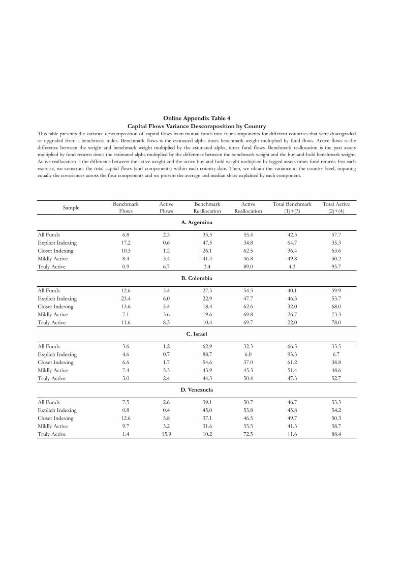
Sample Benchmark Flows

Active Flows

Benchmark Reallocation

Active Reallocation

Total Benchmark (1)+(3)

Total Active (2)+(4)

All Funds 6.8 2.3 35.5 55.4 42.3 57.7Explicit Indexing 17.2 0.6 47.5 34.8 64.7 35.3Closet Indexing 10.3 1.2 26.1 62.5 36.4 63.6Mildly Active 8.4 3.4 41.4 46.8 49.8 50.2Truly Active 0.9 6.7 3.4 89.0 4.3 95.7

All Funds 12.6 5.4 27.5 54.5 40.1 59.9Explicit Indexing 23.4 6.0 22.9 47.7 46.3 53.7Closet Indexing 13.6 5.4 18.4 62.6 32.0 68.0Mildly Active 7.1 3.6 19.6 69.8 26.7 73.3Truly Active 11.6 8.3 10.4 69.7 22.0 78.0

All Funds 3.6 1.2 62.9 32.3 66.5 33.5Explicit Indexing 4.6 0.7 88.7 6.0 93.3 6.7Closet Indexing 6.6 1.7 54.6 37.0 61.2 38.8Mildly Active 7.4 3.3 43.9 45.3 51.4 48.6Truly Active 3.0 2.4 44.3 50.4 47.3 52.7

All Funds 7.5 2.6 39.1 50.7 46.7 53.3Explicit Indexing 0.8 0.4 45.0 53.8 45.8 54.2Closet Indexing 12.6 3.8 37.1 46.5 49.7 50.3Mildly Active 9.7 3.2 31.6 55.5 41.3 58.7Truly Active 1.4 15.9 10.2 72.5 11.6 88.4

D. Venezuela

Online Appendix Table 4Capital Flows Variance Descomposition by Country

This table presents the variance descomposition of capital flows from mutual funds into four components for different countries that were downgradedor upgraded from a benchmark index. Benchmark flows is the estimated alpha times benchmark weight multiplied by fund flows. Active flows is thedifference between the weight and benchmark weight multiplied by the estimated alpha, times fund flows. Benchmark reallocation is the past assetsmultiplied by fund returns times the estimated alpha multiplied by the difference between the benchmark weight and the buy-and-hold benchmark weight.Active reallocation is the difference between the active weight and the active buy-and-hold weight multiplied by lagged assets times fund returns. For eachexercise, we construct the total capital flows (and components) within each country-date. Then, we obtain the variance at the country level, imputingequally the covariances across the four components and we present the average and median share explained by each component.

A. Argentina

B. Colombia

C. Israel