INTERIM GUIDELINES FOR THE CALCULATION OF THE COEFFICIENT ... · mepc.1/circ.796 annex, page 1...

$: INTERIM GUIDELINES FOR THE CALCULATION OF THE COEFFICIENT ... · mepc.1/circ.796 annex, page 1 i:\circ\mepc\01\796.doc annex interim guidelines for the calculation of the coefficient$
I:\CIRC\MEPC\01\796.doc

E

4 ALBERT EMBANKMENT LONDON SE1 7SR

Telephone: +44 (0)20 7735 7611 Fax: +44 (0)20 7587 3210

MEPC.1/Circ.796 12 October 2012

INTERIM GUIDELINES FOR THE CALCULATION OF THE COEFFICIENT fw FOR

DECREASE IN SHIP SPEED IN A REPRESENTATIVE SEA CONDITION FOR TRIAL USE

1 The Marine Environment Protection Committee, at its sixty-fourth session (1 to 5 October 2012), recognizing the need to develop guidelines for calculating the coefficient fw contained in paragraph 2.9 of the 2012 Guidelines on the method of calculation of the attained Energy Efficiency Design Index for new ships (resolution MEPC.212(63)), agreed to circulate the interim Guidelines for the calculation of the coefficient fw for decrease in ship speed in a representative sea condition for trial use, as set out in the annex. 2 Member Governments are invited to bring the annexed interim Guidelines to the attention of their Administration, industry, relevant shipping organizations, shipping companies and other stakeholders concerned for trial use on a voluntary basis. 2 Member Governments and observer organizations are also invited to provide information of the outcome and experiences in applying the interim Guidelines to future sessions of the Committee.

***

MEPC.1/Circ.796 Annex, page 1


ANNEX

INTERIM GUIDELINES FOR THE CALCULATION OF THE COEFFICIENT fw FOR DECREASE IN SHIP SPEED IN A REPRESENTATIVE SEA CONDITION

FOR TRIAL USE CONTENTS Introduction Part 1: Guidelines for the simulation for the coefficient fw for decrease in ship speed in

a representative sea condition

Appendix: Sample simulation of the coefficient fw Part 2: Guidelines for calculating the coefficient fw from the standard fw curves

Appendix 1: Sample calculation of the coefficient fw from the standard fw curves

Appendix 2: Procedures for deriving standard fw curves

INTRODUCTION The purpose of these guidelines is to provide guidance on calculating the coefficient fw, which is contained in the Energy Efficiency Design Index, in paragraph 2.9 in the 2012 Guidelines on the method of calculation of the attained Energy Efficiency Design Index for new ships (EEDI), adopted by MEPC.212(63). fw is a non-dimensional coefficient indicating the decrease in speed in a representative sea conditions of wave height, wave frequency and wind speed. fw should be determined by conducting the ship specific simulation on its performance at representative sea condition following the procedure specified in part 1: Guidelines for the simulation for the coefficient fw for decrease in ship speed in a representative sea condition. In cases where a simulation is not conducted, fw should be determined based on the standard fw curves following the procedure specified in part 2: Guidelines for calculating the coefficient fw from the standard fw curves. Sample simulation and calculation of the coefficient fw are shown in respective appendices to part 1 and part 2, and the procedures for deriving standard fw curves are shown in appendix 2 of part 2.



PART 1: GUIDELINES FOR THE SIMULATION FOR THE COEFFICIENT FW FOR DECREASE IN SHIP

SPEED IN A REPRESENTATIVE SEA CONDITION 1 General 1.1 Application 1.1.1 The purpose of these guidelines is to provide guidance on conducting the simulation to obtain the coefficient fw for an individual ship, which is contained in the EEDI. 1.1.2 These guidelines apply to ships of which ship resistance as well as brake power in a calm sea condition (no wind and no waves) is evaluated by tank tests, which mean model towing tests, model self-propulsion tests and model propeller open water tests. Numerical calculations may be accepted as equivalent to model propeller open water tests or used to complement the tank tests conducted (e.g. to evaluate the effect of additional hull features such as fins, etc., on ship's performance), with approval of the verifier for the EEDI. 1.1.3 The design parameters and the assumed conditions in the simulation to obtain the coefficient fw should be consistent with those used in calculating the other components in the EEDI. 1.1.4 fw may also be determined by the verifier's acceptance of the tank test and/or simulated data from the ship of the same type's performance in representative sea condition. 1.2 Method of calculation 1.2.1 Symbols

BP : Brake power

TR : Total resistance in a calm sea condition (no wind and no waves)

refV : Design ship speed when the ship is in operation in a calm sea condition

(no wind and no waves)

wV : Design ship speed when the ship is in operation under the representative

sea condition

waveR

: Added resistance due to waves

windR : Added resistance due to wind

D : Propulsion efficiency

S : Transmission efficiency

Subscript w refers to wind and wave sea conditions.

1.2.2 The basic procedures in calculating decrease in ship speed is shown in figure 1.1. (See section 4 for more information.)



Figure 1.1: Flow chart of calculation for the decrease in ship speed

1.2.3 Relation between the power and the decrease of ship speed is shown in figure 1.2

Figure 1.2: Relation between power and the decrease in ship speed

TR

wTTw RRR

Wind speed

windR waveR

Wave spectrum

refww VVf /

V : Speed

TR : Total resistance in calm sea condition

wR : Added resistance due to wind and waves

BP : Brake power

D : Propulsion efficiency

S : Transmission efficiency

find wV at the point where

BP at Bwref PV at wV

wR

)/( SDwTwBw VRP

refV

Subscript w refers to wind and wave

Vref Vw

fw=Vw / Vref

PB

0 V (knot)

P [kW]

PB(V) curve in a calm sea condition (no

wind and no waves)

PBw(V) curve in the representative sea condition



2 Representative sea condition

2.1 Representative sea condition 2.1.1 The representative sea condition for all ships is Beaufort 6, listed in table 2.1.

Table 2.1: Representative sea condition for all ships

Mean wind speed

Mean wind direction

Significant wave height

Mean wave period

Mean wave direction

windU (m/s) (deg) H (m) T (s) (deg)

BF6 12.6 0 3.0 6.7 0 2.1.2 The direction of wind and waves are defined as heading direction, which has the most significant effect on the speed reduction.

2.2 Wind condition 2.2.1 The mean wind speed and wind direction are given in table 2.1. 2.3 Wave condition 2.3.1 Symbols

D : Angular distribution function

E : Directional spectrum

H : Significant wave height

S : Frequency spectrum

T : Mean wave period : Angle between ship course and regular waves (angle 0(deg.) is defined

as the head waves direction)

: Mean wave direction ( = 0 (deg.))

: Circular frequency of incident regular waves

2.3.2 As ocean waves are characterized as irregular ones, the directional spectrum should be considered. 2.3.3 The significant wave height, mean wave period and mean wave direction are given in table 2.1. To obtain the mean wave period from the Beaufort scale, the following formula derived from a frequency spectrum for fully-developed wind waves is used.

HT 86.3

where, H is the significant wave height in metres and T is the mean wave period in seconds.

2.3.4 The directional spectrum ( E ) is composed of frequency spectrum ( S ) and angular

distribution function ( D ).

( , ; , , ) ( ; , ) ( ; )E H T S H T D

4

e),;(5

SB

SATHS



where, 4

2 2

4

z

ST

HA

,

4

21

z

ST

B

,

TTz 920.0

others 0

2cos

2

,

2

　　

　　

D

3 Ship condition 3.1 The assumed ship conditions yield to the 2012 Guidelines on the method of calculation of the attained energy efficiency design index for new ships (EEDI), adopted by MEPC.212(63) (EEDI calculation guidelines, hereafter), constant main engine output (75 per cent of MCR, to be consistent with the one used in the EEDI calculation guidelines), and operation in steady navigating conditions on the fixed course. 3.2 The current effect is not considered. 4 Method of calculation 4.1 General

4.1.1 The total resistance in the representative sea condition, TwR , is calculated by

adding wR , which is the added resistance due to wind and waves derived at 4.3, to the

resistance TR derived following the procedure specified in paragraph 1.1.2.

4.1.2 The ship speed wV is the value of V where the brake power in the representative

sea condition BwP equals to BP , which is the brake power required for achieving the speed

of refV in a calm sea condition.

4.1.3 Where BwP can be derived from the total resistance in the representative sea

condition TwR , the properties for propellers and propulsion efficiency ( D ) should be derived

from the formulas obtained from tank tests or an alternative method equivalent in terms of

accuracy, and transmission efficiency ( S ) should be the proven value as verifiable as

possible.

The brake power can also be obtained from the reliable self-propulsion tests.

SDTB VRP

4.1.4 The coefficient for decrease of ship speed fw is calculated by dividing wV by refV as

follows:

refww VVf / at the point where BP at Bwref PV at wV



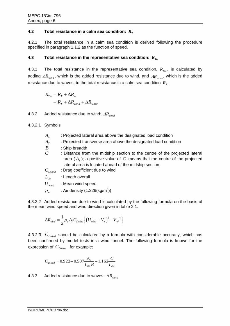
4.2 Total resistance in a calm sea condition: TR

4.2.1 The total resistance in a calm sea condition is derived following the procedure specified in paragraph 1.1.2 as the function of speed.

4.3 Total resistance in the representative sea condition: TwR

4.3.1 The total resistance in the representative sea condition, TwR , is calculated by

adding windR , which is the added resistance due to wind, and waveR , which is the added

resistance due to waves, to the total resistance in a calm sea condition TR .

wavewindT

wTTw

RRR

RRR

4.3.2 Added resistance due to wind: windR

4.3.2.1 Symbols

LA : Projected lateral area above the designated load condition

TA : Projected transverse area above the designated load condition

B : Ship breadth

C : Distance from the midship section to the centre of the projected lateral

area (LA ); a positive value of C means that the centre of the projected

lateral area is located ahead of the midship section

DwindC : Drag coefficient due to wind

OAL : Length overall

windU : Mean wind speed

a : Air density (1.226(kg/m3))

4.3.2.2 Added resistance due to wind is calculated by the following formula on the basis of the mean wind speed and wind direction given in table 2.1.

2 21

2wind a T Dwind wind w refR A C U V V

4.3.2.3 DwindC should be calculated by a formula with considerable accuracy, which has

been confirmed by model tests in a wind tunnel. The following formula is known for the

expression of DwindC , for example:

OAOA

L

DwindL

C

BL

AC 162.1507.0922.0

4.3.3 Added resistance due to waves: waveR



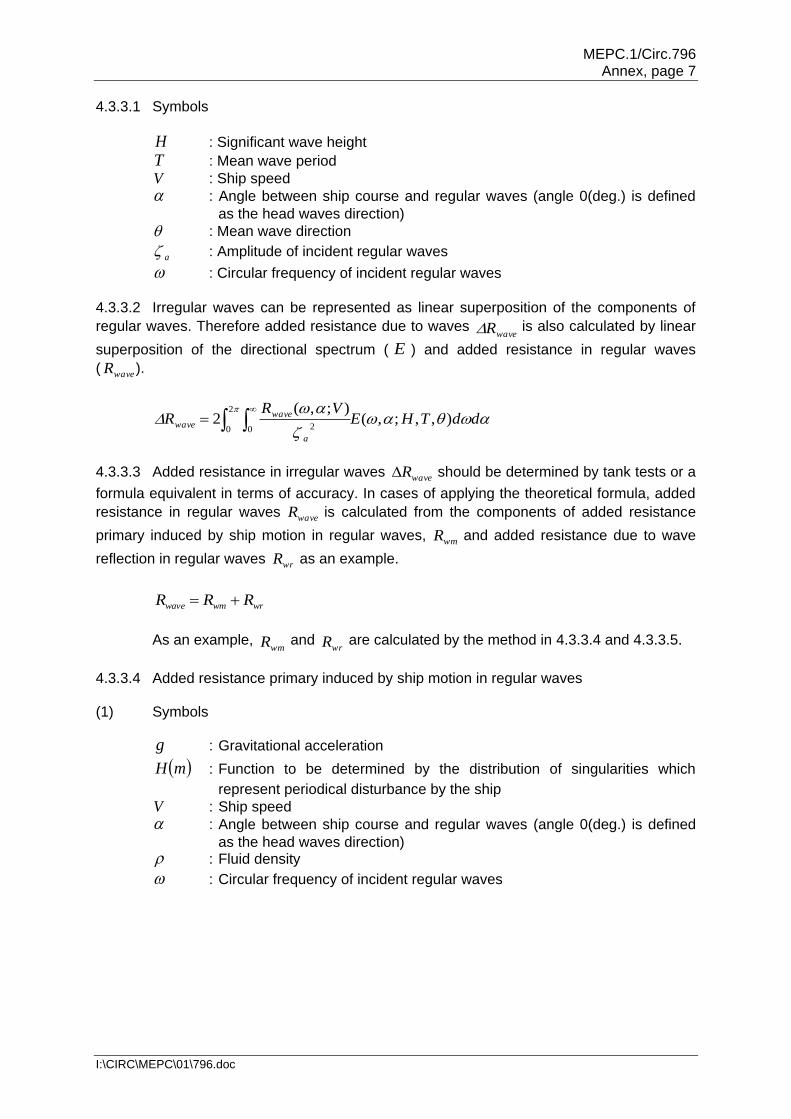
4.3.3.1 Symbols

H : Significant wave height

T : Mean wave period

V : Ship speed

: Angle between ship course and regular waves (angle 0(deg.) is defined


: Mean wave direction

a : Amplitude of incident regular waves


4.3.3.2 Irregular waves can be represented as linear superposition of the components of

regular waves. Therefore added resistance due to waves waveR is also calculated by linear

superposition of the directional spectrum ( E ) and added resistance in regular waves

( waveR ).

ddTHEVR

R

a

wave

wave ),,;,();,(

22

0 0 2

4.3.3.3 Added resistance in irregular waves waveR should be determined by tank tests or a

formula equivalent in terms of accuracy. In cases of applying the theoretical formula, added

resistance in regular waves waveR is calculated from the components of added resistance

primary induced by ship motion in regular waves, wmR and added resistance due to wave

reflection in regular waves wrR as an example.

wrwmwave RRR

As an example, wmR and

wrR are calculated by the method in 4.3.3.4 and 4.3.3.5.

4.3.3.4 Added resistance primary induced by ship motion in regular waves (1) Symbols

g : Gravitational acceleration

mH : Function to be determined by the distribution of singularities which

represent periodical disturbance by the ship

V : Ship speed


as the head waves direction) : Fluid density




(2) Added resistance primary induced by ship motion in regular waves wmR is

calculated as follows:

4

1

)(

)cos()()(4

4

1

)(

)cos()()(4

20

240

202

1

20

240

202

1

3

1

2

4

3

4

e

e

em

m

m

m

e

e

em

m

wm

dmKmKm

KmKmmH

dmKmKm

KmKmmH

R

g

Vee

,

gK

2 ,

20V

gK

cosKVe

2

41210

1

eeKm

2

41210

2

eeKm

2

41210

3

eeKm

2

41210

4

eeKm

4.3.3.5 Added resistance due to wave reflection in regular waves (1) Symbols

B : Ship breadth

fB : Bluntness coefficient, which is derived from the shape of water plane and

wave direction

UC : Coefficient of advance speed, which is determined on the basis of the

guidance for tank tests

d : Ship draft

gLVF ppn : Froude number (non-dimensional number in relation to ship

speed) g : Gravitational acceleration

1I : Modified Bessel function of the first kind of order 1

K : Wave number of regular waves

1K : Modified Bessel function of the second kind of order 1

ppL : Ship length between perpendiculars

V : Ship speed



d : Effect of draft and frequency

: Fluid density

a : Amplitude of incident regular waves




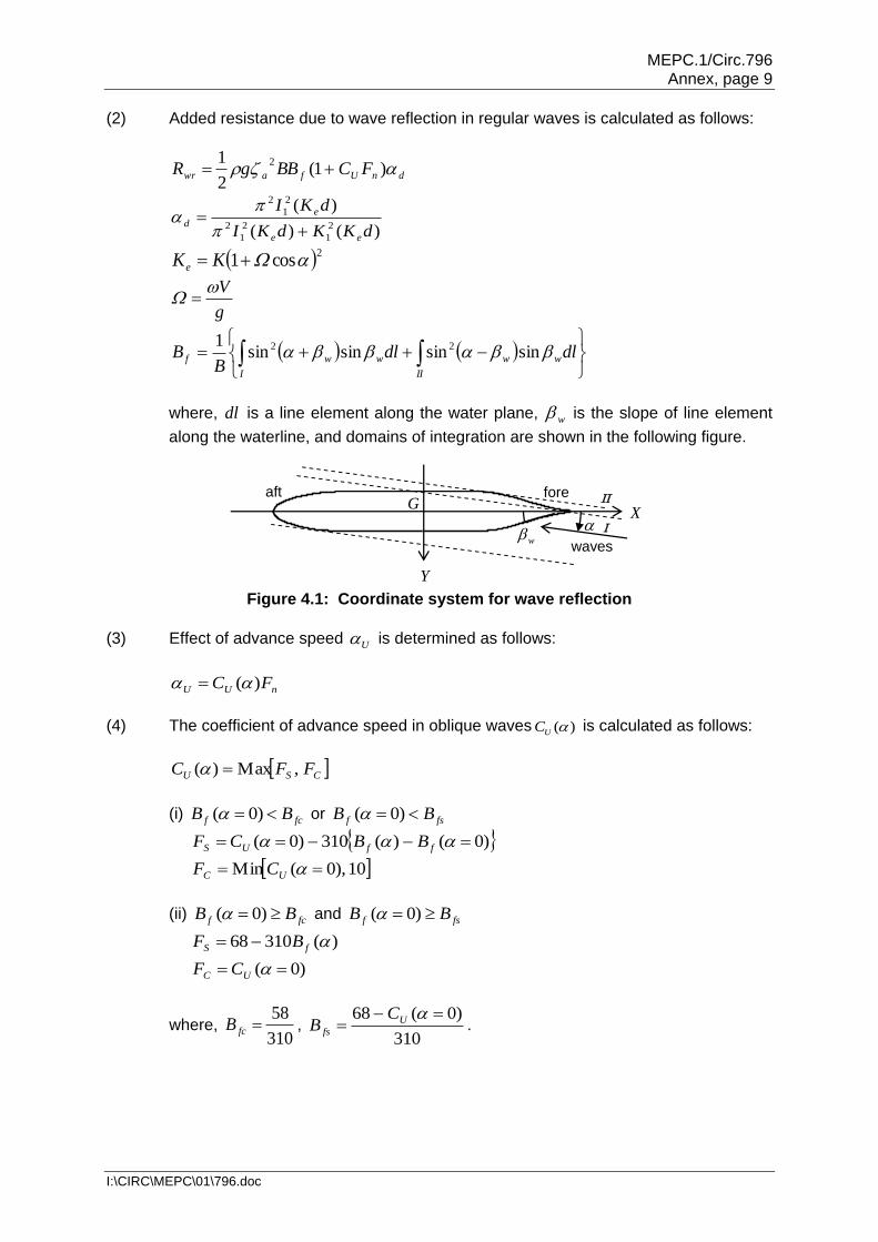
(2) Added resistance due to wave reflection in regular waves is calculated as follows:

dnUfawr FCBBgR )1(2

1 2

)()(

)(2

1

2

1

2

2

1

2

dKKdKI

dKI

ee

e

d

2cos1 KKe

g

V

II

ww

I

wwf dldlB

B sinsinsinsin1 22

where, dl is a line element along the water plane, w

is the slope of line element

along the waterline, and domains of integration are shown in the following figure.

wwaves

I

II

Y

XG

fore aft

Figure 4.1: Coordinate system for wave reflection

(3) Effect of advance speed U is determined as follows:

nUU FC )(

(4) The coefficient of advance speed in oblique waves )(UC is calculated as follows:

CSU FFC ,Max)(

(i) fcf BB )0( or fsf BB )0(

)0()(310)0( ffUS BBCF

10),0(Min UC CF

(ii) fcf BB )0( and fsf BB )0(

)(31068 fS BF

)0( UC CF

where, 310

58fcB ,

310

)0(68

U

fs

CB .



(5) The aforementioned coefficient )0( UC is determined by tank tests. The tank

tests should be carried out in short waves since wrR mainly works in short waves. The

length of short waves should be 0.5 ppL or less.

(6) Effect of advance speed in regular head waves U is calculated by the following

equation where EXP

waveR is added resistance obtained by the tank tests in regular head waves,

and wmR is added resistance due to ship motion in regular waves calculated by 4.3.3.4.

1

2

1

)()()(

2

dfa

nwmn

EXP

nUnU

BBg

FRFRFCF wave

(7) Effect of advance speed U is obtained for each speed of the experiment by the

aforementioned equation. Thereafter the coefficient of advance speed )0( UC is

determined by the least square method against nF ; see figure below. The tank tests should

be conducted under at least three different points of nF . The range of nF should include

the nF corresponding to the speed in a representative sea condition.

Figure 4.2: Determination of the coefficient of advance speed

* * *

ship speed in the

representative sea

condition in this

range

nUU FC

0 nF



APPENDIX

SAMPLE SIMULATION OF THE COEFFICIENT fw Sample: Bulk carrier The subject ship is a bulk carrier shown in the following figure and the following table.

Figure 1: Subject ship

Table 1: Dimensions of the subject ship

Dimensions Value

Length between perpendiculars 217 m

Breadth 32.26 m

Draft 14 m

Ship speed 14.5 knot

Output power at MCR 9,070 kW

Deadweight 73,000 ton

Calculation of fw from the ship specific simulation The definition of symbols and paragraph number are followed by the Guidelines for the simulation for the coefficient fw for decrease in ship speed in a representative sea condition.

1 The total resistance in a calm sea condition TR is derived from tank tests* in a calm

sea condition as the function of speed following paragraph 4.2 as shown in the following figure.

* The tank tests are conducted in the conventional ship design process for the evaluation of ship performance in a calm sea condition.

0

100

200

300

400

500

600

700

800

0 5 10 15 20

V [knot]

R T [kN]

Figure 2: Resistance in a calm sea condition

2 The added resistance due to wind windR is calculated following paragraph 4.3.2.

For the subject ship, the drag coefficient due to wind DwindC is calculated as 0.853.



3 In the guidelines, the added resistance in regular waves waveR is calculated from the

components of added resistance primary induced by ship motion in regular waves wmR and

the added resistance due to wave reflection in regular waves wrR .

wmR and wrR are calculated in accordance with paragraphs 4.3.3.4 and 4.3.3.5, respectively.

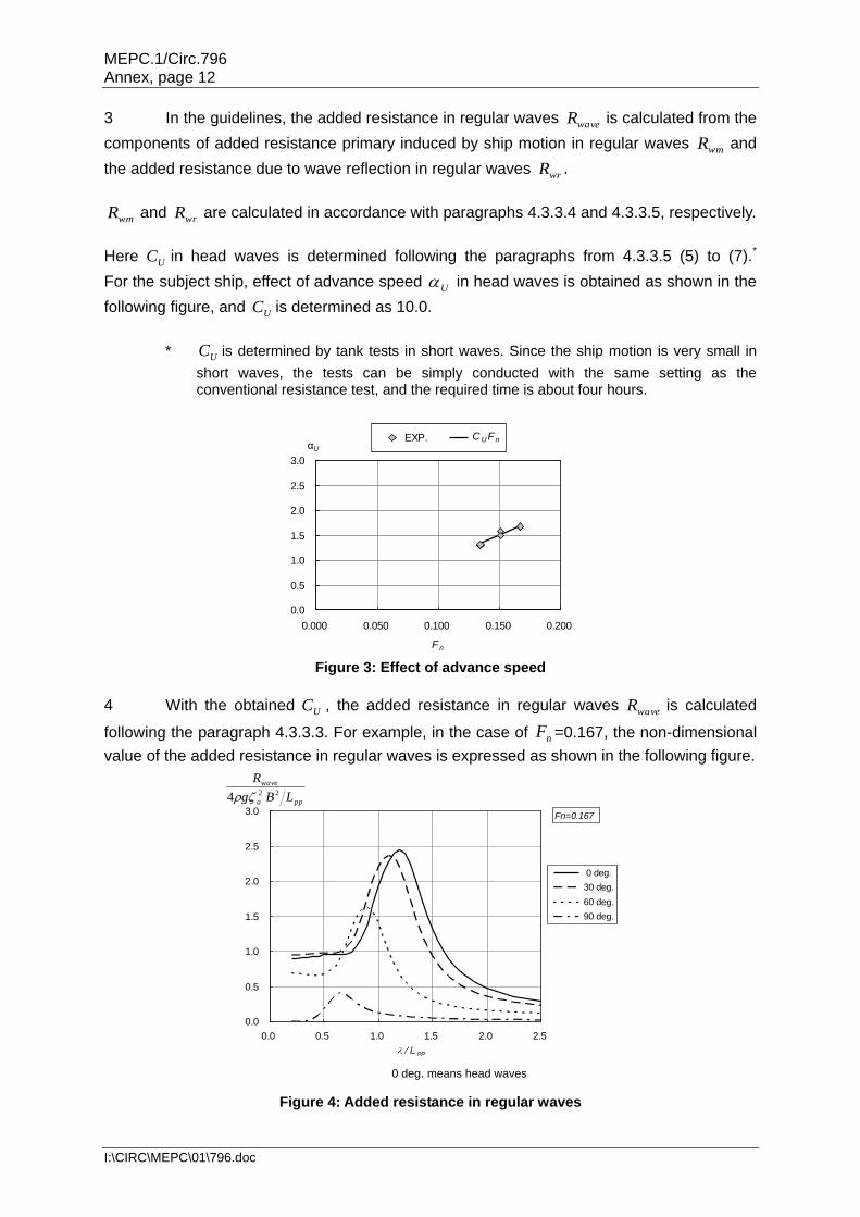
Here UC in head waves is determined following the paragraphs from 4.3.3.5 (5) to (7).*

For the subject ship, effect of advance speed U in head waves is obtained as shown in the

following figure, and UC is determined as 10.0.

* UC is determined by tank tests in short waves. Since the ship motion is very small in

short waves, the tests can be simply conducted with the same setting as the conventional resistance test, and the required time is about four hours.

0.0

0.5

1.0

1.5

2.0

2.5

3.0

0.000 0.050 0.100 0.150 0.200

F n

αU

EXP. CUFnC U F n

Figure 3: Effect of advance speed

4 With the obtained UC , the added resistance in regular waves waveR is calculated

following the paragraph 4.3.3.3. For example, in the case of nF =0.167, the non-dimensional

value of the added resistance in regular waves is expressed as shown in the following figure.

0.0

0.5

1.0

1.5

2.0

2.5

3.0

0.0 0.5 1.0 1.5 2.0 2.5

0 deg.

30 deg.

60 deg.

90 deg.

Fn=0.167

0 deg. means head waves

Figure 4: Added resistance in regular waves

ppa

waveAW

LBg

RK

224



5 The added resistance due to waves in head waves waveR is calculated following

paragraph 4.3.3.2. waveR in head waves at T = 6.7 (s) (BF6) is expressed as shown in the

following figure. For obtaining the power curve, waveR is expressed as a function of ship

speed from the calculated waveR at several ship speeds. In the sample calculation, waveR

is expressed as a quartic function of ship speed.

0.00

0.02

0.04

0.06

0.08

0.10

0 0.05 0.1 0.15 0.2

F n

pp

wave

LBgH

R228

T =6.7[s]

Figure 5: Added resistance due to waves

6 The total resistance in the representative sea condition TWR is calculated following

paragraph 4.3, and the brake power in the representative sea condition BWP is calculated

following paragraph 4.1.3. That is, TWR is calculated as a sum of TR , windR , and waveR as

shown in the following figure and BWP is calculated by dividing VRTW by the propulsion

efficiency in the representative sea condition Dw and the transmission efficiency S .



BF6

0

200

400

600

800

1000

1200

1400

0 5 10 15 20

V [knot]

R [kN]

Rt

Rt+Drwind

Rt+Drwind+Drwave

R T

R T+ R wind

R T+ R wind + R wave

Figure 6: Total resistance in the representative sea condition

7 The self-propulsion factors and the propeller characteristics for the subject ship are

shown in the following figures. Here ( w1 ) is the wake coefficient in full scale, ( t1 ) is the

thrust deduction fraction, R is the propeller rotative efficiency, nDVJ a is the advance

coefficient, aV is the advance speed of the propeller, n is the propeller revolutions, D is the

propeller diameter, TK is the propeller thrust coefficient, and QK is the propeller torque

coefficient.

8 The propulsion efficiency D is expressed as follows:

oRDw

t

1

1

where O is the propeller efficiency in open water obtained by the propeller

characteristics.

(1-w ), (1-t ), R

0.0

0.2

0.4

0.6

0.8

1.0

1.2

0 5 10 15 20

V [knot]

(1-w) (1-t) ηR

0.0

0.2

0.4

0.6

0.8

1.0

0.0 0.5 1.0 1.5

J

KT

10KQ

K T , 10K Q

Figure 7: Self-propulsion factors Figure 8: Propeller characteristics



9 The power curve in the representative sea condition is obtained by solving the equilibrium equation on a force in the longitudinal direction numerically. The representative sea condition is BF6. The brake power in a calm sea condition (BF0) and that in the representative sea condition (BF6) are calculated as shown in the following figure.

0

2000

4000

6000

8000

10000

12000

14000

16000

10 11 12 13 14 15 16

V (knot)

BF0

BF6

75%MCR

heading weather conditionBHP (kW)

V w V ref

Figure 9: Power curves

10 Following paragraph 4.1.4, the coefficient of the decrease of ship speed fw is

calculated as 0.846 from wV = 12.10(knot) and refV = 14.31(knot) at the output power

of 75 per cent MCR: 6802.5(kW). In the EEDI Technical File, fw is listed as follows:

7.2 Calculated weather factor, fw

fw 0.846



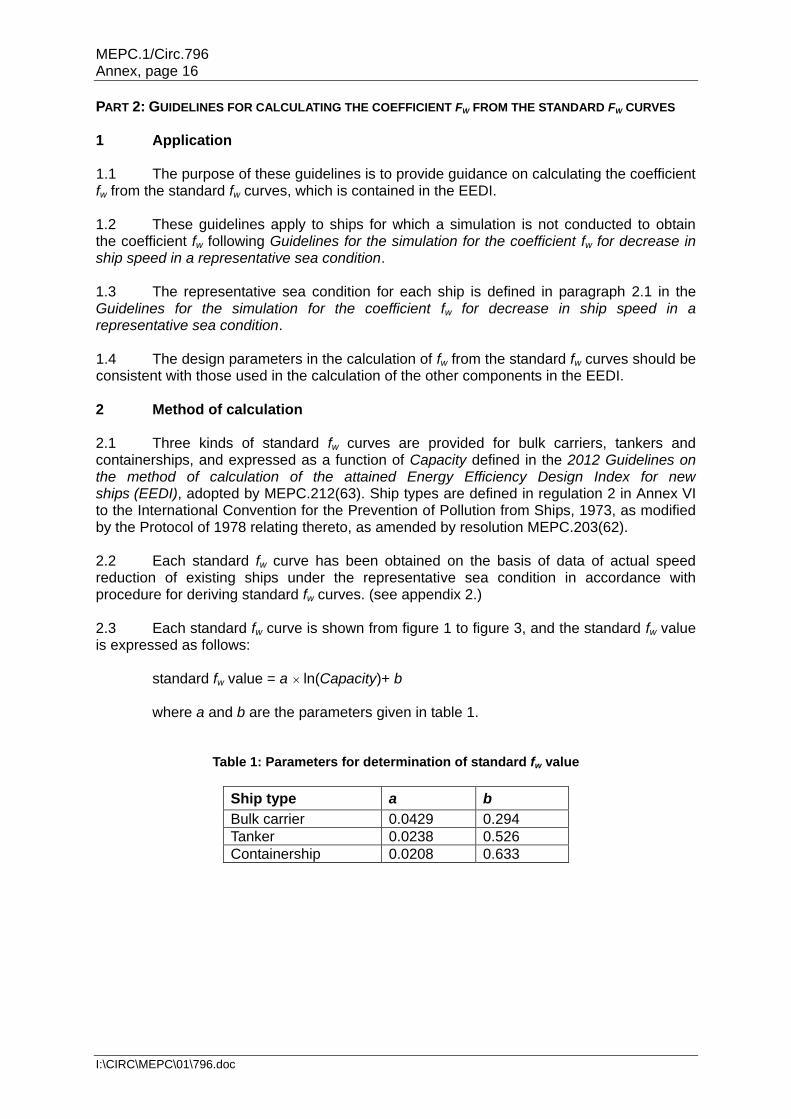
PART 2: GUIDELINES FOR CALCULATING THE COEFFICIENT FW FROM THE STANDARD FW CURVES 1 Application 1.1 The purpose of these guidelines is to provide guidance on calculating the coefficient fw from the standard fw curves, which is contained in the EEDI. 1.2 These guidelines apply to ships for which a simulation is not conducted to obtain the coefficient fw following Guidelines for the simulation for the coefficient fw for decrease in ship speed in a representative sea condition. 1.3 The representative sea condition for each ship is defined in paragraph 2.1 in the Guidelines for the simulation for the coefficient fw for decrease in ship speed in a representative sea condition. 1.4 The design parameters in the calculation of fw from the standard fw curves should be consistent with those used in the calculation of the other components in the EEDI. 2 Method of calculation 2.1 Three kinds of standard fw curves are provided for bulk carriers, tankers and containerships, and expressed as a function of Capacity defined in the 2012 Guidelines on the method of calculation of the attained Energy Efficiency Design Index for new ships (EEDI), adopted by MEPC.212(63). Ship types are defined in regulation 2 in Annex VI to the International Convention for the Prevention of Pollution from Ships, 1973, as modified by the Protocol of 1978 relating thereto, as amended by resolution MEPC.203(62). 2.2 Each standard fw curve has been obtained on the basis of data of actual speed reduction of existing ships under the representative sea condition in accordance with procedure for deriving standard fw curves. (see appendix 2.) 2.3 Each standard fw curve is shown from figure 1 to figure 3, and the standard fw value is expressed as follows:

standard fw value = a ln(Capacity)+ b where a and b are the parameters given in table 1.

Table 1: Parameters for determination of standard fw value

Ship type a b

Bulk carrier 0.0429 0.294

Tanker 0.0238 0.526

Containership 0.0208 0.633



fw = 0.0429ln(Capacity)+0.294

Figure 1: Standard fw curve for bulk carrier


Figure 2: Standard fw curve for tanker

(DWT)

(DWT)




Figure 3: Standard fw curve for containership

* * *

(DWT)



APPENDIX 1 SAMPLE CALCULATION OF THE COEFFICIENT fw FROM THE STANDARD fw CURVES

Sample: Bulk carrier The subject ship is a bulk carrier shown in the following figure and the following table.

Figure 1: Subject ship

Table 1: Dimensions of the subject ship

Dimensions Value

Length between perpendiculars 217 m

Breadth 32.26 m

Draft 14 m

Ship speed 14.5 knot

Output power at MCR 9,070 kW

Deadweight 73,000 ton

Calculation of fw from the standard fw curves The paragraph numbers are followed by guidelines for calculating the coefficient fw from the standard fw curves. 1 The standard fw value is calculated following paragraph 2.3. Since the subject ship is a bulk carrier, the standard fw value is obtained from the following equation. Standard fw value = 0.0429 ln(Capacity) + 0.294 2 Since the Capacity for the bulk carriers is deadweight, the Capacity for the subject ship is determined as 73,000 (ton). By substitution of 73,000 to the above equation, the standard fw value is obtained as 0.774. In the EEDI Technical File, fw is listed as follows:

7.2 Calculated weather factor, fw

fw 0.774



APPENDIX 2

PROCEDURES FOR DERIVING STANDARD fw CURVES

The procedures for calculating the standard fw curves comprise the following five steps: Step 1: To extract data from the ship's particulars The data needed for calculation are Displacement, Speed, Main Engine Output as well as RPM at NOR(normal rating). In case the necessary data for fw are not obtained, the data of the ship is not used for deriving the standard fw curves. Step 2: To extract data from the abstract log The data required are Displacement, Wind Direction (WDIR), Observed Beaufort Scale (WFOR), Measuring duration of Distlog and DistOG (HP (hours)), Distance Log (Distlog), Distance over the Ground (DistOG), Rotational Speed per minute (RPM) and Shaft Horse Power (SHP) for every 24 hours. The data for calculation of fw of individual ships are subject to screening, by following the procedures provided from (i) to (vi). The data meeting all the criteria provided from (i) to (vi) are to be used. In case the data are not extracted in the following process, the data of the ship is not used for deriving the standard fw curves. (i) Displacement should be within ±15 per cent of average displacement of the

voyages which have been reported to be close to the fully loaded condition or to the 70 per cent DWT condition in the case of a containership.11 In cases where displacement is not available, the average of draft may be used instead of the displacement.

(ii) Wind direction (WDIR): Heading (relative wind direction not exceeding ±67.5 degree).

(iii) Beaufort Scale (WFOR) for the selected data should be 2, 3 or 6.

The data under WFOR 2 and 3 are used to represent the calm sea condition (no wind and no waves), and the data under WFOR 6 are used to represent the representative sea condition.

(iv) The RPM (Rotational speed per minute) should be within ±5 per cent of the average RPM on the voyage.2

1 In reality, it is impossible to collect only the data which are under completely full load conditions.

Data deviated too much from the object displacement cannot be calibrated by the method described in step 3-1.

2 Data with RPM deviated from the average RPM may not be on the normal operational condition.

1. This document provides the procedures for deriving the standard fw curves on the basis of main ship particulars and operation data of approximately 180 existing ships in operation.

2. The coefficient fw has been obtained for individual existing ships, by selecting the data that meet certain conditions as explained below.

3. The derivation resulted in three standard fw curves for bulk carriers, tankers and containerships.



(v) SHP should be within ±20 per cent of the 75 per cent of the rated installed power (MCR). In case where SHP is not available, the fuel oil consumption may be used instead of the SHP.3

(vi) Distlog should be used under the conditions that the difference between DistOG and Distlog is within ±10 per cent of whichever is smaller.4

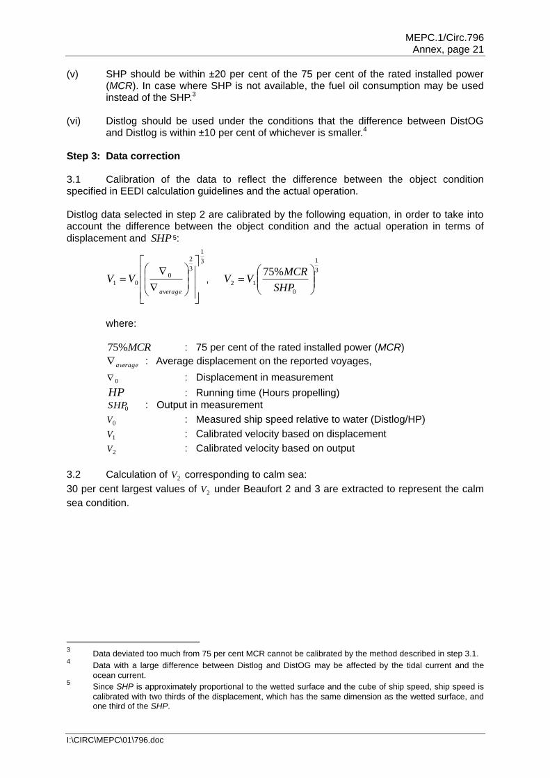
Step 3: Data correction 3.1 Calibration of the data to reflect the difference between the object condition specified in EEDI calculation guidelines and the actual operation. Distlog data selected in step 2 are calibrated by the following equation, in order to take into account the difference between the object condition and the actual operation in terms of

displacement and SHP 5:

3

1

3

2

0

01

average

VV , 3

1

0

12

%75

SHP

MCRVV

where:

MCR%75 : 75 per cent of the rated installed power (MCR)

average : Average displacement on the reported voyages,

0 : Displacement in measurement

HP : Running time (Hours propelling)

0SHP : Output in measurement

0V : Measured ship speed relative to water (Distlog/HP)

1V : Calibrated velocity based on displacement

2V : Calibrated velocity based on output

3.2 Calculation of 2V corresponding to calm sea:

30 per cent largest values of 2V under Beaufort 2 and 3 are extracted to represent the calm

sea condition.

3 Data deviated too much from 75 per cent MCR cannot be calibrated by the method described in step 3.1.

4 Data with a large difference between Distlog and DistOG may be affected by the tidal current and the

ocean current. 5 Since SHP is approximately proportional to the wetted surface and the cube of ship speed, ship speed is

calibrated with two thirds of the displacement, which has the same dimension as the wetted surface, and one third of the SHP.



Step 4: Calculation of fw for individual existing ships

fw = average of 2V corresponding to BF6 / average of 2V corresponding to calm sea for all

ships. In cases calculated fw is larger than 1.0, the data shall be removed for the averaging. Step 5: Development of "standard fw" curves Run the regression, based on the natural logarithmic function, on those fw values obtained by Step 4. Regression line, in the form of natural logarithmic line, is obtained from the observed fw values calculated in the above steps and the Capacity of each ship. The standard fw curves should be determined so that we can avoid fw by the standard curves would be much higher than the actual fw value. Then the standard fw curves are set to pass the lower limit of the observed fw values by changing the intercept of the regression line in the form of natural logarithmic line.

___________

INTERIM GUIDELINES FOR THE CALCULATION OF THE COEFFICIENT ... · mepc.1/circ.796 annex, page 1...

Documents

Transcript of INTERIM GUIDELINES FOR THE CALCULATION OF THE COEFFICIENT ... · mepc.1/circ.796 annex, page 1...