Interference and Diffraction

Two-source interference

For any two sources of the same frequency, oscillating in phase, we can explain the complex pattern of constructive and destructive interference by the same reasoning we did in 1D. At a given point, the path length difference determines whether the waves interfere constructively or destructively.

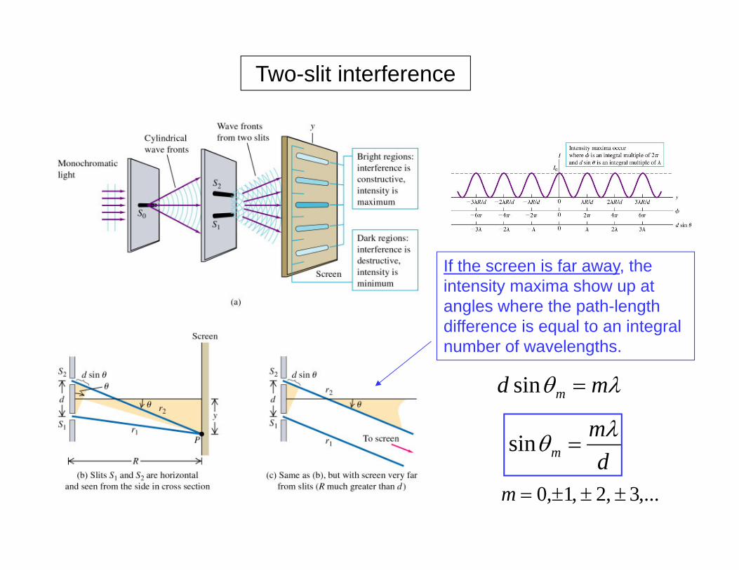
Two-slit interference

md m sin

dm

m sin

If the screen is far away, the intensity maxima show up at angles where the path-length difference is equal to an integral number of wavelengths.

,...3 ,2 ,1,0 m

Multiple-slit interference: the diffraction grating

A “diffraction grating” has many slits spaced by the same distance, d. If you pick any two slits and apply the same analysis as in the previous slide, you get the same answer for the angles of the maxima as in the two-slit case:

dm

m sin

The graphs below show that as more slits are opened, the intensity of the maxima grows as the square of the number of slits (since I is proportional to the amplitude squared). But destructive interference makes the maxima sharper, and the regions between them, darker!

Useful for spectroscopy!

Bragg diffraction of x-rays

You may be noticing that interference effects will be most observable when the wavelength of the light is comparable to the dimensions (spacings) of the thing being illuminated.Diffraction gratings can be made with spacings that are well matched to visible light (400—700 nm). X-rays are another useful region of the spectrum (10 nm and below), but diffraction gratings are not practical at this size. For x-ray wavelengths, diffraction from planes of atoms in a crystal is the practical approach: “Bragg diffraction”.

Diagram (c) below shows that for a crystal of spacing d the path length difference for reflection from two adjacent planes is 2d sin Maxima occur when this difference is an integral number of wavelengths, m:

md m sin2 m = 1,2,3,…

NaCl

(paths equal)

Edge diffraction (from Huygens’ Principle)

The photos and plots on the left show diffraction fringes caused by a laser beam passing by an edge (above), and corner (below), of a razor blade. The graph is an intensity scan of the upper photo.

To the right, is an artist’s rendition of a plane wave passing by an edge. Along the wave front near the edge, Huygens’ wavelets constructively interfere along the indicated lines. A some of the light passes around the edge into the shadow region (classically “forbidden”)—as indicated by the top arrow. The lower photo shows this same effect of waves entering a shadow region, in a ripple tank.

blad

e

blade

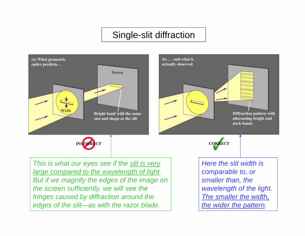
Single-slit diffraction

This is what our eyes see if the slit is very large compared to the wavelength of light. But if we magnify the edges of the image on the screen sufficiently, we will see the fringes caused by diffraction around the edges of the slit—as with the razor blade.

Here the slit width is comparable to, or smaller than, the wavelength of the light. The smaller the width, the wider the pattern.

Single-slit diffraction (from Huygens’ Principle)

Huygens

This shows how the pattern changes with slit width. If the slit width is much larger than the wavelength of light (left), plane waves emerge from the slit, with diffraction effects (fringes) at the edges. If the slit width is much smaller than the wavelength of the light (right), the slit acts as a Huygens line source, and cylindrical wave fronts are created.

Computer simulationRipple tank

Single-slit diffraction: positions of the minima

Consider the light from a strip near the top of the slit, interfering with light from a strip at a/2. Destructive interference occurs when the distance difference is half a wavelength. So there will be a dark fringe at the two positions:

2sin

2

ad

am

m sin ,...3 ,2 ,1 m

If we take this pair and sweep it from top to bottom within the slit, we see that this applies to the whole slit. Then if we choose other intervals—a/4, a/6, a/8, etc.—these would destructively interfere when |d| = to give, finally:

Diffraction patterns similar to the single slit

Square hole:

Round hole: (Airy function)

Small hole

Large hole

D 22.1sin 1

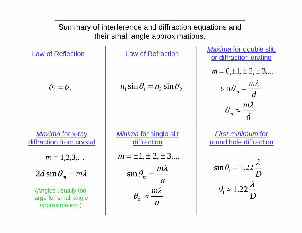
Summary of interference and diffraction equations and their small angle approximations.

D 22.1sin 1

am

m sin

,...3 ,2 ,1 m

md m sin2

m = 1,2,3,…

dm

m sin2211 sinsin nn

Maxima for double slit, or diffraction grating

Maxima for x-ray diffraction from crystal

Minima for single slit diffraction

First minimum for round hole diffraction

Law of RefractionLaw of Reflection

,...3 ,2 ,1,0 m

ri

dm

m

am

m D

22.11 (Angles usually too large for small angle

approximation.)

How to analyze interference and diffraction problems that involve minima or maxima projected on a screen.

The equations we have for single slits, double slits, diffraction gratings, and crystal diffraction are in terms of angles of rays coming from the interfering system. But often, in homework problems and in the laboratory, measurements are made on a screen placed at some distance, D. The angles are related to screen measurements as follows:

y

D

Min or max of intensityDy

tan

tanDy

Dy1tan

)(sinsin 1

Essentially, use:

If given y, then:

Then take the sine, and insert into the diffraction equation.

If given m, etc., then:

Find sin from the diffraction equation and project to the screen with then

For small angles, life is much simpler, since sin tan :then y/D, and sin in any diffraction equation!

Thin film interference

Assigned as a homework problem for extra credit

Standing waves

Here’s a picture of a standing wave as a function of time:

An electromagnetic wave encountering a conducting surface has E=0 (a node) at the surface:

The standing wave patterns above apply both to (1) strings tied between walls and to (2) E, for electromagnetic waves between conducting surfaces. There is a node at the each end. The number of nodes increases by one for each increase in f.

Frequencies of standing waves

The picture at the right shows the connection between the length of a “cavity”, L, and the wavelengths that can fit into it with one a node at each end. We let n be the index associated with each frequency, with n=1being the lowest frequency, f1, and find the allowed frequencies:

Ln n 2

nL

n2

Lcncf

nn 2

,...3,2,1n

The boundary conditions at the walls have restricted the possible frequencies to a particular set of values. This always happens in standing wave problems: the boundary conditions define the spectrum. We will see this again when we look

at the description of the hydrogen atom in basic quantum mechanics.

Discuss microwaves ovens with rotating tables.

Dispersion

We have been assuming that the index of refraction of a given material is a constant. But in reality the index of refraction for any transparent material varies as a function of wavelength, as shown in this graph. As you can see, the behavior is material-dependent, but the trend is that n decreases as increases. This means that, since v = c/n, red light travels slightly faster than blue light in these materials. And, if we look at the Law of Refraction, we see that light going from air into glass (and back) will bend less if the index of refraction is lower.

We can see this effect when white light passes through a prism. White light is a mix of all wavelengths in the visible spectrum. Light in the red portion of the spectrum will be bent less than light in the blue, leading to the dispersion (spreading) of colors into a “rainbow” spectrum: ROYGBIV.

Dispersion by water droplets in the atmosphere: rainbows.

Linearly polarized light. “Polarizer” device.Natural light, and many artificial light sources, are “unpolarized”; meaning that their polarization is randomly distributed. For linearly polarized light, the polarization axis is in the plane of the electric field (which is perpendicular to the direction in which the beam is moving).

A “polarizer” is a device that takes unpolarized light and aligns its polarization axis along a pre-selected direction top picture).

An example of a polarizer is polaroid film, which selectively absorbs any component of the electric vector in one direction and transmits the remainder—which then must be aligned with its own “polarization axis” (bottom picture). The light intensity drops by a factor of 2 in this process, because of the absorption. But, the outgoing beam has been linearly polarized.

Aligned, long-chain, polymers formed by extrusion. Dichroic (conducting along molecule axes). Biological systems.

Polarizer, followed by an “analyzer” (same device)

A “polarizer” may also serve as an “analyzer”. Among other things, it may be used to determine the direction in which light is polarized.

In the apparatus shown here, if the analyzer axis is parallel to the polarizer axis, all light is transmitted. If the analyzer axis is perpendicular to the polarizer axis, all light is blocked.

We can derive the equation for the intensity of the light that is transmitted for any angle between the polarizer and analyzer ( in the picture). The light has been polarized in the direction of E. The component along the direction of the analyzer axis is E cosFrom this, we can find the transmitted intensity as a function of angle.

20cEI pol

2220

20 coscos)cos( polan IcEEcI

This simple result is the “Law of Malus”. Sketch I as a function of !

Demo

The advantage of polarized sun glasses

Unpolarized light reflecting off a surface becomes partially polarized parallel to the surface. (100% at the Brewster angle.) Sun glasses with polaroid lenses have the polarization axes vertical, to block light with horizontal polarization, and reduce glare from horizontal surfaces. If you have polaroid sunglasses, try tilting your head by 90 degrees when you are outside, and notice the change in the glare from horizontal surfaces, such as streets.

Electromagnetic radiation

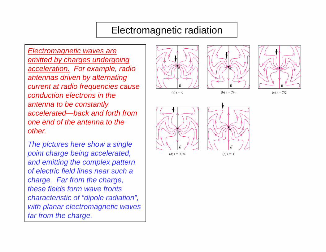
Electromagnetic waves are emitted by charges undergoing acceleration. For example, radio antennas driven by alternating current at radio frequencies cause conduction electrons in the antenna to be constantly accelerated—back and forth from one end of the antenna to the other.

The pictures here show a single point charge being accelerated, and emitting the complex pattern of electric field lines near such a charge. Far from the charge, these fields form wave fronts characteristic of “dipole radiation”, with planar electromagnetic waves far from the charge.