Document de travail du LEM 2009-17

INTERBANK OFFERED RATE: EFFECTS OF THE

FINANCIAL CRISIS ON THE INFORMATION CONTENT OF THE FIXING

Vincent Brousseau*, Alexandre Chailloux**, Alain Durré***

*IESEG School of Management, Catholic University of Lille

**International Monetary Fund ***IESEG School of Management, LEM-CNRS (UMR 8179), Catholic University of Lille

Interbank Offered Rate: Effects of the financial crisis on the information content of the fixing1

Vincent Brousseau2

Alexandre Chailloux3

Alain Durré4*

4 December 2009

Abstract With the onset of the financial turmoil in August 2007, pricing references on the money market interest rates have been shocked. The segment of unsecured deposit transactions, which represent the cornerstone of capital markets, and is used as basis for the setting of money market benchmark essential to the indexing of trillions of derivative contracts and loans, has been particularly damaged by the surge in counterparty risk. The lack of confidence between traders and the growing fear of counterparty’s bankruptcies have led progressively to a drying out of the unsecured market turnover. After a relative improvement in early 2008, market activity in the unsecured market has again dried up with the reinforcement of the financial crisis following the collapse of Lehman Brothers. Although there are good reasons to think that market activity in the cash unsecured segment of the money market has remained distorted, in particular for maturities beyond the very short-term, the OIS-LIBOR spreads have been declining extremely steadily since January 2009, both in major currencies and at various maturities, seemingly pointing to a normalization of the money market. On the basis of a simple econometric approach supported by statistical evidence applied to the euro area data, this paper analyses whether recent developments in the unsecured interest rates actually support a diagnosis of renewed market activity, and of normalization of the unsecured market. Key words: LIBOR, EURIBOR, secured segment, fixings, market distortions, financial crisis JEL Classification: G01, G14, C02, C32

1 The views expressed herein in this paper are those of the authors exclusively and do not necessarily reflect the views of the institutions to which the authors are affiliated and should not be attributed to the IMF, its Executive Board, or its management. 2 Visiting scholar at IESEG-School of Management (Lille Catholic University. 3 International Monetary Fund. 4 Lille Catholic University, IESEG-School of Management (Lille Catholic University) and LEM-CNRS (U.M.R. 8179). * Send all correspondences to a.durre@ieseg.fr.

2

1. Introduction

One of the key features of the current financial crisis is the confidence crisis it has involved in the money markets around the world. Whereas nobody questioned the access to market in both secured and unsecured segments before August 2007, uncertainties about financial soundness of credit institutions have rapidly made market participants realising that access to market liquidity could not be given for granted. Through growing use of scoring by banks, and given the importance of bilateral trade in the money market, trading in the money market in general, in the unsecured segments in particular, have reduced in total volume and narrowed to smaller groups of institutions depending on the maturity of the trade. However, the LIBOR (or Euribor)-OIS spread has been used since the beginning of the money market turmoil, as the main yardstick to illustrate the funding stress staged by commercial banks. The early stage of the crisis triggered upward pressures on interest rates across all segments of the unsecured money market. The surge in the overnight interest rates observed at the beginning of August 2007 has triggered early action by central banks that have rapidly permitted to tame the shorter end of the curve, and to put the overnight rates back in line with key rates. Since then overnight rates, albeit more volatile, have remained broadly under control, thanks to the compelling actions of central banks that have accommodated the surge in the demand for reserves at the end of maintenance periods while limiting the downward pressure on rates later in the maintenance period. This pro-active liquidity management by central banks has permitted to stabilize the short-end of the market, and as a consequence, the expectations of stable short-term rates going forward. These stable expectations explain why EONIA term swap rates have since then remained relatively unaffected by the turmoil, and adjusted swiftly to the monetary policy adjustments observed in the US and the UK. Conversely, Euribor and LIBOR rates for G10 currencies have been more volatile, and staged upward pressures that have only temporarily receded markedly following central banks’ unconditional commitment to provide unlimited liquidity across maturities.

3

Figure 1 – LIBOR-OIS spreads at 3-month maturity (in basis points)

0

0,5

1

1,5

2

2,5

3

3,5

4

01/0

6/20

07

01/0

8/20

07

01/1

0/20

07

01/1

2/20

07

01/0

2/20

08

01/0

4/20

08

01/0

6/20

08

01/0

8/20

08

01/1

0/20

08

01/1

2/20

08

01/0

2/20

09

01/0

4/20

09

01/0

6/20

09

01/0

8/20

09

01/1

0/20

09

EUR3M USD3M GBP3M

Source: Reuters and authors’ calculation

Initially seen aimed at stabilizing the short-end of the money market, central bank actions have been more and more openly geared towards stabilizing conditions in the term money market. The ECB has gradually re-balanced its liquidity provision towards longer-term refinancing operations up to one year tenor5, the Bank of England has increased the size of its long-term repo, and the Fed, via the TAF and the TSLF and other facilities has tried to help commercial banks to re-channel some liquidity towards the money market, through the exchange of highly liquid assets for assets whose refinancing access to the market had been closed.

Central banks have thus gradually changed their stance and tried to impact not only the shorter-end of the curve, as they do traditionally, but also term rates so as to re-establish a “normal functioning of the money market”. Some studies have tried to analyze the impact of central banks’ operations on some indicators of market liquidity stress, and notably on the LIBOR/OIS spread. Keister and McAndrews (2009) analyse the large quantity of reserves implied by the new liquidity facilities created by the Federal Reserve and discuss their potential effects on bank lending and the level of the economy. Taylor and Williams (2008) contend that the Fed operations (the Term Auction Facility) do not have an effect on this indicator of liquidity stress. The IMF (2008), using different empirical techniques (GARCH and Markow-Switching regime), conclude that central banks managed to reduce the market stress. Michaud and Upper (2008), after studying the drivers of LIBOR rates’ movements during the turmoil suggest that central banks’ operations were instrumental in the cooling-off of the LIBOR/OIS spread.

Gyntelberg and Wooldridge (2008), study the detailed modalities of money market fixings. They highlighted the potential biases related to participants’ strategic behaviour, but conclude 5 It is noticed that the 3-month, 6-month and one-year LTROs represent now around 90% of the ECB liquidity and the one-week operation, MRO, only 10%.

4

that fixings had worked well in a context of market dislocation, and that the dispersion within the dataset used to determine the references was a consequence of the market turmoil, and not a symptom of a flawed fixing process. They argued that the safeguards used to avert the risks of gaming of the index (trimming of the extremes) worked well in this context.

Although it can be easily argued that higher dispersion in quotes among surveyed banks and more volatile term spreads are normal features in crisis periods due to the prevailing uncertainties, the key issue is to know whether these crisis phenomena are also reflecting higher distortions in the market dynamics, in particular in the usual strong relationship existing between the unsecured and the key pricing reference of the money market, i.e. the Overnight Index Swap (OIS) curve. This is the main issue and it also constitutes its original contribution to the literature. Indeed, to our best knowledge, this issue has been only partly addressed by practitioners but it has not yet been treated in an analytical framework allowing robustness tests.

This paper is structured as follows. Following the introduction, Section 2 overviews briefly the evolution of banks’ funding in recent decades. Section 3 recalls the essence of the pricing relationship between instruments in the unsecured segments of the money market. Section 4 describes the data while Section 5 presents the dynamics of these segments prior to and during the two steps of the financial crisis (i.e. from August 2007 but prior to the collapse of Lehman and afterwards). Finally, Section 6 concludes.

2. Conceptual framework

2.1. Definition

The trading on the unsecured deposit market is the oldest form of interest rate trading. It is a decentralised and over-the-counter (OTC) market segment. A by-product of the trading on the deposit market is the LIBOR index calculated and published by the British Banking Association (BBA) since 1986. With the start of the euro in January 1999, the EURIBOR index calculated by the European Banking Federation, taking the succession of the continental European counterparts of the BBA, gained importance and quickly became the primary benchmark in the euro money market, while the predominance of the BBA-issued LIBORs remained undisputed for other currencies.

Libor (since 1986) and Euribor (since 1999) fixing rates are declarative reference used to provide a benchmark reference on term funding conditions for financial contracts (retail loans, wholesale banking activities, syndicated loans) but also OTC financial derivatives (Forward Rate Agreements (FRAs), short and long-term swaps, swaptions) and exchange-traded financial derivatives (future contracts, and options on those future contracts). A full description of the Libor-type fixings is featured in Gyntelberg and Wooldridge (2008).

5

However, given the purpose of this paper, it is worth highlighting the key features of this process and outlining the differences with other types of money market references (in particular actually traded indexes).

The calculation and definition of these indexes (as their composition) is presented in Annex I. These benchmarks have a key role far beyond cash markets as they serve as pricing reference for the above mentioned financial derivative instruments, among which, most importantly, the futures contracts of the LIFFE on the EURIBOR and LIBOR (the London International Financial Futures and options Exchange). Through the use of these futures contracts, LIFFE market’s participants hedge their cash market exposure, speculate upon the future direction of interest rate and run arbitrage strategies across market segments. In the long run at least, it is absolutely necessary to have enough activity in the deposit market to ensure correct pricing of the future contract, which requires the anchoring of the fixing to its notional underlying, and to avoid long-lasting disturbances in pricing dynamics. In essence the cash deposit market should be liquid enough to allow arbitragers to ensure on ongoing basis price parity between the contract and its cash equivalent.6 In the case of the EURIBOR, futures contract is currently the primary hedge tool for nearly all short-termed interest-rates financial instruments. On other currencies, future contracts with a similar design play the same role of primary hedge tool.7

Against this background, it appears crucial that a reasonable level of trading is maintained on the deposit market. Recent experience shows that, in a context of confidence crisis, liquidity may dry up on the term deposit market segment, which serves as a basis for the LIBOR/EURIBOR index calculation. Persistent and severe discontinuation of trading on the deposit market have the ability to erode, over time, the incentives or the ability for market participants to price correctly the fixings, hence implying that the EURIBOR index could loose its “physical” anchoring to the underlying market and become more a notional reference. In such circumstances, the main risk would be twofold. First, as a growing number of retail interest rates in the banking system are indexed on these fixings, any mispricing would automatically be translated in to interest rates applied to the real economy. Second, there is a risk that a sudden stop in trading the EURIBOR futures contract itself could occur, mainly because the arbitrage relationship with the cash market would be broken, which would

6 In the case of the Euribor this arbitrage is only feasible upon settlement of the contract, once a quarter for the 3-months future. At this juncture, arbitragers are able to benefit from any price discrepancy between the chain of future contract prices, and their cash equivalent Future Rate Agreements. These “cash” FRAs can be replicated by a set of simple deposit operations: for instance the 3X3 FRA, i.e. the right to lend over 3 months in 3 months, is simply replicated by the juxtaposition of a 6 month borrowing and a 3 month loan with matching value dates. Arbitrage should kick-in (in principle) whenever future contract implied rate differ too markedly from these “cash” FRA rates. Arbitrager will buy the “mispriced” future and sell the other contract, and pocket the difference upon settlement. 7 In the case of Germany, the Frankfurt-based FIBOR was shadowed by its London counterpart, the German Mark LIBOR.

6

de facto makes the futures un-hedgeable. In effect, as the fixing would be disanchored from its notional underlying, then also the derivatives cash-settled on that fixing would be subject to a disanchored evolution. The fact that the fixing, even in case it would loose its “physical” significance, would still influence related market because of the existing outstanding debt which is fixing- indexed.

Although the last possible development does not seem to have started yet as the trading volumes of the futures contract remain high since the beginning of the turmoil, it is important to question whether the fixings in the unsecured market have been distorted. In this respect, it is worth noticing that the recent strong decreases in the spreads between the Interbank Offered Rate (BOR) and the Overnight Index Swaps (OIS) have occurred in spite of any clear dearth of market activity in the unsecured money market, where turnover has remained pretty low in most currencies as described later on.

By contrast, actually traded money market benchmarks (EONIA, SONIA, Fed Fund effective) are benchmark references based on overnight rate operations only. Instead of being declarative, these references are based on actually traded volumes reported by panel banks to a calculating agent (the European Banking Federation (EBF) for which the ECB is calculating the EONIA, wire services for the Sonia and the Fed Fund). Each bank report by the end of the business day the amount and the volume weighted average rate of its realised overnight operation. There is no trimming, as the influence of outliers is – generally – reduced by the volume-weighting scheme. In addition, the risk of strategic or opportunistic behaviour of contributing banks is considerably reduced as banks have to report actually traded levels. Furthermore, individual contributions are kept anonymous, so that no signalling issues (e.g. banks borrowing higher than the posted average) arise via the index publication.

2.2. Historical perspective

In order to understand the current importance of the unsecured fixings of the money market, it appears essential to briefly review the roots of their evolution. In the 1980s and early 1990s commercial banks had a central role in financial systems, and played a re-distribution function, mainly reflecting the fact that they had a quasi monopoly in the collection of deposits. The fund industry was then nascent. For instance in Europe and in Japan, money market funds did not yet exist, and households were left with no choice but holding their balances with commercial banks. Resources collected by Financial Institutions and Pensions Funds did not necessarily found their way to the broader market, as the segmentation was high between the traditional “peer-to-peer” interbank markets and other financial institutions. Likewise security issuance as a funding instrument was less important and asset-base repo operations were used only anecdotally in the interbank market by trading desks to cover their

7

short exposure, but not as a liquidity management instrument (GC, General Collateral operations).

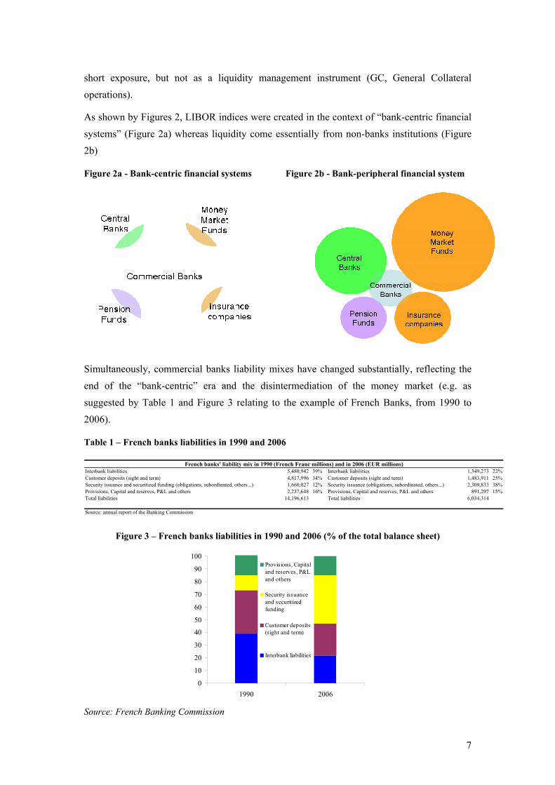
As shown by Figures 2, LIBOR indices were created in the context of “bank-centric financial systems” (Figure 2a) whereas liquidity come essentially from non-banks institutions (Figure 2b)

Figure 2a - Bank-centric financial systems Figure 2b - Bank-peripheral financial system

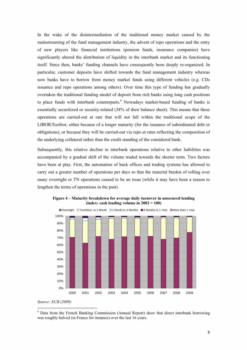
Simultaneously, commercial banks liability mixes have changed substantially, reflecting the end of the “bank-centric” era and the disintermediation of the money market (e.g. as suggested by Table 1 and Figure 3 relating to the example of French Banks, from 1990 to 2006).

Table 1 – French banks liabilities in 1990 and 2006

Interbank liabilities 5,480,942 39% Interbank liabilities 1,349,273 22%Customer deposits (sight and term) 4,817,996 34% Customer deposits (sight and term) 1,483,911 25%Security issuance and securitized funding (obligations, subordinated, others...) 1,660,027 12% Security issuance (obligations, subordinated, others...) 2,309,833 38%Provisions, Capital and reserves, P&L and others 2,237,648 16% Provisions, Capital and reserves, P&L and others 891,297 15%Total liabilities 14,196,613 Total liabilities 6,034,314

Source: annual report of the Banking Commission

French banks' liability mix in 1990 (French Franc millions) and in 2006 (EUR millions)

Figure 3 – French banks liabilities in 1990 and 2006 (% of the total balance sheet)

0

10

20

30

40

50

60

70

80

90

100

1990 2006

Provisions, Capitaland reserves, P&Land others

Security issuanceand securitizedfunding

Customer deposits(sight and term)

Interbank liabilities

Source: French Banking Commission

8

In the wake of the disintermediation of the traditional money market caused by the mainstreaming of the fund management industry, the advent of repo operations and the entry of new players like financial institutions (pension funds, insurance companies) have significantly altered the distribution of liquidity in the interbank market and its functioning itself. Since then, banks’ funding channels have consequently been deeply re-organized. In particular, customer deposits have shifted towards the fund management industry whereas now banks have to borrow from money market funds using different vehicles (e.g. CDs issuance and repo operations among others). Over time this type of funding has gradually overtaken the traditional funding model of deposit from rich banks using long cash positions to place funds with interbank counterparts.8 Nowadays market-based funding of banks is essentially securitized or security-related (38% of their balance sheet). This means that these operations are carried-out at rate that will not fall within the traditional scope of the LIBOR/Euribor, either because of a longer maturity (for the issuance of subordinated debt or obligations), or because they will be carried-out via repo at rates reflecting the composition of the underlying collateral rather than the credit standing of the considered bank.

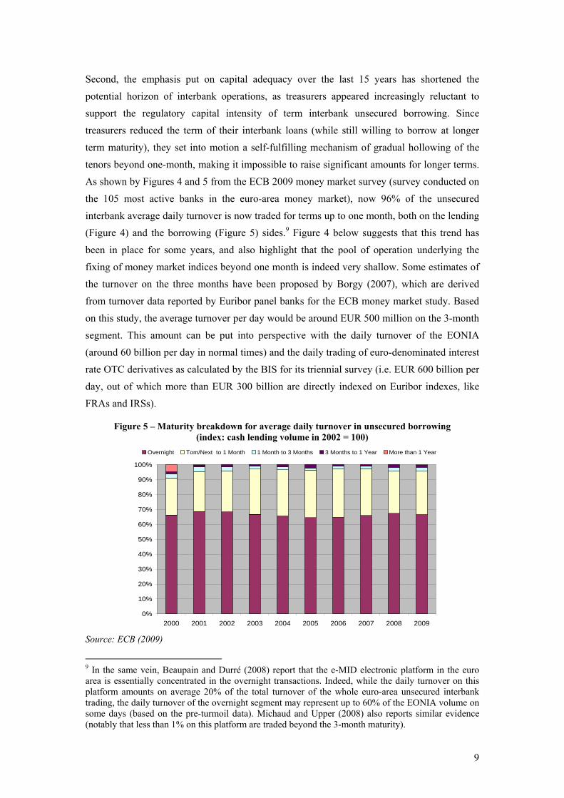
Subsequently, this relative decline in interbank operations relative to other liabilities was accompanied by a gradual shift of the volume traded towards the shorter term. Two factors have been at play. First, the automation of back offices and trading systems has allowed to carry out a greater number of operations per days so that the material burden of rolling over many overnight or TN operations ceased to be an issue (while it may have been a reason to lengthen the terms of operations in the past).

Figure 4 – Maturity breakdown for average daily turnover in unsecured lending (index: cash lending volume in 2002 = 100)

0%

10%

20%

30%

40%

50%

60%

70%

80%

90%

100%

2000 2001 2002 2003 2004 2005 2006 2007 2008 2009

Overnight Tom/Next to 1 Month 1 Month to 3 Months 3 Months to 1 Year More than 1 Year

Source: ECB (2009) 8 Data from the French Banking Commission (Annual Report) show that direct interbank borrowing was roughly halved (in France for instance) over the last 16 years.

9

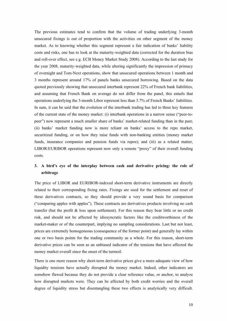
Second, the emphasis put on capital adequacy over the last 15 years has shortened the potential horizon of interbank operations, as treasurers appeared increasingly reluctant to support the regulatory capital intensity of term interbank unsecured borrowing. Since treasurers reduced the term of their interbank loans (while still willing to borrow at longer term maturity), they set into motion a self-fulfilling mechanism of gradual hollowing of the tenors beyond one-month, making it impossible to raise significant amounts for longer terms. As shown by Figures 4 and 5 from the ECB 2009 money market survey (survey conducted on the 105 most active banks in the euro-area money market), now 96% of the unsecured interbank average daily turnover is now traded for terms up to one month, both on the lending (Figure 4) and the borrowing (Figure 5) sides.9 Figure 4 below suggests that this trend has been in place for some years, and also highlight that the pool of operation underlying the fixing of money market indices beyond one month is indeed very shallow. Some estimates of the turnover on the three months have been proposed by Borgy (2007), which are derived from turnover data reported by Euribor panel banks for the ECB money market study. Based on this study, the average turnover per day would be around EUR 500 million on the 3-month segment. This amount can be put into perspective with the daily turnover of the EONIA (around 60 billion per day in normal times) and the daily trading of euro-denominated interest rate OTC derivatives as calculated by the BIS for its triennial survey (i.e. EUR 600 billion per day, out of which more than EUR 300 billion are directly indexed on Euribor indexes, like FRAs and IRSs).

Figure 5 – Maturity breakdown for average daily turnover in unsecured borrowing (index: cash lending volume in 2002 = 100)

0%

10%

20%

30%

40%

50%

60%

70%

80%

90%

100%

2000 2001 2002 2003 2004 2005 2006 2007 2008 2009

Overnight Tom/Next to 1 Month 1 Month to 3 Months 3 Months to 1 Year More than 1 Year

Source: ECB (2009)

9 In the same vein, Beaupain and Durré (2008) report that the e-MID electronic platform in the euro area is essentially concentrated in the overnight transactions. Indeed, while the daily turnover on this platform amounts on average 20% of the total turnover of the whole euro-area unsecured interbank trading, the daily turnover of the overnight segment may represent up to 60% of the EONIA volume on some days (based on the pre-turmoil data). Michaud and Upper (2008) also reports similar evidence (notably that less than 1% on this platform are traded beyond the 3-month maturity).

10

The previous estimates tend to confirm that the volume of trading underlying 3-month unsecured fixings is out of proportion with the activities on other segment of the money market. As to knowing whether this segment represent a fair indication of banks’ liability costs and risks, one has to look at the maturity-weighted data (corrected for the duration bias and roll-over effect, see e.g. ECB Money Market Study 2008). According to the last study for the year 2008, maturity-weighted data, while altering significantly the impression of primacy of overnight and Tom-Next operations, show that unsecured operations between 1 month and 3 months represent around 17% of panels banks unsecured borrowing. Based on the data quoted previously showing that unsecured interbank represent 22% of French bank liabilities, and assuming that French Bank on average do not differ from the panel, this entails that operations underlying the 3-month Libor represent less than 3.7% of French Banks’ liabilities. In sum, it can be said that the evolution of the interbank trading has led to three key features of the current state of the money market: (i) interbank operations in a narrow sense (“peer-to-peer”) now represent a much smaller share of banks’ market-related funding than in the past; (ii) banks’ market funding now is more reliant on banks’ access to the repo market, securitized funding, or on how they raise funds with non-banking entities (money market funds, insurance companies and pension funds via repos); and (iii) as a related matter, LIBOR/EURIBOR operations represent now only a remote “proxy” of their overall funding costs.

3. A bird’s eye of the interplay between cash and derivative pricing: the role of arbitrage

The price of LIBOR and EURIBOR-indexed short-term derivative instruments are directly related to their corresponding fixing rates. Fixings are used for the settlement and reset of these derivatives contracts, so they should provide a very sound basis for comparison (“comparing apples with apples”). These contracts are derivatives products involving no cash transfer (but the profit & loss upon settlement). For this reason they bear little or no credit risk, and should not be affected by idiosyncratic factors like the creditworthiness of the market-maker or of the counterpart, implying no sampling considerations. Last but not least, prices are extremely homogeneous (consequence of the former point) and generally lay within one or two basis points for the trading community as a whole. For this reason, short-term derivative prices can be seen as an unbiased indicator of the tensions that have affected the money market overall since the onset of the turmoil.

There is one more reason why short-term derivative prices give a more adequate view of how liquidity tensions have actually disrupted the money market. Indeed, other indicators are somehow flawed because they do not provide a clear reference value, or anchor, to analyze how disrupted markets were. They can be affected by both credit worries and the overall degree of liquidity stress but disentangling these two effects is analytically very difficult.

11

Furthermore, it is impossible to know which level, going forward, would represent a “normal level” once liquidity tensions will have abated10. By contrast, analyzing the efficiency of spot-forward arbitrage operations between the cash fixing and BOR-indexed derivatives should give a very precise and objective character to this debate as the pricing parity should be rigorously observed at all times in a cruise speed environment (thus providing for this “anchor”).

Forward rate agreements (FRAs) are interest rate risk instruments traded on the OTC market by counterparts willing to hedge interest rate risk, speculators willing to take exposure on interest rate movements and arbitrageurs whose operations are meant to benefit from inconsistency between prices of instruments offering similar characteristics. FRAs are straightforward instruments whose trading started with the development of modern money markets. Trading of these instruments developed rapidly on account of their potential for leveraging (the exposure is notional but there is no need to immobilize cash), the cash settlement, but also the fact that it relates to popular indexes used for the indexation of most commercial bankers assets and liabilities. FRAs also became extremely popular instruments for liquidity managers, as they allowed the building-up of interest rate exposures with little regulatory capital consumption and liquidity risks.

3.1. The FRA/LIBOR fixing pricing parity

FRAs and other short-term derivatives (interest rate swaps, future contracts) are risk management instruments mostly based on the corresponding BOR curve, so, in the case of the euro, on the EURIBOR cash curve. Although they are cash settled (these products require no settlement of the notional amount of the contract), they have a very tight relationship with the cash curve. Based on the working assumption that any market participant can borrow/lend freely at the fixing rate published daily, there ought to be a strong pricing parity between the cash curve (the master curve) and the yield curves of the related instruments. To give a trivial example, the 3X6 FRA quotations11 should be coherent with corresponding 3-month and 6-month LIBOR as simultaneously borrowing for 6 months and lending for 3 months creates a forward exposure whose break-even rates can be calculated from the two former rates (borrower for 3 months in three months). This spot-forward pricing parity used to hold because market participants, in normal times (i.e. whenever access to unsecured lending and

10 There is an ongoing debate on where the LIBOR-OIS could settle once back into a “cruise speed environment”. Some banks see a spread around 30 basis points as a possible anchor going forward. It is worth remembering that this spread had remained below 10 basis points for several years during the 90’s and at the turn of the century, highlighting that the “underpricing” of the cost of liquidity was a well-entrenched phenomenon in the last 10 years. 11 The quotation conventions read as follow: a 3X6 FRA represents the right to purchase or sell a 3- month deposit with a starting date in 3 months. A 6X9 FRA is for a 3-month deposit in 6 months, and so on.

12

borrowing is unlimited), arbitrage out any difference that would arise between FRA prices and their “theoretical fair value” derived from the cash fixing curve.

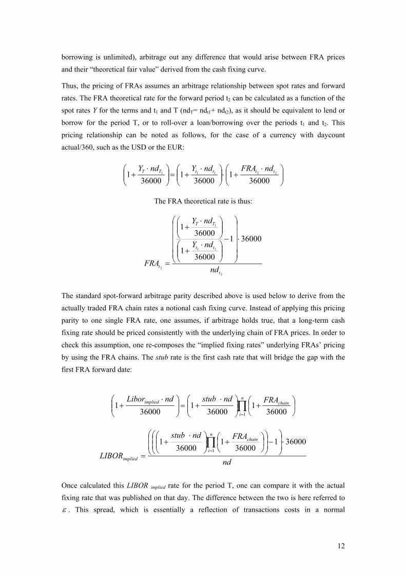
Thus, the pricing of FRAs assumes an arbitrage relationship between spot rates and forward rates. The FRA theoretical rate for the forward period t2 can be calculated as a function of the spot rates Y for the terms and t1 and T (ndT= ndt1+ ndt2), as it should be equivalent to lend or borrow for the period T, or to roll-over a loan/borrowing over the periods t1 and t2. This pricing relationship can be noted as follows, for the case of a currency with daycount actual/360, such as the USD or the EUR:

⎟⎟⎠

⎞⎜⎜⎝

⎛ ⋅+⋅⎟⎟

⎠

⎞⎜⎜⎝

⎛ ⋅+=⎟⎟

⎠

⎞⎜⎜⎝

⎛ ⋅+

360001

360001

360001 22111 ttttTT ndFRAndYndY

The FRA theoretical rate is thus:

2

11

1

2

360001

360001

360001

t

tt

TT

t nd

ndY

ndY

FRA

⋅

⎟⎟⎟⎟⎟

⎠

⎞

⎜⎜⎜⎜⎜

⎝

⎛

−

⎟⎟⎠

⎞⎜⎜⎝

⎛ ⋅+

⎟⎟⎠

⎞⎜⎜⎝

⎛ ⋅+

=

The standard spot-forward arbitrage parity described above is used below to derive from the actually traded FRA chain rates a notional cash fixing curve. Instead of applying this pricing parity to one single FRA rate, one assumes, if arbitrage holds true, that a long-term cash fixing rate should be priced consistently with the underlying chain of FRA prices. In order to check this assumption, one re-composes the “implied fixing rates” underlying FRAs’ pricing by using the FRA chains. The stub rate is the first cash rate that will bridge the gap with the first FRA forward date:

∏=

⎟⎠⎞

⎜⎝⎛ +⎟⎟

⎠

⎞⎜⎜⎝

⎛ ⋅+=⎟⎟

⎠

⎞⎜⎜⎝

⎛ ⋅+

n

i

chainimplied FRAndstubndLibor

1 360001

360001

360001

nd

FRAndstub

LIBOR

n

i

chain

implied

36000136000

136000

11

⋅⎟⎟⎠

⎞⎜⎜⎝

⎛−⎟

⎟⎠

⎞⎜⎜⎝

⎛⎟⎠⎞

⎜⎝⎛ +⎟⎟

⎠

⎞⎜⎜⎝

⎛ ⋅+

=∏=

Once calculated this LIBOR implied rate for the period T, one can compare it with the actual fixing rate that was published on that day. The difference between the two is here referred to ε . This spread, which is essentially a reflection of transactions costs in a normal

13

environment, is easy to calculate for most major currencies and for various pairs of term, e.g. on the 3-months and 6-months, or on the 6 months and one year BOR terms:

timpliedt

fixingt LIBORLIBOR ε=−

Historical data show that this pricing parity, once accounted for the small deviations between fair value and actually traded prices that related to transactions costs, or specific episodes (e.g. Y2K), was in general strictly enforced by arbitrageurs. Data starting in July 2008 show that the distance between theoretical prices and actual prices traded in the derivative market has surged to unprecedented levels (see an example in Figure 6), and this across all major currencies. LIBOR USD, GBP, EUR, and EURIBOR have been affected in the same manner by the turmoil.

Figure 6 - Value of Epsilon (ε) for the FRA 3X6 chained to deposit 3-m vs. deposit 6-m rates for

the EURIBOR (in 2007 and 2008)

-0,25

0,00

0,25

0,50

0,75

1,00

1 July 2007 1 January2008

1 July 2008 1 January2009

1 July 2009

Source: Reuters and authors’ calculation

3.2. The Information content of the spread implicit vs. actual fixings

What is the analytical value of this spread between BOR-indexed derivatives implied fixing curves and the actual fixing curve? This spread between theoretical and actual fixing represents market makers’ assessment of the cost of physically hedging the exposure (say borrowing 6 months and lending three months as in the example used above), would this exposure need to be hedged upfront or closed. In that sense it is a pure reflection of the liquidity risk faced when hedging physically a derivative position for an interbank counterpart. For this reason, this spread should increase with the overall degree of liquidity stress but also with the length of the resets on the contract. Thus, a contract with overnight

14

resets (e.g. OIS) will be deemed less “liquidity risk exposed” than a contract embedding 3- or 6-months resets, as physical hedging in the former case will require raising cash respectively for 3 and 6 months. This does explain why BOR-related derivative curve tends to show higher spreads towards the fixing curve when they embed longer resetting period. The value of this approach is that it offers somehow an unbiased measure of this “execution cost” (i.e. cost required to replicate physically the exposure achieved through BOR-related derivatives) that is a good proxy of the degree of disruption that plagued the money market.

The existence and the magnitude of this spread suggest that fixings do not only reflect funding pressure experienced by banks. It also highlights that arbitrageurs were not in a position to enter the market and take advantage of this differential, simply because like most market participants, they fell short of the type of market access12 that would have been necessary to exploit this arbitrage opportunity. Looking backward, the ease at which the implicit cash curve shifted from the actual fixing curve is easy to understand. For years arbitrageurs had ceased to be active on the spot-forward segment of the BOR indices. Instead they had shifted their focus towards placing spread bets on various segments of the money market yield curves. Anecdotal reports suggest that this spot-forward pricing relationship was extremely traded between EURIBOR-based derivatives and OIS swaps. FRAs and BOR swaps were traded against OIS used as a proxy for cash.13 Money market spreads were anchored because of the widespread belief that OIS represented the rate at which term funding was deemed to be routinely available.

12 This means that counterparts willing to lend to them at the fixing rate. 13 Instead of a pure pricing parity, arbitrageurs traded the assumption that BOR should be at least 5 to 6 basis points above OIS rates, because OIS references are actual traded rates (bid or ask depending on which counterpart took the initiative of the trade, and henceforth statistically mid-rates), while the BORs were meant to be an offered rate

15

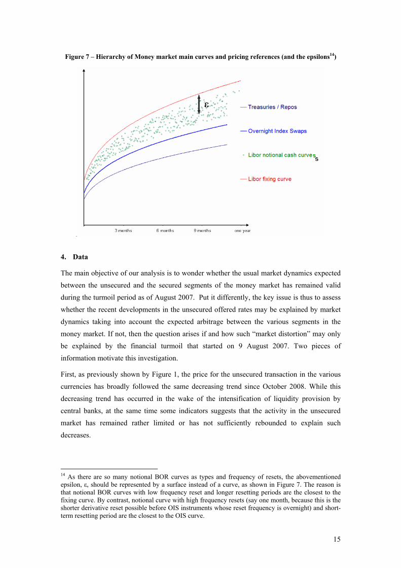
Figure 7 – Hierarchy of Money market main curves and pricing references (and the epsilons14)

4. Data

The main objective of our analysis is to wonder whether the usual market dynamics expected between the unsecured and the secured segments of the money market has remained valid during the turmoil period as of August 2007. Put it differently, the key issue is thus to assess whether the recent developments in the unsecured offered rates may be explained by market dynamics taking into account the expected arbitrage between the various segments in the money market. If not, then the question arises if and how such “market distortion” may only be explained by the financial turmoil that started on 9 August 2007. Two pieces of information motivate this investigation.

First, as previously shown by Figure 1, the price for the unsecured transaction in the various currencies has broadly followed the same decreasing trend since October 2008. While this decreasing trend has occurred in the wake of the intensification of liquidity provision by central banks, at the same time some indicators suggests that the activity in the unsecured market has remained rather limited or has not sufficiently rebounded to explain such decreases.

14 As there are so many notional BOR curves as types and frequency of resets, the abovementioned epsilon, ε, should be represented by a surface instead of a curve, as shown in Figure 7. The reason is that notional BOR curves with low frequency reset and longer resetting periods are the closest to the fixing curve. By contrast, notional curve with high frequency resets (say one month, because this is the shorter derivative reset possible before OIS instruments whose reset frequency is overnight) and short-term resetting period are the closest to the OIS curve.

16

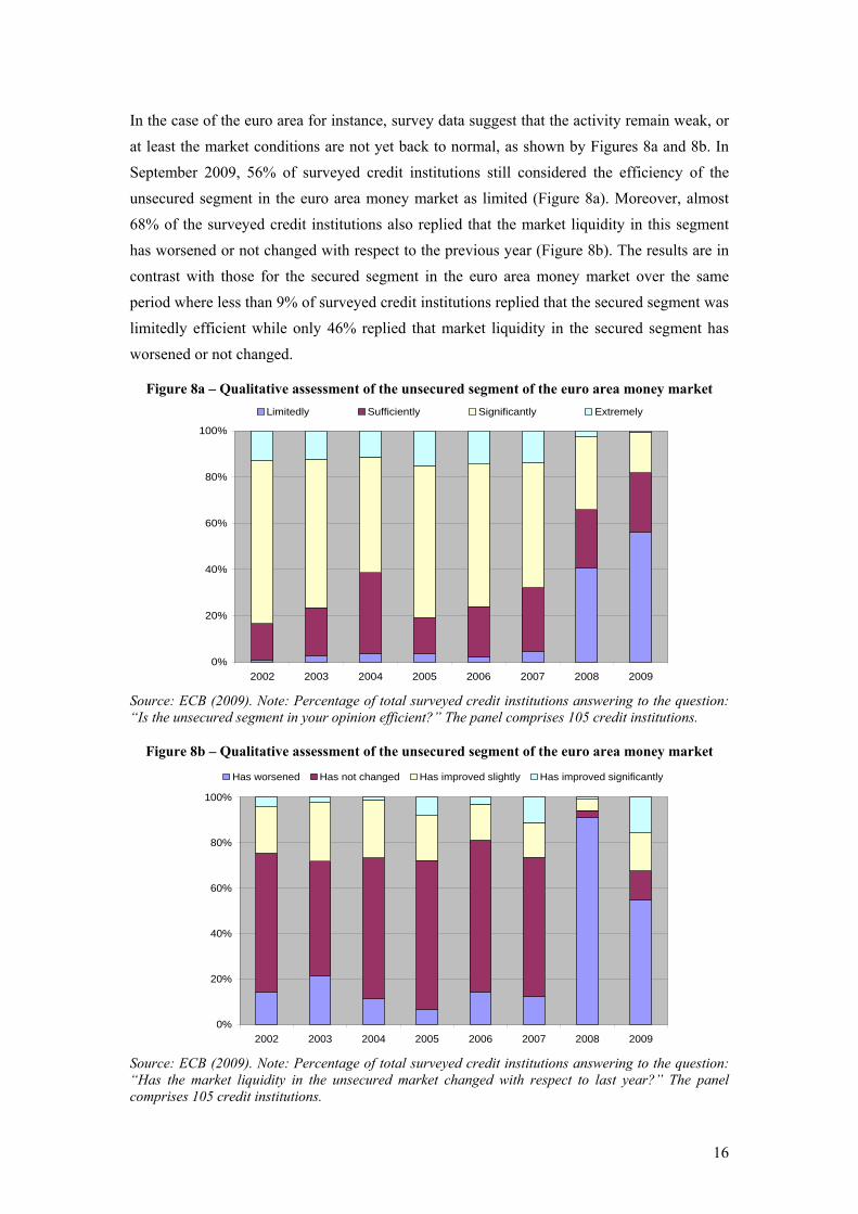
In the case of the euro area for instance, survey data suggest that the activity remain weak, or at least the market conditions are not yet back to normal, as shown by Figures 8a and 8b. In September 2009, 56% of surveyed credit institutions still considered the efficiency of the unsecured segment in the euro area money market as limited (Figure 8a). Moreover, almost 68% of the surveyed credit institutions also replied that the market liquidity in this segment has worsened or not changed with respect to the previous year (Figure 8b). The results are in contrast with those for the secured segment in the euro area money market over the same period where less than 9% of surveyed credit institutions replied that the secured segment was limitedly efficient while only 46% replied that market liquidity in the secured segment has worsened or not changed.

Figure 8a – Qualitative assessment of the unsecured segment of the euro area money market

0%

20%

40%

60%

80%

100%

2002 2003 2004 2005 2006 2007 2008 2009

Limitedly Sufficiently Significantly Extremely

Source: ECB (2009). Note: Percentage of total surveyed credit institutions answering to the question: “Is the unsecured segment in your opinion efficient?” The panel comprises 105 credit institutions.

Figure 8b – Qualitative assessment of the unsecured segment of the euro area money market

0%

20%

40%

60%

80%

100%

2002 2003 2004 2005 2006 2007 2008 2009

Has worsened Has not changed Has improved slightly Has improved significantly

Source: ECB (2009). Note: Percentage of total surveyed credit institutions answering to the question: “Has the market liquidity in the unsecured market changed with respect to last year?” The panel comprises 105 credit institutions.

17

Similar evidence is reported for the unsecured segment of the money market in the United States. For instance, the survey conducted by the ACI Financial Markets Association in June 2008 reports that 82% out of the 106 professionals replied that the unsecured segment not functioning properly, notably mentioning that some LIBOR fixings do not reflect the actual prevailing money market rates for cash (24% of these replies indicated that such phenomenon mainly concerned the USD LIBOR fixing).15 In addition, Taylor and Williams (2008) suggest developments in the spreads between the LIBOR and the OIS, when correcting for term expectations, could not be explained by liquidity provisions by the Federal Reserve, notably in the form of the credit facilities provided through the Term Auction Facility (TAF), whereas Christensen et al. (2009) find some impact.

Second, when looking at the dispersion of prices from panel banks with respect to the average price fixing, some evidence also suggests that market activity is not yet back to normal conditions. Indeed, in line with the procedure for calculation of the fixings (presented in Annex I), it is expected that panel banks report prices subject to current market conditions (i.e. the notion of “a reasonable market size”). At given market conditions and assuming reasonable level of information exchange within the market, it could be expected that the dispersion of prices from panel banks with respect to the average price remains broadly stable. Before focusing on the particular case of the euro area money market, it is interesting to observe the evolution of this dispersion of prices for the four main families of fixings, namely the EURIBOR, and the LIBOR for euro, for dollar and for sterling. In each of those four families, one finds several maturities, ranging to either overnight or 1-week, to 1-year; the most important maturities are 3-month, as the 3-month EURIBOR, the 3-month dollar Libor and the 3-month sterling LIBOR are the reference values of the principal short-term interest rates future contracts16, and the 6-month. Both the 3-month and the 6-month fixings support the standard and liquid Interest Rate Swaps (IRS).

For each fixing of the four main families at the 3-month maturity, and for every day, we construct the difference between individual banks contributions and the final published value of that fixing, and then take the standard deviation over banks which measures the dispersion of the contributions of those banks to a particular fixing. For each of the four families of fixings, we aggregate over maturities by taking the median. We hence obtain four indicators that measures the dispersion of bank’s contribution irrespective of the maturity of the fixing. To those four indicators pertaining to the EURIBOR and to the three LIBORs, we add a general indicator pertaining to the four families, also using the median.

15 Also see the results of the questionnaire on “The Functioning of Money Markets in 2008”, conducted by ACI-The Financial Markets Association with its members/traders. Results published on 18 June 2008 (see www.aciforex.com). 16 Those are the EURIBOR futures contract, the Eurodollar futures contract, and the so-called “Short Sterling”, all of which are traded at the LIFFE.

18

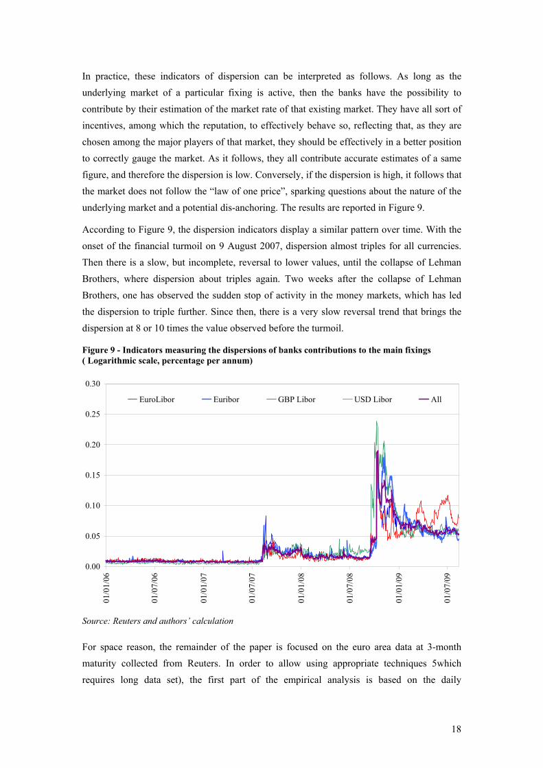
In practice, these indicators of dispersion can be interpreted as follows. As long as the underlying market of a particular fixing is active, then the banks have the possibility to contribute by their estimation of the market rate of that existing market. They have all sort of incentives, among which the reputation, to effectively behave so, reflecting that, as they are chosen among the major players of that market, they should be effectively in a better position to correctly gauge the market. As it follows, they all contribute accurate estimates of a same figure, and therefore the dispersion is low. Conversely, if the dispersion is high, it follows that the market does not follow the “law of one price”, sparking questions about the nature of the underlying market and a potential dis-anchoring. The results are reported in Figure 9.

According to Figure 9, the dispersion indicators display a similar pattern over time. With the onset of the financial turmoil on 9 August 2007, dispersion almost triples for all currencies. Then there is a slow, but incomplete, reversal to lower values, until the collapse of Lehman Brothers, where dispersion about triples again. Two weeks after the collapse of Lehman Brothers, one has observed the sudden stop of activity in the money markets, which has led the dispersion to triple further. Since then, there is a very slow reversal trend that brings the dispersion at 8 or 10 times the value observed before the turmoil.

Figure 9 - Indicators measuring the dispersions of banks contributions to the main fixings ( Logarithmic scale, percentage per annum)

0.00

0.05

0.10

0.15

0.20

0.25

0.30

01/0

1/06

01/0

7/06

01/0

1/07

01/0

7/07

01/0

1/08

01/0

7/08

01/0

1/09

01/0

7/09

EuroLibor Euribor GBP Libor USD Libor All

Source: Reuters and authors’ calculation

For space reason, the remainder of the paper is focused on the euro area data at 3-month maturity collected from Reuters. In order to allow using appropriate techniques 5which requires long data set), the first part of the empirical analysis is based on the daily

19

observations for the 3-month deposit interest rate and the 3-month overnight index swap (OIS) collected from Reuters. The second part of the empirical analysis is based on the interbank offered rates and the EONIA fixings in EUR, also provided by Reuters (see Annex I).17

5. Empirical evidence

The debate on the possible distortions in the LIBOR/Euribor fixings has been first fuelled by anecdotal information coming from other cash segments of the market, like the interest rates implied in FX swaps prices, or some pricing indications collected by brokers in the NY market by the Federal Reserve of New York (H15). Michaud and Upper (2008) have for instance shown how USD deposit rates derived from FX swaps (basis swaps) have deviated substantially from the Libor at times of liquidity stress.18 The limitation of these alternative measures is that they are affected by some idiosyncratic factors that limit the bearing of this type of analogy. Belton et al. (2008) also expressed reservations on the accuracy of these yardsticks, highlighting the impact of the time difference, and also the different sampling (H15 banks, or banks quoting the FX swaps represent a much broader and heterogeneous sample than Libor panel banks), cautioning against a premature “too low Libor” conclusion. Later on, similar doubts were expressed, although not based on proper empirical analysis but rather on anecdotal evidence. However, these criticisms made by practitioners have not yet been formally analysed with an econometric framework allowing various robustness tests, which is the main purpose of this paper.

In order to contribute to the debate, the empirical part of this paper aims at analysing the market dynamics between unsecured (deposit/EURIBOR) and the secured (OIS/EONIA fixing) segments of the euro area money market. As said previously, given the natural arbitrage between the various segments in the money markets, there is no compelling reason in theory which could explain that the unsecured rates or fixings diverge significantly from the OIS rate at any point in time. This intuition is necessarily related to the existence of arbitrage in financial markets, which is turn occurs when markets are functioning properly.

5.1. Dynamics of the time series

The first natural technique to test possible divergence in the expected strong relationship between the 3-month EURIBOR and the EONIA swap index is to look at their co-movement. In particular, it is expected that, by arbitrage, any movement in one particular time series

17 It is worth noting that there also exists a LIBOR in euro provided by the British Banking Association (BBA) and based on panel banks which are not necessarily those of the panel banks surveyed by the EBF, which is also reported in Figure XXX. Indeed, the BBA’s panel for the LIBOR in euro contains 16 banks against 45 panel banks for the EURIBOR (see Tables A.1 and A.2 in Annex I). 18 Some similar deviations have also been observed between the deposit rates and the EURIBOR fixings on some days during 2007-2008, although of moderate magnitude (see Chadha and Durré, 2009).

20

should be shortly followed by a similar movement in the other time series and vice-versa. Put it differently, there should exist between these two variables a strong and stable relationship in the long run, assuming efficient functioning of the money market.

Implicitly referring to the cointegration technique, we suggest here to proceed in two steps. First, displaying both the same stochastic process of order I(1)19, we test whether both times series has a relationship of the type (1,-1) where their joint variation is equal to a constant. Second, we check whether this relationship may have changed across sub-samples distinguishing the pre- and the turmoil periods.

For this purpose, we first use the daily data for the 3-month (unsecured) deposit rate and the 3-month OIS swap for the euro area from 4 January 1999 to 28 September 2009, i.e. 2749 observations.

In order to test the relationship between the 3-month deposit rate and the 3-month OIS, the following univariate equation is run:

tm

tm

t OISDEP εβα ++= 33 (1)

where mtDEP3 represents the 3-month deposit interest rate, m

tOIS 3 is the 3-month interest swap while α and tε are respectively a time-invariant intercept and the residuals. In

presence of arbitrage and existing markets, it is expected that the intercept, referring here to the possible spread between both financial instruments, takes a positive value and hence being statistically and significantly different from zero whereas it is also expected that the estimated coefficient, β , of the variable m

tOIS 3 is significantly equal to one. Since both variables

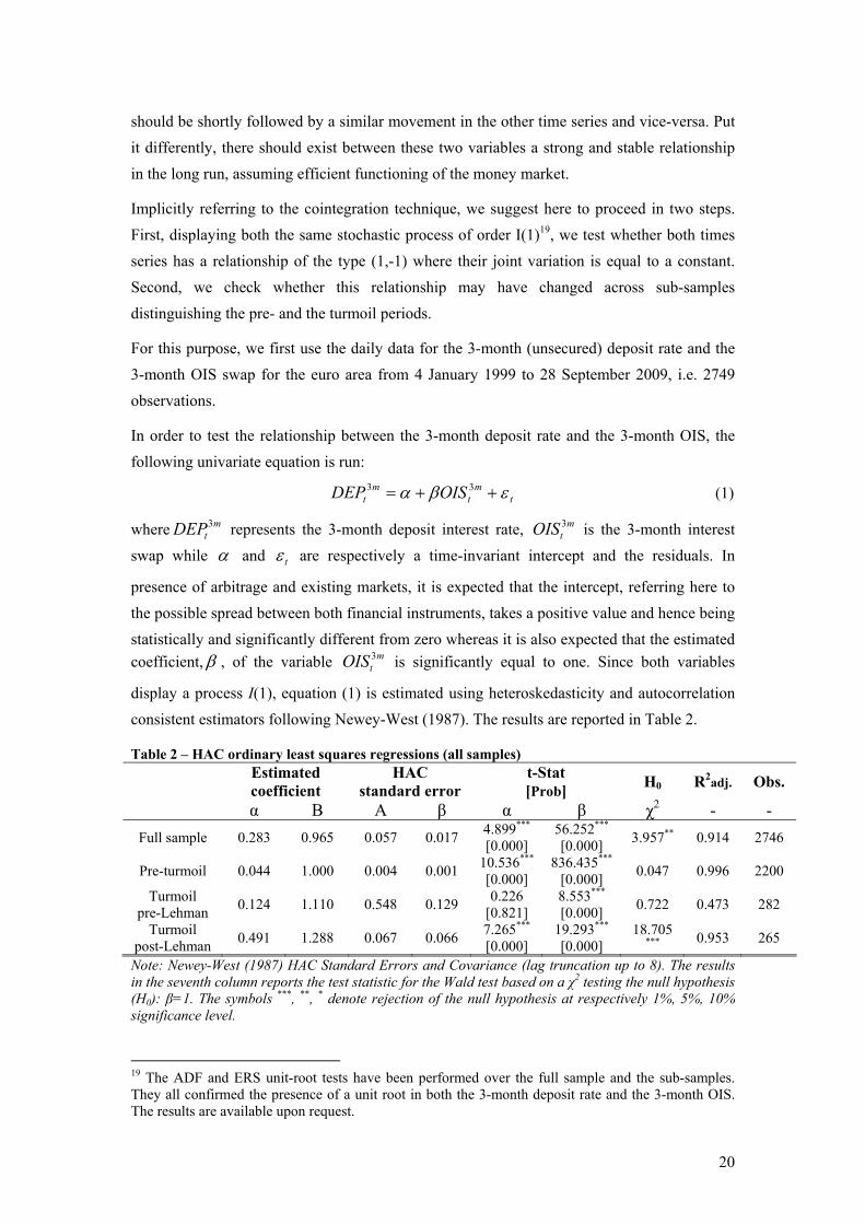
display a process I(1), equation (1) is estimated using heteroskedasticity and autocorrelation consistent estimators following Newey-West (1987). The results are reported in Table 2.

Table 2 – HAC ordinary least squares regressions (all samples)

Estimated coefficient

HAC standard error

t-Stat [Prob] H0 R2adj. Obs.

α Β Α β α β χ2 - - Full sample 0.283 0.965 0.057 0.017 4.899***

[0.000] 56.252*** [0.000] 3.957** 0.914 2746

Pre-turmoil 0.044 1.000 0.004 0.001 10.536*** [0.000]

836.435*** [0.000] 0.047 0.996 2200

Turmoil pre-Lehman 0.124 1.110 0.548 0.129 0.226

[0.821] 8.553*** [0.000] 0.722 0.473 282

Turmoil post-Lehman 0.491 1.288 0.067 0.066 7.265***

[0.000] 19.293*** [0.000]

18.705 *** 0.953 265

Note: Newey-West (1987) HAC Standard Errors and Covariance (lag truncation up to 8). The results in the seventh column reports the test statistic for the Wald test based on a χ2 testing the null hypothesis (H0): β=1. The symbols ***, **, * denote rejection of the null hypothesis at respectively 1%, 5%, 10% significance level.

19 The ADF and ERS unit-root tests have been performed over the full sample and the sub-samples. They all confirmed the presence of a unit root in both the 3-month deposit rate and the 3-month OIS. The results are available upon request.

21

For the full sample covering the period from 4 January 1999 to 28 September 2009, the null hypothesis of 1=β is strongly rejected whereas the intercept α is significantly different

from zero. In light of this result, it appears relevant to look then at the dynamics of equation (1) across sub-samples, insulating the pre-turmoil period (i.e. from 4 January 1999 to 8 August 2007) from the turmoil one. For the turmoil period starting on 9 August 2007, two sub-samples are also defined: (1) the turmoil period prior to the collapse of Lehman Brothers, i.e. the so-called pre-Lehman from 9 August 2007 to 12 September 2008; and (2) the turmoil period since the collapse of Lehman Brothers, i.e. the so-called post Lehman from 15 September 2008 to 28 September 2009.

Not surprisingly, in the pre-turmoil sample, the parameters of equation (1) display the expected values. The spread between the 3-month deposit rate and the 3-month OIS, given in Table 1 by the valueα , is significantly different from zero and positive, amounting 4.4 basis

points on average over this sample. In the same vein, the null hypothesis according to which the parameter β is significantly equal to 1 cannot be rejected. In addition, this estimation

displays a very good fit as the adjusted R2 is close to 1.

By contrast, the estimation results deteriorate substantially for the two sub-samples covering the turmoil period. For the pre-Lehman sample, although the null hypothesis 1=β cannot be

rejected, the value of the spread does not appear significantly different from zero. Moreover, the fit of the estimation decreases dramatically to 47% of explanatory power with respect to the data. Similarly, the results for the post-Lehman sample are mixed. While the explanatory power of equation (1) increases to 95% over this period, the null hypothesis that the parameter β is significantly equal to 1 is strongly rejected. However, the spread, which rises

to 49 basis points, appears significantly different from zero.

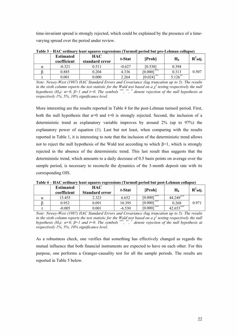
In sum, for the turmoil sample, equation (1) appears insufficient to explain the dynamics between both financial instruments. Put it simply, it could be argued accordingly that an omitted variable has gained in importance during the turmoil period whereas insignificant before the turmoil. In order to investigate this intuition, equation (1) is modified for the turmoil sample by including a deterministic trend. While adding a deterministic trend seems somewhat a-theoretical in this particular context, the purpose of this exercise is to check whether a regular pattern in the fluctuations of the deposit rate may be found. If yes, this could be the sign of a convergence among the quotes of market participants as regards their direction independently of the fluctuations of the OIS. The results are reported in Tables 3 and 4.

For the first sub-sample of the turmoil period, i.e. the pre-Lehman phase, the inclusion of the deterministic trend increases somewhat the explanatory power20 of equation (1) while this trend appears significantly different zero at 5% significance. By contrast, the existence of a 20 The adjusted R2 increases by 3.4% up to 50.7% instead of 47.3%.

22

time-invariant spread is strongly rejected, which could be explained by the presence of a time-varying spread over the period under review.

Table 3 – HAC ordinary least squares regressions (Turmoil period but pre-Lehman collapse)

Estimated coefficient

HAC standard error

t-Stat [Prob] H0 R2adj.

α -0.321 0.511 -0.627 [0.530] 0.394 β 0.885 0.204 4.336 [0.000] *** 0.313 t 0.001 0.000 2.264 [0.024] ** 5.126**

0.507

Note: Newey-West (1987) HAC Standard Errors and Covariance (lag truncation up to 5). The results in the sixth column reports the test statistic for the Wald test based on a χ2 testing respectively the null hypothesis (H0): α=0, β=1 and t=0. The symbols ***, **, * denote rejection of the null hypothesis at respectively 1%, 5%, 10% significance level.

More interesting are the results reported in Table 4 for the post-Lehman turmoil period. First, both the null hypothesis that α=0 and t=0 is strongly rejected. Second, the inclusion of a deterministic trend as explanatory variable improves by around 2% (up to 97%) the explanatory power of equation (1). Last but not least, when comparing with the results reported in Table 1, it is interesting to note that the inclusion of the deterministic trend allows not to reject the null hypothesis of the Wald test according to which β=1, which is strongly rejected in the absence of the deterministic trend. This last result thus suggests that the deterministic trend, which amounts to a daily decrease of 0.5 basis points on average over the sample period, is necessary to reconcile the dynamics of the 3-month deposit rate with its corresponding OIS.

Table 4 – HAC ordinary least squares regressions (Turmoil period but post-Lehman collapse)

Estimated coefficient

HAC Standard error

t-Stat [Prob] H0 R2adj.

α 15.455 2.323 6.652 [0.000] *** 44.249*** β 0.952 0.091 10.395 [0.000] *** 0.268 t -0.005 0.001 -6.530 [0.000] *** 42.653***

0.971

Note: Newey-West (1987) HAC Standard Errors and Covariance (lag truncation up to 5). The results in the sixth column reports the test statistic for the Wald test based on a χ2 testing respectively the null hypothesis (H0): α=0, β=1 and t=0. The symbols ***, **, * denote rejection of the null hypothesis at respectively 1%, 5%, 10% significance level.

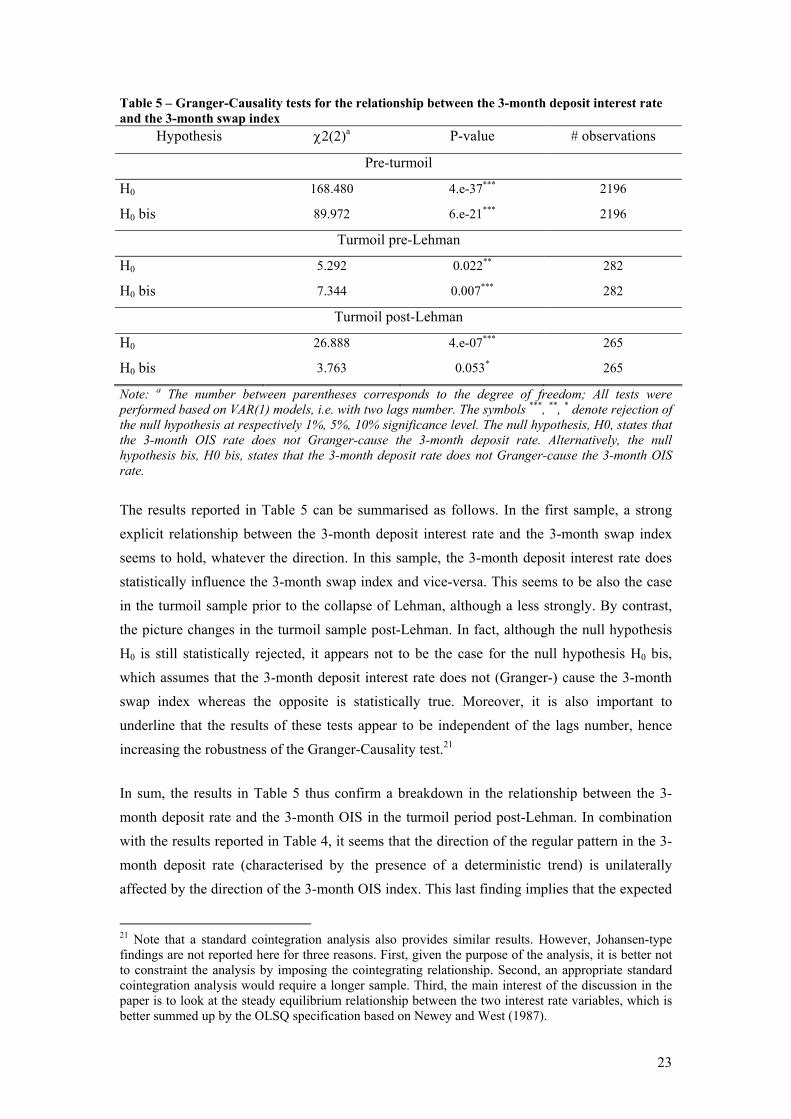
As a robustness check, one verifies that something has effectively changed as regards the mutual influence that both financial instruments are expected to have on each other. For this purpose, one performs a Granger-causality test for all the sample periods. The results are reported in Table 5 below.

23

Table 5 – Granger-Causality tests for the relationship between the 3-month deposit interest rate and the 3-month swap index

Hypothesis χ2(2)a P-value # observations

Pre-turmoil

H0 168.480 4.e-37*** 2196

H0 bis 89.972 6.e-21*** 2196

Turmoil pre-Lehman

H0 5.292 0.022** 282

H0 bis 7.344 0.007*** 282

Turmoil post-Lehman

H0 26.888 4.e-07*** 265

H0 bis 3.763 0.053* 265

Note: a The number between parentheses corresponds to the degree of freedom; All tests were performed based on VAR(1) models, i.e. with two lags number. The symbols ***, **, * denote rejection of the null hypothesis at respectively 1%, 5%, 10% significance level. The null hypothesis, H0, states that the 3-month OIS rate does not Granger-cause the 3-month deposit rate. Alternatively, the null hypothesis bis, H0 bis, states that the 3-month deposit rate does not Granger-cause the 3-month OIS rate.

The results reported in Table 5 can be summarised as follows. In the first sample, a strong explicit relationship between the 3-month deposit interest rate and the 3-month swap index seems to hold, whatever the direction. In this sample, the 3-month deposit interest rate does statistically influence the 3-month swap index and vice-versa. This seems to be also the case in the turmoil sample prior to the collapse of Lehman, although a less strongly. By contrast, the picture changes in the turmoil sample post-Lehman. In fact, although the null hypothesis H0 is still statistically rejected, it appears not to be the case for the null hypothesis H0 bis, which assumes that the 3-month deposit interest rate does not (Granger-) cause the 3-month swap index whereas the opposite is statistically true. Moreover, it is also important to underline that the results of these tests appear to be independent of the lags number, hence increasing the robustness of the Granger-Causality test.21

In sum, the results in Table 5 thus confirm a breakdown in the relationship between the 3-month deposit rate and the 3-month OIS in the turmoil period post-Lehman. In combination with the results reported in Table 4, it seems that the direction of the regular pattern in the 3-month deposit rate (characterised by the presence of a deterministic trend) is unilaterally affected by the direction of the 3-month OIS index. This last finding implies that the expected

21 Note that a standard cointegration analysis also provides similar results. However, Johansen-type findings are not reported here for three reasons. First, given the purpose of the analysis, it is better not to constraint the analysis by imposing the cointegrating relationship. Second, an appropriate standard cointegration analysis would require a longer sample. Third, the main interest of the discussion in the paper is to look at the steady equilibrium relationship between the two interest rate variables, which is better summed up by the OLSQ specification based on Newey and West (1987).

24

arbitrage between both segments of the money market is not working during the turmoil period.

5.2. Statistical evidence

In order to perform a robustness check of the previous findings, it appears interesting to check whether the apparent disconnection between the unsecured and the secured segments of the euro area money market (when using the quotes) is also reflected in the corresponding fixings. Indeed, in the early stage of the crisis, some have argued that the fixings for the unsecured segments were note correctly reflecting the developments of the corresponding quotes (i.e. the deposit rates). Against this background, it appears appropriate to analyse also the relationship between the EURIBOR and EONIA fixings both at the 3-month horizon. Nevertheless, given that the EONIA fixings are only recently available, this robustness check is confined to a statistical analysis over a shorter sample period, i.e. from 15 June 2007 to 13 July 2009.

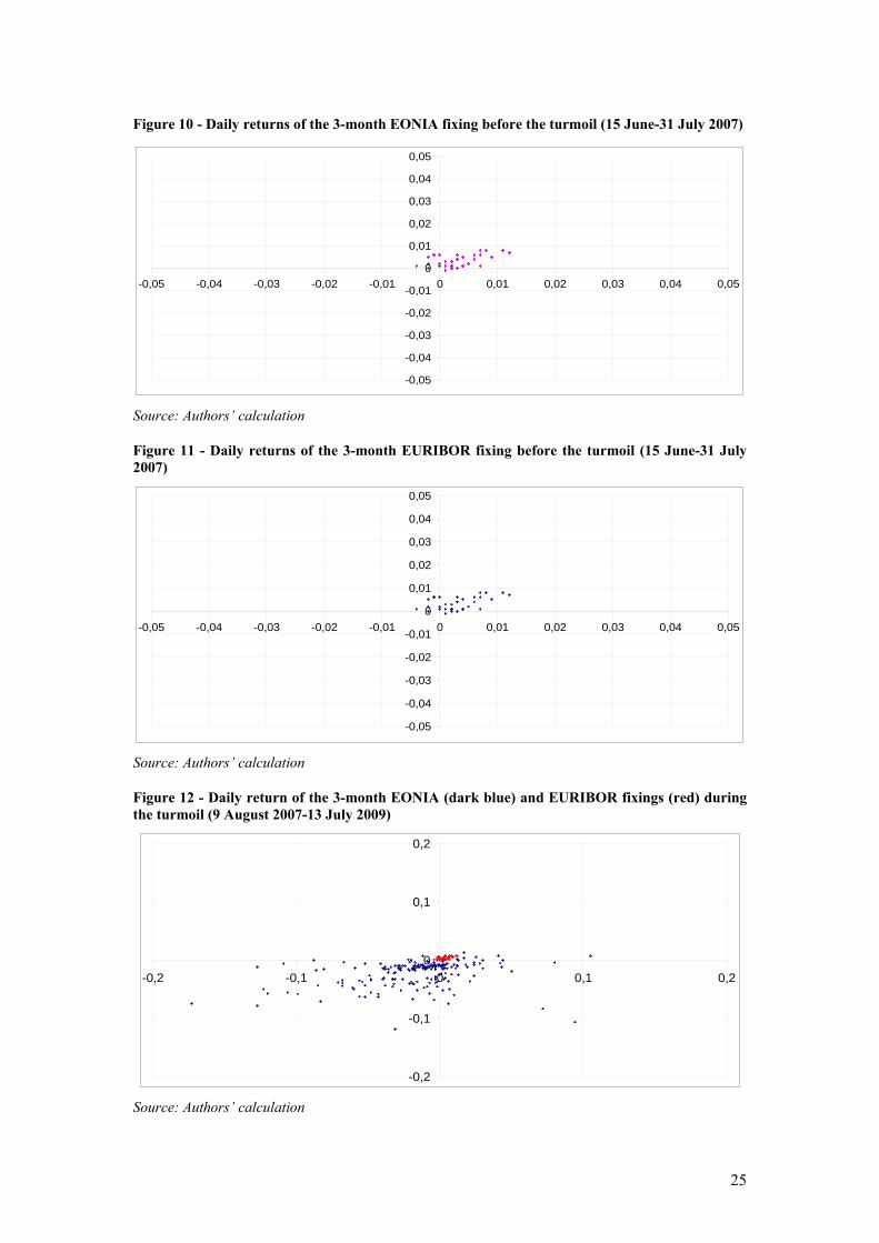
As shown by Figures 10-12 below, the empirical distribution of daily returns of the EONIA fixing matches very closely the empirical distribution the EURIBOR fixing, albeit same values, in the pre-turmoil period, i.e. from 15 June to 31 July 2007. By contrast, in the turmoil period, i.e. from 9 August 2007 to 13 July 2009, a substantial modification of the pattern of each fixing is observed. In particular, the 3-month EURIBOR fixing displays a lower dispersion than the 3-month EONIA fixing.

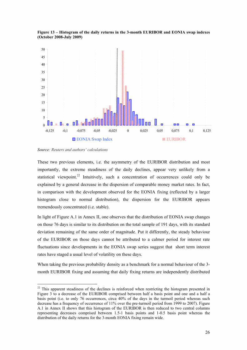
When looking at the turmoil period post-Lehman, similar evidence is observed. Over the period ranging from the 10 October 2008 to the 13 July 2009, which includes 191 Target days, the 3-month EONIA swap index increased 56 times (29% of the days) and decreased 133 times (70% of the days). At the same time, the 3-month EURIBOR increased 16 times (8% of the days) and decreased 169 times (88% of the days). Furthermore the decrease was between half a basis point and one and a half a basis point in 76 occurrences, i.e. 40% of the days. Another way to present this concentration of quotes for the EURIBOR under the crisis period is to plot the histogram of the occurrences for both fixings. Figure 13 below shows the histogram of the daily increases of both the 3-month EONIA swap index and the 3-month EURIBOR during those 191 TARGET days.

25

Figure 10 - Daily returns of the 3-month EONIA fixing before the turmoil (15 June-31 July 2007)

-0,05

-0,04

-0,03

-0,02

-0,01

0

0,01

0,02

0,03

0,04

0,05

-0,05 -0,04 -0,03 -0,02 -0,01 0 0,01 0,02 0,03 0,04 0,05

Source: Authors’ calculation

Figure 11 - Daily returns of the 3-month EURIBOR fixing before the turmoil (15 June-31 July 2007)

-0,05

-0,04

-0,03

-0,02

-0,01

0

0,01

0,02

0,03

0,04

0,05

-0,05 -0,04 -0,03 -0,02 -0,01 0 0,01 0,02 0,03 0,04 0,05

Source: Authors’ calculation

Figure 12 - Daily return of the 3-month EONIA (dark blue) and EURIBOR fixings (red) during the turmoil (9 August 2007-13 July 2009)

-0,2

-0,1

0

0,1

0,2

-0,2 -0,1 0 0,1 0,2

Source: Authors’ calculation

26

Figure 13 – Histogram of the daily returns in the 3-month EURIBOR and EONIA swap indexes (October 2008-July 2009)

0

5

10

15

20

25

30

35

40

45

50

-0,125 -0,1 -0,075 -0,05 -0,025 0 0,025 0,05 0,075 0,1 0,125

EONIA Swap Index EURIBOR

Source: Reuters and authors’ calculations

These two previous elements, i.e. the asymmetry of the EURIBOR distribution and most importantly, the extreme steadiness of the daily declines, appear very unlikely from a statistical viewpoint.22 Intuitively, such a concentration of occurrences could only be explained by a general decrease in the dispersion of comparable money market rates. In fact, in comparison with the development observed for the EONIA fixing (reflected by a larger histogram close to normal distribution), the dispersion for the EURIBOR appears tremendously concentrated (i.e. stable).

In light of Figure A.1 in Annex II, one observes that the distribution of EONIA swap changes on those 76 days is similar to its distribution on the total sample of 191 days, with its standard deviation remaining of the same order of magnitude. Put it differently, the steady behaviour of the EURIBOR on those days cannot be attributed to a calmer period for interest rate fluctuations since developments in the EONIA swap series suggest that short term interest rates have staged a usual level of volatility on these days.

When taking the previous probability density as a benchmark for a normal behaviour of the 3-month EURIBOR fixing and assuming that daily fixing returns are independently distributed

22 This apparent steadiness of the declines is reinforced when restricting the histogram presented in Figure 3 to a decrease of the EURIBOR comprised between half a basis point and one and a half a basis point (i.e. to only 76 occurrences, circa 40% of the days in the turmoil period whereas such decrease has a frequency of occurrence of 11% over the pre-turmoil period from 1999 to 2007). Figure A.1 in Annex II shows that this histogram of the EURIBOR is then reduced to two central columns representing decreases comprised between 1.5-1 basis points and 1-0.5 basis point whereas the distribution of the daily returns for the 3-month EONIA fixing remain wide.

27

and follow a discrete binomial process, a probability based on a binomial distribution process can be calculated as follows (by using n for the number of consecutive trials, p for the probability of a positive outcome, and k the number of positive outcome):

knkknpn ppCkprob −−⋅⋅= )1()(,

Let us now consider the case of 191 consecutive trials yielding 76 times an outcome having an 11% probability of occurrence. In this case:

( )25

7619176

761917676191

10.7

)89.0()11.0(!76191!76

!191)89.0()11.0(

−

−

−

=

⋅⋅−

=

⋅= Cprob

The previous probability thus suggests that the probability of such depreciation outcome over a very short period of time, based on the pre-turmoil statistical properties of the EURIBOR fixing time series, is pretty low, that is close to zero. This statistical finding thus confirms the econometric results for the deposit and swap rates, both suggesting that the EURBOR fixing rates have followed over the recent turmoil period an extremely unusual steady downward pace (i.e. a deterministic pace rather than the usually “stochastic” diffusion process), irrespectively of the average volatility observed on neighbouring market segment.

The previous findings may imply, among other things, that the fixing could be the result of converging pricing among prime banks not entirely reflecting market conditions, hence making the fixing entirely virtual. By nature, if it is so for the EURIBOR, then it is quite likely that the USD and GBP counterpart, which are the 3-month LIBOR, also have a somewhat virtual nature. In the same vein, if the fixings of 3-month interest rates appear artificial, there is no compelling reason why this should not also be the case for the fixing of longer maturities and in particular for the 1-year fixings, clearly putting at risk the anchoring role of these fixings in the financial markets.

Finally, one may wonder whether such “virtual pricing” of the EURIBOR may result mainly from euro area continental banks in the EBF panel or whether it also applies to non euro area international banks. To answer that question, a synthetic LIBOR index for EUR(named LiborUK-LIBOR) is calculated on the basis of the various contributions which only includes BBA’s panel banks which do not contribute to the EURIBOR fixing made by EBF. Figure 14 below reports the comparison of this synthetic index with both the LIBOR fixing for the EUR segment and the EURIBOR, both for the 3-month maturity. Interestingly, it can be noted that the dispersion of the pricing made between by international (mostly London-based) banks with respect to the pricing made by euro area banks in the EURIBOR panel has increased significantly since the beginning of 2009. When combining this information with the previous

28

statistical evidence, it appears that the regular daily decrease of between 0.5 and 1.5 basis points seems to mostly reflect a “convergence of views” within the euro area banks.

Figure 14 – Spread between the 3-month fixing for a synthetic EUR LIBOR and the LIBOR/EURIBOR rates in EUR

-0.06

-0.04

-0.02

0

0.02

0.04

0.06

09/1

0/08

23/1

0/08

06/1

1/08

20/1

1/08

04/1

2/08

18/1

2/08

01/0

1/09

15/0

1/09

29/0

1/09

12/0

2/09

26/0

2/09

12/0

3/09

26/0

3/09

09/0

4/09

23/0

4/09

07/0

5/09

21/0

5/09

04/0

6/09

18/0

6/09

02/0

7/09

16/0

7/09

30/0

7/09

Spread LiborUK-LIBORSpread LiborUK-EURIBOR

Source: Reuters and authors’ calculations

6. Concluding remarks

In this paper, we have started by outlining how secular developments in commercial banks’ funding practices and the move towards financial disintermediation have resulted in deep-rooted changes to the functioning of money markets. Hence, these developments have consequently affected the information content and significance of traditional money market fixings. After reviewing the nature of the arbitrage relationships existing between money market derivative prices and the related underlying cash segments, we have tried to analyse how these pricing parities have held up during the turmoil (or not). Using different numerical techniques (univariate, multivariate and probabilistic), we have tried to highlight the dynamics of money market fixings, and of the related derivative prices during the turmoil, by slicing the crisis into three sub-periods (pre-turmoil (i.e. before August 2007), turmoil until Lehman’s demise, and post Lehman, i.e. after September 2008).

The findings reported in the paper suggest that, in the pre-turmoil period (i.e. prior to August 2007) both deposit rates and their derivative equivalent were linked by a very strong relationship, with two-way sided interactions reflecting the strength of arbitrage. By contrast, the onset of the turmoil brought about a weakening of this relationship on the account of a gradual dis-anchoring of deposit rates with respect to the OIS. Although the explanatory power of the simple model proposed in this paper increases in the post-Lehman period,

29

Granger-causality tests suggest that the direction of deposit rates and fixings were set univocally by the OIS, while an omitted variable seem to have gotten into get into play. In particular, it appears that the addition of a deterministic trend into the regression model during the post-Lehman period helps find again the co-movement expected these two financial instruments. Put it simply, the added deterministic trend support both the re-connection of the two series and the one-way sided nature of their relationship post-Lehman. Finally, a probability-based analysis using a binomial law supports the former finding that something “deeply unusual” happened on Euribor fixings post-Lehman. The economic meaning of such deterministic trend is not easy as it could reflect various phenomena, epitomizing for instance a hypothetical coordination between individual fixing contributors.

These findings raise some questions. Although the issue of the quality and the accuracy of money market fixings may be deemed not central for monetary policy-making, it might affect the transmission channels of monetary policy, if prolonged over an extended period of time. Indeed, given the anchoring role played unsecured segment fixings in the money and capital markets (including retail banks’ interest rates to the economy), the risk of opportunistic behaviour tainting the production of market references should be avoided. Likewise, the issues related to the lack of depth of the unsecured money market on the term, and of the related consequences in terms of accuracy of the fixings, should also be addressed.

Practically a discussion on the production of fixings rates should aim at overcoming the following issues. First, fixing procedures should reflect better commercial banks’ liability mix and the growing role of NBFIs, and overcome the outdated “peer-to-peer” approach that inspired fixing procedures at their inception. Second the governance of fixings should be more active, and involve frequent due diligence to avoid opportunistic behaviours and other dis-anchoring. This may lead in practice to a broadening of the financing base underlying fixings by including CDs, tripartite repos operations on non-government collateral (down to investment grade), and any other funding operations that represent a de facto proxy of an unsecured funding operation.

Another challenge could be to revive the unsecured money market through a less asymmetric supervisory framework. Indeed the crisis has shown that a too tight regulatory capital approach towards unsecured operations seem to have generated an adverse selection phenomenon. High regulatory capital charges have forcefully pushed banks towards the repo market, where large pockets of under priced risk have developed, while at the same time hollowing out the liquidity of the traditional money market beyond one month. The demise of the non-government segment of the repo market following the collapse of Lehman Brothers has generated a liquidity panic that the traditional segment of the money market was unable to withstand alone, hence requiring unprecedented interventions of central banks around the world.

30

7. References

Bank of England, 2007. An indicative decomposition of Libor spreads. Quarterly Bulletin, fourth quarter, pp. 498–99.

Bank of England, 2009. Pricing anomalies in financial markets. Quarterly Bulletin, first quarter, pp. 498–99.

Belton, T., Roever, A., Bassi, F., Ramaswamy, S., 2008. The outlook for Libor. JP Morgan Note on the US Fixed Income Strategy, 16 May.

Borgy, J.F., 2007. Can financial markets rely any more on 3 and 6 month Libor or Euribor fixings? Natixis Flash, 19 November.

Chadha, J.S., Durré, A., 2009. Pathology of a Heart Attack: the interbank lending market. University of Kent, mimeo.

Christensen, J.H.E., Lopez, J.A., Rudebusch, G.D., 2009. Do central bank liquidity facilities affect interbank lending rates? Federal Reserve Bank of San Francisco, mimeo.

European Central Bank, 2008. Money Market Study 2008.

European Central Bank, 2009. Money Market Survey. September.

Ewerhart, C., Cassola, N., Ejerskov, S., Valla, N., 2007. Manipulation in money markets. International Journal of Central Banking, March, pp. 113–48.

Financial Times, 2009. Fall in Libor fails to paint a true picture. June 4.

Gyntelberg, J, Wooldridge, P., 2008. Interbank rate fixings during the recent turmoil. Bank for International Settlements Quarterly Review, March.

International Monetary Fund, 2008. Global Financial Stability Report. Spring.

Keister, T., McAndrews, J., 2009. Why are banks holding so many excess reserves? Federal Reserve Bank of New York Staff Reports, No. 380.

Lehman Brothers, 2008. Libor “misquoting”: A possible explanation. European Interest Rate Strategies, April 18.

MacKenzie, D., 2008. What’s in a number? The importance of LIBOR. University of Edinburgh, Real-World Economics Review, No. 47.

31

Michaud, F.L., Upper, C., 2008. What drives interbank rates? Evidence from the Libor panel. Bank for International Settlements Quarterly Review, March.

Taylor, J.B., Williams, J.C., 2008. A black swan in the money market. Federal Reserve Bank of San Francisco Working Paper Series, 2008-04.

32

ANNEX I

Definition and composition of the LIBOR/EURIBOR

The unsecured interest rates used in the note are of two types. On the one hand, unsecured interest rates are presented on the basis of the LIBOR. On the other hand, the EURIBOR interest rates are used. The purpose of both types is similar, only the panel of surveyed banks differs.

Strictly, the LIBOR is defined as: “The rate at which an individual Contributor Panel bank

could borrow funds (i.e. unsecured interbank cash or cash raised through primary issuance of interbank Certificates of Deposit), were it to do so by asking for and then accepting inter-bank offers in reasonable market size, just prior to 11.00 London time.” In practice, this is the rate at which each bank submits must be formed from that bank’s perception of its cost of funds in the interbank market. In addition, it is specified that contributions must represent rates formed in London and not elsewhere and for the currency concerned. They should not be the cost of producing one currency by borrowing in another currency and accessing the required currency via the foreign exchange markets. The rates must be submitted by members of staff at a bank with primary responsibility for management of a bank’s cash, rather than a bank’s derivative book.

On the British Bankers' Association (BBA) website23, it is also recalled that the key concept is that LIBOR is based upon the offered rate, and not the bid rate. Every contributor bank is asked to base their bbalibor submissions on the following question; “At what rate could you borrow funds, were you to do so by asking for and then accepting inter-bank offers in a reasonable market size just prior to 11 am?” Therefore, submissions are based upon the lowest perceived rate that a bank on a certain currency panel could go into the inter-bank money market and obtain sizable funding, for a given maturity.

The rates are not based on actual transaction, indeed it would not be possible to create the suite of bbalibor rates if this was a requirement, as not all banks will require funds in marketable size each day in each of the currencies and maturities they quote. However, this does not mean the rates do not reflect true cost of interbank funding. A bank will know what its credit and liquidity risk profile is from rates at which it has dealt, and can construct a curve to predict accurately the correct rate for currencies or maturities in which it has not been active.

“Reasonable market size” is intentionally left loosely defined. This is because it would have to be constantly monitored, and in the current conditions it would have to be changed almost 23 http://www.bba.org.uk/bba/jsp/polopoly.jsp?d=141&a=15881.

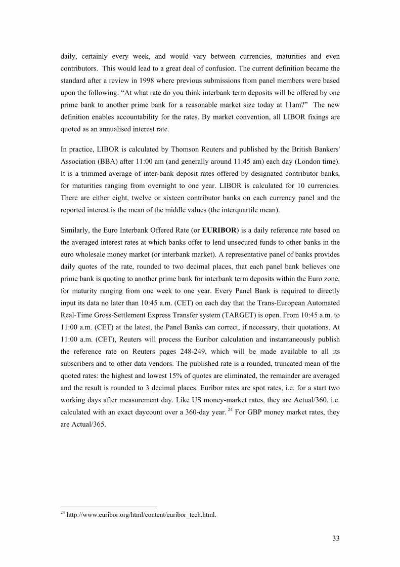
33

daily, certainly every week, and would vary between currencies, maturities and even contributors. This would lead to a great deal of confusion. The current definition became the standard after a review in 1998 where previous submissions from panel members were based upon the following: “At what rate do you think interbank term deposits will be offered by one prime bank to another prime bank for a reasonable market size today at 11am?” The new definition enables accountability for the rates. By market convention, all LIBOR fixings are quoted as an annualised interest rate.

In practice, LIBOR is calculated by Thomson Reuters and published by the British Bankers' Association (BBA) after 11:00 am (and generally around 11:45 am) each day (London time). It is a trimmed average of inter-bank deposit rates offered by designated contributor banks, for maturities ranging from overnight to one year. LIBOR is calculated for 10 currencies. There are either eight, twelve or sixteen contributor banks on each currency panel and the reported interest is the mean of the middle values (the interquartile mean).

Similarly, the Euro Interbank Offered Rate (or EURIBOR) is a daily reference rate based on the averaged interest rates at which banks offer to lend unsecured funds to other banks in the euro wholesale money market (or interbank market). A representative panel of banks provides daily quotes of the rate, rounded to two decimal places, that each panel bank believes one prime bank is quoting to another prime bank for interbank term deposits within the Euro zone, for maturity ranging from one week to one year. Every Panel Bank is required to directly input its data no later than 10:45 a.m. (CET) on each day that the Trans-European Automated Real-Time Gross-Settlement Express Transfer system (TARGET) is open. From 10:45 a.m. to 11:00 a.m. (CET) at the latest, the Panel Banks can correct, if necessary, their quotations. At 11:00 a.m. (CET), Reuters will process the Euribor calculation and instantaneously publish the reference rate on Reuters pages 248-249, which will be made available to all its subscribers and to other data vendors. The published rate is a rounded, truncated mean of the quoted rates: the highest and lowest 15% of quotes are eliminated, the remainder are averaged and the result is rounded to 3 decimal places. Euribor rates are spot rates, i.e. for a start two working days after measurement day. Like US money-market rates, they are Actual/360, i.e. calculated with an exact daycount over a 360-day year. 24 For GBP money market rates, they are Actual/365.

24 http://www.euribor.org/html/content/euribor_tech.html.

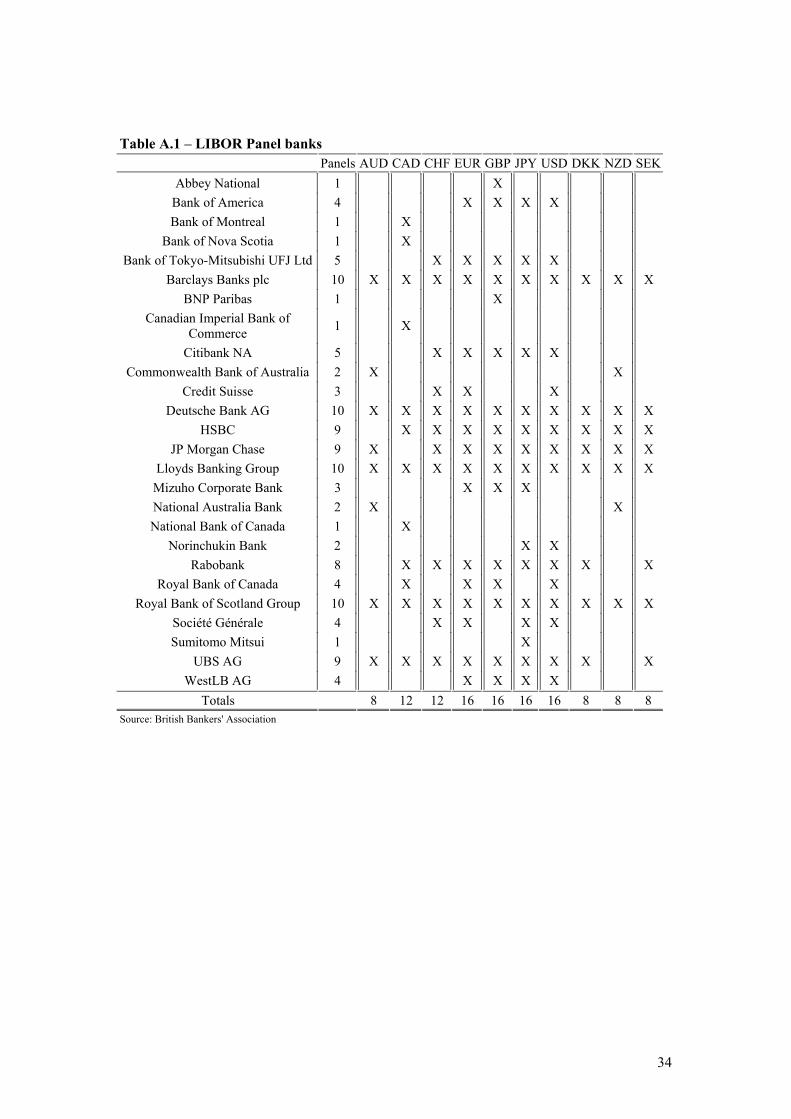
34

Table A.1 – LIBOR Panel banks Panels AUD CAD CHF EUR GBP JPY USD DKK NZD SEK

Abbey National 1 X Bank of America 4 X X X X Bank of Montreal 1 X

Bank of Nova Scotia 1 X Bank of Tokyo-Mitsubishi UFJ Ltd 5 X X X X X

Barclays Banks plc 10 X X X X X X X X X X BNP Paribas 1 X

Canadian Imperial Bank of Commerce 1 X

Citibank NA 5 X X X X X Commonwealth Bank of Australia 2 X X

Credit Suisse 3 X X X Deutsche Bank AG 10 X X X X X X X X X X

HSBC 9 X X X X X X X X X JP Morgan Chase 9 X X X X X X X X X

Lloyds Banking Group 10 X X X X X X X X X X Mizuho Corporate Bank 3 X X X National Australia Bank 2 X X National Bank of Canada 1 X

Norinchukin Bank 2 X X Rabobank 8 X X X X X X X X

Royal Bank of Canada 4 X X X X Royal Bank of Scotland Group 10 X X X X X X X X X X

Société Générale 4 X X X X Sumitomo Mitsui 1 X

UBS AG 9 X X X X X X X X X WestLB AG 4 X X X X

Totals 8 12 12 16 16 16 16 8 8 8 Source: British Bankers' Association

35

Table A.2 – EURIBOR Panel banks Countries Name

Austria Erste Bank der Österreichischen Sparkassen RZB - Raiffeisen Zentralbank Österreich AG

Belgium

Dexia Bank Fortis Bank KBC

Finland Nordea

France

BNP - Paribas Natixis Société Générale

Crédit Agricole s.a. HSBC France Crédit Industriel et Commercial CIC

Germany

Landesbank Berlin WestLB AG Bayerische Landesbank Girozentrale Commerzbank Deutsche Bank DZ Bank Deutsche Genossenschaftsbank

Dresdner Bank Landesbank Baden-Württemberg Girozentrale Landesbank Hessen - Thüringen Girozentrale Norddeutsche Landesbank Girozentrale

Greece National Bank of Greece

Ireland AIB Group Bank of Ireland

Italy

Banca IntesaBci UCI Milan Monte dei Paschi di Siena

Luxembourg Banque et Caisse d'Épargne de l'État

Netherlands

ABN Amro Bank Rabobank ING Bank

Portugal Caixa Geral De Depósitos (CGD)

Spain

Banco Bilbao Vizcaya Argentaria Confederacion Española de Cajas de Ahorros Banco Santander Central Hispano

Other EU Banks

Barclays Capital Den Danske Bank Svenska Handelsbanken

International Banks

Bank of Tokyo - Mitsubishi J.P. Morgan Chase & Co.

Citibank UBS (Luxembourg) S.A.

Source: European Banking Federation and Financial Markets Association

36

ANNEX II

Figure A.1 – Histogram of the daily returns of 3-month EURIBOR and EONIA fixings restricted to the 76 days where the EURIBOR changes were comprised between -1.5 and -0.5 basis point (10 October 2008-13 July 2009)

0

5

10

15

20

25

30

35

40

45

50

-0,125 -0,1 -0,075 -0,05 -0,025 0 0,025 0,05 0,075 0,1 0,125

EONIA Swap Index EURIBOR

Source: Reuters and authors’ calculations