INTERACTIVE THIN SHELLS – AN INTERFACE FOR

THE ANALYSIS OF PHYSICALLY BASED ANIMATION

A Thesis

Presented to

the Faculty of California Polytechnic State University San Luis Obispo

In Partial Fulfillment

of the Requirements for the Degree

Master of Science in Computer Science

by

James Ross Skorupski

September 2006

ii

AUTHORIZATION FOR REPRODUCTION OF MASTER’S

THESIS

I reserve the reproduction rights of this thesis for a period of five years from the date of

submission. I waive all reproduction rights after that time span has expired.

_________________________________________________________ Signature _________________________________________________________ Date

iii

APPROVAL PAGE

TITLE: Interactive Thin Shells – An Interface for the Analysis of Physically Based

Animation

AUTHOR: James Ross Skorupski

DATE SUBMITTED: September 2006

Dr. Zoë Wood ____________________________________ Advisor or Committee Chair Signature Dr. Mei-Ling Liu ____________________________________ Committee Member Signature Dr. Franz Kurfess ____________________________________ Committee Member Signature

iv

Abstract

Interactive Thin Shells – An Interface for the Analysis of Physically Based

Animation James Ross Skorupski

With the advent of real-time physically based animation over the past decade, and

more recently, the growth of general mathematical computing on graphics processors, there has been an increasing interest in the development of realism in computer graphics. However, the algorithms involved in mimicking the physical world are often very complex, abstract, and out of reach for an average computer science student or practitioner. This work introduces an interface to a physically based algorithm, a thin shell animation, which focuses on visualization, experimentation, and control. Through the use of dynamic coloring, abstract visual cues, robust user interaction, and full control over the algorithm parameters, our system facilitates the process of discovery and experimentation, which can enhance the learning experience and help overcome the difficulties in understanding the mathematically intense concepts that comprise the core of many physically based models. Furthermore, our interface design can be used as model for interacting with other types of physically based animations and provide the same benefits for learning.

v

Table of Contents Table of Figures ................................................................................................................. vi 1 Problem Description and Motivation.......................................................................... 1

1.1 Contribution ........................................................................................................ 3 2 Related Work .............................................................................................................. 5 3 Solution Overview .................................................................................................... 10

3.1 Animation ......................................................................................................... 10 3.2 User Interaction................................................................................................. 11 3.3 Visualization ..................................................................................................... 12

3.3.1 Dynamic Histogram.................................................................................. 13 3.3.2 Animation Cache ...................................................................................... 15

4 Implementation ......................................................................................................... 17 4.1 Animation ......................................................................................................... 17

4.1.1 Implicit and Explicit Integration............................................................... 17 4.1.2 Forces and Constraints.............................................................................. 19 4.1.3 Boundaries and Object Collisions............................................................. 23 4.1.4 Adaptive Time Steps................................................................................. 24

4.2 User Interaction................................................................................................. 24 4.2.1 Live Interaction......................................................................................... 25 4.2.2 Paused Interaction..................................................................................... 26 4.2.3 Synchronized Interaction .......................................................................... 26

4.3 Visualization ..................................................................................................... 27 4.3.1 Histogram Compression............................................................................ 28 4.3.2 Histogram Equalization ............................................................................ 31 4.3.3 Animation Cache ...................................................................................... 33

4.4 Full Feature List................................................................................................ 33 5 Results....................................................................................................................... 36

5.1 User Interface Overview................................................................................... 36 5.2 Animation Features........................................................................................... 38 5.3 User Interaction................................................................................................. 40 5.4 Visualization ..................................................................................................... 42 5.5 Thin Shell Model Weaknesses.......................................................................... 44 5.6 Performance ...................................................................................................... 48

6 Conclusions............................................................................................................... 50 7 Future Work .............................................................................................................. 53 8 Bibliography ............................................................................................................. 55

vi

Table of Figures Figure 1 - A force value histogram, with corresponding hue value mappings ................. 15 Figure 2 - The explicit and implicit integration schemes used in ITS.............................. 19 Figure 3 – The ITS Animation Membrane and Bending Forces ...................................... 22 Figure 4 - The Linear Bending Force Weakness .............................................................. 23 Figure 5 - The ITS histogram compression algorithm...................................................... 31 Figure 6 - Histogram Equalization.................................................................................... 32 Figure 7 - The ITS Graphical User Interface .................................................................... 37 Figure 8 - ITS supports arbitrary mesh files. .................................................................... 38 Figure 9 - Two mesh experiments .................................................................................... 39 Figure 10 - ITS supports simple vertex collision with the environment........................... 40 Figure 11 - A simultaneous experiment with pinned v-beams. ........................................ 41 Figure 12 - Live Interaction .............................................................................................. 41 Figure 13 - Visible force vectors and vertex coloring ...................................................... 42 Figure 14 - The progression of forces in four experiments .............................................. 43 Figure 15 - Histogram Compression and Equalization..................................................... 46 Figure 17 - Unrealistic Forces........................................................................................... 48 Figure 18 - A comparison of VIS requirements and the ITS implementation.................. 50

1

1 Problem Description and Motivation

One of the many current driving goals in the field of computer graphics is to artificially

replicate reality by mimicking the appearance of natural objects and phenomena. While

the ultimate purpose of the resulting imagery may vary widely from entertainment to

scientific endeavor, the underlying algorithms that produce the imagery of interest are,

more often than not, based on our basic scientific understanding of the world around us,

and therefore mathematically intensive. These algorithms and their associated techniques,

which often deal with real world phenomena such as fluid dynamics, rigid body

dynamics, and the transport of light, are grouped into a subset of computer graphics

known as physically based modeling [1]. The complexity of these algorithms is often

proportional to the desired amount of realism and the level of mathematical knowledge

and experience required to understand and successfully implement these algorithms can

often exceed the capabilities of a typical computer science practitioner. Furthermore,

these programs ultimately can only discretely approximate the continuous nature of

reality, and are therefore guaranteed to introduce some level of error which must be

understood and dealt with appropriately.

While traditionally, modeling the physics of reality has been delegated to large clusters of

servers computing over the course of hours or days, the rapid advancement in processing

power and memory storage sizes over the past decade has allowed for relatively complex

physically based algorithms to perform at interactive frame rates [1], [2]. In addition, the

market for home computer and entertainment console gaming has increased dramatically,

2

and the quest for realism in computer graphics in general has been hastened by the quest

for realism in interactive entertainment. Modern graphics cards manufacturers, similarly

driven by the home entertainment market, are beginning to encourage the development of

general purpose mathematical computing algorithms specifically designed for the highly

parallel stream architecture of graphics processing units, while other hardware vendors

are developing dedicated solutions that attempt to accelerate the mathematical operations

common in physically based modeling [19], [25]. Together, these technological and

financial motivations to develop more realistic computer imagery will inevitably further

the interest in physically based modeling, and encourage computer scientists to explore

the concepts associated with the field.

As technology advances and more complex physically based algorithms continue to

develop and become a feasible avenue for generating computer imagery, the

understanding of these algorithms and their underlying concepts will become a greater

challenge. In addition, as the demand for realism in the virtual world spreads across all

areas of the real world, computer scientists wishing to design physically based algorithms

will encounter an increasingly varied amount of scientific theory, ranging from

thermodynamics to astrophysics. To make matters worse, previous research has shown

that many modern computer science students encounter a small selection of math courses

in their curriculum, and therefore tend to exhibit weak mathematical problem solving

skills [3], [12], [6]. It is also safe to assume that many modern computer scientists, who

are recent university graduates, may be similarly lacking in mathematical background

required to understand many of concepts in physically based models.

3

The problem therefore presents itself: How can computer scientists, students and

practitioners alike, better understand the workings of math-intensive computer graphics

algorithms without an extensive math background? Our solution cannot eliminate the

need for traditional study in the requisite mathematical topics. It does, however, present a

tool to augment the learning process, and provide a more interactive and visual

experience for a person wishing to understand the behaviors of these complex algorithms.

1.1 Contribution

This work introduces an interface to a physically based algorithm that focuses on

visualization, experimentation, and control, and encourages the exploration, discovery,

and understanding of the algorithm as a whole. Through the use of dynamic coloring,

abstract visual cues, mouse interaction, and full control over the algorithm parameters,

our system facilitates the process of experimentation, which can enhance the learning

experience and help overcome the difficulties in understanding the mathematically

intense concepts that underlie our specific algorithm. Furthermore, our interface design

can be used as model for interfacing with similar algorithms and provide the same

benefits for learning. Our system’s target audience includes computer science students

and computer science practitioners with a desire to understand the complex workings of a

physically based algorithm and augment their learning experience with direct, visual

interaction.

Our interface is specifically designed for interacting with algorithms in a subset of

physically based modeling, called physically based animation. This sub-field deals with

4

the physical dynamics of mass, ranging from fluids to cloth, and involves the calculation

of internal and external energies that influence the resulting physical movement of the

system. Physically based animation algorithms facilitate a more natural graphical

interface, because they mimic physical motion which can be observed and often

confirmed in the real world. Other physically based modeling algorithms, such as those

that deal with thermodynamics or lighting models, may not lend themselves well to our

specific interface, but the general design concepts behind our system may provide a

guideline for future work which involves interaction with those types of algorithms.

The program we created to demonstrate our interface is called Interactive Thin Shells

(ITS). The underlying physically based algorithm simulates the dynamics of thin shells,

which are flexible structures that have a high ratio of width to thickness and have an

initial three dimensional non-flat shape that affects its energetic reaction to change from

that initial shape [9]. Our implementation of the physical system is based on a simplified

constraint model based partially off of previous work of in the area of thin shells [9] and

mass-spring cloth simulation [4]. We also implemented both an implicit and explicit

integration scheme developed by additional work in the area of cloth dynamics [15], [16],

[20]. The ITS environment allows us to directly demonstrate how our interface can be

used to investigate the properties of an algorithm and interact with it in an intuitive and

reasonable manner. In addition, the freeform interactive design of our interface, as is

described in Sections 3 and 4, serves to reveal a weakness in our thin shell algorithm and

discrete approximations of continuous material properties as a whole.

5

2 Related Work

The Interactive Thin Shells environment aims to provide a highly customizable and

intuitive interactive interface to a physically based animation algorithm. It sets itself apart

as a tool for those not intimately involved in the implementation details of the underlying

physical simulation, and therefore must focus on allowing the user to explore and

discover the capabilities of the underlying algorithm. Because the ITS environment itself

involves both the implementation of a physical model of thin shells and its unique

interface to that same model, it is based on previous work in the areas of physically based

animation, cloth simulation, and visual interactive simulation tools.

The thin shell algorithm implementation in ITS is based on a standard physically based

animation model, described in detail in the work of Baraff and Witkin [1]. The ITS

environment involves the persistent storage of a series of states of the system,

advancement of the states using the forces of a chosen dynamics model, thin shells with

masses at each vertex in this case, and numerical integration of this progression which

results in movement in the simulation environment. More specifically, the underlying

model implementation is equivalent to a cloth animation model with some modifications

that support non-planar initial configurations and the stiffer internal forces of thin shell

materials.

The ITS system also employs implicit integration to progress the simulation, as described

Baraff and Witkin in their earlier development of stable, stiff cloth [2]. The backward

6

Euler step integration scheme is utilized for implicit integration, and the traditional

forward Euler step method is used for our explicit integration mode [1]. While it is a

more complicated scheme for calculating the next state of the thin shells model, which

requires the solving of a large linear system at each step of the simulation, the implicit

method provides for numerical stability that is critical in this particular situation [1]. Our

particular implementation of the implicit method is based on the work of Dean Marci of

the Intel Corporation [15]. Thin shell materials typically exhibit very little deformation

within the surface of the material itself, and therefore require high resistance to these

local changes in length in area. Because of this, our simulation will experience regions of

high energy in response to deformation, where implicit differentiation allows for

reasonably sized time steps [1].

Thin shells, as mentioned in Section 1.1, are flexible materials that are extremely thin in

one dimension and have a predetermined relaxed non-flat configuration [9]. They

typically are very resistant to in-plane deformation, in the form of stretching or shearing,

and allow a limited amount of out-of-plane bending from the original shape. Thin shell

materials differ themselves from cloth, which is typically modeled with an initial flat

configuration and weaker membrane and bending energies. The membrane, or in-plane

forces in our algorithm are based on the length of edges between vertices, which is

similar to the work of Baraff and Witkin, and the bending force is a simplified form of

the piecewise geometric bending energy in the discrete shells work of Grinspun et al [2],

[9]. This bending force simplification, which is based on a simple linear constraint across

two triangles, is similar to the bending forces of traditional mass-spring particle-based

7

cloth models, based on the internal structure of many real-world textiles [4]. In addition,

the collision and user interaction methods in our simulation are also based on the cloth

animation work of Baraff and Witkin [1], [2], which provides a derivation of forces based

on arbitrary constraints, as well as direct control of material motion based on

manipulation of the mass matrix for the entire simulation.

The user interface of the ITS environment takes the attributes of the underlying

physically based animation model and provides a simple, intuitive interface that is aimed

not at a programmer debugging code, but designed for an individual who wishes to

understand the capabilities and theoretical components of the model. Similarly, Burgoon

[5] demonstrated an interface to a thin shell simulation based on origami folding and the

discrete shells model of Grinspun et al [9]. The system provided simple user interaction

for folding the thin shell, virtual paper in this case, into a new default configuration.

Unlike ITS, the purpose of this work, however, was the artistic manipulation of the

material, and not the analysis of the inner workings of the algorithm that drove the

animation. In general, there is little previous research that addresses an interface design to

physically based animation, however, the field of computer-based realistic simulation

provides another source of research.

The general capabilities of the ITS environment are based on the work of Michael Rooks

[21], who defines a set of requirements for general visual interactive simulation (VIS)

software systems. VIS systems, as defined by Rooks, simulate real world physical

phenomena as accurately and completely as possible, in contrast to the physically based

8

animation methods such as our implementation of thin shells, which aim to achieve

convincing visual realism without a requirement for accuracy. Despite this fundamental

difference in philosophies, the goals of tools for VIS systems remain accurate for the ITS

environment which is similarly based on experimentation. Rook describes a complete

VIS system as one that facilities (1) Intervention, (2) Inspection, (3) Specification, and

(4) Visualization, and explains each of these features throughout the paper [21]. The ITS

environment satisfies each of these requirements by providing direct control of the

meshes involved and procession of time (Intervention), access to and customization of all

relevant material and simulation attributes (Inspection and Specification), and visual

feedback of the resulting simulation and its effect on the dynamics of the thin shell model

(Visualization). The specific details of these requirements and their relation to the design

and implementation of the ITS environment are described in Section 3, and the final

correlation between the proposed guidelines and the abilities of our system are examined

in Section 6.

The work of Rooks also describes the concept of representative or abstract displays of a

VIS [21]. The former is a visualization that is a simplification of a simulations actual

appearance, while the latter is an alternate view of a simulation that may bear no

resemblance to its actual appearance, but provides a more comprehensible view of data.

In the ITS environment, there is no representative display, because the resulting

animation of a thin shell is the complete description of the system that is modeled.

However, abstract displays play an important part in visualizing various local or global

attributes of the thin shells model in action, in the form of arbitrary vertex coloring,

9

dynamic color ranges, and various other visual augmentations of the animation. The

specific featured abstract displays of data in the thin shells model will be discussed

alongside the design and implementation of this system in Sections 3.3 and 4.3,

respectively. The ITS environment therefore combines the techniques of pure simulation

tools with an approximate animation model so that a curious student or computer science

practitioner is able to discover all aspects of the thin shell model, including its efficiency,

capabilities, limitations, and resulting level of visual realism.

10

3 Solution Overview

The ITS solution fulfills the requirements of Rooks [21] for a generalized visual

interactive simulation (VIS), by providing Intervention, Inspection, Specification, and

Visualization of the underlying simulation. The following section is an overview of the

capabilities of the thin shell simulation, the user interface, and the visualization modes

available in ITS.

3.1 Animation

As described in the related work section of this paper, the physically based animation that

runs within the ITS interface is a thin shell model with masses at each vertex, using

membrane and simplified bend forces derived from previous sources [2], [9], and

employs both explicit and implicit integration to progress the animation. The details of

the integration and forces are described in detail in Section 3.1. In order to facilitate the

experimental capabilities of the ITS interface, the underlying simulation supports the

enforcement of collisions and constraints for the user Intervention requirement,

alternating modes of integration, arbitrary mesh file loading, virtual world boundaries,

and direct modification of thin shell and simulation parameters to allow for the

Specification requirement of a VIS. The system supports constraints on vertices, which

disable up to three degrees of translational freedom, which is used by the ITS interface to

allow the user to pin vertices in arbitrary locations. In addition, to introduce a varied

environment for the thin shell interactions, there is also support for collisions with

between the thin shell and sphere or cube environment objects in the virtual world. The

thin shell algorithm also is able to switch between explicit and implicit integration modes

11

without any errors in the simulation as a result of the transition. In order for ITS to allow

for a large number of varying thin shell shapes, the simulation is able to load arbitrary

mesh files that are formatted in Hugue Hoppe’s ‘.m’ format [10]. To ensure that the thin

shell objects are not lost in the virtual world, the simulation also enforces boundary

constraints at predefined extents along the X, Y, and Z axes. These automatically prevent

any mesh from moving beyond a specific region in the simulation.

The final and most important feature of the simulation is its dynamic material and global

parameters. The ITS interface is able to access the data inside the simulation and modify

any of the thin shell membrane or bend parameters, as well as the time step size, gravity

force, integration mode, and environmental collision objects. This modification does not

adversely affect the progress of the simulation, and therefore ensures that users are given

the most flexible interaction experience possible, to experiment with many simultaneous

parameters and observe the resulting effects without interruption.

3.2 User Interaction

User interaction capabilities of the ITS environment are the only window a user has to

intervene in the underlying physically based algorithm. Because of this, we ensured that

the interface is simple, clean, and flexible. The user has the ability to start and stop the

simulation at will, rotate and translate the camera view, and interact directly with the

materials onscreen. When the simulation is active, clicking and dragging on a vertex

point initiates a spring force from the mouse location to the vertex of interest, resulting in

smooth interaction with the active algorithm. If the user selects a vertex when the

animation is paused, he or she may choose to pin or unpin the vertex, which creates or

12

removes a constraint on that vertex in the underlying physical system. The ITS interface

also supports simultaneous experiments. This allows the user to load a single mesh, and

generate multiple instances of this mesh with different individual algorithm parameters

and shared global parameters. Simultaneous meshes allow the user to perform a

comparative analysis of the effects of varying algorithm parameters in an otherwise

identical environment. In our specific case of thin shells, the user can vary the behavior

of different version of the mesh to behave like rigid plastic, elastic cloth, or somewhere in

between. When more than one experiment is loaded, the user interaction between all

experiments is linked. This can occur because every experiment has the same thin shell

mesh loaded, and a selection of a specific vertex in one experiment can be directly

corresponded to a vertex in every other experiment on the screen. As a result, clicking

and dragging a point in one experiment upward causes the same upward force on the

same vertex in every other experiment that is active.

In addition to interacting with individual vertices, the user is also able to modify any thin

shell material parameter, or any one of the many global parameters, such as gravity

strength, time step size, and location or existence of environment collision objects. These

modifications can occur at any time during the simulation, ensuring complete interface

flexibility and total experimental freedom.

3.3 Visualization

The ITS environment provides two alternative ways to view the simulation. The user may

choose to view an abstract, multi-colored representation of the mesh, with varying colors

corresponding to force values acting on each of the vertices in the algorithm, and the user

13

may also choose to view previous states of the animation, stored in memory. These

features may also be used simultaneously, to view forces acting at a previously recorded

moment in time.

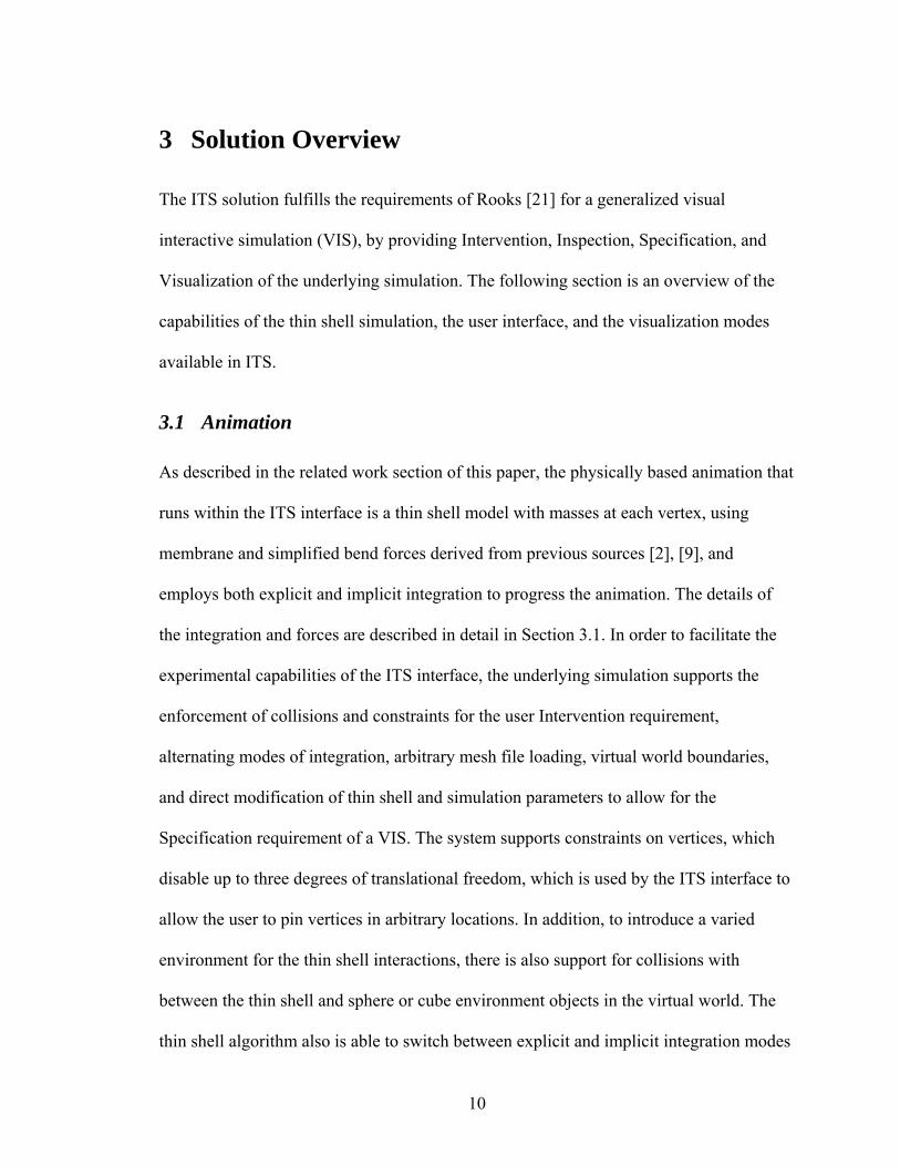
3.3.1 Dynamic Histogram

In the ITS environment, it is important that the user be able to see the various forces

acting on the vertices in the simulation, so that he or she may explore the effects of

various types of interactions on the animation. Because of this, the user may choose to

view the force values for the membrane, bend, or total forces for each vertex within the

system. When any of these views are chosen, each vertex is colored according to the

location it fits on a histogram, as pictured in Figure 1. This mapping from the large range

of possible force values to a series of discrete colors associated with ranges of these

values ensures that resulting coloring model exhibits sufficient variations among possible

force colors that are large enough to be perceived by the human eye of an ITS user. This

is important for analyzing the algorithm at hand and determining areas of interest and

performing comparative analysis of different experimental conditions.

The difference between a traditional histogram and the one in the ITS environment is its

dynamic range and force-to-color mapping capabilities, which are accomplished through

compression and equalization algorithms, respectively. Compression shifts the upper and

lower ranges of the histogram in order to attempt to equalize the number of values in each

histogram segment, while preserving the equal range increments from one segment to the

next. Equalization, on the other hand, performs a non-linear transformation on the

underlying force data points in order to spread it across the histogram equally, which

14

does not preserve the equal range size of segments and therefore relative color

comparisons are not reliable [8]. The compression algorithm cannot always choose ideal

range values to evenly spread the force values, due to the discrete nature of the

histogram, but equalization forces this to occur through a numerical transformation on the

original force data, at the expense of uniform relative histogram segment sizes.

Therefore, the compression algorithm is useful when relative comparisons between force

values must be made, and equalization is useful in discovering areas of small force

variation that do not show up on a fixed-size segment histogram. More details on the

implementation of these histogram algorithms are in Sections 4.3.1 and 4.3.2 of this

paper.

When requested by the ITS user, the compression and equalization algorithms can

analyze a single frame of force values or all frames and therefore all force values that

have been recorded and are in the simulation cache, which is described later. The analysis

of all past and present frame data results in a histogram that is optimized for an entire run

of a simulation, and has the ability to show, on average, an adequate distribution of color

for any given frame in the animation. In order to analyze all frames of force data, the

simulation cache is accessed when necessary to gain access to previously stored state

information.

15

Figure 1 - A force value histogram, with corresponding hue value mappings

3.3.2 Animation Cache

The ITS application stores a buffer of previous simulation data in a cache so that the user

may navigate to a previous time step and analyze the state of the animation. The force

coloring option may also be enabled when viewing the cache, so that previous force

values can be observed and analyzed. The buffer keeps track of the locations of all

vertices in the animation, as well as the total, membrane, and bend force vectors for each

of those vertices. In addition, the material parameter settings for each experiment at every

frame are stored in this cache, as well the time step and gravity acceleration global

settings. In this way, the user is able to see the exact progression of the animation and

determine the cause of various behaviors or manipulations in the environment. With

Force Magnitude Range Segments from Min. Force to Max Force

Values <= Min. Force Value Values >= Max. Force Value

Increasing Color Hue Value

16

access to a history of all the data that is available at the original animation runtime, useful

experiments can performed and then reanalyzed repeatedly to make useful conclusions.

17

4 Implementation

This section describes the specific implementation of features the ITS environment.

Sections 4.1 through 4.3 describe, in detail, the important or unique capabilities of our

software, which directly influence the capability of the system to fulfill the requirements

outlined in Section 2. A more complete full feature list, which outlines all major and

minor capabilities in the ITS system, is available in Section 4.4. In all mathematical

equations in this section, bolded letters signify matrix or vector variables.

4.1 Animation

The integration code of the ITS physically based animation is based on the

implementation of Baraff and Witkin’s implicit cloth simulation by Dean Marci of the

Intel Corporation [15]. It has been modified to support a new bending force described in

this section, stiffer membrane force constants to replicate the behavior of thin shells,

more complex object intersections, and adaptive integration time steps.

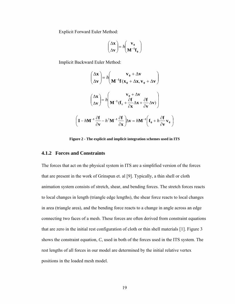
4.1.1 Implicit and Explicit Integration

The implicit and explicit integration methods that are implemented in the ITS application

are extensively discussed in many previous papers [1], [2]. The equations in Figure 2

govern the progression of our animation. The explicit forward Euler method involves the

straightforward computation of new accelerations and velocities by applying the force to

the inverted masses of all vertices in the animation, and scaling these by the current time

step, h. This method often results in a diverging system due to the extremely small step

sizes required when strong forces exist [1]. On the other hand, the implicit backward

18

Euler method involves computing the movement of the system by solving for the change

in position at a future point in time, based on the expected future forces, which must be

approximated by a linear expansion of the current forces. This method allows for much

larger time steps, handles stiff constraints effectively, and ensures that the current step is

reversible in time, which prevents against numerical divergence [1]. In order to compute

the acceleration, or ∆v, one must solve the linear system in the final equation in Figure 2.

This is performed using the Modified Conjugant Gradient Method, which is an algorithm

described in previous literature that is based on an existing implementation available

publicly [2], [15]. In our implementation, the thin shells membrane forces are strong

enough to require an explicit adaptive time step that is hundreds of times smaller than the

time step used for the implicit method, resulting in slower animation render times, and a

small amount of residual system instability that may occur under extreme force

conditions in the system.

19

Figure 2 - The explicit and implicit integration schemes used in ITS

4.1.2 Forces and Constraints

The forces that act on the physical system in ITS are a simplified version of the forces

that are present in the work of Grinspun et. al [9]. Typically, a thin shell or cloth

animation system consists of stretch, shear, and bending forces. The stretch forces reacts

to local changes in length (triangle edge lengths), the shear force reacts to local changes

in area (triangle area), and the bending force reacts to a change in angle across an edge

connecting two faces of a mesh. These forces are often derived from constraint equations

that are zero in the initial rest configuration of cloth or thin shell materials [1]. Figure 3

shows the constraint equation, C, used in both of the forces used in the ITS system. The

rest lengths of all forces in our model are determined by the initial relative vertex

positions in the loaded mesh model.

Explicit Forward Euler Method:

⎟⎟⎠

⎞⎜⎜⎝

⎛=⎟⎟

⎠

⎞⎜⎜⎝

⎛∆∆

−0

10

fMv

vx

h

Implicit Backward Euler Method:

⎟⎟⎠

⎞⎜⎜⎝

⎛∆+∆+

∆+=⎟⎟

⎠

⎞⎜⎜⎝

⎛∆∆

− vvxxfMvv

vx

001

0

,(h

⎟⎟

⎠

⎞

⎜⎜

⎝

⎛

∆∂∂

+∆∂∂

+

∆+=⎟⎟

⎠

⎞⎜⎜⎝

⎛∆∆

− )( 0 vvfx

xffM

vv

vx

1

0h

⎟⎠⎞

⎜⎝⎛

∂∂

+=∆⎟⎠⎞

⎜⎝⎛

∂∂

−∂∂

− −−−00

111 vvffMv

xfM

vfMI hhhh 2

20

In our implementation, we use very stiff linear constraints between each vertex of each

triangle, which prevent both local change in length and therefore any substantial change

in local area in such a manner that, in our case, separate stretch and shear forces are

unnecessary for achieving the realistic appearance of a thin shell material. As seen in

Figure 3, the membrane forces depend on the state of the linear constraint, as well as

user-defined membrane force constants, which are modified in the main user interface.

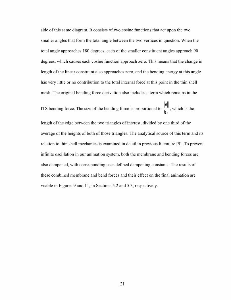
The bending force in our implementation is also a simplified form of the bending force

appearing in previous work [9]. Instead of calculating the angle change between two

faces and applying a normal force on each vertex based on this angle, a simple linear

constraint is attached to each pair of vertices that are on opposite sides of a pair of

adjacent triangles. This spring-like bending constraint mimics the function of the bending

forces found in traditional mass-spring cloth simulations based on a regular grid of

interacting particles [4]. This solution is easier to implement, and requires less

computation, but has a weakness that is made evident later in this paper. When two

triangles are nearly flat relative to each other, the resistance to bending is very weak,

because any change in the angle from this flat configuration results in very little change

in distance between the two vertices of interest, and therefore very little change in force

between these same two points. The original derivation of the bending energy did not

exhibit this weakness, due to its reliance on the angle and not linear distance between

each pair of vertices involved in the bending energy. A more technical explanation of this

weakness appears in Figure 4. On the right side of this diagram is a side view of the

bending force across two triangles. The equation for the change in the distance between

two vertices with respect to the change in angle between them appears on the bottom left

21

side of this same diagram. It consists of two cosine functions that act upon the two

smaller angles that form the total angle between the two vertices in question. When the

total angle approaches 180 degrees, each of the smaller constituent angles approach 90

degrees, which causes each cosine function approach zero. This means that the change in

length of the linear constraint also approaches zero, and the bending energy at this angle

has very little or no contribution to the total internal force at this point in the thin shell

mesh. The original bending force derivation also includes a term which remains in the

ITS bending force. The size of the bending force is proportional to eh

e, which is the

length of the edge between the two triangles of interest, divided by one third of the

average of the heights of both of those triangles. The analytical source of this term and its

relation to thin shell mechanics is examined in detail in previous literature [9]. To prevent

infinite oscillation in our animation system, both the membrane and bending forces are

also dampened, with corresponding user-defined dampening constants. The results of

these combined membrane and bend forces and their effect on the final animation are

visible in Figures 9 and 11, in Sections 5.2 and 5.3, respectively.

22

Figure 3 – The ITS Animation Membrane and Bending Forces. Membrane and bending forces have

their own force constants and dampening constants, and the bending force additionally relies upon

the length of the edge and heights of the triangles across which the force vector spans.

( )x

f∂∂

−−=CCkCk dmmMembrane a

&_

xx

xvvxf ⎟

⎟⎠

⎞⎜⎜⎝

⎛ −•−−=

)(_

abdmmMembrane kCk

a

ab MembraneMembrane ff −=

Membrane Force Bend Force Pb

Pa

x

Pb

Pa

x

e

( )x

ef

∂∂

−−=CCkCk

h dbbe

Bend a&

_

xx

xvvxe

f ⎟⎟⎠

⎞⎜⎜⎝

⎛ −•−−=

)(_

abdbb

eBend kCk

ha

ab BendBend ff −=

ab PP −=xlength) _(rest - x=C

23

Figure 4 - The Linear Bending Force Weakness. As the angle between vertices A and B flattens, the change in distance between them approaches zero.

4.1.3 Boundaries and Object Collisions

Object constraints, their relation to the integration schemes, and their implementation are

discussed by Baraff and Witkin [2]. When a vertex of a mesh enters the inside of a

collision object, or moves beyond a specified virtual world boundary, it is moved to be

just within or underneath the surface of that collision region and constrained along a

single axis perpendicular to the surface of contact with the object. If the force

perpendicular to the surface of contact is greater than a predefined contact force limit,

then the constraint is released and the vertex is allowed to move freely. This prevents the

thin shell material from entering deeply into the object of intersection, but also allows for

sliding across the region of collision. The contact force on the vertex prevents oscillation

of movement and constraint conditions on the surface of collision objects and boundaries,

and the result is more realistic animation. Figure 10, in Section 5.2 demonstrates the

visual results of these features.

X

Pb

aθ

Pa

bθ eb ea

Xb Xa

)cos(

)sin(

aaa

aaa

eddx

ex

θθ

θ

=

=

)cos()cos()(bbaa

ba eed

xxdddx θθ

θθ+=

+=

)cos(

)sin(

bbb

bbb

eddx

ex

θθ

θ

=

=

Pb

Pb

Pa

x

PbPa x

Pa

x

24

4.1.4 Adaptive Time Steps

While the implicit integration scheme in ITS is extremely stable and allows for larger

time steps and stiffer constraints, it is still possible for it to experience instability in cases

of extreme force magnitudes. Due to this potential vulnerability, and the inherent

instability of the explicit integration method, the ITS environment supports adaptive time

steps, which reduce in size in response to divergent behavior, or large changes in velocity

or position. Upon each update of the positions and velocities in the ITS simulation model,

if the change in position or velocity exceed a predefined upper bound, the changes are not

applied, the time step is cut in half, and the iteration begins again. If the extreme position

or velocity changes continue to occur, the time step is repeatedly reduced until it is no

smaller than a predefined lower bound. If divergent behavior continues to occur, the

simulation proceeds without reducing the time step, allows the errors to occur, and

notifies the ITS interface of the problem. However, if a successful iteration occurs, the

current time step, if it has been lowered, is increased a very small amount. This allows

the ITS animation algorithm to adapt to the current state of the animation automatically,

and helps to avoid significant errors in the computation.

4.2 User Interaction

As described in Section 4.1, the ITS environment allows the user to modify directly the

force constants, dampening constants, gravitational acceleration, time step size, camera

views, and environment collision object settings. The implementation of these

interactions is straightforward matter. However, the process of allowing the user to

interact directly with the animation using the mouse cursor is a more complicated

procedure, since it involves modifying the vertex locations and therefore the internal

25

forces of the thin shell materials involved. The following section discusses the details of

the methods used to allow this interaction to occur without algorithm instability and

across all experiments running simultaneously the ITS interface.

4.2.1 Live Interaction

When an animation is currently playing, the user is able to use the mouse cursor to select

and move any vertex in any experiment on the screen. Each vertex has an associated

spherical “control point”, which can be displayed on screen at the user’s discretion. This

control point is a sphere of a fixed radius that represents a volume of space that a vertex

occupies. Upon the action of clicking, the ITS interface calculates the vector associated

with the selected pixel that emanates from the camera location into the virtual world. This

is accomplished using the gluUnProject function available in the OpenGL software

library, which provides the geometry processing and rasterization framework for our

system. This vector is then tested for intersection against all control points in all

experiments and the closest intersected vertex is selected. The vector from the selected

vertex to the camera then becomes the normal component of a plane located at the

selected vertex location. When the user drags the mouse, a new linear constraint with

zero rest length is attached between two points - the selected vertex, and the point of

intersection between the mouse vector and the previously generated plane. In this

configuration, the selected vertex reacts to the attached constraint, while the user-selected

intersection point stays firmly fixed in space. The end result is that the user can enact a

constraint force and move the particle towards a location that is along a plane

perpendicular to the camera ray. This movement algorithm allows for natural interaction

that is compatible with any camera rotations or translations. Figure 12, in Section 5.3

26

later in this paper, visualizes the results of this interaction technique. The vertex of

interest cannot be directly moved by the mouse, because the movement would result in

very large changes in velocity due to instantaneous and large position changes caused by

the finite precision of the mouse location on the screen. These large changes in velocity

would potentially lead to numerical instability.

4.2.2 Paused Interaction

When the ITS animation algorithm is paused, the user may click and select any vertex

and choose to “pin” or “unpin” it. Pinning a vertex enforces a constraint with zero

degrees of freedom on the vertex of interest, and unpinning a vertex releases any

constraints that are currently enabled on that vertex. A pinned vertex cannot change

velocity or position in the virtual world. The blue sphere objects in Figure 11, in Section

5.3, represent the locations of vertices that have been pinned by the user using this

technique. The user is not able to move the positions of any vertices while the animation

is paused, because this would introduce instantaneous changes in position and therefore

very large acceleration values that would likely introduce instability in the physical

model.

4.2.3 Synchronized Interaction

Due to the experimental nature of our system, we designed the ITS system to allow

simultaneous live or paused user interaction of multiple experiments in parallel. This is

possible because all experiments share the same mesh structure. When a user performs a

live or paused interaction, the vertex that is selected in the current mesh has the same

index into the underlying data structures. Because of this, the ITS environment can easily

27

attach simultaneous constraints and simultaneous forces on all meshes. When performing

live interaction, the ITS program first calculates the interaction with the experiment that

was selected with the mouse directly, and then determines the offset of the generated

linear constraint in relation to the vertex of interest. This offset is then utilized by all

other thin shell meshes to determine the location of the linear constraint points within

their local coordinates. The result of this synchronized interaction is a more robust

experimental interface that allows very precise and identical manipulation of many

experiments in such a way that allows useful comparative analysis. A screenshot of the

process of synchronized experiment interaction is displayed in Figure 7 of Section 5.1.

4.3 Visualization

As mentioned in Section 3.3, the ITS environment allows the user to view the physical

model in two different ways in addition to the standard live rendering of the thin shell

animation. In the first way, a dynamic histogram colors the mesh surface according to the

distribution of one of three types of force values - total force, membrane force, or

bending force – for all rendered vertices, in a histogram graph that can be dynamically

adjusted according to the algorithms described below. This colorization process attempts

to render the surface of the thin shell in such a way that it is easy to determine regions of

high and low force at a glance, without resorting to the reading of numerical values on

the screen. The second view relates to the temporal progression of the animation. With a

fixed size buffer cache of all previous frames of the animation, the user has the ability to

view the past progression of the current animation, including all vertex locations, force

values, force constants, and global parameters, and use this information to analyze the

effects of each of these animation parameters over time.

28

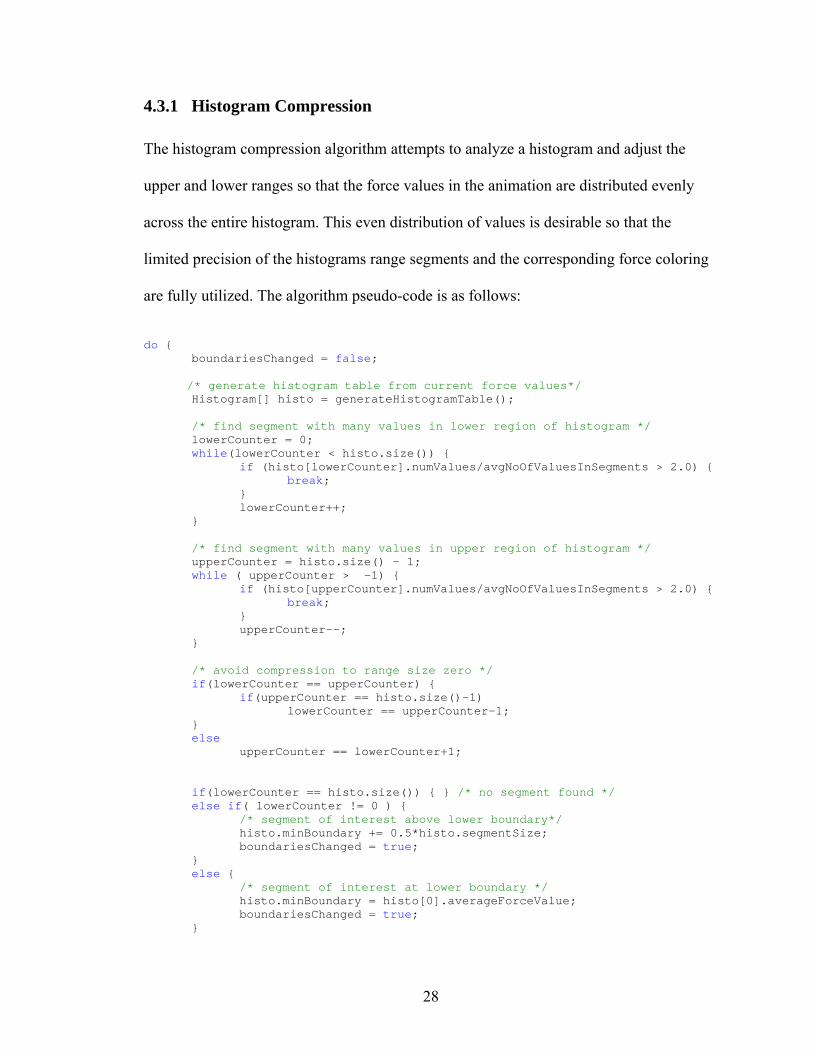
4.3.1 Histogram Compression

The histogram compression algorithm attempts to analyze a histogram and adjust the

upper and lower ranges so that the force values in the animation are distributed evenly

across the entire histogram. This even distribution of values is desirable so that the

limited precision of the histograms range segments and the corresponding force coloring

are fully utilized. The algorithm pseudo-code is as follows:

do { boundariesChanged = false; /* generate histogram table from current force values*/ Histogram[] histo = generateHistogramTable(); /* find segment with many values in lower region of histogram */ lowerCounter = 0; while(lowerCounter < histo.size()) { if (histo[lowerCounter].numValues/avgNoOfValuesInSegments > 2.0) { break; } lowerCounter++; } /* find segment with many values in upper region of histogram */ upperCounter = histo.size() – 1; while ( upperCounter > -1) { if (histo[upperCounter].numValues/avgNoOfValuesInSegments > 2.0) { break; } upperCounter--; } /* avoid compression to range size zero */ if(lowerCounter == upperCounter) { if(upperCounter == histo.size()-1) lowerCounter == upperCounter–1; } else upperCounter == lowerCounter+1; if(lowerCounter == histo.size()) { } /* no segment found */ else if( lowerCounter != 0 ) { /* segment of interest above lower boundary*/ histo.minBoundary += 0.5*histo.segmentSize; boundariesChanged = true; } else { /* segment of interest at lower boundary */ histo.minBoundary = histo[0].averageForceValue; boundariesChanged = true; }

29

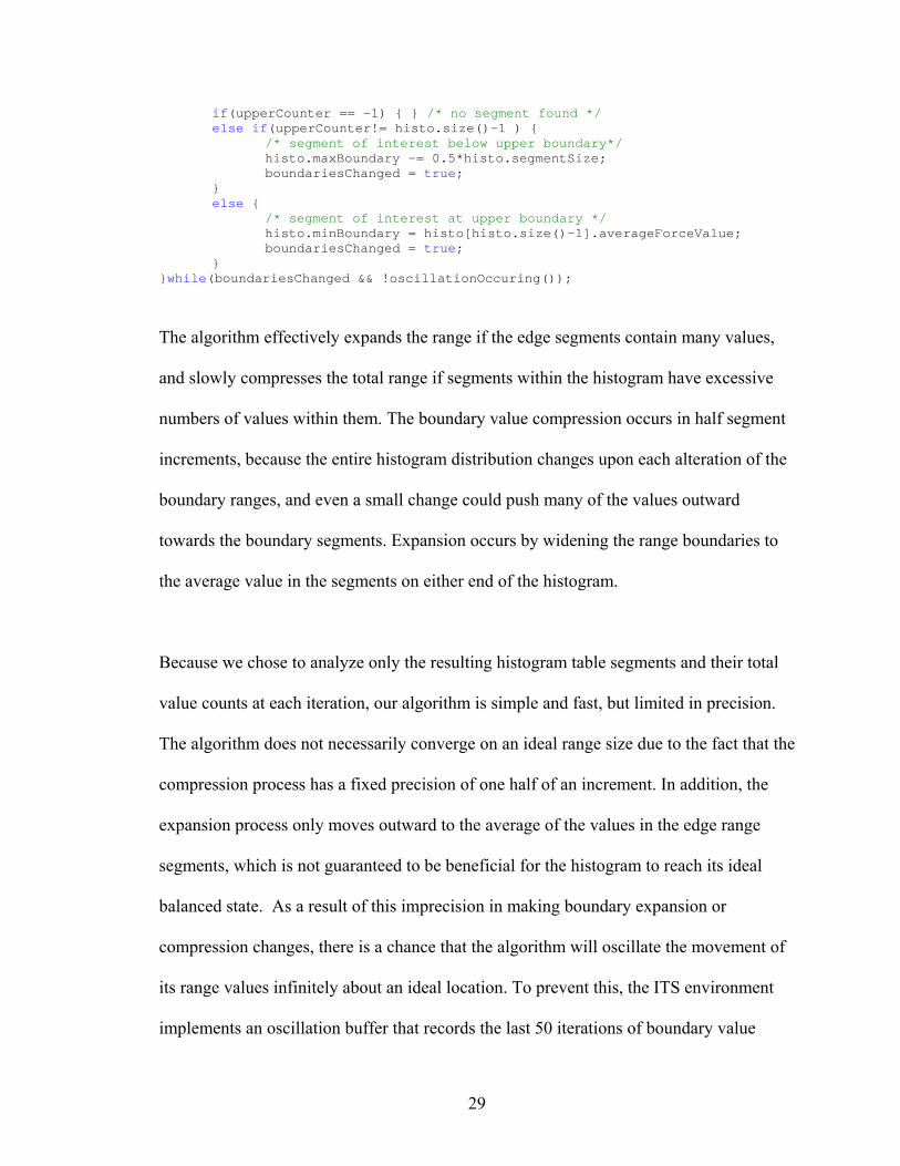
if(upperCounter == -1) { } /* no segment found */ else if(upperCounter!= histo.size()-1 ) { /* segment of interest below upper boundary*/ histo.maxBoundary -= 0.5*histo.segmentSize; boundariesChanged = true; } else { /* segment of interest at upper boundary */ histo.minBoundary = histo[histo.size()-1].averageForceValue; boundariesChanged = true; } }while(boundariesChanged && !oscillationOccuring());

The algorithm effectively expands the range if the edge segments contain many values,

and slowly compresses the total range if segments within the histogram have excessive

numbers of values within them. The boundary value compression occurs in half segment

increments, because the entire histogram distribution changes upon each alteration of the

boundary ranges, and even a small change could push many of the values outward

towards the boundary segments. Expansion occurs by widening the range boundaries to

the average value in the segments on either end of the histogram.

Because we chose to analyze only the resulting histogram table segments and their total

value counts at each iteration, our algorithm is simple and fast, but limited in precision.

The algorithm does not necessarily converge on an ideal range size due to the fact that the

compression process has a fixed precision of one half of an increment. In addition, the

expansion process only moves outward to the average of the values in the edge range

segments, which is not guaranteed to be beneficial for the histogram to reach its ideal

balanced state. As a result of this imprecision in making boundary expansion or

compression changes, there is a chance that the algorithm will oscillate the movement of

its range values infinitely about an ideal location. To prevent this, the ITS environment

implements an oscillation buffer that records the last 50 iterations of boundary value

30

adjustments. If the average change recorded in this buffer approaches zero for both the

upper and lower boundary, then oscillation is detected and the algorithm is stopped.

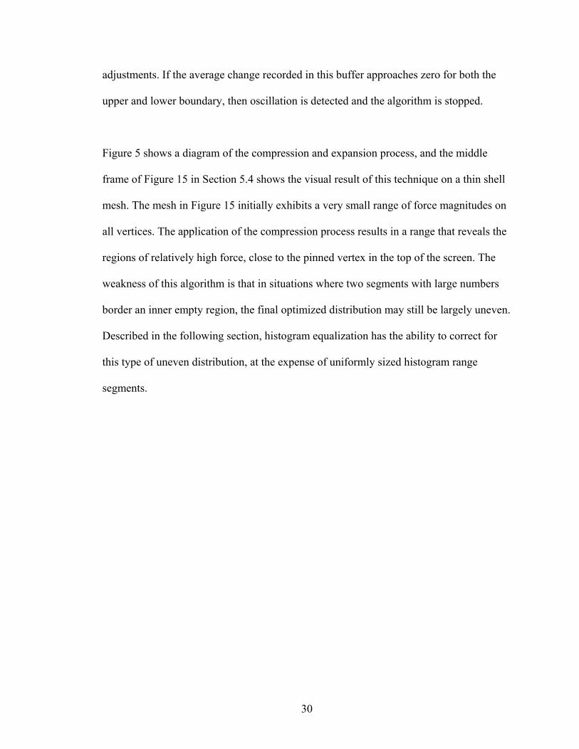
Figure 5 shows a diagram of the compression and expansion process, and the middle

frame of Figure 15 in Section 5.4 shows the visual result of this technique on a thin shell

mesh. The mesh in Figure 15 initially exhibits a very small range of force magnitudes on

all vertices. The application of the compression process results in a range that reveals the

regions of relatively high force, close to the pinned vertex in the top of the screen. The

weakness of this algorithm is that in situations where two segments with large numbers

border an inner empty region, the final optimized distribution may still be largely uneven.

Described in the following section, histogram equalization has the ability to correct for

this type of uneven distribution, at the expense of uniformly sized histogram range

segments.

31

Figure 5 - The ITS histogram compression algorithm.

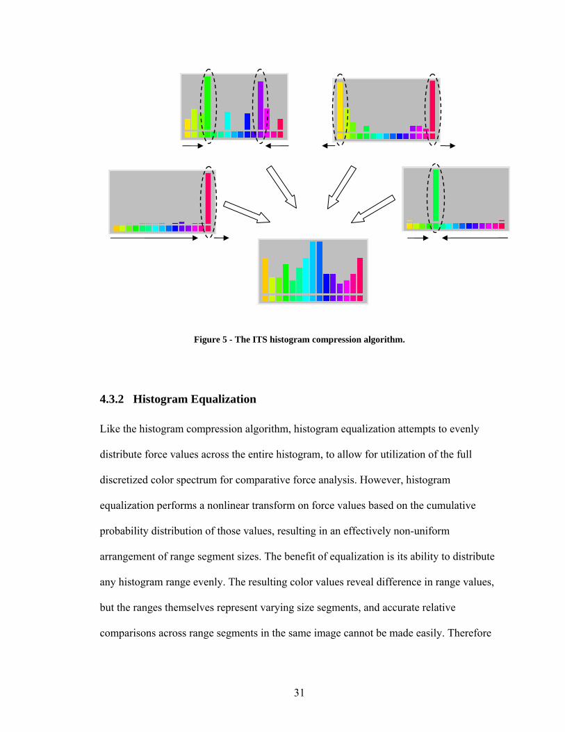
4.3.2 Histogram Equalization

Like the histogram compression algorithm, histogram equalization attempts to evenly

distribute force values across the entire histogram, to allow for utilization of the full

discretized color spectrum for comparative force analysis. However, histogram

equalization performs a nonlinear transform on force values based on the cumulative

probability distribution of those values, resulting in an effectively non-uniform

arrangement of range segment sizes. The benefit of equalization is its ability to distribute

any histogram range evenly. The resulting color values reveal difference in range values,

but the ranges themselves represent varying size segments, and accurate relative

comparisons across range segments in the same image cannot be made easily. Therefore

32

equalization serves to more effectively optimize the use of the histogram and its range of

color, at the expense of accurate force value comparisons.

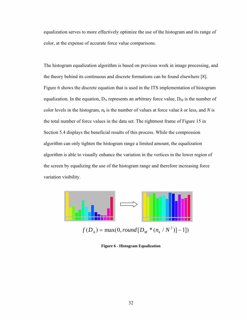
The histogram equalization algorithm is based on previous work in image processing, and

the theory behind its continuous and discrete formations can be found elsewhere [8].

Figure 6 shows the discrete equation that is used in the ITS implementation of histogram

equalization. In the equation, DA represents an arbitrary force value, DM is the number of

color levels in the histogram, nk is the number of values at force value k or less, and N is

the total number of force values in the data set. The rightmost frame of Figure 15 in

Section 5.4 displays the beneficial results of this process. While the compression

algorithm can only tighten the histogram range a limited amount, the equalization

algorithm is able to visually enhance the variation in the vertices in the lower region of

the screen by equalizing the use of the histogram range and therefore increasing force

variation visibility.

Figure 6 - Histogram Equalization

])1)]/(*[,0max()( 2 −= NnDroundDf kMA

33

4.3.3 Animation Cache

The cache of data that stores the history of the current animation can be accessed directly

from the main ITS user interface. The cache is a fixed size buffer. If it is filled, the

current frame information overwrites the oldest frame information, and the boundaries of

the buffer are updated internally. The main user interface presents an interface to the

animation cache as a slider bar and a series of buttons that control navigation through the

cache data. The slider represents the current information in the buffer, and the rightmost

position on it is always the latest cache data. To achieve this translation from a graphical

element to an internal data structure, the ITS program must convert the requested

progress percentage across the slider bar into an index in the internal data structure. This

process must take into account the circular nature of the buffer and ensure that all offsets

are valid. The main ITS interface has the ability to request the next or previous frame

from given a current frame index received from the buffer at an earlier time, or specify

any arbitrary buffer location using a percentage value as a request parameter.

4.4 Full Feature List

The ITS environment is written in C++ and OpenGL, and makes use of the GLUI

graphical user interface library [18]. Because there are many features of the ITS

environment which are minor in nature, but contribute to the user experience as a whole,

we have compiled a list of all the features that are available in the ITS environment, as

follows:

34

Animation Features o Implicit integration with the Modified Conjugant Gradient Method

o Explicit integration

o Adaptive time step

o Arbitrary mesh file support

o Vertex constraints with 1, 2, and 3 degrees of freedom

o Vertex-sphere and vertex-cube collision detection

User-controlled Parameters o Gravitational acceleration

o Total mesh weight

o Desired time step size

o Membrane force constant per experiment

o Membrane force dampening constant per experiment

o Bend force constant per experiment

o Bend force dampening constant per experiment

o Location and existence of three environment collision objects: two spheres and a cube

o Camera rotation and translation

User Interaction o Playing and pausing of animation

o Pinning and unpinning of vertices in a paused animation

o Spring-based interaction with vertices a playing animation

o Synchronized interaction across all experiments

o Navigation of simulation cache: play, pause, first frame, last frame, next frame, previous frame

Visualization o Simultaneous mesh experiments

o Membrane force coloring, direction vectors

o Bend force coloring, direction vectors

o Total force coloring, direction vectors

o Large control points on each vertex

o Adaptive time step size per experiment

o Histogram force distribution for current frame

35

o Current histogram force range values

o Optimized compressed histogram range

o Equalized histogram values

o Wire frame rendering

o Visible or invisible environment collision objects

36

5 Results

In this section, we will highlight some of the important features of the ITS environment

that allow it to act as a truly free form experimental environment. Many of the features

implemented in the ITS environment, such as adaptive time steps, camera view

modification, and animation cache navigation, are difficult to demonstrate with still

screenshots, but are completely functional in the implementation.

5.1 User Interface Overview

The main ITS user interface is displayed in Figure 7. In this screenshot, a user is

interacting with four simultaneous experiments with varying strengths of membrane and

bending forces, and has histogram force coloring enabled. When a user loads up the

program, he or she uses the buttons in region A of the screen to select the total mesh

weight and load an arbitrary mesh. Region B of the image outlines the region of the

interface where the user can modify any of the force or dampening parameters for each of

the experiments. Region C contains the view controls which can rotate each experiment

independently on its own axis, or rotate the entire group of experiments at once. Region

D is where the user is able to control the progress of the animation algorithm. In this area,

the user can play and pause the animation, reset the experiments and global parameters

back to their original initial conditions, or restart the animation system and reload an

entirely new mesh for experimentation. Region E outlines the group of global controls

which allow the user to alter the gravitational acceleration or time step, enable or disable

the displayed cube and sphere environment collision objects, enable or disable the

rendering of force vectors to augment the force coloring, and enable or disable wire

37

frame rendering. Region F houses the controls for the dynamic histogram capabilities in

ITS. From this location in the interface, the user can enable force coloring, select the

forces to be represented on the screen, and reset, compress, or equalize the histogram for

the current frame or all recorded frames. Region G highlights the visual representation of

the force histogram, as discussed in Section 4.3. At the bottom, region H outlines the

group of controls that allow the user to play back cached animation data, and select any

frame of interest for further analysis. Finally, region I marks the visual cues for the

current adaptive time step status. Each of these bars represents the size of the current time

step for each experiment on screen, in relation to the requested time step indicated in the

global preferences panel on the right side of the screen. If the bar is full, then the current

step size is equal to the requested step size.

Figure 7 - The ITS Graphical User Interface

A

B

C

D

E

F

G

H

I

38

5.2 Animation Features

While the explicit and implicit integration capabilities are fully functional, screenshots

would not help to convey the results of the implementation. As expected, the explicit

mode requires an extremely small adaptive time step, on the order of 0.00001 seconds,

1/100th the size of the implicit mode time step, in order to keep the animation stable with

high membrane and bending force coefficients. Figure 8 shows the loading of various

arbitrary mesh files. The classic bunny model in the middle has no color assignment

embedded in its mesh file, so it is rendered with a default powder blue coloring. In this

screenshot, the green dots represent the locations of vertices on the model, and also serve

as a representation of the control points of user interaction during live and paused

animation states. Figure 9 demonstrates a set of simultaneous experiments with varying

membrane and bending force constants. Each displayed experiment is shown at the same

moment in time, and demonstrates varying reactions to collisions or pinned vertex

constraints.

Figure 8 - ITS supports arbitrary mesh files.

39

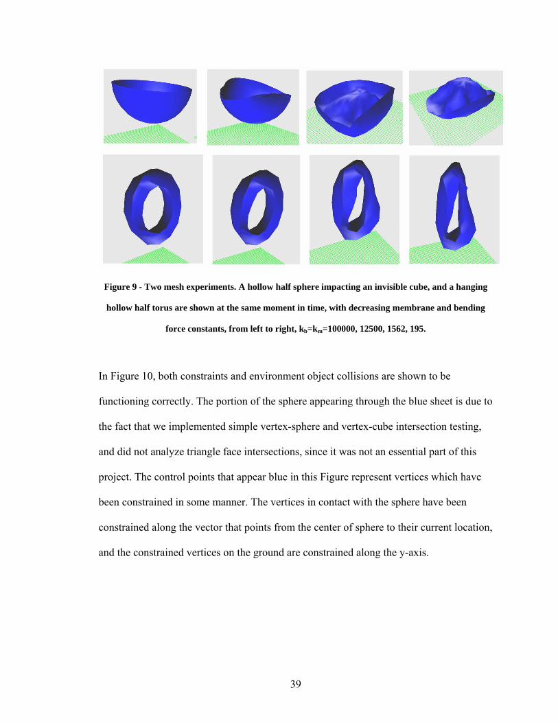
Figure 9 - Two mesh experiments. A hollow half sphere impacting an invisible cube, and a hanging

hollow half torus are shown at the same moment in time, with decreasing membrane and bending

force constants, from left to right, kb=km=100000, 12500, 1562, 195.

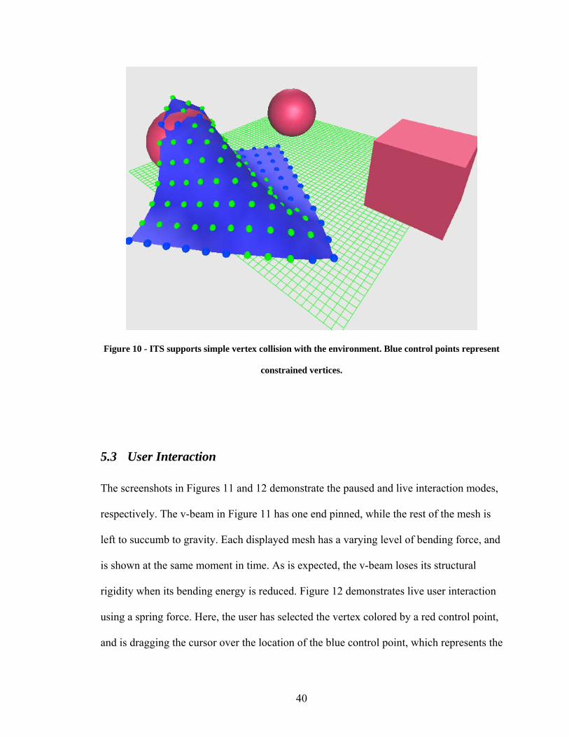
In Figure 10, both constraints and environment object collisions are shown to be

functioning correctly. The portion of the sphere appearing through the blue sheet is due to

the fact that we implemented simple vertex-sphere and vertex-cube intersection testing,

and did not analyze triangle face intersections, since it was not an essential part of this

project. The control points that appear blue in this Figure represent vertices which have

been constrained in some manner. The vertices in contact with the sphere have been

constrained along the vector that points from the center of sphere to their current location,

and the constrained vertices on the ground are constrained along the y-axis.

40

Figure 10 - ITS supports simple vertex collision with the environment. Blue control points represent

constrained vertices.

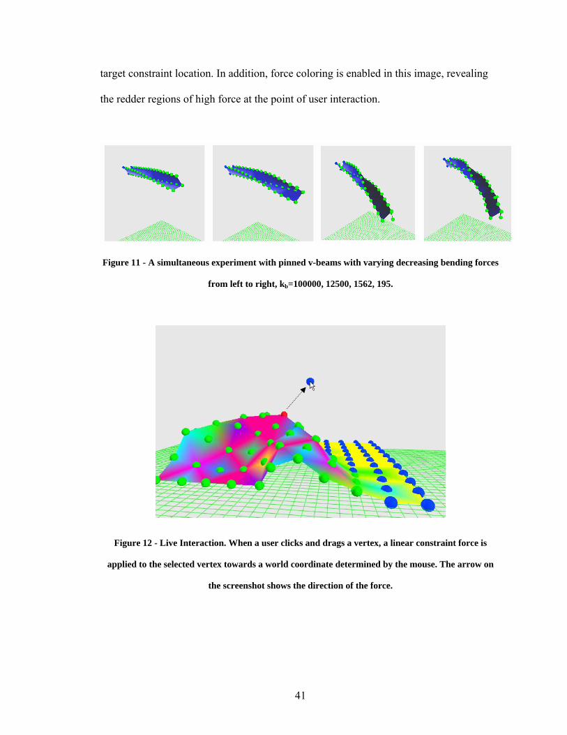
5.3 User Interaction

The screenshots in Figures 11 and 12 demonstrate the paused and live interaction modes,

respectively. The v-beam in Figure 11 has one end pinned, while the rest of the mesh is

left to succumb to gravity. Each displayed mesh has a varying level of bending force, and

is shown at the same moment in time. As is expected, the v-beam loses its structural

rigidity when its bending energy is reduced. Figure 12 demonstrates live user interaction

using a spring force. Here, the user has selected the vertex colored by a red control point,

and is dragging the cursor over the location of the blue control point, which represents the

41

target constraint location. In addition, force coloring is enabled in this image, revealing

the redder regions of high force at the point of user interaction.

Figure 11 - A simultaneous experiment with pinned v-beams with varying decreasing bending forces

from left to right, kb=100000, 12500, 1562, 195.

Figure 12 - Live Interaction. When a user clicks and drags a vertex, a linear constraint force is

applied to the selected vertex towards a world coordinate determined by the mouse. The arrow on

the screenshot shows the direction of the force.

42

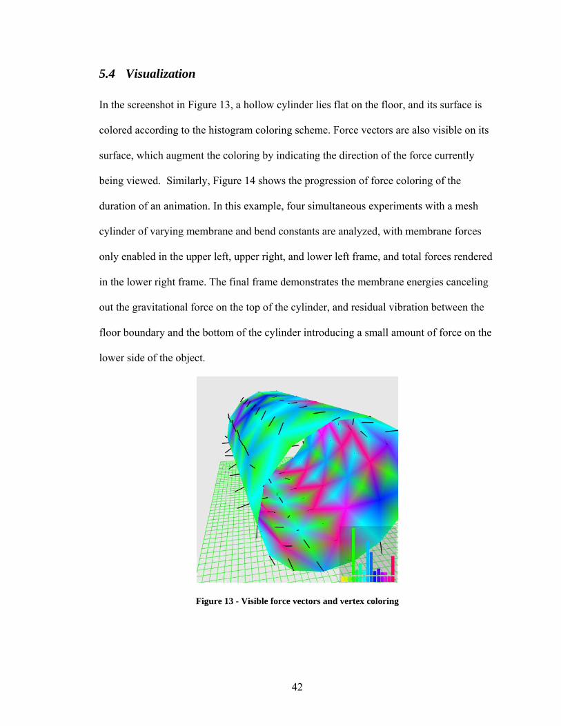
5.4 Visualization

In the screenshot in Figure 13, a hollow cylinder lies flat on the floor, and its surface is

colored according to the histogram coloring scheme. Force vectors are also visible on its

surface, which augment the coloring by indicating the direction of the force currently

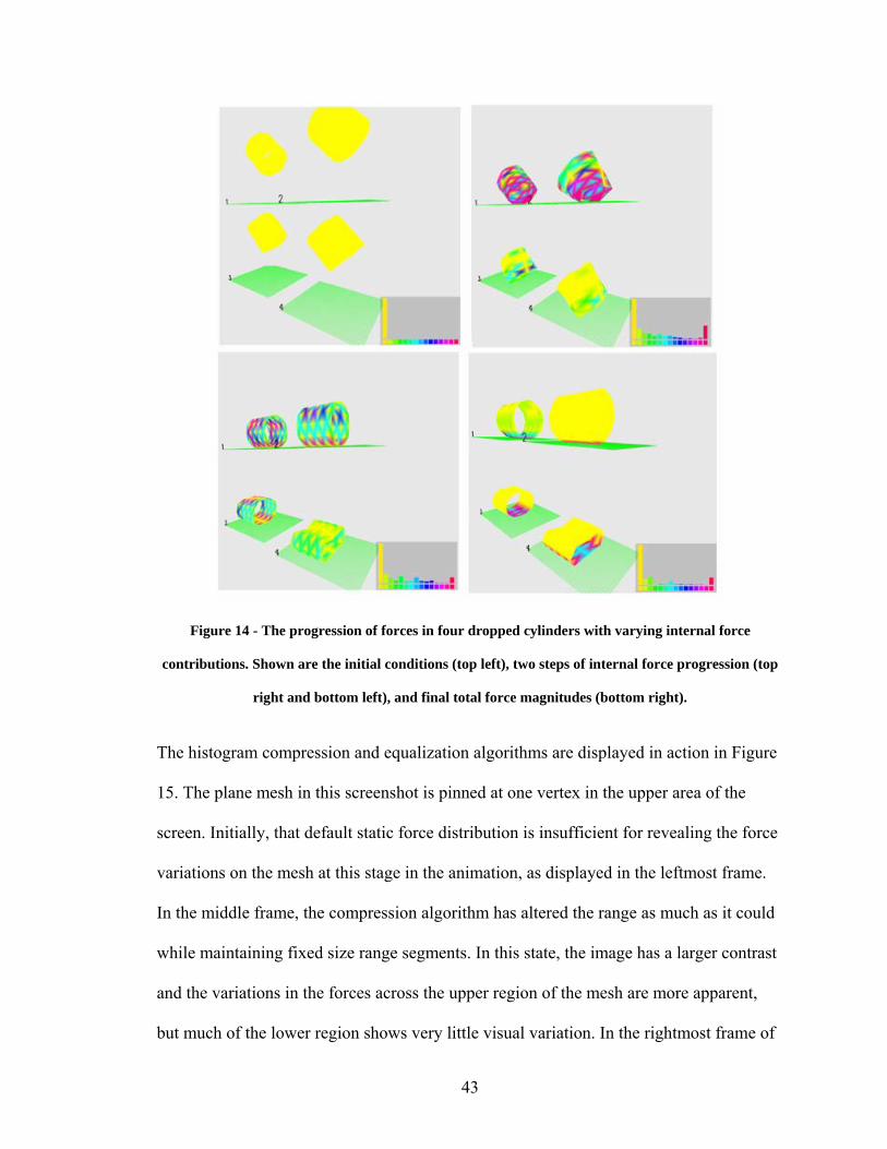
being viewed. Similarly, Figure 14 shows the progression of force coloring of the

duration of an animation. In this example, four simultaneous experiments with a mesh

cylinder of varying membrane and bend constants are analyzed, with membrane forces

only enabled in the upper left, upper right, and lower left frame, and total forces rendered

in the lower right frame. The final frame demonstrates the membrane energies canceling

out the gravitational force on the top of the cylinder, and residual vibration between the

floor boundary and the bottom of the cylinder introducing a small amount of force on the

lower side of the object.

Figure 13 - Visible force vectors and vertex coloring

43

Figure 14 - The progression of forces in four dropped cylinders with varying internal force

contributions. Shown are the initial conditions (top left), two steps of internal force progression (top

right and bottom left), and final total force magnitudes (bottom right).

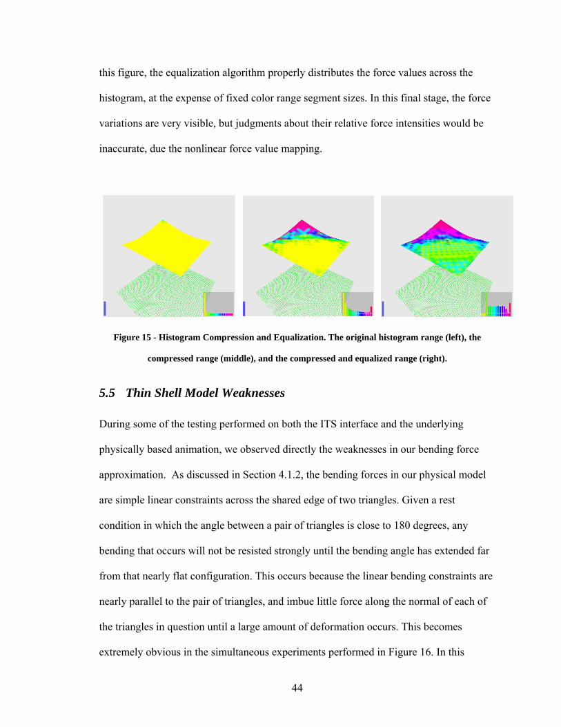
The histogram compression and equalization algorithms are displayed in action in Figure

15. The plane mesh in this screenshot is pinned at one vertex in the upper area of the

screen. Initially, that default static force distribution is insufficient for revealing the force

variations on the mesh at this stage in the animation, as displayed in the leftmost frame.

In the middle frame, the compression algorithm has altered the range as much as it could

while maintaining fixed size range segments. In this state, the image has a larger contrast

and the variations in the forces across the upper region of the mesh are more apparent,

but much of the lower region shows very little visual variation. In the rightmost frame of

44

this figure, the equalization algorithm properly distributes the force values across the

histogram, at the expense of fixed color range segment sizes. In this final stage, the force

variations are very visible, but judgments about their relative force intensities would be

inaccurate, due the nonlinear force value mapping.

Figure 15 - Histogram Compression and Equalization. The original histogram range (left), the

compressed range (middle), and the compressed and equalized range (right).

5.5 Thin Shell Model Weaknesses

During some of the testing performed on both the ITS interface and the underlying

physically based animation, we observed directly the weaknesses in our bending force

approximation. As discussed in Section 4.1.2, the bending forces in our physical model

are simple linear constraints across the shared edge of two triangles. Given a rest

condition in which the angle between a pair of triangles is close to 180 degrees, any

bending that occurs will not be resisted strongly until the bending angle has extended far

from that nearly flat configuration. This occurs because the linear bending constraints are

nearly parallel to the pair of triangles, and imbue little force along the normal of each of

the triangles in question until a large amount of deformation occurs. This becomes

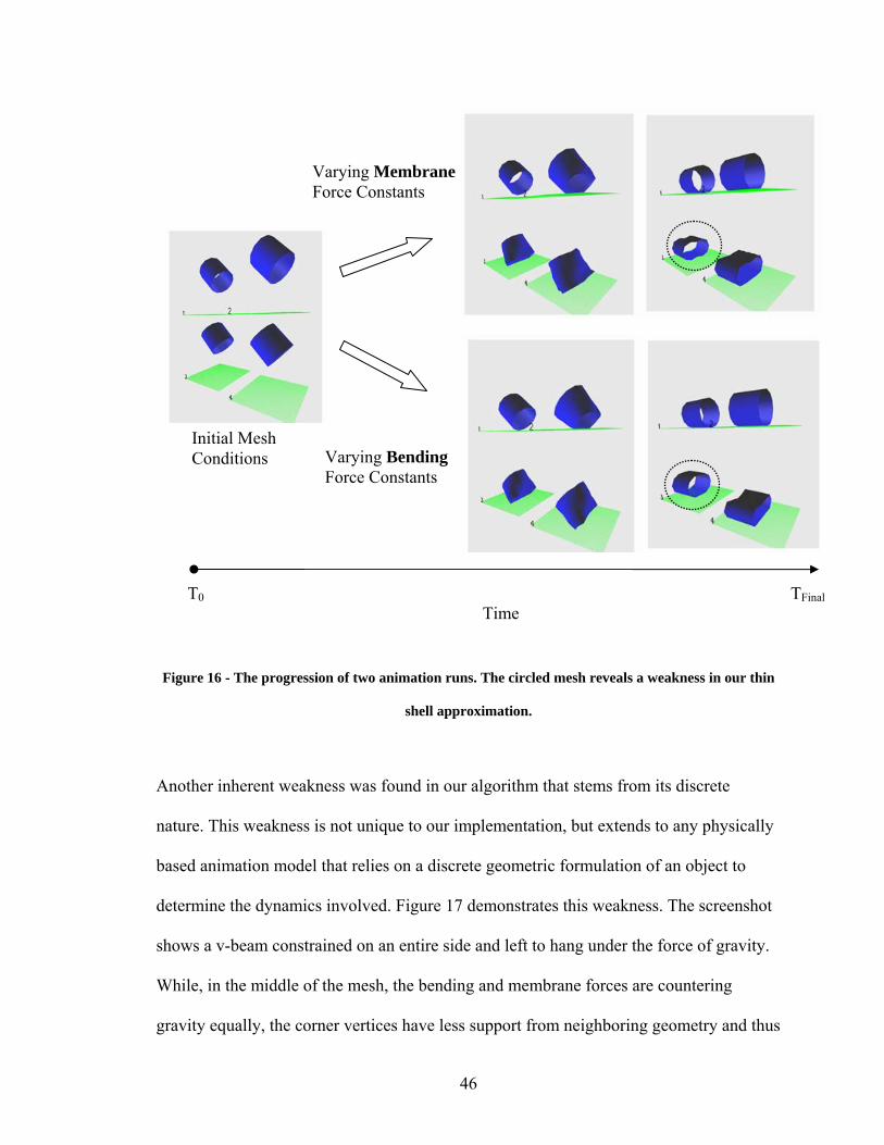
extremely obvious in the simultaneous experiments performed in Figure 16. In this

45

Figure, two sets of experiments are run. In the upper set, the bending constraints were

kept equal and the membrane forces were decrease in order of left to right and top to

bottom. In the lower set, the membrane force constraints are kept constant, and bending

forces are reduced. Given equal bending force constants, the upper set of panels shows

that when the membrane force is low, the bending force is the primary source of

structural integrity. When this occurs, the bending force cannot withstand the

gravitational force on the top of the cylinder, and the faces along the top invert their

angle. This occurs because the initial configuration of the cylinder generates bending

constraints that are all nearly 180 degrees, and therefore weak until significant

deformation occurs. In the bottom set of panels, the membrane force is equal amongst all

experiments, and prevents the angle inversion from occurring, showing that the bending

force in the cylinder model contributes very little in these experiments, due to the high

angles between all the faces of the mesh.

46

Figure 16 - The progression of two animation runs. The circled mesh reveals a weakness in our thin

shell approximation.

Another inherent weakness was found in our algorithm that stems from its discrete

nature. This weakness is not unique to our implementation, but extends to any physically

based animation model that relies on a discrete geometric formulation of an object to

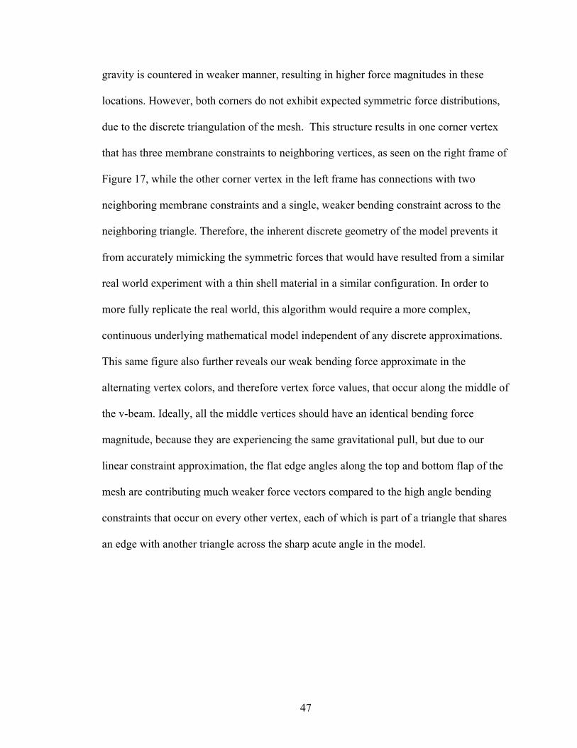
determine the dynamics involved. Figure 17 demonstrates this weakness. The screenshot

shows a v-beam constrained on an entire side and left to hang under the force of gravity.

While, in the middle of the mesh, the bending and membrane forces are countering

gravity equally, the corner vertices have less support from neighboring geometry and thus

Initial Mesh Conditions

Varying Membrane Force Constants

T0 TFinal Time

Varying Bending Force Constants

47

gravity is countered in weaker manner, resulting in higher force magnitudes in these

locations. However, both corners do not exhibit expected symmetric force distributions,

due to the discrete triangulation of the mesh. This structure results in one corner vertex

that has three membrane constraints to neighboring vertices, as seen on the right frame of

Figure 17, while the other corner vertex in the left frame has connections with two

neighboring membrane constraints and a single, weaker bending constraint across to the

neighboring triangle. Therefore, the inherent discrete geometry of the model prevents it

from accurately mimicking the symmetric forces that would have resulted from a similar

real world experiment with a thin shell material in a similar configuration. In order to

more fully replicate the real world, this algorithm would require a more complex,

continuous underlying mathematical model independent of any discrete approximations.

This same figure also further reveals our weak bending force approximate in the

alternating vertex colors, and therefore vertex force values, that occur along the middle of

the v-beam. Ideally, all the middle vertices should have an identical bending force

magnitude, because they are experiencing the same gravitational pull, but due to our

linear constraint approximation, the flat edge angles along the top and bottom flap of the

mesh are contributing much weaker force vectors compared to the high angle bending

constraints that occur on every other vertex, each of which is part of a triangle that shares

an edge with another triangle across the sharp acute angle in the model.

48

Figure 17 - Unrealistic Forces. Two panels (left, right) show bending force views of two sides of the

same experiment on a v-beam with pinned vertices. The forces are asymmetric due to the underlying

triangulation of the mesh. The black lines indicate triangle edges.

5.6 Performance

The ITS environment uses a large amount of memory to store animation cache data, and

performs a large number of mathematical operations per iteration, resulting in a

simulation that has some very obvious performance weaknesses. On our test system,

which is an Athlon 64 3500+, with 1 GB RAM, and an ATI Radeon X850XT graphics

card, the simulation became unusable, with non-interactive frame rates, at approximately

1200 vertices on screen at once. Our tests were performed with a 1300 frame cache. Each

frame of data occupies approximately 125 bytes per vertex. In terms of memory usage,

with the establish 1300 frame cache, one gigabyte of memory will be occupied by purely

frame data when approximately 6614 vertices are rendered on screen at once. According

to these calculations, the simulation on our test machine is primarily limited by its

calculation speed, as opposed to its memory footprint. These testing results are limited to

a single computer and therefore are useful only for grasping a general idea of the level of

performance that is achieved with this application. Due to the fact that the ITS

49

environment and its thin shell model were constructed to demonstrate a unique tool with

no known comparable implementations, it was not constructed with optimization and

competitive performance analysis in mind. In addition, much of the computational limits

of the ITS system arise due to the specific implementation of the thin shells model, which

is not the core focus of this paper. Because of both of these reasons, there is likely much

room for both memory and computation optimization throughout the program.

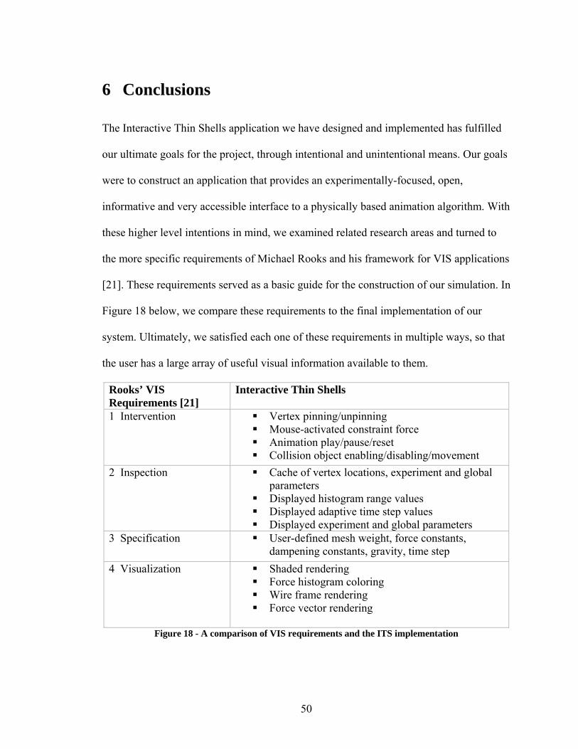
50

6 Conclusions

The Interactive Thin Shells application we have designed and implemented has fulfilled

our ultimate goals for the project, through intentional and unintentional means. Our goals

were to construct an application that provides an experimentally-focused, open,

informative and very accessible interface to a physically based animation algorithm. With

these higher level intentions in mind, we examined related research areas and turned to

the more specific requirements of Michael Rooks and his framework for VIS applications

[21]. These requirements served as a basic guide for the construction of our simulation. In

Figure 18 below, we compare these requirements to the final implementation of our

system. Ultimately, we satisfied each one of these requirements in multiple ways, so that

the user has a large array of useful visual information available to them.

Rooks’ VIS Requirements [21]

Interactive Thin Shells

1 Intervention Vertex pinning/unpinning Mouse-activated constraint force Animation play/pause/reset Collision object enabling/disabling/movement

2 Inspection Cache of vertex locations, experiment and global parameters

Displayed histogram range values Displayed adaptive time step values Displayed experiment and global parameters

3 Specification User-defined mesh weight, force constants, dampening constants, gravity, time step

4 Visualization Shaded rendering Force histogram coloring Wire frame rendering Force vector rendering

Figure 18 - A comparison of VIS requirements and the ITS implementation

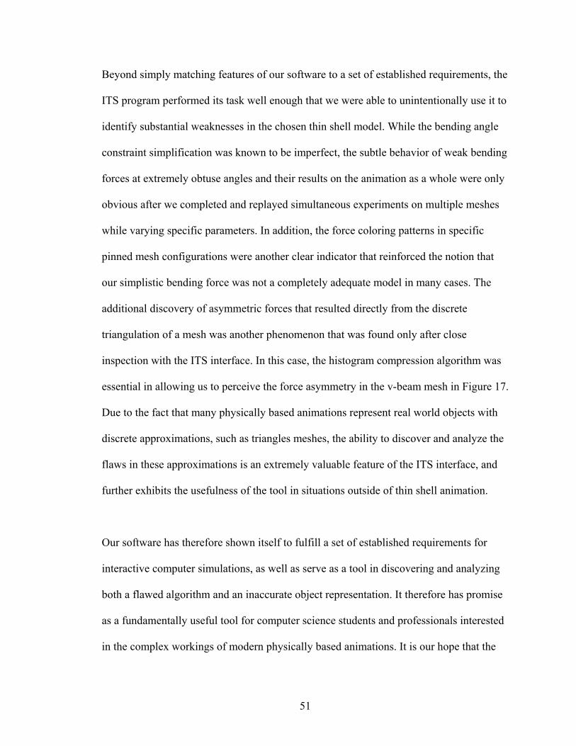
51

Beyond simply matching features of our software to a set of established requirements, the

ITS program performed its task well enough that we were able to unintentionally use it to

identify substantial weaknesses in the chosen thin shell model. While the bending angle

constraint simplification was known to be imperfect, the subtle behavior of weak bending

forces at extremely obtuse angles and their results on the animation as a whole were only

obvious after we completed and replayed simultaneous experiments on multiple meshes

while varying specific parameters. In addition, the force coloring patterns in specific

pinned mesh configurations were another clear indicator that reinforced the notion that

our simplistic bending force was not a completely adequate model in many cases. The

additional discovery of asymmetric forces that resulted directly from the discrete

triangulation of a mesh was another phenomenon that was found only after close

inspection with the ITS interface. In this case, the histogram compression algorithm was

essential in allowing us to perceive the force asymmetry in the v-beam mesh in Figure 17.

Due to the fact that many physically based animations represent real world objects with

discrete approximations, such as triangles meshes, the ability to discover and analyze the

flaws in these approximations is an extremely valuable feature of the ITS interface, and

further exhibits the usefulness of the tool in situations outside of thin shell animation.

Our software has therefore shown itself to fulfill a set of established requirements for

interactive computer simulations, as well as serve as a tool in discovering and analyzing

both a flawed algorithm and an inaccurate object representation. It therefore has promise

as a fundamentally useful tool for computer science students and professionals interested

in the complex workings of modern physically based animations. It is our hope that the

52

interface features of the ITS system will help to guide the development of similar

interactive interfaces for more complex physically based models. There is no doubt there

are a large number of animation algorithms in existence that could benefit from a more

tactile and experimental interface which can help to clear the muddled waters of abstract

mathematics and help bring it into the light of intuitive experience.

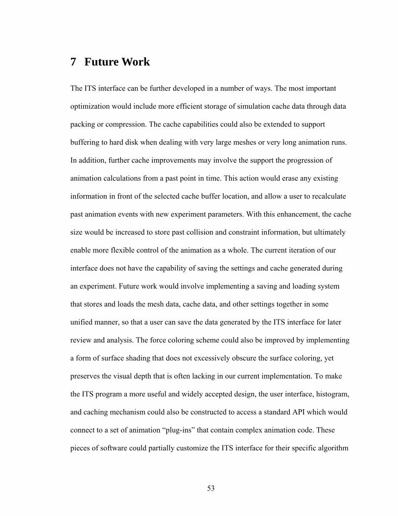
53

7 Future Work

The ITS interface can be further developed in a number of ways. The most important

optimization would include more efficient storage of simulation cache data through data

packing or compression. The cache capabilities could also be extended to support

buffering to hard disk when dealing with very large meshes or very long animation runs.

In addition, further cache improvements may involve the support the progression of

animation calculations from a past point in time. This action would erase any existing

information in front of the selected cache buffer location, and allow a user to recalculate

past animation events with new experiment parameters. With this enhancement, the cache

size would be increased to store past collision and constraint information, but ultimately

enable more flexible control of the animation as a whole. The current iteration of our

interface does not have the capability of saving the settings and cache generated during

an experiment. Future work would involve implementing a saving and loading system

that stores and loads the mesh data, cache data, and other settings together in some

unified manner, so that a user can save the data generated by the ITS interface for later

review and analysis. The force coloring scheme could also be improved by implementing

a form of surface shading that does not excessively obscure the surface coloring, yet

preserves the visual depth that is often lacking in our current implementation. To make

the ITS program a more useful and widely accepted design, the user interface, histogram,

and caching mechanism could also be constructed to access a standard API which would

connect to a set of animation “plug-ins” that contain complex animation code. These

pieces of software could partially customize the ITS interface for their specific algorithm

54

parameters. In this way, the ITS design would be a truly generalized and accessible

interface for a large assortment of mathematically intensive animation models. The

underlying thin shells simulation itself can also be greatly improved. Primarily, it would

benefit from more optimization time. Many of the underlying matrix and vector

mathematics could be offloaded to the highly parallel graphics processors so prevalent in

home computers today [19]. Furthermore, the thin shells model could be modified to

completely implement the more accurate discrete shells model of Grinspun et al [9], and

therefore provide a more realistic animation of thin shell materials.

55

8 Bibliography [1] Baraff, D. & Witkin, A. (2001), 'Physically Based Modeling', Siggraph 2001

Course Notes. [2] Baraff, D. & Witkin, A. (1998),Large steps in cloth simulation, in 'SIGGRAPH

'98: Proceedings of the 25th annual conference on Computer graphics and interactive techniques', ACM Press, New York, NY, USA, pp. 43--54.

[3] Beaubouef, T. & Mason, J. (2005),'Why the high attrition rate for computer

science students: some thoughts and observations', SIGCSE Bull. 37(2), ACM Press, New York, NY, USA, 103--106.

[4] Breen, D.E.; House, D.H. & Wozny, M.J. (1994),Predicting the drape of woven

cloth using interacting particles, in 'SIGGRAPH '94: Proceedings of the 21st annual conference on Computer graphics and interactive techniques', ACM Press, New York, NY, USA, pp. 365--372.

[5] Burgoon, R.J. (2005),'Discrete Shells Origami', Master's thesis, California

Polytechnic State University San Luis Obispo. [6] D'Antonio, L.; Baldwin, D.; Ford, F.; Henderson, P. & Wyatt, R. (2002),'Panel: is

there too much math in the computer science curriculum?', J. Comput. Small Coll. 17(3), Consortium for Computing Sciences in Colleges, , USA, 97--102.

[7] Feynman, C. (1986),'Modeling the Appearance of Cloth', Master's thesis,

Massachusetts Inst. of Technology. [8] Fisher, R.; Perkins, S.; Walker, A. & Wolfart, E. (2003),'The Hypermedia Image

Processing Reference', http://homepages.inf.ed.ac.uk/rbf/HIPR2/. [9] Grinspun, E.; Hirani, A.N.; Desbrun, M. & Schröder, P. (2003),Discrete shells, in

'SCA '03: Proceedings of the 2003 ACM SIGGRAPH/Eurographics symposium on Computer animation', Eurographics Association, Aire-la-Ville, Switzerland, Switzerland, pp. 62--67.

[10] Hoppe, H. (2006),'.M Mesh File Format', http://research.microsoft.com/~hoppe/. [11] Igarashi, T. & Hughes, J.F. (2002),Clothing manipulation, in 'UIST '02:

Proceedings of the 15th annual ACM symposium on User interface software and technology', ACM Press, New York, NY, USA, pp. 91--100.

[12] Konvalina, J.; Wileman, S.A. & Stephens, L.J. (1983), 'Math proficiency: a key to

success for computer science students', Commun. ACM 26(5), 377--382.

56

[13] Kunii, T.L. & Gotoda, H. (1990), 'Singularity theoretical modeling and animation of garment wrinkle formation processes', Vis. Comput. 6(6), 326--336.

[14] Lin, J.T.; Yeh, K. & Sheu, L. (1992),A framework for designing an animated

simulation system based on model-animator-scheduler paradigm, in 'WSC '92: Proceedings of the 24th conference on Winter simulation', ACM Press, New York, NY, USA, pp. 756--763.

[15] Marci, D. (2006),'Simulating Cloth for 3D Games',

http://www.intel.com/cd/ids/developer/asmo-na/eng/20413.htm. [16] Marci, D. (2000),’Real-Time Cloth’, in 'Game Developers Conference 2000

Proceedings'. [17] Ng, H. & Grimsdale, R. (1996), 'Computer graphics techniques for modeling

cloth', IEEE Computer Graphics and Applications 16(5), 28--41. [18] Paul Rademacher, N.S. & Baxter, B. (2006),'GLUI User Interface Library',

http://glui.sourceforge.net/. [19] Peercy, M. & Derstmann, D. (2006),A Performance-Oriented Data Parallel

Virtual Machine for GPUs, in 'ACM SIGGRAPH sketches', ACM Press, New York, NY, USA.

[20] Pritchard, D. (2006),'Implementing Baraff & Witkin's Cloth Simulation'. [21] Rooks, M. (1991),A unified framework for visual interactive simulation, in 'WSC

'91: Proceedings of the 23rd conference on Winter simulation', IEEE Computer Society, Washington, DC, USA, pp. 1146--1155.

[22] Terzopoulos, D.; Platt, J.; Barr, A. & Fleischer, K. (1987),Elastically deformable

models, in 'SIGGRAPH '87: Proceedings of the 14th annual conference on Computer graphics and interactive techniques', ACM Press, New York, NY, USA, pp. 205--214.

[23] Tsopelas, N. (1991),Animating the Crumpling Behavior of Garments, in 'Proc.

2nd Eurographics Workshop on Animation and Simulation', pp. 11--24. [24] Weil, J. (1986),The synthesis of cloth objects, in 'SIGGRAPH '86: Proceedings of

the 13th annual conference on Computer graphics and interactive techniques', ACM Press, New York, NY, USA, pp. 49--54.

[25] (2006),'AGEIA PhysX SDK Software Development Platform',

http://www.ageia.com.