Interactive Analytical Processing in Big Data Systems:A Cross-Industry Study of MapReduce Workloads

Yanpei Chen, Sara Alspaugh, Randy KatzUniversity of California, Berkeley

{ychen2, alspaugh, randy}@eecs.berkeley.edu

ABSTRACT

Within the past few years, organizations in diverse indus-tries have adopted MapReduce-based systems for large-scaledata processing. Along with these new users, important newworkloads have emerged which feature many small, short,and increasingly interactive jobs in addition to the large,long-running batch jobs for which MapReduce was origi-nally designed. As interactive, large-scale query processingis a strength of the RDBMS community, it is important thatlessons from that field be carried over and applied wherepossible in this new domain. However, these new workloadshave not yet been described in the literature. We fill thisgap with an empirical analysis of MapReduce traces from sixseparate business-critical deployments inside Facebook andat Cloudera customers in e-commerce, telecommunications,media, and retail. Our key contribution is a characteriza-tion of new MapReduce workloads which are driven in partby interactive analysis, and which make heavy use of query-like programming frameworks on top of MapReduce. Theseworkloads display diverse behaviors which invalidate priorassumptions about MapReduce such as uniform data ac-cess, regular diurnal patterns, and prevalence of large jobs.A secondary contribution is a first step towards creating aTPC-like data processing benchmark for MapReduce.

1. INTRODUCTIONMany organizations depend on MapReduce to handle their

large-scale data processing needs. As companies across di-verse industries adopt MapReduce alongside parallel data-bases [5], new MapReduce workloads have emerged that fea-ture many small, short, and increasingly interactive jobs.These workloads depart from the original MapReduce usecase targeting purely batch computations, and shares se-mantic similarities with large-scale interactive query pro-cessing, an area of expertise of the RDBMS community.Consequently, recent studies on query-like programming ex-tensions for MapReduce [14,27,49] and applying query opti-mization techniques to MapReduce [16,23,26,31,34,43] are

likely to bring considerable benefit. However, integratingthese ideas into business-critical systems requires configu-ration tuning and performance benchmarking against real-life production MapReduce workloads. Knowledge of suchworkloads is currently limited to a handful of technologycompanies [8,11,17,38,41,48]. A cross-workload comparisonis thus far absent, and use cases beyond the technology in-dustry have not been described. The increasing diversity ofMapReduce operators create a pressing need to characterizeindustrial MapReduce workloads across multiple companiesand industries.

Arguably, each commercial company is rightly advocat-ing for their particular use cases, or the particular problemsthat their products address. Therefore, it falls to neutralresearchers in academia to facilitate cross-company collabo-ration, and mediate the release of cross-industries data.

In this paper, we present an empirical analysis of sevenindustrial MapReduce workload traces over long-durations.They come from production clusters at Facebook, an earlyadopter of the Hadoop implementation of MapReduce, andat e-commerce, telecommunications, media, and retail cus-tomers of Cloudera, a leading enterprise Hadoop vendor.Cumulatively, these traces comprise over a year’s worth ofdata, covering over two million jobs that moved approxi-mately 1.6 exabytes spread over 5000 machines (Table 1).Combined, the traces offer an opportunity to survey emerg-ing Hadoop use cases across several industries (Clouderacustomers), and track the growth over time of a leadingHadoop deployment (Facebook). We believe this paper isthe first study that looks at MapReduce use cases beyondthe technology industry, and the first comparison of multiplelarge-scale industrial MapReduce workloads.

Our methodology extends [17–19], and breaks down eachMapReduce workload into three conceptual components: da-ta, temporal, and compute patterns. The key findings of ouranalysis are as follows:• There is a new class of MapReduce workloads for interac-

tive, semi-streaming analysis that notably differs from theoriginal use case targeting purely batch computations.

• There is a wide range of behavior within this workloadclass, such that we must exercise caution in regarding anyaspect of workload dynamics as “typical”.

• Query-like programatic frameworks on top of MapReducesuch as Hive and Pig make up a considerable fraction ofactivity in all workloads we analyzed.

• Some prior assumptions about MapReduce such as uni-form data access, regular diurnal patterns, and prevalenceof large jobs no longer hold.

1802

Permission to make digital or hard copies of all or part of this work forpersonal or classroom use is granted without fee provided that copies arenot made or distributed for profit or commercial advantage and that copiesbear this notice and the full citation on the first page. To copy otherwise, torepublish, to post on servers or to redistribute to lists, requires prior specificpermission and/or a fee. Articles from this volume were invited to presenttheir results at The 38th International Conference on Very Large Data Bases,August 27th - 31st 2012, Istanbul, Turkey.Proceedings of the VLDB Endowment, Vol. 5, No. 12Copyright 2012 VLDB Endowment 2150-8097/12/08... $ 10.00.

Subsets of these observations have emerged in several studiesthat each looks at only one MapReduce workload [11, 14,18, 19, 27, 49]. Identifying these characteristics across a richand diverse set of workloads shows that the observations areapplicable to a range of use cases.

We view this class of MapReduce workloads for interac-tive, semi-streaming analysis as a natural extension of in-teractive query processing. Their prominence arises fromthe ubiquitous ability to generate, collect, and archive dataabout both technology and physical systems [24], as wellas the growing statistical literacy across many industries tointeractively explore these datasets and derive timely in-sights [5,14,33,39]. The semantic proximity of this MapRe-duce workload to interactive query processing suggests thatoptimization techniques for one likely translate to the other,at least in principle. However, the diversity of behavior evenwithin this same MapReduce workload class complicates ef-forts to develop generally applicable improvements. Conse-quently, ongoing MapReduce studies that draw on databasemanagement insights would benefit from checking workloadassumptions against empirical measurements.

The broad spectrum of workloads analyzed allows us toidentify the challenges associated with constructing a TPC-style big data processing benchmark for MapReduce. Topconcerns include the complexity of generating representativedata and processing characteristics, the lack of understand-ing about how to scale down a production workload, thedifficulty of modeling workload characteristics that do notfit well-known statistical distributions, and the need to covera diverse range of workload behavior.

The rest of the paper is organized as follows. We re-view prior work on workload-related studies (§ 2) and de-velop hypotheses about MapReduce behavior using existingmental models. We then describe the MapReduce work-load traces (§ 3). The next few sections present empiricalevidence that describe properties of MapReduce workloadsfor interactive, semi-streaming analysis, which depart fromprior assumptions about MapReduce as a mostly batch pro-cessing paradigm. We discuss data access patterns (§ 4),workload arrival patterns (§ 5), and compute patterns (§ 6).We detail the challenges these workloads create for buildinga TPC-style benchmark for MapReduce (§ 7), and close thepaper by summarizing the findings, reflecting on the broaderimplications of our study, and highlighting future work (§ 8).

2. PRIOR WORKThe desire for thorough system measurement predates the

rise of MapReduce. Workload characterization studies havebeen invaluable in helping designers identify problems, ana-lyze causes, and evaluate solutions.

Workload characterization for database systems culmi-nated in the TPC-* series of benchmarks [51], which builton industrial consensus on representative behavior for trans-actional processing workloads. Industry experience also re-vealed specific properties of such workloads, such as Zipfdistribution of data accesses [28], and bimodal distributionof query sizes [35]. Later in the paper, we see that some ofthese properties also apply to the MapReduce workloads weanalyzed.

The lack of comparable insights for MapReduce has hin-dered the development of a TPC-like MapReduce bench-mark suite that has a similar level of industrial consen-sus and representativeness. As a stopgap alternative, some

MapReduce microbenchmarks aim to faciliate performancecomparison for a small number of large-scale, stand-alonejobs [4, 6, 45], an approach adopted by a series of stud-ies [23, 31, 34, 36]. These microbenchmarks of stand-alonejobs remain different from the perspective of TPC-* bench-marks, which views a workload as a complex superpositionof many jobs of various types and sizes [50].

The workload perspective for MapReduce is slowly emerg-ing, albeit in point studies that focus on technology industryuse cases one at a time [8, 11, 12, 38, 41, 48]. The stand-alone nature of these studies forms a part of an interest-ing historical trend for workload-based studies in general.Studies in the late 1980s and early 1990s capture systembehavior for only one setting [37, 44], possibly due to thenascent nature of measurement tools at the time. Stud-ies in the 1990s and early 2000s achieve greater general-ity [13, 15, 25, 40, 42, 46], likely due to a combination of im-proved measurement tools, wide adoption of certain systems,and better appreciation of what good system measurementenables. Stand-alone studies have become common again inrecent years [8, 11, 17, 38, 41, 48], likely the result of only afew organizations being able to afford large-scale systems.

The above considerations create the pressing need to gen-eralize beyond the initial point studies for MapReduce work-loads. As MapReduce use cases diversify and (mis)engineer-ing opportunities proliferate, system designers need to op-timize for common behavior, in addition to improving theparticulars of individual use cases.

Some studies amplified their breadth by working withISPs [25,46] or enterprise storage vendors [13], i.e., interme-diaries who interact with a large number of end customers.The emergence of enterprise MapReduce vendors presentus with similar opportunities to look beyond single-pointMapReduce workloads.

2.1 Hypotheses on Workload BehaviorOne can develop hypotheses about workload behavior bas-

ed on prior work. Below are some key questions to ask aboutany MapReduce workload.

1. For optimizing the underlying storage system:

− How uniform or skewed are the data accesses?− How much temporal locality exists?

2. For workload-level provisioning and load shaping:

− How regular or unpredictable is the cluster load?− How large are the bursts in the workload?

3. For job-level scheduling and execution planning:

− What are the common job types?− What are the size, shape, and duration of these jobs?− How frequently does each job type appear?

4. For optimizing query-like programming frameworks:

− What % of cluster load comes from these frame-works?

− What are the common uses of each framework?

5. For performance comparison between systems:

− How much variation exists between workloads?− Can we distill features of a representative workload?

1803

Using the original MapReduce use case of data indexing insupport of web search [22] and the workload assumptions be-hind common microbenchmarks of stand-alone, large-scalejobs [4,6,45], one would expect answers to the above to be:(1). Some data access skew and temporal locality exists,but there is no information to speculate on how much. (2).The load is sculpted to fill a predictable web search diur-nal with batch computations; bursts are not a concern sincenew load would be admitted conditioned on spare clustercapacity. (3). The workload is dominated by large-scalejobs with fixed computation patterns that are repeatedlyand regularly run. (4). We lack information to speculatehow and how much query-like programming frameworks areused. (5). We expect small variation between different usecases, and the representative features are already capturedin publications on the web indexing use case and existingmicrobenchmarks.

Several recent studies offered single use case counter-pointsto the above mental model [11, 14, 18, 19, 27, 49]. The datain this paper allow us to look across use cases from severalindustries to identify an alternate workload class. What sur-prised us the most is (1). the tremendous diversity withinthis workload class, which precludes an easy characterizationof representative behavior, and (2). that some aspects ofworkload behavior are polar opposites of the original large-scale data indexing use case, which warrants efforts to revisitsome MapReduce design assumptions.

3. WORKLOAD TRACES OVERVIEWWe analyze seven workloads from various Hadoop deploy-

ments. All seven come from clusters that support business-critical processes. Five are workloads from Cloudera’s en-terprise customers in e-commerce, telecommunications, me-dia, and retail. Two others are Facebook workloads on thesame cluster across two different time periods. These work-loads offer an opportunity to survey Hadoop use cases acrossseveral technology and traditional industries (Cloudera cus-tomers), and track the growth of a leading Hadoop deploy-ment (Facebook).

Table 1 provides details about these workloads. The tracelengths are limited by the logistical feasibility of shippingthe trace data for offsite analysis. The Cloudera customerworkloads have raw logs approaching 100GB, requiring usto set up specialized file transfer tools. Transferring rawlogs is infeasible for the Facebook workloads, requiring usto query Facebook’s internal monitoring tools. Combined,the workloads contain over a year’s worth of trace data,covering a significant amount of jobs and bytes processedby the clusters.

The data comes from standard logging tools in Hadoop;no additional tools were necessary. The workload tracescontain per-job summaries for job ID (numerical key), jobname (string), input/shuffle/output data sizes (bytes), du-ration, submit time, map/reduce task time (slot-seconds),map/reduce task counts, and input/output file paths (string).We call each of the numerical characteristic a dimension ofa job. Some traces have some data dimensions unavailable.

We obtained the Cloudera traces by doing a time-rangeselection of per-job Hadoop history logs based on the filetimestamp. The Facebook traces come from a similar queryon Facebook’s internal log database. The traces reflect nologging interruptions, except for the cluster in CC-d, whichwas taken offline several times due to operational reasons.

Trace Machines Length Date Jobs Bytes

moved

CC-a <100 1 month 2011 5759 80 TBCC-b 300 9 days 2011 22974 600 TBCC-c 700 1 month 2011 21030 18 PBCC-d 400-500 2+ months 2011 13283 8 PBCC-e 100 9 days 2011 10790 590 TB

FB-2009 600 6 months 2009 1129193 9.4 PBFB-2010 3000 1.5 months 2010 1169184 1.5 EB

Total >5000 ≈ 1 year - 2372213 1.6 EB

Table 1: Summary of traces. CC is short for “Cloudera

Customer”. FB is short for “Facebook”. Bytes moved

is computed by sum of input, shuffle, and output data

sizes for all jobs.

0

0.2

0.4

0.6

0.8

1

Fra

ction o

f jo

bs

Per-job input size

0

0.2

0.4

0.6

0.8

1

Per-job shuffle size

0

0.2

0.4

0.6

0.8

1

Per-job output size

CC-a CC-b

CC-c CC-d

CC-e

0

0.2

0.4

0.6

0.8

1

Fra

ction o

f jo

bs

Per-job input size

0

0.2

0.4

0.6

0.8

1

Per-job shuffle size

0

0.2

0.4

0.6

0.8

1

Per-job output size

FB-2009

FB-2010

1 KB MB GB TB

1 KB MB GB TB 1 KB MB GB TB 1 KB MB GB TB

1 KB MB GB TB 1 KB MB GB TB

Figure 1: Data size for each workload. Showing input,

shuffle, and output size per job.

There are some inaccuracies at trace start and termina-tion, due to partial information for jobs straddling the traceboundaries. The length of our traces far exceeds the typicaljob length on these systems, leading to negligible errors. Tocapture weekly behavior for CC-b and CC-e, we intentionallyqueried for 9 days of data to allow for inaccuracies at traceboundaries.

4. DATA ACCESS PATTERNSData manipulation is a key function of any data manage-

ment system, so understanding data access patterns is cru-cial. Query size, data skew, and access temporal locality arekey concerns that impact performance for RDBMS systems.The mirror considerations exist for MapReduce. Specifi-cally, this section answers the following questions:− How uniformly or skewed are the data accesses?− How much temporal locality exists?We begin by looking at per job data sizes, the equivalentof query size (§ 4.1), skew in access frequencies (§ 4.2), andtemporal locality in data accesses (§ 4.3).

4.1 Per-job Data SizesFigure 1 shows the distribution of per-job input, shuffle,

and output data sizes for each workload. Across the work-loads, the median per-job input, shuffle, and output sizesdiffer by 6, 8, and 4 orders of magnitude, respectively. Most

1804

1

10

100

1,000

10,000

100,000

1 100 10,000 1,000,000

File

access f

req

uency

Input file rank by descending access frequency

CC-b

CC-c

CC-d

CC-e

FB-2010

1

10

100

1,000

10,000

100,000

1 100 10,000 1,000,000

File

access f

req

uency

Output file rank by descending access frequency

CC-b

CC-c

CC-d

CC-e

Figure 2: Log-log file access frequency vs. rank. Show-

ing Zipf distribution of same shape (slope) for all work-

loads.

jobs have input, shuffle, and output sizes in the MB to GBrange. Thus, benchmarks of TB and above [4,6,45] capturesonly a narrow set of input, shuffle, and output patterns.

From 2009 to 2010, the Facebook workloads’ per-job inputand shuffle size distributions shift right (become larger) byseveral orders of magnitude, while the per-job output sizedistribution shifts left (becomes smaller). Raw and inter-mediate data sets have grown while the final computationresults have become smaller. One possible explanation isthat Facebook’s customer base (raw data) has grown, whilethe final metrics (output) to drive business decisions haveremained the same.

4.2 Skews in Access FrequencyThis section analyzes HDFS file access frequency and in-

tervals based on hashed file path names. The FB-2009 andCC-a traces do not contain path names, and the FB-2010

trace contains path names for input only.Figure 2 shows the distribution of HDFS file access fre-

quency, sorted by rank according to non-decreasing frequency.Note that the distributions are graphed on log-log axes, andform approximately straight lines. This indicates that thefile accesses follow a Zipf-like distribution, i.e., a few filesaccount for a very high number of accesses. This obser-vation challenges the design assumption in HDFS that alldata sets should be treated equally, i.e., stored on the samemedium, with the same data replication policies. Highlyskewed data access frequencies suggest a tiered storage ar-chitecture should be explored [12], and any data cachingpolicy that includes the frequently accessed files will bringconsiderable benefit. Further, the slope parameters of thedistributions are all approximately 5/6 across workloads andfor both inputs and outputs. Thus, file access patterns areZipf-like distributions of the same shape. Figure 2 suggeststhe existence of common computation needs that lead to thesame file access behavior across different industries.

The above observations indicate only that caching helps.

0

0.2

0.4

0.6

0.8

1

Fra

ction o

f jo

bs

Input file size

CC-b

CC-c

CC-d

CC-e

FB-2010

1 KB MB GB TB

0.0

0.2

0.4

0.6

0.8

1.0

Fra

ction o

f byte

s s

tore

d

Input files size

CC-b

CC-c

CC-d

CC-e

FB-2010

1 KB MB GB TB

Figure 3: Access patterns vs. input file size. Showing

cummulative fraction of jobs with input files of a certain

size (top) and cummulative fraction of all stored bytes

from input files of a certain size (bottom).

0

0.2

0.4

0.6

0.8

1

Fra

ction o

f jo

bs

Output file size

CC-b

CC-c

CC-d

CC-e

0

0.2

0.4

0.6

0.8

1

Fra

ction o

f byte

s s

tore

d

Output file size

CC-b

CC-c

CC-d

CC-e

1 KB MB GB TB

1 KB MB GB TB

Figure 4: Access patterns vs. output file size. Showing

cummulative fraction of jobs with output files of a certain

size (top) and cummulative fraction of all stored bytes

from output files of a certain size (bottom).

If there is no correlation between file sizes and access fre-quencies, maintaining cache hit rates would require cachinga fixed fraction of bytes stored. This design is not sustain-able, since caches intentionally trade capacity for perfor-mance, and cache capacity grows slower than full data ca-pacity. Fortunately, further analysis suggests more viablecaching policies.

Figures 3 and 4 show data access patterns plotted againstinput and output file sizes. The distributions for fraction ofjobs versus file size vary widely (top graphs), but convergein the upper right corner. In particular, 90% of jobs ac-cesses files of less than a few GBs (note the log-scale axis).These files account for up to only 16% of bytes stored (bot-

1805

0

0.2

0.4

0.6

0.8

1

Fra

ction o

f re

-access

Input-input re-access interval

CC-b

CC-c

CC-d

CC-e

FB-2010

0

0.2

0.4

0.6

0.8

1

Fra

ction o

f re

-access

Output-input re-access interval

CC-b

CC-c

CC-d

CC-e

FB-2010

1 sec 1 min 1 hr 60 hrs

1 sec 1 min 1 hr 60 hrs

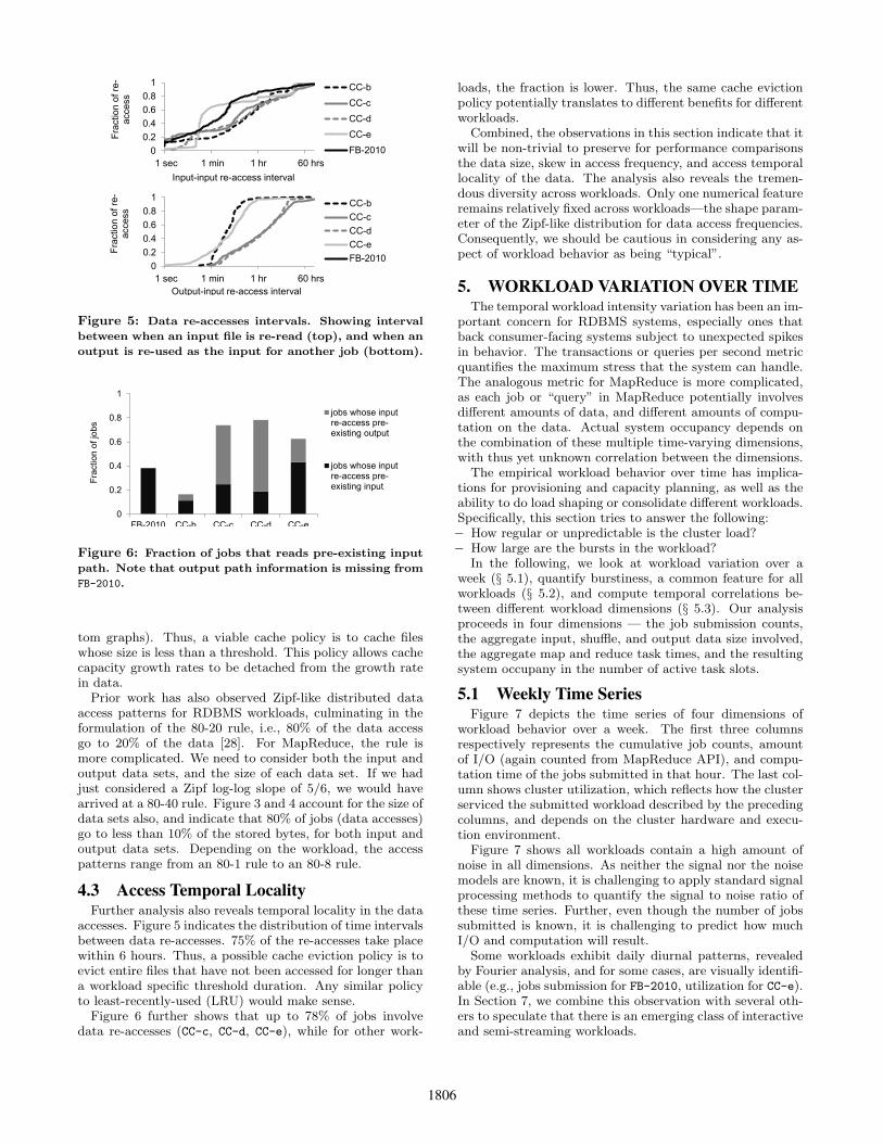
Figure 5: Data re-accesses intervals. Showing interval

between when an input file is re-read (top), and when an

output is re-used as the input for another job (bottom).

0

0.2

0.4

0.6

0.8

1

FB-2010 CC-b CC-c CC-d CC-e

Fra

ctio

n o

f jo

bs

jobs whose inputre-access pre-existing output

jobs whose inputre-access pre-existing input

Figure 6: Fraction of jobs that reads pre-existing input

path. Note that output path information is missing from

FB-2010.

tom graphs). Thus, a viable cache policy is to cache fileswhose size is less than a threshold. This policy allows cachecapacity growth rates to be detached from the growth ratein data.

Prior work has also observed Zipf-like distributed dataaccess patterns for RDBMS workloads, culminating in theformulation of the 80-20 rule, i.e., 80% of the data accessgo to 20% of the data [28]. For MapReduce, the rule ismore complicated. We need to consider both the input andoutput data sets, and the size of each data set. If we hadjust considered a Zipf log-log slope of 5/6, we would havearrived at a 80-40 rule. Figure 3 and 4 account for the size ofdata sets also, and indicate that 80% of jobs (data accesses)go to less than 10% of the stored bytes, for both input andoutput data sets. Depending on the workload, the accesspatterns range from an 80-1 rule to an 80-8 rule.

4.3 Access Temporal LocalityFurther analysis also reveals temporal locality in the data

accesses. Figure 5 indicates the distribution of time intervalsbetween data re-accesses. 75% of the re-accesses take placewithin 6 hours. Thus, a possible cache eviction policy is toevict entire files that have not been accessed for longer thana workload specific threshold duration. Any similar policyto least-recently-used (LRU) would make sense.

Figure 6 further shows that up to 78% of jobs involvedata re-accesses (CC-c, CC-d, CC-e), while for other work-

loads, the fraction is lower. Thus, the same cache evictionpolicy potentially translates to different benefits for differentworkloads.

Combined, the observations in this section indicate that itwill be non-trivial to preserve for performance comparisonsthe data size, skew in access frequency, and access temporallocality of the data. The analysis also reveals the tremen-dous diversity across workloads. Only one numerical featureremains relatively fixed across workloads—the shape param-eter of the Zipf-like distribution for data access frequencies.Consequently, we should be cautious in considering any as-pect of workload behavior as being “typical”.

5. WORKLOAD VARIATION OVER TIMEThe temporal workload intensity variation has been an im-

portant concern for RDBMS systems, especially ones thatback consumer-facing systems subject to unexpected spikesin behavior. The transactions or queries per second metricquantifies the maximum stress that the system can handle.The analogous metric for MapReduce is more complicated,as each job or “query” in MapReduce potentially involvesdifferent amounts of data, and different amounts of compu-tation on the data. Actual system occupancy depends onthe combination of these multiple time-varying dimensions,with thus yet unknown correlation between the dimensions.

The empirical workload behavior over time has implica-tions for provisioning and capacity planning, as well as theability to do load shaping or consolidate different workloads.Specifically, this section tries to answer the following:− How regular or unpredictable is the cluster load?− How large are the bursts in the workload?

In the following, we look at workload variation over aweek (§ 5.1), quantify burstiness, a common feature for allworkloads (§ 5.2), and compute temporal correlations be-tween different workload dimensions (§ 5.3). Our analysisproceeds in four dimensions — the job submission counts,the aggregate input, shuffle, and output data size involved,the aggregate map and reduce task times, and the resultingsystem occupany in the number of active task slots.

5.1 Weekly Time SeriesFigure 7 depicts the time series of four dimensions of

workload behavior over a week. The first three columnsrespectively represents the cumulative job counts, amountof I/O (again counted from MapReduce API), and compu-tation time of the jobs submitted in that hour. The last col-umn shows cluster utilization, which reflects how the clusterserviced the submitted workload described by the precedingcolumns, and depends on the cluster hardware and execu-tion environment.

Figure 7 shows all workloads contain a high amount ofnoise in all dimensions. As neither the signal nor the noisemodels are known, it is challenging to apply standard signalprocessing methods to quantify the signal to noise ratio ofthese time series. Further, even though the number of jobssubmitted is known, it is challenging to predict how muchI/O and computation will result.

Some workloads exhibit daily diurnal patterns, revealedby Fourier analysis, and for some cases, are visually identifi-able (e.g., jobs submission for FB-2010, utilization for CC-e).In Section 7, we combine this observation with several oth-ers to speculate that there is an emerging class of interactiveand semi-streaming workloads.

1806

0

100

200

0 1 2 3 4 5 6 7

Submission rate (jobs/hr)

0.0

1.0

2.0

0 1 2 3 4 5 6 7

I/O (TB/hr)

0

500

1000

1500

0 1 2 3 4 5 6 7

Compute (task-hrs/hr)

0

200

400

0 1 2 3 4 5 6 7

Utilization(slots)

Su M Tu W Th F Sa Su M Tu W Th F Sa Su M Tu W Th F Sa Su M Tu W Th F Sa

0

100

200

0 1 2 3 4 5 6 7

0

20

40

0 1 2 3 4 5 6 7

0

10000

20000

30000

0 1 2 3 4 5 6 70

2000

4000

0 1 2 3 4 5 6 7 Tu W Th F Sa Su M Tu W Th F Sa Su M Tu W Th F Sa Su M Tu W Th F Sa Su M

0

100

200

0 1 2 3 4 5 6 7

0

100

200

300

0 1 2 3 4 5 6 7

0

10000

20000

30000

0 1 2 3 4 5 6 7 Su M Tu W Th F Sa Su M Tu W Th F Sa Su M Tu W Th F Sa

0

100

200

0 1 2 3 4 5 6 7

0

100

200

300

0 1 2 3 4 5 6 7

0

10000

20000

30000

0 1 2 3 4 5 6 7 F Sa Su M Tu W Th F Sa Su M Tu W Th F Sa Su M Tu W Th

0

100

200

0 1 2 3 4 5 6 7

0

20

40

0 1 2 3 4 5 6 7

0

500

1000

1500

0 1 2 3 4 5 6 70

200

400

0 1 2 3 4 5 6 7 Tu W Th F Sa Su M Tu W Th F Sa Su M Tu W Th F Sa Su M Tu W Th F Sa Su M

0

1000

2000

3000

0 1 2 3 4 5 6 7

0

20

40

0 1 2 3 4 5 6 7

0

500

1000

1500

0 1 2 3 4 5 6 7 Su M Tu W Th F Sa Su M Tu W Th F Sa Su M Tu W Th F Sa

CC-a

CC-b

CC-c

CC-d

CC-e

FB-2009

FB-2010

0

1000

2000

3000

0 1 2 3 4 5 6 7

0

200

400

600

0 1 2 3 4 5 6 7

0

50000

100000

0 1 2 3 4 5 6 70

20000

40000

0 1 2 3 4 5 6 7 Su M Tu W Th F Sa Su M Tu W Th F Sa Su M Tu W Th F Sa Su M Tu W Th F Sa

Figure 7: Workload behavior over a week. From left to right: (1) Jobs submitted per hour. (2) Aggregate I/O

(i.e., input + shuffle + output) size of jobs submitted. (3) Aggregate map and reduce task time in task-hours of jobs

submitted. (4) Cluster utilization in average active slots. From top row to bottom, showing CC-a, CC-b, CC-c, CC-d, CC-e,

FB-2009, and FB-2010 workloads. Note that for CC-c, CC-d, and FB-2009, the utilization data is not available from the

traces. Also note that some time axes are misaligned due to short, week-long trace lengths (CC-b and CC-e), or gaps

from missing data in the trace (CC-d).

Figure 7 offers visual evidence to indicate the diversityof MapReduce workloads. There is significant variation inthe shape of the graphs for both different dimensions of thesame workloads (rows) and for the same workload dimen-sion across different workloads (columns). Consequently, forcluster management problems that involve workload varia-tion over time scales, such as load scheduling, load shifting,resource allocation, or capacity planning, approaches de-signed for one workload may be suboptimal or even counter-productive for another. As MapReduce use cases diversifyand increase in scale, it becomes vital to develop workloadmanagement techniques that can target each specific work-load.

5.2 BurstinessFigure 7 also reveals bursty submission patterns across

various dimensions. Burstiness is an often discussed prop-

erty of time-varying signals, but it is often not precisely mea-sured. One common way to attempt to measure it to use thepeak-to-average ratio. There are also domain-specific met-rics, such as for bursty packet loss on wireless links [47].Here, we extend the concept of peak-to-average ratio toquantify burstiness.

We start defining burstiness first by using the medianrather than the arithmetic mean as the measure of “aver-age”. Median is statistically robust against data outliers,i.e., extreme but rare bursts [30]. For two given workloadswith the same median load, the one with higher peaks, thatis, a higher peak-to-median ratio, is more bursty. We thenobserve that the peak-to-median ratio is the same as the100th-percentile-to-median ratio. While the median is sta-tistically robust to outliers, the 100th-percentile is not. Thisimplies that the 99th, 95th, or 90th-percentile should alsobe calculated. We extend this line of thought and compute

1807

0

0.2

0.4

0.6

0.8

1

0.01 0.1 1 10 100

Fra

ction o

f hours

Normalized task-seconds per hour

CC-a

CC-b

CC-c

CC-d

CC-e

0

0.2

0.4

0.6

0.8

1

0.01 0.1 1 10 100

Fra

ction o

f hours

Normalized task-seconds per hour

FB-2009

FB-2010

sine + 2

sine + 20

Figure 8: Workload burstiness. Showing cummulative

distribution of task-time (sum of map time and reduce

time) per hour. To allow comparison between workloads,

all values have been normalized by the median task-time

per hour for each workload. For comparison, we also

show burstiness for artificial sine submit patterns, scaled

with min-max range the same as mean (sine + 2) and

10% of mean (sine + 20).

the general nth-percentile-to-median ratio for a workload.

We can graph this vector of values, with nth−percentile

medianon

the x-axis, versus n on the y-axis. The resultant graph canbe interpreted as a cumulative distribution of arrival ratesper time unit, normalized by the median arrival rate. Thisgraph is an indication of how bursty the time series is. Amore horizontal line corresponds to a more bursty workload;a vertical line represents a workload with a constant arrivalrate.

Figure 8 graphs this metric for one of the dimensionsof our workloads. We also graph two different sinusoidalsignals to illustrate how common signals appear under thisburstiness metric. Figure 8 shows that for all workloads, thehighest and lowest submission rates are orders of magnitudefrom the median rate. This indicates a level of burstinessfar above the workloads examined by prior work, which havemore regular diurnal patterns [38, 48]. For the workloadshere, scheduling and task placement policies will be essen-tial under high load. Conversely, mechanisms for conservingenergy will be beneficial during periods of low utilization.

For the Facebook workloads, over a year, the peak-to-median-ratio dropped from 31:1 to 9:1, accompanied by moreinternal organizations adopting MapReduce. This showsthat multiplexing many workloads (workloads from manyorganizations) help decrease bustiness. However, the work-load remains bursty.

5.3 Time Series CorrelationsWe also computed the correlation between the workload

submission time series in all three dimensions. Specifically,we compute three correlation values: between the time-varying vectors jobsSubmitted(t) and dataSizeBytes(t), be-tween jobsSubmitted(t) and computeT imeTaskSeconds(t),and between dataSizeBytes(t) and computeT imeTaskSec-onds(t), where t represents time in hourly granularity, andranges over the entire trace duration.

0

0.2

0.4

0.6

0.8

1

FB-2009 FB-2010 CC-a CC-b CC-c CC-d CC-e

Corr

ela

tion

jobs - bytes

jobs - task-seconds

bytes - task-seconds

Figure 9: Correlation between different submission pat-

tern time series. Showing pair-wise correlation between

jobs per hour, (input + shuffle + output) bytes per hour,

and (map + reduce) task times per hour.

The results are in Figure 9. The average temporal correla-tion between job submit and data size is 0.21; for job submitand compute time it is 0.14; for data size and compute timeit is 0.62. The correlation between data size and computetime is by far the strongest. We can visually verify this bythe 2nd and 3rd columns for CC-e in Figure 9. This indicatesthat MapReduce workloads remain data-centric rather thancompute-centric. Also, schedulers and load balancers needto consider dimensions beyond number of active jobs.

Combined, the observations in this section mean that max-imum jobs per second is the wrong performance metric toevaluate these systems. The nature of any workload burstsdepends on the complex aggregate of data and computeneeds of active jobs at the time, as well as the scheduling,placement, and other workload management decisions thatdetermine how quickly jobs drain from the system. Anyefforts to develop a TPC-like benchmark for MapReduceshould consider a range of performance metrics, and stress-ing the system under realistic, multi-dimensional variationsin workload intensity.

6. COMPUTATION PATTERNSPrevious sections looked at data and temporal patterns

in the workload. As computation is an equally importantaspect of MapReduce, this section identifies what are thecommon computation patterns for each workload. Specifi-cally, we answer questions related to optimizing query-likeprogramming frameworks:

− What % of cluster load come from these frameworks?− What are the common uses of each framework?

We also answer questions with regard to job-level schedulingand execution planning:

− What are the common job types?− What are the size, shape, and duration of these jobs?− How frequently does each job type appear?

In traditional RDBMS, one can quantify query types bythe operator (e.g. join, select), and the cardinality of thedata processed for a particular query. Each operator canbe characterized to consume a certain amount of resourcesbased on the cardinality of the data they process. The ana-log to operators for MapReduce jobs are the map and reducesteps, and the cardinality of the data is quantified in ouranalysis by the number of bytes of data for the map input,intermediate shuffle, and reduce output stages.

1808

We consider two complementary ways of grouping MapRe-duce jobs: (1) By the job name strings submitted to MapRe-duce, which gives us insights on the use of native MapRe-duce versus query-like programatic frameworks on top ofMapReduce. For some frameworks, this analysis also revealsthe frequency of the particular query-like operators that areused (§ 6.1). (2) By the multi-dimensional job descriptionaccording to per-job data sizes, duration, and task times,which serve as a proxy to proprietary code, and indicate thesize, shape, and duration of each job type (§ 6.2).

6.1 By Job NamesJob names are user-supplied strings recorded by MapRe-

duce. Some computation frameworks built on top of MapRe-duce, such as Hive [1], Pig [3], and Oozie [2] generate the jobnames automatically. MapReduce does not currently imposeany structure on job names. To simplify analysis, we focuson the first word of job names, ignoring any capitalization,numbers, or other symbols.

Figure 10 shows the most frequent first words in job namesfor each workload, weighted by number of jobs, the amountof I/O, and task-time. The FB-2010 trace does not have thisinformation. The top figure shows that the top handful ofwords account for a dominant majority of jobs. When thesenames are weighted by I/O, Hive queries such as insert

and other data-centric jobs such as data extractors domi-nate; when weighted by task-time, the pattern is similar,unsurprising given the correlation between I/O and task-time.

Figure 10 also implies that each workload consists of onlya small number of common computation types. The rea-son is that job names are either automatically generated, orassigned by human operators using informal but commonconventions. Thus, jobs with names that begin with thesame word likely perform similar computation. The smallnumber of computation types represent targets for static oreven manual optimization. This will greatly simplify work-load management problems, such as predicting job durationor resource use, and optimizing scheduling, placement, ortask granularity.

Each workload services only a small number of MapRe-duce frameworks: Hive, Pig, Oozie, or similar layers on topof MapReduce. Figure 10 shows that for all workloads, twoframeworks account for a dominant majority of jobs. Thereis ongoing research to achieve well-behaved multiplexing be-tween different frameworks [32]. The data here suggests thatmultiplexing between two or three frameworks already cov-ers the majority of jobs in all workloads here. We believethis observation will remain valid in the future. As newframeworks develop, enterprise MapReduce users are likelyto converge on an evolving but small set of mature frame-works for business critical computations.

Figure 10 also shows that for Hive in particular, selectand insert form a large fraction of activity for several work-loads. Only the FB-2009 workload contains a large fractionof Hive queries beginning with from. Unfortunately, thisinformation is not available for Pig. Also, we see evidenceof some direct migration of established RDBMS use cases,such as etl (Extract, Transform, Load) and edw (EnterpriseData Warehouse).

This information gives us some idea with regard to goodtargets for query optimization. However, more direct infor-mation on query text at the Hive and Pig level will be even

ad

piglatin

oozie

piglatin

piglatin insert

insert

select

select

flow

flow sywr

from

insert insert

edwsequence

edwsequence

queryresult ajax

[others] [others]

twitch

snapshot

importjob select

snapshot

edw

select si

edw

tr

iteminquiry search

item

[others] esb [others]

[others]

[others]

0.0

0.2

0.4

0.6

0.8

1.0

FB-2009 CC-a CC-b CC-c CC-d CC-e

Fra

ction o

f jo

bs

from

insert

oozie

snapshot

bmdailyjob

insert insert

piglatin

metrodataextractor

tr

tr

distcp

columnset

select

select

piglatin

piglatin

select

etl

[others]

hyperlocaldataextractor

[identifier]

snapshot

[others]

parallel

insert

twitch

[identifier] ad

[others]

bmdailyjob

flow hourly

flow

[identifier2]

[others]

cascade

[others]

[others]

0.0

0.2

0.4

0.6

0.8

1.0

FB-2009 CC-a CC-b CC-c CC-d CC-e

Fra

ction o

f byt

es

from

insert

oozie

piglatin

piglatin

insert

insert

piglatin

select

tr

tr

default

etl

select

semi

[identifier]

bmdailyjob

select

columnset

[others]

stage

flow

flow

distcp

[others]

listing

snapshot

[identifier]

[others]

[others]

click

snapshot

twitch

[others]

bmdailyjob

[others]

0.0

0.2

0.4

0.6

0.8

1.0

FB-2009 CC-a CC-b CC-c CC-d CC-e

Fra

ction o

f ta

sk-t

ime

Hive Pig Oozie Others

Figure 10: The first word of job names for each work-

load, weighted by the number of jobs beginning with each

word (top), total I/O in bytes (middle), and map/reduce

task-time (bottom). For example, 44% of jobs in the

FB-2009 workload have a name beginning with “ad”, a

further 12% begin with “insert”; 27% of all I/O and

34% of total task-time comes from jobs with names that

begin with “from” (middle and bottom). The FB-2010

trace did not contain job names.

1809

more beneficial. For workflow management frameworks suchas Oozie, it will be benefitial to have UUIDs to identify jobsbelonging to the same workflow. For native MapReducejobs, it will be desirable for the job names to contain a uni-form convention of pre- and postfixes such as dates, com-putation types, steps in multi-stage processing, etc.. Ob-taining information at that level will help translate insightsfrom multi-operator RDBMS query execution planning tooptimize multi-job MapReduce workflows.

6.2 By Multi-Dimensional Job BehaviorAnother way to group jobs is by their multi-dimensional

behavior. Each job can be represented as a six-dimensionalvector described by input size, shuffle size, output size, jobduration, map task time, and reduce task time. One way togroup similarly behaving jobs is to find clusters of vectorsclose to each other in the six-dimensional space. We use astandard data clustering algorithm, k-means [9]. K-meansenables quick analysis of a large number of data points andfacilitates intuitive labeling and interpretation of cluster cen-ters [17,18, 41].

We use a standard technique to choose k, the numberof job type clusters for each workload: increment k untilthere is diminishing return in the decrease of intra-clustervariance, i.e., residual variance. Our previous work [17, 18]contains additional details of this methodology.

Table 2 summarizes our k-means analysis results. Wehave assigned labels using common terminology to describethe one or two data dimensions that separate job categorieswithin a workload. A system optimizer would use the fullnumerical descriptions of cluster centroids.

We see that jobs touching <10GB of total data make up>92% of all jobs. These jobs are capable of achieving in-teractive latency for analysts, i.e., durations of less than aminute. The dominance of these jobs counters prior assump-tions that MapReduce workloads consist of only jobs at TBscale and beyond. The observations validate research effortsto improve the scheduling time and the interactive capabilityof large-scale computation frameworks [14, 33, 39].

The dichotomy between very small and very large job hasbeen identified previously for workload management of busi-ness intelligence queries [35]. Drawing on the lessons learnedthere, poor management of a single large job potentially im-pacts performance for a large number of small jobs.

The small-big job dichotomy implies that the cluster shouldbe split into two tiers. There should be (1) a performancetier, which handles the interactive and semi-streaming com-putations and likely benefits from optimizations for interac-tive RDBMS systems, and (2) a capacity tier, which nec-essarily trades performance for efficiency in using storageand computational capacity. The capacity tier likely as-sumes batch-like semantics. One can view such a setup asanalogous to multiplexing OLTP (interactive transactional)and OLAP (potentially batch analytical) workloads. It isimportant to operate both parts of the cluster while simul-taneously achieving performance and efficiency goals.

The dominance of small jobs complicates efforts to rein instragglers [10], tasks that execute significantly slower thanother tasks in a job and delay job completion. Compar-ing the job duration and task time columns indicate thatsmall jobs contain only a handful of small tasks, sometimesa single map task and a single reduce task. Having fewcomparable tasks makes it difficult to detect stragglers, and

also blurs the definition of a straggler. If the only task ofa job runs slowly, it becomes impossible to tell whether thetask is inherently slow, or abnormally slow. The importanceof stragglers as a problem also requires re-assessment. Anystragglers will seriously hamper jobs that have a single waveof tasks. However, if it is the case that stragglers occur ran-domly with a fixed probability, fewer tasks per job meansonly a few jobs would be affected. We do not yet knowwhether stragglers occur randomly.

Interestingly, map functions in some jobs aggregate data,reduce functions in other jobs expand data, and many jobscontain data transformations in either stage. Such data ra-tios reverse the original intuition behind map functions asexpansions, i.e., “maps”, and reduction functions as aggre-gates, i.e., “reduces” [22].

Also, map-only jobs appear in all but two workloads.They form 7% to 77% of all bytes, and 4% to 42% of alltask times in their respective workloads. Some are Oozielauncher jobs and others are maintenance jobs that oper-ate on very little data. Compared with other jobs, map-only jobs benefit less from datacenter networks optimizedfor shuffle patterns [7, 8, 20, 29].

Further, FB-2010 and CC-c both contain jobs that handleroughly the same amount of data as others, but take consid-erably longer to complete versus jobs in the same workloadwith comparable data sizes. FB-2010 contains a job typethat consumes only 10s of GB of data, but requires days tocomplete (Map only transform, 3 days). These jobs haveinherently low levels of parallelism, and cannot take advan-tage of parallelism on the cluster, even if spare capacity isavailable.

Comparing the FB-2009 and FB-2010 workloads in Table 2shows that job types at Facebook changed significantly overone year. The small jobs remain, and several kinds of map-only jobs remain. However, the job profiles changed in sev-eral dimensions. Thus, for Facebook, any policy parametersneed to be periodically revisited.

Combined, the analysis once again reveals the diversityacross workloads. Even though small jobs dominate all sevenworkloads, they are “small” in different ways for each work-load. Further, the breadth of job shape, size, and durationsacross workloads indicates that microbenchmarks of a hand-ful of jobs capture only a small sliver of workload activity,and a truly representative benchmark will need to involve amuch larger range of job types.

7. TOWARDS A BIG DATA BENCHMARKIn light of the broad spectrum of industrial data presented

in this paper, it is natural to ask what implications wecan draw with regard to building a TPC-style benchmarkfor MapReduce and similar big data systems. The work-loads here are sufficient to characterize an emerging classof MapReduce workloads for interactive and semi-streaminganalysis. However, the diversity of behavior across the work-loads we analyzed means we should be careful when decidingwhich aspects of this behavior are representative enough toinclude in a benchmark. Below, we discuss some challengesassociated with building a TPC-style benchmark for MapRe-duce and other big data systems.

Data generation.

The range of data set sizes, skew in access frequency, andtemporal locality in data access all affect system perfor-

1810

# Jobs Input Shuffle Output Duration Map time Reduce time Label

CC-a 5525 51 MB 0 3.9 MB 39 sec 33 0 Small jobs194 14 GB 12 GB 10 GB 35 min 65,100 15,410 Transform31 1.2 TB 0 27 GB 2 hrs 30 min 437,615 0 Map only, huge9 273 GB 185 GB 21 MB 4 hrs 30 min 191,351 831,181 Transform and aggregate

CC-b 21210 4.6 KB 0 4.7 KB 23 sec 11 0 Small jobs1565 41 GB 10 GB 2.1 GB 4 min 15,837 12,392 Transform, small165 123 GB 43 GB 13 GB 6 min 36,265 31,389 Transform, medium31 4.7 TB 374 MB 24 MB 9 min 876,786 705 Aggregate and transform3 600 GB 1.6 GB 550 MB 6 hrs 45 min 3,092,977 230,976 Aggregate

CC-c 19975 5.7 GB 3.0 GB 200 MB 4 min 10,933 6,586 Small jobs477 1.0 TB 4.2 TB 920 GB 47 min 1,927,432 462,070 Transform, light reduce246 887 GB 57 GB 22 MB 4 hrs 14 min 569,391 158,930 Aggregate197 1.1 TB 3.7 TB 3.7 TB 53 min 1,895,403 886,347 Transform, heavy reduce105 32 GB 37 GB 2.4 GB 2 hrs 11 min 14,865,972 36,9846 Aggregate, large23 3.7 TB 562 GB 37 GB 17 hrs 9,779,062 14,989,871 Long jobs7 220 TB 18 GB 2.8 GB 5 hrs 15 min 66,839,710 758,957 Aggregate, huge

CC-d 12736 3.1 GB 753 MB 231 MB 67 sec 7,376 5,085 Small jobs214 633 GB 2.9 TB 332 GB 11 min 544,433 352,692 Expand and aggregate162 5.3 GB 6.1 TB 33 GB 23 min 2,011,911 910,673 Transform and aggregate128 1.0 TB 6.2 TB 6.7 TB 20 min 847,286 900,395 Expand and Transform43 17 GB 4.0 GB 1.7 GB 36 min 6,259,747 7,067 Aggregate

CC-e 10243 8.1 MB 0 970 KB 18 sec 15 0 Small jobs452 166 GB 180 GB 118 GB 31 min 35,606 38,194 Transform, large68 543 GB 502 GB 166 GB 2 hrs 115,077 108,745 Transform, very large20 3.0 TB 0 200 B 5 min 137,077 0 Map only summary7 6.7 TB 2.3 GB 6.7 TB 3 hrs 47 min 335,807 0 Map only transform

FB-2009 1081918 21 KB 0 871 KB 32 s 20 0 Small jobs37038 381 KB 0 1.9 GB 21 min 6,079 0 Load data, fast2070 10 KB 0 4.2 GB 1 hr 50 min 26,321 0 Load data, slow602 405 KB 0 447 GB 1 hr 10 min 66,657 0 Load data, large180 446 KB 0 1.1 TB 5 hrs 5 min 125,662 0 Load data, huge

6035 230 GB 8.8 GB 491 MB 15 min 104,338 66,760 Aggregate, fast379 1.9 TB 502 MB 2.6 GB 30 min 348,942 76,736 Aggregate and expand159 418 GB 2.5 TB 45 GB 1 hr 25 min 1,076,089 974,395 Expand and aggregate793 255 GB 788 GB 1.6 GB 35 min 384,562 338,050 Data transform19 7.6 TB 51 GB 104 KB 55 min 4,843,452 853,911 Data summary

FB-2010 1145663 6.9 MB 600 B 60 KB 1 min 48 34 Small jobs7911 50 GB 0 61 GB 8 hrs 60,664 0 Map only transform, 8 hrs779 3.6 TB 0 4.4 TB 45 min 3,081,710 0 Map only transform, 45 min670 2.1 TB 0 2.7 GB 1 hr 20 min 9,457,592 0 Map only aggregate104 35 GB 0 3.5 GB 3 days 198,436 0 Map only transform, 3 days

11491 1.5 TB 30 GB 2.2 GB 30 min 1,112,765 387,191 Aggregate1876 711 GB 2.6 TB 860 GB 2 hrs 1,618,792 2,056,439 Transform, 2 hrs454 9.0 TB 1.5 TB 1.2 TB 1 hr 1,795,682 818,344 Aggregate and transform169 2.7 TB 12 TB 260 GB 2 hrs 7 min 2,862,726 3,091,678 Expand and aggregate67 630 GB 1.2 TB 140 GB 18 hrs 1,545,220 18,144,174 Transform, 18 hrs

Table 2: Job types in each workload as identified by k-means clustering, with cluster sizes, centers, and labels. Map

and reduce time are in task-seconds, i.e., a job with 2 map tasks of 10 seconds each has map time of 20 task-seconds.

Note that the small jobs dominate all workloads.

mance. A good benchmark should stress the system withrealistic conditions in all these areas. Consequently, a bench-mark needs to pre-generate data that accurately reflects thecomplex data access patterns of real life workloads.

Processing generation.

The analysis in this paper reveals challenges in accuratelygenerating a processing stream that reflects real life work-loads. Such a processing stream needs to capture the size,shape, and sequence of jobs, as well as the aggregate clus-ter load variation over time. It is non-trivial to tease outthe dependencies between various features of the processingstream, and even harder to understand which ones we canomit for a large range of performance comparison scenarios.

Mixing MapReduce and query-like frameworks.

The heavy use of query-like frameworks on top of MapRe-duce indicates that future cluster management systems needto efficiently multiplex jobs both written in the native MapRe-duce API, and from query-like frameworks such as Hive, Pig,and HBase. Thus, a representative benchmark also needs to

include both types of processing, and multiplex them in re-alistic mixes.

Scaled-down workloads.

The sheer data size involved in the workloads means thatit is economically challenging to reproduce workload behav-ior at production scale. One can scale down workloads pro-portional to cluster size. However, there are many ways todescribe both cluster and workload size. One could normal-ize workload size parameters such as data size, number ofjobs, or the processing per data, against cluster size param-eters such as number of nodes, CPU capacity, or availablememory. It is not clear yet what would be the best way toscale down a workload.

Empirical models.

The workload behaviors we observed do not fit any well-known statistical distributions (the single exception beingZipf distribution in data access frequency). It is necessaryfor a benchmark to assume an empirical model of workloads,i.e., the workload traces are the model. This is a departure

1811

from some existing TPC-* benchmarking approaches, wherethe targeted workload are such that some simple models canbe used to generate data and the processing stream [51].

A true workload perspective.

The data in the paper indicate the shortcomings of mi-crobenchmarks that execute a small number of jobs one ata time. They are useful for diagnosing subcomponents of asystem subject to very specific processing needs. A big databenchmark should assume the perspective already reflectedin TPC-* [50], and treat a workload as a steady process-ing stream involving the superposition of many processingtypes.

Workload suites.

The workloads we analyzed exhibit a wide range of be-havior. If this diversity is preserved across more workloads,we would be compelled to accpet that no single set of be-haviors are representative. In that case, we would need toidentify as small suite of workload classes that cover a largerange of behavior. The benchmark would then consist notof a single workload, but a workload suite. Systems couldtrade optimized performance for one workload type againstmore average performance for another.

A stopgap tool.

We have developed and deployed Statistical Workload In-jector for MapReduce (https://github.com/SWIMProject-UCB/SWIM/wiki). This is a set of New BSD Licensed work-load replay tools that partially address the above challenges.The tools can pre-populate HDFS using uniform syntheticdata, scaled to the number of nodes in the cluster, and replaythe workload using synthetic MapReduce jobs. The work-load replay methodology is further discussed in [18]. TheSWIM repository already includes scaled-down versions ofthe FB-2009 and FB-2010 workloads. Cloudera has allowedus to contact the end customers directly and seek permissionto make public their traces. We hope the replay tools canact as a stop-gap while we progress towards a more thoroughbenchmark, and the workload repository can contribute toa scientific approach to designing big data systems such asMapReduce.

8. SUMMARY AND CONCLUSIONSTo summarize the analysis results, we directly answer the

questions raised in Section 2.1. The observed behavior spansa wide range across workloads, as we detail below.

1. For optimizing the underlying storage system:− Skew in data accesses frequencies range between an

80-1 and 80-8 rule.− Temporal locality exists, and 80% of data re-accesses

occur on the range of minutes to hours.

2. For workload-level provisioning and load shaping:− The cluster load is bursty and unpredictable.− Peak-to-median ratio in cluster load range from 9:1

to 260:1.

3. For job-level scheduling and execution planning:− All workloads contain a range of job types, with the

most common being small jobs.− These jobs are small in all dimensions compared

with other jobs in the same workload. They involve10s of KB to GB of data, exhibit a range of datapatterns between the map and reduce stages, andhave durations of 10s of seconds to a few minutes.

− The small jobs form over 90% of all jobs for all work-loads. The other job types appear with a wide rangeof frequencies.

4. For optimizing query-like programming frameworks:

− The cluster load that comes from these frameworksis up to 80% and at least 20%.

− The frameworks are generally used for interactivedata exploration and semi-streaming analysis. ForHive, the most commonly used operators are insertand select; from is frequently used in only oneworkload. Additional tracing at the Hive/Pig/HBaselevel is required.

5. For performance comparison between systems:− A wide variation in behavior exists between work-

loads, as the above data indicates.− There is sufficient diversity between workloads that

we should be cautious in claiming any behavior as“typical”. Additional workload studies are required.

The analysis in this paper has several repercussions: (1).MapReduce has evolved to the point where performanceclaims should be qualified with the underlying workloadassumptions, e.g., by replaying a suite of workloads. (2).System engineers should regularly re-assess design prioritiessubject to evolving use cases. Prerequisites to these effortsare workload replay tools and a public workload repository,so that engineers can share insights across different enter-prise MapReduce deployments.

Future work should seek to improve analysis and mon-itoring tools. Enterprise MapReduce monitoring tools [21]should perform workload analysis automatically, present gra-phical results in a dashboard, and ship only the anonymizedand aggregated metrics for workload comparisons offsite.Most importantly, tracing capabilities at the Hive, Pig, andHBase level should be improved. An analysis of query textat that level will reveal further insights, and expedite trans-lating RDBMS knowledge to optimize MapReduce and solvereal life problems involving large-scale data.

Improved tools will facilitate the analysis of more work-loads, over longer time periods, and for additional statistics.This improves the quality and generality of the derived de-sign insights, and contributes to the overall efforts to identifycommon behavior. The data in this paper indicate that weneed to look at a broader range of use cases before we canbuild a truly representative big data benchmark.

We invite cluster operators and the broader data manage-ment community to share additional knowledge about theirMapReduce workloads. To contribute, retain the job historylogs generated by existing Hadoop tools, run the tools athttps://github.com/SWIMProjectUCB/SWIM/wiki/Analyz-

e-historical-cluster-traces-and-synthesize-represe-

ntative-workload, and share the results.

9. ACKNOWLEDGMENTSThe authors are grateful for the feedback from our col-

leagues at UC Berkeley AMP Lab, Cloudera, Facebook,and other industrial partners. We especially appreciate theinputs from Archana Ganapathi, Anthony Joseph, DavidZats, Matei Zaharia, Jolly Chen, Todd Lipcon, Aaron T.Myers, John Wilkes, and Srikanth Kandula. This researchis supported in part by AMP Lab (https://amplab.cs.

1812

berkeley.edu/sponsors/), and the DARPA- and SRC-fund-ed MuSyC FCRP Multiscale Systems Center.

10. REFERENCES[1] Apache Hive. http://hive.apache.org/.[2] Apache Oozie(TM) Workflow Scheduler for Hadoop.

http://incubator.apache.org/oozie/.[3] Apache Pig. http://pig.apache.org/.[4] Gridmix. HADOOP-HOME/mapred/src/benchmarks/gridmix in

Hadoop 0.21.0 onwards.

[5] Hadoop World 2011 Speakers.http://www.hadoopworld.com/speakers/.

[6] Sort benchmark home page. http://sortbenchmark.org/.[7] M. Al-Fares, A. Loukissas, and A. Vahdat. A scalable,

commodity data center network architecture. InSIGCOMM, pages 63–74, 2008.

[8] M. Alizadeh et al. Data Center TCP (DCTCP). InSIGCOMM, pages 63–74, 2010.

[9] E. Alpaydin. Introduction to Machine Learning. MITPress, 2004.

[10] G. Ananthanarayanan et al. Reining in the outliers inMapReduce clusters using Mantri. In OSDI, pages 1–16,2010.

[11] G. Ananthanarayanan et al. Scarlett: coping with skewedcontent popularity in MapReduce clusters. In Eurosys,pages 287–300, 2011.

[12] G. Ananthanarayanan et al. PACMan: coordinated memorycaching for parallel jobs. In NSDI, pages 20–32, 2012.

[13] L. Bairavasundaram et al. An analysis of data corruption inthe storage stack. In FAST, pages 8:1–8:28, 2008.

[14] D. Borthakur et al. Apache Hadoop goes realtime atFacebook. In SIGMOD, pages 1071–1080, 2011.

[15] L. Breslau et al. Web caching and Zipf-like distributions:evidence and implications. In INFOCOM, pages 126–134,1999.

[16] Y. Bu et al. HaLoop: efficient iterative data processing onlarge clusters. In VLDB, pages 285–296, 2010.

[17] Y. Chen et al. Design implications for enterprise storagesystems via multi-dimensional trace analysis. In SOSP,pages 43–56, 2011.

[18] Y. Chen et al. The case for evaluating MapReduceperformance using workload suites. In MASCOTS, pages390–399, 2011.

[19] Y. Chen et al. Energy efficiency for large-scale MapReduceworkloads with significant interactive analysis. In EuroSys,pages 43–56, 2012.

[20] M. Chowdhury et al. Managing data transfers in computerclusters with orchestra. In SIGCOMM, pages 98–109, 2011.

[21] Cloudera, Inc. Cloudera Manager Datasheet.[22] J. Dean and S. Ghemawat. MapReduce: simplified data

processing on large clusters. In OSDI, pages 107–113, 2004.

[23] J. Dittrich et al. Hadoop++: making a yellow elephant runlike a cheetah (without it even noticing). In VLDB, pages515–529, 2010.

[24] EMC and IDC iView. Digital Universe.http://www.emc.com/leadership/programs/digital-universe.htm.

[25] N. Feamster and H. Balakrishnan. Detecting BGPconfiguration faults with static analysis. In NSDI, pages43–56, 2005.

[26] A. Ganapathi et al. Statistics-driven workload modeling forthe cloud. In SMDB, pages 87–92, 2010.

[27] A. F. Gates et al. Building a high-level dataflow system ontop of MapReduce: the Pig experience. In VLDB, pages1414–1425, 2009.

[28] J. Gray et al. Quickly generating billion-record syntheticdatabases. In SIGMOD, pages 243–252, 1994.

[29] A. Greenberg et al. VL2: a scalable and flexible data centernetwork. In SIGCOMM, pages 51–62, 2009.

[30] J. Hellerstein. Quantitative data cleaning for largedatabases. Technical report, United Nations EconomicCommission for Europe, 2008.

[31] H. Herodotou and S. Babu. Profiling, What-if analysis, andcost-based optimization of MapReduce programs. InVLDB, pages 1111–1122, 2011.

[32] B. Hindman et al. Mesos: A platform for fine-grainedresource sharing in the data center. In NSDI, pages 22–22,2011.

[33] M. Isard et al. Quincy: fair scheduling for distributedcomputing clusters. In SOSP, pages 261–276, 2009.

[34] E. Jahani et al. Automatic optimization for MapReduceprograms. In VLDB, pages 385–396, 2011.

[35] S. Krompass et al. Dynamic workload management for verylarge data warehouses: juggling feathers and bowling balls.In VLDB, pages 1105–1115, 2007.

[36] W. Lang and J. Patel. Energy Management for MapReduceclusters. In VLDB, pages 129–139, 2010.

[37] W. Leland et al. On the self-similar nature of Ethernettraffic. In SIGCOMM, pages 1–15, 1993.

[38] D. Meisner et al. Power management of onlinedata-intensive services. In ISCA, pages 319–330, 2011.

[39] S. Melnik et al. Dremel: interactive analysis of web-scaledatasets. In VLDB, pages 330–339, 2010.

[40] M. Mesnier et al. File classification in self-* storagesystems. In ICAC, pages 44–51, 2004.

[41] A. Mishra et al. Towards characterizing cloud backendworkloads: insights from Google compute clusters.SIGMETRICS, pages 34–41, 2010.

[42] J. C. Mogul. The case for persistent-connection HTTP. InSIGCOMM, pages 299–313, 1995.

[43] K. Morton et al. ParaTimer: A progress indicator forMapReduce DAGs. In SIGMOD, pages 507–518, 2010.

[44] J. Ousterhout et al. A trace-driven analysis of the UNIX4.2 BSD file system. In SOSP, pages 15–24, 1985.

[45] A. Pavlo et al. A comparison of approaches to large-scaledata analysis. In SIGMOD, pages 165–178, 2009.

[46] V. Paxson. End-to-end Internet packet dynamics. InSIGCOMM, pages 139–152, 1997.

[47] K. Srinivasan et al. The β-factor: measuring wireless linkburstiness. In SenSys, pages 29–42, 2008.

[48] E. Thereska, A. Donnelly, and D. Narayanan. Sierra:practical power-proportionality for data center storage. InEuroSys, pages 169–182, 2011.

[49] A. Thusoo et al. Hive: a warehousing solution over amap-reduce framework. In VLDB, pages 1626–1629, 2009.

[50] Transactional Processing Performance Council. TheTPC-W Benchmark.http://www.tpc.org/tpcw/default.asp.

[51] Transactional Processing Performance Council. TPC-*Benchmarks. http://www.tpc.org/.

1813