Integrating Physics-Based Modeling With Machine Learning ...
34
Integrating Physics-Based Modeling With Machine Learning: A Survey JARED WILLARD ∗ and XIAOWEI JIA ∗ , University of Minnesota SHAOMING XU, University of Minnesota MICHAEL STEINBACH, University of Minnesota VIPIN KUMAR, University of Minnesota There is a growing consensus that solutions to complex science and engineering problems require novel methodologies that are able to integrate traditional physics-based modeling approaches with state-of-the-art machine learning (ML) techniques. This paper provides a structured overview of such techniques. Application areas for which these approaches have been applied are summarized, then classes of methodologies used to construct physics-guided ML models and hybrid physics-ML frameworks are described. We then provide a taxonomy of these existing techniques, which uncovers knowledge gaps and potential crossovers of methods between disciplines that can serve as ideas for future research. Additional Key Words and Phrases: physics-guided, neural networks, deep learning, physics-informed, theory- guided, hybrid, knowledge integration ACM Reference Format: Jared Willard, Xiaowei Jia, Shaoming Xu, Michael Steinbach, and Vipin Kumar. 2020. Integrating Physics-Based Modeling With Machine Learning: A Survey. 1, 1 (July 2020), 34 pages. https://doi.org/10.1145/1122445.1122456 1 INTRODUCTION Machine learning (ML) models, which have already found tremendous success in commercial applications, are beginning to play an important role in advancing scientific discovery in domains traditionally dominated by mechanistic (e.g. first principle) models [22, 112, 117, 126, 127, 138, 214, 261]. The use of ML models is particularly promising in scientific problems involving processes that are not completely understood, or where it is computationally infeasible to run mechanistic models at desired resolutions in space and time. However, the application of even the state-of-the-art black box ML models has often met with limited success in scientific domains due to their large data requirements, inability to produce physically consistent results, and their lack of generalizability to out-of-sample scenarios [126]. Given that neither an ML-only nor a scientific knowledge-only approach can be considered sufficient for complex scientific and engineering applications, the research community is beginning to explore the continuum between mechanistic and ML models, where both scientific knowledge and data are integrated in a synergistic manner [2, 14, 126, 204]. This work was supported by NSF grant #1934721 and by DARPA award W911NF-18-1-0027. ∗ Both authors contributed equally to this research. Authors’ addresses: Jared Willard, [email protected]; Xiaowei Jia, [email protected], University of Minnesota, Minneapo- lis, Minnesota, 55455; Shaoming Xu, [email protected], University of Minnesota, Minneapolis, Minnesota, 55455; Michael Steinbach, [email protected], University of Minnesota, Minneapolis, Minnesota, 55455; Vipin Kumar, [email protected], University of Minnesota, Minneapolis, Minnesota, 55455. Permission to make digital or hard copies of all or part of this work for personal or classroom use is granted without fee provided that copies are not made or distributed for profit or commercial advantage and that copies bear this notice and the full citation on the first page. Copyrights for components of this work owned by others than ACM must be honored. Abstracting with credit is permitted. To copy otherwise, or republish, to post on servers or to redistribute to lists, requires prior specific permission and/or a fee. Request permissions from [email protected]. © 2020 Association for Computing Machinery. XXXX-XXXX/2020/7-ART $15.00 https://doi.org/10.1145/1122445.1122456 , Vol. 1, No. 1, Article . Publication date: July 2020. arXiv:2003.04919v4 [physics.comp-ph] 14 Jul 2020
Transcript of Integrating Physics-Based Modeling With Machine Learning ...
Integrating Physics-Based Modeling With MachineLearning: A Survey
JARED WILLARD∗ and XIAOWEI JIA∗, University of MinnesotaSHAOMING XU, University of MinnesotaMICHAEL STEINBACH, University of MinnesotaVIPIN KUMAR, University of Minnesota
There is a growing consensus that solutions to complex science and engineering problems require novelmethodologies that are able to integrate traditional physics-based modeling approaches with state-of-the-artmachine learning (ML) techniques. This paper provides a structured overview of such techniques. Applicationareas for which these approaches have been applied are summarized, then classes of methodologies used toconstruct physics-guided ML models and hybrid physics-ML frameworks are described. We then provide ataxonomy of these existing techniques, which uncovers knowledge gaps and potential crossovers of methodsbetween disciplines that can serve as ideas for future research.
Additional Key Words and Phrases: physics-guided, neural networks, deep learning, physics-informed, theory-guided, hybrid, knowledge integration
ACM Reference Format:JaredWillard, Xiaowei Jia, Shaoming Xu, Michael Steinbach, and Vipin Kumar. 2020. Integrating Physics-BasedModelingWith Machine Learning: A Survey. 1, 1 (July 2020), 34 pages. https://doi.org/10.1145/1122445.1122456
1 INTRODUCTIONMachine learning (ML) models, which have already found tremendous success in commercialapplications, are beginning to play an important role in advancing scientific discovery in domainstraditionally dominated by mechanistic (e.g. first principle) models [22, 112, 117, 126, 127, 138, 214,261]. The use of ML models is particularly promising in scientific problems involving processes thatare not completely understood, or where it is computationally infeasible to run mechanistic modelsat desired resolutions in space and time. However, the application of even the state-of-the-art blackbox ML models has often met with limited success in scientific domains due to their large datarequirements, inability to produce physically consistent results, and their lack of generalizabilityto out-of-sample scenarios [126]. Given that neither an ML-only nor a scientific knowledge-onlyapproach can be considered sufficient for complex scientific and engineering applications, theresearch community is beginning to explore the continuum between mechanistic and ML models,where both scientific knowledge and data are integrated in a synergistic manner [2, 14, 126, 204].
This work was supported by NSF grant #1934721 and by DARPA award W911NF-18-1-0027.∗Both authors contributed equally to this research.
Authors’ addresses: Jared Willard, [email protected]; Xiaowei Jia, [email protected], University of Minnesota, Minneapo-lis, Minnesota, 55455; Shaoming Xu, [email protected], University of Minnesota, Minneapolis, Minnesota, 55455; MichaelSteinbach, [email protected], University of Minnesota, Minneapolis, Minnesota, 55455; Vipin Kumar, [email protected],University of Minnesota, Minneapolis, Minnesota, 55455.
Permission to make digital or hard copies of all or part of this work for personal or classroom use is granted without feeprovided that copies are not made or distributed for profit or commercial advantage and that copies bear this notice andthe full citation on the first page. Copyrights for components of this work owned by others than ACM must be honored.Abstracting with credit is permitted. To copy otherwise, or republish, to post on servers or to redistribute to lists, requiresprior specific permission and/or a fee. Request permissions from [email protected].© 2020 Association for Computing Machinery.XXXX-XXXX/2020/7-ART $15.00https://doi.org/10.1145/1122445.1122456
, Vol. 1, No. 1, Article . Publication date: July 2020.
arX
iv:2
003.
0491
9v4
[ph
ysic
s.co
mp-
ph]
14
Jul 2
020

2 Jared Willard, Xiaowei Jia, Shaoming Xu, Michael Steinbach, and Vipin Kumar
This paradigm is fundamentally different from mainstream practices in the ML community formaking use of domain-specific knowledge, albeit in subservient roles, e.g., feature engineering orpost-processing. In contrast to these practices that can only work with simpler forms of heuristicsand constraints, this survey is focused on those approaches that explore a deeper coupling of MLmethods with scientific knowledge.
Even though the idea of integrating scientific principles andMLmodels has picked up momentumjust in the last few years [126], there is already a vast amount of work on this topic. This workis being pursued in diverse disciplines (e.g., earth systems [214], climate science [75, 135, 186],turbulence modeling [28, 179, 273], material discovery [40, 202, 226], quantum chemistry [222, 228],biological sciences [285], and hydrology [275]), and it is being performed in the context of diverseobjectives specific to these applications. Early results in isolated and relatively simple scenarioshave been promising, and the expectations are rising for this paradigm to accelerate scientificdiscovery and help address some of the biggest challenges that are facing humanity in terms ofclimate [75], health [259], and food security [118].The goal of this survey is to bring these exciting developments to the ML community, to make
them aware of the progress that has been made, and the gaps and opportunities that exist foradvancing research in this promising direction. We hope that this survey will also be valuable forscientists who are interested in exploring the use of ML to enhance modeling in their respectivedisciplines. Please note that work on this topic has been referred to by other names, such as"physics-guided ML," "physics-informed ML," or "physics-aware AI," although it covers manyscientific disciplines. In this survey, we also use the terms "physics-guided" or "physics," whichshould be more generally or interpreted as science or scientific knowledge.The focus of this survey is on approaches that integrate mechanistic modeling with ML, using
primarily ideas from physics and other scientific disciplines. This distinguishes our survey fromother works that focus on more general knowledge integration into machine learning [1, 256] andother works covering physics integration into ML in specific domains (e.g., cyber-physical systems[204], chemistry [184]). This survey creates a novel taxonomy specific to science-based knowledgeand covers a wide array of both methodologies and categories.We organize the paper as follows. Section 2 describes different objectives that are being used
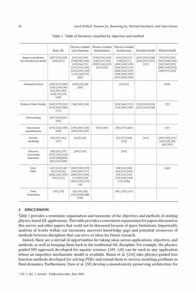
through combinations of scientific knowledge and machine learning. Section 3 discusses novel MLmethods and architectures that researchers are developing to achieve these objectives. Section 4discusses opportunities for future research, and Section 5 contains concluding remarks. Table 1categorizes the work surveyed in this paper by objectives and approaches.
2 OBJECTIVES OF PHYSICS-ML INTEGRATIONThis section provides a brief overview of a diverse set of objectives where deep couplings of ML andscientific modeling paradigms are being pursued in the context of various applications. Though weenumerate these distinct categories in the following subsections, there are numerous cross-cuttingthemes. One is the use of ML as a surrogate model where the goal is to accurately reproducethe behavior of a mechanistic model at substantially reduced computational cost. Reduction incomputational cost is a known characteristic of ML in comparison to the often high cost ofnumerical simulations, and ML-based surrogate models are relevant for many objectives. Also,though uncertainty quantification is its own subsection, it is relevant for most of the other objectives.
2.1 Improving predictions beyond that of state-of-the-art physical modelsFirst-principles models are used extensively in a wide range of engineering and environmentalapplications. Even though these models are based on known physical laws, in most cases, they are
, Vol. 1, No. 1, Article . Publication date: July 2020.
Integrating Physics-Based Modeling With Machine Learning: A Survey 3
necessarily approximations of reality due to incomplete knowledge of certain processes, whichintroduces bias. In addition, they often contain a large number of parameters whose values must beestimated with the help of limited observed data, degrading their performance further, especiallydue to heterogeneity in the underlying processes in both space and time. The limitations of physics-based models cut across discipline boundaries and are well known in the scientific community (e.g.,see Gupta et al. [103] in the context of hydrology).ML models have been shown to outperform physics-based models in many disciplines (e.g.,
materials science [130, 220, 263], applied physics [15, 116], aquatic sciences [120], atmosphericscience [185], biomedical science [245], computational biology [3]). A major reason for this successis that ML models (e.g., neural networks), given enough data, can find structure and patternsin problems where complexity prohibits the explicit programming of a system’s exact physicalnature. Given this ability to automatically extract complex relationships from data, ML modelsappear promising for scientific problems with physical processes that are not fully understood byresearchers, but for which data of adequate quality and quantity is available. However, the black-boxapplication of ML has met with limited success in scientific domains due to a number of reasons[120, 126]: (i) while state-of-the-art ML models are capable of capturing complex spatiotemporalrelationships, they require far too much labeled data for training, which is rarely available in realapplication settings, (ii) ML models often produce scientifically inconsistent results; and (iii) MLmodels can only capture relationships in the available training data, and thus cannot generalize toout-of-sample scenarios (i.e., those not represented in the training data).The key objective here is to combine elements of physics-based modeling with state-of-the-art
ML models to leverage their complementary strengths. Such integrated physics-ML models areexpected to better capture the dynamics of scientific systems and advance the understanding ofunderlying physical processes. Early attempts for combining ML with physics-based modeling inseveral applications (e.g., modeling the lake phosphorus concentration [109] and lake temperaturedynamics [120, 128, 213]) have already demonstrated its potential for providing better predictionaccuracy with a much smaller number of samples as well as generalizability in out-of-samplescenarios.
2.2 DownscalingComplex first principle models are capable of capturing physical reality more precisely thansimpler models, as they often involve more diverse components that account for a greater numberof processes at finer spatial or temporal resolution. However, given the computation cost andmodeling complexity, many models are run at a resolution that is coarser than what is requiredto precisely capture underlying physical processes. For example, cloud-resolving models (CRM)need to run at sub-kilometer horizontal resolution to be able to effectively represent boundary-layer eddies and low clouds, which are crucial for the modeling of Earth’s energy balance and thecloud–radiation feedback [212]. However, it is not feasible to run global climate models at such fineresolutions even with the most powerful commuters expected to be available in the near future.
Downscaling techniques have been widely used as a solution to capture physical variables thatneed to be modeled at a finer resolution. In general, the downscaling techniques can be divided intotwo categories: statistical downscaling and dynamical downscaling. Statistical downscaling refersto the use of empirical models to predict finer-resolution variables from coarser-resolution variables.Such a mapping across different resolutions can involve complex non-linear relationships thatcannot be precisely modeled by simple empirical models. Recently, artificial neural networks haveshown a lot of promise for this problem, given their ability to model non-linear relationships [232,254]. In contrast, dynamical downscaling makes use of high-resolution regional simulations todynamically simulate relevant physical processes at regional or local scales of interest. Due to
, Vol. 1, No. 1, Article . Publication date: July 2020.
4 Jared Willard, Xiaowei Jia, Shaoming Xu, Michael Steinbach, and Vipin Kumar
the substantial time cost of running such complex models, there is an increasing interest in usingML models as surrogate models (a model approximating simulation-driven input–output data) topredict target variables at a higher resolution [90, 237].
Although the state-of-the-art MLmethods can be used in both statistical and dynamical downscal-ing, it remains a challenge to ensure that the learned ML component is consistent with establishedphysical laws and can improve the overall simulation performance.
2.3 ParameterizationComplex physics-based models (e.g., for simulating phenomena in climate, weather, turbulencemodeling, astrophysics) often use an approach known as parameterization to account for missingphysics. In parameterization (note that this term has a different meaning when used in mathematicsand geometry), specific complex dynamical processes are replaced by simplified physical approxi-mations whose associated parameter values are estimated from data, often through a procedurereferred to parameter calibration. The failure to correctly identify parameter values can make themodel less robust, and errors that result from imperfect parameterization can also feed into othercomponents of the entire physics-based model and deteriorate the modeling of important physicalprocesses. Hence, there is great interest in using ML models to learn new parameterizations directlyfrom observations and/or high-resolution model simulation. Already, ML-based parameterizationshave shown success in geology [43, 95] and atmospheric science [32, 33, 90, 186]. A major bene-fit of ML-based parameterizations is the reduction of computation time compared to traditionalphysics-based simulations. In chemistry, Hansen et al. [108] find that parameterizations of atomicenergy using ML take seconds compared to multiple days for more standard quantum-calculationcalculations, and Behler et al. [20] find that neural networks can vastly improve the efficiency offinding potential energy surfaces of molecules.
Most of the existing work uses standard black box ML models for parameterization, but there isan increasing interest in integrating physics in the ML models [23], as it has the potential to makethem more robust and generalizable to unseen scenarios as well as reduce the number of trainingsamples needed for training.Note that both parameterization and downscaling described in Section 2.2 are used to replace
components of larger models. To avoid confusion, we distinctly use downscaling to relate toresolutions (e.g., resolving certain physical processes to higher resolutions) and use parameterizationfor creating simplified parameterized approximations of complex dynamical processes.
2.4 Reduced-Order ModelsReduced-Order Models (ROMs) are computationally inexpensive representations of more complexmodels. Usually, constructing ROMs involves dimensionality reduction that attempts to capturethe most important dynamical characteristics of often large, high-fidelity simulations and modelsof physical systems (e.g., in fluid dynamics [145]). This can also be viewed as a controlled lossof accuracy. A common way to do this is to project the governing equations of a system onto alinear subspace of the original state space using a method such as principal components analysisor dynamic mode decomposition [201]. However, limiting the dynamics to a lower-dimensionalsubspace inherently limits the accuracy of any ROM.
ML is beginning to assist in constructing ROMs for increased accuracy and reduced computationalcost in several ways. One approach is to build an ML-based surrogate model for full-order models[46], where the ML model can be considered a ROM. Other ways include building an ML-basedsurrogate model of an already built ROM by another dimensionality reduction method [273] orbuilding an ML model to mimic the dimensionality reduction mapping from a full-order model to areduced-order model [179]. ML and ROMs can also be combined by using the ML model to learn
, Vol. 1, No. 1, Article . Publication date: July 2020.
Integrating Physics-Based Modeling With Machine Learning: A Survey 5
the residual between a ROM and observational data [257]. ML models have the potential to greatlyaugment the capabilities of ROMs because of their typically quick forward execution speed andability to leverage data to model high dimensional phenomena.One area of recent focus of ML-based ROMs is in approximating the dominant modes of the
Koopman (or composition) operator, as a method of dimensionality reduction. The Koopmanoperator is an infinite-dimension linear operator that encodes the temporal evolution of the systemstate through nonlinear dynamics [36]. This allows linear analysismethods to be applied to nonlinearsystems and enables the inference of properties of dynamical systems that are too complex toexpress using traditional analysis techniques. Applications span many disciplines, including fluiddynamics [233], oceanography [93], molecular dynamics [267], and many others. Though dynamicmode decomposition [178] is the most common technique for approximating the Koopman operator,many recent approaches have been made to approximate Koopman operator embeddings withdeep learning models that outperform existing methods [150, 163, 171, 180, 188, 190, 244, 262, 286].Adding physics-based knowledge to the learning of the Koopman operator has the potential toaugment generalizability and interpretability, which current ML methods in this area tend to lack[190].ROMs often lack robustness with respect to parameter changes within the systems they are
representing [5], or are not cost-effective enoughwhen trying to predict complex dynamical systems(e.g., multiscale in space and time). Thus, incorporating principles from physics-based models couldpotentially reduce the search space to enable more robust training of ROMs, and also allow themodel to be trained with less data in many scenarios.
2.5 Inverse ModelingThe forward modeling of a physical system uses the physical parameters of the system (e.g., mass,temperature, charge, physical dimensions or structure) to predict the next state of the system or itseffects (outputs). In contrast, inverse modeling uses the (possibly noisy) output of a system to inferthe intrinsic physical parameters. Inverse problems often stand out as important in physics-basedmodeling communities because they can potentially shed light on valuable information that cannotbe observed directly. One example is the use of x-ray images from a CT scan to create a 3D imagereflecting the structure of part of a person’s body. This can be viewed as a computer vision problem,where, given many training datasets of x-ray scans of the body at different capture angles, a modelcan be trained to inversely reconstruct textures and 3D shapes of different organs or other areas ofinterest. Allowing for better reconstruction while reducing scan time could potentially increasepatient satisfaction and reduce overall medical costs.
Often, the solution of an inverse problem can be computationally expensive due to the potentiallymillions of forward model evaluations needed for estimator evaluation or characterization ofposterior distributions of physical parameters [84]. ML-based surrogate models (in addition toother methods such as reduced-order models) are becoming a realistic choice since they canmodel high-dimensional phenomena with lots of data and execute much faster than most physicalsimulations.Inverse problems are traditionally solved using regularized regression techniques. Data-driven
methods have seen success in inverse problems in remote sensing of surface properties [59],photonics [197], and medical imaging [161], among many others. Recently, novel algorithms usingdeep learning and neural networks have been applied to inverse problems.While still in their infancy,these techniques exhibit strong performance for applications such as computerized tomography[47, 174], seismic processing [253], or various sparse data problems.
There is also increasing interest in the inverse design of materials using ML, where desired targetproperties of materials are used as input to the model to identify atomic structures that exhibit such
, Vol. 1, No. 1, Article . Publication date: July 2020.
6 Jared Willard, Xiaowei Jia, Shaoming Xu, Michael Steinbach, and Vipin Kumar
properties [137, 151, 202, 226]. Physics-based constraints and stopping conditions based on materialproperties can be used to guide the optimization process [151]. These constraints and similarphysics-guided techniques have the potential to alleviate noted challenges in inverse modeling,particularly in scenarios with a small sample size and a paucity of ground-truth labels [127]. Theintegration of prior physical knowledge is common in current approaches to the inverse problem,and its integration into ML-based inverse models has the potential to improve data efficiency andincrease its ability to solve ill-posed inverse problems.
2.6 Forward Solving Partial Differential EquationsIn many physical systems, governing equations are known, but direct numerical solutions of partialdifferential equations (PDEs) using common methods, such as the Finite Elements Method or theFinite Difference Method [80], are prohibitively expensive. In such cases, traditional methods arenot ideal or sometimes even possible. A common technique is to use an ML model as a surrogatefor the solution to reduce computation time [65, 140]. In particular, NN solvers can reduce thehigh computational demands of traditional numerical methods into a single forward-pass of a NN.Notably, solutions obtained via NNs are also naturally differentiable and have a closed analytic formthat can be transferred to any subsequent calculations, a feature not found inmore traditional solvingmethods [140]. Especially with the recent advancement of computational power, neural networksmodels have shown success in approximating solutions across different kinds of physics-basedPDEs [9, 131, 215], including the difficult quantum many-body problem [42] and many-electronSchrodinger equation [107]. As a step further, deep neural networks models have shown successin approximating solutions across high dimensional physics-based PDEs previously consideredunsuitable for approximation by ML [106, 235]. However, slow convergence in training, limitedapplicability to many complex systems, and reduced accuracy due to unawareness of physical lawscan prove problematic.
2.7 Discovering Governing EquationsWhen the governing equations of a dynamical system are known explicitly, they allow for morerobust forecasting, control, and the opportunity for analysis of system stability and bifurcationsthrough increased interpretability [217]. Furthermore, if the learned mathematical model accuratelydescribes the processes governing the observed data, it therefore can generalize to data outsideof the training domain. However, in many disciplines (e.g., neuroscience, cell biology, finance,epidemiology) dynamical systems have no formal analytic descriptions. Often in these cases, datais abundant, but the underlying governing equations remain elusive. In this section, we discussequation discovery systems that do not assume the structure of the desired equation (as in Section2.6), but rather explore a space a large space of possibly nonlinear mathematical terms.Advances in ML for the discovery of these governing equations has become an active research
area with rich potential to integrate principles from applied mathematics and physics with modernML methods. Early works on the data-driven discovery of physical laws relied on heuristics andexpert guidance and were focused on rediscovering known, non-differential, laws in differentscientific disciplines from artificial data [92, 143, 144, 149]. This was later expanded to includereal-world data and differential equations in ecological applications [72]. Recently, general androbust data-driven discovery of potentially unknown governing equations has been pioneered by[30, 227], where they apply symbolic regression to differences between computed derivatives andanalytic derivatives to determine underlying dynamical systems. More recently, works have usedsparse regression built on a dictionary of functions and partial derivatives to construct governingequations [37, 200, 216]. Lagergren et al. [141] expand on this by using ANNs to construct thedictionary of functions. These sparse identification techniques are based on the principle of Occam’s
, Vol. 1, No. 1, Article . Publication date: July 2020.
Integrating Physics-Based Modeling With Machine Learning: A Survey 7
Razor, where the goal is that only a few equation terms be used to describe any given nonlinearsystem.
2.8 Data GenerationData generation approaches are useful for creating virtual simulations of scientific data underspecific conditions. For example, these techniques can be used to generate potential chemicalcompounds with desired characteristics (e.g., serving as catalysts or having a specific crystalstructure). Traditional physics-based approaches for generating data often rely on running physicalsimulations or conducting physical experiments, which tend to be very time consuming. Also,these approaches are restricted by what can be produced by physics-based models. Hence, these isan increasing interest in generative ML approaches that learn data distributions in unsupervisedsettings and thus have the potential to generate novel data beyond what could be produced bytraditional approaches.
Generative ML models have found tremendous success in areas such as speech recognition andgeneration [187], image generation [63], and natural language processing [100]. These models havebeen at the forefront of unsupervised learning in recent years, mostly due to their efficiency inunderstanding unlabeled data. The idea behind generativemodels is to capture the inner probabilisticdistribution in order to generate similar data. With the recent advances in deep learning, newgenerative models, such as the generative adversarial network (GAN) and variational autoencoder(VAE), have been developed. These models have shown much better performance in learning non-linear relationships to extract representative latent embeddings from observation data. Hence thedata generated from the latent embeddings are more similar to true data distribution. In particular,the adversarial component of GAN consists of a two-part framework of a generative network anddiscriminative network, where the generative network’s objective is to generate fake data to foolthe discriminative network, while the discriminative network attempts to determine true data fromfake data.In the scientific domain, GANs can generate data like the data generated by the physics-based
models. Using GANs often incurs certain benefits, including reduced computation time and abetter reproduction of complex phenomenon, given the ability of GANs to represent nonlinearrelationships. For example, Farimani et al. [78] have shown that Conditional Generative AdversarialNetworks (cGAN) can be trained to simulate heat conduction and fluid flow purely based onobservations without using knowledge of the underlying governing equations. Such approachesthat use generative models have been shown to significantly accelerate the process of generatingnew data samples.However, a well-known issue of GANs is that they incur dramatically high sample complexity.
Therefore, a growing area of research is to engineer GANs that can leverage prior knowledgeof physics in terms of physical laws and invariance properties. For example, GAN-based modelsfor simulating turbulent flows can be further improved by incorporating physical constraints,e.g., conservation laws [288] and energy spectrum [269], in the loss function. Cang et al. [40]also imposed a physics-based morphology constraint on a VAE-based generative model used forsimulating artificial material samples. The physics-based constraint forces the generated artificialsamples to have the same morphology distribution as the authentic ones and thus greatly reducesthe large material design space.
2.9 UncertaintyQuantificationUncertainty quantification (UQ) is of great importance in many areas of computational science(e.g., climate modeling [64], fluid flow [55], systems engineering [195], among many others). Atits core, UQ requires an accurate characterization of the entire distribution p(y |x), where y is the
, Vol. 1, No. 1, Article . Publication date: July 2020.
8 Jared Willard, Xiaowei Jia, Shaoming Xu, Michael Steinbach, and Vipin Kumar
response and x is the covariate of interest, rather than just making a point prediction y = f (x).This makes it possible to characterize all quantiles and skews in the distribution, which allows foranalysis such as examining how close predictions are to being unacceptable, or sensitivity analysisof input features.Applying UQ tasks to physics-based models using traditional methods such as Monte Carlo
(MC) is usually infeasible due to the thousands or millions of forward model evaluations needed toobtain convergent statistics. In the physics-based modeling community, a common technique is toperform model reduction (described in Section 2.4) or create an ML surrogate model, in order toincrease model evaluation speed since ML models often execute much faster [87, 170, 250]. With asimilar goal, the ML community has often employed Gaussian Processes as the main technique forquantifying uncertainty in simulating physical processes [26, 211], but neither Gaussian Processesnor reduced models scale well to higher dimensions or larger datasets (Gaussian Processes scale asO(N 3) with N data points).Consequently, there is an effort to fit deep learning models, which have exhibited countless
successes across disciplines, as a surrogate for numerical simulations in order to achieve fastermodel evaluations for UQ that have greater scalability than Gaussian Processes [250]. However,since artificial neural networks do not have UQ naturally built into them, variations have beendeveloped. One such modification uses a probabilistic drop-out strategy in which neurons areperiodically "turned off" as a type of Bayesian approximation to estimate uncertainty [86]. Thereare also Bayesian variants of neural networks that consist of distributions of weights and biases[164, 296, 300], but these suffer from high computation times and high dependence on reliablepriors. Another method uses an ensemble of neural networks to create a distribution from whichuncertainty is quantified [142].The integration of prior physics knowledge into ML for UQ has the potential to allow for a
better characterization of uncertainty. For example, ML surrogate models run the risk of producingphysically inconsistent predictions, and incorporating elements of physics could help with thisissue. Also, note that the reduced data needs of ML due to constraints for adherence to knownphysical laws could alleviate some of the high computational cost of Bayesian neural networks forUQ.
3 PHYSICS-ML METHODSGiven the diversity of forms in which scientific knowledge is represented in different disciplinesand applications, a diverse set of methodologies are needed to integrate physical principles intoML models. This section creates a taxonomy of five classes of methodologies to merge principles ofphysics-based modeling with ML; (i) physics-guided loss function, (ii) physics-guided initialization,(iii) physics-guided design of architecture, (iv) residual modeling, and (v) hybrid physics-ML models.
3.1 Physics-Guided Loss FunctionScientific problems often exhibit a high degree of complexity due to relationships between manyphysical variables varying across space and time at different scales. Standard ML models can fail tocapture such relationships directly from data, especially when provided with limited observationdata. This is one reason for their failure to generalize to scenarios not encountered in trainingdata. Researchers are beginning to incorporate physical knowledge into loss functions to help MLmodels capture generalizable dynamic patterns consistent with established physical laws.One of the most common techniques to make ML models consistent with physical laws is to
incorporate physical constraints into the loss function of ML models as follows [126],
Loss = LossTRN(Ytrue,Ypred) + λR(W ) + γLossPHY(Ypred) (1)
, Vol. 1, No. 1, Article . Publication date: July 2020.
Integrating Physics-Based Modeling With Machine Learning: A Survey 9
where the training loss LossTRN measures a supervised error (e.g., RMSE or cross-entropy) betweentrue labels Ytrue and predicted labels Ypred, and λ is a hyper-parameter to control the weight ofmodel complexity loss R(W ). These first two terms are the standard loss of ML models. The additionof physics-based loss LossPHY aims to ensure consistency with physical laws and it is weighted bya hyper-parameter γ .Steering ML predictions towards physically consistent outputs has numerous benefits. First,
the computation of physics-based loss LossPHY requires no observation data and thus optimiz-ing LossPHY allows including unlabeled data in training. Second, the regularization by physicalconstraints can reduce the possible search space of parameters. This provides possibility to learnwith less labeled data while also ensuring the consistency with physical laws during optimization.Third, ML models which follow desired physical properties are more likely to be generalizable toout-of-sample scenarios, and thus become acceptable for use by domain scientists and stakeholdersin physical science applications. Loss function terms corresponding to physical constraints are ap-plicable across many different types of ML frameworks and objectives. In the following paragraphs,we demonstrate the use of physics-based loss functions for different objectives described in Section2.
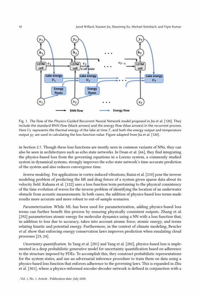
Improving predictions. In the context of complex natural systems, incorporation of physics-basedloss has shown great success in improving prediction ability of ML models. In the context oflake temperature modeling, Karpatne et al. [128] includes an additional physics-based penaltythat ensures that predictions of denser water predictions are at lower depths than predictions ofless dense water, a known monotonic relationship. Jia et al. [119] and Read et al. [213] furtherextended this work to capture even more complex and general physical relationships that happenon a temporal scale. Specifically, they use a physics-based penalty for energy conservation inthe loss function to ensure the lake thermal energy gain across time is consistent with the netthermodynamic fluxes in and out of the lake. A diagram of this model is shown in Figure 1. Notethat the recurrent structure contains additional nodes (shown in blue) to represent physical variable(lake energy, etc) that are computed using purely physics-based equations. These are needed toincorporate energy conservation in the loss function. Similar structure can be used to model otherphysical laws such as mass conservation.
Solving and Discovering PDEs and Governing Equations. Another strand of work that involves lossfunction alterations is solving PDEs for dynamical systems modeling, in which adherence to thegoverning equations is enforced in the loss function. In Raissi et al. [208], this concept is developedand shown to create data-efficient spatiotemporal function approximators to both solve and findparameters of basic PDEs like Burgers Equation or Schrodinger Equation. Going beyond a simplefeed-forward network, Zhu et al. [301] propose an encoder-decoder for predicting transient PDEswith governing PDE constraints. Geneva et al. [89] extended this approach to deep auto-regressivedense encoder-decoders with a Bayesian framework using stochastic weight averaging to quantifyuncertainty.
Qualitative mathematical properties of dynamical systems modeling have also shown promise ininforming loss functions for improved prediction beyond that of the physics model. Erichson et al.[74] penalize autoencoders based on physically meaningful stability measures in dynamical systemsfor improved prediction of fluid flow and sea surface temperature. They showed an improvedmapping of past states to future states in time in both modeling scenarios in addition to improvedgeneralizability to new data.
Physics-based loss function terms have also been used in the discovery of governing equations.Loiseau et al. [155] uses constrained least squares [96] to incorporate energy-preserving nonlineari-ties or to enforce symmetries in the identified equations to the equation learning process described
, Vol. 1, No. 1, Article . Publication date: July 2020.
10 Jared Willard, Xiaowei Jia, Shaoming Xu, Michael Steinbach, and Vipin Kumar
Fig. 1. The flow of the Physics-Guided Recurrent Neural Network model proposed in Jia et al. [120]. Theyinclude the standard RNN flow (black arrows) and the energy flow (blue arrows) in the recurrent process.HereUT represents the thermal energy of the lake at time T , and both the energy output and temperatureoutput yT are used in calculating the loss function value. Figure adapted from Jia et al. [120].
in Section 2.7. Though these loss functions are mostly seen in common variants of NNs, they canalso be seen in architectures such as echo state networks. In Doan et al. [66], they find integratingthe physics-based loss from the governing equations in a Lorenz system, a commonly studiedsystem in dynamical systems, strongly improves the echo state network’s time-accurate predictionof the system and also reduces convergence time.
Inverse modeling. For applications in vortex induced vibrations, Raissi et al. [210] pose the inversemodeling problem of predicting the lift and drag forces of a system given sparse data about itsvelocity field. Kahana et al. [122] uses a loss function term pertaining to the physical consistencyof the time evolution of waves for the inverse problem of identifying the location of an underwaterobstacle from acoustic measurements. In both cases, the addition of physics-based loss terms maderesults more accurate and more robust to out-of-sample scenarios.
Parameterization. While ML has been used for parameterization, adding physics-based lossterms can further benefit this process by ensuring physically consistent outputs. Zhang et al.[292] parameterizes atomic energy for molecular dynamics using a NN with a loss function that,in addition to loss due to accuracy, takes into account atomic force, atomic energy, and termsrelating kinetic and potential energy. Furthermore, in the context of climate modeling, Beucleret al. show that enforcing energy conservation laws improves prediction when emulating cloudprocesses [23, 24].
Uncertainty quantification. In Yang et al. [281] and Yang et al. [282], physics-based loss is imple-mented in a deep probabilistic generative model for uncertainty quantification based on adherenceto the structure imposed by PDEs. To accomplish this, they construct probabilistic representationsfor the system states, and use an adversarial inference procedure to train them on data using aphysics-based loss function that enforces adherence to the governing laws. This is expanded in Zhuet al. [301], where a physics-informed encoder-decoder network is defined in conjunction with a
, Vol. 1, No. 1, Article . Publication date: July 2020.
Integrating Physics-Based Modeling With Machine Learning: A Survey 11
conditional flow-based generative model for similar purposes. A similar loss function modification isperformed in other works [89, 129, 278], but for the purpose of solving high dimensional stochasticPDEs with uncertainty propagation. In these cases, physics-guided constraints provide effectiveregularization for training deep generative models to serve as surrogates of physical systems wherethe cost of acquiring data is high and the data sets are small [282].Another direction for encoding physics knowledge into ML UQ applications is to create a
physics-guided Bayesian NN. This is explored in Yang et al. [277], where they use a Bayesian NN,which naturally encodes uncertainty, as a surrogate for a PDE solution. Additionally, they adda PDE constraint for the governing laws of the system to serve as a prior for the Bayesian net,allowing for more accurate predictions in situations with significant noise due to the physics-basedregularization.
Generative models. In recent years, GANs have been used to efficiently generate solutions toPDEs and there is interest in using physics knowledge to improve them. Work by Yang et al. [279]shows GANs with loss functions based on PDEs can be used to solve stochastic elliptic PDEs in up to30 dimensions. In a similar vein, Wu et al. [268] showed that physics-based loss functions in GANscan lower the amount of data and training time needed to converge on solutions of turbulencePDEs, while Shan et al. [231] saw similar results in the generation of microstructures satisfyingcertain physical properties in computational materials science.
3.2 Physics-Guided InitializationSince many ML models require an initial choice of model parameters before training, researchershave explored different ways to physically inform a model starting state. For example, in NNs,weights are often initialized according to a random distribution prior to training. Poor initializationcan cause models to anchor in local minima, which is especially true for deep neural networks.However, if physical or other contextual knowledge can be used to help inform the initializationof the weights, model training can be accelerated or improved [120]. One way to inform theinitialization to assist in model training and escaping local minima is to use an ML techniqueknown as transfer learning. In transfer learning, a model can be pre-trained on a related task priorto being fine-tuned with limited training data to fit the desired task. The pre-trained model servesas an informed initial state that ideally is closer to the desired parameters for the desired taskthan random initialization. One way to harness physics-based modeling knowledge is to use thephysics-based model’s simulated data to pre-train the ML model, which also alleviates data paucityissues. This is similar to the common application of pre-training in computer vision, where CNNsare often pre-trained with very large image datasets before being fine-tuned on images from thetask at hand [243].
Jia et al. use this strategy in the context of modeling lake temperature dynamics [119, 120]. Theypre-train their Physics-Guided Recurrent Neural Network (PGRNN) models for lake temperaturemodeling on simulated data generated from a physics-based model and fine tune the NN withlittle observed data. They showed that pre-training, even using data from a physical model withan incorrect set of parameters, can still significantly reduce the training data needed for a qualitymodel. In addition, Read et al. [213] demonstrated that such models are able to generalize better tounseen scenarios than pure physics-based models.Another application can be seen in computer vision in robotics, where images from robotics
simulations have been shown to be sufficient without any real-world data for the task of objectlocalization [248], while reducing data requirements by a factor of 50 for object grasping [31]. Then,in autonomous vehicle training, Shah et al. [230] showed that pre-training the driving algorithm ina simulator built on a video game physics engine can drastically lessen data needs. More generally,
, Vol. 1, No. 1, Article . Publication date: July 2020.
12 Jared Willard, Xiaowei Jia, Shaoming Xu, Michael Steinbach, and Vipin Kumar
we see that simulation pre-training of applications allows for significantly less expensive datacollection than is possible with physical robots.Another significant application of physics-guided initialization is in computational biophysics,
where high computational cost of molecular dynamics simulations limits the number of mutantmolecules that can be investigated from a given baseline molecule. Sultan et al. [239] showed thatthe molecular dynamics of a mutant protein can be estimated by training a variational autoencoderon the simulation of the protein from which the target protein mutated, allowing for surrogatemodels to offset the high cost of simulations. This method promises to be able to quickly samplerelated molecular systems to enable probing of the variation in large complex molecular structures,an otherwise very computationally expensive task. In a similar vein, in the context of predictingprotein structures, Hurtado et al. [114] shows that a deep NN can be pre-trained on a large databaseof already-known protein structures to enhance performance.
Physics-guided model initialization has also been employed in chemical process modeling [158,159, 276]. Yan et al. [276] uses Gaussian process regression for process modeling that has beentransferred and adapted from a similar task. To adapt the transferred model, they use scale-biascorrecting functions optimized throughmaximum likelihood estimation of parameters. Furthermore,Gaussian process models come equipped with uncertainty quantification which is also informedthrough initialization. A similar transfer and adapt approach is seen in Lu et al. [158], but for anensemble of NNs transferred from related tasks. In both of the previous studies, the similarity metricsused to find similar systems are defined by considering various common process characteristicsand behaviors.
3.3 Physics-Guided Design of ArchitectureAlthough the physics-based loss and initialization in the previous sections helps constrain the searchspace of ML models during training, the ML architecture is often still a black box. In particular, theydo not use any architectural properties to implicitly encode physical consistency or other desiredphysical properties. A recent research direction has been to construct new ML architectures thatcan make use of the specific characteristics of the problem being solved. . Though this section isfocused largely on neural network architecture, we also include subsections on multi-task learningand structures of Gaussian processes. The modular and flexible nature of NNs in particular makethem prime candidates for architecture modification. For example, domain knowledge can used tospecify node connections that capture physics-based dependencies among variables. Furthermore,incorporating physics-based guidance into architecture has the added bonus of also making thepreviously black box algorithm more interpretable, a desirable but typically missing feature of MLmodels used in physical modeling. In the following paragraphs, we discuss several contexts inwhich physics-guided ML architectures have been used.
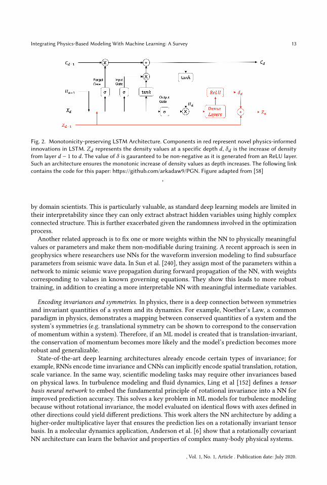
Intermediate Physical Variables. One way to embed known physical principles into NN design isto ascribe physical meaning for certain neurons in the NN. It is also possible to declare physicallyrelevant variables explicitly. In lake temperature modeling, Daw et al. [58] incorporate a physicalintermediate variable as part of a monotonicity-preserving structure in the LSTM architecture asshown in Figure 2. This model produces physically consistent predictions in addition to appending adropout layer to quantify uncertainty. In Muralidlar et al. [182], a similar approach is taken to insertphysics-constrained variables as the intermediate variables in the convolutional neural network(CNN) architecture and achieve significant improvement over state-of-the-art physics-based modelson the problem of predicting drag force on particle suspensions in moving fluids.
An additional benefit of adding physically relevant intermediate variables in an ML architectureis that they can help extract physically meaningful hidden representation that can be interpreted
, Vol. 1, No. 1, Article . Publication date: July 2020.
Integrating Physics-Based Modeling With Machine Learning: A Survey 13
Fig. 2. Monotonicity-preserving LSTM Architecture. Components in red represent novel physics-informedinnovations in LSTM. Zd represents the density values at a specific depth d , δd is the increase of densityfrom layer d − 1 to d . The value of δ is gauranteed to be non-negative as it is generated from an ReLU layer.Such an architecture ensures the monotonic increase of density values as depth increases. The following linkcontains the code for this paper: https://github.com/arkadaw9/PGN. Figure adapted from [58]
,
by domain scientists. This is particularly valuable, as standard deep learning models are limited intheir interpretability since they can only extract abstract hidden variables using highly complexconnected structure. This is further exacerbated given the randomness involved in the optimizationprocess.
Another related approach is to fix one or more weights within the NN to physically meaningfulvalues or parameters and make them non-modifiable during training. A recent approach is seen ingeophysics where researchers use NNs for the waveform inversion modeling to find subsurfaceparameters from seismic wave data. In Sun et al. [240], they assign most of the parameters within anetwork to mimic seismic wave propagation during forward propagation of the NN, with weightscorresponding to values in known governing equations. They show this leads to more robusttraining, in addition to creating a more interpretable NN with meaningful intermediate variables.
Encoding invariances and symmetries. In physics, there is a deep connection between symmetriesand invariant quantities of a system and its dynamics. For example, Noether’s Law, a commonparadigm in physics, demonstrates a mapping between conserved quantities of a system and thesystem’s symmetries (e.g. translational symmetry can be shown to correspond to the conservationof momentum within a system). Therefore, if an ML model is created that is translation-invariant,the conservation of momentum becomes more likely and the model’s prediction becomes morerobust and generalizable.State-of-the-art deep learning architectures already encode certain types of invariance; for
example, RNNs encode time invariance and CNNs can implicitly encode spatial translation, rotation,scale variance. In the same way, scientific modeling tasks may require other invariances basedon physical laws. In turbulence modeling and fluid dynamics, Ling et al [152] defines a tensorbasis neural network to embed the fundamental principle of rotational invariance into a NN forimproved prediction accuracy. This solves a key problem in ML models for turbulence modelingbecause without rotational invariance, the model evaluated on identical flows with axes defined inother directions could yield different predictions. This work alters the NN architecture by adding ahigher-order multiplicative layer that ensures the prediction lies on a rotationally invariant tensorbasis. In a molecular dynamics application, Anderson et al. [6] show that a rotationally covariantNN architecture can learn the behavior and properties of complex many-body physical systems.
, Vol. 1, No. 1, Article . Publication date: July 2020.
14 Jared Willard, Xiaowei Jia, Shaoming Xu, Michael Steinbach, and Vipin Kumar
In a general setting, Wang et al. [260] show how spatiotemporal models can be made moregeneralizable by incorporating symmetries into deep NNs. More specifically, they demonstratedthe encoding of translational symmetries, rotational symmetries, scale invariances, and uniformmotion into NNs using customized convolutional layers in CNNs that enforce desired invarianceproperties. They also provided theoretical guarantees of invariance properties across the differentdesigns and showed additional to significant increases in generalization performance.
Incorporating symmetries, by informing the structure of the solution space, also has the potentialto reduce the search space of an ML algorithm. This is important in the application of discoveringgoverning equations, where the space of mathematical terms and operators is exponentially large.Though in its infancy, physics-informed architectures for discovering governing equations arebeginning to be investigated by researchers. In Section 2.7, symbolic regression is mentioned asan approach that has shown success. However, given the massive search space of mathematicaloperators, analytic functions, constants, and state variables, the problem can quickly become NP-hard. Udrescu et al. [251] designs a recursive multidimensional version of symbolic regression thatuses a NN in conjunction with techniques from physics to narrow the search space. Their idea is touse NNs to discover hidden signs of "simplicity", such as symmetry or separability in the trainingdata, which enables breaking the massive search space into smaller ones with fewer variables to bedetermined.
In the context of molecular dynamics applications, a number of researchers [21, 292] have useda NN per individual atom to calculate each atom’s contribution to the total energy. Then, to ensurethe energy invariance with respect to the possibility of interchanging two atoms, the structure ofeach NN and the values of each network’s weight parameters are constrained to be identical foratoms of the same element. More recently, novel deep learning architectures have been proposed forfundamental invariances in chemistry. Schutt et al. [228] proposes continuous-filter convolutional(cfconv) layers for CNNs to allow for modeling objects with arbitrary positions such as atoms inmolecules, in contrast to objects described by Cartesian-gridded data such as images. Furthermore,their architecture uses atom-wise layers that incorporate inter-atomic distances that enabled themodel to respect quantum-chemical constraints such as rotationally invariant energy predictionsas well as energy-conserving force predictions. Furthermore, Zhang et al. [293] propose an end-to-end modeling framework that preserves all natural symmetries of a molecular system using anembedding procedure that maps the input to symmetry-preserving components. This is furtherexpanded for 3D point clouds in the "Tensor field networks" proposed by Thomas et al. [246], wherethey use continuous convolution layers on point cloud data, and also constrain the network filtersto be the product of a learnable radial function and a spherical harmonic that make them rotation-and translation-equivariant. As we can see, because molecular dynamics often ascribes importanceto different important geometric properties of molecules (e.g. rotation), network architecturesdealing with invariances can be effective for improving performance and robustness of ML models.Architecture modifications incorporating symmetry are also seen extensively in dynamical
systems research involving differential equations. In a pioneering work by Ruthotto et al [218],three variations of CNNs are proposed for solving PDEs. Each variation uses mathematical theoriesto guide the design of the CNN based on fundamental properties of the PDEs. Multiple types ofmodifications are made, including adding symmetry layers to guarantee the stability expressedby the PDEs and layers that convert inputs to kinematic eigenvalues that satisfy certain physicalproperties. They define a parabolic CNN inspired by anisotropic filtering, a hyperbolic CNN basedon Hamiltonian systems, and a second order hyperbolic CNN. Hyperbolic CNNs were found topreserve the energy in the system as intended, which set them apart from parabolic CNNs thatsmooth the output data, reducing the energy.
, Vol. 1, No. 1, Article . Publication date: July 2020.
Integrating Physics-Based Modeling With Machine Learning: A Survey 15
A recent direction also relating to conserved or invariant quantities is the incorporation ofthe Hamiltonian operator into NNs [54, 98, 249, 299]. The Hamiltonian operator in physics is theprimary tool for modeling the time evolution of systemswith conserved quantities, but until recentlythe formalism had not been integrated with NNs. Greydanus et al. [98] design a NN architecture thatnaturally learns and respects energy conservation and other invariance laws in simple mass-springor pendulum systems. They accomplish this through predicting the Hamiltonian of the system andre-integrating instead of predicting the state of physical systems themselves. This is taken a stepfurther in Toth et al. [249], where they show that not only can NNs learn the Hamiltonian, but alsothe abstract phase space (assumed to be known in Greydanus et al. [98]) to more effectively modelexpressive densities in similar physical systems and also extend more generally to other problemsin physics. Recently, the Hamiltonian-parameterized NNs above have also been expanded into NNarchitectures that perform additional differential equation-based integration steps based on thederivatives approximated by the Hamiltonian network [51].
Encoding other domain-specific physical knowledge. Various other domain-specific physical infor-mation can be encoded into architecture that doesn’t exactly correspond to known invariancesbut provides meaningful structure to the optimization process depending on the task at hand. Thiscan take place in many ways, including using domain-informed convolutions for CNNs, additionaldomain-informed discriminators in GANs, or structures informed by the physical characteristics ofthe problem. For example, Sadoughi et al. [221] prepend a CNN with a Fast Fourier Transform layerand a physics-guided convolution layer based on known physical information pertaining to faultdetection of rolling element bearings. A similar approach is used in Sturmfels et al. [238], but theadded beginning layer instead serves to segment different areas of the brain for domain guidancein neuroimaging tasks. In the context of generative models, Xie et al. [274] introduce tempoGAN,which augments a general adversarial network with an additional discriminator network along withadditional loss function terms that preserve temporal coherence in the generation of physics-basedsimulations of fluid flow. This type of approach, though found mostly in NN models, has beenextended to non-NN models in Baseman et al. [17], where they introduce a physics-guided MarkovRandom Field that encodes spatial and physical properties of computer memory devices into thecorresponding probabilistic dependencies.
A number of advances in encoding physical knowledge have beenmade in the context of quantumchemistry and molecular dynamics. In computational quantum chemistry, Pfau et al. [196] developthe paradigm of spin-based neural-network quantum states by defining a custom NN architectureto map electron states to the atom’s wave function, which characterizes its atomic state. Keyarchitecture components are intermediate layers in the NN to take the mean of the activationfunctions from each electron stream, and a final layer which applies a quantum spin-dependentlinear transformation, weights the desired outputs as the solution wave function, and enforcesany boundary conditions. In molecular kinetics, reduced order modeling frameworks are used forapproximating the Koopman operator [171, 262]. Mardt et al. [171] describe a dual NN architecturethat transforms the molecular configurations found at given time delays (e.g. t and t + τ ) to Markovstates along simulation trajectories to perform nonlinear dimensionality reduction. They show thisoutperforms state-of-the-art existing methods and also remains interpretable due to the mappingto realistic physical states. A similar approach is seen in [262], where they take a similar time-delayapproach to improve over state-of-the-art but instead use autoencoders, which allows for theaddition of a decoding step that can predict configurations in the original coordinate space fromlatent space points. This encoder-decoder architecture is further expanded on by Otto et al. [188],where they go beyond linear reconstruction using Koopman modes in the decoder step to an
, Vol. 1, No. 1, Article . Publication date: July 2020.

16 Jared Willard, Xiaowei Jia, Shaoming Xu, Michael Steinbach, and Vipin Kumar
architecture that does nonlinear reconstruction in order to learn ever lower dimensional Koopmansubspaces.Fan et al. [77] define new architectures to solve the inverse problem of electrical impedance
tomography, where the goal is to determine the electrical conductivity distribution of an unknownmedium from electrical measurements along its boundary. They define new NN layers based on alinear approximation of both the forward and inverse maps relying on the nonstandard form of thewavelet decomposition [25].
Architecture modifications are also seen in dynamical systems research encoding principlesfrom differential equations. Chen et al. [48] develops a continuous depth NN based on the ResidualNetwork [110] for solving ordinary differential equations. They change the traditionally discretizedneuron layer depths into continuous equivalents such that hidden states can be parameterizedby differential equations in continuous time. This allows for increased computational efficiencydue to the simplification of the backpropagation step of training, and also creates a more scalablenormalizing flow, an architectural component for solving PDEs. This is done by by parameterizingthe derivative of the hidden states of the NN as opposed to the states themselves. Then, in a similarapplication, Chang et al. [44] uses principles from the stability properties of differential equations indynamical systems modeling to guide the design of the gating mechanism and activation functionsin an RNN.
Currently, human experts have manually developed the majority of domain knowledge-encodedemployed architectures, which can be a time-intensive and error-prone process. Because of this,there is increasing interest in automated neural architecture search methods [13, 73, 115]. A youngbut promising direction in ML architecture design is to embed prior physical knowledge into neuralarchitecture searches. Ba et al. [12] adds physically meaningful input nodes and physical operationsbetween nodes to the neural architecture search space to enable the search algorithm to discovermore ideal physics-guided ML architectures.
Auxiliary Task in Multi-Task Learning. Domain knowledge can be incorporated into ML architec-ture as auxiliary tasks in a multi-task learning framework. Multi-task learning allows for multiplelearning tasks to be solved at the same time, ideally while exploiting commonalities and differencesacross tasks. This can result in improved learning efficiency and predictions for one or more of thetasks. Therefore, another way to implement physics-based learning constraints is to use an auxiliarytask in a multi-task learning framework. Here, an example of an auxiliary task in a multi-taskframework might be related to ensuring physically consistent solutions in addition to accuratepredictions. The promise of such an approach was demonstrated for a computer vision task byintegrating auxiliary information (e.g. pose estimation) for facial landmark detection [297]. In thisparadigm, a task-constrained loss function can be formulated to allow errors of related tasks to beback-propagated jointly to improve model generalization. Early work in a computational chemistryapplication showed that a NN could be trained to predict energy by constructing a loss functionthat had penalties for both inaccuracy and inaccurate energy derivatives with respect to time asdetermined by the surrounding energy force field [199]. In particle physics, De Oliveira et al. [62]uses an additional task for the discriminator network in a generative adversarial network (GAN) tosatisfy certain properties of particle interaction for the production of jet images of particle energy.
Physics-guided Gaussian process regression. Gaussian process regression (GPR) [265] is a nonpara-metric, Bayesian approach to regression that is increasingly being used in ML applications. GPRhas several benefits, including working well on small amounts of data and enabling uncertaintymeasurements on predictions. In GPR, first a Gaussian process prior must be assumed in the formof a mean function and a matrix-valued kernel or covariance function. One way to incorporatephysical knowledge in GPR is to encode differential equations into the kernel [242]. This is a key
, Vol. 1, No. 1, Article . Publication date: July 2020.
Integrating Physics-Based Modeling With Machine Learning: A Survey 17
feature in Latent Force Models, which attempt to use equations in the physical model of the systemto inform the learning from data [4, 160]. Alvarez et al. [4] draws inspiration from similar applica-tions in bioinformatics [88, 146], which showed an increase in predictive ability in computationalbiology, motion capture, and geostatistics datasets. More recently, Glielmo et al. [94] propose avectorial GPR that encodes physical knowledge in the matrix-valued kernel function. They showrotation and reflection symmetry of the interatomic force between atoms can be encoded in theGaussian process with specific invariance-preserving covariant kernels. Furthermore, Raissi etal. [206] show that the covariance function can explicitly encode the underlying physical lawsexpressed by differential equations in order to solve PDEs and learn with smaller datasets.
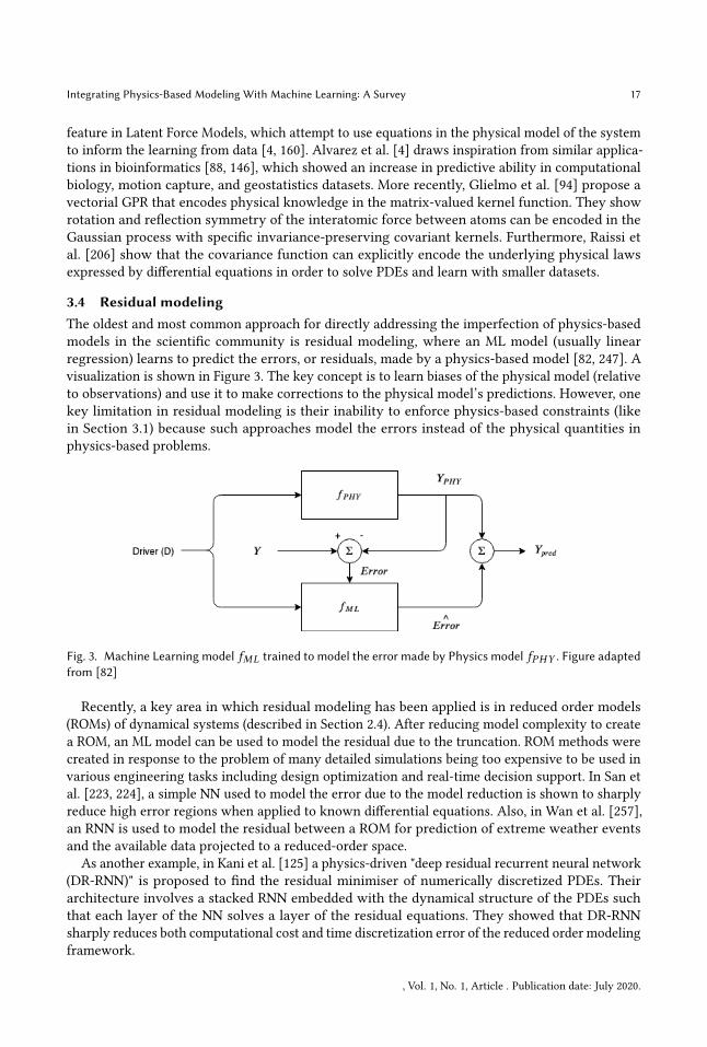
3.4 Residual modelingThe oldest and most common approach for directly addressing the imperfection of physics-basedmodels in the scientific community is residual modeling, where an ML model (usually linearregression) learns to predict the errors, or residuals, made by a physics-based model [82, 247]. Avisualization is shown in Figure 3. The key concept is to learn biases of the physical model (relativeto observations) and use it to make corrections to the physical model’s predictions. However, onekey limitation in residual modeling is their inability to enforce physics-based constraints (likein Section 3.1) because such approaches model the errors instead of the physical quantities inphysics-based problems.
Fig. 3. Machine Learning model fML trained to model the error made by Physics model fPHY . Figure adaptedfrom [82]
Recently, a key area in which residual modeling has been applied is in reduced order models(ROMs) of dynamical systems (described in Section 2.4). After reducing model complexity to createa ROM, an ML model can be used to model the residual due to the truncation. ROM methods werecreated in response to the problem of many detailed simulations being too expensive to be used invarious engineering tasks including design optimization and real-time decision support. In San etal. [223, 224], a simple NN used to model the error due to the model reduction is shown to sharplyreduce high error regions when applied to known differential equations. Also, in Wan et al. [257],an RNN is used to model the residual between a ROM for prediction of extreme weather eventsand the available data projected to a reduced-order space.
As another example, in Kani et al. [125] a physics-driven "deep residual recurrent neural network(DR-RNN)" is proposed to find the residual minimiser of numerically discretized PDEs. Theirarchitecture involves a stacked RNN embedded with the dynamical structure of the PDEs suchthat each layer of the NN solves a layer of the residual equations. They showed that DR-RNNsharply reduces both computational cost and time discretization error of the reduced order modelingframework.
, Vol. 1, No. 1, Article . Publication date: July 2020.
18 Jared Willard, Xiaowei Jia, Shaoming Xu, Michael Steinbach, and Vipin Kumar
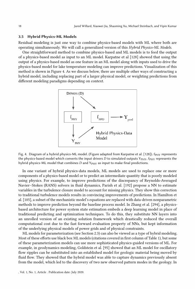
3.5 Hybrid Physics-ML ModelsResidual modeling is just one way to combine physics-based models with ML where both areoperating simultaneously. We will call a generalized version of this Hybrid Physics-ML Models.One straightforward method to combine physics-based and ML models is to feed the output
of a physics-based model as input to an ML model. Karpatne et al [128] showed that using theoutput of a physics-based model as one feature in an ML model along with inputs used to drive thephysics-based model for lake temperature modeling can improve predictions. Visualization of thismethod is shown in Figure 4. As we discuss below, there are multiple other ways of constructing ahybrid model, including replacing part of a larger physical model, or weighting predictions fromdifferent modeling paradigms depending on context.
Fig. 4. Diagram of a hybrid physics-ML model. (Figure adapted from Karpatne et al. [128]). fPHY representsthe physics-based model which converts the input drivers D to simulated outputs YPHY, fPHY represents thehybrid physics-ML model that combines D and YPHY as input to make final predictions.
In one variant of hybrid physics-data models, ML models are used to replace one or morecomponents of a physics-based model or to predict an intermediate quantity that is poorly modeledusing physics. For example, to improve predictions of the discrepancy of Reynolds-AveragedNavier–Stokes (RANS) solvers in fluid dynamics, Parish et al. [192] propose a NN to estimatevariables in the turbulence closure model to account for missing physics. They show this correctionto traditional turbulence models results in convincing improvements of predictions. In Hamilton etal. [105], a subset of the mechanistic model’s equations are replaced with data-driven nonparametricmethods to improve prediction beyond the baseline process model. In Zhang et al. [294], a physics-based architecture for power system state estimation embeds a deep learning model in place oftraditional predicting and optimization techniques. To do this, they substitute NN layers intoan unrolled version of an existing solution framework which drastically reduced the overallcomputational cost due to the fast forward evaluation property of NNs, but kept informationof the underlying physical models of power grids and of physical constraints.
ML models for parameterization (see Section 2.3) can also be viewed as a type of hybrid modeling.Most of these efforts use black boxMLmodels (citations covered in first column of Table 1), but someof these parameterization models can use more sophisticated physics-guided versions of ML. Forexample, in geodynamics modeling, Goldstein et al. [95] showed that an ML model for oscillatoryflow ripples can be substituted into an established model for geologic material being moved byfluid flow. They showed that the hybrid model was able to capture dynamics previously absentfrom the model, which led to the discovery of two new observed pattern modes in the geology. In
, Vol. 1, No. 1, Article . Publication date: July 2020.
Integrating Physics-Based Modeling With Machine Learning: A Survey 19
chemical physics, Manzhos et al. [169] first showed that NNs could be used to represent componentfunctions within high dimensional model representations (HDMR) of energy potentials. They showthis improves the quality of the final representation and reduces the cost of the fits of componentfunctions for HDMR traditionally done with explicit equations. Furthermore, the generality of thehybrid framework allows the HDMR to be constructed in a black box, molecule-independent way.In another class of hybrid frameworks, the overall prediction is a combination of predictions
from a physical model and an ML model, where the weights depend on prediction circumstance.For example, long-range interactions (e.g. gravity) can often be more easily modeled by classicalphysics equations than more stochastic short-range interactions (quantum mechanics) that arebetter modeled using data-driven alternatives. Hybrid frameworks like this have been used toadaptively combineML predictions for short-range processes and physicsmodel predictions for long-range processes for applications in chemical reactivity [284] and seismic activity prediction [191].Estimator quality at a given time and location can also be used to determine whether a predictioncomes from the physical model or the ML model, which was shown in Chen et al. [50] for airpollution estimation and in Vlachas et al. [255] for dynamical system forecasting more generally. Inthe context of solving PDEs, Malek et al [166] showcases a hybrid NN and traditional optimizationtechnique to find the closed analytical form of the solution of a PDE. In this hybrid solver, thereexist two terms, a term described by the NN and a term described by traditional optimizationtechniques.Moreover, in inverse modeling, there is a growing use of hybrid models that first use physics-
based models to perform the direct inversion, then use deep learning models to further refinethe inverse model’s predictions. Multiple works have shown an effective application for this incomputed tomography (CT) reconstructions [38, 121]. Another common technique in inversemodeling of images (e.g. medical imaging, particle physics imaging), is the use of CNNs as deepimage priors [252]. To simultaneously exploit data and prior knowledge, Senouf et al. [229] embeda CNN that serves as the image prior for a physics-based forward model for MRIs.
, Vol. 1, No. 1, Article . Publication date: July 2020.
20 Jared Willard, Xiaowei Jia, Shaoming Xu, Michael Steinbach, and Vipin Kumar
Table 1. Table of literature classified by objective and method
Basic MLPhysics-GuidedLoss Function
Physics-GuidedInitialization
Physics-GuidedArchitecture Residual Model Hybrid Model
Improve predictionbeyond physical model
[287] [35] [102][104] [271]
[247] [4] [199][139][128] [160][183] [66] [74][119] [153] [182][213] [295] [109][113] [165] [79]
[285]
[158] [276] [162][248] [31] [230][239] [114] [119]
[213] [276]
[152] [56] [17][238] [6] [11]
[183] [182] [193][196] [221] [113][260] [154] [293][232] [292] [289][291] [246] [228]
[247] [275] [258][223] [257] [271]
[153]
[95] [99] [222][105] [128] [236][50] [156] [191][284] [294] [255][280] [97] [165]
Parameterization [198] [157] [203][135] [169] [95][43] [90] [186][212] [29] [33]
[189]
[292] [23] [24][285]
[21] [23] [294]
Reduced Order Models [244] [179] [101][273] [225] [286]
[173]
[188] [10] [148] [125] [262] [171][74] [188] [190]
[125] [223] [224][257] [101] [190]
[57]
Downscaling [237] [254] [81][232]
Uncertaintyquantification
[275] [142] [250][283]
[270] [281] [266][282] [301] [89]
[276] [162] [58] [277] [266] [67]
Inversemodeling
[59] [47] [161][197]
[210] [122] [27] [77] [240][132]
[111] [192] [105] [121][241] [39] [38][68] [229]
DiscoverGoverningEquations
[30] [227] [37][167] [168] [216][123] [200][205][52] [141] [290]
[207] [155] [251]
SolvePDEs
[147] [65] [140][9] [215] [42]
[264] [106] [235][107] [131]
[209] [234] [279][281] [60] [177][208] [231] [301][71] [89] [129][268] [194] [176]
[16]
[48] [218] [44][60] [172] [235][19] [51] [131][76] [278] [194][176] [206]
[166]
DataGeneration
[187] [78] [62] [40] [28][133] [268] [288]
[298]
[49] [274] [231]
4 DISCUSSIONTable 1 provides a systematic organization and taxonomy of the objectives and methods of existingphysics-basedML applications. This table provides a convenient organization for papers discussed inthis survey and other papers that could not be discussed because of space limitations. Importantly,analysis of works within our taxonomy uncovers knowledge gaps and potential crossovers ofmethods between disciplines that can serve as ideas for future research.
Indeed, there are a myriad of opportunities for taking ideas across applications, objectives, andmethods, as well as bringing them back to the traditional ML discipline. For example, the physics-guided NN approach developed for aquatic sciences [109, 120] can be used in any applicationwhere an imperfect mechanistic model is available. Raissi et al. [210] take physics-guided lossfunction methods developed for solving PDEs and extend them to inverse modeling problems influid dynamics. Furthermore, Daw et al. [58] develop a monotonicity-preserving architecture for
, Vol. 1, No. 1, Article . Publication date: July 2020.
Integrating Physics-Based Modeling With Machine Learning: A Survey 21
lake temperature based on previous work done using loss function terms and a hybrid physics-MLarchitecture [128].
Note that some techniques for incorporating physical principles into ML models can be appliedto a wide range of objectives. For example, the physics-guided loss function spans nearly all therows of Table 1. Methods also have the potential for overlap, where, for example, physics-guidedloss functions, physics-guided architecture, and physics-guided initialization could all be applied toan ML model used in a hybrid framework.From Table 1, it is easy to see that several boxes in the Table 1 are rather sparse or entirely
empty, many of which represent opportunities for future work. For example, ML models forparameterization are increasingly being used in domains such as climate science and weatherforecasting [135], all of which can benefit from the integration of physical principles. Furthermore,principles from super-resolution frameworks, originally developed in the context of computervision applications, are beginning to be applied to downscaling to create higher resolution climatepredictions [254]. However, most of these do not incorporate physics (e.g., through additionalloss function terms or an informed design of architecture). The fact that nearly all of the othermethods (columns) except for hybrid modeling are applicable to this task shows that there istremendous scope for new exploration, where research pursued in these columns in the contextof other objectives can be applied for this objective. We also see a lot of opportunities for newresearch on physics-guided initialization, where, for example, pre-training an ML algorithm forinverse modeling or parameterization on simulation data related to the desired task could improveperformance or lessen data needs.We note that many boxes in Table 1 may not make sense for the pairing of an objective with
a method. In particular, residual modeling (which is one of the oldest approaches for integratingphysical models with statistical/machine learning models) cannot be naturally used for manyof the objectives. For example, ML methods for solving PDEs often serve the purpose to reducecomputation compared to an existing solving method rather than improve over a physical model,as in the case of residual modeling. Similarly, for discovering governing equations, there oftenisn’t a known physical model to compare to for creating a residual model or for use in a hybridapproach. Data generation also does not make sense for residual modeling since the purpose is tosimulate a data distribution rather than improve on a physical model.Not all promising research directions are covered by Table 1 and the previous discussion. For
instance, one promising direction is to forecast future events using ML and continuously updatingmodel states by incorporating ideas from data assimilation [124]. An instance of this is pursuedby Dua et al. [69] to build an ML model that predicts the parameters of a physical model usingpast time series data as an input. Another instance of this approach is seen in epidemiology, whereMagri et al. [165] used a NN for data assimilation to predict a parameter vector that captures thetime evolution of a COVID-19 epidemiological model. Such approaches can benefit from the ideasin Section 3 (e.g., physics-based loss, intermediate physics variables, etc.).
5 CONCLUDING REMARKSGiven the current deluge of sensor data and advances in ML methods, we envision that the mergingof principles from ML and physics will play an invaluable role in the future of scientific modelingto address the pressing environmental and physical modeling problems facing society. Althoughboth physics-based modeling and ML are rapidly advancing fields, knowledge integration formutual gain requires clear lines of communication between disciplines. Currently, most of thediverse set of techniques for bringing ML and physical knowledge together have been developed inisolated applications by researchers working in distinct disciplines. Our hope is that this surveywill accelerate the cross-pollination of ideas among these diverse research communities.
, Vol. 1, No. 1, Article . Publication date: July 2020.
22 Jared Willard, Xiaowei Jia, Shaoming Xu, Michael Steinbach, and Vipin Kumar
The contributions and structure provided in this survey also serve to benefit the ML community,where, for example, techniques for adding physical constraints to loss functions can be usedto enforce fairness in predictive models, or realism for data generated by GANs. Further, novelarchitecture designs can enable new ways to incorporate prior domain information (beyond whatis usually done using Bayesian frameworks) and can lead to better interpretability.This survey focuses primarily on improving the modeling of engineering and environmental
systems that are traditionally solved used using physics-based modeling. However, the general ideasof physics-informed ML have wider applicability, and such research is already being pursued inmany other contexts. For example, there are several interesting works in system control which ofteninvolves reinforcement learning techniques (e.g., combining model predictive control with Gaussianprocesses in robotics [7], informed priors for neuroscience modeling [91], physics-based rewardfunctions in computational chemistry [53], and fluidic feedback control from a cylinder [134]).Other examples include identifying features of interest in the output of computational simulationsof physics-based models (e.g., high-impact weather predictions [175], segmentation of climatemodels [181], and tracking phenomena from climate model data [85, 219]). There is also recentwork on encoding domain knowledge for geometric deep learning [34, 41] that is finding increasinguse in computational chemistry [61, 70, 83], physics [18, 45], geostatistics [8, 272], and neuroscience[136]. We expect that there will be a lot of potential for cross-over of ideas amongst these differentefforts that will greatly expedite research in this nascent field.
REFERENCES[1] Somak Aditya, Yezhou Yang, and Chitta Baral. 2019. Integrating knowledge and reasoning in image understanding.
arXiv preprint arXiv:1906.09954 (2019).[2] Mark Alber, Adrian Buganza Tepole, William R Cannon, Suvranu De, Salvador Dura-Bernal, Krishna Garikipati,
George Karniadakis, William W Lytton, Paris Perdikaris, Linda Petzold, et al. 2019. Integrating machine learningand multiscale modeling—perspectives, challenges, and opportunities in the biological, biomedical, and behavioralsciences. npj Digital Medicine 2, 1 (2019), 1–11.
[3] Babak Alipanahi, AndrewDelong, Matthew TWeirauch, and Brendan J Frey. 2015. Predicting the sequence specificitiesof DNA-and RNA-binding proteins by deep learning. Nature biotechnology 33, 8 (2015), 831–838.
[4] Mauricio Alvarez, David Luengo, and Neil D Lawrence. 2009. Latent force models. In Artificial Intelligence andStatistics. 9–16.
[5] David Amsallem and Charbel Farhat. 2008. Interpolation method for adapting reduced-order models and applicationto aeroelasticity. AIAA journal 46, 7 (2008), 1803–1813.
[6] Brandon Anderson, Truong Son Hy, and Risi Kondor. 2019. Cormorant: Covariant molecular neural networks. InAdvances in Neural Information Processing Systems. 14510–14519.
[7] Olov Andersson, Fredrik Heintz, and Patrick Doherty. 2015. Model-based reinforcement learning in continuousenvironments using real-time constrained optimization. In Twenty-Ninth AAAI Conference on Artificial Intelligence.
[8] Gabriel Appleby, Linfeng Liu, and Liping Liu. 2020. Kriging Convolutional Networks.. In AAAI. 3187–3194.[9] L Arsenault, A Lopez-Bezanilla, O von Lilienfeld, and A Millis. 2014. Machine learning for many-body physics: The
case of the Anderson impurity model. Phys. Rev. B (2014).[10] Omri Azencot, N Benjamin Erichson, Vanessa Lin, and Michael W Mahoney. 2020. Forecasting Sequential Data using
Consistent Koopman Autoencoders. arXiv preprint arXiv:2003.02236 (2020).[11] Yunhao Ba, Rui Chen, Yiqin Wang, Lei Yan, Boxin Shi, and Achuta Kadambi. 2019. Physics-based neural networks for
shape from polarization. arXiv preprint arXiv:1903.10210 (2019).[12] Y Ba, G Zhao, and A Kadambi. 2019. Blending diverse physical priors with neural networks. arXiv:1910.00201 (2019).[13] Bowen Baker, Otkrist Gupta, Nikhil Naik, and Ramesh Raskar. 2016. Designing neural network architectures using
reinforcement learning. arXiv preprint arXiv:1611.02167 (2016).[14] N Baker, F Alexander, T Bremer, A Hagberg, Y Kevrekidis, H Najm, M Parashar, A Patra, J Sethian, S Wild, et al.
2019. Workshop report on basic research needs for scientific machine learning: Core technologies for artificial intelligence.Technical Report. USDOE Office of Science.
[15] Pierre Baldi, Kevin Bauer, Clara Eng, Peter Sadowski, and Daniel Whiteson. 2016. Jet substructure classification inhigh-energy physics with deep neural networks. Physical Review D 93, 9 (2016), 094034.
, Vol. 1, No. 1, Article . Publication date: July 2020.
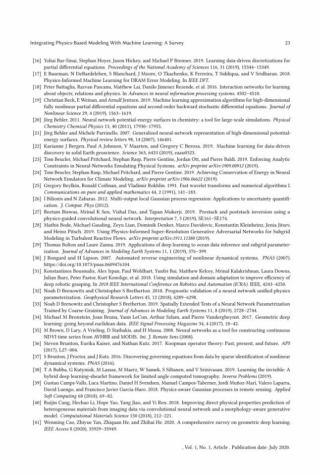
Integrating Physics-Based Modeling With Machine Learning: A Survey 23
[16] Yohai Bar-Sinai, Stephan Hoyer, Jason Hickey, and Michael P Brenner. 2019. Learning data-driven discretizations forpartial differential equations. Proceedings of the National Academy of Sciences 116, 31 (2019), 15344–15349.
[17] E Baseman, N DeBardeleben, S Blanchard, J Moore, O Tkachenko, K Ferreira, T Siddiqua, and V Sridharan. 2018.Physics-Informed Machine Learning for DRAM Error Modeling. In IEEE DFT.
[18] Peter Battaglia, Razvan Pascanu, Matthew Lai, Danilo Jimenez Rezende, et al. 2016. Interaction networks for learningabout objects, relations and physics. In Advances in neural information processing systems. 4502–4510.
[19] Christian Beck, EWeinan, and Arnulf Jentzen. 2019. Machine learning approximation algorithms for high-dimensionalfully nonlinear partial differential equations and second-order backward stochastic differential equations. Journal ofNonlinear Science 29, 4 (2019), 1563–1619.
[20] Jörg Behler. 2011. Neural network potential-energy surfaces in chemistry: a tool for large-scale simulations. PhysicalChemistry Chemical Physics 13, 40 (2011), 17930–17955.
[21] Jörg Behler and Michele Parrinello. 2007. Generalized neural-network representation of high-dimensional potential-energy surfaces. Physical review letters 98, 14 (2007), 146401.
[22] Karianne J Bergen, Paul A Johnson, V Maarten, and Gregory C Beroza. 2019. Machine learning for data-drivendiscovery in solid Earth geoscience. Science 363, 6433 (2019), eaau0323.
[23] Tom Beucler, Michael Pritchard, Stephan Rasp, Pierre Gentine, Jordan Ott, and Pierre Baldi. 2019. Enforcing AnalyticConstraints in Neural-Networks Emulating Physical Systems. arXiv preprint arXiv:1909.00912 (2019).
[24] Tom Beucler, Stephan Rasp, Michael Pritchard, and Pierre Gentine. 2019. Achieving Conservation of Energy in NeuralNetwork Emulators for Climate Modeling. arXiv preprint arXiv:1906.06622 (2019).
[25] Gregory Beylkin, Ronald Coifman, and Vladimir Rokhlin. 1991. Fast wavelet transforms and numerical algorithms I.Communications on pure and applied mathematics 44, 2 (1991), 141–183.
[26] I Bilionis and N Zabaras. 2012. Multi-output local Gaussian process regression: Applications to uncertainty quantifi-cation. J. Comput. Phys (2012).
[27] Reetam Biswas, Mrinal K Sen, Vishal Das, and Tapan Mukerji. 2019. Prestack and poststack inversion using aphysics-guided convolutional neural network. Interpretation 7, 3 (2019), SE161–SE174.
[28] Mathis Bode, Michael Gauding, Zeyu Lian, Dominik Denker, Marco Davidovic, Konstantin Kleinheinz, Jenia Jitsev,and Heinz Pitsch. 2019. Using Physics-Informed Super-Resolution Generative Adversarial Networks for SubgridModeling in Turbulent Reactive Flows. arXiv preprint arXiv:1911.11380 (2019).
[29] Thomas Bolton and Laure Zanna. 2019. Applications of deep learning to ocean data inference and subgrid parameter-ization. Journal of Advances in Modeling Earth Systems 11, 1 (2019), 376–399.
[30] J Bongard and H Lipson. 2007. Automated reverse engineering of nonlinear dynamical systems. PNAS (2007).https://doi.org/10.1073/pnas.0609476104
[31] Konstantinos Bousmalis, Alex Irpan, Paul Wohlhart, Yunfei Bai, Matthew Kelcey, Mrinal Kalakrishnan, Laura Downs,Julian Ibarz, Peter Pastor, Kurt Konolige, et al. 2018. Using simulation and domain adaptation to improve efficiency ofdeep robotic grasping. In 2018 IEEE International Conference on Robotics and Automation (ICRA). IEEE, 4243–4250.
[32] Noah D Brenowitz and Christopher S Bretherton. 2018. Prognostic validation of a neural network unified physicsparameterization. Geophysical Research Letters 45, 12 (2018), 6289–6298.
[33] Noah D Brenowitz and Christopher S Bretherton. 2019. Spatially Extended Tests of a Neural Network ParametrizationTrained by Coarse-Graining. Journal of Advances in Modeling Earth Systems 11, 8 (2019), 2728–2744.
[34] Michael M Bronstein, Joan Bruna, Yann LeCun, Arthur Szlam, and Pierre Vandergheynst. 2017. Geometric deeplearning: going beyond euclidean data. IEEE Signal Processing Magazine 34, 4 (2017), 18–42.
[35] M Brown, D Lary, A Vrieling, D Stathakis, and H Mussa. 2008. Neural networks as a tool for constructing continuousNDVI time series from AVHRR and MODIS. Int. J. Remote Sens (2008).
[36] Steven Brunton, Eurika Kaiser, and Nathan Kutz. 2017. Koopman operator theory: Past, present, and future. APS(2017), L27–004.
[37] S Brunton, J Proctor, and J Kutz. 2016. Discovering governing equations from data by sparse identification of nonlineardynamical systems. PNAS (2016).
[38] T A Bubba, G Kutyniok, M Lassas, M Maerz, W Samek, S Siltanen, and V Srinivasan. 2019. Learning the invisible: Ahybrid deep learning-shearlet framework for limited angle computed tomography. Inverse Problems (2019).
[39] Gustau Camps-Valls, Luca Martino, Daniel H Svendsen, Manuel Campos-Taberner, Jordi Muñoz-Marí, Valero Laparra,David Luengo, and Francisco Javier García-Haro. 2018. Physics-aware Gaussian processes in remote sensing. AppliedSoft Computing 68 (2018), 69–82.
[40] Ruijin Cang, Hechao Li, Hope Yao, Yang Jiao, and Yi Ren. 2018. Improving direct physical properties prediction ofheterogeneous materials from imaging data via convolutional neural network and a morphology-aware generativemodel. Computational Materials Science 150 (2018), 212–221.
[41] Wenming Cao, Zhiyue Yan, Zhiquan He, and Zhihai He. 2020. A comprehensive survey on geometric deep learning.IEEE Access 8 (2020), 35929–35949.
, Vol. 1, No. 1, Article . Publication date: July 2020.

24 Jared Willard, Xiaowei Jia, Shaoming Xu, Michael Steinbach, and Vipin Kumar
[42] Giuseppe Carleo and Matthias Troyer. 2017. Solving the quantum many-body problem with artificial neural networks.Science 355, 6325 (2017), 602–606.
[43] S Chan and A Elsheikh. 2017. Parametrization and generation of geological models with generative adversarialnetworks. arXiv:1708.01810 (2017).
[44] B Chang, M Chen, E Haber, and E Chi. 2019. AntisymmetricRNN: A dynamical system view on recurrent neuralnetworks. arXiv:1902.09689 (2019).
[45] Michael B Chang, Tomer Ullman, Antonio Torralba, and Joshua B Tenenbaum. 2016. A compositional object-basedapproach to learning physical dynamics. arXiv preprint arXiv:1612.00341 (2016).
[46] Gang Chen, Yingtao Zuo, Jian Sun, and Yueming Li. 2012. Support-vector-machine-based reduced-order model forlimit cycle oscillation prediction of nonlinear aeroelastic system. Mathematical problems in engineering 2012 (2012).
[47] H Chen, Y Zhang, M Kalra, F Lin, Y Chen, P Liao, J Zhou, and G Wang. 2017. Low-dose CT with a residual encoder-decoder convolutional neural network. IEEE T-MI (2017).
[48] TQ Chen, Y Rubanova, J Bettencourt, and D K Duvenaud. 2018. Neural ordinary differential equations. In NIPS.[49] W Chen and M Fuge. 2018. BezierGAN: Automatic Generation of Smooth Curves from Interpretable Low-Dimensional
Parameters. arXiv:1808.08871 (2018).[50] X Chen, X Xu, X Liu, S Pan, J He, HY Noh, L Zhang, and P Zhang. 2018. Pga: Physics guided and adaptive approach
for mobile fine-grained air pollution estimation. In Ubicomp.[51] Zhengdao Chen, Jianyu Zhang, Martin Arjovsky, and Léon Bottou. 2019. Symplectic Recurrent Neural Networks.
arXiv preprint arXiv:1909.13334 (2019).[52] In Ho Cho, Qiang Li, Rana Biswas, and Jaeyoun Kim. 2020. A framework for glass-box physics rule learner and its
application to nano-scale phenomena. Communications Physics 3, 1 (2020), 1–9.[53] Youngwoo Cho, Sookyung Kim, Peggy Pk Li, Mike P Surh, T Yong-Jin Han, and Jaegul Choo. 2019. Physics-guided
Reinforcement Learning for 3D Molecular Structures. In Workshop at the 33rd Conference on Neural InformationProcessing Systems (NeurIPS).
[54] Anshul Choudhary, John F Lindner, Elliott G Holliday, Scott T Miller, Sudeshna Sinha, and William L Ditto. 2019.Physics enhanced neural networks predict order and chaos. arXiv preprint arXiv:1912.01958 (2019).
[55] M Christie, V Demyanov, and D Erbas. 2006. Uncertainty quantification for porous media flows. J. Comput. Phys(2006).
[56] Taco S Cohen, Mario Geiger, Jonas Köhler, and Max Welling. 2018. Spherical cnns. arXiv preprint arXiv:1801.10130(2018).
[57] Thomas Daniel, Fabien Casenave, Nissrine Akkari, and David Ryckelynck. 2020. Model order reduction assisted bydeep neural networks (ROM-net). Advanced Modeling and Simulation in Engineering Sciences 7 (2020), 1–27.
[58] A Daw, RQ Thomas, CC Carey, JS Read, AP Appling, and A Karpatne. 2019. Physics-Guided Architecture (PGA) ofNeural Networks for Quantifying Uncertainty in Lake Temperature Modeling. arXiv:1911.02682 (2019).
[59] MS Dawson, J Olvera, AK Fung, and MT Manry. 1992. Inversion of surface parameters using fast learning neuralnetworks. IGARSS International Geoscience and Remote Sensing Symposium (1992).
[60] Emmanuel de Bezenac, Arthur Pajot, and Patrick Gallinari. 2019. Deep learning for physical processes: Incorporatingprior scientific knowledge. Journal of Statistical Mechanics: Theory and Experiment 2019, 12 (2019), 124009.
[61] Nicola De Cao and Thomas Kipf. 2018. MolGAN: An implicit generative model for small molecular graphs. arXivpreprint arXiv:1805.11973 (2018).
[62] L de Oliveira, M Paganini, and B Nachman. 2017. Learning particle physics by example: location-aware generativeadversarial networks for physics synthesis. Comput. Softw. Big Sci (2017).
[63] EL Denton, S Chintala, R Fergus, et al. 2015. Deep generative image models using a laplacian pyramid of adversarialnetworks. In NIPS.
[64] C Deser, A Phillips, V Bourdette, and H Teng. 2012. Uncertainty in climate change projections: the role of internalvariability. Climate dynamics (2012).
[65] MWMG Dissanayake and N Phan-Thien. 1994. Neural-network-based approximations for solving partial differentialequations. communications in Numerical Methods in Engineering 10, 3 (1994), 195–201.
[66] NAK Doan, W Polifke, and L Magri. 2019. Physics-informed echo state networks for chaotic systems forecasting. InICCS. Springer.
[67] B Dong, Z Li, SMM Rahman, and R Vega. 2016. A hybrid model approach for forecasting future residential electricityconsumption. Energy and Buildings (2016).
[68] Jonathan E Downton and Daniel P Hampson. 2019. Use of theory-guided neural networks to perform seismicinversion. In GeoSoftware, CGG.
[69] Vivek Dua. 2011. An artificial neural network approximation based decomposition approach for parameter estimationof system of ordinary differential equations. Computers & chemical engineering 35, 3 (2011), 545–553.
, Vol. 1, No. 1, Article . Publication date: July 2020.
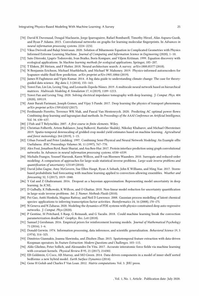
Integrating Physics-Based Modeling With Machine Learning: A Survey 25
[70] David K Duvenaud, Dougal Maclaurin, Jorge Iparraguirre, Rafael Bombarell, Timothy Hirzel, Alán Aspuru-Guzik,and Ryan P Adams. 2015. Convolutional networks on graphs for learning molecular fingerprints. In Advances inneural information processing systems. 2224–2232.
[71] Vikas Dwivedi and Balaji Srinivasan. 2020. Solution of Biharmonic Equation in Complicated Geometries with PhysicsInformed Extreme Learning Machine. Journal of Computing and Information Science in Engineering (2020), 1–10.
[72] Sašo Džeroski, Ljupčo Todorovski, Ivan Bratko, Boris Kompare, and Viljem Križman. 1999. Equation discovery withecological applications. In Machine learning methods for ecological applications. Springer, 185–207.
[73] T Elsken, JH Metzen, and F Hutter. 2018. Neural architecture search: A survey. arXiv:1808.05377 (2018).[74] N Benjamin Erichson, Michael Muehlebach, and Michael W Mahoney. 2019. Physics-informed autoencoders for
lyapunov-stable fluid flow prediction. arXiv preprint arXiv:1905.10866 (2019).[75] James H Faghmous and Vipin Kumar. 2014. A big data guide to understanding climate change: The case for theory-
guided data science. Big data 2, 3 (2014), 155–163.[76] Yuwei Fan, Lin Lin, Lexing Ying, and Leonardo Zepeda-Núnez. 2019. Amultiscale neural network based on hierarchical
matrices. Multiscale Modeling & Simulation 17, 4 (2019), 1189–1213.[77] Yuwei Fan and Lexing Ying. 2020. Solving electrical impedance tomography with deep learning. J. Comput. Phys. 404
(2020), 109119.[78] Amir Barati Farimani, Joseph Gomes, and Vijay S Pande. 2017. Deep learning the physics of transport phenomena.
arXiv preprint arXiv:1709.02432 (2017).[79] Ferdinando Fioretto, Terrence WK Mak, and Pascal Van Hentenryck. 2020. Predicting AC optimal power flows:
Combining deep learning and lagrangian dual methods. In Proceedings of the AAAI Conference on Artificial Intelligence,Vol. 34. 630–637.
[80] J Fish and T Belytschko. 2007. A first course in finite elements. Wiley.[81] Christian Folberth, Artem Baklanov, Juraj Balkovič, Rastislav Skalsky, Nikolay Khabarov, and Michael Obersteiner.
2019. Spatio-temporal downscaling of gridded crop model yield estimates based on machine learning. Agriculturaland forest meteorology 264 (2019), 1–15.
[82] Urban Forssell and Peter Lindskog. 1997. Combining Semi-Physical and Neural Network Modeling: An Example ofItsUsefulness. IFAC Proceedings Volumes 30, 11 (1997), 767–770.
[83] Alex Fout, Jonathon Byrd, Basir Shariat, and Asa Ben-Hur. 2017. Protein interface prediction using graph convolutionalnetworks. In Advances in neural information processing systems. 6530–6539.
[84] Michalis Frangos, Youssef Marzouk, Karen Willcox, and B van Bloemen Waanders. 2010. Surrogate and reduced-ordermodeling: A comparison of approaches for large-scale statistical inverse problems. Large-scale inverse problems andquantification of uncertainty 123149 (2010).
[85] David John Gagne, Amy McGovern, Sue Ellen Haupt, Ryan A Sobash, John K Williams, and Ming Xue. 2017. Storm-based probabilistic hail forecasting with machine learning applied to convection-allowing ensembles. Weather andforecasting 32, 5 (2017), 1819–1840.
[86] Y Gal and Z Ghahramani. 2016. Dropout as a bayesian approximation: Representing model uncertainty in deeplearning. In ICML.
[87] D Galbally, K Fidkowski, K Willcox, and O Ghattas. 2010. Non-linear model reduction for uncertainty quantificationin large-scale inverse problems. Int. J. Numer. Methods Fluids (2010).
[88] Pei Gao, Antti Honkela, Magnus Rattray, and Neil D Lawrence. 2008. Gaussian process modelling of latent chemicalspecies: applications to inferring transcription factor activities. Bioinformatics 24, 16 (2008), i70–i75.
[89] N Geneva and N Zabaras. 2020. Modeling the dynamics of PDE systems with physics-constrained deep auto-regressivenetworks. J. Comput. Phys (2020).
[90] P Gentine, M Pritchard, S Rasp, G Reinaudi, and G Yacalis. 2018. Could machine learning break the convectionparameterization deadlock? Geophys. Res. Lett (2018).
[91] Samuel J Gershman. 2016. Empirical priors for reinforcement learning models. Journal of Mathematical Psychology71 (2016), 1–6.
[92] Donald Gerwin. 1974. Information processing, data inferences, and scientific generalization. Behavioral Science 19, 5(1974), 314–325.
[93] Dimitrios Giannakis, Joanna Slawinska, and Zhizhen Zhao. 2015. Spatiotemporal feature extraction with data-drivenKoopman operators. In Feature Extraction: Modern Questions and Challenges. 103–115.
[94] Aldo Glielmo, Peter Sollich, and Alessandro De Vita. 2017. Accurate interatomic force fields via machine learningwith covariant kernels. Physical Review B 95, 21 (2017), 214302.
[95] EB Goldstein, G Coco, AB Murray, and MO Green. 2014. Data-driven components in a model of inner-shelf sortedbedforms: a new hybrid model. Earth Surface Dynamics (2014).
[96] Gene H Golub and Charles F Van Loan. 2012. Matrix computations. Vol. 3. JHU press.
, Vol. 1, No. 1, Article . Publication date: July 2020.
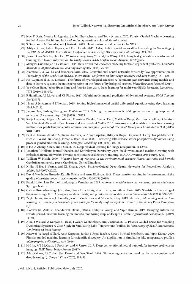
26 Jared Willard, Xiaowei Jia, Shaoming Xu, Michael Steinbach, and Vipin Kumar
[97] Noel P Greis, Monica L Nogueira, Sambit Bhattacharya, and Tony Schmitz. 2020. Physics-Guided Machine Learningfor Self-Aware Machining. In AAAI Spring Symposium – AI and Manufacturing.
[98] S Greydanus, M Dzamba, and J Yosinski. 2019. Hamiltonian neural networks. In NIPS.[99] Aditya Grover, Ashish Kapoor, and Eric Horvitz. 2015. A deep hybrid model for weather forecasting. In Proceedings of
the 21th ACM SIGKDD International Conference on Knowledge Discovery and Data Mining. 379–386.[100] Jiaxian Guo, Sidi Lu, Han Cai, Weinan Zhang, Yong Yu, and Jun Wang. 2018. Long text generation via adversarial
training with leaked information. In Thirty-Second AAAI Conference on Artificial Intelligence.[101] Mengwu Guo and Jan S Hesthaven. 2019. Data-driven reduced order modeling for time-dependent problems. Computer
Methods in Applied Mechanics and Engineering 345 (2019), 75–99.[102] Xiaoxiao Guo, Wei Li, and Francesco Iorio. 2016. Convolutional neural networks for steady flow approximation. In
Proceedings of the 22nd ACM SIGKDD international conference on knowledge discovery and data mining. 481–490.[103] HV Gupta et al. 2014. Debates—The future of hydrological sciences: A (common) path forward? Using models and
data to learn: A systems theoretic perspective on the future of hydrological science. Water Resources Research (2014).[104] Yoo-Geun Ham, Jeong-Hwan Kim, and Jing-Jia Luo. 2019. Deep learning for multi-year ENSO forecasts. Nature 573,
7775 (2019), 568–572.[105] F Hamilton, AL Lloyd, and KB Flores. 2017. Hybrid modeling and prediction of dynamical systems. PLOS Comput.
Biol (2017).[106] J Han, A Jentzen, and E Weinan. 2018. Solving high-dimensional partial differential equations using deep learning.
PNAS (2018).[107] Jiequn Han, Linfeng Zhang, and E Weinan. 2019. Solving many-electron Schrödinger equation using deep neural
networks. J. Comput. Phys. 399 (2019), 108929.[108] Katja Hansen, Grégoire Montavon, Franziska Biegler, Siamac Fazli, Matthias Rupp, Matthias Scheffler, O Anatole
Von Lilienfeld, Alexandre Tkatchenko, and Klaus-Robert Muller. 2013. Assessment and validation of machine learningmethods for predicting molecular atomization energies. Journal of Chemical Theory and Computation 9, 8 (2013),3404–3419.
[109] Paul C Hanson, Aviah B Stillman, Xiaowei Jia, Anuj Karpatne, Hilary A Dugan, Cayelan C Carey, Joseph Stachelek,Nicole K Ward, Yu Zhang, Jordan S Read, et al. 2020. Predicting lake surface water phosphorus dynamics usingprocess-guided machine learning. Ecological Modelling 430 (2020), 109136.
[110] K He, X Zhang, S Ren, and J Sun. 2016. Deep residual learning for image recognition. In CVPR.[111] Jonathan R Holland, James D Baeder, and Karthikeyan Duraisamy. 2019. Field inversion and machine learning with
embedded neural networks: Physics-consistent neural network training. In AIAA Aviation 2019 Forum. 3200.[112] William W Hsieh. 2009. Machine learning methods in the environmental sciences: Neural networks and kernels.
Cambridge university press, Cambridge, United Kingdom.[113] X Hu, H Hu, S Verma, and ZL Zhang. 2020. Physics-Guided Deep Neural Networks for PowerFlow Analysis.
arXiv:2002.00097 (2020).[114] David Menéndez Hurtado, Karolis Uziela, and Arne Elofsson. 2018. Deep transfer learning in the assessment of the
quality of protein models. arXiv preprint arXiv:1804.06281 (2018).[115] Frank Hutter, Lars Kotthoff, and Joaquin Vanschoren. 2019. Automated machine learning: methods, systems, challenges.
Springer Nature.[116] Gabriel Ibarra-Berastegi, Jon Saénz, Ganix Esnaola, Agustin Ezcurra, and Alain Ulazia. 2015. Short-term forecasting of
the wave energy flux: Analogues, random forests, and physics-based models. Ocean Engineering 104 (2015), 530–539.[117] Željko Ivezić, Andrew J Connolly, Jacob T VanderPlas, and Alexander Gray. 2019. Statistics, data mining, and machine
learning in astronomy: a practical Python guide for the analysis of survey data. Princeton University Press, Princeton,NJ.
[118] Xiaowei Jia, Ankush Khandelwal, David J Mulla, Philip G Pardey, and Vipin Kumar. 2019. Bringing automated,remote-sensed, machine learning methods to monitoring crop landscapes at scale. Agricultural Economics 50 (2019),41–50.
[119] X Jia, J Willard, A Karpatne, J Read, J Zwart, M Steinbach, and V Kumar. 2019. Physics Guided RNNs for ModelingDynamical Systems: A Case Study in Simulating Lake Temperature Profiles. In Proceedings of SIAM InternationalConference on Data Mining.
[120] Xiaowei Jia, Jared Willard, Anuj Karpatne, Jordan S Read, Jacob A Zwart, Michael Steinbach, and Vipin Kumar. 2020.Physics-guided machine learning for scientific discovery: An application in simulating lake temperature profiles.arXiv preprint arXiv:2001.11086 (2020).
[121] KH Jin, MT McCann, E Froustey, and M Unser. 2017. Deep convolutional neural network for inverse problems inimaging. IEEE Trans. Image Process (2017).
[122] Adar Kahana, Eli Turkel, Shai Dekel, and Dan Givoli. 2020. Obstacle segmentation based on the wave equation anddeep learning. J. Comput. Phys. (2020), 109458.
, Vol. 1, No. 1, Article . Publication date: July 2020.

Integrating Physics-Based Modeling With Machine Learning: A Survey 27
[123] Eurika Kaiser, J Nathan Kutz, and Steven L Brunton. 2018. Sparse identification of nonlinear dynamics for modelpredictive control in the low-data limit. Proceedings of the Royal Society A 474, 2219 (2018), 20180335.
[124] Eugenia Kalnay. 2003. Atmospheric modeling, data assimilation and predictability. Cambridge university press.[125] J Kani and A Elsheikh. 2017. DR-RNN: A deep residual recurrent neural network for model reduction. arXiv:1709.00939
(2017).[126] Anuj Karpatne, Gowtham Atluri, James H Faghmous, Michael Steinbach, Arindam Banerjee, Auroop Ganguly, Shashi
Shekhar, Nagiza Samatova, and Vipin Kumar. 2017. Theory-guided data science: A new paradigm for scientificdiscovery from data. IEEE Transactions on knowledge and data engineering 29, 10 (2017), 2318–2331.
[127] Anuj Karpatne, Imme Ebert-Uphoff, Sai Ravela, Hassan Ali Babaie, and Vipin Kumar. 2018. Machine learning forthe geosciences: Challenges and opportunities. IEEE Transactions on Knowledge and Data Engineering 31, 8 (2018),1544–1554.
[128] A Karpatne, W Watkins, J Read, and V Kumar. 2017. Physics-guided Neural Networks (PGNN): An Application inLake Temperature Modeling. arXiv:1710.11431 (2017).
[129] S Karumuri, R Tripathy, I Bilionis, and J Panchal. 2020. Simulator-free solution of high-dimensional stochastic ellipticpartial differential equations using deep neural networks. J. Comput. Phys (2020).
[130] Steven K Kauwe, Jake Graser, Antonio Vazquez, and Taylor D Sparks. 2018. Machine learning prediction of heatcapacity for solid inorganics. Integrating Materials and Manufacturing Innovation 7, 2 (2018), 43–51.
[131] Yuehaw Khoo, Jianfeng Lu, and Lexing Ying. 2019. Solving for high-dimensional committor functions using artificialneural networks. Research in the Mathematical Sciences 6, 1 (2019), 1.
[132] Yuehaw Khoo and Lexing Ying. 2019. SwitchNet: a neural network model for forward and inverse scattering problems.SIAM Journal on Scientific Computing 41, 5 (2019), A3182–A3201.
[133] Byungsoo Kim, Vinicius C Azevedo, Nils Thuerey, Theodore Kim, Markus Gross, and Barbara Solenthaler. 2019. Deepfluids: A generative network for parameterized fluid simulations. In Computer Graphics Forum, Vol. 38. Wiley OnlineLibrary, 59–70.
[134] Hiroshi Koizumi, Seiji Tsutsumi, and Eiji Shima. 2018. Feedback control of Karman vortex shedding from a cylinderusing deep reinforcement learning. In 2018 Flow Control Conference. 3691.
[135] Vladimir M Krasnopolsky and Michael S Fox-Rabinovitz. 2006. Complex hybrid models combining deterministic andmachine learning components for numerical climate modeling and weather prediction. Neural Networks 19, 2 (2006),122–134.
[136] Sofia Ira Ktena, Sarah Parisot, Enzo Ferrante, Martin Rajchl, Matthew Lee, Ben Glocker, and Daniel Rueckert.2017. Distance metric learning using graph convolutional networks: Application to functional brain networks. InInternational Conference on Medical Image Computing and Computer-Assisted Intervention. Springer, 469–477.
[137] Siddhant Kumar, Stephanie Tan, Li Zheng, and Dennis M Kochmann. 2020. Inverse-designed spinodoid metamaterials.npj Computational Materials 6, 1 (2020), 1–10.
[138] J Nathan Kutz. 2017. Deep learning in fluid dynamics. Journal of Fluid Mechanics 814 (2017), 1–4.[139] L’ubor Ladicky, SoHyeon Jeong, Barbara Solenthaler, Marc Pollefeys, and Markus Gross. 2015. Data-driven fluid
simulations using regression forests. ACM Transactions on Graphics (TOG) 34, 6 (2015), 1–9.[140] IE Lagaris, A Likas, and DI Fotiadis. 1998. Artificial neural networks for solving ordinary and partial differential
equations. IEEE Trans. Neural Netw. Learn (1998).[141] John H Lagergren, John T Nardini, G Michael Lavigne, Erica M Rutter, and Kevin B Flores. 2020. Learning partial
differential equations for biological transport models from noisy spatio-temporal data. Proceedings of the Royal SocietyA 476, 2234 (2020), 20190800.
[142] B Lakshminarayanan, A Pritzel, and C Blundell. 2017. Simple and scalable predictive uncertainty estimation usingdeep ensembles. In NIPS.
[143] Pat Langley. 1981. Data-driven discovery of physical laws. Cognitive Science 5, 1 (1981), 31–54.[144] Pat Langley, Gary L Bradshaw, and Herbert A Simon. 1983. Rediscovering chemistry with the BACON system. In
Machine learning. Springer, 307–329.[145] Toni Lassila, Andrea Manzoni, Alfio Quarteroni, and Gianluigi Rozza. 2014. Model order reduction in fluid dynamics:
challenges and perspectives. In Reduced Order Methods for modeling and computational reduction. Springer, 235–273.[146] Neil D Lawrence, Guido Sanguinetti, and Magnus Rattray. 2007. Modelling transcriptional regulation using Gaussian
processes. In Advances in Neural Information Processing Systems. 785–792.[147] Hyuk Lee and In Seok Kang. 1990. Neural algorithm for solving differential equations. J. Comput. Phys. 91, 1 (1990),
110–131.[148] Kookjin Lee and Kevin T Carlberg. 2020. Model reduction of dynamical systems on nonlinear manifolds using deep
convolutional autoencoders. J. Comput. Phys. 404 (2020), 108973.[149] Douglas B Lenat. 1983. The role of heuristics in learning by discovery: Three case studies. In Machine learning.
Springer, 243–306.
, Vol. 1, No. 1, Article . Publication date: July 2020.
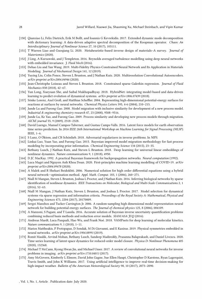
28 Jared Willard, Xiaowei Jia, Shaoming Xu, Michael Steinbach, and Vipin Kumar
[150] Qianxiao Li, Felix Dietrich, Erik M Bollt, and Ioannis G Kevrekidis. 2017. Extended dynamic mode decompositionwith dictionary learning: A data-driven adaptive spectral decomposition of the Koopman operator. Chaos: AnInterdisciplinary Journal of Nonlinear Science 27, 10 (2017), 103111.
[151] T Warren Liao and Guoqiang Li. 2020. Metaheuristic-based inverse design of materials–A survey. Journal ofMateriomics (2020).
[152] J Ling, A Kurzawski, and J Templeton. 2016. Reynolds averaged turbulence modelling using deep neural networkswith embedded invariance. J. Fluid Mech (2016).
[153] Dehao Liu and Yan Wang. 2019. Multi-Fidelity Physics-Constrained Neural Network and Its Application in MaterialsModeling. Journal of Mechanical Design 141, 12 (2019).
[154] Yuying Liu, Colin Ponce, Steven L Brunton, and J Nathan Kutz. 2020. Multiresolution Convolutional Autoencoders.arXiv preprint arXiv:2004.04946 (2020).
[155] Jean-Christophe Loiseau and Steven L Brunton. 2018. Constrained sparse Galerkin regression. Journal of FluidMechanics 838 (2018), 42–67.
[156] Yun Long, Xueyuan She, and Saibal Mukhopadhyay. 2018. HybridNet: integrating model-based and data-drivenlearning to predict evolution of dynamical systems. arXiv preprint arXiv:1806.07439 (2018).
[157] Sönke Lorenz, Axel Groß, and Matthias Scheffler. 2004. Representing high-dimensional potential-energy surfaces forreactions at surfaces by neural networks. Chemical Physics Letters 395, 4-6 (2004), 210–215.
[158] Junde Lu and Furong Gao. 2008. Model migration with inclusive similarity for development of a new process model.Industrial & engineering chemistry research 47, 23 (2008), 9508–9516.
[159] Junde Lu, Ke Yao, and Furong Gao. 2009. Process similarity and developing new process models through migration.AIChE journal 55, 9 (2009), 2318–2328.
[160] David Luengo, Manuel Campos-Taberner, and Gustau Camps-Valls. 2016. Latent force models for earth observationtime series prediction. In 2016 IEEE 26th International Workshop on Machine Learning for Signal Processing (MLSP).IEEE, 1–6.
[161] S Lunz, O Öktem, and CB Schönlieb. 2018. Adversarial regularizers in inverse problems. In NIPS.[162] Linkai Luo, Yuan Yao, and Furong Gao. 2015. Bayesian improved model migration methodology for fast process
modeling by incorporating prior information. Chemical Engineering Science 134 (2015), 23–35.[163] Bethany Lusch, J Nathan Kutz, and Steven L Brunton. 2018. Deep learning for universal linear embeddings of
nonlinear dynamics. Nature communications 9, 1 (2018), 4950.[164] D JC MacKay. 1992. A practical Bayesian framework for backpropagation networks. Neural computation (1992).[165] Luca Magri and Nguyen Anh Khoa Doan. 2020. First-principles machine learning modelling of COVID-19. arXiv
preprint arXiv:2004.09478 (2020).[166] A Malek and R Shekari Beidokhti. 2006. Numerical solution for high order differential equations using a hybrid
neural network—optimization method. Appl. Math. Comput. 183, 1 (2006), 260–271.[167] Niall M Mangan, Steven L Brunton, Joshua L Proctor, and J Nathan Kutz. 2016. Inferring biological networks by sparse
identification of nonlinear dynamics. IEEE Transactions on Molecular, Biological and Multi-Scale Communications 2, 1(2016), 52–63.
[168] Niall M Mangan, J Nathan Kutz, Steven L Brunton, and Joshua L Proctor. 2017. Model selection for dynamicalsystems via sparse regression and information criteria. Proceedings of the Royal Society A: Mathematical, Physical andEngineering Sciences 473, 2204 (2017), 20170009.
[169] Sergei Manzhos and Tucker Carrington Jr. 2006. A random-sampling high dimensional model representation neuralnetwork for building potential energy surfaces. The Journal of chemical physics 125, 8 (2006), 084109.
[170] A Manzoni, S Pagani, and T Lassila. 2016. Accurate solution of Bayesian inverse uncertainty quantification problemscombining reduced basis methods and reduction error models. SIAM/ASA JUQ (2016).
[171] Andreas Mardt, Luca Pasquali, Hao Wu, and Frank Noé. 2018. VAMPnets for deep learning of molecular kinetics.Nature communications 9, 1 (2018), 1–11.
[172] Marios Mattheakis, P Protopapas, D Sondak, M Di Giovanni, and E Kaxiras. 2019. Physical symmetries embedded inneural networks. arXiv preprint arXiv:1904.08991 (2019).
[173] Romit Maulik, Arvind Mohan, Bethany Lusch, Sandeep Madireddy, Prasanna Balaprakash, and Daniel Livescu. 2020.Time-series learning of latent-space dynamics for reduced-order model closure. Physica D: Nonlinear Phenomena 405(2020), 132368.
[174] Michael T McCann, Kyong Hwan Jin, and Michael Unser. 2017. A review of convolutional neural networks for inverseproblems in imaging. arXiv preprint arXiv:1710.04011 (2017).
[175] Amy McGovern, Kimberly L Elmore, David John Gagne, Sue Ellen Haupt, Christopher D Karstens, Ryan Lagerquist,Travis Smith, and John K Williams. 2017. Using artificial intelligence to improve real-time decision-making forhigh-impact weather. Bulletin of the American Meteorological Society 98, 10 (2017), 2073–2090.
, Vol. 1, No. 1, Article . Publication date: July 2020.
Integrating Physics-Based Modeling With Machine Learning: A Survey 29
[176] Xuhui Meng and George Em Karniadakis. 2020. A composite neural network that learns from multi-fidelity data:Application to function approximation and inverse PDE problems. J. Comput. Phys. 401 (2020), 109020.
[177] X Meng, Z Li, D Zhang, and GE Karniadakis. 2019. Ppinn: Parareal physics-informed neural network for time-dependent pdes. arXiv:1909.10145 (2019).
[178] Igor Mezić. 2005. Spectral properties of dynamical systems, model reduction and decompositions. Nonlinear Dynamics41, 1-3 (2005), 309–325.
[179] Arvind T Mohan and Datta V Gaitonde. 2018. A deep learning based approach to reduced order modeling for turbulentflow control using LSTM neural networks. arXiv preprint arXiv:1804.09269 (2018).
[180] Jeremy Morton, Freddie D Witherden, and Mykel J Kochenderfer. 2019. Deep variational koopman models: Inferringkoopman observations for uncertainty-aware dynamics modeling and control. arXiv preprint arXiv:1902.09742 (2019).
[181] Mayur Mudigonda, Sookyung Kim, Ankur Mahesh, Samira Kahou, Karthik Kashinath, Dean Williams, VincenMichalski, Travis O’Brien, and Mr Prabhat. 2017. Segmenting and tracking extreme climate events using neuralnetworks. In Deep Learning for Physical Sciences (DLPS) Workshop, held with NIPS Conference.
[182] Nikhil Muralidhar, Jie Bu, Ze Cao, Long He, Naren Ramakrishnan, Danesh Tafti, and Anuj Karpatne. 2020. PhyNet:Physics Guided Neural Networks for Particle Drag Force Prediction in Assembly. In Proceedings of the 2020 SIAMInternational Conference on Data Mining. SIAM, 559–567.
[183] N Muralidhar, MR Islam, M Marwah, A Karpatne, and N Ramakrishnan. 2018. Incorporating prior domain knowledgeinto deep neural networks. In IEEE Big Data. IEEE.
[184] Frank Noé, Alexandre Tkatchenko, Klaus-Robert Müller, and Cecilia Clementi. 2020. Machine learning for molecularsimulation. Annual review of physical chemistry 71 (2020), 361–390.
[185] Peer Nowack, Peter Braesicke, Joanna Haigh, Nathan Luke Abraham, John Pyle, and Apostolos Voulgarakis. 2018.Using machine learning to build temperature-based ozone parameterizations for climate sensitivity simulations.Environmental Research Letters 13, 10 (2018), 104016.
[186] Paul A O’Gorman and John G Dwyer. 2018. Using machine learning to parameterize moist convection: Potential formodeling of climate, climate change, and extreme events. Journal of Advances in Modeling Earth Systems 10, 10 (2018),2548–2563.
[187] A Oord, S Dieleman, H Zen, K Simonyan, O Vinyals, A Graves, N Kalchbrenner, A Senior, and K Kavukcuoglu. 2016.Wavenet: A generative model for raw audio. arXiv:1609.03499 (2016).
[188] Samuel E Otto and Clarence W Rowley. 2019. Linearly recurrent autoencoder networks for learning dynamics. SIAMJournal on Applied Dynamical Systems 18, 1 (2019), 558–593.
[189] Anikesh Pal. [n.d.]. Deep learning emulation of subgrid scale processes in turbulent shear flows. Geophysical ResearchLetters ([n. d.]), e2020GL087005.
[190] Shaowu Pan and Karthik Duraisamy. 2020. Physics-informed probabilistic learning of linear embeddings of nonlineardynamics with guaranteed stability. SIAM Journal on Applied Dynamical Systems 19, 1 (2020), 480–509.
[191] R Paolucci, F Gatti, M Infantino, C Smerzini, AG Özcebe, and M Stupazzini. 2018. Broadband Ground Motions from3D Physics-Based Numerical Simulations Using Artificial Neural NetworksBroadband Ground Motions from 3D PBSsUsing ANNs. BSSA (2018).
[192] EJ Parish and K Duraisamy. 2016. A paradigm for data-driven predictive modeling using field inversion and machinelearning. J. Comput. Phys (2016).
[193] Junyoung Park and Jinkyoo Park. 2019. Physics-induced graph neural network: An application to wind-farm powerestimation. Energy 187 (2019), 115883.
[194] Wei Peng, Weien Zhou, Jun Zhang, and Wen Yao. 2020. Accelerating Physics-Informed Neural Network Trainingwith Prior Dictionaries. arXiv preprint arXiv:2004.08151 (2020).
[195] CL Pettit. 2004. Uncertainty quantification in aeroelasticity: recent results and research challenges. Journal of Aircraft(2004).
[196] David Pfau, James S Spencer, Alexander G de G Matthews, and WMC Foulkes. 2019. Ab-Initio Solution of theMany-Electron Schr\" odinger Equation with Deep Neural Networks. arXiv preprint arXiv:1909.02487 (2019).
[197] L Pilozzi, FA Farrelly, G Marcucci, and C Conti. 2018. Machine learning inverse problem for topological photonics.Communications Physics (2018).
[198] Frederico V Prudente and JJ Soares Neto. 1998. The fitting of potential energy surfaces using neural networks.Application to the study of the photodissociation processes. Chemical physics letters 287, 5-6 (1998), 585–589.
[199] A Pukrittayakamee, M Malshe, M Hagan, LM Raff, R Narulkar, S Bukkapatnum, and R Komanduri. 2009. Simultaneousfitting of a potential-energy surface and its corresponding force fields using feedforward neural networks. J. Chem.Phys (2009).
[200] Markus Quade, Markus Abel, J Nathan Kutz, and Steven L Brunton. 2018. Sparse identification of nonlinear dynamicsfor rapid model recovery. Chaos: An Interdisciplinary Journal of Nonlinear Science 28, 6 (2018), 063116.
, Vol. 1, No. 1, Article . Publication date: July 2020.
30 Jared Willard, Xiaowei Jia, Shaoming Xu, Michael Steinbach, and Vipin Kumar
[201] Alfio Quarteroni, Gianluigi Rozza, et al. 2014. Reduced order methods for modeling and computational reduction. Vol. 9.Springer.
[202] Paul Raccuglia, Katherine C Elbert, Philip DF Adler, Casey Falk, Malia B Wenny, Aurelio Mollo, Matthias Zeller,Sorelle A Friedler, Joshua Schrier, and Alexander J Norquist. 2016. Machine-learning-assisted materials discoveryusing failed experiments. Nature 533, 7601 (2016), 73–76.
[203] LM Raff, M Malshe, M Hagan, DI Doughan, MG Rockley, and R Komanduri. 2005. Ab initio potential-energy surfacesfor complex, multichannel systems using modified novelty sampling and feedforward neural networks. The Journalof chemical physics 122, 8 (2005), 084104.
[204] Rahul Rai and Chandan K Sahu. 2020. Driven by Data or Derived Through Physics? A Review of Hybrid PhysicsGuided Machine Learning Techniques With Cyber-Physical System (CPS) Focus. IEEE Access 8 (2020), 71050–71073.
[205] Maziar Raissi. 2018. Deep hidden physics models: Deep learning of nonlinear partial differential equations. TheJournal of Machine Learning Research 19, 1 (2018), 932–955.
[206] Maziar Raissi and George Em Karniadakis. 2018. Hidden physics models: Machine learning of nonlinear partialdifferential equations. J. Comput. Phys. 357 (2018), 125–141.
[207] M Raissi, P Perdikaris, and GE Karniadakis. 2017. Physics informed deep learning (part II): Data-driven discovery ofnonlinear partial differential equations. arXiv:1711.10561 (2017).
[208] M Raissi, P Perdikaris, and GE Karniadakis. 2019. Physics-informed neural networks: A deep learning framework forsolving forward and inverse problems involving nonlinear partial differential equations. J. Comput. Phys (2019).
[209] Maziar Raissi, Paris Perdikaris, and George Em Karniadakis. 2017. Physics informed deep learning (part i): Data-drivensolutions of nonlinear partial differential equations. arXiv preprint arXiv:1711.10561 (2017).
[210] M Raissi, Z Wang, M Triantafyllou, and G Karniadakis. 2019. Deep learning of vortex-induced vibrations. J. FluidMech (2019).
[211] MM Rajabi and H Ketabchi. 2017. Uncertainty-based simulation-optimization using Gaussian process emulation:application to coastal groundwater management. J. Hydrol (2017).
[212] Stephan Rasp, Michael S Pritchard, and Pierre Gentine. 2018. Deep learning to represent subgrid processes in climatemodels. Proceedings of the National Academy of Sciences 115, 39 (2018), 9684–9689.
[213] JS Read, X Jia, J Willard, AP Appling, JA Zwart, SK Oliver, A Karpatne, GJA Hansen, PC Hanson, W Watkins, et al.2019. Process-guided deep learning predictions of lake water temperature. Water Resources Research (2019).
[214] Markus Reichstein, Gustau Camps-Valls, Bjorn Stevens, Martin Jung, Joachim Denzler, Nuno Carvalhais, et al. 2019.Deep learning and process understanding for data-driven Earth system science. Nature 566, 7743 (2019), 195–204.
[215] K Rudd and S Ferrari. 2015. A constrained integration (CINT) approach to solving partial differential equations usingartificial neural networks. Neurocomputing (2015).
[216] SH Rudy, SL Brunton, JL Proctor, and JN Kutz. 2017. Data-driven discovery of partial differential equations. ScienceAdvances (2017).
[217] Samuel H Rudy, J Nathan Kutz, and Steven L Brunton. 2019. Deep learning of dynamics and signal-noise decompositionwith time-stepping constraints. J. Comput. Phys. 396 (2019), 483–506.
[218] L Ruthotto and E Haber. 2018. Deep neural networks motivated by partial differential equations. Journal ofMathematical Imaging and Vision (2018).
[219] Jonathan J Rutz, Christine A Shields, Juan M Lora, Ashley E Payne, Bin Guan, Paul Ullrich, Travis O’Brien, L RubyLeung, F Martin Ralph, Michael Wehner, et al. 2019. The atmospheric river tracking method intercomparison project(ARTMIP): quantifying uncertainties in atmospheric river climatology. Journal of Geophysical Research: Atmospheres(2019).
[220] Kevin Ryan, Jeff Lengyel, and Michael Shatruk. 2018. Crystal structure prediction via deep learning. Journal of theAmerican Chemical Society 140, 32 (2018), 10158–10168.
[221] M Sadoughi and C Hu. 2019. Physics-based convolutional neural network for fault diagnosis of rolling elementbearings. IEEE Sensors Journal (2019).
[222] Peter Sadowski, David Fooshee, Niranjan Subrahmanya, and Pierre Baldi. 2016. Synergies Between QuantumMechanics and Machine Learning in Reaction Prediction. Journal of Chemical Information and Modeling 56, 11 (2016),2125–2128. https://doi.org/10.1021/acs.jcim.6b00351 arXiv:https://doi.org/10.1021/acs.jcim.6b00351 PMID: 27749058.
[223] O San and RMaulik. 2018. Machine learning closures for model order reduction of thermal fluids. Applied MathematicalModelling (2018).
[224] Omer San and Romit Maulik. 2018. Neural network closures for nonlinear model order reduction. Advances inComputational Mathematics 44, 6 (2018), 1717–1750.
[225] Omer San, Romit Maulik, and Mansoor Ahmed. 2019. An artificial neural network framework for reduced ordermodeling of transient flows. Communications in Nonlinear Science and Numerical Simulation 77 (2019), 271–287.
[226] Gabriel R Schleder, Antonio CM Padilha, Carlos Mera Acosta, Marcio Costa, and Adalberto Fazzio. 2019. From DFT tomachine learning: recent approaches to materials science–a review. Journal of Physics: Materials 2, 3 (2019), 032001.
, Vol. 1, No. 1, Article . Publication date: July 2020.
Integrating Physics-Based Modeling With Machine Learning: A Survey 31
[227] M Schmidt and H Lipson. 2009. Distilling free-form natural laws from experimental data. Science (2009).[228] Kristof Schütt, Pieter-Jan Kindermans, Huziel Enoc Sauceda Felix, Stefan Chmiela, Alexandre Tkatchenko, and Klaus-
Robert Müller. 2017. Schnet: A continuous-filter convolutional neural network for modeling quantum interactions. InAdvances in neural information processing systems. 991–1001.
[229] O Senouf, S Vedula, T Weiss, A Bronstein, O Michailovich, and M Zibulevsky. 2019. Self-supervised learning ofinverse problem solvers in medical imaging. In Domain Adaptation and Representation Transfer and Medical ImageLearning with Less Labels and Imperfect Data. Springer.
[230] Shital Shah, Debadeepta Dey, Chris Lovett, and Ashish Kapoor. 2018. Airsim: High-fidelity visual and physicalsimulation for autonomous vehicles. In Field and service robotics. Springer, 621–635.
[231] V Shah, A Joshi, S Ghosal, B Pokuri, S Sarkar, B Ganapathysubramanian, and C Hegde. 2019. Encoding invariances indeep generative models. arXiv:1906.01626 (2019).
[232] Ehsan Sharifi, B Saghafian, and R Steinacker. 2019. Downscaling satellite precipitation estimates with multiplelinear regression, artificial neural networks, and spline interpolation techniques. Journal of Geophysical Research:Atmospheres 124, 2 (2019), 789–805.
[233] Ati S Sharma, Igor Mezić, and Beverley J McKeon. 2016. Correspondence between Koopman mode decomposition,resolvent mode decomposition, and invariant solutions of the Navier-Stokes equations. Physical Review Fluids 1, 3(2016), 032402.
[234] R Sharma, AB Farimani, J Gomes, P Eastman, and V Pande. 2018. Weakly-supervised deep learning of heat transportvia physics informed loss. arXiv:1807.11374 (2018).
[235] Justin Sirignano and Konstantinos Spiliopoulos. 2018. DGM: A deep learning algorithm for solving partial differentialequations. J. Comput. Phys. 375 (2018), 1339–1364.
[236] D Solle, B Hitzmann, C Herwig, M Pereira R, S Ulonska, L Wuerth, A Prata, and T Steckenreiter. 2017. Between thepoles of data-driven and mechanistic modeling for process operation. Chemie Ingenieur Technik (2017).
[237] Prashant K Srivastava, Dawei Han, Miguel Rico Ramirez, and Tanvir Islam. 2013. Machine learning techniques fordownscaling SMOS satellite soil moisture using MODIS land surface temperature for hydrological application. Waterresources management 27, 8 (2013), 3127–3144.
[238] P Sturmfels, S Rutherford, M Angstadt, M Peterson, C Sripada, and J Wiens. 2018. A domain guided CNN architecturefor predicting age from structural brain images. arXiv:1808.04362 (2018).
[239] Mohammad M Sultan, Hannah K Wayment-Steele, and Vijay S Pande. 2018. Transferable neural networks forenhanced sampling of protein dynamics. Journal of chemical theory and computation 14, 4 (2018), 1887–1894.
[240] Jian Sun, Zhan Niu, Kristopher A Innanen, Junxiao Li, and Daniel O Trad. 2020. A theory-guided deep-learningformulation and optimization of seismic waveform inversion. Geophysics 85, 2 (2020), R87–R99.
[241] Daniel Heestermans Svendsen, Luca Martino, Manuel Campos-Taberner, Francisco Javier García-Haro, and GustauCamps-Valls. 2017. Joint Gaussian processes for biophysical parameter retrieval. IEEE Transactions on Geoscience andRemote Sensing 56, 3 (2017), 1718–1727.
[242] Laura Swiler, Mamikon Gulian, Ari Frankel, Cosmin Safta, and John Jakeman. 2020. A Survey of Constrained GaussianProcess Regression: Approaches and Implementation Challenges. arXiv preprint arXiv:2006.09319 (2020).
[243] Nima Tajbakhsh, Jae Y Shin, Suryakanth R Gurudu, R Todd Hurst, Christopher B Kendall, Michael B Gotway, andJianming Liang. 2016. Convolutional neural networks for medical image analysis: Full training or fine tuning? IEEEtransactions on medical imaging 35, 5 (2016), 1299–1312.
[244] Naoya Takeishi, Yoshinobu Kawahara, and Takehisa Yairi. 2017. Learning Koopman invariant subspaces for dynamicmode decomposition. In Advances in Neural Information Processing Systems. 1130–1140.
[245] Christian Tesche, Carlo N De Cecco, Stefan Baumann, Matthias Renker, Tindal W McLaurin, Taylor M Duguay,Richard R Bayer 2nd, Daniel H Steinberg, Katharine L Grant, Christian Canstein, et al. 2018. Coronary CT angiography–derived fractional flow reserve: machine learning algorithm versus computational fluid dynamics modeling. Radiology288, 1 (2018), 64–72.
[246] Nathaniel Thomas, Tess Smidt, Steven Kearnes, Lusann Yang, Li Li, Kai Kohlhoff, and Patrick Riley. 2018. Tensor fieldnetworks: Rotation-and translation-equivariant neural networks for 3d point clouds. arXiv preprint arXiv:1802.08219(2018).
[247] Michael L Thompson and Mark A Kramer. 1994. Modeling chemical processes using prior knowledge and neuralnetworks. AIChE Journal 40, 8 (1994), 1328–1340.
[248] Josh Tobin, Rachel Fong, Alex Ray, Jonas Schneider,Wojciech Zaremba, and Pieter Abbeel. 2017. Domain randomizationfor transferring deep neural networks from simulation to the real world. In 2017 IEEE/RSJ international conference onintelligent robots and systems (IROS). IEEE, 23–30.
[249] Peter Toth, Danilo Jimenez Rezende, Andrew Jaegle, Sébastien Racanière, Aleksandar Botev, and Irina Higgins. 2019.Hamiltonian generative networks. arXiv preprint arXiv:1909.13789 (2019).
, Vol. 1, No. 1, Article . Publication date: July 2020.
32 Jared Willard, Xiaowei Jia, Shaoming Xu, Michael Steinbach, and Vipin Kumar
[250] RK Tripathy and I Bilionis. 2018. Deep UQ: Learning deep neural network surrogate models for high dimensionaluncertainty quantification. J. Comput. Phys (2018).
[251] Silviu-Marian Udrescu and Max Tegmark. 2020. AI Feynman: A physics-inspired method for symbolic regression.Science Advances 6, 16 (2020), eaay2631.
[252] D Ulyanov, A Vedaldi, and V Lempitsky. 2018. Deep image prior. In CVPR.[253] J Vamaraju and MK Sen. 2019. Unsupervised physics-based neural networks for seismic migration. Interpretation
(2019).[254] Thomas Vandal, Evan Kodra, Sangram Ganguly, Andrew Michaelis, Ramakrishna Nemani, and Auroop R Ganguly.
2017. Deepsd: Generating high resolution climate change projections through single image super-resolution. InProceedings of the 23rd acm sigkdd international conference on knowledge discovery and data mining. 1663–1672.
[255] PR Vlachas, W Byeon, ZY Wan, TP Sapsis, and P Koumoutsakos. 2018. Data-driven forecasting of high-dimensionalchaotic systems with long short-term memory networks. Proc. R. Soc. A (2018).
[256] Laura von Rueden, Sebastian Mayer, Katharina Beckh, Bogdan Georgiev, Sven Giesselbach, Raoul Heese, Birgit Kirsch,Julius Pfrommer, Annika Pick, Rajkumar Ramamurthy, et al. 2020. Informed machine learning–a taxonomy andsurvey of integrating knowledge into learning systems. arXiv preprint arXiv:1903.12394 (2020).
[257] ZY Wan, P Vlachas, P Koumoutsakos, and T Sapsis. 2018. Data-assisted reduced-order modeling of extreme events incomplex dynamical systems. PloS one (2018).
[258] Jian-Xun Wang, Jin-Long Wu, and Heng Xiao. 2017. Physics-informed machine learning approach for reconstructingReynolds stress modeling discrepancies based on DNS data. Physical Review Fluids 2, 3 (2017), 034603.
[259] Lijing Wang, Jiangzhuo Chen, and Madhav Marathe. 2020. TDEFSI: Theory-guided Deep Learning-based EpidemicForecasting with Synthetic Information. ACM Transactions on Spatial Algorithms and Systems (TSAS) 6, 3 (2020),1–39.
[260] Rui Wang, Robin Walters, and Rose Yu. 2020. Incorporating Symmetry into Deep Dynamics Models for ImprovedGeneralization. arXiv preprint arXiv:2002.03061 (2020).
[261] Zhen Wang, Haibin Di, Muhammad Amir Shafiq, Yazeed Alaudah, and Ghassan AlRegib. 2018. Successful leveragingof image processing and machine learning in seismic structural interpretation: A review. The Leading Edge 37, 6(2018), 451–461.
[262] Christoph Wehmeyer and Frank Noé. 2018. Time-lagged autoencoders: Deep learning of slow collective variables formolecular kinetics. The Journal of chemical physics 148, 24 (2018), 241703.
[263] Han Wei, Shuaishuai Zhao, Qingyuan Rong, and Hua Bao. 2018. Predicting the effective thermal conductivities ofcomposite materials and porous media by machine learning methods. International Journal of Heat and Mass Transfer127 (2018), 908–916.
[264] E Weinan, Jiequn Han, and Arnulf Jentzen. 2017. Deep learning-based numerical methods for high-dimensionalparabolic partial differential equations and backward stochastic differential equations. Communications in Mathematicsand Statistics 5, 4 (2017), 349–380.
[265] Christopher KI Williams and Carl Edward Rasmussen. 2006. Gaussian processes for machine learning. Vol. 2. MITpress Cambridge, MA.
[266] Nick Winovich, Karthik Ramani, and Guang Lin. 2019. ConvPDE-UQ: Convolutional neural networks with quantifieduncertainty for heterogeneous elliptic partial differential equations on varied domains. J. Comput. Phys. 394 (2019),263–279.
[267] Hao Wu, Feliks Nüske, Fabian Paul, Stefan Klus, Péter Koltai, and Frank Noé. 2017. Variational Koopman models:slow collective variables and molecular kinetics from short off-equilibrium simulations. The Journal of chemicalphysics 146, 15 (2017), 154104.
[268] JL Wu, K Kashinath, A Albert, D Chirila, H Xiao, et al. 2020. Enforcing statistical constraints in generative adversarialnetworks for modeling chaotic dynamical systems. J. Comput. Phys (2020).
[269] Jin-LongWu, Karthik Kashinath, Adrian Albert, Dragos Chirila, Heng Xiao, et al. 2019. Enforcing statistical constraintsin generative adversarial networks for modeling chaotic dynamical systems. J. Comput. Phys. (2019), 109209.
[270] Jin-Long Wu, Jian-Xun Wang, Heng Xiao, and Julia Ling. 2016. Physics-informed machine learning for predictiveturbulence modeling: A priori assessment of prediction confidence. arXiv preprint arXiv:1607.04563 (2016).
[271] Jin-Long Wu, Heng Xiao, and Eric Paterson. 2018. Physics-informed machine learning approach for augmentingturbulence models: A comprehensive framework. Physical Review Fluids 3, 7 (2018), 074602.
[272] YuankaiWu, Dingyi Zhuang, Aurelie Labbe, and Lijun Sun. 2020. Inductive Graph Neural Networks for SpatiotemporalKriging. arXiv preprint arXiv:2006.07527 (2020).
[273] D Xiao, CE Heaney, L Mottet, F Fang, W Lin, IM Navon, Y Guo, OK Matar, AG Robins, and CC Pain. 2019. A reducedorder model for turbulent flows in the urban environment using machine learning. Building and Environment 148(2019), 323–337.
, Vol. 1, No. 1, Article . Publication date: July 2020.
Integrating Physics-Based Modeling With Machine Learning: A Survey 33
[274] You Xie, Erik Franz, Mengyu Chu, and Nils Thuerey. 2018. tempogan: A temporally coherent, volumetric gan forsuper-resolution fluid flow. ACM Transactions on Graphics (TOG) 37, 4 (2018), 1–15.
[275] TF Xu and AJ Valocchi. 2015. Data-driven methods to improve baseflow prediction of a regional groundwater model.Computers & Geosciences (2015).
[276] Wenjin Yan, Shuangquan Hu, Yanhui Yang, Furong Gao, and Tao Chen. 2011. Bayesian migration of Gaussian processregression for rapid process modeling and optimization. Chemical engineering journal 166, 3 (2011), 1095–1103.
[277] Liu Yang, Xuhui Meng, and George Em Karniadakis. 2020. B-PINNs: Bayesian physics-informed neural networks forforward and inverse PDE problems with noisy data. arXiv preprint arXiv:2003.06097 (2020).
[278] L Yang, S Treichler, T Kurth, K Fischer, D Barajas-Solano, J Romero, V Churavy, A Tartakovsky, M Houston, MPrabhat, et al. 2019. Highly-Ccalable, Physics-Informed GANs for Learning Solutions of Stochastic PDEs. In 2019IEEE/ACM Deep Learning on Supercomputers. IEEE.
[279] L Yang, D Zhang, and GE Karniadakis. 2018. Physics-informed generative adversarial networks for stochasticdifferential equations. arXiv:1811.02033 (2018).
[280] Tao Yang, Fubao Sun, Pierre Gentine, Wenbin Liu, Hong Wang, Jiabo Yin, Muye Du, and Changming Liu. 2019.Evaluation and machine learning improvement of global hydrological model-based flood simulations. EnvironmentalResearch Letters 14, 11 (2019), 114027.
[281] Y Yang and P Perdikaris. 2018. Physics-informed deep generative models. arXiv:1812.03511 (2018).[282] Y Yang and P Perdikaris. 2019. Adversarial uncertainty quantification in physics-informed neural networks. J. Comput.
Phys (2019).[283] Yibo Yang and Paris Perdikaris. 2019. Conditional deep surrogate models for stochastic, high-dimensional, and
multi-fidelity systems. Computational Mechanics 64, 2 (2019), 417–434.[284] K Yao, JE Herr, DW Toth, R Mckintyre, and J Parkhill. 2018. The TensorMol-0.1 model chemistry: a neural network
augmented with long-range physics. Chemical Science (Jan 2018).[285] Alireza Yazdani, Maziar Raissi, and George Em Karniadakis. 2019. Systems biology informed deep learning for
inferring parameters and hidden dynamics. bioRxiv (2019), 865063.[286] Enoch Yeung, Soumya Kundu, and Nathan Hodas. 2019. Learning deep neural network representations for Koopman
operators of nonlinear dynamical systems. In 2019 American Control Conference (ACC). IEEE, 4832–4839.[287] J Yi and VR Prybutok. 1996. A neural network model forecasting for prediction of daily maximum ozone concentration
in an industrialized urban area. Environmental pollution (1996).[288] Yang Zeng, Jin-Long Wu, and Heng Xiao. 2019. Enforcing Deterministic Constraints on Generative Adversarial
Networks for Emulating Physical Systems. arXiv preprint arXiv:1911.06671 (2019).[289] Leonardo Zepeda-Núñez, Yixiao Chen, Jiefu Zhang, Weile Jia, Linfeng Zhang, and Lin Lin. 2019. Deep Density:
circumventing the Kohn-Sham equations via symmetry preserving neural networks. arXiv preprint arXiv:1912.00775(2019).
[290] Jun Zhang andWenjun Ma. 2020. Data-driven discovery of governing equations for fluid dynamics based on molecularsimulation. Journal of Fluid Mechanics 892 (2020).
[291] Linfeng Zhang, Jiequn Han, Han Wang, Roberto Car, and Weinan E. 2018. DeePCG: Constructing coarse-grainedmodels via deep neural networks. The Journal of chemical physics 149, 3 (2018), 034101.
[292] Linfeng Zhang, Jiequn Han, Han Wang, Roberto Car, and E Weinan. 2018. Deep potential molecular dynamics: ascalable model with the accuracy of quantum mechanics. Physical review letters 120, 14 (2018), 143001.
[293] Linfeng Zhang, Jiequn Han, Han Wang, Wissam Saidi, Roberto Car, and E Weinan. 2018. End-to-end symmetrypreserving inter-atomic potential energy model for finite and extended systems. In Advances in Neural InformationProcessing Systems. 4436–4446.
[294] L Zhang, G Wang, and GB Giannakis. 2018. Real-time power system state estimation via deep unrolled neuralnetworks. In GlobalSIP. IEEE.
[295] R Zhang, Y Liu, and H Sun. 2019. Physics-guided Convolutional Neural Network (PhyCNN) for Data-driven SeismicResponse Modeling. arXiv:1909.08118 (2019).
[296] X Zhang, F Liang, R Srinivasan, and M Van Liew. 2009. Estimating uncertainty of streamflow simulation usingBayesian neural networks. Water Resources Research (2009).
[297] Z Zhang, P Luo, CC Loy, and X Tang. 2014. Facial landmark detection by deep multi-task learning. In ECCV. Springer.[298] Qiang Zheng, Lingzao Zeng, and George Em Karniadakis. 2019. Physics-informed semantic inpainting: Application
to geostatistical modeling. arXiv preprint arXiv:1909.09459 (2019).[299] Yaofeng Desmond Zhong, Biswadip Dey, and Amit Chakraborty. 2019. Symplectic ODE-Net: Learning Hamiltonian
Dynamics with Control. arXiv preprint arXiv:1909.12077 (2019).[300] Y Zhu and N Zabaras. 2018. Bayesian deep convolutional encoder–decoder networks for surrogate modeling and
uncertainty quantification. J. Comput. Phys (2018).
, Vol. 1, No. 1, Article . Publication date: July 2020.

34 Jared Willard, Xiaowei Jia, Shaoming Xu, Michael Steinbach, and Vipin Kumar
[301] Y Zhu, N Zabaras, PS Koutsourelakis, and P Perdikaris. 2019. Physics-constrained deep learning for high-dimensionalsurrogate modeling and uncertainty quantification without labeled data. J. Comput. Phys (2019).
, Vol. 1, No. 1, Article . Publication date: July 2020.