Fault Diagnosis of Discrete-Event Systems using Continuous ...

Integrating continuous-time and discrete-event conceptsin modelling and simulation of manufacturing machinesvan Beek, D.A.; Gordijn, S.H.F.; Rooda, J.E.
Published in:Simulation Practice and Theory
DOI:10.1016/S0928-4869(96)00028-6
Published: 01/01/1997
Document VersionPublisher’s PDF, also known as Version of Record (includes final page, issue and volume numbers)
Please check the document version of this publication:
• A submitted manuscript is the author's version of the article upon submission and before peer-review. There can be important differencesbetween the submitted version and the official published version of record. People interested in the research are advised to contact theauthor for the final version of the publication, or visit the DOI to the publisher's website.• The final author version and the galley proof are versions of the publication after peer review.• The final published version features the final layout of the paper including the volume, issue and page numbers.
Link to publication
Citation for published version (APA):Beek, van, D. A., Gordijn, S. H. F., & Rooda, J. E. (1997). Integrating continuous-time and discrete-eventconcepts in modelling and simulation of manufacturing machines. Simulation Practice and Theory, 5(7-8), 653-669. DOI: 10.1016/S0928-4869(96)00028-6
General rightsCopyright and moral rights for the publications made accessible in the public portal are retained by the authors and/or other copyright ownersand it is a condition of accessing publications that users recognise and abide by the legal requirements associated with these rights.
• Users may download and print one copy of any publication from the public portal for the purpose of private study or research. • You may not further distribute the material or use it for any profit-making activity or commercial gain • You may freely distribute the URL identifying the publication in the public portal ?
Take down policyIf you believe that this document breaches copyright please contact us providing details, and we will remove access to the work immediatelyand investigate your claim.
Download date: 08. Jun. 2018
ELSEVIER Simulation Practice and Theory 5 ( 1997) 653-669
SIMULATION PRACTICE = THEORY
Integrating continuous-time and discrete-event concepts in modelling and simulation of
manufacturing machines
D.A. van Beck*, S.H.F. Gordijn, J.E. Rooda Eindhoven University of Technology, Department of Mechanical Engineering,
PO. Box 513, 5600 MB Eindhoven. The Netherlands
Received 1 May 1996; revised 1 October 1996
Abstract
Using simulation models for the development and testing of control systems can have significant advantages over using real machines. This paper demonstrates the suitability of the x language for modelling, simulation and control of manufacturing machines. The language integrates a small number of powerful orthogonal continuous-time and discrete-event concepts. The continuous-time part of x is based on DAEs; the discrete-event part is based on a CSP-like concurrent programming language. Models are specified in a symbolic mathematical notation. A case study is presented of a transport system consisting of conveyor belts. @ 1997 Elsevier Science B.V.
Keywords: Machine modelling; Control system testing; Hybrid; Discrete-event: Continuous-time
1. Introduction
Using simulation models for the development and testing of control systems can have significant advantages over using real machines:
l Using the real machines may be hazardous because of the possibility of damage due to errors.
l The control system may already be operative so that it must be taken out of production to test the new version.
l The real machines can still be under development. The main disadvantage of simulation-based testing is the time and effort needed to
model the system. Therefore it is important that a sufficiently accurate model can be de-
* E-mail: [email protected]
0928-4869/97/$17.00 @ 1997 Elsevier Science B.V. All rights reserved. PII SO928-4869(96)00028-6
654 D.A. van Beek et al. /Simulation Practice and Theory 5 (1997) 653-669
veloped in a reasonable amount of time. This is possible with the combined continuous- time / discrete-event language x presented in this paper. The paper is based on Ref. [ 81.
Many modelling languages are primarily suited to the specification of either discrete- event or continuous-time models. In order to be able to specify combined systems, some languages have been extended with continuous-time or discrete-event constructs,
respectively. Some examples of continuous-time languages that have been extended with discrete-
event constructs are: ACSL [ 181, Dymola [ 111, Omola [ 1] and gPROMS [5]. The
discrete-event constructs of the first three languages are limited to discontinuity handling using time-events or state-events. The gPROMS language is based on the continuous-
language Speedup [ 31. It has been developed for modelling systems occurring in the process industries. Its discrete-event part is based on composition of sequential and parallel blocks. The language is, however, not suited to modelling of discrete-event
(control) systems. The language SIMAN [ 221, is an example of a discrete-event modelling language that
has been extended with assignment and pointer based constructs for representing equa- tions, using the general purpose programming language C [ 161. This leads to low level code for representing equations, so that the modeller is forced to concentrate on equation
solving instead of simply specifying the equations describing the continuous-time sys- tems. Prosim [lo] is another discrete-event based language in which a limited number
of continuous constructs are present. Petri Nets (see Ref. [9] for a survey paper) are also based on discrete-event concepts. They have been extended with continuous-time constructs (e.g. see Ref. 1231). In Ref. [4] such constructs are used for a more effi-
cient approximation of discrete-event systems; the continuous constructs are generally not designed to support the specification of complex continuous systems.
In Ref. [ 171 the COSMOS language is described. Its discrete-event part is based on
the activation and passivation of processes. In the continuous part differential equations can be specified. The language also comprises an elaborate experiment description part, so that the model and the experiment descriptions are clearly separated.
2. The ,y language
The x language is based on a small number of orthogonal language constructs which makes it easy to use and to learn. Where possible, the continuous-time and discrete-event parts of the language are based on similar concepts. Parametrized processes and systems provide modularity, parallelism with communication and synchronization, and hierar- chical modelling. The language is based on mathematical concepts with well defined semantics. Unlike many other simulation languages, the ,y language uses a symbolic notation for specifications and ASCII equivalents for simulations. The symbolic notation makes specifications easier to read and to develop. Compare for example the symbolic
notation of
h’ = kJpi_p,
At-r
D.A. van Beek et al. /Simulation Practice and Theory 5 (1997) 653469 655
with its ASCII equivalent for simulation purposes
h’ = k * sqrt(pi - p-0)
delta t - time
The pronunciation of the x symbols used in this paper is shown in Table 1.
In this paper, only the language constructs used in the example are treated. The syntax and operational semantics of the language constructs are explained in an informal way. A treatment of all language constructs and design considerations is presented in Ref. [ 21.
The model of a system consists of a number of process (or system)’ instantiations, and channels connecting these processes. Systems are parametrized.
syst name(parameter declarations) =
I[ channel declarations
j process or system instantiations
II
The parameter declaration of a process is identical to that of a system. A process may consist of a continuous-time part only (DAEs), a discrete-event part only, or a
combination of both. The links (explained in the next section) provide a means to access continuous variables from other processes.
proc name(parameter declarations) =
11 variable declarations
; initialization
1 links
1 DAEs I discrete-event statements
II
The continuous-time and discrete-event parts of the language are based on similar
concepts. Processes have local variables only; all interactions between processes take place by means of channels. A channel connects two processes or systems. Continuous channels are symmetrical; discrete channels are used for output in one process and input in the other. Channels are declared locally in systems and are either discrete (e.g. p : int, q : void) or continuous (e.g. u : [m/s] ). The special void data type denotes the
absence of data. Therefore the declaration q : void declares a synchronisation channel
q. Channels can also be declared as process or system parameters. When declared as parameters, discrete channels are used for either input (e.g. p : ? int, 4 : ? void), or
Table 1 Pronunciation of the Y svmbols
X proc
syst
I[
II
chi
process
system
begin block
end block
4 link * repeat
7 receive 0 Or
1 send I end
A delta - then
V nabla _L nil

656 D.A. van Beek et al. /Simulation Pracrice and Theory 5 (1997) 653469
Table 2 BNF syntax of the continuous-time part of ,y DAE ::= re = re 1 [GE] 1 DAE, DAE
GE ::= b-DAEIGEOGE
output (e.g. p : ! int, q : ! void). Continuous channel parameters are declared as c : -o [m/s]. A continuous channel is represented graphically by a line (optionally ending in a small circle to denote either the direction of a flow or a cause-effect relationship), a discrete channel by an arrow. Processes and systems are represented by circles.
2.1. Data types, variables and links
All data types and variables are declared as either continuous or discrete. This is an important distinction with other hybrid modelling languages in which the type of a variable is often implicitly inferred from its use.
The value of a discrete variable is determined by assignments. Between two subse- quent assignments the variable retains its value. The value of a continuous variable, on the other hand, is determined by equations. An assignment to a continuous variable (initialization) determines its value for the current point of time only.
Some discrete data types are predefined like boo1 (boolean), int (integer) and real. Since all continuous variables are assumed to be of type real, they are defined by specifying their units only. For example, the declaration c : [m/s] defines a continuous variable (in a process) or channel c (in a system).
In parameter declarations, c : -s [m/s] defines a continuous channel parameter c which may be linked to a continuous variable of type [m/s] using the link symbol -o
c -0 var
The variable var and the channel c must be of the same (continuous) data type. Link- ing is the only operation allowed on continuous channels in processes. By linking, a continuous channel relates a variable of one process to a variable of another process by means of an equality relation. Consider two variables x0, Xb in different processes, that are linked to a continuous channel c (c -Z xa and c -o xb). The channel and links cause the equation x0 = xb to be added to the set of DA& of the system.
2.2. The continuous-time part of x
The continuous-time part of x is based on Differential Algebraic Equations (DAEs) . A time derivative is denoted by a prime character (e.g. x’). A summary of the continuous-time language constructs is given in Table 2. In this table re denotes a real expression, possibly including derivatives. An informal explanation of the constructs follows below.
DAEs are separated by commas
DAEl , DAE2, . . . , DAE,
If the set of DAEs depends on the state of a system, guarded DAEs can be used,
[bl -DAEs, 0 . . . I] 6, -DAEs,],

D.A. van Beek et al. /Simulation Practice and Theory 5 (1997) 653-669 657
Table 3 BNF syntax of the discrete-event part of ,y
E ::= c!elc?xlc!lc?lAtjvr
GB ::= b--+SIGBfi GB
GW ::= b;E---+SIGWO GW
G ::= [GB] 1 [GW]
s ::= x:=elEIGI*GIS; S
which is pronounced as: ‘guarded equations, if bl then DAEq, or . . . or if 6, then DAEs,,, end’. The boolean expression bi (1 < i < n) denotes a guard, which is open if bi evaluates to true and is otherwise closed. At any time at least one of the guards must
be open so that the DAEs associated with an open guard can be selected.
2.3. The discrete-event part of ,y
The discrete-event part of x is a CSP-like [ 141 real-time concurrent programming language, described in Refs. [ 191 and [ 201. Our notation is derived from Ref. [ 151. We have adopted the CSP-like constructs because of:
l The concurrent processes, that are well suited to modelling the parallelism found in industrial systems.
l The sound mathematical background of the formalism. l The synchronous nature of the interactions, which means that buffers are modelled
explicitly and cannot be hidden in interactions.
l The lack of global variables, which enables robust modelling.
l The possibility to extend the CSP language with, among others, the selective waiting construct, which is explained below together with the other language
constructs. A summary of the discrete-event language constructs is given in Table 3. Interaction between discrete-event parts of processes takes place by means of syn-
chronous message passing or by synchronization
c!e c?x c! c?
Consider the channel c connecting two processes. Execution of c ! e in one process causes the process to be blocked until c ?x is executed in the other process, and vice versa. Subsequently the value of expression e is assigned to variable X. Synchronization
is denoted by c ! and c ?. The only difference with communication is that no data is
exchanged. lFme passing is denoted by
Af
where t is a real expression. A process executing this statement is blocked until the time is increased by t time-units.
Selection ( [ GB] > is denoted by
[ h - SI 0 62 - Sz II . . . 0 bn - S, ]

6.58 D.A. van Beek et aI./Simulation Practice and Theory 5 (1997) 653-669
which is pronounced as: ‘selection, if bt then S1, or if bZ then S2 or . . . or if b,, then
S,,, end’. The boolean expression bi (1 < i < n) denotes a guard, which is open if bi evaluates to true and is otherwise closed. After evaluation of the guards, one of the
statements Si associated with an open guard bi is executed.
Selective waiting ( [ GW] ) is denoted by
[ bl ; El - SI II . . . 0 b, ; E,, - Sn 1
Consider for example the selective waiting statement
[bl; p?x-SI 0 b2; At-&]
this is pronounced as: ‘selective waiting, if bl and p receive x then St, or if b2 and delta t then S2, end’. An event statement Ei which is prefixed by a guard bi (bi; Ei) is enabled
if the guard is open and the event specified in Ei can actually take place. Continuous variables are not allowed in these guards. There are four types of event statement: input
(c ? e or c ?) , output (c ! x or c !), time (A t) , and state (V r, explained in the following
section). The process executing [ GW] remains blocked until at least one event statement
is enabled. Then, one of these (EL) is chosen for execution, followed by execution of the corresponding Si. Time-outs are event statements of the form A t that are prefixed by a guard (b; A t) _ A process cannot be blocked in a selective waiting statement with time-outs for longer than the smallest time-out time tS (provided the associated time-out
guard is open). If no other event statements are enabled within that period, a statement S associated with an enabled time-out of time ts is executed. Please note that guards that are always true may be omitted together with the succeeding semicolon. Therefore
‘true; E’ may be abbreviated to ‘E’.
Repetition of the statements [GB] and [GW] is denoted by
*[GB] and *[GW]
respectively. The repetition terminates when all guards are closed. The repetition *[ true - S] may be abbreviated to * [ S 1.
2.4. Interaction between the continuous and discrete parts of x
In the discrete-event part of a process, assignments can be made to discrete variables
occurring in DAEs or in the boolean guards of guarded DABS. In the former case the DAEs will be evaluated with new values, in the latter case different DABS may be selected. Continuous variables are initialized immediately after the declarations, and may be reinitialized in the discrete-event part. In both cases the symbol ::= (e.g. x ::= 0) is
used. By means of the state event statement
Vr
the discrete-event part of a process can synchronize with the continuous part of a process. Execution of V r, where r is a relation involving at least one continuous variable, causes the process to be blocked until the relation becomes true.
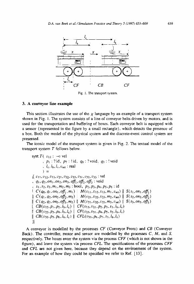
D.A. van Beek et al. /Simulation Practice and Theory 5 (1997) 653-669 659
Fig. 1. The transport system.
3. A conveyor line example
This section illustrates the use of the x language by an example of a transport system shown in Fig. 1. The system consists of a line of conveyor belts driven by motors, and is
used for the transportation and buffering of boxes. Each conveyor belt is equipped with a sensor (represented in the figure by a small rectangle). which detects the presence of
a box. Both the model of the physical system and the discrete-event control system are
presented. The iconic model of the transport system is given in Fig. 2. The textual model of the
transport system T follows below.
syst T( ~11 : 4 vel
, p1 : ?id, p7 : !id, 40 : ? void, 93 : ! void
, let lb, Is, i&t : real
I=
I[ ~11~~12~~13~~219~227~23~~31~~32~~33: vel
, ql,q2,0nl,on2,0n3,0ffl,off2,0ff3 :void SI,Q,S3,“21,W,m3 :bool, p2,p3,p4,p5tpf, :id
i C(q0,4t7w,ofl,ml) II w 41,u12,u13,ml,k) II S(n,m,ofl,)
II C(ql,q2tOn2,0fS22,m2) II M(u21,u22,v23,m2,u,t) II SCs2,on2,&2)
II C(q2,q3,0n3,df3,m3) II M(u31,u32,u33,m3,v,t) II S(s3,on3,@3) Ij C&U12,pl,p;!,~b,k) 11 ~~~~~~~~~~~~~~~~~~~~~~~~~~ (1 CB(WvP3>P4~kvk) 11 CF(v23,v31,P4rP5,S2,Ib,Is) 11 CB(U32>P5>p6,lb,k) )I c~~(u33,P6,~,~3,~b,~,)
II
A conveyor is modelled by the processes CF (Conveyor Front) and CB (Conveyor Back). The controller, motor and sensor are modelled by the processes C, M, and S, respectively. The boxes enter the system via the process CFF (which is not shown in the figure), and leave the system via process CFL. The specifications of the processes CFF and CFL are not given here, because they depend on the environment of the system. For an example of how they could be specified we refer to Ref. [ 131.

660 D.A. van Beek et al./Simulation Practice and Theory 5 (1997) 653-669
fig. 2. Model of the transport system.
The user defined types that are used in different processes are listed below.
type vel = [m/s]
7 pos = [ml id = int
3.1. The model of a motor
The motor is switched on when it receives the value true via channel mj, and is
switched off when it receives the value false. The parameter vSt represents the value of the velocity of the conveyor motor when it is switched on. The velocity u of the motor
is made available to three processes via the continuous channels Ujt, Uj2 and Uj3 (see
Figs. 2 and 3).
proc M( Vjl, Vj2, Vj3 1 -<) vel , mj:?bool , vet : real
I= I[ v : vel , b : boo1
; b := false
1 UjlrUj2*Uj3 --O u
1 [ b-v=v~[ 0 d-v=0
I 1 *[ mj?b ]
II
3.2. The model of a sensor
A sensor is modelled by process S. The control system synchronizes with a sensor by means of the synchronization channels on and o# These are used by the control
D.A. van Beek et al./Simulation Practice and Theory 5 (1997) 653-669 661
system to wait for the sensor to be activated or deactivated. The synchronization on?
in a control process can only take place if the sensor is activated. This is modelled by
‘b ; on ! - skip’ in process S, where skip is the empty statement. Execution of the
statement off? in the control system causes it to block until the sensor is deactivated.
The sensor receives its new state from process CF via channel S. The boolean variable
b denotes the state of the sensor.
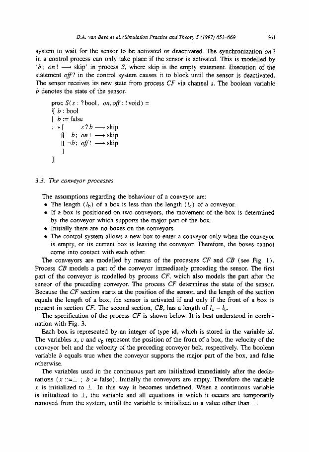
proc S(s : ?bool, on,ofJ: !void) =
I[ b : boo1 1 b :=false
; *I s ? b - skip
i 7:: ’ -skip
Eii - skip
1 II
3.3. The conveyor processes
The assumptions regarding the behaviour of a conveyor are: l The length (Zb) of a box is less than the length (I,) of a conveyor. l If a box is positioned on two conveyors, the movement of the box is determined
by the conveyor which supports the major part of the box. l Initially there are no boxes on the conveyors.
l The control system allows a new box to enter a conveyor only when the conveyor is empty, or its current box is leaving the conveyor. Therefore, the boxes cannot come into contact with each other.
The conveyors are modelled by means of the processes CF and CB (see Fig. 1).
Process CB models a part of the conveyor immediately preceding the sensor. The first part of the conveyor is modelled by process CF, which also models the part after the sensor of the preceding conveyor. The process CF determines the state of the sensor. Because the CF section starts at the position of the sensor, and the length of the section equals the length of a box, the sensor is activated if and only if the front of a box is present in section CF. The second section, CB, has a length of I, - lb.
The specification of the process CF is shown below. It is best understood in combi- nation with Fig. 3.
Each box is represented by an integer of type id, which is stored in the variable id.
The variables X, u and up represent the position of the front of a box, the velocity of the conveyor belt and the velocity of the preceding conveyor belt, respectively. The boolean
variable b equals true when the conveyor supports the major part of the box, and false otherwise.
The variables used in the continuous part are initialized immediately after the decla-
rations (x ::=i ; b := false). Initially the conveyors are empty. Therefore the variable x is initialized to _L. In this way it becomes undefined. When a continuous variable is initialized to I, the variable and all equations in which it occurs are temporarily removed from the system, until the variable is initialized to a value other than _I_.

662 D.A. van Beek et al./Simularion Practice and Theory 5 (1997) 653-669
Fig. 3. Model of a conveyor.
The entry of a box onto the conveyor is modelled by the communication pk ? id. As a result, the sensor is activated (s ! true), and x is initialized to 0. The trajectory of x
is determined by the value of its derivative (x’). This value equals either the velocity up of the preceding conveyor (if b is false) or the velocity u of the conveyor itself
(if b is true), depending on the position of the box. In the discrete-event section, two state-events are used. The first state-event represents the detection that the major part of the box is supported by the conveyor, i.e. V x = I, + i&,_ By subsequently assigning the value true to b, the equation X’ = L: is selected. The second state-event represents the
moment at which the box reaches the process boundary, i.e. V x = I,,_ Consequently the communication pl ! id is executed, the sensor is deactivated (S ! false), and the variable x is reinitialized at 1. From this point on, the position of the box is determined by the
next process.
proc CF( Uia, Ujr : -0 vel , pk:?id, pl:!id, s:!bool
, lb,& : real
I[ n : pas), : 0 : vel , b: bool, id:id ; x ::=_L ; b := false
I &3 -0 up
v;1 +v
i [ 7b - X' = up
II b -x'=u
1 1 *[ pk?id; s!true; b:=false; x::=O
; Vx = 1, + $lb ; b := true ; vx=/b; pl!id; s!falSe; x::=l
I
II
The specification of CB is slightly different from the CF specification. The conditional equation is no longer necessary, because in this process the box is always carried by

D.A. van Beek et al. /Simulation Practice and Theory 5 (1997) 653-669 663
the conveyor itself. The discrete event part is also simplified, because the state of the sensor is not affected by process CB.
proc CB( uj2 : -D vel , pj : ?id, p,,, : !id
, lb,/, : real
)= ([ n : pos, u : vel
, id:id ; x ::=I
/ Vj2 4 V
x1 = v
1 *[ pl?id; x::=O; vx=l,-lb; pm!id; x::=_L]
II
4. The conveyor line control system
The control system is included, because it clarifies the sensor and actuator based interaction between the control system and the conveyors.
4.1. A simplified control strategy
The specification of the control process C follows below (see also Fig. 2). The control strategy is straightforward: new boxes are allowed to enter only when the sensor is not activated, and the conveyor is therefore empty. When the synchronization via qin
succeeds, the motor of the conveyor is switched on (m ! true). The control process then waits until the sensor is activated (on ?), so that the box is at the end of the conveyor.
The process then checks if the next conveyor is ready to receive a box (qoUt !). If this is the case, then the synchronization qout ! . 1s executed. If the next conveyor cannot receive a box within 0.1 seconds, the time-out A 0.1 is executed. As a result the motor is switched off, and the control process waits until the next conveyor can receive a box. Then it
starts the motor. Finally, it waits until the box has left the conveyor (ofs?), before a new box may enter the conveyor.
procC(qi,: ?void, qO,,!void, on,ofJ:?void, m: !bool) =
I[ * [ 9in ? ; m!true; on?
; [ qout ! - skip fl AO.1 -m!false; qout!; m!true
I ; off? 1
II
4.2. A more eflcient control strategy
A more optimal strategy is presented below. In this case, boxes are allowed to enter a conveyor as soon as the box already present on the conveyor has reached the sensor
664 D.A. van Beek et al. /Simulation Practice and Theory 5 (1997) 653-669
(on ?), and is leaving the conveyor. The advantage of this strategy is that there can be two boxes on a conveyor instead of just one, which results in an increased throughput.
Four different states are used in the controher: (i) EMPTY: At first the conveyor is empty, not running, and is able to receive and
transport a box. (ii) RATS (running at sensor) : The conveyor is running with a box that has reached
the sensor. At this stage, the controller tries to send to qout to see if the next conveyor can receive the box. If this is not possible within 0.1 seconds (A 0. 1 ), the motor stops (m ! false) and the controller waits until the next conveyor can receive the box.
(iii) ROUT (running out) : The box can leave the conveyor. When leaving, two events are possible. Either a second box may enter the conveyor (qin ?), or the box leaving the conveyor may clear the detector (of?) before a second box has entered. If a new box has entered first, the control process subsequently waits for the first box to have left the conveyor (og?), and then waits for the second box to reach the detector (on ?) .
(iv) REMPTY (running empty) : If there is no new box within 5 seconds, the motor stops, and the state s becomes EMpTY.
proc C (9in : ?void, qout!void, on,o$: ?void, m: !bool) = I[ s : {EMPTY,ROUT,REMpTY,RATS}
1 s:=EMPTY
; *[ s=EMPlY ; qin? -m!true; ~YZ?; s:=RATS
0 s=RATS ; qout ! - s := ROUT
0 s=RATS ; Ao.1 --+m!false; qout!; m!true; S:=ROm
0 s=ROUT ; qin? -of?; On?; s:=RATS
0 s= ROUT ; off? -s:=REMPTY
[1 s=FEMPTY; qin? -on?; s:=RATS
0 s=REMpTY; A.5 -m!false; s:=EMPTY
I
II
5. Extensions to the conveyor line example
In this section the conveyors are modelled in more detail. Two extensions are pre- sented: a conveyor motor with start-up and shut-down characteristics, and a conveyor line on which the boxes may collide.
5.1. Extensions to the motor
The motor described in the previous section had two states only: on or off. The motor specified below has two additional states: accelerating and decelerating. The variable s stores the state of the motor, it can take on any of the values in the set {STOPPED, ACC, MAX, DEC}. When the motor is switched on, its velocity u rises with a constant acceleration a,[ until the maximum velocity u,[ is reached. The motor process continuously tries to receive a new command from the control system (mj ? b). When the motor receives a new command via channel mj, it first checks the state of the

D.A. van Beek et al. /Simulation Practice and Theory 5 (1997) 653-669 665
Fig. 4. Model of the conveyors with colliding boxes.
motor. If it is turned on and it is not yet at its maximum velocity (b A s + MAX) the state is set to accelerate (S := ACC). If it is turned off and it has not yet stopped
(-b As # STOPPED), the state is set to decelerate. If the state s equals ACC, the process
waits until the motor has achieved its maximum speed (V u = u,~), and subsequently
switches the state to MAX.
proc M( Ujl.Uj2,Cj3 1 -0 vel , mj:?bool
, aset, uset : real I=
I[ u : vel , b : boo1 , s : {STOPPED, ACC, MAX, DEC}
; c ::=o; s := STOPPED
1 Ujl,Cj2,Uj3 4 L:
1 [ s=MAXVs=STOPPED-u’=O
0 s=ACC I
- u = aset
0 s = DEC /
-u =-L&t
mj?b -[ br\s#mx --+s:=ACC
0 Tb A s # STOPPED - s := DEC
1 0 s=ACC; vu=uset -s:=MAX
fl s=DEC; vu=0 -s:=STOPPED
1 II
5.2. Conveyors with colliding boxes
In this section a more accurate model of the conveyors is presented. This model takes
into account the possibility of colliding boxes. If a box enters a conveyor section that contains a box which is not moving, the entering box collides with the box already present. It is assumed, that as a result of a collision the velocity of the entering box becomes equal to the minimum of ( 1) the velocity of the conveyor section by which it is supported and (2) the velocity of the box in front of it.
Only process CBC (Conveyor Back Colliding) is specified. The specification of process CFC is similar. The specification of the process follows below. Fig. 4 shows the process CBC together with the surrounding processes CFC.
666 D.A. van Beek et al./Simulation Practice and Theory 5 (1997) 653-669
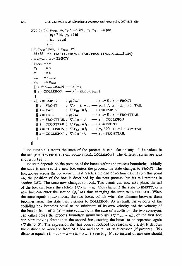
proc CBC( umotor, ul, u, : -0 vel, x1, xm : --o pos , pl:?id, p,:!id
, &,I, : real
I[ X,Xnext fpis, U,hext : k-21 , id : id, s : {EMPTY, FRONT, TAIL, FRONlTAIL, COLLISION}
; X ::=I ; s := EMPTY
I JJmOlOr -0 u
. Xl -0X
3 u1 --ou
1 Xn -0 Xnext 9 urn 4 hext 1 [ s # COLLISION - x’ = u
0 s = COLLISION - x’ = min( u, unext)
1 1 *[ s=EMPTY ; pl ?id - x ::= 0; s := FRONT
IIS = FRONT ; vx=l,-lb -pm!id; x::=I; s:=TAIL
OS =TAIL ; v Xmt = lb -s:=EMP-IY
0 s=TAIL ; pl? id -x::=O; s:=FRONTl?AIL
0 S=FRON?TAIL; Vdist=O - s := COLLISION
/-j S = FRONTTAIL; v Xnext = lb - S := FRONT
0 s=COLLISION; vX,rxt=/b -pm!id; x::=l; s:=TAIL
0 s= COLLISION ; V dist > 0 - s := FRONTTAIL
1 II
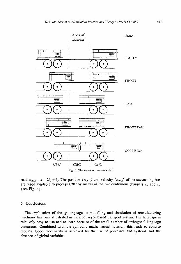
The variable s stores the state of the process, it can take on any of the values in the set {EMPTY, FRONT, TAIL, FRONTTAIL, COLLISION}. The different states are ah0
shown in Fig. 5. The state depends on the position of the boxes within the process boundaries. Initially
the state is EMPTY. If a new box enters the process, the state changes to FRONT. The
box moves across the conveyor until it reaches the end of section CBC. From this point on, the position of the box is described by the next process, but its tail remains in
section CBC. The state now changes to TAIL. Two events can now take place: the tail of the box can leave the section (V xnext = lb) thus changing the state to EMPTY, or a new box can enter the section (pi ? id) thus changing the state to FRON?TW. When the state equals FRoN-ITAIL, the two boxes collide when the distance between them becomes zero. The state then changes to COLLISION. As a result, the velocity of the colliding box becomes equal to the minimum of its own velocity and the velocity of the box in front of it (x’ = min( u, u ,,xt) ) _ In the case of a collision, the two conveyors
can either cross the process boundary simultaneously (V xnext = lb), or the first box can start moving faster than the second box, causin g the boxes to be separated again (V dist > 0). The expression dist has been introduced for reasons of clarity. It denotes the distance between the front of a box and the tail of its successor (if present). This distance equals (I, - lb) - x - (lb - xnext) ( see Fig. 6), so instead of dist one should
D.A. van Beek er al. /Simulation Practice and Theory 5 (1997) 653-669 667
Area of interest
1 1 I ‘/ ,!, ,8/S
,piji’, ;- / B!_
L /
no ; + + : + OCE + CFC : CBC ; CFC
Fig. 5. The states of process CBC.
State
EMPTY
FRONT
TAIL
FRONTTAIL
COLLISION
read Xnext - x - 21b + I,. The position ( nnext) and velocity ( vnext) of the succeeding box are made available to process CBC by means of the two continuous channels x,,, and L’,,, (see Fig. 4).
6. Conclusions
The application of the ,y language to modelling and simulation of manufacturing machines has been illustrated using a conveyor based transport system. The language is relatively easy to use and to learn because of the small number of orthogonal language constructs. Combined with the symbolic mathematical notation, this leads to concise models. Good modularity is achieved by the use of processes and systems and the absence of global variables.

668 D.A. van Beek et al./Simulation Practice and Theory 5 (1997) 653469
CBC I CFC I CBC I CFC
Fig. 6. Conveyors with colliding boxes.
The integration of continuous-time and discrete-event concepts in the language makes
it highly suitable for machine modelling. In the continuous-time parts of the models, positions of moving parts are described by simple DAEs. In order to simplify models, many actions of machines can be abstracted as discrete-event actions. For this purpose, the x language provides CSP-based discrete-event constructs. Changes in the velocity of moving parts can be simplified as discontinuous changes, which are modelled in the discrete-event part of the processes. The crossing of process boundaries by products
is modelled by synchronous communications. Interaction between the continuous-time
and discrete-event parts of processes is achieved by means of assignments to variables occurring in DA&, or by means of the nabla operator in order to synchronize with state
events. The x simulator for the discrete-event part of the language [21] is being used
in a large number of cases. The cases deal with modelling and simulation of complex
discrete-event manufacturing systems, such as production facilities for integrated circuits.
The first version of the x simulator for combined continuous-time / discrete-event systems [ 121 has recently been completed.
The x language can also be used for the specification of control systems, including exception handling [ 6,7 J . Such a control model can be tested by connecting it to a model
of the controlled machines. The sensors and actuators serve as the interface between the controller and the controlled system. The combined system can then be simulated.
In this way, the combined continuous-time / discrete-event approach to modelling and simulation of manufacturing machines can be an important aid for the development of robust machine control systems.
Acknowledgements
We like to thank Ralph Walenbergh for his contribution to the control system specifi- cation. Thanks are also due to the reviewers for their helpful comments on the draft of
this paper.
D.A. van Beek et al. /Simulation Practice and Theory 5 (I 997) 653-669 669
References
[ I ] M. Andersson, Combined object-oriented modelling in Omola, in: Proceedings of the 1992 European Simulation Multiconference, York, 1992, pp. 246-250.
[2] N.W.A. Arends, A systems engineering specification formalism, Ph.D. Thesis, Eindhoven University of
Technology, The Netherlands, 1996.
[3] Speedup user guide, Aspen Technology, Cambridge, 1991.
(41 J. le Bail, H. Alla and R. David, Asymptotic continuous Petri Nets: An efficient approximation of
discrete event systems, in: IEEE International Conference on Robotics and Automation, Nice, 1992, pp.
1050-1056.
[5] P.I. Barton, The modelling and simulation of combined discrete/continuous processes, Ph.D. Thesis,
University of London, 1992.
[6] D.A. van Beek, Exception handlin g in control systems, Ph.D. Thesis, Eindhoven University of
Technology, The Netherlands, 1993.
[7] D.A. van Beek and J.E. Rooda, A new mechanism for exception handling in concurrent control systems,
Eur. J. Control (2) (1996) 88-100.
[ 81 D.A. van Beek, J.E. Rooda and S.H.E Gordijn, A combined continuous-time / discrete-event approach
to modelling and simulation of manufacturing machines, in: Proceedings of the 1995 EUROSIM
Conference, Vienna, 1995, pp. 1029-1034.
[9] R. David and H. Alla, Petri Nets for modeling of dynamic systems: A survey, Automatica 30 (2) ( 1994)
175-202.
[lo] Department of Mathematics Delft University of Technology and Computer Science, Prosim Reference
Manual, Sierenberg en de Gans, Waddinxveen, The Netherlands, 1995.
[ 1 l] H. Elmqvist. Dymola-dynamic modeling language-user’s manual, Dynasim AB, Lund, Sweden, 1994.
[ 121 G. Fabian and P. Janson, Simulator for combined continuous-time / discretexvent models, Final report of
the Postgraduate Programme Software Technology, Eindhoven University of Technology, Stan Acketmans
Institute, The Netherlands, 1996.
[ 131 S.H.F. Gordijn, Combined continuous-time / discrete-event specifications of industrial systems using
the language x, Master’s Thesis, Department of Mechanical Engineering, Eindhoven University of
Technology, The Netherlands, 1995.
[ 141 C.A.R. Hoare, Communicating Sequential Processes, Prentice-Hall, Englewood-Cliffs, 1985.
[ 151 J. Hooman, Specification and Compositional Verification of Real-Time Systems, Springer-Verlag, 1991.
[ 161 B.W. Kemighan and D.M. Ritchie, The C Programming Language (ANSI Standard C) Prentice-Hall,
Englewood Cliffs. 1988.
[ 171 D.L. Kettenis, Issues of parallelization in implementation of the combined simulation language
COSMOS, Ph.D. Thesis, Delft University of Technology, 1994.
[ 181 E.E.L. Mitchell and J.S. Gauthier, Advanced continuous simulation language (ACSL), Simulation 26
(3) (1976) 72-78.
[ 191 J.M. van de Mortel-Fronczak and J.E. Rooda, Application of concurrent programming to specification
of industrial systems, in: Proceedings of the 1995 IFAC Symposium on Information Control Problems
in Manufacturing, Bejing, 1995, pp. 421-426.
[20] J.M. van de Mortel-Fronczak, J.E. Rooda and N.J.M van den Nieuwelaar, Specification of a flexible
manufacturing system using concurrent programming, Concurrent Eng. Res. Appl. 3 (3) (1995) 187-
194. [21] G. Naumoski and W.T.M Albert% The x engine: A fast simulator for systems engineering, Final
report of the Postgraduate Programme Software Technology, Eindhoven University of Technology. Stan
Ackermans Institute, The Netherlands, 1995.
[ 221 C.D. Pegden, R.E. Shannon and R.F? Sadowski, Introduction to Simulation Using SIMAN, McGraw-Hill,
1995.
[23] N. Zerhouni and H. Alla, Dynamic analysis of manufacturing systems using continuous Petri Nets, in: IEEE International Conference on Robotics and Automation, Cincinnati, 1990, pp. 1070-1075.