Discrete and Continuous Probability Distributions.
54
Discrete and Continuous Probability Distributions
-
Upload
coleen-norton -
Category
Documents
-
view
244 -
download
0
Transcript of Discrete and Continuous Probability Distributions.
Discrete and Continuous Probability Distributions

Goals
After completing this session, you should be able to:
Apply the binomial distribution to applied problems Compute probabilities for the Poisson distribution Find probabilities using a normal distribution table
and apply the normal distribution to some biomedical problems
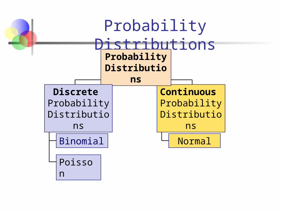
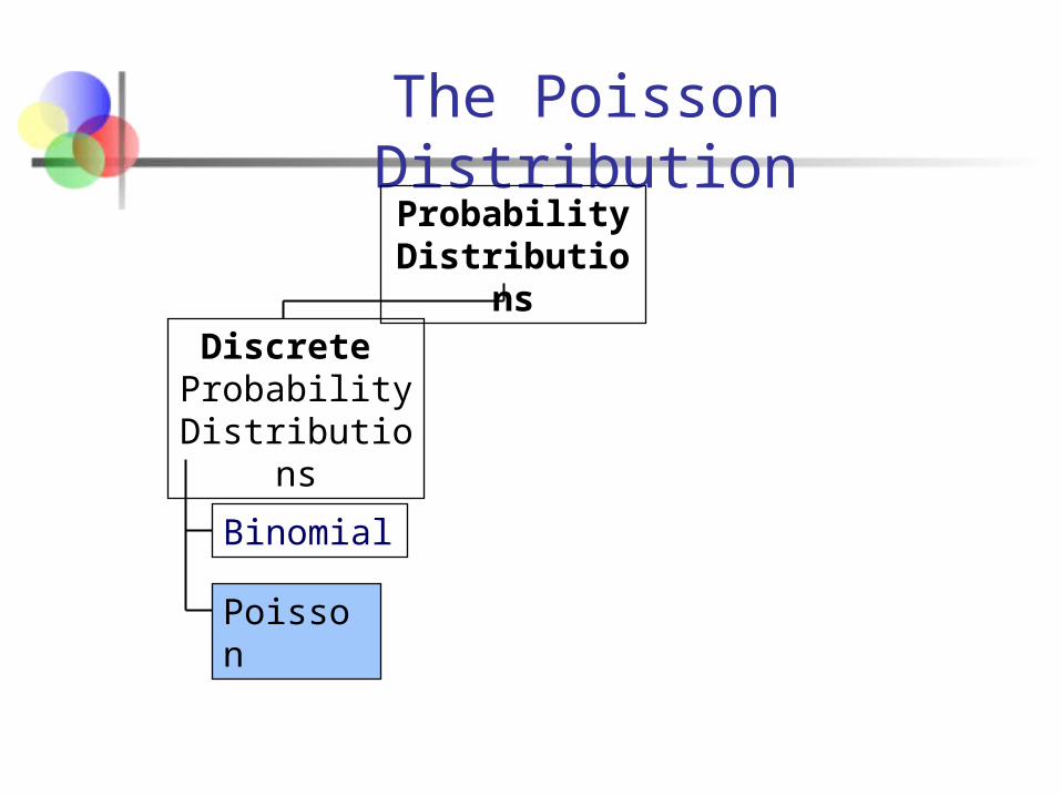
Probability Distributions
Continuous Probability
Distributions
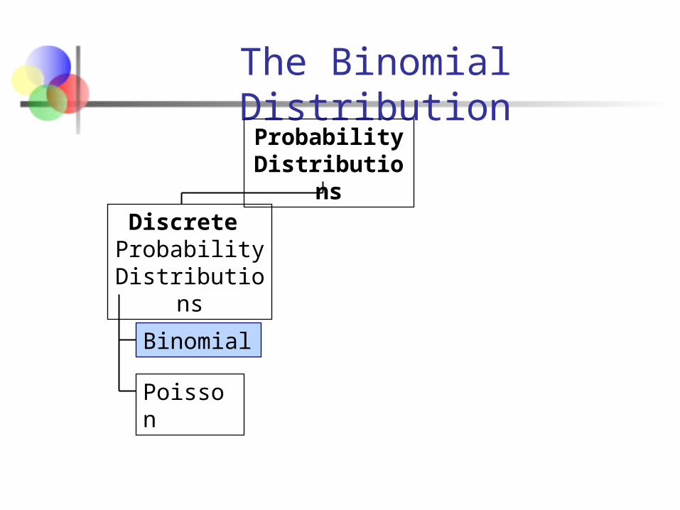
Binomial
Poisson
Probability Distributions
Discrete Probability
Distributions
Normal
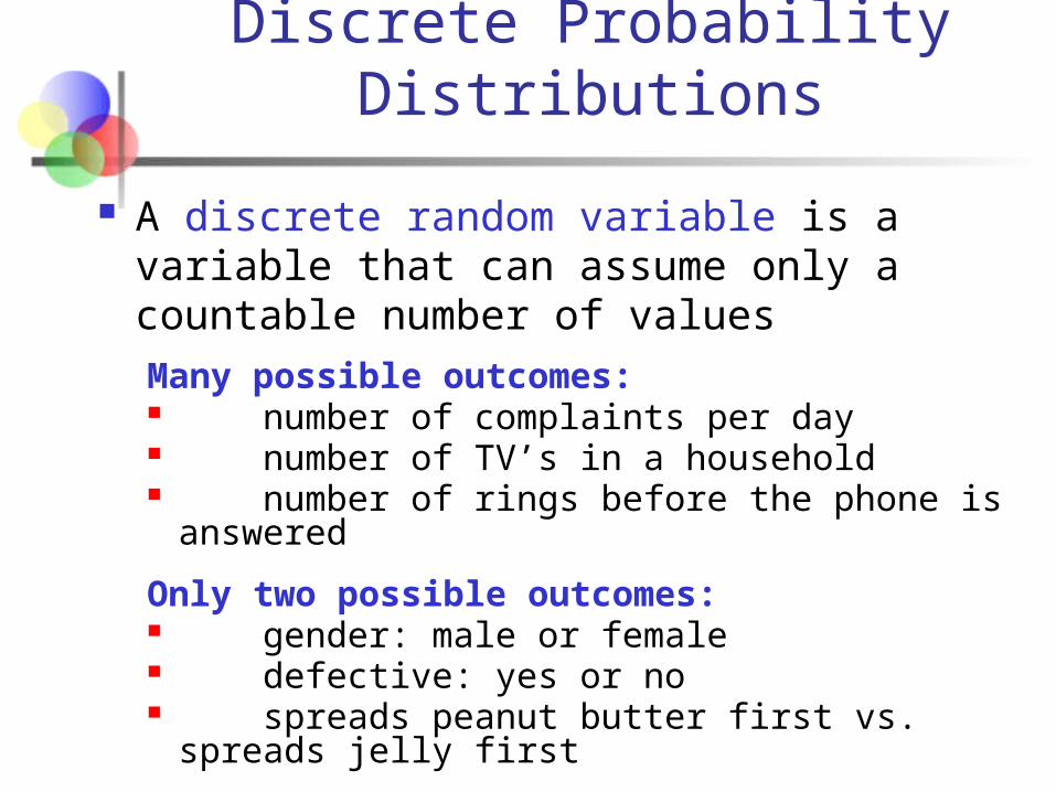
A discrete random variable is a variable that can assume only a countable number of values
Many possible outcomes: number of complaints per day number of TV’s in a household number of rings before the phone is answered
Only two possible outcomes: gender: male or female defective: yes or no spreads peanut butter first vs. spreads jelly first
Discrete Probability Distributions
Continuous Probability Distributions
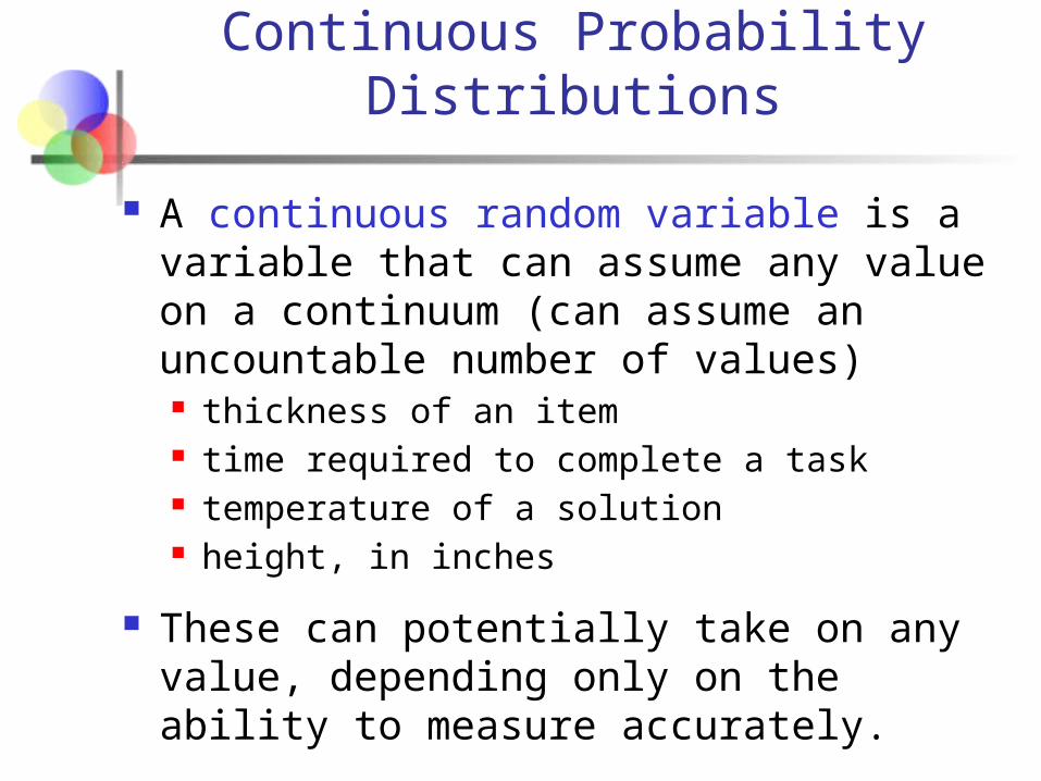
A continuous random variable is a variable that can assume any value on a continuum (can assume an uncountable number of values) thickness of an item time required to complete a task temperature of a solution height, in inches
These can potentially take on any value, depending only on the ability to measure accurately.
The Binomial Distribution
Binomial
Poisson
Probability Distributions
Discrete Probability
Distributions
The Binomial Distribution
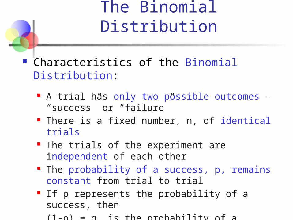
Characteristics of the Binomial Distribution:
A trial has only two possible outcomes – “success” or “failure”
There is a fixed number, n, of identical trials The trials of the experiment are independent of each
other The probability of a success, p, remains constant from
trial to trial If p represents the probability of a success, then
(1-p) = q is the probability of a failure
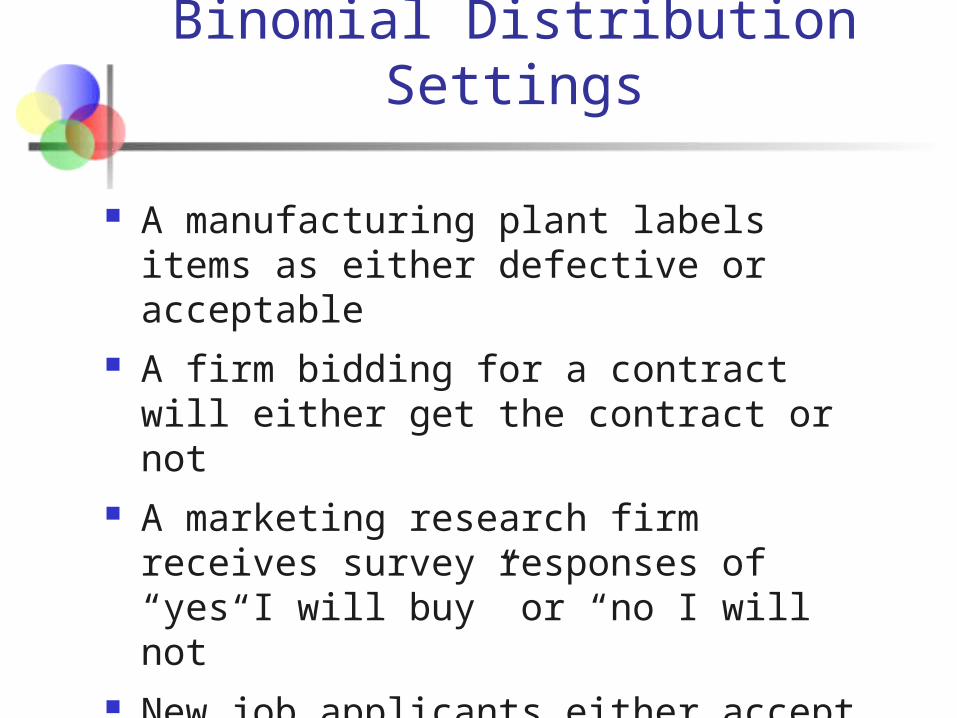
Binomial Distribution Settings
A manufacturing plant labels items as either defective or acceptable
A firm bidding for a contract will either get the contract or not
A marketing research firm receives survey responses of “yes I will buy” or “no I will not”
New job applicants either accept the offer or reject it
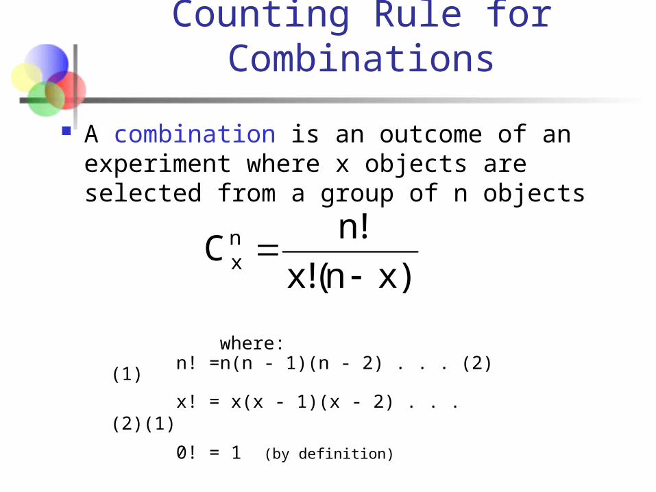
Counting Rule for Combinations
A combination is an outcome of an experiment where x objects are selected from a group of n objects
)!xn(!x
!nCn
x
where:n! =n(n - 1)(n - 2) . . . (2)(1)
x! = x(x - 1)(x - 2) . . . (2)(1)
0! = 1 (by definition)
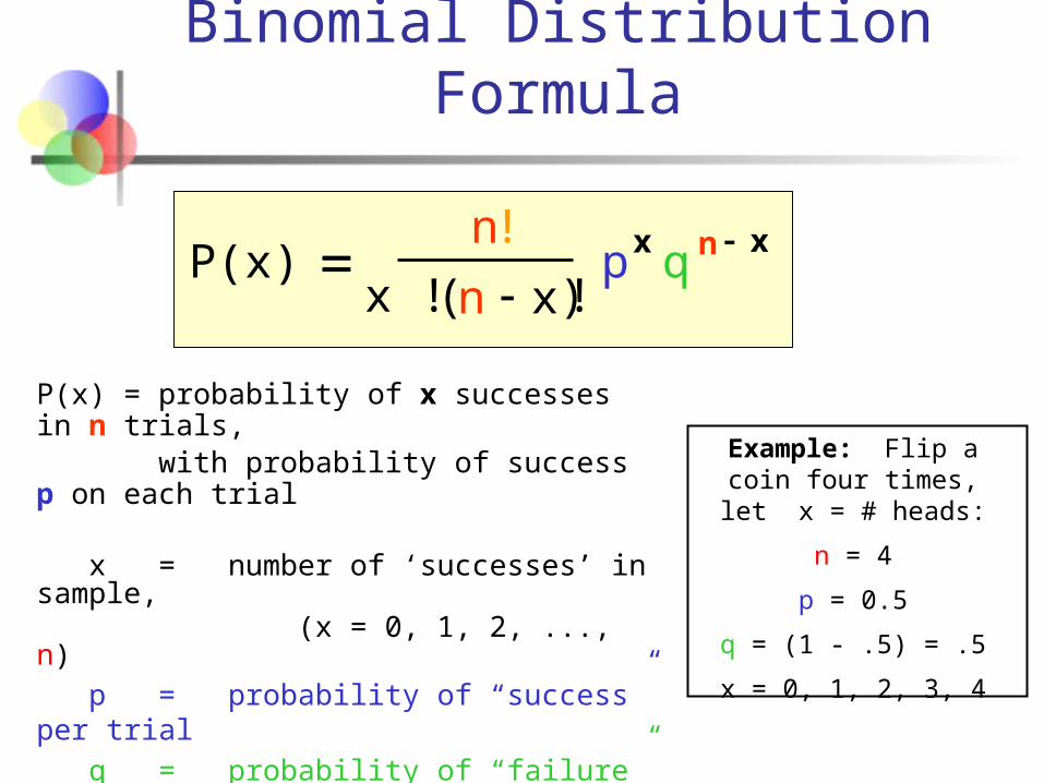
P(x) = probability of x successes in n trials, with probability of success p on each
trial
x = number of ‘successes’ in sample, (x = 0, 1, 2, ..., n) p = probability of “success” per trial
q = probability of “failure” = (1 – p)
n = number of trials (sample size)
P(x)n
x ! n xp qx n x!
( )!=
--
Example: Flip a coin four times, let x = # heads:
n = 4
p = 0.5
q = (1 - .5) = .5
x = 0, 1, 2, 3, 4
Binomial Distribution Formula
n = 5 p = 0.1
n = 5 p = 0.5
Mean
0.2.4.6
0 1 2 3 4 5
X
P(X)
.2
.4
.6
0 1 2 3 4 5
X
P(X)
0
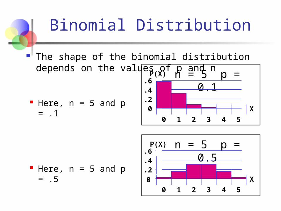
Binomial Distribution
The shape of the binomial distribution depends on the values of p and n
Here, n = 5 and p = .1
Here, n = 5 and p = .5
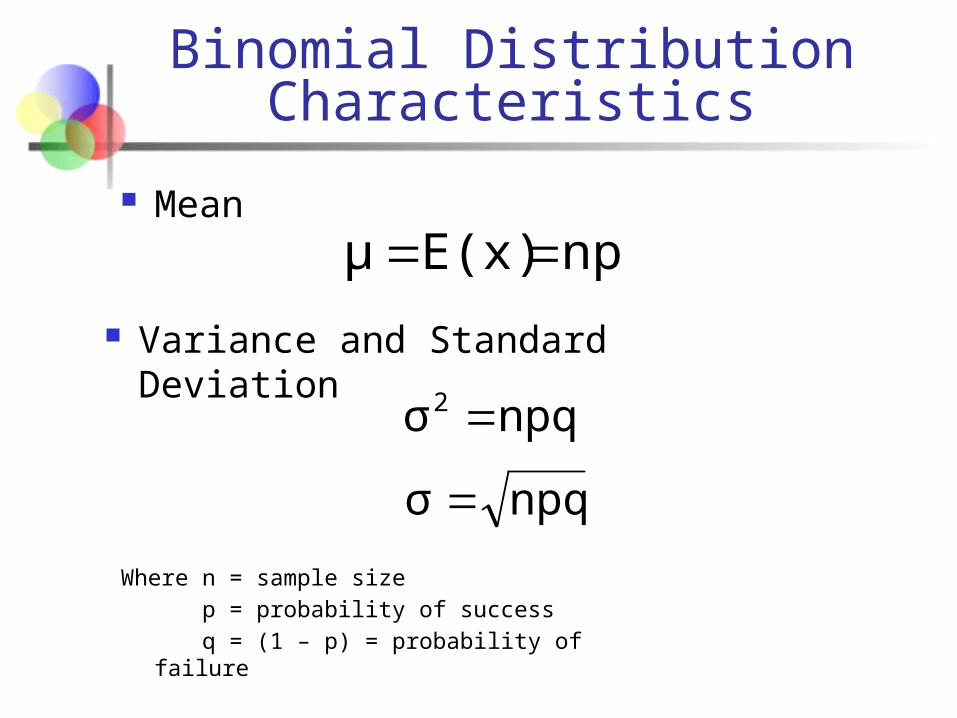
Binomial Distribution Characteristics
Mean
Variance and Standard Deviation
npE(x)μ
npqσ2
npqσ
Where n = sample size
p = probability of success
q = (1 – p) = probability of failure
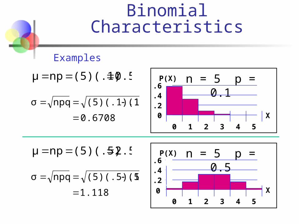
n = 5 p = 0.1
n = 5 p = 0.5
Mean
0.2.4.6
0 1 2 3 4 5
X
P(X)
.2
.4
.6
0 1 2 3 4 5
X
P(X)
0
0.5(5)(.1)npμ
0.6708
.1)(5)(.1)(1npqσ
2.5(5)(.5)npμ
1.118
.5)(5)(.5)(1npqσ
Binomial Characteristics
Examples
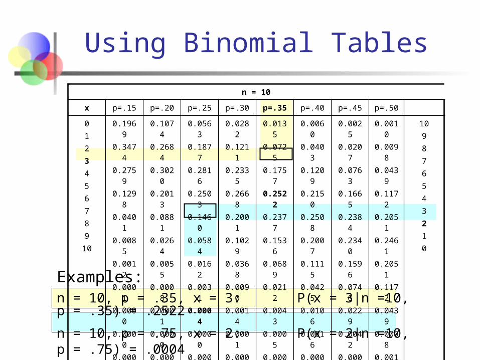
Using Binomial Tables
n = 10
x p=.15 p=.20 p=.25 p=.30 p=.35 p=.40 p=.45 p=.50
0123456789
10
0.19690.34740.27590.12980.04010.00850.00120.00010.00000.00000.0000
0.10740.26840.30200.20130.08810.02640.00550.00080.00010.00000.0000
0.05630.18770.28160.25030.14600.05840.01620.00310.00040.00000.0000
0.02820.12110.23350.26680.20010.10290.03680.00900.00140.00010.0000
0.01350.07250.17570.25220.23770.15360.06890.02120.00430.00050.0000
0.00600.04030.12090.21500.25080.20070.11150.04250.01060.00160.0001
0.00250.02070.07630.16650.23840.23400.15960.07460.02290.00420.0003
0.00100.00980.04390.11720.20510.24610.20510.11720.04390.00980.0010
109876543210
p=.85 p=.80 p=.75 p=.70 p=.65 p=.60 p=.55 p=.50 x
Examples: n = 10, p = .35, x = 3: P(x = 3|n =10, p = .35) = .2522
n = 10, p = .75, x = 2: P(x = 2|n =10, p = .75) = .0004

Using Excel Select More Functions / BINOMDIST
Press then select more
Function
select BINOMDIST
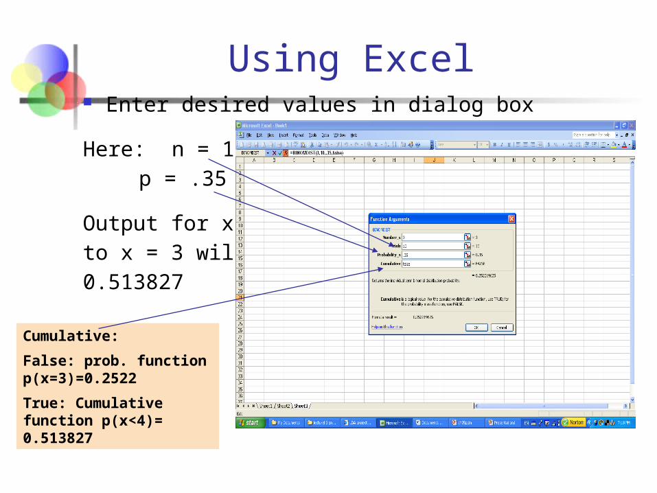
Using Excel Enter desired values in dialog box
Here: n = 10
p = .35
Output for x = 0
to x = 3 will be
0.513827
Cumulative:
False: prob. function p(x=3)=0.2522
True: Cumulative function p(x<4)= 0.513827

P(x = 3 | n = 10, p = .35) = .2522
Output
P(x > 5 | n = 10, p = .35) = .0949
The Poisson Distribution
Binomial
Poisson
Probability Distributions
Discrete Probability
Distributions
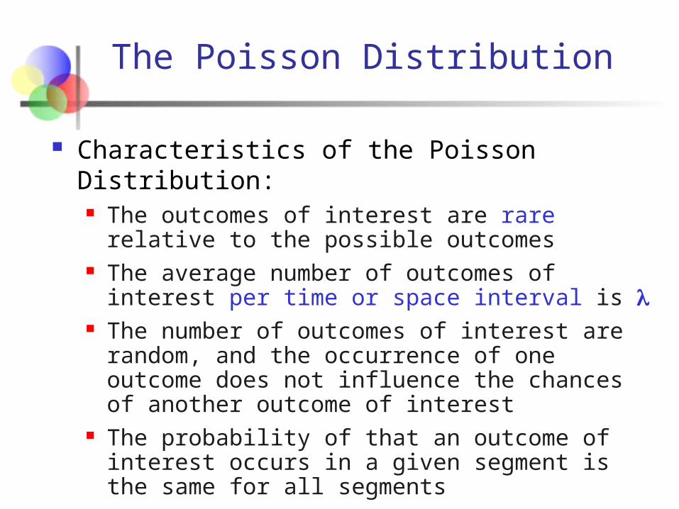
The Poisson Distribution
Characteristics of the Poisson Distribution: The outcomes of interest are rare relative to the
possible outcomes The average number of outcomes of interest per time
or space interval is The number of outcomes of interest are random, and
the occurrence of one outcome does not influence the chances of another outcome of interest
The probability of that an outcome of interest occurs in a given segment is the same for all segments

Poisson Distribution Formula
where:
t = size of the segment of interest
x = number of successes in segment of interest
= expected number of successes in a segment of unit size
e = base of the natural logarithm system (2.71828...)
!x
e)t()x(P
tx
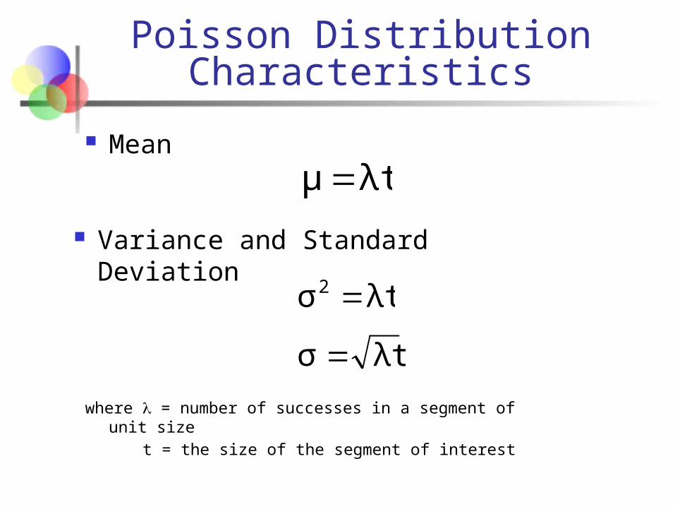
Poisson Distribution Characteristics
Mean
Variance and Standard Deviation
λtμ
λtσ2
λtσ where = number of successes in a segment of unit size
t = the size of the segment of interest
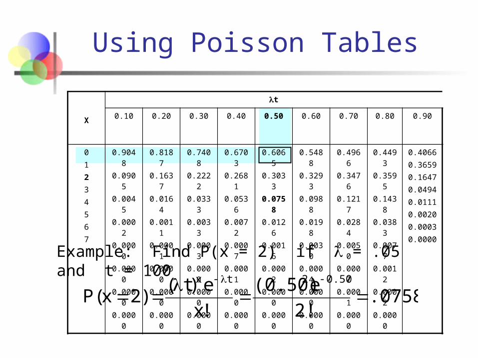
Using Poisson Tables
X
t
0.10 0.20 0.30 0.40 0.50 0.60 0.70 0.80 0.90
01234567
0.90480.09050.00450.00020.00000.00000.00000.0000
0.81870.16370.01640.00110.00010.00000.00000.0000
0.74080.22220.03330.00330.00030.00000.00000.0000
0.67030.26810.05360.00720.00070.00010.00000.0000
0.60650.30330.07580.01260.00160.00020.00000.0000
0.54880.32930.09880.01980.00300.00040.00000.0000
0.49660.34760.12170.02840.00500.00070.00010.0000
0.44930.35950.14380.03830.00770.00120.00020.0000
0.40660.36590.16470.04940.01110.00200.00030.0000
Example: Find P(x = 2) if = .05 and t = 100
.07582!
e(0.50)
!x
e)t()2x(P
0.502tx
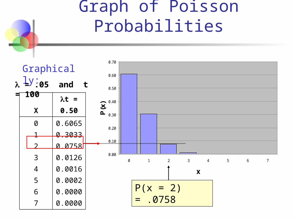
Graph of Poisson Probabilities
0.00
0.10
0.20
0.30
0.40
0.50
0.60
0.70
0 1 2 3 4 5 6 7
x
P(x
)X
t =0.50
01234567
0.60650.30330.07580.01260.00160.00020.00000.0000 P(x = 2) = .0758
Graphically:
= .05 and t = 100
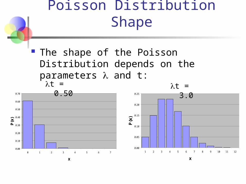
Poisson Distribution Shape
The shape of the Poisson Distribution depends on the parameters and t:
0.00
0.05
0.10
0.15
0.20
0.25
1 2 3 4 5 6 7 8 9 10 11 12
x
P(x
)
0.00
0.10
0.20
0.30
0.40
0.50
0.60
0.70
0 1 2 3 4 5 6 7
x
P(x
)
t = 0.50 t = 3.0
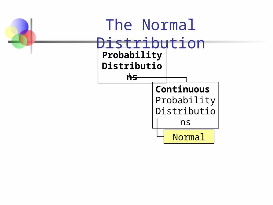
The Normal Distribution
Continuous Probability
Distributions
Probability Distributions
Normal

The Normal Distribution
‘Bell Shaped’ Symmetrical Mean, Median and Mode
are EqualLocation is determined by the mean, μ
Spread is determined by the standard deviation, σ
The random variable has an infinite theoretical range: + to
Mean = Median = Mode
x
f(x)
μ
σ

By varying the parameters μ and σ, we obtain different normal distributions
Many Normal Distributions
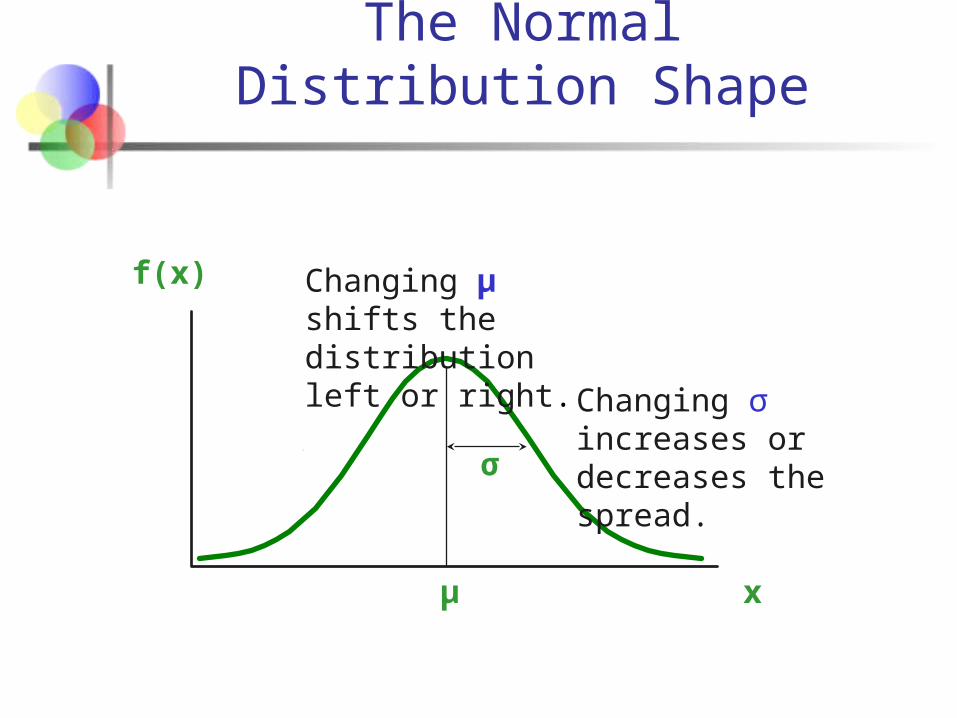
The Normal Distribution Shape
x
f(x)
μ
σ
Changing μ shifts the distribution left or right.
Changing σ increases or decreases the spread.

Finding Normal Probabilities
Probability is the area under thecurve!
a b x
f(x) P a x b( )
Probability is measured by the area under the curve
f(x)
xμ
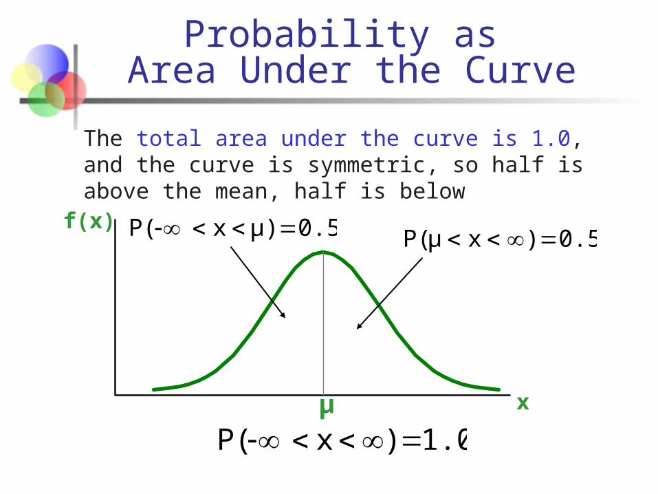
Probability as Area Under the Curve
0.50.5
The total area under the curve is 1.0, and the curve is symmetric, so half is above the mean, half is below
1.0)xP(
0.5)xP(μ 0.5μ)xP(
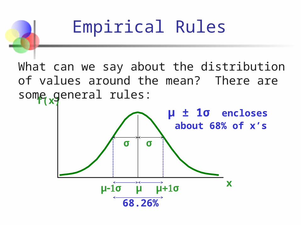
Empirical Rules
μ ± 1σ encloses about 68% of x’s
f(x)
xμ μ+1σμ-1σ
What can we say about the distribution of values around the mean? There are some general rules:
σσ
68.26%
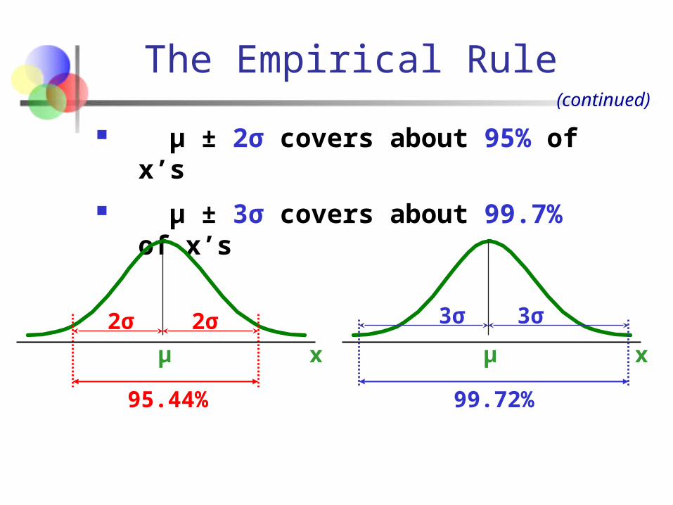
The Empirical Rule
μ ± 2σ covers about 95% of x’s
μ ± 3σ covers about 99.7% of x’s
xμ
2σ 2σ
xμ
3σ 3σ
95.44% 99.72%
(continued)
Importance of the Rule
If a value is about 2 or more standard deviations away from the mean in a normal distribution, then it is far from the mean
The chance that a value that far or farther away from the mean is highly unlikely, given that particular mean and standard deviation
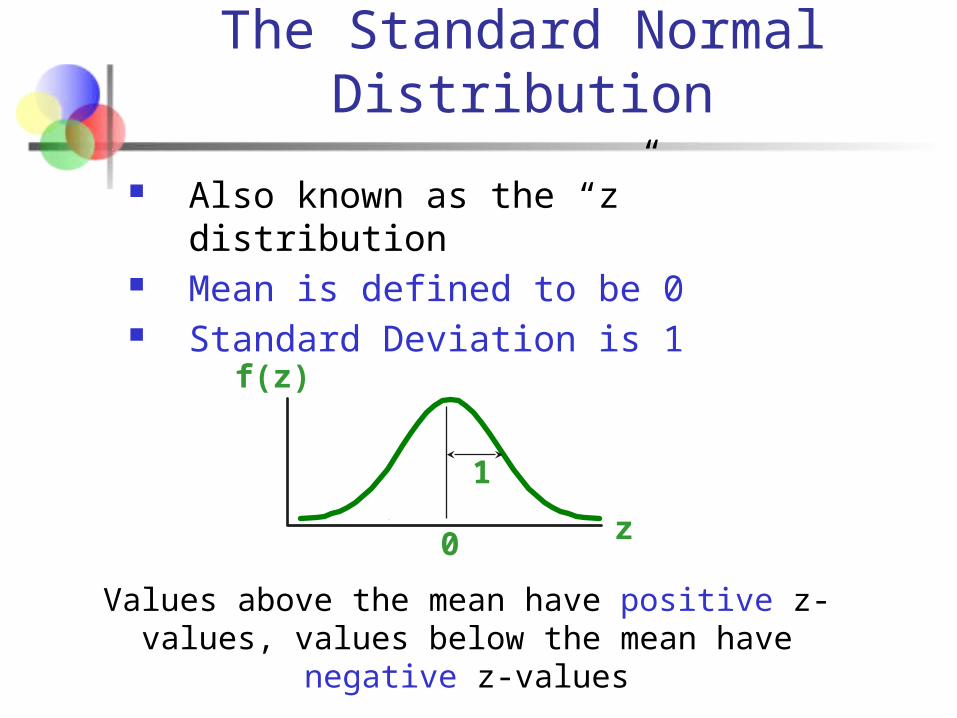
The Standard Normal Distribution
Also known as the “z” distribution Mean is defined to be 0 Standard Deviation is 1
z
f(z)
0
1
Values above the mean have positive z-values, values below the mean have negative z-values
The Standard Normal
Any normal distribution (with any mean and standard deviation combination) can be transformed into the standard normal distribution (z)
Need to transform x units into z units

Translation to the Standard Normal Distribution
Translate from x to the standard normal (the “z” distribution) by subtracting the mean of x and dividing by its standard deviation:
σ
μxz
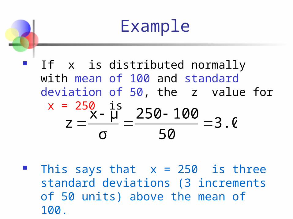
Example
If x is distributed normally with mean of 100 and standard deviation of 50, the z value for x = 250 is
This says that x = 250 is three standard deviations (3 increments of 50 units) above the mean of 100.
3.050
100250
σ
μxz
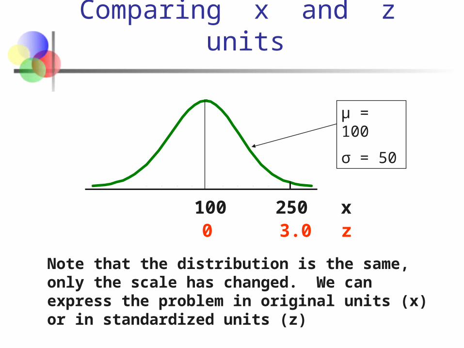
Comparing x and z units
z100
3.00250 x
Note that the distribution is the same, only the scale has changed. We can express the problem in original units (x) or in standardized units (z)
μ = 100
σ = 50
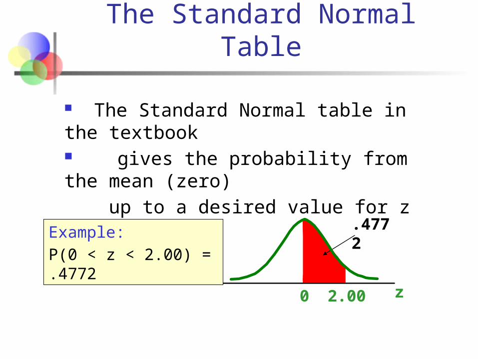
The Standard Normal Table
The Standard Normal table in the textbook
gives the probability from the mean (zero)
up to a desired value for z
z0 2.00
.4772Example:
P(0 < z < 2.00) = .4772

The Standard Normal Table
The value within the table gives the probability from z = 0 up to the desired z value
z 0.00 0.01 0.02 …
0.1
0.2
.4772
2.0P(0 < z < 2.00) = .4772
The row shows the value of z to the first decimal point
The column gives the value of z to the second decimal point
2.0
.
.
.
(continued)

General Procedure for Finding Probabilities
Draw the normal curve for the problem in terms of x
Translate x-values to z-values
Use the Standard Normal Table
To find P(a < x < b) when x is distributed normally:
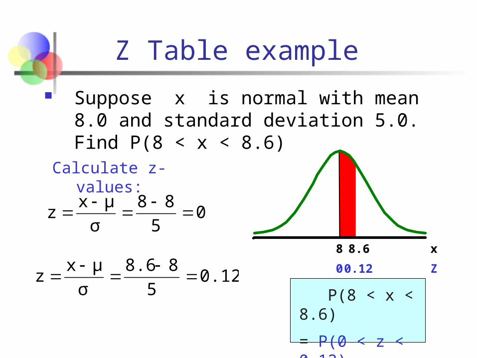
Z Table example
Suppose x is normal with mean 8.0 and standard deviation 5.0. Find P(8 < x < 8.6)
P(8 < x < 8.6)
= P(0 < z < 0.12)
Z0.12 0
x8.6 8
05
88
σ
μxz
0.125
88.6
σ
μxz
Calculate z-values:

Z Table example Suppose x is normal with mean 8.0 and
standard deviation 5.0. Find P(8 < x < 8.6)
P(0 < z < 0.12)
z0.12 0x8.6 8
P(8 < x < 8.6)
m = 8 = 5
m = 0 = 1
(continued)

Z
0.12
z .00 .01
0.0 .0000 .0040 .0080
.0398 .0438
0.2 .0793 .0832 .0871
0.3 .1179 .1217 .1255
Solution: Finding P(0 < z < 0.12)
.0478.02
0.1 .0478
Standard Normal Probability Table (Portion)
0.00
= P(0 < z < 0.12)P(8 < x < 8.6)
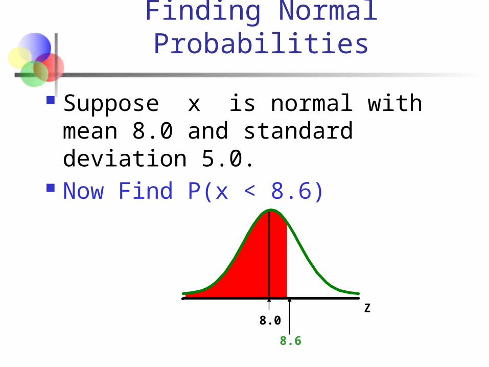
Finding Normal Probabilities
Suppose x is normal with mean 8.0 and standard deviation 5.0.
Now Find P(x < 8.6)
Z
8.6
8.0
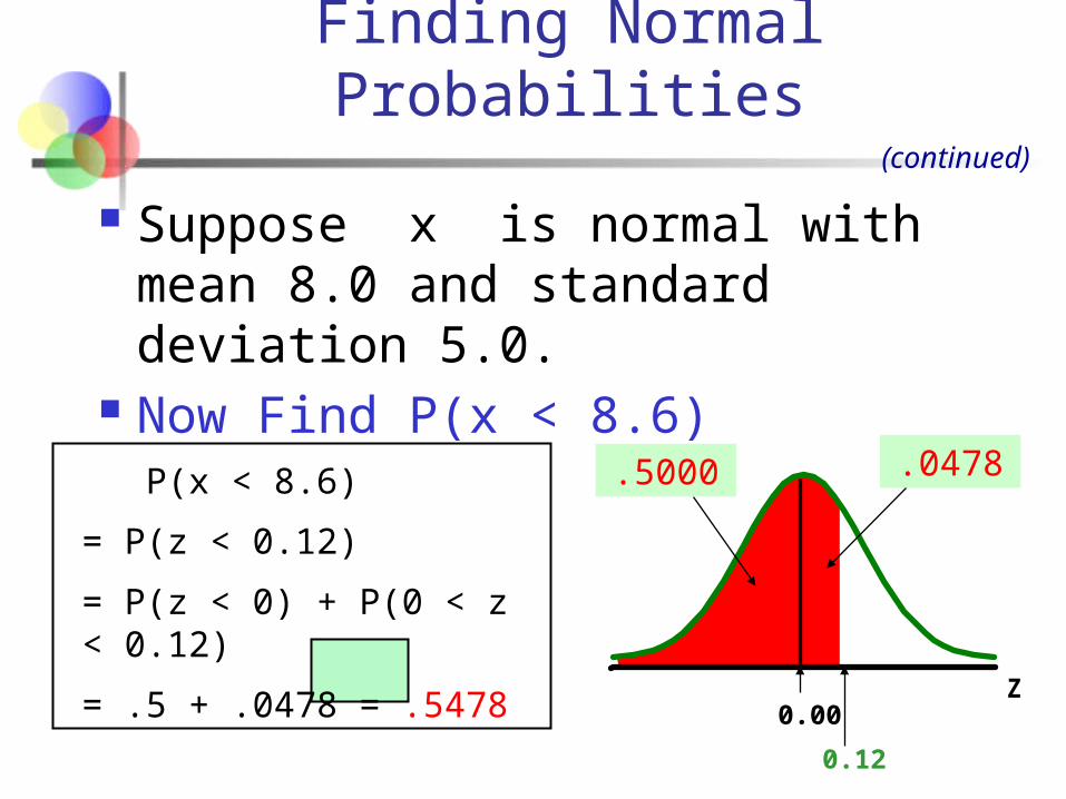
Finding Normal Probabilities
Suppose x is normal with mean 8.0 and standard deviation 5.0.
Now Find P(x < 8.6)
(continued)
Z
0.12
.0478
0.00
.5000 P(x < 8.6)
= P(z < 0.12)
= P(z < 0) + P(0 < z < 0.12)
= .5 + .0478 = .5478
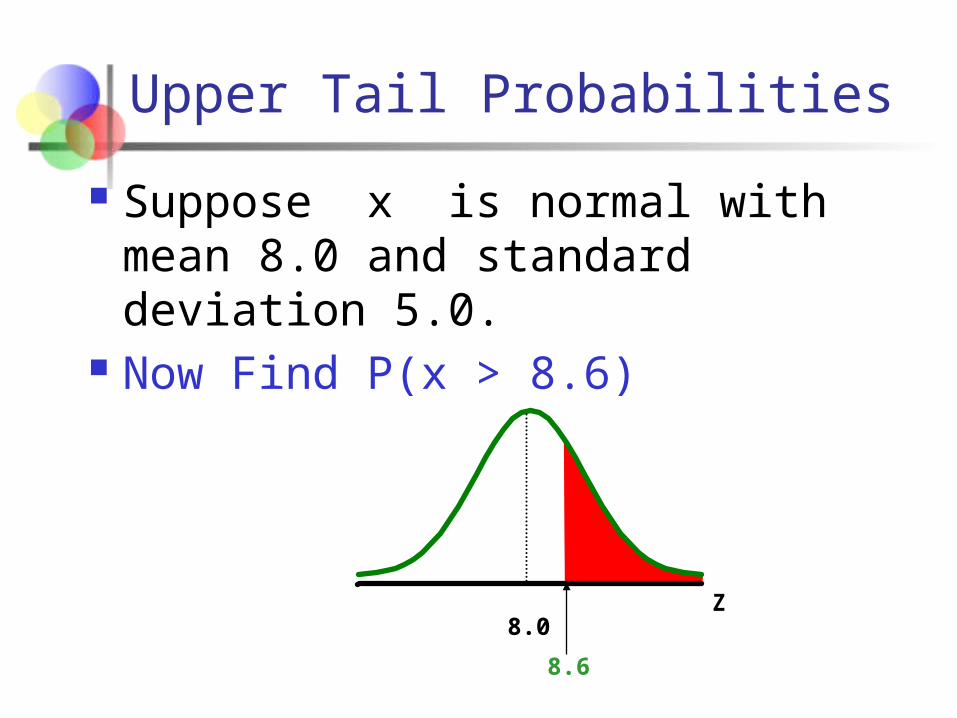
Upper Tail Probabilities
Suppose x is normal with mean 8.0 and standard deviation 5.0.
Now Find P(x > 8.6)
Z
8.6
8.0
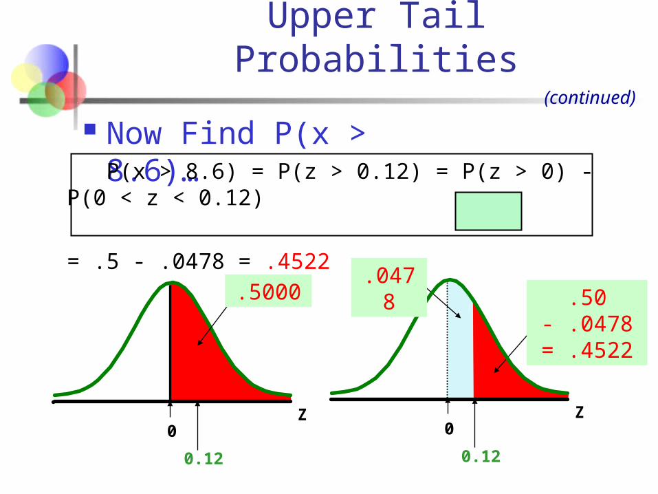
Now Find P(x > 8.6)…(continued)
Z
0.12
0Z
0.12
.0478
0
.5000 .50 - .0478 = .4522
P(x > 8.6) = P(z > 0.12) = P(z > 0) - P(0 < z < 0.12)
= .5 - .0478 = .4522
Upper Tail Probabilities
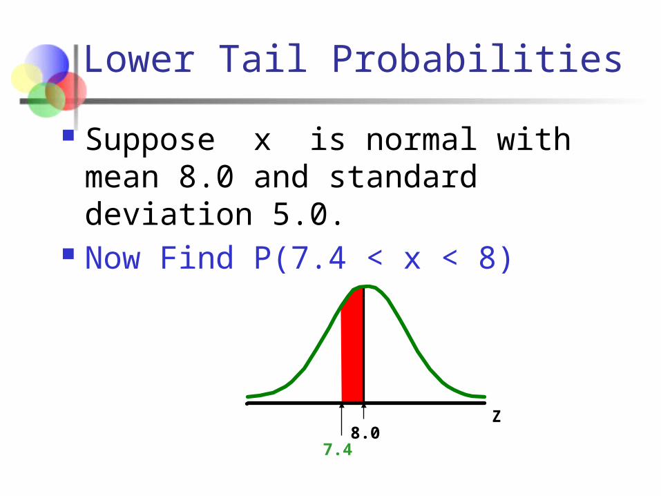
Lower Tail Probabilities
Suppose x is normal with mean 8.0 and standard deviation 5.0.
Now Find P(7.4 < x < 8)
Z
7.48.0
Lower Tail Probabilities
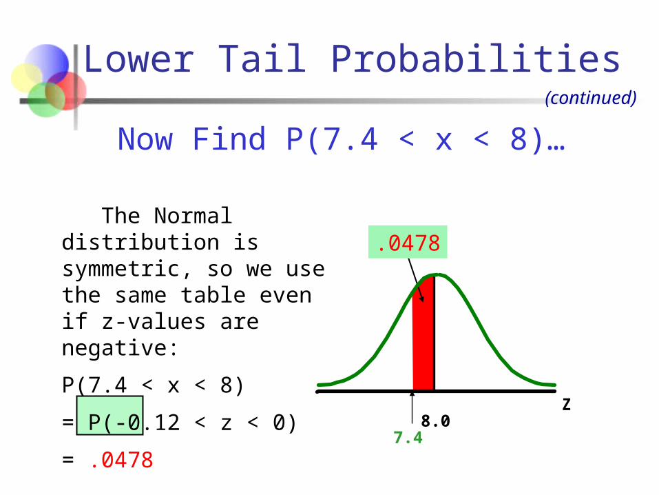
Now Find P(7.4 < x < 8)…
Z
7.48.0
The Normal distribution is symmetric, so we use the same table even if z-values are negative:
P(7.4 < x < 8)
= P(-0.12 < z < 0)
= .0478
(continued)
.0478
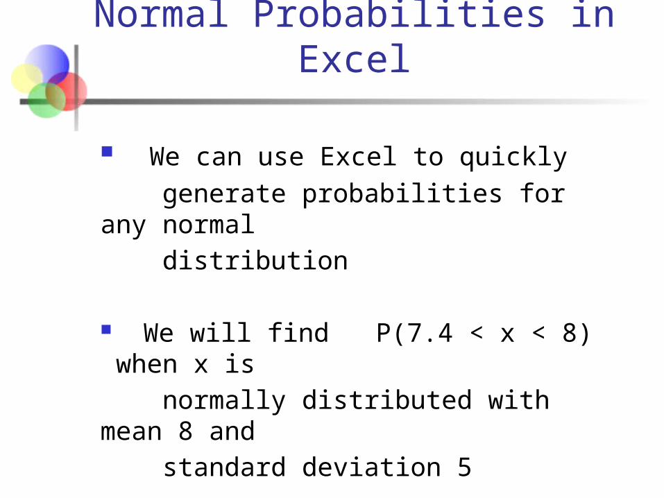
Normal Probabilities in Excel
We can use Excel to quickly
generate probabilities for any normal
distribution
We will find P(7.4 < x < 8) when x is
normally distributed with mean 8 and
standard deviation 5
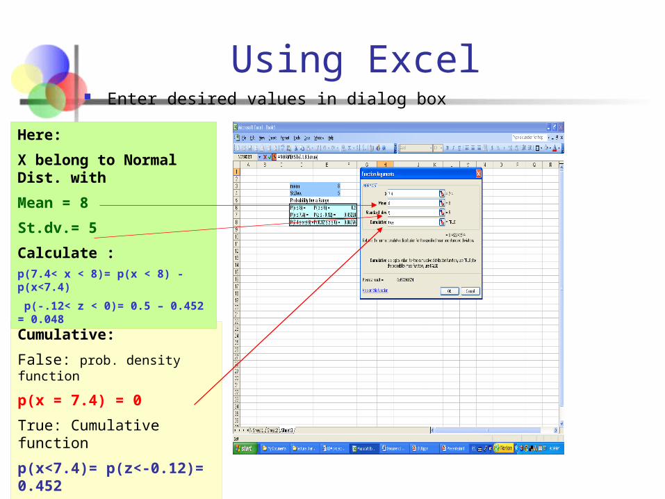
Using Excel Enter desired values in dialog box
Cumulative:
False: prob. density function
p(x = 7.4) = 0
True: Cumulative function
p(x<7.4)= p(z<-0.12)= 0.452
p(x < 8)= p(z < 0) = 0. 5
Here:
X belong to Normal Dist. with
Mean = 8
St.dv.= 5
Calculate : p(7.4< x < 8)= p(x < 8) - p(x<7.4)
p(-.12< z < 0)= 0.5 – 0.452 = 0.048
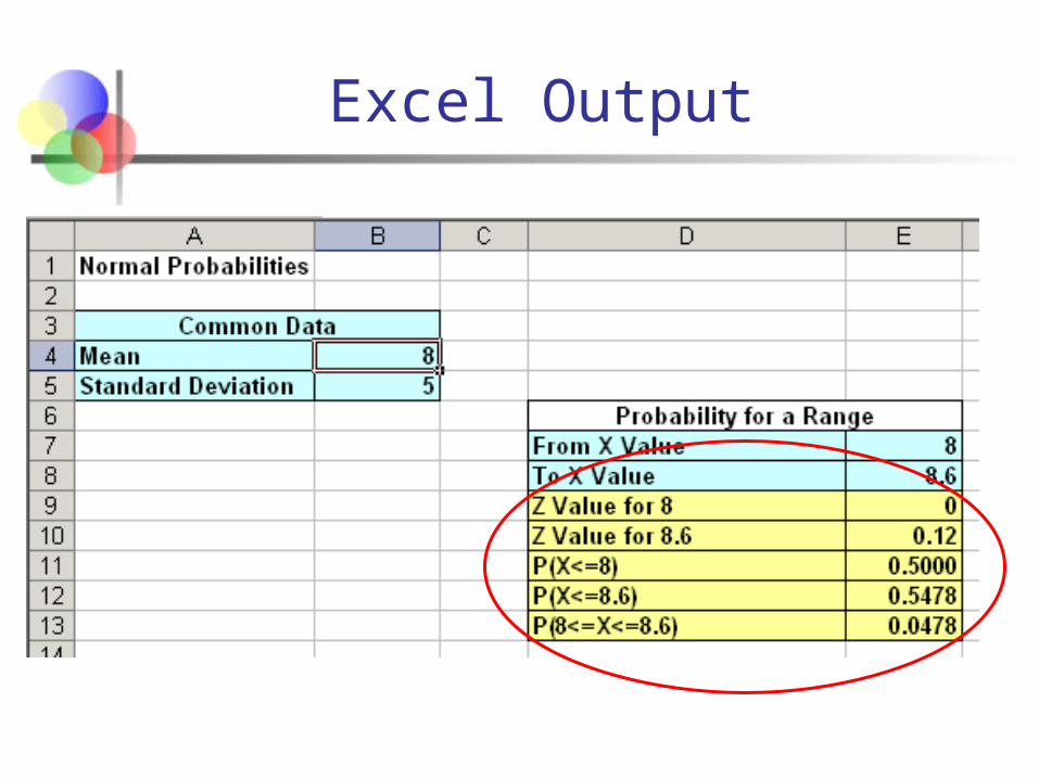
Excel Output
Summary
Reviewed key discrete distributions binomial and Poisson
Reviewed key continuous distribution normal
Found probabilities using formulas and tables
Recognized when to apply different distributions
Applied distributions to decision problems