10/4/2017

NG

WA

WH

ITE

PAPE

R

Modeling groundwater in the subsurface environment gives us a view and insight of what cannot be easily seen nor readily observed. The U.S. Geological Survey anticipates future modeling demands will be greater, especially addressing multi-disciplinary factors and applied to landscape-level science as scientific questions and resource issues become more complex. The National Ground Water Association (NGWA) determined that to further support the many interests affected by groundwater, it should mobilize its members to collaborate to improve groundwater modeling and its application. On April 14, 2016, NGWA convened nearly 40 prominent groundwater modelers to form the Groundwater Modeling Advisory Panel (GMAP).

The goal of GMAP is to advance the state of groundwater modeling through cooperative information exchange and outreach to groundwater professionals. The GMAP objectives are to address groundwate modeling practice and to research questions and identify alternative/best techniques and responses. GMAP members intend to provide the scientists and engineers involved in groundwater modeling applications—professionals and interested members of the public—with our collective understanding of the subject matter and observations for consideration in professional practice. We decided not to develop standards, as our members saw the modeling field on a path of continuing and rapid evolution.

The members of GMAP identified 33 topics of interest and categorized them into five groups for development. Each group had eight to 15 members and two Co-Leads who facilitated discussions and

Integrated Surface Water- Groundwater ModelingPreface for Groundwater Modeling Advisory Panel White Papers

PrecipitationPrecipitation

2

organized preparation of modeling practice white papers. The five initial topic groups were: field complexity, stepwise/analytical element modeling, uncertainty in modeling, model applications, and integrated groundwater/surface water modeling. The papers are written as discussion documents to be updated.

The groups met monthly, distributed document development responsibilities, drafted sections of papers, completed their selected modeling practice topic papers, and conducted peer review from approximately June 2016 to June 2017. The NGWA Board of Directors approved the papers in October 2017.

The papers address questions of:• How should decision makers consider groundwater modeling in project development and solution?• How should the complexity of the subsurface be considered in developing groundwater models?• What considerations should be made in moving from simple to more complex model development?• How can uncertainty be included in modeling to inform decisions for groundwater supply and

remediation?• What approaches can be followed to address interaction of groundwater and surface water in

decisions?GMAP members believe sharing their knowledge and experience will assist both long-time practitioners

and newly-graduated modelers in applying their skills and expertise. The Advisory Panel also hopes modelers will bring other questions forward for consideration and development in future groundwater modeling practice white papers. Future discussions and papers are already planned.

Integrated Surface Water–Groundwater ModelingThe individuals who gave of their time and expertise on this paper were:

Authors Reviewers

Miln Harvey Eve Kuniansky Peter Mock Jaco Nel Jill Van Dyke Jeff Davis Jim Finegan Sean Kosinski Jack Hermance Charlie McLane

David Bean

IntroductionProcess-based, physically representative mathematical models are now able to simulate the transport of

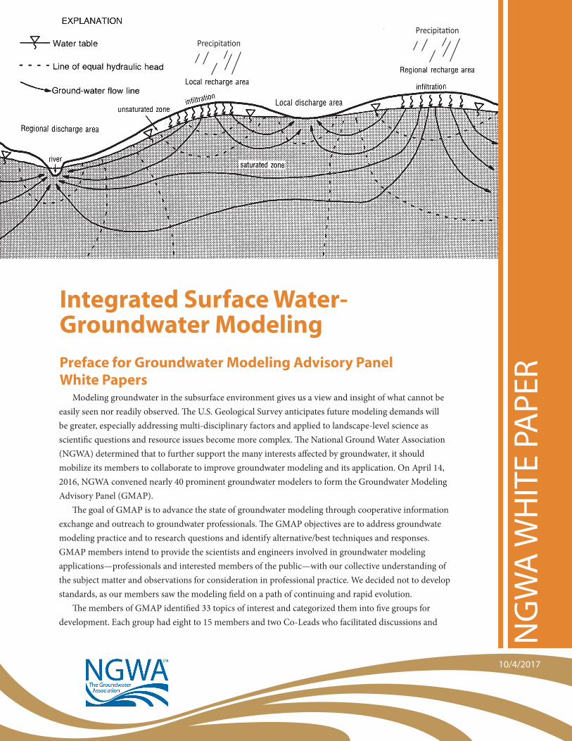
water throughout the atmosphere, across the land-atmosphere boundary, and throughout the subsurface as saturated-unsaturated groundwater flow. The paradigm that has been historically referred to by hydrologists as the “water cycle” has now captured the attention of a much wider audience than that of traditional groundwater and surface water hydrology. The protection and sustainability of water in the environment, particularly in the critical zones of surface vegetation, soil and bedrock, affects not only water supplied to local users, but also the long-term stewardship of the larger landscape even impacting the weather and climate (NRC 2001). The surface landscape—soil moisture, vegetation, heat capacity, land surface slope, surface radiance and reflectance, etc.—is often a controlling factor in creating weather systems on all scales, as well as playing a fundamental role in the partitioning of precipitation into evapotranspiration, runoff, and infiltration.

The transdisciplinary science of hydrology is particularly well represented in the development and application of integrated surface water–groundwater models (Fatichi et al. 2016). Over the years hydrological science has evolved in response to individual project needs, the community, and the respective missions of

3

local, state, and national agencies, of which the United States Geological Survey (USGS), the Department of Agriculture (USDA), the Department of Energy (USDOE), the National Oceanic and Atmospheric Administration (NOAA), the Environmental Protection Agency (USEPA), and the National Science Foundation (NSF) are only a few. On the international scale, scientists in the Global Energy and Water Cycle Exchanges Project (GEWEX) and the World Climate Research Programme (WCRP) are increasingly interested in the coupling of groundwater to basin-scale surface flow through dynamical surface-subsurface interactions, directly through the hyporheic zone or indirectly through unsaturated bi-directional flow in the vadose zone. The proper simulation of these processes in local weather models, and the aggregation of their detailed behaviors to global-scale climate models, is essential (Maxwell et al. 2014).

While large-scale, complex hydrologic models are capable of simulating integrated surface and subsurface flow, results show the best agreement for simpler test cases with more complicated settings is somewhat dependent on the detailed physical representations of particular processes and/or numerical algorithms used for their solutions (Maxwell et al. 2014). In spite of significant progress over the last five decades, Paniconi and Putti (2015) argue that many challenges persist, as analysts try to maintain physical and numerical consistencies in parameterizing and merging multiple interacting linear and non-linear processes across a wide range of scales of the overall system. Fatichi et al. (2016) assert that, for certain classes of problems, these comprehensive, process-based models are most appropriate, but must be used with care. They caution that even though such computational algorithms have been developed to a high level of functionality, the practical application of these types of models often depends on complex or poorly known boundary conditions, local hydrogeology, and initial conditions. The purpose of this paper is to present a balanced assessment of these viewpoints from the perspective of a larger community of users and stakeholders.

Scope of this ReportIntegrated surface water–groundwater models are tools that provide us the opportunity to better simulate

the hydrologic cycle at a local scale or on a catchment level. However, the decision to use an integrated surface water–groundwater model should be based on the level of detail project principals believe is needed to represent the hydrology of the project site to meet study objectives. The decision should also consider the adequacy of the database of information needed to parameterize the model. Whether existing data are sufficient, or additional data will be required, the decision is constrained by factors that include, but are not limited to, the physical hydrologic processes that affect the site, the role of landscapes and hydroclimate in parameterizing the system, the computer modeling codes that are available, and how these codes represent the hydrologic processes in simulating the flow of water through the site.

The objective of this paper is to discuss these issues to provide a better understanding of the place of integrated surface water–groundwater modeling within the realm of groundwater analysis. It was developed by a working group of the National Ground Water Association (NGWA) Groundwater Modeling Advisory Panel (GMAP) to advance the state of groundwater modeling through cooperative information exchange and outreach to groundwater professionals. As such, it is intended to provide those involved in groundwater modeling applications—professionals as well as interested members of the public—with our collective understanding of the subject matter and observations for consideration in professional practice.

BackgroundThe hydrologic cycle describes the continuous movement of water above, on, through, and below the

ground surface (Winter et al. 1998). Traditionally, the analysis of water resources has focused on surface water and groundwater as separate systems. However, because the hydrologic cycle spans the interface at land surface between these systems, hydrologic analysis is an interdisciplinary science that includes

4

hydrologists who normally assess surface water systems, and hydrogeologists who normally assess groundwater systems. In the development of a conceptual site model there is always crossover in water resource analysis beginning with a background analysis of the hydroclimatology (i.e., the interaction between the atmosphere, surface water bodies, and the ground surface environment) in the study area. For example, when completing a hydrogeological assessment of a study site it is important to compile and summarize precipitation measurements, to assess infiltration rates, to estimate groundwater discharge to surface water, to take surface water samples, and to estimate surface water flows in order to develop a better understanding of the water balance of the site. Similarly, when completing a hydrological assessment of a subwatershed it is important to assess baseflow discharge to streams, to install monitoring wells and take groundwater level measurements to assess the location of the water table, and to take groundwater samples to understand water quality impacts on the surface water system. More and more, water resources analysis is becoming an integrated assessment of hydrologic conditions that involves hydrologists, hydrogeologists, and engineers.

Integrated surface water–groundwater models provide an alternative to the traditional modeling of surface water and groundwater environments that, historically, have been considered as separate analyses (Paniconi and Putti 2015; Fatichi et al. 2016). The models that are commonly used to assess the surficial hydrologic environment are classified as surface water models, but these models need to address the groundwater environment as a component, or reservoir, of the hydrologic cycle to more accurately represent flows within the system. The models that are commonly used to assess the environment below land surface are classified as groundwater models, but these models need to address the surface water (and atmospheric) environment as a boundary condition for groundwater flow. It is becoming more common to model these two environments using an integrated approach.

Three commonly-used methodologies that integrate surface water models and groundwater models to better simulate surface water–groundwater interaction include: (1) manually-linked modeling, (2) coupled modeling, and (3) fully-integrated modeling. Descriptions of the models referred to herein are provided later in this paper.

Manually-linked modeling (e.g., MODFLOW/SWMM, MODFLOW/SWAT) is conceptually the easiest, as separate surface water and groundwater models are set up and simulated independently and calibrated to common observation data. Coupled modeling (e.g., GSFLOW, which combines MODFLOW and PRMS) integrates the separate regions of the hydrologic and hydrogeologic systems and simulates each system through boundary condition links using iterative matrix solution methods. Fully-integrated modeling (e.g., HydroGeoSphere, MIKE SHE, CATHY, ParFlow) uses a globally-integrated approach to simultaneously solve the governing equations of surface water flow (i.e., the Saint Venant equations which describe unsteady flow on the land surface) and groundwater flow (i.e., the Richards equation which describes unsteady flow through a variably-saturated porous medium).

The following four sections discuss some of the issues associated with the general process of integrated surface water–groundwater modeling. Information related to modeling codes that are capable of addressing one of more to the three levels of integration is provided in a later section titled “Computer Modeling Codes and the Hydrologic Processes Represented.”

The Physical Processes Affecting Surface Water–Groundwater InteractionThe physical processes that govern the interaction between surface water and groundwater are

dominated primarily by the physiography (land-surface form, geology, and the elevation of the water table) and climate (precipitation and evapotranspiration) of the area under study (Winter 2000). The characterization of these processes are described in detail in several papers that are widely available

5

(Markstrom et al. 2008; Maxwell et al. 2014; Paniconi and Putti 2015; Fatichi et al. 2016). Five factors that dominate the movement of water between surface water and groundwater regimes include: (1) the infiltration/exfiltration characteristics of surface materials, (2) the location and elevation of surface water relative to groundwater, (3) climate, (4) the hydraulic characteristics of the beds underlying surface water bodies, and( 5) the hyporheic zone, for which a recently growing field of study focuses on the very small-scale water exchanges in, and beneath, the beds of flowing streams.

Zones of significant interaction between surface water and groundwater include wetlands, streambeds, hyporheic zones, coastal areas, karst terrain, surface water retention/infiltration ponds, and dewatering sites. Numerical modeling focuses on depicting water flow through these zones, with differences in the modeling based on the physical characteristics of the media, and the spatial and temporal scale of the project. Heterogeneities in the geological material under the surface water body can cause the location and rate of exchange with groundwater to vary significantly over short distances. The unit rate of water exchange (i.e., the flux of water) between surface water and groundwater is a function of surface water stage, the conductance of the bed underlying the surface water body, and the hydraulic conductivity of the underlying vadose zone or aquifer. The horizontal and vertical hydraulic conductivity of the streambed can vary by several orders of magnitude because of the variability of streambed sediments.

The hyporheic zone is one of the more difficult of these zones to characterize. Hyporheic exchange is the process of water exchange between surface water and groundwater across the bed of streams and rivers. Variations in stream slope, streambed sediments, and the hydraulic gradient between surface water and groundwater can result in a hyporheic zone that is several feet in depth below the stream and many hundreds of feet wide. For example, the flow of water from the stream into, and out of, sand or gravel bars provides for a filtering and modification of water chemistry (and heat) that has implications for a wide variety of organisms that inhabit this zone. Because the hyporheic zone is typically close to ground surface, it is also subject to evapotranspiration. All of these processes can be modeled, and each of them should be considered in developing the conceptual model of the site, as they will shape the approach you take in developing the numerical surface water–groundwater flow model.

The Role of a Conceptual ModelProperly establishing the framework for a particular surface water–groundwater application is important

because it defines the purpose of the modeling study, and establishes the audience for the modeling results, which can help inform decisions on the part of the modeler regarding the required level of model sophistication. Once the purpose of the model has been identified, a conceptual model should be developed for the project site. The conceptual site model is an illustrative representation of relevant site features, surface and subsurface conditions, and the hydrologic boundaries that control surface water–groundwater interaction at the site. This interaction can be presented in many forms, which is dictated by the complexity of the site, the physical processes described in the previous section, the type and amount of data that are available to characterize surface water and groundwater conditions, and the requirements of the model application. Because of the complexity of surface water and groundwater interactions over multiple spatial and temporal scales, the conceptual model should be developed in an iterative process that starts with a simple model and progresses through continual refinement as new information is gathered throughout the life-cycle of the project. The level of detail in the conceptual model should match the complexity of site conditions, the availability of high-quality data, and knowledge of the hydrologic processes that drive flow through the site. Thus, this level of detail should be just complex enough to provide the numerical model with sufficient detail to simulate results that answer the questions being asked about the hydrology of the site and adequately meet the objectives of the project study.

6

The level of detail in the conceptual model is also a function of the level of experience of the numerical modeler. Stand-alone groundwater modeling, which can be used to address simple study objectives, requires a simplified characterization of a study area, and can be completed by modelers with a wide range of experience. However, integrated surface water–groundwater modeling requires more in-depth site characterization involving a greater number of parameters and a wider array of data. A review of data gaps at project initiation may provide help in determining the type of modeling that can be done or the costs involved in developing or generating data to fill in the data gaps. A project may start using groundwater modeling with the most readily available data, generate results, and then determine whether the project objectives have been, or are being, addressed by the current model, or whether adjustments in the modeling approach are needed.

Finally, the level of detail in the conceptual model may change if the modeling objectives change. Often a model addresses a single objective or specific question about site conditions, such as: “What is the magnitude of groundwater flux to a river boundary that significantly aids in the design of a groundwater capture system?” A groundwater model can adequately answer this question. But, as the project progresses other objectives may arise as the level of understanding increases about the capabilities of the numerical model, such as answering the question: “How does a reduction in baseflow discharge to the river affect surface water flows and stormwater management design?” This new type of objective may require a change in model type and level of complexity of the conceptual model to accommodate the analysis of more complex surface water–groundwater interactions.

[For further perspective on considering complexity in, and incremental approaches to, groundwater model development, please refer to the NGWA Groundwater Modeling Advisory Panel papers “A Decision Framework for Minimum Levels of Model Complexity” and “A Stepwise Approach to Groundwater Modeling.”]

The Type and Availability of DataEach modeling code has specific data requirements. After the conceptual model has been developed, the

next step in the modeling process is to review appropriate model codes that can generate solutions that meet project objectives. If a coupled or fully-integrated surface water–groundwater model is chosen over groundwater modeling alone, the type and complexity of the data that is needed increases. Groundwater models like MODFLOW require data about layer surface elevations, the distribution of hydrogeological parameters (hydraulic conductivity, storage, and initial heads), and the distribution and time variability of hydrologic boundary conditions (recharge, wells, rivers, lakes, wetlands, springs, seeps, etc.). Integrated surface water–groundwater models like GSFLOW required additional information such as detailed topography, stream flow measurements, stream channel characteristics, climate information (solar radiation, air temperature, wind, detailed precipitation data, etc.), bathymetry, soil data, land cover, etc. Clearly, the data requirements for integrated surface water–groundwater models are much more complicated and the development of such numerical models is more involved.

Because of the importance of basing the modeling process on a realistic view of the physical attributes of a field site, early project planning decisions are needed with respect to the feasibility and cost effectiveness of obtaining additional site data. The efficacy of a modeling outcome depends greatly on the quality of information the modeler has about the physical properties of the site. Obviously, the nature of water-bearing formations is essential, and whether local aquifers are confined or unconfined. The infiltration capacity of the soil, lateral variations in the elevation of the water table, thickness and texture of the overburden, and hydraulic properties of underlying bedrock are clearly essential types of information needed to start a modeling project. Data required for these complex models may be available from a variety of organizations (geological associations, well drillers, municipalities, state and federal governments, etc.); however, data

7

availability can be highly variable depending on the location of the project site and the format of the data. If certain requisite data are not already available, selected field surveys might be required, which might include direct-push probing the overburden, installation of test wells and acquisition of core samples, and perhaps shallow geophysical surveys such as resistivity, seismic results, ground penetrating radar (GPR), electromagnetics, magnetics and/or gravity. A combination of two or more of these geophysical tools usually minimizes the ambiguity often associated with the use of any single tool.

The Role of Landscapes and the Hydroclimate in Parameterizing Integrated Surface Water–Groundwater Models

The range of parameters for integrated surface water–groundwater modeling should reflect the environments to be modeled. Hydroclimatological and landscape metrics incorporated in these models are a function of the physical setting, which could include:

1. Assessing the quality and production capacity of potable groundwater supplies 2. Characterizing streamflow generation and loss 3. Informing geotechnical design of structures concerning potential groundwater and surface

water flows 4. Optimizing agricultural management and production 5. Understanding the processes associated with runoff of agricultural nutrients and pesticides and the

subsequent pollution of surface water, groundwater, and ultimately estuaries, bays, and oceans. In the future, cycling of the Earth’s surface conditions to the atmosphere will become increasingly

important to regional and global meteorological and climate model predictions. The factors described below contribute to the cycling of those conditions and, therefore, to model design.

Precipitation. For the purposes here, the driving factor and primary input for water introduced into the groundwater system is precipitation from either rainfall or snowfall. To properly represent the consequences of this, the location and volume of precipitation must be known along with the characteristics of the land surface (surface soil and its vertical profile; land cover and its spatial and temporal variability; local land slope and/or roughness), which are all required to capture the scale with which vertical infiltration partitions with surface runoff. The intensity, duration, and frequency (IDF) of rainfall, which is a common concern of meteorological hydrology, is becoming a core interest in hydrogeology. In this regard, modelers need to determine, based on project objectives, whether historical or real-time data are needed. A primary question to ask is: ”What level of detail, in space and time, is needed for these parameters to represent the respective modeling period, whether in the past, present or future?” Gauge data can be complemented by weather radar and satellite rainfall estimates (SRFEs). SRFEs from low-Earth orbiting and geosynchronous satellites are critical for providing qualitative detail on the day-by-day spatial and temporal distributions of rainfall at the storm-event level. SRFEs can also provide quantitative detail on precipitation patterns when aggregated at decadal (10-day) or longer time intervals, and lateral scale dimensions of 25 km and greater. Meteorologists consider SRFE precipitation metrics to be reliable on monthly time scales and spatial scales of 100 km × 100 km (1° × 1°) for most regions of the globe, except the high polar region. A database of decreasing quality can be constructed back-in-time to at least the 1980s. Currently, SRFE products for some areas of the globe are at spatial scales of 10 km (even down to 4 km) and temporal scales of one day (even down to 3 hours). While not particularly accurate, such data may be essential for simulating the forcing of integrated surface water–groundwater models for convective thunderstorms, which typically have lateral dimensions of less than 10 km and durations of less than one day. Even broad frontal storm systems, and singular events like hurricanes, may require the modeler to consider the spatial and temporal texture of rainfall only available through SRFE data, or in some cases weather radar.

Snow. Where snow accumulates, the factors affecting snow accumulation, ripening, and melting require

8

an appreciation of the data types and accuracy relevant to snow hydrology. Snow forms a significant recharge mechanism because it provides for longer availability of water that can contribute to aquifer recharge.

Land Cover. State and federal agencies in the United States have very useful land cover data. Satellites provide regular, bi-weekly, or more frequent updates of vegetation cover for the mid-latitudes on a global scale at a 250 m × 250 m resolution. At less regular intervals, land cover is available at 30 m resolution, or better.

Elevation. Elevation is an essential aspect of the landscape for hydrological analyses, and the quality of any particular data needs to be assessed in the context of how it will be used. The partitioning of rainfall between infiltration and surface or subsurface lateral runoff will depend greatly on local land surface gradients. The local slope is difficult to capture from digital elevation models (DEMs) unless the primary elevation data are of very high quality, which cannot be guaranteed in many parts of the world.

Soil Moisture. Another hydroclimate factor to consider is antecedent moisture condition (AMC), which is important in predicting the initial infiltration of rainfall. The AMC varies continuously in time across the landscape, making it a challenging factor to characterize. Other related meteorological factors such as temperature, humidity, wind, and incident solar radiation and cloud cover, which along with plant cover are critical determinants for evapotranspiration of water from the Earth’s surface.

Model Design Planning. Critical to planning the design of a model is to ask: “At what level of accuracy, and at what spatial and temporal scale are these landscape and hydroclimate factors required?” Also, “Are they available on the field site or from adjacent observation stations or might they be provided from satellite remote sensing data?” The decision to proceed with constructing an integrated surface water–groundwater model needs to consider the availability of adequate hydroclimate data, from where it might be derived, and the very character of the spatial and temporal variability of the hydroclimate forcing terms on the scale and duration of the project being considered. Some models will be retrospective, and need past data, perhaps historical data from significantly before the specific period of interest. Other models will be prospective, looking perhaps decades or centuries into the future. Clearly, the demands for the type of hydroclimate data needed for each respective application will be different, with a resulting difference in the expected reliability of the required database, and hence a difference in the degree of confidence one has in the expected outcomes of the modeling exercise vs. the effort and cost of implementing such a model.

Computer Modeling Codes and the Hydrologic Processes RepresentedA number of modeling codes can be used to simulate integrated surface water–groundwater interaction.

Each of these codes represents the physical processes of the hydrologic cycle in a specific way. As a result, a thorough understanding of how the physical processes drive water through a study site is essential to choose the most appropriate code for simulating surface water–groundwater interaction at the site. The computer code should be viewed as a tool that can be used to answer specific questions about a site, but only with a comprehensive understanding of site hydrology.

Integrated surface water–groundwater models can be divided into three types which include linked, coupled, and fully-integrated models.

Linked models run separate simulations of surface water flows and groundwater flows with separate modeling codes and, as an additional, separate process, can impose the results of one model as boundary conditions on the other.

Coupled models run surface water and groundwater models with separate solution processes (two or more separate matrix solutions) in one model simulation, and iteratively and mutually adjust the boundary conditions of each where they have common interfaces during the model simulation.

9

Fully-integrated models run a single simulation that solves both surface water stage and groundwater heads as part of one solution process (a single matrix of combined equations).

Coupled and fully-integrated models represent the forefront of integrated surface water–groundwater modeling.

Maxwell et al. (2014) present a classification scheme for how the interactions between surface water and groundwater are numerically accomplished at the interfaces in integrated surface water–groundwater models:

• Asynchronous linking: lagging the dependent variables (i.e., states) so that governing equations can be solved separately and not at the same time

• Sequential iteration: a time-splitting scheme in which the lagged dependent variables are used to define a functional iteration until convergence

• Globally implicit: assembling all dependent variables in a single, non-linear system of equations.Applying asynchronous linking or sequential iteration leads to coupled models; assembly as a

globally implicit matrix leads to a fully-integrated model. The models discussed herein enforce pressure and flux continuity at the interface between the surface and subsurface domain. It is more challenging to enforce continuity of momentum (and therefore force) at the interface (Maxwell et al. 2014). Enforcement of momentum was not found in the information for the models described herein.

Many NGWA groundwater professionals will be familiar with the use of MODFLOW as a groundwater model, so a first step will be to review the extent to which MODFLOW can serve as an integrated surface water–groundwater model. MODFLOW (specifically MODFLOW-2005 and NWT) is primarily a groundwater flow model with several boundary conditions that represent the surface water–groundwater interface. These boundaries fall into three categories (Franke et al. 1987):

• Type I (Dirichlet) boundary—prescribed state variable (the hydraulic head in the groundwater flow system)

• Type II (Neumann) boundary—prescribed flux (the volumetric flow of water [optionally per unit area of groundwater flow system] per unit time)

• Type III (Cauchy) boundary—a mixed prescription of state variable external to the groundwater flow system and conditions constraining the flux in response to hydraulic head within the groundwater flow system.

In MODFLOW, the Basic (BAS) and Time-variant Specified Head (CHD) packages implement a Di-richlet boundary condition by assigning a “constant head” value to a cell for each stress period; the CHD adds the capability of allowing the prescribed head to vary linearly from the beginning to the end of a stress period. The Well (WEL) package implements a Neumann boundary condition by assigning the volume of water per unit time as the well rate while the Recharge (RCH) package implements a Neumann boundary condition by assigning the volume of water per unit area of cell per unit time as the recharge that the package multiplies by the cell area to obtain the specified flux to be imposed at that cell. The General Head (GHB) package implements a Cauchy boundary condition that, unlike the other packages of similar Cauchy structure, is not interpreted hydrologically, but instead left to the user to interpret. The Drain (DRN), River (RIV), and Evapotranspiration (EVT) packages implement Cauchy boundary conditions and interpret them as the connection of the groundwater system to drains, rivers, and the atmosphere, respectively. These four Cauchy boundary conditions differ largely in their individual flux constraint approaches. Of these packages, the EVT is unique in that it represents a link not to surface water, but to the atmosphere.

With regard to integrated surface water–groundwater modeling, MODFLOW has a number of packages that substantially expand upon a typical Cauchy boundary condition and provide separate surface water

10

simulation models for rivers and streams, and lakes and reservoirs, respectively. Each boundary condition is linked to the calculation of hydraulic head in the groundwater system by iteration within a single MODFLOW model simulation:

• Stream (STR) Package—representing rivers, streams, canals, etc.—channel forms• Stream-flow Routing (SFR1 and SFR2) Packages—representing rivers, streams, canals, etc.—channel

forms• Surface-water Routing (SWR) Package—representing a variety of channel, reservoir and (two-

dimensional) overland flow processes• Reservoir (RES1) Package—representing reservoirs• Lakes (LAK1, LAK2 and LAK3) package—representing lakes.

The key feature of expansion of the Cauchy boundary condition implemented in these MODFLOW packages is that where, for example, the RIV package will calculate flow to, or from, the groundwater system as defined by the package inputs for each RIV cell, it does not connect multiple RIV cells to each other, it does not route surface water flow between RIV cells, and therefore it does not account for what happens outside of the groundwater system. MODFLOW also does not change the inflows and outflows based on changes to the river stages from the input values in response to a variety of factors, including the ground-water response during the simulation. Likewise, the BAS and CHD packages can calculate and impose flow to, and from, the groundwater system, but they do not connect the CHD cells to each other and track the volume of water accumulating in, for example, a lake or change the input head in the lake in response to a variety of factors, including fluctuations in the groundwater response during the simulation.

So, in contrast to the RIV or DRN packages, the STR, SFR, and SWR packages are separate surface water simulations. Likewise, in contrast to the BAS and CHD packages, the RES and LAK packages are separate surface water simulations. When you are running MODFLOW with one of the extended Cauchy boundary condition packages discussed here, one is conducting a coupled, integrated surface water–groundwater model simulation.

Based on this understanding, one factor in the decision to use an extended Cauchy boundary condition package (i.e., a separate surface water simulation) in MODFLOW would be to weigh the evidence and/or inference as to whether or not the stage of a river or lake is significantly affected by changes in the groundwater system during the simulated time period. A second factor in this decision is whether a requirement to report accumulated flows and stages can be directly compared to measured flows and stages, to assess the reasonableness of the simulation, to conduct sensitivity analysis, or to impose constraints for parameter estimation or system optimization.

The following are examples of coupled surface water–groundwater simulations codes found from readily available information:

1. MODFLOW iterating internally using any of the packages: STR, SFR, SWR, RES, LAK2. GSFLOW combining MODFLOW-2005 and PRMS (plus a new soil package)3. OWHFM (One Water Hydrologic Flow Model) combining MODFLOW with Farm, SWR, RIP-ET,

SFR, SUB packages within demand and supply constraints4. FEFLOW iterating through IFM (Interface Manager) with MIKE11 (“FEFLOWIfmMIKE11”)5. OpenGeoSys iterating with SWMM or mHM6. tRIBS iterating with VEGGIE and OFM.

MODFLOW-2005 (and NWT) was discussed above briefly, and the USGS website has substantial documentation of the many extended Cauchy boundary condition packages provided with MODFLOW- 2005/NWT. MODFLOW-2005/NWT is open source and freely available from the USGS website.

11

GSFLOW is a simulation code that integrates selected packages from MODFLOW-2005 and the PRMS rainfall-runoff model. A new soil zone package was included in GSFLOW to implement the connections between the surface and subsurface environments. GSFLOW provides a mass-balanced, physically-based, two-dimensional overland flow model; a mass-balanced, physically-based one-dimensional channel simulation model (by choosing STR, SFR, or SWR) or zero-dimensional reservoir simulation model (by choosing RES); a mass-balanced, physically-based soil and vadose zone simulation model; and a mass- balanced, physically-based groundwater flow simulation model. These models are coupled by iteration. GSFLOW is open source and freely available from the USGS website.

MODFLOW-OWHM (One Water Hydrologic Flow Model) is similar to MODFLOW-2005, but focuses on the Farm Process and applies demand and supply constraints in a cohesive framework of head-dependent flows, flow-dependent flows, and deformation-dependent flows. The Farm Process can be viewed as a highly specialized form of integrated surface water–groundwater flow model focused on analysis of large-scale, complex agricultural processes. MODFLOW-OWHM is open source and freely available from the USGS website.

Other MODFLOW connections exist, but are not widely distributed. Publications are available on the linkage between MODFLOW and surface water flow models including HEC-RAS, SWAT, HMS, Kineros, and HSPF. The current status of these applications is not documented here, but would be expected to provide capabilities similar in structure to that of GSFLOW. Other, similar linkages between MODFLOW and surface water simulation models are also likely to exist.

FEFLOW is a physically-based, finite element groundwater flow model that includes boundary conditions representing hydrologic features outside of the groundwater flow system. Infiltration/ exfiltration to/from streams is simulated in a similar manner as MODFLOW’s RIV boundary condition, but with additional constraints. No separate, mass-balanced, physically-based accounting for flow within surface water features is included in FEFLOW. Recently, FEFLOW has provided a linkage to the MIKE11 surface water flow simulator through FEFLOW’s general Interface Manager (IFM). IFM allows linkages to FEFLOW’s groundwater flow solution by iteration. This FEFLOW-IFM-MIKE11 linkage is very similar in concept to that of MODFLOW and its STR/SFR/SWR packages. MIKE11 has substantial and extensive one-dimensional surface water simulation capabilities. FEFLOW and MIKE11 are proprietary software packages with graphical user interfaces (GUIs) that are licensed by DHI. DHI, which is a water resources software development and engineering consulting firm, is currently working on linking the MIKE21 (two-dimensional surface water simulation code) and MIKE Urban to FEFLOW through IFM.

OpenGeoSys (OGS) is an evolving open source set of codes for coupled processes in porous media. Options exist for coupling a physically-based, mass-balanced, upwind control volume, two-dimensional, diffusive wave representation of surface flow and a physically-based, mass-balanced, Galerkin finite element, three-dimensional, head-based Richards equation representation for the subsurface. The surface and subsurface simulations are linked using an iterative sequential approach. Developed specifically to link with other simulation processes, OpenGeoSys has been linked to the Storm Water Management Model (SWMM) and meso-scale Hydrologic Model (mHM) surface water models. OpenGeoSys is freely available from the OpenGeoSys.org website.

tRIBS is the Triangulated Irregular Network (TIN)-Based Real Time Integrated Basin Simulator, which in combination with the Vegetation Generator for Interactive Evolution model (VEGGIE) and the Overland Flow Model (OFM) forms an integrated surface water–groundwater flow model. It appears to be coupled rather than fully integrated. The OFM uses the complete Saint Venant equations to simulate surface flow in two dimensions and a simplified two-dimensional Galerkin finite element model to simulate groundwater flow. The separate, two-dimensional regions (surface flow and groundwater flow) are

12

vertically linked, node by node, by a mixed formulation of the Richards equation using the Galerkin finite element method. tRIBS appears to be a research code developed and used by the Raphael Bras Research Group at MIT, whose webpage about tRIBs is currently not populated with information. It appears that tRIBs, VEGGIE and OFM are not freely available.

The following are examples of fully-integrated surface water–groundwater simulation codes described in the literature:

1. CATHY2. HydroGeoSphere3. MIKE SHE4. MODHMS5. Parflow6. PAWS7. PIHM/FIHM (Penn State)8. MODFLOW-USGCATHY (CATchment HYdrology) is essentially two coupled models: a three-dimensional, mass-

balanced, physically-based, variably-saturated, finite element subsurface flow simulation model and a one-dimensional, mass-balanced, physically-based network of 1-D kinematic wave paths simulation model. The surface water model represents a two-dimensional hillslope as a drainage network of rivulets and channels automatically extracted by a DEM-based preprocessor. Boundary condition switching is used at the interface between the two models. Using boundary condition switching, the code calculates actual fluxes at the interface from the potential values for evaporation and precipitation as well as an accounting of surface water storage. CATHY appears to be a research code associated with Dr. Matteo Camporese at the University of Padua in Italy and does not appear to be freely available.

HydroGeoSphere is a fully-integrated, surface water-vadose zone-groundwater model. Using a control- volume, finite element formulation, HydroGeoSphere simultaneously solves a mass-balanced, physically- based, two-dimensional, rainfall-runoff (two-dimensional diffusive wave) simulation and a three- dimensional, mass-balanced, physically-based, variably-saturated, single-phase groundwater flow simulation. Other features include free-surface and soil evaporation, vegetation-dependent transpiration with root representations, snow, and freezing and thawing of soil. HydroGeoSphere also provides mass- balanced, physically-based solute transport throughout all its water flow simulations. HydroGeoSphere is proprietary and available for licensed use from Aquanty, which is a research spin-off from the University of Waterloo specializing in advanced simulations of the movement of water, energy, and dissolved solutes through the terrestrial environment.

MIKE SHE was developed explicitly to implement Freeze and Harlan’s (Journal of Hydrology, 1969) blueprint for a digital, integrated surface water–groundwater flow simulation. MIKE SHE is a fully- integrated,mass-balanced, physically-based, two-dimensional, rainfall-runoff simulation; mass-balanced, physically- based, one-dimensional stream flow simulation; one-dimensional unsaturated flow, and three- dimensional, single-phase, finite difference groundwater flow simulation. Other, simpler options of varying complexity are available for surface water flow, overland flow, unsaturated flow, and groundwater flow. Evaporation, snow, calibration, deficit-driven irrigation, and particle tracking capabilities are provided as well. MIKE SHE also provides for physically-based, mass-balanced solute transport simulation throughout the water cycle. MIKE SHE is a proprietary software package with GUI maintained and licensed by DHI.

MODHMS is a fully-integrated surface water-vadose zone-groundwater model. Based on MODFLOW-SURFACT, which in turn is based on MODFLOW, MODHMS provides a mass-balanced,

13

physically-based, two-dimensional overland flow simulation; a mass-balanced, physically-based, one- dimensional stream flow simulation; a mass-balanced, physically-based reservoir simulation; and a mass-balanced, physically-based, variably-saturated subsurface flow simulation. Small-scale surface water features and physically-based evaporation simulation are also included. MODHMS is a proprietary code, available for licensed use from HydroGeologic.

ParFlow is a fully-integrated surface water–groundwater flow model. It solves a physically-based, mass-balanced, two-dimensional, kinematic wave surface flow model and a physically-based, mass- balanced, three-dimensional Richards equation representation in the mixed form for the subsurface model in one global matrix. The surface interface linkage is accomplished using pressure continuity. ParFlow is an open source code freely available from the Integrated Groundwater Modeling Center in Golden, Colorado.

PAWS is an acronym for the “Process-based Adaptive Watershed Simulator” model. It employs a physically-based, mass-balanced, depth-averaged, two-dimensional diffuse wave surface water model; a physically-based, mass-balanced, one-dimensional Richards equation simulation of variably-saturated flow between the surface and groundwater below; and a physically-based, mass-balanced, quasi three- dimensional saturated flow model for groundwater flow. Boundary conditions are switched between a ponding-dependent mass-balance equation and constant flux, both of which enforce flux and pressure continuity at the interface. PAWS has recently been coupled with the Community Land Model (CLM) land surface model, giving it additional land surface process simulation capacity. PAWS appears to be a research code associated with Dr. Chaopeng Shen at Penn State University (water.engr.psu.edu). It does not appear to be freely available.

PIHM is the Penn State Integrated Hydrologic Model, which employs a full coupling of a physically- based, mass-balanced, depth-averaged, two-dimensional, diffuse-wave surface water model and a physically-based, mass-balanced, three-dimensional, variably-saturated Richards equation model for the subsurface. PIHM uses control volumes to discretize the model domain. Continuity of both head and flux is enforced at the surface/subsurface interface. PIHM is provided freely, “as is” from pihm.psu.edu.

MODFLOW-USG is the relatively new UnStructured Grid (USG) version of MODFLOW, which also has packages that interpret the three types of boundary conditions, but currently implements one of them with full (global) integration. The heads in the Connected Linear Network (CLN) package are solved within the same matrix that is used to solve for heads in the overall groundwater flow system. These fully-implicit packages in MODFLOW-USG are not yet as developed in terms of hydrologic interpretation and example demonstration as those in MODFLOW-2005/NWT. The CLN package is globally-implicit and can be interpreted as a variety of hydrologic features. Little has been published on application of its potential capacity for integrated surface water–groundwater simulation. Like MODFLOW-2005/NWT, MODFLOW-USG is open source and freely available from the USGS website.

Conclusions Regarding Surface Water – Groundwater Modeling Code Capabilities

The survey of model codes presented above found that MODFLOW currently provides integrated surface water–groundwater flow modeling when using some of its packages during a simulation. Two general classes of codes represent the current ends of a spectrum of integrated surface water–groundwater models:

• Surface water simulations for channels or reservoirs written to extend Cauchy boundary conditions in widely used groundwater models. Examples are MODFLOW (with SFR2) and FEFLOW (with ifm_MIKE11)

14

• Two-dimensional surface water flow representations fully coupled with three-dimensional variably-saturated flow representations.

Fully-coupled simulation of groundwater and surface water has been repeatedly demonstrated in recent years using codes described here as well as others. Full coupling with an atmospheric water model has not been as widely demonstrated, but appears to have potential in the future.

The current primary challenge in integrated surface water–groundwater modeling appears to lie not in code development, but in testing, understanding, and choosing from the large set of available codes and prescribing their inputs in light of the hydrologic processes driving a particular project location and the data available for inferring and describing those processes at a particular project location.

A reasonable parallel can be drawn between the current state of integrated surface water–groundwater modeling and the time of the 1980s–1990s in the groundwater profession in which research codes from academia and government for groundwater flow simulation and linked groundwater flow-solute transport simulation were adopted by hundreds of practicing professionals. During this period of time there was a transition from limited to widespread use of these models, and the transition was characterized by substantial testing, analysis, and discussion.

Typical Applications of Integrated Surface Water–Groundwater ModelingRecognizing that groundwater and surface water are part of an interconnected system and that

interchange between these units occurs in most locations, simulation of both systems within the same code leads to more physically-representative models. The key challenge with applying integrated models is that the simulation time and computer memory requirements are generally much larger than for independent groundwater models. As such, integrated modeling codes are most beneficially applied where a requirement to have greater feedback regarding the dynamic interaction of groundwater and surface water occurs than can be achieved with a groundwater model alone. This circumstance may include dynamic interaction at surface water bodies (e.g., streams, lakes, and wetlands) or the dynamics associated with groundwater recharge.

Applications where dynamic interaction at surface water bodies can be important include:• Pumping from groundwater hydraulically connected to a stream or wetland, where the surface water

body cannot be reliably simulated as a continuous source of water• Pumping from surface water bodies, where it is unclear how such pumping could be potentially offset

by enhanced groundwater discharge or reduced groundwater recharge• Evaluation of smaller surface water features and dynamic groundwater discharge to streams,

wetlands, or springs• Evaluation of contaminant migration between groundwater and surface water horizons and the

potential for mixing and dilution.Applications where the dynamic interaction associated with groundwater recharge can be important include:

• Evaluation of shallow aquifers and susceptibility to high recharge following surficial events such as storms (e.g., the rainfall event that preceded municipal well contamination in Walkerton, Ontario) or spring snowmelt

• Providing a physical foundation and physical constraints for distributed and time-varying recharge estimation; for example, evaluation of spatial recharge trends including event-focused recharge in hummocky topography

• Calibration and sensitivity analysis of recharge and evapotranspiration processes based on calibration of groundwater and overland flow contributions to streamflow hydrographs

15

• Evaluation of urban planning (i.e., land use changes) and their impact on groundwater levels and associated stream discharge.

Knowledge of these dynamics can be important for municipal water supply management (quantity and quality of the resource), contaminated site assessment (direction of water flow and contaminant migration pathways), mining applications (particularly around tailings ponds), irrigation evaluation (timing requirements and impact assessment), characterization of flows around geotechnical structures, water rights negotiations and litigation, as well as water budgeting for basin-wide management.

From a regulatory perspective, it can be advantageous to use integrated surface water–groundwater modeling to assess the production capacity of potable groundwater supplies for large quantity withdrawers in the vicinity of surface water bodies to prevent adverse resource impacts or over-production of groundwater. More complex integrated surface water–groundwater models that combine groundwater and surface water inputs and outputs can be used to more realistically determine if large quantity withdrawals are likely to cause adverse resource impacts to surface water and residential groundwater users. They are also useful to assess whether otherwise rejected recharge is replacing the groundwater use in order to effectively manage groundwater to prevent over-production of groundwater aquifers.

Many regulatory agencies are becoming aware that integrated surface water–groundwater models, which can more completely characterize streamflow recharge and loss, are useful in the determination of adverse resource impacts. These types of models can be used to optimize agricultural and industrial water production to prevent adverse resource impacts to surface water. Historically, groundwater models alone have been used to assess the potential impacts from these large quantity groundwater withdrawals, and while this was often due to sparse site-specific or regional data availability for modeling inputs, it can lead to overly conservative limits that can unnecessarily restrict agricultural or industrial activities in some cases. When a regulatory agency determines no more water withdrawals can be authorized in an area based on groundwater modeling alone, a more complex analysis using integrated surface water– groundwater modeling, which incorporates surface water inputs, is more often being used in an effort to resolve large quantity water use conflicts.

SummarySurface water and groundwater interact in many ways and at many scales throughout the hydrologic

cycle. Integrated surface water–groundwater modeling provides an opportunity to represent some or all of the components of the hydrologic cycle in a way that, with an appropriate database, can approximate the complexity of site hydrology and the objectives of the modeling study. The objective of this paper was to present some of the issues that surround the decision to use integrated surface water–groundwater modeling, including the physical hydrologic processes that impact the study site, the role of landscapes and hydroclimate in model parameterization, the computer codes that are available for implementing this modeling approach, how these codes represent the hydrologic processes, and some examples of where this modeling approach could be beneficial. The expectation is that this discussion has provided information that might help the reader—whether you are a groundwater professional, a potential client, regulator or water manager, or an interested member of the public—gain a better understanding of the most

16

appropriate type of modeling for a specific water resources project.

ReferencesFatichi, S., E.R. Vivoni, F.L. Ogden, V.Y. Ivanov, B. Mirus, D. Gochis, C.W. Downer, M. Camporese, J.H. Davison, B. Ebel, N. Jones,

J. Kim, G. Mascaro, R. Niswonger, P. Restrepo, R. Rigon, C. Shen, M. Sulis, and D. Tarboton. 2016. An overview of current

applications, challenges, and future trends in distributed process-based models in hydrology. Journal of Hydrology 537:

45-60. DOI: http://dx.doi.org/10.1016/j.jhydrol.2016.03.026.

Franke, O.L., T.E. Reilly, and G.D. Bennett. 1987. Definition of Boundary and Initial Conditions in the Analysis of Saturated

Ground-Water Flow Systems – An Introduction. United States Geological Survey Techniques of Water-Resources

Investigations, Book 3, Chapter B5. Denver, Colorado.

GEWEX. 2017. The Global Energy and Water Cycle Exchanges Project (GEWEX). http://www.gewex.org/

Markstrom, S.L., R.G. Niswonger, R.S. Regan, D.E. Prudic, and P.M. Barlow. 2008. GSFLOW—Coupled Ground-Water and

Surface-Water Flow Model Based on the Integration of the Precipitation-Runoff Modeling System (PRMS) and the

Modular Ground-Water Flow Model (MODFLOW). United States Geological Survey Techniques and Methods 6–D1. 240

p. Reston, Virginia. http://pubs.usgs.gov/tm/tm6d1/.

Maxwell, R.M., M. Putti, S. Meyerhoff, J.-O. Delfs, I.M. Ferguson, V. Ivanov, J. Kim, O. Kolditz, S.J. Kollet, M. Kumar, S. Lopez, J.

Niu, C. Paniconi, Y.-J. Park, M.S. Phanikumar, C. Shen, E.A. Sudicky, and M. Sulis. 2014. Surface-subsurface model

intercomparison: A first set of benchmark results to diagnose integrated hydrology and feedbacks. Water Resources

Research 50(2): 1531 – 1549.

NRC (National Research Council). 2001. The Critical Zone: Earth’s Near-surface Environment. In Basic Research

Opportunities in Earth Science (pp. 35–45). Washington, D.C.: National Academy Press. ISB No. 0-309-07133-X. Available

at https://www.nap.edu/read/9981/chapter/4

Paniconi, C., and M. Putti. 2015. Physically based modeling in catchment hydrology at 50: Survey and outlook. Water

Resources Research 51 (9):7090-7129. DOI: 10.1002/2015WR017780.

WCRP. 2017. World Climate Research Programme (WCRP) Grand Challenges. https://www.wcrp-climate.org/grand-

challenges/grand-challenges-overview

Winter, T.C., J.W. Harvey, O.L. Franke, and W.M. Alley. 1998. Groundwater and Surface Water: A Single Resource. United

States Geological Survey Circular 1139. Denver, CO.

Winter, T.C. 2000. Interaction of Ground Water and Surface Water, Proceedings of the Ground-Water/Surface-Water

Interaction Workshop, United States Environmental Protection Agency, EPA/542/R-00/007, July 2000.

17

© 2017 by National Ground Water Association

ISBN 1-56034-044-4

Published by: NGWA Press National Ground Water Association Address 601 Dempsey Road, Westerville, Ohio 43081-8978 U.S.A Phone (800) 551-7379 * (614) 898-7791 Fax (614) 898-7786 Email ngwa@ngwa.org Website NGWA.org and WellOwner.org

The GroundwaterNGWA

Association

SM

Pres

s

Disclaimer: This White Paper is provided for information purposes only so National Ground Water

Association members and others using it are encouraged, as appropriate, to conduct an

independent analysis of the issues. NGWA does purport to have conducted a definitive analysis on

the topic described, and assumes no duty, liability, or responsibility for the contents of this White

Paper. Those relying on this White Paper are encouraged to make their own independent

assessment and evaluation of options as to practices for their business and their geographic region

of work. Trademarks and copyrights mentioned within the White Paper are the ownership of their

respective companies. The names of products and services presented are used only in an education

fashion and to the benefit of the trademark and copyright owner, with no intention of infringing on

trademarks or copyrights. No endorsement of any third-party products or services is expressed or

implied by any information, material, or content referred to in the White Paper.

The National Ground Water Association is a not-for-profit professional society and trade association

for the global groundwater industry. Our members around the world include leading public and

private sector groundwater scientists, engineers, water well system professionals, manufacturers,

and suppliers of groundwater-related products and services. The Association’s vision is to be the

leading groundwater association advocating for responsible development, management, and use

of water.