
Earth System Global modeling of withdrawal, allocation … · Global modeling of withdrawal,...
26
Earth Syst. Dynam., 5, 15–40, 2014 www.earth-syst-dynam.net/5/15/2014/ doi:10.5194/esd-5-15-2014 © Author(s) 2014. CC Attribution 3.0 License. Earth System Dynamics Open Access Global modeling of withdrawal, allocation and consumptive use of surface water and groundwater resources Y. Wada 1 , D. Wisser 2,3 , and M. F. P. Bierkens 4 1 Department of Physical Geography, Utrecht University, Utrecht, Heidelberglaan 2, 3584 CS Utrecht, the Netherlands 2 Center for Development Research (ZEF), University of Bonn, Bonn, Germany, Walter-Flex-Street 3, 53113 Bonn, Germany 3 Institute for the Study of Earth, Oceans, and Space, University of New Hampshire, Durham, USA, 8 College Road, Durham, NH 03824-3525, USA 4 Unit Soil and Groundwater Systems, Deltares, Princetonlaan 6, 3584 CB Utrecht, the Netherlands Correspondence to: Y. Wada ([email protected]) Received: 19 February 2013 – Published in Earth Syst. Dynam. Discuss.: 27 February 2013 Revised: 18 October 2013 – Accepted: 3 December 2013 – Published: 14 January 2014 Abstract. To sustain growing food demand and increasing standard of living, global water withdrawal and consump- tive water use have been increasing rapidly. To analyze the human perturbation on water resources consistently over large scales, a number of macro-scale hydrological models (MHMs) have been developed in recent decades. However, few models consider the interaction between terrestrial wa- ter fluxes, and human activities and associated water use, and even fewer models distinguish water use from surface water and groundwater resources. Here, we couple a global water demand model with a global hydrological model and dynamically simulate daily water withdrawal and consump- tive water use over the period 1979–2010, using two re- analysis products: ERA-Interim and MERRA. We explic- itly take into account the mutual feedback between supply and demand, and implement a newly developed water allo- cation scheme to distinguish surface water and groundwater use. Moreover, we include a new irrigation scheme, which works dynamically with a daily surface and soil water bal- ance, and incorporate the newly available extensive Global Reservoir and Dams data set (GRanD). Simulated surface water and groundwater withdrawals generally show good agreement with reported national and subnational statistics. The results show a consistent increase in both surface water and groundwater use worldwide, with a more rapid increase in groundwater use since the 1990s. Human impacts on ter- restrial water storage (TWS) signals are evident, altering the seasonal and interannual variability. This alteration is partic- ularly large over heavily regulated basins such as the Col- orado and the Columbia, and over the major irrigated basins such as the Mississippi, the Indus, and the Ganges. Including human water use and associated reservoir operations gener- ally improves the correlation of simulated TWS anomalies with those of the GRACE observations. 1 Introduction In 1900, global population was less than 1.7 billion, but grew by more than 4 times during the 20th century, cur- rently exceeding 7 billion. To sustain growing food de- mand and increasing standard of living, global water with- drawal increased by nearly 6 times from ∼ 500 km 3 yr -1 in 1900 to ∼ 3000 km 3 yr -1 in 2000, of which agriculture is the dominant water user (≈ 70 %) (Falkenmark et al., 1997; Shiklomanov, 2000a, b; Döll and Siebert, 2002; Vörösmarty et al., 2005; Haddeland et al., 2006; Bondeau et al., 2007; Wisser et al., 2010; Wada et al., 2013). Soaring water with- drawal worsens water scarcity conditions already prevalent in semiarid and arid regions (e.g., India, Pakistan, northeast- ern China, the Middle East and North Africa), where avail- able surface water is limited due to lower precipitation, in- creasing uncertainty for sustainable food production and eco- nomic development (World Water Assessment Programme, 2003; Hanasaki et al., 2008b; Döll et al., 2009; Kummu et al., 2010; Vörösmarty et al., 2010; Wada et al., 2011b). In these regions, the water demand often exceeds the available surface water resources due to intense irrigation which requires large Published by Copernicus Publications on behalf of the European Geosciences Union.
Transcript of Earth System Global modeling of withdrawal, allocation … · Global modeling of withdrawal,...

Earth Syst. Dynam., 5, 15–40, 2014www.earth-syst-dynam.net/5/15/2014/doi:10.5194/esd-5-15-2014© Author(s) 2014. CC Attribution 3.0 License.
Earth System Dynamics
Open A
ccess
Global modeling of withdrawal, allocation and consumptive use ofsurface water and groundwater resources
Y. Wada1, D. Wisser2,3, and M. F. P. Bierkens4
1Department of Physical Geography, Utrecht University, Utrecht, Heidelberglaan 2, 3584 CS Utrecht, the Netherlands2Center for Development Research (ZEF), University of Bonn, Bonn, Germany, Walter-Flex-Street 3, 53113 Bonn, Germany3Institute for the Study of Earth, Oceans, and Space, University of New Hampshire, Durham, USA, 8 College Road, Durham,NH 03824-3525, USA4Unit Soil and Groundwater Systems, Deltares, Princetonlaan 6, 3584 CB Utrecht, the Netherlands
Correspondence to:Y. Wada ([email protected])
Received: 19 February 2013 – Published in Earth Syst. Dynam. Discuss.: 27 February 2013Revised: 18 October 2013 – Accepted: 3 December 2013 – Published: 14 January 2014
Abstract. To sustain growing food demand and increasingstandard of living, global water withdrawal and consump-tive water use have been increasing rapidly. To analyze thehuman perturbation on water resources consistently overlarge scales, a number of macro-scale hydrological models(MHMs) have been developed in recent decades. However,few models consider the interaction between terrestrial wa-ter fluxes, and human activities and associated water use,and even fewer models distinguish water use from surfacewater and groundwater resources. Here, we couple a globalwater demand model with a global hydrological model anddynamically simulate daily water withdrawal and consump-tive water use over the period 1979–2010, using two re-analysis products: ERA-Interim and MERRA. We explic-itly take into account the mutual feedback between supplyand demand, and implement a newly developed water allo-cation scheme to distinguish surface water and groundwateruse. Moreover, we include a new irrigation scheme, whichworks dynamically with a daily surface and soil water bal-ance, and incorporate the newly available extensive GlobalReservoir and Dams data set (GRanD). Simulated surfacewater and groundwater withdrawals generally show goodagreement with reported national and subnational statistics.The results show a consistent increase in both surface waterand groundwater use worldwide, with a more rapid increasein groundwater use since the 1990s. Human impacts on ter-restrial water storage (TWS) signals are evident, altering theseasonal and interannual variability. This alteration is partic-ularly large over heavily regulated basins such as the Col-
orado and the Columbia, and over the major irrigated basinssuch as the Mississippi, the Indus, and the Ganges. Includinghuman water use and associated reservoir operations gener-ally improves the correlation of simulated TWS anomalieswith those of the GRACE observations.
1 Introduction
In 1900, global population was less than 1.7 billion, butgrew by more than 4 times during the 20th century, cur-rently exceeding 7 billion. To sustain growing food de-mand and increasing standard of living, global water with-drawal increased by nearly 6 times from∼ 500 km3 yr−1 in1900 to∼ 3000 km3 yr−1 in 2000, of which agriculture isthe dominant water user (≈ 70 %) (Falkenmark et al., 1997;Shiklomanov, 2000a, b; Döll and Siebert, 2002; Vörösmartyet al., 2005; Haddeland et al., 2006; Bondeau et al., 2007;Wisser et al., 2010; Wada et al., 2013). Soaring water with-drawal worsens water scarcity conditions already prevalentin semiarid and arid regions (e.g., India, Pakistan, northeast-ern China, the Middle East and North Africa), where avail-able surface water is limited due to lower precipitation, in-creasing uncertainty for sustainable food production and eco-nomic development (World Water Assessment Programme,2003; Hanasaki et al., 2008b; Döll et al., 2009; Kummu et al.,2010; Vörösmarty et al., 2010; Wada et al., 2011b). In theseregions, the water demand often exceeds the available surfacewater resources due to intense irrigation which requires large
Published by Copernicus Publications on behalf of the European Geosciences Union.

16 Y. Wada et al.: Surface water and groundwater resources
volumes of water during crop growing seasons. Groundwa-ter resources serve as a main source of such intense irriga-tion, supplementing the surface water deficit (Siebert et al.,2010; Wada et al., 2012a). Excessive groundwater pumping,however, often leads to overexploitation, causing ground-water depletion (Rodell et al., 2009; Wada et al., 2010;Konikow, 2011; Döll et al., 2012; Gleeson et al., 2012; Tayloret al., 2013).
To quantify the surface water balance, i.e., water inrivers, lakes, wetlands, and reservoirs, and to analyzethe human perturbation on water resources consistentlyover a large scale, a number of macro-scale hydrologicalmodels (MHMs) have been developed in recent decades.Yates (1997) and Nijssen et al. (2001a, b) applied MHMsto calculate runoff and river discharge over river basin tocontinental scales at a relatively coarse spatial grid (1–2◦).Arnell (1999, 2004) and Vörösmarty et al. (2000b) used re-spectively the Macro-PDM and WBM to simulate global sur-face water balance at a finer scale (0.5◦). Oki et al. (2001)used the TRIP (0.5◦) to route global local runoff simulatedby land surface models (LSMs). These models, however, donot include the effect of water withdrawal on the surface wa-ter balance. Alcamo et al. (2003a, b) developed the Water-GAP model (0.5◦), which simulates the global surface waterbalance and global water use, i.e., water withdrawal and con-sumptive water use, from agricultural, industrial, and domes-tic sectors. Döll et al. (2003, 2009) used the WGHM (0.5◦)(Alcamo et al., 2007; Flörke et al., 2013; Portmann et al.,2013) to simulate globally the reduction of river dischargeby human water consumption. Hanasaki et al. (2008a, b,2010) and Pokhrel et al. (2012a, b) developed the H08 (0.5◦)and MATSIRO (0.5◦) respectively, both of which incorporatethe anthropogenic effects (e.g., irrigation, reservoir regula-tion) into global surface water balance calculation. Wada etal. (2010, 2011a, b) and Van Beek et al. (2011) developed thePCR-GLOBWB model (0.5◦) to calculate the surface waterbalance and monthly sectoral water demand, and incorpo-rated groundwater abstraction at the global scale. However,these models generally calculate water demand separatelyand independent of water availability, i.e., there is no feed-back between human water use and terrestrial water fluxes,and equate water demand with either water withdrawals orconsumptive water use (Döll and Siebert, 2002; Wisser etal., 2010; Wada et al., 2011b). In addition, water allocationor water use per source (surface water and groundwater) hasrarely been dynamically incorporated in the models.
Here, we substantially improve the PCR-GLOBWB model(version 2.0) on the basis of the previous version of themodel (version 1.0) presented in Wada et al. (2010, 2011a,b) and Van Beek et al. (2011). We first couple the globalwater demand model developed by Wada et al. (2011a, b)with the global hydrological model PCR-GLOBWB (Wadaet al., 2010; Van Beek et al., 2011). In the previous ver-sion of the model, water availability (water in rivers, lakes,and reservoirs) and water demand (agriculture, industry, and
households) were calculated independently, and the simula-tion results were compared afterwards (as a post-process) toestimate, for example, water scarcity (Van Beek et al., 2011;Wada et al., 2011a, b). In the present version (version 2.0) ofthe model, water availability and water demand calculation isintegrated to dynamically simulate water use at a daily timestep and to account for the interactions between human wa-ter use and terrestrial water fluxes. The main goal of this in-tegrated modeling framework is to estimate actual water use(i.e., withdrawal and consumption) rather than potential wa-ter demand (that is independent of available water). To enablethis modeling framework, we implement a new irrigationscheme, in which irrigation water is supplied based on dailysurface water and soil water balance and deficit. This willconsider the mutual feedback from irrigation water supplyto the soil and groundwater system, and the associated evap-otranspiration over irrigated areas. Another improvement isthat to satisfy the (potential) demands we consider water allo-cation and use from available surface water and groundwaterresources at a daily time step. This allows us to distinguishthe different response of human water use impacts on surfacewater (faster) and groundwater (slower) systems, and the mu-tual feedback between them due to, for instance, irrigation re-turn flow. To improve the simulations of surface water avail-ability, we also include the newly available extensive GlobalReservoir and Dams data set (GRanD). Moreover, we up-date the climate forcing and use two newly available climatereanalysis data sets (ERA-Interim and MERRA) over the pe-riod 1979–2010, extending beyond most global analyses.
The overall objectives of this study are (1) to develop acoupled global hydrological and water demand model, (2) toevaluate the performance of the integrated modeling ap-proach in terms of simulated water withdrawal and consump-tive water use from surface water and groundwater resources,and (3) to quantify the impact of human perturbation (humanwater use and reservoir regulation) on terrestrial water re-sources consistently across large scales (e.g., basin).
Section 2 of this paper presents the integrated modelingframework which describes the coupling of the global hy-drological model and the global water demand model at adaily temporal resolution. The section includes a brief intro-duction of the global hydrological model, but the other partsof the section are limited to our improved approaches mod-eling daily water demand or requirement for irrigation andother sectors, routing and surface water retention, and waterallocation from surface water and groundwater resources andassociated return flow. After an introduction of the simulationprotocol in Sect. 3, Sect. 4 presents the simulation results andevaluates their performance by comparing them to availablestatistics and satellite information. Section 5 discusses theadvantages and the limitations of our modeling frameworkand the associated uncertainties, and provides conclusionsfrom this study.
Earth Syst. Dynam., 5, 15–40, 2014 www.earth-syst-dynam.net/5/15/2014/

Y. Wada et al.: Surface water and groundwater resources 17
2 Methods
2.1 Water balance
The global hydrological model PCR-GLOBWB simulatesfor each grid cell (0.5◦ × 0.5◦ globally over the land) andfor each time step (daily) the water storage in two verticallystacked soil layers and an underlying groundwater layer, aswell as the water exchange between the layers (infiltration,percolation, and capillary rise) and between the top layer andthe atmosphere (rainfall, evapotranspiration, and snowmelt).The model also calculates canopy interception and snow stor-age. Subgrid variability is taken into account by consideringseparately tall and short vegetation, open water (lakes, reser-voirs, floodplains and wetlands), different soil types basedon the FAO Digital Soil Map of the World (FAO, 2003),and the area fraction of saturated soil calculated by the im-proved Arno scheme (Todini, 1996; Hagemann and Gates,2003) as well as the frequency distribution of groundwa-ter depth based on the surface elevations of the HYDRO1kElevation Derivative Database (HYDRO1k; US GeologicalSurvey Center for Earth Resources Observation and Sci-ence;http://eros.usgs.gov/#/Find_Data/Products_and_Data_Available/HYDRO1K). The groundwater layer representsthe deeper part of the soil that is exempt from any directinfluence of vegetation and constitutes a groundwater reser-voir fed by active recharge. The groundwater store is explic-itly parameterized based on lithology and topography, andrepresented as a linear reservoir model (Kraaijenhoff van deLeur, 1958). Natural groundwater recharge fed by net pre-cipitation and additional recharge from irrigation, i.e., returnflow, fed by irrigation water (see Sect. 2.2) occurs as the netflux from the lowest soil layer to the groundwater layer, i.e.,deep percolation minus capillary rise. Groundwater rechargeinteracts with groundwater storage as it can be balanced bycapillary rise if the top of the groundwater level is within 5 mof the topographical surface (calculated as the height of thegroundwater storage over the storage coefficient on top ofthe streambed elevation and the subgrid distribution of ele-vation). Groundwater storage is fed by groundwater rechargeand drained by a reservoir coefficient that includes informa-tion on lithology and topography (e.g., hydraulic conductiv-ity of the subsoil). The ensuing capillary rise is calculatedas the upward moisture flux that can be sustained when anupward gradient exists and the moisture content of the soilis below field capacity. Also, it cannot exceed the availablestorage in the underlying groundwater reservoir.
The detailed description of the basic hydrologic modelstructure, and associated calculation and parameterization isgiven in Appendix A, and only newly developed parts of themodel are described in the following sections. Figure 1 showsa schematic diagram of the integrated modeling frameworkthat couples the hydrological model with human activitiesincluding water use and reservoir regulation.
2.2 Irrigation water requirement
A new irrigation scheme was implemented that separatelyparameterizes paddy and nonpaddy crops and that dynami-cally links with the daily surface and soil water balance con-sidering the feedback between the application of irrigationwater and the corresponding changes in surface and soil wa-ter balance. This in turn affects the amount of soil moistureand irrigation water requirement over the paddy and non-paddy fields in following days. This enables to simulate morerealistically the state of daily soil moisture condition, andassociated evaporation and crop transpiration over irrigatedareas. Previous studies used various methods simulating irri-gation water requirement (IWR) as shown in Table 1. How-ever, few models separately parameterize paddy and non-paddy crops, and explicitly consider the feedback betweenirrigation water application, and associated change in surfaceand soil water balance.
The losses during water transport and irrigation applica-tion are included in the calculation of IWR (∼ gross irriga-tion water requirements). To account for such losses, otherMHMs (e.g., H08, MATSIRO, WaterGAP, and WBM) useirrigation or project efficiency taken from available countrystatistics (Döll and Siebert, 2002; Rohwer et al., 2007; Rostet al., 2008), whereas we dynamically calculate the efficiencybased on daily evaporative and percolation losses per unitcrop area based on the surface and soil water balance (i.e.,susceptible to the amount of soil moisture).
Crop-specific calendars and growing season lengths wereobtained from the MIRCA2000 data set (Portmann et al.,2010), which accounts for various growing seasons of dif-ferent crops and regional cropping practices under differentclimatic conditions, and distinguishes up to nine subcropsthat represent multi-cropping systems in different seasons indifferent areas per grid cell. The corresponding crop coeffi-cient per crop development stage and maximum crop rootingdepth were additionally obtained from the Global Crop WaterModel (Siebert and Döll, 2010). Although the MIRCA2000data set considers 26 crop classes, we aggregated these topaddy and nonpaddy crop classes since distinct flooding irri-gation is applied over most of paddy fields. The crop-specificparameters were aggregated by weighing the area of eachcrop class.
Daily (potential) crop evapotranspiration, ETc [m d−1],was calculated combining a crop coefficient,kc [dimen-sionless], that accounts for crop-specific transpiration andbare soil evaporation over the surface, with reference (po-tential) evapotranspiration, ET0 [m d−1], computed with thePenman–Monteith equation according to FAO guidelines(Doorenbos and Pruitt, 1977; Allen et al., 1998):
ETc = kcET0. (1)
Irrigation water [m d−1] was applied over the paddy,IWRpaddy, and nonpaddy, IWRnonpaddy, fields to ensure op-timal crop growth. To represent flooding irrigation over the
www.earth-syst-dynam.net/5/15/2014/ Earth Syst. Dynam., 5, 15–40, 2014

18 Y. Wada et al.: Surface water and groundwater resources
Table1.P
reviousglobalstudies
tosim
ulateirrigation
water
requirement(IW
R);“corr”
standsfor
corrected.
Clim
ateinput
Reference
evapotranspirationIrrigated
areaC
ropC
ropcalendar
Additional
compo-
nentsIW
R(km
3yr
−1)
Year
Spatialresolution
Dölland
Siebert(2002)
CR
UT
S1.0
(New
etal.,2000)P
riestleyand
TaylorD
öllandS
iebert(2000)P
addyN
onpaddyO
ptimalgrow
thIrrigation
efficiencyC
roppingintensity
2452A
vg.1961–19900.5 ◦
Hanasakiet
al.(2006)IS
LSC
P(M
eesonetal.,1995)
FAO
Penm
an–Monteith
Dölland
Siebert(2000)
Paddy
Nonpaddy
Optim
algrowth
Irrigationefficiency
2254A
vg.1987–19880.5°
Rostet
al.(2008)C
RU
TS
2.1(M
itchellandJones,2005)
Gerten
etal.(2007):P
riestleyand
TaylorS
iebertetal.(2007)E
vans(1997)
11crops
pastureS
imulate
vegetation/cropgrow
thby
LPJm
L(B
ondeauetal.,2007)
IPO
Tand
ILIMG
reenw
ateruse
Irrigationefficiency
2555 IPO
T
1161 ILIMA
vg.1971–20000.5 ◦
Wisser
etal.(2008)
CR
UT
S2.1 C
RU
NC
EP
/NC
AR N
CE
P
(Kalnay
etal.,1996)
FAO
Penm
an–Monteith
Siebertetal.(2005,
2007) FAO
Thenkabailetal.
(2006) IWM
I
Monfreda
etal.
(2008)O
ptimalgrow
thIrrigation
efficiencyF
loodingapplied
topaddy
irrigation
3000–3400 CR
UFA
O
3700-4100 CR
UIW
MI
2000–2400 NC
EP
FAO
2500–3000 NC
EP
IWM
I
Avg.1963–2002
0.5 ◦
Siebertand
Döll(2010)
CR
UT
S2.1
FAO
Penm
an–Monteith
PM
Priestley
andTaylor P
TP
ortmann
etal.(2010)
26crops
Portm
annetal.
(2010)
Portm
annetal.(2010)
Green
water
use2099P
M
2404 PT
Avg.1998–2002
0.083333 ◦
Hanasakietal.
(2010)N
CC
-NC
EP
/NC
AR
reanalysisC
RU
corr.(N
go-Duc
etal.,2005)
Bulk
formula
(Robock
etal.,1995)S
iebertetal.(2005)
Monfreda
etal.(2008)
Sim
ulatea
croppingcalendar
byH
07(H
anasakietal.,2008b)
IrrigationefficiencyV
irtualw
aterflow
1530A
vg.1985–19990.5 ◦
Sulser
etal.(2010)
CR
UT
S2.1
Priestley
andTaylor
Siebertetal.(2007)
20crops
(Youetal.,2006)
FAO
CR
OP
WAT
with
some
adjustments
Future
scenarios(TechnoG
arden,S
RE
SB
2H
adCM
3clim
ate)
3128 2000
4060 2025
4396 2050
200020252050
281F
oodP
roducingU
nits
Wada
etal.(2011b)
CR
UT
S2.1
FAO
Penm
an–Monteith
Portm
annetal.
(2010)26
cropsP
ortmann
etal.(2010)
Portm
annetal.(2010)
Siebertand
Döll
(2010)
Green
water
useIrrigationefficiency
2057A
vg.1958–20010.5°
Pokhreletal.
(2012a)JR
A-25
Reanalysis
(Kim
etal.,2009;O
nogietal.,2007)
FAO
Penm
an-Monteith
Siebertetal.(2007)
Freydank
andS
iebert(2008)
18crops
(Leffetal.,2004)S
WIM
model
(Krysanova
etal.,1998)
Energy
balanceS
oilmoisture
deficitP
replantingirrigation
2158(±
134) a
2462(±
130) bA
vg.1983–2007 a
2000 b1.0°
Earth Syst. Dynam., 5, 15–40, 2014 www.earth-syst-dynam.net/5/15/2014/

Y. Wada et al.: Surface water and groundwater resources 19
Fig. 1.Schematic diagram of the integrated modeling framework.
paddy fields, we maintained a 50 mm surface water depth,Smax, (Wisser et al., 2008, 2010) until the late crop devel-opment stage (∼ 20 days) before the harvest. We opted forno irrigation approximately 20 days before the harvest basedon irrigation practices that generally occur over paddy fields(Allen et al., 1998; Aslam, 1998). The duration of the non-irrigation period (∼ late crop development stage) varies de-pending on a region and local practices. For some regions(e.g., Africa), water is drained from the paddy field∼ 10days before the expected harvest date as draining hastensmaturity and improves harvesting conditions. It is also com-mon that irrigation is ceased a few weeks before harvest overthe paddy fields to dry and for the rice to transfer maxi-mum nutrients into the grains (e.g., Asia). Paddy irrigationwater requirement and associated surface water balance areestimated as
IWRpaddy,t = max(0,Smax− (S0,t−1 +Pnet,t )), (2)
S0,t = S0,t−1+Pnet,t+IWRpaddy,t−qi,S0→S1,t−EWS0,t , (3)
whereS0,t is the surface water layer [m] over the paddyfields at a given time,t , andPnet is the net liquid precipita-tion [m d−1], precipitation reduced by interception losses andsnowfall.qi is the infiltration from the surface water layer,S0,to the first soil layer,S1, at a rate of saturated hydraulic con-ductivity of the first soil layer (ksat) [m d−1]. The saturatedhydraulic conductivity was reduced by a factor∼ 10 consid-ering compacted soil preventing high percolation losses thatis commonly practiced over paddy fields (Bhadoria, 1986).EW is the open water evaporation from the surface water
layer (S0) [m d−1], assumed to occur at the potential rate overshallow water (Allen et al., 1998).t denotes time step [day].We assumed that no direct runoff occurs over the paddy fieldsas farmers tend to irrigate much less before expected (heavy)rainy days or periods. However, this may underestimate di-rect runoff that occurs over flooded paddy fields during sub-stantial rainfall particularly in humid regions (e.g., southernChina, Indonesia, Bangladesh).
For the nonpaddy crop type, we estimated IWRnonpaddybytaking the difference between total (TAW) and readily avail-able water (RAW) in the first and second soil layer with nosurface water layer (Allen et al., 1998):
IRWnonpaddy=
{TAW-RAW (RAW< p× TAW)
0 (RAW> p× TAW),(4)
where TAW is the total soil moisture available to irrigatedcrops in the soil column and RAW is for each time step theactual soil moisture available in the root zone (see Fig. 1).
p = pref + 40× (0.005− ETc) , (5)
TAW ={(θE FCS1 − θE wpS1
)×
(θsatS1 − θresS1
)× min
(SCS1,Zr
)}(6)
+{(θE FCS2 − θE wpS2
)×
(θsatS2 − θresS2
)× min
(SCS2,max
(0,Zr − SCS1
))},
RAW ={(θES1 − θE wpS1
)×
(θsatS1 − θresS1
)× min
(SCS1,Zr
)}(7)
+{(θES2 − θE wpS2
)×
(θsatS2 − θresS2
)× min
(SCS2,max
(0,Zr − SCS1
))},
whereθE is the effective degree of saturation,θE FC is the ef-fective degree of saturation at field capacity, andθE wp is the
www.earth-syst-dynam.net/5/15/2014/ Earth Syst. Dynam., 5, 15–40, 2014
20 Y. Wada et al.: Surface water and groundwater resources
effective degree of saturation at wilting point [all dimension-less].θsat is the saturated (volumetric) water content, andθresis the residual (volumetric) water content [all in m3 m−3].SC is the storage capacity of the soil layer, andZr is therooting depth assuming an exponential growth to the max-imum rooting depth over the growing season (Jackson et al.,1996) [all in m].S1 andS2 denote the first and second soillayer respectively.
The parameter,p, is the soil water depletion fraction thatis a function of daily crop evapotranspiration [m d−1], andpref is the reference soil water depletion fraction per croptype (0.2 for paddy and 0.5 for nonpaddy). Although waterin root zone is theoretically available until wilting point, cropwater uptake is reduced well before wilting point is reached(Allen et al., 1998). When the soil is sufficiently wet, the soilsupplies water fast enough to meet the atmospheric demandof the crop, and water uptake equals ETc (crop evapotranspi-ration; Eq. 5), however, as the soil water content decreases,water becomes more strongly bound to the soil matrix andis more difficult to extract (Allen et al., 1998). Thus, whenthe soil water content drops below a threshold value, soil wa-ter can no longer be transported quickly enough towards theroots to respond to the transpiration demand and the crop be-gins to experience stress. The soil water depletion fractiondetermines the fraction of TAW that a crop can extract fromthe root zone without suffering the water stress (∼ RAW;Eq. 4).
Historical growth of irrigated areas (1979–2010) was es-timated using country-specific statistics of irrigated areas(1979–2010) for∼ 230 countries (FAOSTAT;http://faostat.fao.org/) and by downscaling these to 0.5◦ using the spa-tial distribution of the gridded irrigated areas from theMIRCA2000 data set (Portmann et al., 2010). This method isunable to reproduce changes in the distribution within coun-tries, but it adequately reflects the large-scale dynamics ofthe expanding irrigated areas over the past decades (Wisseret al., 2010).
2.3 Other sectoral water demands
Other sectoral water demands include those from livestock,industry, and households and were estimated at a daily timestep [all in m d−1] over the period 1979–2010, consideringthe past change in population, socioeconomic and techno-logical development, and livestock densities. Livestock waterdemand was calculated by multiplying the number of live-stock in a grid cell with its corresponding daily drinking wa-ter requirement, which is a function of daily air temperature(Wada et al., 2011b). The gridded global livestock densitiesof cattle, buffalo, sheep, goats, pigs and poultry in 2000, andtheir corresponding drinking water requirements were ob-tained from FAO (2007) and Steinfeld et al. (2006) respec-tively. For the other years (1979–2010), the numbers of eachlivestock type per country (FAOSTAT;http://faostat.fao.org/)
were downscaled to a grid scale using the distribution of eachgridded livestock density in 2000.
Gridded industrial water demand data for 2000 was ob-tained from Shiklomanov (1997), WRI (1998), and Vörös-marty et al. (2005). Due to limited available data in orderto identify the seasonal trends, daily industrial water de-mand was kept constant over the year similar to the studyof Hanasaki et al. (2006, 2008a, b) and Wada et al. (2011b).However, in reality daily industrial water demand likely fluc-tuates over the year, although the seasonal amplitude maynot be large. To calculate time series (1979–2010) of indus-trial water demand, we multiplied the gridded industrial wa-ter demand for 2000 with water use intensities calculatedwith an algorithm developed by Wada et al. (2011a). Thisalgorithm calculates country-specific economic developmentbased on four socioeconomic variables: gross domestic prod-uct (GDP), electricity production, energy consumption, andhousehold consumption. Associated technological develop-ment per country was then approximated by energy con-sumption per unit electricity production, which accounts forindustrial restructuring or improved water use efficiency.
Household water demand was estimated multiplying thenumber of persons in a grid cell with the country-specificper capita domestic water withdrawal. The daily course ofhousehold water demand was estimated using daily air tem-perature as a proxy (Wada et al., 2011a). The country percapita domestic water withdrawals in 2000 were taken fromthe FAO AQUASTAT database (http://www.fao.org/nr/water/aquastat/main/index.stm) and Gleick et al. (2009), whichwere multiplied with water use intensities to account foreconomic and technological development. Available griddedglobal population maps per decade (Klein Goldewijk and vanDrecht, 2006) were used to downscale the yearly countrypopulation data (FAOSTAT) to produce gridded populationmaps for each year.
2.4 Routing and surface water retention
The simulated local direct runoff, interflow, and baseflow(see Appendix A) were routed along the river network basedon the Simulated Topological Networks (STN30; Vörös-marty et al., 2000a). The routing is based on the character-istic distances, where volumes of water are transported overa distance,Rcd, along the drainage network.Rcd is given by
Rcd =bz
b+ 2z
2/3
×G0.5
n, (8)
whereb andz are the channel width and channel depth re-spectively [m],G is the gradient derived from the elevationand the drainage network, andn is Manning’s roughness co-efficient.
Reservoirs are located on the drainage or river networkbased on the newly available and extensive GRanD data set(Lehner et al., 2011), which contains 6862 reservoirs witha total storage capacity of 6197 km3. The reservoirs were
Earth Syst. Dynam., 5, 15–40, 2014 www.earth-syst-dynam.net/5/15/2014/

Y. Wada et al.: Surface water and groundwater resources 21
placed over the river network based on the years of theirconstruction. If more than one reservoir fell into the samegrid cell, we aggregated the storage capacities and modeleda single reservoir. In case no reported value was available,reservoir surface area [m2], A, was calculated using the stor-age volume (V )–reservoir depth (h) relationship (Campos,2010):
V (h)= αh3 , (9)
A(h)=dV (h)
dh= 3αh2 , (10)
whereα is the reservoir specific shape factor [dimension-less], computed from the reported dam height and the re-ported storage capacity orSmax.
Similar to Hanasaki et al. (2006) and Van Beek etal. (2011), reservoir release was simulated to satisfy localand downstream water demands that could be reached within∼ 600 km (∼ a week with an average discharge velocity of1 m s−1) or a next downstream reservoir if present. In case ofno water demand, the reservoir release,Rr [m3 day−1], wassimulated as a function of minimum,Smin (set to∼ 10 % ofstorage capacity), maximum,Smax (set to∼ 100 % of storagecapacity), and actual reservoir storage [all in m3], Sr, andmean average inflow,Iavg [m3 day−1]:
Rr =Sr − Smin
Smax− Smin× Iavg , (11)
Sr,t = max(Smax,Sr,t−1 + I +Plocal−Rr −EWr ,
)(12)
whereI is the inflow to the reservoir,Plocal is the local pre-cipitation over the reservoir surface, and EWr is the open wa-ter evaporation from the reservoir surface, assumed to occurat a rate of potential evapotranspiration [all in m3]. Reservoirspills occur when the reservoir storage exceeds the maximumreservoir storage.
2.5 Water allocation and return flow
Water demands for irrigation, livestock, industry, and house-holds can be met from three water resources: (1) desalina-tion, (2) groundwater, and/or (3) surface water. Around theglobe, more than 10 000 desalination plants in 120 coun-tries are in operation (World Water Assessment Programme,2003). Although energy and economic costs to process seawater to produce purified water is still much higher than con-ventional water supply measures such as groundwater pump-ing, the amount of desalinated water use has been risingsince the 1990s. Desalinated water use is generally limitedto coastal areas and provides a stable amount of water supplyover arid regions such as the Middle East and North Africa,where over 70 % of the global desalination capacity is in-stalled and people receive∼ 1 % of the global runoff. Weused available country statistics of desalination water with-drawal for the period 1960–2010 from two data sources.
The country statistics were primarily obtained from the FAOAQUASTAT database, but were supplemented by the WRIEarthTrends (http://www.wri.org/project/earthtrends/; WorldResources Institute, 1998) where applicable (global total≈ 15 km3 yr−1). The data are given in 5 yr intervals and welinearly interpolated these to estimate annual values. We thenspatially downscaled the country values onto a global coastalribbon of ∼ 40 km based on the gridded population inten-sities considering the fact that desalinated water is used incoastal areas (Wada et al., 2011b), and assumed constantwithdrawals of desalination over the year.
Allocation of surface water and groundwater to satisfy theremaining water demand (after subtracting desalinated wa-ter withdrawal) depends on available surface water includ-ing local and upstream reservoirs and readily extractablegroundwater reserves. Since the absolute amount of avail-able groundwater resources is not known at the global scale,we used the simulated daily (accumulated) baseflow,Qbase[m3 day−1], against the long-term average river discharge,Qavg [m3 day−1], as a proxy to infer the readily avail-able amount of renewable groundwater reserves, WAgw [m3
day−1].
WAgw =Qbase
Qavg× WDtot (13)
WAgw was then extracted daily from renewable groundwa-ter storage,S3 [m3 day−1], to meet part of the water demand(Eq. 13), WDtot [m3 day−1]. To avoid no local groundwaterwithdrawal over arid regions with negligible local baseflow,we used accumulated baseflow over a catchment, which al-lows regions with no local baseflow to extract local ground-water resources. The remaining water demand was then with-drawn from the simulated surface water. However, in casereservoirs are present at local or upstream grid cells overthe river network, we first allocated surface water rather thangroundwater (WAgw) to meet the water demand, and the re-maining water demand was met from available groundwaterstorage orS3. In case of no outstanding water demand, nogroundwater is abstracted.
In case of lack of accumulated baseflow due to extremelydry conditions, surface water availability is also expected tobe very small. The unmet water demand is then imposed on(nonrenewable) groundwater (e.g., groundwater withdrawalin excess of available groundwater storage,S3). The avail-able water is allocated proportionally to the amount of sec-toral water demands. No priority is given to a specific sector,but a competition of water use among the sectors likely oc-curs over many water scarce regions, particularly for surfacewater resources.
Return flow from water that is withdrawn for the industrialand domestic sectors is assumed to occur to the river systemon the same day (no retention due to waste water treatment).For the domestic sector, the return flow occurs only from theareas where urban and rural population have access to wa-ter (UNEP;http://www.unep.org/), whereas for the industry
www.earth-syst-dynam.net/5/15/2014/ Earth Syst. Dynam., 5, 15–40, 2014

22 Y. Wada et al.: Surface water and groundwater resources
sector, the return flow occurs from all areas where water iswithdrawn. For both sectors, the amount of return flow is de-termined by recycling ratios developed per country.
The country-specific water recycling was calculated ac-cording to the method developed by Wada et al. (2011a, b)who interpolated recycling ratios on the basis of GDP andthe level of economic development, i.e., high income (80 %;20 % of water is actually consumed.), middle income (65 %;35 % of water is consumed.), and low income economies(40 %; 60 % of water is consumed.). The ratio was kept at80 % if a country reached the high income economy, and theratio of 40 % was assigned to countries with no GDP data.For the irrigation sector, return flow occurs to the soil lay-ers as infiltration and to the groundwater layer as additionalrecharge (see Sect. 2.2). No return flow to the soil or riversystem occurs from the livestock sector. For completeness,we note that consumptive water use is equal to water with-drawal minus return flow.
3 Model simulation
To simulate global water use, i.e., water withdrawal andconsumptive water use, we obtained daily climate drivers(e.g., precipitation and mean air temperature) over the pe-riod 1979–2010. We retrieved the data from the ERA-Interim reanalysis, where the precipitation was correctedwith GPCP precipitation (GPCP: Global Precipitation Cli-matology Project;http://www.gewex.org/gpcp.html) (Dee etal., 2011). To account for climate uncertainty, we also re-trieved the data from the MERRA reanalysis product (avail-able athttp://gmao.gsfc.nasa.gov/merra). Over the same pe-riod, we calculated reference evapotranspiration based on thePenman–Monteith equation according to FAO guidelines fora hypothetical grass surface with a specified height of 0.12 m,an albedo of 0.23, and a surface resistance of 70 s m−1 (Allenet al., 1998) with relevant climate fields (e.g., cloud cover,vapor pressure, wind speed) retrieved from the ERA-Interimand MERRA data sets.
For compatibility with our overall analysis, we bias-corrected these data sets (precipitation, reference evapotran-spiration, and temperature) on a grid-by-grid basis (0.5 de-gree grid) by scaling the long-term monthly means of thesefields to those of the CRU TS 2.1 data set (Mitchell andJones, 2005) over the overlapping period (1979–2001) (Wadaet al., 2012b). For temperature, we calculated per month thelong-term mean temperature (1979–2001) for each climateforcing (ERA-Interim and MERRA) and for the CRU data,and attributed the difference (additive) to the mean dailytemperature from each climate forcing. For reference evap-otranspiration, we corrected per month the amount for eachclimate forcing by attributing the ratio (multiplicative) ofthe long-term mean of the CRU data over that of each cli-mate forcing. For precipitation, we first corrected the num-ber of wet days for each climate forcing (ERA-Interim and
0.001
0.0001
0.01
0.1
1
10
100
1000
0.001
0.0001
0.01
0.1
1
10
100
1000
0.001
0.0001
0.01
0.1
1
10
100
1000
0.0010.0001 0.1 10 10000.01 1 100
Rep
ort
ed v
alu
e [k
m3
yr-1]
Simulated value [km3 yr-1]
CRU TS2.1
ERA-Interim
MERRA
Fig. 2. Comparison of simulated IWR to reported statistics [km3
yr−1] per country for the year 2000 (N = 212). IWR was simu-lated with the CRU TS2.1, ERA-Interim and MERRA climate re-spectively. Reported statistics was obtained from the FAO AQUA-STAT database (http://www.fao.org/nr/water/aquastat/main/index.stm). The dashed line represents the 1: 1 slope. Simulated IWRwith the CRU TS2.1 is provided for a reference and is not includedin our overall analysis.
MERRA). We estimated per month the mean threshold pre-cipitation by equalizing the number of wet days for each cli-mate forcing to that for the CRU data over the 1979–2001period (Wada et al., 2012b). The daily precipitation belowthese thresholds was removed. We then corrected per monththe amount of precipitation for each climate forcing by at-tributing the ratio (multiplicative) of the long-term mean pre-cipitation of the CRU data over that of each climate forcing.
Earth Syst. Dynam., 5, 15–40, 2014 www.earth-syst-dynam.net/5/15/2014/

Y. Wada et al.: Surface water and groundwater resources 23
Table 2. Correlation of simulated IWR to reported statistics percountry for the year 2000 (N = 212). IWR was simulated with theCRU TS2.1 (C), ERA-Interim (E), and MERRA (M) climate, re-spectively. Average indicates the mean of the two or three results.Reported statistics were obtained from the FAO AQUASTAT database (globe: 2434 km3 yr−1). R2 andα denote the coefficient ofdetermination and the slope of regression line respectively.R2 wasderived from the comparisons between normal values. The valuewith the CRU TS2.1 climate is provided for a reference and is notincluded in our overall analysis. The values of irrigation water con-sumption (IWC) is also provided under each climate.
IWC IWR[km3 yr−1] [km3 yr−1] R2 α
CRU TS2.1 (C) 1179 2885 0.96 0.88ERA-Interim (E) 1120 2614 0.96 0.92MERRA (M) 994 2217 0.95 0.95Average (C, E, M) 1098 2572 0.98 0.94Average (E, M) 1057 2416 0.98 0.96
The resulting monthly additive (temperature), multiplica-tive bias-correction factors (reference evapotranspiration andprecipitation), and the wet days correction (precipitation)were subsequently applied to the daily climate fields forthe entire simulation period (1979–2010). We applied thismethod over regions wherever at least two CRU stations arepresent. Otherwise the original ERA-Interim and MERRAclimate data were returned by default.
4 Results
To evaluate our modeling approach, we first compared oursimulated water use to available reported national and subna-tional statistics. Since simulated river discharge, total waterwithdrawal and total consumptive water use have been exten-sively validated in earlier work (Van Beek et al., 2011; Wadaet al., 2011a, 2012a), we, here, focus on validating simulatedwater withdrawal per source (surface water and groundwa-ter), to assess our water allocation scheme. Reported statis-tics on consumptive water use per water source rarely existseven at a national or subnational level. After the validation,we provide a regional overview of water withdrawal and con-sumptive water use trends over the period 1979–2010. A lim-ited validation exercise is also provided to assess the impactof human-induced change on simulated river discharge perriver basin. We then compare our simulated terrestrial waterstorage (TWS) anomalies with those of the GRACE obser-vations over the period 2003–2010 to assess the impacts ofhuman water use and associated reservoir operations on TWSover the selected catchments.
4.1 Accuracy of simulated irrigation water requirement
Figure 2 compares our simulated IWR with reported coun-try statistics obtained from the FAO AQUASTAT database.IWR was simulated with the CRU TS2.1, ERA-Interim andMERRA climate respectively. Table 2 shows the correla-tion between the simulated IWR and reported statistics percountry, and Table 3 shows the reported and simulated IWRfor major irrigated countries of the world. The results showgenerally good agreement withR2 (the coefficient of de-termination) above 0.95 (p value<0.001). Our estimatesare also comparable to those of previous studies as shownin Table 1. With the CRU TS2.1 climate, our model tendsto overestimate the IWR particularly in India, the USA,China, Pakistan, and Mexico. With the ERA-Interim andMERRA climate, we slightly overestimate IWR, but themagnitude is less compared to that of the CRU TS2.1 cli-mate. With the ERA-Interim climate, IWR is generally over-estimated over South and East Asia, e.g., India, Pakistan,China, Japan, and is underestimated over Europe, Africa,and South America, e.g., Spain, France, Germany, Egypt,South Africa, Brazil, and Argentina. With the MERRA cli-mate, the overestimation is less obvious due to the wetterclimate compared to the CRU TS2.1 and ERA-Interim cli-mate, and our simulated IWR is rather underestimated overmany regions, e.g., Europe, Africa, Asia except East Asia,and North America. When we use the average of the twoor the three simulated IWRs, the correlation generally im-proves and the deviation between the simulated and reportedvalues decreases. We thus used the average of the simulatedresults with the ERA-Interim and MERRA climate for thefollowing analysis.
4.2 Accuracy of simulated surface water andgroundwater withdrawal
Figure 3 and Table 4 show the comparison of our simu-lated water withdrawal per water source (surface water andgroundwater), to reported country and state values for theyear 2005 over the globe and for Europe, the USA, andMexico. The comparison shows good agreement for bothsurface water and groundwater withdrawal over the globe(R2
≥ 0.96, p value<0.001). However, our model tendsto overestimate surface water withdrawal over South, Cen-tral, and East Asia (≈ +30 %), and tends to underestimateit over Southeast Asia and Africa (≈ −20 %). Simulatedgroundwater withdrawal shows good agreement with re-ported value over most of the regions of the world exceptAfrica where the deviation is rather large (≈ ±30 %). OverEurope, the comparison shows reasonable agreement for sur-face water withdrawal and groundwater use withR2 above0.93 (p value<0.001). However, our simulated surface wa-ter withdrawal is generally overestimated withα (the slopeof regression line) being 0.85. Conversely, our simulatedgroundwater withdrawal is underestimated (α = 1.08). The
www.earth-syst-dynam.net/5/15/2014/ Earth Syst. Dynam., 5, 15–40, 2014

24 Y. Wada et al.: Surface water and groundwater resources
Table 3. Comparison of simulated IWR to reported statistics [km3 yr−1] for major irrigated countries of the world for the year 2000(N = 212). IWR was simulated with the CRU TS2.1 (C), ERA-Interim (E) and MERRA (M) climate respectively. Reported statistics wasobtained from the FAO AQUASTAT database (http://www.fao.org/nr/water/aquastat/main/index.stm). Simulated IWR with the CRU TS2.1climate is provided for a reference and is not included in our overall analysis.
Reported CRU TS2.1 ERA-Interim MERRA Average AverageCountry [km3 yr−1] (C) (E) (M) (C, E, M) (E, M)
India 558.4 612.7 649.1 528.2 596.7 588.7China 426.9 551.7 554.1 519.4 541.7 536.8Pakistan 162.7 208.4 238.5 196.8 214.6 217.7USA 136.5 261.8 120.9 112.6 165.1 116.8Indonesia 92.8 51.3 107.8 95.7 84.9 101.8Iran 83.8 66.7 59.1 42.4 56.1 50.8Bangladesh 76.4 36.1 53.6 57.4 49.0 55.5Egypt 59 56.9 33.2 40.0 43.4 36.6Mexico 56.1 84.3 26.0 18.9 43.1 22.5Uzbekistan 54.4 67.1 51.1 42.7 53.6 46.9Iraq 52 37.5 41.0 28.1 35.5 34.6Kazakhstan 28.6 26.6 16.1 14.6 19.1 15.4Turkmenistan 24.1 19.5 25.8 15.7 20.3 20.8Spain 23.7 23.8 11.0 15.2 16.7 13.1South Africa 7.9 11.2 4.7 6.6 7.5 5.7Globe 2434.1 2885.4 2614.0 2217.2 2572.2 2415.6
Table 4. Correlation between simulated and reported water with-drawals per source (TWW: total water withdrawal, SWW: sur-face water withdrawal, GWW: groundwater withdrawal) for theyear 2005 over the globe per country (N = 100), Europe per coun-try (N = 34), the USA per state (N = 50), and Mexico per state(N = 32) in log-log plots.R2 andα denote the coefficient of de-termination and the slope of regression line respectively.R2 wasderived from the comparisons between normal values.
R2 α
Globe TWW SWW GWW 0.99 0.96 0.98 0.96 0.86 0.96Europe TWW SWW GWW 0.96 0.95 0.93 0.92 0.85 1.08USA TWW SWW GWW 0.86 0.85 0.86 0.92 0.82 0.84Mexico TWW SWW GWW 0.88 0.82 0.80 0.90 1.08 0.80
overestimation of surface water withdrawal and the under-estimation of groundwater withdrawal is large for the UK,and central and eastern Europe (>±20 %) respectively. Overthe conterminous USA and Mexico, the correlation is lower(R2<0.9,p value<0.001) compared to that over the globalaverage and Europe, although regional variations of surfacewater and groundwater withdrawal are captured reasonablywell. Our model generally overestimates both surface wa-ter and groundwater withdrawal for the central and easternUSA, whereas the deviation between the simulated and re-ported water use is smaller over the western USA. For Mex-ico, the comparison shows a contrasted trend compared tothat of Europe in which surface water withdrawal is under-
estimated, but groundwater withdrawal is overestimated overnorthern and southern Mexico.
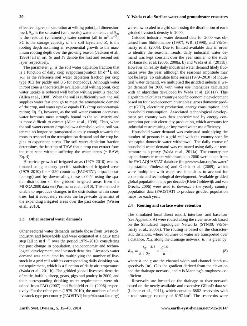
In Fig. 4 we compare simulated and reported trends ofgroundwater withdrawal per country over the period 1980–2005 in 5 yr intervals when the reported statistics are avail-able (the statistical data is not available before 1980). Thecomparison for 19 countries indicates that our approach isable to capture the decadal trends of groundwater with-drawal (R2>0.95,p value<0.001). The simulated trends ofgroundwater withdrawal match reasonably well with the ob-served trends not only for major groundwater users includ-ing the USA, China, and Mexico, but also for other coun-tries including Poland, Greece, Spain, and Slovakia. How-ever, the discrepancy between reported and observed trendstends to be larger for developed countries such as France, theUK, Austria, the Netherlands, and Finland. This suggests alimitation of our global application in which the partition-ing between surface water and groundwater withdrawal rep-resented by our approach needs further consideration or ad-justment for these countries.
4.3 Regional trends of surface water and groundwaterwithdrawal and consumption
In Figs. 5 and 6 we provide a regional overview of desali-nation water, surface water and groundwater withdrawal andconsumption over the period 1979–2010. Global water with-drawal and consumptive water use respectively increasedfrom ∼ 2000 and∼ 1000 km3 yr−1 in 1979 to∼ 3300 and∼ 1500 km3 yr−1 in 2010. This increase is primarily driven
Earth Syst. Dynam., 5, 15–40, 2014 www.earth-syst-dynam.net/5/15/2014/

Y. Wada et al.: Surface water and groundwater resources 25
0.001
0.01
0.1
1
10
100
1000
0.01
0.1
1
10
100
0.01
0.1
1
10
100
0.1
1
10
1
1
0.01
0.1
1
10
1
1
0.01
0.1
1
10
0.001 0.1 10 10000.01 1 100
0.01 0.1 1 10 100
0.01 0.1 1 10 100
0.1 1 10
0.001 0.1 10 10000.01 1 100
0.01 0.1 1 10 100
0.01 0.1 1 10 100
0.01 0.1 1 10 0.01 0.1 1 10
0.001 0.1 10 10000.01 1 100
0.01 0.1 1 10 100
0.01 0.1 1 10 100
Simulated value [km3 yr-1]
Rep
ort
ed v
alu
e [k
m3
yr-1]
Surface water useTotal water use Groundwater use
AA
BB
D
C
Fig. 3.Comparison of simulated total water withdrawals and water withdrawals per water source (surface water and groundwater) to reportedvalues [km3 yr−1] for the year 2005 over(a) the globe per country (N = 100), (b) Europe per country (N = 34), (c) the USA per state(N = 50), and(d) Mexico per state (N = 32) in log-log plots. Simulated water use at 0.5◦ was spatially aggregated to country and state.Simulated value indicates the mean of the simulation with the ERA-Interim and MERRA climate. Error bars show standard deviation (σ)
among the simulation with the ERA-Interim and MERRA climate. The dashed lines represent the 1:1 line. The reported water withdrawalper source was obtained from the FAO AQUASTAT database for the globe, from the Eurostat database (http://epp.eurostat.ec.europa.eu/portal/page/portal/environment/data/database) for Europe, from the US Geological Survey (Water Use in the United States;http://water.usgs.gov/watuse/) for the USA, and from the CONAGUA (Statistics on Water in Mexico;http://www.conagua.gob.mx/english07/publications/Statistics_Water_Mexico_2008.pdf) for Mexico.
by growth in the agricultural sector (mostly irrigation), ac-counting for as much as∼ 80 % of the total. Most of in-dustrial and domestic water that is withdrawn from surfacewater and groundwater returns to river systems (40–80 %).Surface water and groundwater withdrawal increased respec-tively from ∼ 1350 and∼ 650 km3 yr−1 in 1979 to∼ 2100and∼ 1200 km3 yr−1 in 2010. During the period 1979–1990,groundwater withdrawal increased by∼ 1 % per year, whilesurface water use rose by∼ 2 % per year. However, duringthe recent period 1990–2010, the rate of groundwater with-drawal increased to∼ 3 % per year, while that of surfacewater use decreased to∼ 1 %. This is likely due to the fact
that surface water has been extensively exploited in responseto the consistent increase of global water demands, whilethe construction of new (large) reservoirs has been decreas-ing since the 1990s (Chao et al., 2008). The results suggestthat the net increase in the demand has been mostly supple-mented by groundwater withdrawal. These trends can also beseen from the global change in consumptive water use dur-ing the period 1979–2010. Siebert et al. (2010), Kummu etal. (2010), and Wada et al. (2012a) also report an increas-ing dependency of consumptive water use on groundwaterresources in recent decades.
www.earth-syst-dynam.net/5/15/2014/ Earth Syst. Dynam., 5, 15–40, 2014
26 Y. Wada et al.: Surface water and groundwater resources
Fig. 4. Comparison of simulated and reported trends of groundwa-ter withdrawal per country over the period 1980–2005 (N = 19).The comparison is given in 5 yr interval according to the reportedvalues including missing values for some years. Countries are iden-tified with their ISO country codes:(a) the USA (USA) and China(CHN); (b) Mexico (MEX); (c) France (FRA), the UK (GBR),Poland (POL), Greece (GRC), and Spain (ESP);(d) Austria (AUT),Belgium (BEL), the Czech Republic (CZE), Finland (FIN), Is-rael (ISL), Luxemburg (LUX), Namibia (NAM), the Netherlands(NLD), Puerto Rico (PRI), Slovakia (SVK), and Sweden (SWE).Reported groundwater withdrawal was obtained from the FAOAQUASTAT database. Simulated value indicates the mean of thesimulation with the ERA-Interim and MERRA climate. Error barsshow standard deviation (σ) among the simulation with the ERA-Interim and MERRA climate. The dashed line represents the 1: 1slope.
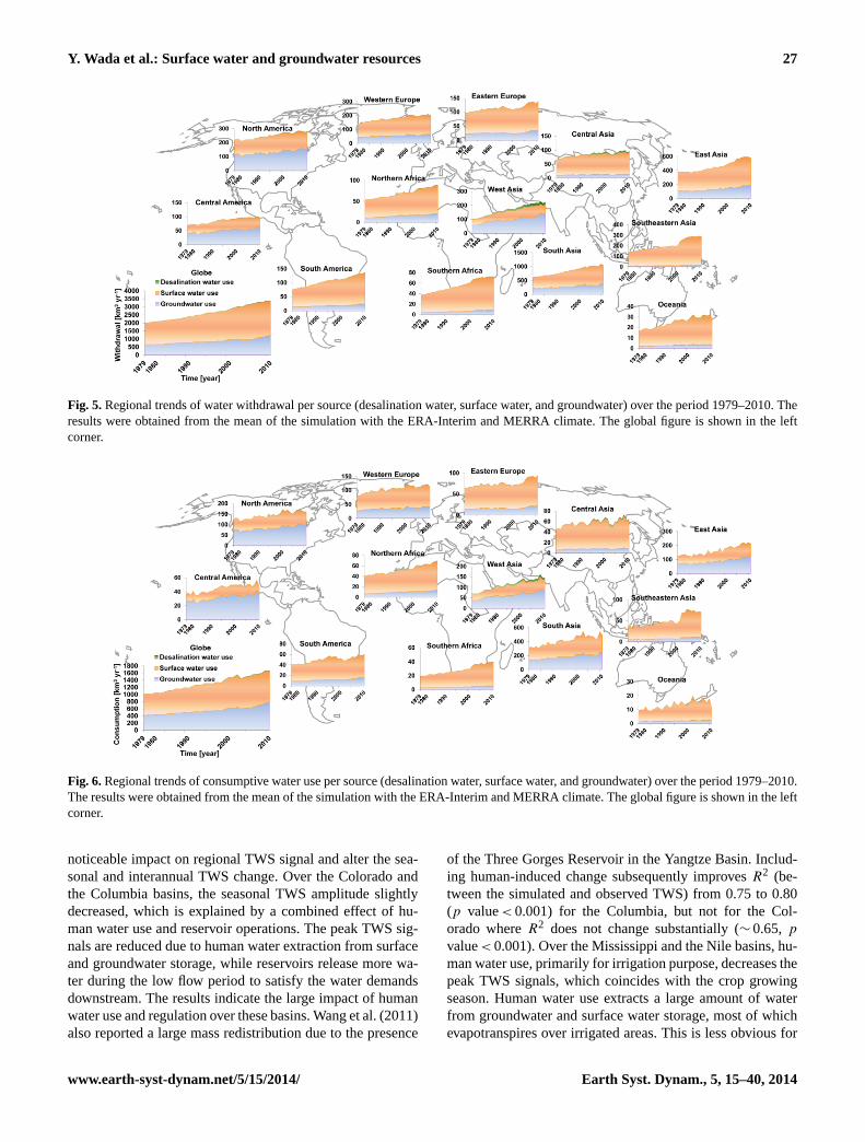
The regional trends of surface water and groundwaterwithdrawal and consumption exhibit very different trajec-tories over the period 1979–2010. Over Europe, ground-water withdrawal and consumption accounts for∼ 30 % ofthe total and has not increased substantially over the pastdecades. However, over North and Central America, ground-water withdrawal and consumption account for∼ 60 and∼ 70 % of the total, and have increased by more than 40 %over the last 30 yr. Over western Asia, groundwater with-drawal has tripled and accounts close to∼ 70 % of the total.Desalination water withdrawal accounts for 5 % of the to-tal and is rapidly increasing over the region. Over North andCentral America, and Asia, irrigation is the dominant wa-ter use sector and is predominantly relying on groundwaterresources (∼ 70 %). Over South and East Asia, surface wa-ter and groundwater withdrawal nearly doubled from∼ 600and∼ 360 km3 yr−1 in 1979 to∼ 1100 and∼ 600 km3 yr−1
in 2010, respectively. Total surface water and groundwaterwithdrawal over these regions accounts for more than halfof the global surface water and groundwater withdrawal re-spectively. Over the other regions, e.g., Southeast Asia andSouth America, surface water withdrawal exceeds∼ 80 %
of the total except in North Africa where groundwater with-drawal is substantial (>30 %). These trends are also visiblefrom the development of consumptive use of surface waterand groundwater (Fig. 6).
4.4 The impact of human-induced change on riverdischarge and terrestrial water storage change
Table 5 compares simulated river discharge under the pristineconditions (natural climate variability only) and under thehuman-induced change (human water use and reservoir oper-ations) with observed river discharge taken from the selectedGRDC stations (http://www.bafg.de/GRDC). For the com-parisons, we selected major basins of the world that cover awide range in climate and human impacts including reservoirregulation. Human-induced change is clearly observable forthe rivers crossing major irrigated areas of the world, giventhe number of existing reservoirs, including the Nile, the Or-ange, the Murray, the Mekong, the Ganges, the Indus, theYangtze, the Huang He, the Mississippi, the Columbia, andthe Volga. For the other river basins, the human impact is lessobvious, but still noticeable such as the Orinoco, the Parana,the Brahmaputra, the Danube, the Rhine, the Dnieper, and theElbe. For the Amazon, the Congo, the Niger, the Zambezi,the Mckenzie, and the Lena, the river discharge is hardly af-fected because of small reservoir capacity and lower humanwater use. For those river basins where human impacts arelarge, the performance of the simulated river discharge underthe pristine conditions tends to be lower compared to thatof the simulated river discharge under the human-inducedchange, except for the Huang He where our overall modelperformance is low. Overall, the correlation between the sim-ulated and the observed river discharge is high for most ofthe river basins, while the Nash–Sutcliffe model efficiencycoefficient is high for some river basins but low for severalbasins including the Nile, the Niger, and the Orange, wherethe number of observation records are limited.
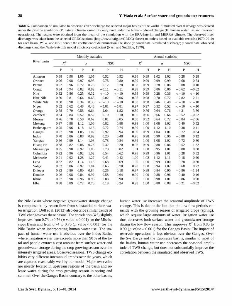
Figure 7 compares the simulated monthly terrestrial waterstorage (TWS) anomalies with those of the GRACE observa-tions (Liu et al., 2010) for a number of major river basins overthe period 2003–2010. The selection of the basins is rather ar-bitrary, but is based on the fact that they are heavily affectedby human activities, which enables to quantify the impact ofhuman water use and reservoir operations on terrestrial waterresources (e.g., surface water and groundwater). SimulatedTWS was calculated from the sum of simulated snow, surfacewater, soil water, and groundwater storage. The TWS anoma-lies were computed over the overlapping period of 2003–2010 with the GRACE data. Here, we compared two sim-ulation runs: one for pristine conditions (no human water useand no reservoirs) or natural climate variability only, and theother including human-induced change such as human wa-ter use (water withdrawal and consumptive water use) fromsurface water and groundwater storage, and reservoir oper-ations. The comparison shows that human activities have a
Earth Syst. Dynam., 5, 15–40, 2014 www.earth-syst-dynam.net/5/15/2014/
Y. Wada et al.: Surface water and groundwater resources 27
Fig. 5.Regional trends of water withdrawal per source (desalination water, surface water, and groundwater) over the period 1979–2010. Theresults were obtained from the mean of the simulation with the ERA-Interim and MERRA climate. The global figure is shown in the leftcorner.
Fig. 6.Regional trends of consumptive water use per source (desalination water, surface water, and groundwater) over the period 1979–2010.The results were obtained from the mean of the simulation with the ERA-Interim and MERRA climate. The global figure is shown in the leftcorner.
noticeable impact on regional TWS signal and alter the sea-sonal and interannual TWS change. Over the Colorado andthe Columbia basins, the seasonal TWS amplitude slightlydecreased, which is explained by a combined effect of hu-man water use and reservoir operations. The peak TWS sig-nals are reduced due to human water extraction from surfaceand groundwater storage, while reservoirs release more wa-ter during the low flow period to satisfy the water demandsdownstream. The results indicate the large impact of humanwater use and regulation over these basins. Wang et al. (2011)also reported a large mass redistribution due to the presence
of the Three Gorges Reservoir in the Yangtze Basin. Includ-ing human-induced change subsequently improvesR2 (be-tween the simulated and observed TWS) from 0.75 to 0.80(p value<0.001) for the Columbia, but not for the Col-orado whereR2 does not change substantially (∼ 0.65, pvalue<0.001). Over the Mississippi and the Nile basins, hu-man water use, primarily for irrigation purpose, decreases thepeak TWS signals, which coincides with the crop growingseason. Human water use extracts a large amount of waterfrom groundwater and surface water storage, most of whichevapotranspires over irrigated areas. This is less obvious for
www.earth-syst-dynam.net/5/15/2014/ Earth Syst. Dynam., 5, 15–40, 2014
28 Y. Wada et al.: Surface water and groundwater resources
Table 5.Comparison of simulated to observed river discharge for selected major basins of the world. Simulated river discharge was derivedunder the pristine conditions (P; natural climate variability only) and under the human-induced change (H; human water use and reservoiroperations). The results were obtained from the mean of the simulation with the ERA-Interim and MERRA climate. The observed riverdischarge was taken from the selected GRDC stations (http://www.bafg.de/GRDC) closest to outlets based on available records (1979-2010)for each basin.R2, α, and NSC denote the coefficient of determination, the slope (x coordinate: simulated discharge;y coordinate: observeddischarge), and the Nash–Sutcliffe model efficiency coefficient (Nash and Sutcliffe, 1970).
River basinMonthly statistics Annual statistics
R2 α NSC R2 α NSC
P H P H P H P H P H P H
Amazon 0.98 0.98 1.05 1.05 0.52 0.52 0.99 0.99 1.02 1.02 0.28 0.28Orinoco 0.96 0.98 0.97 0.98 0.78 0.80 0.99 0.99 0.99 0.99 0.68 0.74Parana 0.92 0.96 0.72 0.78 0.12 0.28 0.98 0.99 0.78 0.86 0.08 0.10Congo 0.94 0.94 0.82 0.82 −0.11 −0.11 0.99 0.99 0.86 0.86 −0.62 −0.62Nile 0.82 0.86 0.25 0.32 <−10 <−10 0.98 0.99 0.28 0.36 <−10 <−10Blue Nile 0.80 0.81 0.64 0.68 0.02 0.06 0.98 0.98 0.70 0.72−2.82 −2.21White Nile 0.88 0.90 0.34 0.38 <−10 <−10 0.98 0.98 0.46 0.48 <−10 <−10Niger 0.62 0.62 0.48 0.48 −5.81 −5.81 0.97 0.97 0.52 0.52 <−10 <−10Orange 0.68 0.70 0.58 0.64 −2.64 −1.82 0.80 0.86 0.64 0.76 −4.21 −3.86Zambezi 0.84 0.84 0.52 0.52 0.10 0.10 0.96 0.96 0.66 0.66−0.52 −0.52Murray 0.76 0.78 0.58 0.62 0.01 0.05 0.88 0.92 0.64 0.72−3.84 −2.86Mekong 0.97 0.98 1.12 1.06 0.82 0.88 0.99 1.00 1.08 1.02 0.40 0.52Brahmaputra 0.95 0.96 1.18 1.16 0.72 0.74 0.99 1.00 1.12 1.10 0.38 0.41Ganges 0.97 0.98 1.05 1.02 0.92 0.94 0.99 0.99 1.04 1.01 0.72 0.84Indus 0.78 0.86 0.88 0.92 0.20 0.48 0.96 0.98 0.90 0.96−0.88 0.12Yangtze 0.96 0.99 1.14 1.08 0.78 0.84 0.99 1.00 1.08 1.02 0.72 0.80Huang He 0.88 0.82 0.86 0.78 0.32 0.20 0.96 0.99 0.88 0.86−0.52 −1.82Mississippi 0.95 0.98 0.92 1.06 0.78 0.82 1.01 1.00 0.95 1.01 0.80 0.88Columbia 0.92 0.96 0.92 1.02 0.54 0.62 0.98 0.99 0.96 1.01 0.28 0.52Mckenzie 0.91 0.92 1.28 1.27 0.41 0.42 1.00 1.02 1.12 1.11 0.18 0.20Lena 0.82 0.82 1.14 1.15 0.68 0.69 1.00 1.00 0.99 1.00 0.78 0.80Volga 0.82 0.86 0.92 1.04 0.65 0.70 0.98 1.00 0.94 1.02 0.68 0.72Dnieper 0.82 0.80 0.80 0.84 0.25 0.18 0.97 0.99 0.84 0.90−0.86 −1.24Danube 0.96 0.98 0.84 0.92 0.58 0.64 0.99 1.00 0.88 0.96 0.40 0.46Rhine 0.97 0.98 0.96 0.98 0.88 0.90 1.00 1.00 0.98 1.01 0.86 0.90Elbe 0.88 0.89 0.72 0.76 0.18 0.24 0.98 1.00 0.80 0.88−0.21 −0.02
the Nile Basin where negative groundwater storage changeis compensated by return flow from substantial surface wa-ter irrigation. Döll et al. (2012) also describe similar trends ofTWS changes over these basins. The correlation (R2) slightlyimproves from 0.73 to 0.76 (p value<0.001) for the Missis-sippi Basin and from 0.74 to 0.76 (p value<0.001) for theNile Basin when incorporating human water use. The im-pact of human water use is obvious over the Indus Basin,where irrigation water use exceeds more than 90 % of the to-tal and people extract a vast amount from surface water andgroundwater storage during the crop growing season over theintensely irrigated areas. Observed seasonal TWS change ex-hibits very different interannual trends over the years, whichare captured reasonably well by our model. Major reservoirsare mostly located in upstream regions of the basin and re-lease water during the crop growing season in spring andsummer. Over the Ganges Basin, contrary to the other basins,
human water use increases the seasonal amplitude of TWSchange. This is due to the fact that the low flow periods co-incide with the growing season of irrigated crops (spring),which require large amounts of water. Irrigation water usethus decreases both surface water and groundwater storageduring the low flow season. This improvesR2 from 0.85 to0.90 (p value<0.001) for the Ganges Basin. The impact ofreservoir operations is less obvious over the Ganges. Overthe Syr Darya and the Euphrates basins, similar to most ofthe basins, human water use decreases the seasonal ampli-tude of TWS change, but does not substantially improve thecorrelation between the simulated and observed TWS.
Earth Syst. Dynam., 5, 15–40, 2014 www.earth-syst-dynam.net/5/15/2014/
Y. Wada et al.: Surface water and groundwater resources 29
-0.16 -0.12 -0.08 -0.04
0 0.04 0.08 0.12 0.16
-0.16 -0.12 -0.08 -0.04
0 0.04 0.08 0.12 0.16
-0.25 -0.2
-0.15 -0.1
-0.05 0
0.05 0.1
0.15 0.2
0.25
-0.15
-0.1
-0.05
0
0.05
0.1
0.15
-0.12
-0.08
-0.04
0
0.04
0.08
0.12
-0.1 -0.08 -0.06 -0.04 -0.02
0 0.02 0.04 0.06 0.08
0.1
-0.12
-0.08
-0.04
0
0.04
0.08
0.12
-0.1 -0.08 -0.06 -0.04 -0.02
0 0.02 0.04 0.06 0.08
0.1
2003 2004 2005 2006 2007 2008 2009 2010 2003 2004 2005 2006 2007 2008 2009 2010
TWS
An
om
aly
[m]
year
Colorado Columbia
Mississippi Nile
Indus Ganges
SyrDarya Euphrates
GRACE Pristine Humans
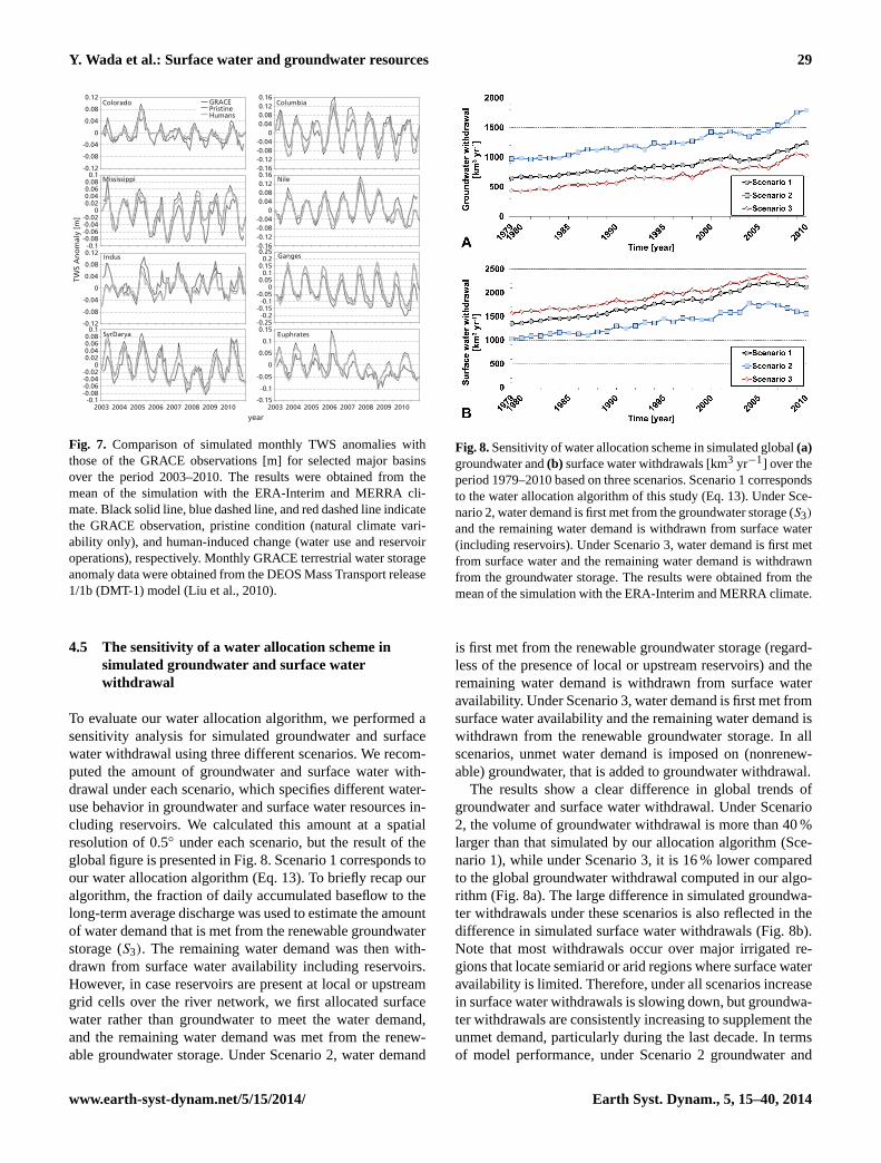
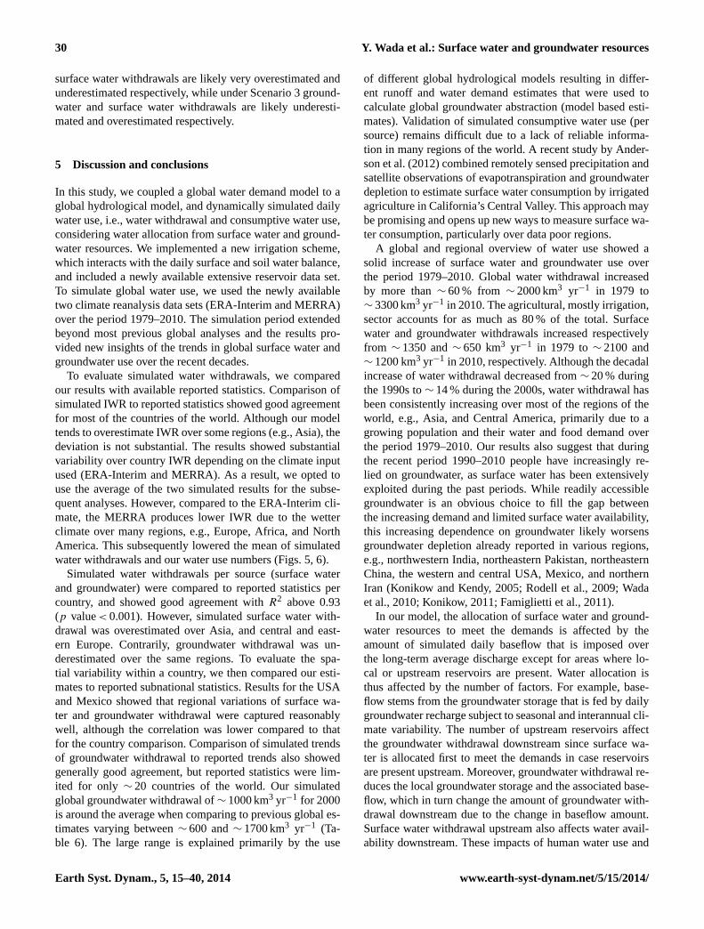
Fig. 7. Comparison of simulated monthly TWS anomalies withthose of the GRACE observations [m] for selected major basinsover the period 2003–2010. The results were obtained from themean of the simulation with the ERA-Interim and MERRA cli-mate. Black solid line, blue dashed line, and red dashed line indicatethe GRACE observation, pristine condition (natural climate vari-ability only), and human-induced change (water use and reservoiroperations), respectively. Monthly GRACE terrestrial water storageanomaly data were obtained from the DEOS Mass Transport release1/1b (DMT-1) model (Liu et al., 2010).
4.5 The sensitivity of a water allocation scheme insimulated groundwater and surface waterwithdrawal
To evaluate our water allocation algorithm, we performed asensitivity analysis for simulated groundwater and surfacewater withdrawal using three different scenarios. We recom-puted the amount of groundwater and surface water with-drawal under each scenario, which specifies different water-use behavior in groundwater and surface water resources in-cluding reservoirs. We calculated this amount at a spatialresolution of 0.5◦ under each scenario, but the result of theglobal figure is presented in Fig. 8. Scenario 1 corresponds toour water allocation algorithm (Eq. 13). To briefly recap ouralgorithm, the fraction of daily accumulated baseflow to thelong-term average discharge was used to estimate the amountof water demand that is met from the renewable groundwaterstorage (S3). The remaining water demand was then with-drawn from surface water availability including reservoirs.However, in case reservoirs are present at local or upstreamgrid cells over the river network, we first allocated surfacewater rather than groundwater to meet the water demand,and the remaining water demand was met from the renew-able groundwater storage. Under Scenario 2, water demand
Fig. 8.Sensitivity of water allocation scheme in simulated global(a)groundwater and(b) surface water withdrawals [km3 yr−1] over theperiod 1979–2010 based on three scenarios. Scenario 1 correspondsto the water allocation algorithm of this study (Eq. 13). Under Sce-nario 2, water demand is first met from the groundwater storage (S3)
and the remaining water demand is withdrawn from surface water(including reservoirs). Under Scenario 3, water demand is first metfrom surface water and the remaining water demand is withdrawnfrom the groundwater storage. The results were obtained from themean of the simulation with the ERA-Interim and MERRA climate.
is first met from the renewable groundwater storage (regard-less of the presence of local or upstream reservoirs) and theremaining water demand is withdrawn from surface wateravailability. Under Scenario 3, water demand is first met fromsurface water availability and the remaining water demand iswithdrawn from the renewable groundwater storage. In allscenarios, unmet water demand is imposed on (nonrenew-able) groundwater, that is added to groundwater withdrawal.
The results show a clear difference in global trends ofgroundwater and surface water withdrawal. Under Scenario2, the volume of groundwater withdrawal is more than 40 %larger than that simulated by our allocation algorithm (Sce-nario 1), while under Scenario 3, it is 16 % lower comparedto the global groundwater withdrawal computed in our algo-rithm (Fig. 8a). The large difference in simulated groundwa-ter withdrawals under these scenarios is also reflected in thedifference in simulated surface water withdrawals (Fig. 8b).Note that most withdrawals occur over major irrigated re-gions that locate semiarid or arid regions where surface wateravailability is limited. Therefore, under all scenarios increasein surface water withdrawals is slowing down, but groundwa-ter withdrawals are consistently increasing to supplement theunmet demand, particularly during the last decade. In termsof model performance, under Scenario 2 groundwater and
www.earth-syst-dynam.net/5/15/2014/ Earth Syst. Dynam., 5, 15–40, 2014
30 Y. Wada et al.: Surface water and groundwater resources
surface water withdrawals are likely very overestimated andunderestimated respectively, while under Scenario 3 ground-water and surface water withdrawals are likely underesti-mated and overestimated respectively.
5 Discussion and conclusions
In this study, we coupled a global water demand model to aglobal hydrological model, and dynamically simulated dailywater use, i.e., water withdrawal and consumptive water use,considering water allocation from surface water and ground-water resources. We implemented a new irrigation scheme,which interacts with the daily surface and soil water balance,and included a newly available extensive reservoir data set.To simulate global water use, we used the newly availabletwo climate reanalysis data sets (ERA-Interim and MERRA)over the period 1979–2010. The simulation period extendedbeyond most previous global analyses and the results pro-vided new insights of the trends in global surface water andgroundwater use over the recent decades.
To evaluate simulated water withdrawals, we comparedour results with available reported statistics. Comparison ofsimulated IWR to reported statistics showed good agreementfor most of the countries of the world. Although our modeltends to overestimate IWR over some regions (e.g., Asia), thedeviation is not substantial. The results showed substantialvariability over country IWR depending on the climate inputused (ERA-Interim and MERRA). As a result, we opted touse the average of the two simulated results for the subse-quent analyses. However, compared to the ERA-Interim cli-mate, the MERRA produces lower IWR due to the wetterclimate over many regions, e.g., Europe, Africa, and NorthAmerica. This subsequently lowered the mean of simulatedwater withdrawals and our water use numbers (Figs. 5, 6).
Simulated water withdrawals per source (surface waterand groundwater) were compared to reported statistics percountry, and showed good agreement withR2 above 0.93(p value<0.001). However, simulated surface water with-drawal was overestimated over Asia, and central and east-ern Europe. Contrarily, groundwater withdrawal was un-derestimated over the same regions. To evaluate the spa-tial variability within a country, we then compared our esti-mates to reported subnational statistics. Results for the USAand Mexico showed that regional variations of surface wa-ter and groundwater withdrawal were captured reasonablywell, although the correlation was lower compared to thatfor the country comparison. Comparison of simulated trendsof groundwater withdrawal to reported trends also showedgenerally good agreement, but reported statistics were lim-ited for only ∼ 20 countries of the world. Our simulatedglobal groundwater withdrawal of∼ 1000 km3 yr−1 for 2000is around the average when comparing to previous global es-timates varying between∼ 600 and∼ 1700 km3 yr−1 (Ta-ble 6). The large range is explained primarily by the use
of different global hydrological models resulting in differ-ent runoff and water demand estimates that were used tocalculate global groundwater abstraction (model based esti-mates). Validation of simulated consumptive water use (persource) remains difficult due to a lack of reliable informa-tion in many regions of the world. A recent study by Ander-son et al. (2012) combined remotely sensed precipitation andsatellite observations of evapotranspiration and groundwaterdepletion to estimate surface water consumption by irrigatedagriculture in California’s Central Valley. This approach maybe promising and opens up new ways to measure surface wa-ter consumption, particularly over data poor regions.
A global and regional overview of water use showed asolid increase of surface water and groundwater use overthe period 1979–2010. Global water withdrawal increasedby more than∼ 60 % from ∼ 2000 km3 yr−1 in 1979 to∼ 3300 km3 yr−1 in 2010. The agricultural, mostly irrigation,sector accounts for as much as 80 % of the total. Surfacewater and groundwater withdrawals increased respectivelyfrom ∼ 1350 and∼ 650 km3 yr−1 in 1979 to∼ 2100 and∼ 1200 km3 yr−1 in 2010, respectively. Although the decadalincrease of water withdrawal decreased from∼ 20 % duringthe 1990s to∼ 14 % during the 2000s, water withdrawal hasbeen consistently increasing over most of the regions of theworld, e.g., Asia, and Central America, primarily due to agrowing population and their water and food demand overthe period 1979–2010. Our results also suggest that duringthe recent period 1990–2010 people have increasingly re-lied on groundwater, as surface water has been extensivelyexploited during the past periods. While readily accessiblegroundwater is an obvious choice to fill the gap betweenthe increasing demand and limited surface water availability,this increasing dependence on groundwater likely worsensgroundwater depletion already reported in various regions,e.g., northwestern India, northeastern Pakistan, northeasternChina, the western and central USA, Mexico, and northernIran (Konikow and Kendy, 2005; Rodell et al., 2009; Wadaet al., 2010; Konikow, 2011; Famiglietti et al., 2011).
In our model, the allocation of surface water and ground-water resources to meet the demands is affected by theamount of simulated daily baseflow that is imposed overthe long-term average discharge except for areas where lo-cal or upstream reservoirs are present. Water allocation isthus affected by the number of factors. For example, base-flow stems from the groundwater storage that is fed by dailygroundwater recharge subject to seasonal and interannual cli-mate variability. The number of upstream reservoirs affectthe groundwater withdrawal downstream since surface wa-ter is allocated first to meet the demands in case reservoirsare present upstream. Moreover, groundwater withdrawal re-duces the local groundwater storage and the associated base-flow, which in turn change the amount of groundwater with-drawal downstream due to the change in baseflow amount.Surface water withdrawal upstream also affects water avail-ability downstream. These impacts of human water use and
Earth Syst. Dynam., 5, 15–40, 2014 www.earth-syst-dynam.net/5/15/2014/

Y. Wada et al.: Surface water and groundwater resources 31
Table 6.Global estimates of groundwater abstraction.
Total/NonrenewableGroundwater Withdrawal/ Runoff/
[km3 yr−1] abstraction1 Year Consumption Recharge Sources
Data based estimates
Postel (1999) –/∼ 200 Contemporary – – Literature and country statisticsIGRAC-GGIS ∼ 750/– 2000 – – Literature and country statisticsShah et al. (2000) 750–800/– Contemporary – – FAO AQUASTAT, Llamas et al. (1992)Zekster and Everett (2004) 600–700/– Contemporary – – Country statistics
Model based estimates
Vörösmarty et al. (2005) –/389Irr.−830Tot. Avg. 1995–2000 3557Total/1206Irr. 39 294/– Simulated by WBM (0.5◦)
Rost et al. (2008) –/730 Avg. 1971–2000 2534–2566/1353–1375 36 921/– Simulated by LPJmL (0.5◦)Döll (2009) 1100/– 2000 4020/1300 38 800/– IGRAC-GGIS and WaterGAP (0.5◦)Wisser et al. (2010) 1708/1199 Contemporary 2997/– 37 401/– Simulated by WBMplus (0.5◦)Hanasaki et al. (2010) –/703 Avg. 1985–1999 –/1690 41 820/– Simulated by H08 (1.0◦)Siebert et al. (2010) 545/– 2000 –/1277 39 549/12 600 15 038 national/subnational statistics (irrigation)Wada et al. (2010) 734 (± 82)/283 (± 40) 2000 –/– 36 200/15 200 IGRAC-GGIS and PCR-GLOBWB (0.5◦)Pokhrel et al. (2012a) –/455 (± 42) 2000 2462 (± 130)/1021 (± 55) –/– Simulated by MATSIRO (1.0◦)Döll et al. (2012) ∼ 1500/– Avg. 1998–2002 4300/1400 –/– IGRAC-GGIS and WaterGAP (0.5◦)
1 Some model based studies also include the estimate of nonlocal water abstraction (e.g., water supplied from cross-basin water diversions).
reservoirs are accumulated along the river network and be-come substantial over heavily affected basins (e.g., the In-dus, the Colorado, and the Mississippi). Note that the tempo-ral increase in simulated groundwater withdrawal is drivenstrongly by the increase in total water demand and the vari-ability in surface water availability including reservoirs overthe period 1979–2010.
The analysis of simulated TWS anomalies revealed thathuman water use and associated reservoir operation alterthe seasonal and interannual variability of TWS change.The alteration is particularly large over heavily regulatedbasins, e.g., the Colorado and Columbia basins, and overbasins with major irrigated regions, e.g., the Mississippi, In-dus, and Ganges basins. Including human water use gener-ally improves the correlation of simulated TWS anomalieswith those of the GRACE observations over basins (e.g., theColumbia, the Mississippi, and the Ganges). Note that themodel performance is low over some of the simulation pe-riod for some basins, e.g., 2003 for the Indus, the Syr Darya,and the Euphrates, and 2006 for the Indus and the Euphrates.Nevertheless, the model reproduces TWS adequately formost of the basins.
To account for the climate uncertainty, we used two inde-pendent climate data sets: ERA-Interim and MERRA. How-ever, model uncertainty can be large since model outputs canvary substantially among different global hydrological mod-els (GHMs) with different model structure (Gosling et al.,2010, 2011; Haddeland et al., 2011). Nevertheless, our sim-ulated water use shows good agreement with reported statis-tics for most countries of the world. Moreover, our simulatedTWS anomalies also show reasonable agreement with ob-served TWS data, but the comparison is limited to the se-lected major basins of the world where human impacts aresubstantial.
Our integrated modeling framework is capable of simulat-ing human water use more realistically by including newlydeveloped approaches. Our irrigation scheme is based on thesurface and soil moisture deficit for paddy and nonpaddyfields respectively, and considers the feedback between dailyirrigation and associated changes in surface and soil moisturecondition. This, in turn, influences the amount of daily evap-otranspiration on the same day and the soil moisture in fol-lowing days over irrigated areas. Compared to earlier work(Wada et al., 2012a, b), the calculation of return flow fromirrigation is more realistic considering the soil water balanceand associated percolation losses underlying irrigated areas,which substantially contributes to groundwater recharge. In-cluding the fine temporal dynamics of irrigation water re-quirement is critical as it concerns the daily water withdrawalto satisfy the demand, which affects the amount of wateravailable downstream through river network. The model alsocalculates the other daily sectoral water demands includinglivestock, industry, and households, and considers the sea-sonal pattern of the demands (except the industry), whilemost of other GHMs calculate these demands on an annualbasis. Our improved approach also includes a water alloca-tion scheme that distinguishes surface water and groundwa-ter withdrawals dynamically at a daily temporal resolution.Water is withdrawn and consumed from groundwater andavailable river discharge including the effect of reservoir op-erations that are parameterized using a newly available ex-tensive global reservoir data set. Groundwater withdrawalalso affects the amount of baseflow that is calculated withthe available groundwater storage with the reservoir coeffi-cient (see Appendix A), which in turn changes the amount ofgroundwater withdrawal downstream. These series of anthro-pogenic impacts on surface water and groundwater resourcesare reflected on the terrestrial water storage change, which
www.earth-syst-dynam.net/5/15/2014/ Earth Syst. Dynam., 5, 15–40, 2014
32 Y. Wada et al.: Surface water and groundwater resources
was well captured in our analysis using the GRACE observa-tion. Thus, our new modeling framework enables one to com-prehensively assess human-induced change in global watersystems and to track those changes over time. The sensitivityanalysis to assess our water allocation scheme showed thatour scheme is preferred for the simulation of water use be-havior compared to the other scenarios that prioritize eithergroundwater or surface water withdrawal first to meet the wa-ter demand.
However, there are certain limitations and major assump-tions, that should be sufficiently addressed. First, alloca-tion of surface water and groundwater to satisfy the sec-toral water demands is currently simulated in a simplisticway using the faction of daily accumulated baseflow to thelong-term average discharge and the number of available lo-cal and upstream reservoirs. Simulated (accumulated) base-flow is used to infer the readily extractable groundwater re-serves. This assumption may be realistic in semiarid andarid regions where people largely rely on groundwater re-sources to satisfy the demands (e.g., northern India, Pak-istan, northern China, Iran, and Mexico). However, thereare likely discrepancies over regions where people predom-inantly rely on surface water resources despite the presenceof the readily accessible groundwater reserves over shallowgroundwater tables (e.g., humid regions). In addition, al-though the influence may not be large at the global scale,groundwater pumping is regulated in many developed coun-tries (e.g., Japan, the Netherlands, Germany, and France),while water use management including pumping regulationis not accounted for in our model. Moreover, a realistic rep-resentation of the groundwater table considering lateral flow(Fan et al., 2013) is not incorporated, but it may substantiallyaffect the simulation of groundwater storage and associatedbaseflow. Such process is important over aquifers with hightransmissivity. Second, long-distance and cross-basin waterdiversions (e.g., aqueducts) provide additional surface wa-ter availability, which may substantially contribute to supplyirrigation water requirement over regions such as the Indo-Gangetic plains, California’s Central Valley, and the Col-orado River, where extensive diversion works are present.Some information is available, e.g., the Periyar Project (max-imum capacity: 40 m3 s−1) and the Kurnool Cudappah Canal(maximum capacity: 85 m3 s−1) in India, and the Irtysh–Karaganda Canal (maximum capacity: 75 m3 s−1 in Cen-tral Asia (World Bank; http://www.worldbank.org/; UNDP;http://www.undp.org). However, artificial diversion networksand the actual amount of water transferred are difficult tobe parameterized, and are not represented in our modelingframework due to limited data available worldwide. Third,we assumed that return flow from the industrial and domesticsectors to the river system occurs on the same day as wateris withdrawn, but retention likely occurs due to waste wa-ter treatment, particularly in developed countries. Finally, al-though we used the recycling ratios developed on the basisof country GDP, the amount of water recycling to calculate
consumptive water use is difficult to verify due to the lack of(sub-)national statistics over many regions of the world.
This study builds upon previous modeling efforts and con-tributes to improve a current modeling framework that quan-tifies the impact of anthropogenic impacts on global waterresources. Despite its limitations, our modeling frameworkadvances an important step beyond earlier work by attempt-ing to account more realistically for the behavior of humanwater use and associated impacts on the terrestrial water sys-tem. It can be also used to assess future increase in water useper source due to population growth and economic develop-ment that will pose a serious threat to regions currently undersubstantial water scarcity and groundwater depletion, and toidentify regions of looming water scarcity under future cli-mate or under envisaged socioeconomic developments.
Appendix A
Here we present the essential and recently updated featuresof the model (Van Beek et al., 2011). The newly developedparts of the model are described in the main manuscript. Themodel is a grid-based model of global terrestrial hydrology(excluding Antarctica), which is essentially a leaky-buckettype of model, but a certain consideration is given represent-ing the groundwater reservoir.
A1 Snow accumulation and melt
Over each grid cell, precipitation falls in the form of rainor snow. Any precipitation that falls on the soil surface canbe intercepted by vegetation and in part or in whole evapo-rated. Snow accumulation and melt are temperature drivenand modeled according to the snow module of the HBVmodel (Bergström, 1995). To represent the rain–snow tran-sition over subgrid elevation dependent gradients of temper-ature, 10 elevation zones were made on each grid cell basedon the HYDRO1k, and scaled the 0.5◦ grid temperate fieldswith a lapse rate of 0.65◦C per 100 m. Over the 10 eleva-tion zones, precipitation accumulates as snow if the tem-perature,T , is below the melt temperature (0◦C), Tm. Thesnowmelt [m], SCmelt, is then modeled using a degree dayfactor [m◦C−1 day−1], fd:
SCmelt = fd (T − Tm) , (A1)
Above the melt temperature, precipitation and melt water arestored as liquid water in the available pore space in the snowcover. Melt water in the snow cover can refreeze dependingon the water holding capacity of the snow (10 % of snowwater equivalent) or evaporate. Snow is accumulated whenthe temperature is sufficiently low, otherwise it will melt andbe added to the net liquid precipitation (Pnet) that reachesthe soil as rain or throughfall. Excess water from snowmeltand rainfall forms direct runoff or infiltrates into the first soillayer (S1), which can further infiltrate into the second soil
Earth Syst. Dynam., 5, 15–40, 2014 www.earth-syst-dynam.net/5/15/2014/
Y. Wada et al.: Surface water and groundwater resources 33
layer (S2) and percolates into the third groundwater reservoir(S3).
A2 Infiltration and direct runoff
Liquid water passed on from the snow cover to the soil sur-face will infiltrate if sufficient water storage is available, elseit will drain over the surface as direct runoff. The partitioninginto infiltration and direct runoff is dependent on the degreeof saturation and the distribution of available water storagein the soil (Todini, 1996).
x = 1−
(Wmax−W
Wmax−Wmin
) bb+1
, (A2)
whereWmax is the total water storage capacity (SCS1 + SCS2)
[m]. Wmin is the minimum water storage capacity [m] ac-cording to the improved Arno scheme (IA) (Hagemann andGates, 2003).W is the actual water storage (SS1 +SS2) [m].To determine the water storages, the sum of the two uppersoil layers and the average of each grid cell (0.5◦) are consid-ered. The parameter,b, is the dimensionless shape factor thatdefines the distribution of soil water storage within the cell.b is calculated based on the distribution of maximum root-ing depths, which is derived from the 1 km by 1 km GlobalLand Cover Characteristics database version 2.0 (GLCC 2.0;http://edc2.usgs.gov/glcc/globe_int.php) and the land surfaceparameter data set (LSP2; Hagemann, 2002). To avoid anoverestimation due to the zero (minimum) water storage ca-pacity that always yields direct runoff when water falls ontothe soil, the minimum water storage capacity was adjustedaccording to the IA (Hagemann and Gates, 2003). This al-lows a reasonable response time over which a minimum stor-age needs to be filled before any direct runoff will occur.
Direct runoff,Qdirect [m d−1], can occur for each time step[day] whenPnet [m d−1] falls over the surface and the sum ofthe actual water storage and the liquid precipitation exceedsWmin. Moreover, any liquid precipitation is converted intodirect runoff once pervious area is completely saturated.
Qdirect =0 (Pn+W ≤Wmin)
Pn−1W +1Wmax
((1W1Wmax
) 1b+1
−Pn
(b+1)1Wmax
)b+1
(Wmin < Pn+W ≤Wmax)
Pn−1W (Pn+W >Wmax)
(A3)
where1Wmax is the range between the maximum and theminimum water storage (Wmax–Wmin) [m], and1W is therange between the maximum and the actual water storage(Wmax–W ) [m].
qi,Pnet→S1 = Pnet−Qdirect , (A4)
whereqi is the infiltration [m d−1] from Pnet to S1 calcu-lated from the difference betweenPnet, andQdirect, aug-mented with any initial water storage to replenish the stor-age toWmin. When the infiltration rate exceeds the saturatedhydraulic conductivity (ksat) of S1 [m d−1], the infiltrationexcess is passed on to the direct runoff.
A3 Soil evaporation and transpiration
Soil moisture is liable to soil evaporation when the surface isbare and to transpiration when vegetated. Actual evapotran-spiration is partitioned into soil evaporation and plant tran-spiration. Soil evaporation can occur from the top soil layer(S1) over which the evaporation rate is limited by the satu-rated conductivity,ksat, in the saturated area,Asat (x), and bythe unsaturated conductivity,k(θE), in the unsaturated area,Auns (1-x). The evaporation amount is considered separatelyfor soil,Esoil [m d−1], and melt water stored in snow cover,Esnow [m d−1].
Esoil,S1 = Asat× min(ksat,S1,Epot,S1 −Esnow)
+Auns× min(k(θE)S1,Epot,S1 −Esnow) (A5)
Potential soil evaporation rate,Epot,S1[m d−1], is calculatedfrom the difference between the reference (potential) evapo-transpiration and the actual evaporation from the interceptionstorage,Eint [m d−1]. This amount is multiplied with the cropfactor of the bare soil (∼ 0.2),kc,soil [dimensionless] over thenonvegetated surface (1-Cf).
Epot,S1 = (ET0 −Eint)× kc,soil × (1−Cf) (A6)
Esnow= min(SCmelt,Epot,S1) (A7)
Eint = min(Sint, (kc,vegET0 − kc,soilET0)), (A8)
whereSint is the interception storage [m] andkc,vegis the cropfactor of each vegetation cover [dimensionless]. The modelconsiders four vegetation covers: short (grassland) and tall(forest) natural vegetation, paddy crops, and nonpaddy crops.Vegetation cover fraction,Cf [dimensionless], is parameter-ized using the GLCC 2.0 and the global ecosystem classifi-cation of Olson (1994a, b), LSP2, and the MIRCA2000 dataset.
Vegetation extracts water from the two soil layers (S1 andS2) by transpiration except when the soil is saturated, whichprevents root water uptake due to the lack of aeration. There-fore, transpiration occurs only over the unsaturated area,Auns(1−x).
Tc = Tc,pot×Auns× ftrans (A9)
Tc,pot= (kc,vegET0 −Epot,S1 −Eint)×Cf (A10)
The influence of available soil moisture on root water up-take (∼ actual transpiration) is quantified by means of thefraction,ftrans [dimensionless], that is based on the effectivedegree of saturation (θE,ftrans), the effective degree of satu-ration at which the potential transpiration is halved (θE50),and the corresponding coefficient of the soil water retentioncurve (β). The actual transpiration rate,Tc [m d−1], is thencalculated by multiplying the potential transpiration,Tc,pot[m d−1], and the fraction (ftrans).
ftrans=1
1+(θE,ftrans
/θE50
)−3β50(A11) (A11)
www.earth-syst-dynam.net/5/15/2014/ Earth Syst. Dynam., 5, 15–40, 2014
34 Y. Wada et al.: Surface water and groundwater resources
θE,ftrans =
Wmax+ b (1Wmax)
[1−
b+1b
(1W1Wmax
) 1b+1
]Wmax+ b (1Wmax)
[1−
(1W1Wmax
) 1b+1
] (A12)
The actualTc is partitioned over the two soil layers (S1 andS2) according to the root fraction distribution,rf [dimension-less], in the two soil layers.
Tc,S1 =rf,S1SS1
rf,S1SS1 + rf,S2SS2× Tc (A13)
Tc,S2 =rf,S2SS2
rf,S1SS1 + rf,S2SS2× Tc (A14)
When the available soil moisture is limited to accommodatethe overall fluxes, the overall fluxes are reduced proportion-ally to the amount of their original fluxes.
A4 Vertical water fluxes in soil and groundwater stores
Water moves throughS1 andS2 and the third groundwaterlayer (S3). Vertical water fluxes [m d−1] betweenS1 andS2are driven by the effective degree of saturation of both layers,θE,S1 = SS1/SCS1 andθE,S2 = SS2/SCS2 or θE,S1 = θS1/θsat,S1and θE,S2 = θS2/θsat,S2. θ is the effective moisture contentdefined as the fraction of water storage to soil depth (θS1 =SS1/ZS1 andθS2 = SS2/ZS2). Percolation,qp,S1→S2 [m d−1],from S1 to S2 is governed by the rate of unsaturated hy-draulic conductivity ofS1, k(θE)S1 [m d−1] if sufficient soilmoisture is available. However, whenθE,S1< θE,S2, upwardcapillary flux (capillary rise) can occur at the rate of unsatu-rated hydraulic conductivity of the second soil layer,k(θE)S2[m d−1], but is limited to the portion of soil moisture deficitof the overlaying layer (1-θE,S1).
Cr,S2→S1 =(1− θE,S1
)× k (θE)S2 (A15)
Otherwise, the capillary flux is set to zero (θE,S1 ≥ θE,S2).The unsaturated hydraulic conductivity of each soil layer isdependent on the effective degree of saturation (Clapp andHornberger, 1978) and is calculated as
k(θE)= ksat× θ2β+3E , (A16)
whereβ is a dimensionless empirical exponent that varies onaverage between∼ 4 and∼ 11 over the range from sand toclay soil. It is based on a soil water retention curve parame-ter developed by Clapp and Hornberger (1978), who describethe relationship between the effective degree of saturationand the soil matric suction,ψ [m], as
ψ = ψsat× θ−βE , (A17)
whereψsat is the soil matric suction at saturation [m].Vertical water exchange, i.e., deep percolation,qp,S2→S3
[m d−1], and capillary rise,Cr,S3→S2 [m d−1], betweenS2and S3 is calculated in a similar way, except that the rate
is given in the geometric mean of the unsaturated hydraulicconductivity ofS2 and the saturated hydraulic conductivityof S3:
Cr,S3→S2 =√k (θE)S2 × ksat,S3 × (1− θE,S2)
×0.5f5m(θE,S2 < θE FC,S2,SS3 > 0). (A18)
Capillary rise only occurs given the proximity of the water ta-ble and the resulting moisture content ofS2 cannot rise abovefield capacity,θE FC,S2 (with ψfc = 1.0 m).SS3 is the waterstorage inS3 [m]. f5m is the fraction of the grid cell witha groundwater depth within 5 m. Capillary rise is at maxi-mum when the groundwater level is at the surface and it be-comes zero when the groundwater level is below 5 m fromthe surface. The factor 0.5 is an estimate of the average cap-illary flux that occurs over the area fraction (f5m) with agroundwater table within 5 m depth. The fraction (f5m) isdetermined from the groundwater depth distribution. First all1 km× 1 km grid cells are determined within the 0.5◦
× 0.5◦
grid that belongs to the perennial drainage network. Us-ing thePerennial Inland Water Areas of the World(Vmap0;FAO, 1997), the average drainage density,D [m−1] is esti-mated (i.e., total length of perennial water courses dividedby catchment area). For each of these grid cells, the up-stream drainage area of the catchment is determined usingthe HYDRO1k. Next, taking the actual water levels (simu-lated by the model) of the perennial stream cells as a ref-erence, the groundwater height [m],H = SS3/fd (with fddrainable porosity or specific yield) is added to arrive at alocal groundwater level and groundwater depth. From thegroundwater depth distribution for each catchment, the areawith a groundwater depth smaller than 5 m is determined.Adding these areas for all catchments and dividing by thetotal 0.5◦ × 0.5◦ grid cell area gives the estimates of the frac-tion (f5m).
A5 Interflow or subsurface storm flow
In mountainous areas soils develop in regolith (unconsoli-dated solid material) covering the bedrock. The steep gra-dient of high (soil) to low (bedrock) hydraulic conductivityresults in the occurrence of perched groundwater bodies dur-ing wet periods, which will cause a fast downslope flux ofwater through the soils down to the water courses. The modelcalculates this lateral drainage fromS2 over the height of thesaturated wedge that may form over the contact withS3. Thisoccurs when percolation fromS1 is high and percolation toS3 is low, which results in the high gradient that drives lateralflow along the slope. This lateral drainage, known as inter-flow or subsurface storm flow, is modeled according to Sloanand Moore (1984):
Qint,t (Ls)=
[1−
1t
TCL
]Qint,t−1(Ls)+
1t
TCLLs (A19)[
(qp,S1→S2,t +Cr,S3→S2,t )− (qp,S2→S3,t +Cr,S2→S1,t )],
Earth Syst. Dynam., 5, 15–40, 2014 www.earth-syst-dynam.net/5/15/2014/
Y. Wada et al.: Surface water and groundwater resources 35
TCL =Ls× θav,S2
2× ksat,S2 × tan(αs), (A20)
whereLs is the average slope length [m] and1t is the timestep [day]. TCL is the centroid-lag time or the characteristicresponse time [days].θav is the available pore space basedon the difference between the saturated (volumetric) mois-ture content (θsat) and the (volumetric) soil moisture con-tent at field capacity (θFC) or θav,S2 = θsat,S2 − θFC,S2 [all inm3 m−3]. tan(αs) is the gradient equal to the tangent of theslope angle [dimensionless]. The average slope is determinedfrom the average of calculated slopes from the 1 km× 1 kmHYDRO1k within the 0.5◦ × 0.5◦ grid cell, excluding thelowest 10 % of the elevations, which are assumed to be partof the floodplain.
Interflow,Qint [m3 d−1], is modeled along the slope (Ls)
as a function of the lateral drainage (interflow) over the previ-ous time step and the present recharge adding to or drawingfrom saturated wedge, taking into account the centroid-lagtime. It is assumed that the saturated wedge responds to therecharge without delay and that it always will be drainingwith the available pore space. The recharge here is the netpercolation, being the total of the gains to the second storedue to percolation from the top soil layer and the capillaryrise from the underlying groundwater layer as well as that ofthe losses due to percolation to the groundwater layer and thecapillary rise to the top soil layer. Interflow is assumed to oc-cur over areas with steep slopes and bedrock (i.e., mountain-ous areas). We calculated within the 0.5◦
× 0.5◦ grid cell thefraction of soils with a soil depth smaller than 1.5 m (max-imum soil depth in the model) and used this as a proxy forthe areas with the occurrence of interflow.Qint is calculatedin terms of area per time step [m2 d−1], but rather expressedas height per time step [m d−1] by dividing both terms ofEq. (A19) byLs [m].
A6 Baseflow
S3 represents the deeper part of the soil that is exempt fromany direct influence of vegetation and constitutes a ground-water reservoir fed by active recharge fromS2. The activegroundwater recharge consists of the net percolation that iscalculated from the difference between the deep percolation(qp,S2→S3) and the capillary rise (Cr,S3→S2). Drainage fromthe groundwater reservoir contributes as baseflow to the to-tal river discharge. Groundwater discharge (baseflow) con-tributes an important part to streamflow in many parts of theworld, particularly during low flow conditions. In the model,the groundwater storage and discharge are modeled by a firstorder linear reservoir approach. Baseflow,Qbase [m d−1],is modeled by multiplying groundwater store,SS3 [m], andthe reservoir or recession coefficient parameterized based ondrainage theory (liner reservoir) developed by Kraaijenhoffvan de Leur (1958),J [days].J is the spatial variable with alarge regional variability, representing the average residence
time of water in the groundwater store.
SS3,t = SS3,t−1 −Qbase,t−1 + (qp,S2→S3,t −Cr.S3→S2,t ) (A21)
Qbase,t = SS3,t × J (A22)
J =π2(ksat,S3 ×Dc)
4× fd ×B2c
, (A23)
whereksat,S3 is the saturated hydraulic conductivity of theaquifer (S3), fd is the drainable porosity,Dc is the aquiferdepth [m] andBc is the drainage length [m]. The parame-ter Bc is obtained from the drainage density analysis. Thesaturated hydraulic conductivity and drainable porosity havebeen related to a simplified version (7 classes) of the litho-logical map of the world (Dürr et al., 2005) and a literaturesearch. Since there is no reliable information about aquiferthickness in relation to e.g., drainage distance and lithology,the aquifer thickness is arbitrarily assumed to be a constantof 50 m, this being the order of magnitude of the groundwaterin contact with the surface water at the timescale of our sim-ulations (several decades). By crossing the drainage lengthmap with the lithological map and using the literature values,a global map of the global reservoir coefficient (groundwa-ter residence time) can be estimated through Eq. (A23). Thisparameterization can be used as an initial estimate of globalresidence time, which can be further calibrated by compar-ing models results with low flows from discharge data andtuningksat,S3 andfd for each lithological class. We refer toSutanudjaja et al. (2011) for the sensitivity analysis ofksat,S3andDc values of the PCR-GLOBWB model, and associatedoutcome.
Overall water balance for each soil layer can be written as
1Sj = qp,j−1 +Cr,j+1 −(qp,j +Cr,j +Esoil,j + Tc,j +Qj +C
), (A24)
where1S is the change in soil water storage for layer,j . qpis the percolation or infiltration (qi) in case of the top soillayer, which is positive from the overlying store, negative to-wards the underlying store;Cr is the capillary rise, which isnegative towards the overlying store, positive when comingfrom the underlying store.Esoil is the actual bare soil evapo-ration (limited toS1), Tc is the actual transpiration,Q is thelateral drainage (direct runoff, interflow or baseflow), andCis any sink due to human water consumption (all negative)[all in m d−1].
Local runoff,Qlocal [m d−1], is calculated as the sum of thedirect runoff (Qdirect), the interflow (Qint), and the baseflow(Qbase).
Qlocal =Qdirect+Qint +Qbase (A25)
Local runoff is routed along the river network (see Sect. 2.4).Water can be lost from the drainage network by evaporationor human water consumption.
www.earth-syst-dynam.net/5/15/2014/ Earth Syst. Dynam., 5, 15–40, 2014
36 Y. Wada et al.: Surface water and groundwater resources
A7 Vegetation and soil parameterization
The parameterization of the vegetation and soil properties re-lies primarily on the GLCC 2.0, the FAO Digital Soil Map ofthe World (DSMW; FAO, 2003), and the WISE data set ofglobal soil properties (ISRIC-WISE; Batjes, 2005). From theGLCC 2.0, the maximum rooting depth was used to obtainroot content, the shape parameterb of the improved Arnoscheme (Eq. A2), and the fractional vegetation cover andcorresponding maximum interception storage capacity. Fromthe DSMF and the ISRIC-WISE, soil properties includingsaturated hydraulic conductivity, saturated and residual (vol-umetric) water contents, porosity, air entry value, and coeffi-cientβ of the soil water retention curve were derived for eachsoil class for two different depths, i.e., from 0 to 30 cm (S1)
and from 30 to 150 cm (S2). These values were first aggre-gated at the pedon level, where up to 8 soil classes and theirfractional cover were specified per pedon at the spatial reso-lution of 0.5◦. The two soil layers represent the first and sec-ond store of the model except in those areas where soil for-mation is limited by bedrock or impeding layers, in which thetwo layers were reduced proportionally. For the third store ofinfinite capacity, the recession constant (J ) was estimated onthe basis of the lithology and distance to the drainage net-work derived from the HYDRO1k, which was also used todetermine the slope length (Ls) and slope tan(αs).
In addition, the wilting point (θE wp,j ) for each soil layer(j) was calculated with matric suction [m] at wilting point(ψwp), matric suction [m] at air entry value (ψae,j ) accord-ing to Clapp and Hornberger (1978), and pore size distribu-tion parameter (βj ) (varies on average between∼ 4 and∼ 11over the range from sand to clay) according to Clapp andHornberger (1978):
θE wp,j =
(ψwp
ψae,j
)(−1βj
). (A26)
Acknowledgements.We thank three anonymous reviewers andPetra Döll for their constructive and thoughtful suggestions, whichsubstantially helped to improve the quality of the manuscript. Wealso thank L. P. H. van Beek for the useful discussion and hissupport. Y. Wada was financially supported by Research FocusEarth and Sustainability of Utrecht University (Project FM0906:Global Assessment of Water Resources). The authors are verygrateful to all the contributors (as acknowledged in the references)who provided the data sets used in this study.
Edited by: A. Kleidon
References
Alcamo, J., Döll, P., Henrichs, T., Kaspar, F., Lehner, B., Rösch,T., and Siebert, S.: Development and testing of the WaterGAP 2global model of water use and availability, Hydrol. Sci. J., 48,317–337, 2003a.
Alcamo, J., Döll, P., Henrichs, T., Kaspar, F., Lehner, B., Rösch,T., and Siebert, S.: Global estimation of water withdrawals andavailability under current and “business as usual” conditions, Hy-drol. Sci. J., 48, 339–348, 2003b.
Alcamo, J., Flörke, M., and Märker, M.: Future long-term changesin global water resources driven by socio-economic and climaticchanges, Hydrol. Sci. J., 52, 247–275, 2007.
Allen, R. G., Pereira, L. S., Raes, D., and Smith, M.: Crop evap-otranspiration – Guidelines for computing crop water require-ments, FAO Irrigation and Drainage Paper 56, FAO, Rome, 1998.
Anderson, R. G., Lo, M.-H., and Famiglietti, J. S.: Assessingsurface water consumption using remotely-sensed groundwater,evapotranspiration, and precipitation, Geophys. Res. Lett., 39,L16401, doi:10.1029/2012GL052400, 2012.
Arnell, N. W.: Climate change and global water resources, GlobalEnviron. Change, 9, 31–49, 1999.
Arnell, N. W.: Climate change and global water resources:SRES emissions and socio-economic scenarios, Global Environ.Change, 14, 31–52, 2004.
Aslam, M.: Waterlogging and salinity management in the SindhProvince, Pakistan, Report No-70.1a, International IrrigationManagement Institute, Colombo, Sri Lanka, 1998.
Batjes, N. H.: ISRIC-WISE – Global data set of derived soil prop-erties on a 0.5 by 0.5 degree grid (Version 3.0), Report 2005/08,ISRIC – World Soil Information, Wageningen, The Netherlands,available at:http://www.isric.org/data/isric-wise-global-data-set-derived-soil-properties-05, 2005.
Bergström, S.: The HBV model, in: Computer Models of Water-shed Hydrology, edited by: Singh, V. P., 443–476, Water Resour.Publ., Highlands Ranch, Colo, 1995.
Bhadoria, P. B. S.: Effect of Compaction and Tillage on the Yieldand Percolation Loss of Rice in Lateritic Sandy Loam Soil, J.Agronomy Crop Science, 156, 45–49, 1986.
Bondeau, A., Smith, P. C., Zaehle, S., Schaphoff, S., Lucht,W., Cramer, W., Gerten, D., Reichstein, M., and Smith,B.: Modelling the role of agriculture for the 20th cen-tury, Global Change Biol., 13, 679–706, doi:10.1111/j.1365-2486.2006.01305.x, 2007.
Campos, J.: Modeling the Yield-Evaporation-Spill in the ReservoirStorage Process: The Regulation Triangle Diagram, Water Re-sour. Manage., 24, 3487–3511, doi:10.1007/s11269-010-9616-x,2010.
Clapp, R. B. and Hornberger, G. M.: Empirical equations for somesoil hydraulic properties, Water Resour. Res., 14, 601–604, 1978.
Dee, D. P., Uppala, S. M., Simmons, A. J., Berrisford, P., Poli,P., Kobayashi, S., Andrae, U., Balmaseda, M. A., Balsamo, G.,Bauer, P., Bechtold, P., Beljaars, A. C. M., van de Berg, L., Bid-lot, J., Bormann, N., Delsol, C., Dragani, R., Fuentes, M., Geer,A. J., Haimberger, L., Healy, S. B., Hersbach, H., Hólm, E. V.,Isaksen, L., Kållberg, P., Köhler, M., Matricardi, M., McNally,A. P., Monge-Sanz, B. M., Morcrette, J.-J., Park, B.-K., Peubey,C., de Rosnay, P., Tavolato, C., Thépaut, J.-N., and Vitart, F.: TheERA-Interim reanalysis: Configuration and performance of the
Earth Syst. Dynam., 5, 15–40, 2014 www.earth-syst-dynam.net/5/15/2014/

Y. Wada et al.: Surface water and groundwater resources 37
data assimilation system, Q. J. Roy. Meteorol. Soc., 137, 553–597, doi:10.1002/qj.828, 2011.
Döll, P.: Vulnerability to the impact of climate change on renewablegroundwater resources: a global-scale assessment, Environ. Res.Lett., 4, 035006, doi:10.1088/1748-9326/4/3/035006, 2009.
Döll, P. and Siebert, S.: A digital global map of irrigated areas, ICIDJ., 49, 55–66, 2000.
Döll, P. and Siebert, S.: Global modeling of irrigation wa-ter requirements, Water Resour. Res., 38, 8.1–8.10,doi:10.1029/2001WR000355, 2002.
Döll, P., Kaspar, F., and Lehner, B.: A global hydrological modelfor deriving water availability indicators: model tuning and vali-dation, J. Hydrol., 270, 105–134, 2003.
Döll, P., Fiedler, K., and Zhang, J.: Global-scale analysis of riverflow alterations due to water withdrawals and reservoirs, Hy-drol. Earth Syst. Sci., 13, 2413–2432, doi:10.5194/hess-13-2413-2009, 2009.
Döll, P., Hoffmann-Dobrev, H., Portmann, F. T., Siebert, S., Eicker,A., Rodell, M., and Strassberg, G.: Impact of water withdrawalsfrom groundwater and surface water on continental water storagevariations, J. Geodyn., 59–60, 143–156. 2012.
Doorenbos, J. and Pruitt, W. O.: Crop water requirements, Irrig.Drain. Pap. 24, FAO, Rome, 1977.
Dürr, H. H., Meybeck, M., and D’urr, S. H.: Lithologic composi-tion of the Earth’s continental surfaces derived from a new digitalmap emphasizing riverine material transfer, Global Biogeochem.Cy., 19, GB4S10, doi:10.1029/2005GB002515, 2005.
Evans, L. T.: Adapting and improving crops: The endless task,Philos. Trans. R. Soc. Lond., B Biol. Sci., 352, 901–906,doi:10.1098/rstb.1997.0069, 1997.
Falkenmark, M., Kijne, J. W., Taron, B., Murdoch, G., Sivakumar,M. V. K., and Craswell, E.: Meeting Water Requirements of anExpanding World Population [and Discussion], Philos. T. Roy.Soc. Lond. B., 352, 929–936, 1997.
Famiglietti, J. S., Lo, M. Ho, S. L., Bethune, J., Anderson, K.J., Syed, T. H., Swenson, S. C., de Linage, C. R., and Rodell,M.: Satellites measure recent rates of groundwater depletion inCalifornia’s Central Valley, Geophys. Res. Lett., 38, L03403,doi:10.1029/2010GL046442, 2011.
Fan, Y., Li, H., and Miguez-Macho, G.: Global Patternsof Groundwater Table Depth, Science, 339, 940–943,doi:10.1126/science.1229881, 2013.
Flörke, M., Kynast, E., Bärlund, I., Eisner, S., Wimmer, F.,and Alcamo, J.: Domestic and industrial water uses of thepast 60 years as a mirror of socio-economic development: Aglobal simulation study, Global Environ. Change, 23, 144–156,doi:10.1016/j.gloenvcha.2012.10.018, 2013.
Food and Agriculture Organization of the United Nations (FAO):Perennial Inland Water Areas of the World (Vmap0), FAO,Rome, Italy, available at:http://www.fao.org/geonetwork/srv/en/metadata.show?id=1270, 1997.
Food and Agriculture Organization of the United Nations(FAO): Digital Soil Map of the World, Version 3.6., FAO,Rome, Italy, available at:http://www.fao.org/nr/land/soils/digital-soil-map-of-the-world, 2003.
Food and Agriculture Organization of the United Nations (FAO):Gridded livestock of the world 2007, edited by: Wint, G. R. W.and Robinson, T. P., FAO, Rome, p. 131, 2007.
Freydank, K. and Siebert, S.: Towards mapping the extent of irriga-tion in the last century: Time series of irrigated area per country,Frankfurt Hydrology Paper 08, Tech. rep., Institute of PhysicalGeography, University of Frankfurt, Frankfurt am Main, Ger-many, 2008.
Gerten, D., Schaphoff, S., and Lucht, W.: Potential future changesin water limitation of the terrestrial biosphere, Clim. Change, 80,277–299, doi:10.1007/s10584-006-9104-8, 2007.
Gleeson, T., Wada, Y., Bierkens, M. F. P., and van Beek, L. P. H.:Water balance of global aquifers revealed by groundwater foot-print, Nature, 488, 197–200, doi:10.1038/nature11295, 2012.
Gleick, P. H., Cooley, H., Cohen, M. J., Morikawa, M., Morrison, J.,and Palaniappan, M.: The Worlds Water 2008–2009, The Bien-nial Report on Freshwater Resources, Island Press, Washington,DC, USA, 2009.
Gosling, S. N., Bretherton, D., Haines, K., and Arnell, N. W.: Globalhydrology modelling and uncertainty: running multiple ensem-bles with a campus grid, Phil. Trans. R. Soc. A., 368, 4005–4021,2010.
Gosling, S. N., Taylor, R. G., Arnell, N. W., and Todd, M. C.: Acomparative analysis of projected impacts of climate change onriver runoff from global and catchment-scale hydrological mod-els, Hydrol. Earth Syst. Sci., 15, 279–294, doi:10.5194/hess-15-279-2011, 2011.
Haddeland, I., Skaugen, T., and Lettenmaier, D. P.: Anthropogenicimpacts on continental surface water fluxes, Geophys. Res. Lett.,33, L08406, doi:10.1029/2006GL026047, 2006.
Haddeland, I., Clark, D., Franssen, W. H. P., Ludwig, F., Voss, F.,Arnell, N. W., Bertrand, N., Best, M., Folwell, S., Gerten, D.,Gomes, S., Gosling, S., Hagemann, S., Hanasaki, N., Harding,R., Heinke, J., Kabat, P., Koirala, S., Oki, T., Polcher, J., Stacke,T., Viterbo, P., Weedon, G. P., and Yeh, P.: Multimodel Estimateof the Global Terrestrial Water Balance: Setup and First Results,J. Hydrometeor., 12, 869–884, 2011.
Hagemann, S.: An improved land surface parameter dataset forglobal and regional climate models, Max-Planck-Institut für Me-teorologie, Hamburg, Germany, 2002.
Hagemann, S. and Gates, L. D.: Improving a sub-grid runoff param-eterization scheme for climate models by the use of high resolu-tion data derived from satellite observations, Clim. Dynam., 21,349–359, 2003.
Hanasaki, N., Kanae, S., and Oki, T.: A reservoir operation schemefor global river routing models, J. Hydrol., 327, 22–41, 2006.
Hanasaki, N., Kanae, S., Oki, T., Masuda, K., Motoya, K., Shi-rakawa, N., Shen, Y., and Tanaka, K.: An integrated model forthe assessment of global water resources – Part 1: Model descrip-tion and input meteorological forcing, Hydrol. Earth Syst. Sci.,12, 1007–1025, doi:10.5194/hess-12-1007-2008, 2008a.
Hanasaki, N., Kanae, S., Oki, T., Masuda, K., Motoya, K., Shi-rakawa, N., Shen, Y., and Tanaka, K.: An integrated model forthe assessment of global water resources – Part 2: Applica-tions and assessments, Hydrol. Earth Syst. Sci., 12, 1027–1037,doi:10.5194/hess-12-1027-2008, 2008b.
Hanasaki, N., Inuzuka, T., Kanae, S., and Oki, T.: An estimationof global virtual water flow and sources of water withdrawal formajor crops and livestock products using a global hydrologicalmodel, J. Hydrol., 384, 232–244, 2010.
Jackson, R. B., Canadell, J., Ehleringer, J. R., Mooney, H. A.,Sala, O. E. and Schulze, E. D.: A global analysis of root
www.earth-syst-dynam.net/5/15/2014/ Earth Syst. Dynam., 5, 15–40, 2014
38 Y. Wada et al.: Surface water and groundwater resources
distributions for terrestrial biomes, Oecologia, 108, 389–411,doi:10.1007/BF00333714, 1996.
Kalnay, E., Kanamitsu, M., Kistler, R., Collins, W., Deaven, D.,Gandin, L., Iredell, M., Saha, S., White, G., Woollen, J., Zhu,Y., Leetmaa, A., Reynolds, R., Chelliah, M., Ebisuzaki,W., Hig-gins,W., Janowiak, J., Mo, K. C., Ropelewski, C., Wang, J.,Jenne, R., and Joseph, D.: The NCEP/NCAR 40-year reanalysisproject, Bull. Am. Meteorol. Soc., 77, 437–471, 1996.
Kim, H., Yeh, P. J. F., Oki, T., and Kanae, S.: Role of rivers in theseasonal variations of terrestrial water storage over global basins,Geophys. Res. Lett., 36, L17402, doi:10.1029/2009GL039006,2009.
Klein Goldewijk, K. and van Drecht, G.: Integrated modelling ofglobal environmental change: An overview of IMAGE 2.4, chap.HYDE 3: Current and historical population and land cover, MNP– Netherlands Environmental Assessment Agency, Bilthoven,the Netherlands, 93–112, 2006.
Konikow, L. F.: Contribution of global groundwater depletionsince 1900 to sea-level rise, Geophys. Res. Lett., 38, L17401,doi:10.1029/2011GL048604, 2011.
Konikow, L. F. and Kendy, E.: Groundwater depletion: A globalproblem, Hydrogeol. J., 13, 317–320, doi:10.1007/s10040-004-0411-8, 2005.
Kraijenhoff van de Leur, D. A.: A study of non-steady ground-waterflow with special reference to the reservoir-coefficient, De Inge-nieur, 19, 87–94, 1958.
Krysanova, V., Müller-Wohlfeil, D. I., and Becker, A.: Develop-ment and test of a spatially distributed hydrological/water qualitymodel for mesoscale watersheds, Ecol. Model., 106, 261–289,1998.
Kummu, M., Ward, P. J., de Moel, H., and Varis, O.: Is physicalwater scarcity a new phenomenon? Global assessment of wa-ter shortage over the last two millennia, Environ. Res. Lett., 5,034006, doi:10.1088/1748-9326/5/3/034006, 2010.
Leff, B., Ramankutty, N., and Foley, J. A.: Geographic distributionof major crops across the world, Global Biogeochem. Cy., 18,GB1009, doi:10.1029/2003GB002108, 2004.
Lehner, B., Reidy Liermann, C., Revenga, C., Vörösmarty, C.,Fekete, B., Crouzet, P., Döll, P., Endejan, M., Frenken, K.,Magome, J., Nilsson, C., Robertson, J. C., Rödel, R., Sindorf, N.,and Wisser, D.: High-resolution mapping of the world’s reser-voirs and dams for sustainable river-flow management, Fron.Ecol. Environ., 9, 494–502, doi:10.1890/100125, 2011.
Liu, X., Ditmar, P., Siemes, C., Slobbe, D. C., Revtova, E., Klees,R., Riva, R., and Zhao, Q.: DEOS mass transport model (DMT-1) based on GRACE satellite data: Methodology and validation,Geophys. J. Int., 181, 769–788, 2011.
Llamas, R., Back, W., and Margat, J.: Groundwater use: Equilib-rium between social benefits and potential environmental costs,Appl. Hydrol., 1, 3–14, 1992.
Meeson, B. W., Corprew, F. E., McManus, J. M. P., Myers, D. M.,Closs, J. W., Sun, K. J., Sunday, D. J., and Sellers, P. J.: ISLSCPInitiative I Global Datasets for Landatmosphere Models, 1987–1988, Tech. rep., NASA, Greenbelt, Maryland, 1995.
Mitchell, T. D. and Jones, P. D.: An improved method of con-structing a database of monthly climate observations and as-sociated high-resolution grids, Int. J. Climatol., 25, 693–712,doi:10.1002/joc.1181, 2005.
Monfreda, C., Ramankutty, N., and Foley, J. A.: Farming theplanet, part 2: the geographic distribution of crop areas andyields in the year 2000, Global Biogeo. Cy., 22, GB1022,doi:10.1029/2007GB002947, 2008.
Nash, J. E. and Sutcliffe, J. V.: River flow forecasting through con-ceptual models part I – A discussion of principles, J. Hydrol., 10,282–290, doi:10.1016/0022-1694(70)90255-6, 1970.
New, M., Hulme, M., and Jones, P. D.: Representing twentieth cen-tury space-time climate variability. Part 2: development of 1901-96 monthly grids of terrestrial surface climate, J. Climate, 13,2217–2238, 2000.
Ngo-Duc, T., Polcher, J., and Laval, K.: A 53-year forcing dataset for land surface models, J. Geophys. Res., 110, D06116,doi:10.1029/2004JD005434, 2005.
Nijssen, B., Schnur, R., and Lettenmaier, D. P.: Global retrospectiveestimation of soil moistureusing the variable infiltration capacityland surface model, 1980–93, J. Climate, 14, 1790–1808, 2001a.
Nijssen, B., O’Donnell, G. M., Lettenmaier, D. P., Lohmann, D.,and Wood, E. F.: Predicting the discharge of global rivers, J. Cli-mate, 14, 3307–3323, 2001b.
Oki, T., Agata, Y., Kanae, S., Saruhashi, T., Yang, D., and Musi-ake, K.: Global assessment of current water resources using to-tal runoff-integrating pathways, Hydrolog. Sci. J., 46, 983–996,2001.
Olson, J.: Global ecosystem framework-definitions, Tech. rep.,USGS EROS Data Center Internal Report, Sioux Falls, SD,1994a.
Olson, J.: Global ecosystem framework-translation strategy, Tech.rep., USGS EROS Data Center Internal Report, Sioux Falls, SD,1994b.
Onogi, K., Tsutsui, J., Koide, H., Sakamoto, M., Kobayashi, S., Hat-sushika, H., Matsumoto, T., Yamazaki, N., Kamahori, H., Taka-hashi, K., Kadokura, S., Wada, K., Kato, K., Oyama, R., Ose, T.,Mannoji, N., and Taira, R.: The JRA-25 Reanalysis, J. Meteor.Soc. Japan, 85, 369–432, 2007.
Pokhrel, Y., Hanasaki, N., Koirala, S., Cho, J., Yeh, P. J. F., Kim,H., Kanae, S., and Oki, T.: Incorporating anthropogenic waterregulation modules into a land surface model, J. Hydrometeorol.,13, 255–269, doi:10.1175/JHM-D-11-013.1, 2012a.
Pokhrel, Y. N., Hanasaki, N., Yeh, P. J.-F., Yamada, T., Kanae, S.,and Oki, T.: Model estimates of sea level change due to an-thropogenic impacts on terrestrial water storage, Nat. Geosci.,5, 389–392, doi:10.1038/ngeo1476, 2012b.
Portmann, F., Siebert, S., and Döll, P.: MIRCA2000 – Globalmonthly irrigated and rainfed crop areas around the year2000: a new high-resolution data set for agricultural and hy-drological modelling, Global Biogeochem. Cyc., 24, GB1011,doi:10.1029/2008GB003435, 2010.
Portmann, F. T., Döll, P., Eisner, S., and Flörke, M.: Impact ofclimate change on renewable groundwater resources: assessingthe benefits of avoided greenhouse gas emissions using selectedCMIP5 climate projections, Environ. Res. Lett., 8, 024023,doi:1088/1748-9326/8/2/024023, 2013.
Postel, S. L.: Pillar of Sand: Can the Irrigation Miracle Last?, W.W.Norton, New York, USA, ISBN 0-393-31937-7, 1999.
Robock, A., Vinnikov, K. Y., Schlosser, C. A., Speranskaya, N. A.,and Xue, Y. K.: Use of mid-latitude soil moisture and meteo-rological observations to validate soil-moisture simulations withbiosphere and bucket models, J. Climate, 8, 15–35, 1995.
Earth Syst. Dynam., 5, 15–40, 2014 www.earth-syst-dynam.net/5/15/2014/
Y. Wada et al.: Surface water and groundwater resources 39
Rodell, M., Velicogna, I., and Famiglietti, J. S. Satellite-based esti-mates of groundwater depletion in India, Nature, 460, 999–1002,doi:10.1038/nature08238, 2009.
Rohwer, J., Gerten, D., and Lucht, W.: Development of functionaltypes of irrigation for improved global crop modelling, PIK Re-port 104, Tech. rep., Potsdam Institute for Climate Impact Re-search, Potsdam, Germany, 2007.
Rost, S., Gerten, D., Bondeau, A., Lucht, W., Rohwer, J., andSchaphoff, S.: Agricultural green and blue water consumptionand its influence on the global water system, Water Resour. Res.,44, W09405, doi:10.1029/2007WR006331, 2008.
Shah, T., Molden, D., Sakthivadivel, R., and Seckler, D.: The globalgroundwater situation: overview of opportunities and challenges,Tech. rep., International Water Management Institute, Colombo,Sri Lanka, 2000.
Shiklomanov, I. A.: Assessment of water resources and water avail-ability in the world, Comprehensive assessment of the freshwaterresources of the world, World Meteorological Organization andthe Stockholm Environment Institute, Stockholm, Sweden, 1997.
Shiklomanov, I. A.: World Water Scenarios Analyses, chap. Worldwater resources and water use: Present assessment and outlookfor 2025, Earthscan, London, UK, 2000a.
Shiklomanov, I. A.: Appraisal and assessment of world water re-sources, Water Int., 25, 11–32, 2000b.
Siebert, S., Döll, P., Hoogeveen, J., Faures, J.-M., Frenken,K., and Feick, S.: Development and validation of the globalmap of irrigation areas, Hydrol. Earth Syst. Sci., 9, 535–547,doi:10.5194/hess-9-535-2005, 2005.
Siebert, S., Döll, P., Feick, S., Hoogeveen, J., and Frenken, K.:Global Map of Irrigation Areas Version 4.0.1., Tech. rep., In-stitute of Physical Geography, University of Frankfurt, Frankfurtam Main, Germany, 2007.
Siebert, S. and Döll, P.: Quantifying blue and green virtual watercontents in global crop production as well as potential productionlosses without irrigation, J. Hydrol., 384, 198–217, 2010.
Siebert, S., Burke, J., Faures, J. M., Frenken, K., Hoogeveen, J.,Döll, P., and Portmann, F. T.: Groundwater use for irrigation– a global inventory, Hydrol. Earth Syst. Sci., 14, 1863–1880,doi:10.5194/hess-14-1863-2010, 2010.
Sloan, P. G. and Moore, I. D.: Modeling subsurface stormflowon steeply sloping forested watersheds, Water Resour. Res., 20,1815–1822, 1984.
Steinfeld, H., Gerber, P.,Wassenaar, T., Castel, V., Rosales, M., andde Haan, C.: Livestocks long shadow: Environmental issues andoptions, FAO, Rome, Italy, ISBN 978-92-5-105571-7, 2006.
Sulser, T., Ringler, C., Zhu, T., Msangi, S., Bryan, E., and Roseg-rant, M. W.: Green and blue water accounting in the Ganges andNile basins: implications for food and agricultural policy, J. Hy-drol., 384, 276–291, 2010.
Sutanudjaja, E. H., van Beek, L. P. H., de Jong, S. M., van Geer,F. C., and Bierkens, M. F. P.: Large-scale groundwater model-ing using global datasets: a test case for the Rhine-Meuse basin,Hydrol. Earth Syst. Sci., 15, 2913–2935, doi:10.5194/hess-15-2913-2011, 2011.
Taylor, R. G., Scanlon, B., Döll, P., Rodell, M., van Beek, R.,Wada, Y., Longuevergne, L., Leblanc, M., Famiglietti, J. S.,Edmunds, M., Konikow, L., Green, T. R., Chen, J., Taniguchi,M., Bierkens, M. F. P., MacDonald, A., Fan, Y., Maxwell, R.M., Yechieli, Y., Gurdak, J. J., Allen, D. M., Shamsudduha,
M., Hiscock, K., Yeh, P. J.-F., Holman, I., and Treidel, H.:Groundwater and climate change, Nat. Clim. Change, 3, 322–329, doi:10.1038/nclimate1744, 2013.
Thenkabail, P. S., Biradar, C. M., Turral, H., Noojipady, P., Li, Y.J., Vithanage, J., Dheeravath, V., Velpuri, M., Schull, M., Cai, X.L., and Dutta, R.: An Irrigated Area Map of the World (1999)derived from Remote Sensing, Res., Rep., 105, Tech. rep., Inter-national Water Management Institute, Colombo, Sri Lanka, p. 74,2006.
Todini, E.: The ARNO rainfall–runoff model, J. Hydrol., 175, 339–382, doi:10.1016/S0022-1694(96)80016-3, 1996.
Van Beek, L. P. H., Wada, Y., and Bierkens, M. F. P.: Global monthlywater stress: I. Water balance and water availability, Water Re-sour. Res., 47, W07517, doi:10.1029/2010WR009791, 2011.
Vörösmarty, C. J., Fekete, B. M., Meybeck, M., and Lammers, R.B.: A simulated topological network representing the global sys-tem of rivers at 30-minute spatial resolution (STN-30), GlobalBiogeo. Cy., 14, 599–621, 2000a.
Vörösmarty, C. J., Green, P., Salisbury, J., and Lammers, R. B.:Global water resources: Vulnerability from climate change andpopulation growth, Science, 289, 284–288, 2000b.
Vörösmarty, C. J., Leveque, C., and Revenga, C.: MillenniumEcosystem Assessment Volume 1: Conditions and Trends, chap.7: Freshwater ecosystems, Island Press, Washington DC, USA,165–207, 2005.
Vörösmarty, C. J., McIntyre, P., Gessner, M. O., Dudgeon, D., Pru-sevich, A., Green, P., Glidden, S., Bunn, S. E., Sullivan, C. A.,and Liermann, C. R.: Global threats to human water security andriver biodiversity, Nature, 467, 555–561, 2010.
Wada, Y., van Beek, L. P. H., van Kempen, C. M., Reckman,J. W. T. M., Vasak, S., and Bierkens, M. F. P.: Global deple-tion of groundwater resources, Geophys. Res. Lett., 37, L20402,doi:10.1029/2010GL044571, 2010.
Wada, Y., van Beek, L. P. H., and Bierkens, M. F. P.: Modellingglobal water stress of the recent past: on the relative impor-tance of trends in water demand and climate variability. Hy-drol. Earth Syst. Sci., 15, 3785–3808, doi:10.5194/hess-15-3785-2011, 2011a.
Wada, Y., van Beek, L. P. H., Viviroli, D., Dürr, H. H.,Weingartner,R., and Bierkens, M. F. P.: Global monthly water stress: II. Waterdemand and severity of water, Water Resour. Res., 47, W07518,doi:10.1029/2010WR009792, 2011b.
Wada, Y., van Beek, L. P. H., and Bierkens, M. F. P.: Nonsustainablegroundwater sustaining irrigation: A global assessment, WaterResour. Res., 48, W00L06, doi:10.1029/2011WR010562, 2012a.
Wada, Y., van Beek, L. P. H., Weiland, F. C. S., Chao, B. F., Wu, Y.-H., and Bierkens, M. F. P.: Past and future contribution of globalgroundwater depletion to sea-level rise, Geophys. Res. Lett., 39,L09402, doi:10.1029/2012GL051230, 2012b.
Wada, Y., van Beek, L. P. H., Wanders, N., and Bierkens, M. F.P.: Human water consumption intensifies hydrological droughtworldwide, Environ. Res. Lett., 8, 034036, doi:10.1088/1748-9326/8/3/034036, 2013.
Wang, X., de Linage, C., Famiglietti, J., and Zender, C. S.: GRACEdetection of water storage changes in the Three Gorges Reser-voir of China and comparison with in situ measurements, WaterResour. Res., 47, W12502, doi:10.1029/2011WR010534, 2011.
www.earth-syst-dynam.net/5/15/2014/ Earth Syst. Dynam., 5, 15–40, 2014

40 Y. Wada et al.: Surface water and groundwater resources
Wisser, D., Frolking, S., Douglas, E. M., Fekete, B. M., Vörös-marty, C. J., and Schumann, A. H.: Global irrigation wa-ter demand: Variability and uncertainties arising from agricul-tural and climate data sets, Geophys. Res. Lett., 35, L24408,doi:10.1029/2008GL035296, 2008.
Wisser, D., Fekete, B. M., Vörösmarty, C. J., and Schumann, A. H.:Reconstructing 20th century global hydrography: a contributionto the Global Terrestrial Network- Hydrology (GTN-H), Hydrol.Earth Syst. Sci., 14, 1–24, doi:10.5194/hess-14-1-2010, 2010.
World Resources Institute (WRI): World Resources: A Guide to theGlobal Environment 1998–99, World Resources Institute, Wash-ington DC, USA, 1998.
World Water Assessment Programme (WWAP): Water for people:Water for life, The United Nations World Water DevelopmentReport, UNESCO, Paris, France, 2003.
Yates, D. N.: Approaches to continental scale runoff for integratedassessment models, J. Hydrol., 291, 289–310, 1997.
You, L., Wood, S., and Wood-Sichra, U.: Generating global cropdistribution maps: from census to grid, in: Selected paper atIAAE 2006 Conference, Brisbane, Australia, 2006.
Zektser, I. S. and Everett, L. G. (Eds.): Groundwater Resources ofthe World and Their Use, IHP-VI, Series on Groundwater No. 6,UNESCO, Paris, France, 2004.
Earth Syst. Dynam., 5, 15–40, 2014 www.earth-syst-dynam.net/5/15/2014/


![Modeling and Optimization of Resource Allocation in Cloud [PhD Thesis Progress 2]](https://static.fdocuments.in/doc/165x107/588b000d1a28abf8548b6bb7/modeling-and-optimization-of-resource-allocation-in-cloud-phd-thesis-progress.jpg)
![Modeling and Optimization of Resource Allocation in Cloud [PhD Thesis Progress 3]](https://static.fdocuments.in/doc/165x107/587ebc0c1a28abbb688b6e79/modeling-and-optimization-of-resource-allocation-in-cloud-phd-thesis-progress-58b9f4153ec59.jpg)
![Modeling and Optimization of Resource Allocation in Cloud [PhD Thesis Progress 4]](https://static.fdocuments.in/doc/165x107/58847ce31a28ab5e248b7565/modeling-and-optimization-of-resource-allocation-in-cloud-phd-thesis-progress-5913852cc98bf.jpg)

![Modeling and Optimization of Resource Allocation in Cloud [PhD Thesis Progress 1]](https://static.fdocuments.in/doc/165x107/55a676a61a28abb6758b45a5/modeling-and-optimization-of-resource-allocation-in-cloud-phd-thesis-progress-1.jpg)


