arX

iv:1

701.

0052

2v5

[nl

in.S

I] 8

Aug

201

7

INTEGRABLE U(1)-INVARIANT PEAKON EQUATIONSFROM THE NLS HIERARCHY

STEPHEN C. ANCO1

and

FATANE MOBASHERAMINI1,2

1 department of mathematics and statistics

brock university

st. catharines, on l2s3a1, canada

2 department of mathematics and statistics

concordia university

montreal, qc h3g1m8, canada

Abstract. Two integrable U(1)-invariant peakon equations are derived from the NLS hi-erarchy through the tri-Hamiltonian splitting method. A Lax pair, a recursion operator, abi-Hamiltonian formulation, and a hierarchy of symmetries and conservation laws are ob-tained for both peakon equations. These equations are also shown to arise as potential flowsin the NLS hierarchy by applying the NLS recursion operator to flows generated by spacetranslations and U(1)-phase rotations on a potential variable. Solutions for both equationsare derived using a peakon ansatz combined with an oscillatory temporal phase. This yieldsthe first known example of a peakon breather. Spatially periodic counterparts of thesesolutions are also obtained.

1. Introduction

There has been considerable recent interest in equations that possess peaked solitarywave solutions, known as peakons. One of the first well-studied peakon equations is theCamassa-Holm (CH) equation [1, 2] ut − utxx + 3uux − 2uxuxx − uuxxx = 0, which arisesfrom the theory of shallow water waves. This equation possesses peakon solutions, u =c exp(−|x−ct|), and multi-peakon solutions which are linear superpositions of single peakonswith time-dependent amplitudes and speeds. The CH equation also possesses a large classof solutions in which smooth initial data evolves to form a cusped wave in a finite time(i.e., a gradient blow up) while the wave amplitude remains bounded. These features areshared by many other equations, all of which belong to a general family of peakon equations[3] ut − utxx + f(u, ux)(u − uxx) + (g(u, ux)(u − uxx))x = 0 where f(u, ux) and g(u, ux) arearbitrary non-singular functions.

The CH equation is also an integrable system [1, 4, 5, 6]. In particular, it has a Lax pair,a bi-Hamiltonian formulation, and an infinite hierarchy of symmetries and conservation lawsgenerated by a recursion operator. Moreover, the CH equation is related to the integrablehierarchy that contains the Korteweg-de Vries (KdV) equation vt + vvx + vxxx = 0, whichitself is an integrable system arising from the theory of shallow water waves. Firstly, the

sanco@brocku.ca, fatane.mobasheramini@mail.concordia.ca.1

CH equation can be obtained from a negative flow in the KdV hierarchy by a hodographtransformation [7]. Secondly, the CH equation also can be derived as a potential flow byapplying the KdV recursion operator to the flow generated by ux where v = u−uxx relates thevariables in the two equations [8]. Thirdly, the Hamiltonian structures of the CH equationcan be derived from those of the KdV equation by a tri-Hamiltonian splitting method [9].

The KdV equation is well-known to be related to the modified KdV (mKdV) equationvt+v

2vx+vxxx = 0 by a Miura transformation. This equation is also a well-known integrablesystem, and it is related to a peakon equation ut − utxx + ((u2 − u2x)(u − uxx))x = 0 calledthe modified CH (mCH) equation (also known as the Fokas-Olver-Rosenau-Qiao (FORQ)equation), which is an integrable system. In particular, the mCH equation arises from thetheory of surface water waves [10] and its integrability was derived by applying the tri-Hamiltonian splitting method to the Hamiltonian structures of the mKdV equation [9, 11,12]. It can also be obtained as a potential flow by using the mKdV recursion operator.A derivation based on spectral methods is given in Ref.[13] where the Lax pair and singlepeakon solutions of the mCH equation were first obtained. Other recent work on the mCHequation appears in Ref.[14, 15, 16, 17].

The main purpose of the present paper is to derive complex, U(1)-invariant peakon equa-tions from the integrable hierarchy that contains the nonlinear Schrodinger (NLS) equation.Two different peakon equations will be obtained. One is a complex analog of the mCHequation. The other is a peakon analog of the NLS equation itself. Both of these peakonequations are integrable systems, and the main aspects of their integrability will be presented:a Lax pair, a bi-Hamiltonian formulation, a recursion operator, and an infinite hierarchy ofsymmetries and conservation laws.

These two peakon equations were first derived as 2-component coupled systems in Ref.[18,19] by Lax pair methods, without consideration of the NLS hierarchy. The derivation in thepresent paper shows how both of these two equations describe negative flows in the NLShierarchy and provides a common origin for their Lax pairs. In addition, their integrabilitystructure is obtained in a simple, systematic way by combining the tri-Hamiltonian splittingmethod and the AKNS zero-curvature method [20].

In section 2, the derivation of the mCH equation from the mKdV hierarchy will be brieflyreviewed, using the tri-Hamiltonian splitting method, which utilizes the bi-Hamiltonianstructure of the mKdV hierarchy, and using the recursion operator method, which is closelyconnected to a zero-curvature matrix formulation of the mKdV hierarchy. Compared tothe original presentations of these two methods [7, 9, 12] and [8], some new aspects will bedeveloped, including an explicit recursion formula for all of the Hamiltonians in the mCHhierarchy, and a derivation of the mCH recursion operator directly from the AKNS zero-curvature equation [20].

In section 3, the tri-Hamiltonian splitting method will be applied to the Hamiltonianstructures in the NLS hierarchy. Rather than use the standard bi-Hamiltonian structure ofthe NLS equation itself, whose tri-Hamiltonian splitting is known to lead to a somewhattrivial equation [9], a third Hamiltonian structure of the NLS equation [21, 22] will be usedinstead. This Hamiltonian structure is connected with a higher flow in the NLS hierarchy,given by the Hirota equation [23], which is a complex, U(1)-invariant generalization of themKdV equation.

2

In section 4, the Hamiltonian operators derived from the tri-Hamiltonian splitting methodwill be used to construct the two U(1)-invariant peakon equations along with their bi-Hamiltonian formulation. These two peakon equations will also be shown to arise as potentialflows in the NLS hierarchy by applying the NLS recursion operator to the flows generatedby x-translations and U(1)-phase rotations on a potential variable. One of the peakon equa-tions has an NLS-type form which does not admit a real reduction, while the other peakonequation has a complex mCH-type form whose real reduction is given by the mCH equation.

In section 5, for each of the two U(1)-invariant peakon equations, their bi-Hamiltonianstructure will be used to derive a hierarchy of symmetries and conservation laws, and a Laxpair will be obtained by modifying the zero-curvature equation of the mCH equation.

In section 6, solutions for the two U(1)-invariant peakon equations will be derived byusing a peaked travelling wave expression modified by a temporal phase oscillation, u =a exp(i(φ + ωt) − |x − ct|). Specifically, the complex mCH-type equation will be shown topossess only a standard peakon with a constant phase, while in contrast the NLS-type peakonequation will be shown to possess a stationary peakon with a temporal phase oscillation givenby w = 1

3a3. This provides the first ever example of a peakon breather. Moreover, spatially

periodic counterparts of these peakons will be derived.Finally, some concluding remarks will be made in section 7.

2. Derivation of the mCH peakon equation

We start by considering the mKdV equation

vt +32v2vx + vxxx = 0 (2.1)

where we have chosen the scaling factor in the nonlinear term to simplify subsequent expres-sions. This equation has the bi-Hamiltonian structure

vt = H(δH/δv) = E(δE/δv) (2.2)

where

H = −Dx, (2.3)

E = −D3x −DxvD

−1x vDx (2.4)

are compatible Hamiltonian operators, and where

H =

∫ ∞

−∞

18v4 − 1

2v2x dx, (2.5)

E =

∫ ∞

−∞

12v2 dx (2.6)

are the corresponding Hamiltonians.Recall [24], a linear operator D is a Hamiltonian operator iff its associated bracket

{H,E}D =

∫ ∞

−∞

(δH/δv)D(δE/δv) dx (2.7)

is skew and satisfies the Jacobi identity, for all functionals H and E. Two Hamiltonian op-erators are called compatible if every linear combination of them is a Hamiltonian operator.

3

Also recall, the composition of a Hamiltonian operator and the inverse of a compatible Hamil-tonian operator is a recursion operator that obeys a hereditary property [5]. In particular,a linear operator R is hereditary if it satisfies

LXRηR = R(LXη

R) (2.8)

holding for all differential functions η(x, v, vx, . . .), where LXfdenotes the Lie derivative with

respect to a vector field Xf = f(x, v, vx, . . .)∂v. An equivalent formulation of the hereditaryproperty is given by [24]

prXRηR+ [R, (Rη)′] = R(prXηR+ [R, η′]) (2.9)

where f ′ denotes the Frechet derivative of a differential function f(x, v, vx, . . .) and prXf

denotes the prolongation of Xf to the coordinate space J∞ = (x, v, vx, . . .).The compatible Hamiltonian operators (2.3)–(2.4) yield the hereditary recursion operator

R = EH−1 = D2x + v2 + vxD

−1x v. (2.10)

This operator and both of the Hamiltonian operators are invariant under x-translationsapplied to v, which corresponds to the invariance of the mKdV equation under the symmetryoperator X = −vx∂/∂v representing infinitesimal x-translations. The recursion operator canbe combined with this symmetry to express the mKdV equation as a flow

vt = R(−vx) = −32v2vx − vxxx. (2.11)

Higher flows are generated by

P (n) = Rn(−vx), n = 1, 2, . . . (2.12)

corresponding to an integrable hierarchy of equations vt = P (n), where the n = 1 flow isthe mKdV equation and each successive flow n ≥ 2 inherits a bi-Hamiltonian structureP (n) = H(δH(n)/δv) = E(δH(n−1)/δv) which comes from Magri’s theorem, with H(0) = Eand H(1) = H . The gradients of these Hamiltonians are generated by δH(n)/δv = R∗n(v) =Q(n), n = 1, 2, . . ., in terms of the adjoint recursion operator

R∗ = H−1E = D2x + v2 − vD−1

x vx (2.13)

where Q(0) = δH(0)/δv = δE/δv = v.It is useful to observe that P (0) = −vx also can be expressed as a bi-Hamiltonian flow, in

a certain formal sense. Its first Hamiltonian structure is simply P (0) = H(δH(0)/δv), whileits second Hamiltonian structure arises from the relation E(0) = −vxD

−1x (0) if D−1

x (0) isredefined by the addition of some non-zero constant, so that D−1

x (0) = c 6= 0. This yieldsP (0) = c−1E(0), where the corresponding Hamiltonian is trivial. Then this flow has thebi-Hamiltonian structure

P (0) = H(δH(0)/δv) = c−1E(0). (2.14)

Each higher flow in the mKdV hierarchy (2.12) corresponds to a higher symmetry operatorX(n) = P (n)∂/∂v, n = 1, 2, . . ., all of which represent infinitesimal symmetries that areadmitted by every equation vt = P (n), n = 1, 2, . . ., in the hierarchy. Each Hamiltonian H(n),n = 0, 1, 2, . . ., of the flows in the hierarchy corresponds to a conservation law d

dtH(n) = 0,

all of which hold for every equation vt = P (n), n = 1, 2, . . ., in the hierarchy.The mKdV equation has the scaling symmetry v → λv, x → λ−1x, t → λ−3t. This

symmetry can be used to derive a simple scaling formula that yields the Hamiltonians H(n)

4

in the mKdV hierarchy, by the general scaling method [27] shown in the appendix. Theformula is given by

H(n) =

∫ ∞

−∞

h(n) dx, h(n) = 12n+1

D−1x (vDxQ

(n)) (2.15)

where the Hamiltonian density h(n) can be freely changed by the addition of a total x-derivative. Furthermore, the gradient recursion formula Q(n) = R∗n(v) can be used toconvert the Hamiltonian expression (2.15) into a recursion formula for h(n) itself, as follows.First, note expression (2.15) can be inverted to give Q(n) = (2n + 1)D−1

x v−1Dxh(n). Next,

replacing Q(n) = R∗Q(n−1) = (2n− 1)(Dxv−1Dxh

(n−1) + vh(n−1)) in expression (2.15) yields(2n+1)h(n) = (2n−1)D−1

x

(vDx(v+Dxv

−1Dx)h(n−1)

)modulo a total x-derivative, and thus

h(n) = 2n−12n+1

D−1x

(vDxv(1 + (v−1Dx)

2)h(n−1)). (2.16)

This provides an explicit recursion formula for all of the Hamiltonians in the mKdV hierarchy,starting from the Hamiltonian density h(0) = 1

2v2.

2.1. Tri-Hamiltonian splitting method. The basis for the method of tri-Hamiltoniansplitting [9] is the observation that if a linear operator D is Hamiltonian then so is thescaled operator D(λ) defined by scaling v → λv (and similarly scaling all x-derivatives ofv) in D. When D(λ) consists of two terms with different powers of λ, each term will definea Hamiltonian operator, and the resulting two operators can be shown to be a compatibleHamiltonian pair.

Under scaling, the first mKdV Hamiltonian operator (2.3) is invariant, H(λ) = −Dx = H,while the second mKdV Hamiltonian operator (2.4) becomes E(λ) = −D3

x − λ2DxvD−1x vDx,

which yields two operators

E1 = −D3x, E2 = −DxvD

−1x vDx. (2.17)

These operators (2.17) are a compatible Hamiltonian pair. Furthermore, since the firstoperator (2.3) is invariant, all three operators (2.17) and (2.3) can be shown to be mutuallycompatible. Hence, H, E1, E2 constitute a compatible Hamiltonian triple. These operatorscan be combined to obtain a new pair of compatible Hamiltonian operators:

H = H− E1 = −Dx +D3x, E = E2 = −DxvD

−1x vDx. (2.18)

The following steps are used to derive a peakon equation from this Hamiltonian pair (2.18).

First, observe that the operator H has the factorization

H = −Dx∆ = −∆Dx, ∆ = 1−D2x (2.19)

where ∆ = ∆∗ is a symmetric operator. Second, introduce a potential variable u in terms ofv,

v = ∆u (2.20)

where these variables satisfy the variational relation

∆δ

δv=

δ

δu. (2.21)

Next, consider the flow defined by x-translations on v, P (0) = −vx. This root flow inherits anatural bi-Hamiltonian structure with respect to the two Hamiltonian operators (2.18). The

5

first Hamiltonian structure arises from expressing −vx = H(∆−1v) with ∆−1v = δH/δv, sothen

−vx = H(δH/δv) (2.22)

with v = ∆(δH/δv) = δH/δu through the variational relation (2.21), where the Hamiltonianis given by

H =

∫ ∞

−∞

12uv dx =

∫ ∞

−∞

12(u2 + u2x) dx (2.23)

using expression (2.20) and integrating by parts. The second Hamiltonian structure comesdirectly from splitting the operator E = E1 + E2 in the bi-Hamiltonian equation (2.14) forP (0) = −vx. This yields c

−1E(0) = c−1E2(0) = −vx, since E1(0) = 0. Hence,

−vx = c−1E(0) (2.24)

holds with a trivial Hamiltonian.Then, Magri’s theorem [25] implies that the bi-Hamiltonian flow

P (0) = −vx = H(δH/δv) = c−1E(0) (2.25)

defined by x-translations is a root flow for an integrable hierarchy of higher flows that aregenerated by the hereditary recursion operator

R = EH−1 = DxvD−1x v∆−1. (2.26)

Each flow in the resulting hierarchy P (n) = Rn(−vx), n = 1, 2, . . ., yields an equation vt =

P (n) that has a bi-Hamiltonian structure P (n) = H(δH(n)/δv) = E(δH(n−1)/δv) with H(0) =

H . The gradients of the Hamiltonians H(n), n = 0, 1, 2, . . ., are generated by δH(n)/δv =

R∗n(u) = Q(n), n = 1, 2, . . ., in terms of the adjoint recursion operator

R∗ = H−1E = ∆−1vD−1x vDx (2.27)

where δH(0)/δv = δH/δv = u. These Hamiltonian gradients are equivalently given by

δH(n)/δu = Kn(v) = ∆Q(n) (2.28)

in terms of the operator

K = ∆R∗∆−1 = vD−1x vDx∆

−1. (2.29)

Moreover, as K is scaling homogeneous in terms of u, the Hamiltonians can be obtained bythe general scaling method [27] shown in the appendix. This yields the formula

H(n) =

∫ ∞

−∞

h(n) dx, h(n) = 12(n+1)

uQ(n) (2.30)

modulo boundary terms. Note this formula reproduces the Hamiltonian (2.23) for n = 0.Finally, the n = 1 flow

P (1) = R(−vx) = −12((u2 − u2x)v)x (2.31)

yields the mCH equation

vt = −12((u2 − u2x)v)x = H(δE/δv) = E(δH/δv) (2.32)

6

along with its bi-Hamiltonian structure, where H = H(0) is the Hamiltonian (2.23) and

E = H(1) is the Hamiltonian given by

E =

∫ ∞

−∞

18(u(u2 − u2x)v) dx =

∫ ∞

−∞

124(3u4 + 6u2u2x − u4x) dx (2.33)

from formula (2.30) with n = 1, after integration by parts. Thus, we will refer to theintegrable hierarchy of higher flows

P (n) = Rn(−vx), n = 1, 2, . . . (2.34)

as the mCH hierarchy.

The flows in the mCH hierarchy correspond to symmetry operators X(n) = P (n)∂/∂v,

n = 1, 2, . . ., while the Hamiltonians H(n) for these flows correspond to conservation lawsddtH(n) = 0, n = 0, 1, 2, . . ., all of which are admitted by each equation vt = P (n), n = 1, 2, . . .,

in the hierarchy.A useful remark is that the recursion formula (2.28) for Hamiltonian gradients can be

used to convert the Hamiltonian expression (2.30) into a recursion formula for the Hamil-

tonian densities, similarly to the mKdV case. Specifically, substitution of Q(n) = KQ(n−1) =2nu−1h(n−1) into expression (2.30) gives

h(n) = nn+1

uvD−1x

(vDx∆

−1(u−1h(n−1)))

(2.35)

modulo a total x-derivative. This provides an explicit recursion formula for all of the Hamil-tonians in the mCH hierarchy, starting from the Hamiltonian density h(0) = 1

2vu.

All of the higher symmetries and higher Hamiltonian densities are found to be nonlocalexpressions in terms of u, ux, v, and x-derivatives of v. In particular, the first highersymmetry X(2) = P (2)∂/∂v admitted by the mCH equation is given by

P (2) = RP (1) = 12

(v(uw − uxwx −

14(u2 − u2x)

2))x

(2.36)

where w is another potential which is defined by

∆w = v(u2 − u2x). (2.37)

Likewise, the first higher Hamiltonian density h(2) admitted by the mCH equation is givenby

h(2) = 23uvD−1

x

(vDx∆

−1(u−1h(1)))= 1

12vu(uw − uxwx −

14(u2 − u2x)

2) (2.38)

which yields the Hamiltonian

H(2) =

∫ ∞

−∞

112vu(uw − uxwx −

14(u2 − u2x)

2) dx

=

∫ ∞

−∞

112(u3w + 3

2uu2xw − 1

2u3xwx +

14u2u2x(u

2 + u2x)−14u6 − 1

10u6x) dx

(2.39)

modulo boundary terms.7

2.2. Recursion operator method. From the splitting of the mKdV Hamiltonian opera-tors, the recursion operator (2.26) in the mCH hierarchy has a simple relationship to themKdV recursion operator (2.10). First, the split operators (2.17) can be expressed in termsof the mCH operators (2.18) by

H = ∆−1H, E1 = (1−∆)H, E2 = E . (2.40)

Next, substitution of these operator expressions into the mKdV recursion operator (2.10)yields

R = EH−1 = E1H−1 + E2H

−1 (2.41)

where

E1H−1 = 1−∆, E2H

−1 = E2H−1∆ = R∆. (2.42)

Then, when these two equations (2.41)–(2.42) are combined, this gives the relation

R− 1 = (R − 1)∆. (2.43)

Since R is a hereditary recursion operator, so is R − 1, and therefore

R = (R− 1)∆−1 (2.44)

defines a hereditary recursion operator. The hereditary property (2.8) of this operator canbe verified to hold directly, using the hereditary property of the mKdV recursion operatorR, which does not require splitting of the mKdV Hamiltonian operators.

Furthermore, since R is invariant under x-translations, so is R. Therefore, by a standardresult in the theory of recursion operators [26, 24], R can be used to generate an integrable

hierarchy of flows P (n) = Rn(−vx), n = 1, 2, . . ., starting from the root flow P (0) = −vx forthe mKdV and mCH hierarchies. Note the integrability structure provided by the recursion

operator R for these flows consists of a hierarchy of higher symmetries X(n) = P (n)∂v,

n = 1, 2, . . ., that are admitted by every equation vt = P (n), n = 1, 2, . . ., in the hierarchy.The first flow in the resulting hierarchy is given by a linear combination of the root flow

and the first flow in the mCH hierarchy (2.34): P (1) = P (1)−P (0) = R(−vx) = (R−1)(−ux)where

R(−ux) = −uxxx −12((u2 − u2x)v)x. (2.45)

This yields

P (1) = P (1) − P (0) = (R− 1)(−ux) = vx −12((u2 − u2x)v)x. (2.46)

Since all flows in that hierarchy have a bi-Hamiltonian structure given by the pair of mCHHamiltonian operators (2.18), the flow (2.46) is also bi-Hamiltonian. The corresponding

bi-Hamiltonian equation vt = P (1) is a slight generalization of the mCH equation (2.32):

vt − vx +12((u2 − u2x)v)x = 0. (2.47)

In particular, a Galilean transformation x → x = x + t, t → t = t applied to the mCHequation (2.32) yields the generalized equation (2.47).

8

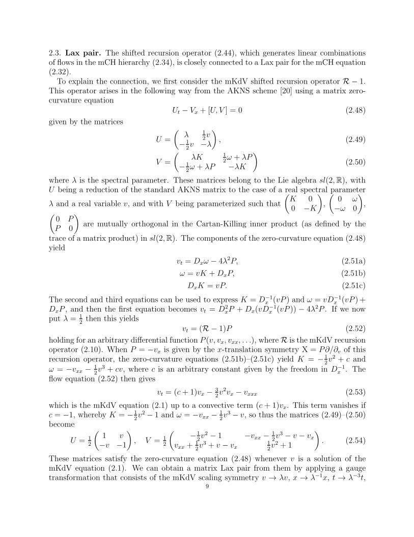
2.3. Lax pair. The shifted recursion operator (2.44), which generates linear combinationsof flows in the mCH hierarchy (2.34), is closely connected to a Lax pair for the mCH equation(2.32).

To explain the connection, we first consider the mKdV shifted recursion operator R− 1.This operator arises in the following way from the AKNS scheme [20] using a matrix zero-curvature equation

Ut − Vx + [U, V ] = 0 (2.48)

given by the matrices

U =

(λ 1

2v

−12v −λ

), (2.49)

V =

(λK 1

2ω + λP

−12ω + λP −λK

)(2.50)

where λ is the spectral parameter. These matrices belong to the Lie algebra sl(2,R), withU being a reduction of the standard AKNS matrix to the case of a real spectral parameter

λ and a real variable v, and with V being parameterized such that

(K 00 −K

),

(0 ω−ω 0

),

(0 PP 0

)are mutually orthogonal in the Cartan-Killing inner product (as defined by the

trace of a matrix product) in sl(2,R). The components of the zero-curvature equation (2.48)yield

vt = Dxω − 4λ2P, (2.51a)

ω = vK +DxP, (2.51b)

DxK = vP. (2.51c)

The second and third equations can be used to express K = D−1x (vP ) and ω = vD−1

x (vP ) +DxP , and then the first equation becomes vt = D2

xP + Dx(vD−1x (vP )) − 4λ2P . If we now

put λ = 12then this yields

vt = (R− 1)P (2.52)

holding for an arbitrary differential function P (v, vx, vxx, . . .), whereR is the mKdV recursionoperator (2.10). When P = −vx is given by the x-translation symmetry X = P∂/∂v of thisrecursion operator, the zero-curvature equations (2.51b)–(2.51c) yield K = −1

2v2 + c and

ω = −vxx −12v3 + cv, where c is an arbitrary constant given by the freedom in D−1

x . Theflow equation (2.52) then gives

vt = (c+ 1)vx −32v2vx − vxxx (2.53)

which is the mKdV equation (2.1) up to a convective term (c + 1)vx. This term vanishes ifc = −1, whereby K = −1

2v2 − 1 and ω = −vxx −

12v3 − v, so thus the matrices (2.49)–(2.50)

become

U = 12

(1 v−v −1

), V = 1

2

(−1

2v2 − 1 −vxx −

12v3 − v − vx

vxx +12v3 + v − vx

12v2 + 1

). (2.54)

These matrices satisfy the zero-curvature equation (2.48) whenever v is a solution of themKdV equation (2.1). We can obtain a matrix Lax pair from them by applying a gaugetransformation that consists of the mKdV scaling symmetry v → λv, x → λ−1x, t → λ−3t,

9

combined with the scaling U → λU , V → λ3V . This is easily seen to produce the standardmKdV matrix Lax pair

U = 12

(λ v−v −λ

), V = 1

2

(−1

2λv2 − λ3 −vxx −

12v3 − λ2v − λvx

vxx +12v3 + λ2v − λvx

12λv2 + λ3

)(2.55)

up to a rescaling of the spectral parameter λ.We now use the relation (2.43) between the mKdV recursion operator and the recursion

operator (2.26) of the mCH equation to re-write the flow equation (2.52) coming from thezero-curvature equation. This gives

vt = (R − 1)∆P = (R − 1)P (2.56)

with

P = ∆−1P . (2.57)

Since R(−vx) = P (1) produces the mCH flow (2.31) when D−1x (0) = 0, we consider P = −vx

and, correspondingly, P = −ux. Then the zero-curvature equations (2.51b)–(2.51c) giveK = −1

2(u2 − u2x) + c and ω = −1

2(u2 − u2x)v − uxx + cv, where c = D−1

x (0) is an arbitraryconstant. Hence, the flow equation (2.56) becomes

vt = (R − 1)(−vx) = (c+ 1)vx −12((u2 − u2x)v)x (2.58)

which is the mCH equation (2.32) up to a convective term (c+1)vx. We put c = −1 to makethis term vanish, which yields

K = −12(u2 − u2x)− 1, ω = −1

2(u2 − u2x)v − u. (2.59)

The matrices (2.49)–(2.50) thereby satisfy the zero-curvature equation (2.48) whenever v isa solution of the mCH equation (2.32). In particular, they are given by

U = 12

(1 v−v −1

), V = 1

4

(u2x − u2 − 2 (u2x − u2)v − 2(u+ ux)

(u2 − u2x)v + 2(u− ux) u2 − u2x + 2

). (2.60)

A Lax pair is obtained from these matrices by applying a gauge transformation defined bythe mCH scaling symmetry u → λ−1u, x → x, t → λ2t, combined with the scaling U → U ,V → λ−2V . This yields

U = 12

(1 λv

−λv −1

), (2.61)

V = 14

(u2x − u2 − 2λ−2 λ(u2x − u2)v − 2λ−1(u+ ux)

λ(u2 − u2x)v + 2λ−1(u− ux) u2 − u2x + 2λ−2

), (2.62)

which is the standard mCH matrix Lax pair (up to rescaling of the spectral parameter λ).Thus, we have shown how the AKNS zero-curvature equation can be used to derive the

matrix Lax pair for the mCH equation. This derivation has not appeared previously in theliterature.

An important final remark arises when we compare this Lax pair (2.61)–(2.62) to themKdV Lax pair (2.55). In both of these Lax pairs, U depends linearly on λ, while Vcontains negative powers of λ in the case of the mCH Lax pair but only positive powers ofλ in the case of the mKdV Lax pair. This indicates that the mCH equation can be viewedas a negative flow in the mKdV hierarchy.

10

3. Tri-Hamiltonian splitting in the NLS hierarchy

The tri-Hamiltonian splitting method was originally applied to the NLS hierarchy in Ref.[9]by considering the standard bi-Hamiltonian structure of the NLS equation. However, thisdid not lead to a peakon equation, because the operator ∆ = 1−D2

x did not appear when thesplit Hamiltonian operators were recombined. We will show how to overcome this obstacleby using a third Hamiltonian structure of the NLS equation, which is connected with thefirst higher flow in the NLS hierarchy.

3.1. NLS hierarchy. We begin from the NLS equation

ivt +12|v|2v + vxx = 0 (3.1)

which has the tri-Hamiltonian structure

vt = i(12|v|2v + vxx) = I(δI/δv) = H(δH/δv) = D(δD/δv) (3.2)

where

I = i, (3.3)

H = −Dx − ivD−1x Im v, (3.4)

D = i(D2x + vD−1

x Re vDx + iDxvD−1x Im v) (3.5)

are mutually compatible Hamiltonian operators, with Re and Im viewed as algebraic oper-ators, and where

D =

∫ ∞

−∞

|v|2 dx, (3.6)

H =

∫ ∞

−∞

Im (vvx) dx, (3.7)

I =

∫ ∞

−∞

14|v|4 − |vx|

2 dx (3.8)

are the corresponding Hamiltonians.The two lowest order Hamiltonian operators (3.3)–(3.4) yield the hereditary recursion

operator

R = HI−1 = i(Dx + vD−1x Re v). (3.9)

This operator and all three of the Hamiltonian operators are invariant under x-translationsapplied to v, as well as phase rotations applied to v, corresponding to the invariance of theNLS equation under infinitesimal x-translations and infinitesimal phase rotations, which arerepresented by the symmetry operators X = −vx∂v and X = iv∂v. These operators yield therespective flows

P (1) = −vx, P (0) = iv (3.10)

which are related by the NLS recursion operator (3.9):

P (1) = RP (0). (3.11)

The NLS equation corresponds to a higher flow

vt = −R(−vx) = −R2(iv) = i(12|v|2v + vxx) (3.12)

11

where the square of the recursion operator is given by

R2 = −DI−1 = −(D2x +DxvD

−1x Re v + ivD−1

x Im vDx). (3.13)

Note that the reduction of this operator (3.13) under the reality condition v = v is givenby the negative of the mKdV recursion operator (2.10). Consequently, for comparison withthe mKdV hierarchy, the most natural way to generate higher flows using the NLS recursionoperator (3.9) is by dividing the NLS hierarchy into even and odd flows

P (2n) = (−R2)n(iv), n = 1, 2, . . . (3.14)

P (2n+1) = (−R2)n(−vx), n = 1, 2, . . . (3.15)

which are related byP (2n+1) = RP (2n). (3.16)

Then all of the odd flows (3.15) will admit a real reduction that yields a corresponding flowin the mKdV hierarchy, whereas all of the even flows (3.15) do not possess a real reduction.

Every flow in the NLS hierarchy (3.14)–(3.15) inherits a tri-Hamiltonian structure, due toMagri’s theorem. For the even flows, this structure is given by

P (2n) = I(δE(n)/δv) = H(δH(n−1)/δv) = D(δE(n−1)/δv), n = 1, 2, . . . (3.17)

where the gradients of the Hamiltonians are generated by

δE(n)/δv = (−R∗2)n(v) = Q(2n), n = 0, 1, 2, . . . (3.18)

δH(n)/δv = −(−R∗2)n(ivx) = Q(2n+1) = −R∗Q(2n), n = 0, 1, 2, . . . (3.19)

and where R∗ is the adjoint recursion operator

R∗ = I−1H = (iDx − vD−1x Im v). (3.20)

The odd flows have a similar but enlarged Hamiltonian structure

P (2n+1) = −I(δH(n)/δv) = H(δE(n)/δv) = −D(δH(n−1)/δv) = E(δE(n−1)/δv), n = 1, 2, . . .(3.21)

where

E = −R2H = −(D3

x +DxvD−1x Re vDx + iD2

xvD−1x Im v + ivD−1

x Im vD2x

+ 12iv(|v|2D−1

x Im v +D−1x |v|2Im v)

) (3.22)

is a fourth Hamiltonian operator which is mutually compatible with I, H, D. In particular,the first higher flow in this hierarchy (3.21) is an integrable U(1)-invariant version of themKdV equation given by

vt = R(i(12|v|2v + vxx)) = −R2(−vx) = −vxxx −

32|v|2vx (3.23)

which is the Hirota equation [23]. It possesses the quad-Hamiltonian structure

vt = −vxxx −32|v|2vx = −I(δH(1)/δv) = H(δE(1)/δv) = −D(δH(0)/δv) = E(δE(0)/δv).

(3.24)Its recursion operator is given by the NLS squared recursion operator (3.13).

In the NLS hierarchy, the real reductions of H and E match the mKdV Hamiltonian opera-tors (2.3)–(2.4), while the Hamiltonians E(n), n = 0, 1, 2, . . . match the mKdV Hamiltonians(7.3), (2.16), multiplied by a factor of 2, with the real reduction of the variational derivativeδ/δv = 1

2(δ/δRe v + iδ/δIm v) having a compensating factor of 1/2.

12

The root flow in the NLS hierarchy of even flows (3.17) has the Hamiltonian structure

P (0) = iv = I(δE(0)/δv) (3.25)

while the root flow in the NLS hierarchy of odd flows (3.21) has the bi-Hamiltonian structure

P (1) = −vx = −I(δH(0)/δv) = H(δE(0)/δv). (3.26)

Both of these root flows possess another Hamiltonian structure if, similarly to the mKdVcase, D−1

x (0) is redefined by the addition of some non-zero constant, so that D−1x (0) = c 6= 0.

Then the relations H(0) = −ivD−1x (0) and D(0) = (iv − vx)D

−1x (0) yield the Hamiltonian

structures−P (0) = c−1H(0), P (1) = c−1(H(0)D(0)) (3.27)

where the corresponding Hamiltonians are trivial.Each higher flow in the combined NLS hierarchy corresponds to a higher symmetry op-

erator X(n) = P (n)∂v, n = 1, 2, . . ., all of which represent infinitesimal symmetries that areadmitted by every equation vt = P (n), n = 1, 2, . . ., in the combined hierarchy. The Hamil-tonians E(n), H(n), n = 0, 1, 2, . . ., of the even and odd flows in the combined hierarchycorrespond to conservation laws d

dtH(n) = d

dtE(n) = 0, all of which hold for every equation

vt = P (n), n = 1, 2, . . ., in the combined hierarchy. All of the higher symmetries and higherHamiltonian densities are local expressions in terms of v and its x-derivatives.

Similarly to the mKdV case, the general scaling method [27] shown in the appendix canbe applied to derive the simple scaling formulas

E(n) =

∫ ∞

−∞

e(n) dx, e(n) = 22n+1

D−1x Re

(vDx(−R2)nv

), n = 0, 1, 2, . . . , (3.28)

H(n) =

∫ ∞

−∞

h(n) dx, h(n) = 1n+1

D−1x Im

(vDx(−R2)nvx

), n = 0, 1, 2, . . . . (3.29)

3.2. Hamiltonian triples. Using the preceding preliminaries, we will now proceed withsplitting the second and third NLS Hamiltonian operators (3.4) and (3.5). Under scaling,the second Hamiltonian operator (3.4) splits into two operators

H1 = −Dx, H2 = −ivD−1x Im v (3.30)

which are a compatible Hamiltonian pair. Likewise, the third Hamiltonian operator (3.5)splits into two operators

D1 = iD2x, D2 = i(D−1

x Re vDx + iDxvD−1x Im v) (3.31)

which are a compatible Hamiltonian pair. The first Hamiltonian operator (3.3), which ob-viously cannot be split, is compatible with each of the two pairs (3.30) and (3.31). Hence,this yields two different Hamiltonian triples:

I, H1, H2 (3.32)

andI, D1, D2. (3.33)

In Ref.[9], the first triple (3.32) was used to obtain the compatible Hamiltonian pair

H = I ±H1 = i∓Dx and D = H2 = −ivD−1x Im v, where H = (1±IDx)I factorizes to yield

a symmetric operator Υ = 1± IDx which is the counterpart of the operator ∆ = 1−D2x in

the mKdV case. The NLS root even flow (3.25) can be expressed as a bi-Hamiltonian flow13

with respect to the Hamiltonian operators H and D through the introduction of a potentialu given by v = Υu = u± iux:

P (0) = iv = H(u) = −(c−1)D(0) (3.34)

where u = H(δH(0)/δv) holds for the Hamiltonian

H(0) =

∫ ∞

−∞

Re (vu) dx =

∫ ∞

−∞

(|u|2 ± Im (uxu)) dx. (3.35)

Then, from Magri’s theorem, the hereditary recursion operator R = DH−1 produces theintegrable equation

vt = R(iv) = ±(i12|u|2v), (3.36)

which has a bi-Hamiltonian structure vt = D(δH(0)/δv) = H(δH(1)/δv) coming from R(iv) =

D(u) = H(Υ−1(±12|u|2v)) with u = δH(0)/δv and Υ−1(±1

2|u|2v) = δH(1)/δv. The first

Hamiltonian H(0) is given by expression (3.35), while the second Hamiltonian H(1) can beobtained by applying the variational relation

Υδ

δv=

δ

δu(3.37)

to get δH(1)/δu = ±12|u|2v, which yields

H(1) =

∫ ∞

−∞

±12|u|2Re (uv) dx =

∫ ∞

−∞

12|u|2(|u|2 + Im (uxu)) dx. (3.38)

However, as discussed in Ref.[9], this bi-Hamiltonian equation (3.36) is not a peakon equa-tion, as it does not contain the operator ∆. We add the remark that the NLS root odd flow(3.26) also does not lead to a peakon equation. In particular, the first Hamiltonian operator

H yields

P (1) = −vx = H(−iux) (3.39)

where −iux = δE(0)/δv holds for the Hamiltonian

E(0) =

∫ ∞

−∞

Im (vux) dx =

∫ ∞

−∞

Im (uux) dx. (3.40)

However, another Hamiltonian structure cannot be found for this flow by using the second

Hamiltonian operator D.We will instead make use of the other compatible Hamiltonian pair

H = I − D1 = i(1−D2x), D = D2 = i(vD−1

x Re vDx + iDxvD−1x Im v) (3.41)

where the first operator has the factorization

H = I∆ = ∆I, ∆ = 1−D2x. (3.42)

The corresponding hereditary recursion operator is given by

R = DH−1 = DxvD−1x Re v∆−1 + ivD−1

x Im vDx∆−1. (3.43)

14

Both of the NLS root flows (3.10) have a Hamiltonian structure with respect to the firstHamiltonian operator in the pair (3.41):

P (0) = iv = H(δH(0)/δv), (3.44)

P (1) = −vx = H(δE(0)/δv), (3.45)

with δH(0)/δv = ∆−1v = u and δE(0)/δv = −i∆−1vx = −iux, where the potential u is nowgiven by

v = ∆u = u− uxx (3.46)

and v is referred to as the momentum variable. By using the variational relation (2.21), we

can formulate the previous Hamiltonian gradients as δH(0)/δu = v and δE(0)/δu = −ivx,from which we obtain the Hamiltonians

H(0) =

∫ ∞

−∞

Re (uv) dx =

∫ ∞

−∞

(|u|2 + |ux|2) dx, (3.47)

E(0) =

∫ ∞

−∞

Im (uvx) dx =

∫ ∞

−∞

Im (ux(uxx − u)) dx (3.48)

after integration by parts. The second Hamiltonian operator in the pair (3.41) gives theHamiltonian structure

D(0) = (c1iv + c2vx). (3.49)

if we redefine D−1x (0) by the addition of an arbitrary non-zero constant, similarly to the

mKdV case, so that D−1x (0) = c 6= 0. Note that we have introduced two separate constants

c1 and c2 due to the two separate D−1x terms that occur in D. In this sense, we can view

each of the NLS root flows (3.44)–(3.45) as having a second Hamiltonian structure, P (0) =

iv = c−11 E(0) and P (1) = −vx = −c−1

2 E(0), with a trivial Hamiltonian.

4. U(1)-invariant peakon equations

We will now explicitly show that the recursion operator (3.43) obtained from splitting thethird Hamiltonian structure of the NLS equation generates a bi-Hamiltonian equation whenit is applied to each of the root flows (3.44)–(3.45) in the NLS hierarchy, with u defined tobe the peakon potential (3.46). This will yield two U(1)-invariant peakon equations.

From the even root flow (3.44), we obtain the first higher flow

P (0,1) = R(iv) = i(12(|u|2 − |u2x|)v + i(Im (uux)v)x

)(4.1)

where R = DH−1 is the recursion operator (3.43), and where D, H are the recombinedHamiltonian operators (3.41). The bi-Hamiltonian structure of this flow (4.1) arises from

R(iv) = D(∆−1v) = H(∆−1(12(|u|2 − |u2x|)v + i(Im (uux)v)x)) (4.2)

in accordance with Magri’s theorem, by expressing

∆−1v = δH(0)/δv (4.3)

and

∆−1(12(|u|2 − |u2x|)v + i(Im (uux)v)x) = δH(1)/δv (4.4)

15

with v = ∆u. These two gradients have an alternative formulation

δH(0)/δu = v, (4.5)

δH(1)/δu = 12(|u|2 − |u2x|)v + i(Im (uux)v)x (4.6)

through the variational identity (2.21). We remark that existence of the Hamiltonians H(0)

and H(1) requires that the right-hand side of each gradient expression (4.5)–(4.6) satisfiesthe Helmholtz conditions [24], as explained in the appendix. The first gradient (4.5) yieldsthe same Hamiltonian appearing in the Hamiltonian structure (3.44) of the even root flow:

H(0) =

∫ ∞

−∞

Re (uv) dx =

∫ ∞

−∞

|u|2 + |ux|2 dx. (4.7)

For the second gradient (4.6), we can straightforwardly verify that the Helmholtz conditionshold by a direct computation, with v = ∆u. Then, since this gradient is given by a homo-geneous expression under scaling of u, we can obtain the Hamiltonian by using the scalingformula shown in the appendix. This yields

H(1) =

∫ ∞

−∞

12Re

(u(1

2(|u|2 − |u2x|)v + i(Im (uux)v)x)

)dx

=

∫ ∞

−∞

14(|u|4 − |ux|

4) + 12Re (u2xuv) dx

(4.8)

modulo boundary terms. Hence, the flow (4.1) has the bi-Hamiltonian structure

P (0,1) = D(δH(0)/δv) = H(δH(1)/δv). (4.9)

The corresponding flow equation vt = P (0,1) is given by

ivt + i(Im (uux)v)x +12(|u|2 − |u2x|)v = 0 (4.10)

which is a NLS-type peakon equation, with the bi-Hamiltonian formulation

vt =12i(|u|2 − |u2x|)v − (Im (uux)v)x = D(δH(0)/δv) = H(δH(1)/δv). (4.11)

Similarly, from the odd root flow (3.45), we obtain the first higher flow

P (1,1) = R(−vx) = D(iux) = −12((|u|2 − |u2x|)v)x − iIm (uux)v. (4.12)

The bi-Hamiltonian structure of this flow (4.12) arises from

R(−vx) = D(i∆−1vx) = H(∆−1(i12((|u|2 − |u2x|)v)x − Im (uux)v)) (4.13)

by expressing i∆−1vx and i12((|u|2 − |u2x|)v)x − Im (uux)v in the gradient form

δE(0)/δu = ivx, (4.14)

δE(1)/δu = i12((|u|2 − |u2x|)v)x − Im (uux)v (4.15)

through the variational identity (2.21). As in the case of the previous flow, existence of

the Hamiltonians E(0) and E(1) requires that the right-hand side of each gradient expres-sion (4.14)–(4.15) satisfies the Helmholtz conditions. The first gradient (4.14) yields theHamiltonian that appears in the Hamiltonian structure (3.45) of the odd root flow:

E(0) =

∫ ∞

−∞

Im (uxv) dx =

∫ ∞

−∞

Im (ux(uxx − u)) dx. (4.16)

16

For the second gradient (4.15), we can straightforwardly verify that the Helmholtz condi-tions hold by a direct computation, with v = ∆u. Then, since this gradient is given by ahomogeneous expressions under scaling of u, we can obtain the Hamiltonian by using thescaling formula shown in the appendix. This yields

E(1) =

∫ ∞

−∞

12Re

(u(i1

2((|u|2 − |u2x|)v)x − Im (uux)v)

)dx

= −

∫ ∞

−∞

34|u|2Im (uux) +

14(2|u|2 − |ux|

2)Im (uxuxx) dx

(4.17)

modulo boundary terms. Hence, the flow (4.12) has the bi-Hamiltonian structure

P (1,1) = D(δE(0)/δv) = H(δE(1)/δv). (4.18)

The corresponding flow equation vt = P (1,1) is given by

vt +12((|u|2 − |u2x|)v)x + iIm (uux)v = 0 (4.19)

which is a Hirota-type peakon equation, with the bi-Hamiltonian formulation

vt = −12((|u|2 − |u2x|)v)x − iIm (uux)v = D(δE(0)/δv) = H(δE(1)/δv). (4.20)

Both of these peakon equations (4.10) and (4.19) are invariant under phase rotations

v → eiφv, φ = const. (4.21)

generated by X = iv∂v, where u = ∆−1v transforms in the same way as v.Under the reality condition v = v, the first peakon equation (4.10) becomes trivial, while

the second peakon equation (4.19) reduces to the mCH peakon equation (2.32).These two peakon equations (4.10) and (4.19) can be formulated as 2-component integrable

systems by decomposing u and v into their real and imaginary parts:

u = u1 + iu2, v = v1 + iv2 (4.22)

withu1 = Reu, u2 = Im u, v1 = Re v, v2 = Im v. (4.23)

Then, the NLS-type peakon equation (4.10) is equivalent to the integrable system

v1t + Av2 + (Bv1)x = 0, v2t − Av1 + (Bv2)x = 0 (4.24)

and the Hirota-type peakon equation (4.19) is equivalent to the integrable system

v1t + (Av1)x −Bv2 = 0, v2t + (Av2)x +Bv1 = 0 (4.25)

whereA = 1

2(u21 + u22 − (u1x)

2 − (u2x)2), B = u1u2x − u2u1x. (4.26)

Each of these integrable systems is invariant under SO(2) rotations on (v1, v2), with (u1, u2)transforming the same way.

Any linear combination of the U(1)-invariant bi-Hamiltonian peakon equations (4.10) and(4.19) is again a U(1)-invariant bi-Hamiltonian peakon equation

vt = −c1((Av)x + iBv) + ic2(Av + i(Bv)x)

= D(δ(c1E(0) + c2H

(0))/δv) = H(δ(c1E(1) + c2H

(1))/δv)(4.27)

withA = 1

2(|u|2 − |ux|

2), B = Im (uux) (4.28)17

where c1, c2 are arbitrary real constants. An equivalent form of this peakon equation (4.27)is given by

vt = c1((A+B)v)x + c2i(A+B)v

= −D(δ(12(c1 + c2)E

(0) + 12(c1 − c2)H

(0))/δv

)

= −H(δ(12(c1 + c2)E

(1) + 12(c1 − c2)H

(1))/δv

)(4.29)

where c1, c2 are arbitrary real constants.We will conclude this derivation by pointing out a simple relationship between the re-

cursion operator (3.43) used in obtaining the U(1)-invariant peakon equations (4.10) and(4.19), and the NLS recursion operator (3.9). First, we express the split Hamiltonian oper-ators (3.31) in terms of the recombined Hamiltonian operators (3.41) by

D1 = (1−∆)I, D2 = D. (4.30)

Next, we substitute these operator expressions into the NLS squared recursion operator(3.13), which is also the recursion operator of the Hirota equation (3.23). This yields

−R2 = DI−1 = D1I−1 +D2I

−1 (4.31)

where

D1I−1 = 1−∆, D2I

−1 = DH−1∆ = R∆. (4.32)

Then, we combine these two equations (4.31)–(4.32) to get the relation

−(R2 + 1) = (R − 1)∆. (4.33)

Since R is a hereditary recursion operator, so is R − 1, and therefore

R = −(R2 + 1)∆−1 (4.34)

defines a hereditary recursion operator, where the hereditary property (2.8) can be checkedto hold directly, without the need for splitting the NLS Hamiltonian operators.

The NLS-type peakon equation (4.10) arises from applying this recursion operator (4.34)to the even root flow (3.44), giving

P (0,1) = R(iv) = −(R2 + 1)(iu) (4.35)

where

R2(iu) = i(−uxx −12(u2 − u2x)v + i(Im (uxu)v)x). (4.36)

Hence, we have

P (0,1) = −(R2 + 1)(iu) = −iv + 12i(|u|2 − |u2x|)v − (Im (uux)v)x = P (0,1) − P (0) (4.37)

which is a linear combination of the root flow (3.44) and the NLS-type peakon flow (4.10).Since both of those flows possess a bi-Hamiltonian structure given by the pair of Hamiltonianoperators (3.41), the resulting flow (4.37) is also bi-Hamiltonian. The corresponding bi-

Hamiltonian equation vt = P (0,1) is a slight generalization of the NLS-type peakon equation(4.10):

ivt − v + i(Im (uux)v)x +12(|u|2 − |u2x|)v = 0. (4.38)

In particular, a phase transformation v → v = e−itv applied to the NLS-type peakon equation(4.10) yields the generalized equation (4.38).

18

In a similar way, the Hirota-type peakon equation (4.19) arises from applying the recursionoperator (4.34) to the odd root flow (3.45), giving

P (1,1) = R(−vx) = −(R2 + 1)(−ux) (4.39)

where

R2(−ux) = uxxx +12((u2 − u2x)v)x + iIm (uxu)v. (4.40)

This yields a linear combination of the root flow (3.45) and the Hirota-type peakon flow(4.19),

P (1,1) = −(R2 + 1)(−ux) = vx −12((|u|2 − |u2x|)v)x + iIm (uux)v = P (1,1) − P (1) (4.41)

which is a bi-Hamiltonian flow with respect to the pair of Hamiltonian operators (3.41). The

corresponding bi-Hamiltonian equation vt = P (1,1) is a slight generalization of the Hirota-type peakon equation (4.19):

vt − vx +12((|u|2 − |u2x|)v)x − iIm (uux)v = 0. (4.42)

In particular, a Galilean transformation x→ x = x+ t, t→ t = t applied to the Hirota-typepeakon equation (4.19) yields the generalized equation (4.42).

Finally, although the two root flows (3.44) and (3.45) are related by the NLS recursionoperator (3.9), the same relation does not hold for the two U(1)-invariant peakon flows (4.37)

and (4.41), since −ux −R(iu) = −iIm (uxu)v 6= 0 shows that P (1,1) 6= RP (0,1).

5. Integrability properties

We will now derive some further aspects of the integrability structure of the two U(1)-invariant peakon equations (4.10) and (4.19), specifically, their hierarchies of symmetries andconservation laws, and their Lax pairs.

5.1. Symmetries. The recursion operator (3.43) which generates the U(1)-invariant peakonequations (4.10) and (4.19) by applying it to the even and odd root flows (3.10) in the NLShierarchy is invariant under x-translations and U(1)-phase rotations. Consequently, from a

standard result in the theory of recursion operators [26, 24], this operator R gives rise totwo hierarchies of flows

P (0,n) = Rn(iv), n = 1, 2, . . . , (5.1)

P (1,n) = Rn(−vx), n = 1, 2, . . . , (5.2)

starting from the two NLS root flows P (0) = iv and P (1) = −vx, where the n = 1 flowscorrespond to the respective U(1)-invariant peakon equations (4.10) and (4.19), as given by

vt = P (0,1) = 12i(|u|2 − |u2x|)v − (Im (uux)v)x, (5.3)

vt = P (1,1) = −12((|u|2 − |u2x|)v)x − iIm (uux)v. (5.4)

Every flow in these two hierarchies is invariant under x-translations and U(1)-phase rotations.These two symmetries are respectively generated by

Xtrans. = −vx∂/∂v, Xphas. = iv∂/∂v. (5.5)19

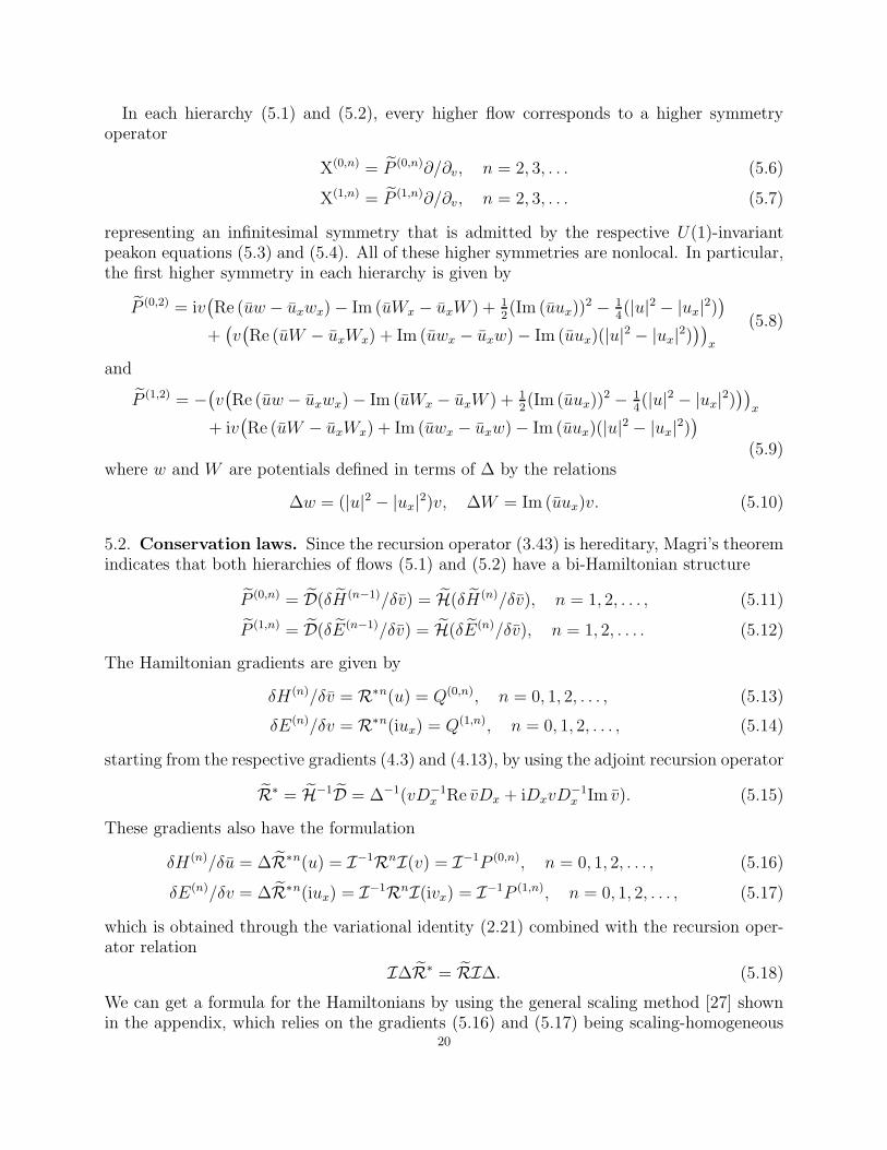
In each hierarchy (5.1) and (5.2), every higher flow corresponds to a higher symmetryoperator

X(0,n) = P (0,n)∂/∂v, n = 2, 3, . . . (5.6)

X(1,n) = P (1,n)∂/∂v, n = 2, 3, . . . (5.7)

representing an infinitesimal symmetry that is admitted by the respective U(1)-invariantpeakon equations (5.3) and (5.4). All of these higher symmetries are nonlocal. In particular,the first higher symmetry in each hierarchy is given by

P (0,2) = iv(Re (uw − uxwx)− Im (uWx − uxW ) + 1

2(Im (uux))

2 − 14(|u|2 − |ux|

2))

+(v(Re (uW − uxWx) + Im (uwx − uxw)− Im (uux)(|u|

2 − |ux|2)))

x

(5.8)

and

P (1,2) = −(v(Re (uw − uxwx)− Im (uWx − uxW ) + 1

2(Im (uux))

2 − 14(|u|2 − |ux|

2)))

x

+ iv(Re (uW − uxWx) + Im (uwx − uxw)− Im (uux)(|u|

2 − |ux|2))

(5.9)where w and W are potentials defined in terms of ∆ by the relations

∆w = (|u|2 − |ux|2)v, ∆W = Im (uux)v. (5.10)

5.2. Conservation laws. Since the recursion operator (3.43) is hereditary, Magri’s theoremindicates that both hierarchies of flows (5.1) and (5.2) have a bi-Hamiltonian structure

P (0,n) = D(δH(n−1)/δv) = H(δH(n)/δv), n = 1, 2, . . . , (5.11)

P (1,n) = D(δE(n−1)/δv) = H(δE(n)/δv), n = 1, 2, . . . . (5.12)

The Hamiltonian gradients are given by

δH(n)/δv = R∗n(u) = Q(0,n), n = 0, 1, 2, . . . , (5.13)

δE(n)/δv = R∗n(iux) = Q(1,n), n = 0, 1, 2, . . . , (5.14)

starting from the respective gradients (4.3) and (4.13), by using the adjoint recursion operator

R∗ = H−1D = ∆−1(vD−1x Re vDx + iDxvD

−1x Im v). (5.15)

These gradients also have the formulation

δH(n)/δu = ∆R∗n(u) = I−1RnI(v) = I−1P (0,n), n = 0, 1, 2, . . . , (5.16)

δE(n)/δv = ∆R∗n(iux) = I−1RnI(ivx) = I−1P (1,n), n = 0, 1, 2, . . . , (5.17)

which is obtained through the variational identity (2.21) combined with the recursion oper-ator relation

I∆R∗ = RI∆. (5.18)

We can get a formula for the Hamiltonians by using the general scaling method [27] shownin the appendix, which relies on the gradients (5.16) and (5.17) being scaling-homogeneous

20

expressions of u and x-derivatives of u. This yields

H(n) =

∫ ∞

−∞

h(n) dx, h(n) = 1n+1

Im (uP (0,n)), (5.19)

E(n) =

∫ ∞

−∞

e(n) dx, e(n) = 1n+1

Im (uP (1,n)) (5.20)

modulo boundary terms. All of the higher Hamiltonian densities are nonlocal. In particular,the first higher density in each hierarchy is given by

h(2) = −13

(Re (uv)

(Re (uw − uxwx)− Im (uWx − uxW ) + 1

2(Im (uux))

2 − 14(|u|2 − |ux|

2))

+ Im (uxv)(Re (uW − uxWx) + Im (uwx − uxw)− Im (uux)(|u|

2 − |ux|2)))

(5.21)and

e(2) = 13

(Im (uxv)

(Re (uw − uxwx)− Im (uWx − uxW ) + 1

2(Im (uux))

2 − 14(|u|2 − |ux|

2))

− Re (uv)(Re (uW − uxWx) + Im (uwx − uxw)− Im (uux)(|u|

2 − |ux|2)))

(5.22)where w and W are the potentials (5.10).

5.3. Lax pair. The recursion operator (3.43) generating the two hierarchies of U(1)-invariant peakon flows (5.1)–(5.2) can be derived similarly to the mCH recursion operatorby using a matrix zero-curvature equation (2.48) based on the AKNS scheme. Here thezero-curvature matrices are taken to have the form

U =

(λ 1

2v

−12v −λ

), (5.23)

V =

(λK + 1

2iJ 1

2ω + λP

−12ω + λP −λK − 1

2iJ

), (5.24)

belonging to the Lie algebra sl(2,C), where K and J are real functions, and where Pand ω are complex functions. Note that U is the standard AKNS matrix, but with the

spectral parameter λ being real, and V is parameterized such that

(K 00 −K

),

(iJ 00 −iJ

),

(0 ω−ω 0

),

(0 PP 0

)are mutually orthogonal in the Cartan-Killing inner product in sl(2,C).

(Recall, this inner product is defined by the trace of the product of a sl(2,C) matrix and ahermitian conjugated sl(2,C) matrix.) In this representation, the components of the zero-curvature equation (2.48) yield

vt = Dxω + iJv − 4λ2P, (5.25a)

ω = Kv +DxP, (5.25b)

DxK = Re (vP ), (5.25c)

DxJ = Im (vω). (5.25d)

Equations (5.25b)–(5.25c) can be used to express K = D−1x Re (vP ) and ω = vD−1

x Re (vP )+DxP , and equation (5.25d) then gives J = D−1

x Im (vω) = D−1x Im (vDxP ), which yields

21

vt = D2xP +Dx(vD

−1x Re (vP )) + ivD−1

x Im (vDxP )− 4λ2P from equation (5.25a). If we nowput λ = 1

2then we obtain

vt = −(R2 + 1)P (5.26)

holding for an arbitrary differential function P (v, vx, vxx, . . .), where R is the NLS recursionoperator (3.9) and −R2 is the recursion operator (3.13) that generates the even flows (3.14)and the odd flows (3.15) in the NLS hierarchy. This shows that, in the matrices (5.23)–(5.24),P can be identified with the generator of any flow in the NLS hierarchy.

As a first step to obtain a Lax pair in a systematic way, we will show how to use thesematrices (5.23)–(5.24) to derive a Lax pair for the root flows in each of the two hierarchies(3.14) and (3.15).

In particular, for P = iv, which corresponds to the even root flow in the NLS hierarchy,the zero-curvature equations (5.25b)–(5.25d) yield K = c1, ω = ivx + c1v, J = 1

2|v|2 + c2,

where c1, c2 are arbitrary constants given by the freedom in D−1x . The flow equation (5.26)

then produces the NLS equation (3.1) if we choose c1 = 0 and c2 = −1. Consequently,substitution of

K = 0, ω = ivx, J = 12|v|2 − 1 (5.27)

into these matrices (5.23)–(5.24), followed by a gauge transformation consisting of the NLSscaling symmetry v → λv, x → λ−1x, t → λ−2t combined with the scaling U → λU ,V → λ2V , can be seen to give the standard NLS matrix Lax pair

U = 12

(λ v−v −λ

), V = 1

2i

(12|v|2 + λ2 vx + λvvx − λv −1

2|v|2 − λ2

)(5.28)

up to rescaling the spectral parameter. Likewise, for P = −vx, which corresponds to theodd root flow in the NLS hierarchy, the zero-curvature equations (5.25b)–(5.25d) yield K =−1

2|v|2 + c1, ω = −vxx −

12|v|2v + c1v, J = Im (vxv) + c2. If we now choose c1 = −1 and

c2 = 0, then the flow equation (5.26) produces the Hirota equation (3.23). Substitution of

K = −12|v|2 − 1, ω = −vxx −

12|v|2v − v, J = Im (vxv) (5.29)

into the matrices (5.23)–(5.24), followed by a gauge transformation v → λv, x → λ−1x,t→ λ−3t, U → λU , V → λ3V , thereby gives a matrix Lax pair for the Hirota equation

U = 12

(λ v−v −λ

), V = 1

2

(iIm (vxv)−

12λ|v|2 − λ3 −vxx −

12|v|2v − λ2v − λvx

vxx +12|v|2v + λ2v − λvx −iIm (vxv) +

12λ|v|2 + λ3

)

(5.30)up to rescaling the spectral parameter.

We will next adapt the previous steps to both the NLS-type peakon equation (4.10) andthe Hirota-type peakon equation (4.19). The main idea is to use the NLS recursion operatorrelation (4.33) to express the zero-curvature flow equation (5.26) in terms of the recursion

operator R that generates the two hierarchies of U(1)-invariant peakon flows (5.1)–(5.2).This yields

vt = (R − 1)∆P = (R − 1)P (5.31)

with

P = ∆−1P . (5.32)22

As a result, P can be chosen to be the generator of any flow in the hierarchies (5.1)–(5.2).We proceed by separately considering the two flows

P (0,0) = iv, P (1,0) = −vx (5.33)

which are the respective (n = 0) root flows in these two hierarchies. The corresponding flowson the potential u are given by

P (0,0) = iu, P (1,0) = −ux. (5.34)

For the first flow P = P (0,0) = iu, the zero-curvature equations (5.25b)–(5.25d) giveK = Im (uxu) + c1, ω = Im (uxu)v + c1v + iux, J = 1

2(|u|2 − |ux|

2) + c2. Hence, the flowequation (5.31) becomes

vt = (R − 1)(iv) = i(c2 − 1)v + c1vx +12i(|u|2 − |ux|

2)v + (Im (uxu)v)x (5.35)

which is the NLS-type peakon equation (4.10) if we put c2 = 1 and c1 = 0. Then, bysubstituting

K = Im (uxu), ω = Im (uxu)v + iux, J = 12(|u|2 − |ux|

2) + 1 (5.36)

into the matrices (5.23)–(5.24), and applying a gauge transformation given by

u→ λ−1u, x→ x, t→ λ2t, U → U, V → λ−2V, (5.37)

we obtain the Lax pair

U = 12

(1 λv

−λv −1

), (5.38)

V = 14

(i(|u|2 − |ux|

2) + 2Im (uxu) + 2iλ−2 2λIm (uxu)v + 2iλ−1(u+ ux)−2λIm (uxu)v − 2iλ−1(u− ux) i(|ux|

2 − |u|2)− 2Im (uxu)− 2iλ−2

). (5.39)

For the second flow P = P (1,0) = −ux, the zero-curvature equations (5.25b)–(5.25d) giveK = −1

2(|u|2 − |ux|

2) + c1, ω = −12(|u|2 − |ux|

2)v + c1v− uxx, J = Im (uxu) + c2. Hence, theflow equation (5.31) becomes

vt = (R − 1)(iv) = ic2v + (c1 + 1)vx −12((|u|2 − |ux|

2)v)x + iIm (uxu)v (5.40)

which is the Hirota-type peakon equation (4.19) if we put c1 = −1 and c2 = 0. Then, bysubstituting

K = −12(|u|2 − |ux|

2)− 1, ω = −12(|u|2 − |ux|

2)v − u, J = Im (uxu) (5.41)

into the matrices (5.23)–(5.24), and applying the gauge transformation (5.37), we obtain theLax pair

U = 12

(1 λv

−λv −1

), (5.42)

V = 14

(|ux|

2 − |u|2 + 2iIm (uxu)− 2λ−2 λ(|ux|2 − |u|2)v − 2λ−1(u+ ux)

λ(|u|2 − |ux|2)v + 2λ−1(u− ux) |u|2 − |ux|

2 − 2iIm (uxu) + 2λ−2

). (5.43)

Comparing the NLS Lax pair (5.28) to these two Lax pairs (5.38)–(5.39) and (5.42)–(5.43),we see that U depends linearly on λ while V contains negative powers of λ in the case ofthe peakon equations but only positive powers of λ in the case of the NLS equation. Thisindicates that the two peakon equations can be viewed as negative flows in the NLS hierarchy.

23

6. Peakon solutions

A peakon u(t, x) is a peaked travelling wave

u = a exp(−|x− ct|), a, c = const. (6.1)

where the amplitude a and the speed c are related by some algebraic equation. This ex-pression (6.1) is motivated by the form of the kernel of the operator ∆ = 1 − ∂2x. Thecorresponding momentum variable (3.46) is a distribution

v = u− uxx = 2aδ(x− ct). (6.2)

Peakons are not classical solutions and instead are commonly understood as weak solutions[28, 29, 30, 31, 32, 16] in the setting of an integral (weak) formulation of a given peakonequation. A weak formulation is defined by multiplying the peakon equation by test functionψ(t, x) and integrating by parts to remove all terms involving v and derivatives of v, leavingat most u, ux, and ut in the integral. The weak formulation of the mCH equation (2.32) isgiven by

0 =

∫∫

R2

((ψ − ψxx)ut + (3ψ − ψxx)uux −

12ψxu

2x

)dx dt. (6.3)

Its well-known peakon solution [13, 16] has the amplitude-speed relation a = c:

u = c exp(−|x− ct|), c = const. (6.4)

For both the NLS-type peakon equation (5.3) and the Hirota-type peakon equation (5.4),their U(1)-invariance allows for the possibility of oscillatory peakon solutions whose form isgiven by a peaked travelling wave a exp(−|x − ct|) modulated by an oscillatory plane-wavephase exp(i(φ+ wt+ kx)).

We will begingby considering smooth plane-wave solutions

u = a exp(i(kx+ wt)), a, k, w = const. (6.5)

Substitution of this expression into the Hirota-type peakon equation (5.4) yields

w = 12a2k(k2 − 3) (6.6)

which represents a nonlinear dispersion relation for the plane-wave. Similarly, the NLS-typepeakon equation (5.3) yields

w = 12a2(1− 3k2) (6.7)

which is a different nonlinear dispersion relation. Note the speeds c = −w/k of the resultingplane-waves are respectively given by

c = 12a2(3− k2) (6.8)

andc = 1

2a2(3k2 − 1)/k. (6.9)

In the Hirota case (6.8), the plane-wave has the amplitude-speed form

u = a exp(± i

√3− 2c/a2(x− ct)

)(6.10)

where c ≤ 32a2. This wave can move in either direction but has a maximum speed of

cmax = 32a2 in the positive x direction. In the NLS case (6.8), the amplitude-speed form of

the plane-wave is given by

u = a exp(i13(±

√3 + c2/a4 + c/a2)(x− ct)

). (6.11)

24

This wave can move in either direction, with no restriction on its speed.These features of the plane-wave solutions are analogous to the features of the oscillatory

solitons [33] of the Hirota equation (3.23) and the usual solitons [20] of the NLS equation(3.1).

We will now seek oscillatory peakon solutions

u = a exp(i(φ+ wt+ kx)) exp(−|ξ|), ξ = x− ct, a, c, φ, w, k = const. (6.12)

where w/(2π) is a temporal oscillation frequency, 2π/k is a spatial modulation length, and φis a phase angle. The momentum variable (3.46) corresponding to expression (6.12) is givenby the distribution

v = u− uxx = 2a exp(i(φ+ wt))δ(ξ) + a exp(i(φ+ wt+ kx)− |ξ|)(i2k sgn(ξ) + k2

). (6.13)

To proceed, we first observe that neither of the U(1)-invariant peakon equations (5.3) and(5.4) has a weak formulation that involves only u, u, and their first derivatives. In partic-ular, after multiplication by a complex-valued test function ψ(t, x), the NLS-type equation(5.3) contains problematic terms ψ|ux|

2uxx = 12ψux(u

2x)x and ψ(uxuuxx)x ≡ −ψxuxuuxx,

which cannot be expressed as total x-derivatives (where “≡” denotes equality modulo atotal x-derivative). Likewise the Hirota-type equation (5.4) contains problematic termsψ(|ux|

2uxx)x ≡ −ψxuxuxuxx and ψuxuuxx.But since the oscillatory peakon expression (6.12) factorizes into a standard peakon am-

plitude expression a exp(−|x− ct|) and an oscillatory phase expression exp(i(φ+wt+ kξ)),we can consider a weak formulation in which a polar form

u = A exp(iΦ), u = A exp(−iΦ) (6.14)

is used such that any derivatives of A of second and higher orders are removed. Specifically,first we substitute this polar form into the peakon equations (5.3) and (5.4) multiplied bythe test function ψ(t, x); next we use integration by parts to remove all terms involvingAxx, Atx, and their derivatives; then we split the resulting integral equation into its real andimaginary parts. This yields what we will call a weak-amplitude formulation.

Lemma 1. (i) The NLS-type peakon equation (5.3) in polar form has the weak-amplitudeformulation

0 =

∫∫

R2

(ψ1xx

(At + ΦxA

2Ax

)+ ψ1x

(2ΦxAA

2x + ΦxxA

2Ax

)− ψ1

(At +

56ΦxA

3x

+ 12ΦxxAA

2x +

12(5 + 7Φ2

x)ΦxA2Ax +

12(1 + 7Φ2

x)ΦxxA3))dx dt,

(6.15)

0 =

∫∫

R2

(ψ2xxAΦt − ψ2x

(16A3

x +12(3Φ2

x − 1)A2Ax + ΦxΦxxA3)− ψ2

(12(3Φ2

x − 1)AA2x

+ ΦxΦxxA2Ax −

12(1 + Φ2

x)(1− 3Φ2x)A

3 + ΦtA))dx dt,

(6.16)

where ψ1(t, x), ψ2(t, x) are real test functions. This pair of integral equations (6.15)–(6.16)is satisfied by all classical solutions of the NLS-type peakon equation (5.3).

25

(ii) The Hirota-type equation (5.4) in polar form has the weak-amplitude formulation

0 =

∫∫

R2

(ψ1xx

(16A3

x +12(Φ2

x − 1)A2Ax −At

)+ ψ1x

(12(3Φ2

x − 1)AA2x + ΦxΦxxA

2Ax

)

− ψ1

(12(3Φ4

x − 2Φ2x − 3)A2Ax −At + (2Φ2

x − 1)ΦxΦxxA3))dx dt,

(6.17)

0 =

∫∫

R2

(ψ2xxAΦt + ψ2x

(56ΦxA

3x +

12ΦxxAA

2x +

12(Φ2

x − 3)ΦxA2Ax +

12(Φ2

x − 1)ΦxxA3)

+ ψ2

(2ΦxAA

2x + ΦxxA

2Ax + (Φ2x + 1)(3− Φ2

x)ΦxA3 + ΦtA

))dx dt.

(6.18)

This pair of integral equations (6.17)–(6.18) is satisfied by all classical solutions of the Hirota-type peakon equation (5.4).

All non-smooth solutions (6.14) of these integral equations will be weak-amplitude solutionsof the corresponding peakon equations on the real line, x ∈ R.

To derive the 1-peakon solutions of the NLS-type peakon equation (5.3) and the Hirota-type peakon equation (5.4), we begin by substituting expression (6.12) in polar form A =ae−|ξ|, Φ = φ + wt + kx into the corresponding weak-amplitude integral equations. Next,we change the spatial integration variable from x to ξ and split its integration domain into(−∞, 0) and (0,∞). Finally, we use integration by parts to evaluate the integrals.

6.1. Hirota peakons. The Hirota peakon weak-amplitude integrals (6.17)–(6.18) are re-spectively given by

0 =

∫∫

R2

((cae−|ξ| + 1

2(3k4 − 2k2 − 3)a3e−3|ξ|

)sgn(ξ)ψ1(ξ + ct, t)

+(12(3k2 − 1)a3e−3|ξ|

)ψ1x(ξ + ct, t)

+(16(2− 3k2)a3e−3|ξ| − cae−|ξ|

)sgn(ξ)ψ1xx(ξ + ct, t)

)dξ dt

=

∫∫

R2

(12k2(3k2 − 2)a3e−3|ξ|

)sgn(ξ)ψ1(ξ + ct, t) dξ dt

+ a(2c+ a2k2 − 23a2)

∫

R

ψ1x(ct, t) dt

(6.19)

and

0 =

∫∫

R2

((wae−|ξ| − 1

2k(k4 − 2k2 − 7)a3e−3|ξ|

)ψ2(ξ + ct, t)

+(16k(3k2 − 4)a3e−3|ξ|

)sgn(ξ)ψ2x(ξ + ct, t)−

(wae−|ξ|

)ψ2xx(ξ + ct, t)

)dξ dt

=

∫∫

R2

(12k(3 + 5k2 − k4)a3e−3|ξ|

)ψ2(ξ + ct, t)dξ dt

+ a(2w − 3a2k3 + 43a2k)

∫

R

ψ1(ct, t) dt.

(6.20)26

This pair of equations must hold for all test functions ψ1 and ψ2, respectively. Hence, weobtain the conditions

ak(3k2 − 2) = 0, a(2c+ a2k2 − 23a2) = 0, (6.21)

ak(k4 − 5k2 − 3) = 0, a(2w − 3a2k3 + 43a2k) = 0. (6.22)

We want a 6= 0, and so then these four conditions yield

k = 0, w = 0, c = 13a2. (6.23)

Thus, the 1-peakon solution of the Hirota-type peakon equation (5.4) is given by

u = a exp(iφ− |x− 13a2t|), a, φ = const. (6.24)

which represents a complex-valued peaked travelling wave with a constant phase. In fact,this solution is simply the mCH peakon (6.4) multiplied by the phase eiφ, and its existence isa direct consequence of the Hirota-type peakon equation being U(1)-invariant and reducingto the mCH equation under u = u.

In contrast, the NLS-type peakon equation (5.3) becomes trivial under u = u, and so weexpect that its peakon solution will be qualitatively different than the mCH peakon (6.4)and the Hirota peakon (6.24).

6.2. NLS peakon breathers. The NLS peakon weak-amplitude integrals (6.15)–(6.16) arerespectively given by

0 =

∫∫

R2

((cae−|ξ| − 1

6(21k2 + 20)a3e−3|ξ|

)sgn(ξ)ψ1(ξ + ct, t)

−(2ka3e−3|ξ|

)ψ1x(ξ + ct, t) +

(ka3e−3|ξ| − cae−|ξ|

)sgn(ξ)ψ1xx(ξ + ct, t)

)dξ dt

=−

∫∫

R2

(16k(21k2 + 2)a3e−3|ξ|

)sgn(ξ)ψ1(ξ + ct, t) dξ dt

+ 2a(c− a2k)

∫

R

ψ1x(ct, t) dt

(6.25)and

0 =

∫∫

R2

((wae−|ξ| + 1

2(k2 + 2)(3k2 − 1)a3e−3|ξ|

)ψ2(ξ + ct, t)

+(16(2− 9k2)a3e−3|ξ|

)sgn(ξ)ψ2x(ξ + ct, t)−

(wae−|ξ|

)ψ2xx(ξ + ct, t)

)dξ dt

=

∫∫

R2

(12k2(3k2 − 4)a3e−3|ξ|

)ψ2(ξ + ct, t)dξ dt

+ a(2w + 3a2k2 − 23a2)

∫

R

ψ2(ct, t) dt.

(6.26)Since this pair of equations must hold for all test functions ψ1 and ψ2, we obtain the respectiveconditions

ak(21k2 + 2) = 0, a(c− a2k) = 0, (6.27)

ak(3k2 − 4) = 0, a(2w + 3a2k2 − 23a2) = 0, (6.28)

27

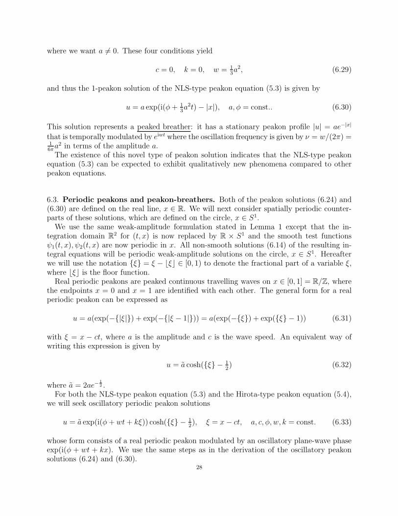
where we want a 6= 0. These four conditions yield

c = 0, k = 0, w = 13a2, (6.29)

and thus the 1-peakon solution of the NLS-type peakon equation (5.3) is given by

u = a exp(i(φ+ 13a2t)− |x|), a, φ = const.. (6.30)

This solution represents a peaked breather: it has a stationary peakon profile |u| = ae−|x|

that is temporally modulated by eiwt where the oscillation frequency is given by ν = w/(2π) =16πa2 in terms of the amplitude a.The existence of this novel type of peakon solution indicates that the NLS-type peakon

equation (5.3) can be expected to exhibit qualitatively new phenomena compared to otherpeakon equations.

6.3. Periodic peakons and peakon-breathers. Both of the peakon solutions (6.24) and(6.30) are defined on the real line, x ∈ R. We will next consider spatially periodic counter-parts of these solutions, which are defined on the circle, x ∈ S1.

We use the same weak-amplitude formulation stated in Lemma 1 except that the in-tegration domain R

2 for (t, x) is now replaced by R × S1 and the smooth test functionsψ1(t, x), ψ2(t, x) are now periodic in x. All non-smooth solutions (6.14) of the resulting in-tegral equations will be periodic weak-amplitude solutions on the circle, x ∈ S1. Hereafterwe will use the notation {ξ} = ξ − ⌊ξ⌋ ∈ [0, 1) to denote the fractional part of a variable ξ,where ⌊ξ⌋ is the floor function.

Real periodic peakons are peaked continuous travelling waves on x ∈ [0, 1] = R/Z, wherethe endpoints x = 0 and x = 1 are identified with each other. The general form for a realperiodic peakon can be expressed as

u = a(exp(−{|ξ|}) + exp(−{|ξ − 1|})) = a(exp(−{ξ}) + exp({ξ} − 1)) (6.31)

with ξ = x − ct, where a is the amplitude and c is the wave speed. An equivalent way ofwriting this expression is given by

u = a cosh({ξ} − 12) (6.32)

where a = 2ae−1

2 .For both the NLS-type peakon equation (5.3) and the Hirota-type peakon equation (5.4),

we will seek oscillatory periodic peakon solutions

u = a exp(i(φ+ wt+ kξ)) cosh({ξ} − 12), ξ = x− ct, a, c, φ, w, k = const. (6.33)

whose form consists of a real periodic peakon modulated by an oscillatory plane-wave phaseexp(i(φ + wt + kx). We use the same steps as in the derivation of the oscillatory peakonsolutions (6.24) and (6.30).

28

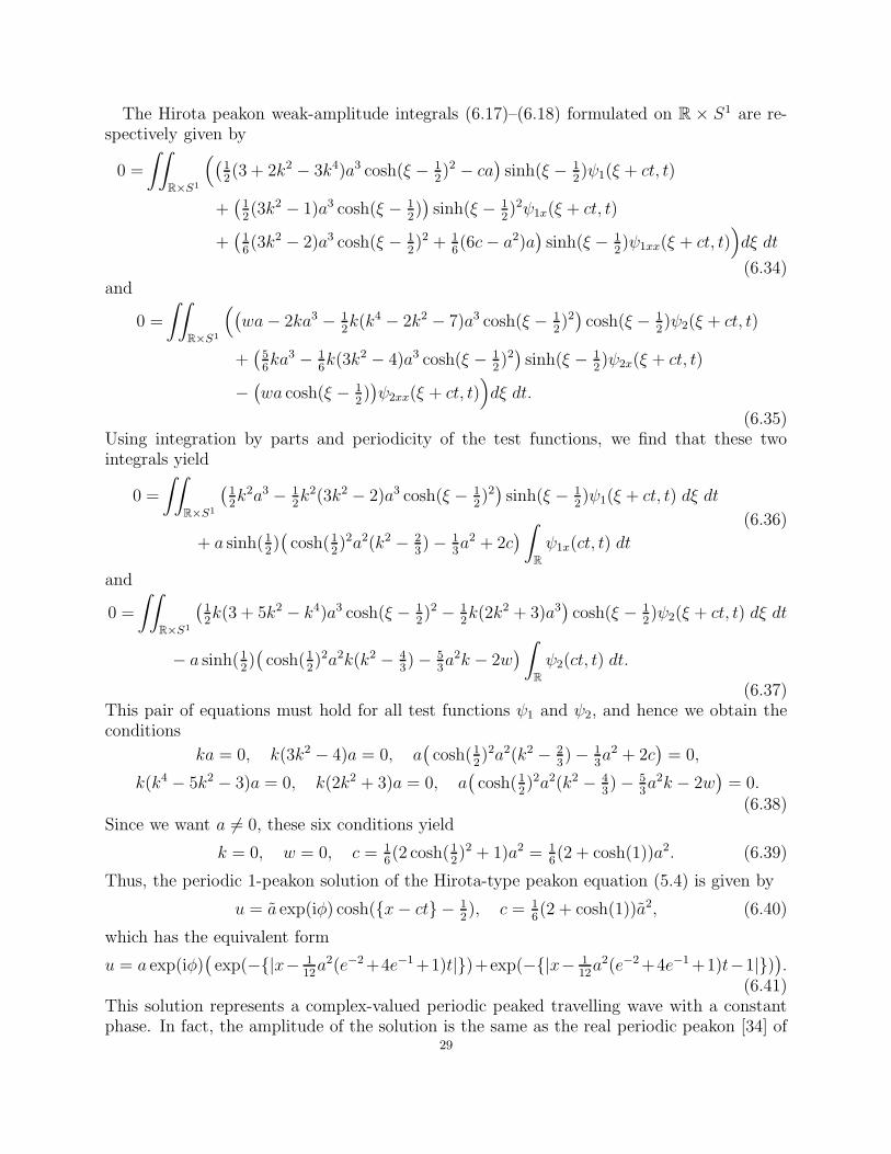
The Hirota peakon weak-amplitude integrals (6.17)–(6.18) formulated on R × S1 are re-spectively given by

0 =

∫∫

R×S1

((12(3 + 2k2 − 3k4)a3 cosh(ξ − 1

2)2 − ca

)sinh(ξ − 1

2)ψ1(ξ + ct, t)

+(12(3k2 − 1)a3 cosh(ξ − 1

2))sinh(ξ − 1

2)2ψ1x(ξ + ct, t)

+(16(3k2 − 2)a3 cosh(ξ − 1

2)2 + 1

6(6c− a2)a

)sinh(ξ − 1

2)ψ1xx(ξ + ct, t)

)dξ dt

(6.34)and

0 =

∫∫

R×S1

((wa− 2ka3 − 1

2k(k4 − 2k2 − 7)a3 cosh(ξ − 1

2)2)cosh(ξ − 1

2)ψ2(ξ + ct, t)

+(56ka3 − 1

6k(3k2 − 4)a3 cosh(ξ − 1

2)2)sinh(ξ − 1

2)ψ2x(ξ + ct, t)

−(wa cosh(ξ − 1

2))ψ2xx(ξ + ct, t)

)dξ dt.

(6.35)Using integration by parts and periodicity of the test functions, we find that these twointegrals yield

0 =

∫∫

R×S1

(12k2a3 − 1

2k2(3k2 − 2)a3 cosh(ξ − 1

2)2)sinh(ξ − 1

2)ψ1(ξ + ct, t) dξ dt

+ a sinh(12)(cosh(1

2)2a2(k2 − 2

3)− 1

3a2 + 2c

) ∫

R

ψ1x(ct, t) dt

(6.36)

and

0 =

∫∫

R×S1

(12k(3 + 5k2 − k4)a3 cosh(ξ − 1

2)2 − 1

2k(2k2 + 3)a3

)cosh(ξ − 1

2)ψ2(ξ + ct, t) dξ dt

− a sinh(12)(cosh(1

2)2a2k(k2 − 4

3)− 5

3a2k − 2w

) ∫

R

ψ2(ct, t) dt.

(6.37)This pair of equations must hold for all test functions ψ1 and ψ2, and hence we obtain theconditions

ka = 0, k(3k2 − 4)a = 0, a(cosh(1

2)2a2(k2 − 2

3)− 1

3a2 + 2c

)= 0,

k(k4 − 5k2 − 3)a = 0, k(2k2 + 3)a = 0, a(cosh(1

2)2a2(k2 − 4

3)− 5

3a2k − 2w

)= 0.(6.38)

Since we want a 6= 0, these six conditions yield

k = 0, w = 0, c = 16(2 cosh(1

2)2 + 1)a2 = 1

6(2 + cosh(1))a2. (6.39)

Thus, the periodic 1-peakon solution of the Hirota-type peakon equation (5.4) is given by

u = a exp(iφ) cosh({x− ct} − 12), c = 1

6(2 + cosh(1))a2, (6.40)

which has the equivalent form

u = a exp(iφ)(exp(−{|x− 1

12a2(e−2+4e−1+1)t|})+exp(−{|x− 1

12a2(e−2+4e−1+1)t−1|})

).

(6.41)This solution represents a complex-valued periodic peaked travelling wave with a constantphase. In fact, the amplitude of the solution is the same as the real periodic peakon [34] of

29

the mCH equation (2.32), which is a direct consequence of the Hirota-type peakon equationreducing to the mCH equation under u = u.

The NLS peakon weak-amplitude integrals (6.15)–(6.16) formulated on R×S1 are respec-tively given by

0 =

∫∫

R×S1

((16(21k + 20)a3 cosh(ξ − 1

2)2 − 1

6(5ka2 + 6c)a

)sinh(ξ − 1

2)ψ1(ξ + ct, t)

−(2ka3 cosh(ξ − 1

2) sinh(ξ − 1

2)2)ψ1x(ξ + ct, t)

+(ca− ka3 cosh(ξ − 1

2)2)sinh(ξ − 1

2)ψ1xx(ξ + ct, t)

)dξ dt

(6.42)

and

0 =

∫∫

R×S1

((wa+ 1

2(2− 3k2)a3 + 1

2(k2 + 2)(3k2 − 1)a3 cosh(ξ − 1

2)2)cosh(ξ − 1

2)ψ2(ξ + ct, t)

−(16(9k2 − 2)a3 cosh(ξ − 1

2)2 − 1

6a3)sinh(ξ − 1

2)ψ2x(ξ + ct, t)

−(wa cosh(ξ − 1

2))ψ2xx(ξ + ct, t)

)dξ dt.

(6.43)Integrating by parts and using periodicity of the test functions, we find that these twointegrals yield

0 =

∫∫

R×S1

(16k(21k2 + 2)a3 cosh(ξ − 1

2)2 − 5

6ka3

)sinh(ξ − 1

2)ψ1(ξ + ct, t) dξ dt

+ 2a sinh(12)(cosh(1

2)2a2k + c

) ∫

R

ψ1x(ct, t) dt

(6.44)

and

0 =

∫∫

R×S1

(12k2(3k2 − 4)a3 cosh(ξ − 1

2)2 + 3

2k2a3

)cosh(ξ − 1

2)ψ2(ξ + ct, t) dξ dt

+ a sinh(12)(cosh(1

2)2a2(3k2 − 2

3)− 1

3a2 + 2w

) ∫

R

ψ2(ct, t) dt.

(6.45)

Since this pair of equations must hold for all test functions ψ1 and ψ2, we obtain the respectiveconditions

k(21k2 + 2)a = 0, ka = 0, a(cosh(1

2)2a2k + c

)= 0,

k(3k2 − 4)a = 0, ka = 0, a(cosh(1

2)2a2(3k2 − 2

3)− 1

3a2 + 2w

)= 0

(6.46)

where we want a 6= 0. These six conditions yield

c = 0, k = 0, w = 16(2 cosh(1

2)2 + 1)a2 = 1

6(2 + cosh(1))a2 (6.47)

and thus the periodic 1-peakon solution of the NLS-type peakon equation (5.3) is given by

u = a exp(i(φ+ wt)) cosh({x} − 12), w = 1

6(2 + cosh(1))a2. (6.48)

An equivalent form is

u = a exp(i(φ+ 1

12a2(e−2 + 4e−1 + 1)t)

)(exp(−{x}) + exp({x} − 1)

). (6.49)

This solution represents a periodic peaked breather: it has a stationary periodic peakon

profile |u| = a cosh({x} − 12) that is temporally modulated by eiwt.

30

7. Concluding remarks

In this paper we have derived two integrable U(1)-invariant peakon equations from theNLS hierarchy. These integrable equations are associated with the first two flows in thishierarchy, which consist of the NLS equation and the Hirota equation (a U(1)-invariantversion of mKdV equation), so consequently one equation can be viewed as an NLS-typepeakon equation and the other can be viewed as a Hirota-type peakon equation (a complexanalog of the mCH/FORQ equation).

For both peakon equations, we have obtained a Lax pair, a recursion operator, a bi-Hamiltonian formulation, and a hierarchy of symmetries and conservation laws. These twopeakon equations have been derived previously as real 2-component coupled systems [18, 19]by Lax pair methods, without consideration of the NLS hierarchy.

We have also investigated oscillatory peakon solutions for these U(1)-invariant peakonequations. The Hirota peakon equation possesses only a moving non-oscillatory peakon witha constant phase. In contrast, the NLS peakon equation possesses a stationary oscillatorypeakon representing a peaked breather. Breathers are familiar solutions for soliton equationsbut they had not been found previously for peakon equations. We have also obtained spatiallyperiodic counterparts of these peakon solutions.

An important goal will be to find multi-peakon solutions for both the NLS-type peakonequation (5.3) and the Hirota-type peakon equation (5.4). These solutions should be givenby a superposition of oscillatory 1-peakons

u =

N∑

j=1

Aj exp(iΦj), Aj = αj(t) exp(−|x− βj(t)|), Φj = φj + ωj(t) (7.1)

with time-dependent positions βj(t), amplitudes αj(t), and phases ωj(t). However, the weak-amplitude formulation in Lemma 1 is not general enough to allow solutions of this formto be found, and the lack of a more general weak formulation implies that some type ofexplicit regularization of products of distributions involving sgn(x− βj(t)) and δ(x− βk(t)),j, k = 1, . . . , N , will have to be considered. This problem will be addressed elsewhere.

There are several directions that can be pursued for future work: (1) studying solutionswith non-zero asymptotic boundary conditions and smooth soliton solutions; (2) establishingexistence of weak solutions with general initial data and finding conditions for wave break-ing; (3) finding a geometric realization of both peakon equations based on the well-knownequivalence of the NLS equation to the vortex filament equation.

Appendix

7.1. Scaling formula. When a Hamiltonian structure possesses a scaling symmetry, anexplicit formula can be derived to express the Hamiltonian in terms of its gradient, by usingthe scaling method in Ref.[27].

Consider a Hamiltonian evolution equation

vt = H(δH/δv) (7.2)

where

H =

∫ ∞

−∞

h(x, v, vx, . . .) dx (7.3)

31

is a Hamiltonian functional, andH is a Hamiltonian operator. Note the Hamiltonian gradientis given by

Q = δH/δv = Ev(h) (7.4)

whereEv(f) = ∂vf −Dx(∂vxf) +D2

x(∂vxxf) + · · · (7.5)

denotes the Euler operator [24] with respect to v.Suppose the evolution equation possesses a scaling symmetry

x→ λax, t→ λbt, v → λcv (7.6)

where a, b, c = const. are the scaling weights. Also suppose the Hamiltonian structure isscaling homogeneous

h→ λph, H → λqH (7.7)

where the scaling weights p, q = const. are related to a, b, c by

p+ q + b− 2c = 0 (7.8)

due to homogeneity. Then the Hamiltonian gradient has the scaling

Q→ λp−cQ. (7.9)

Note the generator of the scaling is given by the vector field

Xscal. = (cv − axvx − btvt)∂v (7.10)

in evolutionary form.The scaling homogeneity of the Hamiltonian density h implies

prXscal.h = ph− axDxh− btDth (7.11)

under the prolongation of the scaling generator. The explicit action of this generator is givenby

prXscal.h ≡ (cv − axvx − btvt)Ev(h) = (cv − axvx − btvt)Q (7.12)

where ≡ denotes equality modulo total x-derivatives. This yields

ph ≡ (cv − axvx − btvt)Q + axDxh+ btDth (7.13)

which can be simplified by the following steps.First, the Hamiltonian structure implies [24] that the Hamiltonian is conserved, d

dtH = 0,

on the space of solutions v(t, x) of the evolution equation (7.2). This conservation equationcan be expressed in the form Dth = DxΦ for some flux Φ. Consequently, in the scalingequation (7.13), the term btDth = Dx(btΦ) is a total x-derivative.

Next, the property that a Hamiltonian operator is skew [24] implies that QH(Q) = DxΘholds for some expression Θ. Hence, on the space of solutions v(t, x) of the evolution equation(7.2), the term btvtQ = btQH(Q) = btDxΘ = Dx(btΘ) in the scaling equation (7.13) is atotal x-derivative.

Finally, the identity xf = Dx(xD−1x f)−D−1

x f can be used to express the terms axDxh−axvxQ in the scaling equation (7.13) as ax(Dxh− vxQ) ≡ aD−1

x (vxQ)− ah.Hence, the scaling equation (7.13) simplifies to give

(p+ a)h ≡ cvQ+ aD−1x (vxQ) = (c + a)vQ− aD−1

x (vDxQ) (7.14)

which provides an explicit formula for obtaining the Hamiltonian density in terms of itsgradient whenever p+ a 6= 0. This condition is equivalent to prXscal.H 6= 0.

32

Lemma 2. For any scaling invariant Hamiltonian evolution equation (7.2), the Hamiltoniancan be recovered from its gradient by the scaling formula for the Hamiltonian density (moduloa total x-derivative)

h ≡ 1p+a

((c+ a)vQ− aD−1

x (vDxQ))

(7.15)

provided that the Hamiltonian is not scaling invariant, p+a 6= 0, where a, c, p are the scalingweights (7.6)–(7.7).

7.2. Helmholtz conditions. An expression Q(x, v, vx, . . .) is a Hamiltonian gradient (7.4)iff it satisfies the Helmholtz conditions [24]. These conditions state that the Frechet derivativeof Q with respect to v is required to be a self-adjoint operator.

Let δv be an infinitesimal variation of v, namely Xv = δv where X = δv∂v is the corre-sponding vector field. Then the Frechet derivative of Q is given by

δQ = δv∂vQ+ (Dxδv)∂vxQ + (D2xδv)∂vxxQ+ · · · . (7.16)

Its adjoint is defined by integration by parts

δ∗Q = δv∂vQ−Dx(δv∂vxQ)) +D2x(δv∂vxxQ) + · · · . (7.17)

Hence, the Frechet derivative is a self-adjoint operator iff δQ = δ∗Q holds for an arbitraryδv. Self-adjointness can be expressed in an equivalent form [24] by using the higher Euleroperators:

E(l)v (Q) = ∂∂l

xvQ−

(l+1l

)Dx

(∂∂l+1

x vQ)+(l+2l

)D2

x

(∂∂l+2

x vQ)+ · · · , l = 1, 2, . . . (7.18)

where l = 0 corresponds to the ordinary Euler operator (7.5). In terms of the Euler operators(7.18), the Frechet derivative and its adjoint are given by

δQ = δvEv(Q) +Dx(δvE(1)v (Q)) +D2

x(δvE(2)v (Q)) + · · · , (7.19)

δ∗Q = δvEv(Q)− (Dxδv)E(1)v (Q) + (D2

xδv)E(2)v (Q) + · · · . (7.20)

Hence, δQ = δ∗Q is equivalent to the following explicit conditions.

Lemma 3. An expression Q(x, v, vx, . . .) is a Hamiltonian gradient (7.4) iff it satisfies

∂vQ = Ev(Q) (7.21a)

∂vxQ = −E(1)v (Q) (7.21b)

∂vxxQ = E(2)v (Q) (7.21c)

...

which comprise the Helmholtz conditions.

Acknowledgements

S.C.A. is supported by an NSERC research grant. The reviewers are thanked for helpfulcomments which have improved this paper.

33

References

[1] R. Camassa, D.D. Holm, An integrable shallow water equation with peaked solitons, Phys. Rev. Lett.71 (1993), 1661–1664.

[2] R. Camassa, D.D. Holm, J.M. Hyman, A new integrable shallow water equation, Adv. Appl. Mech. 31(1994), 1–33.

[3] S.C. Anco and E. Recio, A general family of multi-peakon equations, preprint (2016).arXiv:1609.04354 math-ph

[4] M. Fisher, J. Schiff, The Camassa Holm equation: conserved quantities and the initial value problem,Phys. Lett. A 259 (1999), 371–376.

[5] B. Fuchssteiner, A.S. Fokas, Symplectic structures, their Backlund transformations and hereditary sym-metries, Phys. D 4 (1981/1982), 47–66.

[6] Z. Qiao, The Camassa-Holm hierarchy, N-dimensional integrable systems, and algebro-geometric solu-tion on a symplectic submanifold, Commun. Math. Phys. 239 (2003), 309–341.

[7] B. Fuchssteiner, Some tricks from the symmetry-toolbox for nonlinear equations: generalizations of theCamassa-Holm equation, Phys. D 95 (1996), 229-243.

[8] K.S. Chou and C. Qu, Integrable equations arising from motions of plane curves I., Phys. D 162 (2002),9–33.

[9] P.J. Olver and P. Rosenau, Tri-Hamiltonian duality between solitons and solitary-wave solutions havingcompact support, Phys. Rev. E 53 (1996) 1900–1906.

[10] A.S. Fokas, On a class of physically important integrable equations, Phys. D 87 (1995), 145–150.[11] A. Fokas, The Korteweg-de Vries equation and beyond, Acta Appl. Math. 39 (1995), 295–305.[12] A.S. Fokas, P.J. Olver, P. Rosenau, A plethora of integrable bi-Hamiltonian equations. In: Algebraic

Aspects of Integrable Systems, 93–101. Progr. Nonlinear Differential Equations Appl., vol. 26, BrikhauserBoston, 1997.

[13] Z. Qiao, A new integrable equation with cuspons and W/M-shape-peaks solitons, J. Math. Phys. 47(2006), 112701.

[14] Z. Qiao, New integrable hierarchy, parametric solutions, cuspons, one-peak solitons, and M/W-shapepeak solutions, J. Math. Phys. 48 (2007), 082701 (20pp).

[15] Z. Qiao, X.Q. Li, A integrable equation with nonsmooth solitons, Theor. Math. Phys. 267 (2011),584–589.

[16] G. Gui, Y. Liu, P.J. Olver, C. Qu, Wave-breaking and peakons for a modified Camassa-Holm equation,Commun. Math. Phys. 319 (2013), 731–759.

[17] J. Kang, X. Liu, P.J. Olver, C. Qu, Liouville correspondence between the modified KdV hierarchy andits dual integrable hierarchy, J. Nonlin. Sci. 26 (2016), 141–170.

[18] B. Xia and Z. Qiao, A new two-component integrable system with peakon solutions, Proc. Roy. Soc. A471 (2015), 20140750 (20pp).

[19] B. Xia, Z. Qiao, R. Zhou, A synthetical two-component model with peakon solutions, Stud. Appl. Math.

135 (2015) 248–276.[20] M.J. Ablowitz, D.J. Kaup, A.C. Newell, H. Segur, The inverse scattering transform — Fourier analysis

for nonlinear problems, Stud. Appl. Math. 53 (1974), 249–315.[21] G. Mari Beffa, J. Sanders, J.-P. Wang, Integrable systems in three-dimensional Riemannian geometry,

J. Nonlinear Sci. 12 (2002), 143–167.[22] S.C. Anco and R. Myrzakulov, Integrable generalizations of Schrodinger maps and Heisenberg spin

models from Hamiltonian flows of curves and surfaces, J. Geom. Phys. 60 (2010), 1576–1603.[23] R. Hirota, Exact envelopesoliton solutions of a nonlinear wave equation, J. Math. Phys. 14 (1973)

805–809.[24] P.J. Olver, Applications of the groups to differential equations (2nd ed.) Springer-Verlag, 1993.[25] F. Magri, A simple model of the integrable Hamiltonian equation, J. Math. Phys. 19 (1978), 1156–1162.[26] P.J. Olver, Evolution equations possessing infinitely many symmetries, J. Math. Phys. 18 (1977), 1212–

1215.[27] S.C. Anco, Conservation laws of scaling-invariant field equations, J. Phys. A: Math. and Gen. 36 (2003),

8623–8638.

34

[28] A. Constantin, W.A. Strauss, Stability of peakons, Comm. Pure Appl. Math. 53 (2000), 603–610.[29] A. Constantin, L. Molinet, Global weak solutions for a shallow water wave equation, Comm. Math.

Phys. 211 (2000), 45–61.[30] A. Constantin, L. Molinet, Orbital stability of solitary waves for a shallow water wave equation, Physica

D 157 (2001), 75–89.[31] G. Gui, Y. Liu, L. Tian, Global existence and blow-up phenomena for the peakon b-family of equations,

Indiana Univ. Math. J. 57 (2008), 1209–1233.[32] S. Hakkaev, Stability of peakons for an integrable shallow water equation, Phys. Lett. A 354 (2006),

137-144.[33] S.C. Anco, A.S. Mia, M.R. Willoughby, Oscillatory solitons of U(1)-invariant mKdV equations II: As-

ymptotic behavior and constants of motion, J. Math. Phys. 56 (2015) 121504 (21 pages)[34] C. Qu, X. Liu, Y. Liu, Stability of peakons for an integrable modified Camassa-Holm equation with

cubic nonlinearity, Commun. Math. Phys. 322 (2013), 967–997.

35