Encyclopedia of integrable systems

version 0043 31.12.2010

The Encyclopedia contains

basics of the theory of nonlinear integrable systems;

tests of integrability and lists of integrable systems based on their intrinsic properties;

actual information on particular equations.

The Encyclopedia is a free irregularly renewed edition. We invite specialists to submit articles onthe subject, as well as remarks, corrections and suggestions.

Editorial board:

A.B. Shabat (editor-in-chief)V.E. Adler (LATEX)V.G. MarikhinA.A. MikhailovV.V. Sokolov

c© 2007, 2008 by L.D. Landau Institute for Theoretical PhysicsThe project supported by RFBR grants 06-01-90507, 08-01-00453

Index J 2

Index

Italic marks the terms without separate entries.

Equation labels:

e evolutionaryh hyperbolicd dispersionlessq quantumD differential (subscripts denote derivatives)∆ difference (subscripts denote shifts)

Colors:

D integrableD linearizableD not integrable

– A –

Ablowitz–Kaup–Newell–Segur system eDD 303Ablowitz–Ladik lattice eD∆ 9

— — multifield eD∆ 10Ablowitz–Ramani–Segur conjecture 331Adler–Kostant–Symes scheme 12Algebraic structures 16

– B –

Backlund transformation 18Bakirov system eDD 21Belousov–Zhabotinsky model D 22Belov–Chaltikian lattices eD∆ 23

Benjamin–Bona–Mahoney–Peregrine equation DD24Benjamin–Ono equation eDD 25Benney chain dD∆ 26

— equation dDD 27Bi-Hamiltonian structure 292Bogoyavlensky–Narita lattices eD∆ 28Boltzman equation eDD 31Born–Infeld equation hDD 32Boussinesq equation eDD 33

— system, twodimensional eDDD 34Box-ball system CA 35Boyer–Finley equation dDDD 36Breather 378Bullough–Dodd equation hDD 419Burgers equation eDD 37Burgers–Huxley equation eDD 38Burgers–Korteweg–de Vries equation eDD 39Burgers-type equations, the classification eDD 40

– C –

Canonical transformation 122Casimir functions 122Calogero equation hDD 46Calogero–Degasperis equation, elliptic eDD 47

— — exponential eDD 48Calogero–Moser model D 49Camassa–Holm equation DD 50Canonical density 391Cellular automata 51Chen–Lee–Liu system eDD 52

Index J 3

Chiral fields equation hDD 54Chiral fields equation, principal hDD 55Classical symmetry 56Cole–Hopf transformation 37Collapse 57Compacton 370Conservation law 60Contact transformations 62Contact vector field 421

– D –

Darboux transformation 64— system hDDD 66— — discrete h∆∆∆ 67

Darboux–Poisson bracket 122Davey–Stewartson system eDDD 68

— — matrix eDD 69Degasperis–Procesi equation DD 70Differential and pseudo-differential operators 71Differential substitutions 80Differentiation 16Discrete differential geometry 81Discrete equations 83Dispersion and dissipation 85Dispersive long waves system eDDD 86Dispersive water waves system eDD 87Dressing chain hD∆ 88

— — 2-dimensional DD∆ 89— — matrix hD∆ 90— — — twodimensional DD∆ 91

Dym equation eDD 92Double cross-ratio equation ∆∆∆ 146

– E –

Eckhaus equation eDD 93Elliptic functions 94Ermakov system D 97Ernst equation hDD 98Euler operator 420

— top D 99— — in quadratic potential D 100— — discrete ∆ 101— — — in quadratic potential ∆ 102

Euler–Darboux equation qD 103Euler-Lagrange equation 420Euler–Poisson equations D 104Euler–Chasles correspondence ∆ 364Evolutionary derivative 399Evolutionary equations 105Equivalence problem 109

– F –

Factorization method 110Fermi–Pasta–Ulam–Tsingou lattice eD∆ 113Fischer equation eDD 115Fitzhugh–Nagumo equation eDD 201Fokas conjecture 390Fornberg–Whitham equation DD 116Frenkel–Kontorova lattice eD∆ 117Frechet derivative 399

Index J 4

– G –

Galilean boost 355Garnier system D 118

— — discrete ∆ 119Gato derivative 399Gauge transformations 120Gerdjikov–Ivanov equation eDD 121Group velocity 85

– H –

Hamiltonian structure 122— vector field 421Heisenberg equation eDD 247Heisenberg lattice eD∆ 384Henon–Heiles system D 142Hirota equation ∆∆∆ 143Hirota operator 145Hirota–Miwa equation ∆∆∆ 146Hirota–Ohta system eDDD 148Hirota–Satsuma equation eDD 152Hodograph transformation 355Hunter–Saxton equation 46Hyperbolic equations with third order symmetries153

– I –

Integrability 176— accordingly to Darboux 264— accordingly to Laplace 264, 249

Integrable discretization 177Integrable equations, history of 178Integrable hierarchy 181Integrable mapping 183Ishimori equation eDDD 184Ito system eDD 185

– J –

Johnson equation eDDD 191Jordan algebra 186Jordan pair 187

— triple system 187

– K –

Kac–van Moerbeke lattice eD∆ 436Kadomtsev–Petviashvili equation eDDD 189

— — cylindrical eDDD 191— — dispersionless dDDD 199— — modified eDDD 192— — matrix eDDD 193

Kahan–Hirota–Kimura discretization 194Kaup system eDD 195Kaup–Broer system eDD 196Kaup–Kupershmidt equation eDD 197

— — twodimensional eDD 198Kaup–Newell system eDD 312Khokhlov–Zabolotskaya equation dDDD 199Kink 378Kirchhoff system D 200Kolmogorov–Petrovsky–Piskunov equation eDD 201

Index J 5

Korteweg–de Vries equation eDD 202— — cylindrical eDD 205— — Jordan eDD 206— — matrix eDD 207— — modified eDD 208— — — Jordan eDD 209— — — matrix–1 eDD 210— — — matrix–2 eDD 211— — potential eDD 212— — with Schwarzian eDD 213— — spherical eDD 214— — super- eDD 215— — vectorial eDD 216— — classification eDD 217— — substitutions eDD 226— — 5-th order eDD 230

Krichever–Novikov equation eDD 234Kulish–Sklyanin system eDD 310Kupershmidt lattice dD∆ 236Kuramoto–Sivashinsky equation eDD 237

– L –

Lagrange top D 239— — discrete ∆ 240

Lax pair 241— — dispersionless 242

Landau–Lifshitz equation eDD 243— — r = ±u2 (easy axis/easy plane) eDD 245— — r = 1 eDD 246— — r = 0, Heisenberg equation eDD 247

Langmuir lattice eD∆ 436Laplace cascade method 249Laurent property 257Left-symmetric algebra 258Leibniz rule 71, 16, 421, 122Lenard–Magri scheme 292Levi system eDD 259Lie algebra 261Lie group 262Lie–Poisson bracket 122Linearization operator 399Liouville equation hDD 263Liouville type equations hDD 264Liouville integrability 265Loop algebra 267Lorenz system eDD 270Lotka–Volterra lattice eD∆ 436

– M –

McMillan mapping ∆ 364Manakov system eDD 271Massive Thirring model hDD 273Master-symmetry 274Maxwell–Bloch equation DD 275Melnikov system eDDD 276Minimal surfaces equation hDD 277Miura transformation 208, 80Mobius invariants 278Monge–Ampere equation DD 281Multi-field equations 282

Index J 6

Multi-Hamiltonian structure 292

– N –

Neumann system D 295— — Adler discretization ∆ 297— — Ragnisco discretization ∆ 298— — Veselov discretization ∆ 299

Noether theorem 300Nonlinear Klein-Gordon equation hDD 302Nonlinear Schrodinger equation eDD 303

— — — matrix eDD 305— — — multidimensional eDN 307— — — Jordan eDD 308— — — vectorial eDD 310— — — derivative eDD 312— — — Jordan derivative eDD 313— — — matrix derivative eDD 314— — — vectorial derivative eDD 315— — type systems, classification eDD 316

N -wave equation, twodimensional eDDD 327

– O –

Orthogonal lattice 328

– P –

Painleve property 330— test 331— equation 332— — P1 D 334— — P2 D 335

— — P3 D 336— — P4 D 337— — P5 D 338— — P6 D 339— discrete equations ∆ 340

Periodic closure 342Phase velocity 85Pfaff lattice 149Pfaffianization 446Planar lattices 345Plebanski equations d 349Pohlmeyer–Lund–Regge system hDD 350

— type systems hDD 352Point transformations 355Poisson bracket 122

— manifold 122

– Q –

Q-net 345Quad-equations h∆∆ 356Quispel–Roberts–Thompson mapping ∆ 364

– R –

Recursion operator 365Reduction 366Regularized long wave equation hDD 24Reyman system, twodimensional eDDD 367Relativistic Toda type lattices eD∆ 368Rosenau–Hyman equation eDD 370Rosochatius system D 371

Index J 7

Ruijsenaars–Schneider system D 373Rotations coefficients, discrete 346

– S –

Sawada–Kotera equation eDD 374— — twodimensional eDD 375

Selfsimilar solutions 376Separant 42Shabat equation Dq 377Shabat–Yamilov lattice 383Sine-Gordon equation hDD 378

— — double hDD 381— — multidimensional hND 382

Sklyanin lattice D∆ 383Short Pulse equation hDD 386Solitary wave 387Soliton solutions 387Somos sequences ∆ 388Squared eigenfunctions constraints 389Stereographic projection 243Star-triangle mapping ∆∆∆ 146Sturm–Liouville spectral problem 64The symmetry approach 390Symmetry, higher 398

– T –

Thomas equation hDD 402Toda lattice eD∆ 403

— — two-dimensional eDD∆ 404— — relativistic eD∆ 405

Tops. Pairs of commuting Hamiltonians quadratic inmomenta 406Tzitzeica equation hDD 419

– U –

– V –

Variational derivative 420Vector field 421Vector integrable evolutionary equations 422Veselov–Novikov equation eDDD 434

— — modified eDDD 435Volterra lattice eD∆ 436

— — modified eD∆ 438— — twodimensional eDD∆ 439— type lattices, classification eD∆ 440

– W –

Wadati–Konno–Ichikawa–Shimizu equation eDD 443Weierstrass functions 94Wojciechowski system D 444Wronskian 446

– X –

– Y –

Yang–Baxter mappings 447Yang–Mills equation HD 453

Index J 8

– Z –

Zakharov system eDD 454Zakharov–Shabat system eDD 303Zero curvature repesentation 455Zhiber–Shabat equation hDD 419

– ω –

3-wave equation eDD 456σ-model hDD 350ϕ4-equation hDD 457ϕ6-equation hDD 458

List of authors

V.E. Adler 40, 226, 356, 316, 328, 345, 113, 447, 148A.Ya. Maltsev 122, 265, 292V.G. Marikhin 406, 103A.G. Meshkov 217, 153Yu.N. Ovchinnikov 57V.V. Postnikov 148V.V. Sokolov 12, 186, 187, 249, 258, 282, 230, 153A.B. Shabat 71, 300, 390

Index J 1. Ablowitz–Ladik lattice eD∆ 9

1 Ablowitz–Ladik lattice

un,t = un+1 − 2un + un−1 + unvn(un+1 + un−1), −vn,t = vn+1 − 2vn + vn−1 + unvn(vn+1 + vn−1)

Alias: Discrete NLS

ã Introduced in [1] as the discretization of NLS equation.

ã Reduction t→ it, v = u: iut = u1 − 2u+ u−1 − |u|2(u1 + u−1).

ã The lattice represents the linear combination of three commuting flows which are members of oneintegrable hierarchy:

un,x0= un, vn,x0

= −vn, un,x±1= un±1(1 + unvn), vn,x±1

= −vn∓1(1 + unvn).

ã Hamiltonian structure:

un, vn = 1 + unvn, H±1 =∑

un±1vn, H0 =∑

log(1 + unvn).

ã Zero curvature representation Ln,xk= U

(k)n+1Ln − LnU

(k)n :

Ln =

(λ−1 −vnun λ

), U (1) =

(0 −λvn−1

λun unvn−1 + λ2

),

U (−1) =

(−vnun−1 − λ−2 vn/λ−un−1/λ 0

), −2U (0) =

(1 00 −1

).

ã For each n, the variables un, vn satisfy the Pohlmeyer–Lund–Regge system

ux+x− =vux+

ux−uv + 1

+ u(uv + 1), vx+x− =uvx+

vx−uv + 1

+ v(uv + 1).

References

[1] M.J. Ablowitz, J.F. Ladik. Nonlinear differential-difference equations. J. Math. Phys. 16:3 (1975) 598–603.

Index J 2. Ablowitz–Ladik lattice multifield eD∆ 10

2 Ablowitz–Ladik lattice multifield

un,t = un+1 − 2un + un−1 + un−1vnun + unvnun+1,

−vn,t = vn+1 − 2vn + vn−1 + vn−1unvn + vnunvn+1,un ∈ Mat(M,N), vn ∈ Mat(N,M) (1)

un,t = un+1 − 2un + un−1 + 〈un, vn〉(un+1 + un−1),

−vn,t = vn+1 − 2vn + vn−1 + 〈un, vn〉(vn+1 + vn−1),un, vn ∈ RN (2)

Like in the scalar case, the lattice (1) represents the linear combination of the commuting flows

un,x = unvnun+1 + un+1, −vn,x = vn−1unvn + vn−1 (3)

un,y = un−1vnun + un−1, −vn,y = vnunvn+1 + vn+1 (4)

un,z = un, −vn,z = vn,

however, the symmetry x↔ y, n→ −n disappears. The flows (3), (4) correspond to the matrix generalizationof Pohlmeyer–Lund–Regge system of the form

uxy = uyv(uv + 1)−1ux + uvu+ u, vxy = vx(uv + 1)−1uvy + vuv + v.

In particular, the vector case M = 1 gives rise to the equations

un,x = (〈un, vn〉+ 1)un+1, −vn,x = (〈un, vn〉+ 1)vn−1,

un,y = 〈un−1, vn〉un + un−1, −vn,y = 〈un, vn+1〉vn + vn+1,

uxy =〈uy, v〉ux〈u, v〉+ 1

+ 〈u, v〉u+ u, vxy =〈u, vy〉vx〈u, v〉+ 1

+ 〈u, v〉v + v.

References

[1] M.J. Ablowitz, Y. Ohta, A.D. Trubatch. On discretizations of the vector Nonlinear Schrodinger Equation, Phys.Lett. A 253 (1999) 287–304.

Index J 2. Ablowitz–Ladik lattice multifield eD∆ 11

[2] M.J. Ablowitz, Y. Ohta, A.D. Trubatch. On integrability and chaos in discrete systems. Chaos, Solitons &Fractals 11:1–3 (2000) 159–169.

[3] M.J. Ablowitz, B. Prinari, A.D. Trubatch. Discrete vector solitons: composite solitons, Yang–Baxter maps andcomputation. Stud. Appl. Math. 116:1 (2005) 97–133.

Index J 3. Adler–Kostant–Symes scheme 12

3 Adler–Kostant–Symes scheme

Author: V.V. Sokolov, 09.02.2009

1. Factorization method2. Reductions and nonassociative algebras

1. Factorization method

Adler–Kostant–Symes scheme [1, 2] (also known as factorization method) allows to integrate an ODEsystem of the following special form:

Ut = [U+, U ], U(0) = U0. (1)

Here U(t) is a function with the values in a Lie algebra G decomposed into the direct sum of vector subspacesG+ and G−:

G = G+ ⊕G−, (2)

each subspace being a subalgebra in G. The notation U+ means the projection of U onto G+. We willassume, for the sake of simplicity that G is embedded into the matrix algebra.

The solution of the Cauchy problem (1) is given by the formula

U(t) = A(t)U0A−1(t) (3)

with the matrix A(t) is defined as the solution of the factorization problem

A−1B = exp(−U0t), A ∈ G+, B ∈ G−, (4)

where G+ and G− are Lie groups of the algebras G+ and G−. If G− is ideal then the factorisation problemis solved explicitly:

A = exp((U0)+t), B = A exp(−U0t).

In the case when the groups G+ and G− are algebraic, the conditions A ∈ G+ and A exp(−U0t) ∈ G− forma system of algebraic equations which define A(t) uniquely (at t in the nearby of zero). We will demonstrate

Index J 3. Adler–Kostant–Symes scheme 13

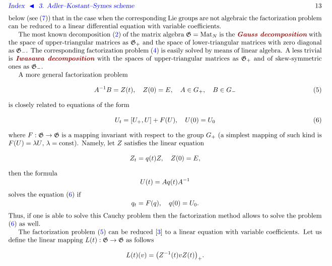
below (see (7)) that in the case when the corresponding Lie groups are not algebraic the factorization problemcan be reduced to a linear differential equation with variable coefficients.

The most known decomposition (2) of the matrix algebra G = MatN is the Gauss decomposition withthe space of upper-triangular matrices as G+ and the space of lower-triangular matrices with zero diagonalas G−. The corresponding factorization problem (4) is easily solved by means of linear algebra. A less trivialis Iwasawa decomposition with the spaces of upper-triangular matrices as G+ and of skew-symmetricones as G−.

A more general factorization problem

A−1B = Z(t), Z(0) = E, A ∈ G+, B ∈ G− (5)

is closely related to equations of the form

Ut = [U+, U ] + F (U), U(0) = U0 (6)

where F : G→ G is a mapping invariant with respect to the group G+ (a simplest mapping of such kind isF (U) = λU , λ = const). Namely, let Z satisfies the linear equation

Zt = q(t)Z, Z(0) = E,

then the formula

U(t) = Aq(t)A−1

solves the equation (6) if

qt = F (q), q(0) = U0.

Thus, if one is able to solve this Cauchy problem then the factorization method allows to solve the problem(6) as well.

The factorization problem (5) can be reduced [3] to a linear equation with variable coefficients. Let usdefine the linear mapping L(t) : G→ G as follows

L(t)(v) =(Z−1(t)vZ(t)

)+.

Index J 3. Adler–Kostant–Symes scheme 14

Since L(0) is the identity map, hence L(t) is invertible for small t. Let A be the solution of Cauchy problem

At = −AL−1(t)((Z−1Zt)+

), A(0) = E, (7)

then the pair A, B = AZ(t) is the unique solution of the factorization problem (5).

2. Reductions and nonassociative algebras

It is clear from (3) that if the initial data U0 belong to a vector space M which is G+-module then U(t) ∈Mfor all t. We call such a specialization of the (1) as M-reduction. The possibility of reductions greatlyextends the frames of the factorization method (see e.g. [4]).

There are deep relations between M -reductions and several classes of nonassociative algebras [5, 4]. LetR : M → G+ denote the projector onto G+ parallel to G−. It terms of the operator R, the M -reduction iswritten as

mt = [R(m),m], m ∈M. (8)

Let us consider the algebraic operation on M defined by formula

m ∗ n = [R(m), n]. (9)

The system (8) takes, in terms of this multiplication, the form

mt = m ∗m. (10)

Let us show that if the multiplication ∗ is left-symmetric then the system (10) is integrable by factorizationmethod. Let A be a left-symmetric algebra. Let G = A ⊕ A. Since the operation [X,Y ] = X ∗ Y − Y ∗Xdefines a Lie algebra for any left-symmetric algebra A, hence the vector space G becomes the Lie algebrawith respect to the bracket [

(g1, a1), (g2, a2)]

=([g1, g2], g1 ∗ a2 − g2 ∗ a1

).

It is clear from this formula that G+ = (q, 0) and G− = (q,−q) are subalgebras in G. The equation (1)for U = (p, q) corresponding to the decomposition G = G+ ⊕G− is of the form

pt = q ∗ p− p ∗ q, qt = p ∗ q + q ∗ q.

Index J 3. Adler–Kostant–Symes scheme 15

In order to obtain the A-top (10) as a M -reduction of this system it is sufficient to set p = 0, that is, tochoose M = (0, q).

It should be noted that the operation (9) is left-symmetric if and only if the operator R : M → G+

satisfies the relation (cf [6])

R([R(a), b] + [a,R(b)])− [R(a), R(b)] ∈ Ann(M)

where a, b are any elements of M and Ann(M) denotes the set of G+ elements with zero image of M .

References

[1] M. Adler. On a trace functional for formal pseudo-differential operators and the symplectic structure of theKorteweg-de Vries type equations. Invent. math. 50 (1979) 219–248.

[2] B. Kostant. Quantization and representation theory. Lect. Notes 34 (1979) 287–316.

[3] I.Z. Golubchik, V.V. Sokolov. On some generalizations of the factorization method. Theor. Math. Phys. 110:3(1997) 267–276.

[4] I.Z. Golubchik, V.V. Sokolov. Generalized operator Yang–Baxter equations, integrable ODEs and nonassociativealgebras. J. Nonl. Math. Phys. 7:2 (2000) 184–197.

[5] I.Z. Golubchik, V.V. Sokolov, S.I. Svinolupov. A new class of nonassociative algebras and a generalized factor-ization method. Preprint ESI 53, Wien, 1993.

[6] M.A. Semenov-Tyan-Shansky. What a classical r-matrix is. Funct. Anal. Appl. 17:4 (1983) 17–33.

Index J 4. Algebraic structures 16

4 Algebraic structures

The set G equipped with the multiplication G×G→ G is called group if the following identities are fulfilled:

associativity ∀ a, b, c a(bc) = a(bc),

unit element ∃ e : ∀ a ea = ae = a,

inverse element ∀ a ∃ a−1 : a(bc) = a(bc).

(1)

An algebra is a vector space A over a field F , equipped with a multiplication A × A → A which satisfiesthe identities

(αa+ βb)c = αac+ βbc, c(αa+ βb) = αca+ βcb, ∀ a, b, c ∈ A, ∀ α, β ∈ F.

The important classes of algebras are characterized by some additional identities, for example:

commutative algebra ab = ba

anticommutative algebra ab = −baassociative algebra a(bc) = (ab)c

Lie algebra ab = −ba, a(bc) + b(ca) + c(ab) = 0

Jordan algebra ab = ba, (ab)a2 = a(ba2)

left-symmetric algebra a(bc)− (ab)c = b(ac)− (ba)c

An important example of an algebraic structure with ternary multiplication is given by Jordan pairs.

A linear mapping F : A→ A is called a differentiation of an algebra A if it satisfies the Leibniz rule

F (ab) = F (a)b+ aF (b).

The set of all differentiations of the algebra is denoted Der(A). It is a Lie algebra itself with respect to thecommutator [F,G](a) = F (G(a))−G(F (a)). Indeed,

[F,G](ab) = F (G(a)b+ aG(b))−G(F (a)b+ aF (b))

Index J 4. Algebraic structures 17

= F (G(a))b+G(a)F (b) + F (a)G(b) + aF (G(b))−G(F (a))b− F (a)G(b)−G(a)F (b)− aG(F (b))

= [F,G](a)b+ a[F,G](b),

and it is easy to check that the Jacobi identity is fulfilled.

Index J 5. Backlund transformation 18

5 Backlund transformation

Backlund transformation between equations F [u] = 0, G[u] = 0 is a set of relations A[u, u] = 0, B[u, u] =0 which satisfy the property that elimination of u yields the given equation for u and vice versa. The mostimportant is the case when the equations coincide (or differ in the values of parameters). In this case theterm Backlund autotransformation is used. Iterations of auto-BT generate the differential-differenceequations, or lattices.

ã The simplest example is given by the Cauchy–Riemann equations ux = vy, uy = −vx; here both u andv satisfy the Laplace equation uxx + uyy = 0.

ã The first nontrivial nonlinear example was introduced by L. Bianchi and A.V. Backlund in the 1880’s.Geometrically, it describes a transformation of pseudospherical surfaces. Analytically, it can be brought tothe pair of relations

ux + ux = a sin(u− u), uy − uy =1

2asin(u+ u) (1)

and one can easily check that both u and u satisfy, in virtue of these relations, the sine-Gordon equation

uxy = sin 2u.

Let u = un and u = un+1, then the x-part of this auto-BT gives rise to the lattice

un+1,x + un,x = an sin(un+1 − un)

which is an example of the so-called dressing chains.

ã In all known examples, the construction of BT is somehow related with the auxiliary linear problemsassociated with the equation under consideration. The most important BT are Darboux transformationswhich make use of a particular solution of the linear problems. On the nonlinear level such transformation isusually given by Riccati-type equations, like in (1). Another type of BT is given by explicit transformationslike the invertible substitution

u = ux/u+ v, v = u

which acts on the solutions of the Levi system

ut = uxx + (u2 + 2uv)x, vt = −vxx + (v2 + 2uv)x.

Index J 5. Backlund transformation 19

This substitution generates (again, let u = un and u = un+1) the Volterra lattice

un,x = un(un+1 − un−1).

ã The term Backlund transformation is also widely used in the theory of Painleve-type ODE. In thiscontext it denotes a rational differential substitution between equations with different parameter sets. Forexample, the second Painleve equation

u′′ = 2u3 + zu+ a

admits the pair of BT

u = u± 2a± 1

2u′ ± 2u2 ± z, a = ±1− a

which allows to generate solutions for all values of the parameter a+ 2n, −a+ 2n+ 1, n ∈ Z.

References

[1] A.V. Backlund. Zur Theorie der Flachentransformationen. Math. Ann. 19:3 (1881) 387–422.

[2] L. Bianchi. Sulla trasformazione di Backlund per le superficie pseudosferiche. Rend. Ac. Naz. dei Lincei 5 (1892)3–12.

[3] R.M. Miura (ed). Backlund transformations, the Inverse Scattering Method, solitons, and their applications.NSF Research Workshop on Contact Transformations (Nashville, Tennessee 1974). Lect. Notes in Math. 515,Springer-Verlag, 1976.

[4] R. Hermann. The geometry of nonlinear differential equations, Backlund transformations, and solitons. Math.Sci. Press, Brookline, 1977.

[5] G.L. Lamb, jr. Elements of soliton theory. New York: J. Wiley, 1980.

[6] M.J. Ablowitz, H. Segur. Solitons and the Inverse Scattering Transform. Philadelphia: SIAM, 1981.

[7] C. Rogers, W.F. Shadwick. Backlund transformations and their applications. New York: Academic Press, 1982.

[8] F. Calogero, A. Degasperis. Spectral transform and solitons: tools to solve and investigate nonlinear evolutionequations, I. Amsterdam: North-Holland, 1982.

[9] V. Matveev, M. Salle. Darboux transformations and solitons. Springer-Verlag, 1991.

Index J 5. Backlund transformation 20

[10] C. Rogers, W.K. Schief. Backlund and Darboux transformations. Geometry and modern applications in solitontheory. Cambridge University Press, Cambridge, 2002.

[11] C. Gu, H. Hu, Z. Zhou. Darboux transformations in integrable systems theory and their applications to geometry.Math. Phys. Studies 25, Springer, 2005.

Index J 6. Bakirov system eDD 21

6 Bakirov system

ut = 5u4 + v2, vt = v4

The only higher symmetry of this system is

ut = 11u6 + 5vv2 + 4v21 , vt = v6.

Bakirov checked that there are no other symmetries up to order 53. The rigorous proof was obtained in [2].

ã See also: Fokas conjecture.

References

[1] I.M. Bakirov. On the symmetries of some system of evolution equations. Preprint Inst. of Math., Ufa, 1991. (inRussian)

[2] F. Beukers, J.A. Sanders, J.P. Wang. One symmetry does not imply integrability. J. Diff. Eq. 146:1 (1998)251–260.

Index J 7. Belousov–Zhabotinsky model D 22

7 Belousov–Zhabotinsky model

u = av(1− u) + au(1− bu), v = −1

av(1 + u) + cw, w = d(u− w)

References

[1] A.M. Zhabotinskii. Periodic course of oxidation of malonic acid in solution (investigation of the kinetics of thereaction of Belousov). Biophysics 9 (1964) 329–335.

[2] A.M. Zhabotinskii, A.N. Zaikin, M.D. Korzukhin, G.P. Kreitser. Mathematical model of a self-oscillating chem-ical reaction (oxidation of bromomalonic acid with bromate catalyzed by cerium ions). Kinetics and Catalysis12 (1971) 516–521.

Index J 8. Belov–Chaltikian lattices eD∆ 23

8 Belov–Chaltikian lattices

u(j)n,x = u(j)

n (u(1)n+j − u

(1)n−1) + u(j+1)

n − u(j+1)n−1 , j = 1, . . . ,M, u(M+1)

n = 0.

References

[1] A.A. Belov, K.D. Chaltikian. Lattice analogues of W -algebras and classical integrable equations. Phys. Lett. B309 (1993) 268–274.

[2] A.A. Belov, K.D. Chaltikian. Lattice analogue of the W∞ algebra and discrete KP hierarchy. Phys. Lett. B 317(1993) 64–72.

[3] Yu.B. Suris. The problem of integrable discretization: Hamiltonian approach. Basel: Birkhauser, 2003.

Index J 9. Benjamin–Bona–Mahoney–Peregrine equation DD 24

9 Benjamin–Bona–Mahoney–Peregrine equation

ut + ux − uxxt + uux = 0

Alias: regularized long wave equation

ã As the famous KdV equation, this one describes one-dimensional long waves of small amplitude [1].

ã Some (nonintegrable) generalizations in any dimension were studied in [5].

References

[1] T.B. Benjamin, J.L. Bona, J.J. Mahoney. Model equations for long waves in nonlinear dispersive systems. Phil.Trans. R. Soc. Lond. Ser. A 272:1220 (1972) 47–78.

[2] H. Peregrine. J. Fluid Mech. 25 (1966) 321–330.

[3] P.J. Olver. Euler operators and conservation laws of the BBM equation. Math. Proc. Camb. Phil. Soc. 85 (1979)143–160.

[4] J.B. McLeod, P.J. Olver. The connection between partial differential equations soluble by inverse scattering andordinary differential equations of Painleve type. SIAM J. Math. Anal. 14 (1983) 488–506.

[5] J. Avrin, J.A. Goldstein. Global existence for the Benjamin–Bona–Mahony equation in arbitrary dimensions.Nonlinear Anal. 9:8 (1985) 861–865

Index J 10. Benjamin–Ono equation eDD 25

10 Benjamin–Ono equation

ut +H(uxx)− 6uux = 0, H(f) =1

πv.p.

∫ ∞−∞

f(y)

y − xdy

Operator H is called the Hilbert transform.The equation describes one-dimensional waves in deep water.

References

[1] T.B. Benjamin. Internal waves of permanent form in fluids of great depth. J. Fluid Mech. 29 (1967) 559–562.

[2] F. Calogero, A. Degasperis. Spectral transform and solitons: tools to solve and investigate nonlinear evolutionequations, I. Amsterdam: North-Holland, 1982.

[3] A.S. Fokas, B. Fuchssteiner. The hierarchy of the Benjamin–Ono equation. Phys. Lett. A 86:6–7 (1981) 341–345.

[4] H. Ono. Algebraic solitary waves in stratified fluids. J. Phys. Soc. Japan 39 (1975) 1082–1091.

Index J 11. Benney chain dD∆ 26

11 Benney chain

un,t = un+1,x + nun−1u0,x, n = 0, 1, 2, . . .

ã Dispersionless Lax pair Dt(L) = ApLx −AxLp:

A =p2

2+ u0, L = p+ u0p

−1 + u1p−2 + u2p

−3 + . . .

References

[1] D.J. Benney. Some properties of long nonlinear waves. Stud. Appl. Math. 52 (1973) 45–50.

[2] J. Gibbons. Collisionless Boltzmann equations and integrable moment equations. Physica D 3 (1981) 503–511.

[3] B.A. Kupershmidt, Yu.I. Manin. Long wave equation with free boundaries. I. Conservation laws. Funct. Anal.Appl. 11:3 (1977) 188–197.

[4] B.A. Kupershmidt, Yu.I. Manin. Long wave equations with a free surface. II. The Hamiltonian structure andthe higher equations. Funct. Anal. Appl. 12:1 (1978) 25–37.

[5] D.R. Lebedev. Benney’s long wave equations: Hamiltonian formalism. Lett. Math. Phys. 3 (1979) 481–488.

[6] D.R. Lebedev, Yu.I. Manin. Conservation laws and representation of Benney’s long wave equations. Phys. Lett.A 74:3,4 (1979) 154–156.

[7] V.E. Zakharov. Benney’s equations and quasi-classical approximation in the inverse problem method. Funct.Anal. Appl. 14:2 (1980) 89–98.

Index J 12. Benney equation dDD 27

12 Benney equation

ut + uux − uy∫ y

0

uxdy + hx = 0, ht +Dx

(∫ h

0

udy)

= 0

References

[1] V.E. Zakharov. On the Benney’s equations. Physica D 3 (1981) 193–200.

Index J 13. Bogoyavlensky–Narita lattices eD∆ 28

13 Bogoyavlensky–Narita lattices

un,xk= un

k∑s=1

(un+s − un−s) (1)

ã Introduced in [1, 2].

ã The flow corresponding to xk does not commute with the rest flows of the family, rather it serves as thesimplest member of an integrable hierarchy on its own. The next order flows and associated systems are (nis omitted):

ux1= u(u1 − u−1)

ut1 = u(u1(u2 + u1 + u)− u−1(u+ u−1 + u−2))→

u1,t1 = Dx1

(u1,x1+ u1(u1 + 2u0))

u0,t1 = Dx1(−u0,x1

+ (2u1 + u0)u0)

(this is Volterra lattice and Levi system);

ux2 = u(u2 + u1 − u−1 − u−2)

ut2 = u(u2(u4 + · · ·+ u) + u1(u3 + · · ·+ u)

− u−1(u+ · · ·+ u−3)− u−2(u+ · · ·+ u−4))

→

u3,t2 = Dx2(u3,x2 + u3(u3 + 2u2 + 2u1))

u2,t2 = Dx2(u2,x2 + u2(u2 + 2u1 + 2u0))

u1,t2 = Dx2(−u1,x2 + (2u3 + 2u2 + u1)u1)

u0,t2 = Dx2(−u0,x2 + (2u2 + 2u1 + u0)u0);

ux3

= u(u3 + u2 + u1 − u−1 − u−2 − u−3)

ut3 = u(u3(u6 + · · ·+ u) + u2(u5 + · · ·+ u)

+ u1(u4 + · · ·+ u)− u−1(u+ · · ·+ u−4)

− u−2(u+ · · ·+ u−5)− u−3(u+ · · ·+ u−6))

→

u5,t3 = Dx3(u5,x3 + u5(u5 + 2u4 + 2u3 + 2u2))

u4,t3 = Dx3(u4,x3 + u4(u4 + 2u3 + 2u2 + 2u1))

u3,t3 = Dx3(u3,x3 + u3(u3 + 2u2 + 2u1 + 2u0))

u2,t3 = Dx3(−u2,x3 + (2u5 + 2u4 + 2u3 + u2)u2)

u1,t3 = Dx3(−u1,x3 + (2u4 + 2u3 + 2u2 + u1)u1)

u0,t3 = Dx3(−u0,x3 + (2u3 + 2u2 + 2u1 + u0)u0)

and so on.

Index J 13. Bogoyavlensky–Narita lattices eD∆ 29

ã Bogoyavlensky lattices admit a lot of modifications. Some of the difference substitutions for this type oflattices can be described as follows. Let a lattice be given

un,x = unf(un), f = a(k)T k + · · ·+ a(−k)T−k, (2)

where f is a Laurent polynomial on the shift operator T : un → un+1. This polynomial can be factored inmany ways into the product of two Laurent polynomials and any such factorization generates the substitutionfrom (1) to the lattice (2)

vn,x = vnh(eg(log vn))un = eg(log vn)

−−−−−−−−−−−→ un,x = unf(un), f = gh.

It is easy to see that the lattice for the variables vn is polynomial if and only if all coefficients of thepolynomial g are nonnegative integers, moreover, the total degree of its r.h.s. is equal to the sum of thecoefficients of g plus 1.

Notice that the polynomial f for the Bogoyavlensky lattice (1) is

f = T k + · · ·+ T − T−1 − · · · − T−k =(T k − 1)(T k+1 − 1)

(T − 1)T k.

Example 1. Consider the lattice

un,x = un(un+2 + un+1 − un−1 − un−2),

corresponding to the polynomial f = T 2+T−T−1−T−2. Several possible choices of g and the correspondingsubstitutions are:

g = T + 1 un = vn+1vn vn,x = vn(vn+2vn+1 − vn−1vn−2);

g = T 2 + T + 1 un = vn+2vn+1vn vn,x = v2n(vn+2vn+1 − vn−1vn−2);

g = T 3 − 1 un = vn+3/vn vn,x = vn(vn+2/vn−1 + vn+1/vn−2).

Index J 13. Bogoyavlensky–Narita lattices eD∆ 30

References

[1] K. Narita. Soliton solution to extended Volterra equation. J. Phys. Soc. Japan 51:5 (1982) 1682–1685.

[2] O.I. Bogoyavlensky. Algebraic constructions of integrable dynamical systems — extensions of the Volterra sys-tem. Russ. Math. Surveys 46:3 (1991) 1–64.

[3] O.I. Bogoyavlensky. Breaking solitons. Nonlinear integrable equations. Moscow: Nauka, 1991.

[4] Y. Itoh. Integrals of a Lotka–Volterra system of odd number of variables. Progr. Theor. Phys. 78 (1987) 507–510.

Index J 14. Boltzman equation eDD 31

14 Boltzman equation

ut = uu2 + u21

The equation is not integrable. The first necessary condition (23.2), (23.3) is not fulfilled:

ρ−1 = u−1/2, Dt(ρ−1) 6∈ ImDx.

References

[1] L. Dresner. Similarity solutions of nonlinear partial differential equations. Res. Notes in Math. 88, Boston:Pitman, 1983.

Index J 15. Born–Infeld equation hDD 32

15 Born–Infeld equation

(1− u2t )uxx + 2uxutuxt − (1 + u2

x)utt = 0

ã Lagrangian: L = (1− u2t + u2

x)1/2.

ã See also: the minimal surfaces equation

References

[1] M. Born, L. Infeld. Foundations of a new field theory. Proc. Roy. Soc. A 144 (1934) 425–451.

[2] R. Courant. Partial differential equations, 1962.

[3] G.B. Whitham. Linear and nonlinear waves, N.Y.: Wiley, 1974.

Index J 16. Boussinesq equation eDD 33

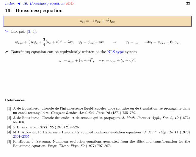
16 Boussinesq equation

utt = −(uxx + u2)xx

ã Lax pair [3, 4]:

ψxxx +3

2uψx +

3

4(ux + v)ψ = λψ, ψt = ψxx + uψ ⇒ ut = vx, −3vt = uxxx + 6uux.

ã Boussinesq equation can be equivalently written as the NLS type system

ut = uxx + (u+ v)2, −vt = vxx + (u+ v)2.

References

[1] J. de Boussinesq. Theorie de l’intumescence liquid appelee onde solitaire ou de translation, se propagente dansun canal rectangulaire. Comptes Rendus Acad. Sci. Paris 72 (1871) 755–759.

[2] J. de Boussinesq. Theorie des ondes et de remous qui se propagent. J. Math. Pures et Appl., Ser. 2, 17 (1872)55–108.

[3] V.E. Zakharov. JETP 65 (1973) 219–225.

[4] M.J. Ablowitz, R. Haberman. Resonantly coupled nonlinear evolution equations. J. Math. Phys. 16:11 (1975)2301–2305.

[5] R. Hirota, J. Satsuma. Nonlinear evolution equations generated from the Backlund transformation for theBoussinesq equation. Progr. Theor. Phys. 57 (1977) 797–807.

Index J 17. Boussinesq system, twodimensional eDDD 34

17 Boussinesq system, twodimensional

ut = uxx + 2vx, −vt = vxx − 2uux + 2uy

Elimination of v yields the equation

utt = (uxxx + 4uux − 4uy)x

which coincides with Kadomtsev–Petviashvili equation up to the scaling and exchange y ↔ t.

Index J 18. Box-ball system CA 35

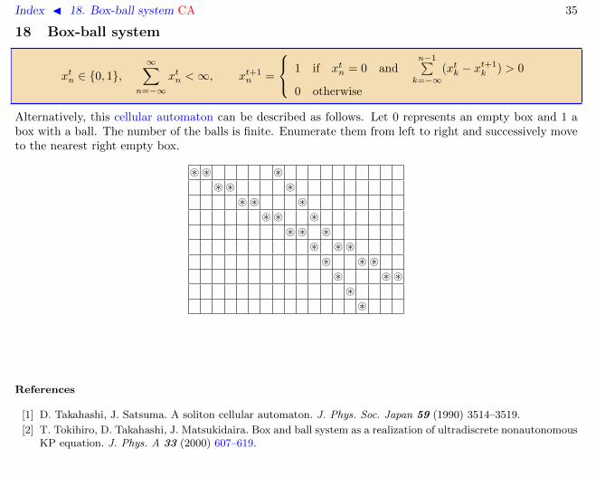
18 Box-ball system

xtn ∈ 0, 1,∞∑

n=−∞xtn <∞, xt+1

n =

1 if xtn = 0 andn−1∑k=−∞

(xtk − xt+1k ) > 0

0 otherwise

Alternatively, this cellular automaton can be described as follows. Let 0 represents an empty box and 1 abox with a ball. The number of the balls is finite. Enumerate them from left to right and successively moveto the nearest right empty box.

~~ ~~~ ~~~ ~

~~ ~~~ ~~ ~~~ ~~~ ~~~~

References

[1] D. Takahashi, J. Satsuma. A soliton cellular automaton. J. Phys. Soc. Japan 59 (1990) 3514–3519.

[2] T. Tokihiro, D. Takahashi, J. Matsukidaira. Box and ball system as a realization of ultradiscrete nonautonomousKP equation. J. Phys. A 33 (2000) 607–619.

Index J 19. Boyer–Finley equation dDDD 36

19 Boyer–Finley equation

uxx + uyy = eututt

References

[1] C.P. Boyer, J.D. Finley. Killing vectors in self-dual Euclidean Einstein spaces. J. Math. Phys. 23 (1982) 1126–1130.

Index J 20. Burgers equation eDD 37

20 Burgers equation

ut = uxx + 2uux

ã This equation is probably the simplest nonlinear model with applications in hydrodynamics, gas dynamicsand acoustic.

ã The potential Burgers hierarchy (u = v1) can be defined explicitly by formula

vtn = (Dx + v1)n(1) = Yn(v1, . . . , vn), vk = Dkx(v)

where Yn are Bell polynomials. The following formula for their generating function is easily proven bydifferentiation with respect to z and x:

1 +

∞∑n=1

Ynzn

n!= exp

( ∞∑n=1

vnzn

n!

)= ev(x+z)−v(x).

ã The Cole–Hopf transformation [2, 3]

v = log φ ⇒ u = φx/φ

linearizes the whole hierarchy:

1 +

∞∑n=1

Ynzn

n!=φ(x+ z)

φ(x)= 1 +

∞∑n=1

φnφ

zn

n!.

References

[1] J.M. Burgers. A mathematical model illustrating the theory of turbulence. Adv. Appl. Mech. 1 (1948) 171–199.

[2] J.D. Cole. On a quasilinear parabolic equation occuring in aerodynamics. Q. Appl. Math. 9 (1950) 225–236.

[3] E. Hopf. The partial differential equation ut = uux + µuxx. Comm. Pure and Appl. Math. 3 (1950) 201–230.

Index J 21. Burgers–Huxley equation eDD 38

21 Burgers–Huxley equation

ut = uxx + uux + u(u− 1)(u− a)

Not integrable.

ã See also: Fischer, Kolmogorov–Petrovsky–Piskunov equations.

References

[1] J. Satsuma. Explicit solutions of nonlinear equations with density dependent diffusion. J. Phys. Soc. Japan 56(1987) 1947–1950.

[2] J. Satsuma. Exact solutions of Burgers equation with reaction terms. pp. 255–262 in Topics in soliton theoryand exactly solvable nonlinear equations. (M.J. Ablowitz, B. Fuchssteiner, M.D. Kruskal eds). Singapore: WorldScientific, 1987.

Index J 22. Burgers–Korteweg–de Vries equation eDD 39

22 Burgers–Korteweg–de Vries equation

ut = auxxx + buxx + uux

This equation serves as the simplest model for one-dimensional nonlinear waves in the media with dispersionand dissipation. It has some applications in plasma physics for the description of collisionless shock waves.In contrast to both Burgers equation (a = 0) and KdV equation (b = 0) this one is not integrable.

References

[1] R.Z. Sagdeev. J. Theor. Phys. 31 (1961) 1955.

[2] J. Canosa, J. Gazdag. The Korteweg–de Vries–Burgers Equation. J. Comput. Phys. 23 (1977) 393–403.

[3] G.M. Zaslavsky, R.Z. Sagdeev. Introduction to nonlinear physics. Moscow, Nauka, 1988.

Index J 23. Burgers-type equations, the classification eDD 40

23 Burgers-type equations, the classification

Author: V.E. Adler, 29.03.2007

1. The necessary integrability conditions2. The analysis of the first necessary condition3. The conclusion of the proof

Burgers type equations are integrable evolutionary equations of the second order

ut = F (u2, u1, u, x), un = Dnx (u). (1)

Here we present their exhaustive classification obtained by Svinolupov. The proof of the following theoremcan be converted into a test of integrability applicable to a given equation of the form (1). Moreover, if theequation turns out to be integrable then the change of variables can be found constructively which relatesit to one of the equations from the list.

Theorem 1 (Svinolupov [1]). If equation (1) possesses a higher symmetry of order ≥ 3 then it possesses aninfinite algebra of higher symmetries and is contact equivalent to one of the following equations, linearizablevia differential substitutions (f denotes an arbitrary function):

ut = u2 + f(x)u, (B1)

ut = Dx(u1 + u2 + f(x)), (B2)

ut = Dx

(u1

u2− 2x

), (B3)

ut = Dx

(u1

u2+ ε1xu+ ε2u

). (B4)

1. The necessary integrability conditions

Accordingly to the general theory (see formal symmetry test), the necessary integrability conditions are ofthe form of the conservation laws

Dx(σk) = Dt(ρk), k = −1, 0, 1, . . . (2)

Index J 23. Burgers-type equations, the classification eDD 41

where the densities ρk are algorithmically expressed through the right hand side of the equation and thepreviously defined σi. For the equations (1) we will need only first three conditions.

Lemma 2. If the equation (1) possesses a higher symmetry of order ≥ 3 then the equations (2) at k = −1, 0, 1are fulfilled with

ρ−1 = F−1/2u2

, ρ0 = Fu1F−1u2− σ−1F

−1/2u2

,

ρ1 =1

8(4Fu + 2σ0 + σ2

−1)F−1/2u2

− 1

32(2Fu1

−Dx(Fu2))2F−3/2

u2.

(3)

2. The analysis of the first necessary condition

In the case of equations (1), the analysis of the integrability conditions is simplified due to the followinglemma.

Lemma 3. The order of a conservation law of the equation (1) is equal to 0 or 2.

Proof. The conservation law satisfies the equation

(Dt + F ᵀ∗ )( δρδu

)= 0

whereδρ

δu= ρu −Dx(ρu1) +D2

x(ρu2)− · · ·+ (−Dx)m(ρum) = a(x, u, . . . , um)u2m + . . . .

Collecting the terms with u2m+2 yields

aD2mx (F ) +D2

x(aFu2u2m) + · · · = 0 (4)

and if 2m > 2 then 2aFu2u2m+2 = 0, hence a = 0.

Moreover, the order of the conservation law determines the dependence of F on u2. Indeed, if the equationpossesses a conservation law of order 2, then, accordingly to (4),

2Fu2+ u2Fu2u2

= 0 ⇔ F = (fu2 + g)−1 + h (5)

Index J 23. Burgers-type equations, the classification eDD 42

where f, g, h depend on x, u, u1. If the order of a conservation law is 0 then equation is quasilinear: letρ = ρ(x, u), ρu 6= 0, then

Dt(ρ) = ρuF ∈ ImDx ⇒ F = f(x, u, u1)u2 + g(x, u, u1). (6)

The equation with another dependence of the right hand side on u2 cannot possess the nontrivial conservationlaw at all.

Now let us consider the first integrability condition Dt(F−1/2u2 ) ∈ ImDx. The quantity F

−1/2u2 is called

the separant of the equation. Accordingly to the Lemma 3 it must be linear in u2. Three cases are possible:

1) F−1/2u2

= Dx(α(x, u, u1)),

2) F−1/2u2

= Dx(α(x, u, u1)) + β(x, u), βu 6= 0,

3) F−1/2u2

= Dx(α(x, u, u1)) + β(x, u, u1), βu1u16= 0.

In the case 1) the conservation law is trivial, and in the cases 2), 3) its order is equal, respectively, to 0 and2. The functions α and β are not independent. Since β is the density of the conservation law, hence

Dt(β(x, u, u1)) ∼ (βu −Dx(βu1))F ∈ ImDx ⇒ ∂2u2

((βu −Dx(βu1))F ) = 0.

The last equation is equivalent to

βu1u1(αx + αuu1 + β) = αu1

(βu1x − βu + βu1uu1). (7)

In particular, the function α does not depend on u1 in the case 2), while αu1 6= 0 in the case 3). This is alsoclear from the formulae (6), (5).

Lemma 4. The equation (1) satisfies the condition Dt(F−1/2u2 ) ∈ ImDx if and only if it is contact equivalent

to one of the quasi-linear equations

ut = u2 + f(x, u, u1), (8)

ut = Dx

(u1

u2+ f(x, u)

). (9)

Index J 23. Burgers-type equations, the classification eDD 43

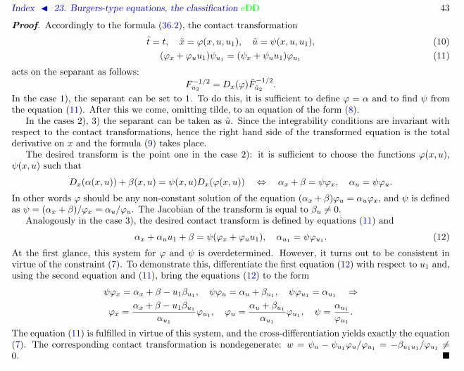
Proof. Accordingly to the formula (36.2), the contact transformation

t = t, x = ϕ(x, u, u1), u = ψ(x, u, u1), (10)

(ϕx + ϕuu1)ψu1= (ψx + ψuu1)ϕu1

(11)

acts on the separant as follows:

F−1/2u2

= Dx(ϕ)F−1/2u2

.

In the case 1), the separant can be set to 1. To do this, it is sufficient to define ϕ = α and to find ψ fromthe equation (11). After this we come, omitting tilde, to an equation of the form (8).

In the cases 2), 3) the separant can be taken as u. Since the integrability conditions are invariant withrespect to the contact transformations, hence the right hand side of the transformed equation is the totalderivative on x and the formula (9) takes place.

The desired transform is the point one in the case 2): it is sufficient to choose the functions ϕ(x, u),ψ(x, u) such that

Dx(α(x, u)) + β(x, u) = ψ(x, u)Dx(ϕ(x, u)) ⇔ αx + β = ψϕx, αu = ψϕu.

In other words ϕ should be any non-constant solution of the equation (αx + β)ϕu = αuϕx, and ψ is definedas ψ = (αx + β)/ϕx = αu/ϕu. The Jacobian of the transform is equal to βu 6= 0.

Analogously in the case 3), the desired contact transform is defined by equations (11) and

αx + αuu1 + β = ψ(ϕx + ϕuu1), αu1 = ψϕu1 . (12)

At the first glance, this system for ϕ and ψ is overdetermined. However, it turns out to be consistent invirtue of the constraint (7). To demonstrate this, differentiate the first equation (12) with respect to u1 and,using the second equation and (11), bring the equations (12) to the form

ψϕx = αx + β − u1βu1 , ψϕu = αu + βu1 , ψϕu1 = αu1 ⇒

ϕx =αx + β − u1βu1

αu1

ϕu1, ϕu =

αu + βu1

αu1

ϕu1, ψ =

αu1

ϕu1

.

The equation (11) is fulfilled in virtue of this system, and the cross-differentiation yields exactly the equation(7). The corresponding contact transformation is nondegenerate: w = ψu − ψu1

ϕu/ϕu1= −βu1u1

/ϕu16=

0.

Index J 23. Burgers-type equations, the classification eDD 44

3. The conclusion of the proof

The Lemma 4 resolves effectively the first integrability condition and reduces the general problem to thequasilinear one. The further analysis is relatively easy. We perform it separately for the cases (8) and (9).

Proof of Theorem 1. 1) Consider equations of the form (8) first. The canonical densities take the form

ρ0 = fu1, ρ1 ∼

1

2fu +

1

4σ0.

Since the quasilinear equation can possess only zero order conservation laws, hence the density ρ0 must belinear in u1, so that the equation is of the form

ut = u2 + a(x, u)u21 + b(x, u)u1 + c(x, u).

This subclass is invariant with respect to the changes x = x, u = ψ(x, u), and the coefficient a is transformedaccordingly to the formula ψ2

ua(x, ψ) = ψua(x, u)−ψuu. Therefore, the equation can be brought to the form

ut = u2 + b(x, u)u1 + c(x, u).

Consider the condition Dt(b) ∈ ImDx:

Dt(b) = bu(u2 + bu1 + c) = Dx

(buu1 +

1

2b2)− u1Dx(bu)− bbx + buc ∈ ImDx.

It is easy to see that it is equivalent to

b = p(x)u+ q(x), up′′ − (pu+ q)(p′u+ q′) + pc ∈ ImDx.

Notice, that we may still use the changes

u = µ(x)u+ ν(x) ⇒ p = µp, q = 2µ′/µ+ νp+ q.

Therefore, the function p can be made constant, and q can be set to zero. After this, if p 6= 0, then c = c(x)and we obtain the equation (B2). If p = 0 then the function c is determined by the third integrabilitycondition. In this case fu = cu must be the density of the conservation law, that is

Dt(cu) = cuu(u2 + c) ∈ ImD ⇔ D2x(cuu) + cuuu(u2 + c) + cuucu = 0 ⇔ cuu = 0.

Index J 23. Burgers-type equations, the classification eDD 45

The change u = u+ ν(x) brings to the equation (B1).2) Now, consider the equations of the form (9). In this case the second integrability condition takes the

formDt(u

2fu − uf) ∈ ImDx. (13)

We have, for the density of the form ρ = ρ(x, u),

Dt(ρ) = ρuDx(u−2u1 + f) ∼ −Dx(ρu)(u−2u1 + f) ∈ ImDx ⇒ ρuu = 0,

and thereforef = p(x)u+ q(x) + r(x)/u.

The transformx = ϕ(x), u = u/ϕ′(x)

does not change the form of the equation and maps the coefficient f into f = f + ϕ′′/(ϕ′u). Use of thistransform allows to set r = 0, without loss of generality. To do this, it is sufficient to define ϕ as a nonconstantsolution of the equation ϕ′′ = −rϕ′. Then the condition (13) is reduced to the following one:

−Dt(qu) ∼ q′(u−2u1 + pu) ∼ q′′u−1 + q′pu ∈ ImDx ⇒ q′′ = q′p = 0.

If q′ 6= 0 then p = 0 and the scaling x = kx, u = u/k brings to the equation (B3).If q′ = 0 then p should be specified by use of the third integrability condition. In this subcase it takes

the form 4ρ1 = 18u−3u21 − 9u−2u2 − 3p′u− pu1 ∼ −2p′u. Therefore,

−Dt(p′u) ∼ p′′(u−2u1 + pu) ∼ p′′′u−1 + p′′pu ∈ ImDx ⇒ p′′ = 0,

and this corresponds to equation (B4).

References

[1] S.I. Svinolupov. Second-order evolution equations with symmetries. Russ. Math. Surveys 40:5 (1985) 241–242.

Index J 24. Calogero equation hDD 46

24 Calogero equation

uxt = uuxx + Φ(ux)

Liouville type equation.

ã Particular case: Hunter–Saxton equation [3, 4]

uxt = uuxx + εu2x

References

[1] F. Calogero. A solvable nonlinear wave equation. Stud. Appl. Math. 70:3 (1984) 189–199.

[2] M.V. Pavlov. The Calogero equation and Liouville type equations. nlin.SI/0101034

[3] J.K. Hunter, R. Saxton. Dynamics of director fields. SIAM J. on Appl. Math. 51:6 (1991) 1498–1521.

[4] P.J. Olver, P. Rosenau. Tri-Hamiltonian duality between solitons and solitary wave solutions having compactsupport. Phys. Rev. E 53:2 (1996) 1900–1906.

Index J 25. Calogero–Degasperis equation, elliptic eDD 47

25 Calogero–Degasperis equation, elliptic

ut = u3 −3u1u

22

2(u21 + 1)

− 3

2℘(u)u1(u2

1 + 1)− 2au1, ℘2 = 4℘3 + g1℘+ g2

Index J 26. Calogero–Degasperis equation, exponential eDD 48

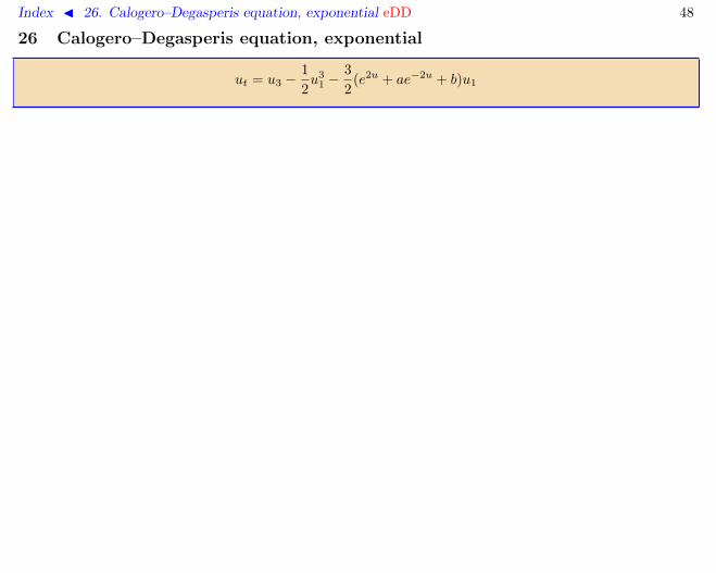
26 Calogero–Degasperis equation, exponential

ut = u3 −1

2u3

1 −3

2(e2u + ae−2u + b)u1

Index J 27. Calogero–Moser model D 49

27 Calogero–Moser model

qk = −∑j 6=k

f ′(qk − qj), j, k = 1, . . . , n, f(x) =

gx−2 rational case

sinh−2 x hyperbolic case

℘(x) elliptic case

ã Lax pair L = [L,A] for the rational case [2]:

Lij = piδij +(−g)1/2

qi − qj(1− δij), pi = qi, (−g)−1/2Aij = δij

∑k 6=i,j

1

(qi − qk)2− (1− δij)

1

(qi − qj)2.

See also: Ruijsenaars–Schneider model

References

[1] F. Calogero. Exactly solvable one-dimensional many-body problems. Lett. Nuovo Cimento 13:11 (1975) 411–416.

[2] J. Moser. Three integrable Hamiltonian systems connected with isospectral deformations. Adv. Math. 16 (1975)197–220.

[3] H. Airault, H.P. McKean, J. Moser. Rational and elliptic solutions of the KdV equation and a related many-bodyproblem. Comm. Pure Appl. Math. 30:1 (1977) 94–148.

[4] M.A. Olshanetsky, A.M. Perelomov. Classical integrable finite dimensional systems related to Lie algebras. Phys.Reports 71:5 (1981) 313–400.

Index J 28. Camassa–Holm equation DD 50

28 Camassa–Holm equation

ut − uxxt + 2kux = uuxxx + 2uxuxx − 3uux

ã Zero curvature representation:

ψxx =(λ(u− uxx + k) +

1

4

)ψ, ψt =

ux2ψ +

( 1

2λ− u)ψx

References

[1] R. Camassa, D.D. Holm. An integrable shallow water equation with peaked solitons. Phys. Rev. Let. 71:11(1993) 1661–1664.

[2] A.S. Fokas, B. Fuchssteiner. Symplectic structures, their Backlund transformations, and hereditary symmetries.Physica D 4:1 (1981) 47–66.

[3] R. Camassa, D.D. Holm, J.M. Hyman. A new integrable shallow water equation. Adv. Appl. Mech. 31 (1994)1–33.

[4] C.R. Gilson, A. Pickering. Factorization and Painleve analysis of a class of nonlinear third-order partial differ-ential equations. J. Phys. A 28:10 (1995) 2871–2888.

Index J 29. Cellular automata 51

29 Cellular automata

In the wide sense, a cellular automaton is a dynamical system with time and spatial independent variablestaking integer values and dependent variables taking values in some finite set. In the narrow sense, it isrequired that the dynamics is described locally. This means that the rules of transition t → t + 1 must bedetermined by the values of dependent variables in some neighborhood of any node of the spatial lattice.

ã Example: box-ball system.

Index J 30. Chen–Lee–Liu system eDD 52

30 Chen–Lee–Liu system

ut = uxx + 2uvux, vt = −vxx + 2uvvx

Alias: DNLS-II

ã Backlund transformation:

un,x = (unvn+1 + βn)(un+1 − un), vn,x = (un−1vn + βn−1)(vn − vn−1)

ã Nonlinear superposition principle:

un = un + (βn+1 − βn)un−1 − un

βn + un−1vn+1, vn = vn − (βn+1 − βn)

vn+1 − vnβn−1 + un−1vn+1

ã Zero curvature representation:

U =

(r λuλv −r

), V = 2rU +

(12 (uxv − uvx) λux−λvx 1

2 (uvx − uxv)

), 2r = uv − λ2

Ln = (unvn+1 + βn)−12

(unvn+1 + βn − λ2 λun

λvn+1 βn

)ã A multifield generalization [2, 3]: let u, v belong to an associative algebra, then the system

ut = uxx + 2uxvu, vt = −uxx + 2vuvx

possesses the third order symmetry

ut3 = uxxx + 3uxxvu+ 3uxvux + 3uxvuvu, vt3 = vxxx − 3vuvxx − 3vxuvx + 3vuvuvx.

In the case u ∈ MatM,N , v ∈ MatN,M the M ×M matrices

U = −2uxv, W = 2uxvx − 2uxxv − 4uxvuv

Index J 30. Chen–Lee–Liu system eDD 53

satisfy the matrix KP equation

4Ut3 = Uxxx − 3(UxU + UUx −Wt + [W,U ]), Wx = Ut

while the N ×N matricesF = vu, P = vux − vxu+ F 2

satisfy the matrix mKP equation

4Ft3 = Fxxx + 3([Fxx, F ]− 2FFxF + Pt + [P, F 2] + FxP + PFx), Ft = Px + [P, F ].

References

[1] H.H. Chen, Y.C. Lee, C.S. Liu. Integrability of nonlinear Hamiltonian systems by inverse scattering method.Physica Scr. 20 (1979) 490–492.

[2] P.J. Olver, V.V. Sokolov. Integrable evolution equations on associative algebras. Commun. Math. Phys. 193:2(1998) 245–268.

[3] P.J. Olver, V.V. Sokolov. Non-abelian integrable systems of the derivative nonlinear Schrodinger type. InverseProblems 14:6 (1998) L5–L8.

Index J 31. Chiral fields equation hDD 54

31 Chiral fields equation

ux = [u, Jv], vy = [v, Ju], u, v ∈ R3, |u| = |v| = 1, J = diag(a, b, c).

The linear in λ Lax pair found in [1] (up to the change to light-cone variables; u = (u1, u2, u3), v =(v1, v2, v3)):

U =

0 u1 u2 u3

−u1 0 u3 −u2

−u2 −u3 0 u1

−u3 u2 −u1 0

J , V =

0 v1 v2 −v3

−v1 0 v3 v2

−v2 −v3 0 −v1

v3 −v2 v1 0

J ,

J = λI − 1

2diag(c− a− b, b− a− c, a− b− c, a+ b+ c).

Backlund transformation and discretization were found in [2].

References

[1] L.A. Bordag, A.B.Yanovski. Polynomial Lax pairs for the chiral O(3)-field equations and the Landau–Lifshitzequation. J. Phys. A 28:14 (1995) 4007–4013.

[2] F.W. Nijhoff, V.G. Papageorgiou. Lattice equations associated with the Landau–Lifshitz equations. Phys. Lett.A 141:5–6 (1989) 269–274.

Index J 32. Chiral fields equation, principal hDD 55

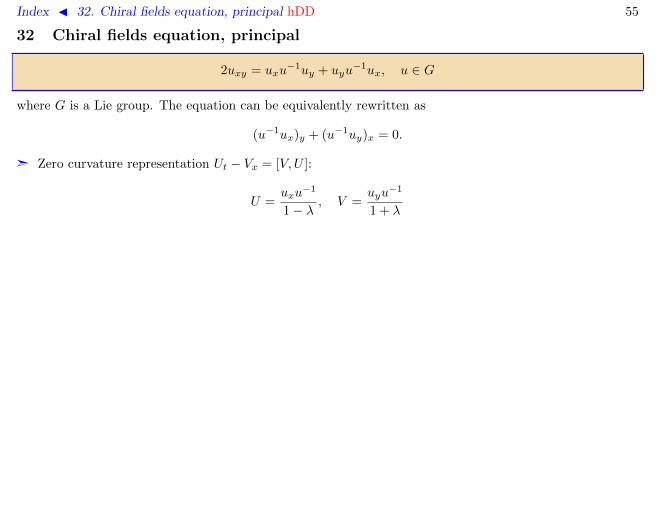
32 Chiral fields equation, principal

2uxy = uxu−1uy + uyu

−1ux, u ∈ G

where G is a Lie group. The equation can be equivalently rewritten as

(u−1ux)y + (u−1uy)x = 0.

ã Zero curvature representation Ut − Vx = [V,U ]:

U =uxu

−1

1− λ, V =

uyu−1

1 + λ

Index J 33. Classical symmetry 56

33 Classical symmetry

A classical symmetry is a local one-parametric group of point or contact transformations which preservethe equation under scrutiny. This notion is wide applicable to all sorts of partial and ordinary differen-tial/difference equations.

The theory of classical symmetries was developed by Lie. The modern treatment of the classical and thegeneralized evolutionary symmetries can be found in the references below.

References

[1] R.L. Anderson, N.H. Ibragimov. Lie–Backlund transformations in applications. Philadelphia: SIAM, 1979.

[2] N.H. Ibragimov. Transformation groups applied to mathematical physics. Dordrecht: Reidel, 1985.

[3] P.J. Olver. Applications of Lie groups to differential equations, 2nd ed., Graduate Texts in Math. 107, NewYork: Springer-Verlag, 1993.

[4] L.V. Ovsyannikov. Group analysis of differential equations, New York: Academic Press, 1982.

[5] V.V. Sokolov. On the symmetries of evolution equations. Russ. Math. Surveys 43:5 (1988) 165–204.

Index J 34. Collapse 57

34 Collapse

Author: Yu.N. Ovchinnikov, 10.09.2007

The scenarios of collapse in the Cauchy problem for Nonlinear Schrodinger equation

iut = ∆u+ |u|ρu ⇒ d

dt

∫|u|2dx = 0, x ∈ Rn

were studied in [1, 2, 3, 4, 5, 6, 8, 9, 10, 11, 12, 13]. The use of Sobolev embedding theorems allows to proveat n = 2, 3 the existence of the local solutions of this problem in the following cases:

n = 2, 1 ≤ ρ or n = 3, 1 ≤ ρ < 4 ⇒ u ∈ C([0, t0)) ∩W 22 ∩ u|ru ∈ L2.

Let us use the energy conservation law

E(t) =

∫|ux|2dx−

2

ρ+ 2

∫|u|ρ+2dx = E0 = const, (1)

φ(t) ≤ 4E0t2 + 4µt+ φ(0), φ :=

∫r2|u|2dx.

The second term in (1) can be estimated as follows, for u ∈W 1;02 (Rn), n ≥ 2 and 0 ≤ α < 1:

||u||q ≤ β||ux||α||u||1−α,1

q=

1

2− α

n, and ||u||6 ≤ β||ux||1/3||u||2/34 , n = 2 (2)

and this allows to prove the global solvability of the Cauchy problem at ρ < ρ0, ρ0 = 4n . Indeed, due to (2)∫

|u|qdx = ||u||qq ≤ β||ux||qα||u||q−qα and qα = 1 ⇒ ρ = q − 2 =4

n.

At ρ = ρ0 the problem on the collapse admits an explicit solution [14]

u(t, x) = (t0 − t)−n/4v(ξ) exp(iαr2 + βt

t0 − t

), ξ =

r

t0 − t, v(ξ) > 0,

Index J 34. Collapse 58

vξξ +n− 1

ξvξ + λv = 0, inf||w||p : ||∇w||2 − 2

σ||w||σσ ≤ 0, σ = ρ+ 2, ρ =

4

n.

This scenario is not unique (see multi-particle solutions in [15, 16, 17]).At ρ 6= ρ0 the problem on the collapse does not admit selfsimilar solutions which vanish at infinity.

Similarity Ansatz yields

|u|2 = (t0 − t)−n/2ξ1−nAξ(ξ), ξ :=r√t0 − t

,

Aξξξ =A2ξξ

2Aξ+Aξ

(n2 − 4n+ 3

2ξ2+ξ2

4+ 2

(Aξξn−1

)ρ/2+ c

)+ ε

ξA

2+ ε2 A

2

8Aξ, ε =

4

ρ− n.

References

[1] I.M. Sigal. Non-linear semi-groups. Ann. Math. 78 (1963) 339–364.

[2] A.V. Zhiber. The collapse of solutions of one nonlinear boundary value problem. Proc. of the conference onPDE, Moscow State University (1978) 78–79.

[3] C. Sulen, P. Sulen. The NLSE: self-focusing ans wave collapse. New York: Springer, 1999.

[4] Yu.N. Ovchinnikov. Weak collapse in the nonlinear Schrodinger equation. JETP Lett. 69:5 (1999) 418–422.

[5] Yu.N. Ovchinnikov, I.M. Sigal. Collapse in the Nonlinear Schrodinger equation. JETP 89:1 (1999) 5–40.

[6] Yu.N. Ovchinnikov, I.M. Sigal. Optical bistability. JETP 93:5 (2001) 1004–1016.

[7] Yu.N. Ovchinnikov, I.M. Sigal. The energy of Ginzburg–Landau vortices. J. of Appl. Math. 13 (2002) 153.

[8] Yu.N. Ovchinnikov, I.M. Sigal. Collapse in the Nonlinear Schrodinger equation of critical dimension. JETP Lett.75:7 (2002) 357–361.

[9] Yu.N. Ovchinnikov, I.M. Sigal. Multiparameter family of collapsing solutions to the critical NonlinearSchrodinger equation in dimension D = 2. JETP 97:1 (2003) 194–203.

[10] Yu.N. Ovchinnikov, V.L. Vereshchagin. Asymptotic behavior of weakly collapsing solutions of the nonlinearSchrodinger equation. JETP Lett. 74:2 (2001) 72–76.

Index J 34. Collapse 59

[11] Yu.N. Ovchinnikov, V.L. Vereshchagin. The properties of weakly collapsing solutions to the nonlinear Schrodingerequation at large values of free parameters. JETP 93:6 (2001) 1307–1313.

[12] Yu.N. Ovchinnikov. Properties of weakly collapsing solutions to the nonlinear Schrodinger equation. JETP Lett.96:5 (2002) 975–981.

[13] P. Bizon, Yu.N. Ovchinnikov, I.M. Sigal. Collapse of instanton. Nonlinearity 17:4 (2004) 1179–1191.

[14] V.I. Talanov. JETP Lett. 11 (1970) 303.

[15] M.I. Weinstein. Nonlinear Schrodinger equations and sharp interpolation estimates. Commun. Math. Phys. 87:4(1982) 567–576.

[16] M.I. Weinstein. Comm. Partial Diff. Eqs 11 (1986) 545–565.

[17] H. Nawa. Asymptotic and limiting profiles of blow up solutions of the nonlinear Schrodinger equation withcritical power. Comm. Pure and Appl. Math. 52:2 (1999) 193–270.

Index J 35. Conservation law 60

35 Conservation law

Conservation law is an equality of the form divF = 0 which turns into identity on any solution of a givenPDE. Conservation law is called trivial

1) either if F itself vanishes on the solutions2) or if divF vanishes identically (independently on the equation).

Clearly, all conservation laws form a linear space and it is only the factor-space what makes sense, modulotrivial conservation laws. The order of the conservation law is defined as the minimal order with respect toderivatives in the class of equivalence.

ã Example: consider equation of the form uxt = f ′(u). It admits the conservation laws

Dt(u2xt − f ′(u)2 + ux) = Dx(ut), Dt(u

2x) = Dx(2f(u)).

The first equality is a combination of two types of trivial conservation laws; the second one is nontrivialconservation law of first order.

ã In the case of evolutionary PDE the time-component is often written separately, so that conservationlaws take the form Dt(ρ) = divx(σ), where function ρ is called density and vector σ is called flux of theconservation law. Integration over some spatial domain yields, under suitable boundary condition, theintegral constant of motion

∫Ωρ dx = const.

The notion of the order can be formalized by use of variational derivative. In the simplest case ofscalar evolutionary equations with one spatial variable, the order of a conservation law with the densityρ = ρ(x, u, . . . , um) is equal to one half of the order of the expression

δρ

δu= ρu −D(ρu1

) +D2(ρu2)− · · ·+ (−D)m(ρum

).

This does not depend on the addition of type 2) trivial conservation laws, and type 1) is excluded byrequirement that ρ does not depend on t-derivatives.

Index J 35. Conservation law 61

References

[1] P.J. Olver. Applications of Lie groups to differential equations, 2nd ed., Graduate Texts in Math. 107, NewYork: Springer-Verlag, 1993.

Index J 36. Contact transformations 62

36 Contact transformations

In the case of one dependent variable (m = 1) the point transformations can be generalized as follows. Letp = (p1, . . . , pn), pi = ∂u/∂xi. The contact transformation is a nondegenerate transformation of theform

Xi = Xi(x, u, p), U = U(x, u, p), Pi = Pi(x, u, p) (1)

where functions Xi, U, Pi are related in such a way that the total differential is preserved:

dU −∑

PidXi = c(du−∑

pidxi), c = c(x, u, p) 6= 0.

More explicitly, this condition is equivalent to the following set of equations:

Xi, Xj = 0, Pi, Pj = 0, Pi, Xj = δijc, Xi, U = 0, Pi, U = cPi,

where

f, g =

n∑i=1

(fpi(gxi+ pigu)− gpi(fxi

+ pifu)).

Note the relation[Xf , Xg] = Xf,g

which is valid for the contact vector fields

Xf =∑i

fpi∂xi−∑i

(fxi+ pifu)∂pi +

(∑i

pifpi − f)∂u.

ã Example. Point and contact transformations of the evolutionary equations. As an illustrativeexample, consider in more details the case of evolutionary 1 + 1-dimensional equations

ut = F (t, x, u, u1, . . . , un), uk = Dkx(u).

It is easy to show that the subgroup of the contact transformations preserving the evolutionary form is givenby the formulae

T = T (t), X = X(t, x, u, u1), U = U(t, x, u, u1)

Index J 36. Contact transformations 63

where the functions T,X,U satisfy the conditions

T ′ 6= 0, Dx(X) 6= 0, w = Uu −Uu1

Xu1

Xu 6= 0, Xu1(Ux + Uuu1) = Uu1(Xx +Xuu1).

The prolongation of this transformation on the x-derivatives is given by the formula

U1 =Ux + Uuu1

Xx +Xuu1=Uu1

Xu1

, Uk = Uk(t, x, u, . . . , uk) = DkX(U), DX =

1

Dx(X)Dx

and the equation UT = F (T,X,U, . . . , Un) transforms into

ut = f(t, x, u, . . . , un) = w−1(T ′F − Ut + U1Xt).

The following formula is valid for the transformations of this type at k > 1:

Uk,uk=

w

(Dx(X))k. (2)

In particular, at n ≥ 2fun = T ′(Dx(X))−nFUn

The formula (2) it is valid also at k = 1 for the subgroup of the point transformations

T = T (t), X = X(t, x, u), U = U(t, x, u),

and it is valid also at k = 0 (w = Uu) for the transformations of the form

T = T (t), X = X(t, x), U = U(t, x, u).

References

[1] N.H. Ibragimov. Transformation groups applied to mathematical physics. Dordrecht: Reidel, 1985.

Index J 37. Darboux transformation 64

37 Darboux transformation

Let us consider the Sturm–Liouville spectral problem

ψxx = (u(x)− λ)ψ. (1)

Statement 1 (Darboux transformation [1]). Equation (1) is form invariant under the transformation

ψ = ψx − fψ, u = u− 2fx, f := ψ(α)x /ψ(α) (2)

where ψ(α) is a particular solution of (1) at λ = α.

The function f satisfies the Riccati equations

fx + f2 = u− α, −fx + f2 = u− α.

The iteration of Darboux transformation brings to the sequence of operators Ln = −D2x+un, An = −Dx+fn

related by equations

Ln = A+nAn + αn → Ln+1 = AnA

+n + βn = A+

n+1An+1 + αn+1.

This sequence is governed by the dressing chain

fn,x + fn+1,x = f2n − f2

n+1 + αn − αn+1.

Any solution of this differential-difference equation generates a family of the operators Ln with ψ-functionscalculated for all λ = βk explicitly:

ψk,k = exp(

∫fkdx), ψn,k = A+

nψn+1,k, n < k. (3)

This feature explains the role of Darboux transformation in quantum mechanics, see factorization method.Darboux transformation admits straightforward generalizations for linear problems of any order and in

any dimension. We mention here few most typical examples. In particular, the above transform can beeasily obtained by separation of variables from the following one.

Index J 37. Darboux transformation 65

Statement 2. The 2-dimensional Schrodinger equation

σψy = ψxx − u(x, y)ψ (4)

is form invariant under the transformation

ψ = ψx − fψ, u = u− 2fx, f := φx/φ (5)

where φ is any particular solution of (4).

Proof. Denote g = φy/φ then gx = fy, σg = fx + f2 − u and

L = σDy −D2x + u = σ(Dy − g)− (Dx + f)(Dx − f), [Dy − g,Dx − f ].

Therefore ψ satisfies the equation Lψ = 0, where L = σ(Dy − g)− (Dx − f)(Dx + f) = L− 2fx.

Iterations of the transform (5) are governed by the 2D dressing chain

fn,x + fn+1,x = f2n − f2

n+1 − σ(gn − gn+1), gn,x = fn,y.

References

[1] G. Darboux. Compt. Rend. 94 1456–1459.

Index J 38. Darboux system hDDD 66

38 Darboux system

uijxk= uikukj , i 6= j 6= k 6= i

Alias: Darboux–Zakharov–Manakov system

ã The system is the consistency condition of the linear equations

ψixj= uijψj , i 6= j.

The flows Dxk, Dxm

commute: uijxk,xm= uijxm,xk

.

References

[1] G. Darboux. Lecons sur les systemes orthogonaux et les coordonnees curvilignes. 2 ed., Paris: Gauthier-Villars,1910.

[2] V.E. Zakharov, S.V. Manakov. Funct. Anal. Appl. 19 (1985) 11.

Index J 39. Darboux system discrete h∆∆∆ 67

39 Darboux system discrete

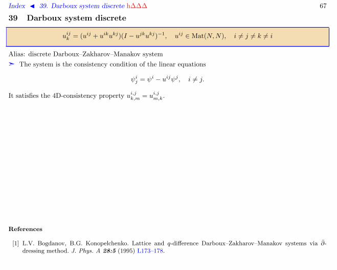
uijk = (uij + uikukj)(I − ujkukj)−1, uij ∈ Mat(N,N), i 6= j 6= k 6= i

Alias: discrete Darboux–Zakharov–Manakov system

ã The system is the consistency condition of the linear equations

ψij = ψi − uijψj , i 6= j.

It satisfies the 4D-consistency property ui,jk,m = ui,jm,k.

References

[1] L.V. Bogdanov, B.G. Konopelchenko. Lattice and q-difference Darboux–Zakharov–Manakov systems via ∂-dressing method. J. Phys. A 28:5 (1995) L173–178.

Index J 40. Davey–Stewartson system eDDD 68

40 Davey–Stewartson system

ut+ = uxx + 2pxu, −vt+ = vxx + 2pxv, py = uv

ut− = uyy + 2qyu, −vt− = vyy + 2qyv, qx = uv

ã Derived in [1] by multiscale analysis of modulated nonlinear surface gravity waves propagating over ahorizontal sea bed. DS system is a two-dimensional analog of nonlinear Schrodinger equation.

ã The flows ∂t+ , ∂t− commute. Any linear combination α∂t+ + β∂t− is called DS system as well.

ã The auxiliary linear problems [2, 3]:ψy = uφφx = −vψ

ψt+ = ψxx + 2pxψφt+ = vxψ − vψx

−ψt− = uφy − uyφ−φt+ = φyy + 2qyφ

ã Gauge equivalent systems are the Ishimori equation and the 2D Reyman system.

ã Third order symmetry:

ut3 = uxxx + 3uxD−1y (uv)x + 3uD−1

y (uxv)x,

vt3 = vxxx + 3vxD−1y (uv)x + 3vD−1

y (uvx)x.(1)

It admits reductions v = 1 to the Veselov–Novikov equation and u = v to the modified Veselov–Novikovequation.

References

[1] A. Davey, K. Stewartson. On three dimensional packets of surface waves. Proc. R. Soc. A 338 (1974) 101–110.

[2] M. Boiti, J.J.-P. Leon, L. Martina, F. Pempinelli. Scattering of localized solitons in the plane. Phys. Lett. A132:8–9 (1988) 432–439.

[3] M. Boiti, L. Martina, F. Pempinelli. Multidimensional localized solitons. Chaos, Solitons and Fractals 5:12(1995) 2377–2417.

Index J 41. Davey–Stewartson system matrix eDD 69

41 Davey–Stewartson system matrix

ut = uxx + 2wu, −vt = vxx + 2vw, wy = (uv)x, u, vᵀ ∈ Mat(m,n), w ∈ Mat(m,m)

ã This and some other analogous examples were introduced in [1].

ã The linear problem (ψ ∈ Rm, φ ∈ Rn):

ψy = uφ, φx = −vψ, ψt = ψxx + 2wψ, φt = vxψ − vψx.

References

[1] C. Athorne, A.P. Fordy. Integrable equations in (2+1) dimensions associated with symmetric and homogeneousspaces. J. Math. Phys. 28:9 (1987) 2018–2024.

Index J 42. Degasperis–Procesi equation DD 70

42 Degasperis–Procesi equation

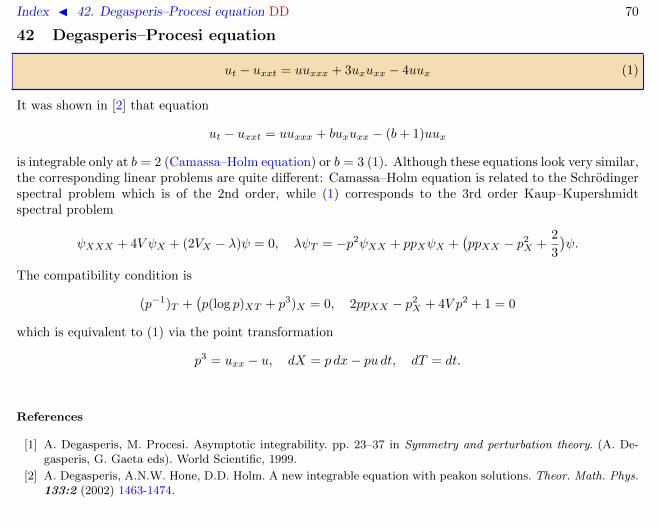
ut − uxxt = uuxxx + 3uxuxx − 4uux (1)

It was shown in [2] that equation

ut − uxxt = uuxxx + buxuxx − (b+ 1)uux

is integrable only at b = 2 (Camassa–Holm equation) or b = 3 (1). Although these equations look very similar,the corresponding linear problems are quite different: Camassa–Holm equation is related to the Schrodingerspectral problem which is of the 2nd order, while (1) corresponds to the 3rd order Kaup–Kupershmidtspectral problem

ψXXX + 4V ψX + (2VX − λ)ψ = 0, λψT = −p2ψXX + ppXψX +(ppXX − p2

X +2

3

)ψ.

The compatibility condition is

(p−1)T +(p(log p)XT + p3)X = 0, 2ppXX − p2

X + 4V p2 + 1 = 0

which is equivalent to (1) via the point transformation

p3 = uxx − u, dX = p dx− pu dt, dT = dt.

References

[1] A. Degasperis, M. Procesi. Asymptotic integrability. pp. 23–37 in Symmetry and perturbation theory. (A. De-gasperis, G. Gaeta eds). World Scientific, 1999.

[2] A. Degasperis, A.N.W. Hone, D.D. Holm. A new integrable equation with peakon solutions. Theor. Math. Phys.133:2 (2002) 1463-1474.

Index J 43. Differential and pseudo-differential operators 71

43 Differential and pseudo-differential operators

Author: A.B. Shabat, 28.04.2007

1. The problem on commuting differential operators2. The field of pseudo-differential operators3. Burchnall–Chaundy theorem4. Residues

The role of the differential operators is explained by the fact that the construction problems of finite-gappotentials and higher symmetries of integrable equations are formulated on this language. In both cases,the introducing of pseudo-differential operators is useful. In particular, this is important in the theories ofrecursion operators and formal symmetry.

1. The problem on commuting differential operators

Multiplication in the ring R of the differential operators (DO)

A =

n∑k=0

an−kDk = a0D

n + a1Dn−1 + a2D

n−2 + · · ·+ an, D ≡ d

dx

with smooth coefficients ak = ak(x) is defined by the Leibniz rule

Dma = aDm +maxDm−1 +

m(m− 1)

2axxD

m−2 + . . . .

If A = a0Dn + . . . and B = b0D

m + . . . then

[A,B] := AB −BA = (na0b0,x −mb0a0,x)Dn+m−1 + . . . (1)

so that, generally, the order of commutator is n+m− 1. Therefore, the commutativity condition [A,B] = 0is equivalent to a system of n+m equations for n+m+2 coefficients of A and B. The numbers of equationsand unknowns become balanced if we introduce two basic transformations as follows

D = aD, A = f−1Af. (2)

Index J 43. Differential and pseudo-differential operators 72

The first transformation corresponds to the change of the independent variable x → x and the secondone is the conjugation with the zero order operator of multiplication by a smooth function f = f(x).Both transformations preserve the property of commutativity. For example, in the case of the conjugationAB = AB and thus

[A,B] = 0 ⇔ [A, B] = 0.

The change of independent variable with a = a1/n0 replaces A by the operator A with the leading coefficient

a0 = 1.

Definition 1. Centralizer C(A) of a DO A is the subring of DOs commuting with A:

C(A) = B ∈ R : [A,B] = 0.

Centralizer is called trivial if it consists of polynomials with constant coefficients in some minimal orderdifferential operator C, that is

A = α0Cn + α1C

n−1 + · · ·+ αn, B = β0Cm + β1C

m−1 + · · ·+ βm, αi = const, βi = const .

It is easy to prove that the centralizer of a first order DO is always trivial. Indeed, if A = a0D+ a1 thentransformations (2) allow to reduce it to A = D. Since

[D, b0Dm + b1D

m−1 + · · ·+ bm] = D(b0)Dm +D(b1)Dm−1 + · · ·+D(bm),

hence all bi are constant. Thus, in nontrivial cases the order n of the operator A must be at least 2. In theexample below n = 2 and order of B is chosen minimal as well.

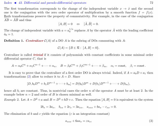
Example 2. Let A = D2 +a and B = D3 + bD+ c. Then the equation [A,B] = 0 is equivalent to the system

2bx = 3ax, bxx + 2cx = 3axx, axxx + bax − cxx = 0.

The elimination of b and c yields the equation (ε is an integration constant)

axxx + 6aax = εax, (3)

Index J 43. Differential and pseudo-differential operators 73

Any solution of this equation gives rise to a commuting pair of DOs. Moreover, it is easy to check that ifu 6= const then no first order operator C exists such that A = α0C

2 + α1C + α2, so that this pair is nottrivial. Particularly, the choice u = 2x−2 yields the pair

A = D2 − 2x−2, B = D3 − 3x−2D + 3x−3, [A,B] = 0, A3 = B2.

2. The field of pseudo-differential operators

In order to understand the structure of nontrivial centralizers we need to extend the ring R introducing thepseudo-differential operators (PDO) as the formal series

A = a0Dn + a1D

n−1 + a2Dn−2 + . . . (4)

The product in the extended ring R is defined by the Leibniz rule generalized for any integer power of D:

Dna =

∞∑k=0

(n

k

)Dk(a)Dn−k =

. . .

aD−1 − axD−2 + axxD−3 − . . . n = −1

aD−2 − 2axD−3 + 3axxD

−4 − . . . n = −2

aD−3 − 3axD−4 + 6axxD

−5 − . . . n = −3

. . .

where(nk

)= n(n − 1) · · · (n − k + 1)/k!. In particular, for the first order PDO with unit leading coefficient

B = D + b1 + b2D−1 + b3D

−2 + . . . we find

Bn = Dn + b1,nDn−1 + b2,nD

n−2 + b3,nDn−3 + . . . , b1,n = nb1,

b2,n = nb2 +

(n

2

)(b1,x + b21), b3,n = nb3 +

(n

2

)(b2,x + 2b1b2) +

(n

3

)(b1,xx + 3b1b1,x + b31), . . .

(5)

Therefore the expressions for the coefficients bj,n, j = 1, 2, . . . contain only first j coefficients of the given

series B. This triangular structure of the equations allows to introduce additional algebraic operations in R.

Index J 43. Differential and pseudo-differential operators 74

Lemma 3. Let A be a formal series (4) of order n with a0 = 1. Then:the unique formal series L = A−1 exists such that AL = LA = 1;if n 6= 0 then the unique formal series B = A1/n exists such that ordB = 1, the leading coefficient is 1

and Bn = A.

Proof. The proof is analogous in both cases and we consider only the second one. Starting with formulas(5) we have

bj,n = nbj + f [b1, b2, . . . , bj−1]

where f is a differential polynomial in its arguments. The system for the coefficients bk

a1 = nb1, a2 = b2,n, a3 = b3,n, . . .

is triangular and is solved uniquely.

Two series defined in Lemma are called inverse and n-th root correspondingly. The condition a0 = 1

is a technical one and the transformation D → aD (see (2)) with a = a1/n0 leads to a series A with unitary

leading coefficient.We would like to stress again that due to triangular structure of equations the first j coefficients of

the original series A define first j coefficients of series A−1 and A1/n. This recursive property of algebraicoperations in the field R of power series (4) appears to be very important.

3. Burchnal–Chaundy theorem

Now we can return to the commutativity problem. Consider the centralizer in the ring R:

C(A) = B ∈ R : [A,B] = 0.

The following statement shows that, in contrast to the case of DOs, this centralizer is always trivial.

Theorem 4 (Burchnal, Chaundy [1]). Let A ∈ R, ordA = n 6= 0. Then the PDO B ∈ R commutes with Aif an only if it can be represented as the formal series

B = β0Am1 + β1A

m−11 + . . . , βk = const, An1 = A. (6)

Index J 43. Differential and pseudo-differential operators 75

Proof. Obviously, any power of A1 commute with A and belongs to C(A). In order to prove the oppositestatement denote B1 = [B,A1]. Then

BA−AB = BAn1 −An1B = B1An−11 +A1B1A

n−21 + · · ·+An−1

1 B1 ⇒ C(A1) = C(A), (7)

since all n terms in the sum (7) have the same leading coefficient.

The leading coefficient b0 of the PDO B ∈ C(A1) of order m 6= 0 must be proportional to am0 , due to theformulae (1) which remains valid in R. Therefore, we find that

B ∈ C(A1) ⇒ b0 = β0am0 ⇒ B = B − β0A

m1 ∈ C(A1).

In order to finish the proof of we use the induction with respect to the order m < m of the series B =B−β0A

m1 . It remains to notice that in the case of order m = 0 with B = b0 + b1D

−1 the formula (1) impliesthat a0b0,x = 0. Thus in this case the series B = B − b0 has negative order and the inductive process meetsno obstacles.

It follows from the above theorem that any centralizer C(A) is abelian, that is

B1, B2 ∈ C(A) ⇒ [B1, B2] = 0.

In the case of a differential operator A the centralizer C(A) ⊂ C(A) and thus, we obtain a classical result asfollows.

Corollary 5. Any two differential operators commuting with a third one commute with each other.

In other words, the binary relation [A,B] = 0 is an equivalence and one can replace the operator A inC(A) by any nontrivial (of non zero order) element of the centralizer. The minimal order n > 0 of nontrivialelements of C(A) gives some indication on what is the structure of the centralizer. For n = 1 the centralizer isalways trivial, but in the case n = 2 there are nontrivial ones with odd order differential operators B ∈ C(A)(see Example 2). Moreover, although an element B ∈ C(A) generally cannot be represented as polynomialin A yet there exist an algebraic relation between A and B in virtue of Theorem 4.

Index J 43. Differential and pseudo-differential operators 76

Example 6. Let us consider tersely the structure of C(A) in the case of second order differential operator A. Ifthe centralizer is nontrivial then it contains a differential operator B1 of a minimal odd order 2n+1 ≥ 3. Anyelement in C(A) can be represented as P (A)B+Q(A) where P,Q are polynomials with constant coefficients.In particular, B2

1 = P (A)B1+Q(A) and replacing B1 = B+ 12P (A) we come to algebraic relation B2 = Q(A).

It is easy to see that the operator B is also of the minimal order 2n + 1, and this is also the degree of thepolynomial Q. The relation B2 = Q(A) completely defines the multiplication in the commutative ring C(A)with the generators A and B.

4. Residues

Due to Theorem 4 the structure of centralizer C(A) is related with the properties of the formal series

A1 = a0D + a1 + a2D−1 + a3D

−2 + . . . , An1 = A ∈ R. (8)

For any PDOB = b0D

n + b1Dn−1 + · · ·+ bn + bn+1D

−1 + . . . ∈ R

we define the differential part and residue

B+ := b0Dn + b1D

n−1 + · · ·+ bn ∈ R, res(B) := bn+1. (9)

Particularly, for the formal series (8) we denote

ρj = resAj1, j = −1, 1, 2, . . . , ρ0 = a1/a0. (10)

Inverse above formulae one finds (see (5)) that

a0 = 1/ρ−1, a1 = ρ0/ρ−1, a2 = ρ1, 2a3 = ρ3ρ−1 − 2ρ1ρ0 −(ρ1ρ−1)xρ−1

, . . .

and the recursive properties of algebraic operations in R allows to prove easily (see [2]) the following Lemma.

Lemma 7. The sequence (10) of the residues of powers of A1 and the sequence of coefficients of this formalseries defines each other uniquely and recursively.

Index J 43. Differential and pseudo-differential operators 77

Definition 8. For a differential operator L = Dm + l2Dm−2 + · · · + lm of the special form we call by

L-hierarchy the sequence (10) of residues ρj = ρj(L), j ≥ 1 expressed in terms of coefficients l2, . . . , lm ofthe differential operator L.

Example 9. In the case of the second order DO L = D2 + a the coefficients of the series A ∈ R, A2 = L areexpressed through a:

A = D + a1D−1 + a2D

−2 + . . . , 2a1 = a, 4a2 = −ax, 8a3 = axx − a2,

16a4 = −axxx + 6aax, 25a5 = axxxx + 2a3 − 14aaxx − 11a2x, . . .

(11)

That gives for residues ρj(a) = ρj(L) with odd j = 1, 3, 5, . . .

2ρ1(a) = a, 23ρ3(a) = axx + 3a2, 25ρ5(a) = axxxx + 5a2x + 10aaxx + 10a3, . . . (12)

All even residues vanish ρ2n(a) = 0, n = 1, 2, 3, . . . because for even powers of series (11) A2n = Ln.One finds by substitution of the expansion (9) into the formula [L,Aj ] = 0:

Aj = (Aj)+ + ρjD−1 +O(D−2) ⇒ [L, (Aj)+] = −2ρj,x, (13)

since (cf (1))

0 = [L,Aj ] = [L, (Aj)+] + [L, ρjD−1] +O(D−1) = [L, (Aj)+] + 2ρj,x +O(D−1).

Summing up, we see that above definition of L-hierarchy together with Theorem 4 and formula (13) allowto formulate a criterium of non-triviality of the centralizer C(L) of a differential operator L = D2 + a of thesecond order.

Corollary 10 (of Theorem 4). The centralizer C(D2 +a) is non-trivial if and only if it contains a differentialoperator B of odd order 2n+ 1, n ≥ 1 and in this case the function a = a(x) satisfies the nonlinear ODE oforder 2n+ 1 :

ρ2n+1(a) +

n−1∑k=0

ckρ2k+1(a) = cn, cj = const ∈ C.

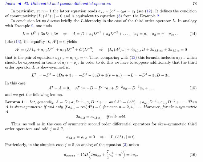
Index J 43. Differential and pseudo-differential operators 78

In particular, at n = 1 the latter equation reads axx + 3a2 + c0a = c1 (see (12). It defines the conditionof commutativity [L, (A3)+] = 0 and is equivalent to equation (3) from the Example 2.

In conclusion let us discuss briefly the L-hierarchy in the case of the third order operator L. In analogywith Example 9, one finds

L = D3 + 3uD + 3v ⇒ A = D + a1D−1 + a2D

−2 + . . . , a1 = u, a2 = v − ux, . . . (14)

Like (13), the equality [L,Aj ] = 0 yields

Aj = (Aj)+ + aj,1D−1 + aj,2D

−2 +O(D−3) ⇒ [L, (Aj)+] + 3aj,1,xD + 3aj,1,xx + 3aj,2,x = 0

that is the pair of equations aj,1,x = aj,2,x = 0. Thus, comparing with (13) this formula includes aj,2,x whichshould be expressed in terms of aj,1 = ρj . In order to do this we have to suppose additionally that the thirdorder operator L is skew-symmetric:

Lᵀ := −D3 − 3Du+ 3v = −D3 − 3uD + 3(v − ux) = −L = −D3 − 3uD − 3v.

In this caseAᵀ +A = 0, Aᵀ := −D −D−1a1 +D−2a2 −D−3a3 + . . . (15)

and we get the following lemma.

Lemma 11. Let, generally, A = D+a1D−1+a2D

−2+. . . and An = (An)++an,1D−1+an,2D

−2+. . . . ThenA is skew-symmetric if and only if an,1 = res(An) = 0 for even n = 2, 4, . . . . Moreover, for skew-symmetricA

2an,2 = an,1,x, if n is odd.

Thus, as well as in the case of symmetric second order differential operators for skew-symmetric thirdorder operators and odd j = 5, 7, . . .

aj,1,x = ρj,x = 0 ⇒ [L, (Aj)+] = 0.

Particularly, in the simplest case j = 5 an analog of the equation (3) arises

uxxxxx + 15D(

2uuxx +7

4u2x + u3

)= εux. (16)

Index J 43. Differential and pseudo-differential operators 79

The calculation of res(A5) is long enough and, as a matter of fact, it is comparable with straightforwardcomputation of the commutator [L,M ] = a1D + a2 where

L = D3 + 3uD + 3v, M = (A5)+ = D5 + 5uD2 + aD + b+ c.

These computations give firstly

a = 5(ux + v), 3b = 10uxx + 15u2 + 15vx, 3c = 10vxx + 30uv

and the condition [L,M ] = 0 results now in the pair of equationsuxxxxx + 15D(uuxx + u2

x + 3vux − 3v2 + u3) = εux,

vxxxxx + 15D(uvxx + 2vuxx + 2vxux − 3vvx + 3u2v) = εvx.(17)

It is easy to see that the fifth order equation (16) for u represents one of three possible scalar reductionsδv = ux, δ = 0, 1, 2 of this system.

References

[1] J.L. Burchnall, T.W. Chaundy. Commutative ordinary differential operators. Proc. London Soc. Ser. 2 21 (1923)420–440.

[2] A.V. Mikhailov, A.B. Shabat, R.I. Yamilov. The symmetry approach to classification of nonlinear equations.Complete lists of integrable systems. Russ. Math. Surveys 42:4 (1987) 1–63.

Index J 44. Differential substitutions 80

44 Differential substitutions

The formulae (186.2), (186.3) define the prolongation also for transformations more general than the pointones:

xi = fi(x, us), uj = gj(x, us), |s| ≤ k. (1)

Theorem 1 (Backlund [1, 2]). Let the prolongation of the transformation (1) be invertible on some Jr.Then it is point if m > 1 or contact if m = 1.

The transformations (1) which are not point or contact are called differential substitutions. It shouldbe stressed that Backlund theorem does not mean that any such transformation is not invertible. Forexample, the following transformation is involutive:

x = x, u =vxux, v = −v + u

vxux.

However, it is easy to see that its prolongation does not define an invertible transformation of Jr, for anyfinite r.

Examples: see substitutions for the Bogoyavlensky–Narita lattices and for the KdV-type equations.

References

[1] A.V. Backlund. Einigies uber Curven- und Flachentransformationen. Lunds Universitets Ars-skrift 10 (1873)1–12.

[2] A.V. Backlund. Uber Flachentrasformationen. Math. Ann. 9:3 (1875) 297–320.

Index J 45. Discrete differential geometry 81

45 Discrete differential geometry

This field deals with discretization of several notions first discovered within the framework of classicaldifferential geometry in the beginning of the 20-th century [1, 2, 3, 4, 5]. These include many specialclasses of surfaces and coordinate systems, such as minimal surfaces, surfaces with constant mean curvature,isothermic surfaces, orthogonal and conjugate coordinate systems and more, and also transformations ofthese objects.

Understanding of classical results from the point of view of modern theory of integrability became pos-sible, in particular, due to the progress in construction of their discrete analogues. The objects of discretedifferential geometry are discrete nets, that is, mappings from ZM into Rd (or some other suitable space)specified by certain geometric properties. Their study was initiated in [6, 7]. More recently, the key obser-vation was made that discretization can be defined in terms of Backlund–Darboux type transformations andBianchi permutability property for the continuous objects. On the other hand, continuous objects can bereproduced from the discrete ones under a suitable limit. In many aspects, the discrete picture turns out tobe more transparent and fundamental than the continuous one since the transformations of discrete surfacesare described by the same equations as surfaces themselves. This scheme was realized in various settings inthe papers [8, 9, 10, 11], see also the book [12] for more details and further references.

References

[1] L. Bianchi. Lezioni di geometria differenziale. 3 ed., Pisa: Enrico Spoerri, 1923.

[2] G. Darboux. Lecons sur les systemes orthogonaux et les coordonnees curvilignes. 2 ed., Paris: Gauthier-Villars,1910.

[3] G. Darboux. Lecons sur la theorie generale des surfaces et les applications geometriques du calcul infinitesimal.T. I-IV. 3 ed., Paris: Gauthier-Villars, 1914-1927.

[4] L.P. Eisenhart. A treatise on the differential geometry of curves and surfaces. Boston: Ginn, 1909.

[5] L.P. Eisenhart. Transformations of surfaces. Princeton University Press, 1923.

[6] R. Sauer. Differenzengeometrie. Berlin: Springer-Verlag, 1970.

Index J 45. Discrete differential geometry 82

[7] W. Wunderlich. Zur Differenzengeometrie der Flachen konstanter negativer Krummung. Osterreich. Akad. Wiss.Math.-Nat. Kl. 160 (1951) 39–77.

[8] A.I. Bobenko, U. Pinkall. Discrete surfaces with constant negative Gaussian curvature and the Hirota equation.J. Differential Geom. 43:3 (1996) 527–611.

[9] A.I. Bobenko, U. Pinkall. Discrete isothermic surfaces. J. Reine Angew. Math. 475 (1996) 187–208.

[10] A. Doliwa, P.M. Santini. Multidimensional quadrilateral lattices are integrable. Phys. Lett. A 233:4–6 (1997)365–372.

[11] J. Cieslinski, A. Doliwa, P.M. Santini. The integrable discrete analogues of orthogonal coordinate systems aremultidimensional circular lattices. Phys. Lett. A 235:5 (1997) 480–488.

[12] A.I. Bobenko, Yu.B. Suris. Discrete differential geometry: integrable structure, AMS, Providence, 2009.

Index J 46. Discrete equations 83

46 Discrete equations

2D discrete equations are those with independent variables on the lattice Z2.

ã Quad-equations are equations of the form

Qm,n(um,n, um+1,n, um,n+1, um+1,n+1) = 0. (1)

The variables u are associated to the vertices of the square lattice. The equation must be solvable withrespect to any of 4 unknowns.

ã Yang–Baxter maps are equations of the form

um,n+1 = fm,n(um,n, vm,n), vm+1,n = gm,n(um,n, vm,n). (2)

The dependent variables u, v are associated to the edges of the square lattice.

ã The simplest choice of the initial data for both types of equations is along the coordinate axes or on the“staircase”.

rbrb rb

rbum,n+1 um+1,n+1

um,n um+1,nrbrb rb rb

um,n+1

vm,n vm+1,n

um,n

Index J 46. Discrete equations 84

ã Discrete Toda type system on a planar graph G is a set of equations of the form∑j:(i,j)∈EG

fi,j(ui, uj) = 0, i ∈ VG

where VG, EG are sets of the vertices and the edges of G respectively. In particular, for the cases of squareand triangular lattices we obtain two following types of equations.

ã Discrete Toda type lattices are equations of the form

f1m,n(um,n, um−1,n) + f2

m,n(um,n, um+1,n) + f3m,n(um,n, um,n−1) + f4

m,n(um,n, um,n+1) = 0.

The simplest choice of initial data is on the pair of lines n = 0, n = 1.

ã Discrete relativistic Toda type lattices:

f1m,n(um,n, um−1,n) + f2

m,n(um,n, um+1,n) + f3m,n(um,n, um,n−1) + f4

m,n(um,n, um,n+1)

+ f5m,n(um,n, um−1,n−1) + f6

m,n(um,n, um+1,n+1) = 0.

The simplest choice of initial data is on the double staircase.

rb rbrbrbrb

rb rbrb

rbrbrbrb

Index J 47. Dispersion and dissipation 85

47 Dispersion and dissipation

Dispersion is the destruction of wave packets due to the dependence of the wave velocity on the wavevector. Dissipation is the decay of the wave amplitude at t → ∞. Both phenomena can be explainedwithin the scope of the linear theory of waves, however they play the great role for the waves of nonlinearnature as well.

Any linear partial differential equation with constant coefficients L[u(t, x)] = 0 admits solutions in theform of the planar harmonic waves u(t, x) = exp(i(〈k, x〉 − ωt)) where the frequency ω and the wave vectork are related by certain algebraic equation Λ(ω, k) = 0 which is called the dispersion law. For example,the direct substitution proves:

wave equation utt = ∆u 7→ ω2 = 〈k, k〉,Klein–Gordon equation utt = ∆u− cu 7→ ω2 = 〈k, k〉+ c,

heat equation ut = ∆u 7→ ω = −i〈k, k〉,Schrodinger equation iut = ∆u 7→ ω = −〈k, k〉.

The hyperplane 〈k, x〉 = ωt+ const is called the surface of the constant phase. It propagates along the unitnormal vector k/|k| with the phase velocity vp = ω/|k|. The dependence of the frequency on the wavevector is characterized by the group velocity vg = ∇k(ω). If vg 6= const then the different modes propagatewith the different velocities and this is why the dispersion takes place.

Dissipation takes place if the frequency has the negative imaginary part: ω = ωR + iωI , ωI < 0, in thiscase the waves decay exponentially. In contrast, the dispersion law with ωI > 0 leads to the exponentialgrowth and instability of the waves.

References

[1] G.B. Whitham. Linear and nonlinear waves, N.Y.: Wiley, 1974.

[2] R.K. Dodd, J.C. Eilbeck, J.D. Gibbon, H.C. Morris. Solitons and nonlinear wave equations. London: AcademicPress, 1982.

Index J 48. Dispersive long waves system eDDD 86

48 Dispersive long waves system

ut = (ux + u2 − 2q)x, −vt = (vx − 2uv)x, qy = vx

ã Introduced in [1, 2, 3].

ã Backlund transformation [4, 5]:

un,y = vn − vn+1, vn,x = vn(un − un−1).

References

[1] M. Boiti, J.J.-P. Leon, F. Pempinelli. Integrable two-dimensional generalisation of the sine- and sinh-Gordonequations. Inverse Problems 3:1 (1987) 37–49.

[2] M. Boiti, J.J.-P. Leon, F. Pempinelli. Spectral transform for a two spatial dimension extension of the dispersivelong wave equation. Inverse Problems 3:3 (1987) 371–387.

[3] B.G. Konopelchenko. The two-dimensional second-order differential spectral problem: compatibility conditions,general BTs and integrable equations. Inverse Problems 4:1 (1988) 151–163.

[4] B.G. Konopelchenko. The nonabelian 1+1-dimensional Toda lattice as the periodic fixed point of the Laplacetransform for the 2+1-dimensional integrable system. Phys. Lett. A 156:5 (1991) 221–222.

[5] A.B. Shabat, R.I. Yamilov. To a transformation theory of two-dimensional integrable systems. Phys. Lett. A227:1–2 (1997) 15–23.

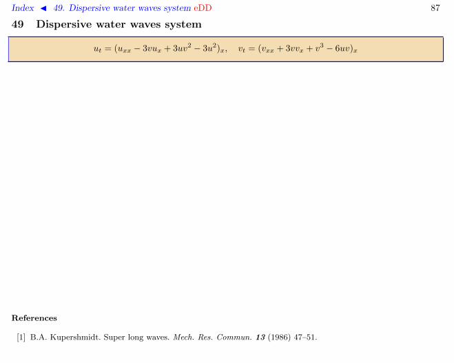
Index J 49. Dispersive water waves system eDD 87

49 Dispersive water waves system

ut = (uxx − 3vux + 3uv2 − 3u2)x, vt = (vxx + 3vvx + v3 − 6uv)x

References

[1] B.A. Kupershmidt. Super long waves. Mech. Res. Commun. 13 (1986) 47–51.

Index J 50. Dressing chain hD∆ 88

50 Dressing chain

v′n+1 + v′n = (vn+1 − vn)2 + βn

ã This differential-difference equation defines the Darboux transformation for the Schrodinger equationand x-part of the Backlund transformation for the potential KdV equation.

ã The differences fn = vn+1 − vn satisfy the equations

f ′n+1 + f ′n = f2n+1 − f2

n + βn+1 − βn (1)

which corresponds to the modified KdV equation. In this form, the dressing chain appeared in [1] as a toolfor solving quantum problems of certain types, see factorization method.

ã Zero curvature representation: L′n = Un+1Ln − LnUn, where

Un =

(vn 1

v′n − v2n − λ −vn

), Ln =

(vn+1 1

βn − vnvn+1 − λ −vn

)or

Un =

(0 1

un − λ 0

), Ln =

(fn 1

f2n + βn − λ fn

), un = 2v′n.

ã In a wide sense, the term dressing chain is applied to any differential-difference equation generated byDarboux transformations.

References

[1] L. Infeld, T.E. Hull. The factorization method. Rev. Modern Phys. 23:1 (1951) 21–68.

[2] A.P. Veselov, A.B. Shabat. Dressing chain and the spectral theory of Schrodinger operators. Funct. Anal. Appl.27:2 (1993) 81–96.

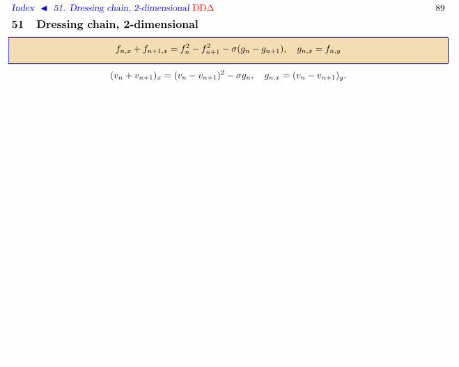
Index J 51. Dressing chain, 2-dimensional DD∆ 89

51 Dressing chain, 2-dimensional

fn,x + fn+1,x = f2n − f2

n+1 − σ(gn − gn+1), gn,x = fn,y

(vn + vn+1)x = (vn − vn+1)2 − σgn, gn,x = (vn − vn+1)y.

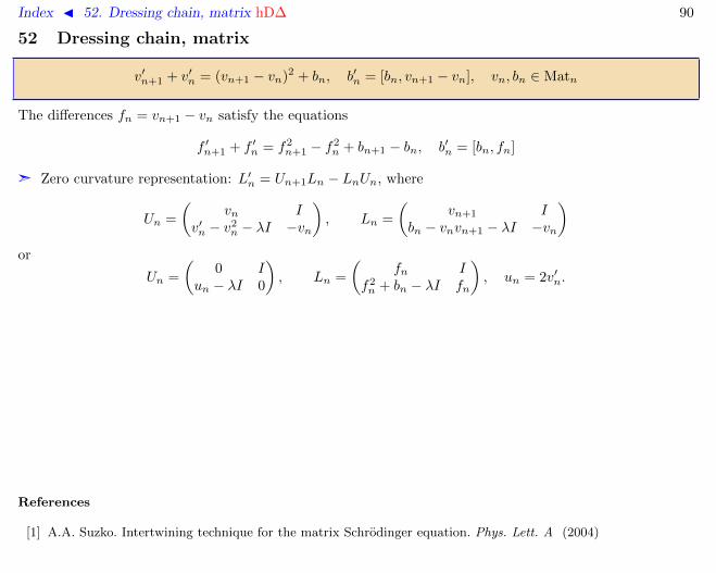
Index J 52. Dressing chain, matrix hD∆ 90

52 Dressing chain, matrix

v′n+1 + v′n = (vn+1 − vn)2 + bn, b′n = [bn, vn+1 − vn], vn, bn ∈ Matn

The differences fn = vn+1 − vn satisfy the equations

f ′n+1 + f ′n = f2n+1 − f2

n + bn+1 − bn, b′n = [bn, fn]

ã Zero curvature representation: L′n = Un+1Ln − LnUn, where

Un =

(vn I

v′n − v2n − λI −vn

), Ln =

(vn+1 I

bn − vnvn+1 − λI −vn

)or

Un =

(0 I

un − λI 0

), Ln =

(fn I

f2n + bn − λI fn

), un = 2v′n.

References

[1] A.A. Suzko. Intertwining technique for the matrix Schrodinger equation. Phys. Lett. A (2004)

Index J 53. Dressing chain, matrix twodimensional DD∆ 91

53 Dressing chain, matrix twodimensional

fn+1,x + fn,x = f2n+1 − f2

n + pn+1 − pn, pn,x = fn,t + [pn, fn].

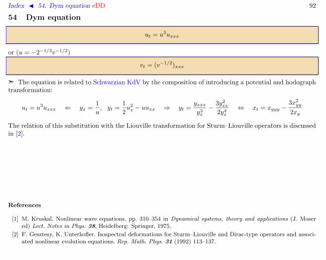
Index J 54. Dym equation eDD 92

54 Dym equation

ut = u3uxxx

or (u = −2−1/3v−1/2)

vt = (v−1/2)xxx

ã The equation is related to Schwarzian KdV by the composition of introducing a potential and hodographtransformation:

ut = u3uxxx ⇐ yx =1

u, yt =

1

2u2x − uuxx ⇒ yt =

yxxxy3x

− 3y2xx

2y4x

⇔ xt = xyyy −3x2

yy

2xy

The relation of this substitution with the Liouville transformation for Sturm–Liouville operators is discussedin [2].

References

[1] M. Kruskal. Nonlinear wave equations. pp. 310–354 in Dynamical systems, theory and applications (J. Mosered) Lect. Notes in Phys. 38, Heidelberg: Springer, 1975.

[2] F. Gesztesy, K. Unterkofler. Isospectral deformations for Sturm–Liouville and Dirac-type operators and associ-ated nonlinear evolution equations. Rep. Math. Phys. 31 (1992) 113–137.

Index J 55. Eckhaus equation eDD 93

55 Eckhaus equation

iut = uxx + 2au(|u|2)x + |a|2|u|4u

Linearizable by the substitution [1].Multifield generalizations were discussed in [2]. A discretization was proposed in [3].

References

[1] F. Calogero, S. de Lillo. The Eckhaus PDE iψt + ψxx + 2(|ψ|2)xψ + |ψ|4ψ = 0. Inverse Problems 3 (1987)633–681.

[2] F. Calogero, A. Degasperis, S. de Lillo. The multicomponent Eckhaus equation. J. Phys. A 30:16 (1997) 5805–5814.

[3] M.J. Ablowitz, C.D. Ahrens, S. de Lillo. On a “quasi” integrable discrete Eckhaus equation. J. Nonl. Math.Phys. 12:1 suppl. (2005) 1–12.

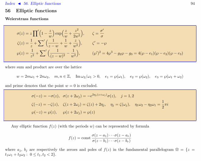
Index J 56. Elliptic functions 94

56 Elliptic functions

Weierstrass functions

σ(z) = z∏′(

1− z

w

)exp( zw

+z2

2w2

), ζ =

σ′

σ

ζ(z) =1

z+∑′ ( 1

z − w+

1

w+

z

w2

), ζ ′ = −℘

℘(z) =1

z2+∑′ ( 1

(z − w)2− 1

w2

), (℘′)2 = 4℘3 − g2℘− g3 = 4(℘− e1)(℘− e2)(℘− e3)

where sum and product are over the lattice

w = 2mω1 + 2nω2, m, n ∈ Z, Imω2/ω1 > 0, e1 = ℘(ω1), e2 = ℘(ω2), e3 = ℘(ω1 + ω2)

and prime denotes that the point w = 0 is excluded.

σ(−z) = −σ(z), σ(z + 2ωj) = −e2ηj(z+ωj)σ(z), j = 1, 2

ζ(−z) = −ζ(z), ζ(z + 2ωj) = ζ(z) + 2ηj , ηj = ζ(ωj), η1ω2 − η2ω1 =1

2πi

℘(−z) = ℘(z), ℘(z + 2ωj) = ℘(z)

Any elliptic function f(z) (with the periods w) can be represented by formula

f(z) = constσ(z − a1) · · ·σ(z − ar)σ(z − b1) · · ·σ(z − br)

where aj , bj are respectively the zeroes and poles of f(z) in the fundamental parallelogram Ω = z =t1ω1 + t2ω2 : 0 ≤ t1, t2 < 2.

Index J 56. Elliptic functions 95

Several most useful identities:

σ(x+ α)σ(x− α)σ(β + γ)σ(β − γ) = σ(x+ β)σ(x− β)σ(α+ γ)σ(α− γ)

−σ(x+ γ)σ(x− γ)σ(α+ β)σ(α− β)

ζ(x) + ζ(y) + ζ(z)− ζ(x+ y + z) =σ(x+ y)σ(y + z)σ(z + x)

σ(x)σ(y)σ(z)σ(x+ y + z)

1

2

∣∣∣∣∣∣1 ℘(x) ℘′(x)1 ℘(y) ℘′(y)1 ℘(z) ℘′(z)

∣∣∣∣∣∣ =σ(x+ y + z)σ(x− y)σ(y − z)σ(z − x)

σ3(x)σ3(y)σ3(z)

℘(x)− ℘(y) = −σ(x+ y)σ(x− y)

σ2(x)σ2(y)

1

4

(℘′(x) + ℘′(y)

℘(x)− ℘(y)

)2

= ℘(x) + ℘(y) + ℘(x− y) (1)

The biquadratic polynomial

H(u, v, w) = (uv + vw + wu+ g2/4)2 − (u+ v + w)(4uvw − g3)

satisfies the identity H2v − 2HHvv = r(u)r(w), r(u) = 4u3 − g2u− g3 (see Mobius invariants). The identity

H(℘(x), ℘(y), ℘(z)) = −σ(x+ y + z)σ(−x+ y + z)σ(x− y + z)σ(x+ y − z)σ4(x)σ4(y)σ4(z)

= (℘(x)− ℘(y))2(℘(x+ y)− ℘(z))(℘(x− y)− ℘(z))

implies the Euler form of the addition theorem (1) H(℘(x), ℘(y), ℘(x± y)) = 0.

Index J 56. Elliptic functions 96

References

[1] N.I. Akhiezer. Elements of the theory of elliptic functions. Moscow: Nauka, 1970. (in Russian)

[2] A. Hurwitz, R. Courant. Vorlesungen uber allgemeine Funktionentheorie und elliptische Funktionen. Springer-Verlag, Berlin, 1964.

Index J 57. Ermakov system D 97

57 Ermakov system

x+ ω2(t)x = x−3f(x/y), y + ω2(t)y = y−3g(x/y)

ã The case f = const was introduced in the paper [1].

ã In the general case, the system possesses the first integral

I =1

2(xy − yx)2 −

∫ x/y

z−3f(z)dz −∫ y/z

z−3g(z)dz

and is linearizable [2, 3].

References

[1] V.P. Ermakov. Second order differential equations. Integrability conditions in closed form. Izv. Kievskogo Univ.9 (1880) 1–25. [in Russian]

[2] C. Athorne. Rational Ermakov systems of Fuchsian type. J. Phys. A 24:5 (1991) 945–961.

[3] C. Athorne. Kepler–Ermakov problems. J. Phys. A 24:24 (1991) L1385–1389.

Index J 58. Ernst equation hDD 98

58 Ernst equation

Re(u)(uxx + uyy +

uxx

)= u2

x + u2y

Index J 59. Euler top D 99

59 Euler top

M = [M,Ω], M = JΩ + ΩJ, M,Ω ∈ so(d)

This ODE describes the rotation of a heavy rigid d-dimensional body around its fixed center of mass. Thecase d = 3 was solved in elliptic functions by Euler. The general case was first considered in [1] where somefirst integrals were presented. The complete set of the first integrals and the Lax representation

d

dt(M + λJ2) = [M + λJ2,Ω + λJ ]

were found in [2].

References

[1] A.S. Mischenko, Funct. Anal. Appl. 4:3 (1970) 73–78.

[2] S.V. Manakov. A remark on integration of the Euler equations for n-dimensional rigid body dynamics. Funct.Anal. Appl. 10 (1976) 328–329.

Index J 60. Euler top in quadratic potential D 100

60 Euler top in quadratic potential

M = [M,Ω] + [P, J ], P = [P,Ω], M = JΩ + ΩJ, M,Ω ∈ so(d), P = P ᵀ

This corresponds to the rotation of a d-dimensional rigid body around its fixed center of mass in the New-tonian gravitational field with an arbitrary quadratic potential. Integrability of this problem was proved in[1, 2, 3].

References

[1] A.G. Reyman. Integrable Hamiltonian systems connected with graded Lie algebras. J. Sov. Math. 19 (1982)1507–1545.

[2] O.I. Bogoyavlensky. Breaking solitons. Nonlinear integrable equations. Moscow: Nauka, 1991.

[3] O.I. Bogoyavlensky. Euler equations on finite-dimensional Lie coalgebras, arising in problems of mathematicalphysics. Russ. Math. Surveys 47 (1992) 117–189.

Index J 61. Euler top discrete ∆ 101

61 Euler top discrete

Mn+1 = W ᵀnMnWn, Mn = WnJ − JW ᵀ

n , Mn ∈ so(d), Wn ∈ SO(d)

Continuous limit: Wn = I + εΩ(εn) + o(ε2), Mn = εM(εn).

References

[1] Yu.B. Suris. The problem of integrable discretization: Hamiltonian approach. Basel: Birkhauser, 2003.

Index J 62. Euler top, discrete in quadratic potential ∆ 102

62 Euler top, discrete in quadratic potential

Mn+1 = W ᵀnMnWn + [Pn+1, JWn +W ᵀ

nJ ], Pn+1 = W ᵀnPnWn,

Mn = WnJ − JW ᵀn +

1

2(JW ᵀ

nPn − PnWnJ), Mn ∈ so(d), Wn ∈ SO(d), Pn = P ᵀn

Continuous limit: Wn = I + εΩ(εn) + o(ε2), Mn = εM(εn), Pn = ε2P (εn).

References

[1] Yu.B. Suris. The problem of integrable discretization: Hamiltonian approach. Basel: Birkhauser, 2003.

Index J 63. Euler–Darboux equation qD 103

63 Euler–Darboux equation

Author: V.G. Marikhin, 27.08.2007

uxy +αux − βuyx− y

= 0 (1)

The general “solution” is of the form

u =

∫ρ(t)(x− t)β(y − t)αdt.

The Euler–Darboux operator L = ∂x∂y + αx−y∂x −

βx−y∂y and quantum spin operators

S1 = −1

2(x2 − 1)∂x −

1

2(y2 − 1)∂y +

1

2(βx+ αy),

S2 = − i2

(x2 + 1)∂x −i

2(y2 + 1)∂y +

i

2(βx+ αy),

S3 = −x∂x − y∂y +1

2(α+ β)

generate the algebra with identities

[Sa, Sb] = iεabcSc, [S1, L] = (x+ y)L, [S2, L] = i(x+ y)L, [S3, L] = 2L

S21 + S2

2 + S23 + (x− y)2L = s(s+ 1), s =

1

2(α+ β).

Therefore Si are the Backlund operators of Euler–Darboux equation, that is if u is a solution of (1) thenui = Siu are solutions as well. For example, the seed solution u0 = (x − y)α+β+1 generates the family ofsolutions un = Pn(x, y)u0. Several first polynomials are

P1 = (α+ 1)x+ (β + 1)y, P2 = (α+ 1)(α+ 2)x2 + 2xy(α+ 1)(β + 1) + (β + 1)(β + 2)y2,

P3 = (α+ 1)(α+ 2)(α+ 3)x3 + 3(α+ 1)(α+ 2)(β + 1)x2y

+3(α+ 1)(β + 1)(β + 2)xy2 + (β + 1)(β + 2)(β + 3)y3.

Index J 64. Euler–Poisson equations D 104

64 Euler–Poisson equations

u′ = [u, Ju] + [γ, v], v′ = [v, Ju], u, v, γ ∈ R3, J = diag(J1, J2, J3), γ, J = const

The system describes the motion of a rigid body spinning around a fixed point in a uniform gravitationalfield, in three dimensions. The system is not integrable for the generic values of parameters γ, J . However,several integrable cases are known. Three quadratic integrals of motion exist for any set of parameters:

〈v, v〉 = 1, 〈u, v〉 = σ, 〈u, Ju〉 − 2〈γ, v〉 = ε.

Complete integrability requires one more first integral. It exists in the following cases:

case parameters first integral

Euler γ = 0 〈u, u〉Lagrange J1 = J2, γ1 = γ2 = 0 u3

Kowalewskaya 2J1 = 2J2 = J3, γ3 = 0 |J1(u1 + iu2)2 + 2(γ1 + iγ2)(v1 + iv2)|2

Lagrange case contains, in particular, the isotropic subcase J = id with the first integral 〈γ, u〉. Kowalevskayacase was discovered under the following setting: to find cases when the general solution of the system ismeromorphic in t. Up to the obvious changes, the above list covers all cases which satisfy this property.In contrast to the first two cases with solutions expressed in terms of elliptic functions, the solution of theKowalevskaya top is given in genus 2 hyperelliptic functions.

Several more cases are partially integrable, that is, are integrable on some invariant level set: the casesof Goryachov, Hess–Appelrot, Bobylev–Steklov and N. Kovalevski.

References

[1] S.V. Kowalevski. Sur le probleme de la rotation d’un corps solide autour d’un point fixe. Acta Math. 12 (1889)177–232.

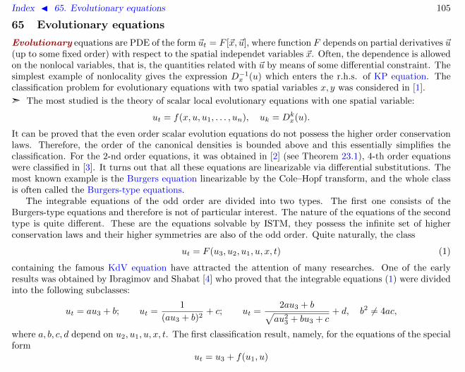
Index J 65. Evolutionary equations 105

65 Evolutionary equations

Evolutionary equations are PDE of the form ~ut = F [~x, ~u], where function F depends on partial derivatives ~u(up to some fixed order) with respect to the spatial independet variables ~x. Often, the dependence is allowedon the nonlocal variables, that is, the quantities related with ~u by means of some differential constraint. Thesimplest example of nonlocality gives the expression D−1

x (u) which enters the r.h.s. of KP equation. Theclassification problem for evolutionary equations with two spatial variables x, y was considered in [1].

ã The most studied is the theory of scalar local evolutionary equations with one spatial variable:

ut = f(x, u, u1, . . . , un), uk = Dkx(u).

It can be proved that the even order scalar evolution equations do not possess the higher order conservationlaws. Therefore, the order of the canonical densities is bounded above and this essentially simplifies theclassification. For the 2-nd order equations, it was obtained in [2] (see Theorem 23.1), 4-th order equationswere classified in [3]. It turns out that all these equations are linearizable via differential substitutions. Themost known example is the Burgers equation linearizable by the Cole–Hopf transform, and the whole classis often called the Burgers-type equations.

The integrable equations of the odd order are divided into two types. The first one consists of theBurgers-type equations and therefore is not of particular interest. The nature of the equations of the secondtype is quite different. These are the equations solvable by ISTM, they possess the infinite set of higherconservation laws and their higher symmetries are also of the odd order. Quite naturally, the class

ut = F (u3, u2, u1, u, x, t) (1)

containing the famous KdV equation have attracted the attention of many researches. One of the earlyresults was obtained by Ibragimov and Shabat [4] who proved that the integrable equations (1) were dividedinto the following subclasses:

ut = au3 + b; ut =1

(au3 + b)2+ c; ut =

2au3 + b√au2

3 + bu3 + c+ d, b2 6= 4ac,

where a, b, c, d depend on u2, u1, u, x, t. The first classification result, namely, for the equations of the specialform

ut = u3 + f(u1, u)

Index J 65. Evolutionary equations 106

was obtained in [5, 6]. The complete list of the KdV-type integrable equations with the constant separant,that is, of the form

ut = u3 + f(u2, u1, u, x) (2)

was presented in [7]. This result was an important step in the development of the symmetry approach. Thespecial quasilinear case

ut = a(u1, u, t)u3

was classified in [8]. The classification of the general case (1) was initiated in the papers [9, 10, 11, 12],however the full solution of this challenging problem is not obtained so far. Most probably, no essentiallynew equations can be found in the rest cases, accordingly to the following conjecture.

Conjecture 1 ([10]). Any integrable equation (1) is related via a contact transform or a differential substi-tution either to KdV, or to Krichever–Novikov or to the linear equation ut = u3 + a(x, t)u1 + b(x, t)u.

It is also not clear, how many higher symmetries are actually necessary for the integrability of equation(1). It may be possible that the Fokas conjecture is valid for this class of equations, that is the existence ofa single 5-th order symmetry implies the integrability.

ã The integrable equations of the 5-th order were classified only in the constant separant case [13]

ut = u5 + F (u4, u3, u2, u1, u).

These can be divided into three types: symmetries of the Burgers-type equations, symmetries of the KdV-type equations (2) and the equations without lower-order symmetries. The most known representatives ofthe latter subclass are the Kaup–Kupershmidt and Sawada–Kotera equations. The equations of this typeadmit the zero curvature representations in 3× 3 matrices, in contrast to the equations (2) for which 2× 2matrices suffice.

ã Regarding the 7-th and higher order equations only particular results are known [14, 15].

ã The two-component evolution systems of the form

~ut = A(~u)~uxx + F (~u, ~ux), ~u = (u, v)

where classified in the papers [16, 17, 18]. They are also divided into three types: equations of NLS andBoussinesq type with the zero curvature representations in 2 × 2 and 3 × 3 matrices respectively, andlinearizable equations.

Index J 65. Evolutionary equations 107

References

[1] A.V. Mikhailov, R.I. Yamilov. Towards classification of (2+1)-dimensional integrable equations. Integrabilityconditions I. J. Phys. A 31:31 (1998) 6707–6715.

[2] S.I. Svinolupov. Second-order evolution equations with symmetries. Russ. Math. Surveys 40:5 (1985) 241–242.

[3] S.I. Svinolupov. Analogues of the Burgers equations of arbitrary order. Theor. Math. Phys. 65:2 (1985) 1177–1180.

[4] N.H. Ibragimov, A.B. Shabat. On infinite dimensional Lie–Backlund algebras. Funct. Anal. Appl. 14:4 (1980)79–80.

[5] N.H. Ibragimov, A.B. Shabat. Evolutionary equations with nontrivial Lie–Backlund group. Funct. Anal. Appl.14:1 (1980) 25–36.

[6] A.S. Fokas. A symmetry approach to exactly solvable evolution equations. J. Math. Phys. 21:6 (1980) 1318–1325.

[7] S.I. Svinolupov, V.V. Sokolov. On evolution equations with nontrivial conservation laws. Funct. Anal. Appl.16:4 (1982) 86–87.

[8] L. Abellanas, A. Galindo. A Harry Dym class of bihamiltonian evolution equations. Phys. Lett. A 107:4 (1985)159–160.

[9] R. Hernandez Heredero, V.V. Sokolov, S.I. Svinolupov. Toward the classification of third order integrable evo-lution equations. J. Phys. A 27:13 (1994) 4557–4568.

[10] R. Hernandez Heredero, V.V. Sokolov, S.I. Svinolupov. Classification of third order integrable evolution equa-tions. Physica D 87:1–4 (1995) 32–36.

[11] R. Hernandez Heredero. Integrable quasilinear equations. Theor. Math. Phys. 133:2 (2002) 1514–1526.

[12] R. Hernandez Heredero. Classification of fully nonlinear integrable evolution equations of third order. J. Nonl.Math. Phys. 12:4 (2005) 567–585.

[13] A.V. Mikhailov, A.B. Shabat, V.V. Sokolov. The symmetry approach to classification of integrable equations.In: What is Integrability? (V.E. Zakharov ed). Springer-Verlag, 1991, pp. 115–184.

[14] J.A. Sanders, J.P. Wang. On the integrability of homogeneous scalar evolution equations. J. Diff. Eq. 147:2(1998) 410–434.

[15] J.A. Sanders, J.P. Wang. On the integrability of non-polynomial scalar evolution equations. J. Diff. Eq. 166:1(2000) 132–150.

[16] A.V. Mikhailov, A.B. Shabat. Integrability conditions for systems of two equations of the form ~ut = A(~u)~uxx +F (~u, ~ux). I, II. Theor. Math. Phys. 62:2 (1985) 107–122; Theor. Math. Phys. 66:1 (1986) 32–44.

Index J 65. Evolutionary equations 108

[17] A.V. Mikhailov, A.B. Shabat, R.I. Yamilov. The symmetry approach to classification of nonlinear equations.Complete lists of integrable systems. Russ. Math. Surveys 42:4 (1987) 1–63.

[18] A.V. Mikhailov, A.B. Shabat, R.I. Yamilov. Extension of the module of invertible transformations. Classificationof integrable systems. Commun. Math. Phys. 115:1 (1988) 1–19.

Index J 66. Equivalence problem 109

66 Equivalence problem

The equivalence problem consists of finding the necessary and sufficient conditions which allow to determinewhether two equations of the class under consideration are equivalent modulo some set of transformations,and in the effective construction of such transformation if it exists. As usual, the admissible transformationsare assumed to be the point or contact ones or their subgroups preserving the general form of equationsunder scrutiny; sometimes differential substitutions are allowed as well.

The importance of this problem is explained by the fact that the differential equations are not an invariantobject and therefore the study of transformations must be an essential part of the general theory.

The classical work [4] demonstrates the complexity of such sort of the problems even in the simplest caseof second order ODE.

References

[1] L.V. Ovsyannikov. Group analysis of differential equations, New York: Academic Press, 1982.

[2] N.H. Ibragimov. Transformation groups applied to mathematical physics. Dordrecht: Reidel, 1985.

[3] P.J. Olver. Applications of Lie groups to differential equations, 2nd ed., Graduate Texts in Math. 107, NewYork: Springer-Verlag, 1993.

[4] M.A. Tresse. Determination des invariants ponctuels de l’equation differentielle ordinaire du second ordre y′′ =w(x, y, y′). Leipzig: Hirzel, 1896.

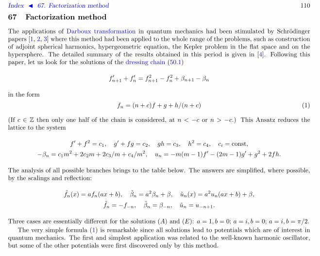
Index J 67. Factorization method 110

67 Factorization method

The applications of Darboux transformation in quantum mechanics had been stimulated by Schrodingerpapers [1, 2, 3] where this method had been applied to the whole range of the problems, such as constructionof adjoint spherical harmonics, hypergeometric equation, the Kepler problem in the flat space and on thehypersphere. The detailed summary of the results obtained in this period is given in [4]. Following thispaper, let us look for the solutions of the dressing chain (50.1)

f ′n+1 + f ′n = f2n+1 − f2

n + βn+1 − βn

in the form

fn = (n+ c)f + g + h/(n+ c) (1)

(If c ∈ Z then only one half of the chain is considered, at n < −c or n > −c.) This Ansatz reduces thelattice to the system

f ′ + f2 = c1, g′ + fg = c2, gh = c3, h2 = c4, ci = const,

−βn = c1m2 + 2c2m+ 2c3/m+ c4/m

2, un = −m(m− 1)f ′ − (2m− 1)g′ + g2 + 2fh.

The analysis of all possible branches brings to the table below. The answers are simplified, where possible,by the scalings and reflection:

fn(x) = afn(ax+ b), βn = a2βn + β, un(x) = a2un(ax+ b) + β,

fn = −f−n, βn = β−n, un = u−n+1.

Three cases are essentially different for the solutions (A) and (E): a = 1, b = 0; a = i, b = 0; a = i, b = π/2.

The very simple formula (1) is remarkable since all solutions lead to potentials which are of interest inquantum mechanics. The first and simplest application was related to the well-known harmonic oscillator,but some of the other potentials were first discovered only by this method.

Index J 67. Factorization method 111

The abridged classification of factorization types accordingly to Infeld and Hull

fn βn un

(A) am cot(ax+ b) +d

sin(ax+ b)a2m2 1

sin2(ax+ b)(a2m(m− 1) + d2 [5]

+ad(2m− 1) cos(ax+ b))

(B) ex −m −m2 e2x − (2m− 1)ex [6]

(C)m

x+ dx −d(4m+ 1)

m(m− 1)

x2− 2dm+ d2x2

(D) −x 2n+ 1 x2 + 2n

(E) am cot(ax+ b) +d

ma2m2 − d2/m2 m(m− 1)

a2

sin2(ax+ b)[7, 8]

+2ad cot(ax+ b)

(F )m

x+d

m−d2/m2 m(m− 1)

x2+

2d

x

References

[1] E. Schrodinger. A method of determining quantum-mechanical eigenvalues and eigenfunctions. Proc. Roy. IrishAcad. A 46 (1940) 9–16.

[2] E. Schrodinger. Further studies on solving eigenvalue problems by factorization. Proc. Roy. Irish Acad. A 46(1941) 183–206.

[3] E. Schrodinger. The factorization of hypergeometric equation. Proc. Roy. Irish Acad. A 47 (1941) 53–54.

[4] L. Infeld, T.E. Hull. The factorization method. Rev. Modern Phys. 23:1 (1951) 21–68.

Index J 67. Factorization method 112

[5] G. Poschl, E. Teller. Bemerkungen zur Quantenmechanik des anharmonischen Oszillators. Zeits. Physik 83:3-4(1933) 143–151.

[6] P.M. Morse. Diatomic molecules according to the wave mechanics. II. Vibrational levels. Phys. Rev. 34:1 (1929)57–64.

[7] M.F. Manning. Exact solutions of the Schrodinger equation. Phys. Rev. 48:2 (1935) 161–164.

[8] N. Rosen, P.M. Morse. On the vibrations of polyatomic molecules. Phys. Rev. 42:2 (1932) 210–217.

Index J 68. Fermi–Pasta–Ulam–Tsingou lattice eD∆ 113

68 Fermi–Pasta–Ulam–Tsingou lattice

Author: V.E. Adler, 26.12.2008

ω−2un,tt = un+1 − 2un + un−1 + a(un+1 − un)2 − a(un − un−1)2 (1)

The system describes an one-dimensional lattice of anharmonic oscillators. Its numeric investigation wasundertaken in the paper [1]. It was expected that the nonlinear interaction would result quickly in an uniformdistribution of the energy over all modes, in accordance with Debye theory [2], however it turned out thatthe energy transport occured only between few lower modes. Due to the periodic boundary conditionsun = un+N the recurrence of initial states was observed. (The capacity of MANIAC-I, the first computerin the world, which was used in this first numerical experiment in mathematical physics allowed to takeN = 64.) A qualitative explanation of recurrence phenomena was proposed in [3] on the base of the notionof solitons, that is the nonlinear travelling waves which interact elastically with each other. More precisely,this notion was introduced not for the lattice (1), but for Korteweg-de Vries equation which is its continuouslimit. In turn, KdV equation was replaced, in the numeric study, by the difference equation

uj+1n = uj−1

n − k

3h(ujn+1 + ujn + ujn−1)(ujn+1 − u

jn−1)− δ2k

h3(ujn+2 − 2ujn+1 + 2ujn−1 − u

jn+2)

with the periodicity condition ujn = ujn+2N . It should be stressed that both this discretization and the lattice(1) itself are not integrable, so that, strictly speaking, the waves in both numerical experiments demonstratedonly soliton-like behavior. Nevertheless, the further studies lead to the development of the exact theory ofsoliton solutions and to discovery of the integration method of KdV by means of the inverse scatteringproblem. The complete explanation of the recurrence phenomenon was obtained after development of thetheory of finite-gap solutions (the soliton solutions correspond to the limit N →∞).

ã The continuous limit for the lattice (1): let un(t) = u(x, τ), x = nh, τ = ωht, then Taylor expansion ofun±1 is

un±1 = u± hux +h2

2uxx ±

h3

6uxxx +

h4

24uxxxx + o(h5), h→ 0,

Index J 68. Fermi–Pasta–Ulam–Tsingou lattice eD∆ 114

and one comes to the Boussinesq-type approximation

uττ = uxx + 2ahuxuxx +h2

12uxxxx + o(h3),

which describes the wave propagation in both directions. Next, assume that the parameter a is althoughsmall, a = κh. Then the change u(x, τ) = v(X,T ), X = x+ τ , T = κh2τ , 24κ = δ−1 brings to

VXT = VXVXX + δVXXXX + o(h),

that is the KdV equation for VX .

ã The detailed discussion of FPU experiment is given in the books [4, 5, 6]. The preprint [1] was reprintedin number of sources, their list and some interesting, but not well-known historical facts can be found in [7].In should be mentioned that a lattice, analogous to (1) was proposed earlier in the paper [8].

References

[1] E. Fermi, J. Pasta, S. Ulam. Studies of nonlinear problems. I. Los Alamos report LA-1940 (1955).

[2] P. Debye. Vortrage uber der kinetische Theorie die Materie und der Elektrizitat. Leipzig, 1914.

[3] N.J. Zabusky, M.D. Kruskal. Interaction of “solitons” in a collisionless plasma and the recurrence of initialstates. Phys. Rev. Let. 15:6 (1965) 240–243.

[4] M.J. Ablowitz, H. Segur. Solitons and the Inverse Scattering Transform. Philadelphia: SIAM, 1981.

[5] R.K. Dodd, J.C. Eilbeck, J.D. Gibbon, H.C. Morris. Solitons and nonlinear wave equations. London: AcademicPress, 1982.

[6] A.C. Newell. Solitons in mathematics and physics. Philadelphia: SIAM, 1985.

[7] T. Dauxois. Fermi, Pasta, Ulam and a mysterious lady. arXiv:0801.1590v1

[8] T.A. Kontorova, Ya.I. Frenkel. JETP 8 (1938) 89.

Index J 69. Fischer equation eDD 115

69 Fischer equation

ut = uxx + u− u2

ã Applications in biology and chemical kinetics.

ã Not integrable [3, 4]. Some exact solutions are found in [5].

ã See also: Burgers–Huxley, Kolmogorov–Petrovsky–Piskunov equations.

References

[1] R.A. Fischer. The wave of advance of an advantageous gene. Ann. Eugen. 7 (1937) 355–369.

[2] F. Hoppenstaedt. Mathematical theories of populations: demographics, genetics and epidemics. CBMS RegionalConference Series in Appl. Math. 20 (1975) SIAM, Philadelphia.

[3] M.J. Ablowitz, H. Segur. Solitons and the Inverse Scattering Transform. Philadelphia: SIAM, 1981.

[4] M.J. Ablowitz, A. Zeppetella. Explicit solutions of Fischer’s equation for a special wave speed. Bull. Math. Biol.41:6 (1979) 835–840.

[5] N.A. Kudryashov. On exact solutions of families of Fischer equations. Theor. Math. Phys. 94:2 (1993) 211–218.

Index J 70. Fornberg–Whitham equation DD 116

70 Fornberg–Whitham equation

ut − uxxt + ux = uuxxx + 3uxuxx − uux

References

[1] B. Fornberg, G.B. Whitham. A numerical and theoretical study of certain nonlinear wave phenomena. Phil.Trans. R. Soc. London A 289 (1978) 373–404.

[2] G.B. Whitham. Proc. R. Soc. A 299 (1967) 6–25.

[3] G.B. Whitham. Linear and nonlinear waves, N.Y.: Wiley, 1974.

[4] C.R. Gilson, A. Pickering. Factorization and Painleve analysis of a class of nonlinear third-order partial differ-ential equations. J. Phys. A 28:10 (1995) 2871–2888.

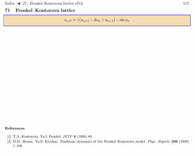
Index J 71. Frenkel–Kontorova lattice eD∆ 117

71 Frenkel–Kontorova lattice

un,tt = γ(un+1 − 2un + un−1)− sinun

References

[1] T.A. Kontorova, Ya.I. Frenkel. JETP 8 (1938) 89.

[2] O.M. Braun, Yu.S. Kivshar. Nonlinear dynamics of the Frenkel–Kontorova model. Phys. Reports 306 (1998)1–108.

Index J 72. Garnier system D 118

72 Garnier system

u′′ = 〈u, v〉u+ Ju, v′′ = 〈u, v〉v + Jv, u, v ∈ Rd, J = diag(J1, . . . , Jd)

Index J 73. Garnier system discrete ∆ 119

73 Garnier system discrete

〈un+1, un〉un+1 + 〈un, un〉un + 〈un, un−1〉un−1 = Jun, un ∈ Rd, J = diag(J1, . . . , Jd)

-10 -5 0 5 10

-10

-5

0

5

10

Index J 74. Gauge transformations 120

74 Gauge transformations

Example 1. The Liouville transformation

dx = r2dy, ψ = rφ, u = q/r4 + rxx/r

relates two forms of Sturm–Liouville equation:

ψxx = (u(x)− λ)ψ ↔ φyy = (q(y)− λr4(y))φ.

In particular, the choice r = ψ(x, 0) brings to another canonical form (so called acoustic spectral problem)

φyy = −λr4(y)φ. (1)

For this, the Darboux transformation (37.1) is gauge invariant to the following one [1]:

φ = φy/p− φ, p := φ(α)y /φ(α), py + p2 = −αr4, r = p/r, r2dy = r2dy.

References

[1] V.E. Adler, A.B. Shabat. Dressing chain for the acoustic spectral problem. Theor. Math. Phys. 149:1 (2006)1324–1337.

Index J 75. Gerdjikov–Ivanov equation eDD 121

75 Gerdjikov–Ivanov equation

iut = uxx − iu2ux +1

2u3u2

Alias: DNLS-III equation

References

[1] V.S. Gerdjikov, M.I. Ivanov. Bulg. J. Phys. 10 (1983) 130.

[2] A. Kundu. Exact solutions to higher-order nonlinear equations through gauge transformation. Physica D 25:1-3(1987) 399–406.

[3] E. Fan. Darboux transformation and soliton-like solutions for the Gerdjikov–Ivanov equation. J. Phys. A 33:39(2000) 6925–6933.

Index J 76. Hamiltonian structure 122

76 Hamiltonian structure

Author: A.Ya. Maltsev, 2.10.2009

1. Finite-dimensional dynamical systems2. Discrete infinite-dimensional Poisson brackets3. Evolutionary PDEs4. Poisson brackets of hydrodynamic type5. Weakly nonlocal Poisson brackets and symplectic structures

General references: [1, 2, 3, 4, 5]

1. Finite-dimensional dynamical systems

A Poisson bracket on a finite-dimensional manifold Mn with local coordinates x = (x1, . . . , xn) is givenby a contravariant 2-tensor J ij(x) which is skew-symmetric

J ij(x) = −Jji(x) (1)

and satisfies the Jacobi identity

J iq∂Jjk

∂xq+ Jjq

∂Jki

∂xq+ Jkq

∂J ij

∂xq= 0 (2)

(summation over repeated indices is assumed everywhere). The Poisson bracket of two smooth functionsf(x), g(x) on Mn is given then by the formula

f, g =∂f

∂xiJ ij

∂g

∂xj.

It is easy to see that xi, xj = J ij(x).The following identities take place on the space of smooth functions on Mn:

bilinearity αf + βg, h = αf, h+ βg, h,

Index J 76. Hamiltonian structure 123

skew-symmetry f, g = −g, f,Leibnitz identity fh, g = fh, g+ hf, g,Jacobi identity f, g, h+ g, h, f+ h, f, g = 0.

Thus, a Poisson bracket gives a structure of Lie algebra on the space of smooth functions on Mn. ThePoisson bracket on Mn is called also a Poisson structure on Mn and the manifold Mn is called aPoisson manifold in this case.

A Poisson bracket onMn is called non-degenerate if det ||J ij || 6= 0 everywhere onMn. A non-degeneratePoisson bracket can exist only on even-dimensional manifolds Mn, such that n = 2m, m ∈ N.

A function N(x) such thatN, f ≡ 0

for any smooth function f on Mn is called annihilator or Casimir function of the Poisson bracket onMn. It is easy to see that every Casimir function should satisfy in local coordinates the equation

J ij∂N

∂xj≡ 0.

A Poisson bracket has constant rank l = 2s on Mn if rank ||J ij || = l everywhere on Mn. In this caselocally there always exist exactly n− l independent functions (N1(x), . . . , Nn−l(x)) which give a set of localCasimir functions for the corresponding chart of Mn.

The common level surfaces of the local Casimir functions

N1(x) = const, . . . , Nn−l(x) = const

represent an integrable foliation which is uniquely globally defined on the manifoldMn. However, this doesnot mean necessarily that the functions (N1, . . . , Nn−l) can be globally defined on the manifold Mn, sincethe choice of independent set (N1(x), . . . , Nn−l(x)) is individual for every local chart of Mn. Thus, it isnot possible to state in general that a Poisson bracket of constant rank l on Mn has n− l globally definedCasimir functions on this manifold. This means certainly, that the corresponding foliation given by a Poissonstructure of constant rank in general can not be defined as a set of common level surfaces of a set of globalfunctions (N1, . . . , Nn−l) on Mn.

Index J 76. Hamiltonian structure 124

The important fact is that in general even the gradients of Casimir functions can not be globally definedonMn as a set of global closed 1-forms onMn. As a result, the foliations defined by the Casimir functionsof a Poisson structure on a manifold can in general be topologically more complicated than the foliationsdefined by a set of closed 1-forms on Mn.

For non-degenerate Poisson structure on Mn the form

ωij = ||J ij ||−1

can be defined everywhere on Mn. For any non-degenerate Poisson structure on Mn the form ωij is aglobally defined non-degenerate closed 2-form onMn. The manifoldMn is called in this case a symplecticmanifold and the form ωij gives the symplectic form of Mn. Vice versa, on every symplectic manifoldMn the non-degenerate Poisson structure can be defined.

Every smooth function f on a Poisson manifoldMn generates a smooth vector field ξf according to theformula

ξif (x) = J ij(x)∂f

∂xj.

The vector field ξf (x) is called the Hamiltonian vector field generated by f and the function f is calledits Hamiltonian function. The vector field ξ(x) is called locally Hamiltonian if in the vicinity of everypoint x0 ∈ Mn there exists a local function f(x) which gives locally a Hamiltonian function for the fieldξ(x).

Every locally Hamiltonian vector on Mn generates a one-parametric group of transformations of Mn

which preserves the Poisson structure on Mn. The last statement follows immediately from the fact thatthe Lie derivative of the tensor J ij along the vector field ξ vanishes identically in this case.

The remarkable fact, which follows from the Jacobi identity for J ij on Mn, is that the mapping

f → ξf

defines the homomorphism of Lie algebras from the Lie algebra of functions to the Lie algebra of the vectorfields on Mn. So the vector field

[ξf , ξg]i = ξjf

∂ξig∂xj− ξjg

∂ξif∂xj

Index J 76. Hamiltonian structure 125

is a Hamiltonian vector field with the Hamiltonian function h = f, g.The analogous statement is true also for locally Hamiltonian vector fields. Thus, both Hamiltonian and

locally Hamiltonian vector fields onMn give the sub-algebras in the Lie algebra of the vector fields onMn.The Poisson bracket of two functions f, g has a very important meaning. Namely, it gives the derivative

of the function f along the vector field ξg generated by g. In particular, the function f gives a conservationlaws for the dynamical system corresponding to ξg if and only if f, g ≡ 0 everywhere on Mn. It is easyto see then that the function g always gives the conservation law for ξg which represents the conservation ofenergy for the Hamiltonian vector field.

It is not difficult to show by use of Jacobi identity that the Poisson bracket of any two conservationlaws for the vector field ξ(x) gives also a conservation law for the same vector field. So, the conservationlaws for the Hamiltonian vector field ξ(x) generated by any function g(x) on Mn represent always the Liesub-algebra in the Lie algebra of functions on Mn.

The canonical form of the non-degenerate Poisson bracket on a manifold Mn = M2m is given by thefollowing theorem.

Theorem 1 (Darboux). For any non-degenerate Poisson bracket on the manifold M2m there exist locallythe coordinates (q1, . . . , qm, p1, . . . , pm) such that

qα, qβ = 0, pα, pβ = 0, qα, pβ = δαβ , α, β = 1, . . . ,m

where δαβ is the Kronecker symbol.

Darboux theorem can be generalized also to the case of constant rank Poisson brackets by use of thelocally defined Casimir functions.

Theorem 2. For any Poisson bracket of constant rank l = 2s on a manifoldMn there exist local coordinates(N1, . . . , Nn−2s, q1, . . . , qs, p1, . . . , ps) such that

Nλ, Nµ = 0, Nλ, qα = 0, Nλ, pα = 0,

qα, qβ = 0, pα, pβ = 0, qα, pβ = δαβ ,

where λ, µ = 1, . . . , N − 2s and α, β = 1, . . . , s.

Index J 76. Hamiltonian structure 126

It is easy to see that the coordinates (N1, . . . , Nn−2s) play the role of local Casimir functions in thiscase. The Poisson bracket of the functions (q1, . . . , qs, p1, . . . , ps) gives a non-degenerate Poisson bracket onevery surface N1 = const, . . . , Nn−2s = const. This bracket is called a restriction of the Poisson bracket ofconstant rank to the common level surfaces of Casimir functions.

The non-degenerate Poisson brackets in the canonical form are closely connected with the Lagrangianapproach in classical mechanics. Let q = (q1, . . . , qm) be the generalized coordinates of a mechanical systemand K and Π be, respectively, its kinetic and potential energy. Then the famous Lagrangian functional

S =

∫ t2

t1

L(q, q) dt =

∫ t2

t1

(K(q, q)−Π(q)) dt

leads to the non-degenerated Poisson structure through the Legendre transformation. Namely, as is wellknown, the Lagrangian equations

d

dt

∂L

∂qi− ∂L

∂qi= 0, i = 1, . . . , s

are equivalent to the equations

qi =∂H(q,p)

∂pi, pi = −∂H(q,p)

∂qi

after the transformation

pi =∂L

∂qi, H(q,p) ≡ L(q, q(q,p))− qi(q,p)

∂L

∂qi(q, q(q,p))

The transformation from the Lagrangian formalism to non-degenerate Hamiltonian formalism can be madealso in more general case of Lagrangian functions depending on higher derivatives of the coordinates q byuse of Ostrogradskii transformations.

Example 3. Lie–Poisson bracket. The most important examples of the Poisson brackets of constant rankare given by the Poisson brackets defined by the Lie algebras. Namely, if L is a Lie algebra with a basic(e1, . . . , en) and the structure constants Cijk

[ej , ek] = Cijkei

Index J 76. Hamiltonian structure 127

(summation over repeated indices), then the natural Poisson bracket on the dual space L∗ with coordinates(x1, . . . , xn) can be defined as

xj , xk = Cijkxi.

The Casimir functions of the universal enveloping algebra play then the role of the natural annihilators ofthis Poisson bracket.

The Hamiltonian formulation plays an important role in the definition of complete integrability of dy-namical system, see Liouville integrability. In particular, the nice construction underlying the integrabilityin many important examples is the bi-Hamiltonian structure.

2. Discrete infinite-dimensional Poisson brackets

The infinite-dimensional Poisson brackets are the generalizations of the finite-dimensional Poisson bracketswhere the number of coordinates is infinite. The same properties of the skew-symmetry and Jacobi identityare also required in the infinite-dimensional case. As a rule, the infinite-dimensional Poisson brackets ariseas the field-theoretical (discrete or continuous) Poisson brackets for the field-theoretical systems or PDE’s.As an example, let us consider the infinite-dimensional discrete Poisson bracket on the space of fields ϕ(k) =(ϕ1(k), . . . , ϕn(k)) where k is the integer number k ∈ Z numerating the positions of cells in the case of onespatial dimension.

The values ϕ(k) play now the role of “coordinates” in the functional space and the general form of thePoisson bracket can be written as

ϕi(k), ϕj(l) = J ijkl [ϕ] (3)

where J ijkl [ϕ] are some functionals on the functional space ϕ(k).In most of important cases all functionals J ijkl [ϕ] depend just on the finite number of field variables ϕ(k′)

such that the Jacobi identity has a normal form (2).

Bracket (3) is called local if

J ijkl ≡ 0, |k − l| > N1,∂J ijkl

∂ϕq(m)≡ 0, |k −m| > N2

Index J 76. Hamiltonian structure 128

for some N1, N2. Bracket (3) is called translational invariant if it is invariant under all (integral) shifts ofthe field index k: ϕi(k)→ ϕi(k + k0).

The general form of a dynamical system generated by a functional H = H[ϕ] can be written in a naturalway

ϕi(k) =∑j,l

J ijkl [ϕ]∂H

∂ϕj(l).

The functional H[ϕ] is usually called local functional if it is of the form

H[ϕ] =

∞∑k=−∞

hk[ϕ]

where∂hk∂ϕi(l)

≡ 0, |k − l| > N

for some N > 0. In the same way, the functional H[ϕ] is called translational invariant functional if it isinvariant under the integral shifts ϕi(k)→ ϕi(k + k0).

The local translational invariant brackets (3) play very important role in the theory of one-dimensionaldiscrete dynamical systems both in integrable and non-integrable cases. It is easy to see also how thedefinitions above can be generalized to the case of several spatial variables.

3. Local field-theoretical Poisson brackets and symplectic structures

The continuous version of the infinite-dimensional Poisson brackets can be defined on the space of smoothfunctions ϕ(x) = (ϕ1(k), . . . , ϕn(x)), x ∈ R. The values ϕ(x) can be considered then as the “coordinates”on this functional space and the general form of the infinite-dimensional Poisson bracket can be written as

ϕi(x), ϕj(y) = J ij [ϕ](x, y) (4)

where J ij(x, y) are some distributions on R× R.

Index J 76. Hamiltonian structure 129

The skew-symmetry properties and the Jacobi identity

ϕi(x), ϕj(y), ϕk(z)+ ϕj(y), ϕk(z), ϕi(x)+ ϕk(z), ϕi(x), ϕj(y) = 0

are required in the sense of distributions in this case.As a rule, brackets (4) are considered on the space of rapidly decreasing or periodic functions ϕ(x).The functional I[ϕ] is called here the smooth functional if the variational derivatives δI/δϕi(x) are the

smooth functions of x. The Poisson bracket of the smooth functionals can be formally written as

I, J =

∫ +∞

−∞

∫ +∞

−∞

δI

δϕi(x)J ij [ϕ](x, y)

δJ

δϕj(y)dx dy ≡ Jij [ϕ]

(δI

δϕi(x)⊗ δJ

δϕj(y)

)where Jij is a functional corresponding to the distribution J ij(x, y).

Poisson bracket (4) is called local if it is of the form

ϕi(x), ϕj(y) =∑k≥0

Bij(k)(ϕ,ϕx, . . . )δ(k)(x− y) (5)

where Bij(k)(ϕ,ϕx, . . . ) are some smooth functions of (ϕ,ϕx, . . . ) and δ(k)(x − y) ≡ ∂k/∂xkδ(x − y). It is

assumed also that all Bij(k) depend on the finite number of arguments and the sum contains just the finite

number of terms.The corresponding Hamiltonian operator J ij can be written in this case as

J ij =∑k≥0

Bij(k)(ϕ,ϕx, . . . )∂k

∂xk

and the Poisson bracket of two smooth functionals I, J can be written then in the form

I, J =

∫ +∞

−∞

δI

δϕi(x)

∑k≥0

Bij(k)(ϕ,ϕx, . . . )∂k

∂xkδJ

δϕj(x)dx

Index J 76. Hamiltonian structure 130

The general form of dynamical system generated by the “local” functional H

H =

∫ +∞

−∞h(ϕ,ϕx, . . . ) dx

can be represented as

ϕi =∑k≥0

Bij(k)(ϕ,ϕx, . . . )∂k

∂xkδH

δϕj(x)

and gives a local expression for the “vector field” ξi(x) generated by H.Brackets (5) play an important role both for integrable and non-integrable evolution systems, however,

the complete theory of these brackets is still absent at the moment.Another important object is the local symplectic form on the space of fields ϕi(x) having the form

Ωij(x, y) =∑k≥0

ω(k)ij (ϕ,ϕx, . . . ) δ

(k)(x− y). (6)

The corresponding symplectic operator can be written as

Ωij =∑k≥0

ω(k)ij (ϕ,ϕx, . . . )

∂k

∂xk

and the connection between the time-derivative of ϕi(x) and Hamiltonian functional H is given by∑k≥0

ω(k)ij (ϕ,ϕx, . . . )

∂k

∂xkϕj =

δH

δϕi(x).

Symplectic form (6) should satisfy the skew-symmetry and closeness conditions on the space of functionsϕi(x):

Ωij(x, y) = −Ωji(y, x),δΩij(x, y)

δϕk(z)+δΩjk(y, z)

δϕi(x)+δΩki(z, x)

δϕj(y)= 0.

Index J 76. Hamiltonian structure 131

4. Poisson brackets of hydrodynamic type

An important class of local field-theoretical Poisson brackets is given by the local Poisson brackets of hy-drodynamic type, or Dubrovin–Novikov brackets [6, 7].

Definition 4. The Dubrovin–Novikov bracket (DN-bracket) is a bracket on the functional space (U1(x), . . . , UN (x))of the form

Uν(x), Uµ(y) = gνµ(U)δ′(x− y) + bνµλ (U)Uλx δ(x− y). (7)

The bracket (7) is called non-degenerate if det ||gνµ(U)|| 6= 0.

The corresponding Hamiltonian operator Jνµ can be written as

Jνµ = gνµ(U)∂

∂x+ bνµλ (U)Uλx

and is homogeneous w.r.t. transformation x→ ax.Every functional H of hydrodynamic type, that is the functional of the form

H =

∫ +∞

−∞h(U)dx

generates a system of hydrodynamic type according to the formula

Uνt = JνµδH

δUµ(x)= gνµ(U)

∂

∂x

∂h

∂Uµ+ bνµλ (U)

∂h

∂UµUλx . (8)

It was shown by Dubrovin and Novikov themselves that the theory of DN-brackets is closely connectedwith Riemannian geometry. In fact, it follows from the skew-symmetry of (7) that the coefficients gνµ(U)give in the non-degenerate case the contravariant pseudo-Riemannian metric on the manifold MN withcoordinates (U1, . . . , UN ) while the functions

Γνµλ(U) = −gµα(U)bανλ (U)

Index J 76. Hamiltonian structure 132

(where gνµ(U) is the corresponding metric with lower indices) give the connection coefficients compatiblewith metric gνµ(U). The validity of Jacobi identity requires then that gνµ(U) is actually a flat metric onthe manifold MN and the functions Γνµλ(U) give a symmetric (Levi–Civita) connection on MN .

In the flat coordinates n1(U), . . . , nN (U) the non-degenerate DN-bracket can be written in constantform:

nν(x), nµ(y) = eνδνµδ′(x− y), eν = ±1.

The functionals

Nν =

∫ +∞

−∞nν(x) dx

are the annihilators of the bracket (7) and the functional

P =1

2

∫ +∞

−∞

N∑ν=1

eν(nν(x))2 dx

is the momentum functional generating the system Uνt = Uνx according to (8).Another important choice of coordinates for DN-bracket is given by the so-called “physical” or “Liouville”

coordinates. This type of coordinates is usually associated with the densities of conservation laws of thehydrodynamic systems. We say that the coordinates are “Liouville” or “physical” for the DN-bracket if thebracket has the form:

Uν(X), Uµ(Y ) = (γνµ(U) + γµν(U))δ′(X − Y ) +∂γνµ

∂UλUλXδ(X − Y )

for some functions γνµ(U). Any coordinates such that integrals of them define the commuting flows, arephysical in that sense.

Let us mention also that the degenerate brackets (7) are more complicated but have a nice differentialgeometric structure as well.

The brackets (7) are closely connected with the integration theory of systems of hydrodynamic type

Uνt = V νµ (U)Uµx . (9)

Index J 76. Hamiltonian structure 133

Namely, according to conjecture of S.P. Novikov, all diagonalizable systems (9) which are Hamiltonian withrespect to DN-brackets (7) (with Hamiltonian function of hydrodynamic type) are completely integrable.This conjecture was proved by S.P. Tsarev who proposed a general procedure called generalized hodographmethod of integration of Hamiltonian diagonalizable systems (9).

In fact the generalized hodograph method permits to integrate the wider class of diagonalizable sys-tems (9) (semi-Hamiltonian systems) which appeared to be Hamiltonian in more general (weakly nonlocal)Hamiltonian formalism.

The symplectic structure corresponding to non-degenerate DN-bracket has the “weakly nonlocal” formand can be written in coordinates nν as

Ωνµ(x, y) = eνδνµσ(x− y), σ(x− y) = 1/2 sign(x− y).

More generally, in arbitrary coordinates Uν one has

Ωνµ(x, y) =

N∑λ=1

eλ∂nλ

∂Uν(x)σ(x− y)

∂nλ

∂Uµ(y).

5. Weakly nonlocal Poisson brackets and symplectic structures

The field-theoretical Poisson bracket is called weakly nonlocal [8] if it can be written in the form

ϕi(x), ϕj(y) =∑k≥0

Bijk (ϕ,ϕx, . . . )δ(k)(x− y) +

∑k≥0

ekSi(k)(ϕ,ϕx, . . . )σ(x− y)Sj(k)(ϕ,ϕy, . . . ) (10)

where ek = ±1, σ(x − y) = −σ(y − x), ∂xσ(x − y) = δ(x − y) and both sums contain the finite numbersof terms depending on the finite numbers of derivatives of ϕ with respect to x. It is assumed also that the“vector-fields”

S(s)(ϕ,ϕx, . . . ) =(S1

(s)(ϕ,ϕx, . . . ), . . . Sn(s)(ϕ,ϕx, . . . )

)tare linearly independent (over constant coefficients).

Index J 76. Hamiltonian structure 134

We can introduce also the Hamiltonian operator J ij :

J ij =∑k≥0

Bij(k)(ϕ,ϕx, . . . )∂k

∂xk+

g∑s=1

esSi(s)(ϕ,ϕx, . . . )D

−1Sj(s)(ϕ,ϕx, . . . ) (11)

where D−1 is the integration operator defined in the skew-symmetric way:

D−1ξ(x) =1

2

∫ x

−∞ξ(y)dy − 1

2

∫ +∞

x

ξ(y)dy.

For the functional H[ϕ] the corresponding dynamical system can be written in the form:

ϕit = J ijδH

δϕj(x)=∑k≥0

Bij(k)(ϕ,ϕx, . . . )∂k

∂xkδH

δϕj(x)

+

g∑s=1

esSi(s)(ϕ,ϕx, . . . )D

−1[Sj(s)(ϕ,ϕx, . . . )

δH

δϕj(x)

]. (12)

As previously, operator (11) should also be skew-symmetric and satisfy the Jacobi identity.It is not difficult to see that the functional

H =

∫ +∞

−∞h(ϕ,ϕx, . . . )dx (13)

generates a local dynamical systemϕit = Si(ϕ,ϕx, . . . )

according to (12) if it gives a conservation law for all the dynamical systems

ϕits = Si(s)(ϕ,ϕx, . . . )

that ishts ≡ ∂xQs(ϕ,ϕx, . . . )

Index J 76. Hamiltonian structure 135

for some functions Qs(ϕ,ϕx, . . . ).Let us formulate the result which relates the non-local and local parts of the general weakly-nonlocal

Poisson brackets (10).

Theorem 5 ([9]). For any bracket (10) the flows

ϕits = Si(s)(ϕ,ϕx, . . . ) (14)

commute with each other and leave the bracket (10) invariant.

It can be easily proved also that the flows (14) commute with any local Hamiltonian flow in the structure(10) generated by local Hamiltonian functional (13).

The general weakly nonlocal Poisson bracket of hydrodynamic type (Ferapontov bracket) has the form(ek = ±1)

Uν(x), Uµ(y) = gνµ(U)δ′(x− y) + bνµλ (U)Uλx δ(x− y) +

g∑k=1

ekwν(k)λ(U)Uλx σ(x− y)wµ(k)δ(U)Uδy . (15)

The statements analogous to the local situation can be proved also in the case of the bracket (15).

Theorem 6 ([10]). The bracket (15) satisfies the Jacobi Identity if and only if the values Γνµλ = −gµαbανλgive the Cristofel connection for the metric gνµ and the metric gνµ (with lower indices) and tensors wν(k)µ

satisfy the equations:

gντwτ(k)µ = gµτw

τ(k)ν , ∇νwµ(k)λ = ∇λwµ(k)ν , Rντµλ =

g∑k=1

ek

(wν(k)µw

τ(k)λ − w

τ(k)µw

ν(k)λ

).

Moreover, this set is commutative, [wk, wk′ ] = 0.

The equations written above are the Gauss–Codazzi equations for the submanifoldsMN with flat normalconnection in the Pseudo-Euclidean space EN+g. Here gνµ is the first quadratic form of MN , and w(k) arethe Weingarten operators corresponding to the field of pairwise orthogonal unit normals ~nk. Moreover, it

Index J 76. Hamiltonian structure 136

was proved by E.V. Ferapontov that these brackets can be obtained as a result of the Dirac restriction ofthe local DN-bracket

N I(x), NJ(y) = εIδIJδ′(x− y), I, J = 1, . . . , N + g, εI = ±1

in EN+g to the corresponding submanifold MN .The canonical form of bracket (15) (F-bracket) can be written in the form analogous to the canonical

form of DN-bracket. However, some new special features arise in this situation.

Definition 7. We say that the F-bracket is written in the Canonical form if

nν(x), nµ(y) =

(ενδνµ −

g∑k=0

ekfν(k)(n)fµ(k)(n)

)δ′(x− y)

−g∑k=0

ek(fν(k)(n)

)xfµ(k)(n)δ(x− y) +

g∑k=0

ek(fν(k)(n)

)xσ(x− y)

(fµ(k)(n)

)y

(16)

with non-degenerate metric and some functions fν(k)(n) such that fν(k)(0) ≡ 0, ek = ±1.

The following theorem can be proved about the canonical form of the F-bracket.

Theorem 8 ([8]). I) Every F-bracket (15) with the non-degenerate metric tensor gνµ(U) can be locallywritten in the canonical form (16) after some coordinate transformation nν = nν(U). Moreover, for anygiven point U0 it is possible to choose the coordinates nν(U) in such a way that nν(U0) ≡ 0, fν(k)(U0) ≡ 0.

II) The integrals

Nν =

∫nν(X)dX

are annihilators of bracket (16) on the domain in the space of rapidly decreasing functions nν(X) boundedby the small enough constant;

III) The flows

nνtk =d

dXfν(k)(n)

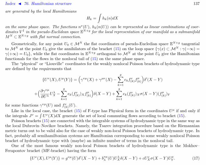
Index J 76. Hamiltonian structure 137

are generated by the local Hamiltonians

Hk =

∫hk(n)dX

on the same phase space. The functions nν(U), hk(n(U)) can be represented as linear combinations of coor-dinates V I in the pseudo-Euclidean space EN+g for the local representation of our manifold as a submanifoldMN ⊂ EN+g with flat normal connection.

Geometrically, for any point U0 ∈ MN the flat coordinates of pseudo-Eucledian space EN+g tangentialto MN at the point U0 give the annihilators of the bracket (15) on the loop space γ(x) ⊂MN : γ(−∞) =γ(+∞) = U0, while the flat coordinates in EN+g orthogonal to MN at the point U0 give the Hamiltonianfunctionals for the flows in the nonlocal tail of (15) on the same phase space.

The “physical” or “Liouville” coordinates for the weakly nonlocal Poisson brackets of hydrodynamic typeare defined by the requirements that

Uν(X), Uµ(Y ) =(γνµ(X) + γµν(X)−

g∑k=1

ekfν(k)f

µ(k)

)δ′(X − Y )

+(∂γνµ∂Uλ

UλX −g∑k=1

ek(fν(k))Xfµ(k)

)δ(X − Y ) +

g∑k=1

ek(fν(k))Xσ(X − Y )(fµ(k))Y

for some functions γνµ(U) and fν(k)(U).

Like in the local case, the bracket (15) of F-type has Physical form in the coordinates Uµ if and only ifthe integrals Jν =

∫Uν(X)dX generate the set of local commuting flows according to bracket (15).

Poisson brackets (15) are connected with the integrable systems of hydrodynamic type in the same way asthe local Dubrovin–Novikov brackets. Namely, the Tsarev integration procedure based on the Riemannianmetric turns out to be valid also for the case of weakly non-local Poisson brackets of hydrodynamic type. Infact, probably all semihamiltonian systems are Hamiltonian corresponding to some weakly nonlocal Poissonbracket of hydrodynamic type with (maybe) an infinite number of terms in the nonlocal tail.

One of the most famous weakly non-local Poisson brackets of hydrodynamic type is the Mokhov–Ferapontov bracket (MF-bracket) having the form

Uν(X), Uµ(Y ) = gνµ(U)δ′(X − Y ) + bνµλ (U)UλXδ(X − Y ) + cUνXσ(X − Y )UµY . (17)

Index J 76. Hamiltonian structure 138

For bracket (17) with non-degenerate metric tensor gνµ(U) the following statements are true.

Theorem 9 ([11]). Bracket (17) is skew-symmetric if and only if the tensor gνµ is symmetric, and theconnection

Γνµλ = −gµτ bτνλis compatible with this metric: ∇λgµν ≡ 0.

Bracket (17) satisfies the Jacobi identity if and only if its connection Γνµλ is symmetric (that is the torsiontensor vanishes) and has the constant curvature equal to c, that is

Rντµλ = c(δνµδ

τλ − δτµδνλ

).

The canonical form of MF-bracket was first pointed out by M.V. Pavlov and can be written as

nν(X), nµ(Y ) = (ενδνµ − cnνnµ) δ′(X − Y )− cnνXnµδ(X − Y ) + cnνXσ(X − Y )nµY (18)

where εν are equal to ±1, and the term ενδνµ has the same signature as metric tensor gνµ(U).The functionals

Nν =

∫nνdX

are the annihilators of the bracket (18). The functional

P =1

c

∫ 1−

√√√√∣∣∣∣1− c N∑ν=1

ενnν(X)nν(X)

∣∣∣∣ dX

is the momentum generating shifts along the coordinate X [12].Geometrically, the MF-bracket corresponds to a restriction of a DN-bracket to a (pseudo-)sphere SN ∈

EN+1 of codimension 1 in the (pseudo-)Euclidean space.The general weakly-nonlocal symplectic structures have the form

Ωij(x, y) =∑k≥0

ω(k)ij (ϕ,ϕx, . . . )δ

(k)(x− y) +

g∑s=1

esq(s)i (ϕ,ϕx, . . . )σ(x− y)q

(s)j (ϕ,ϕy, . . . ) (19)

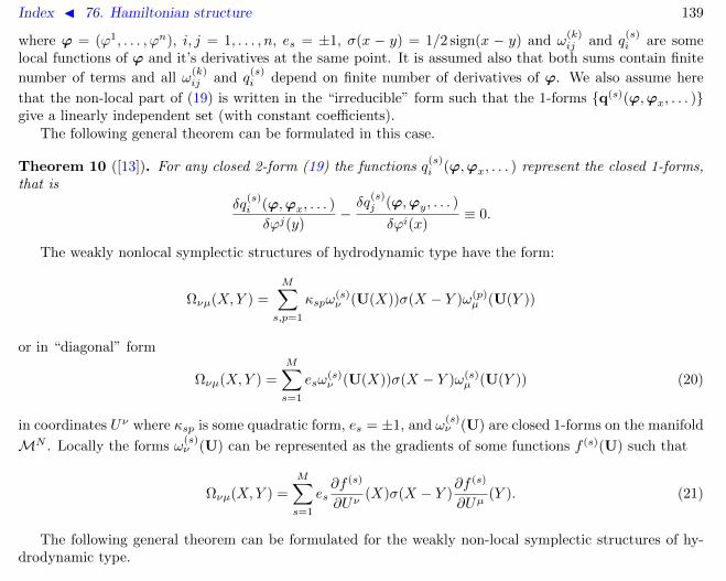
Index J 76. Hamiltonian structure 139

where ϕ = (ϕ1, . . . , ϕn), i, j = 1, . . . , n, es = ±1, σ(x − y) = 1/2 sign(x − y) and ω(k)ij and q

(s)i are some

local functions of ϕ and it’s derivatives at the same point. It is assumed also that both sums contain finite

number of terms and all ω(k)ij and q

(s)i depend on finite number of derivatives of ϕ. We also assume here

that the non-local part of (19) is written in the “irreducible” form such that the 1-forms q(s)(ϕ,ϕx, . . . )give a linearly independent set (with constant coefficients).

The following general theorem can be formulated in this case.

Theorem 10 ([13]). For any closed 2-form (19) the functions q(s)i (ϕ,ϕx, . . . ) represent the closed 1-forms,

that is

δq(s)i (ϕ,ϕx, . . . )

δϕj(y)−δq

(s)j (ϕ,ϕy, . . . )

δϕi(x)≡ 0.

The weakly nonlocal symplectic structures of hydrodynamic type have the form:

Ωνµ(X,Y ) =

M∑s,p=1

κspω(s)ν (U(X))σ(X − Y )ω(p)

µ (U(Y ))

or in “diagonal” form

Ωνµ(X,Y ) =

M∑s=1

esω(s)ν (U(X))σ(X − Y )ω(s)

µ (U(Y )) (20)

in coordinates Uν where κsp is some quadratic form, es = ±1, and ω(s)ν (U) are closed 1-forms on the manifold

MN . Locally the forms ω(s)ν (U) can be represented as the gradients of some functions f (s)(U) such that

Ωνµ(X,Y ) =

M∑s=1

es∂f (s)

∂Uν(X)σ(X − Y )

∂f (s)

∂Uµ(Y ). (21)

The following general theorem can be formulated for the weakly non-local symplectic structures of hy-drodynamic type.

Index J 76. Hamiltonian structure 140

Theorem 11 ([14, 13]). Expression (20) gives the closed 2-form on the space U(X) if and only if the

1-forms ω(s)ν (U) on MN are closed,1 that is

∂

∂Uνω(s)µ (U) =

∂

∂Uµω(s)ν (U).

The 2-form Ωνµ(X,Y ) written in form (21) can be considered as the pullback of the form

ΞIJ(X,Y ) = eIδIJσ(X − Y ), I, J = 1, . . . ,M

defined in the pseudo-Euclidean space EN with the metric GIJ = diag(e1, . . . , eM ) for the mapping α :MN → EN

(U1, . . . , UN )→ (f (1)(U), . . . , f (M)(U)).

Definition 12. We call symplectic form (20) non-degenerate if M ≥ N and

rank

ω(1)i (U). . .

ω(M)i (U)

= N.

The non-degenerate symplectic forms (20) are closely connected with the weakly nonlocal Poisson bracketsof hydrodynamic type (15). Namely, as can be shown, the symplectic form for the bracket (15) can be writtenin the form

Ωνµ(X,Y ) =

N+g∑I=1

eI∂V I

∂Uν(X)σ(X − Y )

∂V I

∂Uµ(Y )

=

N∑τ=1

eτ∂nτ

∂Uν(X)σ(X − Y )

∂nτ

∂Uµ(Y ) +

g∑k=1

ek∂hk∂Uν

(X)σ(X − Y )∂hk∂Uµ

(Y )

where V I are the coordinates in the pseudo-Euclidean space EN+g for the local representation of our manifoldas a submanifold MN ⊂ EN+g with flat normal connection [8].

1We assume that (20) is written in the “irreducible” form, i.e. the 1-forms ω(s)ν (U) are linearly independent (with constant

coefficients).

Index J 76. Hamiltonian structure 141

References

[1] V.I. Arnold. Mathematical Methods of Classical Mechanics. Springer: 1978, 1989.

[2] I.M. Gelfand, I.Ya. Dorfman. Hamiltonian operators and algebraic structures related to them. Funct. Anal.Appl. 13:4 (1979) 248–262.

[3] I.M.Gelfand, I.Ya.Dorfman. Hamiltonian operators and infinite-dimensional Lie algebras. Funct. Anal. Appl.15:3 (1981) 173–187.

[4] P.J. Olver. Applications of Lie groups to differential equations, 2nd ed., Graduate Texts in Math. 107, NewYork: Springer-Verlag, 1993.

[5] L.A. Takhtajan, L.D. Faddeev. Hamiltonian approach in the soliton theory. Moscow: Nauka, 1986.

[6] B.A. Dubrovin, S.P. Novikov. Hydrodynamics of weakly deformed soliton lattices. Differential geometry andHamiltonian theory. Russ. Math. Surveys 44:6 (1989) 35–124.

[7] B.A. Dubrovin, S.P. Novikov. Hydrodynamics of soliton lattices. Sov. Sci. Rev. C Math. Phys. 9:4 (1993) 1–136.

[8] A.Ya. Maltsev, S.P. Novikov. On the local systems Hamiltonian in the weakly nonlocal Poisson brackets. PhysicaD 156:(1–2) (2001) 53–80.

[9] A.Ya. Maltsev. The averaging of nonlocal Hamiltonian structures in Whitham’s method. Int. J. Math. Sci. 30:7(2002) 399–434.

[10] E.V. Ferapontov. Nonlocal Hamiltonian operators of hydrodynamic type: differential geometry and applications.Amer. Math. Soc. Transl. (2) 170 (1995) 33–58.

[11] O.I. Mokhov, E.V. Ferapontov. Non-local Hamiltonian operators of hydrodynamic type related to metrics ofconstant curvature. Russ. Math. Surveys 45:3 (1990) 218–219.

[12] M.V. Pavlov. Elliptic coordinates and multi-Hamiltonian structures of systems of hydrodynamic type. RussianAcad. Sci. Dokl. Math. 59:3 (1995) 374–377.

[13] A.Ya. Maltsev. Weakly-nonlocal symplectic structures, Whitham method, and weakly-nonlocal symplectic struc-tures of hydrodynamic type. J. Phys. A 38:3 (2005) 637–682.

[14] O.I. Mokhov. Symplectic and Poisson structures on loop spaces of smooth manifolds, and integrable systems.Russ. Math. Surveys 53:3 (1998) 515–622.

Index J 77. Henon–Heiles system D 142

77 Henon–Heiles system

u′′ = −au− 2duv, v′′ = −bv + cv2 − du2

ã Hamiltonian: H = 12 ((u′)2 + (v′)2 + au2 + bv2) + du2v − 1

3cv3.

ã The integrable cases: d = −c, b = a; 6d = −c; 16d = −c, b = 16a.

References

[1] J. Weiss. Backlund transformation and linearizations of the Henon–Heiles system. Phys. Lett. A 102:8 (1984)329–331.

[2] A.P. Fordy. The Henon–Heiles system revisited. Physica D 52:2–3 (1991) 204–210.

Index J 78. Hirota equation ∆∆∆ 143

78 Hirota equation

αu1u23 + βu2u13 + γu3u12 = 0, ui = Ti(u) (1)

ã The parameters may be dropped out by the scaling u(i, j, k)→ u(i, j, k) exp(λij + µik + νjk).

ã Equation (1) passes singularity confinement test [2] and possesses 4D-consistency property.

ã The auxiliary linear problems [3, 4]:

φ1 = aφ+ φ2, φ3 = bφ+ φ2 ⇒ a3 + b2 = a2 + b1, a3b = ab1.

ã Considering the equations on a, b as the conservation laws suggests the substitution

a =u12u

u1u2, b =

u23u

u2u3

which brings to (1). Conversely, eliminating a and b brings to equation

φ13 − φ12

φ1+φ12 − φ23

φ2+φ23 − φ13

φ3= 0. (2)

Equation (1) can be considered as the limiting case of Hirota–Miwa equation (80.3) while (2) correspondsto the double cross-ratio equation (80.1).

References

[1] R. Hirota. Discrete analog of a generalized Toda equation. J. Phys. Soc. Japan 50:11 (1981) 3785–3791.

[2] A. Ramani, B. Grammaticos, J. Satsuma. Integrability of multidimensional discrete systems. Phys. Lett. A169:5 (1992) 323–328.

Index J 78. Hirota equation ∆∆∆ 144

[3] O. Ragnisco, P.M. Santini, S. Chitlaru-Briggs, M.J. Ablowitz. An example of ∂-problem arising in a finitedifference context: Direct and inverse problem for the discrete analog of the equation ψxx +uψ = σψy. J. Math.Phys. 28:4 (1987) 777–780.

[4] O. Ragnisco, P.M. Santini. Recursion operator and bi-Hamiltonian structure for integrable multidimensionallattices. J. Math. Phys. 29:7 (1988) 1593–1603.

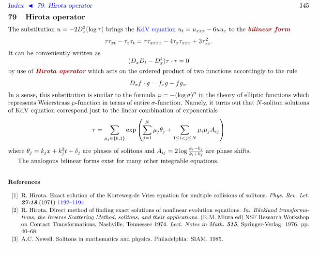
Index J 79. Hirota operator 145

79 Hirota operator

The substitution u = −2D2x(log τ) brings the KdV equation ut = uxxx − 6uux to the bilinear form

ττxt − τxτt = ττxxxx − 4τxτxxx + 3τ2xx.

It can be conveniently written as(DxDt −D4

x)τ · τ = 0

by use of Hirota operator which acts on the ordered product of two functions accordingly to the rule

Dxf · g = fxg − fgx.

In a sense, this substitution is similar to the formula ℘ = −(log σ)′′ in the theory of elliptic functions whichrepresents Weierstrass ℘-function in terms of entire σ-function. Namely, it turns out that N -soliton solutionsof KdV equation correspond just to the linear combination of exponentials

τ =∑

µj∈0,1

exp

N∑j=1

µjθj +∑

1≤i<j≤N

µiµjAij

where θj = kjx+ k3

j t+ δj are phases of solitons and Aij = 2 logki−kjki+kj

are phase shifts.

The analogous bilinear forms exist for many other integrable equations.

References

[1] R. Hirota. Exact solution of the Korteweg-de Vries equation for multiple collisions of solitons. Phys. Rev. Let.27:18 (1971) 1192–1194.

[2] R. Hirota. Direct method of finding exact solutions of nonlinear evolution equations. In: Backlund transforma-tions, the Inverse Scattering Method, solitons, and their applications. (R.M. Miura ed) NSF Research Workshopon Contact Transformations, Nashville, Tennessee 1974. Lect. Notes in Math. 515, Springer-Verlag, 1976, pp.40–68.

[3] A.C. Newell. Solitons in mathematics and physics. Philadelphia: SIAM, 1985.

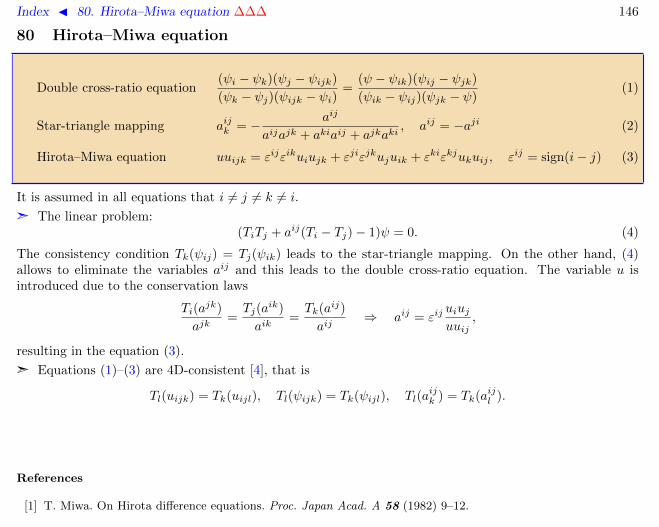
Index J 80. Hirota–Miwa equation ∆∆∆ 146

80 Hirota–Miwa equation

Double cross-ratio equation(ψi − ψk)(ψj − ψijk)

(ψk − ψj)(ψijk − ψi)=

(ψ − ψik)(ψij − ψjk)

(ψik − ψij)(ψjk − ψ)(1)

Star-triangle mapping aijk = − aij

aijajk + akiaij + ajkaki, aij = −aji (2)

Hirota–Miwa equation uuijk = εijεikuiujk + εjiεjkujuik + εkiεkjukuij , εij = sign(i− j) (3)

It is assumed in all equations that i 6= j 6= k 6= i.

ã The linear problem:(TiTj + aij(Ti − Tj)− 1)ψ = 0. (4)

The consistency condition Tk(ψij) = Tj(ψik) leads to the star-triangle mapping. On the other hand, (4)allows to eliminate the variables aij and this leads to the double cross-ratio equation. The variable u isintroduced due to the conservation laws

Ti(ajk)

ajk=Tj(a

ik)

aik=Tk(aij)

aij⇒ aij = εij

uiujuuij

,

resulting in the equation (3).

ã Equations (1)–(3) are 4D-consistent [4], that is

Tl(uijk) = Tk(uijl), Tl(ψijk) = Tk(ψijl), Tl(aijk ) = Tk(aijl ).

References

[1] T. Miwa. On Hirota difference equations. Proc. Japan Acad. A 58 (1982) 9–12.

Index J 80. Hirota–Miwa equation ∆∆∆ 147

[2] J.J.C. Nimmo, W.K. Schief. An integrable discretization of a 2+1-dimensional sine-Gordon equation. Stud. Appl.Math. 100:3 (1998) 295–309.

[3] B.G. Konopelchenko, W.K. Schief. Reciprocal figures, graphical statics and inversive geometry of the SchwarzianBKP hierarchy. Stud. Appl. Math. 109:2 (2002) 89–124.

[4] V.E. Adler, A.I. Bobenko, Yu.B. Suris. Classification of integrable equations on quad-graphs. The consistencyapproach. Commun. Math. Phys. 233 (2003) 513–543.

Index J 81. Hirota–Ohta system eDDD 148

81 Hirota–Ohta system

Authors: V.E. Adler, V.V. Postnikov, 2010.08.03

−2ut = uxxx − 3uxy + 3wux − 3qu,

−2vt = vxxx + 3vxy + 3wvx + 3qv,

4wt = wxxx − 24(uv)x + 6wwx + 3qy, qx = wy. (1)

ã Introduced by Hirota–Ohta [1], as the Pfaffianization of Kadomtsev–Petviashvili equation, see also [2].The whole hierarchy can be derived also within the general approach based on Clifford algebra representationsand the boson-fermion correspondence [3, 4].

ã Bilinear form. The change of variables

u =f

h, v =

g

h, w = 2(log h)xx, q = 2(log h)xy (2)

brings the system (1) to the form

(2Dt − 3DxDy +D3x)f · h = 0,

(2Dt + 3DxDy +D3x)g · h = 0,

(4DxDt − 3D2y −D4

x)h · h+ 24fg = 0. (3)

ã Backlund–Schlesinger transformation. System (1) admits the explicit auto-transformation

u1 = u2v +1

2(uxwx − uwy) +

w

u(uuxx − u2

x) +1

4u

(uuyy − u2

y

−2uuxxy + 2uxuxy + uuxxxx − 2uxuxxx + u2xx

),

v1 = 1/u, w1 = w + 2(log u)xx, q1 = q + 2(log u)xy. (4)

The substitutions (2) reduce the last three equations in (4) to h1 = f , g1 = h, that is the iterations of thismapping generate the sequence

. . . f = h(n1 + 1), h = h(n1), g = h(n1 − 1) . . .

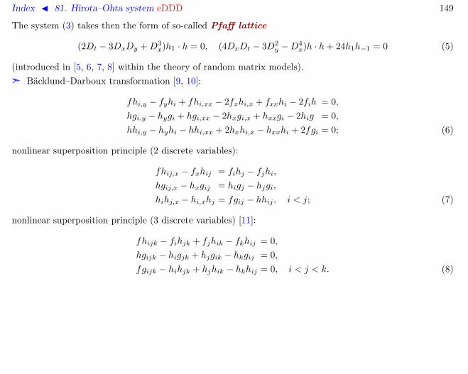
Index J 81. Hirota–Ohta system eDDD 149

The system (3) takes then the form of so-called Pfaff lattice

(2Dt − 3DxDy +D3x)h1 · h = 0, (4DxDt − 3D2

y −D4x)h · h+ 24h1h−1 = 0 (5)

(introduced in [5, 6, 7, 8] within the theory of random matrix models).

ã Backlund–Darboux transformation [9, 10]:

fhi,y − fyhi + fhi,xx − 2fxhi,x + fxxhi − 2fih = 0,

hgi,y − hygi + hgi,xx − 2hxgi,x + hxxgi − 2hig = 0,

hhi,y − hyhi − hhi,xx + 2hxhi,x − hxxhi + 2fgi = 0; (6)

nonlinear superposition principle (2 discrete variables):

fhij,x − fxhij = fihj − fjhi,hgij,x − hxgij = higj − hjgi,hihj,x − hi,xhj = fgij − hhij , i < j; (7)

nonlinear superposition principle (3 discrete variables) [11]:

fhijk − fihjk + fjhik − fkhij = 0,

hgijk − higjk + hjgik − hkgij = 0,

fgijk − hihjk + hjhik − hkhij = 0, i < j < k. (8)

Index J 81. Hirota–Ohta system eDDD 150

ã Auxiliary linear problems [12]:

ψy = ψxx + wψ + 2uφ, −φy = φxx + 2vψ + wφ;

ψt = ψxxx +3

2wψx +

3

4(wx + q)ψ + 3uxφ, φt = φxxx +

3

2wφx +

3

4(wx − q)φ+ 3vxψ;

ψ1 = ψxx −uxuψx +

(w +

uxx − uy2u

)ψ + uφ, φ1 = − 1

uψ;

ψx = ψi + w(i)ψ + uφi, −φi,x = φ+ viψ + w(i)φi;

ψj = ψi + w(ij)(ψ + uφij), φj = φi − w(ij)(vijψ + φij), i ≤ j

where

w(i) =hi,xhi− hx

h, w(ij) =

hhijhihj

.

ã Squared eigenfunctions constraint: see Kulish–Sklyanin system.

References

[1] R. Hirota, Y. Ohta. Hierarchies of coupled soliton equations. I. J. Phys. Soc. Japan 60 (1991) 798–809.

[2] J. Hietarinta. Hirota’s bilinear method and partial integrability. pp. 459–478 in: Partially integrable evolutionequations in physics (R. Conte, N. Boccara eds) NATO ASI Series C310, Kluwer, 1990.

[3] M. Jimbo, T. Miwa. Solitons and infinite dimensional Lie algebras. Publ. RIMS 19:3 (1983) 943–1001.

[4] V.G. Kac, J.W. van de Leur. The geometry of spinors and the multicomponent BKP and DKP hierarchies. In“The bispectral problem”, eds J. Harnad, A. Kasman, CRM Proc. Lecture notes 14, AMS, Providence (1998)159–202.

[5] M. Adler, E. Horozov, P. van Moerbeke. The Pfaff lattice and skew-orthogonal polynomials. Int. Math. Res.Notices 1999:11 (1999) 569–588.

Index J 81. Hirota–Ohta system eDDD 151

[6] M. Adler, P. van Moerbeke. Toda versus Pfaff lattice and related polynomials. Duke Math. J. 112:1 (2002)1–58.

[7] M. Adler, T. Shiota, P. van Moerbeke. Pfaff τ -functions. Math. Ann. 322 (2002) 423–476.

[8] S. Kakei. Orthogonal and symplectic matrix integrals and coupled KP hierarchy. J. Phys. Soc. Japan 68 (1999)2875–2877.

[9] J. van de Leur. Backlund–Darboux transformations for the coupled KP hierarchy. J. Phys. A 37 (2004) 4395–4405.

[10] X.B. Hu, J.X. Zhao. Commutativity of Pfaffianization and Backlund transformations: the KP equation. InverseProblems 21 (2005) 1461–1472.

[11] C.R. Gilson, J.J.C. Nimmo, S. Tsujimoto. Pfaffianization of the discrete KP equation. J. Phys. A 34:48 (2001)10569–10575.

[12] S. Kakei. Dressing method and the coupled KP hierarchy. Phys. Lett. A 264:6 (2000) 449–458.

Index J 82. Hirota–Satsuma equation eDD 152

82 Hirota–Satsuma equation

ut = (auxx + 3au2 − 3v2)x, vt = −vxxx − 3vxu

References

[1] R. Hirota, J. Satsuma. Soliton solutions of a coupled Korteweg-de Vries equation. Phys. Lett. A 85:8–9 (1981)407–408.

[2] J. Weiss. Backlund transformation and linearizations of the Henon–Heiles system. Phys. Lett. A 102:8 (1984)329–331.

[3] J. Weiss. Modified equations, rational solutions and the Painleve property for the Kadomtsev–Petviashvili andHirota–Satsuma equations. J. Math. Phys. 26:9 (1985) 2174–2180.

Index J 83. Hyperbolic equations with third order symmetries 153

83 Hyperbolic equations with third order symmetries

Authors: A.G. Meshkov, V.V. Sokolov, 2010.06.17

1. Introduction2. Hyperbolic equations with third order symmetries3. Discussion

Here we present a complete list of nonlinear one-field hyperbolic equations that have integrable x- andy-symmetries of third order. The list includes both sine-Gordon type equations and Liouville-type equations(linearizable by differential substitutions).

In different settings, the problem of classification of some particular types of integrable hyperbolic equa-tions had been considered in [1, 2, 3].

1. Introduction

The symmetry approach to classification of integrable PDEs (see surveys [4, 5, 6] and references there) isbased on the existence of higher infinitesimal symmetries and/or conservation laws for integrable equations.This approach is especially efficient for evolution equations with one spatial variable. In particular, allintegrable equations of the form

ut = u3 + F (u2, u1, u), ui =∂iu

∂xi(1)

were described in [7, 8]. The following list of integrable equationsList:

ut = uxxx + uux, (2)

ut = uxxx + u2ux, (3)

ut = uxxx + u2x, (4)

ut = uxxx −1

2u3x + (c1e

2u + c2e−2u)ux, (5)

Index J 83. Hyperbolic equations with third order symmetries 154

ut = uxxx −3uxu

2xx

2(u2x + 1)

+ c1(u2x + 1)3/2 + c2u

3x, (6)

ut = uxxx −3uxu

2xx

2(u2x + 1)

− 3

2℘(u)ux(u2

x + 1), (7)

ut = uxxx −3u2

xx

2ux+

3

2ux− 3

2℘(u)u3

x, (8)

ut = uxxx −3u2

xx

2ux, (9)

ut = uxxx −3u2

xx

4ux+ c1u

3/2x + c2u

2x, c1 6= 0 or c2 6= 0, (10)

ut = uxxx −3u2

xx

4ux+ cu, (11)

ut = uxxx −3

4

u2xx

ux + 1+ 3uxxu

−1(√ux + 1− ux − 1)

− 6u−2ux(ux + 1)3/2 + 3u−2ux (ux + 1)(ux + 2),

(12)

ut = uxxx −3

4

u2xx

ux + 1− 3

uxx (ux + 1) coshu

sinhu+ 3

uxx√ux + 1

sinhu

− 6ux(ux + 1)3/2 coshu

sinh2 u+ 3

ux (ux + 1)(ux + 2)

sinh2 u+ u2

x(ux + 3),

(13)

ut = uxxx + 3u2uxx + 3u4ux + 9uu2x, (14)

ut = uxxx + 3uuxx + 3u2ux + 3u2x, (15)

ut = uxxx. (16)

is equivalent to one from [7]. Here (℘′)2 = 4℘3 − g2℘− g3, and k, c, c1, c2, g2, g3 are arbitrary constants.

Index J 83. Hyperbolic equations with third order symmetries 155

Remark 1. Equations (2)–(10) are integrable by the inverse scattering transform method whereas (11)–(15)are linearizable (S and C-integrable in the terminology by F. Calogero).

Remark 2. Equation (8) is equivalent to the Krichever–Novikov equation

ut = uxxx −3

2

u2xx +Q

ux

up to a transformation of the form u→ φ(u). Equation (7) is equivalent to the Calogero–Degasperis equation

ut = uxxx −1

2Q′′ ux +

3

8

((Q− u2x)x)2

ux (Q− u2x).

Here Q = c4u4 + c3u

3 + c2u2 + c1u+ c0 is an arbitrary polynomial.

The above list is complete up to transformations of the form

u→ φ(u); t→ t, x→ x+ ct; x→ αx, t→ βt, u→ λu; u→ u+ γx+ δt. (17)

The latter transformation preserves the form (1) only for equations with ∂F∂u = 0. Moreover, the linear

equations admit the transformation:

u→ u exp(αx+ βt). (18)

Since the symmetry approach is purely algebraic, the function φ and the constants c, α, β, λ, γ and δsupposed to be complex-valued. Thus, for example, we do not distinguish between equations ut = uxxx−u3

x

and ut = uxxx + u3x.

For scalar hyperbolic equations of the form

uxy = Ψ(u, ux, uy) (19)

the symmetry approach postulates the existence of both x-symmetries

ut = A(u, ux, uxx, . . . , ), (20)

Index J 83. Hyperbolic equations with third order symmetries 156

and y-symmetriesuτ = B(u, uy, uyy, . . . , ). (21)

Two equations (19) are called equivalent if they are related by transformations of the form

x↔ y; u→ φ(u); x→ αx, y → βy, u→ λu; u→ u+ γx+ δy. (22)

Here, in general, the function φ and the constants are supposed to be complex-valued. For linear equations(19) the transformations

u→ u exp(αx+ βy); u→ u+ c x y (23)

are also allowed.For the well-known integrable sin-Gordon2 equation

uxy = c1eu + c2e

−u (24)

the simplest x and y-symmetries are given by

ut = uxxx −1

2u3x, uτ = uyyy −

1

2u3y.

These evolution equations are integrable themselves (a special case of equation (5)).The general higher symmetry classification for equations (19) turns out to be a very complicated problem,

which has not been solved so far. Some important special results have been obtained in [9, 10, 11]. In general,all three functions Ψ, A,B should be found from the compatibility conditions for equations (19), (20), and(21). However, if the functions A and B are somehow fixed, then it is not difficult to verify whether thecorresponding function Ψ exists and to find it.

To describe all integrable equations (19) of the sin-Gordon type, we assume (see the section Discussion)that symmetries (20) and (21) are integrable evolution equations of the form

ut = uxxx + F (u, ux, uxx), uτ = uyyy +G(u, uy, uyy). (25)

2We do not distinguish between sin-Gordon and sinh-Gordon equations

Index J 83. Hyperbolic equations with third order symmetries 157

We take equations from List 1 one by one as x-symmetry and find all equations (19) having this symmetry.After that in each case we find the corresponding y-symmetry or verify that it do not exist. In Section 2 wepresent all hyperbolic equations with x- and y-symmetries (25) thus obtained.

Integrable hyperbolic equations can be separated in accordance to presence or absence of x and y-integrals(see the section Discussion). Consider, for instance, the Liouville equation

uxy = eu.

It is easy to verify that the function

P = uxx −1

2u2x

does not depend on y (i.e. is a function depending on x only) for any solution u(x, y) of the Liouvilleequation. Analogously, the function

Q = uyy −1

2u2y

does not depend on x.A function w(x, y, u, uy, uyy, . . .) that does not depend on x on any solution of (19) is called x-integral.

The y-integrals are defined similarly. An equation of the form (19) is called equation of the Liouville type(or Darboux integrable equation), if the equation possesses both nontrivial x- and y-integrals. Some ofthe integrable hyperbolic equations found in Section 2 are equations of the Liouville type. The generalclassification problem for Liouville type equations was considered in [11].

In contrast to the Liouville equation, the sin-Gordon equation (24) has no x- or y-integrals for non-zerovalues of the constants ci. There are two types of such equations. Equations of the first type can be reducedto the linear Klein–Gordon equation uxy = cu by differential substitutions. If an equation with the thirdorder symmetries has no integrals and does not admit linearizing substitutions, we call it equation of sin-Gordon type. Such equations are integrable by the inverse scattering method. The following equations fromthe list of Section 2 are equations of such kind:

uxy = c1eu + c2e

−u; (26)

uxy = f(u)√u2x + 1, f ′′ = cf ; (27)

Index J 83. Hyperbolic equations with third order symmetries 158

uxy =√ux

√u2y + 1; (28)

uxy =√℘(u)− µ

√u2x + 1

√u2y + 1. (29)

Here (℘′)2 = 4℘3 − g2℘− g3, 4µ3 − g2µ− g3 = 0 and c, c1, c2, a, µ, g2, g3 are constants. Equations (27), (28),(29) are related to equation (26) via differential substitutions [11, 14, 13].

2. Hyperbolic equations with third order symmetries

Theorem 3. Suppose both x- and y-symmetry of a hyperbolic equation of the form (19) belong to the list(2)–(16) up to transformations (17), (18). Then this equation belongs to the following list:

uxy = f(u)√u2x + 1, f ′′ = cf, (30)

uxy = aeu + be−u, (31)

uxy =√ux

√u2y + 1, (32)

uxy =√u2x + 1

√u2y + 1, (33)

uxy =√℘(u)− µ

√u2x + 1

√u2y + a, (34)

uxy = 2uux, (35)

uxy = 2ux√uy, (36)

uxy = ux

√u2y + 1. (37)

uxy =√uxuy, (38)

uxy =ux(uy + a)

u, a 6= 0, (39)

uxy = (aeu + be−u)ux, (40)

uxy = uyη sinh−1 u(η eu − 1

), (41)

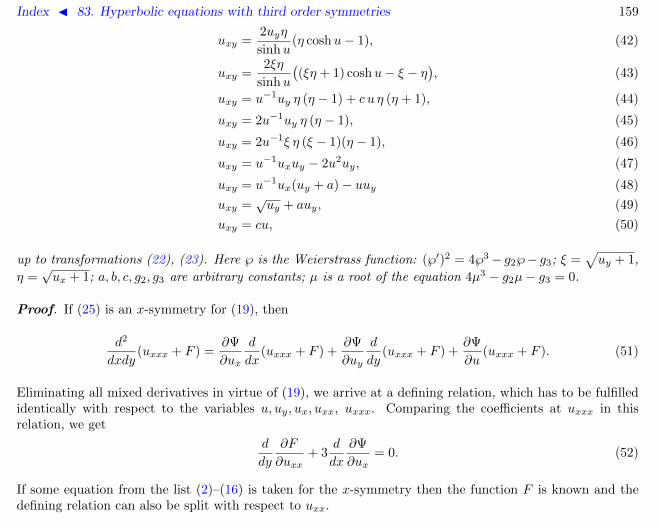
Index J 83. Hyperbolic equations with third order symmetries 159

uxy =2uyη

sinhu(η coshu− 1), (42)

uxy =2ξη

sinhu

((ξη + 1) coshu− ξ − η

), (43)

uxy = u−1uy η (η − 1) + c u η (η + 1), (44)

uxy = 2u−1uy η (η − 1), (45)

uxy = 2u−1ξ η (ξ − 1)(η − 1), (46)

uxy = u−1uxuy − 2u2uy, (47)

uxy = u−1ux(uy + a)− uuy (48)

uxy =√uy + auy, (49)

uxy = cu, (50)

up to transformations (22), (23). Here ℘ is the Weierstrass function: (℘′)2 = 4℘3− g2℘− g3; ξ =√uy + 1,

η =√ux + 1; a, b, c, g2, g3 are arbitrary constants; µ is a root of the equation 4µ3 − g2µ− g3 = 0.

Proof. If (25) is an x-symmetry for (19), then

d2

dxdy(uxxx + F ) =

∂Ψ

∂ux

d

dx(uxxx + F ) +

∂Ψ

∂uy

d

dy(uxxx + F ) +

∂Ψ

∂u(uxxx + F ). (51)

Eliminating all mixed derivatives in virtue of (19), we arrive at a defining relation, which has to be fulfilledidentically with respect to the variables u, uy, ux, uxx, uxxx. Comparing the coefficients at uxxx in thisrelation, we get

d

dy

∂F

∂uxx+ 3

d

dx

∂Ψ

∂ux= 0. (52)

If some equation from the list (2)–(16) is taken for the x-symmetry then the function F is known and thedefining relation can also be split with respect to uxx.

Index J 83. Hyperbolic equations with third order symmetries 160

For example, let equation (7) be an x-symmetry for (19). Then the uxx-splitting of (52) gives rise to:

(u2x + 1)2 ∂

2Ψ

∂u2x

− ux(u2x + 1)

∂Ψ

∂ux+ (u2

x − 1)Ψ = 0,

(u2x + 1)

(Ψ

∂2Ψ

∂ux∂uy+ ux

∂2Ψ

∂u∂ux

)− u2

x

∂Ψ

∂u− uxΨ

∂Ψ

∂uy= 0.

The general solution of this system is given by

Ψ =√u2x + 1

(g(u, uy) + C ln(ux +

√u2x + 1)

).

Substituting this expression into (51) and finding the coefficient at u3xx, we obtain C = 0 and therefore

Ψ = g(u, uy)√u2x + 1. (53)

Splitting (51) with respect to uxx and ux, we obtain that (51) is equivalent to a system consisting of (53)and equations

g∂2g

∂u∂uy− ∂g

∂u

∂g

∂uy= 0, ℘′(u)uy = 2

∂g

∂u

∂g

∂uy,

g2 ∂2g

∂u2y

+ g

(∂g

∂uy

)2

− 3g℘+∂2g

∂u2= 0,

(54)

where (℘′)2 = 4℘3 − g2℘ − g3. Since ℘′ 6= 0 we have gu 6= 0 and guy6= 0. It follows from the first two

equations (54) that g =√℘(u)− µ

√u2y + a, where µ and a are constants of integration. The third equation

is equivalent to the algebraic equation 4µ3 − g2µ− g3 = 0 for µ. Thus, we get equation (34).To prove Theorem 1 we perform similar computations for each equation from the list (2)–(15) taken

for x-symmetry. For equations (2), (4), and (8) the corresponding hyperbolic equation does not exist. Incontrast, equation (12) is an x-symmetry for several different hyperbolic equations. Indeed, in this casecalculating the coefficient at uxx in (52), we get

2(ux + 1)2 ∂2Ψ

∂u2x

− (ux + 1)∂Ψ

∂ux+ Ψ = 0,

Index J 83. Hyperbolic equations with third order symmetries 161

which implies Ψ = f1(u, uy)(ux + 1) + f2(u, uy)√ux + 1. Substituting this into (52), we obtain(

u∂f1

∂uy− 1

)(u2f1

∂f1

∂uy− 3uf1 + 2uy

)= 0,

u2

(f1∂f1

∂uy+∂f1

∂u

)− 2uf1 + 2uy = 0,

f2 = 2f1 −2

uuy − uf1

∂f1

∂uy.

If the first factor in the first equation is equal to zero, we arrive at (44). If the second factor equals zero,then we find that

f1 =2uy√auy + 1

u(1 +√auy + 1)

,

where a is a constant. The case a 6= 0 corresponds to (46), while a = 0 leads to equation (44) with c = 0.The limit a→∞ gives us equation (45).

The computations for remaining x-symmetries from the list except for the Swartz-KdV equation (9) arevery similar and we do not display them here.

Consider the Swartz-KdV equation (9). This equation is exceptional because there is a wide class ofhyperbolic equations with x-symmetry (9). We find all equations from this class that have y-symmetries.

It is easy to verify that equation

uxy = f(u, uy)ux (55)

has the following symmetry

ut = uxxx −3u2

xx

2ux+ q(u)u3

x, (56)

where (∂

∂u+ f

∂

∂uy

)2

f + 2qf + q′uy = 0. (57)

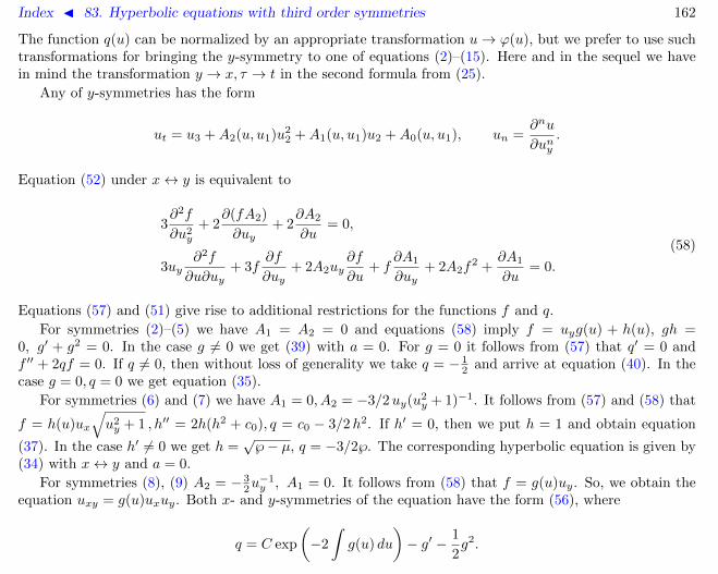
Index J 83. Hyperbolic equations with third order symmetries 162

The function q(u) can be normalized by an appropriate transformation u→ ϕ(u), but we prefer to use suchtransformations for bringing the y-symmetry to one of equations (2)–(15). Here and in the sequel we havein mind the transformation y → x, τ → t in the second formula from (25).

Any of y-symmetries has the form

ut = u3 +A2(u, u1)u22 +A1(u, u1)u2 +A0(u, u1), un =

∂nu

∂uny.

Equation (52) under x↔ y is equivalent to

3∂2f

∂u2y

+ 2∂(fA2)

∂uy+ 2

∂A2

∂u= 0,

3uy∂2f

∂u∂uy+ 3f

∂f

∂uy+ 2A2uy

∂f

∂u+ f

∂A1

∂uy+ 2A2f

2 +∂A1

∂u= 0.

(58)

Equations (57) and (51) give rise to additional restrictions for the functions f and q.

For symmetries (2)–(5) we have A1 = A2 = 0 and equations (58) imply f = uyg(u) + h(u), gh =0, g′ + g2 = 0. In the case g 6= 0 we get (39) with a = 0. For g = 0 it follows from (57) that q′ = 0 andf ′′ + 2qf = 0. If q 6= 0, then without loss of generality we take q = − 1

2 and arrive at equation (40). In thecase g = 0, q = 0 we get equation (35).

For symmetries (6) and (7) we have A1 = 0, A2 = −3/2uy(u2y + 1)−1. It follows from (57) and (58) that

f = h(u)ux√u2y + 1 , h′′ = 2h(h2 + c0), q = c0 − 3/2h2. If h′ = 0, then we put h = 1 and obtain equation

(37). In the case h′ 6= 0 we get h =√℘− µ, q = −3/2℘. The corresponding hyperbolic equation is given by

(34) with x↔ y and a = 0.

For symmetries (8), (9) A2 = − 32u−1y , A1 = 0. It follows from (58) that f = g(u)uy. So, we obtain the

equation uxy = g(u)uxuy. Both x- and y-symmetries of the equation have the form (56), where

q = C exp

(−2

∫g(u) du

)− g′ − 1

2g2.

Index J 83. Hyperbolic equations with third order symmetries 163

The equation can be reduced to the d’ Alembert equation uxy = 0 by the transformation

u =

∫du exp

(−∫g(u) du

).

For symmetries (10) and (11) A2 = − 34u−1y , A1 = 0. It follows from (58), (57) that f = g(u)uy +

C√uy, gC = 0, qC = 0, g′ + g2 = 0, q′ + 2qg = 0. If C 6= 0, then q = g = 0. Taking C = 2, we get (36). If

C = 0, then g = u−1, q = c0u−2, and we arrive at (39) with a = 0.

If the y-symmetry has the form (12), then it follows from (57), (58) that f = ku−1(uy + 1−√uy + 1),

(k − 1)(k − 2) = 0, q = 3(2− k)/(8u2). If k = 1 we get (44) up to x↔ y. The case k = 2 leads to (45).In the case of y-symmetry (13) the system of equations (57), (58) has two solutions corresponding to

equations (41), (42) with x↔ y.Symmetry (14) gives rise to equation (47) up to x↔ y.Symmetry (15) corresponds to the following equation

uxy =uxuyu+ a

− (u+ a)ux.

The shift u→ u− a brings it to a special case of equation (48).Considering the linear x-symmetry (16), we obtain equation (39) with an arbitrary parameter a, equation

(50), and

uxy = a ux + f(uy − a u), (59)

where f satisfies some nonlinear third order ODE. The requirement of existence of a y-symmetry leads to(49).

More detailed information on each equation from the list (30)–(50) can be found in Appendix 1.

3. Discussion

The hyperbolic equations of the form (19) that have both x and y-integrals were described in [11]. Inparticular, it was shown that any such equation possesses both x and y higher symmetries depending on

Index J 83. Hyperbolic equations with third order symmetries 164

arbitrary functions. Although not all of these symmetries are integrable evolution equation, there existintegrable symmetries among of them.

There are integrable equations having only y-integrals (or only x-integrals). An example of such equationis given by (34) with a = 0. Namely, the equation

uxy = ξ′(u)uy√u2x + 1, (60)

where ξ′(u) =√℘− µ, has the following first order y-integral

I = (ux +√u2x + 1 ) e−ξ

and has no x-integrals for non-degenerate Weierstrass function ℘. Notice that the same formula gives ay-integral for (60) with arbitrary function ξ.

In some sense equations (19) having integrals can be reduced to ODEs. If we are looking for equations (19)integrable by the inverse scattering transform method, we should concentrate on integrable equations (19)without integrals. There are two classes of such equations. The first one consists of the Klein–Gordon equa-tionuxy = cu, c 6= 0 and equations related to it via differential substitutions. The symmetries for such equationsare C-integrable in Calogero’s terminology.

The second class of hyperbolic integrable equations having no integrals contains equations that cannotbe reduced to a linear form by differential substitutions. This most interesting class consists of equationsadmitting only S-integrable higher symmetries. Such equations can be regarded as S-integrable hyperbolicequations.

At first glance the anzats (25) seems to be very restrictive if we want to describe all S-integrable equations(19). The first question is: why are only third order equations taken for symmetries? We can justify this inthe following way. All known S-integrable hierarchies of evolution equations (20) contain either a third orderor a fifth order equation. For polynomial hierarchies this is not an observation but a rigorous statement[12]. That is why it is enough to consider hyperbolic equations with symmetries of the third order (sin-Gordon type equations) and hyperbolic equations with fifth order symmetries (Tzitzeica type equations).The following Tzitzeica-type S-integrable equations are known up until now [11, 15]:

uxy = c1eu + c2e

−2u, (61)

Index J 83. Hyperbolic equations with third order symmetries 165

uxy = S(u)f(ux)g(uy), (62)

uxy = h(u) g(uy), h′′ = 0, (63)

where(f + 2ux)2(ux − f) = 1, (g + 2uy)2(uy − g) = 1,

(S′ − 2S2)2(S′ + S2) = c1, ω′2 = 4ω3 + c2.

We are planning to consider the Tzitzeica type equations in a separate paper.The second question is: why do we restrict ourselves by symmetries ut = uxxx + F (u, ux, uxx) instead of

general symmetries of the formut = Φ(u, ux, uxx, uxxx) ? (64)

The main reason is the following statement (see [16]). Suppose that equation (64) is a symmetry for equation(19), then

d

dy

(∂Φ(u, ux, uxx, uxxx)

∂uxxx

)= 0.

Therefore, if we assume that (19) has no nontrivial integrals, then

∂Φ(u, ux, uxx, uxxx)

∂uxxx= const.

.

Appendix 1. Symmetries, integrals and differentialsubstitutions

Here we give more information on equations from the list (30)–(50). Integrable third order symmetries,x-integrals J(u, uy, uyy, . . . ), y-integrals I(u, ux, uxx, . . . ) and, in some cases, general solutions are presented.

Equation (30). The symmetries have the following form:

ut = uxxx −c

2u3x −

3

2f2(u)ux, ut = uyyy −

3uyu2yy

2(u2y + 1)

− c

2u3y.

Index J 83. Hyperbolic equations with third order symmetries 166

The formula (30) describes two non-equaivalent sin-Gordon type equations:(30a). uxy = u

√u2x + 1 ; (30b). uxy = sinu

√u2x + 1

and two Liouville type equations:(30c). uxy =

√u2x + 1 ; the integrals are:

I =uxx√u2x + 1

, J = uyy − u;

the linearizing substitution ux = sinh(y + vx) reduces the equation to the linear one: ???. The generalsolution is given by:

u =

∫sinh(y + f(x)) dx+ g(y);

(30d). uxy = eu√u2x + 1; the integrals are:

I =uxx√u2x + 1

−√u2x + 1, J = uyy −

1

2u2y −

1

2e2u.

The general solution is given by

u(x, y) = ln

(−ϕ(x)g′(y)(

g(y) + h(x))(ϕ(x) + f(x)

(g(y) + h(x)

))) ,ϕ(x) = exp

(∫f(x)

4f ′(x)dx

), h(x) =

∫f ′(x)ϕ(x)

f2(x)dx.

Equation (31). Both x- and y-symmetries have the form (5), where c1 = c2 = 0. If ab 6= 0, then wehave the sin-Gordon equation. There is the following degeneration:

(31a). uxy = eu is the Liouville equation. Its integrable symmetries have the same form as for thesin-Gordon equation. The integrals were shown in the Introduction. The general solution

u(x, y) = log

(2f ′(x)g′(y)

(f(x) + g(y))2

)

Index J 83. Hyperbolic equations with third order symmetries 167

was found by Liouville in 1853.Equation (32). The x-symmetry has the form (10), where c1 = 0, c2 = −3/4; the y-symmetry is of the

form (6), where c1 = c2 = 0. It is an S-integrable equation.Equation (33). Both x- and y-symmetries have the form (6), where c1 = 0, c2 = −1/2. It is an

S-integrable equation.Equation (34). The x-symmetry is of the form (7), the form of the y-symmetry is analogous:

uτ = uyyy −3uyu

2yy

2(u2y + a)

− 3

2℘(u)uy(u2

y + a).

If a = 0, then this symmetry is equivalent to (9).In the general case the equation can be rewritten using the Jacobi function sn as:

uxy =1

sn(u, k)

√u2x + 1

√u2y + a. (65)

This is an S-integrable equation except for the degenerate cases considered below. Notice that the formulas√℘(u, g2, g3)− µ1 =

cn(u, k)

sn(u, k),√℘(u, g2, g3)− µ2 =

cn(u, k)

dn(u, k)

lead to another forms of equation (65). They look different but can be reduced to (65) by substitutions ofthe form (u, k)→ (λu, f(k)) (see [17], Sec. 13.22).

There are two degenerations of the Weierstrass function. In the first case when ℘(u) = u−2 we haveµ = 0 and

√℘− µ = u−1. In the second case ℘(u) = sin−2 u− 1

3 , µ = − 13 and

√℘− µ = sin−1 u.

(34a). Equation uxy = u−1√u2x + 1

√u2y + a is C-integrable, the integrals are:

I =uxx√u2x + 1

+1

u

√u2x + 1, J =

uyy√u2y + a

+1

u

√u2y + a.

The general solution is given by:

u(x, y) =√f(x) + g(y)

(−∫

dx

f ′(x)− a

∫dx

g′(y)

)1/2

.

Index J 83. Hyperbolic equations with third order symmetries 168

(34b). Equation uxy = (sinu)−1√u2x + 1

√u2y + a is C-integrable, the integrals are:

I =uxx√u2x + 1

+ cotu√u2x + 1, J =

uyy√u2y + a

+ cotu√u2y + a.

If a = 0, then the general solution is

u(x, y) = 2 arccos

(f(x) + h(x) + g(y)

2f(x)

)1/2

, h(x) =

∫ √f ′2 − f2 dx.

If a 6= 0, then the general solution is given by

u(x, y) = arccos Ψ(x, y),

Ψ(x, y) =1

2w(x)

[eg(ξ + h)2 − e−g

](2w′ + fw) + (ξ + h)eg, g = g(y),

h(y) =

∫e−g√g′2 − a dy, f ′(x) =

1

2(1 + f2)− 2

w′′

w, ξ(x) =

∫dx

w2(x).

(34c). a = 0, uxy = f(u)uy√u2x + 1. There exists the following y-integral

I = (ux +√u2x + 1) exp(−ξ(u)), ξ(u) =

∫f(u) du.

The integration with respect to y leads to the following ODE:

ux =1

2

(h(x)eξ −

(h(x)eξ

)−1).

All remaining equations are C-integrable. Some of them have two integrals and can be integrated in aclosed form. Others have no integrals and can be reduced to the linear Klein–Gordon equation.

Equation (35). The x-symmetry has the form (9) and the y-symmetry is the mKdV equation uτ =uyyy − 6u2uy. The integrals are:

I =uxxxux− 3u2

xx

2u2x

, J = uy − u2.

Index J 83. Hyperbolic equations with third order symmetries 169

The general solution is given by

u(x, y) =g′′(y)

2g′(y)− g′(y)

f(x) + g(y).

Equation (36). The x-symmetry has the form (9) and the y-symmetry is (10), where c1 = 0, c2 = −3.The integrals are:

I =uxxxux− 3u2

xx

2u2x

, J =√uy − u.

The general solution is given by

u(x, y) = − g′(y)

f(x) + g(y)+

∫(g′′)2

4g′2dy.

Equation (37). The y-symmetry has the form (6), where c1 = 0, c2 = −1/2 and the x-symmetry is

ut = uxxx −3u2

xx

2ux− 1

2u3x.

This symmetry can be reduced to (9) by u→ lnu. The integrals are:

I =uxxxux− 3u2

xx

2u2x

− 1

2u2x, J = (uy +

√u2y + 1 )e−u.

The general solution is given by

u(x, y) = ln

[1 +

g(y)

f(x) + h(y)

]+

∫g−1

√g′2 − g2 dy, h = −1

2g − 1

2

∫ √g′2 − g2 dy.

Equation (38) (the Goursat equation). Both x- and y-symmetries have the form (11) with arbitraryconstant c.

The equation is reduced to the Klein–Gordon equation vxy = 14v by any of the following two differential

substitutions:(1) ux = 4v2

x, uy = v2; (2) ux = v2, uy = 4v2y.

Index J 83. Hyperbolic equations with third order symmetries 170

Equation (39). The x-symmetry has the form (11), where c = 0 and the y-symmetry can be obtainedfrom (5) by the substitution c2 = 0, u → − lnu. Moreover, there exists the following second order y-symmetry uτ = uyy − 2u−1(u2

y + auy).The integrals and the general solution are:

I =uxxux

, J =uy + a

u; u(x, y) =

f(x)− ag(y)

g′(y).

Equation (40). The x-symmetry has the form (56), where q = − 12 and the y-symmetry is given by (5),

where c1 = − 32a

2, c2 = − 32b

2. The integrals are:

I =uxxxux− 3u2

xx

2u2x

− 1

2u2x, J = uy − aeu + be−u.

In the case a 6= 0 the general solution is given by

u(x, y) = ln g(y) + ln

[1 +

h(y)

f(x)− aϕ(y)

], lnh =

∫(ag + bg−1) dy, ϕ =

∫gh dy;

if a = 0 then

u(x, y) = lnf(x)− bg(y)

g′(y).

Equation (41). The x-symmetry has the form (13). There are the following y-symmetries:

ut = uyyy −3

2(3 + cothu)uyuyy +

1

4(3 coth2 u+ 6 cothu+ 7)u3

y,

ut = uyy −1

2(3 + cothu)u2

y.

The integrals are:

I =e−uη2 − 2η + eu

sinhu, J =

uyyuy− 1

2uy(cothu+ 3).

Index J 83. Hyperbolic equations with third order symmetries 171

The general solution is given by:

u(x, y) = −1

2ln(1 + ψ2), ψ = f(x)(g(y) + h(x)), f ′ = f − 1

4f3h′2.

Equation (42). The x-symmetry has the form (13). There are the following y-symmetries:

ut = uyyy − 6uyuyy cothu+ 2(3 coth2 u− 1)u3y, ut = uyy − 2u2

y cothu.

The integrals are:

I =η − eu

η − e−u, J =

uyyuy− 2uy cothu.

The general solution is:

u(x, y) =1

2ln

∣∣∣∣ψ + 1

ψ − 1

∣∣∣∣ , ψ = f(x)(g(y) + h(x)), h′ = −f′2 + 4f2

4f3.

Equation (43). Both x- and y-symmetries have the form (13). The equation is reduced to the Klein–Gordon equation vxy = v by the following differential substitution:

ux =(v−1vx sinhu+ coshu

)2 − 1, uy =(v−1vy sinhu+ coshu

)2 − 1.

Equation (44). There are x-symmetry of the form (12) and the following y-symmetry:

uτ = uyyy −3uyuyy

2u+

3u3y

4u2− 3c

4(2uuyy + 2u2

y − cu2uy).

The equation can be reduced to the Klein–Gordon equation vxy = cv by the following differential substitution:

u = v2/z, zx = −v2x, zy = −cv2.

If c = 0 then the Klein–Gordon equation is reduced to the d’Alembert equation and the following twointegrals appear:

I =(η − 1)2

u, J =

uyyuy− uy

2u.

Index J 83. Hyperbolic equations with third order symmetries 172

The general solution is:

u(x, y) =(f(x) + g(y))2

z(x), z(x) = −

∫f ′2(x) dx.

Notice that if c = 0 the equation admits a second order symmetry.Equation (45). There are x-symmetry of the form (12) and the following two y-symmetries:

uτ = uyyy − 6u−1uyuyy + 6u−2u3y, uτ = uyy − 2u−1u2

y.

The integrals and the general solution are given by:

I =η − 1

u, J =

uyyuy− 2

uyu

; u(x, y) =f2(x)

h(x) + g(y), h(x) = −

∫f ′2(x) dx.

Equation (46). Both x- and y-symmetries have the form (12). The integrals are of the form:

I =uxx

η(η − 1)− 2

uη(η − 1), J =

uyyξ(ξ − 1)

− 2

uξ(ξ − 1).

The general solution is given by:

u(x, y) =(f(x) + g(y))2

z(x, y), z(x, y) = −

∫f ′2(x) dx−

∫g′2(y) dy.

Equation (47). There are x-symmetry of the form (14) and the following two y-symmetries:

uτ = uyyy − 9u−1uyuyy + 12u−2u3y, uτ = uyy − 3u−1u2

y.

The integrals are of the form:

I =uxu

+ u2, J =uyyuy− 3

uyu.

The general solution is:

u(x, y) =

(f ′(x)

2(f(x) + g(y)

))1/2

.

Index J 83. Hyperbolic equations with third order symmetries 173

Equation (48). There are x-symmetry of the form (15) and the following two y-symmetries:

uτ = uyyy − 3u−1(2uy + a)uyy + 3au−2uy(3uy + a) + 6u−2u3y, uτ = uyy − 2u−1uy(uy + a).

When a = 0 the y-symmetry (9) is also admitted. The equation can be reduced to the Klein–Gordonequation vxy = −av by the following substitution:

ux =(vxv− u)

(u− λ), uy =1

λ

(uvyv

+ a)

(u− λ),

where λ is arbitrary parameter. If a = 0, then the Klein–Gordon equation is reduced to the d’Alembertequation and the following two integrals appear:

I =uxu

+ u, J =uyyuy− 2

uyu.

In this case there exists the general solution of the form u(x, y) = f ′(x)(f(x) + g(y))−1.Equation (49). The x-symmetry is ut = uxxx − 3

2 a uxx and the y-symmetry has the form (11), wherec = 0 and x is replaced by y. The integrals are of the form:

I = uxxx −3

2a uxx +

a2

2ux, J =

uyya uy +

√uy.

The general solution is given by:

u(x, y) = f(x) + eax∫ (

g(y) +1− e−ax/2

a

)dy.

The limit a→ 0 is admited here.Equation (50). There are infinitely many symmetries of the form ut = P (∂x, ∂y)u, where P is an

arbitrary polynomial with constant coefficients. In particular, there exist x- and y-symmetries of the formut = P1(∂x)u and ut = P2(∂y)u . If c 6= 0 integrals do not exist otherwise the simplest integrals are: I = ux,J = uy.

Index J 83. Hyperbolic equations with third order symmetries 174

References

[1] A.V. Zhiber, N.H. Ibragimov, A.B. Shabat. Liouville type equations. DAN SSSR 249:1 (1979) 26–29.

[2] A.V. Zhiber, A.B. Shabat. Nonlinear Klein–Gordon equations with nontrivial group. Dokl. Akad. Nauk SSSR247:5 (1979) 1103–1107.

[3] A.V. Zhiber, A.B. Shabat. The systems ux = p(u, v), vy = q(u, v) possessing symmetries. Dokl. Akad. NaukSSSR 277:1 (1984) 29–33.

[4] Sokolov V V and Shabat A B, Classification of Integrable Evolution Equations, Soviet Scientific Reviews,Section C, 4 (1984), 221–280.

[5] Mikhailov A V, Shabat A B and Yamilov R I, The symmetry approach to the classification of non-linearequations. Complete lists of integrable systems, Russian Math. Surveys, 42, 4 (1987), 1–63.

[6] Mikhailov A V, Sokolov V V and Shabat A B, The symmetry approach to classification of integrableequations, in What is Integrability? Editor: Zakharov V E, Springer series in Nonlinear Dynamics, 1991,115–184.

[7] Svinolupov S I and Sokolov V V, Evolution equations with nontrivial conservation laws, Func. analiz i pril.,16, 4 (1982), 86–87. [in Russian]

[8] Svinolupov S I and Sokolov V V, On conservation laws for equations with non-trivial Lie–Backlund algebra,in the book Integrable systems, Editor: Shabat A B, Ufa, BFAN SSSR, 1982, 53–67. [in Russian].

[9] Zhiber A V and Shabat A B, Klein–Gordon equations with a nontrivial group, Sov. Phys. Dokl., 247, 5(1979), 1103–1107.

[10] Zhiber A V and Shabat A B, Systems of equations ux = p(u, v), vy = q(u, v) possessing symmetries, Sov.Math. Dokl., 30 (1984), 23–26.

[11] Zhiber A V and Sokolov V V, Exactly integrable hyperbolic equations of Liouville type, Russian Math.Surveys, 56, 1 (2001), 63–106.

[12] Sanders J and Jing Ping Wang, On the Integrability of homogeneous scalar evolution equations, J. Differ-ential Equations, 147 (1998), 410–434.

[13] Borisov A V and Zykov S A, The dressing chain of discrete symmetries and proliferation of nonlinearequations, Theor. and Math. Phys, 115, 2 (1998), 530–541.

[14] Startsev S Ya, Laplace invariants of hyperbolic equations linearizable by a differential substitution. Theor.and Math. Phys, 120, 2 (1999), 1009–1018.

Index J 83. Hyperbolic equations with third order symmetries 175

[15] Borisov A V, Zykov S A and Pavlov M V, Tzitzeica equation and proliferation of nonlinear integrableequations, Theor. and Math. Phys, 131, 1 (2002), 550–557.

[16] Zhiber A V, Quasi-linear hyperbolic equations with infinite algebra of symmetries, Izvestiya RAN, ser. Math.,58, 4 (1994), 33–54.

[17] Bateman H and Erdelyi A, Higher transcendental functions. V. 3. New York, Toronto, London. Mc Grow-HillBook Company, Inc., 1955.

Index J 84. Integrability 176

84 Integrability

Integrable equations can be divided into linearizable ones and equations integrable by inverse scatteringtransform method (C- and S-integrable equations accordingly to Calogero). The following rigorous definitionis formulated in terms of the canonical series of the conservation laws.

Definition 1. If the canonical series for an evolutionary equation admitting the formal symmetry containsthe conservation laws of the unbounded order then the equation is called S-integrable, otherwise it is calledC-integrable.

It is important to notice that existence of an infinite sequence of conservation laws does not equivalent toS-integrability. In the example of the linear equation ut = u3 the function u2

n is the density of conservationlaw for all n = 1, 2, . . . . However, the formal symmetry for this equation is Dx and all canonical conservationlaws are trivial.

References

[1] What is Integrability? (V.E. Zakharov ed). Springer-Verlag, 1991.

[2] H. Flaschka, A.C. Newell, M. Tabor. Integrability. [1, pp. 73–114]

Index J 85. Integrable discretization 177

85 Integrable discretization

The problem of finding a discretization which preserves the integrability property is one of the central onesin the theory of integrable dynamical systems. The usual approaches to this problem based on discretizationof some intrinsic properties such as Lax pairs are very “individual” and not algorithmic. In contrast, Kahan–Hirota–Kimura unconventional discretization is a very straightforward one and can be applied to any Riccatitype system, but, generally, it does not guarantee the preserving of integrability property.

References

[1] Yu.B. Suris. The problem of integrable discretization: Hamiltonian approach. Basel: Birkhauser, 2003.

Index J 86. Integrable equations, history of 178

86 Integrable equations, history of

The excellent and detailed accounts on the history of such notions as soliton, higher symmetries, Backlundtransformation, Painleve property and so on can be found in [1, 3, 2, 4, 5].

1834 Russel’s discovery of great solitary wave of translation[6, 7]

1853 Liouville equation [8]

1855 Liouville definition of integrability [9]

1871 The papers of Boussinesq [10, 11]

1879 Bianchi–Lie–Backlund transformation [12, 13, 14, 15, 16]

1882 Darboux transformation [17]

1889 Kowalevski top [18]

1894 sine-Gordon equation [19, 20]

1895 The derivation of KdV equation [21]

1902 Works of Painleve and Gambier [22, 23]

1910 Tzitzeica equation [24]

1914? Toda lattice [25]

1940 Factorization method [26]

1955 Crum formula [27]

1955 Numerical experiments by Fermi, Pasta, Ulam and Tsingou [28]

1965 Issue of the term “soliton” [29]

Index J 86. Integrable equations, history of 179

1967 Inverse Scattering Transform Method [30]

1967 Darboux lattice [31]

References

[1] G.L. Lamb, jr. Backlund transformations at the turn of the century. In: Backlund transformations, the InverseScattering Method, solitons, and their applications. Lect. Notes in Math. 515, pp. 69–79. Springer-Verlag, 1976.

[2] R.K. Dodd, J.C. Eilbeck, J.D. Gibbon, H.C. Morris. Solitons and nonlinear wave equations. London: AcademicPress, 1982.

[3] R.K. Bullough, P.J. Caudrey (eds). Solitons. Topics in current physics 17, Springer-Verlag, 1980.

[4] M.J. Ablowitz, H. Segur. Solitons and the Inverse Scattering Transform. Philadelphia: SIAM, 1981.

[5] J.W. Miles. The Korteweg–de Vries equation, a historical essay. J. Fluid Mech. 106 (1981) 131–147.

[6] J.S. Russel. Report on waves. pp. 311–390 in Rept. 14th Meeting of the British Association for the Advancementod Science. London: J. Murray, 1844.

[7] G.S. Emmerson. John Scott Russel. A great Victorian engineer and naval architect. (John Murray: London,1977); Encyclopedia Britannica, 9th edn., p. 66.

[8] J. Liouville. Sur l’equation aux differences partielles d2 log λ/dudv ± λ/2a2 = 0. J. Math. Pures Appl. 18:1(1853) 71–72.

[9] J. Liouville. Note sur l’integration des equations de la dynamice. J. Math. Pures Appl. 20 (1855) 137–138.

[10] J. de Boussinesq. Theorie de l’intumescence liquid appelee onde solitaire ou de translation, se propagente dansun canal rectangulaire. Comptes Rendus Acad. Sci. Paris 72 (1871) 755–759.

[11] J. de Boussinesq. Theorie des ondes et de remous qui se propagent. J. Math. Pures et Appl., Ser. 2, 17 (1872)55–108.

[12] L. Bianchi. Ricerche sulle superficie a curvatura costante e sulle elicoidi. Ann. Scuola Norm. Sup. Pisa 2 (1879)285.

[13] S. Lie. Zur theorie der Flachen konstanter Krumnung. III, IV. Arch. Math. og Naturvidenskab 5:3 (1880) 282–306, 328–358.

Index J 86. Integrable equations, history of 180

[14] A.V. Backlund. Zur Theorie der partiellen Differentialgleichungen erster Ordnung. Math. Ann. 17:3 (1880)285–328.

[15] A.V. Backlund. Zur Theorie der Flachentransformationen. Math. Ann. 19:3 (1881) 387–422.

[16] A.V. Backlund. Om ytor med konstant negativ krokning. Lunds Universitets Ars-skrift 19 (1883).

[17] G. Darboux. Compt. Rend. 94 1456–1459.

[18] S.V. Kowalevski. Sur le probleme de la rotation d’un corps solide autour d’un point fixe. Acta Math. 12 (1889)177–232.

[19] G. Darboux. Lecons sur la theorie generale des surfaces. Paris: Gauthier-Villars, 1894.

[20] L. Bianchi. Lezioni di geometria differenziale. 3 ed., Pisa: Enrico Spoerri, 1923.

[21] D.J. Korteweg, G. de Vries. On the change of form of long waves advancing in a rectangular canal, and on anew type of long stationary waves. Phil. Mag. 39:241 (1895) 422–443.

[22] P. Painleve. Sur les equations differentielles du second ordre et d’ordre superieur dont l’integral general estuniform. Acta Math. 25 (1902) 1–86.

[23] B. Gambier. Acta Math. 33 (1909) 1–55.

[24] G. Tzitzeica. Sur une nouvelle classe de surfaces. C.R. Acad. Sci. Paris 150 (1910) 955–956.

[25] G. Darboux. Lecons sur la theorie generale des surfaces et les applications geometriques du calcul infinitesimal.T. I-IV. 3 ed., Paris: Gauthier-Villars, 1914-1927.

[26] E. Schrodinger. A method of determining quantum-mechanical eigenvalues and eigenfunctions. Proc. Roy. IrishAcad. A 46 (1940) 9–16.

[27] M.M. Crum. Associated Sturm–Liouville systems. Quart. J. Math. Oxford Ser. 2 6 (1955) 121–127.

[28] T. Dauxois. Fermi, Pasta, Ulam and a mysterious lady. arXiv:0801.1590v1

[29] N.J. Zabusky, M.D. Kruskal. Interaction of “solitons” in a collisionless plasma and the recurrence of initialstates. Phys. Rev. Let. 15:6 (1965) 240–243.

[30] C.S. Gardner, J.M. Greene, M.D. Kruskal, R.M. Miura. Method for solving the Korteweg-de Vries equation.Phys. Rev. Let. 19:19 (1967) 1095–1097.

[31] M. Toda. Vibration of a chain with nonlinear interaction. J. Phys. Soc. Japan 20 (1967) 431–436.

Index J 87. Integrable hierarchy 181

87 Integrable hierarchy

An equation is called integrable if it possesses an infinite-dimensional algebra of the generalized symmetries.This algebra is called the hierarchy of the equation under scrutiny.

In a wider sense, one considers as members of the hierarchy also the nonlocal generalized symmetries,the symmetries corresponding to nonisospectral deformations and the discrete symmetries generated by theBacklund transformations. This point of view, together with the use of differential/difference substitutionsallows to establish useful relations between equations belonging to different classes. All associated equationshave the conservation laws and zero curvature representations in common and this allows to apply the unifiedintegration methods to the whole hierarchy.

Example 1. Let us consider the potential KdV equation

ut3 = uxxx + 6u2x. (1)

It admits the higher symmetries

ut5 = uxxxxx + 20uxuxxx + 10u2xx + 40u3

x, . . .

generated by the recursion operator R = D2x + 8ux − 4D−1

x uxx. The commutative Lie algebra generated bythese flows is what is called the pot-KdV hierarchy.

The BT for equation (1) defines the dressing chain

un+1,x + un,x + (un+1 − un)2 + an = 0.

The problem of finding its periodic in n solutions turns out to be equivalent to construction problem offinite-gap solutions of KdV.

Further, the nonlinear superposition principle leads to the discrete KdV equation

(un,m − un+1,m+1)(un+1,m − un,m+1) = an − bm.

The change v = un+1,m − un,m, w = un,m+1 − un,m brings to Yang–Baxter map

v2 = −w +a1 − a2

w − v, w1 = −v +

a1 − a2

w − v,

Index J 87. Integrable hierarchy 182

and the restriction onto the even sublattice brings to the discrete Toda-type lattice∑n

an − an+1

un,n+1 − u= 0.

In the wide sense, all these equations can be considered as members of the equation (1) hierarchy.

Index J 88. Integrable mapping 183

88 Integrable mapping

Discrete Liouville theorem [1, 2]

References

[1] A.P. Veselov. Integrable mappings. Russ. Math. Surveys 46:5 (1991) 1–51.

[2] A.P. Veselov. What is an integrable mapping? In: What is Integrability? (V.E. Zakharov ed). Springer-Verlag,1991, pp. 251–272.

Index J 89. Ishimori equation eDDD 184

89 Ishimori equation

st = [s, syy − sxx] + gysx + gxsy, gxx + gyy = 2〈s, sy, sx〉, s ∈ R3, g ∈ R

A two-dimensional generalization of Heisenberg equation. It is gauge equivalent to Davey–Stewartson system[2].

References

[1] J. Ishimori. Multi-vortex solutions of a two-dimentional nonlinear wave equation. Progress of Theor. Phys. 72(1984) 33–37.

[2] V.D. Lipovsky, A.V. Shirokov. Funct. Anal. Appl. 23:3 (1989) 65–66.

Index J 90. Ito system eDD 185

90 Ito system

ut = uxxx + 6uux + 2vvx, vt = 2(uv)x

ã Zero curvature representation:

ψxx =(λ− u− v2

4λ

)ψ, ψt = (4λ+ 2u)ψx − uxψ.

References

[1] M. Ito. Symmetries and conservation laws of a coupled nonlinear wave equation. Phys. Lett. A 91:7 (1982)335–338.

Index J 91. Jordan algebra 186

91 Jordan algebra

Author: V.V. Sokolov, 04.07.2006

Jordan algebra is a commutative nonassociative algebra with the identities

a b = b a, (a b)a2 = a (b a2).

Any associative algebra A gives rise to the Jordan algebra A+ with respect to the product a b = ab + ba.Jordan algebra which is isomorphic to a subalgebra of some A+ is called special. There exist Jordan algebraswhich cannot be obtained in this way, these are called exceptional.

Example 1. Examples of simple Jordan algebras:1) gl+n , that is the algebra of all n × n matrices with respect to the multiplication X Y = XY + Y X

with the usual matrix multiplication in r.h.s..2) The space of n-dimensional vectors with respect to the multiplication

a b = 〈a, c〉b+ 〈b, c〉a− 〈a, b〉c

where 〈, 〉 is a nondegenerate symmetric bilinear form and c is a given constant vector.

Jordan algebras are related with some multifield KdV equations.

References

[1] P. Jordan. Uber eine Klasse nichtassoziativer hyperkomplexer Algebren. Nachr. Ges. Wiss. Gottingen (1932)569–575.

[2] N. Jacobson. Structure and representations of Jordan algebras. AMS Colloquium Publ. 39, Providence, 1968.

[3] K. Meyberg. Jordan-Tripelsysteme und die Koecher-Konstruktion von Lie-Algebren. Math. Zeitschrift B 115:1(1970) 58–78.

Index J 92. Jordan pair 187

92 Jordan pair

Author: V.V. Sokolov, 04.07.2006

Jordan pair s a direct sum V = V +⊕V − of vector spaces over a field F (if the spaces V + and V − coincidethen the term Jordan triple system is used) equipped with a trilinear operation

: V ± × V ∓ × V ± → V ±

which satisfies the identities

abc = cba, (1)

abcde − cdabe = abcde − cbade. (2)

The most important examples of Jordan pairs are:

2abc = 〈a, b〉c+ 〈c, b〉a, a, b, c ∈ FN , (3)

abc = 〈a, b〉c+ 〈c, b〉a− 〈a, c〉b, a, b, c ∈ FN , (4)

2abc = abc+ cba, a, c ∈ MatM,N (F), b ∈ MatN,M (F). (5)

The important role play the operators L(a, b) : V → V defined by formula

L(a, b)(c+ d) = abc − bad, a, c ∈ V +, b, d ∈ V −.

Relation (2) means that L(a, b) ∈ Der(V ). The differentiations of such type are called interior. Moreover,the identity (2) is equivalent to the commutation rule

[L(a, b), L(c, d)] = L(abc, d)− L(c, bad)

which implies that all interior differentiations form the Lie subalgebra Inder(V ) ⊆ Der(V ). An example ofexterior differentiation is given by the map

σ(a+ b) = a− b, a ∈ V +, b ∈ V −.

Index J 92. Jordan pair 188

The structure Lie algebra of the Jordan pair is defined as

strl(V ) = V ⊕Der(V )

with the commutator (a, c ∈ V +, b, d ∈ V −, F,G ∈ Der(V ))

[a+ b+ F, c+ d+G] = (F (c)−G(a)) + (F (d)−G(b)) + ([F,G] + L(a, d)− L(c, b)).

A number of multifield systems is related to the Jordan pairs: analogs of NLS, DNLS and modifiedVolterra lattice, mKdV, some examples with the rational r.h.s..

References

[1] O. Loos. Jordan pairs. Lecture Notes in Math. 480 (1975).

[2] E. Neher. Jordan triple systems by the grid approach. Lecture Notes in Math. 1280, 1987.

Index J 93. Kadomtsev–Petviashvili equation eDDD 189

93 Kadomtsev–Petviashvili equation

ut = uxxx − 6uux + 6σ2vyy, 2vx = u

ã This is probably the most famous 3D equation. It describes long water waves with weak nonlinearity anddispersion; also it can be used as a model for waves in ferromagnetic media or Bose–Einstein condensates.The review of many results can be found in the books [2, 3, 4].

ã Auxiliary linear problem [5, 6]:

σψy = ψxx − uψ, ψt = 4ψxxx −3

2uψx −

3

4(ux + 2σvy)ψ.

ã Backlund transformation (x, y-part) [7, 8]:

(vn + vn+1)x = (vn − vn+1)2 − σgn, gn,x = (vn − vn+1)y.

ã Higher symmetryut4 = uxxy − 4uuy − 2uxvy + wyyy, vx = u, wx = v.

ã Hirota bilinear form (u = 2(log f)xx):

(DxDt +D4x + 3σ2D2

y)f · f = 0.

ã N -soliton solution was found in [9]. The soliton solutions were studied also in the papers [10, 11] (analysisof the additional restrictions on the values of the parameters leading to the resonance interaction of solitons),[12, 13, 14, 15] and many others. The properties of the solutions depend essentially on the sign of σ2. Ifσ2 > 0 then the soliton solution is stable with respect to the 2-dimensional perturbations, while the caseσ2 < 0 is unstable.

ã The localized rational solution, or the lump

u = 2D2x log((x+ ay + (a2 − b2)t)2 + b2(y + 2at)2 + 3b−2),

was found in [16, 17]. The formula for the multi-lump solution was also derived there, which demonstratesthat the lumps interact without the phase shifts.

Index J 93. Kadomtsev–Petviashvili equation eDDD 190

References

[1] B.B. Kadomtsev, V.I. Petviashvili. On the stability of the solitary waves in the weak-dispersive media. Dokl.Akad. Nauk SSSR 192 (1970) 753–756.

[2] M.J. Ablowitz, H. Segur. Solitons and the Inverse Scattering Transform. Philadelphia: SIAM, 1981.

[3] V.I. Petviashvili, O.A. Pohotelov. Solitary waves in plasma and atmosphere. Moscow: Energoatomizdat, 1989.(in Russian)

[4] B.A. Kupershmidt. KP or mKP. Noncommutative mathematics of Lagrangian, Hamiltonian, and integrablesystems. Math. Surveys and Monographs 78, Providence, RI: AMS, 2000.

[5] V.S. Dryuma. On the analytic solution of the two-dimensional Korteweg-de Vries equation. JETP Lett. 19:12(1974) 753–755.

[6] V.E. Zakharov, A.B. Shabat. The scheme of integration of nonlinear equations of mathematical physics byinverse scattering method. I. Funct. Anal. Appl. 8:3 (1974) 226–235; II. 13:3 (1979) 13–22.

[7] H.H. Chen. A Backlund transformation in two dimensions. J. Math. Phys. 16:12 (1975) 2382–2384.

[8] J. Weiss. Modified equations, rational solutions and the Painleve property for the Kadomtsev–Petviashvili andHirota–Satsuma equations. J. Math. Phys. 26:9 (1985) 2174–2180.

[9] J. Satsuma. N -soliton solution of the two-dimensional Korteweg-de Vries equation. J. Phys. Soc. Japan 40(1976) 286–290.

[10] J.W. Miles. Obliquely interacting solitary waves. J. Fluid Mech. 79 (1977) 157–169.

[11] J.W. Miles. Resonantly interacting solitary waves. J. Fluid Mech. 79 (1977) 171–179.

[12] N.C. Freeman. A two dimensional distributed soliton solution of the KdV equation. Proc. Roy. Soc. Lond. A366 (1979) 185–204.

[13] N.C. Freeman. Soliton interactions in two dimensions. Adv. Appl. Mech. 20 (1980) 1–37.

[14] S.V. Manakov, P.M. Santini, L.A. Takhtajan. Asymptotic behavior of the solutions of the Kadomtsev–Petviashvili equation. Phys. Lett. A 75 (1980) 451–454.

[15] A.A. Zaitsev. On the formation of stationary nonlinear waves by superposition of solitons. Dokl. Akad. NaukSSSR 272:3 (1983) 583–587.

[16] S.V. Manakov, V.E. Zakharov, L.A. Bordag, V.B. Matveev. Two-dimensional solitons of the KP equation andtheir interaction. Phys. Lett. A 63:3 (1977) 205–206.

[17] J. Satsuma, M.J. Ablowitz. Two-dimensional lumps in nonlinear dispersive systems. J. Math. Phys. 20 (1979)1496.

Index J 94. Kadomtsev–Petviashvili equation cylindrical eDDD 191

94 Kadomtsev–Petviashvili equation cylindrical

uxt = (uxx + 3u2)xx −ux2t

+ 3σ2uyyt2

(1)

Alias: Johnson equation [3].

ã The point equivalence to KP equation [4]:

u(x, y, t) = U(x+

y2t

12σ2, yt, t

), UXT = (UXX + 3U2)XX + 3σ2UY Y .

References

[1] E. Infeld, G. Rowlands. Nonlinear waves, solitons, and chaos, 2nd ed. Cambridge Univ. Press, 1990.

[2] V. Matveev, M. Salle. Darboux transformations and solitons. Springer-Verlag, 1991.

[3] R.S. Johnson. J. Fluid Mech. 97:4 (1980) 701–719.

[4] V.D. Lipovsky, V.B. Matveev, A.O. Smirnov. Zap. Semin. LOMI 150 (1986) 70–75.

Index J 95. Kadomtsev–Petviashvili equation modified eDDD 192

95 Kadomtsev–Petviashvili equation modified

ut = uxxx − 6u2ux + 6uxvy + 3vyy, vx = u

Index J 96. Kadomtsev–Petviashvili equation matrix eDDD 193

96 Kadomtsev–Petviashvili equation matrix

ut = uxxx − 3(uux + uxu− vyy + vyu− uvy), vx = u, u ∈ Matn(R)

Index J 97. Kahan–Hirota–Kimura discretization 194

97 Kahan–Hirota–Kimura discretization

Let an ODE system with quadratic r.h.s. be given

x′ = Q(x, x) +Ax+ b, x ∈ Rn,

where Q(x, y) = Q(y, x) is a rank 3 tensor, A is a matrix and b is a vector. The discretization proposed inthe works [1, 2, 3] is given by the formula

xn+1 − xnε

= Q(xn+1, xn)−Q(xn+1, xn+1)−Q(xn, xn) +A(xn+1 + xn) + 2b,

which defines a birational mapping xn+1 = fε(xn) with the property xn = f−ε(xn+1). In general, this trickdoes not guarantee the preserving of the Liouville integrability. However, the conjecture exists that if theoriginal ODE system is algebraically completely integrable then this is true for the corresponding discreteversion as well.

Examples: Lotka–Volterra system, Euler top

References

[1] W. Kahan. Unconventional numerical methods for trajectory calculations. Unpublished lecture notes (1993).

[2] W. Kahan, R.-C. Li. Unconventional schemes for a class of ordinary differential equations — with applicationsto the Korteweg-de Vries equation. Jour. Comp. Phys. 134 (1997) 316–331.

[3] K. Kimura, R. Hirota. Discretization of the Lagrange top. J. Phys. Soc. Japan 69 (2000) 3193–3199.

Index J 98. Kaup system eDD 195

98 Kaup system

ut = uxx + 2(u+ v)ux, vt = −vxx + 2(u+ v)vx

ã Backlund transformation:

un,x = (un + vn+1)(un+1 − un + βn), vn,x = (un−1 + vn)(vn − vn−1 − βn−1)

ã Nonlinear superposition principle

un = un − (βn+1 − βn)un + vn+1

un−1 + vn+1 − βn−1, vn = vn + (βn+1 − βn)

vn + un−1

un−1 + vn+1 − βn

ã Zero curvature representation

U =

(12 (u− v) (u+ λ)(v + λ)

1 12 (v − u)

), V = (u+ v − 2λ)U +

(12 (ux + vx) λ(ux − vx) + uxv − uvx

0 − 12 (ux + vx)

),

Wn = (un + vn+1)−1/2

(un − λ unvn+1 + (λ− βn)(un + vn+1) + λ2

1 vn+1 − λ

)

References

[1] D.J. Kaup. Finding eigenvalue problems for solving nonlinear evolution equations. Progr. Theor. Phys. 54:1(1975) 72–78.

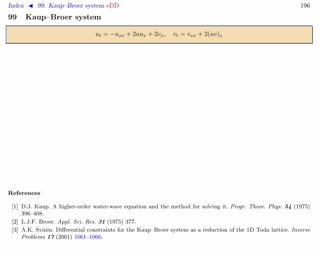
Index J 99. Kaup–Broer system eDD 196

99 Kaup–Broer system

ut = −uxx + 2uux + 2vx, vt = vxx + 2(uv)x

References

[1] D.J. Kaup. A higher-order water-wave equation and the method for solving it. Progr. Theor. Phys. 54 (1975)396–408.

[2] L.J.F. Broer. Appl. Sci. Res. 31 (1975) 377.

[3] A.K. Svinin. Differential constraints for the Kaup–Broer system as a reduction of the 1D Toda lattice. InverseProblems 17 (2001) 1061–1066.

Index J 100. Kaup–Kupershmidt equation eDD 197

100 Kaup–Kupershmidt equation

ut = u5 + 5uu3 +25

2u1u2 + 5u2u1

ã Lax pair:

L = D3x + uDx +

1

2u1, −A = 9D5

x + 15uD3x +

45

2u1D

2x +

5

2(7u2 + 2u2)Dx + 5(u3 + uu1).

ã See also: Sawada–Kotera equation

References

[1] D.J. Kaup. On the inverse scattering problem for cubic eigenvalue problems of the class ψxxx+6Qψx+6Rψ = λψ.Stud. Appl. Math. 62 (1980) 189–216.

[2] A.P. Fordy, J.D. Gibbons. Some remarkable nonlinear transformations. Phys. Lett. A 75:5 (1980) 325.

[3] V.G. Drinfeld, V.V. Sokolov. Lie algebras and equations of Korteweg-de Vries type. J. Soviet Math. 30 (1985)1975–2036.

Index J 101. Kaup–Kupershmidt equation, twodimensional eDD 198

101 Kaup–Kupershmidt equation, twodimensional

ut = u5 + 5uu3 +25

2u1u2 + 5u2u1 − 5u2,y − 5uuy − 5wu1 − 5wy, uy = wx

ã Introduced in [1].

ã Auxiliary linear problems ψy = Lψ, ψt = Aψ,

L = D3x + uDx +

1

2u1, −A = 9D5

x + 15uD3x +

45

2u1D

2x +

5

2(7u2 + 2u2 + 2w)Dx + 5(u3 + 2uu1 +

1

2uy).

ã See also: 2D Sawada–Kotera equation

References

[1] B.G. Konopelchenko, V.G. Dubrovsky. Some new integrable nonlinear evolution equations in 2 + 1 dimensions.Phys. Lett. A 102:1–2 (1984) 15–17.

Index J 102. Khokhlov–Zabolotskaya equation dDDD 199

102 Khokhlov–Zabolotskaya equation

uxt = uxuxx + uyy + uzz

Reduction uz = 0 corresponds to the dispersionless limit of KP equation.The Lagrangian: L = −uxut + 1

3u3x + u2

y + u2z.

References

[1] E.A. Zabolotskaya, R.V. Khokhlov. Quasi-plane waves in the nonlinear acoustics of confined beams. Sov. Phys.Acoust. 15 (1969) 35–40.

Index J 103. Kirchhoff system D 200

103 Kirchhoff system

u′ = [u,Hu] + [v,Hv], v′ = [v,Hu], H = 〈u,Au〉+ 〈v,Bv〉+ 〈u,Cv〉u, v ∈ R3, A,B,C ∈ Mat3(R), A = diag(a1, a2, a3), B = Bᵀ

Index J 104. Kolmogorov–Petrovsky–Piskunov equation eDD 201

104 Kolmogorov–Petrovsky–Piskunov equation

ut = uxx + δ(u− α)(u− β)(u− γ)

Alias: FitzHugh–Nagumo equation

ã Not integrable. The change x→ ax, t→ a2t, u→ bu+ c allows to bring the equation to the form

ut = uxx − u(u− 1)(u− α).

The rich families of exact solutions were found in [4, 5, 6].

See also: Burgers–Huxley, Fischer equations.

References

[1] A.N. Kolmogorov, I.G. Petrovsky, N.S. Piskunov. The study of a diffusion equation related to the increase ofthe quantity of matter, and its application to one biological problem. Bull. Univ. Moscow, Ser. Internat. Sect.A Math. mech. 1 (1937) 1–26.

[2] R. Fitzhugh. Impulses and physiological states in theoretical models of nerve membrane. Biophys. J. 1 (1961)445–466.

[3] J.S. Nagumo, S. Arimoto, S. Yoshizawa. An active pulse transmission line simulating nerve axon. Proc. IRE 50(1962) 2061–2070.

[4] R.M. Miura. Accurate computation of the stable solitary wave for the FitzHugh–Nagumo equations. J. Math.Biol. 13 (1982) 247–269.

[5] M.C. Nucci, P.A. Clarkson. The nonclassical method is more general than the direct method for symmetryreductions. An example of the Fitzhugh–Nagumo equation. Phys. Lett. A 164:1 (1992) 49–56.

[6] P.A. Clarkson, E.L. Mansfield. Symmetry reductions and exact solutions of a class of nonlinear heat equations.Physica D 70:3 (1994) 250–288.

Index J 105. Korteweg–de Vries equation eDD 202

105 Korteweg–de Vries equation

ut = uxxx + 6uux

ã This fundamental equation describes the weakly nonlinear waves in the one dimensional media withweak dispersion. Introduced in [1], it was the first nonlinear equation integrated by use of Inverse ScatteringMethod [2].

ã Higher symmetries are defined by the formula ut2n+1= Rn(ux) = u2n+1+. . . where R = D2

x+4u+2uxD−1x

is the recursion operator. For example, next two symmetries are:

ut5 = u5 − 10uu3 − 20u1u2 + 30u2u1,

ut7 = u7 − 14uu5 − 42u1u4 − 70u2u3 + 70u2u3 + 280uu1u2 + 70u31 − 140u3u1.

All higher symmetries are local and can be chosen homogeneous with respect to the weight w(un) = 2 + n.Alternatively, higher symmetries ut2n+1

= constDx(gn) can be computed by use of the generating functiong = 1 + g1/λ+ g2/λ

2 + . . . accordingly to explicit recurrent relations

gxxx + 4(λ+ u)gx + 2uxg = 0 ⇒ 2ggxx − g2x + 4(λ+ u)g2 = 4λ ⇒

8gn+1 =

n−1∑j=1

gj,xgn−j,x − 2

n−1∑j=0

gjgn−j,xx − 4

n∑j=1

gjgn+1−j − 4u

n∑j=0

gjgn−j .

ã Zero curvature representation

U =

(0 1

−u− λ 0

), Vn = (−4)n

(− 1

2Gn,x Gn− 1

2Gn,xx − (u+ λ)Gn12Gn,x

), Gn = λn + λn−1g1 + · · ·+ gn

ã Soliton solutions. A wide class of solutions is given by the formula u = 2(K(x, x, t))x where K(x, y, t) isa solution of Gelfand–Levitan–Marchenko equation

F (x+ y, t) +K(x, y, t) +

∫ ∞x

F (ξ + y, t)K(x, ξ, t)dξ = 0, x ≤ y <∞

Index J 105. Korteweg–de Vries equation eDD 203

with a kernel F (x, t) rapidly decreasing at x→ −∞ and such that Ft = −8Fxxx. In particular, the n-solitonsolutions corresponds to the degenerate kernel F (x, t) =

∑nj=1 exp(kjx+ 8k3

j t+ δj).The 1-soliton solution is given by the formula

u =2k2

cosh2(kx+ 4k3t+ δ).

The formula for the N -soliton solution [3] reads

u = 2D2x logW [ey1 + e−y1 , . . . , eyn − (−1)ne−yn ], yj = kjx+ 4k3

j t+ δj , 0 < k1 < · · · < kn

where W denotes the Wronskian W [f1, . . . , fn] = det(Di−1x (fj))

nj,i=1.

-10

0

10x-5

0

5

t

0

0.5

1

1.5

u

-10

0

10x

-40-20

0

20x -20

0

20

40

60

t

0

1

2

3

u

-40-20

0

20x

References

[1] D.J. Korteweg, G. de Vries. On the change of form of long waves advancing in a rectangular canal, and on anew type of long stationary waves. Phil. Mag. 39:241 (1895) 422–443.

Index J 105. Korteweg–de Vries equation eDD 204

[2] C.S. Gardner, J.M. Greene, M.D. Kruskal, R.M. Miura. Method for solving the Korteweg-de Vries equation.Phys. Rev. Let. 19:19 (1967) 1095–1097.

[3] H.D. Wahlquist. Backlund transformations of potentials of the Korteweg-de Vries equation and the interactionof solitons with cnoidal waves. In: Backlund transformations, the Inverse Scattering Method, solitons, and theirapplications. (R.M. Miura ed) NSF Research Workshop on Contact Transformations, Nashville, Tennessee 1974.Lect. Notes in Math. 515, Springer-Verlag, 1976, pp. 162–183.

Index J 106. Korteweg–de Vries equation cylindrical eDD 205

106 Korteweg–de Vries equation cylindrical

ut = uxxx + 6uux −u

2t(1)

ã The Lax pair [1]:

−tψxx =( x

12+ tu+ λ

)ψ, ψt = 4ψxxx + 6uψx + 3uxψ.

ã The point transformation to KdV equation [2]:

u(x, t) =1

tU(xt−1/2,−2t−1/2)− x

12t, UT = UXXX + 6UUX .

See also [4, 5]. Another equivalent form is [3]

ut = uxxx + 6t−1/2uux.

ã Recursion operator for the latter form is [6]

L = tD2x + 4t1/2u+

1

3x+ (2t1/2ux +

1

6)D−1

x .

ã Multifield generalizations were studied in [7].

References

[1] V.S. Dryuma. Izvestiya AN MSSR 1976:3 (1976) 89.

[2] A. Lugovtsov, B. Lugovtsov. Dynamika sploshnoi sredy 1 (1969) 195–200. (in Russian)

[3] F. Calogero, A. Degasperis. Lett. Nuovo Cim. 23 (1978) 150.

[4] R.S. Johnson. On the inverse scattering transform, the cylindrical Korteweg-de Vries equation and similaritysolutions. Phys. Lett. A 72:3 (1979) 197–199.

[5] V. Matveev, M. Salle. Darboux transformations and solitons. Springer-Verlag, 1991.

[6] W. Oevel, A.S. Fokas. J. Math. Phys. 25 (1984) 918.

[7] M. Gurses, A. Karasu, R. Turhan. Non-autonomous Svinolupov Jordan KdV Systems. SI/0101031 (2001).

Index J 107. Korteweg–de Vries equation Jordan eDD 206

107 Korteweg–de Vries equation Jordan

ut = uxxx + u ux, u ∈ J

where J is a Jordan algebra. The particular cases are vector and matrix KdV equations.

References

[1] S.I. Svinolupov. Jordan algebras and generalized KdV equations. Theor. Math. Phys. 87:3 (1991) 611–620.

Index J 108. Korteweg–de Vries equation matrix eDD 207

108 Korteweg–de Vries equation matrix

ut = uxxx + 3uux + 3uxu, u ∈Matn

Index J 109. Korteweg–de Vries equation modified eDD 208

109 Korteweg–de Vries equation modified

ut = uxxx ± 6u2ux

Index J 110. Korteweg–de Vries equation modified Jordan eDD 209

110 Korteweg–de Vries equation modified Jordan

ut = uxxx + u, u, ux, u ∈ J

where J Jordan triple systems.The particular cases are the following vector and matrix analogs of mKdV equation:

ut = uxxx + 〈u, u〉ux, u ∈ RN ,ut = uxxx + 〈u, u〉ux + 〈u, ux〉u, u ∈ RN ,ut = uxxx + u2ux + uxu

2, u ∈ MatN .

Index J 111. Korteweg–de Vries equation modified matrix–1 eDD 210

111 Korteweg–de Vries equation modified matrix–1

ut = uxxx + 3u2ux + 3uxu2, u ∈Matn (1)

Index J 112. Korteweg–de Vries equation modified matrix–2 eDD 211

112 Korteweg–de Vries equation modified matrix–2

ut = uxxx + 3[u, uxx] + 6uuxu, u ∈Matn (1)

References

[1] F.A. Khalilov, E.Ya. Khruslov. Matrix generalization of the modified Korteweg-de Vries equation. Inverse Prob-lems 6:2 (1990) 193–204.

[2] Q.P. Liu, C. Athorne. Comment on ‘Matrix generalization of the modified Korteweg-de Vries equation’. InverseProblems 7:5 (1991) 783–785.

Index J 113. Korteweg–de Vries equation potential eDD 212

113 Korteweg–de Vries equation potential

ut = uxxx + 6u2x

ã Substitution v = 2ux brings to KdV equation vt = vxxx + 6vvx.

ã Recursion operator: R = D2x + 8ux − 4D−1

x uxx.

ã Higher symmetry:ut = uxxxxx + 20uxuxxx + 10u2

xx + 40u3x

Index J 114. Korteweg–de Vries equation with Schwarzian eDD 213

114 Korteweg–de Vries equation with Schwarzian

ut = uxxx −3u2

xx

2ux+ aux

Most degenerate case of Krichever–Novikov equation.

Index J 115. Korteweg–de Vries equation spherical eDD 214

115 Korteweg–de Vries equation spherical

ut = uxxx + 6uux +u

t

Not integrable, in contrast to the cylindrical KdV equation.

Index J 116. Korteweg–de Vries equation, super- eDD 215

116 Korteweg–de Vries equation, super-

ut =1

4uxxx +

3

2uux + 3vvx, vt = vxxx +

3

2uvx +

3

4uxv

References

[1] B.A. Kupershmidt. A super KdV equation: an integrable system. Phys. Lett. A 102:5–6 (1984) 213–215.

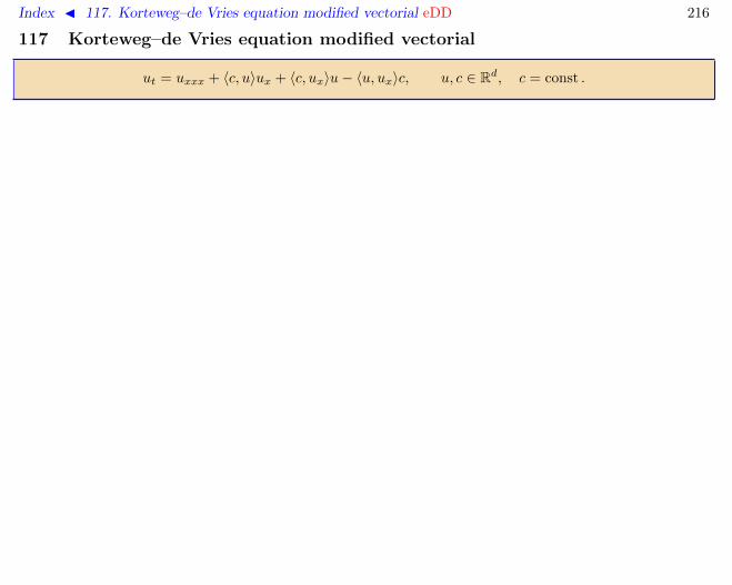
Index J 117. Korteweg–de Vries equation modified vectorial eDD 216

117 Korteweg–de Vries equation modified vectorial

ut = uxxx + 〈c, u〉ux + 〈c, ux〉u− 〈u, ux〉c, u, c ∈ Rd, c = const .

Index J 118. Korteweg–de Vries-type equations, classification eDD 217

118 Korteweg–de Vries-type equations, classification

Authors: A.G. Meshkov, V.V. Sokolov, 2009

1. The list of integrable equations2. Integrability conditions3. The classification scheme

1. The list of integrable equations

KdV-type equations are integrable third order evolutionary equations with constant separant:

ut = u3 + F (u, u1, u2), (1)

Their exhaustive classification was obtained by Svinolupov and Sokolov [1, 2] (more precisely, a bit moregeneral problem with F explicitly depending on x was solved in these papers, however, it turned out thatit did not lead to essentially new answers). The proof of the following theorem can be transformed to anintegrability test which can be applied to a given equation of the form (1). Moreover, if equation happens tobe integrable then the change of variables relating it to one of the equation in the list is found constructively.

Theorem 1. Any nonlinear integrable equation (1) is point equivalent to an equation from the following list:

ut = u3 + uu1, (K1)

ut = u3 + u2u1, (K2)

ut = u3 + u21, (K3)

ut = u3 −1

2u3

1 + (c1e2u + c2e

−2u)u1, (K4)

ut = u3 −3u1u

22

2(u21 + 1)

+ c1(u21 + 1)3/2 + c2u

31, (K5)

ut = u3 −3u1u

22

2(u21 + 1)

− 3

2P (u)u1(u2

1 + 1), (K6)

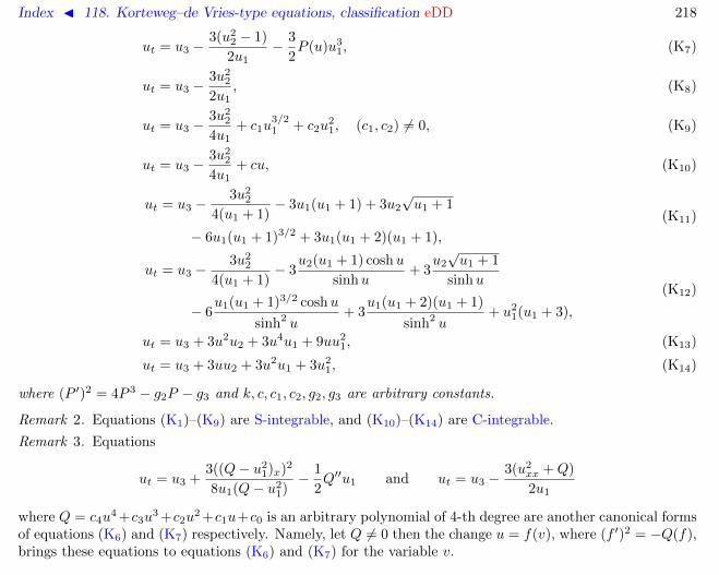
Index J 118. Korteweg–de Vries-type equations, classification eDD 218

ut = u3 −3(u2

2 − 1)

2u1− 3

2P (u)u3

1, (K7)

ut = u3 −3u2

2

2u1, (K8)

ut = u3 −3u2

2

4u1+ c1u

3/21 + c2u

21, (c1, c2) 6= 0, (K9)

ut = u3 −3u2

2

4u1+ cu, (K10)

ut = u3 −3u2

2

4(u1 + 1)− 3u1(u1 + 1) + 3u2

√u1 + 1

− 6u1(u1 + 1)3/2 + 3u1(u1 + 2)(u1 + 1),

(K11)

ut = u3 −3u2

2

4(u1 + 1)− 3

u2(u1 + 1) coshu

sinhu+ 3

u2

√u1 + 1

sinhu

− 6u1(u1 + 1)3/2 coshu

sinh2 u+ 3

u1(u1 + 2)(u1 + 1)

sinh2 u+ u2

1(u1 + 3),

(K12)

ut = u3 + 3u2u2 + 3u4u1 + 9uu21, (K13)

ut = u3 + 3uu2 + 3u2u1 + 3u21, (K14)

where (P ′)2 = 4P 3 − g2P − g3 and k, c, c1, c2, g2, g3 are arbitrary constants.

Remark 2. Equations (K1)–(K9) are S-integrable, and (K10)–(K14) are C-integrable.

Remark 3. Equations

ut = u3 +3((Q− u2

1)x)2

8u1(Q− u21)− 1

2Q′′u1 and ut = u3 −

3(u2xx +Q)

2u1

where Q = c4u4 +c3u

3 +c2u2 +c1u+c0 is an arbitrary polynomial of 4-th degree are another canonical forms

of equations (K6) and (K7) respectively. Namely, let Q 6= 0 then the change u = f(v), where (f ′)2 = −Q(f),brings these equations to equations (K6) and (K7) for the variable v.

Index J 118. Korteweg–de Vries-type equations, classification eDD 219

Remark 4. The point transformations used for bringing KdV-type equations to one of the listed above arerather simple. The whole class of equations (1) admits the following point transformations:

(conformal changes) u = φ(u), (2)

(Galilean boost) x = x+ ct, F → F − cu1, (3)

(scaling) x = ax, t = a3t, F (u, u1, u2)→ a−3F (u, au1, a2u2). (4)

Moreover, some special subclasses of equations admits additional point transforms. If function F does notdepend on u then the transformation

u = u+ c1x+ c2t, F (u1, u2)→ F (u1 − c1, u2) + c2 (5)

as admissible, and if the function F is homogeneous of the weight 1: F (λu, λu1, λu2) = λF (u, u1, u2), thenan admissible transformation is

u = u exp(at+ bx), F → F + au, un → (∂x − b)nu. (6)

The scheme of the proof presented below gives simultaneously an algorithm of reducing an integrable equationto one of the standard forms (K1)–(K14).

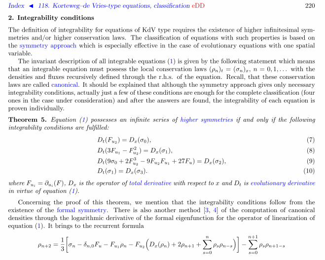
Index J 118. Korteweg–de Vries-type equations, classification eDD 220

2. Integrability conditions

The definition of integrability for equations of KdV type requires the existence of higher infinitesimal sym-metries and/or higher conservation laws. The classification of equations with such properties is based onthe symmetry approach which is especially effective in the case of evolutionary equations with one spatialvariable.

The invariant description of all integrable equations (1) is given by the following statement which meansthat an integrable equation must possess the local conservation laws (ρn)t = (σn)x, n = 0, 1, . . . with thedensities and fluxes recursively defined through the r.h.s. of the equation. Recall, that these conservationlaws are called canonical. It should be explained that although the symmetry approach gives only necessaryintegrability conditions, actually just a few of these conditions are enough for the complete classification (fourones in the case under consideration) and after the answers are found, the integrability of each equation isproven individually.

Theorem 5. Equation (1) possesses an infinite series of higher symmetries if and only if the followingintegrability conditions are fulfilled:

Dt(Fu2) = Dx(σ0), (7)

Dt(3Fu1 − F 2u2

) = Dx(σ1), (8)

Dt(9σ0 + 2F 3u2− 9Fu2

Fu1+ 27Fu) = Dx(σ2), (9)

Dt(σ1) = Dx(σ3). (10)

where Fui= ∂ui

(F ), Dx is the operator of total derivative with respect to x and Dt is evolutionary derivativein virtue of equation (1).

Concerning the proof of this theorem, we mention that the integrability conditions follow from theexistence of the formal symmetry. There is also another method [3, 4] of the computation of canonicaldensities through the logarithmic derivative of the formal eigenfunction for the operator of linearization ofequation (1). It brings to the recurrent formula

ρn+2 =1

3

[σn − δn,0Fu − Fu1

ρn − Fu2

(Dx(ρn) + 2ρn+1 +

n∑s=0

ρsρn−s

)]−n+1∑s=0

ρsρn+1−s

Index J 118. Korteweg–de Vries-type equations, classification eDD 221

− 1

3

∑0≤s+k≤n

ρsρkρn−s−k −Dx

[ρn+1 +

1

2

n∑s=0

ρsρn−s +1

3Dx(ρn)

], n ≥ 0

where δi,j is Kronecker delta and the initial data are

ρ0 = −1

3Fu2 , ρ1 =

1

9F 2u2− 1

3Fu1 +

1

3Dx(Fu2).

It is easy to check that the first four conditions from this sequence are equivalent to the conditions (7)–(10).The effective use of the canonical conservation laws for the classification is based on the preliminary

study of the possible structure of the densities of the local conservation laws for equations of the form (1).

Lemma 6. let ρ(u, u1, u2) be a conserved density for equation (1). Then

ρu2u2u2= 0, ρu2u2u1

+ ρu∗u∗u∗ =2

3Fu2

ρu2u2. (11)

The following algorithm is used in the proof in order to check, if the given function S(u, u1, . . . , un) is thetotal derivative in x (that is, belongs to ImDx) or not. First, S have to be linear in the leading derivativeun. If this is true then, as one can easily see, a total derivative can be subtracted from S in such a waythat the order of the result will be less than n. Repeating of this procedure we come either to an expressionwhich is not linear in the leading derivative or to zero.

An alternative method is based on the well-known property

S ∈ R⊕ ImDx ⇔ δS

δu= 0,

δ

δu:=

∞∑k=0

(−Dx)k∂uk

of variational derivative. Although it is more transparent theoretically, the previous method is much moreeffective for computation.

Let us show, how the formulae (11) are used in the classification of equations (1).

Lemma 7. Let equation (1) satisfies the first integrability condition (7). Then function F is quadratic inu2.

Index J 118. Korteweg–de Vries-type equations, classification eDD 222

Proof. Accordingly to the first equation (11),

Fu2 = f1u22 + f2u2 + f3.

Substitute this expression into the second equation (11), this gives

f1,uu1 + f1,u1u2 =

2

3f1(f1u

22 + f2u2 + f3).

Since fi does not depend on u2, hence balancing of the coefficients at u22 yields f1 = 0. Integration of

equation F2 = f2u2 + f3 proves the lemma.

The analogous computations related with the next integrability conditions allow to determine the possibledependence of the function F on u1 and finally bring to the complete list of integrable equations (1), up tothe point changes given above. The brief sketch of these reasonings is given in the next section.

3. The classification scheme

Accordingly to the Lemma 7 the equation is of the form

ut = u3 +A2(u1, u)u22 +A1(u1, u)u2 +A0(u1, u), (12)

moreover this form is invariant under any admissible transformation (2)–(6). It is easy to obtain from theintegrability condition (8) that

9A2,u1u1− 36A2A2,u1

+ 16A32 = 0,

whence

A2 = −3Bu1

4B, where Bu1u1u1 = 0.

Case 1. Let the degree of the polynomial B is equal 2: B = u21 + B1(u)u1 + B0(u) then the condition

(8) implies

A1 = −3Bu2B

u1.

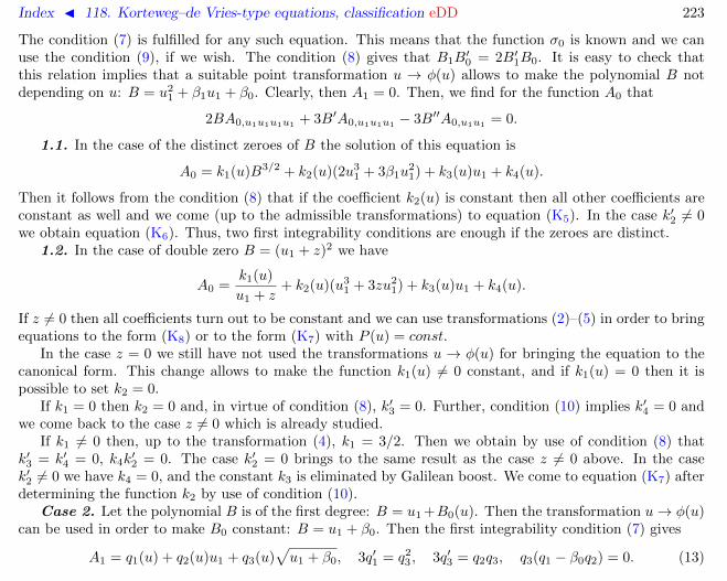
Index J 118. Korteweg–de Vries-type equations, classification eDD 223

The condition (7) is fulfilled for any such equation. This means that the function σ0 is known and we canuse the condition (9), if we wish. The condition (8) gives that B1B

′0 = 2B′1B0. It is easy to check that

this relation implies that a suitable point transformation u → φ(u) allows to make the polynomial B notdepending on u: B = u2

1 + β1u1 + β0. Clearly, then A1 = 0. Then, we find for the function A0 that

2BA0,u1u1u1u1 + 3B′A0,u1u1u1 − 3B′′A0,u1u1 = 0.

1.1. In the case of the distinct zeroes of B the solution of this equation is

A0 = k1(u)B3/2 + k2(u)(2u31 + 3β1u

21) + k3(u)u1 + k4(u).

Then it follows from the condition (8) that if the coefficient k2(u) is constant then all other coefficients areconstant as well and we come (up to the admissible transformations) to equation (K5). In the case k′2 6= 0we obtain equation (K6). Thus, two first integrability conditions are enough if the zeroes are distinct.

1.2. In the case of double zero B = (u1 + z)2 we have

A0 =k1(u)

u1 + z+ k2(u)(u3

1 + 3zu21) + k3(u)u1 + k4(u).

If z 6= 0 then all coefficients turn out to be constant and we can use transformations (2)–(5) in order to bringequations to the form (K8) or to the form (K7) with P (u) = const.

In the case z = 0 we still have not used the transformations u → φ(u) for bringing the equation to thecanonical form. This change allows to make the function k1(u) 6= 0 constant, and if k1(u) = 0 then it ispossible to set k2 = 0.

If k1 = 0 then k2 = 0 and, in virtue of condition (8), k′3 = 0. Further, condition (10) implies k′4 = 0 andwe come back to the case z 6= 0 which is already studied.

If k1 6= 0 then, up to the transformation (4), k1 = 3/2. Then we obtain by use of condition (8) thatk′3 = k′4 = 0, k4k

′2 = 0. The case k′2 = 0 brings to the same result as the case z 6= 0 above. In the case

k′2 6= 0 we have k4 = 0, and the constant k3 is eliminated by Galilean boost. We come to equation (K7) afterdetermining the function k2 by use of condition (10).

Case 2. Let the polynomial B is of the first degree: B = u1 +B0(u). Then the transformation u→ φ(u)can be used in order to make B0 constant: B = u1 + β0. Then the first integrability condition (7) gives

A1 = q1(u) + q2(u)u1 + q3(u)√u1 + β0, 3q′1 = q2

3 , 3q′3 = q2q3, q3(q1 − β0q2) = 0. (13)

Index J 118. Korteweg–de Vries-type equations, classification eDD 224

2.1. Consider the case q3 = 0 first. We have A1 = c0 + q2(u)u1 and the condition (7) is fulfilled.2.1.a. If β0 = 0 then the use of suitable change u→ φ(u) allows to set q2(u) = 0. Then the conditions

(8) and (9) proves that c0 = 0 and

A0 = c1u3/21 + c2u

21 + c3u1 + c4u+ c5,

moreover c1c4 = 0. The condition (10) gives only one additional constraint c2c4 = 0.If c4 = 0 then we come to equation (K9) and otherwise to equation (K10), up to transformations (2)–(6).2.1.b. If β0 6= 0 then it is easy to find, by use of (8) and (9), that the r.h.s. of equation does not depend

on u. Then the transformation u→ u− β0x allows to set the constant β0 to zero and to reduce this case tothe previous one.

2.2. If q3 6= 0 then equations (13) imply β0 6= 0. The use of the scaling and shift of u allows to obtainfrom (13): β0 = 1, q1 = q2 = −3 cothu, q3 = 3 sinh−1 u or β0 = 1, q1 = q2 = −3, q3 = 0. Then the conditions(7) and (8) allow to determine A0 and we come to equations (K11), (K12).

Case 3. Let B is of zero degree, then A2 = 0. The integrability condition (7) gives A1 = q(u) + p(u)u1.The use of the transformation u→ φ(u) allows to set p(u) = 0. The condition (8) implies

A0 = p1(u) + p2(u)u1 + p3(u)u21 + cu3

1, qc = qp′3 = 0.

The further analysis depends essentially on the function A1 = q(u).3.1. If q = 0 then ρ0 = 0 and condition (8) gives, in particular, relations p′2p1 = p′2p3 = 0. If p′2 6= 0

then condition (7) leads either to equation (K4) (at c 6= 0) or to (K1) or to (K2). If p′2 = 0 then we obtain,using additionally the conditions (9) and (10), the equation is either linear or all pi are constant. Further,the transformations (2)–(6) bring either to (K3) or to (K4) at c1 = c2 = 0.

3.2. If q 6= 0 then we obtain, taking into account the relations c = p′3 = 0 and with the use of condition(7) that q = c1 +c2u+c3u

2, q′p1 = 0. The further analysis is not difficult and the use of all four integrabilityconditions proves that equation coincides with one of the equations (K12), (K13), up to the transformations(2)–(6).

Index J 118. Korteweg–de Vries-type equations, classification eDD 225

References

[1] S.I. Svinolupov, V.V. Sokolov. On evolution equations with nontrivial conservation laws. Funct. Anal. Appl.16:4 (1982) 86–87.

[2] S.I. Svinolupov, V.V. Sokolov. On the conservation laws for equations with nontrivial Lie–Backlund algebra. pp.53-67 in “Integrable system”, ed. A.B. Shabat, Ufa, 1982. [in Russian]

[3] H.H. Chen, Y.C. Lee, C.S. Liu. Integrability of nonlinear Hamiltonian systems by inverse scattering method.Physica Scr. 20 (1979) 490–492.

[4] A.G. Meshkov. Necessary conditions of the integrability. Inverse Problems 10 (1994) 635–653.

Index J 119. Korteweg–de Vries-type equations, substitutions eDD 226

119 Korteweg–de Vries-type equations, substitutions

Author: V.E. Adler, 2007

1. Equations related to KdV

2. Equations related to mKdV

Notations:

ã in the substitution marked A→ B the tilded variables correspond to equation B;

ã therefore, in the sequence A → B → C the variables corresponding to B go with tilde in the firstsubstitution and without tilde in the second one;

ã for short, the dummy n in the lattice indices . . . , n− 1, n, n+ 1, . . . is omitted;

ã the letters α, β, γ are reserved for the parameters of Backlund transformations. They are always assumedto be dependent on n.

Any integrable KdV-type equation ut = uxxx+f(uxx, ux, u) is related by a differential substitution eitherto the Krichever–Novikov equation or to the KdV equation or to the linear equation [1]. While the firstcase may be considered generic, the second one is most complicated from the point of view of diversity ofcontained equations. Famous Miura transformation [2] relates KdV with the modified KdV equation.Another very important persons in the zoo are so-called exponential and elliptical Calogero–Degasperisequations (exp-CD and ℘-CD) related to mKdV by further Miura-type substitutions.

The full picture is presented below. It contains also substitutions for the corresponding dressing chains,since discrete and continuous substitutions are closely related [3, 4]. It should be noted that mKdV equationadmits two essentially different Backlund transformations. First one is inherited from BT for KdV; itcorresponds to zero curvature representation related to the Schrodinger operator and to the minus sign ofnonlinear term in mKdV. Second one corresponds to the Dirac operator, and it handles nonlinearity of anysign. Analogously, exp-CD admits three different BT, two inherited from KdV and mKdV and one for itsown.

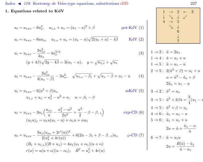
Index J 119. Korteweg–de Vries-type equations, substitutions eDD 227

1. Equations related to KdV

ut = uxxx − 6u2x, u1,x + ux = (u1 − u)2 + β pot-KdV (1)

ut = uxxx − 6uux, u1,x + ux = (u1 − u)√

2(u1 + u)− 4β KdV (2)

ut = uxxx −3u2

xx

4ux− 4u3/2

x (3)

(y + 4β)√

2y − 4β = 3(u1 − u), y =√u1,x +

√ux

ut = uxxx −3u2

xx

4(ux − β)− 3u2

x,√u1,x − β1 +

√ux − β = u1 − u (4)

ut = uxxx − 6(u2 + β)ux mKdV (5)

u1,x + ux = u21 − u2 + α, α = β1 − β

ut = uxxx − 3ux

(uxxu− u2

x − α2

2u2+u2

2− β − β−1

)exp-CD (6)

(u1u)x = u1u(u1 − u) + α1u+ αu1

ut = uxxx −3ux(uxx + 2r′(u))2

2(u2x + 4r(u))

+ 6(2u− β1 + β − β−1)ux ℘-CD (7)

(R1 + u1,x)(R+ ux) = 4u1(u1 + α1)(u+ α)

r(u) = u(u+ α)(u− α1), R2 = u2x + 4r(u)

1 → 2 ← 3↓ ↓ 4 → 5 ↓

6↓7

1→ 2 : u = 2ux

1→ 4 : u = u1 + u

1→ 5 : u = u1 − u2→ 5 : 2(u2 + β) = u1 + u

u = u2 − ux + β

2ux = u1 − u

3→ 2 : u2 = ux

3→ 5 : u3 + 3βu =3

4(u1 − u)

4→ 5 : u2 + β = ux

4→ 6 : u1 = u1 − u5→ 6 : u1 = u1 + u

2u = u+ux − αu

6→ 7 : u = u1u

2u =R(u)− uxu− α1

Index J 119. Korteweg–de Vries-type equations, substitutions eDD 228

2. Equations related to mKdV

ut = uxxx −3u2

xx

2ux, u1,xux = (u1 − βu)2 Schwarz-KdV (1)

ut = uxxx − 2u3x, u1,x + ux = eu1−u − βeu−u1 (2)

ut = uxxx − 6u2ux, u1,x + ux = (u1 − u)√

(u1 + u)2 + 4βmKdV (3)

ut = uxxx −3u2

xx

4ux− 3u2

x, (√u1,x +

√ux)2 = (u1 − u)2 − 4β (4)

ut = uxxx −3uxu

2xx

2(u2x + β)

− 2u3x (5)

(u1,x +√u2

1,x + β1)(ux +√u2x + β) = e2(u1−u)

ut = uxxx −3uxuxxu

+3u3

x

2u2− 3

2

(u− β

u

)2

ux exp-CD (6)

(u1u)x = u1u(u1 − u)− β1u+ βu1

ut = uxxx −3ux(uxx + 2r′(u))2

2(u2x + 4r(u))

+ 6(2u+ β + β−1)ux ℘-CD (7)

(R1 + u1,x)(R+ ux) = 4u1(u1 + β)(u+ β−1)

r(u) = u(u+ β)(u+ β−1), R2 = u2x + 4r(u)

1 → 2 → 3 ← 4 ↓ ↓

5 → 6 ↓

7

1→ 2 : e2u = ux

1→ 5 : 2u = log(u1 − βu)

2→ 3 : u = ux

2→ 5 : 2u = u1 + u

2u = 2u− log(ux +√u2x + β)

2→ 6 : u = eu1−u

3→ 6 : u− β/u = u1 + u

2u = u− (ux + β)/u

4→ 3 : u2 = ux

4→ 6 : u+ β/u = u1 − u5→ 6 : u− β/u = 2ux

5→ 7 : u1 = e2(u1−u)

6→ 7 : u1 = u1u

2u =R(u) + uxu+ β−1

Index J 119. Korteweg–de Vries-type equations, substitutions eDD 229

References

[1] S.I. Svinolupov, V.V. Sokolov, R.I. Yamilov. Backlund transformations for integrable evolution equations. Sov.Math. Dokl. 28 (1983) 165–168.

[2] R.M. Miura. Korteveg-de Vries equation and generalizations. I. A remarkable explicit nonlinear transformation.J. Math. Phys. 9:8 (1968) 1202–1203.

[3] R.I. Yamilov. On the construction of Miura type transformations by others of this kind. Phys. Lett. A 173:1(1993) 53–57.

[4] R.I. Yamilov. Construction scheme for discrete Miura transformations. J. Phys. A 27:20 (1994) 6839–6851.

Index J 120. Korteweg–de Vries-type equations, 5-th order eDD 230

120 Korteweg–de Vries-type equations, 5-th order

Author: V.V. Sokolov, 04.06.2008

1. Polynomial and exponential equations2. Rational and elliptic equations

The integrable equations of the 5-th order had been classified only in the constant separant case

ut = u5 + F (u4, u3, u2, u1, u). (1)

The complete list can be found in [1]. Here we present only the most important equations.The equations (3)–(10) in the list below appeared in [2, 3, 4, 5, 6]. The rest of the list appeared in [1]

for the first time (note that there was a misprint in the form of eq. (13)).The classification is based on the analysis of the necessary integrability conditions. At the first steps, it

can be proved that any equation (1) possessing higher conservation laws is of the form

ut = u5 +A1u2u4 +A2u4 +A3u23 +A4u

22u3 +A5u2u3 +A6u3

+A7u42 +A8u

32 +A9u

22 +A10u2 +A11, Ai = Ai(u, u1).

The further analysis splits in many subcases and may be very lengthy in the most degenerate ones. Forexample, the equation [7] ut = u5 + uu1 is not integrable but satisfies 10 first integrability conditions.

1. Polynomial and exponential equations

KdV eq. (118.K1) symmetry ut = u5 + 10uu3 + 20u1u2 + 30u2u1, (2)

Sawada–Kotera eq. ut = u5 + 5uu3 + 5u1u2 + 5u2u1, (3)

Kaup–Kupershmidt eq. ut = u5 + 5uu3 +25

2u1u2 + 5u2u1, (4)

ut = u5 + 5u1u3 +5

3u3

1, (5)

Index J 120. Korteweg–de Vries-type equations, 5-th order eDD 231

ut = u5 + 5u1u3 +15

4u2

2 +5

3u3

1, (6)

[2, 3, 4] ut = u5 + 5(u1 − u2)u3 + 5u22 − 20uu1u2 − 5u3

1 + 5u4u1, (7)

ut = u5 + 5(u2 − u21)u3 − 5u1u

22 + u5

1, (8)

[5] ut = u5 + 5(u2 − u21 + λ1e

2u − λ22e−4u)u3 − 5u1u

22

+ 15(λ1e2u + 4λ2

2e−4u)u1u2 + u5

1 − 90λ22e−4uu3

1

+ 5(λ1e2u − λ2

2e−4u)2u1, (9)

[6] ut = u5 + 5(u2 − u21 − λ2

1e2u + λ2e

−u)u3 − 5u1u22

− 15λ21e

2uu1u2 + u51 + 5(−λ2

1e2u + λ2e

−u)2u1. (10)

Substitutions:

(5)→ (3) : u1 = u; (9)→ (4) : 2u2 − u21 ± 6λ2e

−2uu1 + λ1e2u − λ2

2e−4u = u;

(6)→ (4) : u1 = u; (10)→ (3) : −u2 − u21 ± 3λ1e

uu1 − λ21e

2u + λ2e−u = u;

(7)→ (3) : −u1 − u2 = u; (9)|λ1=−λ2,λ2=0 = (10)|λ1=λ,λ2=0;(7)→ (4) : 2u1 − u2 = u; (9)|λ1=λ2=0 = (10)|λ1=λ2=0 = (8).(8)→ (7) : u1 = u;

2. Rational and elliptic equations

ut = u5 −5

u1u2u4 +

5

u21

u22u3 + 5

(µ1

u1+ µ2u

21

)u3 − 5

(µ1

u21

+ µ2u1

)u2

2 − 5µ2

1

u1+ 5µ1µ2u

21 + µ2

2u51, (11)

ut = u5 −5

u1u2u4 −

15

4u1u2

3 +65

4u21

u22u3 + 5

(µ1

u1+ µ2u

21

)u3

− 135

16u31

u42 − 5

(7µ1

4u21

− µ2u1

2

)u2

2 − 5µ2

1

u1+ 5µ1µ2u

21 + µ2

2u51, (12)

Index J 120. Korteweg–de Vries-type equations, 5-th order eDD 232

ut = u5 −5

2u1u2u4 −

5

4u1u2

3 +5

u21

u22u3 +

5u−1/21

2u2u3 + 5(u1 − 2µu

1/21 + µ2)u3 −

35

16u31

u42

− 5u−3/21

3u3

2 + 5(µu−1/21 − 3µ2

4u1− 1

4

)u2

2 +5u3

1

3− 8µu

5/21 + 15µ2u2

1 −40µ3u

3/21

3+ 5µ4u1, (13)

ut = u5 −15(R5 + 2R2)

2(R3 − 1)2u2u4 −

45R2

4(R3 − 1)2u2

3 +45(R10 + 22R7 + 13R4)

4(R3 − 1)4u2

2u3 + 5µR2u3

− 3645(2R12 + 4R9 +R6)

16(R3 − 1)6u4

2 −15µ(2R7 + 7R4)

4(R3 − 1)2)u2

2 +2µ2

3R5 − 5µ2

3R2, (14)

ut = u5 −15(R5 + 2R2)

2(R3 − 1)2u2u4 −

45R2

4(R3 − 1)2u2

3 +45(R10 + 22R7 + 13R4)

4(R3 − 1)4u2

2u3

− 3645(2R12 + 4R9 +R6)

16(R3 − 1)6u4

2 − 5Ω5R6 + 2R3 + 2

9R4u3 + 5Ω

10R9 + 39R6 + 36R3 − 4

12R2(R3 − 1)2u2

2

− 5Ω′10R9 − 3R6 + 12R3 + 8

54R6u2 − 5Ω2 14R9 + 39R6 + 24R3 + 4

243R10(R3 − 1)2. (15)

In (14), (15) R = R(u1) is defined as a solution of the algebraic equation

2R3 − 3u1R2 + 1 = 0,

and Ω(u) is any non-constant solution of

Ω′2 = 4Ω3 + c.

Substitutions:(11)|µ1=λ2,µ2=−λ2

1→ (10) : log u1 = u;

(12)|µ1=λ1,µ2=−λ22→ (9) : − 1

2 log u1 = u;

(13)→ (7) :√u1 − µ = u;

(14)→ (9)|λ2=0,λ1=µ : logR(u1) = u;(15)|c=−108λ2

1λ22→ (9) : A(u) + logR(u1) = u,

Index J 120. Korteweg–de Vries-type equations, 5-th order eDD 233

where A(u) is a non-constant solution of the equation

A′2 = λ22 exp(−4A)− λ1 exp(2A).

References

[1] A.V. Mikhailov, A.B. Shabat, V.V. Sokolov. The symmetry approach to classification of integrable equations.In: What is Integrability? (V.E. Zakharov ed). Springer-Verlag, 1991, pp. 115–184.

[2] A.P. Fordy, J.D. Gibbons. Some remarkable nonlinear transformations. Phys. Lett. A 75:5 (1980) 325.

[3] V.V. Sokolov, A.B. Shabat. (1980)

[4] V.G. Drinfeld, V.V. Sokolov. Lie algebras and equations of Korteweg-de Vries type. J. Soviet Math. 30 (1985)1975–2036.

[5] V.G. Drinfeld, S.I. Svinolupov, V.V. Sokolov. Classification of fifth order evolution equations with infinite seriesof conservation laws. Dokl. Akad. Nauk Ukr.SSR 10 A (1985) 8–10.

[6] Fujimoto, Watanabe (1983)

[7] Kiyotsugu, Toshio. J. Phys. Soc. Japan 50:2 (1981) 361–362.

Index J 121. Krichever–Novikov equation eDD 234

121 Krichever–Novikov equation

ut = uxxx −3

2ux(u2xx − r(u)), r = r4u

4 + · · ·+ r0 (1)

ã Introduced in [1].

ã This is the only integrable equations of the form ut = uxxx + f(uxx, ux, u) which is not related via adifferential substitution to KdV equation or linear equation [2]. The Hamiltonian structure and recursionoperator were studied in [3, 4].

ã Backlund transformation [5]:

uxvx = h(u, v), h(u, v) = h(v, u), huuu = 0, r(u) = h2v − 2hhvv.

For example, r(u) = 4u3 − g2u− g3 corresponds to

h =1

A((uv + αu+ αv + g2/4)2 − (u+ v + α)(4αuv − g3)), A2 = r(α)

where µ is the parameter of BT.

ã Nonlinear superposition principle [5] is equivalent to the (Q4) quad-equation.

ã Zero curvature representation Ut = Vx + [V,U ]:

U =1

ux

(b c−a −b

), V = −2Uxx + 2[Ux, U ]− 3

(uxxxux− 3u2

xx

2u2x

+r(u)

6u2x

)U

where a, b, c are defined by h = a(u)v2 + 2b(u)v + c(u).

References

[1] I.M. Krichever, S.P. Novikov. Holomorphic bundles over algebraic curves and nonlinear equations. Russ. Math.Surveys 35:6 (1980) 53–79.

Index J 121. Krichever–Novikov equation eDD 235

[2] S.I. Svinolupov, V.V. Sokolov, R.I. Yamilov. Backlund transformations for integrable evolution equations. Sov.Math. Dokl. 28 (1983) 165–168.

[3] V.V. Sokolov. On the Hamiltonian structure of Krichever–Novikov equation. Dokl. Akad. Nauk SSSR 277:1(1984) 48–50.

[4] O.I. Mokhov. Canonical Hamiltonian representation of the Krichever–Novikov equation. Math. Notes 50 (1991)939–945.

[5] V.E. Adler. Backlund transformation for the Krichever–Novikov equation. Int. Math. Res. Notices (1998) 1–4.

Index J 122. Kupershmidt lattice dD∆ 236

122 Kupershmidt lattice

un,t = un+1,x + u0un,x + αnunu0,x, n = 0, 1, 2, . . .

ã Dispersionless Lax pair Dt(L) = ApLx −AxLp:

A =pα+1

α+ 1+ u0p, L = pα + u0 + u1p

−α + u2p−2α + . . .

References

[1] B.A. Kupershmidt. Deformations of integrable systems. Proc. Roy. Irish Acad. Sect. A 83:1 (1983) 45–74.

Index J 123. Kuramoto–Sivashinsky equation eDD 237

123 Kuramoto–Sivashinsky equation

ut = uxxxx + µuxx + uux (1)

ã Introduced in [4]. This equation describes, in particular, the flame propagation.

ã This equation is nonintegrable. In general, its solutions demonstrate chaotic behaviour. An exactkink-like solution [4] is:

u = 120v3 + 60( µ

19− 2k2

)v − c, v = k tanh k(x− x0 − ct), 76k2 = 11µ or 76k2 = −µ.

-20 -10 10 20x

-1.5

-1

-0.5

0.5

1

1.5

u

-20 -10 10 20x

-0.3

-0.2

-0.1

0.1

0.2

0.3

u

µ = 1, k2 = 11/76; µ = −1, k2 = 1/76; (c = 0, t = 0, x0 = 0).

Index J 123. Kuramoto–Sivashinsky equation eDD 238

References

[1] G.I. Sivashinsky. Weak turbulence in periodic flows. Physica D 17:2 (1985) 243–255.

[2] V.S. L’vov, V.V. Lebedev, M. Paton, I. Procaccia. Proof of scale invariant solutions in the Kardar–Parisi–Zhangand Kuramoto–Sivashinsky equations in 1 + 1 dimensions: analytical and numerical results. Nonlinearity 6(1993) 25–47.

[3] R. Conte, M. Musette. Painleve analysis and Backlund transformation in the Kuramoto–Sivashinsky equation.J. Phys. A 22:2 (1989) 169–177.

[4] Y. Kuramoto, T. Tsuzuki. Persistent propagation of concentration waves in dissipative media far from thermalequilibrium. Progr. Theor. Phys. 55 (1976) 356–369.

Index J 124. Lagrange top D 239

124 Lagrange top

m = apᵀ − paᵀ, a = ma, m ∈ so(d), a, p ∈ Rd, p = const

This is the rest frame description of the motion in the gravity field of a d-dimensional axially symmetricrigid body with the fixed point on the axis of symmetry.

References

[1] Yu.B. Suris. The problem of integrable discretization: Hamiltonian approach. Basel: Birkhauser, 2003.

Index J 125. Lagrange top discrete ∆ 240

125 Lagrange top discrete

mn+1 = mn + anpᵀ − paᵀn, an+1 = (2I +mn)(2I −mn)−1an, mn ∈ so(d), an, p ∈ Rd, p = const

References

[1] Yu.B. Suris. The problem of integrable discretization: Hamiltonian approach. Basel: Birkhauser, 2003.

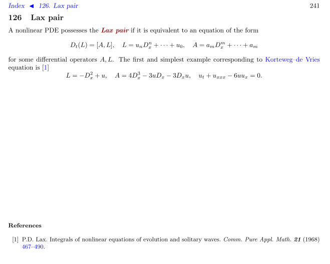
Index J 126. Lax pair 241

126 Lax pair

A nonlinear PDE possesses the Lax pair if it is equivalent to an equation of the form

Dt(L) = [A,L], L = unDnx + · · ·+ u0, A = amD

mx + · · ·+ am

for some differential operators A,L. The first and simplest example corresponding to Korteweg–de Vriesequation is [1]

L = −D2x + u, A = 4D3

x − 3uDx − 3Dxu, ut + uxxx − 6uux = 0.

References

[1] P.D. Lax. Integrals of nonlinear equations of evolution and solitary waves. Comm. Pure Appl. Math. 21 (1968)467–490.

Index J 127. Lax pair dispersionless 242

127 Lax pair dispersionless

A nonlinear PDE possesses the dispersionless Lax pair if it is equivalent to an equation of the form

Dt(L) = A,L = ApLx −AxLp, L = L(x, t; p), A = A(x, t; p)

for the coefficients of the functions L and A power expansions over parameter p.

References

[1] V.E. Zakharov. Benney’s equations and quasi-classical approximation in the inverse problem method. Funct.Anal. Appl. 14:2 (1980) 89–98.

[2] V.E. Zakharov. On the Benney’s equations. Physica D 3 (1981) 193–200.

Index J 128. Landau–Lifshitz equation eDD 243

128 Landau–Lifshitz equation

St = [S, Sxx + JS], S ∈ R3, 〈S, S〉 = 1, J = diag(J1, J2, J3), J1 + J2 + J3 = 0 (1)

ã The higher symmetry:

St3 =(Sxx +

3

2〈Sx, Sx〉S

)x− 3

2〈S, JS〉Sx.

ã The mater-symmetry [2] is local:

Sτ = [s, x(Sxx + JS) + Sx] = xSt + [S, Sx].

ã The stereographic projection

S =1

1 + zz(z + z, i(z − z), 1− zz) (2)

brings (1) to the form

izt = zxx −2z(z2

x + r)

1 + zz+

1

2r′, 4r = (J2 − J1)(z4 + 1) + 6(J1 + J2)z2.

ã In the totally anisotropic case Ji 6= Jk the zeroes of the polynomial R are distinct.

ã In the partially isotropic case one can set, without loss of generality, J1 = J2 = ± 13δ

2, r = ±δ2z2. Thesign +/− correspond to easy axis/easy plane ferromagnet.

ã The isotropic case J = 0, r = 0 correspond to Heisenberg equation.

ã The equation remains integrable also for arbitrary 4-th order polynomial r. The complexification z → u,z → 1/v, t→ it yields the system, also known as the Landau–Lifshitz equation:

ut = u2 −2(u2

1 + r(u))

u− v+

1

2r′(u), −vt = v2 −

2(v21 + r(v))

v − u+

1

2r′(v), rv = 0. (3)

Index J 128. Landau–Lifshitz equation eDD 244

ã The higher symmetry:

ut3 = u3 − u1

(6u2 + 3r′(u)

u− v− 6(u2

1 + r(u))

(u− v)2− 1

2r′′(u)

),

vt3 = v3 − v1

(6v2 + 3r′(v)

v − u− 6(v2

1 + r(v))

(u− v)2− 1

2r′′(v)

).

ã The 2× 2 zero curvature representation contains the spectral parameter on an elliptic curve. The 4× 4representation polynomial in λ was found in [3].ã Backlund transformation is defined by Shabat–Yamilov lattice.

References

[1] L.D. Landau, E.M. Lifshitz. vol. VIII. Electrodynamics of condensed matter. Moscow, Nauka, 1982.

[2] B. Fuchssteiner. On the hierarchy of the Landau–Lifshitz equation. Physica D 13:3 (1984) 387–394.

[3] L.A. Bordag, A.B. Yanovski. Polynomial Lax pairs for the chiral O(3)-field equations and the Landau–Lifshitzequation. J. Phys. A 28:14 (1995) 4007–4013.

Index J 129. Landau–Lifshitz equation, r = ±u2 (easy axis/easy plane) eDD 245

129 Landau–Lifshitz equation, r = ±u2 (easy axis/easy plane)

ut = uxx − 2u2x − δ2u2

u− v− δ2u, −vt = vxx + 2

v2x − δ2v2

u− v− δ2v

The case δ = 0 corresponds to the Heisenberg equation.ã Backlund transformation:

un,x =2hn

un+1 − vn+1+ hn,vn+1

, vn,x =2hn−1

un−1 − vn−1− hn−1,un−1

,

hn = kn(u2n + v2

n+1)− cnunvn+1, cn =2β2

n − 2δβn + δ2

2βn − δ, kn =

βn(βn − δ)2βn − δ

ã Zero curvature representation

U =1

u− v

(λ2 (u+ v) −uvλ2 − δ2 −λ2 (u+ v)

),

V = −λU +1

(u− v)2

(−λ(uv)x + δ2

2 (u2 − v2) uxv2 + u2vx

(δ2 − λ2)(u+ v)x λ(uv)x − δ2

2 (u2 − v2)

),

Wn = h−1/2n

((λ+ cn)vn+1 − 2knun −unvn+1

λ2 − δ2 −(λ+ cn)un + 2knvn+1

).

Index J 130. Landau–Lifshitz equation, r = 1 eDD 246

130 Landau–Lifshitz equation, r = 1

ut = uxx − 2u2x + δ

u− v, −vt = vxx + 2

v2x + δ

u− v

The case δ = 0 corresponds to Heisenberg equation.ã Backlund transformation:

un,x =2hn

un+1 − vn+1+ hn,vn+1 , vn,x =

2hn−1

un−1 − vn−1− hn−1,un−1 , hn = βn(un − vn+1)2 +

δ

4βn

ã Zero curvature representation

U =λ

u− v

(12 (u+ v) −uv − δ

λ2

1 − 12 (u+ v)

),

V = −λU +λ

(u− v)2

(−(uv)x uxv

2 + u2vx − 2δλ (u− v) + δ

λ2 (u+ v)x−(u+ v)x (uv)x

),

Wn = h−1/2n

(−λvn+1 + 2βn(un − vn+1) λunvn+1 + δ

λ + δ2βn

−λ λun + 2βn(un − vn+1)

).

Index J 131. Landau–Lifshitz equation, r = 0, Heisenberg equation eDD 247

131 Landau–Lifshitz equation, r = 0, Heisenberg equation

St = [S, Sxx], S ∈ R3, 〈S, S〉 = 1

ã Master-symmetry:

Sτ0 = xSx,

Sτ1 = x[S, Sxx] + [S, Sx],

Sτ2 = x(Sxxx + 2〈Sx, Sx〉Sx + 2〈Sx, Sxx〉S) + 2Sxx + 3〈Sx, Sx〉S + SxD−1x (〈Sx, Sx〉)

ã sl2 version:2St = [S, Sxx], S ∈ sl2, S2 = 1.

ã Zero curvature representation:U = λS, V = 2λ2S + λSSx.

ã Polynomial parametrization:

S =

(1− pq uq(2− pq) pq − 1

)⇒pt = p2 + (p2q1)xqt = −q2 + pq2

1

ã Rational parametrization given by the stereographic projection (128.2) brings to

ut = uxx −2u2

x

u− v, −vt = vxx +

2v2x

u− vã Backlund transformation:

un,x =βn(vn+1 − un)(un − un+1)

vn+1 − un+1, vn,x =

βn−1(vn−1 − vn)(vn − un−1)

vn−1 − un−1

ã Zero curvature representation

U =λ

u− v

(12 (u+ v) −uv

1 − 12 (u+ v)

), V = −λU +

λ

(u− v)2

(−(uv)x uxv

2 + u2vx−ux − vx (uv)x

),

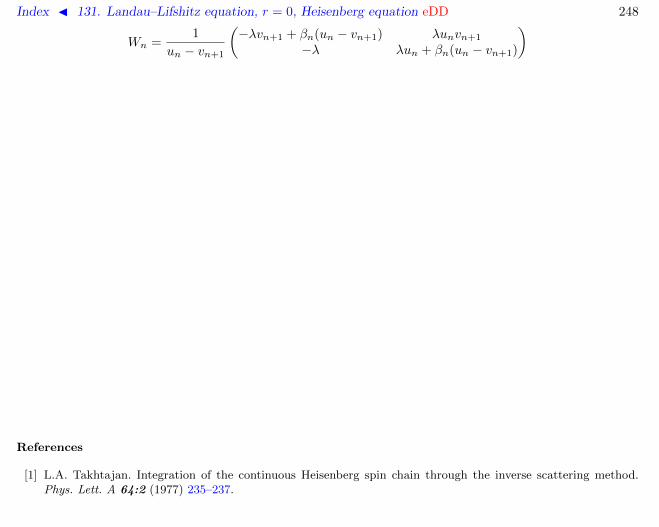
Index J 131. Landau–Lifshitz equation, r = 0, Heisenberg equation eDD 248

Wn =1

un − vn+1

(−λvn+1 + βn(un − vn+1) λunvn+1

−λ λun + βn(un − vn+1)

)

References

[1] L.A. Takhtajan. Integration of the continuous Heisenberg spin chain through the inverse scattering method.Phys. Lett. A 64:2 (1977) 235–237.

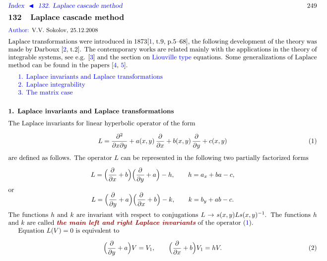
Index J 132. Laplace cascade method 249

132 Laplace cascade method

Author: V.V. Sokolov, 25.12.2008

Laplace transformations were introduced in 1873[1, t.9, p.5–68], the following development of the theory wasmade by Darboux [2, t.2]. The contemporary works are related mainly with the applications in the theory ofintegrable systems, see e.g. [3] and the section on Liouville type equations. Some generalizations of Laplacemethod can be found in the papers [4, 5].

1. Laplace invariants and Laplace transformations2. Laplace integrability3. The matrix case

1. Laplace invariants and Laplace transformations

The Laplace invariants for linear hyperbolic operator of the form

L =∂2

∂x∂y+ a(x, y)

∂

∂x+ b(x, y)

∂

∂y+ c(x, y) (1)

are defined as follows. The operator L can be represented in the following two partially factorized forms

L =( ∂∂x

+ b)( ∂

∂y+ a)− h, h = ax + ba− c,

or

L =( ∂∂y

+ a)( ∂

∂x+ b)− k, k = by + ab− c.

The functions h and k are invariant with respect to conjugations L → s(x, y)Ls(x, y)−1. The functions hand k are called the main left and right Laplace invariants of the operator (1).

Equation L(V ) = 0 is equivalent to( ∂∂y

+ a)V = V1,

( ∂∂x

+ b)V1 = hV. (2)

Index J 132. Laplace cascade method 250

If h 6= 0, then V1 satisfies a new hyperbolic equation( ∂2

∂x∂y+ a1(x, y)

∂

∂x+ b1(x, y)

∂

∂y+ c1(x, y)

)V1 = L1(V1) = 0,

where

a1 = a− (log h)y, b1 = b, c1 = a1b1 + by − h.

In it easy to see that

L1 =( ∂∂y

+ a1

)( ∂∂x

+ b)− h =

( ∂∂x

+ b)( ∂

∂y+ a1

)− h1,

where

h1 = a1,x − by + h.

The main right Laplace invariant k1 of L1 coincides with h. Notice that( ∂∂y

+ a1

)L = L1

( ∂∂y

+ a).

We say that operator L1 is obtained as the result of Laplace y-transformation of the operator L. Itfollows from (2) that any solution of the equation L(V ) = 0 produces a solution of the equation L1(V1) = 0and vice versa.

If h1 6= 0, we can apply the same procedure to the operator L1 and so on. As the result we obtain achain of operators

Li =( ∂∂x

+ b)( ∂

∂y+ ai

)− hi =

( ∂∂y

+ ai

)( ∂∂x

+ b)− hi−1, i ∈ N, (3)

where ( ∂∂y

+ ai

)Li−1 = Li

( ∂∂y

+ ai−1

).

Index J 132. Laplace cascade method 251

The coefficients ai and the Laplace invariants of these operators are related by the formulas

ai = ai−1 − (log hi−1)y, hi = ai,x − by + hi−1. (4)

Here a0 = a, h0 = h. It follows from these formulas that

hi = 2hi−1 − hi−2 − (log hi−1)xy, (5)

and ki = hi−1. The chain (5) is nothing but the famous integrable Toda lattice.If k 6= 0, then starting from the operator L, we can define another chain of operators L1, L2, . . . by the

relations ( ∂∂x

+ bi

)Li−1 = Li

( ∂∂x

+ bi−1

).

For this chain we have

bi = bi−1 − (log ki−1)x, ai = a, ki = bi,y − ax + ki−1,

where ki is the main Laplace invariant playing the same role for Li as k for L; another invariant coincideswith ki−1. If we denote h−1 = k and h−i−1 = ki, i = 1, 2, . . . , then we get the complete set of the Laplaceinvariants hi, i ∈ Z. It can be easily verified that all Laplace invariants satisfy (5).

The operator

Lᵀ =∂2

∂x∂y− a ∂

∂x− b ∂

∂y+ (c− ax − by)

is called adjoint to the operator L. It is not difficult to show that the Laplace invariants Hi of the operatorLᵀ is related to the Laplace invariants of L by

Hn = h−n−1, n = 0,±1,±2, . . .

2. Laplace integrability

According to (2), we have

Vi =1

hi

( ∂∂x

+ b)Vi+1

Index J 132. Laplace cascade method 252

and therefore

V =1

h

( ∂∂x

+ b) 1

h1

( ∂∂x

+ b)· · · 1

hp−1

( ∂∂x

+ b)Vp,

where Li(Vi) = 0. Since∂

∂x+ b = e−∫ bdx

∂

∂xe∫ bdx,

hence the latter formula can be rewritten as

V e∫ bdx =1

h

∂

∂x

1

h1

∂

∂x· · · 1

hp−1

∂

∂x

(Vpe∫ bdx) . (6)

Analogously,

V e∫ ady =1

k

∂

∂y

1

k1

∂

∂y· · · 1

kq−1

∂

∂y

(V−qe

∫ ady) ,where Li(V−i) = 0.

If for some p we have hp ≡ 0, then the chain of operators Li is terminated. In this case the equationLp(Vp) = 0 can be easily solved. It follows from (3) that( ∂

∂y+ ap

)Vp = Y (y)e−∫ bdx

or

Vp = e−∫ apdy(X(x) +

∫Y (y)e∫(apdy−bdx)dy

),

where X and Y are arbitrary functions of variables x and y correspondingly. Let

α = e−∫ apdy, β = e∫ apdy−bdx,

then

Vp = α(X +

∫Y βdy

).

Index J 132. Laplace cascade method 253

Substituting this to (6), we get

V = A(X +

∫Y βdy

)+A1

(X ′ +

∫Y∂β

∂xdy)

+ · · ·+Ap

(dpXdxp

+

∫Y∂pβ

∂xpdy),

where A,A1, . . . , Ap are some given functions of x and y and X(x), Y (y) are arbitrary functions. Thus thegeneral solution of the equation L(V ) = 0 can be found in quadratures by (6). Notice that this solution islocal with respect to the function X but non-local in Y .

Choosing Y = 0, we get the following special solution:

V = AX +A1X′ + · · ·+Ap

dpX

dxp. (7)

Thus, if hp = 0, then the equation L(V ) = 0 has a special solution of the form (7), where X(x) is arbitraryfunction. The converse statement is also true.

Lemma 1. Let equation L(V ) = 0 has a solution of the form (7), where function X(x) is arbitrary. Thenan integer m exists such that 0 ≤ m ≤ p and hm = 0.

The operator L is called Laplace integrable if there exist p ≥ 0 and q ≥ 0 such that hp ≡ 0 and kq ≡ 0.The concept of the Laplace integrability is crucial for the definition of so called Liouville type nonlinearhyperbolic equations (see also [6, 7] and references therein).

The general solution of the equation L(V ) = 0 with Laplace integrable operator is local in both arbitraryfunctions:

V = AX +A1X′ + · · ·+Ap

dpX

dxp+BY +B1Y

′ + · · ·+BqdqY

dyq.

It is clear that Lᵀ is Laplace integrable if and only if L is Laplace integrable.

3. The matrix case

Consider now operator (1) with coefficients a, b, c being N ×N matrices. A straightforward generalization ofall definitions to the matrix case looks as follows. The main Laplace invariants are defined by the formulas

h0 = ax + ba− c, h−1 = k0 = by + ab− c.

Index J 132. Laplace cascade method 254

Actually, only spectrum of the matrices h0, h−1 is invariant with respect to the transformations L →s(x, y)Ls(x, y)−1. However by an analogy to the scalar case, we prefer to keep the name “invariant” forthese matrices.

The matrices hi for i > 0 are recurrently determined from the following system of equations

hi,y − hiai + ai+1hi = 0, (8)

hi+1 = 2hi + (ai+1 − ai)x + [b, ai+1 − ai]− hi−1, (9)

where a0 = a. Obviously, in the scalar case these formulas coincide with the corresponding ones from section1. Suppose the matrices hi and ai for i ≤ k are already given. Then we derive ak+1 from (8) and after thatfind hk+1 from (9). However if dethk = 0, then ak+1 does not exist at all or it is defined not uniquely butup a matrix α such that αhk = 0. In the latter case, the existence and properties of next Laplace invariantsessentially depend on the choice of α. At first glance, such degenerations are very special, but in applicationsof the Laplace invariants to the Liouville type integrable systems this is a generic case.

To overcome this difficulty, we consider the products Hi = hihi−1 · · ·h1h0. The matrices Hi are calledgeneralized Laplace invariants. For the scalar case the formulas (4) are equivalent to

ai = a− (logHi−1)y, hi = ai,x − by + hi−1.

These formulas are generalized to the matrix case as follows:

Hi,y −Hia+ ai+1Hi = 0, (10)

hi+1 = ai+1,x + [b, ai+1]− by + hi, Hi+1 = hi+1Hi, (11)

and H0 = h0. To get Hi+1 we have to solve equation (10) for ai+1 and substitute the result into (11). Thegeneralized Laplace invariants Ki are defined by

Ki,x −Kib+ bi+1Ki = 0, (12)

ki+1 = bi+1,y + [a, bi+1]− ax + ki, Ki+1 = ki+1Ki, (13)

and K0 = k0.In a slightly different form the following statement was proved in [6].

Index J 132. Laplace cascade method 255

Theorem 2. The generalized Laplace invariant Hm exists and is well-defined if and only if( ∂∂y

+ a)

(kerHi) ⊂ kerHi and( ∂∂x

+ b)

(ImHi) ⊂ ImHi

for all i < m. After evident reformulation the statement is valid for the invariants Ki.

As in the scalar case, we have the following theorem.

Theorem 3 (Startsev [8]). Suppose that the Laplace invariants Hi of operator (1) with matrix coefficientsexist and are well defined for all i ≤ p and Hp = 0. Then a differential operator exists

S =

p∑j=0

Aj(x, y)∂j

∂xj,

where Aj are square matrices and det(Ap) 6= 0, such that S(f(x)) is a solution of the system L(V ) = 0 forany vector-function f(x).

Definition 4. The operator (1) with matrix coefficients is called Laplace integrable if the generalized Laplaceinvariants Hi and Ki exist, are well defined, and Hp ≡ 0, Kq ≡ 0 for some p ≥ 0, q ≥ 0.

Index J 132. Laplace cascade method 256

References

[1] P.S. Laplace. Oeuvres completes. Paris, 1893.

[2] G. Darboux. Lecons sur la theorie generale des surfaces et les applications geometriques du calcul infinitesimal.T. I-IV. 3 ed., Paris: Gauthier-Villars, 1914–1927.

[3] S.P. Tsarev. Factoring linear partial differential operators and the Darboux method for integrating nonlinearpartial differential equations. Theor. Math. Phys. 122:1 (2000) 121–133.

[4] J. Le Roux. Extensions de la methode de Laplace aux equations lineaires aux derivees partielles d’ordre superieurau second. Bull. Soc. Math. de France 27 (1899) 237–262.

[5] C. Athorne. A Z2 × R3 Toda system. Phys. Lett. A 206 (1995) 162–166.

[6] A.V. Zhiber, V.V. Sokolov. Exactly integrable hyperbolic equations of Liouville type. Russ. Math. Surveys 56:1(2001) 61–101.

[7] I.M. Anderson, M. Juras. Generalized Laplace invariants and the method of Darboux. Duke Math. J. 89:2(1997) 351–375.

[8] S.Ya. Startsev. Cascade method of Laplace integration for linear hyperbolic system of equations Math. Notes83:1 (2008) 97–106.

Index J 133. Laurent property 257

133 Laurent property

A rational mapping f : Cn → Cn satisfies the Laurent property if all its iterations fk(x) are Laurentpolynomials on the initial data x = (x1, . . . , xn), that is, the denominator of fk(x) is at most a monomial inx1, . . . , xn.

Example: Somos sequences.

Index J 134. Left-symmetric algebra 258

134 Left-symmetric algebra

Author: V.V. Sokolov, 04.07.2006

Left-symmetric algebra (A, ) is characterized by identity

As(a, b, c) = As(b, a, c),

where As denotes the associator

As(a, b, c) = (a b) c− a (b c).

This class of algebras is obviously a generalization of associative ones for which As(X,Y, Z) = 0. Anotherexample of left-symmetric algebra is given by Euclidean space equipped with the multiplication

a b = 〈a, c〉b+ 〈a, b〉c

where c is a fixed vector.The left-symmetric algebras are related with multi-field analogs of Burgers equation.

Index J 135. Levi system eDD 259

135 Levi system

pt = pxx + (p2 + 2pq + 2βp)x, qt = −qxx + (q2 + 2pq + 2βq)x

ã Introduced in [1]

ã Levi system is related to NLS system by Backlund transformation

uv = pq − qx, ux/u = p+ q + β

and to DNLS system by the differential substitution

p = bx/b− ab/2, q = −ab/2.

ã Backlund transformation:

pj,x = pj(pj+1 − pj + qj+1 − qj + βj+1 − βj), qj,x = pjqj − pj−1qj−1.

ã Hamiltonian structure for this lattice:

pj , qj = −pj , pj , qj+1 = pj , H =∑(1

2q2j + βjqj + pjqj

).

ã Nonlinear superposition principle

pk−1 = pk−1

(1− βk − βk−1

pk−1 − qk

), pk = pk

(1 +

βk − βk−1

pk−1 − qk − α

),

qk−1 = qk−1 +(βk − βk−1)qkpk−1 − qk

, qk = qk

(1− βk − βk−1

pk−1 − qk

),

βk−1 = βk, βk = βk−1

ã Zero curvature representation Ut = Vx + [V,U ], Wx = U1W −WU :

U =

(s− λ −qp λ− s

), V = 2(λ+ s)U +

(12 (p− q) q

p 12 (q − p)

)x

, 2s = p+ q + β

Index J 135. Levi system eDD 260

Wj = p−1/2j

(pj −qj+1

pj 2λ− βj+1 − qj+1

)

References

[1] D. Levi. Nonlinear differential difference equations as Backlund transformations. J. Phys. A 14:5 (1981) 1083–1098.

[2] A.V. Mikhailov, A.B. Shabat, R.I. Yamilov. The symmetry approach to classification of nonlinear equations.Complete lists of integrable systems. Russ. Math. Surveys 42:4 (1987) 1–63.

Index J 136. Lie algebra 261

136 Lie algebra

Lie algebra L is the algebra with the skew-symmetric multiplication [·, ·] : L × L → L which satisfies theJacobi identity

[a, b] = −[b, a], [a, [b, c]] + [b, [c, a]] + [c, [a, b]] = 0.

Any associative algebra A gives rise to the Lie algebra A− with respect to the product [a, b] = ab− ba. AnyLie algebra is isomorphic to a subalgebra of some A−.

Index J 137. Lie group 262

137 Lie group

The n-parametric Lie group is a smooth n-dimensional manifold G equipped with the operations of multi-plication G × G → G and taking the inverse G → G which are smooth mappings and satisfy the commongroup axioms (1).

Local Lie groups, Lie groups of transformations

Index J 138. Liouville equation hDD 263

138 Liouville equation

uxy = eu

ã This is a classical example of linearizable equation. The substitution from the linear equation

eu =2vxvyv2

= −2(log v)xy, vxy = 0

yields the formula for the general solution u = log(

2a′(x)b′(y)(a(x)+b(y))2

).

ã Alternatively, the solution can be found from two consistent ODEs

uxx −1

2u2x = c(x), uyy −

1

2u2y = k(y)

with arbitrary functions c, k. An immediate check proves that, indeed,

Dy(uxx −1

2u2x) = 0, Dx(uyy −

1

2u2y) = 0

in virtue of Liouville equation. These expressions are called y- and x-integrals respectively.

References

[1] J. Liouville. Sur l’equation aux differences partielles d2 log λ/dudv ± λ/2a2 = 0. J. Math. Pures Appl. 18:1(1853) 71–72.

Index J 139. Liouville type equations hDD 264

139 Liouville type equations

A nonlinear hyperbolic equation of the form

uxy = f(x, y, u, ux, uy)

belongs to Liouville equation type if it possesses some of the following properties:

ã its general solution is given by an explicit formula (Darboux integrability);

ã it is linearizable (C-integrability);

ã its symmetry algebra contains arbitrary functions;

ã the nontrivial integrals in both characteristics exist;

ã the sequence of its Laplace invariants is terminated by zero in both directions (Laplace integrability).

It should be stressed that although these properties are in close relation, they are not equivalent andthere exist the examples of equations which satisfy only some subset of them. Several classification resultsare known based on the analysis of these features.

References

[1] A.V. Zhiber, N.H. Ibragimov, A.B. Shabat. Liouville type equations. DAN SSSR 249:1 (1979) 26–29.

[2] A.V. Zhiber, A.B. Shabat. Nonlinear Klein–Gordon equations with nontrivial group. Dokl. Akad. Nauk SSSR247:5 (1979) 1103–1107.

[3] A.V. Zhiber, A.B. Shabat. The systems ux = p(u, v), vy = q(u, v) possessing symmetries. Dokl. Akad. NaukSSSR 277:1 (1984) 29–33.

[4] I.M. Anderson, N. Kamran. The variational bicomplex for second order scalar partial differential equations inthe plane. Duke Math. J. 87:2 (1997) 265–319.

[5] A.V. Zhiber, V.V. Sokolov. Exactly integrable hyperbolic equations of Liouville type. Russ. Math. Surveys 56:1(2001) 61–101.

Index J 140. Liouville integrability 265

140 Liouville integrability

Author: A.Ya. Maltsev, 2.10.2009

Consider the Hamiltonian system

xi = J ij∂H

∂xj= xi, H

(summation over repeated indices is assumed) on a manifold M2n with a non-degenerate Hamiltonianoperator J ij(x). This system is called integrable in the Liouville sense [1] if there exist n first integralsIν , Iν , H = 0, ν = 1, . . . , n, such that:

1) the integrals Iν are functionally independent (rank ||∂Iν/∂xi|| = n);

2) the integrals Iν commute with each other,

Iν , Iµ = 0, ν, µ = 1, . . . , n;

3) the common level surfaces Iν(x) = const, ν = 1, . . . , n are compact manifolds in M2n.

The following remarkable facts can be proved under these conditions.

Theorem 1 (Liouville). Almost all common level surfaces of the first integrals Iν(x) = const, ν = 1, . . . , nare n-dimensional tori Tn embedded in M2n. In the vicinity of every such torus the so called action-anglecoordinates (J1, . . . , Jn, θ1, . . . , θn) can be introduced such that:

1) in these coordinates the Poisson bracket has the canonical form (see Darboux theorem)

Jα, Jβ = 0, θα, θβ = 0, Jα, θβ = δαβ , α, β = 1, . . . , n;

2) on the tori Tn, the coordinates (θ1, . . . , θn) take the values 0 ≤ θα < 2π, while the coordinates(J1, . . . , Jn) are constant;

3) the Hamiltonian function H has constant values on the tori Tm and depends on the values of (J1, . . . , Jm)only: H = H(J1, . . . , Jm).

Index J 140. Liouville integrability 266

It can be easily deduced then that the tori Tn give invariant manifolds for the corresponding dynamicalsystem, such that the values of Jα remain constant, while the coordinates θα depend linearly on time withsome constant frequencies ωα(J):

θα(t) = θα0 + ωα(J)t.

The Liouville theorem gives a beautiful description of the global behavior of the trajectories of integrablesystems from the geometrical point of view. Thus, the trajectory of an integrable dynamical system givesthe irrational covering of some n-dimensional torus Tn ⊂ M2n in generic situation. It is easy to see alsothat every dynamical system defined by any Hamiltonian function H = H(J) is integrable in the Liouvillesense and has the same invariant tori Tn as the initial one. So, the integrability in Liouville sense implies infact the existence of infinite number of integrable dynamical systems which commute with each other.

The definition of the integrable system can be generalized also to the case of the Poisson structure ofconstant rank. Namely, we can say that the Hamiltonian dynamical system is integrable if all Casimirfunctions are globally defined on Mm and the restriction of the dynamical system on every common levelsurface of Casimir functions N1 = const, . . . , Nm−2n = const gives an integrable system in the Liouvillesense.

References

[1] V.I. Arnold. Mathematical Methods of Classical Mechanics. Springer: 1978, 1989.

Index J 141. Loop algebra 267

141 Loop algebra

A loop algebra is the Lie algebra of the formal Laurent series with the coefficients in some lie algebra L:

L(λ) = u0λn + u1λ

n−1 + u2λn−2 + . . . | n ∈ Z, ui ∈ L.

Loop algebras are related with several schemes of construction and solving of integrable systems, from rathersimple to more or less universal ones.

As a simplest example consider the Lax equation on L(λ) of the form

Utn = [Un, U ], U = u0 + u1/λ+ u2/λ2 + . . . , Un = (λnU)+ = u0λ

n + u1λn−1 + · · ·+ un. (1)

This gives the infinite system of equations for the coefficients

u0,t0 = 0, u0,t1 = 0, u0,t2 = 0, . . .

u1,t0 = [u0, u1], u1,t1 = [u0, u2], u1,t2 = [u0, u3], . . .

u2,t0 = [u0, u2], u2,t1 = [u0, u3] + [u1, u2], u2,t2 = [u0, u4] + [u1, u3], . . .

u3,t0 = [u0, u3], u3,t1 = [u0, u4] + [u1, u3], u3,t2 = [u0, u5] + [u1, u4] + [u2, u3], . . .

. . . . . . . . . . . .

which possesses the properties formulated in the following statement. These properties are not related withthe nature of Lie algebra L.

Statement 1. 1) The flows Dtn defined by equations (1) commute, that is Dtn(Dtm(uj)) = Dtm(Dtn(uj))for all j,m, n;

2) the identities um+1,tn = un+1,tm hold, and this makes possible to introduce the potential v ∈ Laccordingly to the formulas un = vtn−1

;3) the flow Dτ defined by equation

Uτ = [v, U ]− λ2Uλ ⇔ uk,τ = [v, uk] + (k + 1)uk+1 (2)

is the master-symmetry of the hierarchy (1):

[Dτ , Dtn ] = nDtn+1.

Index J 141. Loop algebra 268

Proof. 3) One has

[Dτ , Dtn ](U) = [Un, U ]τ − ([v, U ]− λ2Uλ)tn

= [Un,τ − vtn , U ] + [Un, [v, U ]− λ2Uλ]− [v, [Un, U ]] + λ2[Un, U ]λ

= [(λnUτ )+ − un+1 + [Un, v] + λ2Un,λ, U ]

= [−(λn+2Uλ)+ − un+1 + λ2Un,λ, U ] = n[Un+1, U ],

since

− (λn+2Uλ)+ − un+1 + λ2Un,λ = u1λn + 2u2λ

n−1 + · · ·+ (n+ 1)un+1 − un+1

+ λ2(nu0λn−1 + (n− 1)u1λ

n−2 + · · ·+ un−1) = nUn+1.

Various integrable models appear after the concrete choice of the Lie algebra.

Example 2. If L is a finite-dimensional Lie algebra then equations (1) become (1+1)-dimensional integrablesystems of NLS or N -wave types. Here the choice of the first coefficient u0 (which is a constant of motionin virtue of the equations) is of importance.

Example 3. The examples of dispersionless PDE in any dimension appear id L is an infinite-dimensional Liealgebra of the vector fields on some manifold. Let, for instance, L consists of the vector fields on the line,that is ui are just functions depending on the additional variable x and the commutator is defined by theformula [u, v] = uvx − vux (after identifying u ↔ u∂x). Clearly, in the ψ-function language this examplecorresponds to the auxiliary linear problems of the form ψtn = (λn + u1λ

n−1 + · · · + un)ψx. The choiceu0 = 1 allows to identify Dx and Dt0 . In this case equations (1) generate a (2+1)-dimensional dispersionlesshierarchy with the simplest representative (in potential form)

vxt2 − vt1t1 + vxvxt1 − vxxvt1 = 0.

More generally, let L be Lie algebra of the vector fields in RN , that is ui = (u1i , . . . , u

Ni ) and the commutator

is defined accordingly to the identification ui →∑uki ∂xk

. Again, one can assume Dt0 = Dx = Dx1without

Index J 141. Loop algebra 269

loss of generality, under the choice u0 = (1, 0, 0, . . . ). Then the vector potential v = (v1, . . . , vN ) satisfiesthe equation

vxt2 − vt1t1 + [vx, vt1 ] = 0

which contain the partial derivatives with respect to 2 +N independent variables t1, t2 and x = x1, . . . , xN .The formula (2) leads to the master-symmetries of this equation

vxT = [v, vx] + 2vt1 + t1(vt1t1 − [vx, vt1 ]).

Interesting reductions correspond to the Lie subalgebras of contact or hamiltonian vector fields. Forinstance, the choice N = 2, v = (Hp,−Hx) leads to 4D-equation

Hxt2 −Ht1t1 +Hxt1Hxp −HxxHpt1 = 0. (3)

This construction is not unique. It admits many variations depending on the definition of the elementUn in (1). In particular, these versions are related with different decompositions of Lie algebra L intosubalgebras and with the corresponding gradings in L(λ). For example, an easy exercise proves, that thechoice Un = u0λ

n + u1λn−1 + · · · + un−1λ lead to the commuting flows as well. In the case L = sl2 these

lead to Heisenberg model instead of NLS, and the algebra of Hamiltonian vector fields on the plane leads,instead of (3), to equation

Ht1t1 = Hpt1Hxt2 −Hpt2Hxt1 , (4)

which is related to Plebanski equation.

References

[1] A.C. Newell. Solitons in mathematics and physics. Philadelphia: SIAM, 1985.

Index J 142. Lorenz system eDD 270

142 Lorenz system

x = k(x− y), y = rx− y − zx, z = xy − bz.

This is a famous example of nonintegrable ODE demonstrating strange attractor.

References

[1] G.M. Zaslavsky, R.Z. Sagdeev. Introduction to nonlinear physics. Moscow, Nauka, 1988.

[2] M. Kus. Integrals of motion for the Lorenz system, J. Phys. A 16:18 (1983) L689–692.

[3] T. Sen, M. Tabor. Lie symmetries of the Lorenz model. Physica D 44:3 (1990) 313–339.

[4] N. Gupta. Integrals of motion for the Lorenz system, J. Math. Phys. 34:2 (1993) 801–804.

[5] P.G.L. Leach, G.P. Flessas. Solutions in closed form and as power series to the real Lorenz equations. J. Phys.A 34:30 (2001) 6013–6029.

Index J 143. Manakov system eDD 271

143 Manakov system

ut = uxx + 2〈u, v〉u, −vt = vxx + 2〈u, v〉v, u, v ∈ RN

This is the first and simplest multifield generalization of NLS equation.ã Backlund transformation [2, 3]:

un,x = un+1 + βnun + 〈un, vn+1〉un, −vn,x = vn−1 + βn−1vn + 〈un−1, vn〉vn. (1)

Third order symmetry:

ut3 = uxxx + 3〈u, v〉ux + 3〈ux, v〉u, vt3 = vxxx + 3〈u, v〉vx + 3〈u, vx〉v.

The quantitiesU = −2〈u, v〉, W = 2〈u, vx〉 − 2〈ux, v〉

satisfy the Kadomtsev–Petviashvili equation [4, 5, 6].

4Ut3 = Uxxx − 6UUx + 3Wt, Wx = Ut.

The quantities

Fn = −〈un, vn+1〉 − βn, Pn = 〈un, vn+1,x〉 − 〈un,x, vn+1〉+ 〈un, vn+1〉2 − β2n

yield, in virtue of (1), the Miura-type transformation [7]

Un+1 = Un + 2Fn,x, Un = F 2n − Fn,x + Pn, Pn,x = Fn,t

between KP and modified Kadomtsev–Petviashvili equation

4Ft3 = Fxxx − 6(F 2 + P )Fx + 3Pt, Px = Ft.

The variables F, P satisfy the 2D dressing chain

Fn+1,x + Fn,x = F 2n+1 − F 2

n + Pn+1 − Pn, Pn,x = Fn,t.

Index J 143. Manakov system eDD 272

References

[1] S.V. Manakov. On the theory of two-dimensional stationary self-focusing of electromagnetic waves. Sov. Phys.JETP 38:2 (1974) 248–253.

[2] A.B. Shabat, R.I. Yamilov. Symmetries of nonlinear chains. Len. Math. J. 2:2 (1991) 377–399.

[3] V.E. Adler. Nonlinear superposition formula for Jordan NLS equations. Phys. Lett. A 190 (1994) 53–58.

[4] B.G. Konopelchenko, W. Strampp. The AKNS hierarchy as symmetry constraint of the KP hierarchy. InverseProblems 7 (1991) L17–24.

[5] B.G. Konopelchenko, J. Sidorenko, W. Strampp. (1+1)-dimensional integrable systems as symmetry constraintsof (2+1)-dimensional systems. Phys. Lett. A 157:1 (1991) 17–21.

[6] Y. Cheng, Y. Li. The constraint of the Kadomtsev–Petviashvili equation and its special solutions. Phys. Lett.A 157:1 (1991) 22–26.

[7] B.G. Konopelchenko. On the general structure of nonlinear evolution equations integrable by the two-dimensionalmatrix spectral problem. Commun. Math. Phys. 87:1 (1982) 105–125.

Index J 144. Massive Thirring model hDD 273

144 Massive Thirring model

iux + v + u|v|2 = 0, ivt + u+ v|u|2 = 0

Index J 145. Master-symmetry 274

145 Master-symmetry

An evolutionary equation uτ = K(x, u, u1, . . . , um) is called master-symmetry for equation ut = F (x, u, u1, . . . , um)if the corresponding evolutionary derivatives satisfy the relation [∇F , [∇F ,∇K ]] = 0.

The notion of master-symmetry was introduced by Fokas and Fuchssteiner [1, 2, 3]. The first exampleappeared actually in [4].

The master symmetries can be introduced through the zero curvature representation with the time-dependent spectral parameters [5, 6, 7].

Master symmetries for many equations (e.g., for the KdV, NLS, and Toda chain equations) are nonlocal.However, the Landau–Lifshitz model, which is an universal equation in the NLS class, has the local mastersymmetry.

References

[1] A.S. Fokas, B. Fuchssteiner. The hierarchy of the Benjamin–Ono equation. Phys. Lett. A 86:6–7 (1981) 341–345.

[2] B. Fuchssteiner. Master symmetries, higher order time-dependent symmetries and conserved densities of non-linear evolution equations. Progr. Theor. Phys. 70:6 (1983) 1508–1522.

[3] A.S. Fokas. Symmetries and integrability. Stud. Appl. Math. 77 (1987) 253–299.

[4] N.H. Ibragimov, A.B.Shabat. Group theoretical approach to the Korteweg-de Vries equation. Dokl. Akad. NaukSSSR 244:1 (1979) 57–61.

[5] A.Yu. Orlov, E.I. Shulman. On additional symmetries of nonlinear Schrodinger equation. Theor. Math. Phys.64:2 (1985) 862–866.

[6] A.Yu. Orlov, E.I. Shulman. Additional symmetries for integrable equations and conformal algebra representation.Lett. Math. Phys. 12:3 (1986) 171–179.

[7] S.P. Burtsev, V.E. Zakharov, A.V. Mikhailov. Inverse scattering method with the variable spectral parameter.Theor. Math. Phys. 70:3 (1987) 227–240.

Index J 146. Maxwell–Bloch equation DD 275

146 Maxwell–Bloch equation

Reduced Maxwell–Bloch equation:

Et = V, Vx = ωR+ EQ, Qx = −EV, Rx = −ωV

Index J 147. Melnikov system eDDD 276

147 Melnikov system

ut = uxxx + 6uux + 3vyy − 〈φ, ψ〉x, vx = u, φy = φxx + uφ, −ψy = ψxx + uψ (1)

This multifield generalization [1] of KP equation belongs to the type called equations which self-consistentsources. Equation for the vector ψ coincide with equation of auxiliary linear problem for KP equation andφ satisfies the conjugated equation. The choice of the next flow leads to the system

ut = uxxx + 6uux + 3vyy + 6(〈φ, ψxx〉 − 〈φxx, ψ〉+ 〈φ, ψ〉y), vx = u,

4φt = 4φxxx + 6uφx + (3ux − v − 2〈φ, ψ〉)φ, 4ψt = 4ψxxx + 6uψx + (3ux + v + 2〈φ, ψ〉)ψ,(2)

which also was introduced in [1]. The similar equation were studied further in [2, 3, 4, 5, 6]. The stationaryflow of the system (1) is called Melnikov system as well [7].

References

[1] V.K. Mel’nikov. On equations for wave interactions. Lett. Math. Phys. 7:2 (1983) 129–136.

[2] V.K. Mel’nikov. A direct method for deriving a multisoliton solution for the problem of interaction of waves onthe x, y plane. Commun. Math. Phys. 112:4 (1987) 639–652.

[3] V.K. Mel’nikov. Integration method of the Korteweg-de Vries equation with a self-consistent source. Phys. Lett.A 133:9 (1988) 493–496.

[4] V.K. Mel’nikov. Interaction of solitary waves in the system described by the Kadomtsev–Petviashvili equationwith a self-consistent source. Commun. Math. Phys. 126:1 (1989) 201-215.

[5] V.K. Mel’nikov. Integration of the Korteweg-de Vries equation with a source. Inverse Problems 6 (1990) 233–246.

[6] V.K. Mel’nikov. Integration of the nonlinear Schrodinger equation with a source. Inverse Problems 8 (1990)133–147.

[7] J. Sidorenko, W. Strampp. Symmetry constraints of the KP hierarchy. Inverse Problems 7 (1991) L37–43.

Index J 148. Minimal surfaces equation hDD 277

148 Minimal surfaces equation

(1 + u2y)uxx − 2uxuyuxy + (1 + u2

x)uyy = 0

ã Lagrange function: L = (1 + u2x + u2

y)1/2.

ã See also Born–Infeld equation

References

[1] R. Courant. Partial differential equations, 1962.

Index J 149. Mobius invariants 278

149 Mobius invariants

Let Pmn denotes the set of the polynomials on n variables and of degree m on each one. The operations

P 14

δxi,xj−→ P 22

δxk−→ P 41 , δx,y(Q) = QxQy −QQxy, δx(h) = h2

x − 2hhxx

are covariant with respect to the Mobius transformations

M [f ](x1, . . . , xn) = (c1x1 + d1)m . . . (cnxn + dn)mf

(a1x1 + b1c1x1 + d1

, . . . ,anxn + bncnxn + dn

), f ∈ Pmn

where aidi − bici = ∆i 6= 0. More precisely:

δxi,xj(M [Q]) = ∆i∆jM [δxi,xj

(Q)], δxi(M [h]) = ∆2

iM [δxi(h)]. (1)

The relative invariants of this action for the P 41 polynomials r(x) = r4x

4 + r3x3 + r2x

2 + r1x + r0 are thecoefficients of the Weierstrass normal form r = 4x3 − g2x − g3. In terms of the given polynomial, they are[1]

g2(r, x) =1

48(2rrIV − 2r′r′′′ + (r′′)2) =

1

12(12r0r4 − 3r1r3 + r2

2),

g3(r, x) =1

3456(12rr′′rIV − 9(r′)2rIV − 6r(r′′′)2 + 6r′r′′r′′′ − 2(r′′)3)

=1

432(72r0r2r4 − 27r2

14 + 9r1r2r3 − 27r0r23 − 2r3

2).

Under the Mobius change of x = x1 these quantities are multiplied by simple factors:

gk(M [r], x) = ∆2k1 gk(r, x), k = 2, 3.

For the biquadratic polynomial h ∈ P 22 ,

h(x, y) = h22x2y2 + h21x

2y + h20x2 + h12xy

2 + h11xy + h10x+ h02y2 + h01y + h00, (2)

Index J 149. Mobius invariants 279

the relative invariants are

i2(h, x, y) = 2hhxxyy − 2hxhxyy − 2hyhxxy + 2hxxhyy + h2xy =

= 8h00h22 − 4h01h21 − 4h10h12 + 8h02h20 + h211,

i3(h, x, y) =1

4det

h hx hxxhy hxy hxxyhyy hxyy hxxyy

= det

h22 h21 h20

h12 h11 h10

h02 h01 h00

= −1

4δx,y(δx,y(h))/h.

Under the Mobius change of x = x1 and y = x2,

ik(M [h], x, y) = ∆k1∆k

2ik(h, x, y), k = 2, 3.

The following properties of the operations δx,y, δx are proved straightforwardly.

Lemma 1. The following identities hold for any affine-linear polynomial Q(x, y, u, v) ∈ P 14 and any bi-

quadratic polynomial h(x, y) ∈ P 22 :

δu(δxy(Q)) = δy(δxu(Q)), (3)

ik(δxy(Q), u, v) = ik(δuv(Q), x, y), k = 2, 3, (4)

gk(δx(h), y) = gk(δy(h), x), k = 2, 3. (5)

Denote Qij = Qji = δxk,xl(Q) where i, j, k, l = 1, 2, 3, 4. Lemma 1 implies the commutativity of the

diagram

r4(x4)δx3←− Q34(x3, x4)

δx4−→ r3(x3)

δx1

x xδx1,x2

xδx2

Q14(x1, x4)δx2,x3←− Q(x1, x2, x3, x4)

δx1,x4−→ Q23(x2, x3)

δx4

y yδx3,x4

yδx3

r1(x1)δx2←− Q12(x1, x2)

δx1−→ r2(x2)

(6)

Index J 149. Mobius invariants 280

Moreover, the biquadratic polynomials on the opposite edges have the same invariants i2, i3, and invariantsg2, g3 coincide for all ri. This diagram can be completed by the polynomials Q13, Q24 corresponding to thediagonals (so that the graph of the tetrahedron appears). The polynomials Qij satisfy a number of importantidentities.

Lemma 2. The following identities hold:

4i3(Q12, x1, x2)Q14 = det

Q12 Q12x1

SQ12x2

Q12x1x2

Sx2

Q12x2x2

Q12x1x2x2

Sx2x2

, S = Q23x3x3

Q34 −Q23x3Q34x3

+Q23Q34x3x3

, (7)

Q12Q34 −Q14Q23 = PQ, P = det

Q Qx1Qx3

Qx2Qx1x2

Qx2x3

Qx4 Qx1x4 Qx3x4

∈ P 14 , (8)

2Qx1

Q=Q12x1Q34 −Q14

x1Q23 +Q23Q34

x3−Q23

x3Q34

Q12Q34 −Q14Q23. (9)

The identity (7) shows that Q14 can be expressed through three other polynomials (provided i3(Q12) 6=0). The identity (8) defines Q as one of the factor in the simple expression builded from Qij . Finally,differentiating (9) with respect to x2 or x4 brings to the relation of the form Q2 = F [Q12, Q23, Q34, Q14],where F is a rational expression on Qij and their derivatives. Therefore, if the polynomials on the edges areknown (three is enough) then Q is found explicitly.

References

[1] N.I. Akhiezer. Elements of the theory of elliptic functions. Moscow: Nauka, 1970. (in Russian)

Index J 150. Monge–Ampere equation DD 281

150 Monge–Ampere equation

A(uxxuyy − u2xy) +Buxx + Cuxy +Duyy + E = 0

with the coefficients depending on x, y, u, ux, uy.This class of equations is invariant with respect to contact transformations. In some very special cases

this allows to obtain the general solution in parametric form. In particular, the homogeneous Monge–Ampereequation

uxxuyy = u2xy

trivializes under the transformation... This provides the general solution in parametric form:

u(x, y) = xt+ yf(t) + g(t), x+ yf ′(t) + g′(t) = 0.

Analogously, the general solution of the equation

uxxuyy − u2xy + a2 = 0

is given by

u(x, y) =(s+ t)(f ′(s)− g′(t))− 2f(s) + 2g(t)

4a, x =

s− t2a

, y =f ′(s)− g′(t)

2a.

References

[1] R. Courant. Partial differential equations, 1962.

Index J 151. Multi-field equations 282

151 Multi-field equations

Author: V.V. Sokolov, 04.07.2006

1. Jordan algebras and generalizations of KdV equation2. Left-symmetric algebras and generalizations of Burgers equation3. Jordan triple systems and generalizations of mKdV and NLS equations4. Deformations of Jordan triple systems5. Integrable equations of geometric type

1. Jordan algebras and generalizations of KdV equation

Consider multi-component generalizations

uit = uixxx + Cijkujukx (1)

of the Korteweg-de Vries equation.Let us regard Cijk as the structural constants of an (noncommutative and nonassociative) algebra J and

rewrite (1) in the formUt = Uxxx + U Ux,

where U(x, t) is a J-valued function.A system of equations (1) is called irreducible if it cannot be reduced to the block-triangular form by an

appropriate linear transformation.

Theorem 1 (Svinolupov [10]). The irreducible KdV-type system (1) possesses higher symmetries if and onlyif Cijk are structural constants of a simple Jordan algebra.

In particular, Jordan algebras given in Example 1 bring to the matrix KdV-equation

Ut = Uxxx + UUx + UxU

and the vector KdV equation

ut = uxxx + 〈C, u〉ux + 〈C, ux〉u− 〈u, ux〉C.

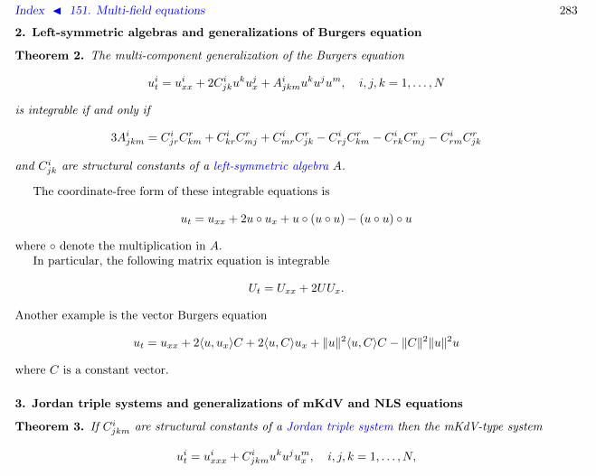
Index J 151. Multi-field equations 283

2. Left-symmetric algebras and generalizations of Burgers equation

Theorem 2. The multi-component generalization of the Burgers equation

uit = uixx + 2Cijkukujx +Aijkmu

kujum, i, j, k = 1, . . . , N

is integrable if and only if

3Aijkm = CijrCrkm + CikrC

rmj + CimrC

rjk − CirjCrkm − CirkCrmj − CirmCrjk

and Cijk are structural constants of a left-symmetric algebra A.

The coordinate-free form of these integrable equations is

ut = uxx + 2u ux + u (u u)− (u u) u

where denote the multiplication in A.In particular, the following matrix equation is integrable

Ut = Uxx + 2UUx.

Another example is the vector Burgers equation

ut = uxx + 2〈u, ux〉C + 2〈u,C〉ux + ‖u‖2〈u,C〉C − ‖C‖2‖u‖2u

where C is a constant vector.

3. Jordan triple systems and generalizations of mKdV and NLS equations

Theorem 3. If Cijkm are structural constants of a Jordan triple system then the mKdV-type system

uit = uixxx + Cijkmukujumx , i, j, k = 1, . . . , N,

Index J 151. Multi-field equations 284

the NLS-type system

uit = uixx + Cijkmujvkum, vit = −vixx − Cijkmvjukvm, i, j, k = 1, . . . , N

and the DNLS-type system

uit = uixx + Cijkm(ujvkum)x, vit = −vixx − Cijkm(vjukvm)x, i, j, k = 1, . . . , N

possess higher symmetries.

The algebraic forms of these system are, respectively,

ut = uxxx + u, u, ux,ut = uxx + 2u, v, u, vt = −vxx − 2v, u, v,ut = uxx + 2v, u, vx, vt = −vxx − 2u, v, ux.

In particular, the simple Jordan triple systems (92.3), (92.4) and (92.5) correspond to the followingintegrable vector and matrix generalizations of KdV equation

ut = uxxx + ‖u‖2ux, u ∈ RN

ut = uxxx + ‖u‖2ux + 〈u, ux〉u, u ∈ RN ,Ut = Uxxx + U2Ux + UxU

2, U ∈ MatN .

The vector generalizations of NLS are of the form

ut = uxx + 2〈u, v〉u, vt = −vxx − 2〈v, u〉v

and

ut = uxx + 4〈u, v〉u− 2‖u‖2v, vt = −vxx − 4〈v, u〉v + 2‖v‖2u.

Index J 151. Multi-field equations 285

4. Deformations of Jordan triple systems

Consider now non-polynomial integrable equations such as

uxy =uxuyu

,

ut = uxxx −3

2

u2xx

ux,

ut = uxx −2

u+ vu2x, vt = −vxx +

2

u+ vv2x.

How to generalize these equations to the multi-component case? What is u−1?

In the scalar case we can define x−1 as a solution of ODE y′ = −y2.

Let X,Y, Z be a Jordan triple system, φ(u) be a solution of the following overdetermined consistentsystem

∂φ

∂uk= −φ, ek, φ, k = 1, . . . , N, (2)

where e1, . . . , eN is a basis of the Jordan triple system and u = uiei.

In the matrix case one of the solutions is

φ(U) = U−1.

For the vector Jordan triple system (92.4)

φ(u) =u

‖u‖2.

An analog of u−1 is well-known in the theory of the Jordan triple systems. Let us define a linear operatorPX by the formula PX(Y ) = X,Y,X. Then, by definition, u−1 = P−1

u (u).

Introduce the notation

αu(X,Y ) = X,φ(u), Y , σu(X,Y, Z) = X, φ(u), Y, φ(u), Z.

Index J 151. Multi-field equations 286

Class 1. For any Jordan triple system the Jordan chiral field equation

uxy = αu(ux, uy)

is integrable. The terminology originates from the matrix case which corresponds to the equation of theprincipal chiral field

uxy =1

2(uxu

−1uy + uyu−1ux), u ∈ GLN .

Class 2. The following equation

ut = uxxx − 3αu(ux, uxx) +3

2σu(ux, ux, ux).

is integrable. Matrix and vector equations have the following form:

ut = uxxx −3

2uxu

−1uxx −3

2uxxu

−1ux +3

2uxu

−1uxu−1ux,

ut = uxxx −3〈u, ux〉‖u‖2

uxx − 3〈u, uxx〉‖u‖2

ux + 3〈ux, uxx〉‖u‖2

u− 3

2

‖ux‖2

‖u‖2ux + 6

〈u, ux〉2

‖u‖4ux − 3

〈u, ux〉‖ux‖2

‖u‖4u,

ut = uxxx −3

2

〈C, ux〉〈C, u〉

uxx −3

2

〈C, uxx〉〈C, u〉

ux +3

2

〈C, ux〉2

〈C, u〉2ux.

Class 3. The following integrable equations

vt = vxxx −3

2αvx(vxx, vxx)

are related to ones of Class 2 by the potentiation u = vx. The matrix equation is

Ut = Uxxx −3

2UxxU

−1x Uxx.

Index J 151. Multi-field equations 287

Vector equations are of the form:

ut = uxxx − 3〈ux, uxx〉‖ux‖2

uxx +3

2

‖uxx‖2

‖ux‖2ux

and

ut = uxxx −3

2

〈C, uxx〉〈C, ux〉

uxx.

Class 4. The scalar representative of this class is the Heisenberg model

ut = uxx −2

u+ vu2x, vt = −vxx +

2

u+ vv2x.

The following coupled equation

ut = uxx − 2αu+v(ux, ux), vt = −vxx + 2αu+v(vx, vx)

is integrable. This equation has a higher symmetry of the form

ut = uxxx − 6αu+v(ux, uxx) + 6σu+v(ux, ux, ux), vt = vxxx − 6αu+v(vx, vxx) + 6σu+v(vx, vx, vx).

The matrix equation from this class is of the form

ut = uxx − 2ux(u+ v)−1ux, vt = −vxx + 2vx(u+ v)−1vx

and one of the two vector equations is

ut = uxx − 4〈ux, u+ v〉‖u+ v‖2

ux + 2‖ux‖2

‖u+ v‖2(u+ v), vt = −vxx + 4

〈vx, u+ v〉‖u+ v‖2

vx − 2‖vx‖2

‖u+ v‖2(u+ v).

Index J 151. Multi-field equations 288

5. Integrable equations of geometric type

Consider multi-component systems of the form

uit = uixxx + aijk(~u)ujxukxx + bijks(~u)ujxu

kxu

sx.

This class is invariant under point transformations ~v = ~Ψ(~u). Under these transformations, the functionsaijk(~u) are transformed as components of an affine connection Γ.

It is convenient to rewrite the system as

uit = uixxx + 3αijkujxu

kxx +

(∂αikm∂uj

+ 2αijrαrkm − αirjαrkm + βijkm

)ujxu

kxu

mx ,

where βijkm = βikjm = βimkj , i.e.

β(X,Y, Z) = β(Y,X,Z) = β(X,Z, Y )

for any vectors X,Y, Z. The set of functions βijkm are transformed just as components of a tensor.Let R and T be the curvature and torsion tensors of Γ.In order to formulate classification results, we introduce the following tensor:

σ(X,Y, Z) = β(X,Y, Z)− 1

3δ(X,Y, Z) +

1

3δ(Z,X, Y ),

whereδ(X,Y, Z) = T (X,T (Y,Z)) +R(X,Y, Z)−∇X(T (Y, Z)).

It follows from the Bianchi identity that

σ(X,Y, Z) = σ(Z, Y,X).

Theorem 4. The system is integrable if and only if

∇X [R(Y,Z, V )] = R(Y,X, T (Z, V )),

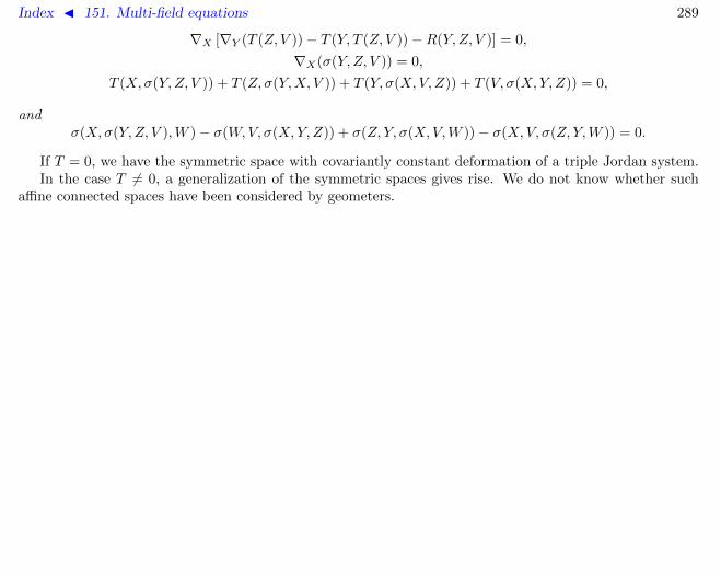
Index J 151. Multi-field equations 289

∇X [∇Y (T (Z, V ))− T (Y, T (Z, V ))−R(Y,Z, V )] = 0,

∇X(σ(Y, Z, V )) = 0,

T (X,σ(Y,Z, V )) + T (Z, σ(Y,X, V )) + T (Y, σ(X,V, Z)) + T (V, σ(X,Y, Z)) = 0,

andσ(X,σ(Y,Z, V ),W )− σ(W,V, σ(X,Y, Z)) + σ(Z, Y, σ(X,V,W ))− σ(X,V, σ(Z, Y,W )) = 0.

If T = 0, we have the symmetric space with covariantly constant deformation of a triple Jordan system.In the case T 6= 0, a generalization of the symmetric spaces gives rise. We do not know whether such

affine connected spaces have been considered by geometers.

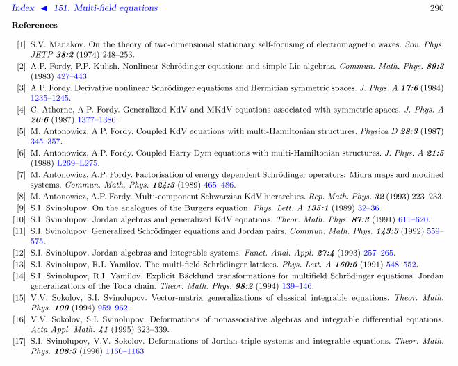
Index J 151. Multi-field equations 290

References

[1] S.V. Manakov. On the theory of two-dimensional stationary self-focusing of electromagnetic waves. Sov. Phys.JETP 38:2 (1974) 248–253.

[2] A.P. Fordy, P.P. Kulish. Nonlinear Schrodinger equations and simple Lie algebras. Commun. Math. Phys. 89:3(1983) 427–443.

[3] A.P. Fordy. Derivative nonlinear Schrodinger equations and Hermitian symmetric spaces. J. Phys. A 17:6 (1984)1235–1245.

[4] C. Athorne, A.P. Fordy. Generalized KdV and MKdV equations associated with symmetric spaces. J. Phys. A20:6 (1987) 1377–1386.

[5] M. Antonowicz, A.P. Fordy. Coupled KdV equations with multi-Hamiltonian structures. Physica D 28:3 (1987)345–357.

[6] M. Antonowicz, A.P. Fordy. Coupled Harry Dym equations with multi-Hamiltonian structures. J. Phys. A 21:5(1988) L269–L275.

[7] M. Antonowicz, A.P. Fordy. Factorisation of energy dependent Schrodinger operators: Miura maps and modifiedsystems. Commun. Math. Phys. 124:3 (1989) 465–486.

[8] M. Antonowicz, A.P. Fordy. Multi-component Schwarzian KdV hierarchies. Rep. Math. Phys. 32 (1993) 223–233.

[9] S.I. Svinolupov. On the analogues of the Burgers equation. Phys. Lett. A 135:1 (1989) 32–36.

[10] S.I. Svinolupov. Jordan algebras and generalized KdV equations. Theor. Math. Phys. 87:3 (1991) 611–620.

[11] S.I. Svinolupov. Generalized Schrodinger equations and Jordan pairs. Commun. Math. Phys. 143:3 (1992) 559–575.

[12] S.I. Svinolupov. Jordan algebras and integrable systems. Funct. Anal. Appl. 27:4 (1993) 257–265.

[13] S.I. Svinolupov, R.I. Yamilov. The multi-field Schrodinger lattices. Phys. Lett. A 160:6 (1991) 548–552.

[14] S.I. Svinolupov, R.I. Yamilov. Explicit Backlund transformations for multifield Schrodinger equations. Jordangeneralizations of the Toda chain. Theor. Math. Phys. 98:2 (1994) 139–146.

[15] V.V. Sokolov, S.I. Svinolupov. Vector-matrix generalizations of classical integrable equations. Theor. Math.Phys. 100 (1994) 959–962.

[16] V.V. Sokolov, S.I. Svinolupov. Deformations of nonassociative algebras and integrable differential equations.Acta Appl. Math. 41 (1995) 323–339.

[17] S.I. Svinolupov, V.V. Sokolov. Deformations of Jordan triple systems and integrable equations. Theor. Math.Phys. 108:3 (1996) 1160–1163

Index J 151. Multi-field equations 291

[18] I.T. Habibullin, V.V. Sokolov, R.I. Yamilov. Multi-component integrable systems and nonassociative structures.pp. 139–168 in: Nonlinear Physics: Theory and Experiment, Lecce’95 (eds E. Alfinito, M. Boiti, L. Martina, F.Pempinelli) Singapore: World Scientific, 1996.

[19] B.A. Kupershmidt. KP or mKP. Noncommutative mathematics of Lagrangian, Hamiltonian, and integrablesystems. Math. Surveys and Monographs 78, Providence, RI: AMS, 2000.

Index J 152. Multi-Hamiltonian structure 292

152 Multi-Hamiltonian structure

Author: A.Ya. Maltsev, 2.10.2009

The Poisson brackets ·, ·1, ·, ·2 form the consistent pair [1] if the linear pencil ·, ·1 + α·, ·2 defines aPoisson bracket as well. Obviously, only the Jacobi identity needs the check, moreover, it is easy to showthat if it holds at some particular value α 6= 0 then it holds for any α.

The equation (ODE, D∆E or PDE) possesses the bi-Hamiltonian structure if it can be represented inthe form

ut = u,H11 = u,H22with the consistent pair of brackets. Analogously, the tri-Hamiltonian structure is defined by equations

ut = u,H11 = u,H22 = u,H33

where the brackets form the consistent triple, that is the operation ·, ·1 + α·, ·2 + β·, ·3 is a Poissonbracket for all α, β.

Consider in more details the finite-dimensional situation corresponding to the pair of Poisson bracketson Mn defined by the structure matrices J ij1 (x) and J ij2 (x). By the definition, they are compatible if thetensor

J ij1 + λJ ij2

defines a Poisson bracket on Mn for every value of λ. It is not difficult to check that this amounts to theJacobi identities for both J ij1 and J ij2 plus the condition that the Schouten bracket

J1, J2ijkSch = J iq1∂Jjk2

∂xq+ Jjq1

∂Jki2

∂xq+ Jkq1

∂J ij2∂xq

+ J iq2∂Jjk1

∂xq+ Jjq2

∂Jki1

∂xq+ Jkq2

∂J ij1∂xq

vanishes identically on Mn.If both J ij1 and J ij2 are non-degenerate then the recursion operator

Rij = J iq2 ||J−11 ||qj

can be defined and has non-zero eigenvalues.

Index J 152. Multi-Hamiltonian structure 293

All the eigenvalues of Rij are double-degenerated and generically Rij has m = n/2 distinct eigenvalues

(λ1, . . . , λm). The eigenvalues of Rij as the functions of x give the set of Hamiltonian functions whichcommute with each other in both the Poisson structures J1 and J2. In the case when the m eigenvalues ofRij are functionally independent and have compact common level surfaces every eigenvalue of Rij generates anintegrable system in both of the two compatible Poisson structures. We get then the infinite set of integrablesystems generated by Hamiltonian functions depending on eigenvalues of Rij only according to the first orthe second Poisson structure J1 or J2. Both these sets of integrable systems coincide with each other andall the systems commute with each other as the dynamical systems.

The recursion operator Rij gives a possibility to define the higher Poisson brackets J ijN , N ≥ 1 accordingto the formula

J ijN =(RN−1

)iqJqj1 .

All brackets J ijN are compatible with each other and give the Poisson structures for the integrable systemsconsidered above. (In fact the same is true also for N ≤ 0). This construction permits to introducethe Hamiltonian hierarchy of integrable systems (see integrable hierarchy) for every Hamiltonian functionH1(λ1, . . . , λm) according to the formula

dxi

dtN= J ijN

∂H1

∂xj.

All the systems from the hierarchy commute with each other and are Hamiltonian with respect to everybracket from the constructed set. It is possible to introduce also the hierarchy of Hamiltonian functions HN

such that

dxi

dtN= J ij1

∂HN

∂xj.

All functions HN depend on eigenvalues (λ1, . . . , λm) only and give the conservation laws for the dynamicalsystems (only m of them are functionally independent).

The construction described above plays the basic role in the case of compatible brackets of constantrank. In this case the integrable systems arise in many examples as the hierarchies generated by the Casimirfunctions of the first bracket considered as the Hamiltonian functions in the second Poisson structure. All

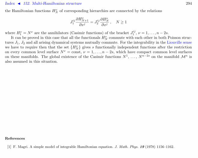
Index J 152. Multi-Hamiltonian structure 294

the Hamiltonian functions HνN of corresponding hierarchies are connected by the relations

J ij1∂Hν

N+1

∂xj= J ij2

∂HνN

∂xj, N ≥ 1

where Hν1 = Nν are the annihilators (Casimir functions) of the bracket J ij1 , ν = 1, . . . , n− 2s.

It can be proved in this case that all the functionals HνN commute with each other in both Poisson struc-

tures J1, J2 and all arising dynamical systems mutually commute. For the integrability in the Liouville sensewe have to require then that the set Hν

N gives s functionally independent functions after the restrictionon every common level surface Nν = const, ν = 1, . . . , n − 2s, which have compact common level surfaceson these manifolds. The global existence of the Casimir functions N1, . . . , Nn−2s on the manifold Mn isalso assumed in this situation.

References

[1] F. Magri. A simple model of integrable Hamiltonian equation. J. Math. Phys. 19 (1978) 1156–1162.

Index J 153. Neumann system D 295

153 Neumann system

u = −Ju+ (〈u, Ju〉 − 〈u, u〉)u, u ∈ Rd, |u| = 1, J = diag(J1, . . . , Jd)

ã This system, introduced in [1], describes the motion of a particle on the sphere in the quadratic potential12 〈u, Ju〉. It describes also a certain class of exact solutions of Landau–Lifshitz equation [2].

ã Several discrete-time integrable systems on the sphere are known, of the general form

un+1 = F (un, un−1;K), un ∈ Rd, |un| = 1, K = diag(K1, . . . ,Kd),

which have the Neumann system as the continuous limit [3]. Although these discretizations possess thedifferent sets of the invariants which are not equivalent even at d = 3, the corresponding dynamics is verysimilar. The plots below show the evolution of the same initial data (at the same choice of the parametermatrix K).

Veselov discretization Ragnisco discretization Adler discretization

-1

-0.5

0

0.5

1

-1

-0.5

0

0.5

1

-1

-0.5

0

0.5

1

-1

-0.5

0

0.5

-1

-0.5

0

0.5

-1

-0.5

0

0.5

1

-1

-0.5

0

0.5

1

-1

-0.5

0

0.5

1

-1

-0.5

0

0.5

-1

-0.5

0

0.5

-1

-0.5

0

0.5

1

-1

-0.5

0

0.5

1

-1

-0.5

0

0.5

1

-1

-0.5

0

0.5

-1

-0.5

0

0.5

Index J 153. Neumann system D 296

References

[1] C. Neuman. De problemate quodam mechanica, quod ad primam integralium ultraellipticorum classem revo-catur. J. Reine Angew. Math. 56 (1859) 46–69.

[2] A.P. Veselov. Landau–Lifshitz equation and integrable systems of classical mechanics. Dokl. Akad. Nauk SSSR270:5 (1983) 1094–1096.

[3] Yu.B. Suris. The problem of integrable discretization: Hamiltonian approach. Basel: Birkhauser, 2003.

Index J 154. Neumann system, Adler discretization ∆ 297

154 Neumann system, Adler discretization

un+1 + un1 + 〈un, un+1〉

+un + un−1

1 + 〈un, un−1〉=

2Kun〈un,Kun〉

, un ∈ Rd, |un| = 1, K = diag(K1, . . . ,Kd)

ã Continuous limit: un = u(2εn), K = I − ε2J .

ã The invariants:

I1 =〈Kun, un+1〉

1 + 〈un, un+1〉, I2 =

〈K−1(un + un+1), (un + un+1)〉(1 + 〈un, un+1〉)2

, . . .

References

[1] V.E. Adler. Discretizations of the Landau–Lifshitz equation. Theor. Math. Phys. 124:1 (2000) 897–908.

Index J 155. Neumann system, Ragnisco discretization ∆ 298

155 Neumann system, Ragnisco discretization

un+1

〈un, un+1〉−2un+

un−1

〈un, un−1〉= −K−2un+〈un,K−2un〉un, un ∈ Rd, |un| = 1, K = diag(K1, . . . ,Kd)

Continuous limit: un = u(εn), K−2 = ε2J .

References

[1] O. Ragnisco. A discrete Neumann system. Phys. Lett. A 167:2 (1992) 165–171.

Index J 156. Neumann system, Veselov discretization ∆ 299

156 Neumann system, Veselov discretization

un+1 + un−1 =2〈Kun, un−1〉〈K2un, un〉

Kun, un ∈ Rd, |un| = 1, K = diag(K1, . . . ,Kd)

Alias: stationary Heisenberg spin chain

ã Continuous limit: un = u(εn), K−2 = I + ε2J .

ã The invariants:

I1 = 〈Kun, un+1〉, I2 = 〈K−2un, un〉+ 〈K−2un+1, un+1〉 − 〈K−1un, un+1〉2, . . .

References

[1] A.P. Veselov. Integration of the stationary problem for classical spin lattice. Theor. Math. Phys. 71:1 (1987)446–450

[2] Ya.I. Granovsky, A.C. Zhedanov. Domain-type solutions in anisotropic magnetic chains. Theor. Math. Phys.71:1 (1987) 438–446

Index J 157. Noether theorem 300

157 Noether theorem

Author: A.B. Shabat, 27.02.2007

By a conservation law for a differential system

ωa(x, u, ui, . . . ) = 0, i = 1, . . . ,m+ 1, a = 1, . . . , n,

uai = ∂ua/∂xi, xi = (x1, x2, . . . , xm, t)

is meant a continuity equation∑DiKi ≡ 0, Ki = Ki(x, u, uj , . . . ), i, j = 1, . . . ,m+ 1,

which is satisfied for any solutions of the original system. Each conservation law is defined up to an equiv-alence transformation Ki → Ki + Pi,

∑DiPi ≡ 0. Two conservation laws belong to the same equivalence

class if they differ by a trivial conservation law. For trivial conservation laws the components of the vectorKi vanish on the solutions: Ki = 0, (i, j = 1, . . . ,m+ 1), or the continuity equation is satisfied in the wholespace:

∑DiKi ≡ 0; first and second types of triviality, respectively.

We consider functions u = u(x) defined on a region D of (m+ 1)-dimensional space-time. Let

S =

∫D

L(xi, ua, uai , . . . )dm+1x

be the action functional, where L is the Lagrangian density. Then the equations of motion are

Ea(L) = ωa(x, u, ui, uij . . . ) = 0, i, j = 1, . . . ,m+ 1, a = 1, . . . , n

where E is the Euler–Lagrange operator

Ea =∂

∂ua−∑i

Di∂

∂uai+∑i≤j

DiDj∂

∂uaij+ . . . .

Index J 157. Noether theorem 301

Consider an evolutionary vector field

Xα = αa∂

∂ua+∑i

(Diαa)

∂

∂uai+∑i≤j

(DiDjαa)

∂

∂uaij+ . . . αa = αa(x, u, ui, . . . ). (1)

Variation of the functional S under this infinitesimal transformation with operator Xα is

δS =

∫D

XαLdm+1x.

Xα is a variational (Noether) symmetry if

XαL = DiMi, Mi = Mi(x, u, uj , . . . ), i = 1, . . . , m+ 1, (2)

The Noether identity

Xα = αaEa +DiRαi, Rαi = αa∂

∂uai+

∑k≥i

(Dkαa)− αa

∑k≤i

Dk

∂

∂uaik+ . . .

in application to (2) we will obtainDi(Mi −RαiL) = αaωa ≡ 0 (3)

on the solution manifold (ω = 0, Diω = 0, . . . ).Thus, any 1-parameter variational symmetry transformation Xα (1) leads to a conservation law (3).

Index J 158. Nonlinear Klein-Gordon equation hDD 302

158 Nonlinear Klein-Gordon equation

utt − ux1x1 − · · · − uxdxd= F (u)

The equation is not integrable at d > 1 for any nonlinear F . At d = 1 the integrable nonlinear cases areexhausted, up to the point transforms, by three equations [2]:

ã uxy = eu the Liouville equation;

ã uxy = sinu the sine-Gordon equation;

ã uxy = e2u − e−u the Tzitzeica equation.

References

[1] G.B. Whitham. Linear and nonlinear waves, N.Y.: Wiley, 1974.

[2] A.V. Zhiber, A.B. Shabat. Nonlinear Klein–Gordon equations with nontrivial group. Dokl. Akad. Nauk SSSR247:5 (1979) 1103–1107.

Index J 159. Nonlinear Schrodinger equation eDD 303

159 Nonlinear Schrodinger equation

ut = uxx + 2u2v, −vt = vxx + 2v2u. (1)

Aliases: Zakharov–Shabat, Ablowitz–Kaup–Newell–Segur system

ã Third order symmetry:ut3 = uxxx + 6uvux, vt3 = vxxx + 6uvvx. (2)

ã Backlund–Schlesinger transformation:

u1 = uxx − u2x/u+ u2v, v1 = 1/u. (3)

The iterations of this mapping are governed, under the change u = eq, v = e−q−1 , by the Toda lattice

qxx = eq1−q − eq−q−1 . (4)

ã Chain of Backlund–Darboux transformations:

un,x = un+1 + αnun + u2nvn+1, −vn,x = vn−1 + αn−1vn + un−1v

2n (5)

vm, un = δm,n+1, H =∑(

unvn + αnunvn+1 +1

2u2nv

2n+1

)where αn are arbitrary parameters. A generic BT for the NLS equation is decomposed as a sequence ofelementary transformations of the form (3), (5) and their inverses.

ã Permutability of the transformations (3) and (5) gives rise to 5-point equations of discrete Toda type

eq1,−i−q − eq−q−1,i + eqi−q − eq−q−i + α(i) − α(i)−i = 0. (6)

ã Nonlinear superposition principle:

un = un −(αn+1 − αn)un−1

1− un−1vn+1, vn = vn +

(αn+1 − αn)vn+1

1− un−1vn+1(7)

Index J 159. Nonlinear Schrodinger equation eDD 304

ã Zero curvature representation Ut = Vx + [V,U ], Wx = U1W −WU :

U =

(λ −vu −λ

), V = −2λU +

(−uv vxux uv

),

Wn =

(1 −vn+1

un −2λ− unvn+1 − βn

)ã Recursion operator:(

u

v

)tn

= Rn(u

v

), R =

(Dx + 2uD−1

x v 2uD−1x u

−2vD−1x v −Dx − 2vD−1

x u

)

References

[1] V.E. Zakharov. Stability of periodic waves of finite amplitude on the surface of a deep fluid. J. Appl. Mechanicsand Technical Physics 9:2 (1968) 190–194.

Index J 160. Nonlinear Schrodinger equation, matrix eDD 305

160 Nonlinear Schrodinger equation, matrix

ut = uxx + 2uvu, −vt = vxx + 2vuv, u ∈ MatM,N (C), v ∈ MatN,M (C)

ã Backlund transformation:

un,x = un+1 + βnun + unvn+1un, −vn,x = vn−1 + βn−1vn + vnun−1vn

Third order symmetry:

ut = uxxx + 3uxvu+ 3uvux, vt = vxxx + 3vxuv + 3vuvx.

ã Zero curvature representation

U =

(−λMIN −v

u λNIM

), V = λ(M +N)U +

(−vu vxux uv

)Wn =

(IN −vn+1

un λ(M +N)IM − βnIM − unvn+1

).

The M ×M matricesU = −2uv, W = 2uvx − 2uxv

satisfy the matrix KP equation

4Ut3 = Uxxx − 3(UxU + UUx −Wt + [W,U ]), Wx = Ut,

and the matrices

Fn = −unvn+1 − βnIM , Pn = unvn+1,x − un,xvn+1 + unvn+1unvn+1 − β2nIM

satisfy the two-dimensional matrix dressing chain

Fn+1,x + Fn,x = F 2n+1 − F 2

n + Pn+1 − Pn, Pn,x = Fn,t + [Pn, Fn].

Index J 160. Nonlinear Schrodinger equation, matrix eDD 306

References

[1] V.E. Zakharov. The inverse scattering method. p. 243 in: Solitons. (R.K. Bullough, P.J. Caudrey eds) Topicsin current physics 17, Springer-Verlag, 1980.

[2] V.A. Marchenko. Nonlinear equations and operator algebras. Boston: Reidel, 1988.

[3] A.P. Fordy, P.P. Kulish. Nonlinear Schrodinger equations and simple Lie algebras. Commun. Math. Phys. 89:3(1983) 427–443.

[4] B.G. Konopelchenko. Nonlinear transformations and integrable evolution equations. Fortschr. Phys. 31 (1983)253–296.

Index J 161. Nonlinear Schrodinger equation, multidimensional eDN 307

161 Nonlinear Schrodinger equation, multidimensional

iψt = ∆ψ + |ψ|2σψ, ∆ = ∇2 = ∂2x1

+ · · ·+ ∂2xn

(1)

ã This equation arises in a number of physical problems, such as plasma physics and nonlinear optics [1].Not integrable. Some particular solutions describing the weak collapse and governed by ODE of Painlevetype were studied in [2, 3, 4].

The conserved densities:

|ψ|2, i

2(ψ∇ψ∗ − ψ∗∇ψ),

1

2|∇ψ|2 − 1

σ + 1|ψ|2σ+2.

References

[1] V.E. Zakharov, V.S. Synakh. On the character of selffocusing singularity. Sov. Phys. JETP 42 (1976) 464.

[2] Yu.N. Ovchinnikov. Weak collapse in the nonlinear Schrodinger equation. JETP Lett. 69:5 (1999) 418–422.

[3] Yu.N. Ovchinnikov, V.L. Vereshchagin. Asymptotic behavior of weakly collapsing solutions of the nonlinearSchrodinger equation. JETP Lett. 74:2 (2001) 72–76.

[4] C. Budd, V. Dorodnitsyn. Symmetry-adapted moving mesh schemes for the nonlinear Schrodinger equation. J.Phys. A 34:48 (2001) 10387–10400.

Index J 162. Nonlinear Schrodinger equation, Jordan eDD 308

162 Nonlinear Schrodinger equation, Jordan

ut = uxx + 2uvu, −vt = vxx + 2vuv, u ∈ V +, v ∈ V −

where V = (V +, V −) is a Jordan pair.

This is the most general multifield version of NLS. The particular cases are:

ã the matrix NLS system;ã the Manakov vectorial NLS system;ã the Kulish–Sklyanin vectorial NLS system.

ã Third order symmetry:

ut = uxxx + 6uvux, vt = vxxx + 6vuvx.

ã Backlund transformation::

uj,x = uj+1 + βjuj + ujvj+1uj, −vj,x = vj−1 + βj−1vj + vjuj−1vj

ã Zero curvature representation Ut = Vx + [V,U ] is given in terms of the structure Lie algebra of Jordanpair:

U = u− 2v + λσ, V = ux + 2vx + 2L(u, v) + λU

ã The differential substitution v = −wx − wuw (equivalent to the shift vj+1 → vj in the chain of BT)brings to the modified Jordan NLS

ut = uxx − 2uwxu − 2uwuwu, −wt = wxx + 2wuxw − 2wuwuw

which is the symmetry of the PLR-type hyperbolic system

uxy = 2uwuy − u, wxy = −2wuwy − w.

Index J 162. Nonlinear Schrodinger equation, Jordan eDD 309

References

[1] S.I. Svinolupov. Generalized Schrodinger equations and Jordan pairs. Commun. Math. Phys. 143:3 (1992) 559–575.

Index J 163. Nonlinear Schrodinger equation, vectorial eDD 310

163 Nonlinear Schrodinger equation, vectorial

Author: V.E. Adler, 2007.02.05

ut = uxx + 4〈u, v〉u− 2〈u, u〉v, −vt = vxx + 4〈u, v〉v − 2〈v, v〉u, u, v ∈ Cm. (1)

Alias: Kulish–Sklyanin system

ã Introduced in [1].

ã Third order symmetry:

ut = uxxx + 6〈u, v〉ux + 6〈ux, v〉u− 6〈u, ux〉v,vt = vxxx + 6〈u, v〉vx + 6〈u, vx〉v − 6〈v, vx〉u. (2)

ã Backlund–Schlesinger transformation [2]:

u1 = uxx − 2〈u, ux〉〈u, u〉

ux +〈ux, ux〉〈u, u〉

u+ 2〈u, v〉u− 〈u, u〉v, v1 =1

〈u, u〉u, (3)

ã Backlund–Darboux transformation:

ux = ui + α(i)u+ 2〈u, vi〉u− 〈u, u〉vi, −vi,x = v + α(i)vi + 2〈u, vi〉vi − 〈vi, vi〉u. (4)

ã Nonlinear superposition principle [3]:

uj = ui +(α(i) − α(j))(u− 〈u, u〉vij)

1− 2〈u, vij〉+ 〈u, u〉〈vij , vij〉, vj = vi −

(α(i) − α(j))(vij − 〈vij , vij〉u)

1− 2〈u, vij〉+ 〈u, u〉〈vij , vij〉. (5)

ã Zero curvature representation:

U =

−λ −2vᵀ 0u 0 2v0 −uᵀ λ

, V = λU +

−2vᵀu 2vᵀx 0ux 2uvᵀ − 2vuᵀ −2vx0 −uᵀx 2uᵀv

Index J 163. Nonlinear Schrodinger equation, vectorial eDD 311

W (i) =

1 −2vᵀi −2vᵀi vi

u (λ− α(i))In − 2uvᵀi 2(λ− α(i) − uvᵀi )vi

− 12u

ᵀu uᵀ(uvᵀi − λ+ α(i)) (λ− α(i))2 − 2(λ− α(i))uᵀvi + uᵀuvᵀi vi

ã Kulish–Sklyanin hierarchy is a squared eigenfunction constraint for the Hirota–Ohta hierarchy:

Statement 1. Equations (1)–(5) are consistent and, in virtue of these equations, the quantities

U = −〈u, u〉, V = −〈v, v〉, W = 4〈u, v〉, Q = 4〈ux, v〉 − 4〈u, vx〉,

W (i) = α(i) + 2〈u, vi〉, W (ij) =α(i) − α(j)

1− 2〈u, vij〉+ 〈u, u〉〈vij , vij〉

satisfy the equations of the Hirota–Ohta hierarchy.

References

[1] P.P. Kulish, E.K. Sklyanin. O(N)-invariant nonlinear Schrodinger equation — a new completely integrablesystem. Phys. Lett. A 84:7 (1981) 349–352.

[2] S.I. Svinolupov, R.I. Yamilov. Explicit Backlund transformations for multifield Schrodinger equations. Jordangeneralizations of the Toda chain. Theor. Math. Phys. 98:2 (1994) 139–146.

[3] V.E. Adler. Nonlinear superposition formula for Jordan NLS equations. Phys. Lett. A 190 (1994) 53–58.

Index J 164. Nonlinear Schrodinger equation, derivative eDD 312

164 Nonlinear Schrodinger equation, derivative

ut = uxx + 2(u2v)x, vt = −vxx + 2(uv2)x

Alias: Kaup–Newell system, DNLS-I; Namesakes: Chen–Lee–Liu system (DNLS-II), Gerdjikov–Ivanov equa-tion (DNLS-III)

ã Master-symmetry:

uτ = (xux + 2xu2v + cu)x, vτ = (−xvx + 2xuv2 + (c− 1)v)x

ã Higher symmetry:

ut3 = (uxx + 6uuxv + 6u3v2)x, vt3 = (vxx − 6uvvx + 6u2v3)x

ã Backlund transformation:

un,x = u2n(un+1 − un−1), un,t = u2

n(u2n+1(un+2 + un)− u2

n−1(un − un−2)), u = un, v = un−1.

ã Zero curvature representation

U = 2λ

(λ u−v −λ

), V = (4λ2 + 2uv)U + 2λ

(0 uxvx 0

), L =

(2λ/u 1−1 0

).

References

[1] D.J. Kaup, A.C. Newell. An exact solution for a derivative nonlinear Schrodinger equation. J. Math. Phys. 19:4(1978) 798–801.

Index J 165. Nonlinear Schrodinger equation, Jordan derivative eDD 313

165 Nonlinear Schrodinger equation, Jordan derivative

ut = uxx + 2uvux, vt = −vxx + 2vuvx, u ∈ V +, v ∈ V −

where V = (V +, V −) is a Jordan pair.This is the most general multifield version of the DNLS-I equation.Third order symmetry:

ut3 = (uxx + 6uvux+ 6uvuvu)x, vt3 = (vxx − 6vuvx+ 6vuvuv)x.

References

[1] A.P. Fordy. Derivative nonlinear Schrodinger equations and Hermitian symmetric spaces. J. Phys. A 17:6 (1984)1235–1245.

[2] V.E. Adler, S.I. Svinolupov, R.I. Yamilov. Multi-component Volterra and Toda type integrable equations. Phys.Lett. A 254 (1999) 24–36.

Index J 166. Nonlinear Schrodinger equation, matrix derivative eDD 314

166 Nonlinear Schrodinger equation, matrix derivative

ut = uxx + 2(uvᵀu)x, vt = −vxx + 2(vuᵀv)x, u, v ∈ Matm,n(C)

This and some others matrix versions of DNLS-type equations were studied in [1, 2, 3].

References

[1] P.J. Olver, V.V. Sokolov. Integrable evolution equations on associative algebras. Commun. Math. Phys. 193:2(1998) 245–268.

[2] P.J. Olver, V.V. Sokolov. Non-abelian integrable systems of the derivative nonlinear Schrodinger type. InverseProblems 14:6 (1998) L5–L8.

[3] T. Tsuchida, M. Wadati. Complete integrability of derivative nonlinear Schrodinger-type equations. InverseProblems 15 (1999) 1363–1373.

Index J 167. Nonlinear Schrodinger equation, vectorial derivative eDD 315

167 Nonlinear Schrodinger equation, vectorial derivative

ut = uxx + 2(〈u, v〉u)x, vt = −vxx + 2(〈u, v〉v)x, u, v ∈ Cn

References

[1] H.C. Morris, R.K. Dodd. Physica scripta 20 (1979) 505.

Index J 168. Nonlinear Schrodinger type systems, classification eDD 316

168 Nonlinear Schrodinger type systems, classification

Author: V.E. Adler, 09.01.2009

1. Introduction

2. Extension of the module of the point transformations

3. The list of integrable systems

4. Substitutions

5. Necessary integrability conditions

1. Introduction

The classification problem of NLS type integrable systems

wt = A(w)w2 + F (w,w1), w = (u, v)ᵀ, F = (f, g)ᵀ, detA 6= 0 (1)

within the symmetry approach was considered in the papers [1] where the necessary conditions were obtainedfor the existence of the higher order conservations laws. These conditions separate out the nonintegrablecases as well as the linearizable systems of Burgers type which possess higher symmetries, but do not possessthe higher conservations laws. In particular, it turned out that all systems which satisfy these conditionscan be brought to the form

ut = u2 + f(u, v, u1, v1), −vt = u2 + g(u, v, u1, v1) (2)

by use of a differential substitution. Further classification was done modulo point changes plus so-calledsymmetric transformations. In the final form this problem was solved in the paper [2], see also [3, 4].Several systems appeared to be new and their integrability was justified either by establishing a differentialsubstitution bringing to a known integrable system either by construction of zero curvature representation.Depending on the order of the auxiliary linear problem, 2 and 3 correspondingly, the list is divided into theNLS-type systems (a–p) and Boussinesq-type systems (q–u6).

Index J 168. Nonlinear Schrodinger type systems, classification eDD 317

2. Extension of the module of the point transformations

The point changes acting on the whole set of the systems (2) are generated by the transformations

(x, t)→ (ax+ bt+ c, a2t+ d), (u, v)→ (φ(u), ψ(v)), (x, t, u, v)→ (−x,−t, v, u). (3)

The numerous subclass consists of the systems which are invariant with respect to some one-parametricgroup of transformations (u, v) → (φ(α, u), ψ(α, v)). One can assume, without loss of generality that thissubgroup consists of the shifts (u, v)→ (u+α, v) or (u, v)→ (u+α, v−α). The corresponding system is ofthe special form

ut = u2 + f(εu+ v, u1, v1), −vt = u2 + g(εu+ v, u1, v1), ε = 0, 1. (4)

Such a system admits the differential substitution of the form u = U(εu + v, u1), v = V (εu + v), whichgenerically leads beyond the class (4). However, there is an important case when a composition of suchsystems preserves the form of the system.

A symmetric system is the system of the form (4) which is invariant with respect to the involution(x, t, u, v)→ (−x,−t, v, u):

ut = u2 + f(u+ v, u1, v1), −vt = u2 + f(u+ v,−v1,−u1). (5)

The following properties are valid.

Theorem 1. Let the system (5) possesses a conservation law with the density ρ = p′(u + v)u1 + q(u + v),p′ 6= 0. Then the symmetric transformation

u+ v = p(u+ v), u1 = p′(u+ v)u1 + q(u+ v) (6)

maps it to another symmetric system. Transformations of this form define the equivalence relation on the setof the systems (5) and preserve the integrability property, that is if the original system possesses the highersymmetries and conservation laws then so its transform does.

The following example demonstrates that the use of symmetric changes allow to reduce essentially thelist of integrable systems.

Index J 168. Nonlinear Schrodinger type systems, classification eDD 318

Example 2. Let us consider the system

ut = u2 + 2auvu1 + bu2v1 +1

2b(a− b)u3v2 + cu2v, −vt = v2 − 2auvv1 − bv2u1 +

1

2b(a− b)u2v3 + cuv2

which includes, for instance, the complexified Gerdjikov–Ivanov system as a particular case. The chageu→ exp(u), v → exp(v) brings it to the form (5) with f = u2

1 + (2au1 + bv1 + c)eu+v + 12b(a− b)e

2u+2v. It isnot difficult to establish, by use of the density ρ = u1 +βeu+v, the symmetric equivalence with the followingsystems:

1) at b = 2a, c = 0 with the linear system (a = b = c = 0);2) at b = 2a, c 6= 0 with NLS (a = b = 0, c = 1);3) at b 6= 2a with DNLS (a = b = 1, c = 0).

3. The list of integrable systems

Theorem 3 ([2]). The systems (2) possessing an infinite set of higher symmetries and conservation laws arereducible to the systems of the following list, up to the transformations (3) and symmetric transformations(6).

Remark. In some instances it is convenient to include the equations which are equivalent modulo theaforementioned transformations. Such systems are denoted by the same letters with primes. The upper- andlower-case marked system are related via potentiation. The other changes are described in the next section.

ut = u2 + u21 + v1, −vt = v2 − 2u1v1; (a)

Kaup–Broer ut = u2 + (u2 + v)x, −vt = v2 − 2(uv)x; (A)

NLS ut = u2 + u2v, −vt = v2 + v2u; (b)

Kaup ut = u2 + (u+ v)u1, −vt = v2 − (u+ v)v1; (c)

ut = u2 + u21v1 − 4v1, −vt = v2 − u1v

21 + 4u1; (d)

ut = u2 + (u2v − 4v)x, −vt = v2 − (uv2 − 4u)x; (D)

Index J 168. Nonlinear Schrodinger type systems, classification eDD 319

ut = u2 −u2

1v1

(u+ v)2− 2u2

1

u+ v, −vt = v2 +

u1v21

(u+ v)2− 2v2

1

u+ v; (d′)

ut = u2 + sech2(u+ v)u2

1v1 − 2 tanh(u+ v)u21,

−vt = v2 − sech2(u+ v)u1v21 − 2 tanh(u+ v)v2

1 ;(d′′)

ut = u2 − 2 tanh(u+ v)(u21 − 4), −vt = v2 − 2 tanh(u+ v)(v2

1 − 4); (e)ut = u2 −

2u21

u+ v− 8(1 + uv)u1 + 4(1− u2)v1

(u+ v)2,

−vt = v2 −2v2

1

u+ v+

8(1 + uv)v1 + 4(1− v2)u1

(u+ v)2;

(f)

ut = u2 + u21v1, −vt = v2 − u1v

21 − u1; (g)

ut = u2 + (u2v)x, −vt = v2 − (uv2 + u)x; (G)

ut = u2 + u21 − 2u1v1, −vt = v2 − v2

1 − 2u1v1; (h)

Levi ut = u2 + (u2 − 2uv)x, −vt = v2 − (v2 − 2uv)x; (H)

Heisenberg ut = u2 −2u2

1

u+ v, −vt = v2 −

2v21

u+ v; (h′)

ut = u2 − 2 tanh(u+ v)u21, −vt = v2 − 2 tanh(u+ v)v2

1 ; (h′′)

ut = u2 + u21v1, −vt = v2 − u1v

21 ; (i)

DNLS ut = u2 + (u2v)x, −vt = v2 − (uv2)x; (I)

ut = u2 + exp(u+ v)u21v1 + u2

1, −vt = v2 − exp(u+ v)u1v21 + v2

1 ; (i′)

ut = u2 −2(u2

1 + 1)

u+ v, −vt = v2 −

2(v21 + 1)

u+ v; (j)

Index J 168. Nonlinear Schrodinger type systems, classification eDD 320ut = u2 −

2u21

u+ v− 4((u− v)u1 + uv1)

(u+ v)2,

−vt = v2 −2v2

1

u+ v+

4((u− v)v1 − u1v)

(u+ v)2;

(k)

ut = u2 +R(y)u2

1v1 +R′(y)u21 −

2

3(R′′(y)− 2c)u1 +

1

3R′′′(y),

−vt = v2 −R(y)u1v21 +R′(y)v2

1 +2

3(R′′(y)− 2c)v1 +

1

3R′′′(y),

(l)

where y = y(u+ v), y′ = R(y) = ay4 + by3 + cy2 + dy + e 6= 0;ut = u2 −

2u21

u+ v− 4(P (u, v)u1 +R(u)v1)

(u+ v)2,

−vt = v2 −2v2

1

u+ v+

4(P (u, v)v1 +R(−v)v1)

(u+ v)2,

(m)

where P (u, v) = 2au2v2 + buv(v − u)− 2cuv + d(u− v) + 2e,

R(y) = ay4 + by3 + cy2 + dy + e;

Landau–Lifshits

ut = u2 −

2(u21 +R(u))

u+ v+R′(u)

2,

−vt = v2 −2(v2

1 +R(−v))

u+ v− R′(−v)

2,

(n)

where R(y) = ay4 + by3 + cy2 + dy + e;ut = u2 + eφ(u2

1 + 1)v1 + φuu21 + 2(y(u+ v) + y(u− v))u1,

−vt = v2 − eφ(v21 + 1)u1 + φvv

21 − 2(y(u+ v) + y(u− v))v1,

(o)

where eφ = y(u+ v)− y(u− v),

(y′)2 = −4y4 + ay3 + by2 + cy + d;

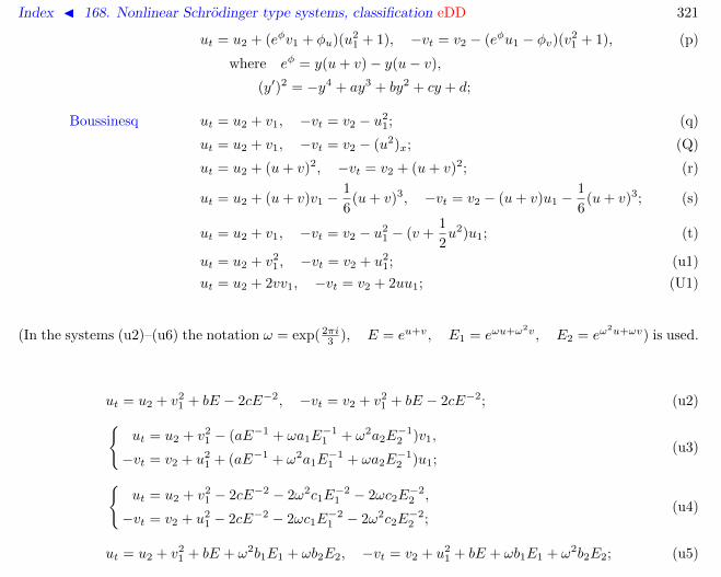
Index J 168. Nonlinear Schrodinger type systems, classification eDD 321

ut = u2 + (eφv1 + φu)(u21 + 1), −vt = v2 − (eφu1 − φv)(v2

1 + 1), (p)

where eφ = y(u+ v)− y(u− v),

(y′)2 = −y4 + ay3 + by2 + cy + d;

Boussinesq ut = u2 + v1, −vt = v2 − u21; (q)

ut = u2 + v1, −vt = v2 − (u2)x; (Q)

ut = u2 + (u+ v)2, −vt = v2 + (u+ v)2; (r)

ut = u2 + (u+ v)v1 −1

6(u+ v)3, −vt = v2 − (u+ v)u1 −

1

6(u+ v)3; (s)

ut = u2 + v1, −vt = v2 − u21 − (v +

1

2u2)u1; (t)

ut = u2 + v21 , −vt = v2 + u2

1; (u1)

ut = u2 + 2vv1, −vt = v2 + 2uu1; (U1)

(In the systems (u2)–(u6) the notation ω = exp( 2πi3 ), E = eu+v, E1 = eωu+ω2v, E2 = eω

2u+ωv) is used.

ut = u2 + v21 + bE − 2cE−2, −vt = v2 + v2

1 + bE − 2cE−2; (u2)ut = u2 + v2

1 − (aE−1 + ωa1E−11 + ω2a2E

−12 )v1,

−vt = v2 + u21 + (aE−1 + ω2a1E

−11 + ωa2E

−12 )u1;

(u3)

ut = u2 + v2

1 − 2cE−2 − 2ω2c1E−21 − 2ωc2E

−22 ,

−vt = v2 + u21 − 2cE−2 − 2ωc1E

−21 − 2ω2c2E

−22 ;

(u4)

ut = u2 + v21 + bE + ω2b1E1 + ωb2E2, −vt = v2 + u2

1 + bE + ωb1E1 + ω2b2E2; (u5)

Index J 168. Nonlinear Schrodinger type systems, classification eDD 322

ut = u2 + v21 − (aE−1 + ωa1E

−11 + ω2a2E

−11 )v1

− 1

6(a1a2E + ω2aa2E1 + ωaa1E2 + a2E−2 + ω2a2

1E−21 + ωa2

2E−22 ),

−vt = v2 + u21 + (aE−1 + ω2a1E

−11 + ωa2E

−12 )u1

− 1

6(a1a2E + ωaa2E1 + ω2aa1E2 + a2E−2 + ωa2

1E−21 + ω2a2

2E−22 );

(u6)

ut = u2 −(u1 + 2v1)u1

2(u+ v)+ a(u+ v), −vt = v2 −

(2u1 + v1)v1

2(u+ v)+ b(u+ v); (v)

ut = u2 + (u2 + v−1)x, −vt = v2 − 2(uv)x − 1. (w)

Index J 168. Nonlinear Schrodinger type systems, classification eDD 323

4. Substitutions

The systems (v), (w) can be brought to the linear and reducible systems, respectively:

(v)→ (ut = u2 + v1 +a− b

2u, −vt = v2 − 2bu1 +

a− b2

v) : u = 2(u+ v)1/2, v = −2v1(u+ v)−1/2,

(w)→ (ut = u2 + 1/v, −vt = v2) : u = u1/u, v = uv.

The other systems are related by the following changes (the symmetric systems are in boxes, the doublearrows denote potentiation u = u1, v = v1, and, as usually, in the substitution marked A → B the tildedvariables correspond to equation B):

(a)

(b)ww c

(A)

d

eww (f)

(D)

g i

j

ww hww (k)

(G)

ww I

(H)

(q)

(r)ww

(Q)

(l) → (m)

s → (t)

u1 ⇒ (U1)

(n) (o) (p)

u2 (u3) (u4) (u5) (u6)

Index J 168. Nonlinear Schrodinger type systems, classification eDD 324

(a)→ (b) u = eu, v = e−uv1

(b)→ (A) u = u1/u, v = uv

(c)→ (A) u = (u+ v)/2, v = −v1

(a)→ (c) u = 2u1 + v, v = −v(d)→ (e) u = atanh(u1/2)− v, v = v

(e)→ (D) u = 2 tanh(u+ v), v = v1

(d′′)→ (f) u = tanh(u+ v), v = − tanh(u+ v)− 2/v1

(g)→ (j) u = 2/u1, v = v

(j)→ (G) u = 2/(u+ v), v = v1

(g)→ (h′′) u = −iu/2, v = iu/2 + atanh(−iv1)

(h′′)→ (G) u = 2iu1, v = i tanh(u+ v)

(h′)→ (I) u = 2/(u+ v), v = v1

(I)→ (H) u = −uv/2, v = −uv/2− v1/v

(i)→ (h′) u = 2/u1 − v1, v = v

(i′)→ (k) u = eu+v, v = −2/v1 − eu+v

(l)→ (m) u = y(u+ v), v = −2/v1 − y(u+ v)

(q)→ (r) u = u1/2 + v/4, v = −v/4(r)→ (Q) u = 2(u+ v), v = −4v1

(s)→ (t) u = −(u+ v), v = 2v1 − (u+ v)2/2

Index J 168. Nonlinear Schrodinger type systems, classification eDD 325

5. Necessary integrability conditions

Statement 4. If the system (1) possesses the conservation law with the density ρ(w,w1, . . . , wn) of nonzeroorder then

trA = 0, tr(A−1Fw1) ∈ ImDx, Dt((detA)−1/4) ∈ ImDx (7)

where Fw1 =(fu1

fv1gu1

gv1

)denotes the Jacobi matrix. Moreover, the density ρ is a polynomial in wn, and its

degree does not exceed 2.

The Statement 4 allows to make the change which simplifies the system to the form (2). The furtherintegrability conditions are computed for the systems which are already in this form. These conditions meanthat the equations

Dt(ρk) = Dx(σk), ωk = Dx(φk), k = 0, 1, 2, . . . (8)

must be solvable with respect to σk, φk, as functions on u, v and their x-derivatives, where ρk and ωk aredetermined through the r.h.s. of the systems and σ0, . . . , σk−1, φ0, . . . , φk−1 found previously, accordinglyto the formulae from the following statement. It turns out that the complete description of integrable casesrequires only four first conditions.

Statement 5. If the system (2) possesses the conservation laws and symmetries of the higher enough order,then the conditions (8) are fulfilled, where

ρ0 =1

2fu1 −

1

2gv1 ,

ρ1 = σ0 −1

4f2u1− 1

4g2v1 − fv1gu1 + fu + gv,

ρ2 = σ1,

ρ3 = σ2 +1

2ρ2

1 +1

2ω2

1 − ω0(ω2 −Dt(φ1))− 4fvgu + fv1Dt(gu1)−Dt(fv1)gu1

+Dt(fu − gv)− f2v1g

2u1

+ 2fv1gu1(fu + gv)− 2Dx(fv1)Dx(gu1

)

+1

2(Dx(ω0))2 +

1

2(Dx(ρ0))2 + ρ0(Dx(fv1)gu1 − fv1Dx(gu1))

Index J 168. Nonlinear Schrodinger type systems, classification eDD 326

+ 2guDx(fv1) + 2fvDx(gu1)− fuDx(fu1

)− gvDx(gv1),

ω0 =1

2fu1

+1

2gv1 ,

ω1 = Dt(φ0)− φ0ρ0 − fv1gu1 + fu − gv,ω2 = Dt(φ1) + 2ω0fv1gu1 − 2fv1gu − 2fvgu1 ,

ω3 = Dt(φ2) + ρ1ω1 − ρ0(ω2 −Dt(φ1)) +Dt(fu + gv) + ω0(Dx(fv1)gu1 − fv1Dx(gu1))

+Dx(ω0)Dx(ρ0)− fuDx(fu1) + gvDx(gv1)− 2Dx(fv1)gu + 2fvDx(gu1).

References

[1] A.V. Mikhailov, A.B. Shabat. Integrability conditions for systems of two equations of the form ~ut = A(~u)~uxx +F (~u, ~ux). I, II. Theor. Math. Phys. 62:2 (1985) 107–122; Theor. Math. Phys. 66:1 (1986) 32–44.

[2] A.V. Mikhailov, A.B. Shabat, R.I. Yamilov. The symmetry approach to classification of nonlinear equations.Complete lists of integrable systems. Russ. Math. Surveys 42:4 (1987) 1–63.

[3] A.V. Mikhailov, A.B. Shabat, R.I. Yamilov. Extension of the module of invertible transformations. Classificationof integrable systems. Commun. Math. Phys. 115:1 (1988) 1–19.

[4] A.V. Mikhailov, A.B. Shabat, V.V. Sokolov. The symmetry approach to classification of integrable equations.In: What is Integrability? (V.E. Zakharov ed). Springer-Verlag, 1991, pp. 115–184.

Index J 169. N -wave equation, twodimensional eDDD 327

169 N-wave equation, twodimensional

uij,t =ωi − ωjαi − αj

uij,x +αjωi − αiωjαi − αj

uij,y +

N∑k=1,k 6=i,j

(ωi − ωkαi − αk

+ωk − ωjαk − αj

)uikukj (1)

where i, j = 1, . . . , N , i 6= j, αi 6= αj , ωi 6= ωj .

References

[1] V.E. Zakharov, A.B. Shabat. The scheme of integration of nonlinear equations of mathematical physics byinverse scattering method. I, II. Funct. Anal. Appl. 8:3 (1974) 226–235; 13:3 (1979) 166–174.

[2] M.J. Ablowitz, R. Haberman. Nonlinear evolution equations — two and three dimensions. Phys. Rev. Let. 35(1975) 1185–1188.

[3] D.J. Kaup. The inverse scattering solution for the full three dimensional three-wave resonant interaction. PhysicaD 1:1 (1980) 45–67.

[4] D.J. Kaup. SIAM J. on Appl. Math. 62 (1980) 75–79.

[5] B.G. Konopelchenko. On the general structure of nonlinear evolution equations integrable by the two-dimensionalmatrix spectral problem. Commun. Math. Phys. 87:1 (1982) 105–125.

Index J 170. Orthogonal lattice 328

170 Orthogonal lattice

Author: V.E. Adler, Last. mod.: 1.12.2008

Planar lattices admit numerous important special cases. One of the possible reductions is the following.

Definition 1. The mapping f : ZM → Rd, d > 1 is called M -dimensional orthogonal lattice ( = circularlattice = discrete orthogonal net) is the image of any unit square in ZM is a planar inscribed quadrangle.

Obviously, if d > 2 and three 2-dimensional circular lattices are given as the initial data on the coordinateplanes then the whole lattice is constructed by use of the planarity condition only, just as in the case ofgeneric planar lattices. The fact, that this construction preserves the property of the faces to be inscribedis guaranteed by Miquel theorem.

Theorem 2 (Miquel). Let three circles Cij and seven points f , fi,fij = fji, 1 ≤ i, j ≤ 3, i 6= j be given, such that f , fi, fj, fij ∈ Cij.Then three circles Cijk through the points fk, fki, fkj meet in a point:f123 = C12

3 ∩ C132 ∩ C23

1 .

f

f1

f2f3

f12f13

f23

f123

References

[1] A.W. Nutbourne. The solution of frame matching equation. pp. 233–252 in: The mathematics of surfaces. (J.A.Gregory ed) Oxford: Clarendon Press, 1986.

[2] R.R. Martin, J. de Pont, T.J. Sharrock. Cyclide surfaces in computer aided design. ibid. pp. 253–268.

[3] A.I. Bobenko. Discrete conformal maps and surfaces. In: SIDE III — Symmetries and integrability of differenceequations (Sabaudia, 1998), CRM Proc. Lecture Notes 225 (2000) 97–108.

Index J 170. Orthogonal lattice 329

[4] J. Cieslinski, A. Doliwa, P.M. Santini. The integrable discrete analogues of orthogonal coordinate systems aremultidimensional circular lattices. Phys. Lett. A 235:5 (1997) 480–488.

[5] A. Doliwa, S.V. Manakov, P.M. Santini. ∂-Reductions of the multidimensional quadrilateral lattice. The multi-dimensional circular lattice. Commun. Math. Phys. 196:1 (1998) 1–18.

[6] B.G. Konopelchenko, W.K. Schief. Three-dimensional integrable lattices in Euclidean spaces: conjugacy andorthogonality. R. Soc. Lond. Proc. Ser. A 454 (1998) 3075–3104.

[7] A.A. Akhmetshin, I.M. Krichever, Y.S. Volvovski. Discrete analogues of the Darboux–Egoroff metrics. Proc.Steklov Inst. Math. 2 (225) (1999) 16–39.

[8] A. Doliwa, P.M. Santini. The symmetric, d-invariant and Egorov reductions of the quadrilateral lattice. J. Geom.Phys. 36 (2000) 60–102.

[9] A.I. Bobenko, U. Hertrich-Jeromin. Orthogonal nets and Clifford algebras. Tohoku Math. Publ. 20 (2001) 7–22.

Index J 171. Painleve property 330

171 Painleve property

Definition 1. An ODE in complex plane possesses the Painleve property if the position of any essentialsingularity in its solution does not depend on the initial data. In other words, all movable singularities, ifany, are poles.

References

[1] P. Painleve. Sur les equations differentielles du second ordre et d’ordre superieur dont l’integral general estuniform. Acta Math. 25 (1902) 1–86.

[2] B. Gambier. Acta Math. 33 (1909) 1–55.

[3] E.L. Ince. Ordinary differential equations. Dover Publ., 1956.

Index J 172. Painleve test 331

172 Painleve test

The Ablowitz–Ramani–Segur conjecture [1] states that a nonlinear PDE is solvable by the ISTM onlyif its every ODE reduction possesses the Painleve property.

References

[1] M.J. Ablowitz, A. Ramani, H. Segur. A connection between nonlinear evolution equations and ordinary differ-ential equations of P -type. I,II. J. Math. Phys. 21:4 (1980) 715–721, 722–1006.

Index J 173. Painleve equation 332

173 Painleve equation

The works [1, 2] were devoted to the classification of second order ODE y′′ = f(z, y, y′) with the r.h.s. rationalin y, y′ and analytic in z, which satisfy the Painleve property. There exist 50 types of such equations, up tothe changes

z = f(z), y =a(z)y + b(z)

c(z)y + d(z)

where a, b, c, d, f are analytic functions [3]. The most part is solved in the elementary or elliptic functions, theothers can be brought to six irreducible cases known as Painleve equations P1–P6. The general solutions ofthe latter are special functions called Painleve transcendents. Selfsimilar solutions of nonlinear integrablePDEs and lattices can be often expressed through these functions or their higher analogs. Some specialsolution classes of P2–P6 equations (characterized by certain values of parameters and initial data) areexpressed through elementary functions or through hypergeometric type functions.

The main tool in the theory of Painleve equation is the isomonodromy deformations method, based onthe representation of these equation as the compatibility conditions of certain linear equations. This methodallows to find the asymptotic of Painleve transcendents and their dependence on the initial data.

References

[1] P. Painleve. Sur les equations differentielles du second ordre et d’ordre superieur dont l’integral general estuniform. Acta Math. 25 (1902) 1–86.

[2] B. Gambier. Acta Math. 33 (1909) 1–55.

[3] E.L. Ince. Ordinary differential equations. Dover Publ., 1956.

[4] A.R. Its, V.Yu. Novokshenov. The Isomonodromic Deformation Method in the theory of Painleve equations.Lect. Notes in Math. (1986) A. Dodd, Eckmann ed., Springer-Verlag, 1191.

[5] V.I. Gromak, N.A. Lukashevich. Analytical properties of the Painleve transcendents. Minsk Univ. Press, 1990.(in Russian)

[6] K. Iwasaki, H. Kimura, S. Shimomura, M. Yoshida. From Gauss to Painleve: a modern theory of specialfunctions. Braunschweig: Vieweg, 1991.

Index J 173. Painleve equation 333

[7] V.I. Gromak, I. Laine, S. Shimomura. Painleve differential equations in the complex plane. Berlin: Walter deGrugter, 2002.

Index J 174. Painleve equation P1 D 334

174 Painleve equation P1

u′′ = 6u2 + z (P1)

Representation by entire functions: u = −(log f)′′,

ff iv − 4f ′f ′′′ + 3(f ′′)2 + zf2 = 0.

References

[1] V.I. Gromak, I. Laine, S. Shimomura. Painleve differential equations in the complex plane. Berlin: Walter deGrugter, 2002.

[2] V.I. Gromak, N.A. Lukashevich. Analytical properties of the Painleve transcendents. Minsk Univ. Press, 1990.(in Russian)

[3] E.L. Ince. Ordinary differential equations. Dover Publ., 1956.

Index J 175. Painleve equation P2 D 335

175 Painleve equation P2

u′′ = 2u3 + zu+ α (P2)

Representation by entire functions: u = g/f ,

ff ′′ − (f ′)2 + g2 = 0, (f ′g − fg′)2 = g4 + zf2g2 + (2αg + f ′)f3.

Backlund transformations

u = u± 2a± 1

2u′ ± 2u2 ± z, a = ±1− a

allow to generate solutions for all values of the parameter a+ 2n, −a+ 2n+ 1, n ∈ Z.

References

[1] V.I. Gromak, I. Laine, S. Shimomura. Painleve differential equations in the complex plane. Berlin: Walter deGrugter, 2002.

[2] V.I. Gromak, N.A. Lukashevich. Analytical properties of the Painleve transcendents. Minsk Univ. Press, 1990.(in Russian)

[3] E.L. Ince. Ordinary differential equations. Dover Publ., 1956.

[4] N.A. Lukashevich. The second Painleve equation. Diff. Eq. 7 (1971) 853–854.

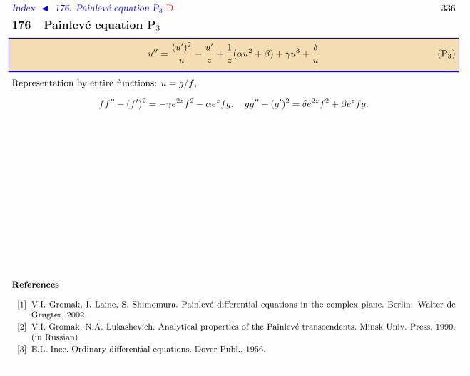
Index J 176. Painleve equation P3 D 336

176 Painleve equation P3

u′′ =(u′)2

u− u′

z+

1

z(αu2 + β) + γu3 +

δ

u(P3)

Representation by entire functions: u = g/f ,

ff ′′ − (f ′)2 = −γe2zf2 − αezfg, gg′′ − (g′)2 = δe2zf2 + βezfg.

References

[1] V.I. Gromak, I. Laine, S. Shimomura. Painleve differential equations in the complex plane. Berlin: Walter deGrugter, 2002.

[2] V.I. Gromak, N.A. Lukashevich. Analytical properties of the Painleve transcendents. Minsk Univ. Press, 1990.(in Russian)

[3] E.L. Ince. Ordinary differential equations. Dover Publ., 1956.

Index J 177. Painleve equation P4 D 337

177 Painleve equation P4

u′′ =(u′)2

2u+

3

2u3 + 4zu2 + 2(z2 − α)u+

β

u(P4)

Representation by entire functions: u = g/f ,

ff ′′ − (f ′)2 = −g(g + 2zf), (f ′g − fg′)2 − 4f ′f2g = g4 + 4zfg3 + 4(z2 − α)f2g2 − 2βf4.

References

[1] V.I. Gromak, I. Laine, S. Shimomura. Painleve differential equations in the complex plane. Berlin: Walter deGrugter, 2002.

[2] V.I. Gromak, N.A. Lukashevich. Analytical properties of the Painleve transcendents. Minsk Univ. Press, 1990.(in Russian)

[3] E.L. Ince. Ordinary differential equations. Dover Publ., 1956.

Index J 178. Painleve equation P5 D 338

178 Painleve equation P5

u′′ =

(1

2u+

1

u− 1

)(u′)2 − u′

z+

(u− 1)2

z2

(αu+

β

u

)+ γ

u

z+ δ

u(u+ 1)

u− 1(P5)

Representation by entire functions: u = g/f ,

ff ′′ − (f ′)2 = f(f ′ − g′)2 + 2αg(g − f),

(f ′g − fg′)2 = 2fg(f − g)(f ′ − g′) + 2(αg2 − βf2)(f − g)2 + 2γezf2g(f − g)− 2δe2zf2g2.

References

[1] V.I. Gromak, I. Laine, S. Shimomura. Painleve differential equations in the complex plane. Berlin: Walter deGrugter, 2002.

[2] V.I. Gromak, N.A. Lukashevich. Analytical properties of the Painleve transcendents. Minsk Univ. Press, 1990.(in Russian)

[3] E.L. Ince. Ordinary differential equations. Dover Publ., 1956.

Index J 179. Painleve equation P6 D 339

179 Painleve equation P6

u′′ =1

2

(1

u+

1

u− 1+

1

u− z

)(u′)2 −

(1

z+

1

z − 1+

1

u− z

)u′

+u(u− 1)(u− z)z2(z − 1)2

(α+ β

z

u2+ γ

z − 1

(u− 1)2+ δ

z(z − 1)

(u− z)2

)(P6)

References

[1] V.I. Gromak, I. Laine, S. Shimomura. Painleve differential equations in the complex plane. Berlin: Walter deGrugter, 2002.

[2] V.I. Gromak, N.A. Lukashevich. Analytical properties of the Painleve transcendents. Minsk Univ. Press, 1990.(in Russian)

[3] E.L. Ince. Ordinary differential equations. Dover Publ., 1956.

Index J 180. Painleve discrete equations ∆ 340

180 Painleve discrete equations

There exist a lot of nonautonomous difference equations which can be interpreted as discrete analogs ofPainleve equations. A comprehensive list can be found in [1]. Here we give several simplest examples.

Versions of dP1, accordingly to [2]:

an+ b

un+1 + un+a(n− 1) + b

un + un−1= c− u2

n (1)

un+1 + un + un−1 =an+ b

un+ c (2)

un+1 + un−1 =an+ b

un+

c

u2n

(3)

un+1 + un−1 =an+ b

un+ c (4)

un+1un−1 =ean+b

un+

c

u2n

(5)

Equation (2) was introduced in [3, 4].Versions of dP2:

un+1 + un−1 =(an+ b)un + a

u2n − 1

(6)

an+ b

unun+1 + 1+a(n− 1) + b

un−1un + 1=

1

un− un + an+ b+ c (7)

un+1un−1 = α1 + qn/un1 + qnun

(8)

Equation (6) was introduced in [5], in [6] the Miura-type transformation was found to the dP34:

(un+1 + un)(un + un−1) =m2 − 4u2

n

λun + nα+ β + (−1)nγ.

Index J 180. Painleve discrete equations ∆ 341

Alternate dP2 can be interpreted as nonlinear superposition principle for (P3) [2].dP4 [7, 8]:

(un+1 + un)(un + un−1) =(un + α+ β)(un + α− β)(un − α+ β)(un − α− β)

(un + δn+ ε+ γ)(un + δn+ ε− γ)

References

[1] B. Grammaticos, A. Ramani. Discrete Painleve equations: a review. Lect. Notes Phys. 644 (2004) 245–321.

[2] F.W. Nijhoff, J. Satsuma, K. Kajiwara, B. Grammaticos, A. Ramani. A study of the alternate discrete PainleveII equation. Inverse Problems 12 (1996) 697–716.

[3] E. Brezin, V. Kazakov. Phys. Lett. B 236 (1990) 144.

[4] A.R. Its, A.V. Kitaev, A.S. Fokas. The isomonodromy approach in the theory of two-dimensional quantumgravitation. Russ. Math. Surveys 45:6 (1987) 155–157.

[5] F.W. Nijhoff, V.G. Papageorgiou. Similarity reductions of integrable lattices and discrete analogues of PainlevePII equation. Phys. Lett. A 153:6–7 (1991) 337–344.

[6] A. Ramani, B. Grammaticos. Miura transforms for discrete Painleve equations. J. Phys. A 25:11 (1992) L633–637.

[7] A. Ramani, B. Grammaticos, J. Hietarinta. Discrete versions of the Painleve equations. Phys. Rev. Let. 67:14(1991) 1829–1832.

[8] J. Hietarinta, K. Kajiwara. Rational solutions to d-PIV. solv-int 9705002

Index J 181. Periodic closure 342

181 Periodic closure

Periodic boundary conditions turn infinite differential-difference equations into finite-dimensional dynam-ical systems. Typically, this preserves the integrability, since the lattice zero curvature representation istransformed into a finite-dimensional Lax representation:

Wn,x = Un+1Wn −WnUn, Un+N = Un ⇒ Wn,x = [Un, Wn], Wn = Wn+N−1 . . .Wn+1Wn

and the trace tr Wn becomes the generating function of the integrals of motion. Of course, the completenessof these integrals has to be proven for each example individually.

If the original lattice defines the Backlund auto-transformations of some equation then its periodic versiondefines some subclass of its solution. This possibility was proposed in the papers [1, 2], and then it wasshown [3] that in the case of Schrodinger operator this construction leads exactly to the finite-gap solutionsof KdV equation, see also [4].

The periodicity condition can be combined with any point transformation leaving the lattice invariant.In general, this spoils the integrability, and leads to the interesting examples which are exactly solvable inthe quantum-mechanical sense and are related to Painleve transcendents and their q-analogs [5, 3, 6].

ã Example. Following [3], consider the periodic solutions of the dressing chain:

f ′n + f ′n+1 = f2n − f2

n+1 + αn+1, n ∈ ZN , ε = −α1 − · · · − αN 6= 0. (1)

Under this reduction, applying of the operators A+n brings after N steps to the ψ-functions of the potential

shifted by ε. This means, assuming the regularity of potential and the suitable asymptotics of ψ-functions,that the spectrum of such potential consists of N arithmetic progressions. This is illustrated by the figurebelow corresponding to N = 3. The eigenfunctions of the operator Ln are constructed with the help ofmutually conjugated creation-annihilation operators of N -th order

A+n = A+

n . . . A+n+N−1, An = An+N−1 . . . An.

It is easy to prove that these operators satisfy the relations

A+n An = P (Ln), AnA

+n = P (Ln + ε), P (λ) = (λ− βn) . . . (λ− βn+N−1),

Index J 181. Periodic closure 343

[Ln, A+n ] = εA+

n , [Ln, An] = −εAn

which generalize the algebra of harmonic oscillator which corresponds to N = 1. Of course, the questionon the analytical properties of the system (1) solutions and the corre-sponding potentials and ψ-functions requires for an additional study.

-n

6λ

1 2 3

β1

β1 + ε

β2

β2 + ε

β3

β3 + ε

A+3

A+1 A+

2

A+1

q

q

q

q

q

q

q

q

q

q

q

q

q

qq

At N = 3, 4 the system (1) turns out to be equivalent to thePainleve equations P4 and P5 respectively. It is likely that at N ≥ 5the system possesses the Painleve property as well. However, forthe spectral theory the qualitative information is of most importanceabout the regularity of potential and its asymptotics. The relation2∑fn = −εx suggests that

fn = − εx

2N+O(1), un =

ε2x2

4N2+O(x), x→ ±∞.

At odd N , the numerical experiments demonstrate that this asymp-totics is true and the potential u1 is regular on the whole axis for arather large domain in the space of parameters and initial values of

the system. In such cases, it is easy to prove that formula (37.3) provides the eigenfunctions of the operatorL1. The value of ε on the presented plots is chosen ε = 2N , so that the leading asymptotic term is x2. Thechoice of initial values fn(0) = 0 provides the even potential u(−x) = u(x).

-6 -4 -2 2 4 6

x

10

20

30

40

50

u

-6 -4 -2 2 4 6

x

10

20

30

40

50

u

-6 -4 -2 2 4 6

x

10

20

30

40

50

u

N = 1 (harmonic oscillator) N = 3 (P4) N = 5

Index J 181. Periodic closure 344

For even N , the potentials have a singularity at x = 0 so that the proper spectral problem is formulatedon the halfline.

2 4 6 8 10

x

20

40

60

80

100

u

2 4 6 8 10

x

20

40

60

80

100

u

2 4 6 8 10

x

20

40

60

80

100

u

N = 2 (Kepler problem) N = 4 (P5) N = 6

References

[1] J. Weiss. Periodic fixed points of Backlund transformations and the Korteweg-de Vries equation. J. Math. Phys.27:11 (1986) 2647–2656.

[2] J. Weiss. Periodic fixed points of Backlund transformations. J. Math. Phys. 28:9 (1987) 2025–2039.

[3] A.P. Veselov, A.B. Shabat. Dressing chain and the spectral theory of Schrodinger operators. Funct. Anal. Appl.27:2 (1993) 81–96.

[4] A.P. Fordy, A.B. Shabat, A.P. Veselov. Factorisation and Poisson correspondences. Theor. Math. Phys. 105:2(1995) 1369–1386.

[5] A.B. Shabat. The infinite-dimensional dressing dynamical system. Inverse Problems 8 (1992) 303–308.

[6] V.E. Adler. Nonlinear chains and Painleve equations. Physica D 73:4 (1994) 335–351.

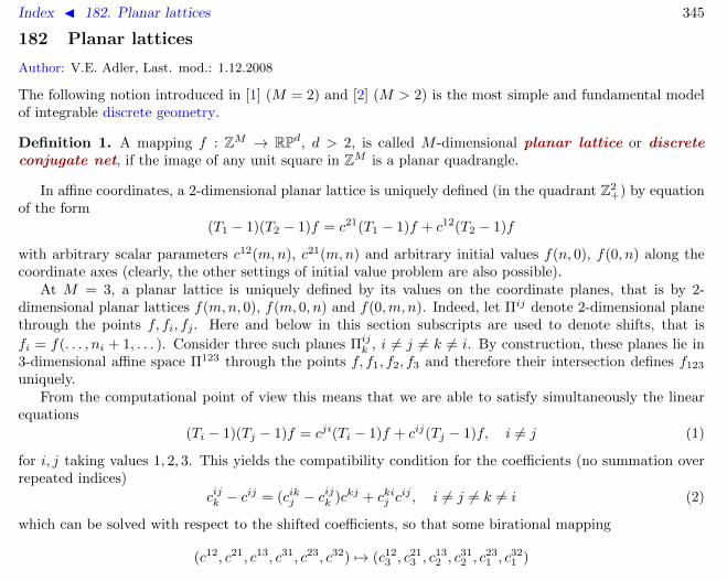
Index J 182. Planar lattices 345

182 Planar lattices

Author: V.E. Adler, Last. mod.: 1.12.2008

The following notion introduced in [1] (M = 2) and [2] (M > 2) is the most simple and fundamental modelof integrable discrete geometry.

Definition 1. A mapping f : ZM → RPd, d > 2, is called M -dimensional planar lattice or discreteconjugate net, if the image of any unit square in ZM is a planar quadrangle.

In affine coordinates, a 2-dimensional planar lattice is uniquely defined (in the quadrant Z2+) by equation

of the form

(T1 − 1)(T2 − 1)f = c21(T1 − 1)f + c12(T2 − 1)f

with arbitrary scalar parameters c12(m,n), c21(m,n) and arbitrary initial values f(n, 0), f(0, n) along thecoordinate axes (clearly, the other settings of initial value problem are also possible).

At M = 3, a planar lattice is uniquely defined by its values on the coordinate planes, that is by 2-dimensional planar lattices f(m,n, 0), f(m, 0, n) and f(0,m, n). Indeed, let Πij denote 2-dimensional planethrough the points f, fi, fj . Here and below in this section subscripts are used to denote shifts, that is

fi = f(. . . , ni + 1, . . . ). Consider three such planes Πijk , i 6= j 6= k 6= i. By construction, these planes lie in

3-dimensional affine space Π123 through the points f, f1, f2, f3 and therefore their intersection defines f123

uniquely.From the computational point of view this means that we are able to satisfy simultaneously the linear

equations

(Ti − 1)(Tj − 1)f = cji(Ti − 1)f + cij(Tj − 1)f, i 6= j (1)

for i, j taking values 1, 2, 3. This yields the compatibility condition for the coefficients (no summation overrepeated indices)

cijk − cij = (cikj − c

ijk )ckj + ckij c

ij , i 6= j 6= k 6= i (2)

which can be solved with respect to the shifted coefficients, so that some birational mapping

(c12, c21, c13, c31, c23, c32) 7→ (c123 , c

213 , c

132 , c

312 , c

231 , c

321 )

Index J 182. Planar lattices 346

arises. This mapping is rather cumbersome (it is written in [3], in a slightly different notation), but,fortunately, there exists a change of variables which brings it to a very nice form. Namely, alternating (2)with respect to i, k yields the relation

(cijk + 1)(ckj + 1) = (ckji + 1)(cij + 1)

which is solved by introducing the quantities hi (attached to the directed edges of the lattice) accordinglyto the formula

cij + 1 = hji/hj .

Now, introducing the vectors vi = (hi)−1(Ti − 1)f we bring the linear problem (1) to the form

(Ti − 1)vj = βjivi, βji :=(Tj − 1)hi

hji.

The new parameters βij are called discrete rotation coefficients. Their evolution is given by equations(see also [4])

βkji =βkj + βkiβij

1− βijβji, i 6= j 6= k 6= i. (3)

The important property of this evolution is that it can be correctly defined on the lattice of arbitrarydimension, so that the indices i, j, k may take arbitrary integer value and the commutativity property holdsβijkl = βijlk. In other words, the map βij → βijk is 4D-consistent. This can be easily verified directly, butmore simple and profound proof follows from the underlying geometric picture.

Theorem 2 (Doliwa, Santini). 3-dimensional planar lattices are 4D-consistent.

Proof. The initial data for a 4D cubic cell are vectors f, fi, fij , 1 ≤ i < j ≤ 4, such that fij ∈ Πij . Thisdefines f123 = Π12

3 ∩ Π132 ∩ Π23

1 and analogously for f124, f134 and f234. The value f1234 can be found asintersection Π12

34∩Π1324∩Π23

14, but obviously there are three more ways to do this. Therefore, we have to prove

that six planes Πijkl meet in one point. But Πij

kl = Πijkl ∩ Πijl

k , so that we have actually intersection of four3D spaces in 4D space Π1234 which give us a unique point.

Index J 182. Planar lattices 347

Notice, that this “general position” proof requires some modification in the case when all initial data lie insome 3D subspace (this may occur if the embedding dimension d = 3 or just as an accidental degeneration).This can be achieved by considering a 4D figure with the same 3D projection, like as in the proof of Desarguestheorem in a plane. Moreover, similar trick allows to define quadrilateral lattice also in the case d = 2 whenthe Definition 1 makes no sense: it is sufficient to require that this lattice be a projection of some lattice inRP3. A method to draw such projection effectively is given by the following theorem.

Theorem 3 ([5]). Consider a combinatorial cube on the plane. If, for some pair of the opposite faces, the(prolongations of) corresponding edges meet on a straight line, then the same is true for any other pair.

Proof. Collinearity of one quadruple of theintersection points allows to construct a com-binatorial cube in space, with planar faces, forwhich our figure is a projection. For such a fig-ure, edges meet on the intersections of 3 pairsof the planes.

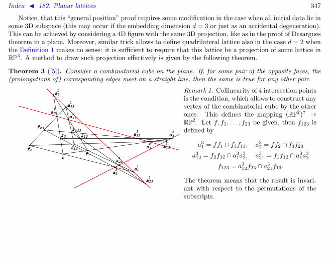
Index J 182. Planar lattices 347

Notice, that this “general position” proof requires some modification in the case when all initial data lie insome 3D subspace (this may occur if the embedding dimension d = 3 or just as an accidental degeneration).This can be achieved by considering a 4D figure with the same 3D projection, like as in the proof of Desarguestheorem in a plane. Moreover, similar trick allows to define quadrilateral lattice also in the case d = 2 whenthe Definition 1 makes no sense: it is sufficient to require that this lattice be a projection of some lattice inRP3. A method to draw such projection effectively is given by the following theorem.

Theorem 3 ([5]). Consider a combinatorial cube on the plane. If, for some pair of the opposite faces, the(prolongations of) corresponding edges meet on a straight line, then the same is true for any other pair.

ff1

f2f12

f3 f13

f23f123

a1

3

a2

3

a12

3

a21

3

a2

1

a3

1

a23

1

a32

1

a1

2

a3

2

a13

2

a31

2

Remark 1. Collinearity of 4 intersection pointsis the condition, which allows to construct anyvertex of the combinatorial cube by the otherones. This defines the mapping (RP2)7 →RP2. Let f, f1, . . . , f23 be given, then f123 isdefined by

a31 = ff1 ∩ f3f13, a3

2 = ff2 ∩ f3f23

a312 = f2f12 ∩ a3

1a32, a3

21 = f1f12 ∩ a31a

32

f123 = a312f23 ∩ a3

21f13.

The theorem means that the result is invari-ant with respect to the permutations of thesubscripts.

Index J 182. Planar lattices 347

Notice, that this “general position” proof requires some modification in the case when all initial data lie insome 3D subspace (this may occur if the embedding dimension d = 3 or just as an accidental degeneration).This can be achieved by considering a 4D figure with the same 3D projection, like as in the proof of Desarguestheorem in a plane. Moreover, similar trick allows to define quadrilateral lattice also in the case d = 2 whenthe Definition 1 makes no sense: it is sufficient to require that this lattice be a projection of some lattice inRP3. A method to draw such projection effectively is given by the following theorem.

Theorem 3 ([5]). Consider a combinatorial cube on the plane. If, for some pair of the opposite faces, the(prolongations of) corresponding edges meet on a straight line, then the same is true for any other pair.

Remark 2. Notice that all lines and pointsin the above figure are on equal footing.Namely, 8 vertices of the cube + 12 intersec-tion points and 12 sides + 3 lines of inter-sections form a regular configuration with thesymbol (203154). This configuration is men-tioned in [6], in connection with the followingstatement (equivalent to Theorem 3):

Let 3 triangles be perspective with thecommon center. Then 3 axes of perspective of3 pairs of triangles meet in one point.

Index J 182. Planar lattices 348

References

[1] R. Sauer. Differenzengeometrie. Berlin: Springer-Verlag, 1970.

[2] A. Doliwa, P.M. Santini. Multidimensional quadrilateral lattices are integrable. Phys. Lett. A 233:4–6 (1997)365–372.

[3] S.M. Sergeev. On exact solution of a classical 3D integrable model. J. Nonl. Math. Phys. 7:1 (2000) 57–72.

[4] L.V. Bogdanov, B.G. Konopelchenko. Lattice and q-difference Darboux–Zakharov–Manakov systems via ∂-dressing method. J. Phys. A 28:5 (1995) L173–178.

[5] V.E. Adler. Some incidence theorems and integrable discrete equations. Discrete Comput. Geom. 36 (2006)489–498.

[6] F. Levi. Geometrische Konfigurationen, Leipzig: 1929.

Index J 183. Plebanski equations d 349

183 Plebanski equations

first: uxyuzt − uxtuzy = 1 (1)

second: utx + uzy = u2xy − uxxuyy (2)

Alias: heavenly equation

References

[1] J.F. Plebanski. Some solutions of complex Einstein equations. J. Math. Phys. 16 (1975) 2395–2402.

[2] J.D.E. Grant. On self-dual gravity. Phys. Rev. D 48:6 (1993) 2606–2612.

[3] J.D.E. Grant, I.A.B. Strachan. Hypercomplex integrable systems. Nonlinearity 12 (1999) 1247–1261.

[4] E.V. Ferapontov, M.V. Pavlov. Hydrodynamic reductions of the heavenly equation. Class. Quantum Grav. 20(2003) 1–13.

Index J 184. Pohlmeyer–Lund–Regge system hDD 350

184 Pohlmeyer–Lund–Regge system

sxy + 〈sx, sy〉s = 0, s ∈ Rd, |s| = 1 (1)

Alias: O(n) σ-model

ã Due to the pseudo-constants |sx|y = 0, |sy|x = 0, the normalization

|sx| = |sy| = 1

can be achieved without loss of generality, by a change x→ x(x), y → y(y).

ã At d = 3, the substitution 〈sx, sy〉 = cosu brings to the sine-Gordon equation uxy = − sinu.

ã Similarly, at d = 4, the system appears [3]

uxy − sinu cosu+cosu

sin3 uvxvy = 0, (vy cot2 u)x + (vx cot2 u)y = 0. (2)

The reduction v = 0 brings to the sine-Gordon equation again. The system (2) can be cast to the rationalform

uxy =vuxuyuv + 1

+ u(uv + 1), vxy =uvxvyuv + 1

+ v(uv + 1) (3)

via the point transformation.

ã Backlund transformation for (3) [4]:

un,x = (unvn + 1)un+1, un,y = (unvn + 1)un−1

−vn,x = (unvn + 1)vn−1, −vn,y = (unvn + 1)vn+1

These lattices belong to the hierarchy of Ablowitz–Ladik lattice. Their higher symmetries bring to NLS-typesystems. This relation was studied also in [5].

Index J 184. Pohlmeyer–Lund–Regge system hDD 351

References

[1] K. Pohlmeyer. Integrable Hamiltonian systems and interaction through quadratic constraints. Commun. Math.Phys. 46:3 (1976) 207–218.

[2] F. Lund, T. Regge. Unified approach to strings and vortices with soliton solutions. Phys. Rev. D 14:6 (1976)1524–1535.

[3] F. Lund. Example of a relativistic, completely integrable, Hamiltonian system. Phys. Rev. Let. 38:21 (1977)1175–1178.

[4] A.B. Shabat, R.I. Yamilov. Symmetries of nonlinear chains. Len. Math. J. 2:2 (1991) 377–399.

[5] H. Aratyn, L.A. Ferreira, J.F. Gomes, A.H. Zimerman. The complex sine-Gordon equation as a symmetry flowof the AKNS hierarchy. J. Phys. A 33:35 (2000) L331–L337.

Index J 185. Pohlmeyer–Lund–Regge type systems hDD 352

185 Pohlmeyer–Lund–Regge type systems

uxy = f(ux, uy, u, v), vxy = g(vx, vy, v, u). (1)

Main examples are:

uxy = 2uvuy − u, vxy = −2uvvy − v (2)

uxy = h−1uxuy + h(1− uy), vxy = h−1vxvy + h(1 + vy), h = u+ v (3)

uxy = h−1ux(vuy − 1) + huy, vxy = h−1vx(uvy + 1)− hvy, h = uv + δ (4)

uxy = h−1vuxuy − uh, vxy = h−1uvxvy − vh, h = uv − 1 (5)

uxy = h−1(huuxuy + g(ux + uy) + gvh− ghv), vxy = h−1(hvvxvy − g(vx + vy) + guh− ghu),

g = hhuv − huhv, h(u, v) = h(v, u), huuu = 0(6)

ã The Pohlmeyer–Lund–Regge system [1, 2] itself is point equivalent to the system (5).

ã All above systems are Lagrangian, e.g. for the system (6) [4]:

L =

∫ ∫h−1(uxvy + huux − hvvy + g)dxdy.

ã The complex reductions are possible, e.g. the system (2) turns into

uxy = u− 2i|u|2uy

after the change ∂x → i∂x, ∂y → i∂y and under the reduction v = u.At h = const(u− v)2 the system (6) turns into

uxy =2uxuyu− v

− i(ux + uy), vxy =2vxvyv − u

+ i(vx + vy). (7)

ã The following theorem establishes the correspondence between the PLR type systems and the latticesgenerated by Backlund transformations for NLS type systems.

Index J 185. Pohlmeyer–Lund–Regge type systems hDD 353

Theorem 1. The systems (2)–(6) are obtained by elimination of the shifts from the following consistentpairs of the lattices (x+ = x, x− = y):

(2) :un,x = un+1 + u2

nvn, −vn,x = vn−1 + v2nun,

un,y =un−1

vnun−1 − 1, −vn,y =

vn+1

unvn+1 − 1

(3) :

un,x = (un + vn)(un+1 − un), −vn,x = (un + vn)(vn−1 − vn),

un,y =un + vnvn + un−1

, −vn,y =un + vnun + vn+1

(4) :

un,x = (unvn + δ)(un+1 + un), −vn,x = (unvn + δ)(vn−1 + vn),

un,y =un + un−1

vnun−1 − δ, −vn,y =

vn + vn+1

unvn+1 − δ(5) : un,x± = (unvn − 1)un±1, −vn,x± = (unvn − 1)vn∓1

(6) : un,x± =2h

un±1 − vn+ hvn , vn,x± =

2h

un − vn∓1− hun

, h = h(un, vn).

These formulae can be interpreted as explicit Backlund transformations for the PLR type systems. Forexample, for the system (2) one obtains the pair of auto-transformations (u, v)→ (u, v)±1

u1 = ux − u2v, v1 =vy

uvy + 1,

u−1 =uy

vuy − 1, v−1 = −vx − v2u,

which are mutually inverse in virtue of the system.

ã In conclusion, it should be noted that the full hierarchy of the higher symmetries for a PLR type systemconsists of two subhierarchies of NLS type, one contains the systems with x-derivatives, and another withthe y-derivatives. For example, the simplest higher symmetries of (2) are

ut1 = uxx − 2(u2vx + u3v2), −vt1 = vxx + 2(v2ux − v3u2)

Index J 185. Pohlmeyer–Lund–Regge type systems hDD 354

ut−1= uyy + 2u2

yvy, −vt−1= vyy − 2v2

yuy.

These are obtained by elimination of the shifts from the higher symmetries of the corresponding lattices.

References

[1] K. Pohlmeyer. Integrable Hamiltonian systems and interaction through quadratic constraints. Commun. Math.Phys. 46:3 (1976) 207–218.

[2] F. Lund, T. Regge. Unified approach to strings and vortices with soliton solutions. Phys. Rev. D 14:6 (1976)1524–1535.

[3] A.B. Shabat, R.I. Yamilov. Symmetries of nonlinear chains. Len. Math. J. 2:2 (1991) 377–399.

[4] V.E. Adler. Discretizations of the Landau–Lifshitz equation. Theor. Math. Phys. 124:1 (2000) 897–908.

[5] V.E. Adler, A.B. Shabat, R.I. Yamilov. Symmetry approach to the integrability problem. Theor. Math. Phys.125:3 (2000) 1603–1661.

[6] V.E. Adler, A.B. Shabat. On the one class of hyperbolic systems. SIGMA 2 (2006) 093.

Index J 186. Point transformations 355

186 Point transformations

Let u = (u1, . . . , um) and x = (x1, . . . , xn) be dependent and independent variables respectively. We will usethe multi-index notation us, s = (s1, . . . , sn) for the derivatives. A point transformation is defined by anarbitrary nondegenerate change

xi = fi(x, u), uj = gj(x, u). (1)

The prolongation of the transformation onto variables us is given by the formula

ujs = Ds(uj) = Ds11 · · · Dsn

n (uj), (2)

where operators Di are related with the operators of the total derivatives

Di = ∂xi+

m∑j=1

∑s

ujs+1i∂uj

s, 1i = (δ1,i, . . . , δn,i)

via the system of linear algebraic equations

Di(x1)D1 + · · ·+Di(xn)Dn = Di, i = 1, . . . , n. (3)

The determinant of this system does not vanish in virtue of the nondegeneracy of the transform (1). Moreover,equations (1), (2) define the invertible transformation on the set of the variables Jr = x, us : |s| =s1 + · · ·+ sn ≤ r for any r.

References

[1] L.V. Ovsyannikov. Group analysis of differential equations. New York: Academic Press, 1982.

[2] N.H. Ibragimov. Transformation groups applied to mathematical physics. Dordrecht: Reidel, 1985.

[3] P.J. Olver. Applications of Lie groups to differential equations, 2nd ed., Graduate Texts in Math. 107, NewYork: Springer-Verlag, 1993.

Index J 187. Quad-equations h∆∆ 356

187 Quad-equations

Author: V.E. Adler, 21.07.2005; Last mod. 3.12.2008

1. 3D-consistency2. List of quad-equations3. Zero curvature representation4. Three-leg form and discrete Toda lattices5. Multifield quad-equations

Quad-equation is a discrete equation on the lattice Z2, which relates the values of a field variable cor-responding to the vertices of any unit square. In a more general setup, the equations of quad-graphs areconsidered, that is on the planar graphs with quadrangle faces. Quad-equations appear as the nonlinearsuperposition principle for Backlund transformation. It is the commutativity of BTs what implies the 3D-consistency property and motivates the acceptance of this property as an intrinsic definition of integrabilityfor quad-equations.

1. 3D-consistency

Denote the vertices of the cube as shown on the picture and con-sider the system of 6 quad-equations associated to the faces of thecube (assuming uij := uji):

Qij(u, ui, uj , uij) = 0, Qij(uk, uik, ujk, u123) = 0.

This system is called 3D-consistent [1, 2], or consistent aroundthe cube, if the values u123 calculated in three possible ways co-incide for any choice of initial data u, u1, u2, u3.

0

1

2

12

3 13

13 123

• initial data• intermediate values• the results coincide

Index J 187. Quad-equations h∆∆ 356

187 Quad-equations

Author: V.E. Adler, 21.07.2005; Last mod. 3.12.2008

1. 3D-consistency2. List of quad-equations3. Zero curvature representation4. Three-leg form and discrete Toda lattices5. Multifield quad-equations

Quad-equation is a discrete equation on the lattice Z2, which relates the values of a field variable cor-responding to the vertices of any unit square. In a more general setup, the equations of quad-graphs areconsidered, that is on the planar graphs with quadrangle faces. Quad-equations appear as the nonlinearsuperposition principle for Backlund transformation. It is the commutativity of BTs what implies the 3D-consistency property and motivates the acceptance of this property as an intrinsic definition of integrabilityfor quad-equations.

1. 3D-consistency

Denote the vertices of the cube as shown on the picture and con-sider the system of 6 quad-equations associated to the faces of thecube (assuming uij := uji):

Qij(u, ui, uj , uij) = 0, Qij(uk, uik, ujk, u123) = 0.

This system is called 3D-consistent [1, 2], or consistent aroundthe cube, if the values u123 calculated in three possible ways co-incide for any choice of initial data u, u1, u2, u3.

0

1

2

12

3 13

13 123

• initial data• intermediate values• the results coincide

Index J 187. Quad-equations h∆∆ 356

187 Quad-equations

Author: V.E. Adler, 21.07.2005; Last mod. 3.12.2008

1. 3D-consistency2. List of quad-equations3. Zero curvature representation4. Three-leg form and discrete Toda lattices5. Multifield quad-equations

Quad-equation is a discrete equation on the lattice Z2, which relates the values of a field variable cor-responding to the vertices of any unit square. In a more general setup, the equations of quad-graphs areconsidered, that is on the planar graphs with quadrangle faces. Quad-equations appear as the nonlinearsuperposition principle for Backlund transformation. It is the commutativity of BTs what implies the 3D-consistency property and motivates the acceptance of this property as an intrinsic definition of integrabilityfor quad-equations.

1. 3D-consistency

Denote the vertices of the cube as shown on the picture and con-sider the system of 6 quad-equations associated to the faces of thecube (assuming uij := uji):

Qij(u, ui, uj , uij) = 0, Qij(uk, uik, ujk, u123) = 0.

This system is called 3D-consistent [1, 2], or consistent aroundthe cube, if the values u123 calculated in three possible ways co-incide for any choice of initial data u, u1, u2, u3.

0

1

2

12

3 13

13 123

• initial data• intermediate values• the results coincide

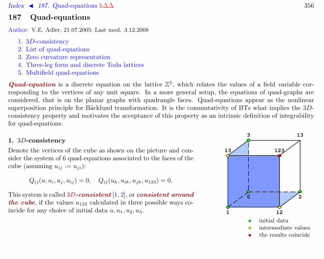
Index J 187. Quad-equations h∆∆ 357

Example 1. Discrete KdV equation

(u− uij)(ui − uj) = ai − aj , (uk − u123)(uik − ujk) = ai − aj

(parameter ai corresponds to 4 edges of the cube parallel to the edge (0, i)). One of the ways of computationyields

u12 = u− a1 − a2

u1 − u2, u13 = u− a1 − a3

u1 − u3,

u123 = u1 −a2 − a3

u12 − u13=a1u1(u2 − u3) + a2u2(u3 − u1) + a3u3(u1 − u2)

a1(u2 − u3) + a2(u3 − u1) + a3(u1 − u2).

Since this expression is symmetric with respect to the subscripts, two another ways give the same result.

Example 2. Linear equation

uij − ui − uj + u = 0, u123 − uik − ujk + uk = 0.

Independently on the order of computations u123 = u1 + u2 + u3 − 2u.

2. List of quad-equations

The classification of 3D-consistent equations has been obtained in [3] under the following assumptions:

ã Qij(u, ui, uj , uij) = Q(u, ui, uj , uij , ai, aj) where ai are parameters assigned to the edges parallel to (0, i);

ã function Q is affine-linear polynomial in u: Q = c1uu1u2u12 + · · ·+ c16 with coefficients depending on ai;

ã the equations admit the symmetry group of the square (ε2 = σ2 = 1):

Q(u, u1, u2, u12, a1α2) = εQ(u, u2, u1, u12, a2, a1) = σQ(u1, u, u12, u2, a1, a2); (1)

ã the tetrahedron condition: u123 as the function on initial data does not depend on u (cf examples 1,2).

Index J 187. Quad-equations h∆∆ 358

Theorem 3. Up to the simultaneous Mobius transformations of variables and point transformations ofparameters 3D-consistent equations satisfying the above assumptions are exhausted by the following list:

a1(u− u2)(u1 − u12)− a2(u− u1)(u2 − u12) = δ2a1a2(a2 − a1) (Q1)

a1(u− u2)(u1 − u12)− a2(u− u1)(u2 − u12) (Q2)

+ a1a2(a1 − a2)(u+ u1 + u2 + u12) = a1a2(a1 − a2)(a21 − a1a2 + a2

2)

(a22 − a2

1)(uu12 + u1u2) + a2(a21 − 1)(uu1 + u2u12)− a1(a2

2 − 1)(uu2 + u1u12) (Q3)

= δ2(a21 − a2

2)(a21 − 1)(a2

2 − 1)/(4a1a2)

sn a1 sn a2 sn(a1 − a2)(k2uu1u2u12 + 1) + sn a1(uu1 + u2u12) (Q4)

− sn a2(uu2 + u1u12)− sn(a1 − a2)(uu12 + u1u2) = 0, sn a ≡ sn(a; k)

(u− u12)(u1 − u2) = a1 − a2 (H1)

(u− u12)(u1 − u2) + (a2 − a1)(u+ u1 + u2 + u12) = a21 − a2

2 (H2)

a1(uu1 + u2u12)− a2(uu2 + u1u12) = δ(a22 − a2

1) (H3)

a1(u+ u2)(u1 + u12)− a2(u+ u1)(u2 + u12) = δ2a1a2(a1 − a2) (A1)

(a22 − a2

1)(uu1u2u12 + 1) = a1(a22 − 1)(uu1 + u2u12)− a2(a2

1 − 1)(uu2 + u1u12) (A2)

The proof is based on the relations between affine-linear, biquadratic and 4-th degree polynomials. Underthe imposed assumptions the relation holds

Qu2Qu12

−QQu2u12= k(a1, a2)h(u, u1, a1)

wherek(a2, a1) = −k(a1, a2), h(u1, u, a1) = h(u, u1, a1),

and moreover, the biquadratic h is such that the 4-th order polynomial

h2u1− 2hhu1u1

= r(u)

does not depend on the parameters of equation. After this, the classification is reduced to the problem ofreconstruction of h and Q starting from the polynomial r which can be brought to some canonical form byMobius transformations.

Index J 187. Quad-equations h∆∆ 359

Remark 4. ã Eq (A1) is reduced to (Q1) by the change ui → −ui; (A2) is reduced to (Q3) by the changeui → 1/ui.

ã Eqs (Q1)–(Q3) and (H1), (H2) can be obtained from (Q4), (H3) by degenerations and as limiting cases.

ã Eq (Q4) defines the nonlinear superposition principle for the Krichever–Novikov equation and is, in asense, the fundamental discrete equation [4].

ã The given form of (Q4) is found by Hietarinta [SIDE-2004 talk]. In [3] this equation was presented inmuch more cumbersome form related to the Weierstrass form of elliptic curve A2 = r(a) = 4a3 − g2a− g3.

ã The problem of classification without additional assumptions (affine-linearity, prescribed dependenceon parameters, symmetry, tetrahedron property) remains open. In particular, several examples withouttetrahedron property were found in [5]. It can be proved that the biquadratics h corresponding to suchequations are reducible.

ã Several equations are known with polynomial Q quadratic in each variable, but all these examples canbe reduced to affine-linear ones by Miura type transformations.

3. Zero curvature representation

An affine-linear equation Q = 0 may be interpreted as Mobius transformation between any pair of variables,with coefficients depending on the rest pair. Let

u13 = M(u1, u, a1, a3;u3) =Au3 +B

Cu3 +D

thenu23 = M(u2, u, a2, a3;u3), u123 = M(u12, u2, a1, a3;u23) = M(u12, u1, a2, a3;u13).

Since the composition of Mobius transformations corresponds to the product of the matrices, hence denotinga3 → λ and introducing the normalization factor yields the zero curvature representation

L(u12, u1, a2, λ)L(u1, u, a1, λ) = L(u12, u2, a1, λ)L(u2, u, a2, λ)

with the matrix

L(u1, u, a1, λ) = (AD −BC)−1/2

(A BC D

).

Index J 187. Quad-equations h∆∆ 360

For example, in the case of the discrete KdV equation (H1) one obtains

L(u1, u, a1, λ) =

(u −uu1 + a1 − λ1 −u1

).

4. Three-leg form and discrete Toda lattices

Let the quad-equation Q(u, u1, u2, u12, a1, a2) = 0 possesses the square symmetry (1). We will say that itadmits three-leg form if it is equivalent to the equation of the form

φ(u, u12, a1, a2) = ψ(u, u1, a1)− ψ(u, u2, a2).

Often it is convenient to use alternatively the multiplicative three-leg form

F (x, x12, α1 − α2) = F (x, x1, α1)/F (x, x2, α2).

Any three-leg equation corresponds to a discrete Toda lattice on a planar graph∑n

φ(u, un,n+1, an, an+1) = 0

where the sum is taken over the star of the vertex u.

Three-leg form exists for all equations from the above list, see the table. The general formula can beproved

ψ(u, u1, a1) =

∫du1

h(u, u1, a1)+ C(u, a1).

For the equations (Qn), a point change of parameters a = a(α) exists such that φ(u, u12, a1, a2) = ψ(u, u12, a(α1−α2)). Moreover, it is often convenient to make changes of the variables u = u(x) as well.

Index J 187. Quad-equations h∆∆ 361

F (x, y, α) u = u(x) a = a(α)

(Q1)δ=0 exp(α/(x− y)) x α

(Q1)δ=1x− y + α

x− y − αx α

(Q2)(x+ y + α)(x− y + α)

(x+ y − α)(x− y − α)x2 α

(Q3)δ=0sinh(x− y + α)

sinh(x− y − α)exp 2x exp 2α

(Q3)δ=1sinh(x+ y + α) sinh(x− y + α)

sinh(x+ y − α) sinh(x− y − α)cosh 2x exp 2α

(Q4)sn(x+ α)− sn y

sn(x− α)− sn y· Θ4(x+ α)

Θ4(x− α)snx α

(H1) :a1 − a2

u− u12= u1 − u2, (H2) :

u− u12 + a1 − a2

u− u12 − a1 + a2=u+ u1 + a1

u+ u2 + a2

(H3) :a2u− a1u12

a1u− a2u12=uu1 + δa1

uu2 + δa2

Remark 5. For the eq (Q4) with the polynomial r in Weierstrass form, the leg is

F =σ(x+ y + α)σ(x− y + α)

σ(x+ y − α)σ(x− y − α).

5. Multifield quad-equations

Classification of multifield analogs of quad-equations is hardly possible. One of the reasons is that theseequations are not polynomial, in contrast to the scalar case. Probably, the simplest example is the vector

Index J 187. Quad-equations h∆∆ 362

analog of the discrete KdV eq:

u− u12 =a1 − a2

|u1 − u2|2(u1 − u2).

This equation admits an interesting reduction ai = −|ui − u|2 [6]. Some other examples can be found in[7, 8].

The nonabelian analogs for the Krichever–Novikov equation (121.1) are known only for few special cases:

ã r = 0 Schwarz-KdV). The equation, its BT and NSP are

ut3 = uxxx −3

2uxxu

−1x uxx, ui,x = ai(u− ui)u−1

x (u− ui)

a1(u− u2)(u2 − u12)−1 = a2(u− u1)(u1 − u12)−1

ã r = 4

ut3 = uxxx −3

2uxxu

−1x uxx + 6u−1

x + 3[u−1x , uxx], ui,x =

1

ai(u− ui + ai)u

−1x (u− ui − ai)

a1(u1 − u12 + a2)(u− u1 − a1)−1 = a2(u2 − u12 + a1)(u− u2 − a2)−1

ã r = u2

ut3 = uxxx −3

2(uxxu

−1x uxx + uxxu

−1x u− uu−1

x uxx − uu−1x u)

ui,x =1

1− a2i

(u− aiui)u−1x (aiu− ui)

(1− a21)(u1 − a2u12)(a1u− u1)−1 = (1− a2

2)(u2 − a1u12)(a2u− u2)−1

These equations possess also 3-legs forms which lead to nonabelian discrete Toda type lattices.

Index J 187. Quad-equations h∆∆ 363

References

[1] F.W. Nijhoff, A.J. Walker. The discrete and continuous Painleve hierarchy and the Garnier system. GlasgowMath. J. 43A (2001) 109–123.

[2] A.I. Bobenko, Yu.B. Suris. Integrable systems on quad-graphs. Int. Math. Res. Notices (2002) 573–611.

[3] V.E. Adler, A.I. Bobenko, Yu.B. Suris. Classification of integrable equations on quad-graphs. The consistencyapproach. Commun. Math. Phys. 233 (2003) 513–543.

[4] V.E. Adler, Yu.B. Suris. Q4: Integrable master equation related to an elliptic curve. Int. Math. Res. Notices(2004) 2523–2553.

[5] J. Hietarinta. A new two-dimensional lattice model that is “consistent around a cube”. J. Phys. A 37:6 (2004)L67–73.

[6] V.E. Adler. Integrable deformations of a polygon. Physica D 87:1–4 (1995) 52–57.

[7] A.I. Bobenko, Yu.B. Suris. Integrable non-commutative equations on quad-graphs. The consistency approach.Lett. Math. Phys. 61 (2002) 241–254.

[8] W.K. Schief. Isothermic surfaces in spaces of arbitrary dimension: integrability, discretization and Backlundtransformations. A discrete Calapso equation. Stud. Appl. Math. 106:1 (2001) 85–137.

Index J 188. Quispel–Roberts–Thompson mapping ∆ 364

188 Quispel–Roberts–Thompson mapping

f3(un)un+1un−1 − f2(un)(un+1 + un−1) + f1(un) = 0, deg fi ≤ 4 (1)

Let A(u, v), B(u, v) be polynomials of degree 2 with respect to each variable:

A = a1u2v2 + · · ·+ a9, B = b1u

2v2 + · · ·+ b9.

Consider the mapping (un, vn)→ (un+1, vn+1) defined by equations

A(un, vn)

B(un, vn)=A(un, vn+1)

B(un, vn+1)=A(un+1, vn+1)

B(un+1, vn+1).

We have to solve a quadratic equation at each step, however one of the roots is already known and thereforea birational mapping appears. The quantity I = A/B is its invariant by construction and this provides theintegrability. The mapping (1) appears when the polynomials A,B are symmetric.

ã A particular case is the Euler–Chasles corrspondence (A is a symmetric polynomial and B = 1) [3, 4].The simplest and, historically, the first example is McMillan map [5]

References

[1] G.R.W. Quispel, J.A.G. Roberts, C.J. Thompson. Integrable mappings and soliton equations. Phys. Lett. A 126(1988) 419–421.

[2] G.R.W. Quispel, J.A.G. Roberts, C.J. Thompson. Integrable mappings and soliton equations: II. Physica D34:1–2 (1989) 183–192.

[3] A.P. Veselov. Integrable mappings. Russ. Math. Surveys 46:5 (1991) 1–51.

[4] A.P. Veselov. What is an integrable mapping? In: What is Integrability? (V.E. Zakharov ed). Springer-Verlag,1991, pp. 251–272.

[5] E.M. McMillan. A problem in the stability of periodic systems. In: Topics in Modern Physics. A tribute toE.U. Condon. (E. Britton, H. Odabasi eds) Boulder: Colorado Univ. Press, 1971, pp. 219–244.

[6] J.J. Duistermaat. QRT maps and elliptic surfaces. Springer-Verlag, 2009.

Index J 189. Recursion operator 365

189 Recursion operator

A differential or pseudo-differential operator R is called recursion operator [1] for an equation E = 0 if itmaps evolutionary symmetries of this equation into the evolutionary symmetries: G ∈ Sym(E) ⇒ R(G) ∈Sym(E).

ã In particular, if equation E is evolutionary itself, that is of the form ut = F , then equations utk = Rk(F ),k = 1, 2, 3, . . . should be its symmetries. In this case the recursion operator satisfies the equation

Rt = [F∗, R],

which coincides with the equation for the formal symmetry. The difference between these two notions is thatthe formal symmetry is in general an infinite series and its action on Sym(E) is not defined. In contrast,recursion operator must act on this set by definition. As a rule, the recursion operator is represented as aratio of differential operators R = JK−1, and it is necessary to prove that the result of its application tothe local symmetries is local again. See an example of such a proof for KdV equation.

The structure underlying the existence of recursion operator is given by Lenard–Magri scheme for theoperators J,K which constitute a bi-Hamiltonian pair).

ã See also: many examples of recursion operators are given in the corresponding articles, see e.g. Burgersequation, NLS system and so on.

References

[1] A.S. Fokas, B. Fuchssteiner. Symplectic structures, their Backlund transformations, and hereditary symmetries.Physica D 4:1 (1981) 47–66.

[2] P.J. Olver. Applications of Lie groups to differential equations, 2nd ed., Graduate Texts in Math. 107, NewYork: Springer-Verlag, 1993.

Index J 190. Reduction 366

190 Reduction

Reduction is the lowering of the number of dependent or independent variables by means of additionalconstraints. The most general method of finding the reductions is based on invariance of the system underscrutiny with respect to some subgroup of continuous or discrete symmetries.

Index J 191. Reyman system, twodimensional eDDD 367

191 Reyman system, twodimensional

ut = (ux + u2 − 2wx)x, vt = (−vx + 2uv)x, wy = v

ã Master-symmetry:

uτ = (x(ux + u2 − 2wx)− w)x, vτ = (x(−vx + 2uv)− v)x

ã Third order flow Dt3 = 12 [Dτ , Dt]:

ut3 = (uxx + 3uux + u3 − 3uwx − 3qx)x, vt3 = (vxx − 3uvx + 3u2v − 3vwx)x, qy = uv.

ã Auxiliary linear problems:

ψxy = uψy + vψ, ψT = A(x)ψxx − (2Awx +Axw)ψ

where A = 1 and A = x correspond to T = t and T = τ respectively. This is gauge equivalent to the linearproblem

ψy = Uφ, φx = −V ψ, u =UxU, v = −UV

for Davey–Stewartson system.

References

[1] V.E. Adler, A.B. Shabat, R.I. Yamilov. Symmetry approach to the integrability problem. Theor. Math. Phys.125:3 (2000) 1603–1661.

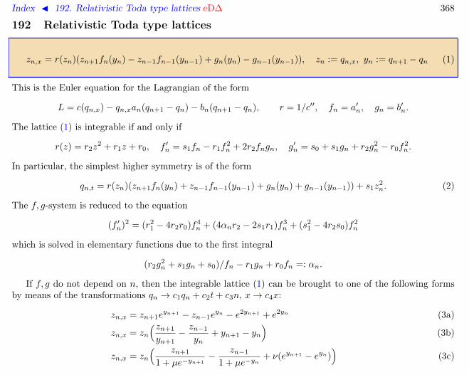
Index J 192. Relativistic Toda type lattices eD∆ 368

192 Relativistic Toda type lattices

zn,x = r(zn)(zn+1fn(yn)− zn−1fn−1(yn−1) + gn(yn)− gn−1(yn−1)), zn := qn,x, yn := qn+1 − qn (1)

This is the Euler equation for the Lagrangian of the form

L = c(qn,x)− qn,xan(qn+1 − qn)− bn(qn+1 − qn), r = 1/c′′, fn = a′n, gn = b′n.

The lattice (1) is integrable if and only if

r(z) = r2z2 + r1z + r0, f ′n = s1fn − r1f

2n + 2r2fngn, g′n = s0 + s1gn + r2g

2n − r0f

2n.

In particular, the simplest higher symmetry is of the form

qn,t = r(zn)(zn+1fn(yn) + zn−1fn−1(yn−1) + gn(yn) + gn−1(yn−1)) + s1z2n. (2)

The f, g-system is reduced to the equation

(f ′n)2 = (r21 − 4r2r0)f4

n + (4αnr2 − 2s1r1)f3n + (s2

1 − 4r2s0)f2n

which is solved in elementary functions due to the first integral

(r2g2n + s1gn + s0)/fn − r1gn + r0fn =: αn.

If f, g do not depend on n, then the integrable lattice (1) can be brought to one of the following formsby means of the transformations qn → c1qn + c2t+ c3n, x→ c4x:

zn,x = zn+1eyn+1 − zn−1e

yn − e2yn+1 + e2yn (3a)

zn,x = zn

(zn+1

yn+1− zn−1

yn+ yn+1 − yn

)(3b)

zn,x = zn

( zn+1

1 + µe−yn+1− zn−1

1 + µe−yn+ ν(eyn+1 − eyn)

)(3c)

Index J 192. Relativistic Toda type lattices eD∆ 369

zn,x = zn(zn + 1)(zn+1

yn+1− zn−1

yn

)(3d)

zn,x = zn(zn − µ)( zn+1

µ+ eyn+1− zn−1

µ+ eyn

)(3e)

zn,x = (z2n + µ)

(zn+1 − yn+1

µ+ y2n+1

− zn−1 − ynµ+ y2

n

)(3f)

zn,x =1

2(z2n + 1− µ2)

(zn+1 − sinh yn+1

µ+ cosh yn+1− zn−1 − sinh yn

µ+ cosh yn

)(3g)

References

[1] S.N.M. Ruijsenaars. Relativistic Toda system. Preprint Stichting Centre for Math. and Comp. Sciences, Ams-terdam, 1986.

[2] S.N.M. Ruijsenaars. Relativistic Toda systems. Commun. Math. Phys. 133:2 (1990) 217–247.

[3] V.E. Adler, A.B. Shabat. On a class of Toda chains. Theor. Math. Phys. 111:3 (1997) 647–657.

[4] V.E. Adler, A.B. Shabat. Generalized Legendre transformations. Theor. Math. Phys. 112:2 (1997) 935–948.

[5] V.E. Adler, A.B. Shabat, R.I. Yamilov. Symmetry approach to the integrability problem. Theor. Math. Phys.125:3 (2000) 1603–1661.

[6] V.E. Adler, A.B. Shabat. On the one class of hyperbolic systems. SIGMA 2 (2006) 093.

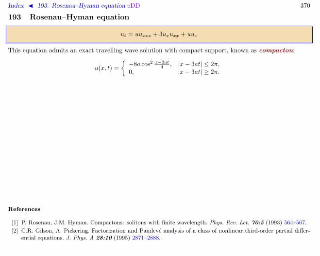
Index J 193. Rosenau–Hyman equation eDD 370

193 Rosenau–Hyman equation

ut = uuxxx + 3uxuxx + uux

This equation admits an exact travelling wave solution with compact support, known as compacton:

u(x, t) =

−8a cos2 x−3at

4 , |x− 3at| ≤ 2π,0, |x− 3at| ≥ 2π.

References

[1] P. Rosenau, J.M. Hyman. Compactons: solitons with finite wavelength. Phys. Rev. Let. 70:5 (1993) 564–567.

[2] C.R. Gilson, A. Pickering. Factorization and Painleve analysis of a class of nonlinear third-order partial differ-ential equations. J. Phys. A 28:10 (1995) 2871–2888.

Index J 194. Rosochatius system D 371

194 Rosochatius system

qk = pk = −ωkqk +µ2k

q3k

− qkN∑j=1

(q2j − ωjq2

j +µ2j

q2j

), 〈q, q〉 = 1, q = (q1, . . . , qN )ᵀ

ã The Poisson structure is defined as the Dirac reduction of the canonical bracket to the level set 〈q, q〉 = 1,〈q, p〉 = 0:

qk, qj = 0, pk, qj = δkj − qkqj , pk, pj = qkpj − qjpk, H =1

2

N∑k=1

(p2k + ωkq

2k +

µ2k

q2k

).

The N − 1 independent first integrals in involution (assuming ωk 6= ωj , ∀ k, j) are:

Fk = q2k +

∑j 6=k

1

ωk − ωj

((pkqj − pjqk)2 +

µ2kq

2j

q2k

+µ2jq

2k

q2j

),

N∑k=1

Fk = 〈q, q〉 = 1,

N∑k=1

ωkFk = H.

ã Lax pair L = [M,L]:

L = −diag(ω1, . . . , ωN ) + λ

(pqᵀ − qpᵀ + i

µ

qqᵀ + iq

(µq

)ᵀ)+ λ2qqᵀ, M = λqqᵀ + idiag

(µ1

q21

, . . . ,µNq2N

)where p, q,

µ

qare column vectors with the k-th entry pk, qk,

µkqk

respectively.

ã See also Wojciechowski system

References

[1] E. Rosochatius. Uber die Bewegung eines Punktes. Inaugural dissertation, Berlin, 1877.

Index J 194. Rosochatius system D 372

[2] J. Moser. Geometry of quadrics and spectral theory. Chern symposium (1979) 147.

[3] T. Ratiu. The Lie-algebraic interpretation of the complete integrability of the Rosochatius system. Math. Methodsin Hydrodynamics and Integrability in Dynamical Systems, American Institute of Physics, (1982) 108.

[4] Yu.B. Suris. Dynamical r-matrices for some nonlinear oscillators. J. Phys. A 28:3 (1995) L85–90.

[5] Yu.B. Suris. The problem of integrable discretization: Hamiltonian approach. Basel: Birkhauser, 2003.

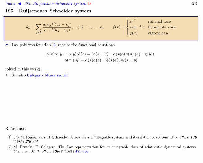
Index J 195. Ruijsenaars–Schneider system D 373

195 Ruijsenaars–Schneider system

uk =∑j 6=k

ukujf′(uk − uj)

c− f(uk − uj), j, k = 1, . . . , n, f(x) =

x−2 rational case

sinh−2 x hyperbolic case

℘(x) elliptic case

ã Lax pair was found in [2] (notice the functional equations

α(x)α′(y)− α(y)α′(x) = (α(x+ y)− α(x)α(y))(η(x)− η(y)),

α(x+ y) = α(x)α(y) + φ(x)φ(y)ψ(x+ y)

solved in this work).

ã See also Calogero–Moser model

References

[1] S.N.M. Ruijsenaars, H. Schneider. A new class of integrable systems and its relation to solitons. Ann. Phys. 170(1986) 370–405.

[2] M. Bruschi, F. Calogero. The Lax representation for an integrable class of relativistic dynamical systems.Commun. Math. Phys. 109:3 (1987) 481–492.

Index J 196. Sawada–Kotera equation eDD 374

196 Sawada–Kotera equation

ut = u5 + 5uu3 + 5u1u2 + 5u2u1 (1)

ã Generic 3rd and 5th order operators L,A satisfying the Lax equation Lt = [A,L] can be brought to theform

L = D3x + uDx + v, −A = 9D5

x + 15uD3x + 15(u1 + v)D2

x + 5(2u2 + u2 + 3v1)Dx + 10(v2 + uv),

with u, v governed by the system

ut = u5 + 5(uu2 + 3v(u1 − v) +1

3u3)x,

vt = v5 + 5(uv2 + 2u2v + 2u1v1 − 3vv1 + u2v)x.

This system admits the reductions:v = 0, v = ux both corresponding to equation (1);2v = ux corresponding to Kaup–Kupershmidt equation.

ã Backlund transformation (u = 6wx):

(w − w)xx + 3(w − w)(w + w)x + (w − w)3 = β

References

[1] K. Sawada, T. Kotera. A method for finding n-soliton solutions of the KdV equation and KdV-like equations.Progr. Theor. Phys. 51 (1974) 1355–1367.

[2] D.J. Kaup. On the inverse scattering problem for cubic eigenvalue problems of the class ψxxx+6Qψx+6Rψ = λψ.SIAM J. on Appl. Math. 62 (1980) 189–216.

[3] P.J. Caudrey, R.K. Dodd, J.D. Gibbon. A new hierarchy of Korteweg-de Vries equations. Proc. Roy. Soc. LondonA 351 (1976) 407–422.

[4] V.G. Drinfeld, V.V. Sokolov. Lie algebras and equations of Korteweg-de Vries type. J. Soviet Math. 30 (1985)1975–2036.

Index J 197. Sawada–Kotera equation, twodimensional eDD 375

197 Sawada–Kotera equation, twodimensional

ut = u5 + 5uu3 + 5u1u2 + 5u2u1 − 5u2,y − 5uuy − 5u1w − 5wy, uy = wx (1)

ã Introduced in [1].

ã Consider auxiliary linear problems ψy = Lψ, ψt = Aψ. Generic 3rd and 5th order operators L,A can bebrought to the form

L = D3x + uDx + v, −A = 9D5

x + 15uD3x + 15(u1 + v)D2

x + 5(2u2 + u2 + 3v1 + w)Dx + 5(2v2 + 2uv + s),

with u, v governed by the system

ut = u5 + 5(uu2 + 3v(u1 − v) +1

3u3)x − 5(u2,y + uuy + u1w + wy), uy = wx,

vt = v5 + 5(uv2 + 2u1v1 + 2u2v − 3vv1 + u2v)x − 5(v2,y + 2vuy + uvy + v1w + sy), vy = sx.

This system admits the reductions:v = 0, s = 0 and v = ux, s = ux both corresponding to 2D-SK equation (1);2v = ux, 2s = uy corresponding to 2D Kaup–Kupershmidt equation.

References

[1] B.G. Konopelchenko, V.G. Dubrovsky. Some new integrable nonlinear evolution equations in 2 + 1 dimensions.Phys. Lett. A 102:1–2 (1984) 15–17.

Index J 198. Selfsimilar solutions 376

198 Selfsimilar solutions

Selfsimilar solution of a PDE or D∆E is a special solution characterized by its invariance with respect tosome subgroup of the Lie group of classical symmetries of the equation [1, 2, 3].

In the most common situations selfsimilar solutions are invariant with respect to some shift or dilationtransformation. In many physical models such solutions define the asymptotic behaviour of the generalsolutions.

The construction of the selfsimilar solutions amounts to solving of the equation for the invariants ofthe subgroup. This reduces the dimensionality of the problem, for example, the selfsimilar solutions of anequation with two independent variables are defined by some ODEs. If the original equation was integrablethen, accordingly to the Ablowitz–Ramani–Segur conjecture, these ODEs possess the Painleve property.

References

[1] L.V. Ovsyannikov. Group analysis of differential equations, New York: Academic Press, 1982.

[2] N.H. Ibragimov. Transformation groups applied to mathematical physics. Dordrecht: Reidel, 1985.

[3] P.J. Olver. Applications of Lie groups to differential equations, 2nd ed., Graduate Texts in Math. 107, NewYork: Springer-Verlag, 1993.

Index J 199. Shabat equation Dq 377

199 Shabat equation

q2v′(qx) + v′(x) = (qv(qx)− v(x))2 − 1, v(0) = α (1)

ã This ODE with proportional delay arises as the self-similar reduction of the dressing chain. Its solution isunique in the class of meromorphic function in C. The spectrum of the corresponding Schrodinger operatorwith the potential u = 2v′ consists of the infinite geometric progression −q2n, n = 0, 1, . . . [2, 3].

ã The analytic properties of the solution were studied in [4, 5, 6]. Rational solutions, corresponding to thespecial values of α were constructed in [7]. Some generalizations corresponding to selfsimilar closure of thedressing chain after several steps were discussed in [8].

References

[1] A.B. Shabat. The infinite-dimensional dressing dynamical system. Inverse Problems 8 (1992) 303–308.

[2] A. Degasperis, A.B. Shabat. Construction of reflectionless potentials with infinitely many discrete eigenvalues.in: Applications of analytic and geometric methods to nonlinear differential equations. (P.A. Clarkson ed) NATOAdvanced Study Institute Series C: Math. and Phys. Sci. 413, Dordrecht: Kluwer, 1993.

[3] A. Degasperis, A.B. Shabat. Construction of reflectionless potentials with infinite discrete spectra. Theor. Math.Phys. 100:2 (1994) 970–984

[4] Yunkang Liu. On functional differential equations with proportional delays. Ph. D. Thesis, Cambridge University,1996.

[5] Yunkang Liu. Regular solutions of the Shabat equation. J. Diff. Eq. 154 (1999) 1–41.

[6] Yunkang Liu. An existence result for the Shabat equation. Aeq. Math. 64 (2002) 104–109.

[7] V.E. Adler. On the rational solutions of the Shabat equation. Proc. of Int. Workshop ’Nonlinear Physics’, pp.53–61, World Scientific, 1996.

[8] S. Skorik, V. Spiridonov. Self-similar potentials and the q-oscillator algebra at roots of unity. Lett. Math. Phys.28 (1993) 59–74.

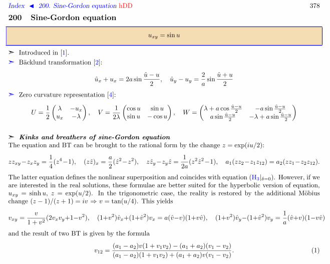
Index J 200. Sine-Gordon equation hDD 378

200 Sine-Gordon equation

uxy = sinu

ã Introduced in [1].

ã Backlund transformation [2]:

ux + ux = 2a sinu− u

2, uy − uy =

2

asin

u+ u

2

ã Zero curvature representation [4]:

U =1

2

(λ −uxux −λ

), V =

1

2λ

(cosu sinusinu − cosu

), W =

(λ+ a cos u−u2 −a sin u−u

2

a sin u−u2 −λ+ a sin u−u

2

)

ã Kinks and breathers of sine-Gordon equationThe equation and BT can be brought to the rational form by the change z = exp(iu/2):

zzxy−zxzy =1

4(z4−1), (zz)x =

a

2(z2−z2), zzy−zy z =

1

2a(z2z2−1), a1(zz2−z1z12) = a2(zz1−z2z12).

The latter equation defines the nonlinear superposition and coincides with equation (H3|δ=0). However, if weare interested in the real solutions, these formulae are better suited for the hyperbolic version of equation,uxy = sinhu, z = exp(u/2). In the trigonometric case, the reality is restored by the additional Mobiuschange (z − 1)/(z + 1) = iv ⇒ v = tan(u/4). This yields

vxy =v

1 + v2(2vxvy+1−v2), (1+v2)vx+(1+v2)vx = a(v−v)(1+vv), (1+v2)vy−(1+v2)vy =

1

a(v+v)(1−vv)

and the result of two BT is given by the formula

v12 =(a1 − a2)v(1 + v1v2)− (a1 + a2)(v1 − v2)

(a1 − a2)(1 + v1v2) + (a1 + a2)v(v1 − v2). (1)

Index J 200. Sine-Gordon equation hDD 379

Applying the BT to the seed solution u = 0 we obtain immediately the kink solution

v = tan(u/4) = c exp(ax+ y/a),

and the formula (1) allows to construct the multi-kinks. The general formula for 2-kink solution is

tanu

4=

(a1 + a2)(c2 exp(a2x+ y/a2)− c1 exp(a1x+ y/a1))

(a1 − a2)(1 + c1c2 exp((a1 + a2)x+ y(1/a1 + 1/a2))).

The solution v12 remains real if the intermediate solutions v1, v2 are complex conjugate. In particular,assuming in the above solution a1 = α+ iβ, a2 = α− iβ and c1 = c2 we come to the breather solution

tanu

4=

α sin(β(x− y/γ) + φ1)

β cosh(α(x+ y/γ) + φ2), γ = α2 + β2.

-15 -10 -5 5 10 15x

Π

2 Π

u

-10

0

10

x-5

0

5

y

-5

0

5

u

-10

0

10

x

-10

0

10

x-5

0

5

y

-5

0

5

u

-10

0

10

x

one-kink profile kink-antikink solution two-kink solutiona = 0.5, c = 1, y = 0 a1 = 0.5, a2 = 1, c1 = c2 = 0 a1 = 0.5, a2 = −1, c1 = c2 = 0

Index J 200. Sine-Gordon equation hDD 380

-15 -10 -5 5 10 15

x

-1

-0.5

0.5

1

u

-10

0

10x -5

0

5

y

-2-1

0123

u

-10

0

10x

breather profile (t = 0) α = 0.5, β = 1.5, φ1 = φ2 = 0

References

[1] E. Bour. Theorie de la deformation des surfaces. J. l’Ecole Imp. Polytech. 19:39 (1862) 1–48.

[2] A.V. Backlund. Om ytor med konstant negativ krokning. Lunds Universitets Arsskrift 19 (1883) 1–48.

[3] L. Bianchi. Sulla trasformazione di Backlund per le superficie pseudosferiche. Rend. Ac. Naz. dei Lincei 5 (1892)3–12.

[4] M.J. Ablowitz, D.J. Kaup, A.C. Newell, H. Segur. Method for solving the sine-Gordon equation. Phys. Rev. Let.30:25 (1973) 1262–1264.

Index J 201. Sine-Gordon equation, double hDD 381

201 Sine-Gordon equation, double

uxt = sinu+ a sinu

2

References

[1] R.K. Dodd, J.C. Eilbeck, J.D. Gibbon, H.C. Morris. Solitons and nonlinear wave equations. London: AcademicPress, 1982.

[2] J. Weiss. The sine-Gordon equation: complete and partial integrability. J. Math. Phys. 25:7 (1984) 2226–2235.

Index J 202. Sine-Gordon equation, multidimensional hND 382

202 Sine-Gordon equation, multidimensional

ux1x1 + · · ·+ uxnxn = sinu

References

[1] J. Weiss. The sine-Gordon equation: complete and partial integrability. J. Math. Phys. 25:7 (1984) 2226–2235.

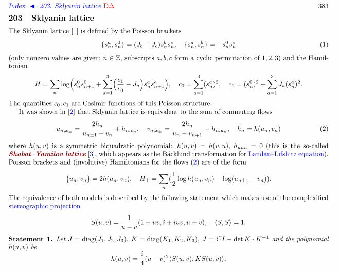
Index J 203. Sklyanin lattice D∆ 383

203 Sklyanin lattice

The Sklyanin lattice [1] is defined by the Poisson brackets

san, s0n = (Jb − Jc)sbnscn, san, sbn = −s0

nscn (1)

(only nonzero values are given; n ∈ Z, subscripts a, b, c form a cyclic permutation of 1, 2, 3) and the Hamil-tonian

H =∑n

log(s0ns

0n+1 +

3∑a=1

(c1c0− Ja

)sans

an+1

), c0 =

3∑a=1

(san)2, c1 = (s0n)2 +

3∑a=1

Ja(san)2.

The quantities c0, c1 are Casimir functions of this Poisson structure.It was shown in [2] that Sklyanin lattice is equivalent to the sum of commuting flows

un,x± =2hn

un±1 − vn+ hn,vn , vn,x± =

2hnun − vn∓1

− hn,un, hn = h(un, vn) (2)

where h(u, v) is a symmetric biquadratic polynomial: h(u, v) = h(v, u), huuu = 0 (this is the so-calledShabat–Yamilov lattice [3], which appears as the Backlund transformation for Landau–Lifshitz equation).Poisson brackets and (involutive) Hamiltonians for the flows (2) are of the form

un, vn = 2h(un, vn), H± =∑n

(1

2log h(un, vn)− log(un±1 − vn)).

The equivalence of both models is described by the following statement which makes use of the complexifiedstereographic projection

S(u, v) =1

u− v(1− uv, i+ iuv, u+ v), 〈S, S〉 = 1.

Statement 1. Let J = diag(J1, J2, J3), K = diag(K1,K2,K3), J = CI − detK ·K−1 and the polynomialh(u, v) be

h(u, v) =i

4(u− v)2〈S(u, v),KS(u, v)〉.

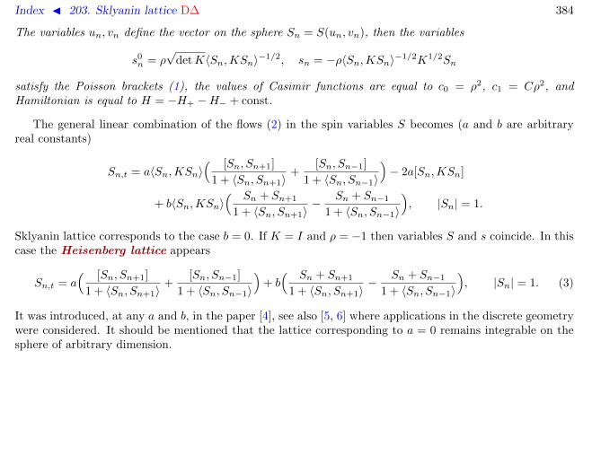
Index J 203. Sklyanin lattice D∆ 384

The variables un, vn define the vector on the sphere Sn = S(un, vn), then the variables

s0n = ρ

√detK〈Sn,KSn〉−1/2, sn = −ρ〈Sn,KSn〉−1/2K1/2Sn

satisfy the Poisson brackets (1), the values of Casimir functions are equal to c0 = ρ2, c1 = Cρ2, andHamiltonian is equal to H = −H+ −H− + const.

The general linear combination of the flows (2) in the spin variables S becomes (a and b are arbitraryreal constants)

Sn,t = a〈Sn,KSn〉( [Sn, Sn+1]

1 + 〈Sn, Sn+1〉+

[Sn, Sn−1]

1 + 〈Sn, Sn−1〉

)− 2a[Sn,KSn]

+ b〈Sn,KSn〉( Sn + Sn+1

1 + 〈Sn, Sn+1〉− Sn + Sn−1

1 + 〈Sn, Sn−1〉

), |Sn| = 1.

Sklyanin lattice corresponds to the case b = 0. If K = I and ρ = −1 then variables S and s coincide. In thiscase the Heisenberg lattice appears

Sn,t = a( [Sn, Sn+1]

1 + 〈Sn, Sn+1〉+

[Sn, Sn−1]

1 + 〈Sn, Sn−1〉

)+ b( Sn + Sn+1

1 + 〈Sn, Sn+1〉− Sn + Sn−1

1 + 〈Sn, Sn−1〉

), |Sn| = 1. (3)

It was introduced, at any a and b, in the paper [4], see also [5, 6] where applications in the discrete geometrywere considered. It should be mentioned that the lattice corresponding to a = 0 remains integrable on thesphere of arbitrary dimension.

Index J 203. Sklyanin lattice D∆ 385

References

[1] E.K. Sklyanin. On some algebraic structures related to Yang–Baxter equation. Funct. Anal. Appl. 16:4 (1982)27–34.

[2] V.E. Adler. Discretizations of the Landau–Lifshitz equation. Theor. Math. Phys. 124:1 (2000) 897–908.

[3] A.B. Shabat, R.I. Yamilov. Symmetries of nonlinear chains. Len. Math. J. 2:2 (1991) 377–399.

[4] O. Ragnisco, P.M. Santini. A unified algebraic approach to integral and discrete evolution equations. InverseProblems 6:3 (1990) 441–452.

[5] A.I. Bobenko. Discrete integrable systems and geometry. In: XIIth Int. Congress of Math. Phys. (ICMP’97,Brisbane), 219–226, Cambridge: Internat. Press, 1999.

[6] A.I. Bobenko, Yu.B. Suris. Discrete time Lagrangian mechanics on Lie groups, with an application to theLagrange top. Commun. Math. Phys. 204:1 (1999) 147–188.

Index J 204. Short Pulse equation hDD 386

204 Short Pulse equation

vyt = v +1

6(v3)yy

ã The differential substitution to sine-Gordon equation uxt = sinu [5]:

v = ut, dy = cosu dx− 1

2u2tdt.

ã Zero curvature representation

Ψy =1

2λ

(1 vyvy −1

), Ψt =

v2

2U +

1

2

(λ −vv −λ

).

ã Higher symmetry [7]:

vt3 =

(vyy

(1 + v2y)3/2

)y

References

[1] R. Beals, M. Rabelo, K. Tenenblat. Backlund transformations and inverse scattering solutions for some pseudo-spherical surface equations. Stud. Appl. Math. 81 (1989) 125–151.

[2] M.L. Rabelo. On equations which describe pseudospherical surfaces. Stud. Appl. Math. 81 (1989) 221–248.

[3] T. Schafer, C.E. Wayne. Propagation of ultra-short optical pulses in cubic nonlinear media. Physica D 196(2004) 90–105.

[4] Y. Chung, C.K.R.T. Jones, T. Schafer, C.E. Wayne. Ultra-short pulses in linear and nonlinear media. Nonlin-earity 18 (2005) 1351–1374.

[5] A. Sakovich, S. Sakovich. The short pulse equation is integrable. J. Phys. Soc. Jpn. 74 (2005) 239–241.

[6] J.C. Brunelli. The bi-Hamiltonian structure of the short pulse equation. Phys. Lett. A 353:6 (2006) 475–478.

[7] J.C. Brunelli. The short pulse hierarchy. J. Math. Phys. 46 (2005) 123507.

Index J 205. Soliton solutions 387

205 Soliton solutions

Many nonlinear PDEs admit particular exact solutions in the form of localized travelling waves, as a rulewith the amplitude depending on the velocity:

u(x, t) = A(k)f(kx+ ω(k)t+ δ;α), f(x;α)→ 0, x→ ±∞.

Here α denote additional parameters, such as polarization. The profile of the wave f , the amplitude A anddispersion law ω depend on the form of equation. Such solutions are called solitary waves. In general,the collision of two solitary waves leads to their destruction or to appearance of small oscillations. However,several equations admit exact solutions which represent an elastic interaction of arbitrarily many solitarywaves. Such solutions are called multi-soliton solutions [1].

More rigorously, the solution is called N-soliton if it is asymptotically equal to the sum of N localizedtravelling waves which interact without changing their shapes, amplitudes and velocities, so that the onlyresult of interaction is the shifts of the phases and, possibly, some parameters:

u(x, t) ∼N∑i=1

A(ki)f(kix+ ω(ki)t+ δ±i ;α±i ), t→ ±∞.

There exist equations which admit 2-soliton solutions but cannot support 3-soliton one. However, in allknown examples, the existence of 3-soliton solution implies the existence of N -soliton one for any N .

In some cases this definition appears too restrictive. For example, the number of solitons may changedin the 3-wave interaction.

ã See also: KdV solitons

References

[1] N.J. Zabusky, M.D. Kruskal. Interaction of “solitons” in a collisionless plasma and the recurrence of initialstates. Phys. Rev. Let. 15:6 (1965) 240–243.

Index J 206. Somos sequences ∆ 388

206 Somos sequences

S4 : anan−4 = an−1an−3 + a2n−2, a0 = · · · = a3 = 1

S5 : anan−5 = an−1an−4 + an−2an−3, a0 = · · · = a4 = 1

S6 : anan−6 = an−1an−5 + an−2an−4 + a2n−2, a0 = · · · = a5 = 1

S7 : anan−7 = an−1an−6 + an−2an−5 + an−3an−4, a0 = · · · = a6 = 1

These recurrent relations generate integers for any n. In a more general setting, an are Laurent polynomialson the initial data a0, . . . , ak−1 for Sk. This is the so-called Laurent property which is observed for someother discrete equations as well. However, it is not valid for the higher sequences Sk at k > 7.

References

[1] D. Gale. The strange and surprising saga of the Somos sequences. Math. Intell. 13 (1991) 40–42.

[2] D. Gale. Somos sequence update. Math. Intell. 13 (1991) 49–50.

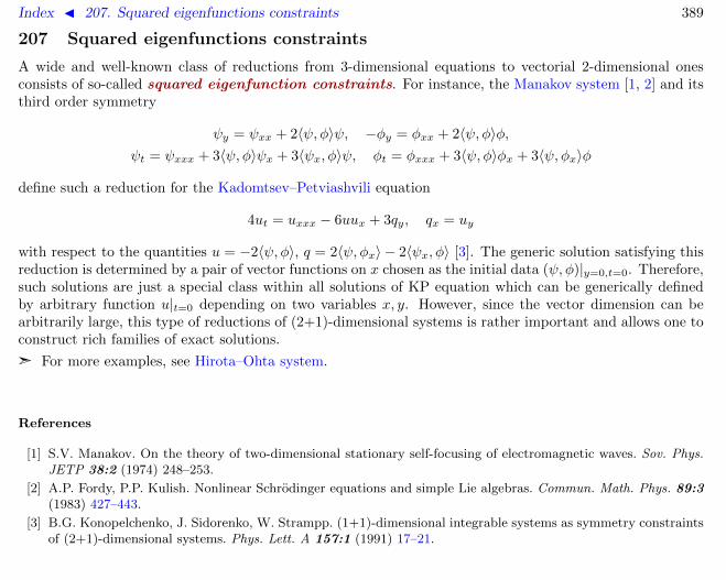
Index J 207. Squared eigenfunctions constraints 389

207 Squared eigenfunctions constraints

A wide and well-known class of reductions from 3-dimensional equations to vectorial 2-dimensional onesconsists of so-called squared eigenfunction constraints. For instance, the Manakov system [1, 2] and itsthird order symmetry

ψy = ψxx + 2〈ψ, φ〉ψ, −φy = φxx + 2〈ψ, φ〉φ,ψt = ψxxx + 3〈ψ, φ〉ψx + 3〈ψx, φ〉ψ, φt = φxxx + 3〈ψ, φ〉φx + 3〈ψ, φx〉φ

define such a reduction for the Kadomtsev–Petviashvili equation

4ut = uxxx − 6uux + 3qy, qx = uy

with respect to the quantities u = −2〈ψ, φ〉, q = 2〈ψ, φx〉 − 2〈ψx, φ〉 [3]. The generic solution satisfying thisreduction is determined by a pair of vector functions on x chosen as the initial data (ψ, φ)|y=0,t=0. Therefore,such solutions are just a special class within all solutions of KP equation which can be generically definedby arbitrary function u|t=0 depending on two variables x, y. However, since the vector dimension can bearbitrarily large, this type of reductions of (2+1)-dimensional systems is rather important and allows one toconstruct rich families of exact solutions.

ã For more examples, see Hirota–Ohta system.

References

[1] S.V. Manakov. On the theory of two-dimensional stationary self-focusing of electromagnetic waves. Sov. Phys.JETP 38:2 (1974) 248–253.

[2] A.P. Fordy, P.P. Kulish. Nonlinear Schrodinger equations and simple Lie algebras. Commun. Math. Phys. 89:3(1983) 427–443.

[3] B.G. Konopelchenko, J. Sidorenko, W. Strampp. (1+1)-dimensional integrable systems as symmetry constraintsof (2+1)-dimensional systems. Phys. Lett. A 157:1 (1991) 17–21.

Index J 208. The symmetry approach 390

208 The symmetry approach

Author: A.B. Shabat, 28.04.2007

1. Symmetries as the test of integrability2. Necessary integrability conditions

The classification of integrable equations is an intriguing and extremely difficult problem. For now, theexhaustive results have been obtained only for few types of equations, and the further progress requires theimmense efforts. In many cases a partial classification was possible only under some additional assumptions,such as polynomiality, homogeneity, Hamiltonicity or some other special structure of the equations underscrutiny.

This article is devoted to the description of the method based on the notion of the higher symmetrieswhich has proved to be the most effective tool for solving of the classification problems. The review of somealternative approaches is given in the article Integrability.

1. Symmetries as the test of integrability

The existence of even a single higher symmetry is the very restrictive property and may be successfully usedas the test of integrability. However it may not guarantee that all found answers are really integrable. Forlong, the following conjecture seemed to be true.

Conjecture 1 (Fokas).ã If a scalar evolution equation admits one time-independent higher symmetry then it admits infinitelymany [5, 6].

ã For n-component systems n symmetries suffice [7].

At n = 2, the first counter-example of 4-th order system which has only one higher symmetry (of 6-thorder) was found by Bakirov [8]. Kamp and Sanders have proved that there exist in fact infinitely many 4-thorder systems with finitely many symmetries and have found an example of 7-th order system with exactly2 higher symmetries (of orders 11 and 29) [9].

The first part of this conjecture remains an open question till now. In any case, the classification problembased on the minimal assumption that just one higher symmetry exists is unnecessarily difficult. In order

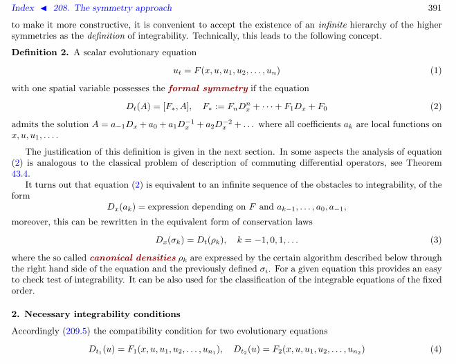
Index J 208. The symmetry approach 391

to make it more constructive, it is convenient to accept the existence of an infinite hierarchy of the highersymmetries as the definition of integrability. Technically, this leads to the following concept.

Definition 2. A scalar evolutionary equation

ut = F (x, u, u1, u2, . . . , un) (1)

with one spatial variable possesses the formal symmetry if the equation

Dt(A) = [F∗, A], F∗ := FnDnx + · · ·+ F1Dx + F0 (2)

admits the solution A = a−1Dx + a0 + a1D−1x + a2D

−2x + . . . where all coefficients ak are local functions on

x, u, u1, . . . .

The justification of this definition is given in the next section. In some aspects the analysis of equation(2) is analogous to the classical problem of description of commuting differential operators, see Theorem43.4.

It turns out that equation (2) is equivalent to an infinite sequence of the obstacles to integrability, of theform

Dx(ak) = expression depending on F and ak−1, . . . , a0, a−1,

moreover, this can be rewritten in the equivalent form of conservation laws

Dx(σk) = Dt(ρk), k = −1, 0, 1, . . . (3)

where the so called canonical densities ρk are expressed by the certain algorithm described below throughthe right hand side of the equation and the previously defined σi. For a given equation this provides an easyto check test of integrability. It can be also used for the classification of the integrable equations of the fixedorder.

2. Necessary integrability conditions

Accordingly (209.5) the compatibility condition for two evolutionary equations

Dt1(u) = F1(x, u, u1, u2, . . . , un1), Dt2(u) = F2(x, u, u1, u2, . . . , un2

) (4)

Index J 208. The symmetry approach 392

can be rewritten in the form

[Dt1 − (F1)∗, Dt2 − (F2)∗] = 0 ⇔ Dt1((F2)∗)−Dt2((F1)∗) = [(F1)∗, (F2)∗]. (5)

Definition 3. Integrable hierarchy, (IH) is the series

A = a0D + a1 + a2D−1 + a3D

−2 + . . . , aj ∈ U (6)

together with a set of functions

H(A) = Fn ∈ U : Dn(A) = Dn(a0)D +Dn(a1) +Dn(a2)D−1 + · · · = [Fn,∗, A] (7)

where Dn(u) := Fn.

We call A the basic operator of the hierarchy and consider as identical one another basic operatorA = α(D)A obtained by multiplication on the series

α0D + α1 + α2D−1 + α3D

−2 + . . . , αj ∈ C

with constant coefficients.Clearly, for F1, F2 ∈ H(A) we can define F3 ∈ U using following general formulae:

F3 = D1(F2)−D2(F1) ⇔ F3 = F2,∗(F1)− F1,∗(F2) := F1, F2. (8)

ThenD3 = [D1, D2], D3 − (F3)∗ = [D1 − (F1)∗, D2 − (F2)∗]

and the Jacobi identity implies that F3 ∈ H(A). Thus H(A) ⊂ U is a Lie algebra with multiplication (8).One can see f1 = u1 belongs to any hierarchy since f1,∗ = D and for any formal series (6) we have

[D,A] = D(a0)D +D(a1) +D(a2)D−1 + · · · = D(A).

On the other hand, the compatibility condition (7) became extremely restrictive in the case of higher orderm ≥ 2 of the function F ∈ U . Most known IH bear the names of the corresponding equations ut = F ∈ H

Index J 208. The symmetry approach 393

of the minimal order n0. Here we have an analogy with the DO B of the minimal order m > 1 in thenontrivial centraliser B ∈ C(A) (see end of the previous section). Moreover, in virtue of Svinolupov theorem,this minimal order for “nontrivial” IH satisfies the condition n0 > 2. Well known integrable hierarchiescorrespond to the following list of third order equations.

KdV type equations

ut = u3 + P (u)u1, P ′′′ = 0, (9)

ut = u3 −1

2u3

1 + (αe2u + βe−2u)u1, (10)

ut = u3 −3

2

u22

u1+r(u)

u1, r(5) = 0. (11)

For a comparison each with others distinct integrable hierarchies the following definition is useful.

Definition 4. The integrable hierarchy H(A2) is called reducible to H(A1) if a differential operator Bexists with coefficients from U such that

A2 = B A1 B−1.

Example 5 (Burgers-hierarchy). One can easily verify that At = [f∗, A] in the case

ut = uxx + 2uux = f, A = D + u+ u1D−1.

Thus, a basic operator for the Burgers equation

A = D + u+ u1D−1 = D(D + u)D−1,

is related to A = D + u by the conjugation. One can verify that evolution equation

Dτ (u) = Dx(u2 + 3uux + u3)

belongs to the Burgers hierarchy H(A) as well.

Index J 208. The symmetry approach 394

It is not difficult to prove that

At = [F∗, A] ⇔ (Aj)t = [F∗, Aj ], j = −1, 1, 2, . . . .

Therefore, the order of the formal series (6) in the definition of the integrable hierarchy may be arbitrary.Next, let F ∈ U and ordF∗ = m > 1, i.e.

F∗ = f0Dm + f1D

m−1 + · · ·+ fm.

Put in the compatibility condition At = [f∗, A]

A = a0Dm + a1D

m−1 + a2Dm−2 + . . .

with undeterminate coefficients. Then collecting the coefficients by Dk, k = 2m−1, 2m−2, . . . ,m+ 1 showsthat in the Definition 3 one may set, without loss of generality,

A = F∗ + g0D + g1 + g2D−1 + . . . . (12)

In other words first m − 1 coefficients of the series (6) are related with the coefficients of the m-th orderdifferential operator F∗ if F ∈ H(A).

Example 6 (Linear equations). Hierarchies H(A) with differential operators A correspond to linear equations(1). In the second order case with A = D2 + a we obtain Fj = Aj(u) ∈ H and, particularly,

ut = uxx + a(x)u = F ⇔ At = [F∗, A].

For “special potentials” a when there is odd order DO B ∈ C(A) there arise additional terms Fk = Bk(u) ofthis hierarchy.

Example 7 (KdV-hierarchy). In KdV case one can find the recursion operator A (cf (12)):

ut = uxxx + 6uux := F, F∗ = D3 + 6uD + 6ux, A = D2 + 4u+ 2uxD−1 (13)

The check of compatibility condition At = [F∗, A] is easy:

4F + 2D(F )D−1 = [D3 + 6Du,D2 + 4u+ 2u1D−1].

Index J 208. The symmetry approach 395

The intermediate corollary of the formula (13) and Theorem 10 below is the sequence of the local con-servation laws of KdV equation i.e. differential corollaries of the equation (13) of the divergent form:

Dt(ρ) = Dx(σ), ρ, σ ∈ U .

The densities ρ of these conservation laws are common for all members of the hierarchy and are defined asfollows.

Definition 8. For an integrable hierarchy H(A) with defining operator (6) the canonical series of thedensities ρj ∈ U , j = −1, 1, 2, . . . is as follows

ρj = resAj , j = −1, 1, 2, . . . . (14)

Lemma 9. For all m,n ∈ Zres[aDm, bDn] = Dxαm,n

where αm,n is a differential polynomial on a and b.

Proof. The residue vanish if the powers m,n obey the condition mn ≥ 0. For instance in the case n = 0the commutator aDmb − baDm is a DO if m ≥ 0 and PDO of order m − 1 ≤ −2 if m < 0. Obviously thecoefficient by D−1 is zero in both cases. Obviously as well that the residue vanish if m+ n < 0.

Let now m,n have different signs and m+ n = k ≥ 0. Then

res[aDm, bDn] =

(m

k + 1

)(aDk+1(b) + (−1)kDk+1(a)b)

sincem+ n = k ⇒ m(m− 1) · · · (m− k) = ±n(n− 1) · · · (n− k).

Standard “integration by parts” completes the proof. Particularly for k = 0, 1 we have, respectively

aD(b) +D(a)b = D(ab) aD2(b)−D2(a)b = D(aD(b)−D(a)b).

Theorem 10. Let A be the basic operator (6) of the integrable hierarchy H(A). Then, for any F ∈ H(A)the equation ut = F possess a series of conservation laws with the canonical densities (14).

Index J 208. The symmetry approach 396

Proof. Using Lemma 9 we find

At = [f∗, A] ⇒ Ajt = [f∗, Aj ] ⇒ Dt(resAj) = res[f∗, A

j ] ∈ ImD.

In the case ρ0 we have

At = [f∗, A] ⇒ AtA−1 = F∗ −AF∗A−1 = [A−1, AF∗].

Therefore

res(AtA−1) = res(a0,tD + a1,t + . . . )(b0D

−1 + b1D−2 + . . . ) =

(a1

a0

)t

∈ ImD.

We used here the equalities a0b0 = 1, a0b1 + a1b0 = 0.

Particularly, this theorem imply that the canonical density ρ−1 = a−10 generates local conservation law

for any n-th order equation ut = Fn ∈ H(A). It follows from formulae (12) that an0 = ∂Fn/∂un and thisgives rise to the first integrability condition

Dt

(∂Fn∂un

)− 1n

∈ ImD (15)

which is necessary condition for ut = Fn to belong to some integrable hierarchy H(A).We should recall that two conservation laws with the densities ρ1 and ρ2 are considered equivalent if

ρ2 ∼ ρ2 and ρ ∼ 0 meansρ = Dx(σ) ⇒ Dt(ρ) = Dx(Dtσ).

This conservation law is considered trivial.Integrability conditions analogous (15) play important role in the classification of IH and equation (12)

allows to rewrite several first canonical densities explicitly.

Example 11. For an evolutionary PDE (1) of the form

ut = un + F (u, u1, . . . , uk), k < n, n ≥ 2 (16)

Fk = ∂ukF is a density of a local conservation law. For equations of the third order

ut = u3 + F (x, u, u1), ρ1 = F1, ρ2 = F0, ρ3 = σ1 (17)

Index J 208. The symmetry approach 397

References

[1] V.V. Sokolov, A.B. Shabat. Classification of integrable evolution equations. Sov. Sci. Rev. C / Math. Phys. Rev.4 (1984) 221–280.

[2] A.V. Mikhailov, A.B. Shabat, R.I. Yamilov. The symmetry approach to classification of nonlinear equations.Complete lists of integrable systems. Russ. Math. Surveys 42:4 (1987) 1–63.

[3] A.V. Mikhailov, A.B. Shabat, V.V. Sokolov. The symmetry approach to classification of integrable equations.In: What is Integrability? (V.E. Zakharov ed). Springer-Verlag, 1991, pp. 115–184.

[4] V.E. Adler, A.B. Shabat, R.I. Yamilov. Symmetry approach to the integrability problem. Theor. Math. Phys.125:3 (2000) 1603–1661.

[5] N.H. Ibragimov, A.B. Shabat. Evolutionary equations with nontrivial Lie–Backlund group. Funct. Anal. Appl.14:1 (1980) 25–36.

[6] A.S. Fokas. A symmetry approach to exactly solvable evolution equations. J. Math. Phys. 21:6 (1980) 1318–1325.

[7] A.S. Fokas. Symmetries and integrability. SIAM J. Math. Anal. 77 (1987) 253–299.

[8] I.M. Bakirov. On the symmetries of some system of evolution equations. Preprint Inst. of Math., Ufa, 1991. (inRussian)

[9] P.H. van der Kamp, J.A. Sanders. On testing integrability. J. Nonl. Math. Phys. 8:4 (2001) 561–574.

Index J 209. Symmetry, higher 398

209 Symmetry, higher

Author: A.B. Shabat, 20.04.2007

Due to the Backlund theorem the groups of transformations depending on the higher order derivativesdo not exist. However, the very natural and rich in content generalization is possible of the infinitesimaldefinition.

In a very general sense, a symmetry of a partial differential (or difference equation) is just anotherequation which is consistent with it. Consider the simplest case of the evolutionary PDEs with one spatialvariable

ut = F (x, u, u1, . . . , un) (1)

where uk stands for k-th order derivative with respect to x. One says that another such equation

uT = G(x, u, u1, . . . , um)

is a generalized or higher symmetry of (1) if the cross derivatives coincide: utT = uTt, or DT (F ) = Dt(G).To make this definition precise one have to formalize the definition of x, t- and T -derivatives. We consider

x, u, u1, . . . as independent dynamical variables (this approach is traditional for the differential algebra,see e.g. [3], where uk are called differential indeterminate). Then the x-derivative is replaced with theoperator of total derivative

Dx = ∂x + u1∂u + · · ·+ uk+1∂uk+ . . . ,

Dx : x→ 1, u→ u1 → · · · → uk → uk+1 → . . . .

Let F denotes the set of locally smooth functions on the finite number of dynamical variable. Any suchfunction can be differentiated with respect to t in virtue of equation (1) accordingly to the chain rule:

Dt(G) = GuF +Gu1Dx(F ) + · · ·+Gum

Dmx (F ).

The result can be conveniently written as

Dt(G) = ∇F (G) = G∗(F )

Index J 209. Symmetry, higher 399

by use of the vector field called evolutionary derivative

∇F := F∂u +Dx(F )∂u1+ · · ·+Dk

x(F )∂uk+ . . . (2)

and the differential operator called Frechet derivative or Gato derivative or linearization operator

G∗ := Gu +Gu1Dx + · · ·+Gum

Dmx , G∗(v) =

( ddεG[u+ εv]

)∣∣∣ε=0

. (3)

Definition 1. An evolutionary PDE uT = G(x, u, u1, . . . , um) is called the symmetry of (1) if the cor-responding evolutionary derivatives commute: [∇F ,∇G] = 0. The set of all G satisfying this equation isdenoted Sym(F ).

In addition to the commutator of vector fields, we will use the brackets for denoting of the commutatorof differential operators, and also for the operation

[F,G] := ∇F (G)−∇G(F ) = G∗(F )− F∗(G), F,G ∈ F . (4)

This does not lead to any misunderstanding, since the use of notation is clear from the type of operands.

Obviously, both ∇F and F∗ are linear in F . The other important properties of the introduced operationsare listed below.

Statement 2. The identities hold:

1) [Dx,∇F ] = 0;

2) [∇F ,∇G] = ∇[F,G];

3) [F, [G,H]] + [G, [H,F ]] + [H, [F,G]] = 0;

4) (FG)∗ = FG∗ +GF∗;

5) (Dx(F ))∗ = DxF∗;

6) [∇F − F∗,∇G −G∗] = ∇[F,G] − [F,G]∗.

Index J 209. Symmetry, higher 400

Proof. 1,2) It is sufficient to apply the commutator to the dynamical variables x, u = u0, u1, . . . We have:

1) [Dx,∇F ](x) = 0, [Dx,∇F ](uk) = Dx(Dkx(F ))−∇F (uk+1) = 0 ⇒ [Dx,∇F ] = 0;

2) [∇F ,∇G](x) = 0, [∇F ,∇G](uk) = ∇F (Dkx(G))−∇G(Dk

x(F ))

1)= Dk

x(∇F (G)−∇G(F )) = Dkx([F,G]) ⇒ [∇F ,∇G] = ∇[F,G].

The identity 3) follows from 2) and the Jacobi identity for the vector fields. The identity 4) is obvious, 5)requires some calculations:

(Dx(F ))∗ =(∑

k

Fukuk+1

)∗

=∑k

FukDk+1x +

∑j,k

uk+1Fuk,ujDjx = Dx

∑k

FukDkx = DxF∗.

In order to prove 6), we first prove the relation (∇F (G))∗ = [∇F , G∗] +G∗F∗:

(∇F (G))∗ =(∑

k

GukDkx(F )

)∗

=∑k

(Guk

DkxF∗ +Dk

x(F )∑j

Guk,ujDjx

)= G∗F∗ +

∑j,k

Dkx(F )Guk,uj

Djx = G∗F∗ +

∑j

∇F (Guj)Dj

x = G∗F∗ + [∇F , G∗].

Now, 6) follows from here and 2):

[∇F − F∗,∇G −G∗] = [∇F ,∇G]− [∇F , G∗]−G∗F∗ + [∇G, F∗] + F∗G∗

= ∇[F,G] − (∇F (G))∗ + (∇G(F ))∗ = ∇[F,G] + [F,G]∗.

In particular, this statement implies that the following definitions of symmetry are equivalent:

[∇F ,∇G] = 0 ⇔ [F,G] = 0 ⇔ (∇F − F∗)(G) = 0 ⇔ [∇F − F∗,∇G −G∗] = 0. (5)

The latter formula is of particular importance for the definition of the necessary integrability conditions (seesymmetry approach).

Index J 209. Symmetry, higher 401

Moreover, the Jacobi identity 3) implies that the space F equipped with the operation [, ] is a Lie algebraand the symmetries set Sym(F ) is its Lie subalgebra. The integrable equations can be defined as thosewith an infinite-dimensional Lie algebra of symmetries. The structure of this Lie algebra can be different. Ifthe equation is linearizable then it contains an infinite-dimensional Lie subalgebra of classical symmetries.For the KdV-type equations it is typical that classical symmetries form a finite-dimensional noncommutativeLie subalgebra while the higher symmetries form an infinite-dimensional commutative Lie subalgebra (called“hierarchy”).

References

[1] V.V. Sokolov. On the symmetries of evolution equations. Russ. Math. Surveys 43:5 (1988) 165–204.

[2] P.J. Olver. Applications of Lie groups to differential equations, 2nd ed., Graduate Texts in Math. 107, NewYork: Springer-Verlag, 1993.

[3] J.F. Ritt. Differential Algebra. AMS Colloquim Publ. 33, 1948.

Index J 210. Thomas equation hDD 402

210 Thomas equation

uxt = aut + bux + cuxut

References

[1] R.R. Rosales. Exact solutions of a certain nonlinear wave equation. J. Math. Phys. 45 (1966) 235–265.

Index J 211. Toda lattice eD∆ 403

211 Toda lattice

qn,xx = eqn+1−qn − eqn−qn−1

ã The higher symmetries

qn,t2 = q2n,x + eqn+1−qn + eqn−qn−1 , qn,t3 = q3

n,x + (qn+1 + 2qn)xeqn+1−qn + (2qn + qn−1)xe

qn−qn−1 , . . .

can be rewritten as the NLS hierarchy for the variables u = eqn , v = e−qn−1 :

ut2 = uxx + 2u2v, −vt2 = vxx + 2v2u; ut3 = uxxx + 6uvux, vt3 = vxxx + 6uvvx; . . .

ã Hamiltonian structure (pn = qn,x):

pn, qn = 1, H =∑(1

2p2n + eqn+1−qn

).

ã Zero curvature representation:

Ln =

(qn,x + 2λ eqn

−e−qn 0

), Un =

(−λ −eqn

e−qn−1 λ

)

References

[1] M. Toda. Vibration of a chain with nonlinear interaction. J. Phys. Soc. Japan 20 (1967) 431–436.

[2] M. Toda. Theory of nonlinear lattices. Solid-State Sci. 20, Springer-Verlag, 1981.

Index J 212. Toda lattice, two-dimensional eDD∆ 404

212 Toda lattice, two-dimensional

qn,xy = eqn+1−qn − eqn−qn−1

ã Introduced in [1]

ã In slightly different form, 2D Toda lattice describes the sequence of Laplace invariants.ã Infinite Toda lattice admits a number of reductions to finite exponential systems. The most importantexamples are related to semisimple Lie algebras, see e.g. [2].

References

[1] A.V. Mikhailov. Integrability of a two-dimensional generalisation of the Toda chain. Sov. Phys. JETP Lett 30(1979) 414–418.

[2] A.N. Leznov, M.V. Savel’ev. Group methods for integrating of nonlinear dynamical systems. Moscow: Nauka,1985.

Index J 213. Toda lattice, relativistic eD∆ 405

213 Toda lattice, relativistic

qn,xx = g2qx

(qn−1,x

eqn−1−qn

1 + g2eqn−1−qn− qn+1,x

eqn−qn+1

1 + g2eqn−qn+1

)

References

[1] S.N.M. Ruijsenaars. Relativistic Toda system. Preprint Stichting Centre for Math. and Comp. Sciences, Ams-terdam, 1986.

[2] S.N.M. Ruijsenaars. Relativistic Toda systems Commun. Math. Phys. 133:2 (1990) 217–247.

Index J 214. Tops. Pairs of commuting Hamiltonians quadratic in momenta 406

214 Tops. Pairs of commuting Hamiltonians quadratic in momenta

Author: V.G. Marikhin, 27.08.2007

1. Diagonalization of quadratic part2. Universal solution of Hamilton–Jacobi equation3. Examples

In this article we study the pairs of Hamiltonians of the form

H = ap21 + 2bp1p2 + cp2

2 + dp1 + ep2 + f, K = Ap21 + 2Bp1p2 + Cp2

2 +Dp1 + Ep2 + F (1)

commuting with respect to the standard Poisson bracket pα, qβ = δαβ . The coefficients of the Hamiltoniansare assumed to be locally analytical functions of q1, q2. This problem was considered in papers [1, 2, 3, 4,5, 6, 7]. Here we present some new many-parametrical families of such pairs and the universal method ofconstructing the full solution of Hamilton–Jacobi equation in terms of integrals on some algebraic curve. Inseveral examples this curve is a non-hyperelliptic covering over an elliptic curve.

1. Diagonalization of quadratic part

It is possible to introduce new coordinates s1, s2 such that quadratic parts of H,K became diagonal. Thecondition H,K = 0 is essential for existence of this transformation. Let s1, s2 be roots of equation

Φ(s, q1, q2) = (B − bs)2 − (A− as)(C − cs) = 0

and Φi = Φ(si, q1, q2), then the canonical transformation

(q1, q2, p1, p2)→ (s1, s2, P1, P2) : p1 = −

(Φ1q1

Φ1s1

P1 +Φ2q1

Φ2s2

P2

), p2 = −

(Φ1q2

Φ1s1

P1 +Φ2q2

Φ2s2

P2

)brings the pair (1) to the form

H =S1(s1)

s1 − s2P 2

1 −S2(s2)

s1 − s2P 2

2 + dP1 + eP2 + f , K =s2S1(s1)

s1 − s2P 2

1 −s1S2(s2)

s1 − s2P 2

2 + DP1 + EP2 + F ,

Index J 214. Tops. Pairs of commuting Hamiltonians quadratic in momenta 407

where

Si(si) =1

(Φiqi)2

((asi −A)(Φiq1)2 + 2(bsi −B)Φiq1Φiq2 + (csi − C)(Φiq2)2).

Theorem 1. Any pair of commuting Hamiltonians (1) can be brought by canonic transformation

P1 = P1 +∂F (s1, s2)

∂s1, P2 = P2 +

∂F (s1, s2)

∂s2

to the pair of the form

H =U1 − U2

s1 − s2, K =

s2U1 − s1U2

s1 − s2(2)

where

U1 = S1(s1)P 21 +

√S1(s1)S2(s2)Zs1

(s1 − s2)P2 −

S1(s1)Z2s1

4(s1 − s2)2+ V1(s1, s2),

U2 = S2(s2)P 22 −

√S1(s1)S2(s2)Zs2

(s1 − s2)P1 −

S2(s2)Z2s2

4(s2 − s1)2+ V2(s1, s2),

(3)

V1 =1

2

√S1(s1)∂s1

(√S1(s1)

Z2s1

s1 − s2

)+ f1(s1),

V2 =1

2

√S2(s2)∂s2

(√S2(s2)

Z2s2

s2 − s1

)+ f2(s2)

(4)

for some functions Z(s1, s2), Si(si) and fi(si). The Poisson bracket H,K equals to zero if and only if thefollowing conditions are fulfilled:

Zs1,s2 =Zs1 − Zs22(s2 − s1)

, (5)

(Zs1∂s2 − Zs2∂s1)

(V1 − V2

s1 − s2

)= 0. (6)

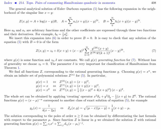
Index J 214. Tops. Pairs of commuting Hamiltonians quadratic in momenta 408

The general analytical solution of Euler–Darboux equation (5) has the following expansion in the neigh-borhood of the singular line x = y:

Z(x, y) = A+ log(x− y)B, A =

∞∑0

ai(x+ y)(x− y)2i, B =

∞∑0

bi(x+ y)(x− y)2i.

Here a0 and a1 are arbitrary functions and the other coefficients are expressed through these two functionsand their derivatives. For example, b0 = 1

2a′′0 .

We insert this expansion into (6) in order to prove B = 0. It is easy to check that any solution of theequation (5) with B = 0 is of the form

Z(x, y) = z0 + δ(x+ y) + (x− y)2∞∑k=0

g(2k)(x+ y)

2(2k)k!(k + 1)!(x− y)2k, (7)

where g(x) is some function and z0, δ are constants. We call g(x) generating function for (7). Without lossof generality we choose z0 = 0. The parameter δ is very important for classification of Hamiltonians fromTheorem 1.

We find all functions Z, corresponding to the rational generating functions g. Choosing g(x) = xn, weobtain an infinite set of polynomial solutions Z(n) for (5). In particular,

g(x) = 1 ⇔ Z(0)(x, y) = (x− y)2,g(x) = x ⇔ Z(1)(x, y) = (x+ y)(x− y)2,g(x) = x2 ⇔ Z(2)(x, y) = 1

4

((x− y)2 + 4(x+ y)2

)(x− y)2.

The whole set can be obtained by applying ‘creating’ operator x2∂x + y2∂y − 12 (x+ y) to Z0. The rational

functions g(x) = (x− µ)−n correspond to another class of exact solution of equation (5), for example

gµ(x) =1

4(x− 2µ)⇔ Zµ(x, y) =

√(µ− x)(µ− y) +

1

2(x+ y)− µ.

The solution corresponding to the poles of order n ≥ 2 can be obtained by differentiating the last formulawith respect to the parameter µ. Since function Z is linear in g we obtained the solution Z with rationalgenerating function g(x) =

∑i cix

i +∑i,j dij(x− µi)−j .

Index J 214. Tops. Pairs of commuting Hamiltonians quadratic in momenta 409

Conjecture 2. For all Hamiltonians (2)–(6) the generating function g is rational of the form g(x) = P (x)S(x) ,

where P and S are polynomials with degP < 5, degS < 6.

In papers [5, 6] the following solution of the system (5), (6) has been considered:

Z(x, y) = x+ y, S1(x) = S2(x) =

6∑i=0

cixi, f1(x) = f2(x) = −3

4c6x

4 − 1

2c5x

3 +

2∑i=0

kixi

where ci, ki are constants. It should be noted that Clebsch top and so(4)-Schottky–Manakov top [8, 9, 10]are the particular cases of this model [6]. The full solution of Hamilton–Jacobi equation of this model wasobtained in [6] by means of some kind of separation of variables on a non-hyperelliptic curve of genus 4.

2. Universal solution of Hamilton–Jacobi equation

Let H and K be of the form (2)–(4) and let p1 = F1(x, y), p2 = F2(x, y) be solution of the system H = e1,K = e2 where ei are constants. Here and below we denote for short x = s1, y = s2. Accordingly to Jacobilemma, if H, K = 0 then F1,y = F2,x. To find the action S(x, y, e1, e2) it is sufficient to solve the system

Sx = F1, Sy = F2.

We rewrite the system H = e1, K = e2 in the form

p21 + ap2 + b = 0, p2

2 +Ap1 +B = 0, (8)

where

a =Zxx− y

√S2(y)

S1(x), A = − Zy

x− y

√S1(x)

S2(y), (9)

b = − Z2x

4(x− y)2+V1 − e1x+ e2

S1(x), B = −

Z2y

4(x− y)2+V2 − e1y + e2

S2(y). (10)

Index J 214. Tops. Pairs of commuting Hamiltonians quadratic in momenta 410

It easy to prove the following identities (the last one is obtained by use of (5), (6)):

2by +Aax + 2aAx = 0, 2Aay + aAy + 2Bx = 0, (11)

Abx − aBy + 2Axb− 2ayB = 0. (12)

Using the standard technique of Lagrange resolvents, we rewrite the system (8) in the form

uv =1

4aA, Au3 +

4b

au2v − 4B

Auv2 − av3 = 0, (13)

which is equivalent to a cubic equation on u2. Let (uk, vk), k = 1, 2, 3 be solutions of (13) then

u21 + u2

2 + u23 = −b, v2

1 + v22 + v2

3 = −B, 8u1u2u3 = −a2A, 8v1v2v3 = −A2a

and the formulasp1 = u1 + u2 + u3, p2 = v1 + v2 + v3;p1 = u3 − u1 − u2, p2 = v3 − v1 − v2;p1 = u2 − u1 − u3, p2 = v2 − v1 − v3;p1 = u1 − u2 − u3, p2 = v1 − v2 − v3

define four solutions of (8). Consider first of them.

Lemma 3. The equations ui,y = vi,x hold for i = 1, 2, 3.

Proof. Differentiating equations (13) with respect to x and y we find uy and vx as functions on u and v.Then expressing v through u we obtain that uy = vx is equivalent to identities (11), (12).

The above Lemma means that variables u1, u2, u3 are “particular” separation variables. Indeed, theaction takes the form S = S1 +S2 + S3 where functions Si are defined from the system

Si,x = ui, Si,y = vi.

Let

u =Zx

2(x− y)

√y − ξx− ξ

, v = − Zy2(x− y)

√x− ξy − ξ

.

Index J 214. Tops. Pairs of commuting Hamiltonians quadratic in momenta 411

It easy to see that the pair (u, v) is a solution of (13) for all ξ. If Z is a solution of (5) then uy = vx. Usingthis fact we introduce the function σ(x, y, ξ) such that σx = u, σy = v. In the case of a rational functiong the corresponding function Z is expressed through quadratic radicals and the function σ can be foundexplicitly.

After multiplication of second equation (13) by expression

−2

√S1(x)

√S2(y)

√x− ξ

√y − ξ (x− y)

ZxZy

it takes the form

Ψ(x, y, ξ) = −e2 + e1ξ +y − ξx− y

(V1 −

S1(x)Z2x

4(x− ξ)(x− y)

)− x− ξx− y

(V2 +

S2(y)Z2y

4(y − ξ)(x− y)

)= 0.

Statement 4. Let the conditions (5), (6) hold. Then the function Ψ(x, y, ξ) depends on the variables Y = σξand ξ only: Ψ(x, y, ξ) = φ(ξ, Y ).

Proof. Consider Jacobian J = ΨxYy − ΨyYx. We change Yy, Yx to vξ, uξ respectively, then Jacobian Jvanishes identically in virtue of (5), (6). The function φ can be found by setting y = x.

Equation φ(ξ, Y ) = 0 defines a curve, and differentials of this curve define the function of action S. Letξk(x, y), k = 1, 2, 3 be the roots of the cubic equation Ψ(x, y, ξ) = 0.

Theorem 5. Function of action S is of the form

S(x, y) =

3∑k=1

(σ(x, y, ξk)−

∫ ξk

Y (ξ)dξ), (14)

where Y (ξ) is algebraic function defined by equation φ(ξ, Y ) = 0.

Proof. We obtain

Sx(x, y) =

3∑k=1

σx(x, y, ξk) +

3∑k=1

(σξ(x, y, ξk)− Y (ξk))ξk,x =

3∑k=1

uk = p1.

Analogously, Sy(x, y) = p2.

Index J 214. Tops. Pairs of commuting Hamiltonians quadratic in momenta 412

3. Examples

Here we list all known at the moment pairs of Hamiltonians (2)–(6).

Class 1. For models of this class

S1 = S2 = S, f1 = f2 = f. (15)

Theorem 6. Let

g =G

S, G = G− δ

10S′, f = −4G2

S− 4δ

3G′ − δ2

12S′′,

where S(x) = s5x5 + s4x

4 + s3x3 + s2x

2 + s1x+ s0, G(x) = g3x3 + g2x

2 + g1x+ g0 and si, gi, δ are constants.Then functions S, f and function Z corresponding to the generating function g (see Section 214) satisfy thesystems (5), (6).

Remark 7. The parameter δ in Theorem 6 coincides with parameter in (7). In the case δ = 0 this Theoremdescribes all pairs of Hamiltonians (2)–(6), (15).

Consider a general case

S(x) = s5(x− µ1)(x− µ2)(x− µ3)(x− µ4)(x− µ5),

where s5 6= 0 and all zeroes µi are distinct. Then the function Z is of the form

Z(x, y) =

5∑i=1

νi√

(µi − x)(µi − y), nui = const . (16)

Coefficients gi and δ are expressed through constants νi from (7). For example, 2δ = −∑νi. Function f is

defined by

f(x) = − 1

16

5∑i=1

ν2i

S′(µi)

x− µi+ k1x+ k0,

Index J 214. Tops. Pairs of commuting Hamiltonians quadratic in momenta 413

with constant k1, k0.Calculation for a function (16) gives

σ(x, y, ξ) = −1

2

5∑i=1

νi log

√x− ξ

√y − µi +

√y − ξ

√x− µi√

x− y√µi − ξ

, (17)

Y =1

4

N∑i=1

νi

√(x− µi)(y − µi)

(ξ − µi)√

(x− ξ)(y − ξ).

Algebraic curve is hyperelliptic of genus 2: φ(Y, ξ) = S(ξ)Y 2 + f(ξ)− ξe1 + e2 = 0.Steklov top on so(4) [11] is a particular case of Theorem 6.

Class 2. Functions Z for models of this class are the special cases of the functions Z of Class 1. But thisClass contains much more parameters than in Theorem 6.

These functions Z can be defined as solutions of system

Zxy =Zx − Zy2(y − x)

=1

3U(Z)ZxZy, (18)

where U are some functions of one variable.

Remark 8. It easy to see that this class of solutions of Euler–Darboux equation Zxy =Zx−Zy

2(y−x) coincide with

class of solutions of the form

Z = F

(h(x)− h(y)

x− y

),

where U = F ′′/F ′2.

Lemma 9. The system (18) is compatible if and only if

U =3B′

2B, B(Z) = b2Z

2 + b1Z + b0, bi = const .

Index J 214. Tops. Pairs of commuting Hamiltonians quadratic in momenta 414

Three cases are possible:

degB = 2 : Z =√

(x− µ1)(y − µ1) +√

(x− µ2)(y − µ2), b2 = 1, b1 = 0, b0 = −(µ1 − µ2)2, (19)

degB = 1 : Z =√x y +

1

2(x+ y), b1 = 1, b2 = b0 = 0, (20)

degB = 0 : Z = x+ y. (21)

Case degB = 2. Consider function Z of the form (19). Then

S(x) = (x− µ1)(x− µ2)P (x) + (x− µ1)3/2(x− µ2)3/2Q(x), degP ≤ 3, degQ ≤ 2,

f(x) = f0 + f1x+ k2(x− µ1)1/2(x− µ2)1/2 +(µ2 − µ1)

16

( P (µ1)

x− µ1− P (µ2)

x− µ2

)+

(µ2 − µ1)

32(x− µ1)1/2(x− µ2)1/2

(Q(µ1)

x− µ1− Q(µ2)

x− µ2

).

In the case Q = 0, k2 = 0 these formulas coincide with the corresponding formulas of Class 1. The functionsσ, Y are defined by the same formula (17) as for Class 1:

σ(x, y, ξ) = −1

2

2∑i=1

log

√x− ξ

√y − µi +

√y − ξ

√x− µi√

x− y√µi − ξ

, Y =1

4

2∑i=1

√(x− µi)(y − µi)

(ξ − µi)√

(x− ξ)(y − ξ).

Algebraic curve in this case is of the form

(SR(ξ) + ηSI(ξ))Y2 − kR(ξ)− ηkI(ξ) = 0 (22)

where

SR(x) = (x− µ1)(x− µ2)P (x), SI(x) = (x− µ1)(x− µ2)Q(x), (23)

kR(x) = −e2 + e1x− f0 − f1x−(µ2 − µ1)

16

( P (µ1)

x− µ1− P (µ2)

x− µ2

), (24)

Index J 214. Tops. Pairs of commuting Hamiltonians quadratic in momenta 415

kI(x) = k2 −1

32(µ1 − µ2)2 − 1

16(µ1 − µ2)

(Q(µ1)

x− µ1− Q(µ2)

x− µ2

), (25)

1

η=

1√ξ − µ1

√ξ − µ2

√1− (µ1 − µ2)2

16(ξ − µ1)2(ξ − µ2)2Y 2. (26)

Expressing Y as a function of (ξ, η) and substituting to (22) we obtain 10-parameter cubic in (ξ, η) variables.So, in general the curve φ(Y, ξ) = 0 is a covering over an elliptic curve. We obtain

η =ξ − µ1

√x−µ1√x−µ2

+√y−µ1√y−µ2

+ξ − µ2

√x−µ2√x−µ1

+√y−µ2√y−µ1

,

therefore points (ξ1, η1), (ξ2, η2), (ξ3, η3) lie on a straight line.

Case degB = 1. For the function Z of the form (20) we have

S(x) = xP (x) + x3/2Q(x), degP ≤ 3, degQ ≤ 2,

f(x) = − 1

16xP (x)− 1

32√xQ(x) + f1x+ fq

√x+ f0, Y =

ξ +√x√y

4ξ√x− ξ

√y − ξ

.

The curve in this case can be written in the form (22) where

SR(x) = xP (x), SI(x) = xQ(x),

kR(x) = −e2 + e1x− f0 − f1x+1

16xP (x), kI(x) =

1

16xQ(x)− fq, η =

4Y ξ3/2√16Y 2ξ2 − 1

.

In (ξ, η) variables it also has the form of arbitrary cubic. Formula η =ξ+√xy√

x+√y

proves that points (ξ1, η1), (ξ2, η2), (ξ3, η3)

are collinear.

Case degB = 0. For the function Z given by (21) we have

S(x) = s6x6 + s5x

5 + s4x4 + s3x

3 + s2x2 + s1x+ s0,

Index J 214. Tops. Pairs of commuting Hamiltonians quadratic in momenta 416

f(x) = − 1

40S′′(x)− 1

32√xQ(x) + f2x

2 + f1x+ f0, Y =1

2√x− ξ

√y − ξ

.

The algebraic curve is

S(ξ)Y 6 − F (ξ)Y 4 −(1

8F ′′(ξ) +

7

1920SIV (ξ)− k2

2

)Y 2 − s6

64= 0, F (ξ) = −e2 + e1ξ − f(ξ).

It is an arbitrary cubic in the variables (ξ, η), where η = ξ2 − 1/(4Y 2). Since η = ξ(x + y)− xy the points(ξ1, η1), (ξ2, η2), (ξ3, η3) are collinear.

Class 3. We will say that Hamiltonian (2)–(6) is non-symmetrical if S1(x) 6= S2(x) or f1(x) 6= f2(x).

Theorem 10 ([7]). In non-symmetrical case the functions Z, Si, fi are solutions of (5), (6) if and only if

δ = 0, g =1

H, S1,2 = WH ±MH3/2, f1,2 = −4W

H∓ 2MH−1/2 ± aH1/2,

where g is the generating function for Z and

W (x) = w3x3 + w2x

2 + w1x+ w0, H(x) = h2x2 + h1x+ h0, M(x) = m2x

2 +m1x+m0

with constant wi, hi,mi, a.

Consider the general case H(x) = (x − µ1)(x − µ2). The algebraic curve Ψ(ξ, Y ) = 0 in this case is ofthe form

−e2+e1ξ−RW (ξ)

2(ξ − µ1)(ξ − µ2)(µ2 − µ1)+4M(ξ)

√2Y

√ξ − µ1

√ξ − µ2

(µ2 − µ1)3/2

√R+8b

√2Y

(ξ − µ1)3/2(ξ − µ2)3/2

√R√µ2 − µ1

= 0

where

Y =

√(x− µ1)(y − µ1)

(ξ − µ1)√

(x− ξ)(y − ξ)−

√(x− µ2)(y − µ2)

(ξ − µ2)√

(x− ξ)(y − ξ), R = 16(ξ − µ1)2(ξ − µ2)2Y 2 − (µ1 − µ2)2.

Index J 214. Tops. Pairs of commuting Hamiltonians quadratic in momenta 417

Substituting

Y =(µ1 − µ2)3/2η

4(ξ − µ2)(ξ − µ1)√η2(µ2 − µ1)− 8(ξ − µ1)(ξ − µ2)

into this equation we obtain the cubic in variables (ξ, η) with a full set of ten independent parameters. Iteasy to see that η = a(x, y)ξ + b(x, y) where a, b are some functions.

Summing up, we have seen that in all cases of Classes 2 and 3 the algebraic curve is a non-hyperelliptic cov-ering over an elliptic curve. The dynamics of the points (ξ1, Y1), (ξ2, Y2), (ξ3, Y3) on this curve (see Theorem 5)satisfies the following condition: the projections of these points onto the elliptic base (ξ1, η1), (ξ2, η2), (ξ3, η3)lie on a straight line.

Conjecture 11. Any pair of the Hamiltonians (2)–(6) belongs to one of above three classes.

References

[1] B. Dorizzi, B. Grammaticos, A. Ramani, P. Winternitz. Integrable Hamiltonian systems with velocity dependentpotentials. J. Math. Phys. 26:12 (1985) 3070–3079.

[2] E.V. Ferapontov, A.P. Fordy. Non-homogeneous systems of hydrodynamic type, related to quadratic Hamilto-nians with electromagnetic term. Physica D 108:4 (1997) 350–364.

[3] E.V. Ferapontov, A.P. Fordy. Commuting quadratic Hamiltonians with velocity dependent potentials. Rep.Math. Phys. 44:1,2 (1999) 53–70.

[4] E. McSween, P. Winternitz. Integrable and superintegrable Hamiltonian systems in magnetic fields. J. Math.Phys. 41 (2000) 2957–2967.

[5] H.M. Yehia. Generalized natural mechanical systems of two degrees of freedom with quadratic integrals. J. Phys.A 25:1 (1992) 197–221.

[6] V.G. Marikhin, V.V. Sokolov. Separation of variables on a non-hyperelliptic curve. Reg. and Chaot. Dyn. 10:1(2005) 59–70.

[7] V.G. Marikhin, V.V. Sokolov. On quasi-Stackel Hamiltonians. Russ. Math. Surveys 60:5 (2005) 981–983.

Index J 214. Tops. Pairs of commuting Hamiltonians quadratic in momenta 418

[8] F. Schottky. Uber das analytische Problem der Rotation eines starren Korpers in Raume von vier Dimensionen.Sitzungsberichte der Koniglich preussischen Academie der Wissenschaften zu Berlin XIII (1891) 227–232.

[9] S.V. Manakov. A remark on integration of the Euler equations for n-dimensional rigid body dynamics. Funct.Anal. Appl. 10 (1976) 328–329.

[10] A. Clebsch. Uber die Bewegung eines Korpers in einer Flussigkeit. Math. Annalen 3 (1870) 238–262.

[11] V.A. Stekloff. Sur le mouvement dun corps solide ayant une cavite de forme ellipsoidale remple par un liquideincompressible en sur les variations des latitudes. Ann. de la fac. des Sci. de Toulouse, Ser. 3, v. 1 (1909).

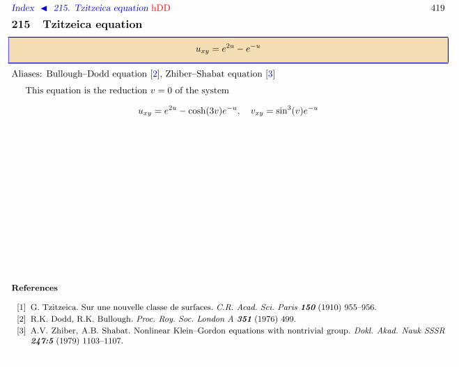
Index J 215. Tzitzeica equation hDD 419

215 Tzitzeica equation

uxy = e2u − e−u

Aliases: Bullough–Dodd equation [2], Zhiber–Shabat equation [3]

This equation is the reduction v = 0 of the system

uxy = e2u − cosh(3v)e−u, vxy = sin3(v)e−u

References

[1] G. Tzitzeica. Sur une nouvelle classe de surfaces. C.R. Acad. Sci. Paris 150 (1910) 955–956.

[2] R.K. Dodd, R.K. Bullough. Proc. Roy. Soc. London A 351 (1976) 499.

[3] A.V. Zhiber, A.B. Shabat. Nonlinear Klein–Gordon equations with nontrivial group. Dokl. Akad. Nauk SSSR247:5 (1979) 1103–1107.

Index J 216. Variational derivative 420

216 Variational derivative

The variational problem is called the problem on finding the extrema of the functional

L[u] =

∫Ω

L[x, uσ]dx, L ∈ R, x ∈ Rm, u ∈ Rn

where the Lagrange function L depends on x and a finite set of derivatives uσ = Dσ(u) = Dσ1x1· · ·Dσm

xm(u1, . . . , un).

The solution of this problem is defined by Euler–Lagrange equation (with appropriate boundary condi-tions)

δL = 0, δ =( δ

δu1, . . . ,

δ

δun

),

δ

δuj=∑σ

(−D)σ∂

∂ujσ=∑σ

(−Dx1)σ1 . . . (−Dxm

)σm∂

∂ujσ.

The operator δ/δuj is called the variational derivative. The term Euler operator and the notationEuj are used as well. The Euler–Lagrange equation is written compactly as Lᵀ

∗(1) = 0 by use of Frechetderivative and the formal conjugation of differential operators.

In the discrete setup the variational derivative is of the form

δ

δuj=∑σ

T−σ∂

∂ujσ=∑σ

T−σ11 . . . T−σm

m

∂

∂ujσ

where Ti is the shift operator xi → xi + 1. The definition in the case of mixed continuous and discreteindependent variables is straightforward as well.

References

[1] P.J. Olver. Applications of Lie groups to differential equations, 2nd ed., Graduate Texts in Math. 107, NewYork: Springer-Verlag, 1993.

Index J 217. Vector field 421

217 Vector field

A vector field on a manifold M is a smooth mapping F : x → TxM , x ∈ M . In a local coordinatesx = (x1, . . . , xn) on M , the vector field is given by an expression of the form

F = f1(x)∂x1 + . . . fn(x)∂xn

where f i are smooth functions on M and ∂xi ∈ TxM is the tangent vector to the i-th coordinate line.The formula F (a) = f1ax1 +. . . fnaxn associates the vector field with the differentiation in the associative

algebra of the smooth functions on M . The converse is true as well, that is any differentiation is definedby a vector field, and its components are just the values of the differentiation on the coordinate functionsxi. The commutator of the differentiations defined as [F,G](a) = F (G(a)) − G(F (a)) corresponds to thecommutator of the vector fields

[F,G] = (F (g1)−G(f1))∂x1 + · · ·+ (F (gn)−G(fn))∂xn

which equips the space of the vector fields with the structure of a Lie algebra.The existence of some additional structures on the manifold allows to distinguish several special Lie

subalgebras of the vector fields. For example, a Hamiltonian vector field XH is defined by a single functionH accordingly to the rule XH(a) = H, a if M is equipped with a Poisson bracket.

ã See also: contact vector field, evolutionary derivative.

References

[1] P.J. Olver. Applications of Lie groups to differential equations, 2nd ed., Graduate Texts in Math. 107, NewYork: Springer-Verlag, 1993.

Index J 218. Vector integrable evolutionary equations 422

218 Vector integrable evolutionary equations

Author: V.V. Sokolov, 08.02.2009

1. Introduction. Examples2. Definitions and notations3. Isotropic equations on the sphere4. Anisotropic equations on the sphere5. Backlund transformations for equations on the sphere6. Divergent equations

1. Introduction. Examples

An example of vector equation is given by two different vector analogs of mKdV equation:

ut = u3 + (u,u)u1, and ut = u3 + (u,u)u1 + (u,u1)u.

Here u denotes a N -dimensional vector and (·, ·) stands for the standard scalar product. It is well knownthat these equation are integrable at any N by inverse scattering method and, consequently, possess infinitesets of symmetries and conservation laws. It is clear that both equations possess SO(N)-symmetry (that is,are invariant with respect to all rotations). Such equations are called isotropic. These examples belong tothe class of isotropic equations of the general form

ut = u3 + f2u2 + f1u1 + f0u (1)

where the coefficients fi are real-valued functions with the argument set of six different scalar products ofthe vectors u,u1 and u2.

A more general class of equations (1) consists of vector anisotropic equations. The example of such anequation is [1]

ut =(u2 +

3

2(u1,u1)u

)x

+3

2(u, Ru)u1, (u,u) = 1 (2)

where R is an arbitrary constant symmetric matrix. If N = 3 then (2) is the symmetry of the famousLandau–Lifshitz equation. Equation (2) is integrable for any N and R. In contrast to the isotropic case, the

Index J 218. Vector integrable evolutionary equations 423

coefficients of anisotropic equations (1) depend on six more arguments defined by means of additional scalarproduct 〈X,Y 〉 = (X,RY ).

2. Definitions and notations

Let us introduce the following notations. In the isotropic case, let F denote the set of locally analyticfunctions on the variables

u[i,j] = (ui,uj), 0 ≤ i ≤ j. (3)

Here (·, ·) is a scalar product in a N -dimensional (or infinite-dimensional) vector space V .In the anisotropic situation, let F denote the set of locally analytic functions on the variables (3) and

additional variablesu[i,j] = 〈ui,uj〉, 0 ≤ i ≤ j (4)

where 〈·, ·〉 is another scalar product in V . The differential order of the variables u[i,j] and u[i,j] is equal j.If a function depends on variables (3) and (4) up to order n then we say that n is order of this function.

We consider the properties of vector equations which do not depend on the nature of the space V and ofthe scalar products. This important assumption is formalized as follows: no constraints exist between thescalar products (3), (4) which will play the role of independent variables.

The results on the formal symmetry obtained in papers [2, 3, 4, 5] can be generalized in the vector caseas follows:

Theorem 1 ([6]). i) If equation (1) possesses an infinite sequence of the symmetries of the form

uτ = gmum + gm−1um−1 + · · ·+ g1u1 + g0u

then a formal series exists

L = a1Dx + a0 + a−1D−1x + a−2D

−2x + · · · , ai ∈ F

which satisfies the operator relation

Lt = [A,L], A = D3x + f2D

2x + f1Dx + f0. (5)

Index J 218. Vector integrable evolutionary equations 424

ii) The functions

ρ−1 =1

a1, ρ0 =

a0

a1, ρi = resLi, i ∈ N (6)

are conserved densities of equation (1).iii) If equation (1) possesses an infinite sequence of conservation laws with the densities belonging to F

then a formal symmetry L exists as well as the formal series S of the form

S = s1Dx + s0 + s−1D−1x + s−2D

−2x + · · · si ∈ F

such that

St +AᵀS + SA = 0, Sᵀ = −S

where the superscript ᵀ denotes the transposition in the algebra of formal series (see e.g. [5]).iv) If the conditions of the part iii) are fulfilled then the canonical conservation laws (6) with i = 2k are

trivial (that is, the densities are of the form ρ2k = Dx(σk) with some functions σk ∈ F).

Notice, that the operator A in the relation (5) is not the Frechet derivative of the right hand side ofequation, in contrast to the scalar case.

The conservation laws

Dtρn = Dxθn, n ≥ 0

described in the Theorem 1 are called canonical. They can be defined by recurrent formula [6]:

ρn+2 =1

3

[θn − f0δn,0 − 2f2ρn+1 − f2Dxρn − f1ρn

]− 1

3

[f2

n∑s=0

ρsρn−s +∑

0≤s+k≤n

ρsρkρn−s−k + 3

n+1∑s=0

ρsρn−s+1

]

−Dx

[ρn+1 +

1

2

n∑s=0

ρsρn−s +1

3Dx(ρn)

], n ≥ 0 (7)

Index J 218. Vector integrable evolutionary equations 425

where δi,j is Kronecker delta, ρ0 and ρ1 are of the form

ρ0 = −1

3f2, ρ1 =

1

9f2

2 −1

3f1 +

1

3Dx(f2).

In particular, the next conserved density can be found by this formula is

ρ2 = −1

3f0 +

1

3θ0 −

2

81f3

2 +1

9f1f2 −Dx

(1

9f2

2 +2

9Dx(f2)− 1

3f1

).

3. Isotropic equations on the sphere

The constraint (u,u) := u[0,0] = 1 appears on the sphere by definition, and it implies also u[0,1] = 0,u[0,2] = −u[1,1], u[0,3] = −3u[1,2] and so on. These relations allow to eliminate u[0,i], i = 0, 1, 2, . . . from theset of independent scalar products.

Moreover, the condition (u,ut) = 0 holds on the sphere which implies f0 = f2u[1,1] + 3u[1,2]. Thus, theequation on the sphere takes the form

ut = u3 + f2 u2 + f1 u1 + (f2 u[1,1] + 3u[1,2])u. (8)

In this section we consider isotropic equations on the sphere. We assume, without loss of generality, thatcoefficients f1 and f2 in equation (8) depend on the variables u[1,1], u[1,2], u[2,2] only.

The complete list of isotropic integrable equations on the sphere was obtained in [6]:

ut = u3 − 3u[1,2]

u[1,1]u2 +

3

2

u[2,2]

u[1,1]u1, (9)

ut = u3 − 3u[1,2]

u[1,1]u2 +

3

2

(u[2,2]

u[1,1]+

u2[1,2]

u2[1,1](1 + au[1,1])

)u1, (10)

ut = u3 +3

2

(a2u2

[1,2]

1 + au[1,1]− a(u[2,2] − u2

[1,1]) + u[1,1]

)u1 + 3u[1,2]u, (11)

Index J 218. Vector integrable evolutionary equations 426

ut = u3 − 3(q + 1)u[1,2]

2qu[1,1]u2 + 3

(q − 1)u[1,2]

2qu

+3

2

((q + 1)u[2,2]

u[1,1]−

(q + 1)au2[1,2]

q2u[1,1]+ u[1,1](1− q)

)u1

(12)

where a is an arbitrary constant and q = ε√

1 + au[1,1], ε2 = 1.

Remark 2. A more detailed list appears if we consider the cases a = 0 or a 6= 0 separately. In particular,equation (12) with a = 0 and ε = −1 is of the form

ut = u3 + 3u[1,1]u1 + 3u[1,2]u. (13)

If a = 0 and ε = 1 then equation (12) takes another form:

ut = u3 − 3u[1,2]

u[1,1]u2 + 3

u[2,2]

u[1,1]u1. (14)

Remark 3. Each equation from the list admits a fifth order symmetry. For instance, the symmetry ofequation (13) is

uτ = u5 + 5u[1,1]u3 + 15u[1,2]u2 + 5(

3u2[1,1] + 2u[2,2] + 3u[1,3]

)u1 + 5

(6u[1,2]u[1,1] + 2u[2,3] + u[1,4]

)u.

Remark 4. Equation (9) in RN appeared in the papers [7, 8, 9] in connection with triple Jordan systems.This is the vector analog of well known Schwarz–KdV equation.

Remark 5. Equations (10) and (11) a = 0 on the one-dimensional sphere are reduced to the potential KdVequation

vt = vxxx + v3x

by use of stereographic projection and certain point transformations. In the case a = −1, these equationsare reduced to Calogero–Degasperis equation

ut = uxxx −1

2Q′′ux +

3

8

((Q− u2x)x)2

ux(Q− u2x)

Index J 218. Vector integrable evolutionary equations 427

where Q(v) = 14 (v2 + 1)2. This form of polynomial Q(v) corresponds to the trigonometric degeneration of

the elliptic curve underlying the Calogero–Degasperis equation.Equation (12) is reduced to integrable equation

vt = vxxx −6avxv

2xx

1 + 4av2x

+ 8v3x.

4. Anisotropic equations on the sphere

Coefficients of anisotropic equations (1) on the sphere depend a priori on nine variables. The complete listof integrable equations was obtained in [6, 10] (a and b are arbitrary constants):

ut = u3 +3

2

(u[1,1] + u[0,0]

)u1 + 3u[1,2]u, (15)

ut = u3 − 3u[1,2]

u[1,1]u2 +

3

2

(u[2,2]

u[1,1]+u2

[1,2]

u2[1,1]

+u[1,1]

u[1,1]

)u1, (16)

ut = u3 − 3u[1,2]

u[1,1]u2 +

3

2

(u[2,2]

u[1,1]+u2

[1,2]

u2[1,1]

−(u[0,1] + u[1,2])

2

(u[1,1] + u[0,0])u[1,1]+u[1,1]

u[1,1]

)u1, (17)

ut = u3 − 3u[0,1]

u[0,0]u2 − 3

(2u[0,2] + u[1,1] + a

2u[0,0]− 5

2

u2[0,1]

u2[0,0]

)u1 + 3

(u[1,2] −

u[0,1]

u[0,0]u[1,1]

)u, (18)

ut = u3 − 3u[0,1]

u[0,0]u2 − 3

(u[0,2]

u[0,0]− 2

u2[0,1]

u2[0,0]

)u1 + 3

(u[1,2] −

u[0,1]

u[0,0]u[1,1]

)u, (19)

ut = u3 − 3u[0,1]

u[0,0]

(u2 + u[1,1]u

)+ 3u[1,2]u

+3

2

(−u[2,2]

u[0,0]+

(u[1,2] + u[0,1])2

u[0,0](u[0,0] + u[1,1])+

(u[0,0] + u[1,1])2

u[0,0]+u2

[0,1] − u[0,0]u[1,1]

u2[0,0]

)u1, (20)

Index J 218. Vector integrable evolutionary equations 428

ut = u3 + 3

(u[0,1]u[0,2]

ξ−u[1,2]u[0,0]

ξ+u[0,1]

u[0,0]

)(u2 + u[1,1]u

)+ 3u[1,2]u

+3

2ξ2u2[0,0]

(u3

[0,0]u[2,2]ξ − ξ(ξ + u[0,2]u[0,0])2 + (u2

[0,0]u[1,2] − 2ξu[0,1] − u[0,0]u[0,1]u[0,2])2)u1

− au2

[0,0]u[1,1] + u2[0,1]

u[0,0]ξu1, ξ = u[0,0]u[1,1] − u2

[0,1], (21)

ut = u3 + 3

(u[0,1]u[0,2]

ξ−u[1,2]u[0,0]

ξ+u[0,1]

u[0,0]

)(u2 + u[1,1]u

)+ 3u[1,2]u

+3

ξ

(u[0,0]u[2,2] − 2u[0,1]u[1,2] −

(u[0,2]u[0,0] − 2u2[0,1])(ξ + u[0,2]u[0,0])

u2[0,0]

)u1,

ξ = u[0,0]u[1,1] − u2[0,1], (22)

ut = u3 − 3au[0,1]

ηu2 + 3

u[1,2]η − au[0,1]u[1,1]

ηu+

3

2

(u[2,2]

η+aξ − (u[0,2] + η)2

ηu[0,0]

)u1

+3

2

((u[0,0]u[1,2] − u[0,1](2au[0,0] + b+ u[0,2])

)2ηξu[0,0]

− bau2

[0,1] + ηu[0,0]u[1,1]

η2u[0,0]

)u1,

η = au[0,0] + b, ξ = u[0,0](η − u[1,1]) + u2[0,1], (23)

ut = u3 + 3

(u[0,1]

u[0,0]+u[0,1]u[0,2]

ξ−u[0,0]u[1,2]

ξ

)(u2 + u[1,1]u

)+ 3u[1,2]u

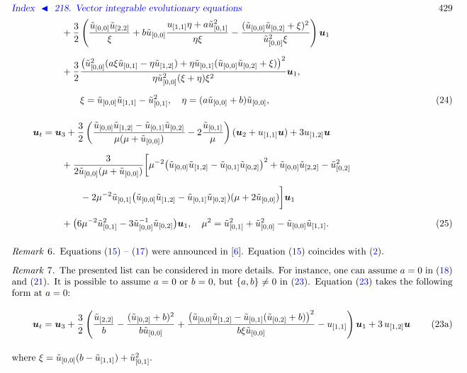
Index J 218. Vector integrable evolutionary equations 429

+3

2

(u[0,0]u[2,2]

ξ+ bu[0,0]

u[1,1]η + au2[0,1]

ηξ−

(u[0,0]u[0,2] + ξ)2

u2[0,0]ξ

)u1

+3

2

(u2

[0,0](aξu[0,1] − ηu[1,2]) + ηu[0,1](u[0,0]u[0,2] + ξ))2

ηu2[0,0](ξ + η)ξ2

u1,

ξ = u[0,0]u[1,1] − u2[0,1], η = (au[0,0] + b)u[0,0], (24)

ut = u3 +3

2

(u[0,0]u[1,2] − u[0,1]u[0,2]

µ(µ+ u[0,0])− 2

u[0,1]

µ

)(u2 + u[1,1]u) + 3u[1,2]u

+3

2u[0,0](µ+ u[0,0])

[µ−2

(u[0,0]u[1,2] − u[0,1]u[0,2]

)2+ u[0,0]u[2,2] − u2

[0,2]

− 2µ−2u[0,1]

(u[0,0]u[1,2] − u[0,1]u[0,2])(µ+ 2u[0,0])

]u1

+(6µ−2u2

[0,1] − 3u−1[0,0]u[0,2]

)u1, µ2 = u2

[0,1] + u2[0,0] − u[0,0]u[1,1]. (25)

Remark 6. Equations (15) – (17) were announced in [6]. Equation (15) coincides with (2).

Remark 7. The presented list can be considered in more details. For instance, one can assume a = 0 in (18)and (21). It is possible to assume a = 0 or b = 0, but a, b 6= 0 in (23). Equation (23) takes the followingform at a = 0:

ut = u3 +3

2

(u[2,2]

b−

(u[0,2] + b)2

bu[0,0]+

(u[0,0]u[1,2] − u[0,1](u[0,2] + b)

)2bξu[0,0]

− u[1,1]

)u1 + 3u[1,2]u (23a)

where ξ = u[0,0](b− u[1,1]) + u2[0,1].

Index J 218. Vector integrable evolutionary equations 430

The assumptions a = 0 and then b = 0 in (24) reduce this equation to the form

ut = u3 + 3

(u[0,1]

u[0,0]+u[0,1]u[0,2] − u[0,0]u[1,2]

ξ

)(u2 + u[1,1]u) + 3u[1,2]u

+3

2

(u[0,0]u[2,2]

ξ−

(ξ + u[0,0]u[0,2])2

ξu2[0,0]

)u1, ξ = u[0,0]u[1,1] − u2

[0,1]. (24a)

This is an anisotropic generalization of Schwarz-KdV equation.

5. Backlund transformations for equations on the sphere

All integrable equations on the sphere admits auto-Backlund transformations. These transformations containan arbitrary parameter which allows, in principle, to construct multisoliton and finite-gap solutions, even ifthe Lax representation is not known (see [11])

The first order Backlund auto-transformation for a scalar evolutionary equation is a relation between twosolutions u and v of this equation and their derivatives ux and vx. In the vector case, first order Backlundauto-transformation were introduced in the paper [6] as ODE of the form

u1 = fu+ gv + hvx (26)

where f, g and h are certain scalar function depending on the products of the vectors u,v and vx. Thearguments of f, g and h, in the case of isotropic equation in Rn, are

u[0,0] = (u,u), w0 = (u,v), w1 = (u,vx), v[0,0] = (v,v), v[0,1] = (v,vx), v[1,1] = (vx,vx).

In the anisotropic case, the products

u[0,0] = 〈u,u〉, w0 = 〈u,v〉, w1 = 〈u,vx〉, v[0,0] = 〈v,v〉, v[0,1] = 〈v,vx〉, v[1,1] = 〈vx,vx〉

should be added. The constraints eliminate the variables u[0,0], v[0,0] and v[0,1] in the case of equations onthe sphere or on a cone.

Index J 218. Vector integrable evolutionary equations 431

In order to find Backlund auto-transformation for the evolutionary equation (1) we differentiate (26) withrespect to t in virtue of equation (1) and then eliminate u1 by use of (26). By the definition of Backlundtransformation, the resulting equation must hold identically. The splitting of this equation with respectto those independent variables which do not occur as arguments of the functions f, g and h brings to anoverdetermined system on nonlinear PDE for these functions. If this system has a solution which dependessentially on the parameter λ then this solution defines the desired Backlund auto-transformation.

6. Divergent equations

The general classification problem for integrable equations (1) is very cumbersome and it is not solved atpresent. The coefficients of the equation depend on the large number of variables, but this is not the onlydifficulty. The known examples (see [12, 13]) demonstrate that the dependence of these coefficients on theirarguments can be extremely complicated.

The problem which leads to a quite visible answer is the classification of integrable vector evolutionaryequations of the form

ut = (u2 + f1u1 + f0u)x, fi = fi(u[0,0], u[0,0], u[0,1], u[0,1], u[1,1], u[1,1])

where fi are scalar functions. The list of such equations, obtained in [14] is as follows, after the transformationto the potential form by the change u→ u1:

ut = u3 +3

2

( a2u[1,2]2

1 + au[1,1]− au[2,2]

)u1, (27)

ut = u3 − 3u[1,2]

u[1,1]u2 +

3u[2,2]

3u[1,1]u1, (28)

ut = u3 − 3u[1,2]

u[1,1]u2 +

3

2

(u[2,2]

u[1,1]+

u[1,2]2

u[1,1]2(1 + au[1,1])

)u1, (29)

ut = u3 −3

2(p+ 1)

u[1,2]

pu[1,1]u2 +

3

2(p+ 1)

(u[2,2]

u[1,1]−au[1,2]

2

p2u[1,1]

)u1, (30)

Index J 218. Vector integrable evolutionary equations 432

ut = u3 − 3u[1,2]

u[1,1]u2 +

3

2

(u[2,2]

u[1,1]+u[1,2]

2

u[1,1]2

+ au[1,1]

u[1,1]

)u1, (31)

ut = u3 − 3u[1,2]

u[1,1]u2 + 3

u[2,2]

u[1,1]u1. (32)

Here p =√

1 + au[1,1] and a is a constant.It should be noted that the form of equations (28), (29), (31) and (32) coincide with the respective

equations on the sphere.

References

[1] I.Z. Golubchik, V.V. Sokolov. Multicomponent generalization of the hierarchy of the Landau–Lifshitz equation.Theor. Math. Phys. 124:1 (2000) 909–917.

[2] N.H. Ibragimov, A.B. Shabat. On infinite dimensional Lie–Backlund algebras. Funct. Anal. Appl. 14:4 (1980)79–80.

[3] S.I. Svinolupov, V.V. Sokolov. On evolution equations with nontrivial conservation laws. Funct. Anal. Appl.16:4 (1982) 86–87.

[4] V.V. Sokolov, A.B. Shabat. Classification of integrable evolution equations. Sov. Sci. Rev. C / Math. Phys. Rev.4 (1984) 221–280.

[5] A.V. Mikhailov, A.B. Shabat, V.V. Sokolov. The symmetry approach to classification of integrable equations.In: What is Integrability? (V.E. Zakharov ed). Springer-Verlag, 1991, pp. 115–184.

[6] A.G. Meshkov, V.V. Sokolov. Integrable evolution equations on the N -dimensional sphere. Commun. Math.Phys. 232:1 (2002) 1–18.

[7] V.V. Sokolov, S.I. Svinolupov. Vector-matrix generalizations of classical integrable equations. Theor. Math.Phys. 100 (1994) 959–962.

[8] S.I. Svinolupov, V.V. Sokolov. Deformations of Jordan triple systems and integrable equations. Theor. Math.Phys. 108:3 (1996) 1160–1163

[9] I.T. Habibullin, V.V. Sokolov, R.I. Yamilov. Multi-component integrable systems and nonassociative structures.pp. 139–168 in: Nonlinear Physics: Theory and Experiment, Lecce’95 (eds E. Alfinito, M. Boiti, L. Martina, F.Pempinelli) Singapore: World Scientific, 1996.

Index J 218. Vector integrable evolutionary equations 433

[10] M. Yu. Balakhnev, A.G. Meshkov. Integrable anisotropic evolution equations on a sphere. SIGMA 1 (2005) 027.

[11] V.E. Adler, A.B. Shabat, R.I. Yamilov. Symmetry approach to the integrability problem. Theor. Math. Phys.125:3 (2000) 1603–1661.

[12] M. Yu. Balakhnev, A.G. Meshkov. On a classification of integrable vectorial evolutionary equations. J. Nonl.Math. Phys. 15:2 (2008) 212–226.

[13] M. Yu. Balakhnev. On a class of integrable evolutionary vector equations. Theor. Math. Phys. 142:1 (2005)13–20.

[14] A.G. Meshkov, V.V. Sokolov. Classification of integrable divergent N -component evolution systems. Theor.Math. Phys. 139:2 (2004) 609–622.

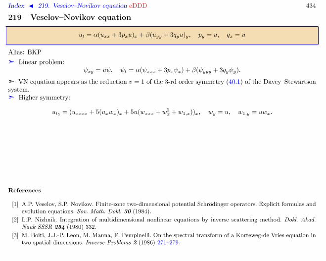
Index J 219. Veselov–Novikov equation eDDD 434

219 Veselov–Novikov equation

ut = α(uxx + 3pxu)x + β(uyy + 3qyu)y, py = u, qx = u

Alias: BKP

ã Linear problem:ψxy = uψ, ψt = α(ψxxx + 3pxψx) + β(ψyyy + 3qyψy).

ã VN equation appears as the reduction v = 1 of the 3-rd order symmetry (40.1) of the Davey–Stewartsonsystem.ã Higher symmetry:

ut5 = (uxxxx + 5(uxwx)x + 5u(wxxx + w2x + w1,x))x, wy = u, w1,y = uwx.

References

[1] A.P. Veselov, S.P. Novikov. Finite-zone two-dimensional potential Schrodinger operators. Explicit formulas andevolution equations. Sov. Math. Dokl. 30 (1984).

[2] L.P. Nizhnik. Integration of multidimensional nonlinear equations by inverse scattering method. Dokl. Akad.Nauk SSSR 254 (1980) 332.

[3] M. Boiti, J.J.-P. Leon, M. Manna, F. Pempinelli. On the spectral transform of a Korteweg-de Vries equation intwo spatial dimensions. Inverse Problems 2 (1986) 271–279.

Index J 220. Veselov–Novikov equation modified eDDD 435

220 Veselov–Novikov equation modified

ut = uxxx + 3uxwx +3

2uwxx, wy = u2

This is the reduction v = u of the 3-rd order symmetry (40.1) of the Davey–Stewartson system.

References

[1] L.V. Bogdanov. Veselov–Novikov equation as a natural two-dimensional generalization of the Korteweg-de Vriesequation. Theor. Math. Phys. 70:2 (1987) 219–223.

Index J 221. Volterra lattice eD∆ 436

221 Volterra lattice

un,x = un(un+1 − un−1) (1)

Aliases: Lotka–Volterra model, Kac-van Moerbeke lattice, Langmuir lattice.

ã Bi-Hamiltonian structure [5, 6, 7]:

un,x = un, H(1)1 = un, H(2)2,

un, un+11 = unun+1, H(1) =∑

un

un, un+12 = unun+1(un + un+1), un, un+22 = unun+1un+2, H(2) =1

2

∑log un

ã Backlund transformation:

un = (fn + δ)(fn+1 − δ), un = (fn+1 + δ)(fn − δ).

The variable f satisfies the modified Volterra lattice fn,x = (f2n − δ2)(fn+1 − fn−1).

ã Zero curvature representation:

Un =

(un −λun−λ λ2 + un−1

), Ln =

(λ un1 0

), Mn =

−λ

2δfn + δ

1

fn − δ− λ

fn − δ− λ

2δ

ã The lattice [8]

pn,x = pn(sn+1 − sn−1), −sn,x = sn(pn+1 − pn−1)

is splitted into two disjoint copies of the Volterra lattice (1) and un,x = un(un+1 − un−1) after the changeu2n = −p2n, u2n+1 = s2n+1, u2n = s2n, u2n+1 = −p2n+1.

ã Nonabelian generalization: let A be an associative algebra with unity, then the lattice [9]

un,x = un+1un − unun−1, un ∈ A

Index J 221. Volterra lattice eD∆ 437

admits the ZCR with the matrices Un,Wn of the same form as in scalar case. The simplest higher symmetrytakes the form

un,t = un+2un+1un + u2n+1un + un+1u

2n − u2

nun−1 − unu2n−1 − unun−1un−2.

ã Another multifield generalization [10, 11]:

u(j)n,x = u(j)

n

(j−1∑k=1

(u(k)n+1 − u(k)

n )−m∑

k=j+1

(u(k)n − u

(k)n−1)

), j = 1, . . . ,m

References

[1] V. Volterra. Lecons sur la theorie mathematique de la luttre pour la vie. Paris: Gauthier-Villars, 1931.

[2] M. Kac, P. van Moerbeke. On an explicitly soluble system of nonlinear differential equations related to certainToda lattices. Adv. in Math. 16:2 (1975) 160–169.

[3] V.E. Zakharov, S.L. Musher, A.M. Rubenchik. JETP Lett. 19:5 (1974) 249–253.

[4] S.V. Manakov. On the complete integrability and stochastization of discrete dynamical systems. Sov. Phys.JETP 40 (1974) 269–274.

[5] B.A. Kupershmidt. Discrete Lax equations and differential-difference calculus. Paris: Asterisque, 1985.

[6] L.D. Faddeev, L.A. Takhtajan. Liouville model on the lattice. Lect. Notes Phys. 246 (1986) 166–179.

[7] A.Yu. Volkov. Hamiltonian interpretation of the Volterra model. J. Sov. Math. 46 (1986) 1576–1581.

[8] S.B. Leble, M.A. Salle. Darboux transformation for the discrete analog of the Silin–Tikhonchuk equations. Dokl.Akad. Nauk SSSR 284:1 (1985) 110–114.

[9] M.A. Salle. Darboux transformations for nonabelian and nonlocal equations of the Toda lattice type. Theor.Math. Phys. 53:2 (1982) 227–237.

[10] Yu.B. Suris. Nonlocal quadratic Poisson algebras, monodromy map, and Bogoyavlensky lattices. J. Math. Phys.38 (1997) 4179–4201.

[11] Yu.B. Suris. The problem of integrable discretization: Hamiltonian approach. Basel: Birkhauser, 2003.

Index J 222. Volterra lattice modified eD∆ 438

222 Volterra lattice modified

un,x = (1− u2n)(un+1 − un−1)

Alias: discrete mKdV equation.

References

[1] A.K. Common. A solution of the initial value problem for half-infinite integrable lattice systems. Inverse Problems8 (1992) 393–408.

Index J 223. Volterra lattice twodimensional eDD∆ 439

223 Volterra lattice twodimensional

The version from [1, 2]:

ut = u(u2−1 − u2

1)± wy, (uu−1)y = uw−1 − u−1w

The version from [3, 4]:

ux = u(v − v1), vy = v(u− u−1)

References

[1] A.V. Mikhailov. Integrability of a two-dimensional generalization of the Toda chain. Sov. Phys. JETP Lett 30(1979) 414–418.

[2] A.V. Mikhailov. The reduction problem and the inverse scattering method. Physica D 3:1–2 (1981) 73–117.

[3] A.B. Shabat, R.I. Yamilov. To a transformation theory of two-dimensional integrable systems. Phys. Lett. A227:1–2 (1997) 15–23.

[4] E.V. Ferapontov. Laplace transformations of hydrodynamic-type systems in Riemann invariants: Periodic se-quences. J. Phys. A 30:19 (1997) 6861–6878.

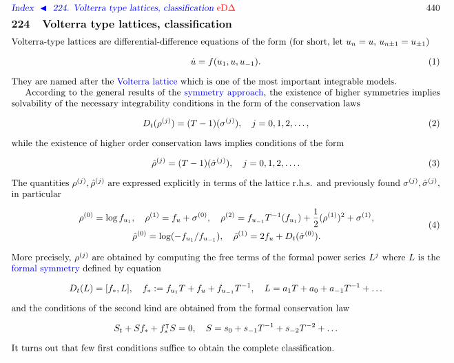
Index J 224. Volterra type lattices, classification eD∆ 440

224 Volterra type lattices, classification

Volterra-type lattices are differential-difference equations of the form (for short, let un = u, un±1 = u±1)

u = f(u1, u, u−1). (1)

They are named after the Volterra lattice which is one of the most important integrable models.According to the general results of the symmetry approach, the existence of higher symmetries implies

solvability of the necessary integrability conditions in the form of the conservation laws

Dt(ρ(j)) = (T − 1)(σ(j)), j = 0, 1, 2, . . . , (2)

while the existence of higher order conservation laws implies conditions of the form

ρ(j) = (T − 1)(σ(j)), j = 0, 1, 2, . . . . (3)

The quantities ρ(j), ρ(j) are expressed explicitly in terms of the lattice r.h.s. and previously found σ(j), σ(j),in particular

ρ(0) = log fu1 , ρ(1) = fu + σ(0), ρ(2) = fu−1T−1(fu1) +

1

2(ρ(1))2 + σ(1),

ρ(0) = log(−fu1/fu−1), ρ(1) = 2fu +Dt(σ(0)).

(4)

More precisely, ρ(j) are obtained by computing the free terms of the formal power series Lj where L is theformal symmetry defined by equation

Dt(L) = [f∗, L], f∗ := fu1T + fu + fu−1

T−1, L = a1T + a0 + a−1T−1 + . . .

and the conditions of the second kind are obtained from the formal conservation law

St + Sf∗ + fᵀ∗ S = 0, S = s0 + s−1T−1 + s−2T

−2 + . . .

It turns out that few first conditions suffice to obtain the complete classification.

Index J 224. Volterra type lattices, classification eD∆ 441

Theorem 1 (Yamilov [1]). The lattices (1) satisfying the necessary integrability conditions (2), (3) with thequantities given in (4) are exhausted, up to the point transformations u = a(u), by the following list:

u = P (u)(u1 − u−1) (5)

u = P (u2)( 1

u1 + u− 1

u+ u−1

)(6)

u = Q(u)( 1

u1 − u+

1

u− u−1

)(7)

u =H(u1, u, u−1) + ν(H(u1, u, u1)H(u−1, u, u−1))1/2

u1 − u−1, ν = 0,±1 (8)

u = f(u1 − u) + f(u− u−1), f ′ = P (f) (9)

u = f(u1 − u)f(u− u−1) + µ, f ′ = P (f)/f (10)

u = (f(u1 − u) + f(u− u−1))−1 + µ, f ′ = P (f2) (11)

u = (f(u1 + u)− f(u+ u−1))−1, f ′ = Q(f) (12)

u =f(u1 + u)− f(u+ u−1)

f(u1 + u) + f(u+ u−1), f ′ = P (f2)/f (13)

u =f(u1 + u) + f(u+ u−1)

f(u1 + u)− f(u+ u−1), f ′ = Q(f)/f (14)

u =(1− f(u1 − u))(1− f(u− u−1))

f(u1 − u) + f(u− u−1)+ µ, f ′ =

P (f2)

1− f2(15)

where P ′′′ = QV = 0 and H(u, v, w) = (αv2 + 2βv + γ)uw + (βv2 + λv + δ)(u+ w) + γv2 + 2δv + ε.All these lattices are integrable indeed, that is they belong to infinite hierarchies of commuting flows.

References

[1] R.I. Yamilov. On classification of discrete evolution equations. Usp. Mat. Nauk 38:6 (1983) 155–156.

Index J 224. Volterra type lattices, classification eD∆ 442

[2] A.V. Mikhailov, A.B. Shabat, R.I. Yamilov. The symmetry approach to classification of nonlinear equations.Complete lists of integrable systems. Russ. Math. Surveys 42:4 (1987) 1–63.

[3] R.I. Yamilov. Symmetries as integrability criteria for differential difference equations. J. Phys. A 39:45 (2006)R541–623.

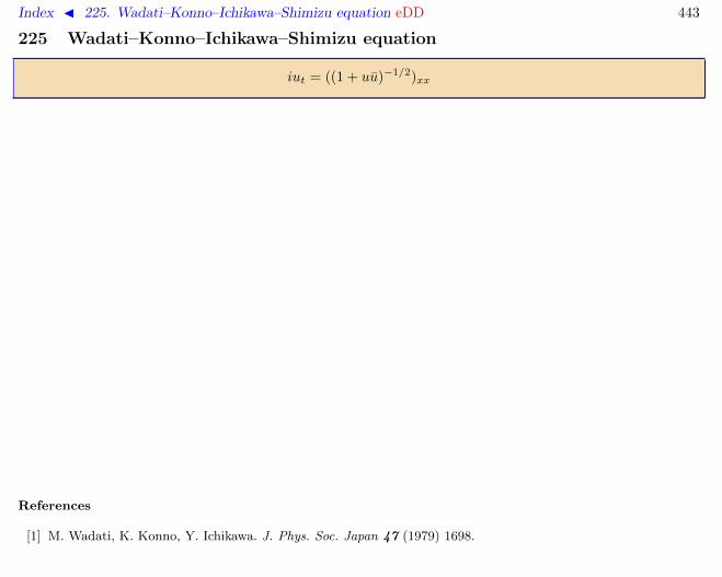
Index J 225. Wadati–Konno–Ichikawa–Shimizu equation eDD 443

225 Wadati–Konno–Ichikawa–Shimizu equation

iut = ((1 + uu)−1/2)xx

References

[1] M. Wadati, K. Konno, Y. Ichikawa. J. Phys. Soc. Japan 47 (1979) 1698.

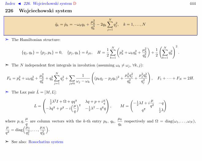
Index J 226. Wojciechowski system D 444

226 Wojciechowski system

qk = pk = −ωkqk +µ2k

q3k

− 2qk

N∑j=1

q2j , k = 1, . . . , N

ã The Hamiltonian structure:

qj , qk = pj , pk = 0, pj , qk = δjk, H =1

2

N∑k=1

(p2k + ωkq

2k +

µ2k

q2k

)+

1

2

(N∑k=1

q2k

)2

.

ã The N independent first integrals in involution (assuming ωk 6= ωj , ∀k, j):

Fk = p2k + ωkq

2k +

µ2k

q2k

+ q2k

N∑j=1

q2j +

∑j 6=k

1

ωj − ωk

((pkqj − pjqk)2 +

µ2kq

2j

q2k

+µ2jq

2k

q2j

), F1 + · · ·+ FN = 2H.

ã The Lax pair L = [M,L]:

L =

12λ

2I + Ω + qqᵀ λq + p+ iµq

−λqᵀ + pᵀ − i(µq

)ᵀ− 1

2λ2 − qᵀq

, M =

(− 1

2λI + iµ

q2−q

qᵀ 12λ

)

where p, q,µ

qare column vectors with the k-th entry pk, qk,

µkqk

respectively and Ω = diag(ω1, . . . , ωN ),

µ

q2= diag

(µ1

q21

, . . . ,µNq2N

).

ã See also: Rosochatius system

Index J 226. Wojciechowski system D 445

References

[1] S. Wojciechowski. Integrability of one particle in a perturbed central quartic potential. Phys. Scr. 31 (1985)433–438.

[2] Yu.B. Suris. Dynamical r-matrices for some nonlinear oscillators. J. Phys. A 28:3 (1995) L85–90.

[3] Yu.B. Suris. The problem of integrable discretization: Hamiltonian approach. Basel: Birkhauser, 2003.

Index J 227. Wronskian 446

227 Wronskian

Wide classes of explicit solutions to soliton equations, including rational, multi-soliton, multi-kink and others,possess a compact representation in terms of determinants. Each entry of such determinant is given by asimple expression corresponding in some way to a linear wave while the size of determinant depends on thenumber of poles of rational solution or the number of solitons. There are several types of such formulas relatedwith Wronsky, Gram or Casorati type determinants or Pfaffians (recall that the Pfaffian of skew-symmetricmatrix A of even order satisfies the relation Pf(A)2 = det(A)).

Pfaffianization is a certain procedure which allows to replace multi-soliton solutions represented bydeterminants with solutions represented by Pfaffians, in expense of adding some extra field variables into thesystem under scrutiny. This procedure was originally applied to Kadomtsev–Petviashvili equation, resultingin Hirota–Ohta system [3]. Later on, this procedure was applied to many other equations, see e.g. [4].

References

[1] M.M. Crum. Associated Sturm–Liouville systems. Quart. J. Math. Oxford Ser. 2 6 (1955) 121–127.

[2] Y. Ohta. Special solutions of discrete integrable systems. pp. 57–83 in: Discrete integrable systems (B. Gram-maticos, Y. Kosmann-Schwarzbach, T. Tamizhmani eds) Lect. Notes Phys. 644, Berlin: Springer-Verlag, 2004.

[3] R. Hirota, Y. Ohta. Hierarchies of coupled soliton equations. I. J. Phys. Soc. Japan 60 (1991) 798–809.

[4] C.R. Gilson. Generalizing the KP hierarchies: Pfaffian hierarchies. Theor. Math. Phys. 133:3 (2002) 1663–1674.

Index J 228. Yang–Baxter mappings 447

228 Yang–Baxter mappings

Author: V.E. Adler, 21.07.2005

1. 3D-consistency2. Yang–Baxter mappings on the linear pencils of conics3. Quadrirational mappings4. Multifield Yang–Baxter maps

Yang–Baxter maps, or set-theoretical solutions of Yang–Baxter equation [1] are 2D discrete equations whichsatisfy the property of 3D-consistency. A difference with the quad-equations is that the field variables areassociated with the edges of square lattice rather than the vertices.

1. 3D-consistency

Consider mappings Rij : Ci × Cj → Ci × Cj where Ci are some spaces or manifolds. Let the mapping

Rij : C1 × C2 × C3 → C1 × C2 × C3 act as Rij on i-th and j-th factors and be identical on the rest one.

Definition 1. Rij are called Yang–Baxter mappings if

R23 R13 R12 = R12 R13 R23

We will use also an alternative definition. Let Fij : Ci × Cj → Ci × Cj be given, in components, as

Fij : (xi, xj) 7→ (xij , xji ) = (f ij(x

i, xj), f ji (xj , xi)), i, j = 1, 2, 3, i 6= j.

Definition 2. The mappings Fij are called 3D-consistent if xijk ≡ xikj , that is

f ij(fik(xi, xk), f jk(xj , xk)) = f ik(f ij(x

i, xj), fkj (xk, xj)), i 6= j 6= k 6= i.

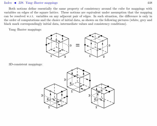
Index J 228. Yang–Baxter mappings 448

Both notions define essentially the same property of consistency around the cube for mappings withvariables on edges of the square lattice. These notions are equivalent under assumption that the mappingcan be resolved w.r.t. variables on any adjacent pair of edges. In such situation, the difference is only inthe order of computations and the choice of initial data, as shown on the following pictures (white, grey andblack mark correspondingly initial data, intermediate values and consistency conditions).

Yang–Baxter mappings:

1 2

3

1 2

3

3D-consistent mappings:

1

23

1

23

1

23

Index J 228. Yang–Baxter mappings 449

2. Yang–Baxter mappings on the linear pencils of conics

Let X1, X2 be points on conic sections C1, C2, respectively. Define the mapping F12 : C1 × C2 → C1 × C2

as follows:X1

2 = X1X2 ∩ C1, X21 = X1X2 ∩ C2.

C1

C2

112

2

21

Now let us consider the initial data on three conics from the linear pencil. On the first step we applythe mappings Fij : (Xi, Xj) 7→ (Xi

j , Xji ). Next, we apply the mappings once more and see the remarkable

incident theorem.

C1

C2

C3

112

13 123

2

21

23

213

3

31

32

312

Theorem 3. The mappings Fij are 3D-consistent: Xijk = Xi

kj.

Index J 228. Yang–Baxter mappings 450

Under a rational parametrization of the conics Ci : Xi = Xi(xi) the mapping F12 turns into a birationalmapping on CP1 × CP1. There exist 5 projective types of the linear pencils of conics Ci = C + aiK [2].These types lead to the following list of the mappings (i, j ∈ 1, 2):

xij = aixj (1− a2)x1 + a2 − a1 + (a1 − 1)x2

a2(1− a1)x1 + (a1 − a2)x2x1 + a1(a2 − 1)x2

xij =xj

ai· a1x

1 − a2x2 + a2 − a1

x1 − x2

xij =xj

ai· a1x

1 − a2x2

x1 − x2

xij = xj(

1 +a2 − a1

x1 − x2

)xij = xj +

a1 − a2

x1 − x2

(1)

The first one corresponds to the above figures with 4-point locus.

All these mappings can be obtained from those quad-equations listed in Theorem 187.3, which areinvariant with respect to the shift u→ u+ c or scaling u→ cu, by the changes xi = ui − u or xi = ui/u.

3. Quadrirational mappings

Definition 4 ([3, 4]). The mapping F : C1 × C2 → C1 × C2 is called quadrirational if it and the mappingsF (x1, ·) : C2 → C2, F (·, x2) : C1 → C1 for almost all xi ∈ Ci are birational isomorphisms.

x1

x2

x12

x21

F

F−1

x1

x2

x12

x21

@@@

@@I

F

@@@@@R

F−1

Index J 228. Yang–Baxter mappings 451

In the case C1 = C2 = CP1, a quadrirational mapping is of the form

F : x12 = f(x1, x2) =a(x2)x1 + b(x2)

c(x2)x1 + d(x2), x21 = g(x1, x2) =

A(x1)x2 +B(x1)

C(x1)x2 +D(x1)

with some special coefficients, such that the mappings F−1, F ,F−1 be of the same form.Assuming the nondegeneracy conditions

fx1gx2 − fx2gx1 6≡ 0, fx1 6≡ 0, fx2 6≡ 0, gx1 6≡ 0, gx2 6≡ 0,

one can prove that the coefficients can be at most quadratic polynomials. Moreover, the mapping F isdefined by the pair of polynomial equations

P (x2, x1, x21) = 0, Q(x2, x12, x21) = 0,

where either P,Q are linear in each argument or P,Q are linear in x2, x21 and quadratic resp. in x1, x12,and are related by formula

Q(x2, x12, x21) = (γx12 + δ)2P(x2,

αx12 + β

γx12 + δ, x21

).

Theorem 5. Up to the Mobius transformations, all nondegenerate quadrirational mappings, such thatmax deg(a, b, c, d) = max deg(A,B,C,D) = 2, are exhausted by the list (1).

4. Multifield Yang–Baxter maps

The geometric construction of Yang–Baxter maps works also on the linear pencil of quadrics. Indeed, allpoints lie on the plane defined by the initial data X1, X2, X3, so that 3D-consistency is inherited from theplanar situation. Nevertheless, the mapping itself cannot be reduced to the scalar one. Its general form is

Xij = Xj +

(ai − aj)(〈Xj , SXj〉+ 〈s,Xj〉+ σ)

〈Xi −Xj , (aiS + T )(Xi −Xj)〉(Xi −Xj)

where S, T are arbitrary symmetric matrices, s is an arbitrary vector and σ is an arbitrary scalar.Another examples of multifield Yang–Baxter maps were obtained in [5] by consideration of the interaction

of matrix solitons with the non-trivial internal parameters (vector analog of phase shift).

Index J 228. Yang–Baxter mappings 452

References

[1] V.G. Drinfeld. On some unsolved problems in quantum group theory. pp. 1–8 in Quantum groups, Lect. Notesin Mathematics 1510, Springer, 1992.

[2] M. Berger. Geometry. Berlin: Springer-Verlag, 1987.

[3] P. Etingof. Geometric crystals and set-theoretical solutions to the quantum Yang–Baxter equation. Preprintmath.QA/0112278.

[4] V.E. Adler, A.I. Bobenko, Yu.B. Suris. Geometry of Yang–Baxter maps: pencils of conics and quadrirationalmappings. Comm. Anal. and Geom. 12:5 (2004) 967–1007.

[5] A.P. Veselov. Yang–Baxter maps and integrable dynamics. Phys. Lett. A 314:3 (2003) 214–221.

Index J 229. Yang–Mills equation HD 453

229 Yang–Mills equation

(U−1Uz1)z1 + (U−1Uz2)z2 = 0

References

[1] M.J. Ablowitz, D.G. Costa, K. Tenenblat. Solutions of multidimensional extensions of the anti-self-dual Yang–Mills equation. Stud. Appl. Math. 77 (1987) 37–46.

Index J 230. Zakharov system eDD 454

230 Zakharov system

iψt = ψxx − nψ, nt = ux, ut = nx + (|ψ|2)x

This nonintegrable system describes the nonlinear interaction of two waves corresponding to the differenttime-spatial scales.

References

[1] A.V. Bocharov et al. Symmetries and conservation laws of the equations of mathematical physics. Moscow:Factorial, 1997. (in Russian)

Index J 231. Zero curvature repesentation 455

231 Zero curvature repesentation

A nonlinear equation admits the zero curvature representation (ZCR) if it is equivalent to the com-patibility condition of a pair of auxiliary linear problems. Partial differential, differential-difference anddifference-difference equations correspond to the following auxiliary problems:

DD : Ψx = UΨ, Ψt = VΨ ⇒ Ut = Vx + [V,U ]

D∆ : Ψn,x = UnΨn, Ψn+1 = LnΨn ⇒ Ln,x = Un+1Ln − LnUn∆∆ : Ψm,n+1 = Lm,nΨm,n, Ψm+1,n = Mm,nΨm,n ⇒ Mm+1,nLm,n = Lm,n+1Mm,n

where matrices depend on the variables of the equation, their derivatives or shifts, and the spectral parameterλ.

ã A ZCR is called trivial, if it can be reduced to the scalar one or the spectral parameter can be eliminated.

ã An important special case of ZCR is the Lax pair.

References

[1] V.E. Zakharov, A.B. Shabat. The scheme of integration of nonlinear equations of mathematical physics byinverse scattering method. I, II. Funct. Anal. Appl. 8:3 (1974) 226–235; 13:3 (1979) 166–174.

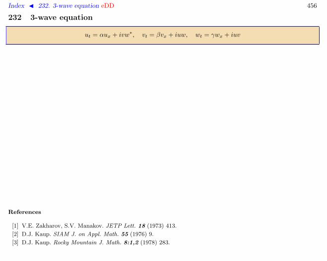
Index J 232. 3-wave equation eDD 456

232 3-wave equation

ut = αux + ivw∗, vt = βvx + iuw, wt = γwx + iuv

References

[1] V.E. Zakharov, S.V. Manakov. JETP Lett. 18 (1973) 413.

[2] D.J. Kaup. SIAM J. on Appl. Math. 55 (1976) 9.

[3] D.J. Kaup. Rocky Mountain J. Math. 8:1,2 (1978) 283.

Index J 233. ϕ4-equation hDD 457

233 ϕ4-equation

ϕxx − ϕtt = ±(ϕ− ϕ3)

References

[1] A.E. Kudryavtsev. Soliton-like collisions for a Higgs scalar field. Sov. Phys. JETP Lett. 22 (1975) 82–83.

[2] S. Aubry. A unified approach to the interpretation of displasive and order-disorder systems. II. J. Chem. Phys.64 (1976) 3392–3402.

[3] B.S. Getmanov. Sov. Phys. JETP Lett. 24 (1976) 291.

[4] V.G. Makhankov. Dynamics of classical solutions in non-integrable systems. Phys. Rep. 35 (1978) 1–128.

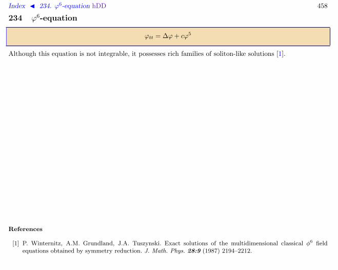
Index J 234. ϕ6-equation hDD 458

234 ϕ6-equation

ϕtt = ∆ϕ+ cϕ5

Although this equation is not integrable, it possesses rich families of soliton-like solutions [1].

References

[1] P. Winternitz, A.M. Grundland, J.A. Tuszynski. Exact solutions of the multidimensional classical φ6 fieldequations obtained by symmetry reduction. J. Math. Phys. 28:9 (1987) 2194–2212.