INFSO-ICT-248523 BeFEMTO D5 - European Commission · INFSO-ICT-248523 BeFEMTO ... presents the...
84
D5.3 Page 1 (84) INFSO-ICT-248523 BeFEMTO D5.3 Evaluation Report of Femtocells, Networking, Mobility and Management Solutions Contractual Date of Delivery to the CEC: M30 Actual Date of Delivery to the CEC: M30 Author(s): Tao Guo, Atta Quddus, Luis Cucala, Emilio Mino, Jaime Ferragut, José Nuñez-Martínez, Josep Mangues-Bafalluy, Miquel Soriano, Andrey Krendzel, Marc Portoles-Comeras, John Fitzpatrick, Nitin Maslekar, Marcus Schoeller, Frank Zdarsky, Mirosław Brzozowy, Zbigniew Kowalczyk, Konstantinos Samdanis Participant(s): NEC, TID, CTTC, UNIS, PTC Workpackage: WP5: Femtocells Access Control, Networking, Mobility and Management Estimated person months: 18.62 Security: PU Nature: R Version: 1.0 Total number of pages: 84 Abstract: This final WP5 deliverable presents the results of detailed simulation and analytical model based performance evaluation studies for the networking, mobility and management mechanisms and policies developed in this work package. Keywords: Traffic Offloading, Distributed Routing, Traffic Management, Resource Sharing, Location Management, Handover, Mobility Management, Access Control, Security, Networked Femtocells, Energy Efficiency, Distributed Fault Diagnosis Disclaimer: The information in this document is provided "as is", and no guarantee or warranty is given that the information is fit for any particular purpose. The user uses the information at its sole risk and liability.
Transcript of INFSO-ICT-248523 BeFEMTO D5 - European Commission · INFSO-ICT-248523 BeFEMTO ... presents the...

D5.3
Page 1 (84)
INFSO-ICT-248523 BeFEMTO
D5.3
Evaluation Report of Femtocells, Networking, Mobility and Management Solutions
Contractual Date of Delivery to the CEC: M30
Actual Date of Delivery to the CEC: M30
Author(s): Tao Guo, Atta Quddus, Luis Cucala, Emilio Mino, Jaime Ferragut, José
Nuñez-Martínez, Josep Mangues-Bafalluy, Miquel Soriano, Andrey
Krendzel, Marc Portoles-Comeras, John Fitzpatrick, Nitin Maslekar,
Marcus Schoeller, Frank Zdarsky, Mirosław Brzozowy, Zbigniew
Kowalczyk, Konstantinos Samdanis
Participant(s): NEC, TID, CTTC, UNIS, PTC
Workpackage: WP5: Femtocells Access Control, Networking, Mobility and Management
Estimated person months: 18.62
Security: PU
Nature: R
Version: 1.0
Total number of pages: 84
Abstract:
This final WP5 deliverable presents the results of detailed simulation and analytical model based
performance evaluation studies for the networking, mobility and management mechanisms and policies
developed in this work package.
Keywords:
Traffic Offloading, Distributed Routing, Traffic Management, Resource Sharing, Location Management,
Handover, Mobility Management, Access Control, Security, Networked Femtocells, Energy Efficiency,
Distributed Fault Diagnosis
Disclaimer:
The information in this document is provided "as is", and no guarantee or warranty is given that the
information is fit for any particular purpose. The user uses the information at its sole risk and liability.

D5.3
Page 2 (84)
Executive Summary
This document describes the final evaluation report for the schemes developed by BeFEMTO on the
traffic management, mobility management, network management, and security concepts in Work Package
5 (WP5). Some of them have already been proposed and described together with some initial evaluation
results in previous deliverable D5.2. This deliverable will present the final evaluation results following
the work in D5.2. In addition, as a final deliverable in WP5, this document also provides a summary for
all the solutions that have been developed within WP5 contributing to the BeFEMTO system concept as
presented in WP2.
Chapter 1 introduces the structure of this document and also provides a general overview of the technical
activities and achievements updated from D5.2.
Chapter 2 describes the activities related to traffic forwarding and resource sharing.
Chapter 3 presents the solutions and evaluation results for mobility management issues.
Chapter 4 deals with network management problems, in particular the energy management.
Chapter 5 focuses on security problems, in particular local access control in networks of femtocells for
multi-operator scenarios.
Chapter 6 summaries all the innovations and the achievements developed by BeFEMTO during the 2.5
year project phase.
D5.3
Page 3 (84)
List of Acronyms and Abbreviations
3GPP 3rd Generation Partnership Project
4G 4th Generation
AAA Authentication, Authorization, Accounting
ACK Acknowledgement
ACL Access Control List
AKA Authentication and Key Agreement
AP Access Point
API Application Programming Interface
BeFEMTO Broadband evolved FEMTO networks
CA Carrier Aggregation
CSG Closed Subscriber Group
CSS CSG Subscription Server
dB Decibel
dBm decibel (referenced to one milliwatt)
DL Downlink
DSCP Differentiated Services Code Point
EAP Extensible Authentication Protocol
eNB Evolved Node-B (LTE macro base station)
EPC Evolved Packet Core
EUTRAN Evolved Universal Terrestrial Radio Access Network
FAP Femto Access Point
FTTH Fibre To The Home
GHz Gigahertz
GPRS General Packet Radio Service
GTP GPRS Tunneling Protocol
HeNB Home evolved Node-B
HetNet Heterogeneous Networks
HLR Home Location Register
HNB Home Node-B
HO HandOver
HPLMN Home Public Land Mobile Network
HCSG HPLMN CSG Roaming
HSS Home Subscriber Server
IMS IP Multimedia Subsystem
IMSI International Mobile Subscriber Identity
IMT-ADV International Mobile Telephony – Advanced
IP Internet Protocol
ISD Inter Site Distance
ITU-R International Telecommunication Union-Radiocommunication Sector
ITU-T ITU-Telecommunication Standardization Sector
KPI Key Performance Indicator
LAN Local Area Network
LFGW Local Femtocell GateWay
LGW Local P-GW
LIPA Local IP access
LLM Local Location Management

D5.3
Page 4 (84)
LNO Local Network Operator
LTE 3GPP Long Term Evolution
MAC Media Access Control
MBMS Multimedia Broadcast Multicast System
MHz Mega Hertz
MME Mobility Management Entity
MNO Mobile Network Operator
MSISDN Mobile Subscriber Integrated Services Digital Network Number
NAS Non-Access Stratum
NASS Network Access Support Subsystem
NoF Network of Femtocells
ns Nanosecond
OMA DM Open Mobile Alliance Device Management
P-MME Proxy Mobility Management Entity
QoS Quality of Service
RACS Remote Access Control Subsystem
RADIUS Remote Authentication Dial in User Server
RSRP Reference Signal Received Power
SCTP Stream Control Transmission Protocol
S-GW Serving GateWay
SINR Signal to Interference plus Noise Ratio
SIPTO Selected IP Traffic Offload
SIT Service Interruption Time
SP Strict Priority
S-TMSI Serving Temporary Mobile Subscriber Identity
TA Tracking Area
TAL Tracking Area List
TAU Tracking Area Update
TEID Tunnel End-point IDentifier
TME Traffic Management Entity
TTL Time-to-Live
UE User Equipment
UICC Universal Integrated Circuit Card
UL Uplink
UMTS Universal Mobile Telecommunication System
UTRA Universal Terrestrial Radio Access
UTRAN Universal Terrestrial Radio Access Network
VBR Variable Bit Rate
VLAN Virtual LAN
VLTAG VLAN Tag
VoIP Voice over Internet Protocol
VPLMN Visited Public Land Mobile Network
VCSG VPLMN Autonomous CSG Roaming
WFQ Weighted Fair Queuing
WID Work Item Description
WP Work Package

D5.3
Page 5 (84)
Authors
Partner Name Phone / Fax / e-mail
NEC John Fitzpatrick email: [email protected]
Nitin Maslekar Phone: +49 6221 4342 213
email: [email protected]
Konstantinos Samdanis Phone: +49 6221 4342 225
email: [email protected]
Marcus Schoeller Phone: +49 6221 4342 217
email: [email protected]
Frank Zdarsky Phone: +49 6221 4342 142
email: [email protected]
Telefonica I+D Luis Cucala, Phone: +34 91 3128799
e-mail: [email protected]
Emilio Mino Phone: +34 91 3128799
e-mail: [email protected]
PTC Mirosław Brzozowy Phone: +48 224135881
e-mail:[email protected]
Zbigniew Kowalczyk Phone: +48 224136741
e-mail:[email protected]
CTTC José Núñez Phone: +34 93 645 29 00
e-mail: [email protected]
Jaime Ferragut Phone: +34 93 645 29 00, ext. 2113
e-mail: [email protected]
Josep Mangues Phone: +34 93 645 29 00
e-mail: [email protected]
Andrey Krendzel Phone: +34 93 645 29 16
e-mail: [email protected]
Marc Portoles Phone: +34 93 645 29 00
e-mail: [email protected]
Miquel Soriano e-mail: [email protected]
University of Surrey Tao Guo Phone: +44 1483 689485
e-mail: [email protected]
Atta ul Quddus Phone: +44 1483 683787
e-mail: [email protected]

D5.3
Page 6 (84)
Table of Contents
1. Introduction ............................................................................................... 10
1.1 Scope ......................................................................................................................................... 10 1.2 Organisation and Overview ....................................................................................................... 10 1.3 Contributions ............................................................................................................................. 10
2. Traffic Forwarding and Resource Sharing .............................................. 12
2.1 Centralized Traffic Management for Cooperative Femtocell Networks .................................... 12 2.1.1 Evaluation scenarios ......................................................................................................... 13 2.1.2 Simulation Analysis .......................................................................................................... 16 2.1.3 Conclusion and Future work ............................................................................................. 22
2.2 Distributed Routing ................................................................................................................... 22 2.2.1 Work during Year 2 .......................................................................................................... 22 2.2.2 Variable-V algorithm: Final Solution and Evaluation ....................................................... 23 2.2.3 Multi Local Femto Gateway ............................................................................................. 29 2.2.4 Dead Ends ......................................................................................................................... 36 2.2.5 Conclusions ....................................................................................................................... 40
2.3 Traffic Offloading ..................................................................................................................... 41 2.3.1 Introduction ....................................................................................................................... 41 2.3.2 Work during Year 2 .......................................................................................................... 41 2.3.3 Main Results ..................................................................................................................... 42 2.3.4 Conclusion ........................................................................................................................ 47
3. Mobility Management ................................................................................ 48
3.1 Local Location Management ..................................................................................................... 48 3.1.1 Introduction ....................................................................................................................... 48 3.1.2 Work during Years 1 and 2 ............................................................................................... 48 3.1.3 Enhancements to Proposed Schemes ................................................................................ 51 3.1.4 Performance Evaluation .................................................................................................... 56
3.2 Seamless Macro-Femto Handover Based on Reactive Data Bicasting ...................................... 56 3.2.1 Introduction ....................................................................................................................... 56 3.2.2 Proposed Handover Procedure .......................................................................................... 56 3.2.3 KPI Analysis ..................................................................................................................... 58 3.2.4 Numerical Results ............................................................................................................. 60 3.2.5 Conclusion ........................................................................................................................ 61
4. Network Management ............................................................................... 63
4.1 Energy Saving Network Management and Performance in HetNets ......................................... 63 4.1.1 Current macro-only deployment limitations ..................................................................... 63 4.1.2 Macrocell coverage analysis from the energy efficiency point of view ............................ 63 4.1.3 Combined macro and femto coverage analysis from the energy efficiency point of view 64 4.1.4 Strategies to reduce energy consumption and interference in the femtonode layer .......... 67
5. Security ...................................................................................................... 68
5.1 Local access control in networks of femtocells for multi-operator scenarios ............................ 68 5.1.1 Introduction ....................................................................................................................... 68 5.1.2 Work during Year 2 .......................................................................................................... 68 5.1.3 Relevant building blocks and interfaces ............................................................................ 69 5.1.4 Relevant procedures .......................................................................................................... 69 5.1.5 Updated MSC of local access control for multi-operator scenario ................................... 72 5.1.6 Comments on local access control options........................................................................ 73
6. Summary of WP5 Findings ....................................................................... 74
6.1 Traffic Forwarding and Resource Sharing................................................................................. 74 6.1.1 Centralized Traffic Management for Cooperative Femtocell Networks ........................... 74 6.1.2 Distributed Routing ........................................................................................................... 74

D5.3
Page 7 (84)
6.1.3 Voice Call Capacity Analysis of Long Range WiFi as a Femto Backhaul Solution ......... 75 6.1.4 Local Breakout for Networked Femtocells ....................................................................... 75 6.1.5 Traffic Offloading ............................................................................................................. 76 6.1.6 A QoS based call admission control and resource allocation mechanism for LTE
femtocell deployment........................................................................................................ 76 6.2 Mobility Management ............................................................................................................... 77
6.2.1 Local Mobility Management ............................................................................................. 77 6.2.2 Local Location Management ............................................................................................. 77 6.2.3 Mobility Management for Networked Femtocells Based on X2 Traffic Forwarding ....... 78 6.2.4 Inbound/Outbound Mobility Optimization ....................................................................... 78 6.2.5 Seamless Macro-Femto Handover Based on Reactive Data Bicasting ............................. 78 6.2.6 Mobile Femtocells based on Multi-homing Femtocells .................................................... 79 6.2.7 Deployment, Handover and Performance of Networked Femtocells in an Enterprise LAN79
6.3 Network Management ............................................................................................................... 80 6.3.1 Distributed Fault Diagnosis ............................................................................................... 80 6.3.2 Energy Saving and Performance in HetNets ..................................................................... 80 6.3.3 Enhanced Power Management in Femtocell Networks ..................................................... 80
6.4 Security ...................................................................................................................................... 81 6.4.1 Secure, Loose-Coupled Authentication of the Femtocell Subscriber ................................ 81 6.4.2 Access Control to Local Network and Services ................................................................ 81 6.4.3 Architecture and IP Security ............................................................................................. 82
6.5 Revenue Sharing in Multi-Stakeholder Scenarios ..................................................................... 82
7. References ................................................................................................. 83

D5.3
Page 8 (84)
Table of Figures
Figure 2-1 Enterprise femto network .......................................................................................................... 13 Figure 2-2 SP within VLAN and WFQ between VLANs .......................................................................... 14 Figure 2-3 WFQ within VLAN and SP between VALNs .......................................................................... 14 Figure 2-4 Centralized Routing Based on OpenFlow ................................................................................. 15 Figure 2-5 Packet Loss in baseline scenario ............................................................................................... 18 Figure 2-6 End-End Delay in baseline scenario ......................................................................................... 19 Figure 2-7 Packet Loss with priority .......................................................................................................... 19 Figure 2-8 End-End Delay with priority ..................................................................................................... 20 Figure 2-9 Packet Loss in VLB based scenario .......................................................................................... 21 Figure 2-10 End-End Delay in VLB based scenario .................................................................................. 21 Figure 2-11 Illustration of the calculation of the variable value of V ......................................................... 24 Figure 2-12 Per-packet V calculation as a function of TTL ....................................................................... 26 Figure 2-13 Throughput and Packet Delivery Ratio for VarPrev-V and Var-V algorithms ....................... 27 Figure 2-14 Comparison of Delay and Packet Delay Distribution for VarPrev-V and Var-V algorithms . 28 Figure 2-15 Throughput vs. load/number of flows for VarPrev-V and Var-V algorithms ......................... 28 Figure 2-16 End-to-end delay vs. load/number of flows for VarPrev-V and Var-V algorithms ................ 29 Figure 2-17 Multi Local Femto Gateway ................................................................................................... 30 Figure 2-18 Reduction in terms of congestion introduced by adding an opportunistic LFGW .................. 30 Figure 2-19 Comparison between different routing variants (fixed-V and variable-V routing policies) in
terms of Aggregated Throughput with 1 LFGW and 2 LFGWs ................................................................. 31 Figure 2-20 Comparison between different routing variants (i.e., fixed-V and variable-V routing variants)
in terms of End-to-end delay with 1 LFGW and 2 LFGWs. ...................................................................... 32 Figure 2-21 Comparison between different routing variants in terms of Packet Delivery Ratio ................ 32 Figure 2-22 Different routing variants (i.e., fixed-V and variable-V) in terms of aggregated throughput
with 1 LFGW ............................................................................................................................................. 33 Figure 2-23 Different routing variants (i.e., fixed-V and variable-V) in terms of aggregated throughput
with 3 LFGWs ............................................................................................................................................ 33 Figure 2-24 Different routing variants (i.e., fixed-V and variable-V) in terms of aggregated throughput
with 5 LFGWs ............................................................................................................................................ 34 Figure 2-25 Different routing variants in terms of Delay 1 LFGW ............................................................ 34 Figure 2-26 Different routing variants in terms of PDR 1 LFGW ............................................................. 35 Figure 2-27 Different routing variants in terms of Delay 3 LFGWs .......................................................... 35 Figure 2-28 Different routing variants in terms of PDR 3LFGWs ............................................................. 35 Figure 2-29 Different routing variants in terms of Delay with 5 LFGWs .................................................. 35 Figure 2-30 Different routing variants in terms of PDR 5 LFGWs ............................................................ 36 Figure 2-31 Heatmaps illustrating the light hole problem with the Var-V algorithm. ............................... 37 Figure 2-32 Attained throughput after switching off 3 HeNBs .................................................................. 38 Figure 2-33 Delay Distribution of Packets for routing variants able to circumvent the hole ..................... 38 Figure 2-34 Packet Delivery Ratio for routing variants able to circumvent the hole ................................. 38 Figure 2-35 Illustration of the operation of Var-V and fixed-V algorithms in the presence of obstacles... 38 Figure 2-36 Achieved throughput with fixed V and var-V algorithms in the presence of obstacles .......... 39 Figure 2-37 Packet delay distribution attained with fixed V and var-V algorithms in the presence of
obstacles ..................................................................................................................................................... 39 Figure 2-38 Packet delivery ratio with fixed V and var-V algorithms in the presence of obstacles ........... 39 Figure 2-39 Illustration of the operation of Var-V algorithm with complex obstacles ............................... 40 Figure 2-40: Non-offloaded traffic from a single source (Z(t)) modelled as product of two strictly
alternating ON/OFF processes, X(t) and Y(t) ............................................................................................. 42 Figure 2-41: Estimation of the tail-index
zmin by means of Hill’s estimator when
zmin=
zoff .................. 43
Figure 2-42: Estimation of the tail-index zon by means of Hill’s estimator .............................................. 44
Figure 2-43: Estimation of the tail-index zon by means of Hill’s estimator when
zmin=
zon ................... 44
Figure 2-44: Bounds on resource needs vs. variance coefficient (a) with 50% of offloaded traffic .......... 45 Figure 2-45: Normalized overprovisioning of the system taking a fluid model approximation ................. 46 Figure 2-46: Illustration of the relation between the parameters of the system and the required capacity
before and after implementing offloading .................................................................................................. 46 Figure 3-1: The 2.5 Layer (Geosublayer) in the LLM Protocol Architecture. ........................................... 49 Figure 3-2: Impact of UE speed on location signalling traffic (static vs. dynamic TALs) ......................... 50 Figure 3-3: Operation of the Standard vs. Distributed Paging Mechanisms .............................................. 52 Figure 3-4: Proposed handover procedure .................................................................................................. 57 Figure 3-5: Handover from macrocell to femtocell. ................................................................................... 61

D5.3
Page 9 (84)
Figure 3-6: Handover from femtocell to macrocell. ................................................................................... 61 Figure 4-1. Available throughput map in the reference scenario ................................................................ 64 Figure 4-2. Reference 80 m2 apartment scenario with a central femtonode .............................................. 64 Figure 4-3. Femtocell Type III throughput map ......................................................................................... 66 Figure 5-1: CSG provisioning for roaming UEs involving the CSS .......................................................... 70 Figure 5-2: Access control at the MNO-level based on CSG subscription information retrieved from the
CSS ............................................................................................................................................................. 70 Figure 5-3: MSC for establishing PDN connectivity with LIPA/SIPTO support and local access control 72

D5.3
Page 10 (84)
1. Introduction
1.1 Scope
During year 1 and year 2 of the BeFEMTO project, Work Package (WP) 5 have developed a number of
innovative concepts, mechanisms and evaluations in the area of traffic management, mobility
management, security and network management of standalone, networked femtocells and mobile relay
femtocells. These are described in the deliverable D5.1 [1] and D5.2 [2].
As a final deliverable, this deliverable will present the final evaluation results following the work in D5.2.
In addition, this document also provides a summary for all the solutions that have been developed within
WP5 contributing to the BeFEMTO system concept, as presented in WP2 D2.3 [3].
Finally, it is worth noting that WP5’s scope is the research, development, and experimentation of novel
femtocell technologies, but that detailed descriptions of the implementation of these technologies for the
testbeds is outside WP5’s scope, but is instead addressed by WP6 and documented in the its respective
deliverables.
1.2 Organisation and Overview
The present deliverable is organised as follows:
Chapter 2 groups the work items related to the traffic forwarding of user and control plane traffic within a
network of femtocells and to the sharing of that network’s forwarding resources.
Chapter 3 presents the work items related to mobility management
Chapter 4 contains the work items related to the management of BeFEMTO femtocells in particular for
energy saving.
Chapter Error! Reference source not found. is concerned with local access control in networks of
femtocells for multi-operator scenarios.
Chapter 6 finally summarizes all the innovations made by BeFEMTO in WP5 during the whole project
phase contributing towards the BeFEMTO system concepts
1.3 Contributions
During the last half year of the project, WP5 has made the following achievements and contributions:
The geographic+backpressure distributed routing protocol has been enhanced with a variable-V algorithm
able to obtain an interesting trade-off between throughput, delay, and packet delivery ratio. Specifically,
we propose a variable-V algorithm that dynamically adapts the weight of Lyapunov drift-plus-penalty
routing decisions on a per-packet basis. The specific V parameter is function of the traffic load around the
HeNB, and the number of hops traversed by data packets. On the other hand, the proposed routing
protocol has been shown to be appropriate in the multi-LFGW scenario, and to overcome holes in sparse
deployments, whilst still retaining its main features. We proposed a deployment strategy for multiple
LFGW. The main advantage observed is the decrease of congestion in the Network of Femtocells (NoF)
with respect to single LFGW NoF deployments, yielding to improvements in throughput, delay, and
packet delivery ratio. Finally, we evaluated the distributed routing protocol under several sparse
deployments. The study indicates the convenience of using the variable-V routing scheme to circumvent
holes compared to fixed-V routing policies.
A paper presenting the distributed routing protocol for any-to any- traffic pattern with the use of the
variable-V algorithm (i.e., uplink, downlink, and local routing) has been accepted for publication in
IEEE HOTMESH WORKSHOP 2012.
Analysis of the voice call capacity of long range WiFi as a femtocell backhaul solution has been studied.
A paper presenting this analysis has been submitted to the IEEE Journal on Selected Areas in
Communications.
Numerical evaluation of the local mobility management and traffic offload solutions described earlier in
D5.1[1] has been carried out, illustrating their benefits in terms of reducing signalling and data traffic
load on the backhaul links and mobile core networks. In addition, an analytical framework for traffic

D5.3
Page 11 (84)
modelling in mobile networks implementing offloading has been developed and performance bounds of
the resource consumption in networks implementing offloading have been determined. These can be used
for network dimensioning. Comparison of the required network resources before and after deploying
offloading for providing a given quality of service has also been investigated.
A paper presenting this analysis has been submitted to the IEEE Journal on Selected Areas in
Communications.
Design of a QoS based call admission control and resource allocation mechanism for LTE femtocell
deployments and the evaluation of this mechanism.
A paper presenting this mechanism and its evaluation has been submitted to the IEEE Consumer
Communications & Networking Conference (CCNC) 2012.
Design of a self-organized tracking area list (TAL) mechanism for large-scale networks of femtocells.
The aim of this proposal is to improve the accuracy of standard 3GPP location management schemes,
while reducing the signalling traffic over the network of femtocells. This mechanism allows MMEs/P-
MMEs to provide UEs with adaptive TALs depending on their mobility state and, eventually, current
network conditions.
A paper presenting this mechanism and its evaluation has been presented in IEEE International
Conference on Communications (ICC) 2012.
A paper on Mobility management for large-scale all-wireless networks of femtocells in the Evolved
Packet System has been submitted to a special issue on Femtocells in 4G Systems of the EURASIP
Journal on Wireless Communications and Networking.
A chapter of a Wiley book on Heterogeneous Networks (HetNets) on Mobility management for
large-scale all-wireless networks of femtocells has been accepted for publication.
A paper on Traffic and mobility management in Networks of Femtocells has been submitted to a
special issue on Networked Femtocells of the ACM/Springer Journal on Mobile Networks and
Applications (MONET).As of the time of writing this deliverable, we are reviewing it, based on the
comments received.
Design of a distributed paging mechanism to reduce over-the-air (OTA) paging signalling traffic in large-
scale, all-wireless NoFs. The proposed scheme leverages the standard 3GPP X2 interface between
femtocells to propagate paging messages efficiently throughout the wireless multihop backbone.
A paper presenting this mechanism and its evaluation is going to be submitted in brief.
Design of a novel seamless handover procedure for user mobility from a macrocell to a femtocell and vice
versa. In this scheme, downlink data received at S-GW is bicasted to both the source cell and the target
cell after the handover procedure is actually imitated by the source cell. The proposed scheme has
significantly reduced the downlink service interruption time while still avoiding the packet loss during
handover
A paper presenting the proposed seamless handover procedure based on reactive data bicasting
and the performance evaluation has been submitted to IEEE Communications Letters.
Study on the implementation of networked femtonodes in an enterprise LAN including the LAN
configuration changes that are needed to support the networked femtocell group as well as the logical
connectivity of the networked femtonodes group to their corresponding femtonode subsystem.
Additionally, networked femtonode radio planning, and analysis of effective radio coverage has also been
carried out.
Study on procedures to reduce the interference level and the aggregated power consumption in a
heterogeneous network deployment that combines a macro layer and a small cell layer served by indoor
femtonodes. These procedures involve the power reduction of the macro layer thanks to the indoor
service provisioning from the femtonodes, and the switching off of those femtonodes that are not
providing any traffic when the users are not at their premises.

D5.3
Page 12 (84)
2. Traffic Forwarding and Resource Sharing
This chapter reports on results of BeFEMTO’s work on traffic forwarding and resource sharing from the
last half year of the project.
Sections 2.1 and 2.2 present extended results of prior work on traffic handling in networks of femtocells,
i.e. how to efficiently forward traffic between femtocells and femtocell gateway or between femtocells,
given that the transport network is a shared resource. Section 2.1 reports on results from the centralized
traffic management case, in which forwarding is controlled by a Local Femtocell Gateway (LFGW) that
has a complete view of the network. Focus is on the question how femtocell and non-femtocell traffic can
share the common local networking resources efficiently. Section 2.2 then reports on extensions of the
distributed backpressure routing algorithm that has been designed for the more challenging case of all-
wireless networks of femtocells. Extensions are presented for auto-tuning this algorithm and for making it
capable of working with multiple LFGWs and routing holes.
Section 2.3 then presents results from a complete study on traffic offloading, which was initially
introduced in D5.2. In particular, it studies the effect that opportunistic offloading has on the load and
characteristics of the remaining traffic that is still routed via the core network and the consequences this
has on network dimensioning.
2.1 Centralized Traffic Management for Cooperative Femtocell Networks
In co-operative femto networks, management of femtocells, including cell provisioning and traffic
prioritization, must be handled carefully. In addition to managing the femto traffic, it is also necessary to
guarantee that femto traffic is not affected by the presence of non-femto traffic and vice versa. To
provision this, either a separate IP network can be provided for femtocells or the femto traffic can be
overlaid onto the existing internal network and provide strategies to manage the traffic.
In this context, a potential solution in co-operative femto networks is to provision packets on centralized
flow based mechanisms. In flow-based strategies, packets are forwarded based on explicit forwarding
state installed in the forwarding elements, allowing the network to be “traffic engineered” for higher
resource utilizations. They also allow for a finer control on how network resources are shared between
flows. Depending on the classifier used for forwarding, flows-based mechanisms can handle anything
from micro flows to aggregate flows, even concurrently.
The current work focuses on networked femtocells case in general and an enterprise network in particular.
The target is to design mechanisms necessary to allow resource-efficient traffic forwarding within the co-
operative femto networks.
D5.3
Page 13 (84)
UEFemtocell Enterprise
Switch
LFGW Enterprise Server
(background traffic)
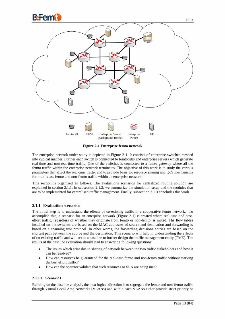
Figure 2-1 Enterprise femto network
The enterprise network under study is depicted in Figure 2-1. It consists of enterprise switches meshed
into cubical manner. Further each switch is connected to femtocells and enterprise servers which generate
real-time and non-real-time traffic. One of the switches is connected to a femto gateway where all the
femto traffic within the enterprise network terminates. The objective of this work is to study the various
parameters that affect the real-time traffic and to provide basis for resource sharing and QoS mechanisms
for multi-class femto and non-femto traffic within an enterprise network.
This section is organized as follows. The evaluations scenarios for centralized routing solution are
explained in section 2.1.1. In subsection 2.1.2, we summarize the simulation setup and the modules that
are to be implemented for centralised traffic management. Finally, subsection 2.1.3 concludes this work.
2.1.1 Evaluation scenarios
The initial step is to understand the effects of co-existing traffic in a cooperative femto network. To
accomplish this, a scenario for an enterprise network (Figure 2-1) is created where real-time and best-
effort traffic, regardless of whether they originate from femto or non-femto, is mixed. The flow tables
installed on the switches are based on the MAC addresses of source and destination and forwarding is
based on a spanning tree protocol. In other words, the forwarding decisions entries are based on the
shortest path between the source and the destination. This scenario will help in understanding the effects
of co-existing traffic and will act as a baseline to further design the traffic management entity (TME). The
results of the baseline evaluation should lead to answering following questions:
The issues which arise due to sharing of network between the two traffic stakeholders and how it
can be resolved?
How can resources be guaranteed for the real-time femto and non-femto traffic without starving
the best effort traffic?
How can the operator validate that such resources or SLA are being met?
2.1.1.1 Scenario1
Building on the baseline analysis, the next logical direction is to segregate the femto and non-femto traffic
through Virtual Local Area Networks (VLANs) and within each VLANs either provide strict priority or

D5.3
Page 14 (84)
weighted fair queuing (WFQ) mechanism. The forwarding paths are still based on shortest path
algorithms. This can be achieved in two ways which are described below.
Case1: Strict Priority between real-time / non-real-time traffic and WFQ between femto and Non-
femto traffic.
This case is shown in Figure 2-2, where a strict priority mechanism is implemented within each VLAN.
This approach will ensure that the real time traffic within femto and non-femto network is treated with
high priority so as to minimize the latency.
SP
WFQ
SP
Femto Traffic
Non Femto Traffic
Figure 2-2 SP within VLAN and WFQ between VLANs
This implementation can help to treat the real-time traffic within femto and non-femto domain efficiently.
However, WFQ between femto and non-femto traffic might lead to an overall degradation in the
performance. Such degradation can be frequent if most of the non-femto traffic is best effort. Under this
context, the real-time femto traffic might have to wait for a longer duration in the queue which results into
an increased latency.
Case2: WFQ between real-time / non-real-time traffic and Strict Priority between femto and Non-
femto traffic.
To overcome the drawback in previous method, as shown in Figure 2-3, we reverse the queuing principle
and apply WFQ within the VLAN and then adopt a strict priority.
WFQ
SP
WFQ
Femto Traffic
Non Femto Traffic
Figure 2-3 WFQ within VLAN and SP between VALNs
This method will work well if the problem mentioned is case 1 is persistent. However, there might be
issue which arises when both femto and non-femto are dominant in real-time traffic. This issue can be
addressed if we adopt an arbitrary routing mechanism within the enterprise network which will find
suitable paths for real-time femto and non-femto traffic.

D5.3
Page 15 (84)
2.1.1.2 Scenario 2
In this scenario the traffic management will be based on fixed resource allocation method. This allocation
can be based on flow tuples which can constitute a) (src_ip, dst_ip) tuple or b) (src_ip, dst_ip, dscp). The
queuing mechanism utilised will be the same as scenario 1. However, fixed resource allocation may lead
to following disadvantages:
chronic underutilization of resources,
highly restricted bandwidth for both enterprise and femto traffic,
insufficient flexibility under conditions of increasing load.
The magnitude of these will be analysed and based on this analysis we propose a load balancing
mechanism.
2.1.1.3 Scenario 3
The function or entity performing the routing for flows needs to be aware of a) the capacity on each link
of the topology and b) the traffic within the network which includes the femto and non-femto traffic.
Under these requirements a distributed approach for traffic engineering and routing would require a large
signalling overhead to disseminate this information to all routing functions and would be more complex
and thus more error-prone to implement. It therefore seems logical to take a centralized approach, in
which traffic engineering and routing is performed within a single “routing controller” function that then
installs paths with the forwarding entities in the network.
Based on the analysis of scenario 2, the logical direction for centralized routing in cooperative femto
networks would be to introduce dynamic resource allocation mechanisms. Under this scope, in this work,
we propose to implement and evaluate a centralized routing based on load-balancing architecture using
OpenFlow switches which are connected to a common controller.
OpenFlow was created in 2008 by a team from Stanford University. OpenFlow switches are like a
standard hardware switch with a flow table performing packet lookup and forwarding. However, the
difference lies in how flow rules are inserted and updated inside the switch’s flow table. A standard
switch can have static rules inserted into the switch or can be a learning switch where the switch inserts
rules into its flow table as it learns on which interface (switch port) a machine is. The OpenFlow switch
on the other hand uses an external controller to add rules into its flow table. These rules can be based on
more fine-granular identifier like QoS requirements, which will help in selecting the next forwarding hop
and to route the femto and non-femto traffic efficiently within cooperative femto networks (Figure 2-4).
Figure 2-4 Centralized Routing Based on OpenFlow

D5.3
Page 16 (84)
As evident, the load balancing strategies in an OpenFlow based environment has to be designed at the
controller to which the switches are connected. This design is governed by the following criterions:
What kind of information does the controller require and where does it get it from?
In an OpenFlow based solution the controller is responsible to install flow tables in the switches.
To make an efficient decision the controller requires a constant influx of flow requirements. This
information can be related to topology, capacity, utilization/load etc. In such a scenario it is
necessary to decide if an external Traffic Management Entity (TME) is required in the network
or it can be a part of the controller itself. Moreover, in a cooperative femto network, femto and
non femto traffic may have different QoS requirements. Hence, the flow tables installed on the
switches should be able to address these individual requirements.
How long are flows valid?
In cooperative femto networks the traffic flow can be very dynamic and hence the flow table
should be update frequently. This can be done either pro-actively or reactively, whichever is
suitable to optimize the traffic flow. However, frequent changes in the flow tables will result in a
lot of traffic between the switches and the controller which will be an overhead in the network.
Hence the flow tables should be able to adapt to these situations without inducing delay in
decision making process.
With these two basic design requirements we analyse the cooperative femto network with basic
configuration and based on the analysis we design a load balancing method in the controller.
The evaluation scenarios are summarized in Table 2-1
Scenario 1 Scenario 2 Scenario 3 Scenario 4
Routing Spanning Tree Spanning Tree Arbitrary Routing Arbitrary Routing/
Load Balancing
Flow Single flow
Flow based on
(DSCP, VLTAG)
tuple
Flow based on
(Femto IP,
Gateway IP)
Open switch
Scenario, with
flow based on
TEID
No. of Queue 1 4 4 4
Queuing
Principle FIFO SP and WFQ SP and WFQ Priority
Table 2-1 Evaluation Scenarios
2.1.2 Simulation Analysis
The analysis and implementation of the scenarios mentioned in 2.1.1 are carried out in the simulation
environment of ns-3. Within the simulation environment, the switches presented in an enterprise
hypercube structure (Figure 2-1) are modelled as OpenFlow switches connected to a controller. This
controller can install flows on the switches according to the respective forwarding strategies (spanning
tree, arbitrary routing or arbitrary routing with load balancing) of scenarios 1-4. Within ns-3 simulations
OpenFlow switches are configurable via the OpenFlow API, which can provide extension for quality-of-
service and service-level-agreement support. The OpenFlow modules and the configuration messages in
ns-3 are kept the same format as a real OpenFlow-compatible switch, so the implementation of the

D5.3
Page 17 (84)
Controllers via ns-3 can presumably work on real OpenFlow-compatible switches. The network designed
in ns-3 has the following characteristics:
Data Rate: 1Gbps
OpenFlow switches with either learning(Spanning Tree) or basic load balancing controller
Queue Length at individual switches – 100 packets
Queuing Discipline: Drop tail and Priority Queuing
In a traditional enterprise network, the traffic can be classified into three basic categories voice, video and
background traffic. To study the performance of the network and to determine the point where the
network degrades in the performance parallel flows of these three traffic types are initiated. The general
characteristics of the traffic are:
VoIP – For the simulations purpose the VoIP codecs mentioned in [4] are used. The codec has
eight source encoding rates which range from 4.75kbps to12.2kbps for voice payloads, a
sampling rate of 8 khz and a static frame size of 20ms is used for all rates. It should be noted that
the 12.2kbps mode of AMR achieves almost the same voice quality as the commonly used G.711
(64kbps) codec but with significantly lower bit rates at the application layer.
Video – Video streaming using UDP trace client application in ns-3 (MPEG4 video trace)
a. Data Rate: 5-6 Mbps
b. Variable Bit Rate (VBR)
Background (Best Effort) – Generated in ns-3 using the tool based on the Poisson Pareto Burst
Process (PPBP)
a. Data Rate : 1Mbps
b. Arrival Rate : 20 secs
c. Burst Duration : 200ms
With these network and traffic characteristics the simulations are carried out and the evaluations are
discussed further sections.
2.1.2.1 Evaluation of Scenarios
The first scenario under study is a network where the controller acts like a traditional switch and learns
the network over a period of time. The simulation results show that presence of background traffic along
with real time video and voice traffic severely affects the quality of the video (Figure 2-5).
D5.3
Page 18 (84)
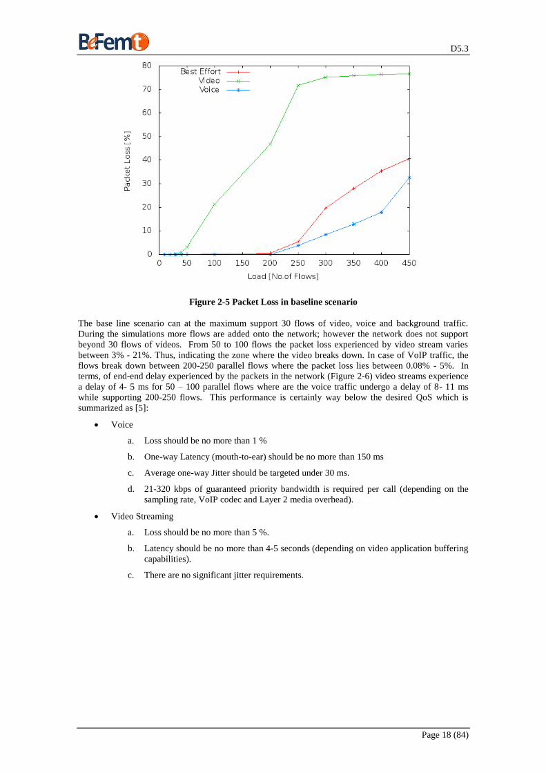
Figure 2-5 Packet Loss in baseline scenario
The base line scenario can at the maximum support 30 flows of video, voice and background traffic.
During the simulations more flows are added onto the network; however the network does not support
beyond 30 flows of videos. From 50 to 100 flows the packet loss experienced by video stream varies
between 3% - 21%. Thus, indicating the zone where the video breaks down. In case of VoIP traffic, the
flows break down between 200-250 parallel flows where the packet loss lies between 0.08% - 5%. In
terms, of end-end delay experienced by the packets in the network (Figure 2-6) video streams experience
a delay of 4- 5 ms for 50 – 100 parallel flows where are the voice traffic undergo a delay of 8- 11 ms
while supporting 200-250 flows. This performance is certainly way below the desired QoS which is
summarized as [5]:
Voice
a. Loss should be no more than 1 %
b. One-way Latency (mouth-to-ear) should be no more than 150 ms
c. Average one-way Jitter should be targeted under 30 ms.
d. 21-320 kbps of guaranteed priority bandwidth is required per call (depending on the
sampling rate, VoIP codec and Layer 2 media overhead).
Video Streaming
a. Loss should be no more than 5 %.
b. Latency should be no more than 4-5 seconds (depending on video application buffering
capabilities).
c. There are no significant jitter requirements.
D5.3
Page 19 (84)
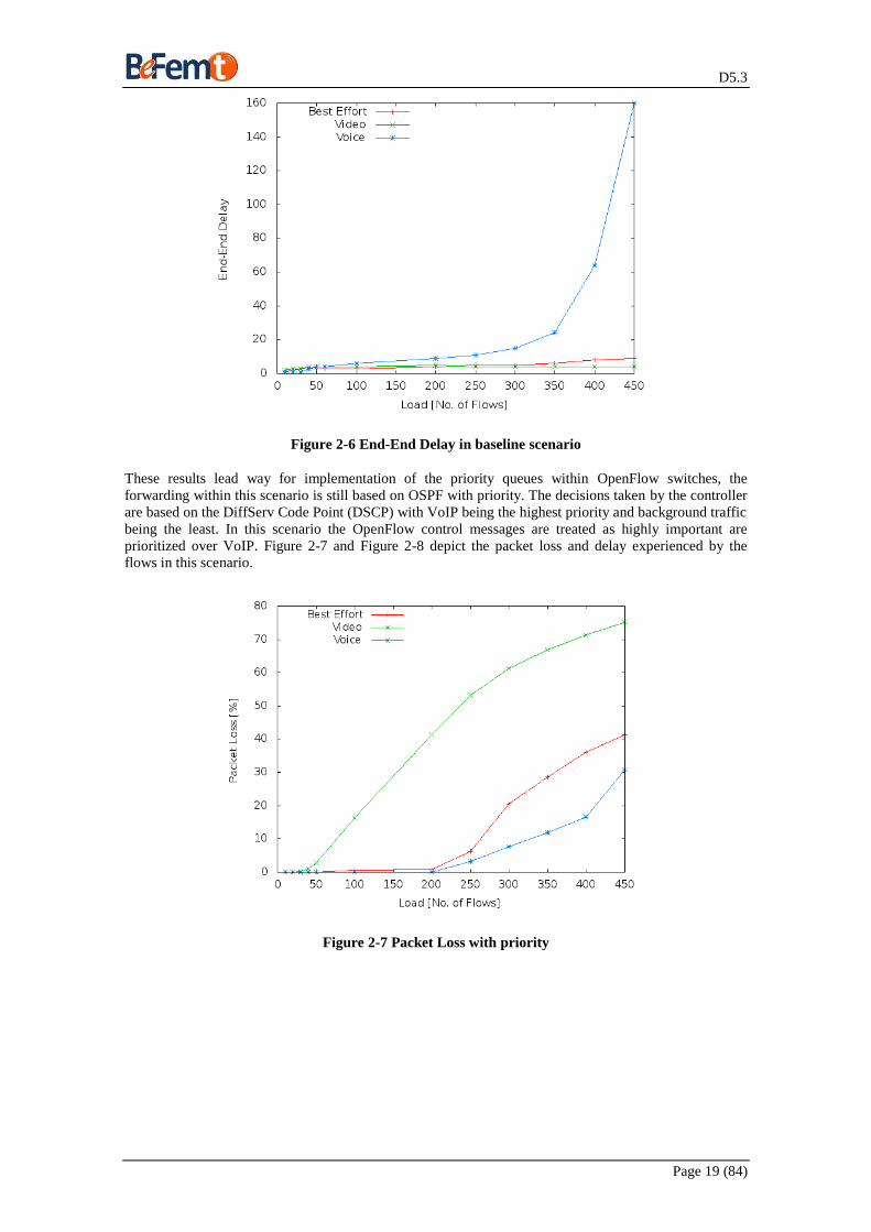
Figure 2-6 End-End Delay in baseline scenario
These results lead way for implementation of the priority queues within OpenFlow switches, the
forwarding within this scenario is still based on OSPF with priority. The decisions taken by the controller
are based on the DiffServ Code Point (DSCP) with VoIP being the highest priority and background traffic
being the least. In this scenario the OpenFlow control messages are treated as highly important are
prioritized over VoIP. Figure 2-7 and Figure 2-8 depict the packet loss and delay experienced by the
flows in this scenario.
Figure 2-7 Packet Loss with priority

D5.3
Page 20 (84)
Figure 2-8 End-End Delay with priority
The results show that the performance of the network is improved in this scenario. This was quite
expected because of the priority associated with the packet streams. The video stream experiences a
packet loss of 2%-16% (50-100 Flows) and for voice it varies from 0.05%- 3% (200-250 Flows). In terms
of delay the video streams range in between 2- 4 ms (50-100 Flows) and voice is placed between 3 – 4 ms
(200-250 Flows). Though the priority treatment improves the performance in terms of packet loss and
delays, these values are still below the expected QoS requirements. Moreover, they do not improve on the
number of flows which can be supported in parallel. This situation calls for implementation of more
advanced load balancing controllers which will not only assist in improving on the QoS within an
enterprise network but also result into more parallel flows in the network. This criterion is especially
important for the different stake holders in the enterprise femto network.
In the next section we introduce the well-studied valiant load balancing (VLB) technique [6] and analyse
its performance in an enterprise femto-network.
2.1.2.2 Evaluation of Load Balancing Network
VLB can be useful in an enterprise femto network because of the following desirable properties when
links fail or overload:
In order to protect against k failures the fraction of extra capacity required is only k/N, where N
is the diameter of the network. This is extremely efficient compared to other fault tolerance
schemes.
All of the working paths between a pair of nodes are used all the time, and flows are load-
balanced across all working paths. Most other schemes require protection paths that are idle
during normal operation.
VLB naturally protects against multiple failures. One can decide during design what failure
scenarios the network should tolerate, such as k arbitrary link or node failures or a particular set
of failure patterns.
All paths operate all the time, so rerouting is instantaneous
With these advantages, we implement the VLB controller in ns-3 environment with priority queues
discussed in the previous section.
D5.3
Page 21 (84)
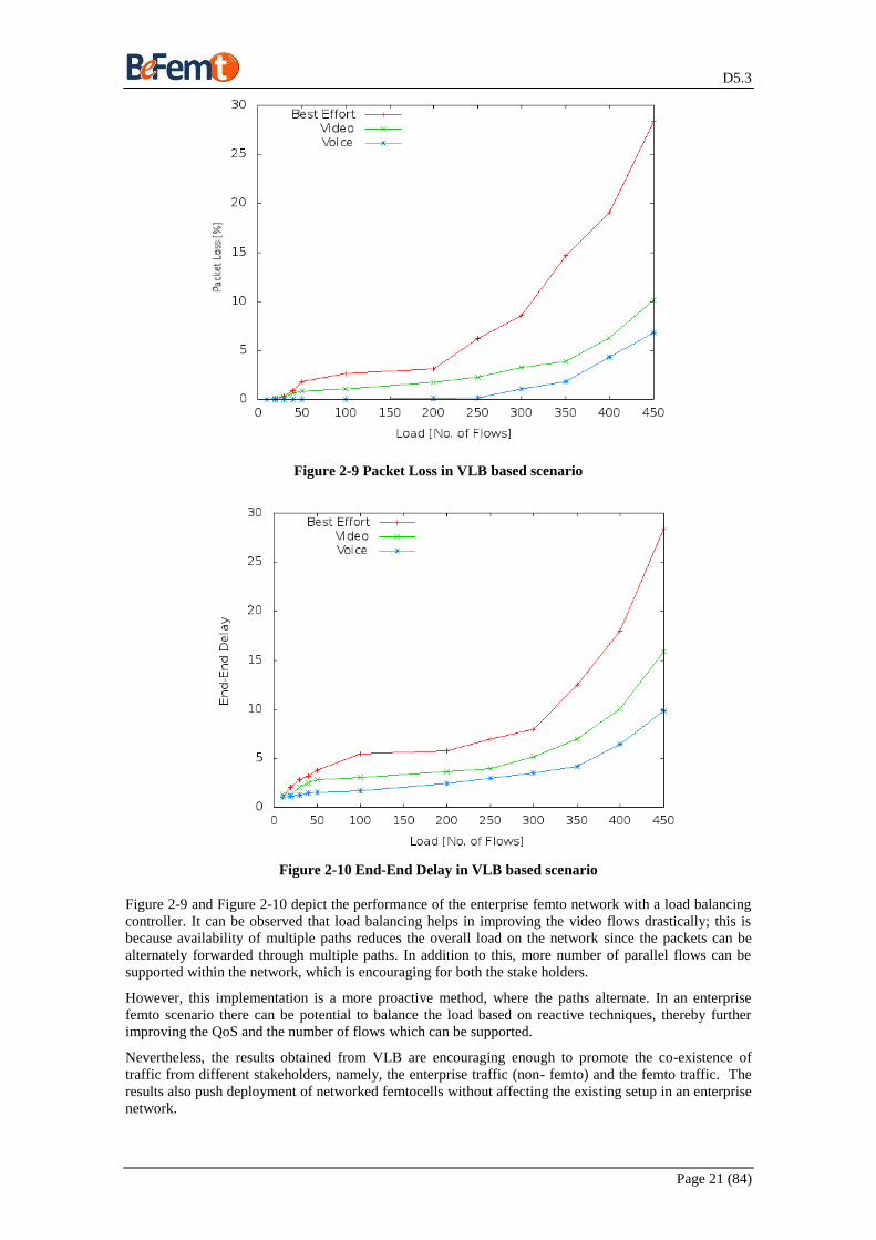
Figure 2-9 Packet Loss in VLB based scenario
Figure 2-10 End-End Delay in VLB based scenario
Figure 2-9 and Figure 2-10 depict the performance of the enterprise femto network with a load balancing
controller. It can be observed that load balancing helps in improving the video flows drastically; this is
because availability of multiple paths reduces the overall load on the network since the packets can be
alternately forwarded through multiple paths. In addition to this, more number of parallel flows can be
supported within the network, which is encouraging for both the stake holders.
However, this implementation is a more proactive method, where the paths alternate. In an enterprise
femto scenario there can be potential to balance the load based on reactive techniques, thereby further
improving the QoS and the number of flows which can be supported.
Nevertheless, the results obtained from VLB are encouraging enough to promote the co-existence of
traffic from different stakeholders, namely, the enterprise traffic (non- femto) and the femto traffic. The
results also push deployment of networked femtocells without affecting the existing setup in an enterprise
network.

D5.3
Page 22 (84)
2.1.3 Conclusion and Future work
The baseline scenario assisted in understanding the effects on the co-existing traffic. Here we found that
the video and voice traffic experience a significant degradation in QoS and very few parallel flows can be
supported. The analysis of second scenario, laid the foundation for understanding the overheads involved
in such cases and if traffic management can be achieved through a simple approach. The results show that
through priority queues the voice quality is significantly improved, however the video stream still
observed a degraded performance. This meant that there is a need for a better load balancing technique in
a cooperative femto network. The final scenario, facilitated to study the performance enhancement which
can be achieved for different stakeholders in a networked femto cell scenario using VLB method. VLB
when combined with OpenFlow switches can significantly improve the QoS for voice and video and also
support more parallel flows of traffic from different stakeholders. The performance enhancements
obtained from the load balancing scenario (OpenFlow with VLB controller) and further scope for
improvement results into key inference that, different stakeholders in a networked femto scenario need to
be supported by load balancing techniques to ensure the QoS. This can be ensured through the use of
OpenFlow switches which are connected to a centralized load balancing controller.
2.2 Distributed Routing
One important concern of any MNO is to minimize the cost of deploying infrastructure for the backhaul.
All-wireless network of femtocells (NoF) try to cover the necessity of giving cellular coverage in
scenarios where there is the need for a fast deployment and/or the deployment of fiber/copper would be
economically unfeasible (e.g., airports, shopping malls, temporary deployment in conference halls, or a
fixed deployment in a rural zone). As a result, MNOs have an increasing interest in the use of other
wireless technologies as backup technology, or even as primary backhaul due to the high cost and
unfeasibility of deploying wired infrastructure.
In this context, we conceived and developed a distributed routing protocol suited to such challenging
scenarios. If optimally tuned, this can entail several benefits for the MNO in terms of Operational
Expenditure (OPEX). Though the scheme designed can be used over any underlying wireless technology,
in this section we focus on studying the performance of Wi-Fi as a potential backhaul solution as a way of
evaluating the concept. Our target is to evaluate its feasibility and to give hints on under what conditions
(number of nodes, traffic load, number of gateways, etc.) these requirements may be fulfilled. Notice that
in this context, backhaul is understood as the wireless multi-hop network interconnecting the femtocells
that form the NoF, that is the local backhaul of the network of femtocells.
This section is organized as follows. In subsection 2.2.1, we summarize the work done during project year
2 on the extensive evaluation results of the distributed routing solution. After that, the final solution and
evaluation of the distributed routing solution enhanced with the variable-V algorithm is presented in
subsection 2.2.2. Subsection 2.2.3 presents the strategy taken for the deployment of multiple LFGW and
how the routing protocol benefits from this strategy without changes. Subsection 2.2.4 evaluates how the
proposed solution is able to circumvent holes in the NoF. Finally, subsection 2.2.5 draws conclusions.
2.2.1 Work during Year 2
The second project year consolidated the main ideas behind the distributed routing protocol proposed
during the first year (see D.5.2 [2] for a detailed explanation). Specifically, we studied the routing
problem from a Stochastic Network Optimization perspective exploiting Neely’s theoretical work [7].
Remarkably, to our knowledge this is the first practical study based on Neely’s Lyapunov optimization
framework for an all-wireless NoF. Moreover, we perform extensive simulation through ns-3 simulator
[8] of the resulting distributed backpressure routing protocol.
A summary of the main characteristics of the routing protocol shown in D5.2 follows. The resulting
distributed backpressure routing protocol is practical in the sense that, unlike previous theoretical
centralized algorithms [9], we presented a distributed implementation of the algorithm with low queue
complexity (i.e., one finite data queue at each node) to deal with any-to-any communications (i.e., uplink,
downlink and even local routing). In fact, we proposed a scalable and distributed routing policy that takes
control actions based on Lyapunov’s drift-plus-penalty minimization combining local queue backlog and
1-hop geographic information. Such framework offers a non-negative fixed parameter (V) for weighting
between both mentioned components.

D5.3
Page 23 (84)
A summary of the main evaluation work carried out with the routing protocol in D5.2 follows. We first
characterized its strengths and weaknesses against all-wireless NoF performance metrics such as
throughput, delay, and fairness injecting several flows. By means of ns-3 simulations under different
configuration setups, we studied the impact of the weight of the penalty function (i.e., the V parameter)
on the network performance metrics. In addition, we showed the influence of the location of the source-
destination pairs in these configuration setups. Finally, we evaluated the objective function-backlog trade-
off that characterizes Lyapunov optimization frameworks.
One of the most remarkable findings noted during the evaluation carried out in D5.2 is the existent trade-
off presented between 1) routing decisions for maintaining queue backlogs under control (and hence, the
all-wireless NoF stable) and 2) routing decisions trying to get close to the optimal value of an objective
performance metric. As a matter of fact, to achieve an appropriate trade-off the weight of the penalty
function denoted by the fixed parameter V is of primal importance.
The second finding is that fixed-V policies configured in every Home eNodeB (HeNB) cannot efficiently
handle NoF traffic dynamics in practical setups, since they will lead to queue overflows and/or
degradation of the objective metrics. We proposed the use of a practical distributed variable-V algorithm
that takes routing decisions aiming at achieving ideal objective metric values, yet not incurring into queue
overflows. An initial set of ideas to build this variable-V algorithm came out at the end of the second year
of the project.
Finally, we initiated the work towards the extension of the proposed distributed routing protocol to handle
multiple LFGWs, and the management of sparse deployments which are also subject of further study
during last half-year of the project.
In summary, along the next subsections, we provide a description of the work carried during the last half-
year of the project to continue the work towards the study of the previously mentioned open research
issues. Mainly:
In section 2.2.2 we show current progress, enhancements, and evaluation on the variable-V (or
adaptive weight) algorithm. Precisely, we come up with an additional variable-V algorithm
which provides several enhancements with respect to the previous variable-V algorithm defined
in D5.2.
Design, implementation, and evaluation of the distributed routing protocol to handle multiple
LFGWs leading to dynamic anycast backpressure routing in subsection 2.2.3.
Study of how the routing protocol behaves under sparse deployments with dead-ends in an all-
wireless NoF without changing its principles (i.e., stateless, distributed, self-organized, zero-
configuration in HeNBs, agnostic of the wireless backhaul technology) in subsection 2.2.4.
2.2.2 Variable-V algorithm: Final Solution and Evaluation
Results previously shown in D5.2 suggested the importance of a variable-V algorithm to avoid queue
drops at the NoF. Specifically, we showed that the traffic served could highly vary (in terms of
throughput, delay, jitter and fairness) depending on the V parameter. In an all-wireless NoF, it is expected
that the input rate matrix, and even the network topology could be variable in time. For instance, mobility
of UEs could also lead to changes in the input rate matrix in the NoF(i.e., the HeNB injecting traffic
coming from a given UE can change). On the other hand, HeNB in the network may fail tuning into an
inoperable state, hence changing the network topology. The distributed routing protocol enhanced with a
variable-V algorithm is able to react due to the adaptation to dynamic conditions the variable-V algorithm
poses. Furthermore, the fact that the variable-V algorithm is also distributed, and self-organized satisfies
the initial conditions posed by the all-wireless NoF (i.e., distributed, low-state…).
As explained in D5.2, the goal of the variable-V algorithm is to avoid queue drops while still minimizing
the penalty function (see D5.2 for a more detailed explanation of the routing algorithm). In D5.2 the
variable-V algorithm recomputed the V parameter for every HELLO message received from 1-hop HeNB
neighbours (i.e., on a per HELLO message basis). In next subsections, we provide more insights behind
this approach. Additionally, we propose two major changes in the calculation of the variable-V algorithm.
On the one hand, there is an additional algorithm that corrects the algorithm periodically calculated on a
per HELLO message basis per each data packet. On the other hand, there are some changes in the
computation of the variable-V algorithm on a per HELLO message basis.

D5.3
Page 24 (84)
2.2.2.1 Updates on the Variable-V algorithm calculation on a per HELLO messages basis
A description of the final variable-V algorithm updated from the algorithm described in D5.2 to
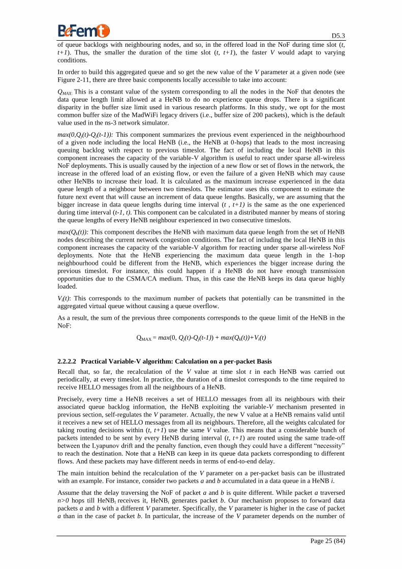
autoconfigure the V parameter in every HeNB follows. As depicted by Figure 2-11, a HeNB i builds a
virtual queue describing network conditions in terms of network load exploiting 0-hop (i.e, the info in the
current node), and 1-hop information of the data queues at every timeslot t. In other words, the variable-V
algorithm aggregates the information gathered from 1-hop HeNBs in terms of congestion to estimate
current, and future local network congestion conditions. To adjust Vi (t), the variable-V algorithm
estimates an upper bound of the expected maximum queue backlog in the 1-hop neighbourhood at time
slot t+1.
Specifically, the queue backlog has two components. First, a queue backlog quantifying congestion
around the 1-hop HeNB neighbourhood during current timeslot t. Second, a queue backlog estimating
future congestion at next timeslot t+1.
The goal of the variable-V algorithm is to increase the importance of the penalty function, while not
leading to queue drops in the data queues of the HeNBs. On the other hand, we showed in D5.2 that there
is a relation between the appropriate value of Vi(t) and the number of packet transmissions of node i. The
underlying idea behind our scheme lies in the fact that we consider Vi(t) as the maximum number of
packets that could potentially be greedily transmitted from node i to one of its neighbours j without
exceeding QMAX. In this case, greedily means that Lyapunov drift minimization is not taken into account
when sending traffic. This estimation is based on 1-hop queue backlog information at time slots t and t-1,
being t>0. More specifically, we propose the following distributed algorithm:
Figure 2-11 Illustration of the calculation of the variable value of V
Distributed Variable-V algorithm on a per HELLO message basis:
If t=0, Vi(t)=QMAX, at time t=1,2,3 … let
JjktQtQQQtV kjMAXMAXi ,)));(max)(max,max(,0max()(
where max(Qk (t)) is the maximum of all backlogs of nodes∈ J (i.e., the set of 1-hop neighbours of node
i), and max(∆Qj (t)) is the maximum differential Qj(t)-Qj(t − 1) experienced by 1-hop neighbour queues
of J between time slots t and t-1. The sum of max(Qk(t)) and max(0,Qj(t)-Qj(t-1)) provides an upper bound
(i.e., worst case) of the maximum queue backlog a neighbour of i may experience in time slot t+1,
assuming there is no sudden change neither in the offered load in the network nor in the topology. The
difference between QMAX and the estimated congestion at time slot t+1 in terms queue backlog
determines the value of Vi(t) for time slot t. Figure 2-11 is a representation of the worst case queue
backlog of the neighbor set of i expected at time slot t+1. Since the value of Vi(t) represents the maximum
number of allowed greedy transmissions from node i during a given time slot, Vi(t) is also a key
component in the estimation of the future more congested queue backlog in Figure 2-11.
1) Practical Considerations: The specific duration of the time slot determines the efficiency of the
proposed distributed routing algorithm. More specifically, the algorithm is assuming the knowledge of
past queue backlog differential information (i.e., Qj(t)-Qj(t-1)) to estimate future queue backlog
differentials. In other words, it is implicitly assuming that there are no abrupt changes in the differential
D5.3
Page 25 (84)
of queue backlogs with neighbouring nodes, and so, in the offered load in the NoF during time slot (t,
t+1). Thus, the smaller the duration of the time slot (t, t+1), the faster V would adapt to varying
conditions.
In order to build this aggregated queue and so get the new value of the V parameter at a given node (see
Figure 2-11, there are three basic components locally accessible to take into account:
QMAX: This is a constant value of the system corresponding to all the nodes in the NoF that denotes the
data queue length limit allowed at a HeNB to do no experience queue drops. There is a significant
disparity in the buffer size limit used in various research platforms. In this study, we opt for the most
common buffer size of the MadWiFi legacy drivers (i.e., buffer size of 200 packets), which is the default
value used in the ns-3 network simulator.
max(0,Qj(t)-Qj(t-1)): This component summarizes the previous event experienced in the neighbourhood
of a given node including the local HeNB (i.e., the HeNB at 0-hops) that leads to the most increasing
queuing backlog with respect to previous timeslot. The fact of including the local HeNB in this
component increases the capacity of the variable-V algorithm is useful to react under sparse all-wireless
NoF deployments. This is usually caused by the injection of a new flow or set of flows in the network, the
increase in the offered load of an existing flow, or even the failure of a given HeNB which may cause
other HeNBs to increase their load. It is calculated as the maximum increase experienced in the data
queue length of a neighbour between two timeslots. The estimator uses this component to estimate the
future next event that will cause an increment of data queue lengths. Basically, we are assuming that the
bigger increase in data queue lengths during time interval (t , t+1) is the same as the one experienced
during time interval (t-1, t). This component can be calculated in a distributed manner by means of storing
the queue lengths of every HeNB neighbour experienced in two consecutive timeslots.
max(Qk(t)): This component describes the HeNB with maximum data queue length from the set of HeNB
nodes describing the current network congestion conditions. The fact of including the local HeNB in this
component increases the capacity of the variable-V algorithm for reacting under sparse all-wireless NoF
deployments. Note that the HeNB experiencing the maximum data queue length in the 1-hop
neighbourhood could be different from the HeNB, which experiences the bigger increase during the
previous timeslot. For instance, this could happen if a HeNB do not have enough transmission
opportunities due to the CSMA/CA medium. Thus, in this case the HeNB keeps its data queue highly
loaded.
Vi(t): This corresponds to the maximum number of packets that potentially can be transmitted in the
aggregated virtual queue without causing a queue overflow.
As a result, the sum of the previous three components corresponds to the queue limit of the HeNB in the
NoF:
QMAX = max(0, Qj(t)-Qj(t-1)) + max(Qk(t))+Vi(t)
2.2.2.2 Practical Variable-V algorithm: Calculation on a per-packet Basis
Recall that, so far, the recalculation of the V value at time slot t in each HeNB was carried out
periodically, at every timeslot. In practice, the duration of a timeslot corresponds to the time required to
receive HELLO messages from all the neighbours of a HeNB.
Precisely, every time a HeNB receives a set of HELLO messages from all its neighbours with their
associated queue backlog information, the HeNB exploiting the variable-V mechanism presented in
previous section, self-regulates the V parameter. Actually, the new V value at a HeNB remains valid until
it receives a new set of HELLO messages from all its neighbours. Therefore, all the weights calculated for
taking routing decisions within (t, t+1) use the same V value. This means that a considerable bunch of
packets intended to be sent by every HeNB during interval (t, t+1) are routed using the same trade-off
between the Lyapunov drift and the penalty function, even though they could have a different “necessity”
to reach the destination. Note that a HeNB can keep in its queue data packets corresponding to different
flows. And these packets may have different needs in terms of end-to-end delay.
The main intuition behind the recalculation of the V parameter on a per-packet basis can be illustrated
with an example. For instance, consider two packets a and b accumulated in a data queue in a HeNB i.
Assume that the delay traversing the NoF of packet a and b is quite different. While packet a traversed
n>0 hops till HeNBi receives it, HeNBi generates packet b. Our mechanism proposes to forward data
packets a and b with a different V parameter. Specifically, the V parameter is higher in the case of packet
a than in the case of packet b. In particular, the increase of the V parameter depends on the number of
D5.3
Page 26 (84)
hops traversed by packet a. On the other hand, HeNBi uses the V parameter already calculated on a
HELLO message basis to forward data packet b.
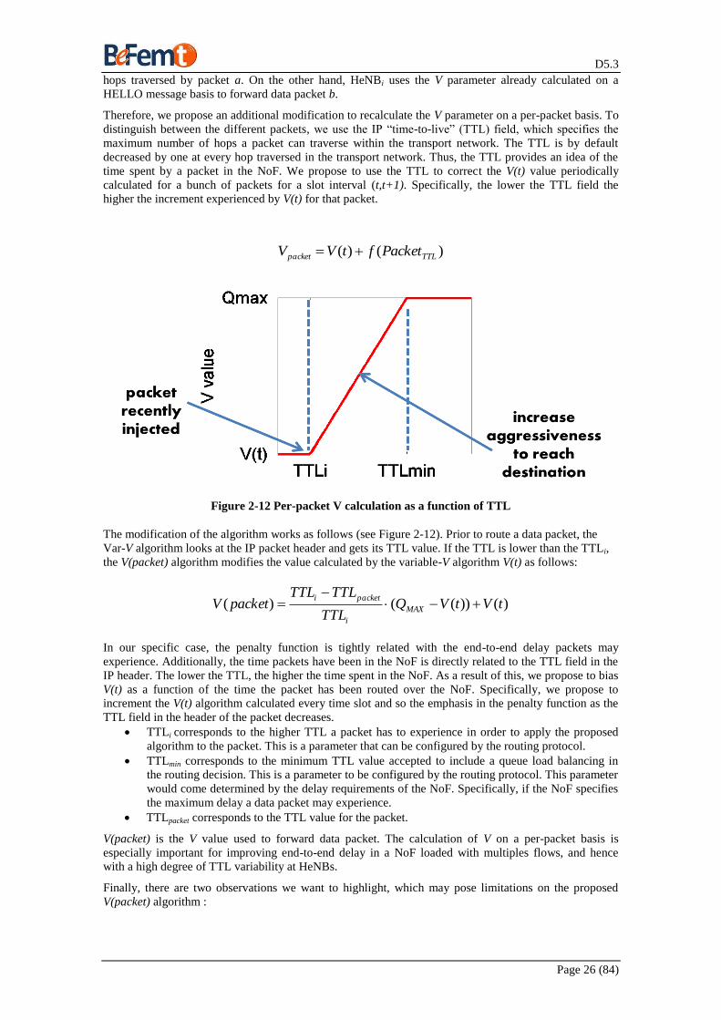
Therefore, we propose an additional modification to recalculate the V parameter on a per-packet basis. To
distinguish between the different packets, we use the IP “time-to-live” (TTL) field, which specifies the
maximum number of hops a packet can traverse within the transport network. The TTL is by default
decreased by one at every hop traversed in the transport network. Thus, the TTL provides an idea of the
time spent by a packet in the NoF. We propose to use the TTL to correct the V(t) value periodically
calculated for a bunch of packets for a slot interval (t,t+1). Specifically, the lower the TTL field the
higher the increment experienced by V(t) for that packet.
)()( TTLpacket PacketftVV
Figure 2-12 Per-packet V calculation as a function of TTL
The modification of the algorithm works as follows (see Figure 2-12). Prior to route a data packet, the
Var-V algorithm looks at the IP packet header and gets its TTL value. If the TTL is lower than the TTLi,
the V(packet) algorithm modifies the value calculated by the variable-V algorithm V(t) as follows:
)())(()( tVtVQTTL
TTLTTLpacketV MAX
i
packeti
In our specific case, the penalty function is tightly related with the end-to-end delay packets may
experience. Additionally, the time packets have been in the NoF is directly related to the TTL field in the
IP header. The lower the TTL, the higher the time spent in the NoF. As a result of this, we propose to bias
V(t) as a function of the time the packet has been routed over the NoF. Specifically, we propose to
increment the V(t) algorithm calculated every time slot and so the emphasis in the penalty function as the
TTL field in the header of the packet decreases.
TTLi corresponds to the higher TTL a packet has to experience in order to apply the proposed
algorithm to the packet. This is a parameter that can be configured by the routing protocol.
TTLmin corresponds to the minimum TTL value accepted to include a queue load balancing in
the routing decision. This is a parameter to be configured by the routing protocol. This parameter
would come determined by the delay requirements of the NoF. Specifically, if the NoF specifies
the maximum delay a data packet may experience.
TTLpacket corresponds to the TTL value for the packet.
V(packet) is the V value used to forward data packet. The calculation of V on a per-packet basis is
especially important for improving end-to-end delay in a NoF loaded with multiples flows, and hence
with a high degree of TTL variability at HeNBs.
Finally, there are two observations we want to highlight, which may pose limitations on the proposed
V(packet) algorithm :

D5.3
Page 27 (84)
The first observation is that the total delay accumulated by a data packet in the NoF is not
merely quantified by the number of hops traversed by a data packet. In addition to the number of
hops traversed by a data packet in the NoF, a more precise V(packet) estimator should take into
account the time spent by packets in data queues. A more complete study should be the one
taking into account both queueing delay, and the number of hops traversed in the NoF. However,
as a first approximation we opt the study which already shows important benefits in terms of
delay, as will be shown in section 2.2.2.3.
The second observation is the increase of the packet dropping probability due to queue drops
with the increase proposed by the V(packet) algorithm. Under high congestion conditions, the
V(packet) algorithm can force to forward a data packet to a HeNB neighbour quite congested,
leading to queue drops. This is likely to happen in a circumstance in which the TTL of the
forwarded packet is quite low. We propose to configure the TTLmin to a value in which the more
important factor is to reach the intended destination than maintaining a degree of load balancing
such that there are no queue drops at the expense of incrementing the queue drops in the
network.
2.2.2.3 Practical Variable-V algorithm: Evaluation
Evaluation Methodology:
In all the experiments evaluating the variable-V algorithm, the injected traffic consists of unidirectional
UDP with maximum packet size (i.e., 1472 bytes) at a CBR generated by the ns-3 OnOff application. The
duration of each simulation is of 120 seconds. The data queue size limit assigned to the HeNBs is of 200
packets. Therefore, in this case, using a V parameter greater than or equal to 200 means using the shortest
path in terms of Euclidean distance to the destination. On the other hand, the lower the V parameter (i.e.,
from 200 up to 0), the bigger the degree of load balancing offered by the backpressure routing protocol.
The wireless link data rate used by all HeNBs in the backhaul is a fixed rate of 54Mbps.
We label the variable-V algorithm computing periodically the V parameter as VarPrev-V, and the
variable-V algorithm computing the V on a per-packet basis as Var-V.
With regards to the configuration of the variable-V algorithms, the VarPrev-V algorithm calculates V
every 100ms, and the Var-V computes the V parameter for each data packet. We configured the TTLi to
60 in Var-V so that the data packets can traverse at least 4 hops in the NoF without giving importance to
the calculation of V on a per-packet basis. Additionally, the TTLmin is configured to 50, meaning that if a
packet traverses 14 hops the queue backlogs are not taken into account to compute forwarding decisions.
In this case we consider the data packet requires to be received by the destination even at the expense of
being dropped by a data queue.
A special case: Bidirectional Symmetric Traffic:
Figure 2-13 Throughput and Packet Delivery Ratio for VarPrev-V and Var-V algorithms

D5.3
Page 28 (84)
Figure 2-14 Comparison of Delay and Packet Delay Distribution for VarPrev-V and Var-V
algorithms
This experiment already illustrates the potential improvement in the packet delay distribution in the NoF,
comparing NoF performance metrics with the variable-V algorithm recalculating the V parameter every
100ms (i.e., VarPrev-V), and Var-V which includes the correction on a per-packet basis.
The experiment is based on sending bidirectional traffic between two HeNBs in the transport network.
The minimum distance between both HeNBs is of 5 wireless hops.
In this case, Figure 2-13 shows that in terms of packet delivery ratio and throughput, both variable-V
algorithms do not experience significant differences. Specifically, there is a slight decrease with the Var-
V algorithm, since it drops certain packets with a low TTL, not dropped by VarPrev-V. On the other hand,
Figure 2-14 shows that there are substantial differences between both Variable-V algorithms, with that
calculating V as a function of TTL on a per-packet basis performing much better.
MultiFlow:
Data packets originated from different sources and directed towards different destinations can traverse on
its way same HeNBs. Thus, it is likely that a HeNB has data packets accumulated in its queue with
different TTL values.
Figure 2-15 Throughput vs. load/number of flows for VarPrev-V and Var-V algorithms
The packets accumulated at data queues experience variability in their TTL as the number of flows in the
NoF grows. Data packets in a data queue may belong to different flows. Therefore, it is likely to observe
a higher variance of TTLs in a HeNB since they may be originated from different sources, and directed
towards different destinations. It is in these usual cases (i.e., 5 flows in a NoF) when the variable-V
algorithm calculating the V parameter on a per-packet basis demonstrates its potential for improving NoF
metrics such as throughput, and delay. On the other hand, a periodical computation of the variable-V
algorithm merely based on local congestion cannot attain this type of improvements, since it does not
provide such a fine granularity calculating the V parameter.
The experiment consists of injecting several flows in the NoF crossing the same set of HeNBs towards
different directions. Figure 2-15 provides throughput results of both variable-V algorithms with the
increase of the number of flows in the NoF. We observe significant improvements from the injection of 5
flows with the computation of the V parameter on a per-packet basis (i.e., Var-V) compared to the
periodical computation of the V parameter (i.e., VarPrev-V). Figure 2-16 provides delay results of both
variable-V algorithms with the increase of the number of flows in the NoF, in which Var-V also gives
better results.
We observe that adjusting the V parameter on a per-packet basis (i.e., Var-V) determines significant gains
in terms of end-to-end delay as well as throughput with the increase of the number of flows injected in the
NoF.

D5.3
Page 29 (84)
Figure 2-16 End-to-end delay vs. load/number of flows for VarPrev-V and Var-V algorithms
In the case of end-to-end delay, we observe a huge reduction in the packet delay experienced by Var-V
(i.e., the variable-V recalculating the V on a per-packet basis) with respect to that in VarPrev-V routing
policy. On the other hand, the end-to-end delay experiences improvements in the point in which at least 5
flows load the NoF, and increases from this point as the number of injected flows grow. In fact, the
average delay is reduced by 2x (i.e., 1 second) with respect to VarPrev-V (i.e., the previous variable-V
algorithm) for the case in which 7, and 8 flows load the NoF.
In the case of throughput, there is a significant improvement, especially when there are a high number of
flows injected into the NoF. Throughput results are practically equivalent when there are not excessive
flows loading the NoF. Specifically, in Figure 2-15 throughput results for both algorithms are similar
when the NoF backhaul handles 1, 2, 3, and 4 flows. However, we start observing remarkable throughput
improvements which are close to the 20% when 5 flows are injected in the NoF. Moreover, the
throughput improvements increase up to a point of 30% in the case in which the NoF is loaded with 8
flows.
2.2.3 Multi Local Femto Gateway
The introduction of several LFGWs may potentially increase the feasibility region, that is, the set of all
possible rates and flows that can be appropriately handled by the network. In fact, the capacity of wireless
links of LFGW is a potential bottleneck, as it acts as interconnector of the HeNB with the core network.
As a result, as the number of LFGWs capable of pulling packets from the NoF grows, the feasibility
region might also potentially grow.
2.2.3.1 Idea behind Dynamic Anycast Backpressure Routing
So far, in the solution proposed we assumed there is only one LFGW in the all-wireless NoF. However,
there might be several LFGWs for large-scale deployments. In an all-wireless NoF with multiple LFGWs,
there are some critical issues to take into account:
LFGW placement: The problem of LFGW placement is of primal importance in a NoF. The
efficiency of the LFGW placement strategy to choose will highly depend on the traffic demands
in that NoF, and also on the way the distributed routing protocol propose to do LFGW load
balancing.
Number of LFGWs: The more LFGWs are placed in the NoF, the more chances NoF
performance metrics can be optimized.
The first issue to solve is how to deploy the LFGWs in the all-wireless NoF so that distributed
backpressure routing can exploit LFGW load balancing. We propose a specific LFGW deployment
suitable for both the constrained environment posed by the NoF, and for the characteristics of the
distributed routing protocol.
The LFGW deployment follows. We deploy a single LFGW in the centre of the NoF in geographic terms.
This LFGW is referred as the reference LFGW. The reference LFGW is the one whose geographic
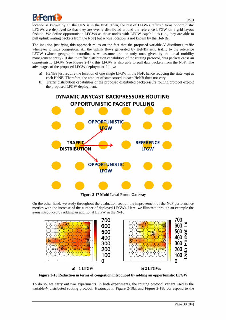
D5.3
Page 30 (84)
location is known by all the HeNBs in the NoF. Then, the rest of LFGWs referred to as opportunistic
LFGWs are deployed so that they are evenly distributed around the reference LFGW on a grid layout
fashion. We define opportunistic LFGWs as those nodes with LFGW capabilities (i.e., they are able to
pull uplink routing packets from the NoF) but whose location is not known by the HeNBs.
The intuition justifying this approach relies on the fact that the proposed variable-V distributes traffic
whenever it finds congestion. All the uplink flows generated by HeNBs send traffic to the reference
LFGW (whose geographic coordinates we assume are the only ones given by the local mobility
management entity). If due to traffic distribution capabilities of the routing protocol, data packets cross an
opportunistic LFGW (see Figure 2-17), this LFGW is also able to pull data packets from the NoF. The
advantages of the proposed LFGW deployment follow:
a) HeNBs just require the location of one single LFGW in the NoF, hence reducing the state kept at
each HeNB. Therefore, the amount of state stored in each HeNB does not vary.
b) Traffic distribution capabilities of the proposed distributed backpressure routing protocol exploit
the proposed LFGW deployment.
Figure 2-17 Multi Local Femto Gateway
On the other hand, we study throughout the evaluation section the improvement of the NoF performance
metrics with the increase of the number of deployed LFGWs. Here, we illustrate through an example the
gains introduced by adding an additional LFGW in the NoF.
a) 1 LFGW b) 2 LFGWs
Figure 2-18 Reduction in terms of congestion introduced by adding an opportunistic LFGW
To do so, we carry out two experiments. In both experiments, the routing protocol variant used is the
variable-V distributed routing protocol. Heatmaps in Figure 2-18a, and Figure 2-18b correspond to the

D5.3
Page 31 (84)
resulting data packet distribution injecting the same offered load to the NoF with 1 LFGW, and 2
LFGWs, respectively. Figure 2-18a, and Figure 2-18b plot the average number of data packets per second
transmitted by every HeNBs. Notice that this figure is only for illustration purposes and the LFGW is not
at the centre, as in the simulation results presented below.
The offered load for both heatmaps consists of six unidirectional UDP flows sent by six HeNBs labeled as
“S” towards the LFGWs labeled as “X” (i.e., the reference LFGW).
The second heatmap illustrates the gains introduced by adding a second LFGW labeled as “X” (i.e.,
opportunistic LFGW) in the NoF. In particular, we observe a decrease of congestion in the transport
network since the amount of data packets per second transmitted by every HeNB is considerably reduced.
As can be shown in both figures, the predominant dark color in nodes transmitting packets in Figure
2-18a becomes lighter in Figure 2-18b due to the addition of an opportunistic LFGW close to the
reference LFGW. Therefore, the addition of a second LFGW close to the reference LFGW is considerably
relieving congestion in the NoF.
Since all HeNBs direct traffic to the reference LFGW, and the proposed variable-V distributed
backpressure routing protocol distributes traffic just when it finds congestion, an opportunistic LFGW
close to the reference LFGW can alleviate congestion in a high degree.
a)1 LFGW b) 2 LFGWs
Figure 2-19 Comparison between different routing variants (fixed-V and variable-V routing
policies) in terms of Aggregated Throughput with 1 LFGW and 2 LFGWs
Going back to the simulation results (i.e., reference LFGW at the centre of the NoF), Figure 2-19 plots the
gains experienced in terms of aggregated throughput by the addition of an opportunistic LFGW.
Furthermore, Figure 2-19 provides the comparison between different variants of the fixed-V routing
policy and the variable-V routing policy described in previous section.
We observe that fixed-V routing variants with low V values (i.e., V=0, V=50, and V=100) experience high
throughput gains by the addition of an opportunistic LFGW. Recall that, as extensively evaluated in D5.2,
low V values in a fixed-V routing policy imply a high degree of load balancing in the NoF. Therefore, for
low V values an opportunistic LFGW close to the reference LFGW is exploited since a considerable
amount of data packets are pulled by the opportunistic LFGW relieving congestion from the NoF. In
contrast, for high V values (i.e., V=150, V=200) the addition of an opportunistic LFGW does not lead to
such throughput gains as with low V values. This is consequence of the decrease in the use of the
opportunistic LFGW for pulling packets from the NoF. Recall that, as extensively evaluated in D5.2, the
increase of V in a fixed-V routing policy decreases the degree of load balancing in the NoF backhaul. As a
consequence, with high V values (i.e., V=150, V=200) it is less likely packets cross an opportunistic
LFGW given that the degree of load balancing is practically null.
On the other hand, the variable-V algorithm behaves similarly to the best fixed-V routing variant with 1
LFGW as well as with 2 LFGWs. Actually, the variable-V algorithm has the potential to adapt to both
previously described LFGW layouts without any additional knowledge by the HeNBs.
As will be shown in next subsection, in addition to the specific LFGWs layout, the traffic patterns are of
primal importance in order to determine the importance of the variable-V algorithm with respect to a
fixed-V routing policy. Additionally, the specific location of the reference LFGW influences in the
performance experienced by the fixed-V routing policy. In contrast, the variable-V routing policy
maintains its stability. With the variable-V algorithm it does not matter where we locate the reference
LFGW as long as the opportunistic LFGWs are not too far from the reference
one.

D5.3
Page 32 (84)
a) 1 LFGW b) 2 LFGWs
Figure 2-20 Comparison between different routing variants (i.e., fixed-V and variable-V routing
variants) in terms of End-to-end delay with 1 LFGW and 2 LFGWs.
1 LFGW b) 2 LFGWs
Figure 2-21 Comparison between different routing variants in terms of Packet Delivery Ratio
With regards to end-to-end delay results evaluation results show the following features. Note that when
evaluating end-to-end delay, as issue of primal importance is to take into account packet delivery ratio
results. For instance, with a single LFGW, the variable-V algorithm experiences higher delay results than
with some fixed-V policies such as V=100, V=150, and V=200. Nevertheless, in Figure 2-21 we observe
that with the variable-V algorithm close to a 40% of more data packets arrive to the reference LFGW.
On the other hand, as can be shown in Figure 2-21, end-to-end delay decreases with the addition of an
opportunistic LFGW in a different degree for all the routing variants under evaluation. The variable-V
routing policy is the one experiencing the higher decrease of end-to-end delay.
2.2.3.2 Multi LFGW Evaluation
Methodology:
The experiments are based on injecting a high offered load to the NoF. Specifically, there are 8 flows
injecting 6Mbps directed to one single LFGW (i.e., the reference LFGW). Moreover, we evaluate
different routing policies (i.e., fixed-V and variable-V). With regards to the number and location of the
LFGWs, we consider three different setups. In the first one, there is a single LFGW referred as the
reference LFGW located in the centre of the 10*10 node square grid NoF. The geographic location of the
reference LFGW is known by all the HeNBs in the NoF. The location of the reference LFGW is
equivalent along the three setups under evaluation.
In the second setup, there are two additional opportunistic LFGWs around the reference LFGW.
Specifically, the two opportunistic LFGWs are in the same row of the reference LFGW. In the third setup,
there are four additional opportunistic LFGWs around the reference LFGW.
For each experiment, the NoF selects 8 HeNBs to inject traffic directed towards the LFGW in the centre
of the grid. Furthermore, there might be also flows not directed to the LFGW in the centre but to another
HeNB (i.e., local routing). We do this in order to evaluate the Multi-LFGW solution in a more generic
traffic scenario. Specifically, there is a combination of uplink and local routing.

D5.3
Page 33 (84)
We measure the aggregated throughput attained by the LFGWs, the end-to-end delay attained in the
LFGW, and the packet delivery ratio during a time interval of 100 seconds. We repeat simulations 10
times choosing a different set of source HeNBs to inject traffic in the NoF. Varying the position of HeNB
sources 10 times provides a representative distribution of potential traffic sources in the grid NoF. All the
traffic coming from the HeNB sources close in Euclidean distance up to a case in which all source HeNBs
are evenly distributed in the NoF.
The evaluation compares the fixed-V, and the variable-V routing policies. Specifically, we choose as
fixed-V the following instances: V=0, V=50, V=100, V=150, and V=200. The variable-V routing policy is
the one computing the V parameter on a per-packet basis, explained in section 2.2.2.2.
Discussion of the Results:
The case of V=0 is very powerful in a many-to-one scenario but outside this case it experiences high
throughput degradation. This fact can be observed in the minimum throughput values attained by such
routing variant in Figure 2-22, Figure 2-23, and Figure 2-24. Those values correspond to a traffic pattern
in the NoF different than the many-to-one traffic scenario, hence becoming difficult to create decreasing
gradients towards the respective destinations.
Figure 2-22 Different routing variants (i.e., fixed-V and variable-V) in terms of aggregated
throughput with 1 LFGW
Figure 2-23 Different routing variants (i.e., fixed-V and variable-V) in terms of aggregated
throughput with 3 LFGWs

D5.3
Page 34 (84)
Figure 2-24 Different routing variants (i.e., fixed-V and variable-V) in terms of aggregated
throughput with 5 LFGWs
Figure 2-23 and Figure 2-24 show that all routing variants experience throughput gains with the addition
of opportunistic LFGWs with respect to throughput attained with a single LFGW (see Figure 2-22). On
the one hand, we observe that with the fixed-V routing policy, the degree of load balancing decreases with
the increase of the V parameter. The higher the V parameter the lower the chances data packets are pulled
from the network by an opportunistic LFGW.
In contrast, the variable-V routing policy attains the maximum throughput in average compared with
fixed-V routing policies.
As can be shown by throughput improvements observed in Figure 2-23 and Figure 2-24 with respect to
Figure 2-22, the distributed routing protocol uses opportunistic LFGWs even though the HeNBs injecting
traffic to the WiFi backhaul is not aware of the location of these opportunistic LFGWs. This is because
data packets can be delivered to any of the available LFGWs due to the enabled anycast routing
capabilities.
Variability increases with the number of LFGWs and minimum throughput attained increases with the
increase in the number of LFGWs for the variable-V routing policy. Figure 2-23 shows that in average the
offered load injected to the NoF is practically served with the Var-V routing policy.
High fixed-V policies (i.e., V=100, V=150, and V=200) exploit better the 3 LFGWs case than the 5
LFGWs case since in the 5 LFGWs layout, the opportunistic LFGWs are located physically slightly
farther from the reference LFGW. Therefore, for fixed-V routing variants, the more emphasis in V implies
a lower throughput gain with the addition of opportunistic LFGWs.
In the case of V=0, we observe that when the network scenario is merely composed by uplink traffic, the
throughput attained is the best from all routing variants including the variable-V routing policy. The main
issue with V=0 appears when the traffic is not only uplink but also local/downlink. In this case V=0
experiences a high throughput decrease. This is illustrated by minimum attained throughput values in
boxplots from figures Figure 2-22, Figure 2-23, and Figure 2-24. Remarkably, the Var-V routing policy
experiences the maximum values in terms of minimum aggregated throughput achieved at the LFGWs.
Figure 2-25 Different routing variants in terms of Delay 1 LFGW

D5.3
Page 35 (84)
Figure 2-26 Different routing variants in terms of PDR 1 LFGW
Figure 2-27 Different routing variants in terms of Delay 3 LFGWs
Figure 2-28 Different routing variants in terms of PDR 3LFGWs
Figure 2-29 Different routing variants in terms of Delay with 5 LFGWs
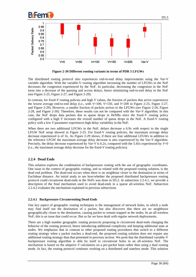
D5.3
Page 36 (84)
Figure 2-30 Different routing variants in terms of PDR 5 LFGWs
The distributed routing protocol also experiences end-to-end delay improvements using the Var-V
variable algorithm. With the variable-V routing algorithm increasing the number of LFGWs in the NoF
decreases the congestion experienced by the NoF. In particular, decreasing the congestion in the NoF
turns into a decrease of the queuing and access delays, hence minimizing end-to-end delay in the NoF
(see Figure 2-25, Figure 2-27, and Figure 2-29).
In contrast, for fixed-V routing policies and high V values, the fraction of packets that arrive experiences
the lowest average end-to-end delay (i.e., with V=100, V=150, and V=200 in Figure 2-25, Figure 2-27,
and Figure 2-29). However, a smaller fraction of packets arrives to the LFGWs (see Figure 2-26, Figure
2-28, and Figure 2-30). Therefore, these results can not be compared with the Var-V algorithm. In this
case, the NoF drops data packets due to queue drops in HeNBs since the fixed-V routing policy
configured with a high V increases the overall number of queue drops in the NoF. A fixed-V routing
policy with a low V parameter experiences high delay variability in the NoF.
When there are two additional LFGWs in the NoF, delays decrease a 6.9x with respect to the single
LFGW NoF setup showed in Figure 2-25. For fixed-V routing policies, the maximum average delay
decrease experienced is of 3x. As Figure 2-29 shows, if there are four additional LFGWs in addition to
the reference LFGW the maximum average delay decrease is also experienced by the Var-V algorithm.
Precisely, the delay decrease experienced by Var-V is 6.2x, compared with the 5.45x experienced by V=0
(i.e., the maximum average delay decrease for the fixed-V routing policies).
2.2.4 Dead Ends
This solution explores the combination of backpressure routing with the use of geographic coordinates.
One issue in the context of geographic routing, and so related with the proposed routing solution, is the
dead end problem. The dead-end occurs when there is no neighbour closer to the destination in terms of
Euclidean distance. An initial study to see how/whether the proposed distributed backpressure routing
protocol could circumvent dead-ends in the NoFs was done in D5.2. In subsection 2.2.4.1, we provide a
description of the final mechanism used to avoid dead-ends in a sparse all-wireless NoF. Subsection
2.2.4.2 evaluates the mechanism explained in previous subsections.
2.2.4.1 Backpressure Circumventing Dead-Ends
One key aspect of geographic routing techniques is the management of network holes, in which a node
may find itself not the destination of a packet, but also discovers that there are no neighbours
geographically closer to the destination, causing packet to remain trapped at the nodes. In an all-wireless
NoF, this is an issue that could occur. But so far we have dealt with regular network deployments.
There are a high number geographic routing protocols proposing to circumvent dead-ends changing the
behavior of the routing protocol, hence introducing additional complexity and keeping additional state at
nodes. We emphasize that in contrast to other proposed routing procedures that switch to a different
routing strategy when a packet reaches a dead-end, the proposed routing solution does not require any
additional routing strategy than that presented in previous section. We posit that the distributed variable-V
backpressure routing algorithm is able by itself to circumvent holes in an all-wireless NoF. The
mechanism is based on the adaptive V calculation on a per-packet basis rather than using a dual routing
mode. In fact, the routing protocol continues working on a distributed and stateless mode. This solution
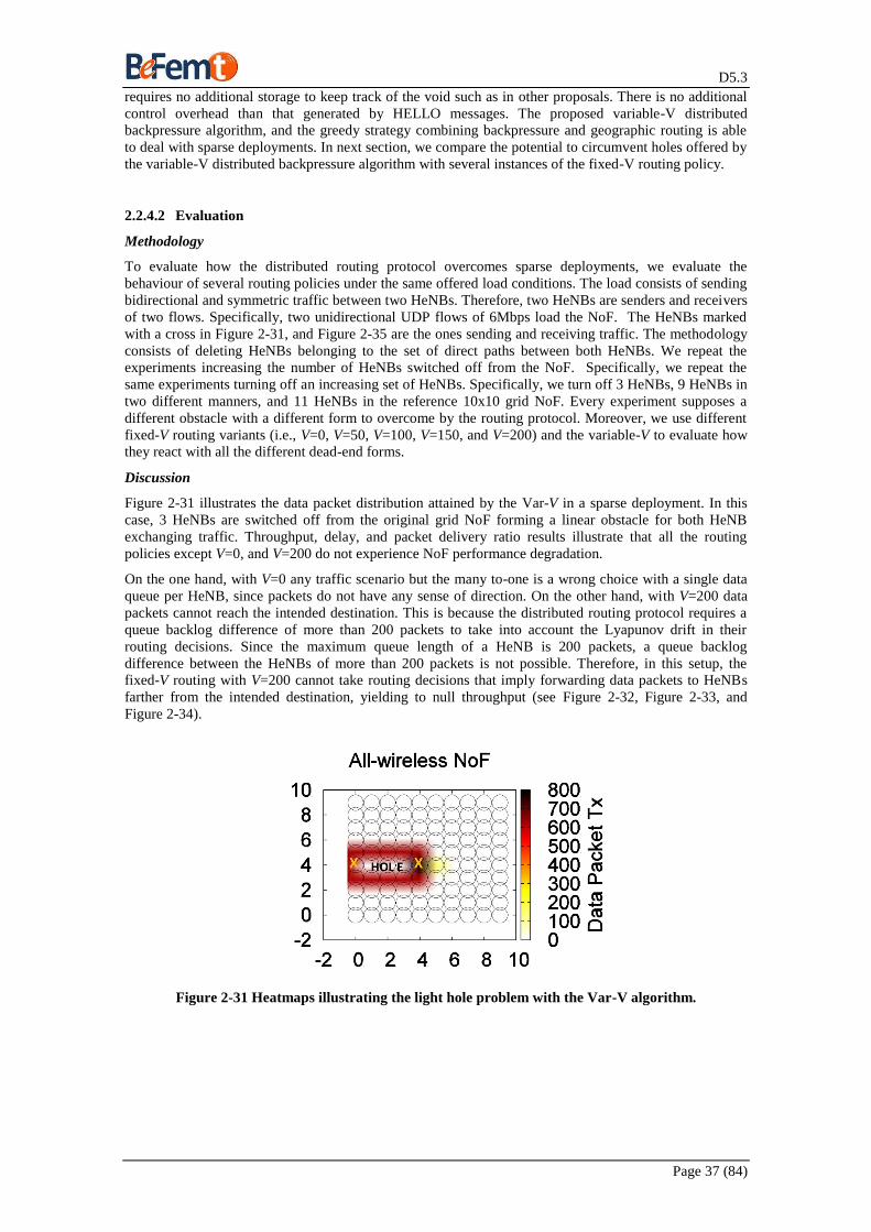
D5.3
Page 37 (84)
requires no additional storage to keep track of the void such as in other proposals. There is no additional
control overhead than that generated by HELLO messages. The proposed variable-V distributed
backpressure algorithm, and the greedy strategy combining backpressure and geographic routing is able
to deal with sparse deployments. In next section, we compare the potential to circumvent holes offered by
the variable-V distributed backpressure algorithm with several instances of the fixed-V routing policy.
2.2.4.2 Evaluation
Methodology
To evaluate how the distributed routing protocol overcomes sparse deployments, we evaluate the
behaviour of several routing policies under the same offered load conditions. The load consists of sending
bidirectional and symmetric traffic between two HeNBs. Therefore, two HeNBs are senders and receivers
of two flows. Specifically, two unidirectional UDP flows of 6Mbps load the NoF. The HeNBs marked
with a cross in Figure 2-31, and Figure 2-35 are the ones sending and receiving traffic. The methodology
consists of deleting HeNBs belonging to the set of direct paths between both HeNBs. We repeat the
experiments increasing the number of HeNBs switched off from the NoF. Specifically, we repeat the
same experiments turning off an increasing set of HeNBs. Specifically, we turn off 3 HeNBs, 9 HeNBs in
two different manners, and 11 HeNBs in the reference 10x10 grid NoF. Every experiment supposes a
different obstacle with a different form to overcome by the routing protocol. Moreover, we use different
fixed-V routing variants (i.e., V=0, V=50, V=100, V=150, and V=200) and the variable-V to evaluate how
they react with all the different dead-end forms.
Discussion
Figure 2-31 illustrates the data packet distribution attained by the Var-V in a sparse deployment. In this
case, 3 HeNBs are switched off from the original grid NoF forming a linear obstacle for both HeNB
exchanging traffic. Throughput, delay, and packet delivery ratio results illustrate that all the routing
policies except V=0, and V=200 do not experience NoF performance degradation.
On the one hand, with V=0 any traffic scenario but the many to-one is a wrong choice with a single data
queue per HeNB, since packets do not have any sense of direction. On the other hand, with V=200 data
packets cannot reach the intended destination. This is because the distributed routing protocol requires a
queue backlog difference of more than 200 packets to take into account the Lyapunov drift in their
routing decisions. Since the maximum queue length of a HeNB is 200 packets, a queue backlog
difference between the HeNBs of more than 200 packets is not possible. Therefore, in this setup, the
fixed-V routing with V=200 cannot take routing decisions that imply forwarding data packets to HeNBs
farther from the intended destination, yielding to null throughput (see Figure 2-32, Figure 2-33, and
Figure 2-34).
Figure 2-31 Heatmaps illustrating the light hole problem with the Var-V algorithm.

D5.3
Page 38 (84)
Figure 2-32 Attained throughput after switching off 3 HeNBs
Figure 2-33 Delay Distribution of Packets for routing variants able to circumvent the hole
Figure 2-34 Packet Delivery Ratio for routing variants able to circumvent the hole
a) Fixed-V V=100 b) Var-V
Figure 2-35 Illustration of the operation of Var-V and fixed-V algorithms in the presence of
obstacles
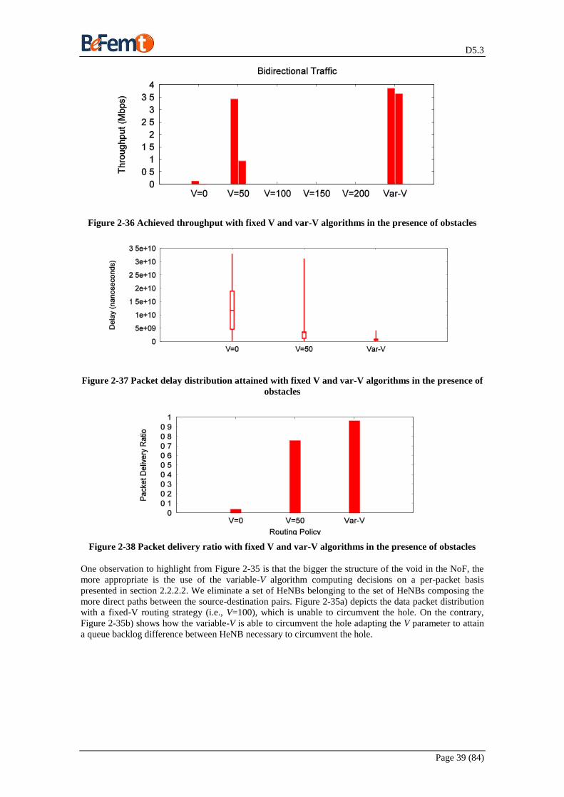
D5.3
Page 39 (84)
Figure 2-36 Achieved throughput with fixed V and var-V algorithms in the presence of obstacles
Figure 2-37 Packet delay distribution attained with fixed V and var-V algorithms in the presence of
obstacles
Figure 2-38 Packet delivery ratio with fixed V and var-V algorithms in the presence of obstacles
One observation to highlight from Figure 2-35 is that the bigger the structure of the void in the NoF, the
more appropriate is the use of the variable-V algorithm computing decisions on a per-packet basis
presented in section 2.2.2.2. We eliminate a set of HeNBs belonging to the set of HeNBs composing the
more direct paths between the source-destination pairs. Figure 2-35a) depicts the data packet distribution
with a fixed-V routing strategy (i.e., V=100), which is unable to circumvent the hole. On the contrary,
Figure 2-35b) shows how the variable-V is able to circumvent the hole adapting the V parameter to attain
a queue backlog difference between HeNB necessary to circumvent the hole.

D5.3
Page 40 (84)
Figure 2-39 Illustration of the operation of Var-V algorithm with complex obstacles
In fact, with V=100 the routing protocol requires a difference of 100 packets between neighbours to take
forwarding decisions that direct data packets farther from their intended destination. Since the maximum
queue size in a HeNB is of 200 packets, they cannot advance farther of the first hop in Figure 2-35a.
Therefore, the bigger the obstacle in the NoF, the lower the V parameter needed to overcome the hole.
The variable-V algorithm in every HeNB around the hole detects the accumulation of data packets, hence
reducing the V parameter and overcoming the obstacle. Packets in the perimeter of the hole eventually
reach the destination since HeNBs adapt their V so that a decreasing gradient is generated to reach the
destination on a per-packet basis. The potential of the variable-V algorithm can be shown in the results
obtained in terms throughput, delay, and packet delivery ratio. As can be shown in Figure 2-36, Figure
2-37, and Figure 2-38 there are only two routing configurations (i.e., fixed-V with V=50, and the variable-
V routing algorithm) able to circumvent the hole. However, the Var-V algorithm obtains the best results in
terms of throughput, delay, and packet delivery ratio.
The distributed routing protocol also shows its potential to circumvent complex holes such as the one
depicted in Figure 2-39. In this case, data packets have to circumvent a hole with a “U” shape. In this
unlikely sparse deployment in a NoF, the distributed backpressure routing protocol is also able to
circumvent the hole. The protocol in this case requires to direct data packets in the opposite direction of
the intended destination in order to circumvent the hole. It is able to achieve this by decreasing the V
parameter at HeNBs around the shadow of the hole. At the same time, these HeNBs accumulate data
packets at their queues, hence facilitating the decreasing queue backlog gradient towards the opposite
direction of the destination.
2.2.5 Conclusions
The proposed distributed variable-V algorithm seems a promising strategy in a constrained scenario an
all-wireless NoF poses. In particular, the routing protocol is able to obtain an interesting trade-off
between throughput and delay even under dynamic topologies, and traffic scenarios. Specifically, we
propose a variable-V algorithm that dynamically adapts the weight of Lyapunov drift-plus-penalty routing
decisions on a per-packet basis. The specific V parameter is function of the traffic load around the HeNB,
and the number of hops traversed by data packets. Furthermore, such weight (referred to as V) is
independently calculated at each node based on local queue backlog information, and it is easy to
implement. This variable-V algorithm aims at maximizing the relevance of the penalty function as much
as possible while avoiding queue overflows in the network. The evaluation results (with a simple penalty
function based on Euclidean Distance towards the destination) show an interesting trade-off between
throughput and delay. On the one hand, the throughput attained with the variable-V algorithm is similar to
the maximum throughput achieved with the best fixed-V algorithm. On the other hand, the proposed
variable-V routing policy outperforms all fixed routing setups in terms of delay, as it reduces delay
variation as well as the maximum delay. The proposed algorithm requires zero-configuration of the V
parameter, no matter the changes in the offered load to the network. Additionally, the variable-V
algorithm is agnostic of the particular penalty function used, since its calculation merely requires 1-hop
queue backlog information and data packet information.
D5.3
Page 41 (84)
We have extensively studied the distributed routing protocol under several circumstances comparing the
proposed variable-V algorithm with previous routing policies (fixed-V and variable-V routing policies).
The overall study indicates an interesting trade-off between throughput and delay, since it takes
forwarding decisions on a per-packet basis rather than on a periodical basis.
On the other hand, it has been shown to be appropriate in the multi-LFGW scenario, and to overcome
holes in sparse deployments. We proposed an easy way to deploy multiple LFGW in a NoF so that the
distributed backpressure routing protocol can exploit them without having knowledge of the location of
the opportunistic LFGWs. The main advantage observed is the decrease of congestion in the NoF with
respect to single LFGW NoF deployments, yielding to improvements in throughput, delay, and packet
delivery ratio. Finally, we evaluated the distributed routing protocol under several sparse deployments.
The study indicates the convenience of using the distributed routing protocol to circumvent holes
compared to fixed-V routing policies.
2.3 Traffic Offloading
2.3.1 Introduction
Nowadays there is enormous growth of the number of a new generation of mobile devices like various
smart phones (iPhone, Android-based), laptops, netbooks, etc. in the market. At the same time, mobile
networks operators are incorporating actively Internet applications and services for the mobile devices.
There are thousands of web data applications and services available now (e.g. YouTube, Facebook,
Spotify, IM, mobile TV, etc.) that are becoming extremely popular in the mobile user environment.
According to the Cisco VNI Global Mobile Data Traffic Forecast [10], overall mobile traffic is expected
double every year from 2011 onwards.
As a result of these two factors, there is an explosion of both data and signalling traffic towards the core
network of Mobile Network Operators (MNOs). As a consequence, congestion situations can arise in the
core network. Thus, solutions to avoid unnecessary traffic load at network nodes are needed. One such
solution is to apply a traffic offloading mechanism by means of femtocells. It can solve macro core
network capacity crunch avoiding future upgrades of the network infrastructure.
From a network management perspective it is very important to correctly understand performance
benefits (if any) of offloading in order to develop correct deployment strategies. Failing into doing so may
lead to investing large efforts in installing costly offloading infrastructures that do not bring targeted
benefits. In order to pursue these objectives it is important to characterize and model user behaviour and
data hotspots from the viewpoint of offloading strategy that MNOs plan to use. As a result, one must
assess if the gain in network resources obtained by means of traffic offloading is enough to avoid network
congestions.
Thus, the objective of this study is to analyse which are the benefits, coming from the deployment of an
offloading network in terms of performance.
In this study, we consider the traffic offloading process from the viewpoint of a MNO perspective. In this
context it is important for the MNO to care about a traffic load that goes to its core network (e.g. 3G CN)
after offloading. What is really needed for the MNO is to know what was before offloading and what
happens after in the context of traffic parameters to adjust with them dimensioning characteristics of its
network, e.g. to evaluate required system capacity after offloading.
Up to our knowledge, there has been no prior work analytically studying such offloading gains. An
eventual analytical framework is expected to help in taking network design decisions when deploying
offloading techniques. We make a contribution in this direction.
2.3.2 Work during Year 2
During the second project year, a model for the non-offloaded traffic of a single source that eventually
reaches the network of the operator has been proposed.
Based on previous measurements [11], we characterize the duration of offloading periods as heavy-tailed.
On the other hand, [12] and references therein present well-known models of the behaviour of single flow
traffic, which describe traffic burstiness in terms of long-range dependence and heavy-tails. In the same
way, we characterize user activity according to these models.

D5.3
Page 42 (84)
Thus, it assumes in our model that user activity periods Y(t) and periods characterizing offloading X(t)
are heavy-tailed. We model them as strictly alternating independent ON/OFF processes. Therefore, the
non-offloaded traffic Z(t) (i.e., that traffic still being served by the MNO on a regular basis) is modelled
as the product of these two processes Z(t) = X(t)Y (t) as shown in Figure 2-40.
Figure 2-40: Non-offloaded traffic from a single source (Z(t)) modelled as product of two strictly
alternating ON/OFF processes, X(t) and Y(t)
Operators are interested in the behaviour of the process modelling the aggregation of several Z(t)
processes. Therefore, our problem is to obtain an analytical model describing the behaviour of such an
aggregated traffic and the resource consumption it entails.
We have formed a high level view of the steps needed for solving the problem follows. Since, as
explained above, Z(t) has ON and OFF periods that follow heavy tailed durations, this process is long-
range dependent. Therefore, the aggregation of several such processes is self-similar and can be
characterized by means of the Hurst parameter (H). This can be done by means of the same techniques
presented in [13]. In turn, parameter H can be derived from the parameters characterizing the heavy-tailed
behaviour of the ON and OFF periods of Z(t). Besides, such parameters can be obtained from those of
processes of the original processes X(t) and Y(t). Therefore, once the parameters of the original processes
are known, by following the above steps, we can characterize the behaviour of the aggregated non-
offloaded traffic, and hence, the resources needed in the network of the MNO to serve it.
In this deliverable we present the main result of our research related to the main parameters characterizing
the asymptotic behaviour of the non-offloaded traffic, we validate the main results by means of
simulations, and we provide detailed analysis of performance evaluation issues related to resource
consumption in the network of the MNO deploying an offloading strategy.
2.3.3 Main Results
Lemma 1. Let Z(t) be the process resulting from the product of processes X(t) and Y (t). Let these two
latter processes have i.i.d. ON periods, i.i.d. OFF periods, and independent ON and OFF periods with
heavy-tailed distributions. The complementary distribution function for the ON-periods of process Z(t)
satisfies
where
and xon and
yon are the parameters characterizing the heavy-tails of the ON and OFF periods of
processes X(t) and Y (t), respectively. Hence, as α > 1,
Additionally, the complementary distribution function for the OFF-periods of process Z(t) satisfies
where

D5.3
Page 43 (84)
In (1), (4) cj > 0 is a constant and Lj(t)>0 is a slowly varying function at infinity.
Theorem 1. Let Z(t) be the process resulting from the product of two strictly alternating ON/OFF
processes X(t) and Y (t) with i.i.d. ON periods, i.i.d. OFF periods, and independent ON and OFF periods
with heavy-tailed distributions. Then, Z(t) is long-range dependent with covariance function:
where
Lemma 1 and Theorem 1 have been proved using proved using the probability theory laws and two
fundamental results related to this type of processes from [13][14].
2.3.3.1 Validation of main results
Taking into account the fact that both processes X(t) and Y (t) are heavy-tailed, we use the Pareto
distribution with parameters α and K (the scale parameter) to model both the ON- and OFF-durations of
the processes. In our simulations we use the Hill’s estimator [15] that provides a good way to estimate
tail-index α of Pareto-like tails [16]. In accordance with the methodology presented in [16], the ON- and
OFF-durations were simulated with 1010 states and 15000 largest sequences were considered out of them
in the estimation procedure. For a case study initial data were formed on a basis of statistical information
provided in the experimental studies on the performance of 3G mobile data offloading [13] (for the
process X(t)) and the burstiness of web traffic caused by accesses of HTTP clients to the heterogeneous
contents (text, images, PDF files, etc.) [17] (for the process Y (t)).
Thus, for the process X(t) we use the following initial data:
For the process Y (t) the input data are:
Figure 2-41: Estimation of the tail-index zmin by means of Hill’s estimator when
zmin=
zoff
In accordance with the simulations the tail-index of the process Z(t) is zmin1.1 as illustrated in Figure
2-41. This agrees with Theorem 1 according to which

D5.3
Page 44 (84)
In this case,
Figure 2-42: Estimation of the tail-index zon by means of Hill’s estimator
Figure 2-42 shows simulations to estimate the parameter zon, which in accordance with Lemma 1 should
be equal to 2.11 (x
on + y
on – 1). The result of the simulations matches well with the analytical result.
Figure 2-43: Estimation of the tail-index zon by means of Hill’s estimator when
zmin=
zon
The extensive simulations using Hill’s estimators were carried out for different sets of initial data and in
all cases values of the tail-index zmin were estimated correctly in accordance with the main results of the
analytical. As an example, for the data set x
on = 1.17, xoff = 1.8,
yon = 1.23,
yoff =1.55, we have a case
when in accordance with Theorem 1 zmin=
zon=1.4. As seen from Figure 2-43 it is perfectly agree with
the result of the simulations.
2.3.3.2 Performance bounds in offloading scenarios
We adopt the perspective taken in [18] and [19] in order to evaluate the system-wide implications of the
Lemma 1 and the Theorem 1. Specifically, we study which are the large-scale implications of
implementing an offloading strategy on the provisioning of resources in a mobile network.
In particular, Norros [19] derives an approximation of the capacity that a system requires under fractional
Brownian traffic in order to provide a target level of QoS, expressed as a bound (ε) on the amount of
traffic lost. Let us consider an arrival traffic model such as
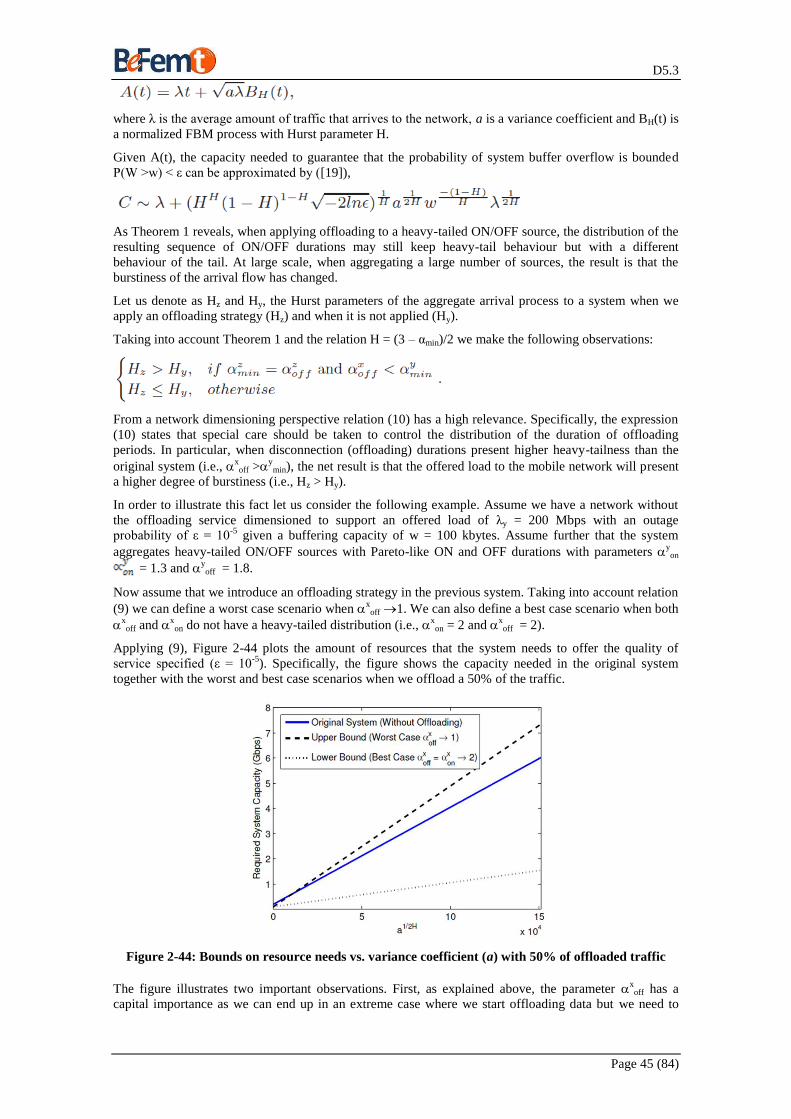
D5.3
Page 45 (84)
where λ is the average amount of traffic that arrives to the network, a is a variance coefficient and BH(t) is
a normalized FBM process with Hurst parameter H.
Given A(t), the capacity needed to guarantee that the probability of system buffer overflow is bounded
P(W >w) < ε can be approximated by ([19]),
As Theorem 1 reveals, when applying offloading to a heavy-tailed ON/OFF source, the distribution of the
resulting sequence of ON/OFF durations may still keep heavy-tail behaviour but with a different
behaviour of the tail. At large scale, when aggregating a large number of sources, the result is that the
burstiness of the arrival flow has changed.
Let us denote as Hz and Hy, the Hurst parameters of the aggregate arrival process to a system when we
apply an offloading strategy (Hz) and when it is not applied (Hy).
Taking into account Theorem 1 and the relation H = (3 – αmin)/2 we make the following observations:
From a network dimensioning perspective relation (10) has a high relevance. Specifically, the expression
(10) states that special care should be taken to control the distribution of the duration of offloading
periods. In particular, when disconnection (offloading) durations present higher heavy-tailness than the
original system (i.e., x
off >y
min), the net result is that the offered load to the mobile network will present
a higher degree of burstiness (i.e., Hz > Hy).
In order to illustrate this fact let us consider the following example. Assume we have a network without
the offloading service dimensioned to support an offered load of λy = 200 Mbps with an outage
probability of ε = 10-5
given a buffering capacity of w = 100 kbytes. Assume further that the system
aggregates heavy-tailed ON/OFF sources with Pareto-like ON and OFF durations with parameters yon
= 1.3 and yoff = 1.8.
Now assume that we introduce an offloading strategy in the previous system. Taking into account relation
(9) we can define a worst case scenario when xoff 1. We can also define a best case scenario when both
xoff and
xon do not have a heavy-tailed distribution (i.e.,
xon = 2 and
xoff = 2).
Applying (9), Figure 2-44 plots the amount of resources that the system needs to offer the quality of
service specified (ε = 10-5
). Specifically, the figure shows the capacity needed in the original system
together with the worst and best case scenarios when we offload a 50% of the traffic.
Figure 2-44: Bounds on resource needs vs. variance coefficient (a) with 50% of offloaded traffic
The figure illustrates two important observations. First, as explained above, the parameter xoff has a
capital importance as we can end up in an extreme case where we start offloading data but we need to

D5.3
Page 46 (84)
increase the amount of resources of the network to maintain a certain level of QoS (due to an increase of
data burstiness). Second, introducing a fine-grained control of the distribution of offloading periods can
be highly beneficial as it can also lead to decreasing the burstiness of data traffic to the core of the
network.
An alternative way to present this last observation is computing the amount of overprovisioning that the
system needs to keep up with a target QoS. In this context, overprovisioning is understood as the
resources beyond the average load that the operator must put in place to serve bursts of traffic. Figure
Figure 2-45 plots this for the same scenario as in the previous figure. In particular, it plots, for a fluid
model, the excess of resources over the total capacity that the network operator needs to implement to
maintain the objective probability of loss (ε). As the figure shows, in the worst case scenario even though
we reduce the amount of load to the system, we need to increase the overprovisioning margin to keep up
with the QoS. The contrary happens in the best case scenario where in addition to data traffic reduction
the operator can also relax overprovisioning needs.
Figure 2-45: Normalized overprovisioning of the system taking a fluid model approximation
Finally, let us consider Figure 2-46, which plots the relation Cz/Cy between the resources needed after and
before offloading with respect to the tail index of offloading periods (xoff). The figure illustrates the
influence of the different design parameters on the dimensioning of the network after applying offloading.
In particular, the figure focuses on illustrating the strong dependence of the effectiveness of offloading on
the actual distribution of offloading periods.
Figure 2-46: Illustration of the relation between the parameters of the system and the required
capacity before and after implementing offloading
Taking as a reference the dashed line in the figure indicating the amount of traffic offloaded (i.e., P(X(t)
is in ON state), it can be seen that when the distribution of offloading periods exhibits large tails (i.e., xoff
is low) there is a high probability that the network operator needs to increase resources to maintain QoS.
D5.3
Page 47 (84)
Another interesting observation is that the reduction on the number of resources is best (and cannot do
better than) when ),min( z
on
y
off
x
off .
As a summary, these facts illustrate that the main consequence of Theorem 1 is that the distribution of
offloading periods turns out to be the main design parameter in order to implement effective offloading
strategies in mobile network.
2.3.4 Conclusion
Operators are interested in benefits (if any) that traffic offloading implemented by means of femtocell
deployments can give for its network in terms of resource consumption. We proposed a theoretical
framework for studying mobile traffic offloading, in which both user activity and offloading periods are
modelled by means of strictly alternating ON/OFF processes whose ON and OFF durations are
characterized by heavy-tailed distributions. Furthermore, the process describing the non-offloaded traffic
(i.e., that traffic still needing to be served by the MNO on a regular basis) is modelled as the product of
the two previous processes. This framework is agnostic of the specific offloading technique applied as
well as the node where offloading is applied. We derived the exact parameters describing the asymptotic
behaviour of the non-offloaded traffic, which is shown to be long-range dependent with ON/OFF
durations following a heavy-tailed distribution. We also obtained the parameters characterizing this
process as a function of those of the original processes. Based on the characteristics of the aggregated
non-offloaded traffic, we provided performance bounds of resource consumption in the network of the
MNO when deploying offloading strategies. Furthermore, we illustrated the influence of the different
design parameters on the dimensioning of the network before and after applying offloading. We
concluded that offloading does not always entail a gain in terms of network resources and that the
appropriate design of offloading periods is key in network dimensioning. We validated the analytical
results by means of simulations.

D5.3
Page 48 (84)
3. Mobility Management
Mobility management mechanisms to support seamless handover with minimal signalling cost and enable
efficient location management for femtocells are developed in this section. For topics already studied in
previous deliverables, a subsection presents a summary of the work done. Section 3.1 further develops the
concepts already studied in previous deliverables on local location management in networks of
femtocells. In particular, this section focuses on describing a scheme for minimizing the impact of paging
control traffic over an all-wireless local backhaul. Section 3.2 introduces a new mechanism for reducing
the impact in terms of packet loss and service disruption time when handing over between macrocells and
femtocells.
3.1 Local Location Management
3.1.1 Introduction
This section describes an integrated solution for Local Location Management (LLM) in the context of
large-scale, all-wireless networks of femtocells (NoFs).
Traditionally, Mobility Management has been classified into Handoff Management and Location
Management. The former focuses on the provision of session continuity for voice and data calls during a
handover between neighbouring cells. The latter provides the necessary mechanisms to update the
location of a User Equipment (UE) within the NoF, and to page a mobile terminal when a voice or data
call is to be established. Formally, LLM deals with the extension of Location Management challenges to
the specific context of large-scale, all-wireless NoFs.
Standard 3GPP Location Management mechanisms have been designed with macrocell scenarios in mind.
Therefore, their performance in large-scale NoFs is far from optimal due to the overhead generated by
frequent handovers and cell reselections. Thus, NoF scenarios require specific Location Management
mechanisms in order to track UEs efficiently whilst keeping location signalling traffic under control. This
applies to both Tracking Area Update (TAU) (i.e., updating the location of a UE in the NoF) and Paging
procedures (notifying a UE in idle mode that a voice or data call needs to be established).
In the context of large-scale, all-wireless networks of femtocells, LLM provides a mechanism that enables
network entities to map a subscriber’s identity to the address and location of the HeNB where the UE is
currently camped on. On the one hand, standard 3GPP identifiers (such as the International Mobile
Subscriber Identity (IMSI) and/or the Serving Temporary Mobile Subscriber Identity (S-TMSI)) are used
to identify users within the cellular network. On the other hand, the serving HeNB address varies as the
destination UE moves throughout the NoF. This address is used by the underlying transport network to
route packets towards the destination UE. In order to avoid interoperability problems with current HeNB-
GWs and signalling traffic overload of the Evolved Packet Core (EPC), LLM mechanisms should only
affect the network elements in the NoF (i.e., the local network) and not the network elements of the
Evolved Packet Core (EPC).
3.1.2 Work during Years 1 and 2
The work carried out during the first two years has focused mainly on the definition of a distributed LLM
scheme (along with its associated protocol architecture) that is capable of providing LLM functionalities
in the context of a large-scale, all-wireless NoF. The LLM scheme is based on VIMLOC [20], a
distributed, wireless mesh network-oriented location management mechanism in which location
information is distributed across all HeNBs in the network of femtocells.
In order to integrate native 3GPP location management procedures with VIMLOC, modifications to the
protocol architecture of HeNBs were needed. As a result of this, a 2.5 protocol layer (also referred to as
geosublayer) was inserted between the network and access layers. One of the main functions of the
geosublayer was to intercept all 3GPP control-plane location management messages in order to trigger the
corresponding VIMLOC procedures in the network of femtocells. This work is described in detail in [1].

D5.3
Page 49 (84)
MAC
RLC
PDCP
SCTP
S1AP/X2AP
UDP
GTP-U
PHY
Geo SubLayer
HeNB
LLMIP/IPSec
STCP
S1AP
UDP
GTP-U
LLM
L2
IP/IPsec
LFGW Management
Relay
STCP
S1AP
UDP
GTP-U
Relay
Geo SubLayer
IP/IPSec
RRC
L1
Local Femto GW
L2
L1
L2
L1
Figure 3-1: The 2.5 Layer (Geosublayer) in the LLM Protocol Architecture.
VIMLOC relies on native 3GPP user location mechanisms in order to determine the IP and geographic
addresses of the HeNB where the destination UE is currently camped on. In order to do so, 3GPP
Location Management mechanisms must be able to determine, with the granularity of a single femtocell,
the current location of the destination UE within the NoF. Since standard 3GPP mechanisms can only
determine the location of a UE with the granularity of a Tracking Area (TA), a first approach to the
problem of fine-grained user tracking could be to reduce the size of all TAs in the NoF to that of a single
femtocell. However, this solution is far from optimal, as it requires UEs to perform Tracking Area Update
procedures every time they reselect/handover between neighbouring femtocells.
In order to address this problem, we proposed a self-organized Tracking Area List (TAL) mechanism
built on top of the standard 3GPP TAU procedure. This was done to comply with 3GPP Technical
Specifications. First, the Proxy Mobility Management Entity (P-MME) monitors the arrival rate of TAU
Request messages from the UE in order to determine its mobility state. Secondly, the P-MME updates the
UE-specific TAL by increasing, keeping, or reducing the number of cells in the TAL according to the
mobility state and the paging arrival rate. Finally, the MME sends the new TAL to the UE in the TAU
Accept message.
The self-organized mechanism combines static and dynamic TAL management depending on the UE
mobility state. Thus, TALs are kept static until the location signalling traffic reaches a certain threshold.
Past this activation point, the P-MME enables dynamic TAL management in order to reduce the overall
location signalling traffic in the network.
A detailed description of the self-organized TAL mechanism, along with some analytical results, has been
presented in [21].
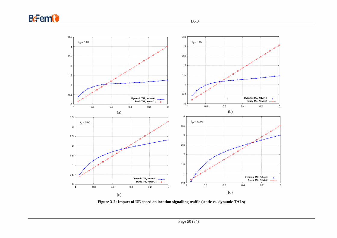
D5.3
Page 50 (84)
Dynamic TAL, Ndyn=4Static TAL, Nstat=2
(a)
Dynamic TAL, Ndyn=4Static TAL, Nstat=2
(b)
Dynamic TAL, Ndyn=4Static TAL, Nstat=2
(c)
Dynamic TAL, Ndyn=4Static TAL, Nstat=2
(d)
Figure 3-2: Impact of UE speed on location signalling traffic (static vs. dynamic TALs)

D5.3
Page 51 (84)
Figure 3-2 shows the impact of UE speed on the normalized signalling cost function for different paging
arrival rates (p). The normalized signalling cost function is a metric that captures both TAU and paging
signalling. In general, dynamic Tracking Area Lists generate less location signalling traffic than static
TALs for medium- to high-speed UEs. This reduction is significantly higher when UEs are subject to
moderate paging arrivals. Since the cost of a single TAU operation is tenfold that of a paging operation
[22], the self-organized TAL mechanism aims at minimizing the normalized signalling cost function by
reducing the probability of TAU arrival for each UE.
The intersections of the two curves in each figure determine the activation points of the self-organized
mechanism. Thus, at speeds where static TALs generate less location signalling traffic than dynamic
TALs, the self-organized mechanism keeps the TAL size constant. Once the activation point has been
reached, the P-MME enables dynamic TAL management, hence reducing the overall location signalling
traffic in the network. This switching strategy yields a significant reduction in location signalling traffic
per UE, as shown in Table 3-1.
p
Location signalling
traffic reduction
0.1 39.45%
1 33.53%
5 13.21%
10 4.45%
Table 3-1: Reduction in location signalling traffic per UE.
3.1.3 Enhancements to Proposed Schemes
One of the main drawbacks of the self-organized Tracking Area List mechanism is the cost (in terms of
signalling traffic) of paging a UE that has been registered to a large TAL (i.e., a UE in high-mobility
state). In the standard 3GPP Paging procedure, the (P)-MME sends an S1-AP Paging message (containing
the UE ID) to each cell in the TAL where the UE is currently registered. The impact of this scheme on
over-the-air signalling traffic is particularly relevant in large-scale, all-wireless NoFs.
In order to reduce the number of S1-AP Paging messages over the wireless multihop backbone, we
propose a distributed paging mechanism that structures the 3GPP Paging procedure in two stages. First, it
performs unicast paging from the P-MME to the closest HeNB in the destination TAL. Secondly, it
performs an efficient paging broadcast within the destination TAL by forwarding an optimal number of
Paging messages between neighbouring HeNBs over the X2 interface. This is described in details in the
sections below.
3.1.3.1 Description of the Distributed Paging Mechanism over the X2 Interface
The following sequence takes place during the execution of the distributed paging algorithm:
The P-MME receives a control-plane message from the MME (S1-AP Paging) or the P-SGW
(GTP-C Downlink Data Notification) indicating that an incoming voice/data call needs to be
established towards a certain UE in the NoF.
The P-MME looks up the destination UE ID (e.g., S-TMSI) in its internal location database and
determines the Tracking Area List ID where the UE is currently registered.
Once the destination TAL ID has been retrieved, the P-MME determines the closest HeNB (to
the P-MME) in the destination TAL. The P-MME stores the geographical location of each HeNB
in its internal location database. This information is obtained from the geosublayer at each HeNB
through O&M procedures.
The P-MME derives an optimal paging broadcast tree (in terms of number of over-the-air Paging
messages) for the destination TAL. The closest HeNB to the P-MME is the tree root.
The P-MME encapsulates the paging broadcast tree in the payload of an S1-AP Paging message
and sends it to the closest HeNB in the TAL. Note that a single S1-AP Paging message is sent
from the P-MME to the destination TAL over the all-wireless multihop backbone.

D5.3
Page 52 (84)
The closest HeNB to the P-MME in the TAL receives the S1-AP Paging message, performs a L1
paging procedure over the LTE-Uu interface, and sends an X2-AP Paging message to its one-
hop neighbours as per the information contained in the broadcast paging tree.
Upon receipt of an X2-AP Paging message, any HeNB in the destination TAL performs a L1
paging procedure over the LTE-Uu interface and sends an X2-AP Paging message to its one-hop
neighbours as per the information contained in the broadcast paging tree.
The destination UE is paged.
Figure 3-3 illustrates the operation of the standard paging and the distributed paging mechanisms in terms
of control-plane messages over the all-wireless multihop backbone.
UEUE
All-wireless multi-hop backbone
Destination Tracking Area
Destination UE
P-MME
S1-AP Paging
X2-AP Paging
LTE-Uu PagingUEUE
All-wireless multi-hop backbone
Destination Tracking Area
Destination UE
P-MME
Figure 3-3: Operation of the Standard vs. Distributed Paging Mechanisms
3.1.3.2 Implications in the 3GPP Protocol Architecture
The following implications in the 3GPP protocol architecture must be considered durign the design of the
distributed paging mechanism:
Geographic information availability at the P-MME: the P-MME must know the physical
location of each HeNB in the NoF in order to determine the closest femtocell in the destination
TAL. This information can be obtained from the geosublayer at each HeNB through O&M
procedures.
New Information Element (IE) in the S1-AP Paging message: an additional IE (PagingTree)
must be added to the structure of the S1-AP Paging message in order to encapsulate the optimal
paging broadcast tree for the destination TAL. The size of this IE must be kept bounded in order
to avoid large S1-AP Paging messages traversing the all-wireless multihop backbone.
New X2-AP Paging message: a new Paging message needs to be defined in the X2-AP
protocol. This message encapsulates the paging broadcast tree and is intended to allow Paging
notifications amongst neighbouring HeNBs.
The following tables summarize the modifications that need to be added to the corresponding 3GPP
Technical Specifications in order to provision the new S1-AP and X2-AP Paging messages.

D5.3
Page 53 (84)
Modifications to 3GPP TS 36.413: “Evolved Universal Terrestrial Radio Access Network (E-UTRAN); S1 Application Protocol (S1AP)”
Additions to the Technical Specification are highlighted in green.
9.1.6 S1-AP PAGING
This message is sent by the MME and is used to page a UE in one or several tracking areas.
Direction: MME eNB
IE/Group Name Presence Range IE type and reference Criticality Assigned Criticality
Message Type M 3GPP TS 36.423, 9.2.13 YES ignore
UE Identity Index value M 3GPP TS 36.413, 9.2.3.10 YES ignore
UE Paging Identity M 3GPP TS 36.413, 9.2.3.13 YES ignore
Paging DRX O 3GPP TS 36.413, 9.2.1.16 YES ignore
CN Domain M 3GPP TS 36.413, 9.2.3.22 YES ignore
List of TAIs 1 YES ignore
>TAI List Item 1 to <maxNoOfTAIs> EACH ignore
>>TAI M 3GPP TS 36.413, 9.2.3.16 -
CSG Id List 0..1 GLOBAL ignore
>CSG Id 1 to <maxNoOfCSGId> 3GPP TS 36.413, 9.2.1.62 -
Paging Broadcast Tree 0..1 YES ignore
>List of HeNBs 1 to <maxNoOfHeNBsInTree> EACH ignore
>> E-UTRAN Cell Identifier
M BIT STRING (28) -
Paging Priority O 3GPP TS 36.413, 9.2.1.78 YES ignore
Range bound Explanation
maxNoOfTAIs Maximum no. of TAIs. Value is 256.
maxNoOfCSGId Maximum no. of CSG Ids within the CSG Id List. Value is 256.
maxNoOfHeNBsInTree Maximum no. of HeNBs in the Paging Broadcast Tree. Value is 256.

D5.3
Page 54 (84)
Modifications to 3GPP TS 36.423: “Evolved Universal Terrestrial Radio Access Network (E-UTRAN); X2 application protocol (X2AP)”
Additions to the Technical Specification are highlighted in green.
9.1.2.23 X2-AP PAGING
This message is sent by the (H)eNB and is used to page a UE in one or several tracking areas.
Direction: (H)eNB (H)eNB
IE/Group Name Presence Range IE type and reference Criticality Assigned Criticality
Message Type1 M 3GPP TS 36.423, 9.2.13 YES ignore
UE Identity Index value M 3GPP TS 36.413, 9.2.3.10 YES ignore
UE Paging Identity M 3GPP TS 36.413, 9.2.3.13 YES ignore
Paging DRX O 3GPP TS 36.413, 9.2.1.16 YES ignore
CN Domain M 3GPP TS 36.413, 9.2.3.22 YES ignore
List of TAIs 1 YES ignore
>TAI List Item 1 to <maxNoOfTAIs> EACH ignore
>>TAI M 3GPP TS 36.413, 9.2.3.16 -
CSG Id List 0..1 GLOBAL ignore
>CSG Id 1 to <maxNoOfCSGId> 3GPP TS 36.413, 9.2.1.62 -
Paging Broadcast Tree 0..1 YES ignore
>List of HeNBs 1 to <maxNoOfHeNBsInTree> EACH ignore
>> E-UTRAN Cell Identifier
M BIT STRING (28) -
Paging Priority O 3GPP TS 36.413, 9.2.1.78 YES ignore
Range bound Explanation
maxNoOfTAIs Maximum no. of TAIs. Value is 256.
maxNoOfCSGId Maximum no. of CSG Ids within the CSG Id List. Value is 256.
maxNoOfHeNBsInTree Maximum no. of HeNBs in the Paging Broadcast Tree. Value is 256.
9.2.13 Message Type
The Message Type IE uniquely identifies the message being sent. It is mandatory for all messages.
1 As stated in 3GPP TS 36.423, section 9.2.13, the Procedure Code IE must be se to “16” (Paging).
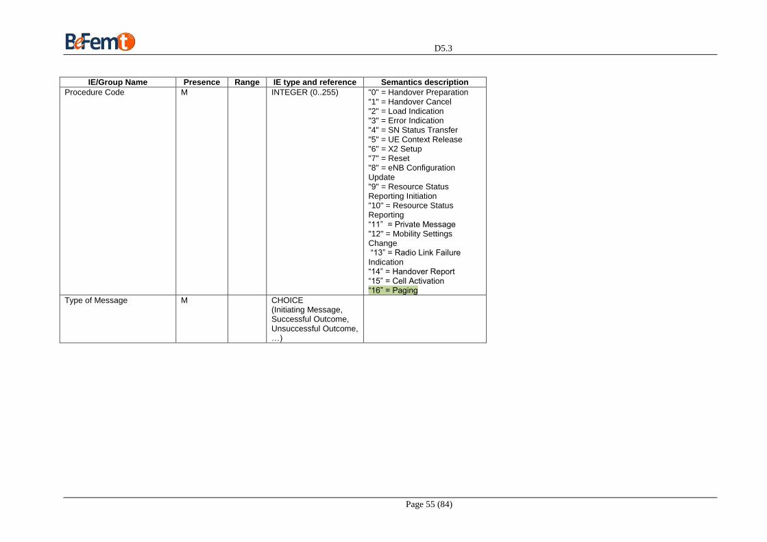
D5.3
Page 55 (84)
IE/Group Name Presence Range IE type and reference Semantics description
Procedure Code M INTEGER (0..255) "0" = Handover Preparation "1" = Handover Cancel "2" = Load Indication "3" = Error Indication "4" = SN Status Transfer "5" = UE Context Release "6" = X2 Setup "7" = Reset "8" = eNB Configuration Update "9" = Resource Status Reporting Initiation "10" = Resource Status Reporting “11” = Private Message "12" = Mobility Settings Change “13” = Radio Link Failure Indication “14” = Handover Report “15” = Cell Activation “16” = Paging
Type of Message M CHOICE (Initiating Message, Successful Outcome, Unsuccessful Outcome, …)

D5.3
Page 56 (84)
3.1.4 Performance Evaluation
Early results obtained with ns-3 show that the proposed scheme can achieve up to an 85% reduction of
over-the-air paging transmissions and an 80% of end-to-end paging delay reduction.
3.2 Seamless Macro-Femto Handover Based on Reactive Data Bicasting
3.2.1 Introduction
When a user moves from a macrocell to a femtocell or vice versa, seamless mobility should be supported
by the employed handover procedure such that the handover is not perceptible to the users. Two main
Key Performance Indicators (KPIs) during handover are Service Interruption Time (SIT) and packet loss.
In current 3GPP standard, the same hard handover procedure as for inter-macro mobility is used for
macro-femto mobility. A data forwarding procedure is used to forward the Downlink (DL) packets from
the source cell to the target cell during handover to enable lossless packet delivery. Whereas this
procedure works well for the handover between macrocells, it may be inappropriate for the handover
between macrocells and femtocells. In most deployment cases, the fixed broadband operators will have
no contractual agreements with the mobile network operators to provide guaranteed backhaul
performance. Thus, remarkable DL SIT up to several hundreds of milliseconds may be perceived by the
users in handover due to the data forwarding latency along the delay-prone residential backhaul.
Data bicasting or multicasting schemes have been widely used in literature to enable seamless handover
by pre-buffering the data at the potential target cells before handover. Conventionally, a candidate set of
the potential targets is dynamically updated based on the radio signal level and speed of a user. Duplicate
data is transmitted and buffered at all the cells in the candidate set [23][24]. However, given that the hard
handover is the only handover procedure supported by LTE so far, the maintenance of the candidate set
may require considerable modifications to the standard. Furthermore, the size of the candidate set may be
large due to the dense deployment of the femtocells. Proactively multicasting the data to all the cells in
the candidate set may consume numerous backhaul and buffer resources at these cells.
To enable seamless mobility while keeping minimal changes to the 3GPP standard, we propose a reactive
data bicasting scheme to reduce the DL service interruption time during HO by making “standard-
friendly” modifications to the 3GPP LTE HO procedure. Compared to the conventional schemes which
proactively trigger the data bicasting before the HO is initiated, the proposed scheme triggers the data
bicasting after the HO is initiated by the source cell. An optional drop-head buffering mechanism only
requiring a very small buffer size can be used at the S-GW to eliminate the packet loss during the HO
procedure. The proposed scheme can significantly relax the resource requirements compared to the
proactive data bicasting schemes.
3.2.2 Proposed Handover Procedure
A simple but effective modification based on the standard 3GPP HO procedure to enable seamless
handover when users move from a macrocell to a femtocell or vice verse is proposed. The modified
handover procedure is shown in Figure 3-4. When the MME receives the HO Required message from the
source cell, the MME will determine the target cell by checking this message and send a Data Bicasting
Request to the S-GW. When the S-GW receives this request, it will duplicate the downlink data packets
and bicast them to both the source and the target. The target cell maintains a receiving buffer for the
bicasted data. The other actions from the MME and the target cell are the same as the standard procedure
until the source cell receives the HO Command message.
Instead of sending the SN Status Transfer message to the target cell via the MME and forwarding the
downlink data to the target cell via the S-GW, the source cell will include the SN status in the RRC
Connection Reconfiguration message and send it to the UE. The data that arrives at the source cell after
the UE has been detached will be simply discarded. When the UE is synchronized with the target cell, the
UE will send the RRC Connection Reconfiguration Complete message with the SN status to the target
cell. Based on the SN status, the target cell can immediately determine the sequence number of the next
data packet to be transmitted to the UE and start both DL and UL data transmissions. The target cell then
sends the Path Switch Request including Bicasting Cancellation command to the MME. The MME will
send the UP Update Request to the S-GW to switch the downlink path from the source cell to the target
cell and at the same time cancel the bicasting. It is noted that most modifications can reuse the existing
messages defined in the standard. Therefore, the proposed scheme keeps minimal changes to the standard
procedure.

D5.3
Page 57 (84)
Figure 3-4: Proposed handover procedure
Since there is no data forwarding process from the source cell to the target cell during the HO, the data
packets will be lost if they arrive at the source after the UE is detached and are also not buffered at the
target. It will be shown in the following that the number of lost packets is very small. Actually, this loss
can be simply ignored for the real-time traffic such as VoIP. However, if lossless handover is required, an
optional drop-head buffering mechanism can be used to avoid the packet loss. Just before the HO, the UE
may send a Proximity Indication to the source cell if it determines that it is near a target cell. Note that the
proximity estimation method has already been proposed by 3GPP [25] to facilitate the HO to Closed
Subscriber Group (CSG) or hybrid cells. A Duplicating and Buffering Request will be sent by the source
cell and forwarded by the MME to the S-GW. A drop-head buffer with a size of N will be activated. Any
DL packet arriving at the S-GW will be duplicated before the original one is sent out. The duplicate copy
will be put into the drop-head buffer. The buffer will drop the packets from the front if it reaches its
maximum capacity, in other words, the buffer will always keep the latest N packets. When the S-GW
receives the Data Bicasting Request, it will first empty the drop-head buffer and send the packets in the
buffer to the target cell. A small buffer size will be enough to avoid the packet loss as will be shown in
the following.

D5.3
Page 58 (84)
3.2.3 KPI Analysis
In this section, the proposed handover procedure will be analyzed in terms of the two KPIs mentioned
before: expected DL service interruption time and expected number of lost packets. For the packet loss,
we analyze the case that there is no drop-head buffering at the S-GW. Thus, we can estimate the required
buffer size N if we want to avoid the packet loss during the HO. The similar analyzing methods can be
used for the handover from a macrocell to a femtocell and the handover from a femtocell to a macrocell.
In the following, we will take the former case for description purpose. The latencies incurred during the
handover procedure are denoted as follows:
: The transmission latency between the eNB and the MME.
: The transmission latency between the eNB and the S-GW. Without loss of generality, we
assume that and have the same distribution and can be denoted by the random
variable .
: The transmission latency between the HeNB and the MME.
: The transmission latency between the HeNB and the S-GW. Without loss of generality,
we assume that and have the same distribution and can be denoted by the
random variable .
: The HO execution latency from the time that the UE receives the RRC Connection
Reconfiguration message to the time that the target cell receives the RRC Connection
Reconfiguration Complete message. It can be denoted by the random variable .
The latency between the MME and the S-GW via S11 interface is very low (1 ms as stated in [26]). Thus,
we ignore this latency in the analysis.
We assume that , , and have mixed-Erlang density functions [27]:
where represents , , or . , , , and ¸ determines the shape and scale of the distribution
and . The mixed-Erlang distribution is selected here because it can achieve a good
approximation for many other distributions and real-world measurement traces [28]. Its corresponding
Laplace transform is given as:
3.2.3.1 Expected DL Service Interruption Time
For the 3GPP scheme, the data forwarding latency is , which can be represented by
the random variable with density function . The DL SIT is determined by the maximum
value between and . Note that the packet inter-arrival duration is not considered in the SIT since this
is not related to the handover procedure. Thus, the expected DL SIT can be derived as:
For the first term on the right side of the above equation, we have:

D5.3
Page 59 (84)
where is the Laplace transform of . Based on the convolution theorem, it can be denoted as:
For the second term on the right side, we have:
For the proposed scheme, if the buffer for storing bicasted data at the target cell is not empty when the
user gets connected, the communication session can be resumed immediately. Otherwise, the session will
be resumed when the bicasted packets arrive. When data bicasting is initiated at the S-GW, it takes
to arrive at the target cell. The duration from this moment to the time that the UE initiates the
detachment from the old cell and synchronization to the new cell is represented by the random variable
. The DL SIT is determined by the maximum value between and . and
have the same distribution as . Let with density function . Thus, the expected DL
SIT can be derived as:
D5.3
Page 60 (84)
There is no simple expression available for the solution of the above equation. The derivation process is
omitted here.
3.2.3.2 Expected Number of Lost Packets without Drop-Head Buffer at S-GW
Suppose that the S-GW receives the Data Bicasting Request message at time , the duration from this
moment to the time that the UE receives the HO Command message and is detached from the source is
represented by the random variable . The data packets will be lost if they have been sent to the
source before but arrived after the UE receives the HO Command message. It is assumed that the data
packets arrive at the S-GW according to a Poisson process with the arrival rate following the
assumption widely adopted in literature. Let denote the time at which the ith packet was sent from the
S-GW to the source cell tracking back from . has an Erlang distribution with the density
function:
Its corresponding Laplace transform is given as:
The transmission latency of the ith packet can be represented by the random variable that has the same
distribution as . Let denote the number of lost packets at the source cell during the HO procedure.
Let with density function . The expected number of lost packets is given as:
where is the Laplace transform of . Based on the convolution theorem, it can be denoted as:
3.2.4 Numerical Results
Numerical examples are evaluated in this section to investigate the two KPIs. Without loss of generality,
we use the setting and for , and , where represents , , or [27].
By referring to [29], we set ms and ms. For real-time applications such as VoIP and video
streaming, the packet inter-arrival time typically ranges from 10 to 40 ms. Thus, the packet arrival
rate ranges from 1/10 ms-1 to 1/40 ms-1.

D5.3
Page 61 (84)
(a) Expected downlink service interruption time (b) Expected number of lost packets without S-GW
buffering
Figure 3-5: Handover from macrocell to femtocell.
(a) Expected downlink service interruption time (b) Expected number of lost packets without S-GW
buffering
Figure 3-6: Handover from femtocell to macrocell.
Figure 3-5 and Figure 3-6 show the KPIs for the handover from macrocell to femtocell and from
femtocell to macrocell with respect to the expected femtocell backhaul latency, respectively. With the
increase of the femtocell backhaul latency, the expected DL SITs during both handovers will significantly
increase for the standard 3GPP handover procedure due to the data forwarding operation. On the contrast,
the proposed scheme only slightly increases the expected DL SIT for the handover from macrocell to
femtocell and keeps it almost constant for the handover from femtocell to macrocell. In the proposed
scheme, the DL data is bicasted to the target cell during the HO without requiring the data forwarding any
more. Therefore, the DL SIT is mainly determined by the inherent radio HO execution latency.
The expected number of lost packets when using the proposed scheme is negligible for the handover from
macrocell to femtocell. For the handover from femtocell to macrocell, it will increase as the femtocell
backhaul latency increases but still under 5 packets even when the femtocells backhaul latency is up to
150 ms. This implies that additional S-GW buffering mechanism is actually not necessary for the real-
time traffic such as VoIP where a small amount of lost packets are acceptable. In case that a lossless
handover is required, a small drop-head buffer at the S-GW will be enough to avoid the packet loss.
3.2.5 Conclusion
A novel handover procedure for LTE macro-femto networks based on reactive data bicasting is proposed.
The proposed scheme can significantly reduce the downlink service interruption time compared to the
standard 3GPP scheme while still avoiding the packet loss with the help of a small drop-head buffer at the
S-GW. The data will be bicasted to the source cell and the target cell only when the HO is actually

D5.3
Page 62 (84)
initiated, and thus, only a small receiving buffer is required at the target cell. The simplicity,
effectiveness, and limited resource requirements make it a promising solution to support seamless macro-
femto mobility.
D5.3
Page 63 (84)
4. Network Management
4.1 Energy Saving Network Management and Performance in HetNets
The current trend towards heterogeneous networks (HetNet), where a layer of macrocells for blanket
coverage co-exist with a layer of femtocells for providing capacity, will offer an improved spectral
efficiency per area, but it can also offer an opportunity to improve the energy efficiency, measured as the
power consumption needed to provide a certain throughput in a given area. We are going to analyze, two
network performance indicators, the aggregated throughput and the energy efficiency, in two network
architectures; a traditional deployment based on outdoor macro base stations for the provision of outdoor
and indoor coverage, which will be used as a benchmark scenario, and a deployment where some of the
indoor traffic is supported by femtocells.
Performance simulations and energy calculations have shown that the introduction of a femtocell layer,
complementing the macrocell layer, greatly improves the system performance and the energy efficiency,
when compared with current indoor coverage based on outdoor macro and micro base stations, even
though some procedures must be implemented to reduce the total power consumption of the femtocell
layer.
4.1.1 Current macro-only deployment limitations
Current mobile networks provide radio coverage by means of layers of base stations, based on a first layer
of high power macrocells, and a second layer of medium power microcells. In general these layers are
intended to provide simultaneous outdoor and indoor coverage, and thus are installed in outdoor
locations. This standard procedure has worked fine as long as the traffic has been mostly originated from
outdoors, but with the introduction of data-related services the scenario has reversed and the main traffic
demand comes now from indoors.
In this indoor traffic demand scenario, an approach where the coverage is provided from indoors becomes
preferable. The former solution incurs in high external walls penetration losses, and the latter is a natural
evolution of the cellular concept, reusing resources in ever smaller cells, and can make a better use of the
radio power as the femtonode and the user are located near each other, with minimal radio transmission
losses that translate in a higher spectral efficiency.
4.1.2 Macrocell coverage analysis from the energy efficiency point of view
Urban macro network deployments characteristics
The macrocell urban scenario is usually intended to provide a good outdoor coverage and a sufficient
indoor service, and its performance in dense urban deployments is usually interference-limited, because
the unwanted power from neighbouring cells becomes noticeable, as there is a high degree of overlapping
between small urban neighbouring macrocells. As a reference, 3GPP uses for a dense urban reference
scenario an inter site distance (ISD) of only 500 metres, and the average inter-site distance of currently
running networks in a dense urban scenario is around 200-300 metres.
LTE macrocell urban scenario simulation
A macrocell reference scenario with 18 LTE eNodeBs (54 cells) has been selected as an example of a real
urban deployment, where all the traffic is served with macrocells. This reference scenario is a dense urban
area in Madrid’s city centre (Salamanca district), with an area of 2.86 km2 and an average inter-site
distance of 250 metres.
The eNodeBs transmit a power of 46 dBm (40 watts) per sector, their operation frequency is 2.1 GHz,
their bandwidth is 10 MHz, and diversity is used in the eNodeB receivers. The overall capacity of this
scenario is calculated considering 10 active users per cell, i.e. 540 active users are randomly distributed
over the whole scenario, outdoor and indoor.
For the energy requirements analysis, the most favourable situation for the macro deployment has been
selected; assuming outdoor base stations that do not need any shelter or air conditioning, thus the
maximum consumed power per site, with three cells, is 790 W (based on actual eNodeB vendors’ data).
On the other hand, an eNodeB has always a minimum power level consumption, even when no traffic is
served, that is approximately a 40% of the full traffic load situation. In the intermediate traffic situations,
the power consumption is interpolated.
The macrocell reference scenario has been evaluated by means of a static radio planning tool (a
Telefónica’s proprietary tool) that calculates the signal level by means of a ray tracing tool core (Siradel)
using as an input a 3D cartography of Madrid’s city centre. Then the signal to noise ratio is calculated in a

D5.3
Page 64 (84)
grid of points in the reference scenario, and in a subsequent step the throughput in each point is calculated
using a LTE look up table (SINR – throughput). Finally the scenario’s average capacity is computed.
Macrocell scenario total throughput, total radiated power and total consumed power
The next figure shows the available throughput map. The aggregated average capacity for the 18 sites is
437 Mbps.
Figure 4-1. Available throughput map in the reference scenario
The total radiated power is 2,160 watts (40 watts/cell multiplied by 54 cells) and the total consumed
power is 14,220 watts (790 watts/site multiplied by 18 sites).
Macrocell scenario Figures of Merit
In order to give a clear insight of the energy efficiency of this scenario, we will use some figures of merit,
i.e. Mbps per watt, Mb/W. In the proposed reference scenario, when only the radiated power is
considered, Mb/W equals 0.203, and this value decreases to 0.031 when the total consumed power is
taken into account.
4.1.3 Combined macro and femto coverage analysis from the energy efficiency point of
view
Multilayer macro and femto urban scenario simulation
We are going to analyze the same geographical area described previously, but considering that a fraction
of the houses will install a femtonode. For this study it was used an 8 metre × 10 metre reference
apartment (see next figure), with brick exterior walls and plasterboard partitions, which is typical of
Madrid’s Salamanca district simulated area.
Figure 4-2. Reference 80 m2 apartment scenario with a central femtonode

D5.3
Page 65 (84)
In this scenario, the in-building area has a ground floor extension of 975,188 m2, and taking into account
that the average number of stories per building in the district is five; the total indoor area is 4,875,942 m2,
and there should be 60,949 reference apartments in this area.
The indoor section of the reference scenario has been evaluated by means of a Telefónica’s proprietary
indoor propagation tool based on COST 231 multi-wall model that characterizes indoor path losses by a
fix path loss exponent, plus additional path loss factors related with the empirical attenuation introduced
by all the walls crossed by the by the radio waves (considering the type of materials and their thickness).
It is assumed that femtocells and macrocells are using different frequencies; therefore there is not
significant interference between the macrocell and the femtocell layers.
In this exercise, 18% of the apartments, 10,971, have installed a femtocell. This 18% figure is one of the
femtocell penetration options that have been studied and selected as representative for a moderate
deployment scenario. Most of the apartments will enjoy a higher throughput than what could be provided
from a macro, improving the aggregated throughput in the reference scenario, and at the same time they
will offload the traffic and coverage requirements on the macro layer. For example, if an 18% of the
indoor area is served by femtonodes, the operator can afford to reduce every macro site power and
tolerate an indoor coverage gap (served from the macro layer) of the order of 18%. In our reference
scenario, the simulations performed indicate that macrocell radiated power per eNodeB can be reduced
from 46 dBm to 38 dBm (an equivalent result could be obtained reducing the number of sites), which
renders a macro site power consumption reduction from 790 W to 391 W.
Given this new reference scenario, the next step is to analyze the aggregated throughput and power
consumption. This exercise is deliberately pessimistic and therefore it is not considering femtocells
without interferences from neighbour femtocells, and thus most of the femtonodes are highly interfered.
The femtonodes are divided into four categories:
• Type 0 – Without an interferer femtocell. Not considered in this study.
• Type I –Serving Femtocell surrounded by one interferer femtocell, surrounded meaning that
there is a neighbour apartment where a femtocell is installed too. The simulation scenario sets that a 10%
of femtocells fall into this class (1,097).
• Type II – Serving Femtocell surrounded by two interferer femtocells. 40% of the scenario
femtocells are classified Type II (4,388).
• Type III – Serving Femtocell surrounded by five interferer femtocells. 50% of the femtocells are
considered to be Type III (5,486).
The percentages proposed for the distribution of the different types of femtonodes are an estimation,
based on the homes distribution in a densely populated area as Madrid’s Salamanca District. Every
femtocell is located at a height of 1 meter and radiates 15 dBm from a 6 dB gain omni directional
antenna. The consumed power per femtocell is 8 watts (data obtained from commercial 3G femtocells).
The operation frequency is 2.6 GHz and the bandwidth is 10 MHz.
The average cell throughput for each femtocell type is: 27.5 Mbps for Type 0, 19.1 Mbps for Type I, 17.9
Mbps for Type II and 17.5 Mbps for Type III.
There is not a noticeable performance degradation increase between Type II (two neighbour interferers)
and Type III (five interferers), because in Type III two of the interferers are located at the other side of a
corridor, separated with additional walls). This is the reason for not considering some intermediate
“Types”, for example a serving femtocell surrounded by 3 or 4 interfering femtocells. The next figure
shows the capacity results for a Type III femtocell.
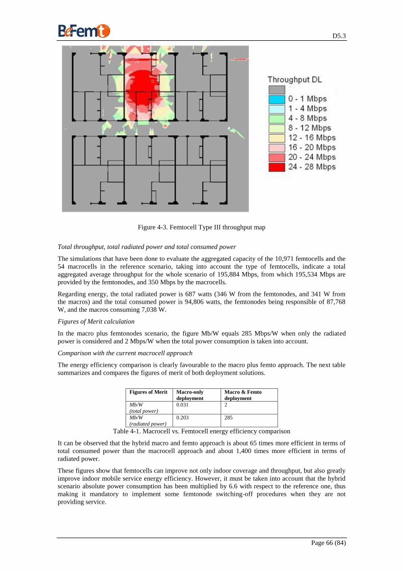
D5.3
Page 66 (84)
Figure 4-3. Femtocell Type III throughput map
Total throughput, total radiated power and total consumed power
The simulations that have been done to evaluate the aggregated capacity of the 10,971 femtocells and the
54 macrocells in the reference scenario, taking into account the type of femtocells, indicate a total
aggregated average throughput for the whole scenario of 195,884 Mbps, from which 195,534 Mbps are
provided by the femtonodes, and 350 Mbps by the macrocells.
Regarding energy, the total radiated power is 687 watts (346 W from the femtonodes, and 341 W from
the macros) and the total consumed power is 94,806 watts, the femtonodes being responsible of 87,768
W, and the macros consuming 7,038 W.
Figures of Merit calculation
In the macro plus femtonodes scenario, the figure Mb/W equals 285 Mbps/W when only the radiated
power is considered and 2 Mbps/W when the total power consumption is taken into account.
Comparison with the current macrocell approach
The energy efficiency comparison is clearly favourable to the macro plus femto approach. The next table
summarizes and compares the figures of merit of both deployment solutions.
Figures of Merit Macro-only
deployment
Macro & Femto
deployment
Mb/W
(total power)
0.031 2
Mb/W
(radiated power)
0.203 285
Table 4-1. Macrocell vs. Femtocell energy efficiency comparison
It can be observed that the hybrid macro and femto approach is about 65 times more efficient in terms of
total consumed power than the macrocell approach and about 1,400 times more efficient in terms of
radiated power.
These figures show that femtocells can improve not only indoor coverage and throughput, but also greatly
improve indoor mobile service energy efficiency. However, it must be taken into account that the hybrid
scenario absolute power consumption has been multiplied by 6.6 with respect to the reference one, thus
making it mandatory to implement some femtonode switching-off procedures when they are not
providing service.

D5.3
Page 67 (84)
4.1.4 Strategies to reduce energy consumption and interference in the femtonode layer
It must be taken into account that the femtonode users will not be at home during an important fraction of
the day, and then the femtonodes can be switched off, rendering a potential sharp reduction of the
aggregated power consumption described in the previous section, and also a reduction of the interference
generated by these femtonodes, at least that due to the control and broadcast channels which are always
transmitted regardless the presence of any UE.
Some implementations have been proposed for switching off the radio section of a femtonode when the
user is not in the neighbourhood of the femtonode. They detect when the UE is camped in the nearest
macro cell to the femtonode in order to decide when switching on or off the femtonode. When the User
Equipment is not camped in a predefined macrocell it is assumed to be far away from home and the
femtonode is switched off
The most efficient approach is to actually detect when the users are not at home, and thus switch off the
radio section of the femtonode, reducing interference and improving energy saving. A possible solution is
to detect the customer presence by means of a low-power radio interface activated in the UE, for example
a Bluetooth Low Energy, or Wi-Fi, which could be always active in the UE but whose low power
characteristic does not degrade significantly the battery lifetime. When the user arrives at home, a short
range radio connection between the UE and the femtonode is established, and the latter can switch-on its
radio section accordingly (the opposite is done when the user leaves the home and the short range
connection is lost). Currently, this strategy is under evaluation in 3GPP [30].
It must be taken into account that the standard cell reselection and handover procedures could not work
properly when the UE is moving from the coverage area of a macrocell to that of a femtocell whose radio
section has been switched off when no UE is camping in it, in particular when the femtocell switch on
procedure is performed only when the UE approaches to a very short distance of it. In the case the UE is
leaving the macrocell coverage and it is getting into the vicinity of the still switched off femtocell, the UE
will not have stored the femtocell cell RSRP among its reselection and handover candidate cells list.
When the UE is in idle mode, this will mean that there will be a period of time, from the moment it leaves
the coverage area of the macrocell, until it detects the RSRP of the femtocell once it has been switched
on, during which the UE will not be camping in any cell, and will be thus disconnected from the mobile
network.
On the other hand, when the UE is in connected state, the hand over procedure between the macrocell and
the femtocell could not be performed on time to keep the connection between the UE and the core
network active, because the UE will leave the coverage area of the macrocell and it will have to wait for
the femtocell to switch on, spend a certain period of time to measure its RSRP, and request to the MME
to start the handover procedure.
Some work has been done to improve the UE measurement process for cell reselection and handover
between standard LTE base stations that do not implement a radio section switch on/off procedure, for
example, dedicating more time and accuracy for the measurement of certain preferred base stations.
However, no work has been done to solve the specific problem of cell reselection and handover to a
femtocell whose radio section is off and thus the UE cannot measure any parameter of the target cell. This
is an open issue that will require further study.
D5.3
Page 68 (84)
5. Security
5.1 Local access control in networks of femtocells for multi-operator scenarios
5.1.1 Introduction
The scheme presented provides a solution to the problem of access control to local services in the NoF
(e.g., those offered to users visiting some company premises). The problem and also the solution are
divided into two different aspects: the access control part under the control of the mobile network
operator (MNO), and the access control to local services of the network of femtocells, which is under the
control of the local network operator (LNO) (e.g., the IT department of a company). The former is about
allowing UEs attaching to a femtocell that operates in the licensed spectrum of the MNO. The latter is
about providing a fine-granular control on what local services offered by the LNO can be accessed by
what UE and during what period of time.
Therefore, the LNO must have the ability to control which user equipments (UE) can have access to the
local network and to decide what resources it wants to share and which UE can use these resources. Given
the architecture defined in BeFEMTO for NoFs, the LFGW plays a key role in this respect, as explained
below. The standard mechanism used by BeFEMTO to share control between the MNO and the LNO is
the CSG [31]. In fact, both operators can control what UEs are allowed attaching to a given closed
subscriber group by appropriately managing the lists stored in core network servers in charge of
managing CSGs. When accessing CSGs, there are two scenarios to consider. In the first one the UE and
the femtocells in the NoF belong to the same HPLMN. The regular servers for CSG management (i.e.,
CSG Lists Server and CSG Admin Server) can be used in this case. This scenario was discussed in D5.2.
In the second one, when a roaming agreement is in place, the UE may access femtocells belonging to a
VPLMN. This is the focus of D5.3 in terms of access control.
In the multi-operator scenario, UEs from different MNOs are allowed to access local services offered by
the LNO. In this case, there is still the need for CSG membership management and two options exist,
namely HPLMN CSG Roaming (HCSG) and VPLMN Autonomous CSG Roaming (VCSG) [31].
VPLMN Autonomous CSG Roaming has been chosen instead of HPLMN CSG Roaming because of its
flexibility due to reduced administrative exchanges with the HPLMN. On the other hand, in case there is
the need for a fine-granular control by the HPLMN of what CSGs can be accessed by each UE in each
VPLMN, HPLMN CSG Roaming should be used instead [31], when supported. In fact, as stated in [32],
the following limitation appears when HCSG is used:
“The visited network needs to access the HSS/HLR in the home network of the subscriber in order to
update the CSG information for the subscriber. In some cases the visited network may not have access
to this function in the home network, for example, if the home network does not support CSGs when
the home network is Rel-7.”
This is the main reason why VCSG was introduced and it is still under discussion as of the time of writing
this deliverable. One way or the other, this allows that UEs that are not subscribers of the VPLMN have
access to CSGs defined by the VPLMN and jointly managed (through allowed and operator CSG lists) by
the MNO of the VPLMN and the LNO. However, since access to local services is a feature of interest to
the LNO, the VCSG approach offers a control as confined as possible in the LNO (and partially in the
VPLMN). In any case, the VPLMN must disable VCSG on a per HPLMN basis if so requested by the
home operator [31]. Therefore, home operators still keep the control of their UEs.
5.1.2 Work during Year 2
The main focus of the work on access control to local services during Year 2 was on single operator
scenarios in which the UE and the femtocells in the network of femtocells belong to the same Home
Public Land Mobile Network (HPLMN).
The same procedures as the ones presented below were studied in a single operator scenario, namely CSG
provisioning, access control enforcement at the MME based on CSG subscription information, and local
access control list provisioning. The message sequence chart of the interaction of the UE with local
services was also presented. In addition to that, the generic procedures for handling network security in
networks of femtocells were also studied.
The introduction of the CSG Subscription Server (CSS) in the work presented below allowed us to follow
the same general principles as those of year 2 for roaming UEs. However, some modifications are needed
for access control at the MNO level. On the other hand, access control at the local network level has been
simplified to allow for IT departments to apply their regular data networking access control policies also

D5.3
Page 69 (84)
for roaming UEs. Furthermore, in case the CSS is also used for UEs in the HPLMN of the femtocells, as
suggested in [33], the solution presented below would handle access control in a homogeneous manner
for both roaming and non-roaming UEs.
5.1.3 Relevant building blocks and interfaces
In addition to the building blocks mentioned in D5.2 for the single operator case, for the multi-operator
case, we exploit a new optional building block introduced in release 11 for storing CSG membership
information of roaming users: the CSG Subscription Server (CSS).
5.1.3.1 CSG Subscription Server (CSS)
According to TS 23.401 [34]: the “CSG Subscriber Server (CSS) is an optional element that stores CSG
subscription data for roaming subscribers. The CSS stores and provides VPLMN specific CSG
subscription information to the MME. The CSS is accessible from the MME via the S7a interface. The
CSS is always in the same PLMN as the current MME.” That is, the CSS performs the same function as
the HSS but only for handling CSG subscription data and procedures.
CSG Subscription information
According to TS 23.002 [35] and TS 23.008 [36], the CSS is responsible for holding the following user
related information:
User Identification;
CSG membership granted to the subscriber during his stay in the VPLMN, i.e. list of CSG IDs
and associated expiration dates; more specifically, TS 23.008 states that “If a mobile subscriber
has a Closed Subscriber Group (CSG) subscription, the HSS shall store Closed Subscriber Group
Information which is a list of up to 50 CSG-Ids per PLMN and for each CSG-Id optionally an
associated expiration date which indicates the point in time when the subscription to the CSG-Id
expires and optionally corresponding APNs which can be accessed via Local IP access from this
CSG identified by the CSG-Id”. In the same way, the CSS should also follow these rules.
User Location information: the CSS stores the location information of the subscriber for
subsequent update of the CSG subscription information at the MME upon subscription change.
The CSS consists of the following functionalities:
Download of the CSG subscription information upon request from the serving MME through the
S7a interface, to enable roaming subscribers to access to the packet switched domain services via
CSG cells;
Service provisioning, including updating the appropriate serving entities (i.e. MME) with
modifications of the CSG membership granted to the subscriber.
The interface between the MME and the CSS is S7a. There two main procedures defined through these
interface between these two entities, namely “insert CSG subscriber data” and “update CSG location” that
are initiated by the CSS and the MME, respectively. They are explained below in the context of CSG
provisioning and Access Control at the MNO level.
5.1.4 Relevant procedures
5.1.4.1 CSG provisioning
The procedure for adding, removing, or modifying the subscription of users is almost the same as that
presented in [37] except for the presence of the CSS. Therefore, in case the UE being registered does not
belong to the HPLMN, the administration server will contact the CSS instead of the HSS. The following
figure presents the message sequence chart for roaming UEs.

D5.3
Page 70 (84)
MMECSG
ManagerCSG ListServer
CSG AdminServer
CSS
Update CSG Membership{MSISDN, expiration_time}
Update CSG Membership{MSISDN, CSG_ID, expiration_time}
Update CSG Membership ACK
Update CSG Membership ACK
CSG update req
CSG update ACK
RoamingUE
Insert CSG Subscriber Data
Insert CSG Subscriber Data ACK
Update Allowed CSG list Request
Update Allowed CSG list Complete
Update Allowed CSG list over OMA-DM
Figure 5-1: CSG provisioning for roaming UEs involving the CSS
The LNO network manager (e.g., the system manager of the company) logs on to the administration
server and adds the new UE to the CSG that is already in place for providing access to local services to
guest UEs. The UE is identified by means of the MSISDN. If the modification is approved by the MNO,
the administration server then updates the CSS with the MSIDSN and CSG ID to which the UE is
allowed access. If the UE is currently attached to an MME, the CSS initiates the insert CSG subscriber
data procedure to modify the CSG information stored at the MME for this UE. This is done through the
S7a interface. After that, the CSS updates the allowed or operator CSG lists (depending on the operator
policy) in the CSG list server. Then, the CSG list server updates the UE with the new lists via OMA DM.
5.1.4.2 Access control at the MNO level
Once it has been registered, the UE is allowed to attach to femtocells belonging to a given CSG ID in the
visited network. Access control at the MNO level to control the attachment (and other NAS procedures)
to the appropriate CSG is described in the following figure. It is quite similar to that described in [37]
except for the presence of the CSS. The presence of the P-MME could be made transparent (however, see
the following subsection for some remarks on this).
UE HeNB LFGW MME CSS
NAS Request NAS Request UpdateCSG Location
Request
Update CSGLocation
AckNAS Accept
Figure 5-2: Access control at the MNO-level based on CSG subscription information retrieved from
the CSS
When the UE initiates a NAS procedure (e.g., attach, tracking area update), it is first sent to the HeNB
through an RRC message. The HeNB adds CSG related information to the message and sends the
corresponding S1-AP message towards the MME. If there is no subscriber information on the UE, the
MME will request it to the CSS as part of the roaming UE subscription profile in the form of an Update

D5.3
Page 71 (84)
CSG Location Request message. This will be ACK’ed by the CSS in the form of an Update CSG
Location ACK message. A prior interaction with the home HSS may be needed to retrieve roaming UE
subscription profile information. If the UE is not allowed to access this CSG, the MME sends a NAS
reject message with the cause value #25 (not authorized for this CSG). Otherwise, the MME sends the
NAS accept message.
5.1.4.3 Remarks on MNO-level operation
It is not needed that P-MME gets an update of subscriber information. This could still be handled by
MME in the core. However, if such update is feasible (i.e., allowed by MNOs via interfaces equivalent to
S6a or S7a), the operation would be more efficient, since access restrictions (if applicable) would be
applied closer to the UE, hence saving resources.
The procedures hitherto described handle the first part of the problem, that is, how does the MNO (of the
VPLMN or HPLMN), jointly with the LNO manager, grant access to a given CSG over licensed spectrum
of the MNO. Therefore, they allow the UE to initiate NAS procedures (e.g., attach, tracking area update,
service request) without being rejected.
The CSS only contains information on roaming UEs related with CSG management, all the rest of state
information (e.g., that stored in the HSS) and procedures (e.g., those related with other kind of subscriber
information exchange with the HSS) are not modified. Alternatively, one of the options mentioned in [33]
is that the CSS could also contain all CSG subscription information (that is, also for non-roaming UEs).
In this way, the HSS would not be overloaded with control information that is subject to temporary
subscriptions, and hence, potentially generating control information quite often.
5.1.4.4 Local Access Control List provisioning
On the other hand, the procedures described below solve the second part of the problem, that is, granting
access to the allowed local services.
In our solution, the MNO still has control on whether the roaming UE is allowed to have access to local
services through a “home APN”. In fact, it is expected that the MNO provides high-level offloading
policies only and the more fine-granular ones are fully under the control of the LNO. As explained in
D5.1 (section 2.2.4.2), the MNO could convey such policies by a TR069 management interface.
This control is enforced when the UE requests a PDN connection to the “home APN” that is received by
the MME, as part of the subscription information transferred by the HSS to the MME. On the other hand,
the fine-grained control of what services inside the local network are allowed to the roaming UE is under
the control of the LNO by applying regular data networking access control policies. This would allow
having homogeneous access control in the network of the company for all kinds of devices and
networking equipment (including mobile phones).
The main idea is that the LNO manager maintains a local AAA server with information on each roaming
UE indexed with its MSISDN. The allocated IP address for each UE is also stored in each record.
Therefore, the LGW will ask this server for the IP address to be assigned to the UE when it establishes the
PDN connection to the “home APN” [38]. As for access control lists, they could be manually configured
in the networking equipment of the company. Alternatively, there are schemes in which Access Control
Lists (ACLs) could also be stored for each UE in the local AAA in the form of downloadable ACLs. In
this case, when there is the first attempt from the UE to access a local service, the firewall would contact
the local AAA server for user authentication and for downloading the associated ACL if not already
enforced [39].
5.1.4.5 Remarks on LNO level operation
The LNO manager (e.g., the system manager of the company) configures the ACLs in the AAA server of
the LNO. Since ACLs will be applied based on fields of the IP data packet sent by the roaming UE (see
MSC of the next section), entries in the AAA server will contain MSISDN and IP address (as well as
expiration time). In this way, an appropriate mapping between the 3GPP identifiers and data networking
ones, in use in the local network, could be done. Notice that the roaming UE will be assigned an IP
address of the local network, which is fully under the control off the LNO manager.
The number of entities involved in the above MSC has been simplified by assuming that only the LNO
manager can grant access to roaming UEs. If any employee of the company could grant access to roaming
UEs, a new Local networked Femtocell ACL Administration Server entity (to which employees would
log on) could be introduced. In this way, the final approval before configuration in the AAA server would
still be given by the LNO operator.
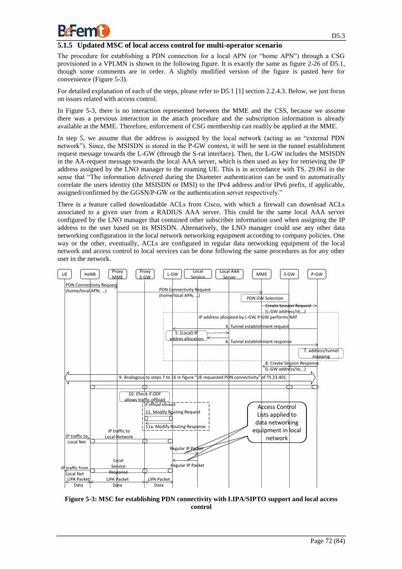
D5.3
Page 72 (84)
5.1.5 Updated MSC of local access control for multi-operator scenario
The procedure for establishing a PDN connection for a local APN (or “home APN”) through a CSG
provisioned in a VPLMN is shown in the following figure. It is exactly the same as figure 2-26 of D5.1,
though some comments are in order. A slightly modified version of the figure is pasted here for
convenience (Figure 5-3).
For detailed explanation of each of the steps, please refer to D5.1 [1] section 2.2.4.3. Below, we just focus
on issues related with access control.
In Figure 5-3, there is no interaction represented between the MME and the CSS, because we assume
there was a previous interaction in the attach procedure and the subscription information is already
available at the MME. Therefore, enforcement of CSG membership can readily be applied at the MME.
In step 5, we assume that the address is assigned by the local network (acting as an “external PDN
network”). Since, the MSISDN is stored in the P-GW context, it will be sent in the tunnel establishment
request message towards the L-GW (through the S-rat interface). Then, the L-GW includes the MSISDN
in the AA-request message towards the local AAA server, which is then used as key for retrieving the IP
address assigned by the LNO manager to the roaming UE. This is in accordance with TS. 29.061 in the
sense that “The information delivered during the Diameter authentication can be used to automatically
correlate the users identity (the MSISDN or IMSI) to the IPv4 address and/or IPv6 prefix, if applicable,
assigned/confirmed by the GGSN/P-GW or the authentication server respectively.”
There is a feature called downloadable ACLs from Cisco, with which a firewall can download ACLs
associated to a given user from a RADIUS AAA server. This could be the same local AAA server
configured by the LNO manager that contained other subscriber information used when assigning the IP
address to the user based on its MSISDN. Alternatively, the LNO manager could use any other data
networking configuration in the local network networking equipment according to company policies. One
way or the other, eventually, ACLs are configured in regular data networking equipment of the local
network and access control to local services can be done following the same procedures as for any other
user in the network.
UE HeNBProxy MME
Proxy S-GW
L-GW MME S-GW P-GWLocal AAA
Server
PDN Connectivity Request(home/local APN, …) PDN Connectivity Request
(home/local APN, …)PDN GW Selection
Create Session Request(L-GW address/id,…)
IP address allocated by L-GW, P-GW performs NAT
4. Tunnel establishment request
5. (Local) IPaddres allocation
6. Tunnel establishment response
7. address/tunnelmapping
8. Create Session Response(L-GW address/id,…)
9. Analogous to steps 7 to 16 in figure “UE requested PDN connectivity” of TS 23.401
IP traffic toLocal Net
LIPA PacketData
Regular IP Packet
Regular IP PacketIP traffic from
Local Net
Local Service
Response
Local Service
IP traffic toLocal Network
10. Check if ODF allows traffic offload
11. Modify Routing Request
11a. Modify Routing Response
LIPA PacketData
LIPA PacketData
If offload allowed Access Control Lists applied to
data networkingequipment in local
network
Figure 5-3: MSC for establishing PDN connectivity with LIPA/SIPTO support and local access
control

D5.3
Page 73 (84)
5.1.6 Comments on local access control options
An alternative way of offering access control to local services with such control being shared by the
MNO and the LNO is by applying filters in the ODF. As mentioned above, TR069 could be used by the
MNO to apply high level offloading rules in the ODF of the PSGW. Since such filters are based on fields
of IP packets, similar forwarding procedures as the ones mentioned above for the ACL option could be
applied there. However, a new option as forwarding decision should be added, that is, not allowing the
packet to go through it neither to the PGW nor to the LGW. That is, the packet may be discarded if the
UE is not allowed to access a certain local service. This requires the LNO manager to be able to access
the ODF configuration in some way. Nevertheless, this would imply that the LNO manager should adapt
to a new environment specific for UE access control and thus, the regular data networking access control
policies could not be used.

D5.3
Page 74 (84)
6. Summary of WP5 Findings
This chapter summarizes all the innovative concepts and mechanisms developed by BeFEMTO in WP5
during the whole project phase and their main achievements. These concepts and mechanisms contribute
to the BeFEMTO system concept.
6.1 Traffic Forwarding and Resource Sharing
6.1.1 Centralized Traffic Management for Cooperative Femtocell Networks
Cooperative femtocells, which will be deployed in enterprises or public spaces, will have to be connected
over the existing network infrastructure and will share the communication resources with existing
services. Under this context, both the mobile operator(s) and the provider(s) of local network services do
not want to see the Quality of Experience of their services affected by the presence of other stakeholder’s
traffic. Hence it would be desirable to monitor the performance of the respective networks to ensure
service level agreements are met.
To ensure that local network resources are used efficiently and fairly, we analyse the effects of co-
existing traffic in a cooperative femto network. To realize this, a hypercube enterprise network is
designed consisting of OpenFlow switches which are connected to a controller which installs the routes
on the switches. The end nodes connected to the OpenFlow switches act as femto and non-femto traffic
sources. This entire network design was implemented in ns-3 network simulator. The analysis was
carried out on the following scenarios: Baseline, VLAN with Priority queuing, traffic management is
based on Valiant load balancing.
The baseline scenario assisted in understanding the effects on the co-existing traffic. Here we found that
the video and voice traffic experience a significant degradation in QoS and very few parallel flows can be
supported. The analysis of second scenario, laid the foundation for understanding the overheads involved
in such cases and if traffic management can be achieved through a simple approach. The results show that
through priority queues the voice quality is significantly improved, however the video stream still
observed a degraded performance. This meant that there is a need for a better load balancing technique in
a cooperative femto network. The final scenario, facilitated to study the performance enhancement which
can be achieved for different stakeholders in a networked femto cell scenario using VLB method. VLB
when combined with OpenFlow switches can significantly improve the QoS for voice and video and also
support more parallel flows of traffic from different stakeholders.
The key inference of our analysis is that, different stakeholders in a networked femto scenario need to be
supported by load balancing techniques to ensure the QoS. This can be ensured through the use of
OpenFlow switches which are connected to a centralized load balancing controller.
6.1.2 Distributed Routing
An all-wireless NoF requires a specific routing protocol able to cope with the challenges posed by this
constrained scenario. The protocol should try to find an appropriate trade-off between NoF performance
metrics, such as throughput, packet delivery ratio, and delay. Additionally, the performance experienced
by different UEs may be highly asymmetric, favouring UEs close to the LFGWs. Finally, the protocol
should try to minimize its state information stored at nodes in order to be implemented in practice in
HeNBs, and minimize its required control overhead considering that it is sent through an all-wireless
local backhaul.
To address these challenges, we propose a routing protocol for an all-wireless NoF motivated by
stochastic network optimization theory. The resulting protocol trades off decisions based on distributing
the load in the NoF using backpressure routing strategies, and minimizing the distance to reach the
intended destination using geographic information. The protocol trades-off these decisions on a per-
packet basis based on the current congestion in the 1-hop neighbourhood in the NoF, and the
characteristics of the specific data packet (i.e., the TTL). The decisions are taken on a distributed fashion
using 1-hop neighbourhood information, and have low processing and state in each HeNB.
In a NoF with multi-LFGWs we have proposed a simple LFGW deployment that benefits from the load
balancing characteristics of the distributed routing protocol, hence obtaining significant gains on NoF
performance metrics. The deployment is based on adding LFGWs close to those LFGWs whose location
is known by the HeNBs.

D5.3
Page 75 (84)
On the other hand, we have also explored the routing protocol under sparse NoF deployments without
changing its default behaviour. Specifically, results show that by trading off between congestion (i.e.,
backpressure) and proximity to the destination, the protocol can circumvent complex obstacles.
Extensive results show it outperforms state of the art single-path routing protocols up to 100% in terms of
aggregated packet delivery ratio, and aggregated throughput under a high variety of situations. In terms of
end-to-end delay, the protocol is able to outperform state of the art solutions by achieving up to 50% of
improvements. Additionally, it experiences a lower degree of variability with NoF performance metrics,
hence showing a higher degree of fairness between the UEs no matter their respective proximity to the
LFGWs.
One of the main conclusions derived from our research is that the proposed routing protocol highly
improves NoF performance metrics in constrained wireless backhaul scenarios in which a low control-
overhead, distributed, and scalable routing solution is required. Additionally, the presented distributed
routing strategy is agnostic to the underlying layer-2 technology, hence facilitating its use in any wireless
backhaul.
6.1.3 Voice Call Capacity Analysis of Long Range WiFi as a Femto Backhaul Solution
A frequent challenge in small cell deployments is that wired backhaul connectivity is not readily available
at the most suitable small cell installation site and that installing wired connectivity or resorting to
microwave-based wireless solutions is neither practical nor cost-efficient. This has motivated many
operators to begin looking for alternative lower cost wireless backhauling solutions. This work studied the
use of long range WiFi as alternative to current copper, optical fibre or microwave based technologies for
backhauling outdoor small cell traffic.
Specifically, this work analysed the number of high quality circuit switched AMR voice and packet
switched AMR VoIP calls that can be supported via femtocells using long range WiFi backhauling. It also
proposes a QoS-based AMR codec rate adaptation mechanism to replace the current radio access link
quality based adaptation. The QoE metric used is the MOS and is computed using a real time
implementation of ITU-T’s E-Model, a standardised computational model for subjective call quality
assessment. Each VoIP application continually monitors its downlink QoS in real time based on delay,
jitter, loss and the AMR codec mode. When the MOS score falls below a predefined threshold the
application sends a CMR request using the AMR header of outgoing packets to the source application, on
reception of this the source application will change the source coding rate to the requested mode.
Our findings show that this mechanism effectively adapts to changes of the backhaul connection’s
capacity and load. Without the proposed scheme, saturation of the backhaul link does not cause AMR
codec adaptation, resulting in serious call quality degradation despite excellent radio conditions on the
access link. With the proposed scheme, saturation of the backhaul link instead leads to much more
graceful call quality degradation as the voice applications slowly decrease their AMR codec rate and a
higher call capacity at good call quality levels. For example, a 5km long IEEE 802.11a backhaul link can
support around 40 AMR over Iuh voice calls at the highest modulation rates. It can also be observed that
with the proposed adaptation the call quality recovers much faster as calls begin to end and link capacity
becomes available.
6.1.4 Local Breakout for Networked Femtocells
Local IP Access (LIPA) and Selective IP Traffic Offload (SIPTO) are two 3GPP architecture features that
allow traffic to be “broken out” of the 3GPP domain at or near the femtocell and forwarded to/from the
local IP network and the Internet, respectively. BeFEMTO started its work on local breakout for
networked femtocells during the time of 3GPP’s initial studies on breakout for standalone femtocells.
Based on an analysis of the different solution proposals discussed in 3GPP and their relative advantages
and drawbacks, BeFEMTO proposed a hybrid approach that combines the strengths of the solutions and
is also better suited for networked femtocell scenarios. It provides the same features as the now
standardized solution for standalone femtocells, but extends it in two important aspects:
It uses a single, centralized breakout point on a new network element, the Local Femtocell
Gateway (LFGW), rather than one on each femtocell, which allows local mobility for breakout
sessions, facilitates management and control of these sessions and provides consistent breakout
with legacy femtocells. This is done in a standard-compatible way, such that it works with non-
proprietary femtocell solutions as well.
D5.3
Page 76 (84)
It adds support for hand-outs and hand-ins of breakout sessions to/from the macro network as
well as (re-) of LIPA sessions from the macro network, and it does so with a single mechanism
instead of the currently two different ones, such that the user experience is more uniform.
The proposed approach has been specified in detail (message sequences, message contents, etc.) and the
performance has been studied based on numerical simulations.
BeFEMTO’s work on the LFGW with centralized local breakout has been presented at Femto Forum
(now Small Cell Forum). BeFEMTO partners also sourced the 3GPP SA2 Work Item “LIPA Mobility
and SIPTO at the Local Network” (LIMONET) for Rel-11 (now postponed to Rel-12). In a Technical
Report of LIMONET, BeFEMTO ‘s approach of locating the breakout point on-path of the S1 interface is
included as one of the candidate solutions.
6.1.5 Traffic Offloading
The increasing demand of mobile data traffic is starting to stress the networks of mobile network
operators (MNOs). Techniques for offloading traffic (partially or totally) from the network of the MNO
are currently being designed and deployed at various points of the network, including femtocells or femto
GWs. Such techniques divert traffic to offloading networks or directly to the Internet.
We propose a generic analytical approach for modeling traffic in mobile networks implementing
offloading. The model is generic in the sense that it is independent of the specific offloading technology
used and may be of use to provide bounds on network dimensioning.
Based on previous measurements found in the literature, the proposed model assumes that user activity
periods and periods characterizing offloading are heavy-tailed. We model them as strictly alternating
independent ON/OFF processes. Therefore, the non-offloaded traffic (i.e., that traffic still being served by
the MNO on a regular basis) is modelled as the product of these two processes. We proved that the
resulting process is long-range dependent, with heavy-tailed ON/OFF-period durations, and its
characteristic parameters can be derived from those of the initial processes.
We also evaluated the network resources required to serve the traffic resulting from the aggregation of
many such sources. In particular, by studying the characteristics of the aggregation of several sources of
non-offloaded traffic, we provide performance bounds of the core network resource consumption, which
can be used when dimensioning the network. Furthermore, we quantitatively evaluate the benefits of
offloading by comparing the required resources before and after deploying offloading for providing a
given quality of service.
One of the main conclusions of our research is that offloading does not necessarily entail less resource
consumption in the network of the operator. Under certain conditions, and due to an increase of the
burstiness of the non-offloaded traffic, the amount of network resources to offer a given level of QoS is
increased. In this context, the tail-index of offloading periods is the most important design parameter to
make non-offloaded traffic less heavy-tailed, hence reducing the resources needed in the network of the
operator.
Extensive simulations, in which the Hill’s estimator was used to obtain the main parameters of the
resulting process, confirm the results of our analytical study.
6.1.6 A QoS based call admission control and resource allocation mechanism for LTE
femtocell deployment
Femto voice traffic is tagged by the femtocell with a DiffServ Code Point (DSCP) in the IP header that
allows the DSL Access Multiplexer (DSLAM) to identify it as voice and forward it through the Expedited
Forwarding (EF) queue. The EF queue provides the highest service level and is utilised for low latency
and low bandwidth intensive services such as voice; however in typical deployments it has a fixed and
relatively limited bandwidth. As the number of FAP deployments increases, the EF queues on DSLAMs
will become increasingly congested, which will lead to increased packet delays, jitter and loss with a
corresponding impact on the voice call quality. Therefore, the quality of the call depends on both the
radio link from the customer's mobile device to their HeNB and the level of congestion on the backhaul
link.
This work has developed and studied a method to enable both Quality of Service (QoS) aware Call
Admission Control (CAC) and bandwidth negotiation in the backhaul links. It assumes that MNOs would
have Service Level Agreements (SLA) in place with the fixed broadband access provider that ensure
D5.3
Page 77 (84)
maximum and minimum bandwidths at each DSLAM dedicated for their femtocell VoIP traffic, but that
these bandwidths would be dynamically re-negotiable to allow control of cost for bandwidth reserved at
the DSLAM while maintaining high voice call quality for their customers.
The proposed scheme is based upon the quality of ongoing voice calls passing through the HeNB-GW. A
voice monitor application residing in the HeNB-GW maintains a list of ongoing calls, measures in real-
time the voice call quality, determines when problems occur and employs the admission control and
dynamic resource allocation mechanisms to restore/maintain the quality.
Our findings show that without the proposed mechanism and algorithm, new calls are still accepted when
the provisioned bandwidth limit for the DSLAM’s EF queue has already been reached as there are still
resources available on the radio access. The resulting queuing means extra delay and eventually
dropped/lost packets, which rapidly degrades the MOS values of on-going calls.
With the proposed scheme, we find that when the overall MOS drops, the feedback mechanism leads to
rejection of new call requests to restore the overall MOS for all calls to a high level. Next, the voice
monitor application triggers an increase of the bandwidth of the DSLAM’s EF queue, which allows it to
accept further calls.
6.2 Mobility Management
6.2.1 Local Mobility Management
In networked femtocells, no matter whether closed-access like in the enterprise femtocell network use
case or open-access like in the airport terminal use case, the higher femtocell density compared to macro-
or picocellular deployments and the high number of served users mean that the handover rate increases
and with it the signalling load on the mobile core network. One can further expect a larger amount of
traffic that is exchanged between mobile devices attached to the same local femtocell network, which
means data traffic burdens the backhaul connection and mobile core network as it unnecessarily makes
the round-trip from a local femtocell over the local backhaul to the P-GW in the core network and back.
This work proposes a local mobility management solution for femtocell networks that avoids unnecessary
user data and mobility signalling traffic over the core and backhaul networks, while maintaining full
compatibility and minimizing the impact on the EPC, the HeNBs and the UEs to facilitate adoption. To
provide this functionality, BeFEMTO’s new LFGW, which is transparently inserted into the S1 interface
between the HeNBs and the EPC, integrates two additional functions:
The Proxy MME function acts as local mobility control point on the control plane. It intercepts
mobility-related signalling messages on the S1-MME interface and manipulates them such that
towards the EPC UEs appear “frozen” to the HeNB they have initially attached or handed-in to,
whereas towards the HeNBs it handles mobility signalling like the MME.
The Proxy S-GW function is controlled by the Proxy MME and acts as GTP-level router that
redirects data plane traffic from the EPC towards a UE’s initial HeNB to its current HeNB,
rewriting headers as necessary. It also short-cuts traffic between UEs of the same femtocell
network that are communicating with each other, such that it does not need to make the round-
trip via the core network. Finally, it can be re-used for traffic breakout (see Section 6.1.4).
The proposed approach has been specified in detail (message sequences, message contents, etc.), and its
performance has been studied based on numerical simulations. The LFGW with local mobility
management support has also been presented at Femto Forum (now Small Cell Forum).
6.2.2 Local Location Management
Frequent handovers and cell reselections in a network of femtocells scenario have a negative impact on
the amount of location signalling traffic over the wireless backhaul. In order to tackle this issue, two LLM
contributions have been considered. On the one hand, we have designed a self-organized Tracking Area
List mechanism that allows P-MMEs to register UEs in individual TALs. The size of these TALs is set
according to the UE mobility state, which enables a reduction on location signalling traffic of up to 39%
per UE. On the other hand, we have devised a distributed paging mechanism over the X2 interface in
order to reduce the amount of S1-AP Paging messages traversing the NoF upon voice/data call arrivals.
This mechanism enables a unicast paging operation from the P-MME to the destination TAL, followed by
an optimized broadcast paging within the TAL.

D5.3
Page 78 (84)
6.2.3 Mobility Management for Networked Femtocells Based on X2 Traffic Forwarding
Frequent handover among femtocells may cause significant signalling cost to the core network for data
path switch operations. Two local mobility management schemes for networked femtocells based on X2
traffic forwarding are proposed. Instead of switching the data path after each handover, the target
femtocell can use the local path between the previous serving femtocell and itself for ongoing session
communications without sending the path switch request to the core network entities. A traffic forwarding
chain will be established from the original local anchor point to the current serving femtocell. Since the
local traffic forwarding may increase the end-to-end communication latency and consume the local
resource, a threshold of the forwarding chain should be defined to balance the trade-off between the path
switch cost and traffic forwarding cost. The first scheme, namely Traffic Forwarding with Cascading
Path (TF_CP), cascades the target femtocell to the previous source femtocell via the local path after a
handover. The second scheme, namely Traffic Forwarding with Shortest Path (TF_SP), implements local
path switch if the target femtocell has a shorter path to the original local anchor point than the cascading
path. To adapt to the self-deployment nature of the femtocells, fast session recovery mechanisms are also
proposed to deal with the unavailability of a forwarding node when it is switched off or failed.
As shown by both analysis and simulation, remarkable signalling cost saving can be achieved compared
to the 3GPP scheme with reasonable extra data delivery cost, especially when the core path switch cost
and the mobility rates are high. In particular, the TF_SP scheme has less signalling cost and a little more
data delivery cost than the TF_CP scheme when the threshold of the forwarding chain is small while it
has more signalling cost and less data delivery cost when the threshold is large. In addition, both schemes
can recover the communication session within a short period and only incur limited packet loss in case
that a HeNB on the forwarding chain is switched off or failed. The proposed schemes are transparent to
the EPC and the UEs and no upgrade is required from either side.
6.2.4 Inbound/Outbound Mobility Optimization
A scheme enabling fast radio link failure recovery for hand-in and hand-out mobility is proposed. The
handover failure may frequently occur when a mobile is moving from an eNB to a HeNB or vice versa
due to the large handover preparation delay over the Internet backhaul, the rapid signal degradation
resulting from the wall loss and the co-channel interference. A UE-based forward handover with
predictive context transfer is proposed to allow UE start RRC connection re-establishment procedure
quickly without waiting for the completion of handover preparation at the target cell. Meanwhile, on
detection of a failure, the source cell can send the UE’s context to the potential target cells according to
the prediction based on the latest received measurement report. The session can be resumed when the UE
successfully establishes the connection with a new cell and that cell receives the UE’s context. The UE’s
context is fetched from the source cell to the new cell as a fallback if it is not received within a certain
amount of time.
By applying the proposed scheme, the service interruption time in case of handover failures can be
significantly reduced compared to the current 3GPP procedure. The general latency requirement of real-
time traffic (150 ms) can be met even when a handover failure occurs. However, to apply the proposed
scheme the base stations (both eNB and HeNB) need to be upgraded to enable fast detection of the radio
link failures for each UE and context fetch capability.
6.2.5 Seamless Macro-Femto Handover Based on Reactive Data Bicasting
Different from the macro cellular networks, the femto base stations are usually deployed by users at their
own premises and connected to a mobile operator’s network via latency-prone residential broadband
access. The current 3GPP handover procedure may cause large downlink service interruption time when
users move from a macrocell to a femtocell or vice versa due to the data forwarding operation.
To tackle this problem, a simple but effective handover procedure is proposed to enable seamless
handover by reactively bicasting the data to both the source cell and the target cell after the handover is
actually initiated. An optional drop-head buffering mechanism only requiring a very small buffer size can
be used at the S-GW to eliminate the packet loss during the HO procedure.
Numerical results show that the proposed scheme can significantly reduce the downlink service
interruption time while still avoiding the packet loss with only limited extra resource requirements
compared to the standard 3GPP scheme.
D5.3
Page 79 (84)
6.2.6 Mobile Femtocells based on Multi-homing Femtocells
This work studied an alternative approach to Mobile Relays, which is to turn a normal femtocell into a
Mobile Femtocell. The Mobile Femtocell works in an overlay manner by establishing the IP connectivity
to its mobile operator’s Femtocell Gateway over a mobile cellular access. By extending such overlay
solution to multiple IP backhaul links, i.e. by making the femtocell multi-homing capable, several mobile
access links can be bundled for higher reliability, quality, and capacity. It is even possible to use mobile
accesses of different vendors and to use any combination of radio access technologies. A further
advantage of Mobile Femtocells compared to Mobile Relays is that they allow Local IP Access, e.g. for
providing value-add services on the bus or train the Mobile Femtocell is installed in.
There are several ways to provide multi-homing support for such Mobile Femtocells. In this work, we
studied replacing the existing protocol combination of GPRS Tunnelling Protocol (GTP) over User
Datagram Prototcol (UDP) on the data plane between the mobile femtocell and its femtocell gateway with
SCTP. SCTP is already used on the control plane and has a number of key features like transport layer
multi-homing, multi-streaming, concurrent multi-path transfer and partial reliability that are useful in this
context.
The mapping of GTP/UDP to SCTP (e.g. sequence numbers and bearer ids) has been studied and the
performance overhead evaluated. Our findings show that the proposed approach is not even less efficient
in most cases: SCTP’s overhead is 12 bytes for the common header and 16 bytes for the data chunk
header. In comparison, UDP and GTP add 8 and 12 bytes, respectively, so in the worst case the SCTP
overhead is 8 bytes higher per packet. However, unlike UDP, each SCTP packet can contain multiple data
chunks. Thus, the additional overhead can be amortized over the number of voice or data packets that can
be bundled into one SCTP packet.
6.2.7 Deployment, Handover and Performance of Networked Femtocells in an Enterprise
LAN
A network of femtocells supported by a LAN can significantly reduce the cost of the femtocell
backhauling in an enterprise scenario, and at the same time improves its reliability, thanks to the reuse of
the enterprise’s wired infrastructure.
A networked femtocells in an LAN pilot was deployed in the ground floor of a Telefónica I+D building.
Femtonodes from two manufacturers were installed in the same locations in order to allow a consistent
performance comparison. Also two femtonodes subsystems were used in this pilot to provide service to
the corresponding femtonodes. The femtonodes were connected to TID’s LAN, and connected through a
IPSEC tunnel to each respective femtocell subsystem located in Telefónica’s radio labs in Pozuelo
(Madrid). The pilot was not connected to the general mobile core network that provides service to Spain’s
customers, but to an evaluation core network used for testing purposes and used a different frequency and
PLMN ID that the commercial mobile network, to avoid uncontrolled interactions with real customers.
The generic elements that composed the femtonode subsystem were:
• Security GW (IPSec Gateway).
• IP Clock Server, that provides a reference clock for femto synchronization.
• Configuration Server (Femtocell Manager), which configures the femtonodes radio parameters.
• Femto Manager (Femtocell Home Register).
• Femto subnetwork manager, controller of the femtonode subsystem network.
• AAA Server (Authentication, Accounting and Authorization Server).
• Femto Gateway (Access Gateway).
During the tests, different femtocell’s power control techniques were evaluated, along with handover
analysis and solving IP connectivity issues from the enterprise’s network to the core network.
D5.3
Page 80 (84)
6.3 Network Management
6.3.1 Distributed Fault Diagnosis
Fault diagnosis is necessary to identify femtocells status in a networked environment, isolating the
problems derived from the backbone network from those whose origin are the femtocells themselves. The
scheme must operate in a scenario where the femtocells are provided by different vendors, and also
ensure their supervision and fault management when the mobile operator has no control on the backbone
network, usually an enterprise’s local area network.
Fault Diagnosis focuses on the enterprise networked femtocells scenario and is designed as a distributed
framework that allows local management capabilities inside the femtocell network. In order to implement
this distributed framework, a multi-agent approach is followed. Fault diagnosis is therefore cooperatively
conducted by a set of cooperation agents distributed in different domains which share their knowledge
about network status. In particular, Fault Diagnosis targets the diagnosis of problems related to the use of
video services while being under the coverage of an enterprise femtocell network. Diagnosis knowledge
is modelled as a Bayesian Network (BN) which relates causes and symptoms by means of probabilities.
This approach is well suited to deal with uncertainty and lack of full status information. Furthermore,
diagnosis knowledge can be split up and appropriately distributed to the different domains involved.
6.3.2 Energy Saving and Performance in HetNets
Heterogeneous networks, where a layer of macrocells for blanket coverage co-exist with a layer of
femtocells for providing capacity, offer an improved spectral efficiency per area and an improved energy
efficiency, measured as the power consumption needed to provide a certain throughput in a given area.
Performance simulations and energy calculations show that the introduction of a femtocell layer,
complementing the macrocell layer, greatly improves the system performance and the energy efficiency,
when compared with current indoor coverage based on outdoor macro and micro base stations. In a dense
urban reference scenario, the hybrid macro and femto approach is about 65 times more efficient
(measured as a ratio between supported traffic and power, Mb/W) in terms of total consumed power than
the macrocell approach and about 1,400 times more efficient in terms of radiated power.
However, some procedures must be implemented to reduce the total power consumption of the femtocell
layer, because the hybrid scenario consumes about 7 times more power than the macro-only network
deployment.
One solution is to take into account that the femtonode users will not be at home during an important
fraction of the day, and then the femtonodes can be switched off, rendering a potential sharp reduction of
the aggregated power consumption of the femto layer, and also a reduction of the interference generated
by these femtonodes, at least that due to the control and broadcast channels which are always transmitted
regardless the presence of any UE. Some energy-reduction strategies are based on switching off the radio
section of a femtonode when the user is not in the neighbourhood of the femtonode, for example detecting
when the UE is camped in the nearest macro cell to the femtonode in order to decide when switching on
or off the femtonode. Another approach is to actually detect when the users are not at home, for example
detecting the customer presence by means of a low-power radio interface activated in the UE, for example
a Bluetooth Low Energy, or Wi-Fi, which is always active in the UE but whose low power characteristic
does not degrade significantly the battery lifetime. When the user arrives at home, a short range radio
connection between the UE and the femtonode is established, and the latter can switch-on its radio section
accordingly.
6.3.3 Enhanced Power Management in Femtocell Networks
The proposed scheme aims to reduce the amount of energy wasted in enterprise femtocell networks when
femtocells are active during office hours at times and in locations when no user is present in the
respective femtocell’s coverage area. It is based on the observation that individual users often follow a
strict daily routine but that this routine can vary significantly amongst the employee base. It thus
considers individual user activity and routine patters like the sequence of incoming and leaving users as
well as electronic calendar entries for meeting appointments and absences, combined with user specific
traffic demands, working locations and mobility patterns to only maintain the minimum set of femtocells
powered-on to serve a particular group of users.
Three energy management strategies that consider an increasing amount of user context information have
been devised and compared in efficiency to a baseline, schedule-based strategy that simply switches on

D5.3
Page 81 (84)
all femtocells in a given building during office hours and switches them off in the evening as the building
closes for business: 1) a location-based strategy that detects a given user’s presence and connection state
and activates the femtocells in that user’s office and path to the office, 2) a location-coverage intelligence-
based strategy that additionally uses cell coverage information to minimize switching on additional cells
if existing cells can accommodate an arriving user, and 3) an information-centric strategy that additionally
considers usage statics created from previous observations as well as user calendar entries.
The results show that more context information (like femtocell locations, typical user mobility and
meeting and absence information) can be effectively converted into higher overall energy savings by
reducing the time individual femtocells are powered on. The information-centric strategy thereby showed
30% more energy efficiency than the location-intelligence strategy. The difference can even increase with
the number of scheduled absences. It has also shown to be relatively robust to small errors in the
predictions.
6.4 Security
6.4.1 Secure, Loose-Coupled Authentication of the Femtocell Subscriber
Current fixed access networks, regardless of the access technology, are natural heirs of traditional PSTN
lines. This is probably the reason why the subscriber identification is based, generally, on parameters
directly linked with physical elements of the access network. The usage of these identification schemes
for femtocell deployments leads to highly complex systems implying heavy workflows for service
provision.
A new authentication procedure for the femtocell subscriber is proposed using a UICC card in order to
store the subscriber credentials. This UICC card supporting EAP-AKA authentication is inserted in a
femtocell triggering the subscriber authentication mechanism towards the backhaul. At the network side,
NASS and RACS subsystems resolve the EAP challenge identifying the subscriber, granting his access
and configuring the access network nodes according to the services subscribed.
The development of this new authentication procedure and the real time access network configuration
enable the speed up of the service delivery until the very moment of the service purchase. The selection of
a UICC card to store subscriber credentials provides also some advantages related with mobility scenarios
because a subscriber could extract the UICC card from a femtocell node and insert it in another,
triggering an authentication process in which the backhaul would be configured identically than if he
were at home.
It is important to note that the set of protocols and architectures selected for subscriber authentication are
independent of the access network technology (xDSL, FTTH), and that this model can be applied both in
an integrated femtocell node (in which a single box provides femto and broadband router functions) or in
a two-box model (in which two different boxes, one for the femtocell node and other for the broadband
router, exist).
In conclusion this new subscriber authentication mechanism has enabled the identification of the
subscriber to the fixed access line that acts as a backhaul for the femtocell node, in a way that is
decoupled from the physical elements of the access network infrastructure, secure, compatible with
current standards, and near the market fostering the paradigm of service mobility.
6.4.2 Access Control to Local Network and Services
The Local Network Operator must be able to restrict femtocell and local network resources usage to
members of the household and selected visitors. This problem is more relevant in a multiple operator
scenario, i.e., UE from different MNO are allowed to access local services offered by LNO.
The proposed solution is divided in two parts: a) the UE attachment to the NoF and b) the access control
to local services of the LNO.
Regarding the first part, the adopted solution for CSG membership management is based on VPLMN
Autonomous CSG Roaming (VCSG). This mechanism allows UEs that are not subscribers of the
VPLMN attaching to a given CSG, which is defined by the VPLMN and jointly managed by the MNO,
VPLMN, and LNO. This solution requires the introduction of the CSG Subscription Server (CSS), which
is responsible for storing roaming subscribers’ CSG-related subscription data. The necessary procedures
include the CSG provisioning and the access control at the MNO level.

D5.3
Page 82 (84)
Regarding the second part, the LNO maintains a local AAA server with information on each roaming UE
indexed with its MSISDN. The Local Access Control List could be manually configured in the
networking equipment of the LNO, or could be stored in the local AAA.
In conclusion, an access control mechanism has been provided with such control being shared by the
VPLMN, the home MNO, and the LNO. The adopted solution allows fine-grained control of what
services inside the local network are allowed for different UE by applying regular data networking access
control policies.
6.4.3 Architecture and IP Security
Security of Femto solutions is a vast problem and only select issues were targeted mainly as a highlight
for implementers and evaluators. Architecture of a solution consisting of systems and devices distributed
in controlled and uncontrolled areas is a challenging task. For most intensive purposes devices or
elements connected in uncontrolled environment must be treated as external and all communication,
exchange of data or configuration details must be secured appropriately. Some measures applied by
manufacturers like secure booting are certainly needed, because they do protect most of the devices from
the less knowledgeable attackers. However, those who have the know-how and sufficient incentive would
possibly be able to overcome such obstacles. Considering the fact that mobile devices are being used for
access to all kind of systems, including financials, attackers may seek every kind of opportunity to
intercept such communication. Femto solutions at least in theory are not free from possible
vulnerabilities. While BeFEMTO project is not focused on security issues this topic could not be omitted.
As a result of our work (in D5.2 [2]) on security issues that appear in femtocell networks, we provide high
level recommendations that are based on practical tests of selected solutions and devices. While these are
not revolutionary, they certainly should provide a strong message that implementation of IPSec alone is
not sufficient to secure Femto environments.
6.5 Revenue Sharing in Multi-Stakeholder Scenarios
Revenue sharing process takes place when more than one party participates in a service delivery process,
provides some value the service delivery chain, receives some revenue or participates in losses. The party
contribution may include certain information delivery (like marketing offers), access to client groups (via
client database) or technical means to execute an application or to establish a communication session with
a customer.
In general revenue sharing processes are not simple, but they are getting even more difficult if one or
more companies involved in this process obey the telecommunication law.
Also personal data protection law as well as the law regulating the process of service provisioning via
electronic media add additional constrains on the revenue sharing process and mechanism.
Finally the brand reputation, clients’ data confidentiality and transparent corporate policy have to be taken
into account while planning the revenue sharing processes.
In the result, although the current legal / regulatory regulations well protect the client privacy and their
data all the same implementation of complex, multi-stakeholder revenues sharing scenarios (especially
those involving H(e)NBs) are difficult and not often met in real business environments.
To change this situation (and to speed up deployment of new advanced services for clients) a few
measures can be taken. The most important of them relate to:
Legal changes which would follow the technology advancement and new business cases / service
ideas being currently created (and address more directly situations which haven’t been foreseen
before)
Further regulatory effort aimed at more wide telco infrastructure sharing (including concept of
H(e)NBs sharing)
Working out (business and clients) fair practices / trade of regarding using customer’s generated data
and service personalisation.

D5.3
Page 83 (84)
7. References
[1] BeFEMTO D5.1, “Femtocells Access Control, Networking, Mobility and Management
Concepts”, ICT 248523 FP7 BeFEMTO project, December 2010.
[2] BeFEMTO D5.2, “Femtocells Access Control, Networking, Mobility and Management
Mechanisms (Final)”, ICT 248523 FP7 BeFEMTO project, December 2011.
[3] BeFEMTO D2.3, “The BeFEMTO System Concept and its Performance”, ICT 248523 FP7
BeFEMTO project, June 2012.
[4] J. Fitzpatrick “Voice call capacity analysis of long range WiFi as a femto backhaul solution”
Computer Networks, Vol 56, Issue 5, March 2012, pp 1538-1553.
[5] Cisco Press “Cisco Enterprise QoS Solution Reference Network Design Guide”, Cisco Press,
November, 2005.
[6] Rui Zhang-Shen and Nick McKeown “Designing a Predictable Internet Backbone with Valiant
Load-Balancing”, in Proceedings of Quality of Service—IWQoS, Spinger Publications, 2005, pp-
178-192.
[7] M.J. Neely, “Stochastic Network Optimization with Application to Communication and Queueing
Systems”, Morgan&Claypool Publishers, 2010.
[8] “The ns-3 network simulator.” [Online]. Available: http://www.nsnam.org/
[9] L. Georgiadis, M. Neely, and L. Tassiulas. Resource allocation and cross layer control in wireless
networks. Now Publishers. 2006.
[10] Cisco Visual Networking Index: Global Mobile Data Traffic Forecast Update, 2010-2015,
Whitepaper, February 2011
[11] K. Lee, Y. Yi, J. Lee, I. Rhee, S. Chong, "Mobile Data Offloading: How Much Can WiFi
Deliver?", in proc. of ACM CoNEXT 2010, USA, December, 2010.
[12] Stoev, G. Michailidis, and J. Vaughan, "On Global Modeling of Network Traffic", INFOCOM
2010, The 29th Conference on Computer Communications, San Diego, California, March 2010.
[13] M. Taqqu, W. Willinger, and R. Sherman, "Proof of a fundamental result in self-similar traffic
modeling", Computer Communications Review 26:5-23, 1997.
[14] D. Heath, S. Resnick, G. Samorodnitsky, ”Heavy-tails and long-range dependence in ON/OFF
processes and associated fluid models”, Mathematics of operations research, February 1998.
[15] B. M. Hill, ”A simple general approach to inference about the tail of a distribution”, Annals Statis.
3, pp. 1163-1174, 1975.
[16] J.A. Hernandez, I.W. Phillips, J. Aracil, ”Discrete-Time Heavy-Tailed Chains, and Their
Properties in Modeling Network Traffic”, ACM Transactions on Modeling and Computer
Simulation, Vol. 17, No. 4, Article 17, September, 2007.
[17] E. Casilary et al, ”Modeling of Individual and Aggregate Web Traffic”, HSNMC 2004, LNCS
3079, pp. 84-95, 2004.
[18] I. Norros, ”On the use of fractional Brownian motion in the theory of connectionless networks”.
IEEE J. Select. Areas Commun. 13, 6, 953-962, 1995.
[19] I. Norros, ”A storage model with self-similar input”, Queueing Systems Volume 16, Numbers 3-4,
pp. 387-396, 1994.
[20] A. Krendzel, J. Mangues, M. Requena, J. Núñez, “VIMLOC: Virtual Home Region Multi-Hash
Location Service in Wireless Mesh Networks”, in Proceedings of the IFIP Wireless Days
Conference. 24-27 November 2008, Dubai (United Arab Emirates).
[21] J. Ferragut, J. Mangues, A Self-Organized Tracking Area List Mechanism for Large-Scale
Networks of Femtocells, in Proceedings of IEEE International Conference on Communications
(ICC 2012), 10-15 June, 2012, Ottawa (Canada).
[22] A. Chandra, K. Mal, Genetic Algorithm-Based Optimization for Location Update and Paging in
Mobile Networks, in Proceedings of 2004 Asian Applied Computing Conference (AACC), pp.
222-231.

D5.3
Page 84 (84)
[23] D. Kim, M. Sawhney, H. Lee, H. Yoon, and N. Kim, “A velocity-based bicasting handover
scheme for 4G mobile systems,” in Proc. Intl. Wireless Commun. and Mobile Comput. Conf.
(IWCMC), Crete Island, Greece, 2008.
[24] A. Rath and S. Panwar, “Fast handover in cellular networks with femtocells,” in Proc. IEEE Intl.
Conf. Commun.(ICC), Ottawa, Canada, 2012.
[25] Evolved Universal Terrestrial Radio Access (E-UTRA) and Evolved Universal Terrestrial Radio
Access Network (EUTRAN); Overall description; Stage 2 (Release 11), 3GPP Std. TS 36.300
v11.1.0, Mar. 2012.
[26] Qualcomm, Latency in HSPA Data Networks. [Online]. Available:
http://www.qualcomm.com/media/documents/latency-hspa-datanetworks
[27] A.-C. Pang, Y.-B. Lin, H.-M. Tsai, and P. Agrawal, “Serving radio network controller relocation
for UMTS all-IP network,” IEEE J. Sel. Areas Commun., vol. 22, no. 4, pp. 617–629, 2004.
[28] Y. Fang and I. Chlamtac, “Teletraffic analysis and mobility modeling of PCS networks,” IEEE
Trans. Commun. vol. 47, no. 7, pp. 1062–1072, 1999.
[29] Feasibility study for evolved Universal Terrestrial Radio Access (UTRA) and Universal
Terrestrial Radio Access Network (UTRAN) (Release 10), 3GPP Std. TR 25.912 v10.0.0, Mar.
2011.
[30] R3-110030, “Dynamic H(e)NB Switching by Means of a Low Power Radio Interface for Energy
Savings and Interference Reduction”
[31] 3GPP technical specification TS22.220. “Service requirements for Home Node B (HNB) and
Home eNode B (HeNB), version 11.4.0, December 2011.
[32] 3GPP document SP-100706, “WID for VPLMN Autonomous CSG Roaming (VCSG)”, TSG SA
meeting #50, December 2010.
[33] 3GPP technical report TR 23.830. “Architecture aspects of Home NodeB and Home eNodeB
(Release 9),” version 9.0.0, September 2009.
[34] 3GPP technical specification TS23.401. “General Packet Radio Service (GPRS) enhancements for
Evolved Universal Terrestrial Radio Access Network (E-UTRAN) access (Release 11), version
11.1.0, March 2012.
[35] 3GPP technical specification TS 23.002, “Network architecture (Release 11),” version 11.2.0,
March 2012.
[36] 3GPP technical specification TS 23.008, “Organization of subscriber data (Release 11),” version
11.3.0, March 2012.
[37] Gavin Horn “3GPP Femtocells:Architecture and Protocols,” QUALCOMM Incorporated White
paper, Sept. 2010.
[38] 3GPP technical specification TS 29.061, “Interworking between the Public Land Mobile Network
(PLMN) supporting packet based services and Packet Data Networks (PDN) (Release 11),”
version 11.0.0, March 2012.
[39] B. Carroll, “Cisco Access Control Security: AAA Administrative Services”, Cisco Press, May,
2004.