Local Search Algorithms

This lecture topic Chapter 4.1-4.2

Next lecture topic Chapter 5

(Please read lecture topic material before and

after each lecture on that topic)

Outline

• Hill-climbing search – Gradient Descent in continuous spaces

• Simulated annealing search • Tabu search • Local beam search • Genetic algorithms • Linear Programming

Local search algorithms

• In many optimization problems, the path to the goal is irrelevant; the goal state itself is the solution

• State space = set of "complete" configurations • Find configuration satisfying constraints, e.g., n-queens • In such cases, we can use local search algorithms • keep a single "current" state, try to improve it. • Very memory efficient (only remember current state)

Example: n-queens

• Put n queens on an n × n board with no two queens on the same row, column, or diagonal

Note that a state cannot be an incomplete configuration with m<n queens

Hill-climbing search

• "Like climbing Everest in thick fog with amnesia"

•

Hill-climbing search: 8-queens problem

• h = number of pairs of queens that are attacking each other, either directly or

indirectly (h = 17 for the above state)

Each number indicates h if we move a queen in its corresponding column

Hill-climbing search: 8-queens problem

A local minimum with h = 1 (what can you do to get out of this local minima?)

Hill-climbing Difficulties

• Problem: depending on initial state, can get stuck in local maxima

Gradient Descent

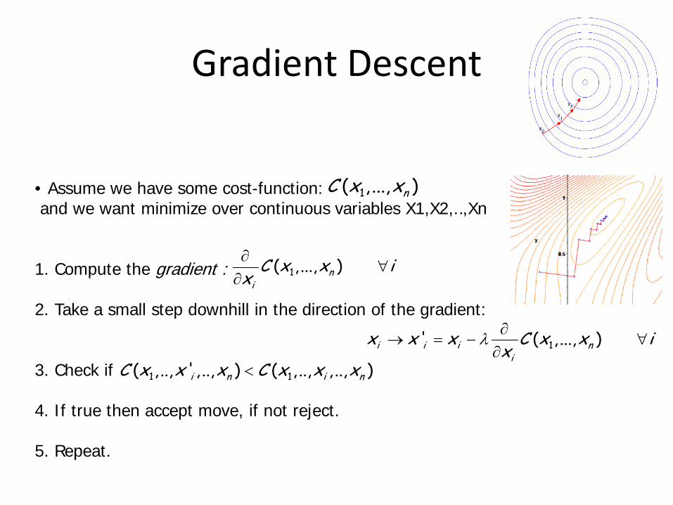
• Assume we have some cost-function: and we want minimize over continuous variables X1,X2,..,Xn

1. Compute the gradient : 2. Take a small step downhill in the direction of the gradient: 3. Check if 4. If true then accept move, if not reject. 5. Repeat.

1( , ..., )nC x x

1( ,..., )niC x x i

x∂

∀∂

1' ( ,..., )i i i ni

x x x C x x ix

λ ∂→ = − ∀

∂1 1( , .., ' ,.., ) ( ,.., , .., )i n i nC x x x C x x x<

Line Search

• In GD you need to choose a step-size. • Line search picks a direction, v, (say the gradient direction) and searches along that direction for the optimal step: • Repeated doubling can be used to effectively search for the optimal step:

• There are many methods to pick search direction v. Very good method is “conjugate gradients”.

η* = argmin C(xt +ηvt )

η →2η →4η →8η (until cost increases)

• Want to find the roots of f(x).

• To do that, we compute the tangent at Xn and compute where it crosses the x-axis.

• Optimization: find roots of

• Does not always converge & sometimes unstable.

• If it converges, it converges very fast

Basins of attraction for x5 − 1 = 0; darker means more iterations to converge.

)()()(0)( 1

1 n

nnn

nn

nn xf

xfxxxxxfxf

∇−=⇒

−−

=∇ ++

∇f (xn )

[ ])()()(0)( 1

1 n

nnn

nn

nn xf

xfxxxxxfxf

∇∇∇

−=⇒−

∇−=∇∇ +

+

Newton’s Method

Simulated annealing search

• Idea: escape local maxima by allowing some "bad" moves but gradually decrease their frequency.

• This is like smoothing the cost landscape.

Simulated annealing search

• Idea: escape local maxima by allowing some "bad" moves but gradually decrease their frequency

•

Properties of simulated annealing search

• One can prove: If T decreases slowly enough, then simulated annealing search will find a global optimum with probability approaching 1 (however, this may take VERY long)

– However, in any finite search space RANDOM GUESSING also will find a global optimum with probability approaching 1 .

• Widely used in VLSI layout, airline scheduling, etc.

Tabu Search

• A simple local search but with a memory.

• Recently visited states are added to a tabu-list and are temporarily excluded from being visited again. • This way, the solver moves away from already explored regions and (in principle) avoids getting stuck in local minima.

Local beam search • Keep track of k states rather than just one.

• Start with k randomly generated states.

• At each iteration, all the successors of all k states are generated.

• If any one is a goal state, stop; else select the k best successors from the

complete list and repeat. • Concentrates search effort in areas believed to be fruitful.

– May lose diversity as search progresses, resulting in wasted effort.

Genetic algorithms • A successor state is generated by combining two parent states

• Start with k randomly generated states (population)

• A state is represented as a string over a finite alphabet (often a string of 0s

and 1s)

• Evaluation function (fitness function). Higher values for better states.

• Produce the next generation of states by selection, crossover, and mutation

• Fitness function: number of non-attacking pairs of queens (min = 0, max = 8 × 7/2 = 28)

• P(child) = 24/(24+23+20+11) = 31% • P(child) = 23/(24+23+20+11) = 29% etc

fitness: #non-attacking queens

probability of being regenerated in next generation

Linear Programming

Problems of the sort:

maximize cT xsubject to : Ax ≤ b; Bx = c

• Very efficient “off-the-shelves” solvers are available for LRs. • They can solve large problems with thousands of variables.

Summary

• Local search maintains a complete solution – Seeks to find a consistent solution (also complete)

• Path search maintains a consistent solution – Seeks to find a complete solution (also consistent)

• Goal of both: complete and consistent solution – Strategy: maintain one condition, seek other

• Local search often works well on large problems – Abandons optimality – Always has some answer available (best found so far)

The importance of a good representation

• Properties of a good representation:

• Reveals important features • Hides irrelevant detail • Exposes useful constraints • Makes frequent operations easy-to-do • Supports local inferences from local features

• Called the “soda straw” principle or “locality” principle • Inference from features “through a soda straw”

• Rapidly or efficiently computable • It’s nice to be fast

Reveals important features / Hides irrelevant detail

• “You can’t learn what you can’t represent.” --- G. Sussman • In search: A man is traveling to market with a fox, a goose, and a

bag of oats. He comes to a river. The only way across the river is a boat that can hold the man and exactly one of the fox, goose or bag of oats. The fox will eat the goose if left alone with it, and the goose will eat the oats if left alone with it. How can the man get all his possessions safely across the river?

• A good representation makes this problem easy: 1110 0010 1010 1111 0001 0101

0000 1101

1011

0100 1110

0010 1010 1111

0001

0101

MFGO M = man F = fox G = goose O = oats 0 = starting side 1 = ending side

Exposes useful constraints

• “You can’t learn what you can’t represent.” --- G. Sussman • In logic: If the unicorn is mythical, then it is immortal, but if it

is not mythical, then it is a mortal mammal. If the unicorn is either immortal or a mammal, then it is horned. The unicorn is magical if it is horned. Prove that the unicorn is both magical and horned.

• A good representation makes this problem easy:

( ¬ Y ˅ ¬ R ) ^ ( Y ˅ R ) ^ ( Y ˅ M ) ^ ( R ˅ H ) ^ ( ¬ M ˅ H ) ^ ( ¬ H ˅ G )

1010 1111 0001 0101

Makes frequent operations easy-to-do

Roman numerals • M=1000, D=500, C=100, L=50, X=10, V=5, I=1 • 2000 = MM; 1776 = MDCCLXXVI

• Long division is very tedious (try MDCCLXXVI / XVI) • Testing for N < 1000 is very easy (first letter is not “M”)

Arabic numerals

• 0, 1, 2, 3, 4, 5, 6, 7, 8, 9, “.”

• Long division is much easier (try 1776 / 16) • Testing for N < 1000 is slightly harder (have to scan the string)

Supports local inferences from local features

• Linear vector of pixels = highly non-local inference for vision

• Rectangular array of pixels = local inference for vision

0 0 0 1 0 0 0 0 0 0 0 0 0 1 0 0 0 0 0 0 0 0 0 1 0 0 0 0 0 0 0 0 0 1 0 0 0 0 0 0 0 0 0 1 1 1 1 1 1 1 0 0 0 0 0 0 0 0 0 0 0 0 0 0 0 0 0 0 0 0 0 0 0 0 0 0 0 0 0 0

Corner!!

… … 0 1 0 … … 0 1 1 … … 0 0 0 … …

Corner??

Positive Examples | Negative Examples

*

*

*

Digital 3D Shape Representation

The Power of a Good Representation

Learning the “Multiple Instance” Problem

“Solving the multiple instance problem with axis-parallel rectangles”

Dietterich, Lathrop, Lozano-Perez, Artificial Intelligence 89(1997) 31-71

“Compass: A shape-based machine learning tool for drug design,” Jain, Dietterich, Lathrop, Chapman, Critchlow, Bauer, Webster, Lozano-Perez,

J. Of Computer-Aided Molecular Design, 8(1994) 635-652

From last class meeting – a “non-distance” heuristic

• The “N Colored Lights” search problem. – You have N lights that can change colors.

• Each light is one of M different colors.

– Initial state: Each light is a given color. – Actions: Change the color of a specific light.

• You don’t know what action changes which light. • You don’t know to what color the light changes. • Not all actions are available in all states.

– Transition Model: RESULT(s,a) = s’ where s’ differs from s by exactly one light’s color.

– Goal test: A desired color for each light.

• Find: Shortest action sequence to goal.

…

N=3 M=4

From last class meeting – a “non-distance” heuristic

• The “N Colored Lights” search problem. – Find: Shortest action sequence to goal.

• h(n) = number of lights the wrong color • f(n) = g(n) + h(n)

– f(n) = (under-) estimate of total path cost – g(n) = path cost so far = number of actions so far

• Is h(n) admissible? – Admissible = never overestimates the cost to the goal. – Yes, because: (a) each light that is the wrong color must change;

and (b) only one light changes at each action.

• Is h(n) consistent? – Consistent = h(n) ≤ c(n,a,n’) + h(n’), for n’ a successor of n. – Yes, because: (a) c(n,a,n’)=1; and (b) h(n) ≤ h(n’)+1

• Is A* search with heuristic h(n) optimal?

…

N=3 M=4